Computers & Fluids 110 (2015) 198–210

Contents lists available at ScienceDirect

Computers & Fluids

journal homepage: www.elsevier .com/locate /compfluid

Parallel hybrid PSO with CUDA for lD heat conduction equation

http://dx.doi.org/10.1016/j.compfluid.2014.05.0200045-7930/� 2014 Elsevier Ltd. All rights reserved.

⇑ Corresponding author.E-mail address: ztang@hnu.edu.cn (Z. Tang).

Aijia Ouyang a, Zhuo Tang a,⇑, Xu Zhou a, Yuming Xu a, Guo Pan a, Keqin Li a,b

a College of Information Science and Engineering, Hunan University, Changsha, Hunan 410082, Chinab Department of Computer Science, State University of New York at New Paltz, New Paltz, NY 12561, USA

a r t i c l e i n f o

Article history:Received 8 December 2013Received in revised form 6 May 2014Accepted 15 May 2014Available online 28 May 2014

Keywords:Heat conduction equationSpline difference methodParticle swarm optimizationConjugate gradient methodGPU

a b s t r a c t

Objectives: We propose a parallel hybrid particle swarm optimization (PHPSO) algorithm to reduce thecomputation cost because solving the one-dimensional (1D) heat conduction equation requires largecomputational cost which imposes a great challenge to both common hardware and softwareequipments.

Background: Over the past few years, GPUs have quickly emerged as inexpensive parallel processorsdue to their high computation power and low price, The CUDA library can be used by Fortran, C, C++,and by other languages and it is easily programmed. Using GPU and CUDA can efficiently reduce the com-putation time of solving heat conduction equation.

Methods: Firstly, a spline difference method is used to discrete 1D heat conduction equation into theform of linear equation systems, secondly, the system of linear equations is transformed into an uncon-strained optimization problem, finally, it is solved by using the PHPSO algorithm. The PHPSO is based onCUDA by hybridizing the PSO and conjugate gradient method (CGM).

Results: A numerical case is given to illustrate the effectiveness and efficiency of our proposed method.Comparison of three parallel algorithms shows that the PHPSO is competitive in terms of speedup andstandard deviation. The results also show that using PHPSO to solve the one-dimensional heat conductionequation can outperform two parallel algorithms as well as HPSO itself.

Conclusions: It is concluded that the PHPSO is an efficient and effective approach towards the 1D heatconduction equation, as it is shown to be with strong robustness and high speedup.

� 2014 Elsevier Ltd. All rights reserved.

1. Introduction

Recently, taking advantage of graphic processing capability,numerical simulation has become available via the utilization ofa GPU (graphics processing unit) instead of a CPU (central process-ing unit) [1]. In its initial stage, however, the GPU cannot be madeto communicate with an API (application programming interface)such as OpenGL and DirectX. In November 2006, NVIDIA unveiledthe industry’s first DirectX 10 GPU, the GeForce 8800 GTX. TheGeForce 8800 GTX was also the first GPU to be built with NVIDIAsCUDA (compute unified device architecture). Over the past fewyears, graphics processing units (GPUs) have quickly emerged asinexpensive parallel processors due to their high computationpower and low price [2,3]. The CUDA library can be used by For-tran, C, C++, and by other languages and it is easily programmed.Graphics processing units (GPU) technique has been applied tolarge-scale social networks [4], smoothed particle hydrodynamics

simulations [5], volume visualization [6], hopfield neural network[7], particle filters [8], robotic map [9], finite difference schemes[10,11], object recognition [12], thermal analysis [13], hydrody-namic simulations [14], thermodynamic systems [15], solidifica-tion process simulation [16], computational fluid dynamics[17,18], particle simulation [19,20].

The one-dimensional heat conduction equation is a well-known simple second order linear partial differential equation(PDE) [21–24]. PDEs like the heat conduction equation often arisein modeling problems in science and engineering. It is also usedin financial mathematics in the modeling of options. Forexample, the Black–Scholes option pricing model’s differentialequation can be transformed into the heat conduction equation[25,26].

Over the last few years, many physical phenomena were formu-lated into nonlocal mathematical model. These physical phenom-ena are modeled by nonclassical parabolic initial-boundary valueproblems in one space variable which involve an integral term overthe spatial domain of a function of desired solution. This integralterm may appear in a boundary condition, which is called nonlocal,or in the governing partial differential equation itself, which is

A. Ouyang et al. / Computers & Fluids 110 (2015) 198–210 199

often referred to as a partial integro-differential equation, or inboth [27].

The presence of an integral term in a boundary condition cangreatly complicate the application of standard numerical tech-niques such as finite difference procedures, finite element methods,spectral techniques, and boundary integral equation schemes.Therefore, it is essential that nonlocal boundary value problemscan be converted a more desirable form and to make them moreapplicable to problems of practical interest.

Recently, nonlocal boundary value problems have been coveredin the literature [28–31]. For instance, Dehghan [32] presented anew finite difference technique for solving the one-dimensionalheat conduction equation subject to the specification of mass,but their methods are only first-order accurate. Caglar et al. [33]developed a third degree B-spines method to solve the heatconduction Eqs. (1)–(3) with the accuracy of Oðk2 þ h2Þ, and atthe endpoints, the approximation order is second order only. Liuet al. [34] used a quartic spline method to solve one-dimensionaltelegraphic equations, we consider the lD heat conduction equa-tion in accordance with the above method. Tsourkas and Rubinskyused a parallel genetic algorithm for solving heat conduction prob-lems [35,36].

It is well-known that genetic algorithm is a classic evolution-ary algorithm.It has been successfully applied to all kinds of realproblems, such asoptimizing system state in a cloud system[37]. PSO is also an evolutionary algorithm and it is developedby Dr.Eberhart and Dr. Kennedy in 1995, inspired by social behav-ior ofbird flocking or fish schooling. PSO has an outstandingperfor-mance in optimizing functions. Integrating the successful methodsand efficient hybrid strategies, we present a PHPSO algorithmbased on CUDA for the one-dimensional heat conduction equa-tion. This paper has some contributions, which are described asfollows.

1. A new method for solving the one-dimensional heat conductionequation with the nonlocal boundary value conditions is con-structed by using quartic spline functions. It shows that theaccuracy of the presented method can reach Oðk2 þ h4Þ at theinterior nodal points.

2. We also obtain a new method to deal with the nonlocal bound-ary conditions with the accuracy being Oðkþ h4Þ. It is much bet-ter than the classical finite difference method with the accuracyof Oðkþ h2Þ.

3. We design a parallel hybrid algorithm by hybridizing the PSOand CGM with the CUDA technique. Such an algorithm canspeed up the convergence to the optimum solution.

The remainder of this paper is organized in the following way.Section 2 gives a detailed theoretical analysis and mathematicalproof concerning the 1D heat conduction equation. Section 3shows the process of transforming a system linear systems intoan unconstrained optimization problem. In Section 4, the serialalgorithms of PSO and CGM are presented. In Section 5, the archi-tecture of CUDA is introduced first, and a parallel PSO algorithm, aparallel CGM algorithm, and a parallel hybrid PSO algorithm areproposed respectively in detail. Section 6 displays the experimen-tal results and discussions. Finally, the paper concludes withSection 7.

2. Method of numerical processing

2.1. Mathematical model

We consider the one-dimensional nonclassical heat conductionequation

@u@t¼ a

@2u@x2 ; 0 < x < 1; 0 < t 6 T; ð1Þ

with initial conditions

uðx;0Þ ¼ f ðxÞ; 0 6 x 6 1; ð2Þ@u@x

uð1; tÞ ¼ gðtÞ; 0 < t 6 T; ð3Þ

and a nonlocal conditionR b0 uðx; tÞdx ¼ mðtÞ;

0 < t 6 T; 0 < b < 1:ð4Þ

In this problem, f ðxÞ; gðtÞ and mðtÞ are given functions and aand b are constants. If b ¼ 1, Eq. (4) can be differentiated as

m0ðtÞ ¼Z 1

0utdx ¼

Z 1

0auxxdx ¼ auxð1; tÞ � auxð0; tÞ: ð5Þ

The derivation holds only when m and u are differentiable.

2.2. Quartic spline and interpolation error

Let P be a uniform partition of ½0;1� as follows

0 ¼ x0 < x1 < � � � < xn ¼ 1; ð6Þ

where xi ¼ ih; h ¼ 1=n.The quartic spline space on ½0;1� is defined as

S34ðPÞ ¼ s 2 C3½0;1� : sj½xi�1 ;xi � 2 P4; i ¼ 1ð1Þn

n o;

where Pd is the set of polynomials of degree at most d.It is easy to know that dim S3

4ðPÞ ¼ nþ 4. For any s 2 S34ðPÞ, the

restriction of s in ½xi�1; xi� can be expressed as

sðxÞ ¼ si�1 þ hs0i�1t þ h2s00i�1t2

12ð6� t2Þ þ h2s00i

t4

12þ h3s000i�1

t3

12ð2� tÞ;

ð7Þ

where x ¼ xi�1 þ th, t 2 ½0;1�, si ¼ sðxiÞ; s0i ¼ s0ðxiÞ, s00i ¼ s00ðxiÞ;s000i ¼ s000ðxiÞ; i ¼ 0ð1Þn.

This leads to

si ¼ si�1 þ hs0i�1 þ5

12h2s00i�1 þ

112

h2s00i þ1

12h3s000i�1; ð8Þ

s0i ¼ s0i�1 þ23

hs00i�1 þ13

hs00i þ16

h2s000i�1; ð9Þ

s000i ¼ �s000i�1 þ2h

s00i � s00i�1

� �; ð10Þ

for i ¼ 1ð1Þn. Based on the above three equations, we can have

112

s00iþ1 þ56

s00i þ1

12s00i�1 ¼

1

h2 ½siþ1 � 2si þ si�1�; i ¼ 1ð1Þn� 1: ð11Þ

Likewise, if we write the quartic spline function s in ½xi�1; xi� asfollows

sðxÞ ¼ si þ hs0it þ h2s00it2

12ð6� t2Þ þ h2s00i�1

t4

12þ h3s000i

t3

12ð2þ tÞ;

ð12Þ

where x ¼ xi þ th; t 2 ½�1;0�. This leads to

si�1 ¼ si � hs0i þ5

12h2s00i þ

112

h2s00i�1 þ1

12h3s000i ; ð13Þ

s0i�1 ¼ s0i �23

hs00i �13

hs00i�1 þ16

h2s000i ; ð14Þ

s000i�1 ¼ �s000i þ2h

s00i � s00i�1

� �; ð15Þ

for i ¼ 1ð1Þn.

200 A. Ouyang et al. / Computers & Fluids 110 (2015) 198–210

Denote DisðxÞ ¼ sðiÞðxÞ. We have

si�1 ¼ si � hs0i þ12

h2s00i � � � � ¼ e�hDsi: ð16Þ

Then Eq. (11) can be rewritten as

112½ehD þ 10þ e�hD�s00i ¼

1

h2 ½ehD � 2þ e�hD�si; i ¼ 1ð1Þn� 1: ð17Þ

Equivalently,

s00i ¼12

h2

ehD � 2þ e�hD

ehD þ 10þ e�hDsi; i ¼ 1ð1Þn� 1: ð18Þ

Theorem 1. Assume that gðxÞ is sufficiently smooth in the interval½0;1�. Let s 2 S3

4ðPÞ be the quartic spline which interpolates gðxÞ asfollows

si ¼ gðxiÞ; i ¼ 0ð1Þn; ð19Þ

s00n ¼ g00ðxnÞ;

s00 þh2

12s0000 ¼ g0ðx0Þ þ

h2

12g000ðx0Þ;

s0n �h2

12s000n ¼ g0ðxnÞ �

h2

12g000ðxnÞ:

ð20Þ

Then we have

s00i ¼ g00ðxiÞ �1

240h4gð6ÞðxiÞ þ Oðh6Þ; i ¼ 1ð1Þn� 1; ð21Þ

g00 ¼g1 � g0

h� 1

12hg001 �

512

hg000 �1

12h2g0000 þ Oðh4Þ; ð22Þ

g0n ¼gn � gn�1

hþ 5

12hg00n þ

112

hg00n�1 þ1

12h2g000n þ Oðh4Þ; ð23Þ

where gi ¼ gðxiÞ; g0i ¼ g0ðxiÞ, g00i ¼ g00ðxiÞ; g000i ¼ g000ðxiÞ; i ¼ 0ð1Þn.

Proof. The proof of Eq. (21) can been seen in [38].

From Eqs. (11) and (19), we can get

ðe2Dh þ 10eDh þ 1Þs000 ¼12

h2 ðe2Dh � 2eDh þ 1Þg000: ð24Þ

Then, similar to the proof of Eq. (21), we can obtain the followingresult

s000 ¼ g00ðx0Þ þ Oðh4Þ: ð25Þ

Then, according to Eqs. (8) and (20), we have

g00 þh2

12g0000 ¼ s00 þ

h2

12s0000 ¼

s1 � s0

h� 1

12hs001 �

512

hs000

¼ g1 � g0

h� 1

12hg001 �

512

hg000 þ Oðh4Þ: ð26Þ

Thus, Eq. (22) holds. Similarly, by using Eq. (13), we can prove Eq.(23). h

2.3. Quartic spline method

We consider the following heat conduction Eq. (1) with the ini-tial boundary value conditions (2) and (3) and derivative boundarycondition (5).

The domain ½0;1� � ½0; T� is divided into an n�m mesh with thespatial step size h ¼ 1=n in x direction and the time step sizek ¼ T=m, respectively.

Grid points ðxi; tjÞ are defined by

xi ¼ ih; i ¼ 0ð1Þn; ð27Þtj ¼ jk; j ¼ 0ð1Þm; ð28Þ

in which n and m are integers.Let sðxi; tjÞ and Uj

i be approximations to uðxi; tjÞ and

MiðtÞ ¼ @2sðx;tÞ@x2

���ðxi ;tÞ

, respectively.

Assume that uðx; tÞ is the exact solution to Eq. (1). For any fixedt, let sðx; tÞ 2 S3

4ðPÞ be the quartic spline interpolating to uðx; tÞ as in

sðxi; tÞ ¼ uðxi; tÞ; i ¼ 0ð1Þn; ð29Þ

@2s@x2

�����ðxn; tÞ ¼@2u@x2

�����ðxn; tÞ; ð30Þ

@s@x

����ðx0; tÞ þ1

12h2 @

3s@x3

�����ðx0; tÞ ¼@u@x

����ðx0; tÞ þ1

12h2 @

3u@x3

�����ðx0; tÞ; ð31Þ

@s@x

����ðxn; tÞ �1

12h2@

3s@x3

�����ðxn; tÞ ¼@u@x

����ðxn; tÞ �1

12h2 @

3u@x3

�����ðxn; tÞ: ð32Þ

Then it follows from Theorem 1 that

@2u@x2 jðxi; tÞ ¼

@2s@x2

�����ðxi; tÞ þ Oðh4Þ; i ¼ 1ð1Þn� 1: ð33Þ

For any fixed t, by using the Taylor series expansion, Eq. (1) canbe discretized at the point ðxi; tjÞ into

uðxi;tjþ1Þ�uðxi;tjÞk

¼12a

@2sðx;tÞ@x2

!j

i

þ @2sðx;tÞ@x2

!jþ1

i

24

35þOðk2þh4Þ;

ð34Þ

where i ¼ 1ð1Þn� 1; j ¼ 0ð1Þm� 1.Substituting (34) into spline relation (11) and using Eq. (29), we

conclude

ð1� 6arÞuðxiþ1; tjþ1Þ þ ð10þ 12arÞuðxi; tjþ1Þþ ð1� 6arÞuðxi�1; tjþ1Þ¼ 1þ 6arÞuðxiþ1; tjÞ þ ð10� 12arÞuðxi; tjÞþ ð1þ 6arÞuðxi�1; tjÞ þ Oðk2 þ h4Þ; ð35Þ

where r ¼ a kh2.

Neglecting the error term, we can get the following differencescheme

ð1� 6arÞUjþ1iþ1 þ ð10þ 12arÞUjþ1

i þ ð1� 6arÞUjþ1i�1

¼ ð1þ 6arÞUjiþ1 þ ð10� 12arÞUj

i þ ð1þ 6arÞUji�1;

i ¼ 1ð1Þn� 1; j ¼ 0ð1Þm; ð36Þ

with the accuracy being Oðk2 þ h4Þ.It is evident that the difference scheme (36) identifies the clas-

sical fourth order compact difference scheme, which is uncondi-tionally stable.

2.4. The difference scheme on the boundary

From the interpolation conditions (30)–(32) and Theorem 1, foreach t > 0, we have

@uðx0; tÞ@x

¼ uðx1; tÞ � uðx0; tÞh

� 112

h@2uðx1; tÞ

@x2 � 512

h@2uðx0; tÞ

@x2

� 112

h2 @3uðx0; tÞ@x3 þ Oðh4Þ; ð37Þ

A. Ouyang et al. / Computers & Fluids 110 (2015) 198–210 201

@uðxn; tÞ@x

¼ uðxn; tÞ � uðxn�1; tÞh

þ 512

h@2uðxn; tÞ

@x2 þ 112

h

� @2uðxn�1; tÞ@x2 þ 1

12h2 @

3uðxn; tÞ@x3 þ Oðh4Þ: ð38Þ

Let t ¼ tjþ1, it follows form Eqs. (1) and (37) that

uxðx0; tjþ1Þ ¼uðx1; tjþ1Þ � uðx0; tjþ1Þ

h� 1

12ah

� uðx1; tjþ1Þ � uðx1; tjÞk

� 512a

h

� uðx0; tjþ1Þ � uðx0; tjÞk

� 112

h2 @3uðx0; tjþ1Þ@x3

þ Oðkþ h4Þ: ð39Þ

From Eqs. (1), (3) and (5), we can get

@3uð0; tÞ@x3 ¼ 1

a@2uð0; tÞ@x@t

¼ 1a2 m00ðtÞ � 1

ag0ðtÞ: ð40Þ

Substituting (40) into (39) and neglecting the error term, we get thefourth-order difference scheme at x ¼ x0

1� 112r

� �Ujþ1

1 � 1þ 512r

� �Ujþ1

0 þ 112r

Uj1 þ

512r

Uj0

¼ huxð0; tjþ1Þ þ1

12h3 1

a2 m00ðtjþ1Þ �1a

g0ðtjþ1Þ� �

: ð41Þ

Similarly, the difference scheme at the other end x ¼ xn is

1þ 512r

� �Ujþ1

n þ �1þ 112r

� �Ujþ1

n�1 �5

12rUj

n þ1

12rUj

n�1

¼ huxð1; tjþ1Þ �1

12ah3g0ðtjþ1Þ: ð42Þ

3. Derivation of objective function

The formula of a system linear systems is shown as follows:

AX ¼ B; ð43Þ

or

XN

j¼1

aijxj ¼ bi; i ¼ 1;2; . . . ;M: ð44Þ

In the above formula, A ¼ ðaijÞM�N 2 RM�N is a matrix,X ¼ ðx1; x2; . . . ; xNÞT is a vector, B ¼ ðb1; b2; . . . ; bMÞT is also avector.

Set the absolute error of X and B be respectively dX and dB. Sothe relative error of X can be estimated as follow:

kdXk=kXk 6 KðAÞkdBk=kBk: ð45Þ

If we obtain the L2 norm for the above formula, the condition num-ber of matrix A is:

KðAÞ ¼ rmax=rmin: ð46Þ

In the formula, rmax and rmin is respectively the maximumand minimum of singular value of matrix A. If KðAÞ is very large,the formula (43) is morbid state linear equation group. The char-acteristic of morbid state linear equation group is: even though Aand B are little changed, the solution of them will be greatlydifferent.

To use PSO to solve linear equation group (43), we transformthe linear equation group problem into an unconstrained optimiza-

tion problem. Obviously, the L1 norm of linear equation group (43)is the optimal solution of the problem (47). Both of them arecompletely equivalent. The formula of the problem is shown asfollows:

min E ¼ minXm

i¼1

XN

j¼1

jaijxj � bij: ð47Þ

Consequently, we set the fitness function as follows:

f ðxÞ ¼ minXm

i¼1

XN

j¼1

jaijxj � bij; ð48Þ

in formula (48), The solution vector X ¼ ðxi; x2; . . . ; xnÞ is composedby xjðj ¼ 1;2; . . . ;NÞ. X is a real vector.

4. Serial algorithms

4.1. Particle swarm optimization

Particle swarm optimization (PSO), a swarm intelligence algo-rithm to solve optimization problems, is initialized randomly witha cluster of particles, after which it searches for optimal value bymeans of updating generations [39]. Given that the search spaceis D-dimensional, the population is composed of many particles.Particle i refers to the i-th particle in the population, which isdenoted by D-dimensional vector Xi ¼ ðxi1; xi2; . . . ; xiDÞT . V denotes

the search velocity of particles, and Vi ¼ ðv i1;v i2; . . . ;v iDÞT revealsthe search velocity of particle i. The visited positions of particles

are denoted by P, and Pi ¼ ðpi1; pi2; . . . ; piDÞT reveals local best posi-

tion, and it is the best previously visited position of particle i. Theglobal best position is represented by G ¼ ðg1; g2; . . . ; gDÞ

T , whichshows the optimal of all local best positions among the population.At each step, the search velocity of all particles and their local bestposition will be given a value according to Eqs. (49) and (50), theprocess goes repeatedly till a user-defined stopping criterion ismet.

vkþ1id ¼ xvk

id þ c1r1 ptid � xk

id

� �þ c2r2 gk

id � xkid

� �; ð49Þ

xkþ1id ¼ xk

id þ vkþ1id : ð50Þ

Here, k indicates the current iterative step, i 2 f1;2; . . . ;Ng,and d 2 f1;2; . . . ;Dg;N refers to the number of the total popula-tions. r1 and r2 represent independently uniformly distributedrandom variables with a range of ð0;1Þ; c1 and c2 denote theacceleration constants, and x refers to the inertia weight factor[40].

4.2. Conjugate gradient method

The CGM is one of the most popular iterative methodsdedicated to solving linear systems of equations with sparse,symmetric and positive-definite matrix of coefficients. A versionof the CGM algorithm implemented in this study is shown inAlgorithm 1.

The main steps of CGM for an unconstrained optimizationproblem are as follows:

Step 1. Set a initial point xð0Þ, and precision definition e > 0.Step 2. If krf ðxð0ÞÞk 6 e, stop computation, the minimum point is

xð0Þ, otherwise, go to Step 3.Step 3. Let pð0Þ ¼ �rf ðxð0ÞÞ, and set k ¼ 0.Step 4. Use one dimensional search to solve tk, obtain

f ðxðkÞ þ tkpðkÞÞ ¼min f ðxðkÞ þ tpðkÞÞ; t P 0, let xðkþ1Þ ¼ xðkÞ

þtkpðkÞ, go to Step 5.

202 A. Ouyang et al. / Computers & Fluids 110 (2015) 198–210

Step 5. If krf ðxðkþ1ÞÞk 6 e, stop computation, the minimum pointis xðkþ1Þ, otherwise, go to Step 6.

Step 6. If kþ 1 ¼ n, let xð0Þ ¼ xðnÞ, go to Step 3, otherwise, go toStep 7.

Step 7. Let pðkþ1Þ ¼ �rf ðxðkþ1ÞÞ þ kkpðkÞ, kk ¼ krf ðxðkþ1ÞÞkkrf ðxðkÞÞk , let k ¼ kþ 1,

go to Step 4.

Algorithm 1. Conjugate gradient method

Input: A; b;nOutput: xkþ1

1: r0 :¼ b� Ax0

2: p0 :¼ r0

3: k :¼ 14: while k <¼ n do

5: ak :¼ rTk rk

PTk APk

6: xKþ1 : xk þ akPk

7: rKþ1 : rk � akAPk

8: if rkþ1 < m then

9: bk :¼ rTkþ1rkþ1

rTk

rk

10: pkþ1 :¼ rkþ1 þ bkPk

11: k :¼ kþ 112: end if13: end while14: Output solution

GPU kernel 1

CPU serial code

GPU kernel 2

Host Device

Block(0, 0)

Block(0, 1)

Block(0, 2)

Block(1, 0)

Block(1, 1)

Block(1, 2)

Grid 1

Reg

iste

rL

ocal

mem

ory

Shar

ed m

emor

yC

onst

ant m

emor

yT

extu

re m

emor

y

Glo

bal m

emor

y

Grid 2

Thread(0, 1)

Thread(0, 2)

Thread(1, 0)

Thread(1, 1)

Thread(1, 2)

Thread(2, 0)

Thread(2, 1)

Thread(2, 2)

Thread(0, 0)

Block(1, 1)

Fig. 1. The architecture of CUDA.

4.3. Hybrid particle swarm optimization

The global search ability of the basic PSO is extremely strongwhile the local search ability is extremely weak, which is exactlythe opposite of the CGM. To overcome the shortcomings of thetwo algorithms and utilize only their advantages, we present ahybrid particle swarm optimization (HPSO) algorithm, in whichthe CGM is incorporated into the basic PSO. In the HPSO, becausethe CGM is a local algorithm, it can obtain the optimal value withno need to calculate the derivative of fitness function; therefore,based on the original PSO, only a decent computation cost is added.In addition, each particle in the population is regarded as a point ofthe CGM and each iteration of HPSO has two parts: the CGM partand PSO part. In each iteration, all particles are updated, and theelite individual generated by PSO algorithm will be replaced bythe best individual generated by CGM. In this way, the accuracyof searching the position in each HPSO iteration is improved.Therefore, the HPSO not only has higher precision but also helpsto obtain a faster convergent speed compared with the originalPSO and CGM.

The main steps of HPSO for an unconstrained optimizationproblem are as follows:

Step 1. Initialize the parameters of population, such as, populationsize, position, velocity, acceleration factor, and inertiaweight factor.

Step 2. Compute the fitness value of each particle.Step 3. Find the local optimum and the global optimum.Step 4. Update the velocity and position of each particle.Step 5. Compute the fitness value of population.Step 6. Update the local optimum and the global optimum.Step 7. Execute a local search precisely by CGM for the individual

of global optimum in the population of HPSO.Step 8. If the termination criteria are satisfied, output results and

terminate the HPSO algorithm; otherwise, go to Step 4.

Algorithm 2. Particle swarm optimization

Input: xmin; xmax;G;D;N; p; lbp; gbp; f ; lbf ; gbf ;vOutput: gbp0; gbf 0

1: Initialize parameters p; lbp, and v2: Compute fitness f3: Find lbp and gbp4: for g ¼ 1 : G do5: Update v and p6: Evaluate fitness f7: Update lbp and gbp8: end for9: Output gbp and gbf

Algorithm 3. Hybrid particle swarm optimization

Input: xmin; xmax;G;D;N; p; lbp; gbp; f ; lbf ; gbf ;vOutput: gbp0; gbf 0

1: Initialize parameters p; lbp, and v2: Compute fitness f3: Find lbp and gbp4: for g ¼ 1 : G do5: Update v and p6: Evaluate fitness f7: Update lbp and gbp8: Execute local search of CGM9: end for

10: Output gbp and gbf

5. Parallel algorithms

5.1. The architecture of CUDA

We describe in brief the CUDA architecture in this subsection; bythis means, we hope that to comprehend the design of our presentedGPU implementation can become easier. A GPU is a multi-core,multi-threaded highly parallel processor with enormouscomputing power. The NVIDIA Corporation released the CUDAframework to help users develop software for their GPUs. Thearchitecture of CUDA is designed around a scalable array of multi-processors as shown in Fig. 1, which is based on a SIMT programming

Table 1Specifications of GPU.

Parameter GTX 465 C2050

Number of stream processors 352 448Global memory size (GB) 1 2.62Shared memory size (KB) 48 48Constant memory size (KB) 64 64Memory bus width (bits) 256 384Memory bandwidth (GB/s) 102.6 144Memory clock rate (MHz) 802 1536Estimated peak performance (Gflops) 855.4 1030GPU clock rate (MHz) 0.6 1.15Warp Size 32 32Maximum number of threads per MP 1024 1024CUDA compute capability 2.0 2.0

Fig. 2. Flowchart of PPSO.

A. Ouyang et al. / Computers & Fluids 110 (2015) 198–210 203

modal. A parallel program on a GPU (also termed device) is inter-leaved with a serial one executed on the CPU (also termed host). Athread block has a stream of threads executed concurrently on amultiprocessor, which has synchronized access to a shared memory.However, threads originating from different blocks cannot be coop-erated in this way. These threads are combined to form a grid.Threads in a grid are enumerated and distributed to multiprocessorwhen a CUDA code on the CPU calls a kernel function. All the threadsin the grid can access the same global memory. Two additional read-only memory spaces are accessible by all the threads, the constantmemory and texture one (see Table 1).

5.2. Parallel particle swarm optimization

In this section, we would like to explain the meaning of eachkernel function in detail with its pseudo code attached. There arefive kernel functions in the PPSO algorithm, and they are imple-mented in GPU. The flow chart of PPSO is shown in Fig. 2.

5.2.1. Kernel function dev_rndThe purpose of dev rnd is to generate a random number

sequence of initial state. Each thread is a complex variable, whichneeds to contain curand library files and curand kernel, and call thelibrary function curand init to generate high quality pseudo-random number. Given the differenced between seeds,curand init would produce different initial states and sequence.Each thread is assigned a unique serial number.

Sequences generated with different seeds usually do not havestatistically correlated values, but some choices of seeds may resultin statistically correlated sequences. Sequences generated with thesame seed and different sequence numbers will not have statisti-cally correlated values. For the highest quality parallel pseudo-ran-dom number generation, each experiment should be assigned aunique seed. Within an experiment, each thread of computationshould be assigned a unique sequence number. If an experimentspans multiple kernel launches, it is recommended that threadsbetween kernel launches be given the same seed, and sequencenumbers be assigned in a monotonically increasing way. If the sameconfiguration of threads is launched, random state can be preservedin global memory between launches to avoid state setup time [41].

Experiments have shown that the random function incurand library has better quality and higher efficiency than thatgenerated by the rand function of CPU.

5.2.2. Kernel function initInit is used to initialize a particle position, velocity, and the indi-

vidual best position in populations according to the formula in thePSO. Every thread in thread blocks represents a complex variable.Each row in the grid represents a particle. After defining xid

dimension index, index of population yid, thread (namely, eachposition variable) position in the whole grid posID, we call

curand uniformðÞ to generate two random numbers stochasticallyand uniformly distributed between 0.0 and 1.0, and then use themto initialize the position and velocity respectively.

5.2.3. Kernel function UpdateUpdate is used to modify the position, individual optimal posi-

tion and velocity of each particle in the population for each thread.As for the parameter setting, it is the same as init. It firstly updatesthe individual optimal position according to the modifying mark,and then respectively calls curand uniform to generate two randomnumbers between two 0.0 and 1.0 respectively. They are used togenerate a new particle velocity, further update particle position,and reinitialize the numbers exceeding the limits at the same time.

5.2.4. Kernel function FindgbfFindgbf is used to update the individual optimal position, and

find the global optimal index and global optimal fitness. A particleis a thread. In this paper, the population numbers are set less than512, thus a thread block is a whole population. We give full play tothe advantages of shared memorizer and registers. First, we need todefine the thread pid and shared memorizer variable s and registervariable t, and then initialize s and t in accordance with differentrequirements. If the initial mark flag ¼ 0, the fitness value f shouldbe copied directly to individual extremum lbf, otherwise, lbf andmodifying mark g u should be modified correspondingly after com-parison. Then we need to call device function reduceToMaxðs; pidÞ orreduceToMinðs; pidÞ to operate and summarize according to themaximum or minimum value for parallel reduction, in order to findthe group extremum gbf, and ultimately the global optimal indexID. The skill is that we should set t to the maximum number ofthreads that are not the group extremum gbf, otherwise t wouldbe the thread number of gbf. Then we should reuse shared memo-rizer and call reduceToMinðs; pidÞ to execute the reduction thenassign the first thread to ID. If the most optimal value of thisgeneration is not superior to group optimal value gbf, ID would beP, which means there is no need to update the best position gp of

204 A. Ouyang et al. / Computers & Fluids 110 (2015) 198–210

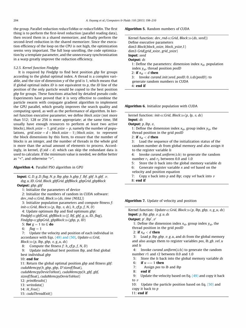
the group. Parallel reduction reduceToMax or reduceToMin. The firstthing is to perform the first-level reduction (parallel reading data),then record them in a shared memorizer, and finally perform thesecond-level reduction in the shared memorizer. Since the execu-tion efficiency of the loop on the CPU is not high, the optimizationseems very important. The full loop unrolling, the code optimiza-tion by a template parameter, and the unnecessary synchronizationin a warp greatly improve the reduction efficiency.

5.2.5. Kernel function FindgbpIt is required by Findgbp to find best position gbp for groups

according to the global optimal index. A thread is a complex vari-able, and the size of dimension y of the grid is 1, which means thatif global optimal index ID is not equivalent to p, the ID line of theposition of the only particle would be copied to the best positiongbp for groups. These functions attached by detailed pseudo code.Experiments have proved that it is very effective to combine theparticle swarm with conjugate gradient algorithm to implementthe GPU parallel, which greatly improves the search quality andcomputing speed, as well as the performance of algorithm. In ker-nel function executive parameter, we define block xsize (not morethan 512; 128 or 256 is more appropriate; at the same time, SMusually have enough resources to perform at least two activeblocks), block ysize ¼ 1; grid ysize ¼ p, namely the number of popu-lations, grid xsize ¼ dþ block xsize� 1Þ=block xsize, to representthe block dimensions by this form, to ensure that the number ofblocks is an integer, and the number of threads in the whole gridis more than the actual amount of elements to process. Accord-ingly, in kernel, if ðxid < dÞ which can skip the redundant data isused to calculate. If the minimum value is needed, we define betteras ‘‘<’’, and otherwise ‘‘>’’.

Algorithm 4. Parallel PSO algorithm in GPU

Input: G;D; g D; flag;N; p; lbp; gbp;h gbp; f ; lbf ; gbf ;h gbf ;v;dsg u; ID;Grid;Block; gbfGrid; gbfBlock; gbpGrid; gbpBlock

Output: gbp; gbf1: Initialize the parameters of device2: Initialize the numbers of random in CUDA software:

dev_rndnGrid, Blocko(ds, time (NULL))3: Initialize population parameters and compute fitness f:

initnGrid, Blocko(p, lbp, v, ds), h_cf(p, f, N, D)4: Update optimum lbp and find optimum gbp:

FindgbfngbfGrid, gbfBlocko(f, lbf, gbf, g_u, ID, flag),FindgbpngbpGrid, gbpBlocko(gbp, p, ID)5: for g ¼ 1 to G do6: flag ¼ 17: Update the velocity and position of each individual in

accordance with Eqs. (49) and (50), UpdatenGrid,Blocko(p, lbp, gbp, v, g_u, ds)8: Compute the fitness f: h_cf(p, f, N, D)9: Update individual best position lbp, and find global

best individual gbp10: end for11: Return the global optimal position gbp and fitness gbf:cudaMemcpy(h_gbp, gbp, D⁄sizeof(float),cudaMemcpyDevieToHost), cudaMemcpy(h_gbf, gbf,sizeof(float), cudaMemcpyDevieToHost)12: printResults()13: writedata()14: H_Free()15: cudaThreadExit()

Algorithm 5. Random numbers of CUDA

Kernel function: dev_rndnGrid, Blocko(ds, seed))Define executive parametersdim3 Block(block_xsize, block_ysize,1)dim3 Grid(grid_xsize, grid_ysize)Input: seedOutput: ds

1: Define the parameters: dimension index xid, populationindex yid, thread position posID2: if xid < d then3: Invoke curand initðseed; posID;0;&ds½posID�Þ togenerate random numbers in CUDA4: end if

Algorithm 6. Initialize population with CUDA

kernel function: initnGrid, Blocko(p, lp, v, ds)Input: dsOutput: p; lbp;v ,

1: Define the dimension index xid, group index yid, thethread position in the grid posID2: if xid < d then3: Load the sequence of the initialization status of therandom number ds from global memory and also assign itto the register variable ls4: Invoke curand uniformð&lsÞ to generate the randomnumber r1 and r2 between 0.0 and 1.05: Store the ls back into the global memory variable ds6: Generate register variable x and vel based on thevelocity and position equation7: Copy x back into p and lbp; copy vel back into v8: end if

Algorithm 7. Update of velocity and position

Kernel function: UpdatenGrid, Blocko(p, lbp, gbp, v, g_u, ds)Input: p; lbp; gbp;v; g u; dsOutput: p0; lbp0;v 0

1: Define the dimension index xid, group index yid, thethread position in the grid posID2: if xid < d then3: Load p; lbp; gbp;v ; g u, and ds from the global memory

and also assign them to register variables pos, lb; gb;vel;uand ls4: Invoke curand uniform(&ls) to generate the random

number r1 and r2 between 0.0 and 1.05: Store the ls back into the global memory variable ds6: if u ¼¼ 1 then7: Assign pos to lb and lbp8: end if9: Update the velocity based on Eq. (49) and copy it back

to v10: Update the particle position based on Eq. (50) andcopy it back to p11: end if

Fig. 3. Flowchart of PCGM.

A. Ouyang et al. / Computers & Fluids 110 (2015) 198–210 205

Algorithm 8. Update of local and global optimum

Kernel function: FindgbfngbfGrid, gbfBlocko(f, lbf, gbf, g_u,ID, flag)Define executive parametersdim3 gbfGridð1;1Þdim3 gbfBlockðdev_P;1;1ÞInput: f ; lbf ; gbp;v ; g u; ds; flagOutput: f 0; lbf 0; gbf ; g u0; ID

1: Define the thread or particle index tid

2: Initialize the shared memory vector s and registervariable bf. To get the maximum value, it will be valued as0. To get the minimum value, it will be valued as 1E�203: if tid < N then4: Load f from global memory and assign it to s and bf5: Synchronization6: if flag ¼¼ 0 then7: Copy the bf to the individual best fitness lbf8: else9: Load lbf from global memory and assign it to the

register variable bf 110: Assign the ‘‘bf better bf 1’’ to register variableupdate and copy it back to g u11: if update ¼¼ 1 then12: Replace the individual optimum using newfitness13: end if14: end if15: if MAXIMIZE then16: reduceToMax < dev N > ðs; tidÞ17: else18: reduceToMin < dev N > ðs; t idÞ19: end if20: if flag ¼¼ 0jjðflag ¼¼ 1&&s½0�better � gbf Þ then21: if t id ¼¼ 0 then22: Assign the best fitness to the global best value23: end if24: Assign thread index of the best value to the bf, orthe bf valued as dev N; Assign the bf to the shared memoryvariable s25: reduceToMin < dev N > ðs; t idÞ26: Copy the best value index s½0� back into the ID27: else28: ID ¼ N29: end if30: end if

Algorithm 9. Search global optimal position

Kernel function: FindgbpngbpGrid, gbpBlocko(gbp, p, ID)Define executive parametersdim3 gbpBlockðblock xsize;1;1Þdim3 gbpGridðgrid xsize;1ÞInput: p; ID; dOutput: gbp

1: Define the dimension index xid

2: if xid < D && ID! ¼ N then3: Assign the solution of the No. ID particle in the p to theglobal best position gbp4: end if

5.3. Parallel conjugate gradient method

Conjugate gradient is a method which lies between thesteepest descent method and Newton method. It only needsfirst derivative information and overcomes the slow conver-gence of steepest descent method. Moreover, it does not needto store and calculate Hesse matrix and inverse of Newtonmethod. The characters including the fast convergence speedand quadratic termination make it one of the most efficientalgorithms to solve large linear equations. It needs small storagecapacity, has step convergence, high stability, and does notrequire any external parameters. To realize GPU of conjugategradient requires CUBLAS library, that is, the header file needsto contain cublas.h. Assume that we use it to obtain the solu-tion of linear equations Ax ¼ b, the pseudo code is shown asAlgorithm 10.

All operations are completed in the GPU. In the first place,the distribution of the temporary variables is conducted in thevideo memory of GPU, so cublasAlloc() and cublasFree() are usedto replace malloc() and free() in standard C library. And all thevector and matrix operations adopt the functions in CUBLASlibrary. The role of each function is explained as follows. Cubla-sAlloc is to allocate the video memory space; CublasFree is torelease the video memory space; This function of cublasScopycopies the vector x into the vector y; whist the function ofcublasSdot: computes the dot product of vectors x and y;cublasSgemv is to performs the matrix–vector multiplication;the function of cublasSaxpy multiplies the vector x by the scalarand adds it to the vector y overwriting the latest vector withthe result; with regards to the function of cublasSscal, it mainlyscales the vector x by the scalar and overwrites it with theresult (see Fig. 3).

206 A. Ouyang et al. / Computers & Fluids 110 (2015) 198–210

Algorithm 10. Parallel conjugate gradient method

Fig. 4. Flowchart of PHPSO.

Input: n;m;A; b; xOutput: X

1: Define variables a; b; e; r2 temporary vectors p, r, AP.Invoke the instruction cublasAlloc to distribute storage2: Invoke cublasScopy to achieve the first step: r :¼ b� Ax3: Invoke cublasScopy(n, r, 1, p, 10), cublasSdot(n, r,

1, emphr, 1) to achieve the second step: p :¼ r4: for k ¼ 1 to n do do5: Assign the value of e to r26: Invoke cublasSgemv(‘n’, n, 1.0f, A, n, p, 1, 0.0f, Ap, 1);7: Solve the value of a;a ¼ r2=cublasSdot;8: Invoke cublasSaxpy(n, a, p, 1, x, 1) to achieve the sixth

step and update x9: Invoke cublasSaxpy(n, �a, Ap, 1, r, 1) to achieve the

seventh step and update r10: if e ¼ cublasSdot < m then11: break;12: end if13: Achieve the ninth step, obtain b; b ¼ e=r214: Invoke cublasSscal(n, b, p, 1) and cublasSaxpy(n, 1.0f, r,1, p, 1) to achieve the tenth step and update p.15: end for16: Invoke the instruction cublasFree to free the memory ofp, r and Ap17: Realize the thirteenth step and obtain x.

5.4. Parallel hybrid particle swarm optimization

Both PSO and CGM have strong parallelism. Operating the com-bination of them on GPU can improve the search quality and effi-ciency. GPU program needs to take into consideration algorithm,parallel partition, instruction stream throughput, memory band-width and many other factors. First, we need to confirm the serialand parallel part of the task. In the PHPSO algorithm, all the stepsin the process can be implemented on GPU. Then we need to ini-tialize the device and prepare data. We store all vectors in the glo-bal memorizer and constants in a constant cache memorizer tooptimize the memory and meet the need of merger access. Wehave to make sure that the first visiting address starts from 16 inte-ger times, and the word length of data read each time in everythread is 32 bit. Finally, each step is mapped to a kernel functionsuiting CUDA two parallel layers model and an instruction streamwould be optimized. If only a small amount of thread is needed, anapproach similar to ‘‘if thread < N’’ could be used to avoid the longtime cost or incorrect results caused by the multiple threads run-ning simultaneously. To speed up, quick instructions that adoptCUDA arithmetic instruction to centralize could be used. Using#unroll could let the compiler develop loops effectively. We shouldtry to avoid bank conflict, balance the resources, and adjust theusage of shared memory and the register. We can regard particles,that is, individuals as threads, or the complex variables as threads.Therefore, we can use a complex variable as a thread to initializeand update the population to improve parallelism. CUDA runtimeAPI or CUDA driver API can be used to manage GPU resources, allo-cate the memory and start the kernel function on GPU. In thispaper, we use the runtime API to implement operations, such asequipment management, context management, and executive con-trol. The detailed processing flow is shown as Fig. 4.

Algorithm 11. Parallel hybrid PSO algorithm in GPU

Input:x min; x max;G;D; g D;N; flag; ds; p; lbp;v ; f ; lbf ; g u; gbp;gbf ; ID;A; b; x;n;m;Grid;Block; gbfGrid; gbfBlock; gbpGrid;gbpBlock

Output: gbp; gbf1: Initialize the parameters of device2: Initialize the number of random in CUDA:

dev_rndnGrid, Blocko(ds, seed)3: Initialize population parameters and compute fitness f:

initnGrid, Blocko(p, lbp, v, ds), h_cf(p, f, N, D)4: Update optimum lbp and find optimum gbp:

FindgbfngbfGrid, gbfBlocko(f, lbf, gbf, g_u, ID, flag),FindgbpngbpGrid, gbpBlocko(gbp, p, ID)5: for g ¼ 1 to G do6: flag ¼ 17: Update the velocity and position of each individual in

accordance with Eqs. (49) and (50), UpdatenGrid,Blocko(p, lbp, gbp, v, g_u, ds)8: Compute the fitness f: h_cf(p, f, N, D)9: FindgbfngbfGrid, gbfBlocko(f, lbf, gbf, g_u, ID, flag);

10: end for11: Return the global optimal position gbp and fitness gbf:cudaMemcpy(h_gbp, gbp, D⁄sizeof(float),cudaMemcpyDevieToHost), cudaMemcpy(h_gbf, gbf,sizeof(float), cudaMemcpyDevieToHost)12: printResults()13: writedata()14: H_Free()15: cudaThreadExit()

Table 2Relative errors at various step.

Step 0.0500 0.0250 0.0100 0.0050 0.0025 0.0010

[32] 9.6E�3 2.5E�3 3.9E�4 9.6E�5 2.5E�5 4.3E�6[42] 9.1E�3 2.3E�3 3.8E�4 9.4E�5 2.3E�5 4.1E�6[43] 9.9E�2 3.0E�2 4.9E�3 1.2E�3 3.1E�4 5.0E�5[44] 9.4E�2 2.4E�2 4.1E�3 1.0E�3 2.5E�4 4.0E�5[45] 9.8E�2 3.7E�2 6.1E�3 1.5E�3 3.5E�4 6.0E�5CGM 1.2E�4 3.0E�5 4.4E�6 1.1E�6 2.8E�7 4.5E�8PSO 4.3E�2 8.9E�3 5.1E�3 2.1E�3 3.3E�4 2.6E�5HPSO 1.0E�4 1.3E�5 2.1E�6 1.0E�6 1.4E�7 2.0E�8

Table 3The Maximum absolute errors at various step h and k.

Steps [33] CGM PSO HPSO

h ¼ k ¼ 1=20 6.2E�3 2.8E�4 5.3E�2 1.5E�4h ¼ k ¼ 1=40 1.6E�3 6.2E�5 1.4E�2 3.4E�5h ¼ 1=40; k ¼ 1=60 9.6E�4 3.6E�5 3.3E�3 1.3E�5

A. Ouyang et al. / Computers & Fluids 110 (2015) 198–210 207

6. Experimental results and discuss

6.1. Example of application

In this section, our new method is tested on the followingproblems selected the literature [32]. Absolute errors of numericalsolutions are calculated and compared with those obtained byusing the three degree B-spline method [33].

In this example, we consider the following heat conductionequation

f ðxÞ ¼ cosp2

x

; 0 < x < 1; ð51Þ

gðtÞ ¼ � exp �p2

4t

� �; 0 < x < 1; ð52Þ

mðtÞ ¼ 4p2 exp �p2

4t

� �; 0 < x < 1; ð53Þ

with

uðx; tÞ ¼ exp �p2

4t

� �cos

p2

x

; ð54Þ

as its analytical solution.

6.2. Parameter setting

All the experiments are carried out on an eight-core 2.3 GHzAMD Opteron 6134 machine with 8 GB main memory, using theGCC compiler under Linux. The parameter setting of PHPSO interms of population size and stopping criteria is the same as PSO,HPSO and PPSO to ensure fairness of comparison. The populationsize of the five evolutionary algorithms is set as to 16, and eachof the evolutionary algorithms is stopped after 1000 generations.The other parameters of PSO, HPSO, PPSO and PHPSO are set asfollows: the maximum velocity Vmax ¼ 1:5, acceleration factorC1 ¼ C2 ¼ 1:2, inertia weight factor x ¼ 0:9. Therefore, in theseexperiments, all the methods are run on the same computer con-figuration for one-dimensional heat conduction equation. Twentyindependent runs with different methods are performed for differ-ent years and the average values are recorded in the correspondingtables, with the best solution marked in bold.

6.3. Performance of HPSO

At first, the results with h ¼ k ¼ 0:05; h ¼ k ¼ 0:025,h ¼ k ¼ 0:01; h ¼ k ¼ 0:005, h ¼ k ¼ 0:0025; h ¼ k ¼ 0:001, usingHPSO discussed in Sections 3 and 4, are shown in Table 2. We pres-ent the relative error absðUj

i � uðxi; tjÞÞ=absðuðxi; tjÞÞ for uð0:5;0:1Þusing HPSO. The numerical results are compared with those resultsobtained by the methods in [42–45], see Table 2. It can be seenfrom Table 2 that the numerical results of the proposed HPSO aremuch better than that in [42–45]. In [32], Dehghan solved theexample by using the Saulyev I’s technique with the accuracy beingfirst-order with respect to the space and time variables, and thenumerical integration trapezoidal rule is used to approximate theintegral condition in (4). However, in this paper, we present anew method to deal with the nonlocal boundary conditions byusing quartic splines [38], and the method is very easier than thenumerical integration trapezoidal rule [32].

Secondly, for different steps h ¼ k ¼ 1=20; h ¼ k ¼ 1=40 andh ¼ 1=40; k ¼ 1=60, the example is solved by using HPSO. Themaximum absolutes errors of the numerical solutions are calcu-lated and compared with those results obtained by the methodin [33], see Table 3. In [33], Caglar et al. developed a numericalmethod by using third degree B-splines functions, but the accuracy

of the third degree B-splines approximation method is only secondorder, and the approximation order at the end points is third order.

6.4. Performance of PHPSO

Parallelization is a very important strategy for reducing thecomputing time for corresponding sequential algorithms. In thisexperiment, we evaluate our algorithm on multi-core CPU andGPU systems to accelerate the computing speed of HPSO.

6.4.1. Experimental platform setupIn this paper, apart from the proposed GPU implementation, we

also implement the algorithm on multi-core CPU system withshared memory architectures (using OpenMP as programmingmodel), so as to compare the performance of two GPU versionswith one multi-core CPU version.

A series of experiments are carried out on a dual-processoreight-core 2.3 GHz AMD Opteron 6134 machine with 8 GB mainmemory. Two different NVIDIA graphics cards GTX 465 and TeslaC2050 are used to check the scalability of our approach as follows:

� The GTX 465 has 11 multiprocessors, 352 CUDA cores, 48 kB ofshared memory per block, 607 MHz processor clock, 1 GBGDDR5 RAM, 102.6 GB/s memory bandwidth, and 802 MHzmemory clock.� The Tesla C2050 has 14 multiprocessors, 448 CUDA cores, 48 kB

of shared memory per block, 1.15 GHz processor clock, 3 GBGDDR5 RAM, 144 GB/s memory bandwidth, and 1.5 GHz mem-ory clock.

For these two cards, the maximum number of resident blocksper multiprocessor is 8, the maximum number of threads per blockis 1024, the maximum number of resident threads per multipro-cessor is 1536, and the total number of registers available per blockis 32,768.

In software, the testing system is built on top of the Linux(Ubuntu 10.10) operating system, the NVIDIA CUDA Driver version4.2, and GCC version 4.4.5.

6.4.2. Result analyses of PHPSOFor each test, we first run the sequential algorithm on a single

core of the CPU and obtain the computational time. Secondly, werun the parallel algorithm on 16 cores of the CPU with 16 concur-rent threads. Finally, we run the parallel algorithm on the GTX 465GPU and Tesla C2050 GPU, respectively. To avoid system jitter,

Table 4The speedup of PCGM with GTX465.

Step CGM (ms) PCGM (ms) Speedup CGM (std) PCGM (std)

0.0500 3701.24 1075.94 3.44 8.2E�01 7.8E�010.0250 7809.62 1743.22 4.48 3.8E�01 3.4E�010.0100 18899.27 3405.27 5.55 4.8E�02 5.9E�020.0050 36853.58 4600.95 8.01 2.5E�02 5.4E�020.0025 76655.45 8172.22 9.38 3.1E�02 2.3E�020.0010 200070.71 17262.36 11.59 1.2E�02 1.9E�02

Table 5The speedup of PPSO with GTX465.

Step PSO (ms) PPSO (ms) Speedup PSO (std) PPSO (std)

0.0500 2635.14 1365.36 1.93 8.6E�02 4.5E�040.0250 6547.86 2762.81 2.37 8.5E�03 7.8E�050.0100 15484.62 4931.41 3.14 9.2E�03 8.6E�050.0050 30018.98 6791.62 4.42 5.7E�03 3.2E�050.0025 68975.27 11515.07 5.99 6.3E�04 2.9E�050.0010 162562.02 22640.95 7.18 4.0E�04 1.7E�05

Table 6The speedup of PHPSO with GTX465.

Step HPSO (ms) PHPSO (ms) Speedup HPSO (std) PHPSO (std)

0.0500 3845.23 852.60 4.51 8.9E�03 5.5E�080.0250 7925.46 1096.19 7.23 5.3E�04 3.2E�080.0100 19965.25 2112.72 9.45 7.7E�04 5.1E�090.0050 38014.85 2830.59 13.43 7.1E�05 4.5E�090.0025 78987.26 4766.88 16.57 5.9E�05 3.2E�090.0010 230415.22 10692.12 21.55 4.4E�06 2.2E�10

Table 7The speedup of PCGM with Tesla C2050.

Step CGM (ms) PCGM (ms) Speedup CGM (std) PCGM (std)

0.0500 3701.24 1025.27 3.61 6.7E�01 5.6E�010.0250 7809.62 1701.44 4.59 2.2E�01 2.7E�010.0100 18899.27 3247.30 5.82 7.1E�02 6.3E�020.0050 36853.58 4477.96 8.23 5.5E�02 3.9E�020.0025 76655.45 8035.16 9.54 3.9E�02 2.4E�020.0010 200070.71 16955.15 11.80 2.8E�02 1.4E�02

Table 8The speedup of PPSO with Tesla C2050.

Step PSO (ms) PPSO (ms) Speedup PSO (std) PPSO (std)

0.0500 2635.14 1273.01 2.07 5.0E�02 2.2E�040.0250 6547.86 2305.58 2.84 8.6E�02 8.4E�050.0100 15484.62 3785.97 4.09 7.2E�03 6.7E�050.0050 30018.98 5528.36 5.43 5.4E�03 4.6E�050.0025 68975.27 10828.14 6.37 3.7E�03 3.6E�050.0010 162562.02 21617.29 7.52 2.4E�04 2.0E�05

Table 9The speedup of PHPSO with Tesla C2050.

Step HPSO (ms) PHPSO (ms) Speedup HPSO (std) PHPSO (std)

0.0500 3845.23 767.51 5.01 6.8E�04 4.4E�080.0250 7925.46 1045.58 7.58 5.4E�05 2.6E�080.0100 19965.25 1959.30 10.19 3.4E�05 3.4E�080.0050 38014.85 2621.71 14.50 5.9E�05 5.9E�090.0025 78987.26 4400.40 17.95 2.8E�06 2.8E�090.0010 230415.22 9970.37 23.11 2.0E�07 2.0E�10

208 A. Ouyang et al. / Computers & Fluids 110 (2015) 198–210

each experiment is repeated 30 times and the average value is con-sidered. In terms of execution time, we only report the runningtime for the three stages of the algorithm, and do not report thetime for other operations. Remarkably, the time associated withthe data transfer between CPU and GPU is included in the execu-tion time for the GPU implementation. Traditionally, the speedupis defined as sequential execution time over parallel executiontime.

Moreover, to achieve the most effective and robust performancefor the GPU implementation, we should select the optimum num-bers of threads per block (TPB) to keep the GPU multiprocessors asactive as possible. Therefore, we first conduct our preliminaryspeedup performance tests on the Tesla C2050 GPU using six dif-ferent sizes of TPB (respectively, 32, 64, 128, 256, 512, and 1024).The NVIDIA GPUs used here only allow the CUDA kernel to launcha maximum of 1024 TPB.

The computational experiments focus on two aspects of perfor-mance: speedup comparison and the robustness comparison. Thenresults are reported below. The aim of the first set of experimentsis to evaluate which part of the proposed PHPSO algorithmimproves over its corresponding CPU implementation. A real caseof heat conduction equation is selected to process this investiga-tion. Tables 6 and 9 present the comparison of computation timesbetween the PHPSO and the CPU implementation of the same algo-rithm. Currently, both implementations have used single precisionfloating numbers, as it meets the precision requirements for theobjective function and provides much better performance in speedthan double precision floating numbers on a current GPU [46].

We can see that: the average speedup of PHPSO is 12.12 overHPSO with GPU GTX465 in Table 6; the average speedup of PHPSOis 13.06 over HPSO with GPU GTX465 in Table 9. These data indi-cate that the speedup of PHPSO is ideal for the one-dimensionalheat conduction equation. In all the tables, the ‘‘std’’ denotes thestandard deviation of statistical data. The standard deviation ofPHPSO on GPU is much smaller than that of HPSO. It indicates thatthe robustness of PHPSO is stronger than HPSO. The random num-ber generated by GPU is better than that of CPU, consequently, thequality of PHPSO is better than that of HPSO. We can conclude thatthe parallel implementation of HPSO is very significant.

After comparing the speedups of three parallel methodsbetween Tables 4–9, we can find that the speedups of three meth-ods on GTX465 is a little smaller than those of on Tesla C2050. Theaverage speedup of PCGM at various steps (spatial step is equal totime step) with GTX465 and Tesla C2050 is respectively 7.08, 7.27;The average speedup of PPSO at various steps (spatial step is equalto time step) with GTX465 and Tesla C2050 is respectively 4.17,

Fig. 5. The speedups of three methods on GTX465.

Fig. 6. The speedups of three methods on Tesla C2050.

A. Ouyang et al. / Computers & Fluids 110 (2015) 198–210 209

4.72. However, the average speedup of PHPSO at various step (spa-tial step is equal to time step) with GTX465 and Tesla C2050 isrespectively 12.12, 13.06. Obviously, Figs. 5 and 6 show that thespeedup of PHPSO is much higher than that of PCGM and PPSO.Consequently, the parallel implementation of CGM-only or PSO-only is not so ideal and it is necessary for the parallel implementa-tion to hybridize PSO and CGM.

We can see that the standard deviation of PHPSO at varioussteps is smaller than that of PPSO and much smaller than that ofPCGM. Consequently, the robustness of PHPSO is stronger than thatof PCGM and PPSO. It is completely obvious that the hybrid imple-mentation of CGM and PSO (PHPSO) is very significant.

7. Conclusion

One-dimensional heat conduction equation is highly commonin the science research field and engineering application. We adoptquartic spline and difference scheme to transform the heat conduc-tion equation into a system of linear equations. In order to employPSO and HPSO to solve it, a system of linear equations is success-fully transformed into an unconstrained optimization problem. Aparallel hybrid PSO (PHPSO) algorithm is designed to solve a realcase of one-dimensional heat conduction equation. We thereforeimplement the PHPSO in CUDA for use on GPUs and verify its per-formance. The relative error and abstract error of calculationresults for the PHPSO is the same as the HPSO and the standarddeviation of PHPSO is much smaller than the PHPSO. The speedupsof PHPSO on two different GPUs are up to an average of 12.12 and13.06 times faster, respectively, for different time and spatial steps.

The programs of PPSO, PCGM and PHPSO are implemented ontwo various GPUs, the speedups and standard deviations of threealgorithms are displayed in this study. Comparison of three parallelalgorithms shows that the PHPSO is competitive in terms ofspeedup and standard deviation. The results also show that usingPHPSO to solve the one-dimensional heat conduction equationcan outperform two parallel algorithms as well as HPSO itself.Thus, the PHPSO is an efficient and effective approach towardsthe heat conduction equation, as it is shown to be with strongrobustness and high speedup.

Acknowledgements

This paper is partially funded by the National NaturalScience Foundation of China (Grant Nos. 61070057, 61133005,61370095, 61103047, 61202109), the Project Supported by Scien-tific Research Fund of Hunan Provincial Education Department

(Nos. 13C333, 08D092), the Project Supported by the Science andTechnology Research Foundation of Hunan Province (Grant Nos.2013GK3082, 2014GK3043)

References

[1] Satake S, Yoshimori H, Suzuki T. Optimizations of a GPU accelerated heatconduction equation by a programming of CUDA Fortran from an analysis of aPTX file. Comput Phys Commun 2012;183(11):2376–85.

[2] Shi L, Chen H, Sun J, Li K. vCUDA: GPU-accelerated high-performancecomputing in virtual machines. IEEE Trans Comput 2012;61(6):804–16.

[3] Chen H, Shi L, Sun J, Li K, He L. A fast RPC system for virtual machines. IEEETrans Parallel Distrib Syst 2013;24(7):1267–76.

[4] Liu X, Li M, Li S, Peng S, Liao X, Lu X, et al. IMGPU: GPU accelerated influencemaximization in large-scale social networks. IEEE Trans Parallel Distrib Syst2014;25(1):136–45.

[5] Rustico E, Bilotta G, Herault A, Del Negro C, Gallo G. Advances in multi-GPUsmoothed particle hydrodynamics simulations. IEEE Trans Parallel Distrib Syst2014;25(1):43–52.

[6] Nelson B, Kirby RM, Haimes R. GPU-based volume visualization from high-order finite element fields. IEEE Trans Visual Comput Graph 2014;20(1):70–83.

[7] Mei S, He M, Shen Z. Optimizing hopfield neural network for spectral mixtureunmixing on GPU platform. IEEE Geosci Remote Sens Lett 2014;11(4):818–22.

[8] Chitchian M, Simonetto A, van Amesfoort A, Keviczky T. Distributedcomputation particle filters on GPU architectures for real-time controlapplications. IEEE Trans Control Syst Technol 2013;21(6):2224–38.

[9] Rodriguez-Losada D, San Segundo P, Hernando M, de la Puente P, Valero-Gomez A. GPU-mapping: robotic map building with graphical multiprocessors.IEEE Robot Autom Mag 2013;20(2):40–51.

[10] Richter C, Schops S, Clemens M. GPU acceleration of finite difference schemesused in coupled electromagnetic/thermal field simulations. IEEE Trans Magn2013;49(5):1649–52.

[11] Fu Z, Lewis TJ, Kirby RM, Whitaker RT. Architecting the finite element methodpipeline for the GPU. J Comput Appl Math 2014;257:195–211.

[12] Orchard G, Martin J, Vogelstein R, Etienne-Cummings R. Fast neuromimeticobject recognition using FPGA outperforms GPU implementations. IEEE TransNeural Networks Learn Syst 2013;24(8):1239–52.

[13] Feng Z, Li P. Fast thermal analysis on GPU for 3D ICs with integratedmicrochannel cooling. IEEE Trans Very Large Scale Integr (VLSI) Syst2013;21(8):1526–39.

[14] Westphal E, Singh S, Huang C-C, Gompper G, Winkler R. Multiparticle collisiondynamics: GPU accelerated particle-based mesoscale hydrodynamicsimulations. Comput Phys Commun 2014;185(2):495–503.

[15] Tuttafesta M, DAngola A, Laricchiuta A, Minelli P, Capitelli M, Colonna G. GPUand multi-core based reaction ensemble Monte Carlo method for non-idealthermodynamic systems. Comput Phys Commun 2014;185(2):540–9.

[16] Jie L, Li K, Shi L, Liu R, Mei J. Accelerating solidification process simulation forlarge-sized system of liquid metal atoms using GPU with CUDA. J Comput Phys2014;257, Part A:521–35.

[17] Ye Y, Li K. Entropic lattice Boltzmann method based high Reynolds numberflow simulation using CUDA on GPU. Comput Fluids 2013;88:241–9.

[18] Leskinen J, Priaux J. Distributed evolutionary optimization using Nash gamesand GPUs-applications to CFD design problems. Comput Fluids2013;80:190–201.

[19] Hashimoto T, Tanno I, Tanaka Y, Morinishi K, Satofuka N. Simulation of doublyperiodic shear layers using kinetically reduced local Navier–Stokes equationson a GPU. Comput Fluids 2013;88:715–8.

[20] Hu Q, Gumerov NA, Duraiswami R. GPU accelerated fast multipole methods forvortex particle simulation. Comput Fluids 2013;88:857–65.

[21] Qi H-T, Xu H-Y, Guo X-W. The Cattaneo-type time fractional heat conductionequation for laser heating. Comput Math Appl 2013;66(5):824–31.

[22] Hosseini S, Shahmorad S, Masoumi H. Extension of the operational tau methodfor solving 1-d nonlinear transient heat conduction equations. J King SaudUniv – Sci 2013;25(4):283–8.

[23] Yılmazer A, Kocar C. Exact solution of the heat conduction equation ineccentric spherical annuli. Int J Therm Sci 2013;68:158–72.

[24] Liu J, Zheng Z. A dimension by dimension splitting immersed interface methodfor heat conduction equation with interfaces. J Comput Appl Math2014;261:221–31.

[25] Liu L-B, Liu H-W, Chen Y. Polynomial spline approach for solving second-orderboundary-value problems with Neumann conditions. Appl Math Comput2011;217(16):6872–82.

[26] Liu L-B, Liu H-W. A new fourth-order difference scheme for solving an n-carrier system with Neumann boundary conditions. Int J Comput Math2011;88(16):3553–64.

[27] Cao H-H, Liu L-B, Zhang Y, Fu S-m. A fourth-order method of the convection–diffusion equations with Neumann boundary conditions. Appl Math Comput2011;217(22):9133–41.

[28] Bougoffa L, Rach RC, Wazwaz A-M. Solving nonlocal initial-boundary valueproblems for the Lotkac–von Foerster model. Appl Math Comput2013;225:7–15.

[29] Bougoffa L, Rach RC. Solving nonlocal initial-boundary value problems forlinear and nonlinear parabolic and hyperbolic partial differential equations bythe Adomian decomposition method. Appl Math Comput 2013;225:50–61.

210 A. Ouyang et al. / Computers & Fluids 110 (2015) 198–210

[30] Jankowski T. Nonnegative solutions to nonlocal boundary value problems forsystems of second-order differential equations dependent on the first-orderderivatives. Nonlinear Anal: Theory Methods Appl 2013;87:83–101.

[31] Asanova AT, Dzhumabaev DS. Well-posedness of nonlocal boundary valueproblems with integral condition for the system of hyperbolic equations. JMath Anal Appl 2013;402(1):167–78.

[32] Dehghan M. The one-dimensional heat equation subject to a boundary integralspecification. Chaos Solitons Fract 2007;32(2):661–75.

[33] Caglar H, Ozer M, caglar N. The numerical solution of the one-dimensional heatequation by using third degree b-spline functions. Chaos Solitons Fract2008;38(4):1197–201.

[34] Liu L-B, Liu H-W. Quartic spline methods for solving one-dimensionaltelegraphic equations. Appl Math Comput 2010;216(3):951–8.

[35] Tsourkas P, Rubinsky B. A parallel genetic algorithm for heat conductionproblems. Numer Heat Transfer Part B 2005;47(2):97–110.

[36] Gosselin L, Tye-Gingras M, Mathieu-Potvin F. Review of utilization of geneticalgorithms in heat transfer problems. Int J Heat Mass Transfer 2009;52(9-10):2169–88.

[37] He L, Zou D, Zhang Z, Chen C, Jin H, Jarvis SA. Developing resourceconsolidation frameworks for moldable virtualmachines in clouds. FutureGener Comp Syst 2014;32:69–81.

[38] Liu H-W, Liu L-B, Chen Y. A semi-discretization method based on quarticsplines for solving one-space-dimensional hyperbolic equations. Appl MathComput 2009;210(2):508–14.

[39] Kennedy J, Eberhart R. Particle swarm optimization. Proceedings of IEEEinternational conference on neural networks, vol. 4. Piscataway, NJ, USA: IEEEPress; 1995. p. 1942–8.

[40] Ouyang A, Tang Z, Li K, Sallam A, Sha E. Estimating parameters of Muskingummodel using an adaptive hybrid PSO algorithm. Int J Pattern Recognit ArtifIntell 2014;28(1):1–29.

[41] Mussi L, Daolio F, Cagnoni S. Evaluation of parallel particle swarmoptimization algorithms within the CUDA architecture. Inform Sci2011;181(20):4642–57.

[42] Cannon JR, Esteva SP, Hoek JVD. A Galerkin procedure for the diffusionequation subject to the specification of mass. SIAM J Numer Anal1987;24(3):499–515.

[43] Cannon JR, Matheson AL. A numerical procedure for diffusion subject to thespecification of mass. Int J Eng Sci 1993;31(3):347–55.

[44] Ewing RE, Lin T. A class of parameter estimation techniques for fluid flow inporous media. Adv Water Resour 1991;14(2):89–97.

[45] Wang Y, Liu L, Wu Y. Positive solutions for singular semipositoneboundary value problems on infinite intervals. Appl Math Comput2014;227:256–73.

[46] Zhu W. Nonlinear optimization with a massively parallel evolution strategy–pattern search algorithm on graphics hardware. Appl Soft Comput2011;11(2):1770–81.