ECMOR XV - 15th European Conference on the Mathematics of Oil Recovery

29 August – 1 September 2016, Amsterdam, Netherlands

Mo Efe 11Parallel Fully Implicit Smoothed ParticleHydrodynamics Based Multiscale MethodA. Lukyanov* (Schlumberger-Doll Research) & C. Vuik (Delft University ofTechnology)

SUMMARYPreconditioning can be used to damp slowly varying error modes in the linear solver residuals,corresponding to extreme eigenvalues. Existing multiscale solvers use a sequence of aggressive restriction,coarse-grid correction and prolongation operators to handle low-frequency modes on the coarse grid.High-frequency errors are then resolved by employing a smoother on fine grid. In reservoir simulations, the Jacobian system is usually solved by FGMRES method with two-levelConstrained Pressure Residual (CPR) preconditioner. In this paper, a parallel fully implicit smoothedparticle hydrodynamics (SPH) based multiscale method for solving pressure system is presented. Theprolongation and restriction operators in this method are based on a SPH gradient approximation (insteadof solving localized flow problems) commonly used in the meshless community for thermal, viscous, andpressure projection problems. This method has been prototyped in a commercially available simulator. This method does not require acoarse partition and can be applied to general unstructured topology of the fine scale. The SPH basedmultiscale method provides a reasonably good approximation to the pressure system and speeds up theconvergence when used as a preconditioner for an iterative fine-scale solver. In addition, it exhibitsexpected good scalability during parallel simulations. Numerical results are presented and discussed.

ECMOR XV - 15th European Conference on the Mathematics of Oil Recovery 29 August – 1 September 2016, Amsterdam, Netherlands

Introduction

Academia and the corporate sectors are moving towards exascale simulations with highly complex prop-erties of the underlying numerical domain (e.g., geology, fracture network, micro-inclusions), where itis required to compute an accurate solution with the reasonable time. Hence, current computationalproblems deal with the high resolutions simulations, which contain billions of degrees of freedom (i.e.,unknowns). Existing modern computational resources stimulate the development of novel solver tech-niques tailored to these problems. At the same time, specialized parallel and multicore architectureshave driven the implementation of these new methods with unprecedented performance expectations.

Commercial reservoir simulators usually uses the Newton-Raphson method to solve the non-linear gov-erning equations for a given timestep. The corresponding Jacobian matrix and linear system are solvedby the Flexible Generalized Minimum Residual Method (FGMRES) (Saad and Schultz (1986)) precon-ditioned by the Constrained Pressure Residual (CPR) preconditioner (see, e.g., Wallis (1983), Wallis(1985), Cao et al. (2005)). CPR decouples the linear system into two sets of equations, exploiting thespecific properties of the pressure equation and transport equations. The former is solved with an Alge-braic Multigrid (AMG) preconditioner (see, Ruge and Stuben (1987)), while the fully coupled systemis solved using an ILU(k) type preconditioner. Cao et al. (2005) showed that a linear solver based onCPR-AMG preconditioning is extremely robust in terms of algorithmic efficiency. However, there arestill challenges to overcome in implementing a near-ideal scalable AMG solver. Also, the second stageof CPR preconditioning often includes some variant of an incomplete LU factorization (e.g., ILU(0)),which again is non-trivial to parallelize. As a result, the linear solver is still far from near-ideal scalabil-ity.

To improve the AMG robustness, Klie et al. (2007) tried to consider deflation AMG solvers for highlyill-conditioned reservoir simulation problems. However, the manual construction of the deflation vec-tors is a time consuming process and will most likely lead to sub-optimal results (see, van der Linden(2013)). However, the deflation strategy (which has a lower algebraic complexity and is inexpensiveto set up) may lead to a robust alternative of AMG in general. Furthermore, the deflation strategy also(strongly) scalable which can be combined with the robust preconditioners. Deflation was first proposedfor symmetric systems and the CG method by Nicolaides (1987) and Dostál (1988). Both constructa deflation subspace consisting of deflation vectors to deflate problematic eigenvalues from the linearsystem. A plethora of widely used deflation algorithms have been developed since, differing primarilyin the application of the deflation operator (e.g. as a preconditioner or projection preconditioner) andthe method to construct the deflation vectors (see, Frank and Vuik (2001), Vuik et al. (2002), Tang andVuik (2007a), Tang and Vuik (2007c), Tang and Vuik (2007b), Tang (2008a), Jönsthövel et al. (2009),Jönsthövel et al. (2011), van der Linden et al. (2016)).

Also, as alternative to AMG solver for the pressure system, two-level multiscale solvers (MS) have re-ceived considerable attention in the literature over the past decades (see, e.g., Hou and Wu (1997), Jennyet al. (2003), Lunati and Jenny (2006), Hajibeygi et al. (2008), Efendiev and Hou (2009), Lunati et al.(2011), Zhou and Tchelepi (2012), Cortinovis and Jenny (2014), Wang et al. (2014), Tene et al. (2014),Lukyanov et al. (2014a), Cusini et al. (2014), Kozlova et al. (2015), Manea et al. (2015), Cusini et al.(2015), Møyner and Lie (2016)). Existing multiscale solvers use a sequence of aggressive restriction,coarse-grid correction and prolongation operators to handle low-frequency modes on the coarse grid.High-frequency errors are then resolved by employing a smoother on fine grid, which could be expen-sive if large number of smoothing iterations is required in the Newton-Raphson step. This is usually thecase when multiscale solvers are used as a liner solver with the very small tolerance. However, bothAMG and MS methods are used incompletely, i.e. 1 V cycle of AMG and one step of MS. In all cases,the goal is to construct a relatively good approximate pressure solution before computing remainingvariables and applying a second stage preconditioner.

The multiscale solvers seem to be naturally scalable and can be used as a preconditioner. However, usageof the smoothers on the fine grid and solution of the coarse system form a bottleneck in constructingembarrassingly parallel algorithm. Hence, to reduce the impact of the smoothers on the fine grid, the

ECMOR XV - 15th European Conference on the Mathematics of Oil Recovery 29 August – 1 September 2016, Amsterdam, Netherlands

quality of the pressure solution after one step of MS should be of acceptable accuracy. Furthermore,the combination of a multiscale solver and the deflation method can also be constructed to improve thequality of the pressure solution Lukyanov et al. (2015).

The outline of the paper is as follows. The second paragraph contains the description of the commonfeatures of the multiscale, multilevel, multigrid and deflation methods. In the following paragraph, wediscuss the constructions of the deflation vectors and their connection to the multiscale methods. Thefourth section presents the meshless deflation vectors and their construction in the case of two-levelsolution technique which can be generalized to multilevel applications. The section with numericalexamples for serial and parallel runs follows this. The paper is concluded by the summary.

Multiscale, Multilevel, Multigrid and Deflation Methods

There are a number of common and fundamental features in currently used state-of-the-art methods.Given the fine-scale system of the governing equations, (two-level and multi-level) multiscale, mul-tilevel, (algebraic and geometric) multigrid and deflation solvers construct a coarse-scale system byapplying (one or several depending on the number of coarsing levels) restriction R and prolongationP operators, solve the solution at coarse level, and then prolong (interpolate) it back to the originalfine-scale system by using (one or several depending on the number of coarsing levels) prolongationoperators P. This can be applied a pre-defined number of times as

Ak+1 = RkAkPk (1)

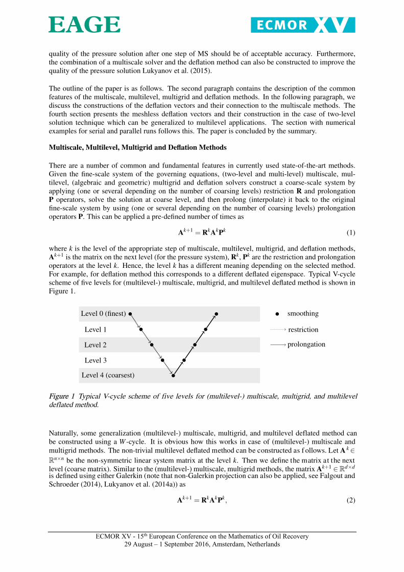
where k is the level of the appropriate step of multiscale, multilevel, multigrid, and deflation methods,Ak+1 is the matrix on the next level (for the pressure system), Rk, Pk are the restriction and prolongationoperators at the level k. Hence, the level k has a different meaning depending on the selected method.For example, for deflation method this corresponds to a different deflated eigenspace. Typical V-cyclescheme of five levels for (multilevel-) multiscale, multigrid, and multilevel deflated method is shown inFigure 1.

Level 0 (finest)

Level 1

Level 2

Level 3

Level 4 (coarsest)

smoothing

restriction

prolongation

Figure 1 Typical V-cycle scheme of five levels for (multilevel-) multiscale, multigrid, and multilevel deflated method.

Naturally, some generalization (multilevel-) multiscale, multigrid, and multilevel deflated method can be constructed using a W -cycle. It is obvious how this works in case of (multilevel-) multiscale and multigrid methods. The non-trivial multilevel deflated method can be constructed as f ollows. Let A k ∈ Rn×n be the non-symmetric linear system matrix at the level k. Then we define the matrix at the next level (coarse matrix). Similar to the (multilevel-) multiscale, multigrid methods, the matrix Ak+1 ∈ Rd×d

is defined using either Galerkin (note that non-Galerkin projection can also be applied, see Falgout and Schroeder (2014), Lukyanov et al. (2014a)) as

Ak+1 = RkAkPk, (2)

ECMOR XV - 15th European Conference on the Mathematics of Oil Recovery 29 August – 1 September 2016, Amsterdam, Netherlands

and the deflation matrices at the level k (i.e., Dk1 and Dk

2) are defined as

Dk1 = I−AkPk

(Ak+1

)−1Rk,

Dk2 = I−Pk

(Ak+1

)−1RkAk.

(3)

where A1 = A is the original fine scale matrix. The(Ak+1

)−1 is constructed to avoid a direct inversion

of the matrix and expensive matrix-matrix product in the expression(Ak+1

)−1 Rk. This is achievedby doing an user defined number pre- and a post-smoothing (e.g., Gauss-Seidel (GS) or ILU(0)) stepssimilar to Multigrid Solver (see, Lukyanov et al. (2014b)). Finally, the solution to the original linearsystem can be found using the relation:

x =k

∑i=1

Pi (Ai+1)−1(Ri)T b+

k

∏i=1

Di2x (4)

where x is a solution of the ’deflated system’:

k

∏i=1

Di1Ax =

k

∏i=1

Di1b (5)

The prolongation Pi and restriction Ri operators in deflation method are defined using the deflationmatrix, Zi (by no limiting example) as follows

Pi = Zi, Ri =(Zi)T

(6)

where Zi is the the deflation matrix between levels i and i + 1. Let us recall that the prolongationoperator P in multiscale methods such as the multiscale finite element (MSFE) and multiscale finitevolume (MSFV) are constructed based on local solutions (basis functions) of the fine-scale problem withdifferent boundary conditions. The local support for the basis functions are obtained by first imposing acoarse grid (Ωk) on the given fine-grid cells. The coarse grid operator is then constructed using Galerkincondition (1). The restriction operator, i.e., mapping fine scale to coarse scale, can be obtained by usingeither a finite element (MSFE) or finite volume (MSFV) methods as per terminology of the reservoirsimulation community. The former employs a transpose of the prolongation operator, i.e.,

RFE = PT , (7)

There is a clear similarity in constructing a coarse system between multiscale (MSFE, MSFV) and defla-tion method. The high-frequency errors at the fine scale in multiscale (MSFE, MSFV) are then resolvedby employing a smoother on fine grid. The equivalent step in deflation method is the solution of the’deflated system’ defined by the equation (5). It is clear that direct solution step of the ’deflated sys-tem’ can be substituted by performing smoothing iterations using either the original matrix A or deflatedmatrix

(∏

ki=1 Dk

1A). Hence, the primary difference between (two-level or multi-level) multiscale and

(two-level or multi-level) deflation method is the selection of the restriction and prolongation operators.Multiscale methods have been developed to describe local heterogeneities within the sub-domains in thecoarse system by using purely locally-supported basis functions. The deflation methods use a differentstrategy in constructing the restriction and prolongation operators based on the detailed analysis of theunderlying spectrum of the preconditioned matrix.

In recent years, the multiscale restriction smoothed basis (MsRSB) method was introduced (see, Møynerand Lie (2016)) to overcome the geological complexities and the use of complex grid geometries re-quired to compute compute the underlying basis functions. Below, it will be shown that the basis func-tions employed by MsRSB method have been extensively used in the deflation methods for variousapplications Tang and Vuik (2007a), Tang and Vuik (2007c), Tang and Vuik (2007b), Frank and Vuik(2001), Vuik et al. (2002), van der Linden et al. (2016)

ECMOR XV - 15th European Conference on the Mathematics of Oil Recovery 29 August – 1 September 2016, Amsterdam, Netherlands

Z0

Figure 2 Subdomain (a), levelset (b) and subdomain-levelset deflation (c).

Multiscale Restriction Smoothed Basis and Deflation Vectors

In both methods (i.e., MsRSB and Deflation), the discretized computational domain Ω is first decom-posed into d non-overlapping subdomains Ω j with j ∈ 1, . . . ,d. The deflation v ector j f orms j-th column of the deflation operator Z or initial basis functions P j of MsRSB method, corresponding t o Ω jand it is defined as (see, Frank and Vuik (2001), Tang (2008b), van der Linden (2013), van der Linden et al. (2016), Møyner and Lie (2016), Shah et al. (2016))

(P0

j)

i= (Z j)i =

1, xi ∈ Ω j

0, xi ∈Ω\ Ω j,(8)

where x j is a fine-scale grid cell center. Based on the above definition, Z j and P0j are piecewise-

constant vectors or functions (equal to a constant value of one inside the corresponding coarse domainΩ j), disjoint and orthogonal. For this choice of the deflation subspace, the deflation projectors P1 andP2 essentially agglomerate each subdomain in a single cell. Hence, the subdomain deflation and MsRSBare closely related to domain-decomposition methods and multigrid (see, Frank and Vuik (2001)). Forproblems in the bubbly flow, the span of the deflation vectors (8) approximates the span of the eigenvec-tors corresponding to the smallest eigenvalues Tang and Vuik (2007c). In our case, as studied by Vuiket al. (2002), the subdomains can be defined using the underlying heterogeneity, e.g., a low-permeableregion can be separated from the high-permeable regions and form d decompositions. As it was notedin Vermolen et al. (2004), it is better to use no overlap subdomains. This fact leads to the weightedoverlap method, which mimics average and no overlap in the case of no contrasts and large contrasts,respectively. It is shown that the overlap is crucial in approximating the eigenvectors corresponding tothe extreme eigenvalues.

In highly heterogeneous computational domain with large jumps in the permeability field, the subdomain-levelset deflation can be used (see, Tang and Vuik (2007c)). In this case where subdomain deflation doesnot take jumps into account, the subdomain-levelset deflation identifies different regions in the domainwith similar properties. A simple example is given in Figure 2. The fine grid is 12×14 with the coarsegrid 2×2 are shown in Figure 2. In each case, the values shown on the fine cells correspond to the valuesin the first deflation vector. In the middle and right figure, the border between the yellow circles (highpermeability) and white circles (low permeability) exemplifies a sharp contrast in the matrix coefficient.The figures shows the following:

• In the left figure, subdomain deflation is used. The red solid line divides the domain into the foursubdomains Ω1,Ω2,Ω3 and Ω4. Each subdomain corresponds to a unique deflation vector.

• In the middle figure, levelset deflation is used. This time, the red solid line coincides with thecontrast in the matrix coefficient. As a result, we get the two domains Ω1 and Ω2.

ECMOR XV - 15th European Conference on the Mathematics of Oil Recovery 29 August – 1 September 2016, Amsterdam, Netherlands

• In the right figure, subdomain-levelset deflation is used. The subdomain division is determinedusing certain criteria, which in this example leads to the division red solid line between Ω1 andΩ2. Within each subdomain, levelset deflation uses the jump between the high permeability andlow permeability cells to obtain the subdomains Ω1,Ω2,Ω3 and Ω4.

In this paper, the subdomain-levelset deflation concept is used. We highlight the fact that the algorithmis particularly suitable for a parallel implementation. We can apply the levelset deflation method toeach subdomain (coarse cells), and append the deflation vectors with zeros for all cells outside theneighboring subdomains. Furthermore, it is important to note that deflation vectors can be constructedbased on the jump in the PVT data (e.g., bubbly flow Tang and Vuik (2007c)). For example, duringthe polymer flooding the aqueous viscosity changes drastically in the presence of polymer. Hence, thedeflation vectors can be constructed based on the location of the polymer with in the reservoir.

Although we have identify a full analogy between deflated vectors Z and initial basis functions P0j of

MsRSB method, the final restriction-smoothed basis functions are computed by employing a modifiedform of the damped-Jacobi smoothing approach:

δPη

k =−ωD−1APη

k (9)

where A is the fine-scale matrix, D = diag(A) is the diagonal part of the matrix A. The final update forprolongation operator is defined as

Pη+1k = Pη

k +δPη

k (10)

where δPη

k is the restricted iterative increments (see, Møyner and Lie (2016), Shah et al. (2016)). Toensure that basis functions have local support, the increments δPη

k is restricted to have nonzero valuesonly inside Ωk leading to the definition of the δPk. Finally, the the basis functions (9)-(10) of theMsRSB method can be written in the abstract form as:

Pk = M12MsRBSP

0k (11)

where M12MsRBS is the predefined smoothing matrix of MsRBS method defined by (9)-(10) and restriction

expression (see, Møyner and Lie (2016), Shah et al. (2016)).

Remarks

• The proposed method is similar to smoothed aggregation-based multigrid methods (see, Vanek(1992), Vanek et al. (1996))

• A deflation technique applied to a preconditioned system with preconditioner M−1 at differentlevel k

Dk1 = I− AkPk

(Ak+1

)−1Rk, Dk

2 = I− Pk(

Ak+1)−1

RkAk,

Ai+1 = RiAiPi, Pi = Zi, Ri =(Zi)T

, Z = M−12 Z

(12)

is equivalent to preconditioning of a deflated system

k

∏i=1

Di1M−1Ax =

k

∏i=1

Di1M−1b, x =

k

∑i=1

Pi(

Ai+1)−1

(Ri)T (M−1b)+k

∏i=1

Di2x (13)

Here Ai+1 =i

∏l=1

Rl(M−1A)Pl , ˆx is a solution of the preconditioned ’deflated system’. The matrix

Z is interpreted as a preconditioned deflation-subspace matrix (see, Tang (2008b) who formulatedthis for a two-level deflation method applied to symmetric positive definite matrix):

Z = M12 Z (14)

ECMOR XV - 15th European Conference on the Mathematics of Oil Recovery 29 August – 1 September 2016, Amsterdam, Netherlands

where M is the specified preconditioner. Comparison of the equation (14) with the equation(11) and taking into account that P0

j = Z j leads to the fact that two-level (preconditioned with the

matrix M12MsRBS) deflation projection with the post smoothing used in MsRBS should give identical

results with MsRBS. Commonly, the deflation matrix (matrix of basis functions) Z is applied topreconditioned matrix M−1A and, hence, the smoothing (14) is not applied since it is equivalentto have twice preconditioning of the matrix A.

• Localization can be constructed using any partition of unity (PU) functions ϕi with Ωi =supp(ϕi) at any level k as follows

p =N

∑i=1

ϕi pi =N

∑i=1

(ϕi pi

smooth +ϕi pijump +ϕi pi

singular

)(15)

where pismooth is the smooth part of the solution, pi

singular is the part of the solution with singularity,pi

jump is the part of the solution with the jumps, and functions ϕi play the role of “glue”.

Meshless Deflation Vectors

The meshless deflation vectors (basis functions) utilize some advantages of the existing multiscaleschemes and meshless methods. In light of this, the meshless deflation vectors (basis functions) areconstructed using two sets of computational points (see, Lukyanov et al. (2014b)):

1. Fine points set SF (e.g., cell centers of underlying mesh), i.e. Ω = span

ΩXI ,h/I = 1, ...,NF

consisting of NF patches which are interior to the support of the kernel W(X−XI, h

), i.e. ΩX,h =

suppW (X−ξ , h), NF is the number of points, hF is the fine scale diameter (or smoothing length);

2. Coarse points set SC (e.g., user defined points), i.e. Ω = span

ΩXJ ,h/J = 1, ...,NC

consisting ofNC patches which are interior to the support of the kernel W (XI−X,h), i.e. ΩX,h = suppW (X−ξ ,h), NC < NF is the number of points, hC is the coarse scale diameter (or smoothing length);

In both cases (fine and coarse), the same cubic spline for kernel function W was used (see, Lukyanovet al. (2014b)). Following the conventional multiscale approach, the approximation of the fine scalepressure distribution pF using coarse set values pC is constructed as

pF (X)≈NC

∑J=1

VξJ ·W (X−ξJ,hC) · pC (ξJ) (16)

or

pF (XI)≈

XI ·

(NC

∑J=1

VξJ ·W (XI−ξJ,hC)

[NC

∑K=1

[pC (ξK)− pC (ξJ)]∇∗W (ξJ−ξK ,hC)

])+

+NC

∑J=1

[VξJ ·W (XI−ξJ,hC) ·

(pC (ξJ)−ξJ ·

(NC

∑K=1

[pC (ξK)− pC (ξJ)]∇∗W (ξJ−ξK ,hC)

))] (17)

The scheme (17) provides a first-order consistent prolongation from a coarse set of particles into a fineset of particles, i.e. it provides an exact solution for a linear pressure distribution at both scales. Incase where coarse level points do not form a subset of fine level points, the aggressive restriction is alsoapplied following relations (zero and first-order consistent operators) such as:

pC (X)≈NF

∑J=1

VξJ ·W (X−ξJ,hF) · pF (ξJ) (18)

ECMOR XV - 15th European Conference on the Mathematics of Oil Recovery 29 August – 1 September 2016, Amsterdam, Netherlands

or

pC(XI)≈ XI ·

(NF

∑J=1

VξJ ·W (XI−ξJ,hF)

[NF

∑K=1

[pF(ξK)− pF(ξJ)]∇∗W (ξJ−ξK ,hF)

])+

+NF

∑J=1

[VξJ ·W (XI−ξJ,hF) ·

(pF (ξJ)−ξJ ·

(NF

∑K=1

[pF(ξK)− pF(ξJ)]∇∗W (ξJ−ξK ,hF)

))] (19)

It is important to note that relations (16), (17), (18), (19) can be written using matrix notation:

uF = WP ·uC, WP : SC→ SF uC = WR ·uF , WR : SF → SC˜WR= B−1

W WR, BW = WRWP, ˜WRWP = I, ˜WR

: SF → SC˜WP= WPB−1

W , BW = WRWP, WR˜WP= I, ˜WP

: SC→ SF

(20)

where WP and ˜WPare the prolongation operators, WR and ˜WR

are the restriction operators. In general,it is clear that WR 6=

(WP)T . As a result, the following options are available to construct deflation

vectors for restriction and prolongation operators:

(I) P = WP, R =(WP)T

, (II) P = ˜WP, R =

(˜WP)T

(III) P = WP, R = WR, (IV ) P = WP, R = ˜WR, (V ) P = ˜WP

, R = WR

(V I) P =(WR)T

, R = WR, (V II) P =

(˜WR)T

, R = ˜WR

The option (I) is used in this paper. The prolongation and restriction operators in this method are basedon a SPH gradient approximation (instead of solving localized flow problems) commonly used in themeshless community for thermal, viscous, and pressure projection problems. Furthermore, the smooth-ing length hC can be selected to maintain only the host particle in the compact support resulting in thebasis functions defined by the equation (8). Hence, the meshless basis functions provide a more flexibleframework for constructing deflation vectors (or basis functions).

Multiscale Meshless Based Method

The linear system of equations (primary focus is the pressure equations) with the matrix AF and righthand side bF can be difficult to solve, if its condition number k = ‖AF‖

∥∥A−1F

∥∥ is large. This motivatesthe concept of preconditioning. Let V be an approximation of A−1, which is easy to construct and tosolve for a given input. Hence, we can write a simple Richardson iteration scheme with the predefinednumber of application of the multilevel multiscale meshless based preconditioner:

[pF ]m+1 = [pF ]

m +V · (bF −AF [pF ]m) (21)

where m is the iteration index, (pF)m is the pressure vector at the iteration m, V is the left multiscale

meshless based preconditioner defined as an operational object. A meshless multiscale preconditioner isconstructed as follows for a given input vF and output zF using a two-level case by no limiting example:

[zF ] = P(AC)−1 R [vF ] , AC = RAFP (22)

[wF ] = [zF ]+S−1γ · ([vF ]−AF [zF ]) (23)

where S−1γ is the smoothing operator (e.g., Gauss-Seidel (GS) or ILU(k) or BILU(k) smoothing method

or Krylov-space accelerator) applied γ times. The multiscale meshless based method involves setting upthe restriction and prolongation operators, which can be constructed at the beginning of the simulations.

The coarse pressure system ACv = w can be solved with different strategies depending on the size of thecoarse pressure matrix. The size of the coarse pressure matrix is defined by the size of the model andthe choice of the coarsening factors. If the size of the coarse system is small a direct solver can be used.The iterative methods are used for the large coarse system.

ECMOR XV - 15th European Conference on the Mathematics of Oil Recovery 29 August – 1 September 2016, Amsterdam, Netherlands

Numerical Experiments

In this section, the performance results of the fully implicit smoothed particle hydrodynamics (meshless)based multiscale method (MsMBM) are presented. The method has been prototyped in a commercialreservoir simulator and the method was compared against the two stage CPR-AMG-ILU(0) solver, whichis the default solution strategy in majority of commercial simulators.

The test cases are classified by the number of grid cells, fluid models and time discretization. Thefollowing characteristics were compared between the default and proposed solutions.

• Time steps: the total number of time steps required to complete the simulation.

• Non-linear iterations: the number of non-linear iterations in the simulation.

• Linear iterations: the number of iterations used to solve the linear systems generated by the non-linear solver.

• Linear solver time: the amount of time needed to solve the linear systems.

• CPU time: the overall computational time required to complete the simulation.

Test Cases

Table 1 describes all the running five test cases ranging from relatively small (not too small) models torelatively large (not too large) real life test cases. The black oil, iso-thermal and thermal compositional

Active cells Dimensions Fluid model ImplicitnessNumber of

Number of activephases components

389557 154×90×34 Compositional AIM IMPES 3 13Isothermal348807 238×192×114 Black Oil Isothermal Fully Implicit 3 3

348812 238×192×114 Compositional AIM IMPES 3 8Isothermal

1722781 18×1126×85 Compositional Thermal Fully Implicit 3 3with steam permitted

164945 not a ‘box’ Compositional Thermal Fully Implicit 3 3with steam permitted

Table 1 Basic properties of the simulated test cases.

models with varying degree of heterogeneity in the reservoir grid properties are considered in this paper to test the performance of the Multiscale Meshless Based Method (MsMBM). The names of the test cases correspond to the total number of cells in the models. Table 1 contains several examples where the number of active cells is lower than the number of cells suggested by the dimensions. In those cases, the domain includes a number of inactive cells. The settings for the simulation test cases can be found in Table 2, where the parameter k represents the number of the top level GMRES accelerations with MsMBM preconditioner. The following tables and figures shows the performance results for all experimental tests including reference performance results (CPR-AMG-ILU(0)).

In general, Multiscale Meshless Based Method (MsMBM) does not change the number of time steps and non-linear iterations compared to the CPR-AMG-ILU(0) solution strategy in the considered simulations. This is due to second stage preconditioner ILU(0), which eliminates all the differences in the pressure solver, where AMG and MsMBM are applied. However, in all cases there is a significant effect on the number of linear iterations. This is a very common observations for multiscale solutions strategies (see,

ECMOR XV - 15th European Conference on the Mathematics of Oil Recovery 29 August – 1 September 2016, Amsterdam, Netherlands

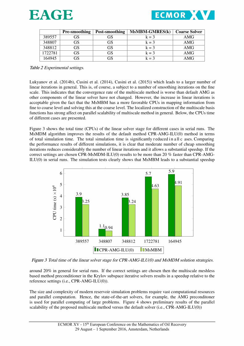
Pre-smoothing Post-smoothing MsMBM-GMRES(k) Coarse Solver389557 GS GS k = 3 AMG348807 GS GS k = 3 AMG348812 GS GS k = 3 AMG1722781 GS GS k = 3 AMG164945 GS GS k = 3 AMG

Table 2 Experimental settings.

Lukyanov et al. (2014b), Cusini et al. (2014), Cusini et al. (2015)) which leads to a larger number of linear iterations in general. This is, of course, a subject to a number of smoothing iterations on the fine scale. This indicates that the convergence rate of the multiscale method is worse than default AMG as other components of the linear solver have not changed. However, the increase in linear iterations is acceptable given the fact that the MsMBM has a more favorable CPUs in mapping information from fine to coarse level and solving this at the coarse level. The localized construction of the multiscale basis functions has strong affect on parallel scalability of multiscale method in general. Below, the CPUs time of different cases are presented.

Figure 3 shows the total time (CPUs) of the linear solver stage for different cases in serial runs. The MsMDM algorithm improves the results of the default method CPR-AMG-ILU(0) method in terms of total simulation time. The total simulation time is significantly r educed i n a ll c ases. Comparing the performance results of different simulations, it is clear that moderate number of cheap smoothing iterations reduces considerably the number of linear iterations and it allows a substantial speedup. If the correct settings are chosen CPR-MsMDM-ILU(0) results to be more than 20 % faster than CPR-AMG-ILU(0) in serial runs. The simulation tests clearly shows that MsMBM leads to a substantial speedup

389557 348807 348812 1722781 164945

1

2

3

4

5

6

3.9

1.1

3.85

5.7 5.9

3.25

0.94

3.24

4.634.91

CPU

time

(s)×

104

CPR-AMG-ILU(0) MsMBM

Figure 3 Total time of the linear solver stage for CPR-AMG-ILU(0) and MsMDM solution strategies.

around 20% in general for serial runs. If the correct settings are chosen then the multiscale meshless based method preconditioner in the Krylov subspace iterative solvers results in a speedup relative to the reference settings (i.e., CPR-AMG-ILU(0)).

The size and complexity of modern reservoir simulation problems require vast computational resources and parallel computation. Hence, the state-of-the-art solvers, for example, the AMG preconditoner is used for parallel computing of large problems. Figure 4 shows preliminary results of the parallel scalability of the proposed multiscale method versus the default solver (i.e., CPR-AMG-ILU(0))

ECMOR XV - 15th European Conference on the Mathematics of Oil Recovery 29 August – 1 September 2016, Amsterdam, Netherlands

4 8 16 320.5

1

1.5

2

2.5 2.4

1.6

0.95 0.88

2.1

1.31

0.780.65

CPU

time

(s)×

104

CPR-AMG-ILU(0) MsMBM

Figure 4 Scalability of the total time of the simulation runs for CPR-AMG-ILU(0) and MsMDM solu-tion strategies in the case 389557.

It is clear that further analysis of the method and its scalability is required to obtain full picture about capabilities of the proposed method.

Conclusions

A preconditioned Krylov subspace method such as the preconditioned FGMRES method can signif-icantly improve the convergence and robustness of a numerical simulator. This paper considers the preconditioned GMRES method with multilevel multiscale meshless based method for solving such pressure system. The solution technique proposed in this paper uses a meshless approximation method to construct a priori the deflation space (or basis functions s pace). The analysis of the common funda-mental features of different multiscale strategies are presented.

In this paper, a parallel fully implicit smoothed particle hydrodynamics (SPH) based multiscale method for solving pressure system is presented. The prolongation and restriction operators in this method are based on a SPH gradient approximation (instead of solving localized flow problems) commonly used in the meshless community for thermal, viscous, and pressure projection problems. This method can reduce to the recently proposed MsRSB. In general, it gives more flexibility i n c onstructing various restriction and prolongation operators.

This method has been prototyped in a commercially available simulator. This method does not require a coarse partition and, hence, can be applied to general unstructured topology of the fine s cale. The SPH (or meshless) based multiscale method provides a reasonably good approximation to the pressure system and speeds up the convergence when used as a preconditioner for an iterative fine-scale solver. In addition, it exhibits expected good scalability during parallel simulations. Presented numerical results support theoretical and practical expectations from this method. Additional analysis of this method is required to identify the optimal parameters of this method.

ECMOR XV - 15th European Conference on the Mathematics of Oil Recovery

29 August – 1 September 2016, Amsterdam, Netherlands

References

Cao, H., Tchelepi, H., Wallis, J. and Yardumian, H. [2005] Constrained Residual Acceleration of Con-jugate Residual Methods. SPE Annual Technical Conference and Exhibition.

Cortinovis, D. and Jenny, P. [2014] Iterative Galerkin-Enriched Multiscale Finite-Volume Method. J.Comp. Phys., 277, 248–267.

Cusini, M., Lukyanov, A., Natvig, J. and Hajibeygi, H. [2014] A Constrained Pressure Residual Multi-scale (CPR-MS) Compositional Solver. ECMOR XIV - 14th European Conference on the Mathematicsof Oil Recovery, EAGE.

Cusini, M., Lukyanov, A., Natvig, J. and Hajibeygi, H. [2015] Constrained Pressure Residual Multiscale(CPR-MS) Method. Journal of Computational Physics, 299, 472–486.

Dostál, Z. [1988] Conjugate gradient method with preconditioning by projector. International Journalof Computer Mathematics, 23(3-4), 315–323.

Efendiev, Y. and Hou, T. [2009] Multiscale Finite Element Methods: Theory and Applications. Springer.Falgout, R. and Schroeder, J. [2014] Non-Galerkin Coarse Grids for Algebraic Mutigrid. SIAM Journal

on Scientific Computing, 36(3), 309–334.Frank, J. and Vuik, C. [2001] On the construction of deflation-based preconditioners. SIAM J. Sci.

Comput., 23(2), 442–462.Hajibeygi, H., Bonfigli, G., Hesse, M. and Jenny, P. [2008] Iterative multiscale finite-volume method. J.

Comput. Phys., 227, 8604–8621.Hou, T. and Wu, X.H. [1997] A multiscale finite element method for elliptic problems in composite

materials and porous media. J. Comput. Phys., 134, 169–189.Jenny, P., Lee, S. and Tchelepi, H. [2003] Multiscale finite-volume method for elliptic problems in

subsurface flow simulation. J. Comput. Phys., 187, 47–67.Jönsthövel, T., van Gijzen, M., MacLachlan, S., Scarpas, A. and Vuik, C. [2011] Comparison of the

deflated preconditioned conjugate gradient method and algebraic multigrid for composite materials.Computational Mechanics, 1–13.

Jönsthövel, T., van Gijzen, M., Vuik, C., Kasbergen, C. and Scarpas, A. [2009] Preconditioned conjugategradient method enhanced by deflation of rigid body modes applied to composite materials. ComputerModeling in Engineering and Sciences, 47, 97–118.

Klie, H., Wheeler, M., Stueben, K. and Clees, T. [2007] Deflation AMG solvers forhighly ill-conditioned reservoir simulation problems. SPE Reservoir Simulation Symposium,doi:10.2118/105820-MS.

Kozlova, A., Li, Z., Natvig, J., Watanabe, S., Zhou, Y., Bratvedt, K., and Lee, S. [2015] A real-field Mul-tiscale Black-Oil Reservoir Simulator. SPE Reservoir Simulation Symposium, Society of PetroleumEngineers, Houston, Texas, USA.

van der Linden, J. [2013] Development of a deflation-based linear solver in petroleum reservoir simula-tion. Msc Thesis TU Delft.

van der Linden, J., Jönsthövel, T., Lukyanov, A. and Vuik, C. [2016] The parallel subdomain-levelsetdeflation method in reservoir simulation. Journal of Computational Physics, 304, 340–358.

Lukyanov, A., Hajibeygi, H., Natvig, J. and Bratvedt, K. [2014a] A multilevel Galerkin and Non-Galerkin, conditionally and Unconditionally Monotone Constrained Pressure Residual MultiscaleMethods. US Patent Docket No.: IS14.8805.

Lukyanov, A., Hajibeygi, H., Vuik, C. and Bratvedt, K. [2015] Adaptive Deflated Multiscale Solver. USPatent Docket No. IS14.9739-US-PSP.

Lukyanov, A., van der Linden, J., Jonsthovel, T. and Vuik, C. [2014b] Meshless Subdomain DeflationVectors in the Preconditioned Krylov Subspace Iterative Solvers. ECMOR XIV - 14th EuropeanConference on the Mathematics of Oil Recovery, EAGE.

Lunati, I. and Jenny, P. [2006] Multiscale finite-volume method for compressible multiphase flow inporous media. Journal of Computational Physics, 216(2), 616–636.

Lunati, I., Tyagi, M. and Lee, S. [2011] An iterative multiscale finite volume algorithm converging tothe exact solution. Journal of Computational Physics, 230(5), 1849–1864.

Manea, A., Sewall, J. and Tchelepi, H. [2015] Parallel multiscale Linear Solver for Highly DetailedReservoir Models. SPE Reservoir Simulation Symposium, Society of Petroleum Engineers, Houston,Texas, USA.

ECMOR XV - 15th European Conference on the Mathematics of Oil Recovery 29 August – 1 September 2016, Amsterdam, Netherlands

Møyner, O. and Lie, K. [2016] A Multiscale Restriction-Smoothed Basis Method for High ContrastPorous Media Represented on Unstructured Grids. Journal of Computational Physics, 304, 46–71.

Nicolaides, R. [1987] Deflation of Conjugate Gradients with Applications to Boundary Value Problems.SIAM J. Numer. Anal., 24(2), 355–365.

Ruge, J. and Stuben, K. [1987] Algebraic multigrid (AMG). In: McCormick, S. (Ed.) Multigrid Meth-ods, 3, SIAM, Philadelphia, PA, 73–130.

Saad, Y. and Schultz, M. [1986] A generalized minimal residual algorithm for solving nonsymmetriclinear systems. SIAM J. Sci. Stat. Comput., 7(3), 856–869.

Shah, S., MÃÿyner, O., Tene, M., Lie, K.A. and Hajibeygi, H. [2016] The multiscale restrictionsmoothed basis method for fractured porous media (F-MsRSB). Journal of Computational Physics,318, 36–57.

Tang, J. [2008a] Two-Level preconditioned conjugate gradient methods with applications to bubbly flowproblems. PhD Thesis TU Delft.

Tang, J. [2008b] Two-Level Preconditioned Conjugate Gradient Methods with Applications to BubblyFlow Problems. PhD Thesis TU Delft.

Tang, J. and Vuik, C. [2007a] Acceleration of Preconditioned Krylov Solvers for Bubbly Flow Problems.In: Shi, Y., Albada, G., Dongarra, J. and Sloot, P. (Eds.) Computational Science - ICCS 2007, LectureNotes in Computer Science, 4487, Springer Berlin Heidelberg, 874–881.

Tang, J. and Vuik, C. [2007b] Efficient deflation methods applied to 3-D bubbly flow problems. Elec-tronic Transactions on Numerical Analysis, 26, 330–349.

Tang, J. and Vuik, C. [2007c] New variants of deflation techniques for pressure correction in bubblyflow problems. Journal of Numerical Analysis, Industrial and Applied Mathematics, 2, 227–249.

Tene, M., Hajibeygi, H. and Y. Wang, H.T. [2014] Compressible Algebraic Multiscale Solver (CAMS).Proceedings of the 14th European Conference on the Mathematics of Oil Recovery (ECMOR), Cata-nia, Sicily, Italy.

Vanek, P. [1992] Acceleration of convergence of a two-level algorithm by smoothing transfer operator.Appl. Math., 37, 265–274.

Vanek, P., Mandel, J. and Brezina, M. [1996] Algebraic multigrid by smoothed aggregation for secondand fourth order eliptic problems. Computing, 56(2), 179–196.

Vermolen, F., Vuik, C. and Segal, A. [2004] Deflation in preconditioned conjugate gradient methodsfor finite element problems. In M. Krizek, P. Neittaanmäki, R. Glowinski, and S. Korotov, editors,Conjugate Gradient and Finite Element Methods. Springer, Berlin, 2004, 103–129.

Vuik, C., Segal, A., el Yaakoubi, L. and Dufour, E. [2002] A Comparison of Various Deflation VectorsApplied to Elliptic Problems with Discontinuous Coefficients. Appl. Numer. Math., 41(1), 219–233.

Wallis, J. [1983] Incomplete Gaussian Elimination as a Preconditioning for Generalized Conjugate Gra-dient Acceleration. SPE Reservoir Simulation Symposium, Society of Petroleum Engineers, Houston,Texas, USA.

Wallis, J. [1985] Constrained residual acceleration of conjugate residual methods. SPE Reservoir Simu-lation Symposium, (1), doi:10.2118/13536–MS.

Wang, Y., Hajibeygi, H. and Tchelepi, H. [2014] Algebraic multiscale solver for flow in heterogeneousporous media. Journal of Computational Physics, 259, 284–303.

Zhou, H. and Tchelepi, H. [2012] Two-stage algebraic multiscale linear solver for highly heterogeneousreservoir models. SPE Journal, 17(2), 523–539.