Parallel Evidence Propagation on Multicore Processorshalcyon.usc.edu/~pk/prasannawebsite/papers/xia09pact.pdf · Parallel Evidence Propagation on Multicore ... applications in a number

Parallel Evidence Propagation on Multicore

Processors⋆

Yinglong Xia1, Xiaojun Feng3 and Viktor K. Prasanna2,1

Computer Science Department1 and Department of Electrical Engineering2

University of Southern California, Los Angeles, CA 90089, U.S.A.Department of Computer Science and Technology3

Tsinghua University, Beijing 100084, China{yinglonx, prasanna}@usc.edu, [email protected]

Abstract. In this paper, we design and implement an efficient techniquefor parallel evidence propagation on state-of-the-art multicore proces-sor systems. Evidence propagation is a major step in exact inference, akey problem in exploring probabilistic graphical models. We propose arerooting algorithm to minimize the critical path in evidence propaga-tion. The rerooted junction tree is used to construct a directed acyclicgraph (DAG) where each node represents a computation task for evi-dence propagation. We develop a collaborative scheduler to dynamicallyallocate the tasks to the cores of the processors. In addition, we integratea task partitioning module in the scheduler to partition large tasks so asto achieve load balance across the cores. We implemented the proposedmethod using Pthreads on both AMD and Intel quadcore processors. Fora representative set of junction trees, our method achieved almost linearspeedup. The execution time of our method was around twice as fast asthe OpenMP based implementation on both the platforms.

Key words: Exact inference, Multicore, Junction tree, Scheduling

1 Introduction

A full joint probability distribution for any real-world system can be used forinference. However, such a distribution increases intractably with the number ofvariables used to model the system. It is known that independence and condi-tional independence relationships can greatly reduce the size of the joint proba-bility distributions. This property is utilized by Bayesian networks [1]. Bayesiannetworks have been used in artificial intelligence since the 1960s. They have foundapplications in a number of domains, including medical diagnosis, consumer helpdesks, pattern recognition, credit assessment, data mining and genetics [2][3][4].

Inference in a Bayesian network is the computation of the conditional prob-ability of the query variables, given a set of evidence variables as the knowledge

⋆ This research was partially supported by the U.S. National Science Foundation un-der grant number CNS-0613376. NSF equipment grant CNS-0454407 is gratefullyacknowledged.

1

2 Y. Xia, X. Feng, and V. Prasanna

to the network. Inference in a Bayesian network can be exact or approximate.Exact inference is NP hard [5]. The most popular exact inference algorithm formultiply connected networks was proposed by Lauritzen and Speigelhalter [1],which converts a Bayesian network into a junction tree, then performs exactinference in the junction tree. The complexity of exact inference algorithms in-creases dramatically with the density of the network, the width of the cliquesand the number of states of the random variables in the cliques. In many casesexact inference must be performed in real time.

Almost all recent processors are designed to process simultaneous threads toachieve higher performance than single core processors. Typical examples of mul-ticore processors available today include AMD Opteron and Intel Xeon. Whilechip multi-processing has been devised to deliver increased performance, an im-portant challenge is to exploit the available parallelism. Prior work has shownthat system performance is sensitive to thread scheduling in simultaneous mul-tithreaded (SMT) architectures [6]. To maximize the potential of such multicoreprocessors, users must understand both the algorithmic and architectural aspectsto design efficient scheduling solutions.

In this paper, we study parallelization of evidence propagation on state-of-the-art multicore processors. We exploit both structural parallelism and dataparallelism to improve the performance of evidence propagation. We achievedspeedup of 7.4 using 8 cores on state-of-the-art platforms. This speedup is muchhigher compared with the baseline methods e.g. OpenMP based implementation.The proposed method can be extended for online scheduling of directed acyclicgraph (DAG) structured computations.

The paper is organized as follows: In Section 2, we discuss the background ofevidence propagation. Section 3 introduces related work. In Section 4, we presentjunction tree rerooting. Section 5 defines computation tasks for evidence prop-agation. Section 6 presents our collaborative scheduler for multicore processors.Experimental results are shown in Section 7. Section 8 concludes the paper.

2 Background

A Bayesian network is a probabilistic graphical model that exploits conditionalindependence to represent compactly a joint distribution. Figure 1 (a) showsa sample Bayesian network, where each node represents a random variable.The edges indicate the probabilistic dependence relationships between two ran-dom variables. Notice that these edges can not form directed cycles. Thus, thestructure of a Bayesian network is a directed acyclic graph (DAG), denotedG = (V, E), where V = {A1, A2, . . . , An} is the node set and E is the edge set.Each random variable in the Bayesian network has a conditional probability table

P (Aj |pa(Aj)), where pa(Aj) is the parents of Aj . Given the Bayesian network,a joint distribution is given by P (V) =

∏n

j=1 P (Aj |pa(Aj)), where Aj ∈ V [1].The evidence in a Bayesian network is the variables that have been instan-

tiated, e.g. E = {Ae1= ae1

, · · · , Aec= aec

}, ek ∈ {1, 2, . . . , n}, where Aeiis a

variable and aeiis the instantiated value. Evidence can be propagated to other

Parallel Evidence Propagation on Multicore Processors 3

variables in the Bayesian network using Bayes’ Theorem. Propagating the evi-dence throughout a Bayesian network is called inference, which can be exact orapproximate. Exact inference is proven to be NP hard [5]. The computationalcomplexity of exact inference increases dramatically with the size of the Bayesiannetwork and the number of states of the random variables.

Traditional exact inference using Bayes’ theorem fails for networks with undi-rected cycles [1]. Most inference methods for networks with undirected cyclesconvert a network to a cycle-free hypergraph called a junction tree. We illus-trate a junction tree converted from the Bayesian network (Figure 1 (a)) inFigure 1 (b), where all undirected cycles in are eliminated. Each vertex in Fig-ure 1 (b) contains multiple random variables from the Bayesian network. For thesake of exploring evidence propagation in a junction tree, we use the followingnotations to formulate a junction tree. A junction tree is defined as J = (T, P̂),

where T represents a tree and P̂ denotes the parameter of the tree. Each vertexCi, known as a clique of J, is a set of random variables. Assuming Ci and Cj are

adjacent, the separator between them is defined as Ci ∩Cj . P̂ is a set of potential

tables. The potential table of Ci, denoted ψCi, can be viewed as the joint distri-

bution of the random variables in Ci. For a clique with w variables, each havingr states, the number of entries in Ci is rw.

Fig. 1. (a) A sample Bayesian network and (b) corresponding junction tree.

In a junction tree, exact inference proceeds as follows: Assuming evidence isE = {Ai = a} and Ai ∈ CY , E is absorbed at CY by instantiating the variableAi and renormalizing the remaining variables of the clique. The evidence is thenpropagated from CY to any adjacent cliques CX . Let ψ∗

Y denote the potential tableof CY after E is absorbed, and ψX the potential table of CX . Mathematically,evidence propagation is represented as [1]:

ψ∗S =

∑

Y\S

ψ∗Y , ψ∗

X = ψXψ∗S

ψS(1)


where S is a separator between cliques X and Y; ψS ( ψ∗S ) denotes the original

(updated) potential table of S; ψ∗X is the updated potential table of CX .

3 Related Work

There are several works on parallel exact inference, such as Pennock [5], Ko-zlov and Singh [7] and Szolovits. However, some of those methods, such as [7],are dependent upon the structure of the Bayesian network. The performanceis adversely affected if the structure of the input Bayesian network is changed.Our method can be used for Bayesian networks and junction trees with variousstructures. Some other methods, such as [5], exhibit limited performance for mul-tiple evidence inputs. The performance of our method does not depend on thenumber of evidence cliques. In [8], the authors discuss the structure conversionof Bayesian networks, which is different from evidence propagation addressedin this paper. In [9], the node level primitives are parallelized using messagepassing on distributed memory platforms. The optimization proposed in [9] isnot applicable in this paper, since the multicore platforms have shared mem-ory. However, the idea of parallelization of node level primitives is adapted byour scheduler to partition large tasks. A junction tree decomposition method isprovided in [10] to partition junction trees for distributed memory platforms.This method reduces communication between processors by duplicating somecliques. We do not apply junction tree decomposition on our multicore plat-forms, because the clique duplication consumes memory that is shared by all thecores. A centralized scheduler for exact inference is introduced in [11], which isimplemented on Cell BE, a heterogeneous multicore processor with a PowerPCelement and 8 computing elements. However, the multicore platforms studied inthis paper are homogeneous, and the number of cores is small. Using a separatecore for centralized scheduling leads to performance loss. We deviate from theabove approaches and explore collaborative task scheduling techniques for exactinference.

4 Junction Tree Rerooting For Minimizing Critical Path

A junction tree can be rerooted at any clique [5]. Consider rerooting a junctiontree at clique C. Let α be a preorder walk of the underlying undirected tree,starting from C. Then, α encodes the desired new edge directions, i.e. an edge inthe rerooted tree points from Cαi

to Cαjif and only if αi < αj . In the rerooting

procedure, we check the edges in the given junction tree and reverse any edgesinconsistent with α. The result is a new junction tree rooted at C, with the sameunderlying undirected topology as the original tree.

Rerooting a junction tree can lead to acceleration of evidence propagationon parallel computing systems. Let P (Ci, Cj) = Ci, Ci1 , Ci2 , ..., Cj denote a pathfrom Ci to Cj in a junction tree, and L(Ci,Cj) denote the weight of path P (Ci, Cj).Given clique width wCt

and clique degree kt for any clique Ct ∈ P (Ci, Cj), the


weight of the path L(Ci,Cj) is given by:

L(Ci,Cj) =∑

Ct∈P (Cr,Cj)

ktwCt

wCt∏

l=1

rl (2)

The critical path (CP) of a junction tree is defined as the longest weightedpath fin the junction tree. Give a junction tree J, the weight of a critical path,denoted LCP , is given by LCP = maxCj∈J L(Cr,Cj), where Cr is the root. Noticethat evidence propagation in a critical path takes at least as much time as that inother paths. Thus, among the rerooted junction trees, the one with the minimumcritical path leads to the best performance on parallel computing platforms.

A straightforward approach to find the optimal rerooted tree is as follows:First, reroot the junction tree at each clique. Then, for each rerooted tree, cal-culate the complexity of the critical path. Finally, select the rerooted tree corre-sponding to the minimum complexity of the critical path. Given the number ofcliques N and maximum clique width wC , the computational complexity of theabove procedure is O(N2wC).

We present an efficient rerooting method to minimize the critical path (seeAlgorithm 1), which is based on the following lemma:

Lemma 1: Suppose that P (Cx, Cy) is the longest weighted path from a leafclique Cx to another leaf clique Cy in a given junction tree, and L(Cr,Cx) ≥ L(Cr,Cy),where Cr is the root. Then, P (Cr, Cx) is a critical path in the given junction tree.

Proof sketch: Assume a critical path is P (Cr, Cz) where Cz 6= Cx. Let P (Cr, Cb1)denote the longest common segment between P (Cr, Cx) and P (Cr, Cy), and P (Cr, Cb2)the longest common segment between P (Cr, Cx) and P (Cr, Cz). Without lossof generality, assume Cb2 ∈ P (Cr, Cb1). Since P (Cr, Cz) is a critical path, wehave L(Cr,Cz) ≥ L(Cr,Cx). Because L(Cr,Cz) = L(Cr,Cb2) + L(Cb2,Cz) and L(Cr,Cx) =L(Cr,Cb2) + L(Cb2,Cb1) + L(Cb1,Cx), therefore, L(Cb2,Cz) ≥ L(Cb2,Cb1) + L(Cb1,Cx) >L(Cb1,Cx). Thus, we can find path P (Cz, Cy) = P (Cz, Cb2)P (Cb2, Cb1)P (Cb1, Cy)which leads to:

L(Cz,Cy) = L(Cz,Cb2) + L(Cb2,Cb1) + L(Cb1,Cy) > L(Cb1,Cx) + L(Cb2,Cb1) + L(Cb1,Cy)

> L(Cx,Cb1) + L(Cb1,Cy) = L(Cx,Cy) (3)

The above inequality contradicts the assumption that P (Cx, Cy) is a longestweighted path in the given junction tree. ⊓⊔

According to Lemma 1, the new root can be found once we identify the longestweighted path between two leaves in the given junction tree. We introduce atuple 〈vi, pi, qi〉 for each clique Ci to find the longest weighted path (Lines 1-6Algorithm 1), where vi records the complexity of a critical path of the subtreerooted at Ci; pi and qi represent Cpi

and Cpi, respectively, which are two children

of Ci. If Ci has no child, pi and qi are empty.The path from Cpi

to some leaf clique in the subtree rooted at Ci is the longest

weighted path among all paths from a child of Ci to a leaf clique, while the pathfrom Cqi

to a certain leaf clique in the subtree rooted at Ci is the second longest

weighted path. The two paths are concatenated at Ci and form a leaf-to-leaf path


Algorithm 1 Root selection for minimizing critical path

Input: Junction tree JOutput: New root Cr

1: initialize a tuple 〈vi, pi, qi〉 = 〈kiwCi

∏wCij=1 rj , 0, 0〉 for each Ci in J

2: for i = N downto 1 do

3: pi = argj max(vj), ∀pa(Cj) = Ci

4: qi = argj max(vj), ∀pa(Cj) = Ci and j 6= pi

5: vi = vi + vpi

6: end for

7: select Cm where m = argi max(vi + vqi), ∀i

8: initialize path P = {Cm}; i = m

9: while Ci is not a leaf clique do

10: i = pi; P = {Ci} ∪ P11: end while

12: P = P ∪ Cqm ; i = m

13: while Ci is not a leaf node do

14: i = pi; P = P ∪ {Ci}15: end while

16: denote Cx and Cy the two end cliques of path P17: select new root Cr = argi min |L(Cx,Ci) − L(Ci,Cy)| ∀Ci ∈ P (Cx, Cy)

in the original junction tree. In Lines 3 and 4, argj max(vj) stands for the valueof the given argument (parameter) j for which the value of the given expressionvj attains its maximum value. In Line 7, we detect a clique Cm on the longestweighted path and identify the path in Lines 8-15 accordingly. The new root isthen selected in Line 17.

We briefly analyze the serial complexity of Algorithm 1. Line 1 take wCNcomputation time for initialization, where wC is clique width and N is the num-ber of cliques. The loop in Line 2 has N iterations and both Lines 3 and 4take O(k) time, where k is the maximum number of children of a clique. Line 7takes O(N) time, as do Lines 8-15, since a path consists of at most N cliques.Lines 16-17 can be completed in O(N) time. Since k < wC , the complexity ofAlgorithm 1 is O(wCN), compared to O(wCN

2), the complexity of the straight-forward approach.

5 Task Definition and Dependency Graph Construction

5.1 Task Definition

Evidence propagation consists of a series of computations called node level prim-itives. There are four types of node level primitives: marginalization, extension,multiplication and division [9]. In this paper, we define a task as the computationof a node level primitive. The input to each task is one or two potential tables,depending on the specific primitive type. The output is an updated potentialtable. The details of the primitives are discussed in [9]. We illustrate the tasksrelated to clique C in Figure 2 (b). Each number in brackets corresponds to a task


of which the primitive type is given in Figure 2 (c). The dashed dashed arrowsin Figure 2 (b) illustrate whether the task works on the same potential tableor between two potential tables. The edge in Figure 2 (c) represent precedenceorder of the execution of the tasks.

A property of the primitives is that the potential table of a clique can bepartitioned into independent activities and processed in parallel. The resultsfrom each activity are combined (for extension, multiplication and division) oradded (for marginalization) to obtain the final output. This property is utilizedin Section 6.

Fig. 2. (a) Clique updating graph; (b) Primitives used to update a clique; (c) Localtask dependency graph with respect to the clique in (b).

5.2 Dependency Graph Construction

Given an arbitrary junction tree, we reroot it according to Section 4. The result-ing tree is denoted J. We construct a task dependency graph G from J to describethe precedence constraints among the tasks. The task dependency graph is cre-ated in the following two steps:

First, we construct a clique updating graph to describe the coarse graineddependency relationship between cliques in J. In exact inference, J is updatedtwice [1]: (1) evidence is propagated from leaf cliques to the root; (2) evidenceis then propagated from the root to the leaf cliques. Thus, the clique updatinggraph has two symmetric parts. In the first part, each clique depends on allits children in J. In the second part, each clique depends on its parent in J.Figure 2 (a) shows a sample clique updating graph from the junction tree givenin Figure 1 (b).

Second, based on the clique updating graph, we construct task dependency

graph G to describe the fine grained dependency relationship between the tasksdefined in Section 5.1. The tasks related to a clique C are shown in Figure 2 (b).


Considering the precedence order of the tasks, we obtain a small DAG calleda local task dependency graph (see Figure 2 (c)). Replacing each clique in Fig-ure 2 (a) with its corresponding local task dependency graph, we obtain the taskdependency graph G for junction tree J.

6 Collaborative Scheduling

We propose a collaborative scheduler to allocate the tasks in the task depen-dency graph G to the cores. We assume that there are P cores in a system. Theframework of the scheduler is shown in Figure 3. The global task list (GL) inFigure 3 stores the tasks from the task dependency graph. Each entry of the liststores a task and the related data, such as the task size, the task dependencydegree, and the links to its succeeding tasks. Initially, the dependency degree ofa task is the number of incoming edges of the task in G. Only the tasks withdependency degree equal to 0 can be processed. The global task list is shared byall the threads, so any thread can fetch a task, append new tasks, or decrease thedependency degree of tasks. Before an entry of the list is accessed by a thread,all the data in the entry must be protected by a lock to avoid concurrent write.

Fig. 3. Components of the collaborative scheduler.

Every thread has an Allocate module which is in charge of decreasing taskdependency degrees and allocating tasks to the threads. The module only de-creases the dependency degree of the tasks if their predecessors appear in theTask ID buffer (see Figure 3). The task ID corresponds to the offset of the taskin the GL, so the module can find the task given the ID in O(1) time. If thedependency degree of a task becomes 0 after the decrease operation, the moduleallocates it to a thread with the aim of load balancing across threads. Variousheuristics can be used to balance the workload. In this paper, we allocate a taskto the thread with the smallest workload.


Each thread has a local ready list (LL) to store the tasks allocated to thethread. All the tasks in a LL are processed by the same thread. However, sincethe tasks in the LL can be allocated by all the Allocate modules, the LLs areactually global. Thus, locks are used to prevent concurrent write to LL. EachLL has a weight counter to record the workload of the tasks in the LL. Once anew task is inserted to (fetched from) the list, the workload of the task is addedto (subtracted from) the weight counter.

The Fetch module takes tasks from the LL in the same thread. Heuristicscan be used to select tasks from the LL. In this paper, we use a straightforwardmethod where the task at the head of the LL is fetched.

The Partition module checks the workload of the fetched task. The taskswith heavy workload are partitioned for load balancing. As we discussed in Sec-tion 5.1, a property of the primitives is that the potential table of a clique can bepartitioned easily. Thus, a task T can be partitioned to subtasks T̂1, T̂2, · · · , T̂n,each processing a part of the potential table related to task T . Each subtaskinherits the parents of T in the task dependency graph G. However, we let T̂n bethe successor of T̂1, · · · , T̂n−1, and only T̂n inherits the successor of T . Therefore,the results from the subtasks can be concatenated or added by T̂n. The Partitionmodule preserves the structure of G, except replacing T by the subtasks. Themodule replaces T in the GL with T̂n, and appends other subtasks to the GL. T̂1

is sent to the Execute module and T̂2, · · · , T̂n−1 are evenly distributed to locallists, so that these subtasks can be executed by several threads.

Each thread also has a local Execute module where the primitive relatedto a task is performed. Once the primitive is completed, the Execute modulesends the ID of the task to the Task ID buffer, so that the Allocate module canaccordingly decrease the dependency degree of the successors of the task. TheExecute module also signals the Fetch module to take the next task, if any, fromLL.

The collaborative scheduling algorithm is shown in Algorithm 2. We use thefollowing notations in the algorithm: GL is the global list. LLi is the local readylist in Thread i. dT and wT denote the dependency degree and the weight oftask T , respectively. Wi is the total weight of the tasks in LLi. δ is the thresholdof the size of potential table. Any potential table larger than δ is partitioned.Line 1 in Algorithm 2 initializes the Task ID buffers. As shown in Line 3, thescheduler keeps on working until all tasks are processed. Lines 4-10 correspondto the Allocate module. Line 11 is the Fetch module. Lines 12-18 correspond tothe Partition module and Execute Module.

Algorithm 2 achieves load balancing by two means: First, the Allocate moduleensures that the new tasks are allocated to the threads where the total workloadof the tasks in its LL is the lowest. Second, the Partition module guarantees thateach single large task can be processed in parallel.

7 Experiments


Algorithm 2 Collaborative Task Scheduling

1: ∀ T s.t. dT = 0, evenly distribute the ID of T to Task ID buffers2: for Thread i (i = 1 . . . P ) in parallel do

3: while GL∪LLi 6= ∅ do

4: for T ∈ { successors of tasks in the i-th Task ID buffer } do

5: dT = dT − 16: if dT = 0 then

7: allocate T to LLj where j = argt min(Wt), t = 1 · · ·P8: Wk = Wk + wT

9: end if

10: end for

11: fetch task T ′ from LLi

12: if the size of potential table ψT ′ > δ then

13: partition T ′ into subtasks T̂ ′1, T̂ ′

2, · · · , T̂ ′n s.t. ψ

T̂ ′j≤ δ, j = 1, · · · , n

14: replace T ′ in GL with T̂ ′n, and allocate T̂ ′

1, · · · , T̂ ′n−1 to local lists

15: execute T̂ ′1 and place the task ID of T̂ ′

1 into the i-th Task ID buffer16: else

17: execute T ′ and place the task ID of T ′ into the i-th Task ID buffer18: end if

19: end while

20: end for

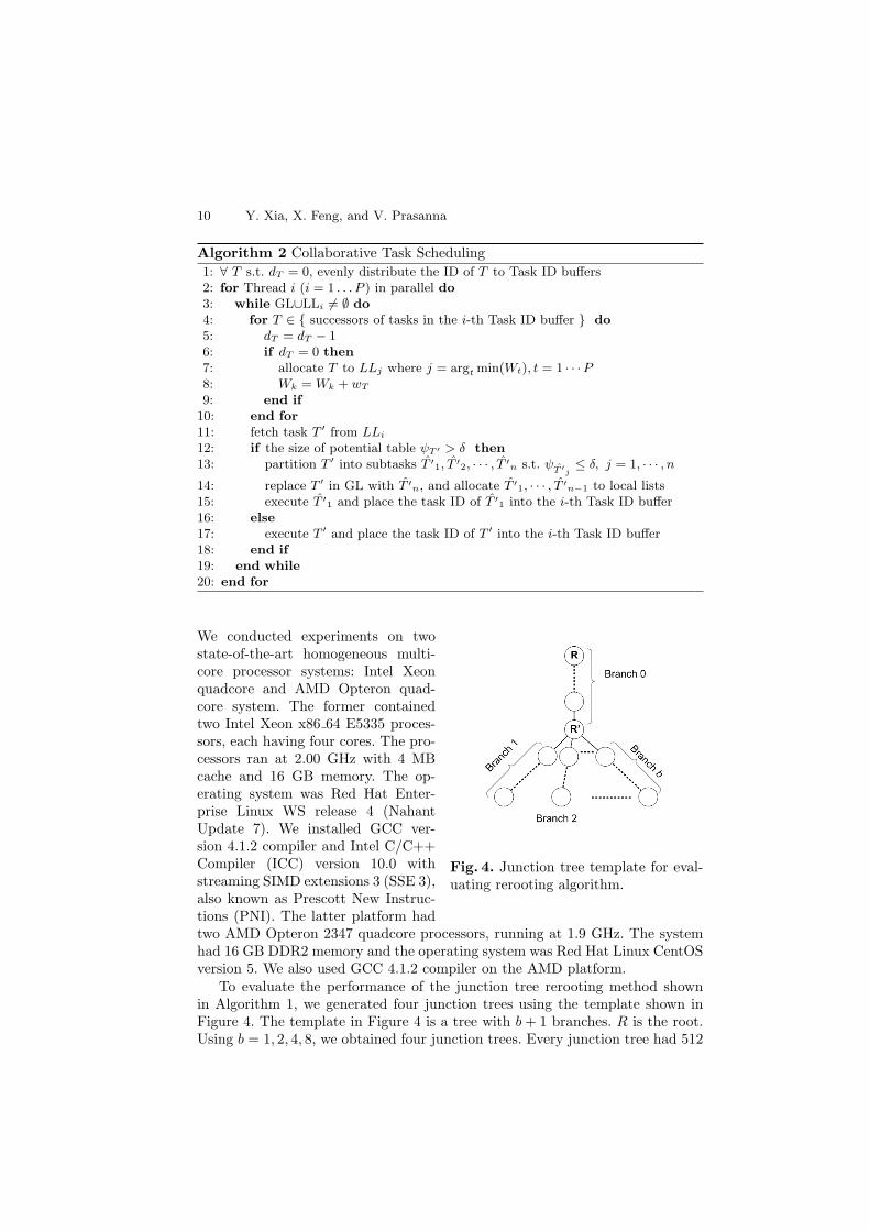
Fig. 4. Junction tree template for eval-uating rerooting algorithm.

We conducted experiments on twostate-of-the-art homogeneous multi-core processor systems: Intel Xeonquadcore and AMD Opteron quad-core system. The former containedtwo Intel Xeon x86 64 E5335 proces-sors, each having four cores. The pro-cessors ran at 2.00 GHz with 4 MBcache and 16 GB memory. The op-erating system was Red Hat Enter-prise Linux WS release 4 (NahantUpdate 7). We installed GCC ver-sion 4.1.2 compiler and Intel C/C++Compiler (ICC) version 10.0 withstreaming SIMD extensions 3 (SSE 3),also known as Prescott New Instruc-tions (PNI). The latter platform hadtwo AMD Opteron 2347 quadcore processors, running at 1.9 GHz. The systemhad 16 GB DDR2 memory and the operating system was Red Hat Linux CentOSversion 5. We also used GCC 4.1.2 compiler on the AMD platform.

To evaluate the performance of the junction tree rerooting method shownin Algorithm 1, we generated four junction trees using the template shown inFigure 4. The template in Figure 4 is a tree with b+ 1 branches. R is the root.Using b = 1, 2, 4, 8, we obtained four junction trees. Every junction tree had 512


cliques, each consisting of 15 binary variables. Thus, the serial complexity of eachBranch is approximately equal. Using Algorithm 1, clique R′ became the newroot after rerooting. For each junction tree, we performed evidence propagationon both the original tree and the rerooted tree, using various number of cores.We disabled task partitioning, which provided parallelism at fine grained level.

Fig. 5. Speedup caused by rerooting on (a) Intel Xeon and (b) AMD Opteron. (b+ 1)is the total number of branches in the junction tree.

The results are shown in Figure 5. The speedup in Figure 5 was defined asSp = tR/tR′ , where tR (tR′) is the execution time of evidence propagation inthe original (rerooted) junction tree. According to Section 4, we know that whenclique R is the root, Branch 0 plus Branch 1 is a critical path. When R′ is theroot, only Branch 0 is the critical path. Thus, the maximum speedup is 2 for thefour junction trees, if the number of concurrent threads P is larger than b. WhenP < b, Sp was less than 2, since some cliques without precedence constraint cannot be processed in parallel. From the results in Figure 5, we can see that thererooted tree led to speedup around 1.9, when 8 cores were used. In addition,the maximum speedup was achieved using more threads as b increases. Theseobservations matched the analysis above. Notice that some speedup curves fellslightly when 8 concurrent threads were used. This was caused by the overheadssuch as the lock contention.

We also observed that, compared with the time for evidence propagation,the percentage of overall execution time spent on junction tree rerooting wasvery small. Rerooting the junction tree with 512 cliques took 24 microsecondson the AMD Opteron quadcore system, compared to 2.8× 107 microseconds forthe overall execution time. Thus, although Algorithm 1 was not parallelized, itcauses negligible overhead in parallel evidence propagation.

We generated junction trees of various sizes to analyze and evaluate theperformance of the proposed evidence propagation method. The junction treeswere generated using Bayes Net Toolbox [12]. The first junction tree (Junctiontree 1) had 512 cliques and the average clique width was 20. The average degreefor each clique was 4. All random variables were binary. The second junction


tree (Junction tree 2) had 256 cliques and the average clique width was 15. Thenumber of states of random variables was 3 and the average clique degree was4. The third junction tree (Junction tree 3) had 128 cliques. The clique widthwas 10 and the number of states of random variables was 3. The average cliquedegree was 2. All the three junction trees were rerooted using Algorithm 1. Inour experiments, we used double precision floating point numbers to representthe probabilities and potentials.

Fig. 6. Scalability of exact inference using PNLlibrary for various junction trees.

We performed exact infer-ence with respect to the abovethree junction trees using In-tel Open Source ProbabilisticNetwork Library (PNL) [13].The scalability of the resultsis shown in Figure 6. PNLis a full function, free, opensource, graphical model li-brary released under BerkeleySoftware Distribution (BSD)style license. PNL providesan implementation for junc-tion tree inference with dis-crete parameters. The paral-lel version of PNL is also pro-vided by Intel [13]. The re-sults shown in Figure 6 wereobtained on a IBM P655 mul-tiprocessor system, where each processor runs at 1.5 GHz with 2 GB of memory.We can see from Figure 6 that, for all the three junction trees, the executiontime increased when the number of processors was greater than 4.

Fig. 7. Scalability of exact inference using various methods on (a) Intel Xeon and (b)AMD Opteron.


We compared three parallel methods for evidence propagation on both IntelXeon and AMD Opteron in Figure 7. The first two methods were the baselines.The first parallel method was the OpenMP based method, where the OpenMPintrinsic functions were used to parallelize the sequential code. We used ICCto compile the code on Xeon, while GCC was used on Opteron. The secondmethod is called data parallel method, where we created multiple threads foreach node level primitive. That is, the node level primitives were parallelizedevery time they were performed. The data parallel method is similar to thetask partitioning mechanism in our collaborative scheduler, but the overheadswere large. The third parallel method was the proposed method. Using Junctiontrees 1-3 introduced above, we conducted experiments on both the platforms.For all the three methods, we used level 3 optimization (-O3). The OpenMPbased method also benefited from the SSE3 optimization (-msse3). We showthe speedups in Figure 7. The results show that the proposed method exhibitedlinear speedup and was superior compared with the baseline methods on boththe platforms. Performing the proposed method on 8 cores, we observed speedupof 7.4 on Intel Xeon and 7.1 on AMD Opteron. Compared to the OpenMP basedmethod, our approach achieved speedup of 2.1 when 8 cores were used. Comparedto the data parallel method, we achieved speedup of 1.8 on AMD Opteron.

To show the load balance we achieved and the overhead of the collaborativescheduler, we measured the computation time for each thread. In our context,the computation time for a thread is the total time taken by the thread toperform node level primitives. Thus, the time taken to fetch tasks, allocate tasksand maintain the local ready list were not considered. The computation timereflects the workload for each thread. We show the results in Figure 8 (a), whichwere obtained on Opteron using Junction tree 1 defined above. We observedvery similar results for Junction tree 2 and 3. Due to space constraints, we showresults on Junction tree 1 only. We also calculated the ratio of the computationtime over the total parallel execution time. This ratio illustrates the quality ofthe scheduler. From Figure 8 (b), we can see that, although the scheduling timeincreased a little as the number of threads increases, it was not exceeding 0.9%of the execution time for all the threads.

Finally, we modified parameters of Junction tree 1 to obtain a dozen junctiontrees. We applied the proposed method on these junction trees to observe theperformance of our method in various situations. We varied the number of cliquesN , clique width wC , number of states r and average number of children k. Weobtained almost linear speedup for all cases. From the results in Figure 9 (a), weobserve that the speedups achieved in the experiments with various values for Nwere all above 7. All of them exhibited linear speedups. In Figure 9 (b) and (c),all results showed linear speedup except the ones with wC = 10 and r = 2. Thereason was that the size of the potential table was small. For wC = 10 and r = 2,the potential table had 1024 entries, about 1/1000 of the number of entries in apotential table with wC = 20. However, since N and the junction tree structurewere the same, the scheduling requires approximately the same time for junctiontree with small potential tables. Thus, the overheads became relatively large. In


Fig. 8. (a) Load balance across the threads; (b) Computation time ratio for each thread.

Figure 9 (d), all the results had similar performance when k was varied. All ofthem achieved speedups of more than 7 using 8 cores.

8 Conclusions

We presented an efficient rerooting algorithm and a collaborative schedulingalgorithm for parallel evidence propagation. The proposed method exploitedboth task and data parallelism in evidence propagation. Thus, even though one ofthe levels can not provide enough parallelism, the proposed method still achievesspeedup on parallel platforms. Our implementation achieved 7.4× speedup using8 cores. This speedup is much higher compared with the baseline methods, suchas the OpenMP based implementation. In the future, we plan to investigate theoverheads in the collaborative scheduler and further improve its performance.As more cores are integrated into a single chip, some overheads such as lockcontention will increase dramatically. We intend to improve the design of thecollaborative scheduler to reduce such overheads, so that the scheduler can beused for a class of DAG structured computations in the many-core era.

References

1. Lauritzen, S.L., Spiegelhalter, D.J.: Local computation with probabilities andgraphical structures and their application to expert systems. J. Royal StatisticalSociety B 50 157–224 (1988)

2. Heckerman, D.: Bayesian networks for data mining. In: In Data Mining andKnowledge Discovery. (1997)

3. Russell, S.J., Norvig, P.: Artificial Intelligence: A Modern Approach (2nd Edition).Prentice Hall (2002)

4. Segal, E., Taskar, B., Gasch, A., Friedman, N., Koller, D.: Rich probabilistic modelsfor gene expression. In: 9th International Conference on Intelligent Systems forMolecular Biology. 243–252 (2001)

5. Pennock, D.: Logarithmic time parallel Bayesian inference. In: Proceedings of the14th Annual Conference on Uncertainty in Artificial Intelligence. 431–438 (1998)


Fig. 9. Speedups of exact inference on multicore systems with respect to various junc-tion tree parameters.

6. De Vuyst, M., Kumar, R., Tullsen, D.: Exploiting unbalanced thread schedulingfor energy and performance on a cmp of smt processors. In: IEEE InternationalSymposium on Parallel and Distributed Processing (IPDPS). 1–6 (2006)

7. Kozlov, A.V., Singh, J.P.: A parallel Lauritzen-Spiegelhalter algorithm for proba-bilistic inference. In: Supercomputing. 320–329 (1994)

8. Xia, Y., Prasanna, V.K.: Parallel exact inference. In: Proceedings of the ParallelComputing. 185–192 (2007)

9. Xia, Y., Prasanna, V.K.: Node level primitives for parallel exact inference. In:Proceedings of the 19th International Symposium on Computer Architecture andHigh Performance Computing. 221–228 (2007)

10. Xia, Y., Prasanna, V.K.: Junction tree decomposition for parallel exact infer-ence. In: IEEE International Symposium on Parallel and Distributed Processing(IPDPS). 1–12 (2008)

11. Xia, Y., Prasanna, V.K.: Parallel exact inference on the cell broadband engineprocessor. In: Proceedings of the International Conference for High PerformanceComputing, Networking, Storage and Analysis (SC). 1–12 (2008)

12. Murphy, K.: (http://www.cs.ubc.ca/∼murphyk/software/bnt/ bnt.html)13. Intel Open Source Probabilistic Networks Library: (http:// www.intel.com/tech

nology/computing/pnl/)

Documents

Parallel Evidence Propagation on Multicore Processorshalcyon.usc.edu/~pk/prasannawebsite/papers/xia09pact.pdf · Parallel Evidence Propagation on Multicore ... applications in a number