PARALLEL DYNAMIC GRID REFINEMENT FOR INDUSTRIAL …

European Conference on Computational Fluid DynamicsECCOMAS CFD 2006

P. Wesseling, E. Onate and J. Periaux (Eds)c© TU Delft, The Netherlands, 2006

PARALLEL DYNAMIC GRID REFINEMENT FOR INDUSTRIALAPPLICATIONS

Thomas Alrutz∗, Matthias Orlt∗

∗ DLR German Aerospace CenterInstitute of Aerodynamics and Flow TechnologyNumerical Methods, 37073 Gottingen, Germany

e-mail: [email protected]: [email protected]

Key words: Grid adaptation, parallel dynamic refinement, unstructured hybrid grids, dis-tributed grid data-structures

Abstract. This paper covers a description of the algorithms and data-structures used in theparallel DLR TAU-Code Adaptation tool. Attention is given to the basic algorithms of theparallel anisotropic refinement and de-refinement, as well as the data-structures for distributedgrids and grid hierarchy. The parallelization issues for distributed data are discussed alongwith the dynamic repartitioning and the load-balancing algorithm.

To demonstrate the dynamic character of the TAU-Code adaptation, we choose a simulationfor a complex aircraft configuration and perform a parallel CFD calculation using varyingnumbers of CPUs. The obtained results show good parallel scalability with respect to memoryand CPU-time consumption.

1 INTRODUCTION

Local grid refinement for unstructured hybrid meshes is a common approach to improve theaccuracy of a solution for a given CFD problem or to reduce the amount of the points neededfor a numerical calculation4,12. Typically, this method starts with an initial grid for a partic-ular geometry. Subsequently, the grid is repeatedly locally adapted by inserting or removingpoints based on a local error estimation or an equidistribution of differences of appropriate val-ues derived from the current solution. The solution of larger CFD problems in an industrialenvironment requires the use of parallel software on distributed memory machines9. A goodload balance between the various processors is needed to achieve a high efficiency in a parallelCFD simulation. Each local refinement of the grid requires the grid partitions to be checked.Therefore, a dynamic grid partitioner with an efficient load-balancing algorithm8 has to be used.Moreover distributed grid data-structures and a distributed grid hierarchy are needed. In this pa-per, we present the data-structures and algorithms used in the TAU-Code adaptation and gridpartitioner and demonstrate their capability in a parallel CFD simulation for a fairly complexexample.

Thomas Alrutz, Matthias Orlt

2 The DLR TAU-Code

The DLR TAU-Code is a finite-volume Euler/ Navier-Stokes solver working on unstructuredhybrid grids. The code is composed of independent modules: Grid partitioner, a preprocessingmodule, the flow-solver and a grid adaptation module. The grid partitioner and the preprocess-ing are decoupled from the solver in order to allow grid partitioning and calculation of metricson a platform other than that used by the solver.

The parallelization of the flow solver is based on a domain decomposition of the computa-tional grid. Due to the explicit time stepping scheme, each domain can be treated as a completegrid. During a flux integration, data has to be exchanged between different domains severaltimes. In order to enable the correct communication, there is one layer of ghost points locatedat each interface between two neighbouring domains (see figure 1). The solid drawn vertices areinner points of the left domain as they are located on the left side of the cut. Each vertex of theright domain, which is connected to one of the inner points of the left domain, is a ghost pointof the left domain. All cut edges are part of both domains and are used for the communicationbetween those domains. An exchange of updated point data is necessary whenever an operationon the edges is performed. The exchange of the point data is done by employing the MessagePassing Interface (MPI).

Figure 1: Domain decomposition Figure 2: Ghost point creation

Further details of the TAU-Code solver and preprocessing may be found in13. In the nextsections we give a detailed overview of the algorithms and data-structures used in the gridpartitioner and adaptation module.

3 GRID PARTITIONING

First the computational grid is split into the number of desired domains for a parallel run ofthe TAU-Code. The grid partitioner uses a recursive bisection algorithm to compute the desirednumber of domains. This step includes the computation of the number of inner points for each

2


domain as well as the migration of all attached elements of these points to form a complete grid.The formation of the domain-to-domain overlap region is achieved by adding the ghost pointsto each of the domains (see figure 2). The result is a one cell overlap, which is sufficient forthe flow solver communication. The first partitioning of the grid can be done in sequential orparallel mode.

3.1 Distributed grid data-structure

The initial grid data-structure consists of a list of vertices and surface/volume elements alongwith some required information for the flow solver like boundary markers. The grid data-structure supports a various set of 3D and 2D polyhedra (table 1).

Elements E`

Volume SurfacePolyhedra Tetrahedra Prism Pyramid Hexahedra Triangle Quadrilateral# vertices 4 5 6 8 3 4

Table 1: Element overview

Let Ω ⊂ R3 be the complete domain and Γ ⊂ Ω the boundary. The TAU-grid T that coversΩ is therefore uniquely defined as a collection of the following sets :

1. A set of vertices V = xi ∈ Ω, 0 ≤ i < NV, a member of which is defined by itscoordinates.

2. One or more sets of volume and surface elements E` = Ti, 0 ≤ i < NE``=0,1,...,5, where

each type of element Ti is defined by the indices of the corner vertices.

3. A set of boundary markers for the surface elements M = Mi, 0 ≤ i < NE4 + NE5 , amember of which is defined by an associated boundary treatment.

However, the distributed grid data-structure requires some additional information. In order tocalculate the communication partners for the solver during the preprocessing and allow the gridpartitioner to work on the distributed grid domains, it is necessary to have the following sets aswell for each partition of the complete grid:

4. A set of ghost points V(k) = xi ∈ Ω, NV(k) ≤ i < NV(k) + NV(k), a member of which isconnected with at least one of the inner points of the partition k, with an edge.

5. A set of global point indices I(k) ⊂ I = 0, 1, . . . , NV − 1, where each entry is areference to the unique global index of a vertex in the initial grid.

6. A set of partition owners O(k) = di, 0 ≤ i < NV(k) |0 ≤ di < NProc, di 6= k of theghost points to relocate the partition where the original vertex is stored.

3


7. A set of the remote local indices R(k) = ri|0 ≤ ri < Vdi, 0 ≤ i < NV(k) of the ghost

points. This set holds the indices of the original vertex on the remote partition.

A partition of a grid is then defined as a collection of the sets

T (k) :=V(k), I(k), E (k)

` ,M(k),O(k),R(k)

, (1)

with V(k) = V(k) ∪ V(k).Considering we have Nproc partitions then it holds for every two partition p and q

V(p)

Nproc−1⋂p=0,q=0

V(q) = ∅, ; p 6= q =⇒ V =

Nproc−1⋃k=0

V(k). (2)

The sets O(k) and R(k) are used to calculate the communication interfaces for the MPI-transfer.

3.2 Super cell generation

For hybrid grids with quasi structured sub-layers containing prism or hexaehdral stacks, wehave implemented an algorithm to join each prism or hexahedra stack into a single surfaceelement for the calculation of the domain decomposition. We call those elements ”super cells”.The collapsing of a complete element stack into a super cell (figure 3), has two side effects.First is the reduced graph for the load balancing calculation. Secondly this feature preventssplit stacks due to the fact that the load balancing algorithm has no information about collapsedelements and is therefore only able to split a heavy weighted element. This specific feature isused in the y+ grid adaptation5.

Figure 3: Super cell generation

Timings for 30/1 iterations (4w) in secondsStandard Super cell

#CPU 30 1 30 11 811.6s 27.05s 811.6s 27.05s2 419.3s 13.98s 425.1s 14.17s4 207.1s 6.90s 209.2s 6.97s8 107.8s 3.59s 113.0s 3.77s

16 59.0s 1.97s 58.3s 1.94s24 43.0s 1.43s 42.7s 1.42s32 33.4s 1.11s 33.6s 1.12s

Figure 4: Parallel performance DLR-F63

4


3.3 Partitioning and load-balancing

The implemented recursive bisection algorithm is a effective way to achieve domain decom-position on a given grid7. The main idea is to split the grid along the medial x,y,z-axis andtry to find a decomposition of the domain with equally balanced partitions. Let G(V , E) be thegraph calculated from a given grid T and D be the set which indicates the current partition ofeach vertex. First, all vertices are sorted according to their coordinates in each dimension. Thealgorithm considers a cutplane for each dimension which is perpendicular to the coordinate axisand located at the coordinate value calculated by the median of

NV−1∑i=0

ω(σd(xi)), (3)

with ω being the point-weight function, σd the permutation of the vertices xi after the sort indimension d. By construction, each of the cut-planes will bisect the grid. The algorithm thenselects the cut-plane that cuts the smallest number of egdes. The subgrids are then consideredrecursively using the same technique. At the end of the algorithm for each vertex xi ∈ V exactlyone partition di, 0 ≤ di < NProc is stored in D.

For the use together with the super cells some changes are necessary. In order to have asimilar load balancing (compared to the case without the super cells) it is necessary to correctthe edge- and point-weights in the super cells. This is done by a summation of all edge- andpoint-weights in the elements corresponding to the super cell (see figure 3). Then a reduction ofthe set of vertices and edges is performed, such that the recursive bisection algorithm receivesonly the reduced Graph G(V , E).

We have performed several numerical experiments to investigate the influence of this ap-proach to the overall runtime of the flow solver and it was found, that there is no performancepenalty greater than the meausurement error (see figure 4). Further examination of the calcu-lation of the load-balancing leads to the assumption that, in the case of a hybrid grid, there arealways enough unstructured elements which can be used to compensate inbalance introducedby super cell generation.

The parallelization of the recursive bisection algorithm is straight forward for distributedgrids.

3.4 Parallel migration of unadapted grids

After the decomposition of the vertices on each process is done, we determine for eachvolume element Ti ∈ E` the processor / partition it will be migrated to. Each element will bemigrated to those partitions where its vertices are migrated to.

Let P = 0, . . . , NProc − 1 denote the available processors and D(k) = di, 0 ≤ i <NeV(k) |0 ≤ di < NProc be the set of the new partition owners of the vertices in T (k). We definethe map νk : V(k) 7→ P given by D(k). An element T

(k)i ∈ E (k)

` will then be moved to processorp if and only if one of its vertices will be moved to p:

T(k)i ∈ E (p)

` , ` = 0, 1, 2, 3 ⇐⇒ ∃ id ∈ T(k)i | νk(id) = p. (4)

5


For consistency reasons it is necessary to migrate the surface elements E (k)4 , E (k)

5 , and the bound-ary markers M(k) along with the volume elements. Thus if a volume element and a surfaceelement share a common face

T (k) ⊂ T

(k)i , T (k)

∈ E (k)ı , ı = 4, 5, T

(k)i ∈ E (k)

` , ` = 0, 1, 2, 3 (5)

the surface element has also to be moved to the partition where the volume element goes.Before the volume and surface elements can be sent to their new partitions, all their local

indices have to be transfered into the global index space, which are the original indices of theassociated vertices. This is done by rewriting an index id ∈ T

(k)i ∈ E (k)

` with the correspondingvalue from I(k). The mapping of the local indices into the global index space gurantees thecorrect reordering of the point indices at the receiving partition.

At the end of the migration process, the vertices are migrated corresponding to their newowners given by D(k). This is done in several steps, because of the differentiation betweeninner and ghost points. The inner points can be sent directly to their new owners togetherwith their global indices from I(k). The ghost points on the other hand must be calculated foreach partition seprately. A ghost point is always created in the case when not all vertices ofan element are moved to the same partition. Consider an element T

(k)i which is sent to the

partitions p and q. For each vertex xid, id ∈ T(k)i , which is not sent to q a ghost point has to be

created on the partition q. Thus

∀ id ∈ T(k)i with νk(id) 6= q (6)

we create a ghost point entry with vertex xid for the partition q. This is done for all partitionsto where the element T

(k)i is migrated. Then the collection of ghost points can be sent to these

partitions together with the corresponding global indices and partition owners. On the receiverside it is quite easy to collect all elements and store them in the corresponding sets. For thevertices some additional work is required. First receive all the inner points and sort them inincreasing order corresponding to their global indices. Then receive all ghost points and killdouble entries. At the end remap all global point indices in the elements back to local partitionindexing. This can be done for each element with the effort of O(log(NeV(p))) by simply sortingthe set of global indices I(k) and emploing a binary search on the sorted set for each globalindex. The migration finish with the restablishment of the set R(p) by sending all the globalindices of the ghost points to their owner partitions for a calculation of the local remote indices.This data is then sent back to the initiating partition / process and the migration of the grid iscomplete.

4 GRID ADAPTATION

The adaptation module of the TAU-Code consists of three different components for variousgrid manipulations to adapt a given grid to the solved flow field:

• y+ based grid adaptation to adjust the first wall distance over turbulent surfaces in hybridgrids,

6


• hierarchical grid refinement and derefinement to introduce new grid points on a givenegde-indicator function without producing hanging nodes,

• surface approximation and reconstruction for curved surfaces after introduction of newgrid points.

In this paper our main focus is on the grid refinement and derefinement algorithms along withthe parallelization issues. An overview of the y+ based grid adaptation can be found in5.

4.1 Grid refinement

The basic concept of the local grid refinement and derefinement is similar to the red/greenrefinement6,10. After briefly summarising the TAU specific features of the basic algorithm4, theattention is turned to the concepts and algorithms of derefinement and parallel adaptation.

4.2 Basic algorithm of the local refinement

The main requirements of a local refinement strategy are the detection of grid areas whichare to be refined and the method of element subdivisions, which result from insertion of newpoints to these areas. A very rough draft of the basic algorithm reads as follows:

1 Build edge list and element to edge reference.

2 Evaluate edge indicators Ie.

3 Refine edge list considering the edge indicators,the target point number and the grid conformity.

4 Calculate coordinates of new points.

5 Construct new elements.

6 Interpolate solution to new points.

TAU-adaptation uses an edge based approach, i.e. The refinement indicators are evaluated forall edges, new points are inserted to the edge mid points and the element subdivisions aredetermined from the configuration of refined edges. Therefore, it builds the edge list and theelement to edge reference as the first step.

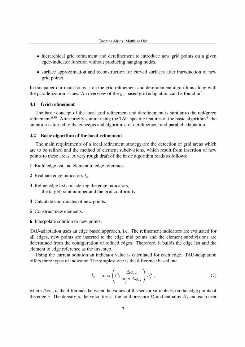
Using the current solution an indicator value is calculated for each edge. TAU-adaptationoffers three types of indicator. The simplest one is the difference based one

Ie = maxi

(Ci

∆φi,e

maxe

∆φi,e

)hα

e , (7)

where ∆φe,i is the difference between the values of the sensor variable φi on the edge points ofthe edge e. The density ρ, the velocities v, the total pressure Pt and enthalpy Ht and each user

7


defined variable written out by TAU-solver are available as sensors. The Maximum maxe ∆φi,e

over all edges is used as a normalisation constant if the sensors are of different order of magni-tude. This allows the user to weight the different sensors by Ci. Additionally, the differencesare scaled with the α power of the edge length he. The choice of the parameter α controlsthe stronger refinement of areas with smaller or larger cell sizes or inhibits the refinement ofdiscontinuities..

The other availaible indicator types are a gradient based indicator using the differences of thegradients of the sensor variables instead of the values itself. Finally, the reconstruction basedindicator considers the differences of the second order representation of the flow variable withinboth the edge points dual cells on the edge mid point, i.e. at the border face of the dual cells ofused vertex centered Finite Volume Method. However, each combination of indicator type andsensor indicates areas with a lack of a accurate representation of the current solution in somesense.

Step 3 of the simplified program flow consists of two nested loops. The outer refinementloop finds the Limit L for the indicator which results in the target number of new points if alledges with Ie > L are initially marked for refinement. In the inner consistency loop goes overall elements inserts additional points to get a valid subdivision case for each element and has tobe repeated until no points have to be added because changes can run through the grid.

The set of implemented refinement cases of the element types mainly determines how manyedges have to be marked unintended. A special feature of TAU-adaptation is the implementedcomplete set of tetrahedra subdivisions (see Figure 5). A continued marking of edges not ini-tially marked occurs to preserve the semistructured areas of Navier-Stokes-grids but stops if atetrahedral area is found. The admissible prism refinement cases (Figure 6) have an identicalrefinement of base and top triangle to obtain only new prisms. Pyramids are considered to be anunintended exception where the height of prism layers varies. So, there is only one refinementcase for pyramids (Figure 7) and the continued edge marking in pyramids has to be stopped inthe tetrahedral neighbourhood.

After determination of the final edge subdivision all marked edges are identified with newpoint numbers and the coordinates of these new points are calculated using a spline interpolationfor new surface points to consider curved surfaces (step 4 of basic algorithm). The new elementsare constructed using the appropriate subdivisions (Figure 5, 6, 7) in step 5. Finally, the solutionis interpolated to the new points (step 6).

In the strict sense, this representation of TAU-adaptation is correct only for the first adapta-tion step. All element subdivision cases except the trival refinement cases (a) for tetrahedra andprisms and the isotropic refinement for tetrahedra with an additional condition for the choiceof the inner diagonal (l) and semi-isotropic refinement for prisms (c), potentially lead to morestreched elements and to a lower grid quality. Therefore TAU-adaptation uses a red/green liketechnique even in the refine-only-mode to avoid degeneracy of elements. Because its algorithmuses the grid refinement hierarchy, the description is postponed until the next subsection aboutderefinement of TAU-adaptation.

8


!!!!!

QQ

Q

%%

%%

%%

AA

AA

AA

no edge marked1 tetrahedron (a)

!!!!!

QQ

Q

%%

%%

%%

AA

AA

AA

1 edge marked2 tetrahedra (b)

!!!!!

QQ

Q

%%

%%

%%

AA

AA

AA

##

##

#

SS

SS

2 (opp.) edges marked4 tetrahedra (c)

!!!!!

QQ

Q

%%

%%

%%

AA

AA

AA

QQ

2 edges marked3 tetrahedra (d)

!!!!!

QQ

Q

%%

%%

%%

AA

AA

AA

QQ !!!

BB

BBB

3 edges (on 1 face) marked4 tetrahedra (e)

!!!!!

QQ

Q

%%

%%

%%

AA

AA

AA

QQ%

%%

SS

SS

3 edges marked5 tetrahedra (f)

!!!!!

QQ

Q

%%

%%

%%

AA

AA

AA

QQAA

A

3 edges (at 1 node) marked4 tetrahedra (g)

!!!!!

QQ

Q

%%

%%

%%

AA

AA

AA

QQ %

%%

QQ

%%

%

4 (opp.) edges marked6 tetrahedra (h)

!!!!!

QQ

Q

%%

%%

%%

AA

AA

AA

QQ !!!%

%%

AA

A

BB

BBB

4 edges marked6 tetrahedra (i)

!!!!!

QQ

Q

%%

%%

%%

AA

AA

AA

QQ !!!%

%%!!!

AA

AA

AA

BB

BBB

5 edges marked7 tetrahedra (k)

!!!!!

QQ

Q

%%

%%

%%

AA

AA

AA

QQAA

A

!!!%%

%

%%

%!!!

AA

AQQ

6 edges marked8 tetrahedra (l)

Figure 5: Tetrahedra refinement cases

4.3 Refinement hierarchy for derefinement and no-degeneracy

The application of local grid refinement strategy to an unsteady simulation requires the pos-sibility to remove previously inserted grid refinements if the flow phenomenon causing thisrefinement has departed from the grid region. Also in a steady calculation it can be helpful touse derefinement if flow phenomena are resolved only after several adaptation steps and changethe character of the flow to some extent. In this case the combined re- and derefinement is ableto remove points inserted by early adaptation steps based on not fully converged solutions andnot needed for the converged solution.

Because TAU-adaptation does not perform a proper grid coarsening it has to store the refine-ment hierarchy in order to restore the original elements later. The refinement hierarchy containslists of parent elements of each element type and stores the actual hierarchical reference forthese parent element lists. This is done in a bottom to top manner, i.e. each element and eachparent have references to their direct parent (parent reference), i.e. the element (not existing inthe current grid) whose subdivision generated it. Figure 8 illustrates the situation. Some ele-ments may and some parents must have the information that they are initial elements instead ofthe parent reference. Additionally all elements and parents having a parent have the informationwhich element of the element subdivision they are (child type). Also the information about the

9


@@@

@@@

no edge marked1 prism (a)

@@@

@@@

1 base edge marked2 prisms (b)

@@@

@@@

@@

@@

3 base edges marked4 prisms (c)

Figure 6: Prism refinement cases

DDDDDDD

SS

SS

S

no edge marked1 pyramid

DDDDDDD

SS

SS

S

ll

ll

ll

ll

HHHHH

HHHHH

DDDDDDD

SS

SS

S

SSS

DDDD

DDDD

SSS

ll

ll

ll

ll

HHHHH

HHHHH

DDDD

SSS

PP

2 base edges and 4 vertical edges marked2 pyramids and 7 tetrahedra

Figure 7: Pyramid refinement cases

applied subdivision case (refine type) is stored for all parents.Now TAU-adaptation works on the current elements and their direct parents switching from

one to another in case of refinement or derefinement, respectively. The preliminary step 1 of thebasic algorithm is extended to the algorithm sample shown in the following pseudo code.

1.1 Determine direct parents of the actual elements.

1.2 Build edge list of elements and direct parents.Build element to edge reference of elements and of direct parents.

1.3 Restore mid points of the parent edges.

1.4 Forbid all edges not in isotropic refinements for indication.

1.5 Forbid all edges having a parent point for derefinement.

Step 1.1 is easily done by flagging all parents which are referenced to by other parents andconsidering the remaining parents. While step 1.2 basically works as the former step 1 did steps1.3 – 1.5 use the refine type of the direct parents and the child typ of the actual elements and ofcourse the element/parent to edge references.

The refinement step also has to be modified for derefinement:

10


...

12no

1123

child typeof elements

...

PPPPPPPqhhhhhhh- no p.

--

(((((((

1

parentreference

of elements

...

- no p.- no p.y

parentreferenceof parents

...

1:21:21:3

refinetype ofparents

...

nono

2

childtype ofparents

Figure 8: Refinement hierarchy of TAU-adaptation.

3.1 Set an initial guess for the indicator limit L.

3.2 Mark all parent edges with Ie < L s for derefinement.

3.3 Mark all edges with Ie > L/s for refinement.

3.4 Mark additional edges for refinementif needed to get a valid refinement case (consistency loop).

3.5 Count marked edges (i.e. number of new points).If percentage of new points is to large or too smallcorrect L, reset re- and derefinements and goto 3.2.

The parameter s with 12

< s ≤ 1 of steps 3.2 and 3.3 is intended to produce some inertiafor the point movement in the grid and so to stabilise a multiple adaptation and improve theconvergence especially of a steady calculation. In an unsteady simulation one might want to sets = 1 especially if the local grid refinement has difficulties in following the flow phenomenawhich are to be resolved maybe if the time steps are fairly large or one do not adapt in each timestep.

To avoid element degeneracy elements resulting from non-isotropic subdivisions are not fur-ther refined. If such an element has to be refined because some of its edges are marked forrefinement, the direct parent element is isotropically refined and the remaining edge marksconsidered in the resulting children. This leads to the further refinement of some of the newelements which become parents themself and are written to the parent lists and considered inthe hierarchy data structure. This situation is illustrated in the top line of Figure 9. In the sameway, if the edge refinement of a direct parent has changed algorithm works on this parent. Thisparent can change its refinement type or be completely derefined. In the latter case it goes back

11


%%

%%

AA

AA

×−→

%%

%%

AA

AA

× −→

%%

%%

AA

AA

AA

%%

Further refinement of a trianglemarked edges for refinement by indicator (×)

by algorithm ()

%%

%%

AA

AA

AA

%%

×−→

%%

%%

AA

AA

AA

%%

×× × −→

%%

%%

AA

AA

Derefinement of a multiply refined triangleedges marked for derefinement (×)

edges forbidden for derefinement ()

Figure 9: Further refinement and derefinement.

to the elements list and is removed from the parent element list. On the other hand if the al-gorithm works on an element and the element has to be subdivided, the children are written tothe new grid, the former element is written to the parent lists and the corresponding hierarchyinformation is added.

Because TAU-adaptation considers only direct parents only the latest refinement level canbe removed (see bottom line of Figure 9). A multiple refinement and the following completederefinement would generate different intermediate grids as a consequence.

4.4 Parallel grid refinement

The TAU-Code uses the vertex orientated type of domain decomposition holding the addi-tional points of the overlapping elements with lists storing their owner domain and local pointnumber in their own domain (communication map). The main steps of TAU-adaptation workin an element orientated way and each of the parent elements of the grid hierarchy is storedonly in one of the domains. So the adaptation needs some simple rules to clearly determine theownership of elements and edges, and some communication to reinforce the TAU-Code formatof grid domains in the end.

Because the parallel adaptation must provide the same result as a serial adaptation, the indi-cator limit has to be the same on all domains. Therefore one cannot expect to have load balanceddomains after a parallel local grid adaptation without grid repartitioning. In examples with astrong local refinement, e.g. at discontinuities, it is difficult or impossible to get a load balancewithout distributing the children or grand children of an initial element over various domains ingeneral. So the grid hierarchy needs an extension allowing to refer to other domains.

In order to use the same algorithms as in the serial version and to minimise the numberof communications between domains, all elements having a parent are sent to the domain ofits direct parent. In general, this step enlarges the number of additional points, i.e. points of

12


other domains needed in this domain to define the overlap elements and the children of own(overlapping) direct parents. A simple rule of element ownership is the element belongs to andis considered by the domain of its direct parent. All initial elements having only own points ofthe domain are known only in this domain and are refined or derefined there. Initial elementsof the overlap area are identified by its additional points, i.e. they have domain own points andpoints belonging to other domains. These elements determine their owner domain with a simplerule, e.g. the owner of the smallest global point number.

These extensions lead to the following modification of the algorithm:

1.1 Send all elements to the domain of their direct parents.

1.2 Determine direct parents of the actual elements.

1.3 Build edge list of elements and direct parents.Build element to edge reference of elements and of direct parents.

1.4 Build communication tables for edges.

1.5 Restore mid points of the parent edges.

1.6 Forbid all edges not in isotropic refinements for indication.

1.7 Forbid all edges having a parent point for derefinement.

A lot of edge information has to be communicated between domains because the informationabout restored points on the parent edges, about the admissibility of an initial mark for refine-ment and about the refinement state is needed in all domains having the edge. So in favour ofefficiency it is worth to build edge tables holding the edge numbers corresponding to a positionin lists to send to and receive from other domains. Therefore step 1.4 prepares steps 1.5–1.7and especially the communication of the refinement state within the refinement loop (compareto steps 3.3 and 3.4 of pseudo code). Different from the communication of point related infor-mation in the TAU-solver, the adaptation has to communicate the edge information from eachdomain to each other domain containing the edge. In order to minimise the total amont of trans-fered information, an owner domain of the edge is defined by the following: the domain owningthe edge point with the smaller global point number is the owner of the edge. All edges sendtheir state information to the owner domain of the edge. After determining the resulting state,the edge information is sent back to all other domains having this edge.

After the re- or derefinement is done and the new elements are constructed some additionalsteps are needed to re-establish the point oriented domain decomposition.

5.1 Construct new elements.

5.2 Determine the owner domain of the new points.

5.3 Update point communication map.

13


5.4 Send elements to the owner partition.

5.5 Remove pure addpoint elements.

5.6 Permutate points.

Data structures of TAU-Code and algorithms of TAU-adaptation allow to arbitrarily assign thenew points to the domains, e.g. to the owner domain of the edge the new point originates from.The explicit determination of the new point owner in step 5.2 takes into consideration additionalrequirements of Y+-adaptation and partitioning.

In the next step 5.3 the communication map is updated, i.e. the lists holding the ownerdomain and the local point numbers of the additional points, for the new points using the edgecommunication tables again.

At this point of algorithm all the new elements and the parent elemenets reside only in oneof the domains. Thus after sending each element to every domain possessing at least one pointof the element (step 5.4) each domain has got all its own and overlapping elements. As in step1.1 this may enlarge the number of additional points. Because of the unique occurance of allelements before 5.4 there is no need to check or sort the received elements after 5.4. In theparent element lists still no parent occures twice and there is no need to change this.

Because of step 1.1 and because of a possible subdivision of a former overlapping elementa domain can have elements consisting of addpoints only. These elements are not needed andremoved in step 5.5. The derefinement and the last step can lead to disconnected points. There-fore step 5.6 re-esteblishes the order of own and additional points and removes the disconnectedones.

5 REPARTITIONING

As descripted in section 4 several information are required for an adapted grid. If we take acloser look at this structure, it can be seen that the parents are stored and handled the same wayas the children. However, the element hierarchy information is required to be stored.

5.1 Distributed grid hierarchy

Along with the sets from section 3.1 a hierarchy for a given grid T is given by the followingsets (e.g figure 8):

8. One or more sets of volume and surface parents E` = Ti, 0 ≤ i < NE``=0,1,...,5, where

each type of a parent Ti is defined by the indices of the corner vertices.

9. One or more sets of hierarchy references for the children H` = pidi, 0 ≤ i < NE`| −

1 ≤ pidi < NE``=0,1,...,5. Each entry refers to a parent in E` or is set to −1 in case of no

parent.

10. One or more sets of hierarchy references for the parents H` = pidi, 0 ≤ i < NE`| −1 ≤

pidi < NE``=0,1,...,5.Each entry refers to a parent in E` or is set to−1 in case of no parent.

14


11. One or more sets of child type classification for the children C` = cti, 0 ≤ i < NE``=0,1,...,5.

12. One or more sets of child type classification for the parents C` = cti, 0 ≤ i < NE``=0,1,...,5.

13. One or more sets of parent type classification for the children S` = pti, 0 ≤ i <NE`

`=0,1,...,5.

14. One or more sets of parent type classification for the parents S` = pti, 0 ≤ i <NE`

`=0,1,...,5.

15. One or more sets of refine type classification for the parents Z` = rti, 0 ≤ i <NE`

`=0,1,...,5. Each entry indicates the type of refinement of the associated parent.

In order to handle a distributed grid hierarchy additional information is needed:

16. A set of parent points V(k) = xi ∈ Ω, NV(k) + NV(k) ≤ i < NV(k) + NV(k) + NV(k).

17. A set of partition owners O(k) = di, 0 ≤ i < NV(k) |0 ≤ di < NProc, di 6= k of theparent points to relocate the partition where the original vertex is stored.

18. A set of remote local indices R(k) = ri|0 ≤ riVdi, 0 ≤ i < NV(k) of the parent points.

This set holds the indices of the original vertex on the remote partition.

19. One or more sets of partition owners of the parents L(k)` = di, 0 ≤ i < NE(k)

`|0 ≤ di <

NProc, di 6= k`=0,1,...,5 for the chidren.

20. One or more sets of partition owners of the parents L(k)` = di, 0 ≤ i < NE(k)

`|0 ≤ di <

NProc, di 6= k`=0,1,...,5 for the parents.

In the case of an adapted partitioned grid we write the set of vertices as a union of inner, ghostand parent points as in section 3.1 (V(k) = V(k) ∪ V(k) ∪ V(k)).

As the parents are only considered in the grid adaptation module, there is no need to storethem on more then one partition. This means a parent is stored uniquely at one location and thesets of different partitions are disjoint to each other. Furthermore there is no need to considerthe parents for the creation of a partition or for the load-balancing algorithm. This means forrepartitioning after grid adaptation the algorithm described in section 3 is used to calculate thepartitions.

5.2 Parallel migration of grid hierarchy

First for each of the parents the partition where the parent should be migrated to is deter-mined. Let P = 0, . . . , NProc − 1 be as in section 3.4 and D(k) = di, 0 ≤ i < NeV(k) |0 ≤di < NProc the set like in section 3.4 extended with the information about the parent points.Again we will define the map νk : V(k) 7→ P defined by D(k). Let n(`) denote the number ofcorner vertices of a parent element (table 1).

15


We determine the new partition p of a parent T(k)i ∈ E (k)

` , ` = 0, 1, 2, 3 by

T(k)i ∈ E (p)

` ⇐⇒ #tj | νk(tj) = p0≤j<n(`) ≥ #tj | νk(tj) = q0≤j<n(`), tj ∈ T(k)i , (8)

with 0 ≤ p < q < NProc. The surface parents (E (k)4 , E (k)

5 ) are migrated in the same way astheir children described in section 3.4. All the other information like the hierarchy reference ismigrated along with the elements and parents. The main problem is the correct reordering of theparent references H(k)

` and H(k)` . To do this properly in parallel the same approach as with the

indices of the vertices is employed. Thus before sending the parents and the hierarchy referenceinformation to the new partition owners, all the reference information in H(k)

` and H(k)` has to

be maped into the the global hierarchy index space I` = H` ∪ H`.The global hierarchy index of a parent is obtained by summing up the number of parents on

all partitions for each type. After the total number of each parent type is calculated, the uniqueglobal hierarchy index pid of a parent on partition k can be calculated with

pidi := i +k−1∑p=0

NE(p)`

,∀ T(k)i ∈ E (k)

` , ` = 0, 1, . . . , 5. (9)

The calculated values for all parents are stored in the set I(k)` in order to convert the local

hierarchy references into global hierarchy references. We define the map γ(k)` : H(k)

` 7→ H` andγ

(k)` : H(k)

` 7→ H` given by I(k)` . All elements and parents which satisfy

pidi ∈ H(k)` | di = k, di ∈ L(k)

pti , pti ∈ S(k)` , (10)

pidi ∈ H(k)` | di = k, di ∈ L(k)

pti , pti ∈ S(k)` (11)

can be handled direct with γ(k)` . In the case of a remote parent di 6= k, the information has to be

obtained by sending a querry to the partition where the remote parent is stored using the ownerinformation from L(k)

` or L(k)` . The global hierarchy index is then obatained as follows

pidi ∈ H(k)` | di = p, di ∈ L(k)

pti , pti ∈ S(k)` =⇒ pidi = γ

(p)` (pidi), (12)

pidi ∈ H(k)` | di = p, di ∈ L(k)

pti , pti ∈ S(k)` =⇒ pidi = γ

(p)` (pidi) (13)

and sent back together with the information about the new owner partition of this parent.After all the information is gathered together the hierarchy references H(k)

` , H(k)` can be

mapped into the global hierarchy index space on each partition without further communicationeffort. All the information about the hierarchy is then packed together with the elements andparents and is sent to the new owner partitions. On the receivers side p the data is collectedand the parents are sorted due to their unique global hierarchy index in I(p)

` in increasing order.The remapping to the local hierarchy index is done as described in section 3.4 for the indices ofthe elements. In order to get the local hierarchy index of all parents which are not on the local

16


partition, the same algorithm as in section 3.4 for the ghost points is used, to determine theremote indices. The convertion of the indices of the vertices in the sets of parents from local toglobal and back again is done by using the algorithm described in section 3.4 for the elements.The migration finishes with the restablishment of the set R(p), which is done by employing thealgorithm used for the calculation of R(p) in section 3.4.

6 APPLICATION EXAMPLES

In this section we apply the parallel adaptation and the parallel grid partitioner for two aero-dynamic configurations. The first is a generic delta wing presented in1 and the second is a A380configuration presented in11.

(a) Delta wing sketch (b) A380 configuration sketch from11

Figure 10: Sketch of delta wing (a) and A380 configuration (b)

6.1 Delta wing

The first example consists of adapting the mesh for a generic delta wing used to investigatethe vortex breakdown in a pitching manouver. The initial mesh has approximately 1× 106 gridpoints and around 2.5× 106 volume elements (figure 10 (a)).

(a) coarse (b) adapted (c) performance evaluation

Figure 11: Cut of the grids at x = 200 (a,b), performance on a Linux Opteron cluster with Gigabit (c)

17


It consists of an inner region of 1.9 × 106 prisms in 20 layers for the boundary layer andan outer region of 650000 thetrahedra. After several steps of adaptation we achieved a totalnumber of 4.47 × 106 grid points, around 15 × 106 volume elements and 4.17 × 106 parents.This grid was then used for a performance evaluation of the parallel adaptation method. It canbe seen in figure 11 (c) that the parallel adaptation and the partitioner scale quite well. Eventhe overall time from the initial sequential grid partitioning, the parallel adaptation and theparallel repartitioning is smaller then the time needed for the sequential adaptation. In this casea speedup of 4.4 for 8 CPUs and 5.4 for 16 CPUs could be achieved.

6.2 A380 configuration

The second example consists of adapting the mesh for a AIRBUS A380 in high-lift config-uration used to simulate the jet-flow behind the aircraft on ground (mach = 0) including theinteraction of the jet-flow with a hangar (see sketch in figure 10 (b)). The initial mesh has ap-proximatly 6.65 × 106 grid points and around 25 × 106 volume elements (figure 12 (a)). The

(a) initial grid (b) 3 times adapted (c) 6 times adapted

Figure 12: Surface mesh initial (a), 3 times adapted (b) and 6 times adapted (c)

mesh is 6 times adapted using the indicator in equation (7) with α = 1.00 and φi = |v| toachieve a total number of 12× 106 grid points and 55× 106 volume elements (figure 12 (c)).

Adaptation steps - timinings include repartitioning#CPU 1 2 3 4 5 6

1 -/- 484.37s -/- 635.85s -/- 769.37s16 54.53s 54.97s 55.16s 57.07s 55.08s 83.05s

#Points 7.5 ∗ 106 9.3 ∗ 106 10.2 ∗ 106 11.9 ∗ 106 11.5 ∗ 106 12 ∗ 106

Speedup -/- 8.81 -/- 11.52 -/- 9.26

Table 2: Comparison of the performance of the parallel and sequential adaptation with the A380 configuration(performed on a Linux Opteron cluster with Infiniband interconnect)

In figure 13 it can be seen, that the repartitioning algorithms performs quite well, as the pointsmove into the area of the jet-blast with each subsequent adaptation step. Here the repartitioning

18


ensures equally loaded partitions after refinement and de-refinement. Furthermore it can beseen that the adaptation removes points from the area of the hangar and distributes them intothe area around the jet-blast (figure 13 (b,c)).

Finally the timing statistics for the A380 configuration are listed in table 2 together with thedimension of the constructed grids. The overall speedup gain by using the parallel adaptationand partitioner, compared to the sequential adaptation is between 8.8 and 11.5.

(a) 1 time adapted (b) 2 times adapted

(c) 3 times adapted (d) 6 times adapted

Figure 13: Evolution of the adapted grids splitted in 16 partitions

7 Conclusions

The presented approach to handle distributed grids with grid hierarchy information in theTAU-adaptation shows a good overall scalability. Together with the dynamic repartitioningafter adaptation, the code can be used in a fully parallel simulation system enabling an engi-

19


neer or researcher to adapt several times without suffering from the bottleneck of a sequentialgrid adaptation or to change at any time within a calculation the number of partitions on thefly. Compared to a approach presented in8, where the parallel mesh adaptation has to keep abackground mesh on each processor in order to calculate a appropriate refinement sensor, theTAU-adaptation is capable to scale also with respect to memory consumption. This is due tothe fact, that the complete grid with its hierachy can be distributed over all the available CPUsfor a numerical simulation without storing a global array on any processor.

Despite the established features, there is still need for a further speedup of the refinementand de-refinement algorithm and for parallel initial grid partitioning.

References

1. T. Alrutz and M. Rutten. Investigation of Vortex Breakdown over a Pitching Delta Wingapplying the DLR TAU-Code with Full, Automatic grid adaptation. Paper 5162, AIAA,2005.

2. Thomas Alrutz. Erzeugung von unstrukturierten Netzen und deren Verfeinerung anhanddes Adaptationsmoduls des DLR-TAU-Codes. Diplomarbeit, Universitat Gottingen, 2002.

3. Thomas Alrutz. Investigation of the parallel performance of the unstructured DLR-TAU-Code on distributed computing systems. In Proceedings of Parallel CFD 2005 (accepted),2005. Egmond aan Zee, The Netherlands, May 21-23.

4. Thomas Alrutz. MEGAFLOW — Numerical Flow Simulation for Aircraft Design Results ofthe second phase of the German CFD initiative MEGAFLOW presented during its closingsymposium at DLR, Braunschweig, Germany, December 10th and 11th 2002, volume 89 ofNotes on Numerical Fluid Mechanics and Multidisciplinary Design, chapter 7 Hybrid GridAdaptation in TAU, pages 109–116. Springer Verlag, Berlin, 2005.

5. Thomas Alrutz and Tobias Knopp. Near wall grid adaption for wall functions. In Proceed-ings of International Conference on Boundary and Interior Layers 2006 (submitted), 2006.University of Gottingen, July 24-28.

6. J. Bey. Tetrahedral grid refinement. Computing, 55:355–378, 1995.

7. Feng Cao, John R. Gilbert, and Shang-Hua Teng. Partitioning meshes with lines and planes.Technical report, Xerox Palo Alto Research Center, January 1996.

8. Amik St-Cyr Claude Lepage and Wagdi Habashi. Parallel Ustructured Mesh Adaptationon Distributed-Memory Systems. paper 2004-2532, AIAA, 2004.

9. Norbert Kroll, Thomas Gerhold, Stefan Melber, Ralf Heinrich, Thorsten Schwarz, andBritta Schoning. Parallel Large Scale Computations for Aerodynamic Aircraft Design withthe German CFD System MEGAFLOW. In Proceedings of Parallel CFD 2001, 2001.Egmond aan Zee, The Netherlands, May 21-23.

20


10. D.J. Mavriplis. Adaptive Meshing Techniques for Viscous Flow Calculation on Mixed-Element Unstructured Meshes. paper 97-0857, AIAA, 1997.

11. S. Melber-Wilkending. Aerodynamic Analysis of Jet-Blast using CFD considering as ex-ample a Hangar and an AIRBUS A380 configuration. Technical report, STAB, 2004.

12. Jens-Dominik Muller. Anisotropic adaptation and multigrid for hybrid grids. NumericalMethods in Fluids, 40(3-4):445 – 455, 2002.

13. Dieter Schwamborn, Thomas Gerhold, and Roland Kessler. The DLR-TAU Code - anOverview. In Proceedings ODAS 99, 1999. ONERA-DLR Aerospace Symposium 21-24June in Paris, France.

21

Documents

PARALLEL DYNAMIC GRID REFINEMENT FOR INDUSTRIAL …