Embed Size (px)
Citation preview
Parallel Distributed Systems
Parallel &
Distributed
Systems
B.E. COMPUTER ENGINEERING (CPC803)
2015-2016
ANURADHA BHATIA
CBGS
M.E. Computer Engineering
MU
Parallel & Distributed Systems
Anuradha Bhatia
Table of Contents
1. Introduction .................................................................................................................................................... 1
2. Pipeline Processing ................................................................................................................................... 36
3. Synchronous Parallel Processing ......................................................................................................... 52
4. Introduction to Distributed Systems .................................................................................................. 65
5. Communication .......................................................................................................................................... 88
6. Resource and Process Management.................................................................................................. 124
7. Synchronization ....................................................................................................................................... 153
8. Consistency and Replication ................................................................................................................ 177
Parallel & Distributed Systems
Anuradha Bhatia
Disclaimer
The content of the book is the copyright property of the author, to be used by the students for
the reference for the subject “Parallel and Distributed Systems”, CPC803, Eighth Semester, for
the Final Year Computer Engineering, Mumbai University.
The complete set of the e-book is available on the author’s website www.anuradhabhatia.com,
and students are allowed to download it free of charge from the same.
The author does not gain any monetary benefit from the same, it is only developed and designed
to help the teaching and the student feternity to enhance their knowledge with respect to the
curriculum prescribed by Mumbai University.
Parallel & Distributed Systems
Anuradha Bhatia
1. Introduction CONTENTS
1.1 Parallel Computing.
1.2 Parallel Architecture.
1.3 Architectural Classification
1.4 Scheme, Performance of Parallel Computers
1.5 Performance Metrics for Processors
1.6 Parallel Programming Models, Parallel Algorithms.
Parallel & Distributed Systems 1. Introduction
Anuradha Bhatia 2
1.1 Basics of Parallel Distributed Systems and Parallel Computing
1. What is Parallel Computing?
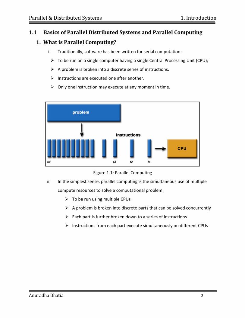
i. Traditionally, software has been written for serial computation:
To be run on a single computer having a single Central Processing Unit (CPU);
A problem is broken into a discrete series of instructions.
Instructions are executed one after another.
Only one instruction may execute at any moment in time.
Figure 1.1: Parallel Computing
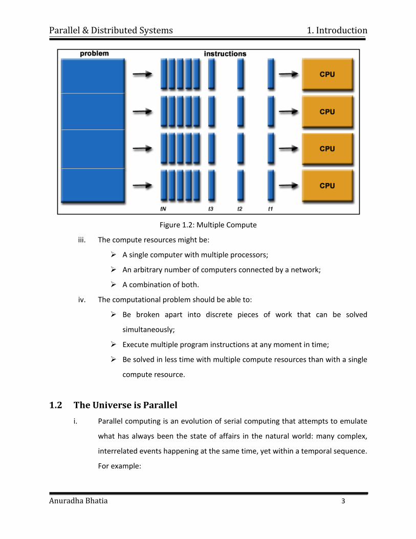
ii. In the simplest sense, parallel computing is the simultaneous use of multiple
compute resources to solve a computational problem:
To be run using multiple CPUs
A problem is broken into discrete parts that can be solved concurrently
Each part is further broken down to a series of instructions
Instructions from each part execute simultaneously on different CPUs
Parallel & Distributed Systems 1. Introduction
Anuradha Bhatia 3
Figure 1.2: Multiple Compute
iii. The compute resources might be:
A single computer with multiple processors;
An arbitrary number of computers connected by a network;
A combination of both.
iv. The computational problem should be able to:
Be broken apart into discrete pieces of work that can be solved
simultaneously;
Execute multiple program instructions at any moment in time;
Be solved in less time with multiple compute resources than with a single
compute resource.
1.2 The Universe is Parallel
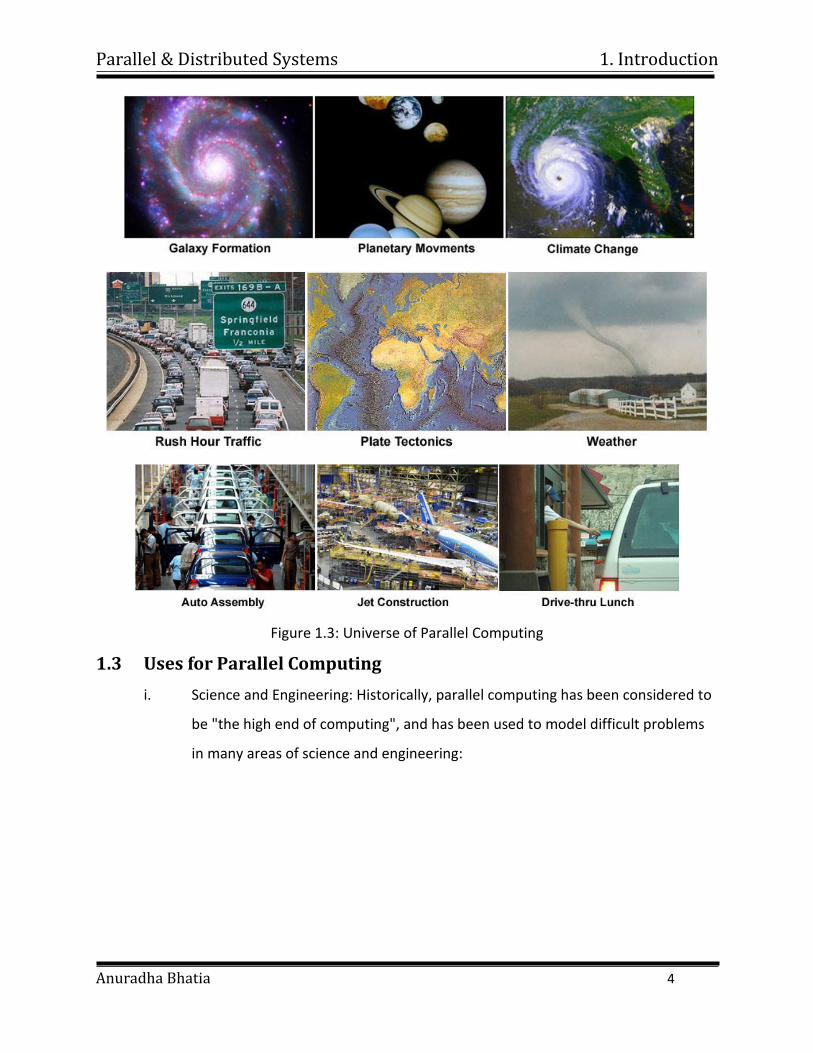
i. Parallel computing is an evolution of serial computing that attempts to emulate
what has always been the state of affairs in the natural world: many complex,
interrelated events happening at the same time, yet within a temporal sequence.
For example:
Parallel & Distributed Systems 1. Introduction
Anuradha Bhatia 4
Figure 1.3: Universe of Parallel Computing
1.3 Uses for Parallel Computing
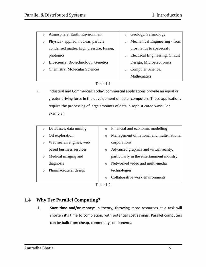
i. Science and Engineering: Historically, parallel computing has been considered to
be "the high end of computing", and has been used to model difficult problems
in many areas of science and engineering:
Parallel & Distributed Systems 1. Introduction
Anuradha Bhatia 5
o Atmosphere, Earth, Environment
o Physics - applied, nuclear, particle,
condensed matter, high pressure, fusion,
photonics
o Bioscience, Biotechnology, Genetics
o Chemistry, Molecular Sciences
o Geology, Seismology
o Mechanical Engineering - from
prosthetics to spacecraft
o Electrical Engineering, Circuit
Design, Microelectronics
o Computer Science,
Mathematics
Table 1.1
ii. Industrial and Commercial: Today, commercial applications provide an equal or
greater driving force in the development of faster computers. These applications
require the processing of large amounts of data in sophisticated ways. For
example:
o Databases, data mining
o Oil exploration
o Web search engines, web
based business services
o Medical imaging and
diagnosis
o Pharmaceutical design
o Financial and economic modelling
o Management of national and multi-national
corporations
o Advanced graphics and virtual reality,
particularly in the entertainment industry
o Networked video and multi-media
technologies
o Collaborative work environments
Table 1.2
1.4 Why Use Parallel Computing?
i. Save time and/or money: In theory, throwing more resources at a task will
shorten it’s time to completion, with potential cost savings. Parallel computers
can be built from cheap, commodity components.
Parallel & Distributed Systems 1. Introduction
Anuradha Bhatia 6
ii. Solve larger problems: Many problems are so large and/or complex that it is
impractical or impossible to solve them on a single computer, especially given
limited computer memory.
iii. Provide concurrency: A single compute resource can only do one thing at a time.
Multiple computing resources can be doing many things simultaneously.
iv. Use of non-local resources: Using compute resources on a wide area network, or
even the Internet when local compute resources are scarce. For example:
v. Limits to serial computing: Both physical and practical reasons pose significant
constraints to simply building ever faster serial computers:
Transmission speeds - the speed of a serial computer is directly dependent
upon how fast data can move through hardware.
Absolute limits are the speed of light (30 cm/nanosecond) and the
transmission limit of copper wire (9 cm/nanosecond).
Increasing speeds necessitate increasing proximity of processing elements.
Limits to miniaturization - processor technology is allowing an increasing
number of transistors to be placed on a chip. However, even with
molecular or atomic-level components, a limit will be reached on how
small components can be.
Economic limitations - it is increasingly expensive to make a single
processor faster. Using a larger number of moderately fast commodity
processors to achieve the same (or better) performance is less expensive.
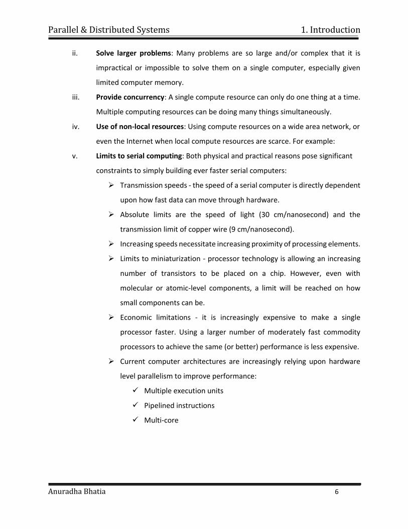
Current computer architectures are increasingly relying upon hardware
level parallelism to improve performance:
Multiple execution units
Pipelined instructions
Multi-core
Parallel & Distributed Systems 1. Introduction
Anuradha Bhatia 7
Figure 1.4: Core Layout
1.5 Concepts and Terminology
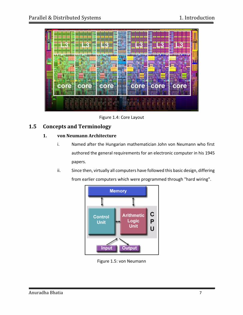
1. von Neumann Architecture
i. Named after the Hungarian mathematician John von Neumann who first
authored the general requirements for an electronic computer in his 1945
papers.
ii. Since then, virtually all computers have followed this basic design, differing
from earlier computers which were programmed through "hard wiring".
Figure 1.5: von Neumann
Parallel & Distributed Systems 1. Introduction
Anuradha Bhatia 8
iii. Comprised of four main components:
Memory
Control Unit
Arithmetic Logic Unit
Input/output
iv. Read/write, random access memory is used to store both program
instructions and data
Program instructions are coded data which tell the computer to
do something
Data is simply information to be used by the program
v. Control unit fetches instructions/data from memory, decodes the
instructions and then sequentially coordinates operations to accomplish
the programmed task.
vi. Arithmetic Unit performs basic arithmetic operations
vii. Input/output is the interface to the human operator.
2. Flynn's Classical Taxonomy
i. One of the more widely used classifications, in use since 1966, is called
Flynn's Taxonomy.
ii. Flynn's taxonomy distinguishes multi-processor computer architectures
according to how they can be classified along the two independent
dimensions of Instruction and Data. Each of these dimensions can have
only one of two possible states: Single or Multiple.
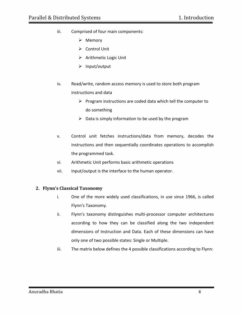
iii. The matrix below defines the 4 possible classifications according to Flynn:
Parallel & Distributed Systems 1. Introduction
Anuradha Bhatia 9
S I S D
Single Instruction, Single Data
S I M D
Single Instruction, Multiple Data
M I S D
Multiple Instruction, Single Data
M I M D
Multiple Instruction, Multiple Data
Figure 1.6: Flynn’s Classical Taxonomy
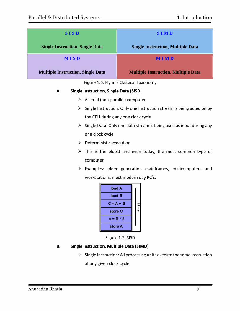
A. Single Instruction, Single Data (SISD)
A serial (non-parallel) computer
Single Instruction: Only one instruction stream is being acted on by
the CPU during any one clock cycle
Single Data: Only one data stream is being used as input during any
one clock cycle
Deterministic execution
This is the oldest and even today, the most common type of
computer
Examples: older generation mainframes, minicomputers and
workstations; most modern day PC’s.
Figure 1.7: SISD
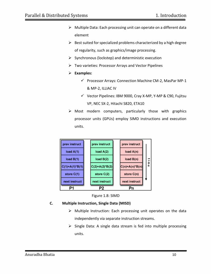
B. Single Instruction, Multiple Data (SIMD)
Single Instruction: All processing units execute the same instruction
at any given clock cycle
Parallel & Distributed Systems 1. Introduction
Anuradha Bhatia 10
Multiple Data: Each processing unit can operate on a different data
element
Best suited for specialized problems characterized by a high degree
of regularity, such as graphics/image processing.
Synchronous (lockstep) and deterministic execution
Two varieties: Processor Arrays and Vector Pipelines
Examples:
Processor Arrays: Connection Machine CM-2, MasPar MP-1
& MP-2, ILLIAC IV
Vector Pipelines: IBM 9000, Cray X-MP, Y-MP & C90, Fujitsu
VP, NEC SX-2, Hitachi S820, ETA10
Most modern computers, particularly those with graphics
processor units (GPUs) employ SIMD instructions and execution
units.
Figure 1.8: SIMD
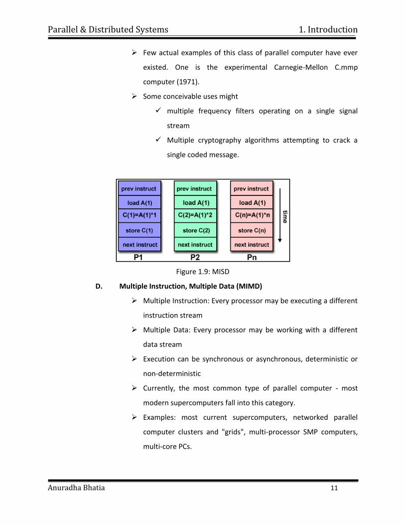
C. Multiple Instruction, Single Data (MISD)
Multiple Instruction: Each processing unit operates on the data
independently via separate instruction streams.
Single Data: A single data stream is fed into multiple processing
units.
Parallel & Distributed Systems 1. Introduction
Anuradha Bhatia 11
Few actual examples of this class of parallel computer have ever
existed. One is the experimental Carnegie-Mellon C.mmp
computer (1971).
Some conceivable uses might
multiple frequency filters operating on a single signal
stream
Multiple cryptography algorithms attempting to crack a
single coded message.
Figure 1.9: MISD
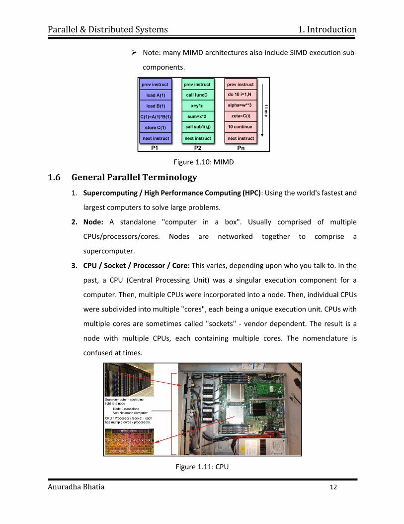
D. Multiple Instruction, Multiple Data (MIMD)
Multiple Instruction: Every processor may be executing a different
instruction stream
Multiple Data: Every processor may be working with a different
data stream
Execution can be synchronous or asynchronous, deterministic or
non-deterministic
Currently, the most common type of parallel computer - most
modern supercomputers fall into this category.
Examples: most current supercomputers, networked parallel
computer clusters and "grids", multi-processor SMP computers,
multi-core PCs.
Parallel & Distributed Systems 1. Introduction
Anuradha Bhatia 12
Note: many MIMD architectures also include SIMD execution sub-
components.
Figure 1.10: MIMD
1.6 General Parallel Terminology
1. Supercomputing / High Performance Computing (HPC): Using the world's fastest and
largest computers to solve large problems.
2. Node: A standalone "computer in a box". Usually comprised of multiple
CPUs/processors/cores. Nodes are networked together to comprise a
supercomputer.
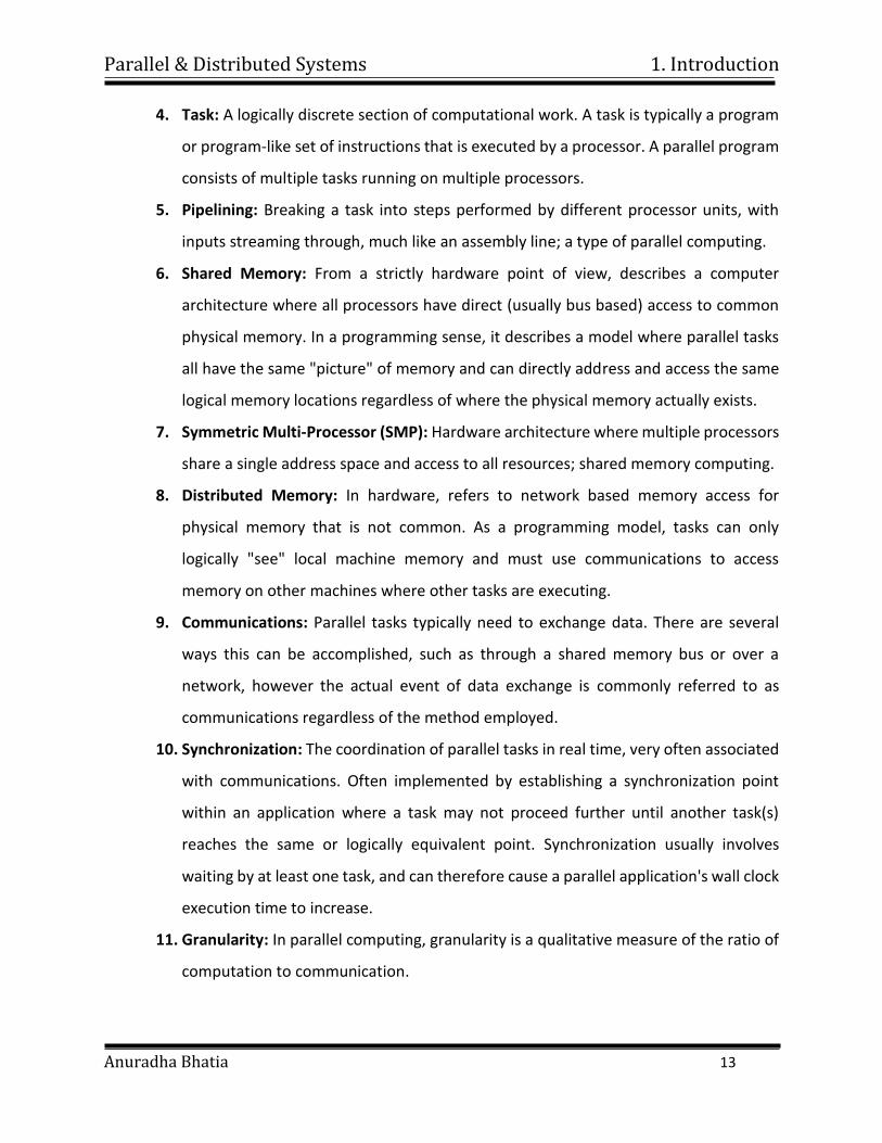
3. CPU / Socket / Processor / Core: This varies, depending upon who you talk to. In the
past, a CPU (Central Processing Unit) was a singular execution component for a
computer. Then, multiple CPUs were incorporated into a node. Then, individual CPUs
were subdivided into multiple "cores", each being a unique execution unit. CPUs with
multiple cores are sometimes called "sockets" - vendor dependent. The result is a
node with multiple CPUs, each containing multiple cores. The nomenclature is
confused at times.
Figure 1.11: CPU
Parallel & Distributed Systems 1. Introduction
Anuradha Bhatia 13
4. Task: A logically discrete section of computational work. A task is typically a program
or program-like set of instructions that is executed by a processor. A parallel program
consists of multiple tasks running on multiple processors.
5. Pipelining: Breaking a task into steps performed by different processor units, with
inputs streaming through, much like an assembly line; a type of parallel computing.
6. Shared Memory: From a strictly hardware point of view, describes a computer
architecture where all processors have direct (usually bus based) access to common
physical memory. In a programming sense, it describes a model where parallel tasks
all have the same "picture" of memory and can directly address and access the same
logical memory locations regardless of where the physical memory actually exists.
7. Symmetric Multi-Processor (SMP): Hardware architecture where multiple processors
share a single address space and access to all resources; shared memory computing.
8. Distributed Memory: In hardware, refers to network based memory access for
physical memory that is not common. As a programming model, tasks can only
logically "see" local machine memory and must use communications to access
memory on other machines where other tasks are executing.
9. Communications: Parallel tasks typically need to exchange data. There are several
ways this can be accomplished, such as through a shared memory bus or over a
network, however the actual event of data exchange is commonly referred to as
communications regardless of the method employed.
10. Synchronization: The coordination of parallel tasks in real time, very often associated
with communications. Often implemented by establishing a synchronization point
within an application where a task may not proceed further until another task(s)
reaches the same or logically equivalent point. Synchronization usually involves
waiting by at least one task, and can therefore cause a parallel application's wall clock
execution time to increase.
11. Granularity: In parallel computing, granularity is a qualitative measure of the ratio of
computation to communication.
Parallel & Distributed Systems 1. Introduction
Anuradha Bhatia 14
12. Coarse: Relatively large amounts of computational work are done between
communication events
13. Fine: Relatively small amounts of computational work are done between
communication events
14. Observed Speedup: Observed speedup of a code which has been parallelized, defined
as:
wall-clock time of serial execution
-----------------------------------
wall-clock time of parallel execution
One of the simplest and most widely used indicators for a parallel program's
performance.
15. Parallel Overhead: The amount of time required to coordinate parallel tasks, as
opposed to doing useful work. Parallel overhead can include factors such as:
Task start-up time
Synchronizations
Data communications
Software overhead imposed by parallel compilers, libraries, tools,
operating system, etc.
Task termination time
16. Massively Parallel: Refers to the hardware that comprises a given parallel system -
having many processors. The meaning of "many" keeps increasing, but currently, the
largest parallel computers can be comprised of processors numbering in the hundreds
of thousands.
17. Embarrassingly Parallel: Solving many similar, but independent tasks simultaneously;
little to no need for coordination between the tasks.
18. Scalability: Refers to a parallel system's (hardware and/or software) ability to
demonstrate a proportionate increase in parallel speedup with the addition of more
processors. Factors that contribute to scalability include:
Parallel & Distributed Systems 1. Introduction
Anuradha Bhatia 15
Hardware - particularly memory-cpu bandwidths and network
communications
Application algorithm
Parallel overhead related
Characteristics of your specific application and coding
1.7 Performance attributes
1. Performance of a system depends upon
i. Hardware technology
ii. Architectural features
iii. Efficient resource management
iv. Algorithm design
v. Data structures
vi. Language efficiency
vii. Programmer skill
viii. Compiler technology
2. Performance of computer system we would describe how quickly a given system can
execute a program or programs. Thus we are interested in knowing the turnaround time.
Turnaround time depends on:
i. Disk and memory accesses
ii. Input and output
iii. Compilation time
iv. Operating system overhead
v. Cpu time
3. An ideal performance of a computer system means a perfect match between the
machine capability and program behavior.
4. The machine capability can be improved by using better hardware technology and
efficient resource management.
Parallel & Distributed Systems 1. Introduction
Anuradha Bhatia 16
5. But as far as program behavior is concerned it depends on code used, compiler
used and other run time conditions. Also a machine performance may vary from
program to program.
6. Because there are too many programs and it is impractical to test a CPU's speed
on all of them, benchmarks were developed. Computer architects have come up
with a variety of metrics to describe the computer performance.
i. Clock rate and CPI / IPC: Since I/O and system overhead frequently overlaps
processing by other programs, it is fair to consider only the CPU time used
by a program, and the user CPU time is the most important factor. CPU is
driven by a clock with a constant cycle time (usually measured in
nanoseconds, which controls the rate of internal operations in the CPU.
The clock mostly has the constant cycle time (t in nanoseconds). The
inverse of the cycle time is the clock rate (f = 1/τ, measured in megahertz).
A shorter clock cycle time, or equivalently a larger number of cycles per
second, implies more operations can be performed per unit time. The size
of the program is determined by the instruction count (Ic). The size of a
program is determined by its instruction count, Ic, the number of machine
instructions to be executed by the program. Different machine instructions
require different numbers of clock cycles to execute. CPI (cycles per
instruction) is thus an important parameter.
ii. MIPS: The millions of instructions per second, this is calculated by dividing
the number of instructions executed in a running program by time
required to run the program. The MIPS rate is directly proportional to the
clock rate and inversely proportion to the CPI. All four systems attributes
(instruction set, compiler, processor, and memory technologies) affect the
MIPS rate, which varies also from program to program. MIPS does not
proved to be effective as it does not account for the fact that different
systems often require different number of instruction to implement the
program. It does not inform about how many instructions are required to
Parallel & Distributed Systems 1. Introduction
Anuradha Bhatia 17
perform a given task. With the variation in instruction styles, internal
organization, and number of processors per system it is almost
meaningless for comparing two systems.
iii. MFLOPS (pronounced ``megaflops'') stands for ``millions of floating point
operations per second.'' This is often used as a ``bottom-line'' figure. If one
know ahead of time how many operations a program needs to perform,
one can divide the number of operations by the execution time to come
up with a MFLOPS rating. For example, the standard algorithm for
multiplying n*n matrices requires 2n3 – n operations (n2 inner products,
with n multiplications and n-1additions in each product). Suppose you
compute the product of two 100 *100 matrices in 0.35 seconds. Then the
computer achieves
(2(100)3 – 100)/0.35 = 5,714,000 ops/sec = 5.714 MFLOPS
iv. Throughput rate: Another important factor on which system’s performance
is measured is throughput of the system which is basically how many
programs a system can execute per unit time Ws. In multiprogramming the
system throughput is often lower than the CPU throughput Wp which is
defined as
Wp = f/(Ic * CPI)
Unit of Wp is programs/second.
v. Speed or Throughput (W/Tn) - the execution rate on an n processor system,
measured in FLOPs/unit-time or instructions/unit-time.
vi. Speedup (Sn = T1/Tn) - how much faster in an actual machine, n processors
compared to
asymptotic speedup.
vii. Efficiency (En = Sn/n) - fraction of the theoretical maximum speedup
achieved by n processors.
viii. Degree of Parallelism (DOP) - for a given piece of the workload, the
number of processors that can be kept busy sharing that piece of
Parallel & Distributed Systems 1. Introduction
Anuradha Bhatia 18
computation equally. Neglecting overhead, we assume that if k processors
work together on any workload, the workload gets done k times as fast as
a sequential execution.
ix. Scalability - The attributes of a computer system which allow it to be
gracefully and linearly scaled up or down in size, to handle smaller or larger
workloads, or to obtain proportional decreases or increase in speed on a
given application. The applications run on a scalable machine may not
scale well. Good scalability requires the algorithm and the machine to have
the right properties
Thus in general there are five performance factors (Ic, p, m, k, t) which are
influenced by four system attributes:
Instruction-set architecture (affects Ic and p)
Compiler technology (affects Ic and p and m)
CPU implementation and control (affects p *t ) cache and memory
hierarchy (affects memory access latency, k ´t)
Total CPU time can be used as a basis in estimating the execution rate
of a processor.
1.8 Parallel Computing Algorithms
i. Parallel algorithms are designed to improve the computation speed of a computer. For
analyzing a Parallel Algorithm, we normally consider the following parameters −
Time complexity (Execution Time),
Total number of processors used, and
Total cost.
Time Complexity
i. The main reason behind developing parallel algorithms was to reduce the
computation time of an algorithm. Thus, evaluating the execution time of an algorithm
is extremely important in analyzing its efficiency.
Parallel & Distributed Systems 1. Introduction
Anuradha Bhatia 19
ii. Execution time is measured on the basis of the time taken by the algorithm to solve a
problem. The total execution time is calculated from the moment when the algorithm
starts executing to the moment it stops. If all the processors do not start or end
execution at the same time, then the total execution time of the algorithm is the
moment when the first processor started its execution to the moment when the last
processor stops its execution.
iii. Time complexity of an algorithm can be classified into three categories−
Worst-case complexity − When the amount of time required by an algorithm
for a given input is maximum.
Average-case complexity − When the amount of time required by an algorithm
for a given input is average.
Best-case complexity − When the amount of time required by an algorithm for
a given input is minimum.
Asymptotic Analysis
i. The complexity or efficiency of an algorithm is the number of steps executed by the
algorithm to get the desired output. Asymptotic analysis is done to calculate the
complexity of an algorithm in its theoretical analysis. In asymptotic analysis, a large
length of input is used to calculate the complexity function of the algorithm.
ii. Note − Asymptotic is a condition where a line tends to meet a curve, but they do not
intersect. Here the line and the curve is asymptotic to each other.
iii. Asymptotic notation is the easiest way to describe the fastest and slowest possible
execution time for an algorithm using high bounds and low bounds on speed. For this,
we use the following notations −
Big O notation
Omega notation
Theta notation
Parallel & Distributed Systems 1. Introduction
Anuradha Bhatia 20
Big O notation
In mathematics, Big O notation is used to represent the asymptotic characteristics of
functions. It represents the behavior of a function for large inputs in a simple and
accurate method. It is a method of representing the upper bound of an algorithm’s
execution time. It represents the longest amount of time that the algorithm could take
to complete its execution. The function −
f(n) = O(g(n))
if there exists positive constants c and n0 such that f(n) ≤ c * g(n) for all n where n ≥
n0.
Omega notation
Omega notation is a method of representing the lower bound of an algorithm’s
execution time. The function −
f(n) = Ω (g(n))
if there exists positive constants c and n0 such that f(n) ≥ c * g(n) for all n where n ≥
n0.
Theta Notation
Theta notation is a method of representing both the lower bound and the upper bound
of an algorithm’s execution time. The function −
f(n) = θ(g(n))
if there exists positive constants c1, c2, and n0 such that c1 * g(n) ≤ f(n) ≤ c2 * g(n) for
all n where n ≥ n0.
1.9 Parallel Computing Algorithms Models
1. The Data-Parallel Model
i. The data-parallel model is one of the simplest algorithm models. In this
model, the tasks are statically or semi-statically mapped onto processes
and each task performs similar operations on different data.
ii. This type of parallelism that is a result of identical operations being applied
concurrently on different data items is called data parallelism.
Parallel & Distributed Systems 1. Introduction
Anuradha Bhatia 21
iii. The work may be done in phases and the data operated upon in different
phases may be different.
iv. Typically, data-parallel computation phases are interspersed with
interactions to synchronize the tasks or to get fresh data to the tasks.
v. Since all tasks perform similar computations, the decomposition of the
problem into tasks is usually based on data partitioning because a uniform
partitioning of data followed by a static mapping is sufficient to guarantee
load balance.
vi. Data-parallel algorithms can be implemented in both shared-address-
space and message-passing paradigms.
vii. The partitioned address-space in a message-passing paradigm may allow
better control of placement, and thus may offer a better handle on locality.
viii. On the other hand, shared-address space can ease the programming
effort, especially if the distribution of data is different in different phases
of the algorithm.
ix. Interaction overheads in the data-parallel model can be minimized by
choosing a locality preserving decomposition and, if applicable, by
overlapping computation and interaction and by using optimized collective
interaction routines.
x. A key characteristic of data-parallel problems is that for most problems,
the degree of data parallelism increases with the size of the problem,
making it possible to use more processes to effectively solve larger
problems.
2. The Task Graph Model
i. The computations in any parallel algorithm can be viewed as a task-
dependency graph.
ii. The task-dependency graph may be either trivial, as in the case of matrix
multiplication, or nontrivial However, in certain parallel algorithms, the
task-dependency graph is explicitly used in mapping. In the task graph
Parallel & Distributed Systems 1. Introduction
Anuradha Bhatia 22
model, the interrelationships among the tasks are utilized to promote
locality or to reduce interaction costs.
iii. This model is typically employed to solve problems in which the amount of
data associated with the tasks is large relative to the amount of
computation associated with them.
iv. Usually, tasks are mapped statically to help optimize the cost of data
movement among tasks.
v. Sometimes a decentralized dynamic mapping may be used, but even then,
the mapping uses the information about the task-dependency graph
structure and the interaction pattern of tasks to minimize interaction
overhead.
vi. Work is more easily shared in paradigms with globally addressable space,
but mechanisms are available to share work in disjoint address space.
vii. Typical interaction-reducing techniques applicable to this model include
reducing the volume and frequency of interaction by promoting locality
while mapping the tasks based on the interaction pattern of tasks, and
using asynchronous interaction methods to overlap the interaction with
computation.
viii. Examples of algorithms based on the task graph model include parallel
quicksort sparse matrix factorization, and many parallel algorithms derived
via divide-and-conquer decomposition.
ix. This type of parallelism that is naturally expressed by independent tasks in
a task-dependency graph is called task parallelism.
3. The Work Pool Model
i. The work pool or the task pool model is characterized by a dynamic
mapping of tasks onto processes for load balancing in which any task may
potentially be performed by any process.
ii. There is no desired premapping of tasks onto processes. The mapping may
be centralized or decentralized. Pointers to the tasks may be stored in a
Parallel & Distributed Systems 1. Introduction
Anuradha Bhatia 23
physically shared list, priority queue, hash table, or tree, or they could be
stored in a physically distributed data structure.
iii. The work may be statically available in the beginning, or could be
dynamically generated; i.e., the processes may generate work and add it
to the global (possibly distributed) work pool.
iv. If the work is generated dynamically and a decentralized mapping is used,
then a termination detection algorithm (In the message-passing paradigm,
the work pool model is typically used when the amount of data associated
with tasks is relatively small compared to the computation associated with
the tasks. As a result, tasks can be readily moved around without causing
too much data interaction overhead.
v. The granularity of the tasks can be adjusted to attain the desired level of
tradeoff between load-imbalance and the overhead of accessing the work
pool for adding and extracting tasks.
vi. Parallelization of loops by chunk scheduling or related methods is an
example of the use of the work pool model with centralized mapping when
the tasks are statically available.
vii. Parallel tree search where the work is represented by a centralized or
distributed data structure is an example of the use of the work pool model
where the tasks are generated dynamically.
4. The Master-Slave Model
i. In the master-slave or the manager-worker model, one or more master
processes generate work and allocate it to worker processes.
ii. The tasks may be allocated a priori if the manager can estimate the size of
the tasks or if a random mapping can do an adequate job of load balancing.
In another scenario, workers are assigned smaller pieces of work at
different times.
Parallel & Distributed Systems 1. Introduction
Anuradha Bhatia 24
iii. The latter scheme is preferred if it is time consuming for the master to
generate work and hence it is not desirable to make all workers wait until
the master has generated all work pieces.
iv. In some cases, work may need to be performed in phases, and work in
each phase must finish before work in the next phases can be generated.
In this case, the manager may cause all workers to synchronize after each
phase.
v. Usually, there is no desired premapping of work to processes, and any
worker can do any job assigned to it. The manager-worker model can be
generalized to the hierarchical or multi-level manager-worker model in
which the top-level manager feeds large chunks of tasks to second-level
managers, who further subdivide the tasks among their own workers and
may perform part of the work themselves.
vi. This model is generally equally suitable to shared-address-space or
message-passing paradigms since the interaction is naturally two-way; i.e.,
the manager knows that it needs to give out work and workers know that
they need to get work from the manager.
vii. While using the master-slave model, care should be taken to ensure that
the master does not become a bottleneck, which may happen if the tasks
are too small (or the workers are relatively fast).
viii. The granularity of tasks should be chosen such that the cost of doing work
dominates the cost of transferring work and the cost of synchronization.
ix. Asynchronous interaction may help overlap interaction and the
computation associated with work generation by the master. It may also
reduce waiting times if the nature of requests from workers is non-
deterministic.
5. The Pipeline or Producer-Consumer Model
i. In the pipeline model, a stream of data is passed on through a succession
of processes, each of which perform some task on it.
Parallel & Distributed Systems 1. Introduction
Anuradha Bhatia 25
ii. This simultaneous execution of different programs on a data stream is
called stream parallelism.
iii. With the exception of the process initiating the pipeline, the arrival of new
data triggers the execution of a new task by a process in the pipeline. The
processes could form such pipelines in the shape of linear or
multidimensional arrays, trees, or general graphs with or without cycles.
iv. A pipeline is a chain of producers and consumers. Each process in the
pipeline can be viewed as a consumer of a sequence of data items for the
process preceding it in the pipeline and as a producer of data for the
process following it in the pipeline.
v. The pipeline does not need to be a linear chain; it can be a directed graph.
The pipeline model usually involves a static mapping of tasks onto
processes.
vi. Load balancing is a function of task granularity. The larger the granularity,
the longer it takes to fill up the pipeline, i.e. for the trigger produced by the
first process in the chain to propagate to the last process, thereby keeping
some of the processes waiting.
vii. However, too fine a granularity may increase interaction overheads
because processes will need to interact to receive fresh data after smaller
pieces of computation. The most common interaction reduction technique
applicable to this model is overlapping interaction with computation.
6. Hybrid Models
i. In some cases, more than one model may be applicable to the problem at
hand, resulting in a hybrid algorithm model.
ii. A hybrid model may be composed either of multiple models applied
hierarchically or multiple models applied sequentially to different phases
of a parallel algorithm. In some cases, an algorithm formulation may have
characteristics of more than one algorithm model.
Parallel & Distributed Systems 1. Introduction
Anuradha Bhatia 26
iii. For instance, data may flow in a pipelined manner in a pattern guided by a
task-dependency graph. In another scenario, the major computation may
be described by a task-dependency graph, but each node of the graph may
represent a super task comprising multiple subtasks that may be suitable
for data-parallel or pipelined parallelism.
1.10 Parallel Programming Models
i. There are several parallel programming models in common use:
Shared Memory (without threads)
Threads
Distributed Memory / Message Passing
Data Parallel
Hybrid
Single Program Multiple Data (SPMD)
Multiple Program Multiple Data (MPMD)
ii. Parallel programming models exist as an abstraction above hardware and
memory architectures.
iii. Although it might not seem apparent, these models are NOT specific to a
particular type of machine or memory architecture. In fact, any of these
models can (theoretically) be implemented on any underlying hardware.
Two examples from the past are discussed below.
iv. SHARED memory model on a DISTRIBUTED memory machine: Kendall
Square Research (KSR) ALLCACHE approach.
v. Machine memory was physically distributed across networked machines,
but appeared to the user as a single shared memory (global address space).
Generically, this approach is referred to as "virtual shared memory".
vi. DISTRIBUTED memory model on a SHARED memory machine: Message
Passing Interface (MPI) on SGI Origin 2000.
vii. The SGI Origin 2000 employed the CC-NUMA type of shared memory
architecture, where every task has direct access to global address space
Parallel & Distributed Systems 1. Introduction
Anuradha Bhatia 27
spread across all machines. However, the ability to send and receive
messages using MPI, as is commonly done over a network of distributed
memory machines, was implemented and commonly used.
1. Shared Memory Model (without threads)
i. In this programming model, tasks share a common address space, which
they read and write to asynchronously.
ii. Various mechanisms such as locks / semaphores may be used to control
access to the shared memory.
iii. An advantage of this model from the programmer's point of view is that
the notion of data "ownership" is lacking, so there is no need to specify
explicitly the communication of data between tasks. Program
development can often be simplified.
iv. An important disadvantage in terms of performance is that it becomes
more difficult to understand and manage data locality.
Keeping data local to the processor that works on it conserves memory
accesses, cache refreshes and bus traffic that occurs when multiple
processors use the same data.
Unfortunately, controlling data locality is hard to understand and
beyond the control of the average user.
v. Implementation: Native compilers and/or hardware translate user
program variables into actual memory addresses, which are global. On
stand-alone SMP machines, this is straightforward.
vi. On distributed shared memory machines, such as the SGI Origin, memory
is physically distributed across a network of machines, but made global
through specialized hardware and software.
2. Threads Model
i. This programming model is a type of shared memory programming.
ii. In the threads model of parallel programming, a single process can have
multiple, concurrent execution paths.
Parallel & Distributed Systems 1. Introduction
Anuradha Bhatia 28
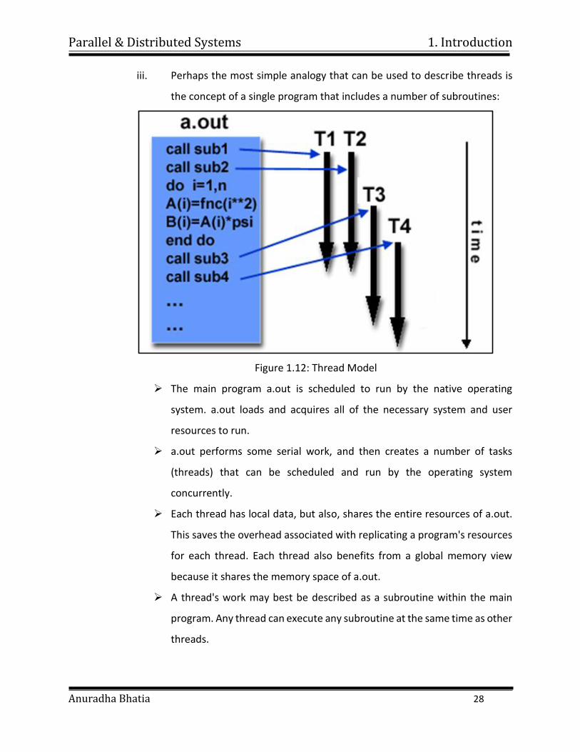
iii. Perhaps the most simple analogy that can be used to describe threads is
the concept of a single program that includes a number of subroutines:
Figure 1.12: Thread Model
The main program a.out is scheduled to run by the native operating
system. a.out loads and acquires all of the necessary system and user
resources to run.
a.out performs some serial work, and then creates a number of tasks
(threads) that can be scheduled and run by the operating system
concurrently.
Each thread has local data, but also, shares the entire resources of a.out.
This saves the overhead associated with replicating a program's resources
for each thread. Each thread also benefits from a global memory view
because it shares the memory space of a.out.
A thread's work may best be described as a subroutine within the main
program. Any thread can execute any subroutine at the same time as other
threads.
Parallel & Distributed Systems 1. Introduction
Anuradha Bhatia 29
Threads communicate with each other through global memory (updating
address locations). This requires synchronization constructs to ensure that
more than one thread is not updating the same global address at any time.
Threads can come and go, but a.out remains present to provide the
necessary shared resources until the application has completed.
iv. Implementation: From a programming perspective, threads
implementations commonly comprise:
v. A library of subroutines that are called from within parallel source code
vi. A set of compiler directives imbedded in either serial or parallel source
code
vii. Threaded implementations are not new in computing. Historically,
hardware vendors have implemented their own proprietary versions of
threads. These implementations differed substantially from each other
making it difficult for programmers to develop portable threaded
applications.
viii. Unrelated standardization efforts have resulted in two very different
implementations of threads: POSIX Threads and OpenMP.
ix. POSIX Threads
Library based; requires parallel coding
Specified by the IEEE POSIX 1003.1c standard (1995).
C Language only
Commonly referred to as Pthreads.
Most hardware vendors now offer Pthreads in addition to their
proprietary threads implementations.
Very explicit parallelism; requires significant programmer attention
to detail.
x. OpenMP
Compiler directive based; can use serial code
Parallel & Distributed Systems 1. Introduction
Anuradha Bhatia 30
Jointly defined and endorsed by a group of major computer
hardware and software vendors. The OpenMP Fortran API was
released October 28, 1997. The C/C++ API was released in late
1998.
Portable / multi-platform, including Unix and Windows NT
platforms
Available in C/C++ and Fortran implementations
Can be very easy and simple to use - provides for "incremental
parallelism"
Microsoft has its own implementation for threads, which is not
related to the UNIX POSIX standard or OpenMP.
3. Distributed Memory / Message Passing Model
i. This model demonstrates the following characteristics:
ii. A set of tasks that use their own local memory during computation.
Multiple tasks can reside on the same physical machine and/or across an
arbitrary number of machines.
Tasks exchange data through communications by sending and
receiving messages.
Data transfer usually requires cooperative operations to be
performed by each process. For example, a send operation must
have a matching receive operation.
Parallel & Distributed Systems 1. Introduction
Anuradha Bhatia 31
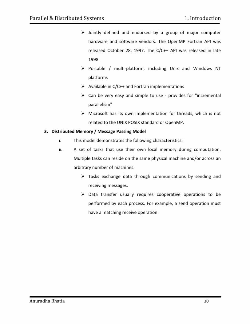
Figure 1.13: Message Passing Model
Tasks exchange data through communications by sending and
receiving messages.
Data transfer usually requires cooperative operations to be
performed by each process. For example, a send operation must
have a matching receive operation.
iii. From a programming perspective, message passing implementations
usually comprise a library of subroutines. Calls to these subroutines are
imbedded in source code. The programmer is responsible for determining
all parallelism.
iv. Historically, a variety of message passing libraries have been available
since the 1980s. These implementations differed substantially from each
other making it difficult for programmers to develop portable applications.
v. In 1992, the MPI Forum was formed with the primary goal of establishing
a standard interface for message passing implementations.
vi. Part 1 of the Message Passing Interface (MPI) was released in 1994. Part
2 (MPI-2) was released in 1996.
Parallel & Distributed Systems 1. Introduction
Anuradha Bhatia 32
vii. MPI is now the "de facto" industry standard for message passing, replacing
virtually all other message passing implementations used for production
work. MPI implementations exist for virtually all popular parallel
computing platforms. Not all implementations include everything in both
MPI1 and MPI2.
4. Data Parallel Model
i. The data parallel model demonstrates the following characteristics:
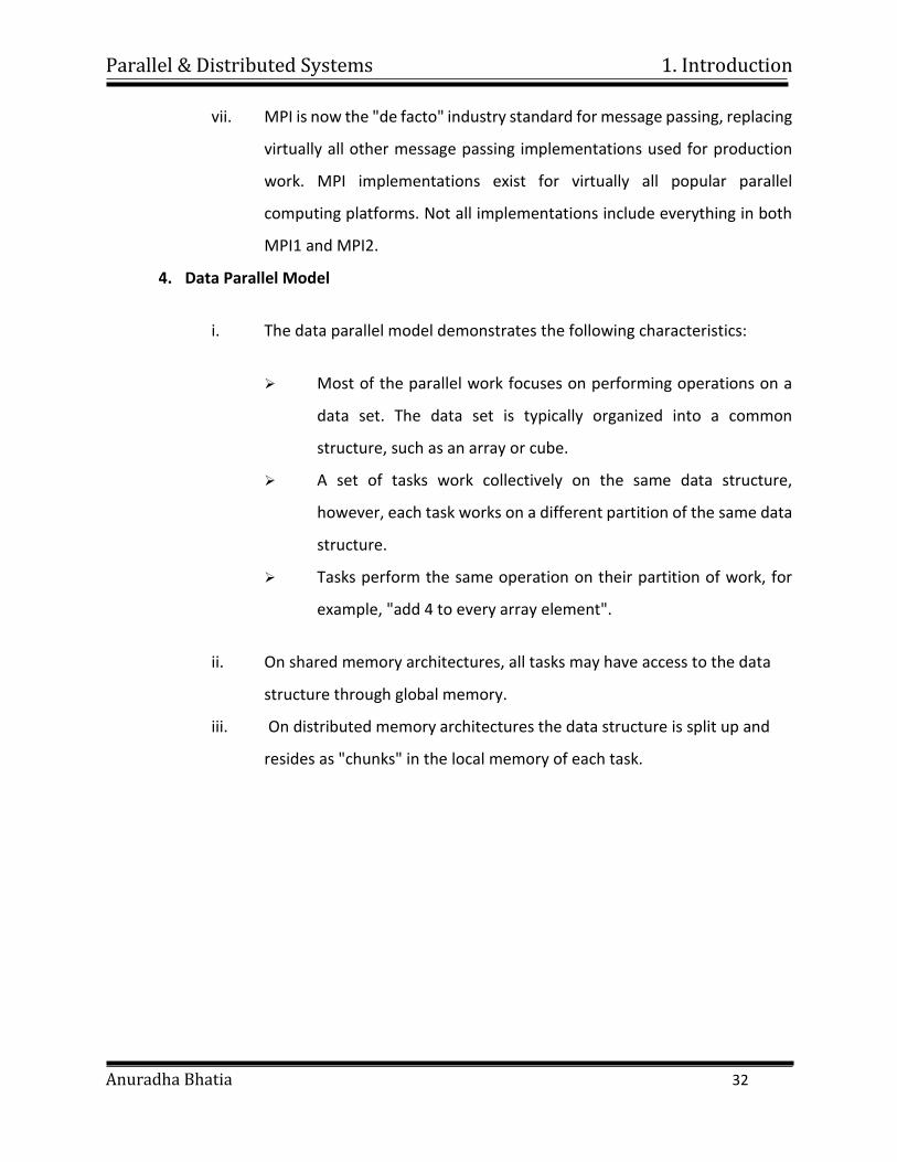
Most of the parallel work focuses on performing operations on a
data set. The data set is typically organized into a common
structure, such as an array or cube.
A set of tasks work collectively on the same data structure,
however, each task works on a different partition of the same data
structure.
Tasks perform the same operation on their partition of work, for
example, "add 4 to every array element".
ii. On shared memory architectures, all tasks may have access to the data
structure through global memory.
iii. On distributed memory architectures the data structure is split up and
resides as "chunks" in the local memory of each task.
Parallel & Distributed Systems 1. Introduction
Anuradha Bhatia 33
Figure 1.14: Data Parallel Model
iv. Implementations:
Programming with the data parallel model is usually accomplished by
writing a program with data parallel constructs. The constructs can be
calls to a data parallel subroutine library or, compiler directives
recognized by a data parallel compiler.
FORTRAN 90 and 95 (F90, F95): ISO/ANSI standard extensions to Fortran
77.
Contains everything that is in Fortran 77
New source code format; additions to character set
Additions to program structure and commands
Variable additions - methods and arguments
Pointers and dynamic memory allocation added
Parallel & Distributed Systems 1. Introduction
Anuradha Bhatia 34
Array processing (arrays treated as objects) added
Recursive and new intrinsic functions added
Many other new features
High Performance FORTRAN (HPF): Extensions to Fortran 90 to support
data parallel programming.
Contains everything in Fortran 90
Directives to tell compiler how to distribute data added
Assertions that can improve optimization of generated code
added
Data parallel constructs added (now part of Fortran 95)
HPF compilers were relatively common in the 1990s, but are no longer
commonly implemented.
Compiler Directives: Allow the programmer to specify the distribution
and alignment of data. FORTRAN implementations are available for most
common parallel platforms.
Distributed memory implementations of this model usually require the
compiler to produce object code with calls to a message passing library
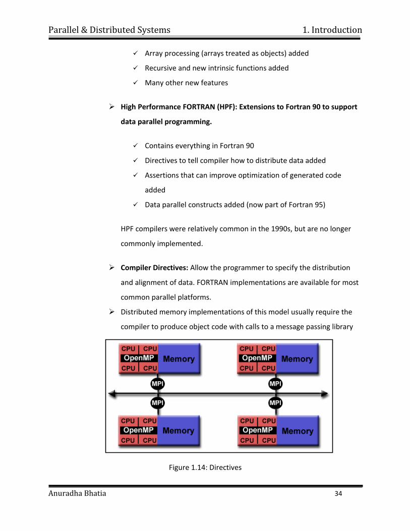
Figure 1.14: Directives
Parallel & Distributed Systems 1. Introduction
Anuradha Bhatia 35
(MPI) for data distribution. All message passing is done invisibly to the
programmer.
5. Hybrid Model
i. A hybrid model combines more than one of the previously described
programming models.
ii. Currently, a common example of a hybrid model is the combination of the
message passing model (MPI) with the threads model (OpenMP).
Threads perform computationally intensive kernels using local, on-
node data
Communications between processes on different nodes occurs over
the network using MPI
iii. This hybrid model lends itself well to the increasingly common hardware
environment of clustered multi/many-core machines.
iv. Another similar and increasingly popular example of a hybrid model is
using MPI with GPU (Graphics Processing Unit) programming.
GPUs perform computationally intensive kernels using local, on-node
data
Communications between processes on different nodes occurs over
sthe network using MPI
Parallel & Distributed Systems
Anuradha Bhatia
2. Pipeline Processing
CONTENTS
2.1 Introduction
2.2 Pipeline Performance
2.3 Arithmetic Pipelines
2.4 Pipelined Instruction Processing
2.5 Pipeline Stage Design
2.6 Hazards, Dynamic
2.7 Instruction Scheduling
Parallel & Distributed Systems 2. Pipeline Processing
Anuradha Bhatia 37
2.1 Introduction
1. Pipelining is one way of improving the overall processing performance of a processor.
2. This architectural approach allows the simultaneous execution of several instructions.
3. Pipelining is transparent to the programmer; it exploits parallelism at the instruction
level by overlapping the execution process of instructions.
4. It is analogous to an assembly line where workers perform a specific task and pass the
partially completed product to the next worker.
2.2 Pipeline Structure
1. The pipeline design technique decomposes a sequential process into several sub
processes, called stages or segments.
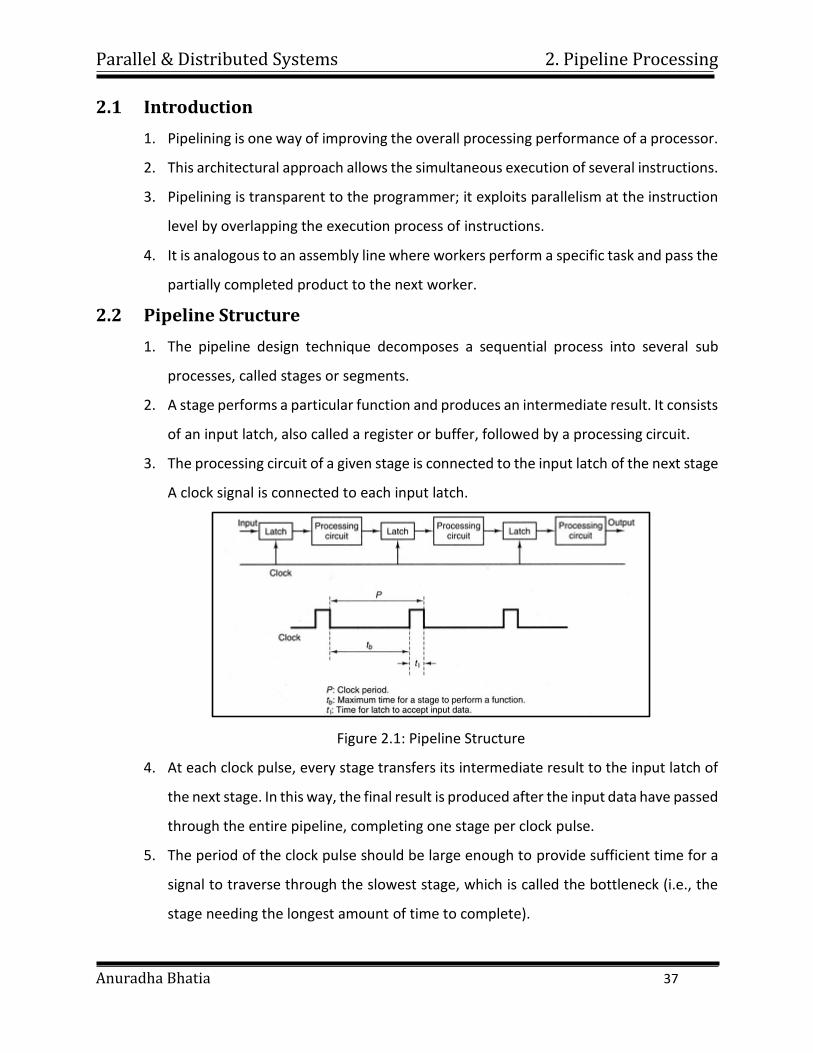
2. A stage performs a particular function and produces an intermediate result. It consists
of an input latch, also called a register or buffer, followed by a processing circuit.
3. The processing circuit of a given stage is connected to the input latch of the next stage
A clock signal is connected to each input latch.
Figure 2.1: Pipeline Structure
4. At each clock pulse, every stage transfers its intermediate result to the input latch of
the next stage. In this way, the final result is produced after the input data have passed
through the entire pipeline, completing one stage per clock pulse.
5. The period of the clock pulse should be large enough to provide sufficient time for a
signal to traverse through the slowest stage, which is called the bottleneck (i.e., the
stage needing the longest amount of time to complete).
Parallel & Distributed Systems 2. Pipeline Processing
Anuradha Bhatia 38
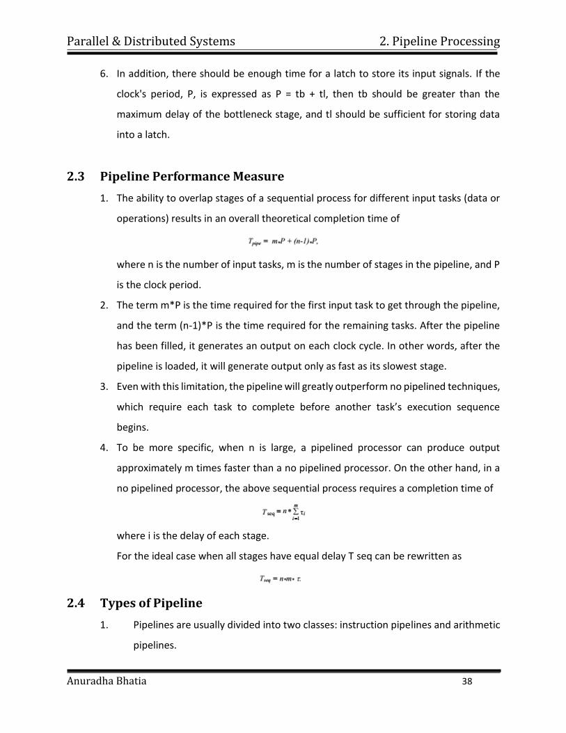
6. In addition, there should be enough time for a latch to store its input signals. If the
clock's period, P, is expressed as P = tb + tl, then tb should be greater than the
maximum delay of the bottleneck stage, and tl should be sufficient for storing data
into a latch.
2.3 Pipeline Performance Measure
1. The ability to overlap stages of a sequential process for different input tasks (data or
operations) results in an overall theoretical completion time of
where n is the number of input tasks, m is the number of stages in the pipeline, and P
is the clock period.
2. The term m*P is the time required for the first input task to get through the pipeline,
and the term (n-1)*P is the time required for the remaining tasks. After the pipeline
has been filled, it generates an output on each clock cycle. In other words, after the
pipeline is loaded, it will generate output only as fast as its slowest stage.
3. Even with this limitation, the pipeline will greatly outperform no pipelined techniques,
which require each task to complete before another task’s execution sequence
begins.
4. To be more specific, when n is large, a pipelined processor can produce output
approximately m times faster than a no pipelined processor. On the other hand, in a
no pipelined processor, the above sequential process requires a completion time of
where i is the delay of each stage.
For the ideal case when all stages have equal delay T seq can be rewritten as
2.4 Types of Pipeline
1. Pipelines are usually divided into two classes: instruction pipelines and arithmetic
pipelines.
Parallel & Distributed Systems 2. Pipeline Processing
Anuradha Bhatia 39
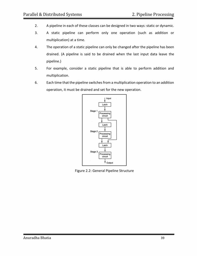
2. A pipeline in each of these classes can be designed in two ways: static or dynamic.
3. A static pipeline can perform only one operation (such as addition or
multiplication) at a time.
4. The operation of a static pipeline can only be changed after the pipeline has been
drained. (A pipeline is said to be drained when the last input data leave the
pipeline.)
5. For example, consider a static pipeline that is able to perform addition and
multiplication.
6. Each time that the pipeline switches from a multiplication operation to an addition
operation, it must be drained and set for the new operation.
Figure 2.2: General Pipeline Structure
Parallel & Distributed Systems 2. Pipeline Processing
Anuradha Bhatia 40
2.5 Arithmetic Pipelining
1. The pipeline structures used for instruction pipelining may be applied in some cases
to other processing tasks.
2. If pipelining is to be useful, however, we must be faced with the need to perform a
long sequence of essentially similar tasks.
3. Large numerical applications often make use of repeated arithmetic operations for
processing the elements of vectors and arrays.
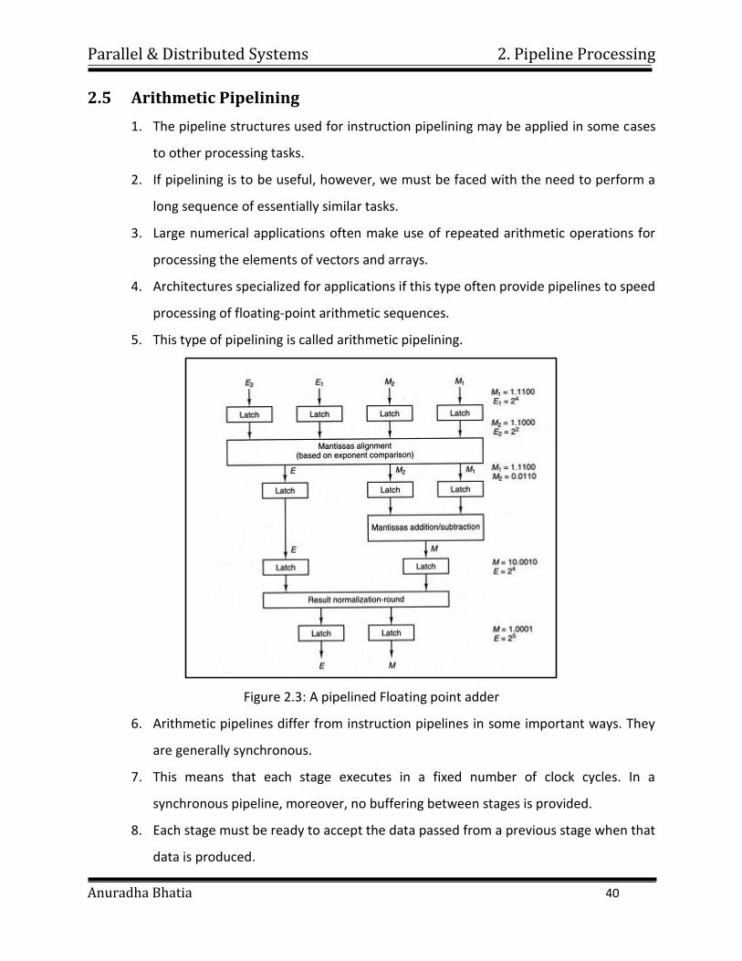
4. Architectures specialized for applications if this type often provide pipelines to speed
processing of floating-point arithmetic sequences.
5. This type of pipelining is called arithmetic pipelining.
Figure 2.3: A pipelined Floating point adder
6. Arithmetic pipelines differ from instruction pipelines in some important ways. They
are generally synchronous.
7. This means that each stage executes in a fixed number of clock cycles. In a
synchronous pipeline, moreover, no buffering between stages is provided.
8. Each stage must be ready to accept the data passed from a previous stage when that
data is produced.
Parallel & Distributed Systems 2. Pipeline Processing
Anuradha Bhatia 41
2.6 Instruction pipelining
1. In order to speed up the operation of a computer system beyond what is possible with
sequential execution, methods must be found to perform more than one task at a
time.
2. One method for gaining significant speedup with modest hardware cost is the
technique of pipelining.
3. In this technique, A task is broken down into multiple steps, and independent
processing units are assigned to each step. Once a task has completed its initial step,
another task may enter that step while the original task moves on to the following
step.
4. The process is much like an assembly line, with a different task in progress at each
stage. In theory, a pipeline which breaks a process into N steps could achieve an N-
fold increase in processing speed. Due to various practical problems, the actual gain
may be significantly less.
5. The concept of pipelines can be extended to various structures of interconnected
processing elements, including those in which data flows from more than one source
or to more than one destination, or may be fed back into an earlier stage.
6. We will limit our attention to linear sequential pipelines in which all data flows
through the stages in the same sequence, and data remains in the same order in which
it originally entered.
7. Pipelining is most suited for tasks in which essentially the same sequence of steps
must be repeated many times for different data.
Parallel & Distributed Systems 2. Pipeline Processing
Anuradha Bhatia 42
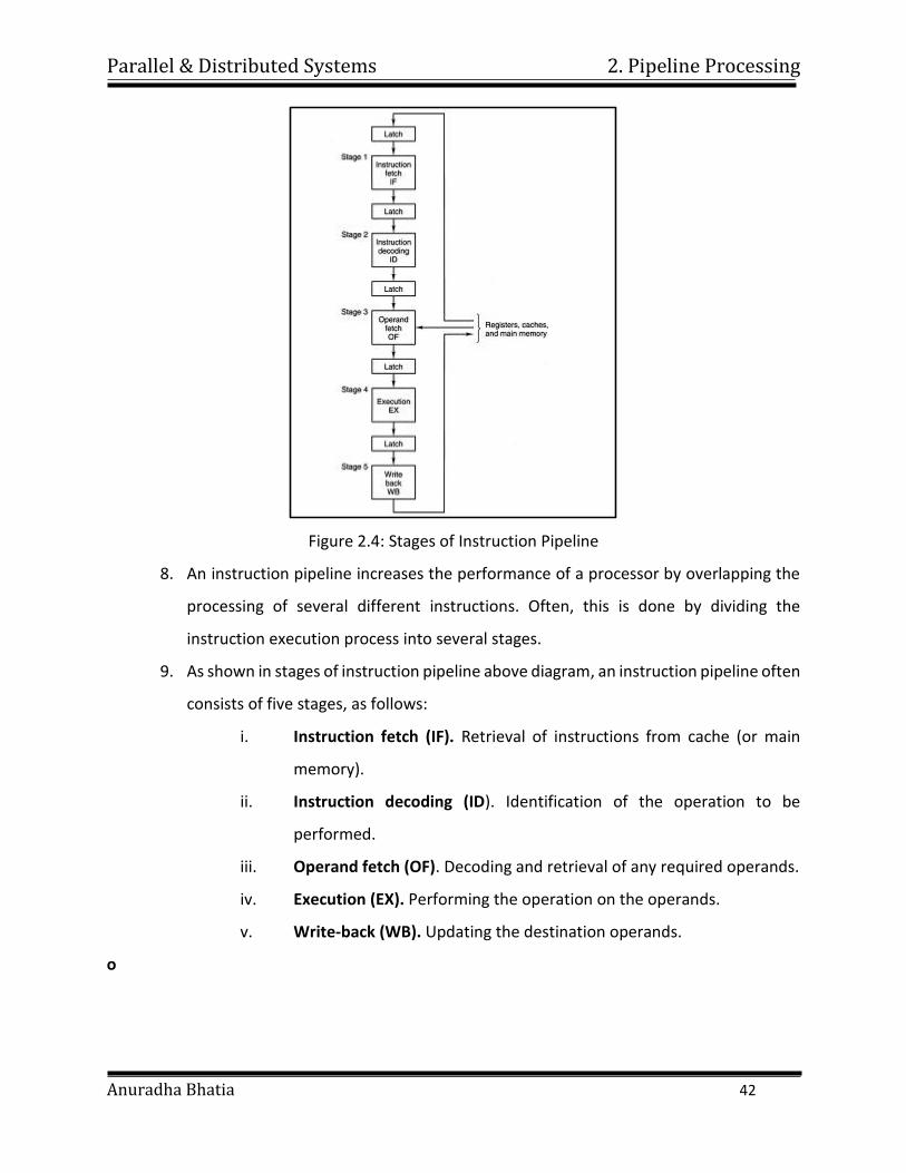
Figure 2.4: Stages of Instruction Pipeline
8. An instruction pipeline increases the performance of a processor by overlapping the
processing of several different instructions. Often, this is done by dividing the
instruction execution process into several stages.
9. As shown in stages of instruction pipeline above diagram, an instruction pipeline often
consists of five stages, as follows:
i. Instruction fetch (IF). Retrieval of instructions from cache (or main
memory).
ii. Instruction decoding (ID). Identification of the operation to be
performed.
iii. Operand fetch (OF). Decoding and retrieval of any required operands.
iv. Execution (EX). Performing the operation on the operands.
v. Write-back (WB). Updating the destination operands.
o
Parallel & Distributed Systems 2. Pipeline Processing
Anuradha Bhatia 43
2.7 Instruction Processing
1. The first step in applying pipelining techniques to instruction processing is to divide
the task into steps that may be performed with independent hardware.
2. The most obvious division is between the FETCH cycle (fetch and interpret
instructions) and the EXECUTE cycle (access operands and perform operation).
3. If these two activities are to run simultaneously, they must use independent registers
and processing circuits, including independent access to memory (separate MAR and
MBR).
4. It is possible to further divide FETCH into fetching and interpreting, but since
interpreting is very fast this is not generally done.
5. To gain the benefits of pipelining it is desirable that each stage take a comparable
amount of time.
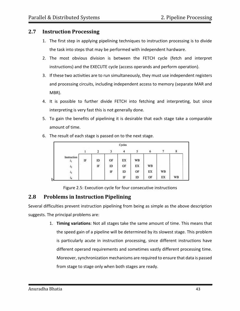
6. The result of each stage is passed on to the next stage.
b
Figure 2.5: Execution cycle for four consecutive instructions
2.8 Problems in Instruction Pipelining
Several difficulties prevent instruction pipelining from being as simple as the above description
suggests. The principal problems are:
1. Timing variations: Not all stages take the same amount of time. This means that
the speed gain of a pipeline will be determined by its slowest stage. This problem
is particularly acute in instruction processing, since different instructions have
different operand requirements and sometimes vastly different processing time.
Moreover, synchronization mechanisms are required to ensure that data is passed
from stage to stage only when both stages are ready.
Parallel & Distributed Systems 2. Pipeline Processing
Anuradha Bhatia 44
2. Data hazards: When several instructions are in partial execution, a problem arises
if they reference the same data. We must ensure that a later instruction does not
attempt to access data sooner than a preceding instruction, if this will lead to
incorrect results. For example, instruction N+1 must not be permitted to fetch an
operand that is yet to be stored into by instruction N.
3. Branching: In order to fetch the "next" instruction, we must know which one is
required. If the present instruction is a conditional branch, the next instruction
may not be known until the current one is processed.
4. Interrupts: Interrupts insert unplanned "extra" instructions into the instruction
stream. The interrupt must take effect between instructions, that is, when one
instruction has completed and the next has not yet begun. With pipelining, the
next instruction has usually begun before the current one has completed.
Possible solutions to the problems described above include the following strategies:
1. Timing Variations: To maximize the speed gain, stages must first be chosen to be as
uniform as possible in timing requirements. However, a timing mechanism is needed.
A synchronous method could be used, in which a stage is assumed to be complete in
a definite number of clock cycles. However, asynchronous techniques are generally
more efficient. A flag bit or signal line is passed forward to the next stage indicating
when valid data is available. A signal must also be passed back from the next stage
when the data has been accepted. In all cases there must be a buffer register between
stages to hold the data; sometimes this buffer is expanded to a memory which can
hold several data items. Each stage must take care not to accept input data until it is
valid, and not to produce output data until there is room in its output buffer.
2. Data Hazards: To guard against data hazards it is necessary for each stage to be aware
of the operands in use by stages further down the pipeline. The type of use must also
be known, since two successive reads do not conflict and should not be cause to slow
the pipeline. Only when writing is involved is there a possible conflict. The pipeline is
typically equipped with a small associative check memory which can store the address
and operation type (read or write) for each instruction currently in the pipe. The
Parallel & Distributed Systems 2. Pipeline Processing
Anuradha Bhatia 45
concept of "address" must be extended to identify registers as well. Each instruction
can affect only a small number of operands, but indirect effects of addressing must
not be neglected.
3. Branching: The problem in branching is that the pipeline may be slowed down by a
branch instruction because we do not know which branch to follow. In the absence of
any special help in this area, it would be necessary to delay processing of further
instructions until the branch destination is resolved. Since branches are extremely
frequent, this delay would be unacceptable. One solution which is widely used,
especially in RISC architectures, is deferred branching. In this method, the instruction
set is designed so that after a conditional branch instruction, the next instruction in
sequence is always executed, and then the branch is taken. Thus every branch must
be followed by one instruction which logically precedes it and is to be executed in all
cases. This gives the pipeline some breathing room. If necessary this instruction can
be a no-op, but frequent use of no-ops would destroy the speed benefit. Use of this
technique requires a coding method which is confusing for programmers but not too
difficult for compiler code generators. Most other techniques involve some type of
speculative execution, in which instructions are processed which are not known with
certainty to be correct. It must be possible to discard or "back out" from the results
of this execution if necessary. The usual solution is to follow the "obvious" branch,
that is, the next sequential instruction, taking care to perform no irreversible action.
Operands may be fetched and processed, but no results may be stored until the
branch is decoded. If the choice was wrong, it can be abandoned and the alternate
branch can be processed. This method works reasonably well if the obvious branch is
usually right. When coding for such pipelined CPU's, care should be taken to code
branches (especially error transfers) so that the "straight through" path is the one
usually taken. Of course, unnecessary branching should be avoided. Another
possibility is to restructure programs so that fewer branches are present, such as by
"unrolling" certain types of loops. This can be done by optimizing compilers or, in
some cases, by the hardware itself. A widely-used strategy in many current
Parallel & Distributed Systems 2. Pipeline Processing
Anuradha Bhatia 46
architectures is some type of branch prediction. This may be based on information
provided by the compiler or on statistics collected by the hardware. The goal in any
case is to make the best guess as to whether or not a particular branch will be taken,
and to use this guess to continue the pipeline. A more costly solution occasionally
used is to split the pipeline and begin processing both branches. This idea is receiving
new attention in some of the newest processors.
4. Interrupts: The fastest but most costly solution to the interrupt problem would be to
include as part of the saved "hardware state" of the CPU the complete contents of the
pipeline, so that all instructions may be restored to their original state in the pipeline.
This strategy is too expensive in other ways and is not practical. The simplest solution
is to wait until all instructions in the pipeline complete, that is, flush the pipeline from
the starting point, before admitting the interrupt sequence. If interrupts are frequent,
this would greatly slow down the pipeline; moreover, critical interrupts would be
delayed. A compromise solution identifies a "point of no return," the point in the pipe
at which instructions may first perform an irreversible action such as storing operands.
Instructions which have passed this point are allowed to complete, while instructions
that have not reached this point are canceled.
2.9 Non-linear Pipelines
1. More sophisticated instruction pipelines can sometimes be nonlinear or no
sequential.
2. One example is branch processing in which the pipeline has two forks to process two
possible paths at once.
3. Sequential processing can be relaxed by a pipeline which allows a later instruction to
enter when a previous one is stalled by a data conflict. This, of course, introduces
much more difficult timing and consistency problems.
4. Pipelines for arithmetic processing often are extended to two-dimensional structures
in which input data comes from several other stages and output may be passed to
more than oe destination.
Parallel & Distributed Systems 2. Pipeline Processing
Anuradha Bhatia 47
5. Feedback to previous stages can also occur. For such pipelines special algorithms are
devised, called systolic algorithms, to effectively use the available stages in a
synchronized fashion.
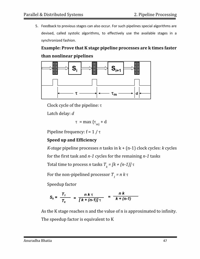
Example: Prove that K stage pipeline processes are k times faster
than nonlinear pipelines
Clock cycle of the pipeline:
Latch delay: d
= max {m}
+ d
Pipeline frequency: f = 1 /
Speed up and Efficiency
K-stage pipeline processes n tasks in k + (n-1) clock cycles: k cycles
for the first task and n-1 cycles for the remaining n-1 tasks
Total time to process n tasks Tk = [k + (n-1)]
For the non-pipelined processor T1 = n k
Speedup factor
As the K stage reaches n and the value of n is approximated to infinity.
The speedup factor is equivalent to K
Parallel & Distributed Systems 2. Pipeline Processing
Anuradha Bhatia 48
2.10 Pipeline control: scheduling
1. Controlling the sequence of tasks presented to a pipeline for execution is extremely
important for maximizing its utilization.
2. If two tasks are initiated requiring the same stage of the pipeline at the same time, a
collision occurs, which temporarily disrupts execution.
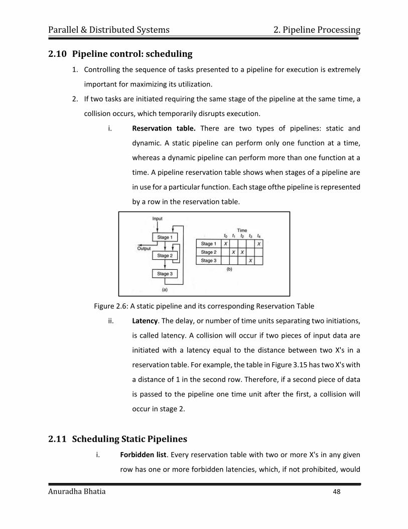
i. Reservation table. There are two types of pipelines: static and
dynamic. A static pipeline can perform only one function at a time,
whereas a dynamic pipeline can perform more than one function at a
time. A pipeline reservation table shows when stages of a pipeline are
in use for a particular function. Each stage ofthe pipeline is represented
by a row in the reservation table.
Figure 2.6: A static pipeline and its corresponding Reservation Table
ii. Latency. The delay, or number of time units separating two initiations,
is called latency. A collision will occur if two pieces of input data are
initiated with a latency equal to the distance between two X's in a
reservation table. For example, the table in Figure 3.15 has two X's with
a distance of 1 in the second row. Therefore, if a second piece of data
is passed to the pipeline one time unit after the first, a collision will
occur in stage 2.
2.11 Scheduling Static Pipelines
i. Forbidden list. Every reservation table with two or more X's in any given
row has one or more forbidden latencies, which, if not prohibited, would
Parallel & Distributed Systems 2. Pipeline Processing
Anuradha Bhatia 49
allow two data to collide or arrive at the same stage of the pipeline at the
same time. The forbidden list F is simply a list of integers corresponding to
these prohibited latencies.
ii. Collision vectors. A collision vector is a string of binary digits of length N+1,
where N is the largest forbidden latency in the forbidden list. The initial
collision vector, C, is created from the forbidden list in the following way:
each component ci of C, for i=0 to N, is 1 if i is an element of the forbidden
list. Otherwise, ci is zero. Zeros in the collision vector indicate allowable
latencies, or times when initiations are allowed into the pipeline.
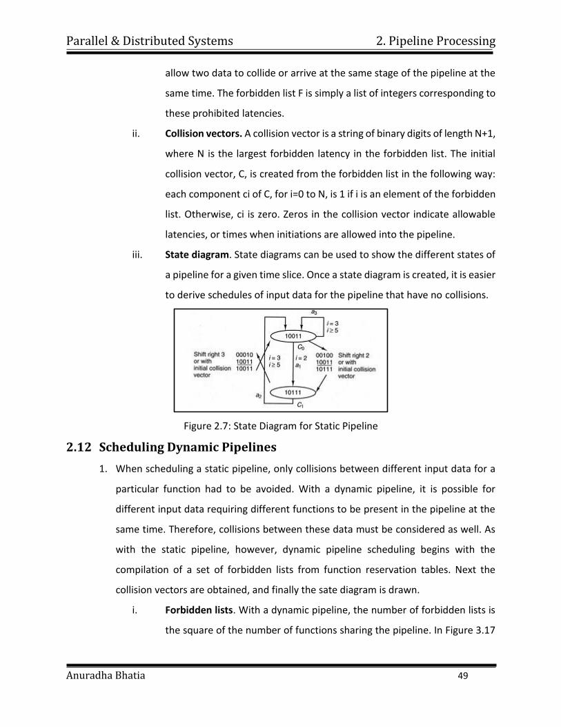
iii. State diagram. State diagrams can be used to show the different states of
a pipeline for a given time slice. Once a state diagram is created, it is easier
to derive schedules of input data for the pipeline that have no collisions.
Figure 2.7: State Diagram for Static Pipeline
2.12 Scheduling Dynamic Pipelines
1. When scheduling a static pipeline, only collisions between different input data for a
particular function had to be avoided. With a dynamic pipeline, it is possible for
different input data requiring different functions to be present in the pipeline at the
same time. Therefore, collisions between these data must be considered as well. As
with the static pipeline, however, dynamic pipeline scheduling begins with the
compilation of a set of forbidden lists from function reservation tables. Next the
collision vectors are obtained, and finally the sate diagram is drawn.
i. Forbidden lists. With a dynamic pipeline, the number of forbidden lists is
the square of the number of functions sharing the pipeline. In Figure 3.17
Parallel & Distributed Systems 2. Pipeline Processing
Anuradha Bhatia 50
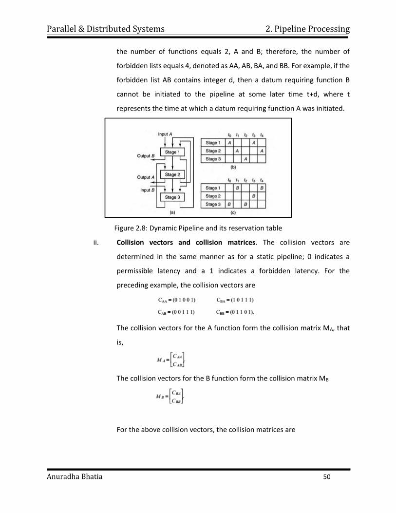
the number of functions equals 2, A and B; therefore, the number of
forbidden lists equals 4, denoted as AA, AB, BA, and BB. For example, if the
forbidden list AB contains integer d, then a datum requiring function B
cannot be initiated to the pipeline at some later time t+d, where t
represents the time at which a datum requiring function A was initiated.
Figure 2.8: Dynamic Pipeline and its reservation table
ii. Collision vectors and collision matrices. The collision vectors are
determined in the same manner as for a static pipeline; 0 indicates a
permissible latency and a 1 indicates a forbidden latency. For the
preceding example, the collision vectors are
The collision vectors for the A function form the collision matrix MA, that
is,
The collision vectors for the B function form the collision matrix MB
For the above collision vectors, the collision matrices are
Parallel & Distributed Systems 2. Pipeline Processing
Anuradha Bhatia 51
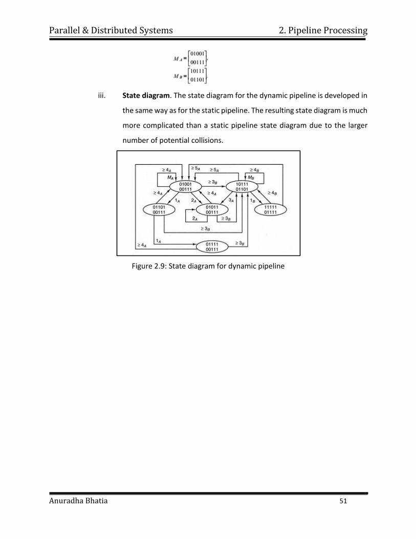
iii. State diagram. The state diagram for the dynamic pipeline is developed in
the same way as for the static pipeline. The resulting state diagram is much
more complicated than a static pipeline state diagram due to the larger
number of potential collisions.
Figure 2.9: State diagram for dynamic pipeline
Parallel & Distributed Systems
Anuradha Bhatia
3. Synchronous Parallel Processing
CONTENTS
3.1 Introduction, Example-SIMD Architecture and Programming Principles
3.2 SIMD Parallel Algorithms
3.3 Data Mapping and memory in array processors
3.4 Case studies of SIMD parallel Processors
Parallel & Distributed Systems 3. Synchronous Parallel Processing
Anuradha Bhatia 53
3.1 Principle of SIMD
1. The Synchronous parallel architectures coordinate Concurrent operations in
lockstep through global clocks, central control units, or vector unit controllers.
2. A synchronous array of parallel processors is called an array processor. These
processors are composed of N identical processing elements (PES) under the
supervision of a one control unit (CU) This Control unit is a computer with high
speed registers, local memory and arithmetic logic unit.
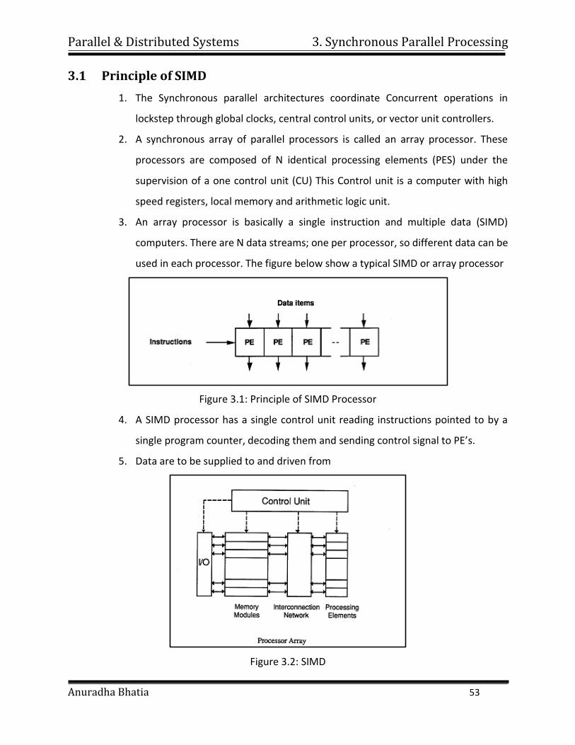
3. An array processor is basically a single instruction and multiple data (SIMD)
computers. There are N data streams; one per processor, so different data can be
used in each processor. The figure below show a typical SIMD or array processor
Figure 3.1: Principle of SIMD Processor
4. A SIMD processor has a single control unit reading instructions pointed to by a
single program counter, decoding them and sending control signal to PE’s.
5. Data are to be supplied to and driven from
Figure 3.2: SIMD
Parallel & Distributed Systems 3. Synchronous Parallel Processing
Anuradha Bhatia 54
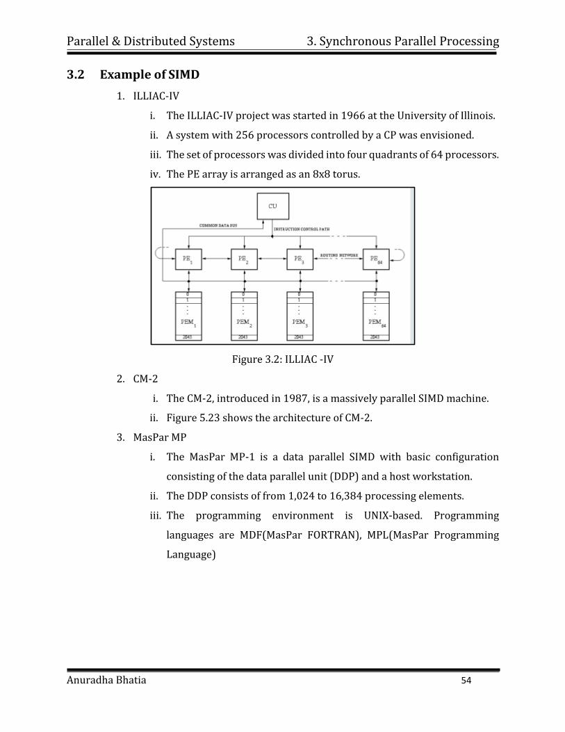
3.2 Example of SIMD
1. ILLIAC-IV
i. The ILLIAC-IV project was started in 1966 at the University of Illinois.
ii. A system with 256 processors controlled by a CP was envisioned.
iii. The set of processors was divided into four quadrants of 64 processors.
iv. The PE array is arranged as an 8x8 torus.
Figure 3.2: ILLIAC -IV
2. CM-2
i. The CM-2, introduced in 1987, is a massively parallel SIMD machine.
ii. Figure 5.23 shows the architecture of CM-2.
3. MasPar MP
i. The MasPar MP-1 is a data parallel SIMD with basic configuration
consisting of the data parallel unit (DDP) and a host workstation.
ii. The DDP consists of from 1,024 to 16,384 processing elements.
iii. The programming environment is UNIX-based. Programming
languages are MDF(MasPar FORTRAN), MPL(MasPar Programming
Language)
Parallel & Distributed Systems 3. Synchronous Parallel Processing
Anuradha Bhatia 55
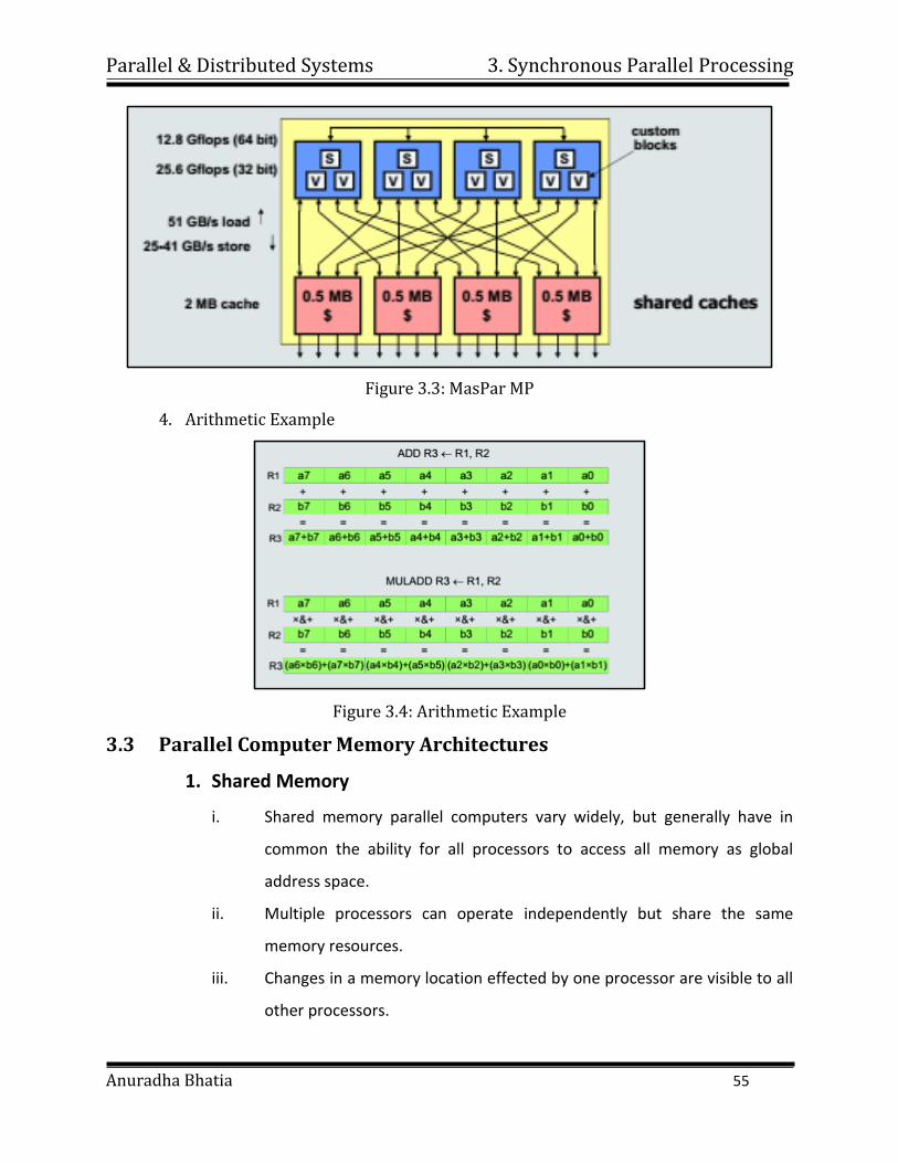
Figure 3.3: MasPar MP
4. Arithmetic Example
Figure 3.4: Arithmetic Example
3.3 Parallel Computer Memory Architectures
1. Shared Memory
i. Shared memory parallel computers vary widely, but generally have in
common the ability for all processors to access all memory as global
address space.
ii. Multiple processors can operate independently but share the same
memory resources.
iii. Changes in a memory location effected by one processor are visible to all
other processors.
Parallel & Distributed Systems 3. Synchronous Parallel Processing
Anuradha Bhatia 56
iv. Shared memory machines can be divided into two main classes based upon
memory access times: UMA and NUMA.
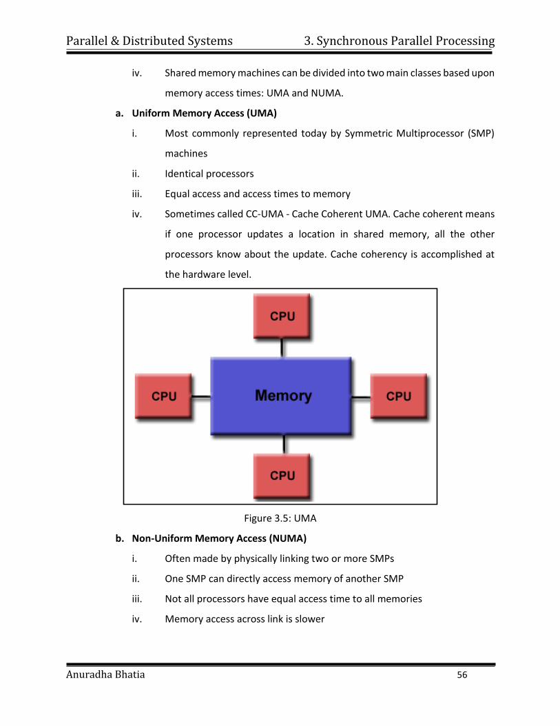
a. Uniform Memory Access (UMA)
i. Most commonly represented today by Symmetric Multiprocessor (SMP)
machines
ii. Identical processors
iii. Equal access and access times to memory
iv. Sometimes called CC-UMA - Cache Coherent UMA. Cache coherent means
if one processor updates a location in shared memory, all the other
processors know about the update. Cache coherency is accomplished at
the hardware level.
Figure 3.5: UMA
b. Non-Uniform Memory Access (NUMA)
i. Often made by physically linking two or more SMPs
ii. One SMP can directly access memory of another SMP
iii. Not all processors have equal access time to all memories
iv. Memory access across link is slower
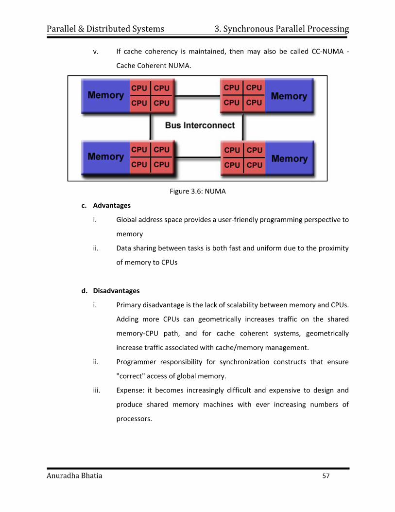
Parallel & Distributed Systems 3. Synchronous Parallel Processing
Anuradha Bhatia 57
v. If cache coherency is maintained, then may also be called CC-NUMA -
Cache Coherent NUMA.
Figure 3.6: NUMA
c. Advantages
i. Global address space provides a user-friendly programming perspective to
memory
ii. Data sharing between tasks is both fast and uniform due to the proximity
of memory to CPUs
d. Disadvantages
i. Primary disadvantage is the lack of scalability between memory and CPUs.
Adding more CPUs can geometrically increases traffic on the shared
memory-CPU path, and for cache coherent systems, geometrically
increase traffic associated with cache/memory management.
ii. Programmer responsibility for synchronization constructs that ensure
"correct" access of global memory.
iii. Expense: it becomes increasingly difficult and expensive to design and
produce shared memory machines with ever increasing numbers of
processors.
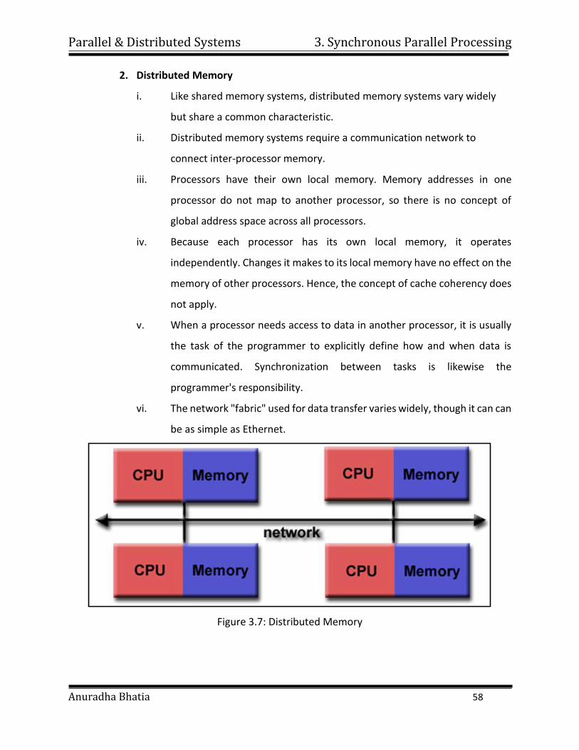
Parallel & Distributed Systems 3. Synchronous Parallel Processing
Anuradha Bhatia 58
2. Distributed Memory
i. Like shared memory systems, distributed memory systems vary widely
but share a common characteristic.
ii. Distributed memory systems require a communication network to
connect inter-processor memory.
iii. Processors have their own local memory. Memory addresses in one
processor do not map to another processor, so there is no concept of
global address space across all processors.
iv. Because each processor has its own local memory, it operates
independently. Changes it makes to its local memory have no effect on the
memory of other processors. Hence, the concept of cache coherency does
not apply.
v. When a processor needs access to data in another processor, it is usually
the task of the programmer to explicitly define how and when data is
communicated. Synchronization between tasks is likewise the
programmer's responsibility.
vi. The network "fabric" used for data transfer varies widely, though it can can
be as simple as Ethernet.
Figure 3.7: Distributed Memory
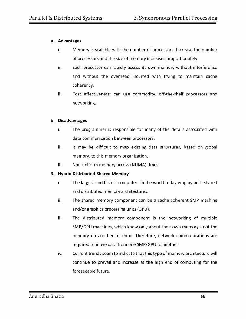
Parallel & Distributed Systems 3. Synchronous Parallel Processing
Anuradha Bhatia 59
a. Advantages
i. Memory is scalable with the number of processors. Increase the number
of processors and the size of memory increases proportionately.
ii. Each processor can rapidly access its own memory without interference
and without the overhead incurred with trying to maintain cache
coherency.
iii. Cost effectiveness: can use commodity, off-the-shelf processors and
networking.
b. Disadvantages
i. The programmer is responsible for many of the details associated with
data communication between processors.
ii. It may be difficult to map existing data structures, based on global
memory, to this memory organization.
iii. Non-uniform memory access (NUMA) times
3. Hybrid Distributed-Shared Memory
i. The largest and fastest computers in the world today employ both shared
and distributed memory architectures.
ii. The shared memory component can be a cache coherent SMP machine
and/or graphics processing units (GPU).
iii. The distributed memory component is the networking of multiple
SMP/GPU machines, which know only about their own memory - not the
memory on another machine. Therefore, network communications are
required to move data from one SMP/GPU to another.
iv. Current trends seem to indicate that this type of memory architecture will
continue to prevail and increase at the high end of computing for the
foreseeable future.
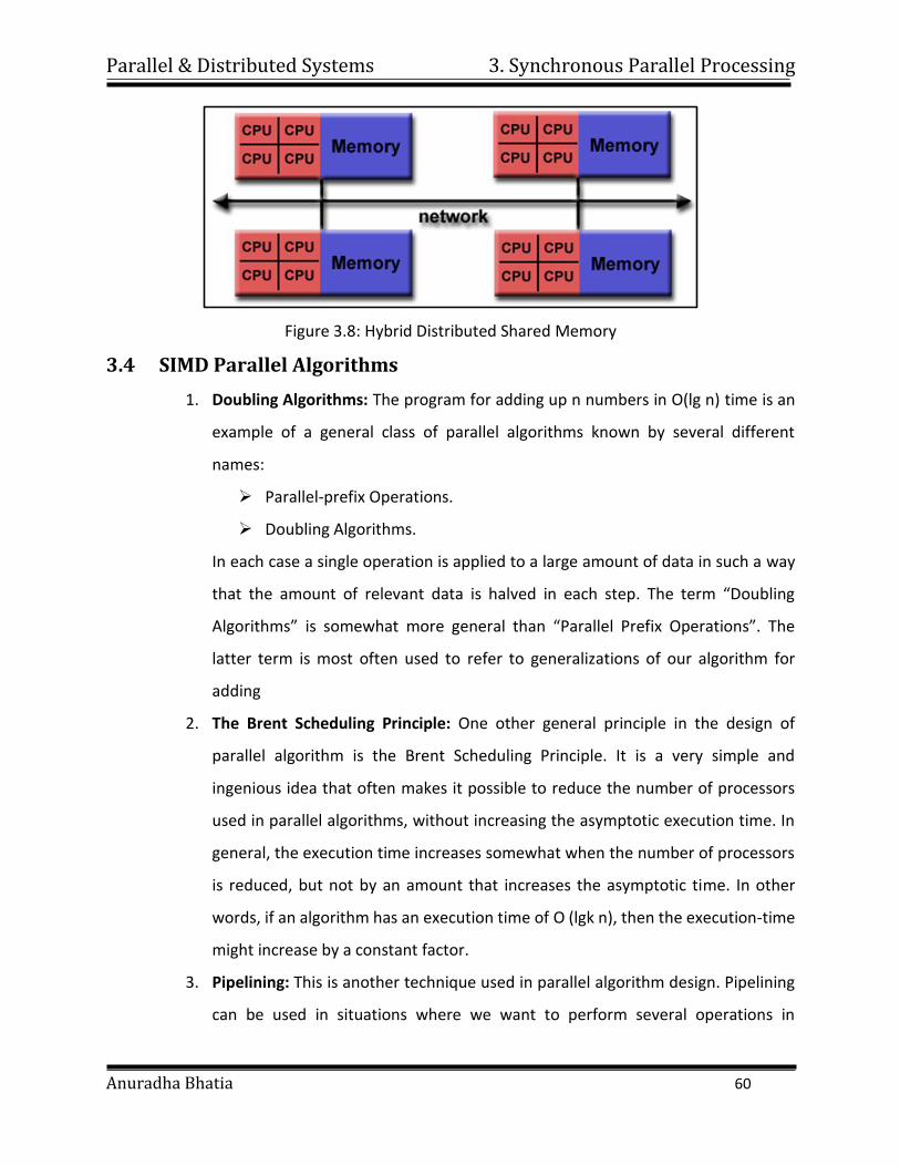
Parallel & Distributed Systems 3. Synchronous Parallel Processing
Anuradha Bhatia 60
Figure 3.8: Hybrid Distributed Shared Memory
3.4 SIMD Parallel Algorithms
1. Doubling Algorithms: The program for adding up n numbers in O(lg n) time is an
example of a general class of parallel algorithms known by several different
names:
Parallel-prefix Operations.
Doubling Algorithms.
In each case a single operation is applied to a large amount of data in such a way
that the amount of relevant data is halved in each step. The term “Doubling
Algorithms” is somewhat more general than “Parallel Prefix Operations”. The
latter term is most often used to refer to generalizations of our algorithm for
adding
2. The Brent Scheduling Principle: One other general principle in the design of
parallel algorithm is the Brent Scheduling Principle. It is a very simple and
ingenious idea that often makes it possible to reduce the number of processors
used in parallel algorithms, without increasing the asymptotic execution time. In
general, the execution time increases somewhat when the number of processors
is reduced, but not by an amount that increases the asymptotic time. In other
words, if an algorithm has an execution time of O (lgk n), then the execution-time
might increase by a constant factor.
3. Pipelining: This is another technique used in parallel algorithm design. Pipelining
can be used in situations where we want to perform several operations in
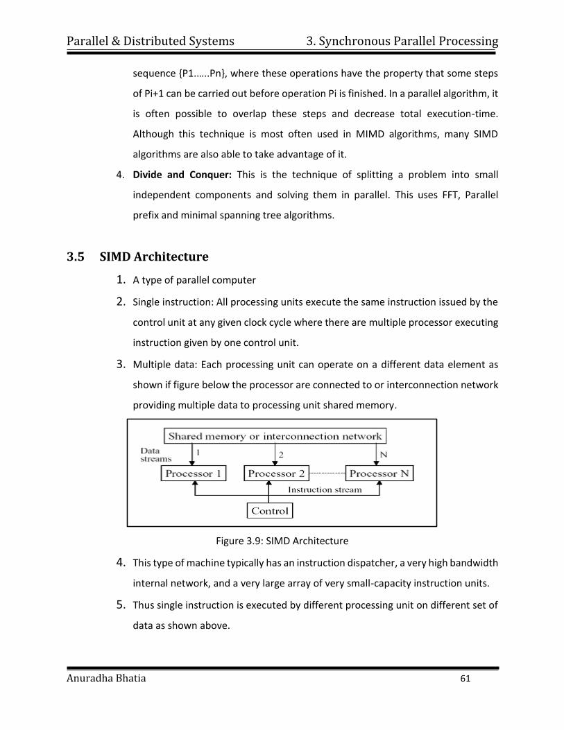
Parallel & Distributed Systems 3. Synchronous Parallel Processing
Anuradha Bhatia 61
sequence {P1.…..Pn}, where these operations have the property that some steps
of Pi+1 can be carried out before operation Pi is finished. In a parallel algorithm, it
is often possible to overlap these steps and decrease total execution-time.
Although this technique is most often used in MIMD algorithms, many SIMD
algorithms are also able to take advantage of it.
4. Divide and Conquer: This is the technique of splitting a problem into small
independent components and solving them in parallel. This uses FFT, Parallel
prefix and minimal spanning tree algorithms.
3.5 SIMD Architecture
1. A type of parallel computer
2. Single instruction: All processing units execute the same instruction issued by the
control unit at any given clock cycle where there are multiple processor executing
instruction given by one control unit.
3. Multiple data: Each processing unit can operate on a different data element as
shown if figure below the processor are connected to or interconnection network
providing multiple data to processing unit shared memory.
Figure 3.9: SIMD Architecture
4. This type of machine typically has an instruction dispatcher, a very high bandwidth
internal network, and a very large array of very small-capacity instruction units.
5. Thus single instruction is executed by different processing unit on different set of
data as shown above.
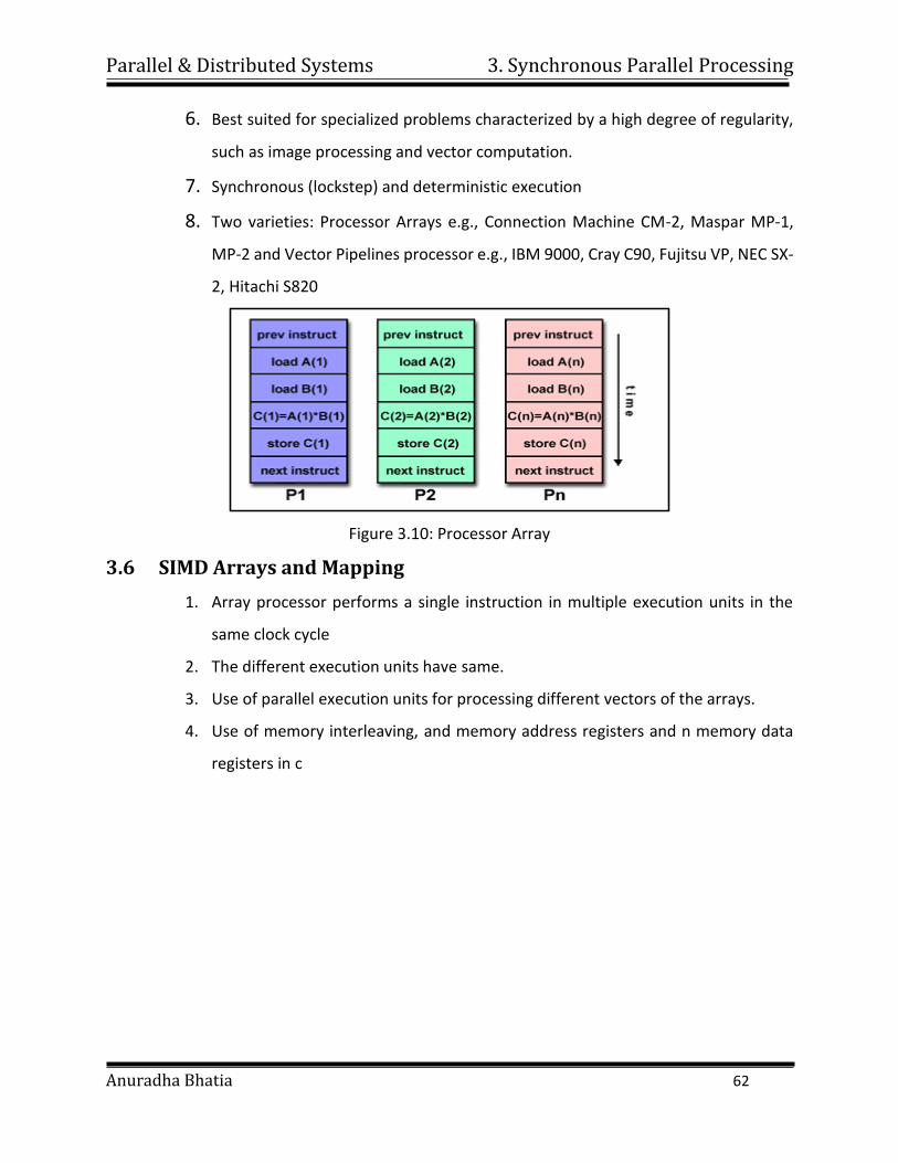
Parallel & Distributed Systems 3. Synchronous Parallel Processing
Anuradha Bhatia 62
6. Best suited for specialized problems characterized by a high degree of regularity,
such as image processing and vector computation.
7. Synchronous (lockstep) and deterministic execution
8. Two varieties: Processor Arrays e.g., Connection Machine CM-2, Maspar MP-1,
MP-2 and Vector Pipelines processor e.g., IBM 9000, Cray C90, Fujitsu VP, NEC SX-
2, Hitachi S820
Figure 3.10: Processor Array
3.6 SIMD Arrays and Mapping
1. Array processor performs a single instruction in multiple execution units in the
same clock cycle
2. The different execution units have same.
3. Use of parallel execution units for processing different vectors of the arrays.
4. Use of memory interleaving, and memory address registers and n memory data
registers in c
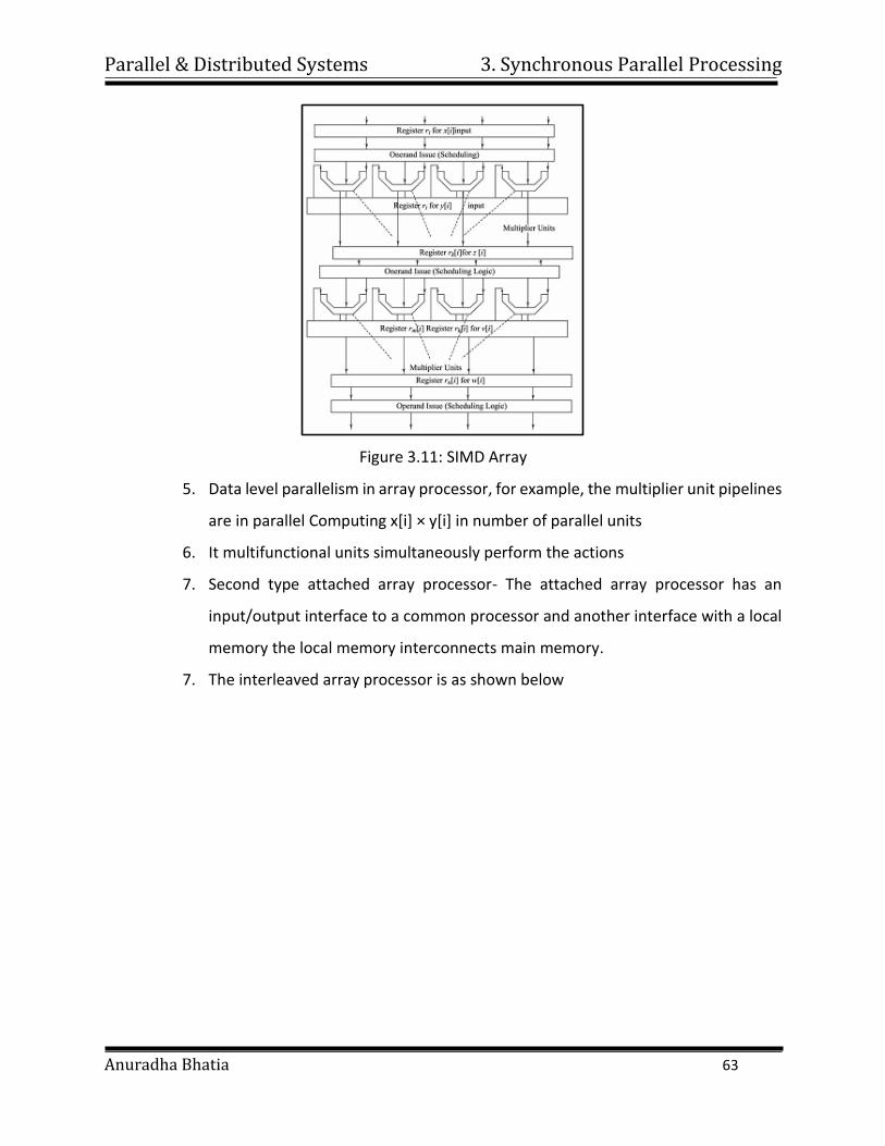
Parallel & Distributed Systems 3. Synchronous Parallel Processing
Anuradha Bhatia 63
Figure 3.11: SIMD Array
5. Data level parallelism in array processor, for example, the multiplier unit pipelines
are in parallel Computing x[i] × y[i] in number of parallel units
6. It multifunctional units simultaneously perform the actions
7. Second type attached array processor- The attached array processor has an
input/output interface to a common processor and another interface with a local
memory the local memory interconnects main memory.
7. The interleaved array processor is as shown below
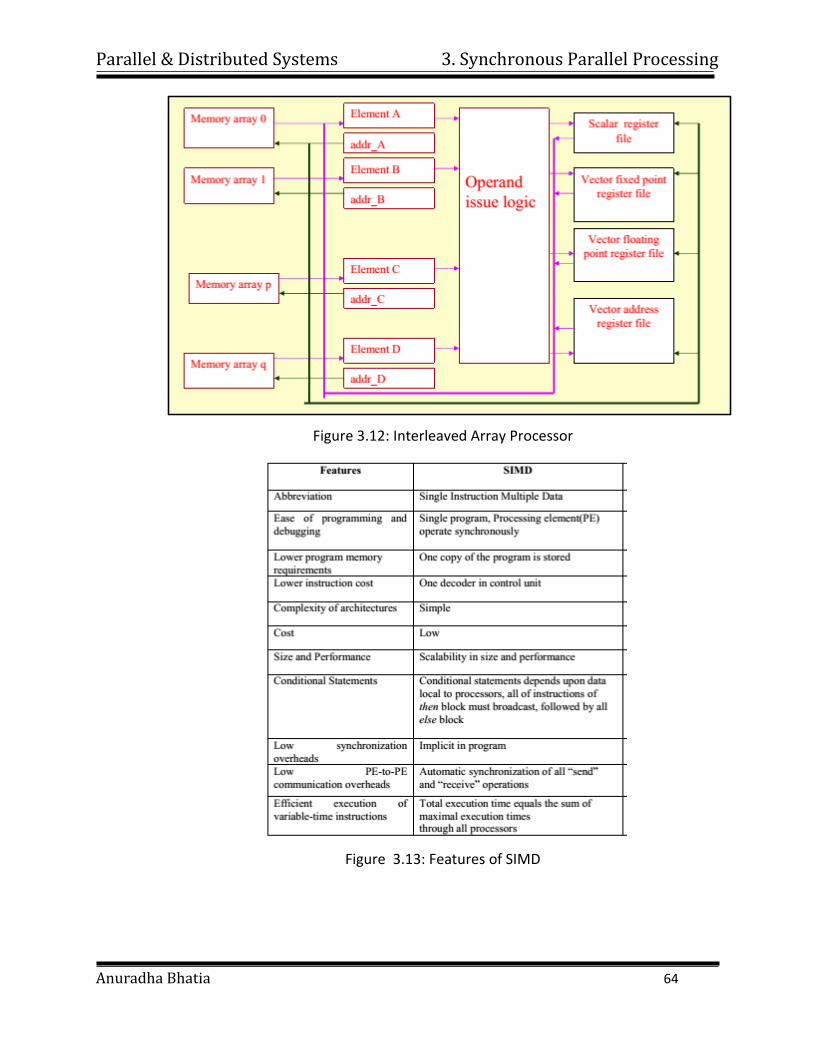
Parallel & Distributed Systems 3. Synchronous Parallel Processing
Anuradha Bhatia 64
Figure 3.12: Interleaved Array Processor
Figure 3.13: Features of SIMD
Parallel & Distributed Systems
Anuradha Bhatia
4. Introduction to Distributed Systems
CONTENTS
4.1 Definition
4.2 Issues, Goals
4.3 Types of distributed systems
4.4 Distributed System Models
4.5 Hardware concepts
4.6 Software Concept
4.7 Models of Middleware
4.8 Services offered by middleware
4.9 Client Server model.
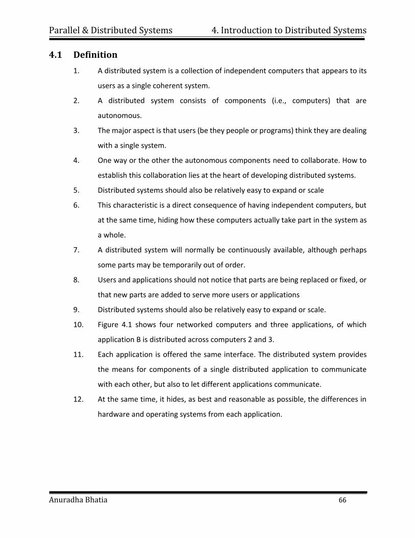
Parallel & Distributed Systems 4. Introduction to Distributed Systems
Anuradha Bhatia 66
4.1 Definition
1. A distributed system is a collection of independent computers that appears to its
users as a single coherent system.
2. A distributed system consists of components (i.e., computers) that are
autonomous.
3. The major aspect is that users (be they people or programs) think they are dealing
with a single system.
4. One way or the other the autonomous components need to collaborate. How to
establish this collaboration lies at the heart of developing distributed systems.
5. Distributed systems should also be relatively easy to expand or scale
6. This characteristic is a direct consequence of having independent computers, but
at the same time, hiding how these computers actually take part in the system as
a whole.
7. A distributed system will normally be continuously available, although perhaps
some parts may be temporarily out of order.
8. Users and applications should not notice that parts are being replaced or fixed, or
that new parts are added to serve more users or applications
9. Distributed systems should also be relatively easy to expand or scale.
10. Figure 4.1 shows four networked computers and three applications, of which
application B is distributed across computers 2 and 3.
11. Each application is offered the same interface. The distributed system provides
the means for components of a single distributed application to communicate
with each other, but also to let different applications communicate.
12. At the same time, it hides, as best and reasonable as possible, the differences in
hardware and operating systems from each application.
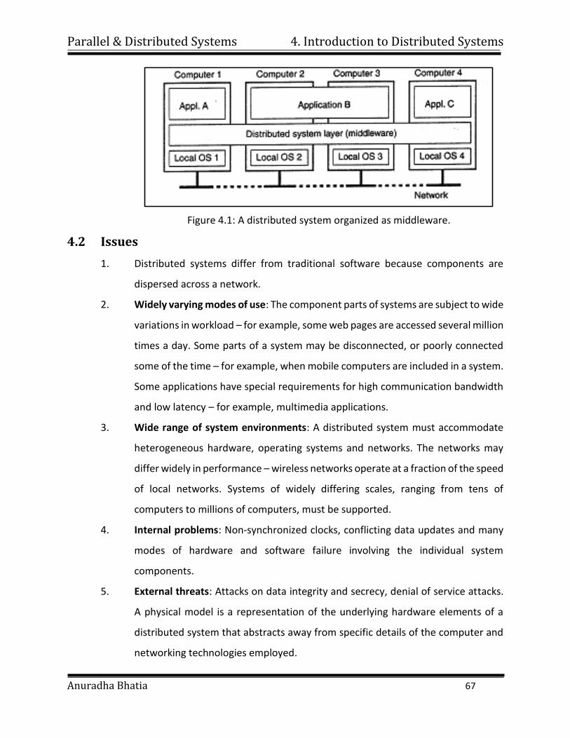
Parallel & Distributed Systems 4. Introduction to Distributed Systems
Anuradha Bhatia 67
Figure 4.1: A distributed system organized as middleware.
4.2 Issues
1. Distributed systems differ from traditional software because components are
dispersed across a network.
2. Widely varying modes of use: The component parts of systems are subject to wide
variations in workload – for example, some web pages are accessed several million
times a day. Some parts of a system may be disconnected, or poorly connected
some of the time – for example, when mobile computers are included in a system.
Some applications have special requirements for high communication bandwidth
and low latency – for example, multimedia applications.
3. Wide range of system environments: A distributed system must accommodate
heterogeneous hardware, operating systems and networks. The networks may
differ widely in performance – wireless networks operate at a fraction of the speed
of local networks. Systems of widely differing scales, ranging from tens of
computers to millions of computers, must be supported.
4. Internal problems: Non-synchronized clocks, conflicting data updates and many
modes of hardware and software failure involving the individual system
components.
5. External threats: Attacks on data integrity and secrecy, denial of service attacks.
A physical model is a representation of the underlying hardware elements of a
distributed system that abstracts away from specific details of the computer and
networking technologies employed.
Parallel & Distributed Systems 4. Introduction to Distributed Systems
Anuradha Bhatia 68
6. Not taking this dispersion into account during design time is what makes so many
systems needlessly complex and results in mistakes that need to be patched later
on. Peter Deutsch, then at Sun Microsystems, formulated these mistakes as the
following false assumptions that everyone makes when developing a distributed
application for the first time:
i. The network is reliable.
ii. The network is secure.
iii. The network is homogeneous.
iv. The topology does not change.
v. Latency is zero.
vi. Bandwidth is infinite.
vii. Transport cost is zero.
viii. There is one administrator.
4.3 Goals
1. Four important goals that should be met to make building a distributed system
worth the effort.
2. A distributed system should make resources easily accessible; it should reasonably
hide the fact that resources are distributed across a network; it should be open;
and it should be scalable.
i. Making Resources Accessible: The main goal of a distributed system is to
make it easy for the users (and applications) to access remote resources,
and to share them in a controlled and efficient way. Resources can be just
about anything, but typical examples include things like printers,
computers, storage facilities, data, files, Web pages, and networks, to
name just a few. There are many reasons for wanting to share resources.
One obvious reason is that of economics. For example, it is cheaper to let
a printer be shared by several users in a small office than having to buy and
maintain a separate printer for each user. Likewise, it makes economic
Parallel & Distributed Systems 4. Introduction to Distributed Systems
Anuradha Bhatia 69
sense to share costly resources such as supercomputers, high-
performance storage systems, image setters, and other expensive
peripherals. Connecting users and resources also makes it easier to
collaborate and exchange information, as is clearly illustrated by the
success of the Internet with its simple protocols for exchanging files, mail,
documents, audio, and video. The connectivity of the Internet is now
leading to numerous virtual organizations in which geographically widely-
dispersed groups of people work together by means of groupware, that is,
software for collaborative editing, teleconferencing, and so on. Likewise,
the Internet connectivity has enabled electronic commerce allowing us to
buy and sell all kinds of goods without actually having to go to a store or
even leave home.
ii. Distribution Transparency: An important goal of a distributed system is to
hide the fact that its processes and resources are physically distributed
across multiple computers. A distributed system that is able to present
itself to users and applications as if it were only a single computer system
is said to be transparent. Let us first take a look at what kinds of
transparency exist in distributed systems. After that we will address the
more general question whether transparency is always required. Access
transparency deals with hiding differences in data representation and the
way that resources can be accessed by users. At a basic level, we wish to
hide differences in machine architectures, but more important is that we
reach agreement on how data is to be represented by different machines
and operating systems. For example, a distributed system may have
computer systems that run different operating systems, each having their
own file-naming conventions. Differences in naming conventions, as well
as how files can be manipulated, should all be hidden from users and
applications. Another example is where we need to guarantee that several
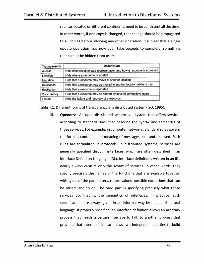
Parallel & Distributed Systems 4. Introduction to Distributed Systems
Anuradha Bhatia 70
replicas, located on different continents, need to be consistent all the time.
In other words, if one copy is changed, that change should be propagated
to all copies before allowing any other operation. It is clear that a single
update operation may now even take seconds to complete, something
that cannot be hidden from users.
Table 4.1: Different forms of transparency in a distributed system (ISO, 1995).
iii. Openness: An open distributed system is a system that offers services
according to standard rules that describe the syntax and semantics of
those services. For example, in computer networks, standard rules govern
the format, contents, and meaning of messages sent and received. Such
rules are formalized in protocols. In distributed systems, services are
generally specified through interfaces, which are often described in an
Interface Definition Language (IDL). Interface definitions written in an IDL
nearly always capture only the syntax of services. In other words, they
specify precisely the names of the functions that are available together
with types of the parameters, return values, possible exceptions that can
be raised, and so on. The hard part is specifying precisely what those
services do, that is, the semantics of interfaces. In practice, such
specifications are always given in an informal way by means of natural
language. If properly specified, an interface definition allows an arbitrary
process that needs a certain interface to talk to another process that
provides that interface. It also allows two independent parties to build
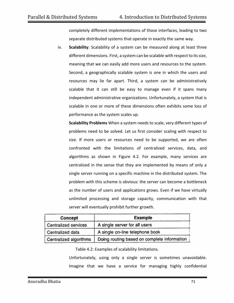
Parallel & Distributed Systems 4. Introduction to Distributed Systems
Anuradha Bhatia 71
completely different implementations of those interfaces, leading to two
separate distributed systems that operate in exactly the same way.
iv. Scalability: Scalability of a system can be measured along at least three
different dimensions. First, a system can be scalable with respect to its size,
meaning that we can easily add more users and resources to the system.
Second, a geographically scalable system is one in which the users and
resources may lie far apart. Third, a system can be administratively
scalable that it can still be easy to manage even if it spans many
independent administrative organizations. Unfortunately, a system that is
scalable in one or more of these dimensions often exhibits some loss of
performance as the system scales up.
Scalability Problems When a system needs to scale, very different types of
problems need to be solved. Let us first consider scaling with respect to
size. If more users or resources need to be supported, we are often
confronted with the limitations of centralized services, data, and
algorithms as shown in Figure 4.2. For example, many services are
centralized in the sense that they are implemented by means of only a
single server running on a specific machine in the distributed system. The
problem with this scheme is obvious: the server can become a bottleneck
as the number of users and applications grows. Even if we have virtually
unlimited processing and storage capacity, communication with that
server will eventually prohibit further growth.
Table 4.2: Examples of scalability limitations.
Unfortunately, using only a single server is sometimes unavoidable.
Imagine that we have a service for managing highly confidential
Parallel & Distributed Systems 4. Introduction to Distributed Systems
Anuradha Bhatia 72
information such as medical records, bank accounts and so on. In such
cases, it may be best to implement that service by means of a single server
in a highly secured separate room, and protected from other parts of the
distributed system through special network components. Copying the
server to several locations to enhance performance maybe out of the
question as it would make the service less secure. Finally, centralized
algorithms are also a bad idea. In a large distributed system, an enormous
number of messages have to be routed over many lines. From a theoretical
point of view, the optimal way to do this is collect complete information
about the load on all machines and lines, and then run an algorithm to
compute all the optimal routes. This information can then be spread
around the system to improve the routing. These algorithms generally
have the following characteristics, which distinguish them from centralized
algorithms:
1. No machine has complete information about the system state.
2. Machines make decisions based only on local information,
3. Failure of one machine does not ruin the algorithm.
4. There is no implicit assumption that a global clock exists.
Scaling Techniques Hiding communication latencies is important to
achieve geographical scalability. The basic idea is simple: try to avoid
waiting for responses to remote (and potentially distant) service requests
as much as possible. For example, when a service has been requested at a
remote machine, an alternative to waiting for a reply from the server is to
do other useful work at the requester's side. Essentially, what this means
is constructing the requesting application in such a way that it uses only
asynchronous communication. When a reply comes in, the application is
interrupted and a special handler is called to complete the previously-
issued request. Asynchronous communication can often be used in batch-
processing systems and parallel applications, in which more or less
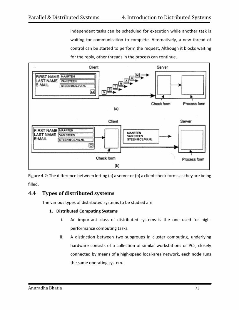
Parallel & Distributed Systems 4. Introduction to Distributed Systems
Anuradha Bhatia 73
independent tasks can be scheduled for execution while another task is
waiting for communication to complete. Alternatively, a new thread of
control can be started to perform the request. Although it blocks waiting
for the reply, other threads in the process can continue.
Figure 4.2: The difference between letting (a) a server or (b) a client check forms as they are being
filled.
4.4 Types of distributed systems
The various types of distributed systems to be studied are
1. Distributed Computing Systems
i. An important class of distributed systems is the one used for high-
performance computing tasks.
ii. A distinction between two subgroups in cluster computing, underlying
hardware consists of a collection of similar workstations or PCs, closely
connected by means of a high-speed local-area network, each node runs
the same operating system.
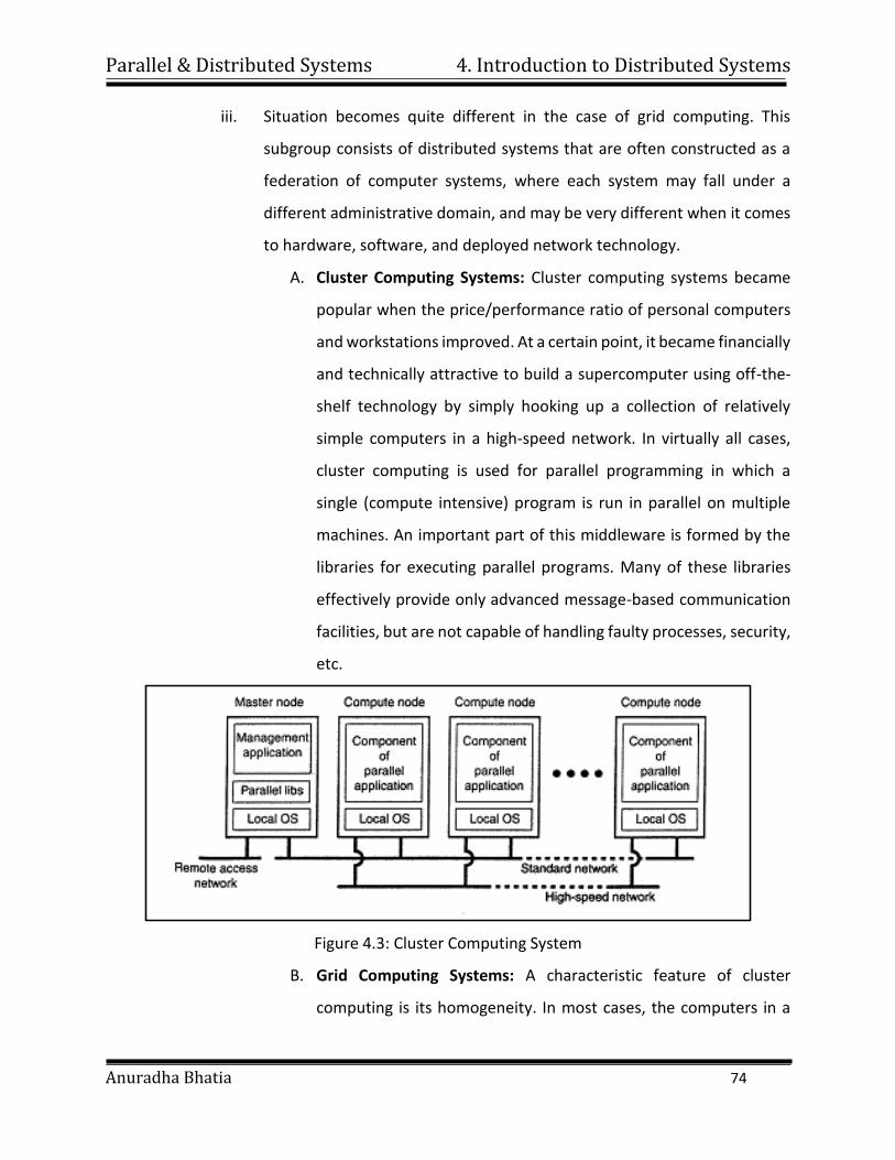
Parallel & Distributed Systems 4. Introduction to Distributed Systems
Anuradha Bhatia 74
iii. Situation becomes quite different in the case of grid computing. This
subgroup consists of distributed systems that are often constructed as a
federation of computer systems, where each system may fall under a
different administrative domain, and may be very different when it comes
to hardware, software, and deployed network technology.
A. Cluster Computing Systems: Cluster computing systems became
popular when the price/performance ratio of personal computers
and workstations improved. At a certain point, it became financially
and technically attractive to build a supercomputer using off-the-
shelf technology by simply hooking up a collection of relatively
simple computers in a high-speed network. In virtually all cases,
cluster computing is used for parallel programming in which a
single (compute intensive) program is run in parallel on multiple
machines. An important part of this middleware is formed by the
libraries for executing parallel programs. Many of these libraries
effectively provide only advanced message-based communication
facilities, but are not capable of handling faulty processes, security,
etc.
Figure 4.3: Cluster Computing System
B. Grid Computing Systems: A characteristic feature of cluster
computing is its homogeneity. In most cases, the computers in a
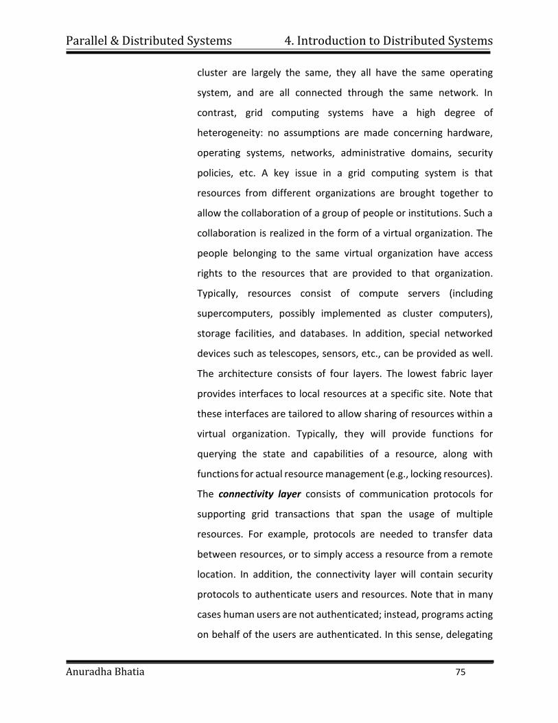
Parallel & Distributed Systems 4. Introduction to Distributed Systems
Anuradha Bhatia 75
cluster are largely the same, they all have the same operating
system, and are all connected through the same network. In
contrast, grid computing systems have a high degree of
heterogeneity: no assumptions are made concerning hardware,
operating systems, networks, administrative domains, security
policies, etc. A key issue in a grid computing system is that
resources from different organizations are brought together to
allow the collaboration of a group of people or institutions. Such a
collaboration is realized in the form of a virtual organization. The
people belonging to the same virtual organization have access
rights to the resources that are provided to that organization.
Typically, resources consist of compute servers (including
supercomputers, possibly implemented as cluster computers),
storage facilities, and databases. In addition, special networked
devices such as telescopes, sensors, etc., can be provided as well.
The architecture consists of four layers. The lowest fabric layer
provides interfaces to local resources at a specific site. Note that
these interfaces are tailored to allow sharing of resources within a
virtual organization. Typically, they will provide functions for
querying the state and capabilities of a resource, along with
functions for actual resource management (e.g., locking resources).
The connectivity layer consists of communication protocols for
supporting grid transactions that span the usage of multiple
resources. For example, protocols are needed to transfer data
between resources, or to simply access a resource from a remote
location. In addition, the connectivity layer will contain security
protocols to authenticate users and resources. Note that in many
cases human users are not authenticated; instead, programs acting
on behalf of the users are authenticated. In this sense, delegating
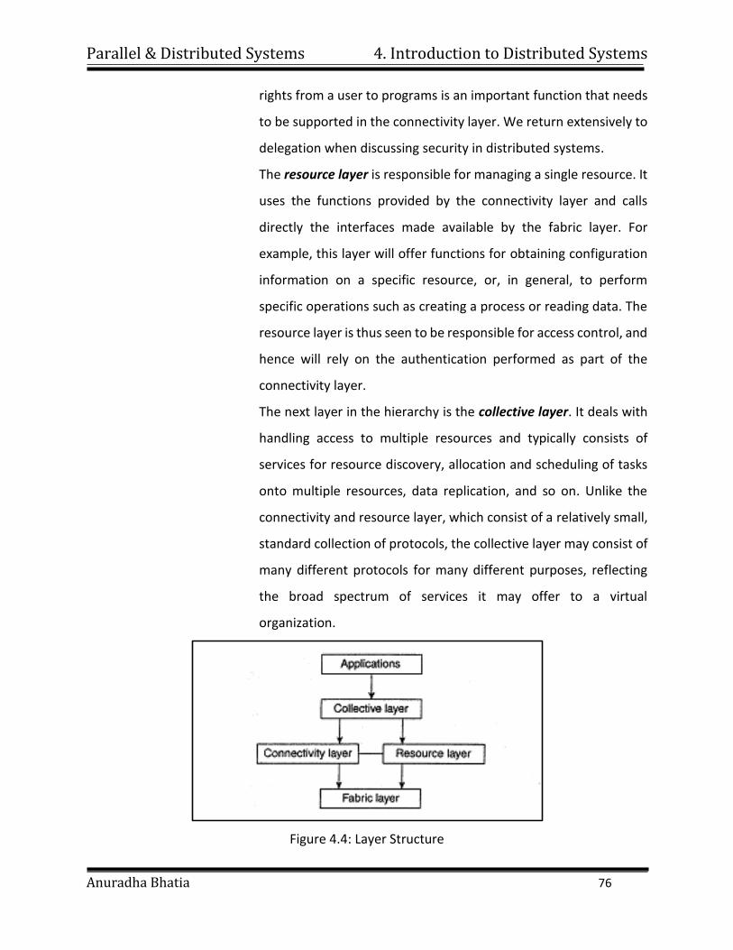
Parallel & Distributed Systems 4. Introduction to Distributed Systems
Anuradha Bhatia 76
rights from a user to programs is an important function that needs
to be supported in the connectivity layer. We return extensively to
delegation when discussing security in distributed systems.
The resource layer is responsible for managing a single resource. It
uses the functions provided by the connectivity layer and calls
directly the interfaces made available by the fabric layer. For
example, this layer will offer functions for obtaining configuration
information on a specific resource, or, in general, to perform
specific operations such as creating a process or reading data. The
resource layer is thus seen to be responsible for access control, and
hence will rely on the authentication performed as part of the
connectivity layer.
The next layer in the hierarchy is the collective layer. It deals with
handling access to multiple resources and typically consists of
services for resource discovery, allocation and scheduling of tasks
onto multiple resources, data replication, and so on. Unlike the
connectivity and resource layer, which consist of a relatively small,
standard collection of protocols, the collective layer may consist of
many different protocols for many different purposes, reflecting
the broad spectrum of services it may offer to a virtual
organization.
Figure 4.4: Layer Structure
Parallel & Distributed Systems 4. Introduction to Distributed Systems
Anuradha Bhatia 77
2. Distributed information Systems
Another important class of distributed systems is found in organizations that were
confronted with a wealth of networked applications, but for which
interoperability turned out to be a painful experience. Many of the existing
middleware solutions are the result of working with an infrastructure in which it
was easier to integrate applications into an enterprise-wide information system.
As applications became more sophisticated and were gradually separated into
independent components, it became clear that integration should also take place
by letting applications communicate directly with each other.
A. Transaction Processing Systems: practice, operations on a
database are usually carried out in the form of transactions.
Programming using transactions requires special primitives that
must either be supplied by the underlying distributed system or by
the language runtime system. Typical examples of transaction
primitives. The exact list of primitives depends on what kinds of
objects are being used in the transaction. Typical examples of
transaction primitives are shown in Table 4.3.
Table 4.1: Primitive and description
The exact list of primitives depends on what kinds of objects are
being used in the transaction (Gray and Reuter, 1993). In a mail
system, there might be primitives to send, receive, and forward
mail. In an accounting system, they might be quite different. READ
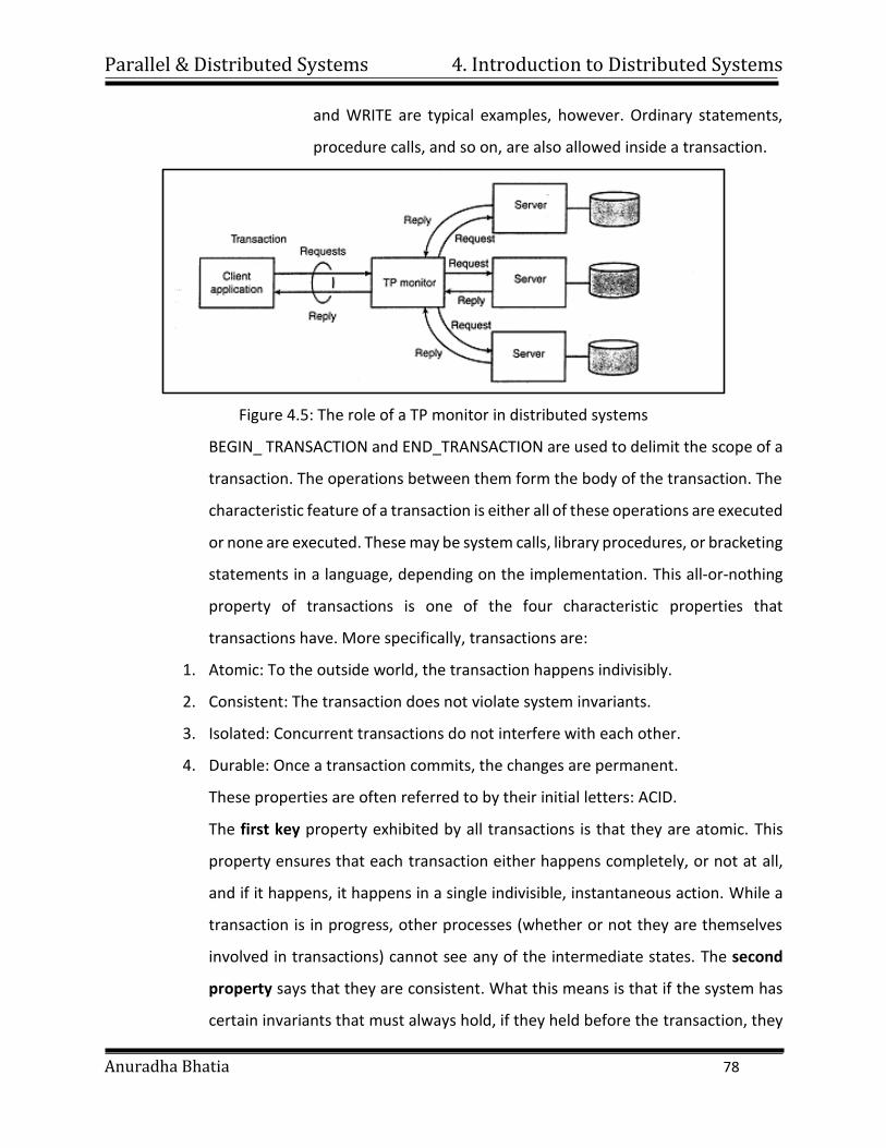
Parallel & Distributed Systems 4. Introduction to Distributed Systems
Anuradha Bhatia 78
and WRITE are typical examples, however. Ordinary statements,
procedure calls, and so on, are also allowed inside a transaction.
Figure 4.5: The role of a TP monitor in distributed systems
BEGIN_ TRANSACTION and END_TRANSACTION are used to delimit the scope of a
transaction. The operations between them form the body of the transaction. The
characteristic feature of a transaction is either all of these operations are executed
or none are executed. These may be system calls, library procedures, or bracketing
statements in a language, depending on the implementation. This all-or-nothing
property of transactions is one of the four characteristic properties that
transactions have. More specifically, transactions are:
1. Atomic: To the outside world, the transaction happens indivisibly.
2. Consistent: The transaction does not violate system invariants.
3. Isolated: Concurrent transactions do not interfere with each other.
4. Durable: Once a transaction commits, the changes are permanent.
These properties are often referred to by their initial letters: ACID.
The first key property exhibited by all transactions is that they are atomic. This
property ensures that each transaction either happens completely, or not at all,
and if it happens, it happens in a single indivisible, instantaneous action. While a
transaction is in progress, other processes (whether or not they are themselves
involved in transactions) cannot see any of the intermediate states. The second
property says that they are consistent. What this means is that if the system has
certain invariants that must always hold, if they held before the transaction, they
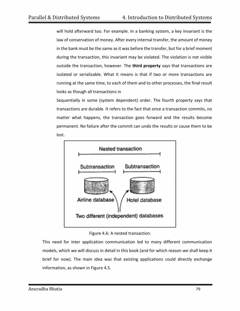
Parallel & Distributed Systems 4. Introduction to Distributed Systems
Anuradha Bhatia 79
will hold afterward too. For example. In a banking system, a key invariant is the
law of conservation of money. After every internal transfer, the amount of money
in the bank must be the same as it was before the transfer, but for a brief moment
during the transaction, this invariant may be violated. The violation is not visible
outside the transaction, however. The third property says that transactions are
isolated or serializable. What it means is that if two or more transactions are
running at the same time, to each of them and to other processes, the final result
looks as though all transactions in
Sequentially in some (system dependent) order. The fourth property says that
transactions are durable. It refers to the fact that once a transaction commits, no
matter what happens, the transaction goes forward and the results become
permanent. No failure after the commit can undo the results or cause them to be
lost.
Figure 4.6: A nested transaction.
This need for inter application communication led to many different communication
models, which we will discuss in detail in this book (and for which reason we shall keep it
brief for now). The main idea was that existing applications could directly exchange
information, as shown in Figure 4.5.
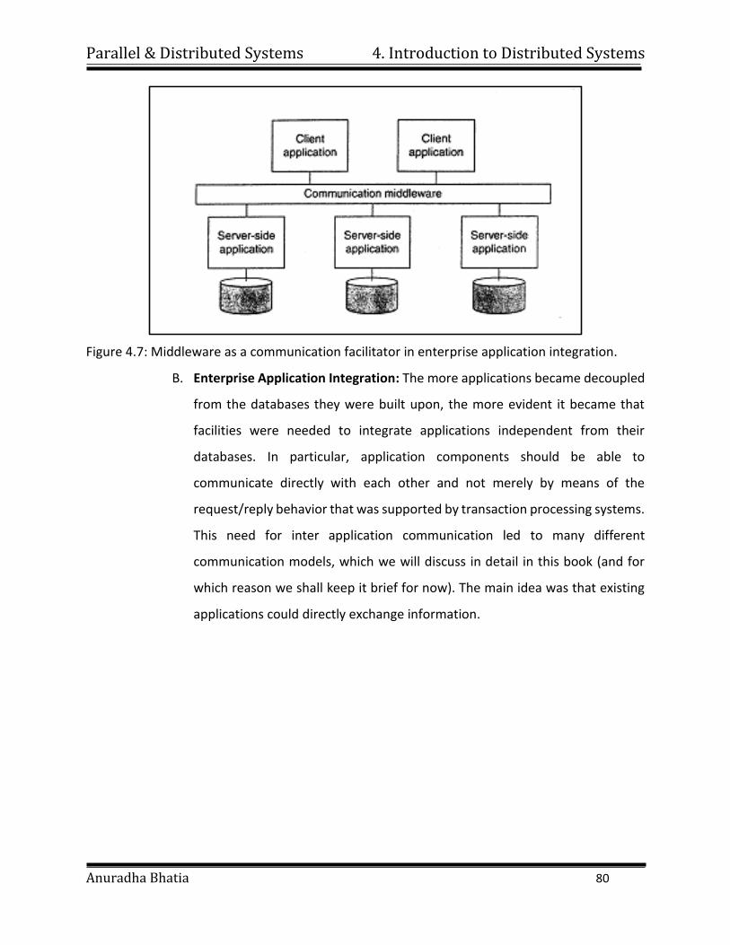
Parallel & Distributed Systems 4. Introduction to Distributed Systems
Anuradha Bhatia 80
Figure 4.7: Middleware as a communication facilitator in enterprise application integration.
B. Enterprise Application Integration: The more applications became decoupled
from the databases they were built upon, the more evident it became that
facilities were needed to integrate applications independent from their
databases. In particular, application components should be able to
communicate directly with each other and not merely by means of the
request/reply behavior that was supported by transaction processing systems.
This need for inter application communication led to many different
communication models, which we will discuss in detail in this book (and for
which reason we shall keep it brief for now). The main idea was that existing
applications could directly exchange information.
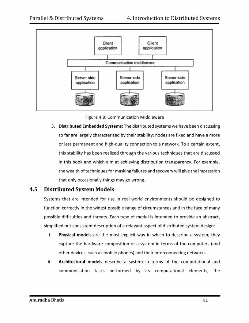
Parallel & Distributed Systems 4. Introduction to Distributed Systems
Anuradha Bhatia 81
Figure 4.8: Communication Middleware
3. Distributed Embedded Systems: The distributed systems we have been discussing
so far are largely characterized by their stability: nodes are fixed and have a more
or less permanent and high-quality connection to a network. To a certain extent,
this stability has been realized through the various techniques that are discussed
in this book and which aim at achieving distribution transparency. For example,
the wealth of techniques for masking failures and recovery will give the impression
that only occasionally things may go wrong.
4.5 Distributed System Models
Systems that are intended for use in real-world environments should be designed to
function correctly in the widest possible range of circumstances and in the face of many
possible difficulties and threats. Each type of model is intended to provide an abstract,
simplified but consistent description of a relevant aspect of distributed system design:
i. Physical models are the most explicit way in which to describe a system; they
capture the hardware composition of a system in terms of the computers (and
other devices, such as mobile phones) and their interconnecting networks.
ii. Architectural models describe a system in terms of the computational and
communication tasks performed by its computational elements; the
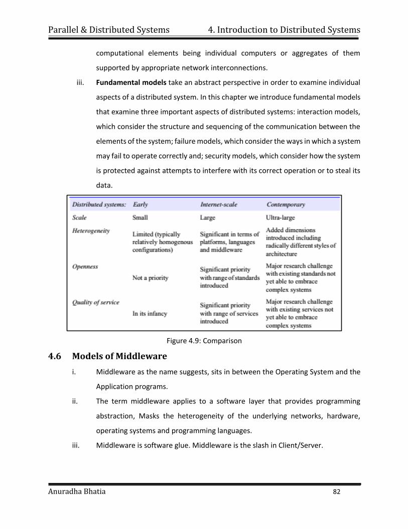
Parallel & Distributed Systems 4. Introduction to Distributed Systems
Anuradha Bhatia 82
computational elements being individual computers or aggregates of them
supported by appropriate network interconnections.
iii. Fundamental models take an abstract perspective in order to examine individual
aspects of a distributed system. In this chapter we introduce fundamental models
that examine three important aspects of distributed systems: interaction models,
which consider the structure and sequencing of the communication between the
elements of the system; failure models, which consider the ways in which a system
may fail to operate correctly and; security models, which consider how the system
is protected against attempts to interfere with its correct operation or to steal its
data.
Figure 4.9: Comparison
4.6 Models of Middleware
i. Middleware as the name suggests, sits in between the Operating System and the
Application programs.
ii. The term middleware applies to a software layer that provides programming
abstraction, Masks the heterogeneity of the underlying networks, hardware,
operating systems and programming languages.
iii. Middleware is software glue. Middleware is the slash in Client/Server.
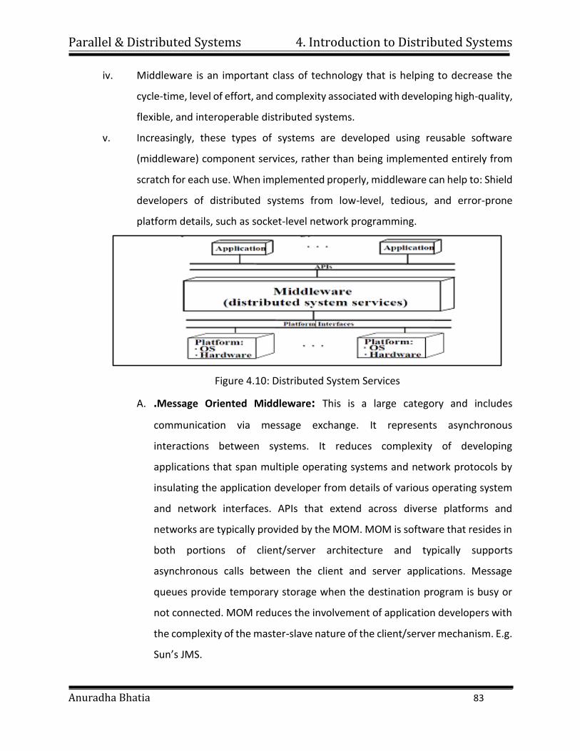
Parallel & Distributed Systems 4. Introduction to Distributed Systems
Anuradha Bhatia 83
iv. Middleware is an important class of technology that is helping to decrease the
cycle-time, level of effort, and complexity associated with developing high-quality,
flexible, and interoperable distributed systems.
v. Increasingly, these types of systems are developed using reusable software
(middleware) component services, rather than being implemented entirely from
scratch for each use. When implemented properly, middleware can help to: Shield
developers of distributed systems from low-level, tedious, and error-prone
platform details, such as socket-level network programming.
Figure 4.10: Distributed System Services
A. .Message Oriented Middleware: This is a large category and includes
communication via message exchange. It represents asynchronous
interactions between systems. It reduces complexity of developing
applications that span multiple operating systems and network protocols by
insulating the application developer from details of various operating system
and network interfaces. APIs that extend across diverse platforms and
networks are typically provided by the MOM. MOM is software that resides in
both portions of client/server architecture and typically supports
asynchronous calls between the client and server applications. Message
queues provide temporary storage when the destination program is busy or
not connected. MOM reduces the involvement of application developers with
the complexity of the master-slave nature of the client/server mechanism. E.g.
Sun’s JMS.
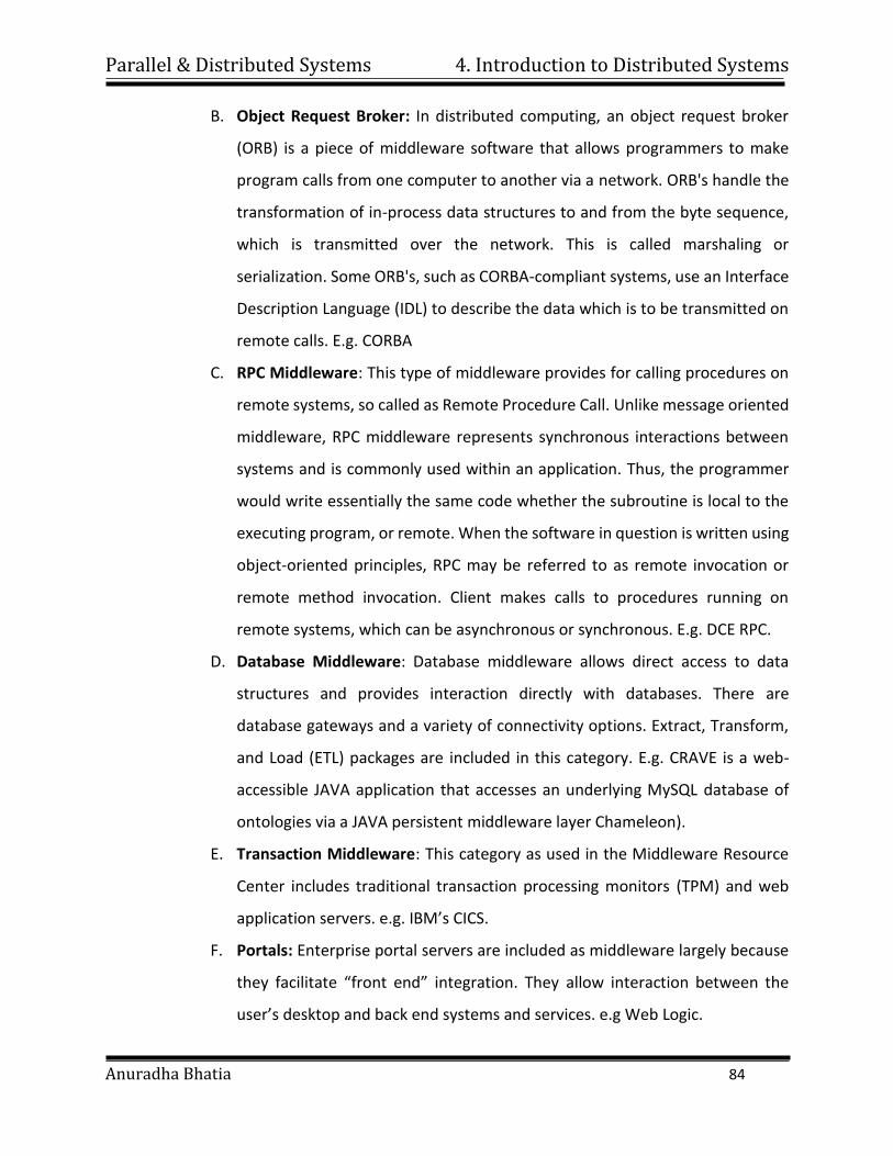
Parallel & Distributed Systems 4. Introduction to Distributed Systems
Anuradha Bhatia 84
B. Object Request Broker: In distributed computing, an object request broker
(ORB) is a piece of middleware software that allows programmers to make
program calls from one computer to another via a network. ORB's handle the
transformation of in-process data structures to and from the byte sequence,
which is transmitted over the network. This is called marshaling or
serialization. Some ORB's, such as CORBA-compliant systems, use an Interface
Description Language (IDL) to describe the data which is to be transmitted on
remote calls. E.g. CORBA
C. RPC Middleware: This type of middleware provides for calling procedures on
remote systems, so called as Remote Procedure Call. Unlike message oriented
middleware, RPC middleware represents synchronous interactions between
systems and is commonly used within an application. Thus, the programmer
would write essentially the same code whether the subroutine is local to the
executing program, or remote. When the software in question is written using
object-oriented principles, RPC may be referred to as remote invocation or
remote method invocation. Client makes calls to procedures running on
remote systems, which can be asynchronous or synchronous. E.g. DCE RPC.
D. Database Middleware: Database middleware allows direct access to data
structures and provides interaction directly with databases. There are
database gateways and a variety of connectivity options. Extract, Transform,
and Load (ETL) packages are included in this category. E.g. CRAVE is a web-
accessible JAVA application that accesses an underlying MySQL database of
ontologies via a JAVA persistent middleware layer Chameleon).
E. Transaction Middleware: This category as used in the Middleware Resource
Center includes traditional transaction processing monitors (TPM) and web
application servers. e.g. IBM’s CICS.
F. Portals: Enterprise portal servers are included as middleware largely because
they facilitate “front end” integration. They allow interaction between the
user’s desktop and back end systems and services. e.g Web Logic.
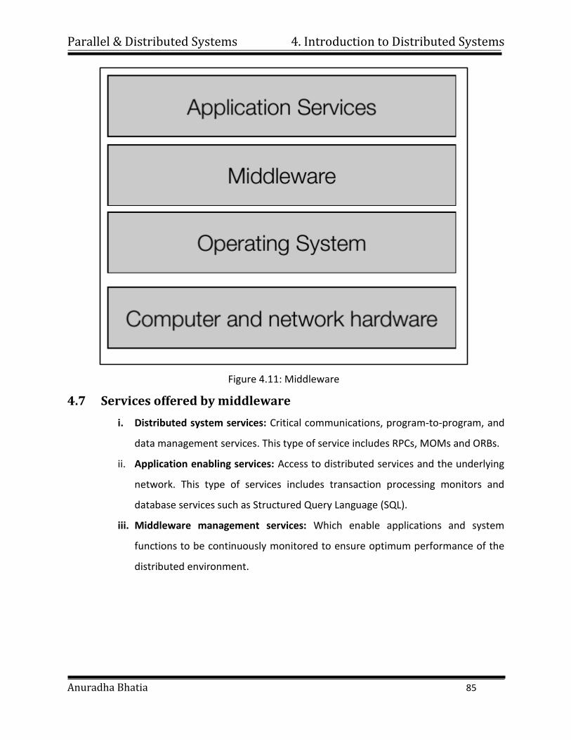
Parallel & Distributed Systems 4. Introduction to Distributed Systems
Anuradha Bhatia 85
Figure 4.11: Middleware
4.7 Services offered by middleware
i. Distributed system services: Critical communications, program-to-program, and
data management services. This type of service includes RPCs, MOMs and ORBs.
ii. Application enabling services: Access to distributed services and the underlying
network. This type of services includes transaction processing monitors and
database services such as Structured Query Language (SQL).
iii. Middleware management services: Which enable applications and system
functions to be continuously monitored to ensure optimum performance of the
distributed environment.
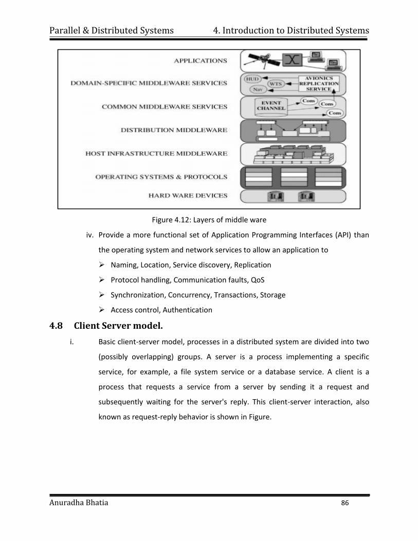
Parallel & Distributed Systems 4. Introduction to Distributed Systems
Anuradha Bhatia 86
Figure 4.12: Layers of middle ware
iv. Provide a more functional set of Application Programming Interfaces (API) than
the operating system and network services to allow an application to
Naming, Location, Service discovery, Replication
Protocol handling, Communication faults, QoS
Synchronization, Concurrency, Transactions, Storage
Access control, Authentication
4.8 Client Server model.
i. Basic client-server model, processes in a distributed system are divided into two
(possibly overlapping) groups. A server is a process implementing a specific
service, for example, a file system service or a database service. A client is a
process that requests a service from a server by sending it a request and
subsequently waiting for the server's reply. This client-server interaction, also
known as request-reply behavior is shown in Figure.
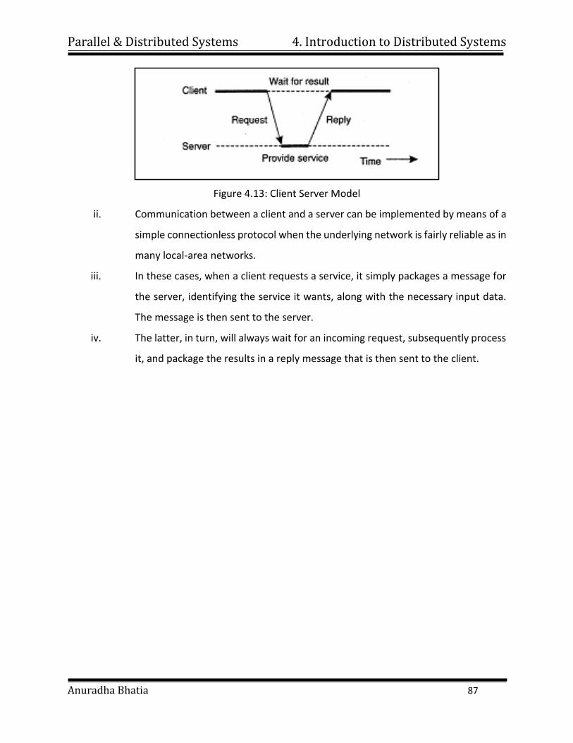
Parallel & Distributed Systems 4. Introduction to Distributed Systems
Anuradha Bhatia 87
Figure 4.13: Client Server Model
ii. Communication between a client and a server can be implemented by means of a
simple connectionless protocol when the underlying network is fairly reliable as in
many local-area networks.
iii. In these cases, when a client requests a service, it simply packages a message for
the server, identifying the service it wants, along with the necessary input data.
The message is then sent to the server.
iv. The latter, in turn, will always wait for an incoming request, subsequently process
it, and package the results in a reply message that is then sent to the client.
Parallel & Distributed Systems
Anuradha Bhatia
5. Communication CONTENTS
5.1 Layered Protocols
5.2 Remote Procedure Call
5.3 Remote Object Invocation
5.4 Message Oriented Communication
5.5 Stream Oriented Communication
Parallel & Distributed Systems 5. Communication
Anuradha Bhatia 89
1. Interprocess communication is at the heart of all distributed systems.
2. It makes no sense to study distributed systems without carefully examining the
ways that processes on different machines can exchange information.
3. Communication in distributed systems is always based on low-level message
passing as offered by the underlying network.
4. Expressing communication through message passing is harder than using
primitives based on shared memory, as available for non-distributed platforms.
5. Modem distributed systems often consist of thousands or even millions of
processes scattered across a network with unreliable communication such as the
Internet.
6. Unless the primitive communication facilities of computer networks are replaced
by something else, development of large-scale distributed applications is
extremely difficult.
5.1 Layered Protocols
1. Due to the absence of shared memory, all communication in distributed systems
is based on sending and receiving (low level) messages.
2. When process A wants to communicate with process B, it first builds a message in
its own address space.
3. Then.it executes a system call that causes the operating system to send the
message over the network to B.
4. Although this basic idea sounds simple enough, in order to prevent chaos, A and
B have to agree on the meaning of the bits being sent.
5. If A sends a brilliant new novel written in French and encoded in IBM's EBCDIC
character code, and B expects the inventory of a supermarket written in English
and encoded in ASCII, communication will be less than optimal.
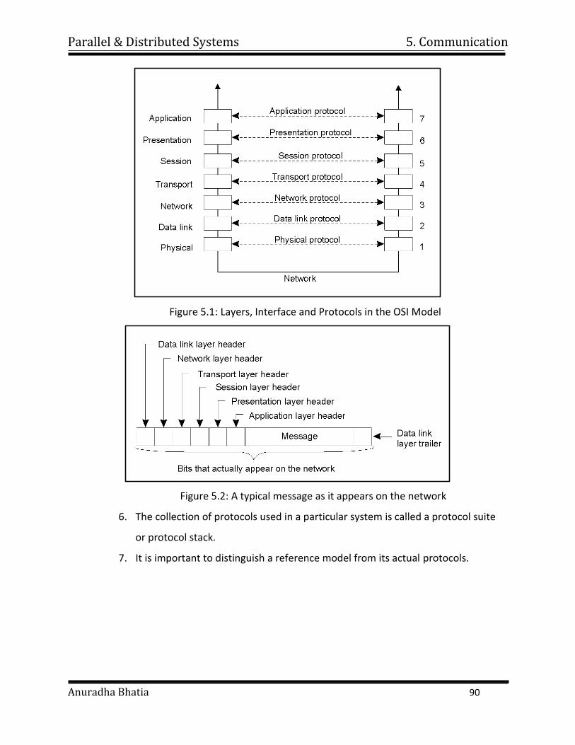
Parallel & Distributed Systems 5. Communication
Anuradha Bhatia 90
Figure 5.1: Layers, Interface and Protocols in the OSI Model
Figure 5.2: A typical message as it appears on the network
6. The collection of protocols used in a particular system is called a protocol suite
or protocol stack.
7. It is important to distinguish a reference model from its actual protocols.
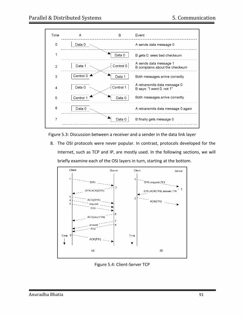
Parallel & Distributed Systems 5. Communication
Anuradha Bhatia 91
Figure 5.3: Discussion between a receiver and a sender in the data link layer
8. The OSI protocols were never popular. In contrast, protocols developed for the
Internet, such as TCP and IP, are mostly used. In the following sections, we will
briefly examine each of the OSI layers in turn, starting at the bottom.
Figure 5.4: Client-Server TCP
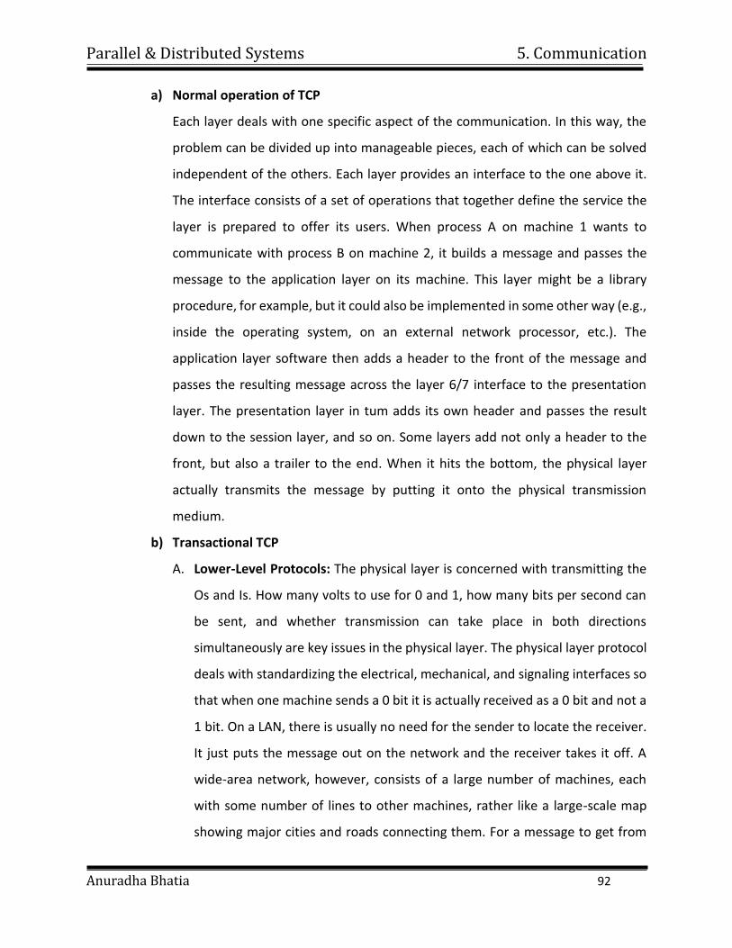
Parallel & Distributed Systems 5. Communication
Anuradha Bhatia 92
a) Normal operation of TCP
Each layer deals with one specific aspect of the communication. In this way, the
problem can be divided up into manageable pieces, each of which can be solved
independent of the others. Each layer provides an interface to the one above it.
The interface consists of a set of operations that together define the service the
layer is prepared to offer its users. When process A on machine 1 wants to
communicate with process B on machine 2, it builds a message and passes the
message to the application layer on its machine. This layer might be a library
procedure, for example, but it could also be implemented in some other way (e.g.,
inside the operating system, on an external network processor, etc.). The
application layer software then adds a header to the front of the message and
passes the resulting message across the layer 6/7 interface to the presentation
layer. The presentation layer in tum adds its own header and passes the result
down to the session layer, and so on. Some layers add not only a header to the
front, but also a trailer to the end. When it hits the bottom, the physical layer
actually transmits the message by putting it onto the physical transmission
medium.
b) Transactional TCP
A. Lower-Level Protocols: The physical layer is concerned with transmitting the
Os and Is. How many volts to use for 0 and 1, how many bits per second can
be sent, and whether transmission can take place in both directions
simultaneously are key issues in the physical layer. The physical layer protocol
deals with standardizing the electrical, mechanical, and signaling interfaces so
that when one machine sends a 0 bit it is actually received as a 0 bit and not a
1 bit. On a LAN, there is usually no need for the sender to locate the receiver.
It just puts the message out on the network and the receiver takes it off. A
wide-area network, however, consists of a large number of machines, each
with some number of lines to other machines, rather like a large-scale map
showing major cities and roads connecting them. For a message to get from
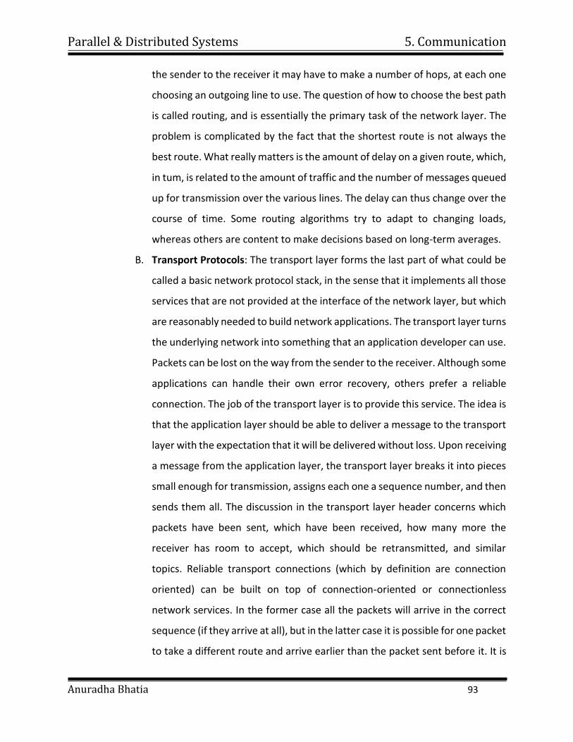
Parallel & Distributed Systems 5. Communication
Anuradha Bhatia 93
the sender to the receiver it may have to make a number of hops, at each one
choosing an outgoing line to use. The question of how to choose the best path
is called routing, and is essentially the primary task of the network layer. The
problem is complicated by the fact that the shortest route is not always the
best route. What really matters is the amount of delay on a given route, which,
in tum, is related to the amount of traffic and the number of messages queued
up for transmission over the various lines. The delay can thus change over the
course of time. Some routing algorithms try to adapt to changing loads,
whereas others are content to make decisions based on long-term averages.
B. Transport Protocols: The transport layer forms the last part of what could be
called a basic network protocol stack, in the sense that it implements all those
services that are not provided at the interface of the network layer, but which
are reasonably needed to build network applications. The transport layer turns
the underlying network into something that an application developer can use.
Packets can be lost on the way from the sender to the receiver. Although some
applications can handle their own error recovery, others prefer a reliable
connection. The job of the transport layer is to provide this service. The idea is
that the application layer should be able to deliver a message to the transport
layer with the expectation that it will be delivered without loss. Upon receiving
a message from the application layer, the transport layer breaks it into pieces
small enough for transmission, assigns each one a sequence number, and then
sends them all. The discussion in the transport layer header concerns which
packets have been sent, which have been received, how many more the
receiver has room to accept, which should be retransmitted, and similar
topics. Reliable transport connections (which by definition are connection
oriented) can be built on top of connection-oriented or connectionless
network services. In the former case all the packets will arrive in the correct
sequence (if they arrive at all), but in the latter case it is possible for one packet
to take a different route and arrive earlier than the packet sent before it. It is
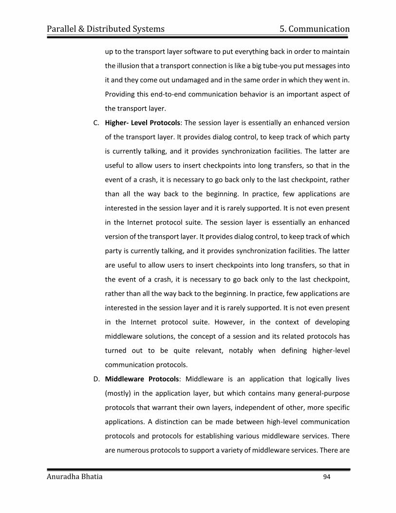
Parallel & Distributed Systems 5. Communication
Anuradha Bhatia 94
up to the transport layer software to put everything back in order to maintain
the illusion that a transport connection is like a big tube-you put messages into
it and they come out undamaged and in the same order in which they went in.
Providing this end-to-end communication behavior is an important aspect of
the transport layer.
C. Higher- Level Protocols: The session layer is essentially an enhanced version
of the transport layer. It provides dialog control, to keep track of which party
is currently talking, and it provides synchronization facilities. The latter are
useful to allow users to insert checkpoints into long transfers, so that in the
event of a crash, it is necessary to go back only to the last checkpoint, rather
than all the way back to the beginning. In practice, few applications are
interested in the session layer and it is rarely supported. It is not even present
in the Internet protocol suite. The session layer is essentially an enhanced
version of the transport layer. It provides dialog control, to keep track of which
party is currently talking, and it provides synchronization facilities. The latter
are useful to allow users to insert checkpoints into long transfers, so that in
the event of a crash, it is necessary to go back only to the last checkpoint,
rather than all the way back to the beginning. In practice, few applications are
interested in the session layer and it is rarely supported. It is not even present
in the Internet protocol suite. However, in the context of developing
middleware solutions, the concept of a session and its related protocols has
turned out to be quite relevant, notably when defining higher-level
communication protocols.
D. Middleware Protocols: Middleware is an application that logically lives
(mostly) in the application layer, but which contains many general-purpose
protocols that warrant their own layers, independent of other, more specific
applications. A distinction can be made between high-level communication
protocols and protocols for establishing various middleware services. There
are numerous protocols to support a variety of middleware services. There are
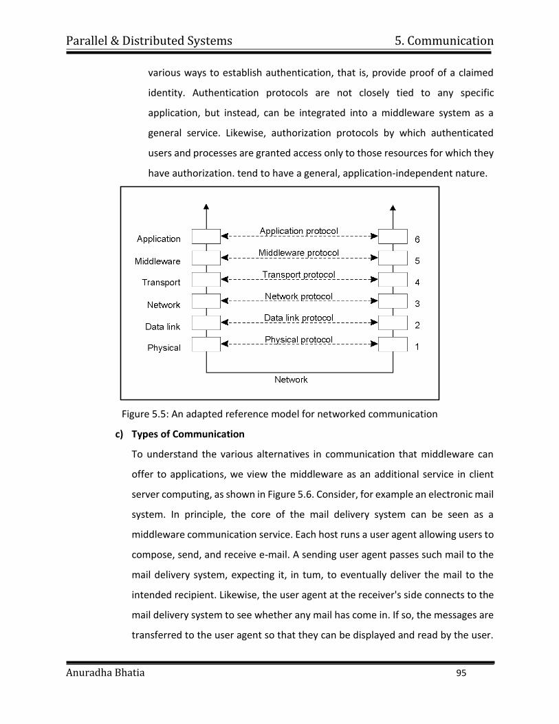
Parallel & Distributed Systems 5. Communication
Anuradha Bhatia 95
various ways to establish authentication, that is, provide proof of a claimed
identity. Authentication protocols are not closely tied to any specific
application, but instead, can be integrated into a middleware system as a
general service. Likewise, authorization protocols by which authenticated
users and processes are granted access only to those resources for which they
have authorization. tend to have a general, application-independent nature.
Figure 5.5: An adapted reference model for networked communication
c) Types of Communication
To understand the various alternatives in communication that middleware can
offer to applications, we view the middleware as an additional service in client
server computing, as shown in Figure 5.6. Consider, for example an electronic mail
system. In principle, the core of the mail delivery system can be seen as a
middleware communication service. Each host runs a user agent allowing users to
compose, send, and receive e-mail. A sending user agent passes such mail to the
mail delivery system, expecting it, in tum, to eventually deliver the mail to the
intended recipient. Likewise, the user agent at the receiver's side connects to the
mail delivery system to see whether any mail has come in. If so, the messages are
transferred to the user agent so that they can be displayed and read by the user.
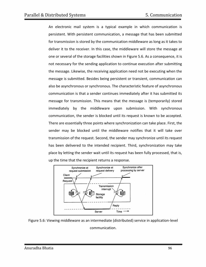
Parallel & Distributed Systems 5. Communication
Anuradha Bhatia 96
An electronic mail system is a typical example in which communication is
persistent. With persistent communication, a message that has been submitted
for transmission is stored by the communication middleware as long as it takes to
deliver it to the receiver. In this case, the middleware will store the message at
one or several of the storage facilities shown in Figure 5.6. As a consequence, it is
not necessary for the sending application to continue execution after submitting
the message. Likewise, the receiving application need not be executing when the
message is submitted. Besides being persistent or transient, communication can
also be asynchronous or synchronous. The characteristic feature of asynchronous
communication is that a sender continues immediately after it has submitted its
message for transmission. This means that the message is (temporarily) stored
immediately by the middleware upon submission. With synchronous
communication, the sender is blocked until its request is known to be accepted.
There are essentially three points where synchronization can take place. First, the
sender may be blocked until the middleware notifies that it will take over
transmission of the request. Second, the sender may synchronize until its request
has been delivered to the intended recipient. Third, synchronization may take
place by letting the sender wait until its request has been fully processed, that is,
up the time that the recipient returns a response.
Figure 5.6: Viewing middleware as an intermediate (distributed) service in application-level
communication.
Parallel & Distributed Systems 5. Communication
Anuradha Bhatia 97
5.2 Remote Procedure Call
1. Distributed systems have been based on explicit message exchange between
processes.
2. The procedures send and receive do not conceal communication at all, which is
important to achieve access transparency in distributed systems.
3. When a process on machine A calls' a procedure on machine B, the calling process
on A is suspended, and execution of the called procedure takes place on B.
Information can be transported from the caller to the callee in the parameters and
can come back in the procedure result. No message passing at all is visible to the
programmer. This method is known as Remote Procedure Call, or often just RPC.
A. Basic RPC Operation
To understand the basic operation of RPC we need to first understand the
conventional procedure call i.e the single machine call and then split the call
to a client and server part that can be executed on different machines.
i. Conventional Procedure Call: To understand the conventional procedure
call, consider the example
count = trial (fd, buf, nbytes)
Where fd is an .integer indicating a file, buf is an array of characters into
which data are read, and nbytes is another integer telling how many bytes
to read.
Several things are worth noting. For one, in C, parameters can be call-by
value or call-by-reference. A value parameter, such as fd or n bytes, is
simply copied to the stack as shown in Figure 5.7(b). To the called
procedure, a value parameter is just an initialized local variable. The called
procedure may modify it, but such changes do not affect the original value
at the calling side. A reference parameter in C is a pointer to a variable (i.e.,
the address of the variable), rather than the value of the variable. In the
call to read. The second parameter is a reference parameter because
arrays are always passed by reference in C. What is actually pushed onto
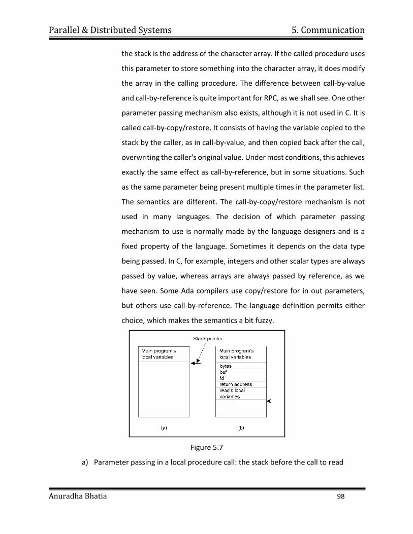
Parallel & Distributed Systems 5. Communication
Anuradha Bhatia 98
the stack is the address of the character array. If the called procedure uses
this parameter to store something into the character array, it does modify
the array in the calling procedure. The difference between call-by-value
and call-by-reference is quite important for RPC, as we shall see. One other
parameter passing mechanism also exists, although it is not used in C. It is
called call-by-copy/restore. It consists of having the variable copied to the
stack by the caller, as in call-by-value, and then copied back after the call,
overwriting the caller's original value. Under most conditions, this achieves
exactly the same effect as call-by-reference, but in some situations. Such
as the same parameter being present multiple times in the parameter list.
The semantics are different. The call-by-copy/restore mechanism is not
used in many languages. The decision of which parameter passing
mechanism to use is normally made by the language designers and is a
fixed property of the language. Sometimes it depends on the data type
being passed. In C, for example, integers and other scalar types are always
passed by value, whereas arrays are always passed by reference, as we
have seen. Some Ada compilers use copy/restore for in out parameters,
but others use call-by-reference. The language definition permits either
choice, which makes the semantics a bit fuzzy.
Figure 5.7
a) Parameter passing in a local procedure call: the stack before the call to read
Parallel & Distributed Systems 5. Communication
Anuradha Bhatia 99
b) The stack while the called procedure is active
ii. Client and Server Stubs: The idea behind RPC is to make a remote
procedure call look as much as possible like a local one. In other words, we
want RPC to be transparent-the calling procedure should not be aware that
the called procedure is executing on a different machine or vice versa. It
packs the parameters into a message and requests that message to be sent
to the server as illustrated below. Following the call to send, the client stub
calls receive, blocking itself until the reply comes back. RPC achieves its
transparency in an analogous way. When read is actually a remote
procedure (e.g., one that will run on the file server's machine), a different
version of read, called a client stub, is put into the library. Like the original
one, it, too, is called using the calling sequence of Figure 5.7 (b). Also like
the original one, it too, does a call to the local operating system. Only
unlike the original one, it does not ask the operating system to give it data.
Instead, it packs the parameters into a message and requests that message
to be sent to the server as illustrated in Figure 5.8. Following the call to
send, the client stub calls receive, blocking itself until the reply comes back.
When the message arrives at the server, the server's operating system
passes it up to a server stub. A server stub is the server-side equivalent of
a client stub: it is a piece of code that transforms requests coming in over
the network into local procedure calls. Typically the server stub will have
called receive and be blocked waiting for incoming messages. The server
stub unpacks the parameters from the message and then calls the server
procedure in the usual way. From the server's point of view, it is as though
it is being called directly by the client-the parameters and return address
are all on the stack where they belong and nothing seems unusual. The
server performs its work and then returns the result to the caller in the
usual way. For example, in the case of read, the server will fill the buffer,
pointed to by the second parameter, with the data. This buffer will be
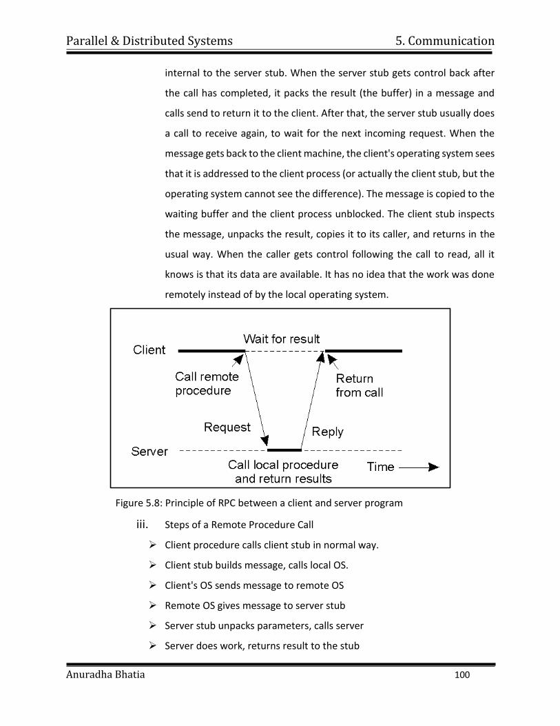
Parallel & Distributed Systems 5. Communication
Anuradha Bhatia 100
internal to the server stub. When the server stub gets control back after
the call has completed, it packs the result (the buffer) in a message and
calls send to return it to the client. After that, the server stub usually does
a call to receive again, to wait for the next incoming request. When the
message gets back to the client machine, the client's operating system sees
that it is addressed to the client process (or actually the client stub, but the
operating system cannot see the difference). The message is copied to the
waiting buffer and the client process unblocked. The client stub inspects
the message, unpacks the result, copies it to its caller, and returns in the
usual way. When the caller gets control following the call to read, all it
knows is that its data are available. It has no idea that the work was done
remotely instead of by the local operating system.
Figure 5.8: Principle of RPC between a client and server program
iii. Steps of a Remote Procedure Call
Client procedure calls client stub in normal way.
Client stub builds message, calls local OS.
Client's OS sends message to remote OS
Remote OS gives message to server stub
Server stub unpacks parameters, calls server
Server does work, returns result to the stub
Parallel & Distributed Systems 5. Communication
Anuradha Bhatia 101
Server stub packs it in message, calls local OS
Server's OS sends message to client's OS
Client's OS gives message to client stub
Stub unpacks result, returns to client
B. Parameter Passing
i. The function of the client stub is to take its parameters, pack them into a
message, and send them to the server stub.
ii. While this sounds straightforward, it is not quite as simple as it at first
appears. In this section we will look at some of the issues concerned with
parameter passing in RPC systems.
iii. Passing Value Parameters: Packing parameters into a message is called
parameter marshaling. As a very simple example, consider a remote
procedure, add(i, j), that takes two integer parameters i and j and returns
their arithmetic sum as a result. The call to add, is shown in the left-hand
portion (in the client process) in Figure 5.8. The client stub takes its two
parameters and puts them in a message as indicated, it also puts the name
or number of the procedure to be called in the message because the server
might support several different calls, and it has to be told which one is
required. When the message arrives at the server, the stub examines the
message to see which procedure is needed and then makes the
appropriate call. If the server also supports other remote procedures, the
server stub might have a switch statement in it to select the procedure to
be called, depending on the first field of the message. The actual call from
the stub to the server looks like the original client call, except that the
parameters are variables initialized from the incoming message. When the
server has finished, the server stub gains control again. It takes the result
sent back by the server and packs it into a message. This message is sent
back to back to the client stub which unpacks it to extract the result and
returns the value to the waiting client procedure.
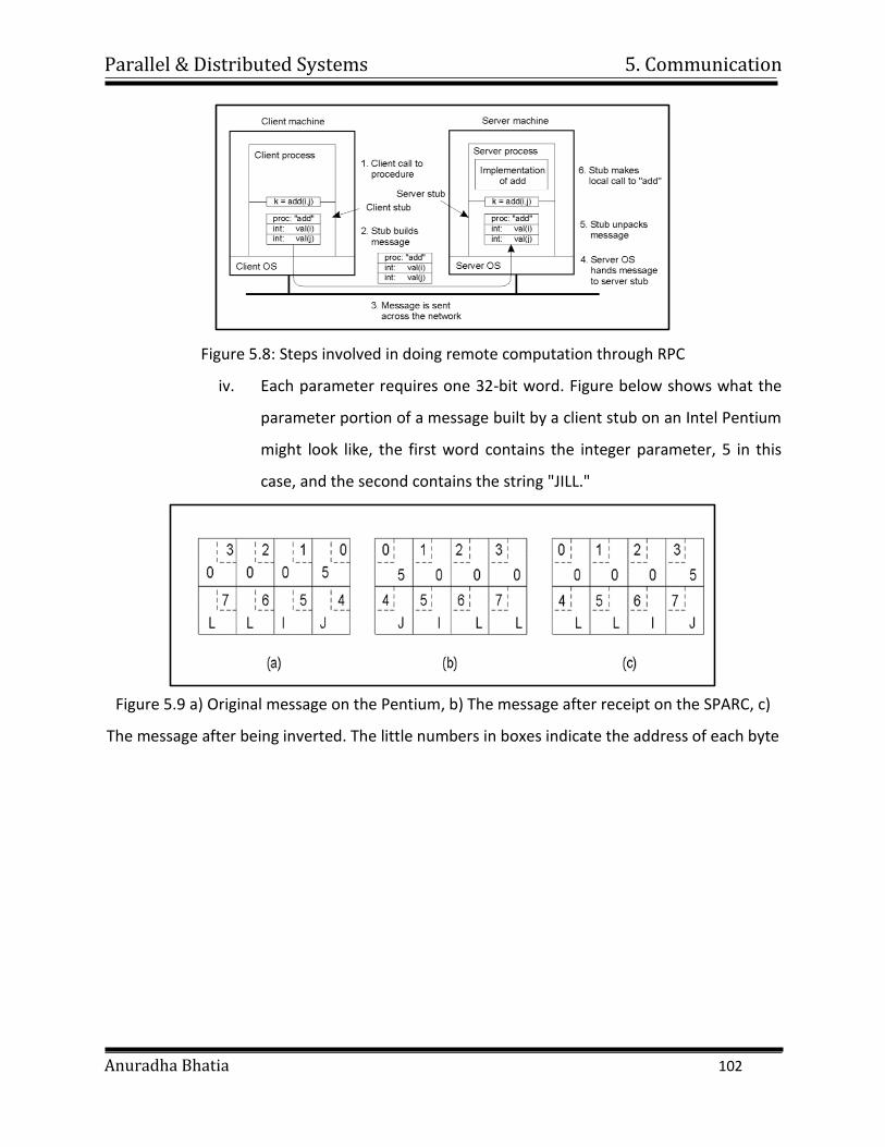
Parallel & Distributed Systems 5. Communication
Anuradha Bhatia 102
Figure 5.8: Steps involved in doing remote computation through RPC
iv. Each parameter requires one 32-bit word. Figure below shows what the
parameter portion of a message built by a client stub on an Intel Pentium
might look like, the first word contains the integer parameter, 5 in this
case, and the second contains the string "JILL."
Figure 5.9 a) Original message on the Pentium, b) The message after receipt on the SPARC, c)
The message after being inverted. The little numbers in boxes indicate the address of each byte
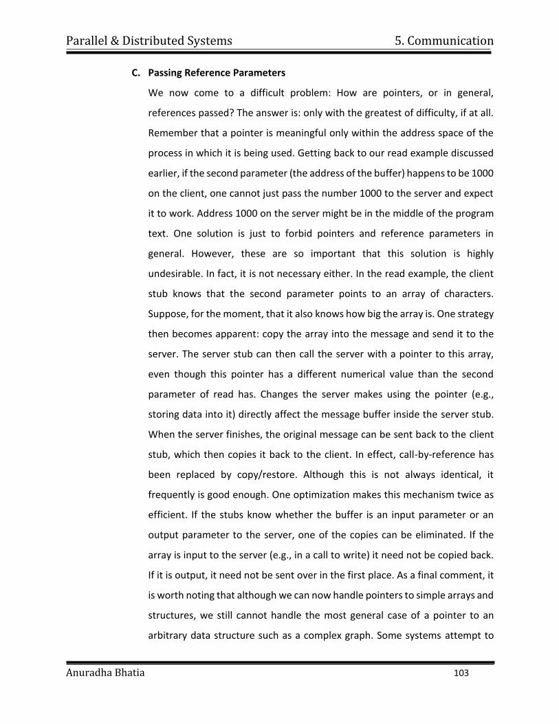
Parallel & Distributed Systems 5. Communication
Anuradha Bhatia 103
C. Passing Reference Parameters
We now come to a difficult problem: How are pointers, or in general,
references passed? The answer is: only with the greatest of difficulty, if at all.
Remember that a pointer is meaningful only within the address space of the
process in which it is being used. Getting back to our read example discussed
earlier, if the second parameter (the address of the buffer) happens to be 1000
on the client, one cannot just pass the number 1000 to the server and expect
it to work. Address 1000 on the server might be in the middle of the program
text. One solution is just to forbid pointers and reference parameters in
general. However, these are so important that this solution is highly
undesirable. In fact, it is not necessary either. In the read example, the client
stub knows that the second parameter points to an array of characters.
Suppose, for the moment, that it also knows how big the array is. One strategy
then becomes apparent: copy the array into the message and send it to the
server. The server stub can then call the server with a pointer to this array,
even though this pointer has a different numerical value than the second
parameter of read has. Changes the server makes using the pointer (e.g.,
storing data into it) directly affect the message buffer inside the server stub.
When the server finishes, the original message can be sent back to the client
stub, which then copies it back to the client. In effect, call-by-reference has
been replaced by copy/restore. Although this is not always identical, it
frequently is good enough. One optimization makes this mechanism twice as
efficient. If the stubs know whether the buffer is an input parameter or an
output parameter to the server, one of the copies can be eliminated. If the
array is input to the server (e.g., in a call to write) it need not be copied back.
If it is output, it need not be sent over in the first place. As a final comment, it
is worth noting that although we can now handle pointers to simple arrays and
structures, we still cannot handle the most general case of a pointer to an
arbitrary data structure such as a complex graph. Some systems attempt to
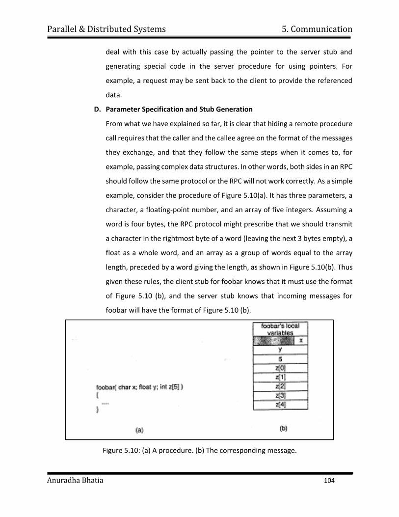
Parallel & Distributed Systems 5. Communication
Anuradha Bhatia 104
deal with this case by actually passing the pointer to the server stub and
generating special code in the server procedure for using pointers. For
example, a request may be sent back to the client to provide the referenced
data.
D. Parameter Specification and Stub Generation
From what we have explained so far, it is clear that hiding a remote procedure
call requires that the caller and the callee agree on the format of the messages
they exchange, and that they follow the same steps when it comes to, for
example, passing complex data structures. In other words, both sides in an RPC
should follow the same protocol or the RPC will not work correctly. As a simple
example, consider the procedure of Figure 5.10(a). It has three parameters, a
character, a floating-point number, and an array of five integers. Assuming a
word is four bytes, the RPC protocol might prescribe that we should transmit
a character in the rightmost byte of a word (leaving the next 3 bytes empty), a
float as a whole word, and an array as a group of words equal to the array
length, preceded by a word giving the length, as shown in Figure 5.10(b). Thus
given these rules, the client stub for foobar knows that it must use the format
of Figure 5.10 (b), and the server stub knows that incoming messages for
foobar will have the format of Figure 5.10 (b).
Figure 5.10: (a) A procedure. (b) The corresponding message.
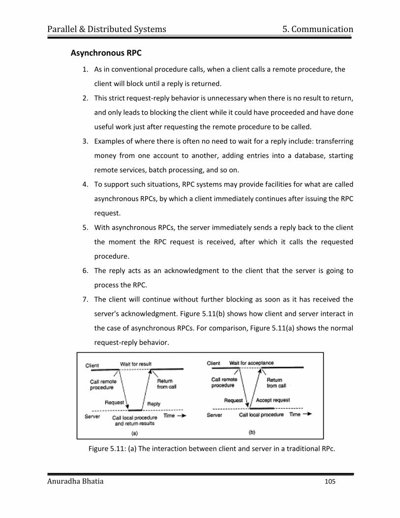
Parallel & Distributed Systems 5. Communication
Anuradha Bhatia 105
Asynchronous RPC
1. As in conventional procedure calls, when a client calls a remote procedure, the
client will block until a reply is returned.
2. This strict request-reply behavior is unnecessary when there is no result to return,
and only leads to blocking the client while it could have proceeded and have done
useful work just after requesting the remote procedure to be called.
3. Examples of where there is often no need to wait for a reply include: transferring
money from one account to another, adding entries into a database, starting
remote services, batch processing, and so on.
4. To support such situations, RPC systems may provide facilities for what are called
asynchronous RPCs, by which a client immediately continues after issuing the RPC
request.
5. With asynchronous RPCs, the server immediately sends a reply back to the client
the moment the RPC request is received, after which it calls the requested
procedure.
6. The reply acts as an acknowledgment to the client that the server is going to
process the RPC.
7. The client will continue without further blocking as soon as it has received the
server's acknowledgment. Figure 5.11(b) shows how client and server interact in
the case of asynchronous RPCs. For comparison, Figure 5.11(a) shows the normal
request-reply behavior.
Figure 5.11: (a) The interaction between client and server in a traditional RPc.
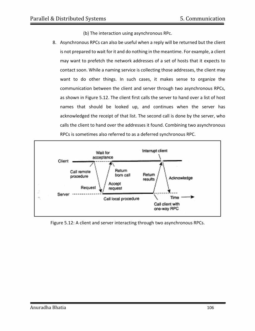
Parallel & Distributed Systems 5. Communication
Anuradha Bhatia 106
(b) The interaction using asynchronous RPc.
8. Asynchronous RPCs can also be useful when a reply will be returned but the client
is not prepared to wait for it and do nothing in the meantime. For example, a client
may want to prefetch the network addresses of a set of hosts that it expects to
contact soon. While a naming service is collecting those addresses, the client may
want to do other things. In such cases, it makes sense to organize the
communication between the client and server through two asynchronous RPCs,
as shown in Figure 5.12. The client first calls the server to hand over a list of host
names that should be looked up, and continues when the server has
acknowledged the receipt of that list. The second call is done by the server, who
calls the client to hand over the addresses it found. Combining two asynchronous
RPCs is sometimes also referred to as a deferred synchronous RPC.
Figure 5.12: A client and server interacting through two asynchronous RPCs.
Parallel & Distributed Systems 5. Communication
Anuradha Bhatia 107
5.3 Message Oriented Communication
1. Remote procedure calls and remote object invocations contribute to hiding
communication in distributed systems, that is, they enhance access transparency.
2. Unfortunately, neither mechanism is always appropriate.
3. When the receiving side is executing at the time a request is issued, alternative
communication services are needed.
4. Likewise, the inherent synchronous nature of RPCs, by which a client is blocked
until its request has been processed, sometimes needs to be replaced by
something else.
A. Message-Oriented Transient Communication: Many distributed systems and
applications are built directly on top of the simple message-oriented model
offered by the transport layer. To better understand and appreciate the
message-oriented systems as part of middleware solutions, we first discuss
messaging through transport-level sockets.
i. Berkeley Sockets: Special attention has been paid to standardizing the
interface of the transport layer to allow programmers to make use of its
entire suite of (messaging) protocols through a simple set of primitives.
Also, standard interfaces make it easier to port an application to a different
machine. The listen primitive is called only in the case of connection-
oriented communication. It is a non-blocking call that allows the local
operating system to reserve enough buffers for a specified maximum
number of connections that the caller is willing to accept. A call to accept
blocks the caller until a connection request arrives. When a request arrives,
the local operating system creates a new socket with the same properties
as the original one, and returns it to the caller. This approach will allow the
server to, for example, fork off a process that will subsequently handle the
actual communication through the new connection. The server, in the
meantime, can go back and wait for another connection request on the
original socket. a socket must first be created using the socket primitive,
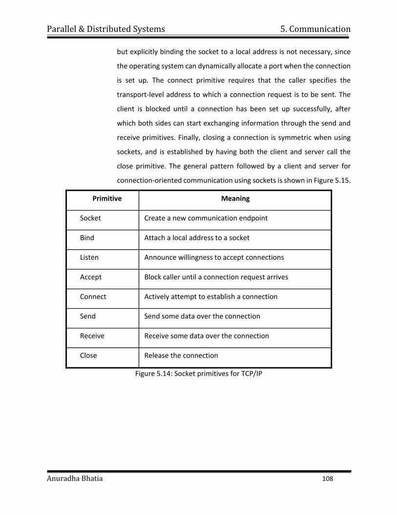
Parallel & Distributed Systems 5. Communication
Anuradha Bhatia 108
but explicitly binding the socket to a local address is not necessary, since
the operating system can dynamically allocate a port when the connection
is set up. The connect primitive requires that the caller specifies the
transport-level address to which a connection request is to be sent. The
client is blocked until a connection has been set up successfully, after
which both sides can start exchanging information through the send and
receive primitives. Finally, closing a connection is symmetric when using
sockets, and is established by having both the client and server call the
close primitive. The general pattern followed by a client and server for
connection-oriented communication using sockets is shown in Figure 5.15.
Primitive Meaning
Socket Create a new communication endpoint
Bind Attach a local address to a socket
Listen Announce willingness to accept connections
Accept Block caller until a connection request arrives
Connect Actively attempt to establish a connection
Send Send some data over the connection
Receive Receive some data over the connection
Close Release the connection
Figure 5.14: Socket primitives for TCP/IP
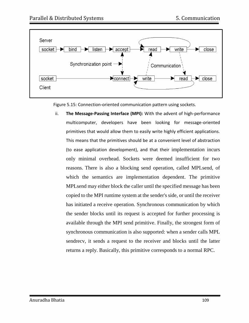
Parallel & Distributed Systems 5. Communication
Anuradha Bhatia 109
Figure 5.15: Connection-oriented communication pattern using sockets.
ii. The Message-Passing Interface (MPI): With the advent of high-performance
multicomputer, developers have been looking for message-oriented
primitives that would allow them to easily write highly efficient applications.
This means that the primitives should be at a convenient level of abstraction
(to ease application development), and that their implementation incurs
only minimal overhead. Sockets were deemed insufficient for two
reasons. There is also a blocking send operation, called MPLsend, of
which the semantics are implementation dependent. The primitive
MPLsend may either block the caller until the specified message has been
copied to the MPI runtime system at the sender's side, or until the receiver
has initiated a receive operation. Synchronous communication by which
the sender blocks until its request is accepted for further processing is
available through the MPI send primitive. Finally, the strongest form of
synchronous communication is also supported: when a sender calls MPL
sendrecv, it sends a request to the receiver and blocks until the latter
returns a reply. Basically, this primitive corresponds to a normal RPC.
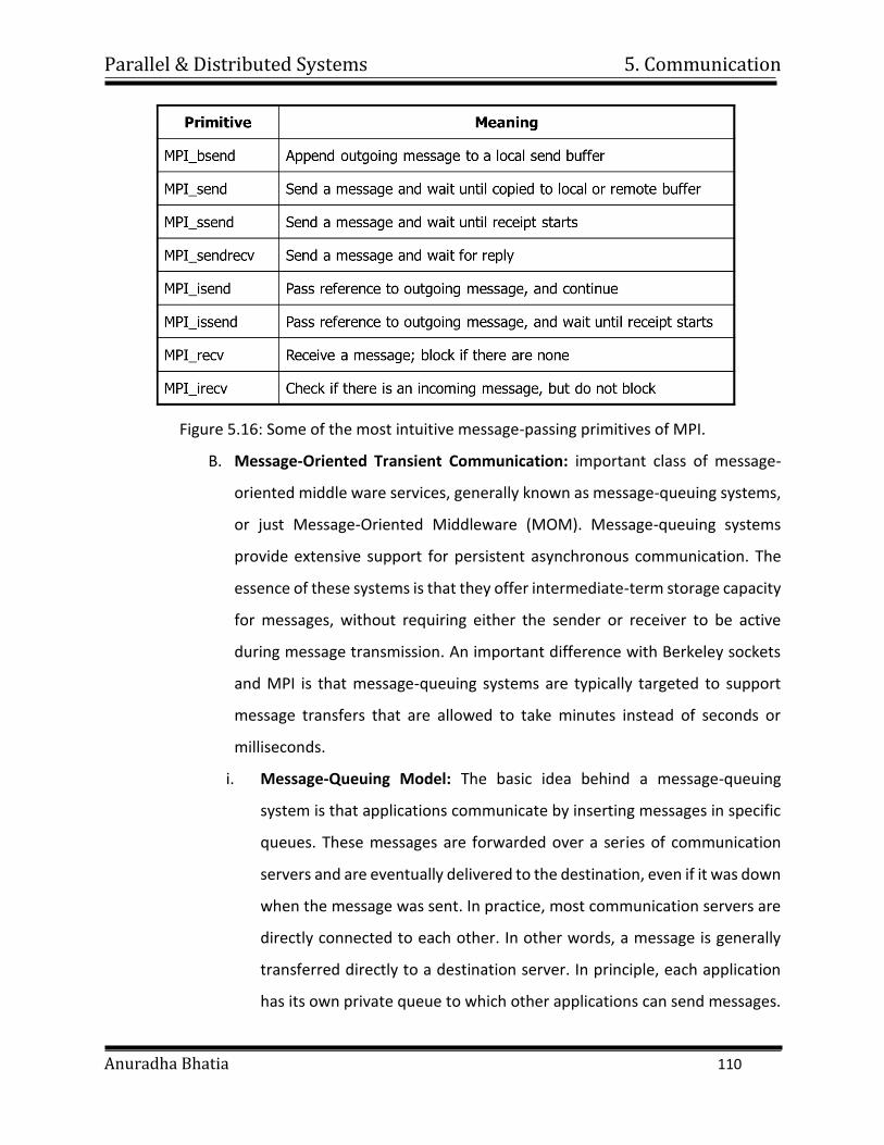
Parallel & Distributed Systems 5. Communication
Anuradha Bhatia 110
Figure 5.16: Some of the most intuitive message-passing primitives of MPI.
B. Message-Oriented Transient Communication: important class of message-
oriented middle ware services, generally known as message-queuing systems,
or just Message-Oriented Middleware (MOM). Message-queuing systems
provide extensive support for persistent asynchronous communication. The
essence of these systems is that they offer intermediate-term storage capacity
for messages, without requiring either the sender or receiver to be active
during message transmission. An important difference with Berkeley sockets
and MPI is that message-queuing systems are typically targeted to support
message transfers that are allowed to take minutes instead of seconds or
milliseconds.
i. Message-Queuing Model: The basic idea behind a message-queuing
system is that applications communicate by inserting messages in specific
queues. These messages are forwarded over a series of communication
servers and are eventually delivered to the destination, even if it was down
when the message was sent. In practice, most communication servers are
directly connected to each other. In other words, a message is generally
transferred directly to a destination server. In principle, each application
has its own private queue to which other applications can send messages.
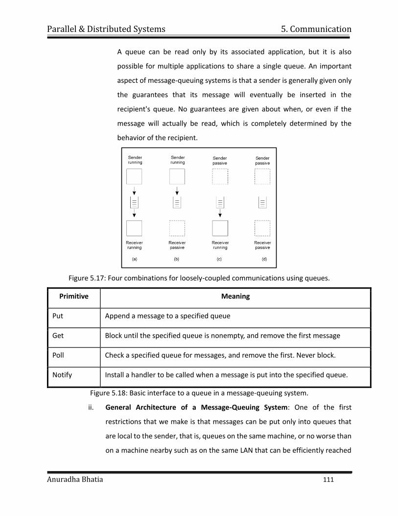
Parallel & Distributed Systems 5. Communication
Anuradha Bhatia 111
A queue can be read only by its associated application, but it is also
possible for multiple applications to share a single queue. An important
aspect of message-queuing systems is that a sender is generally given only
the guarantees that its message will eventually be inserted in the
recipient's queue. No guarantees are given about when, or even if the
message will actually be read, which is completely determined by the
behavior of the recipient.
Figure 5.17: Four combinations for loosely-coupled communications using queues.
Primitive Meaning
Put Append a message to a specified queue
Get Block until the specified queue is nonempty, and remove the first message
Poll Check a specified queue for messages, and remove the first. Never block.
Notify Install a handler to be called when a message is put into the specified queue.
Figure 5.18: Basic interface to a queue in a message-queuing system.
ii. General Architecture of a Message-Queuing System: One of the first
restrictions that we make is that messages can be put only into queues that
are local to the sender, that is, queues on the same machine, or no worse than
on a machine nearby such as on the same LAN that can be efficiently reached
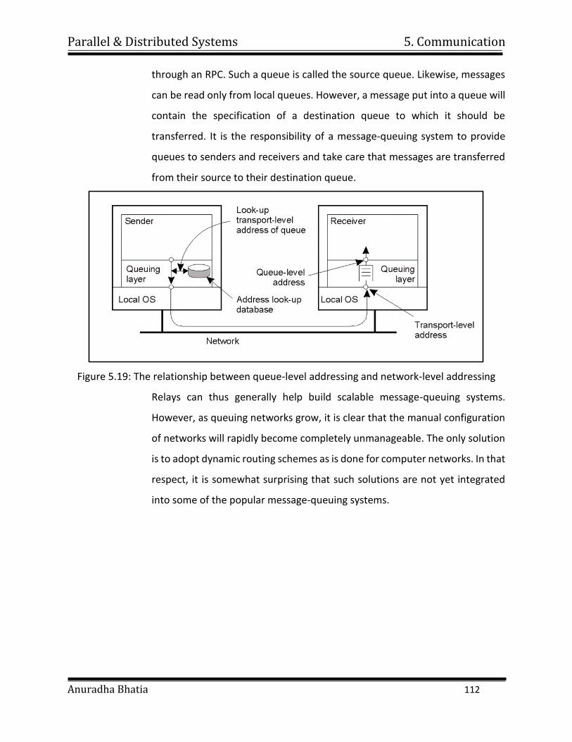
Parallel & Distributed Systems 5. Communication
Anuradha Bhatia 112
through an RPC. Such a queue is called the source queue. Likewise, messages
can be read only from local queues. However, a message put into a queue will
contain the specification of a destination queue to which it should be
transferred. It is the responsibility of a message-queuing system to provide
queues to senders and receivers and take care that messages are transferred
from their source to their destination queue.
Figure 5.19: The relationship between queue-level addressing and network-level addressing
Relays can thus generally help build scalable message-queuing systems.
However, as queuing networks grow, it is clear that the manual configuration
of networks will rapidly become completely unmanageable. The only solution
is to adopt dynamic routing schemes as is done for computer networks. In that
respect, it is somewhat surprising that such solutions are not yet integrated
into some of the popular message-queuing systems.
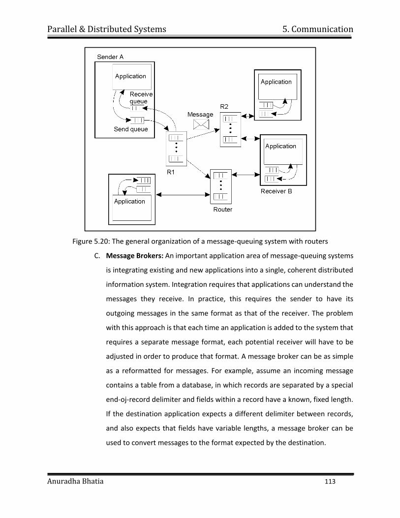
Parallel & Distributed Systems 5. Communication
Anuradha Bhatia 113
Figure 5.20: The general organization of a message-queuing system with routers
C. Message Brokers: An important application area of message-queuing systems
is integrating existing and new applications into a single, coherent distributed
information system. Integration requires that applications can understand the
messages they receive. In practice, this requires the sender to have its
outgoing messages in the same format as that of the receiver. The problem
with this approach is that each time an application is added to the system that
requires a separate message format, each potential receiver will have to be
adjusted in order to produce that format. A message broker can be as simple
as a reformatted for messages. For example, assume an incoming message
contains a table from a database, in which records are separated by a special
end-oj-record delimiter and fields within a record have a known, fixed length.
If the destination application expects a different delimiter between records,
and also expects that fields have variable lengths, a message broker can be
used to convert messages to the format expected by the destination.
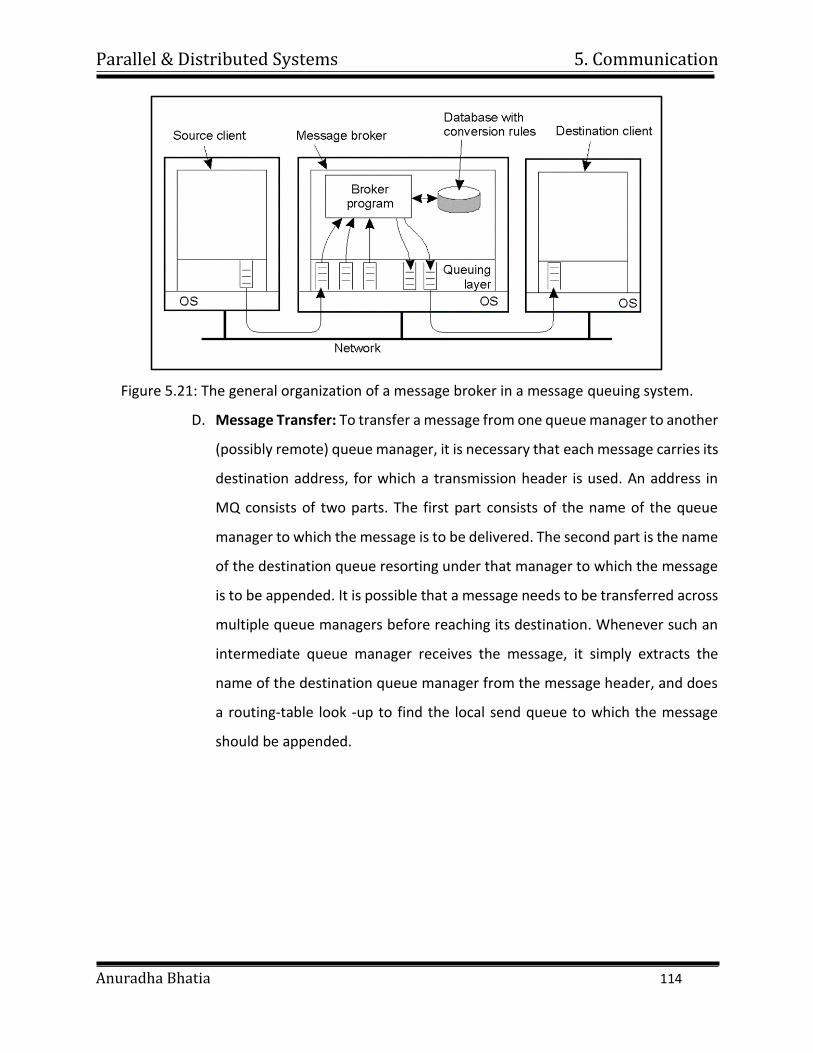
Parallel & Distributed Systems 5. Communication
Anuradha Bhatia 114
Figure 5.21: The general organization of a message broker in a message queuing system.
D. Message Transfer: To transfer a message from one queue manager to another
(possibly remote) queue manager, it is necessary that each message carries its
destination address, for which a transmission header is used. An address in
MQ consists of two parts. The first part consists of the name of the queue
manager to which the message is to be delivered. The second part is the name
of the destination queue resorting under that manager to which the message
is to be appended. It is possible that a message needs to be transferred across
multiple queue managers before reaching its destination. Whenever such an
intermediate queue manager receives the message, it simply extracts the
name of the destination queue manager from the message header, and does
a routing-table look -up to find the local send queue to which the message
should be appended.
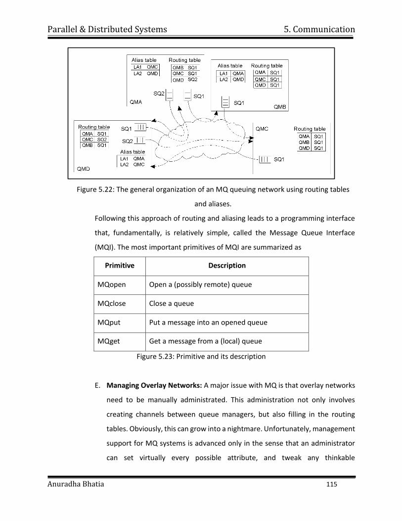
Parallel & Distributed Systems 5. Communication
Anuradha Bhatia 115
Figure 5.22: The general organization of an MQ queuing network using routing tables
and aliases.
Following this approach of routing and aliasing leads to a programming interface
that, fundamentally, is relatively simple, called the Message Queue Interface
(MQI). The most important primitives of MQI are summarized as
Primitive Description
MQopen Open a (possibly remote) queue
MQclose Close a queue
MQput Put a message into an opened queue
MQget Get a message from a (local) queue
Figure 5.23: Primitive and its description
E. Managing Overlay Networks: A major issue with MQ is that overlay networks
need to be manually administrated. This administration not only involves
creating channels between queue managers, but also filling in the routing
tables. Obviously, this can grow into a nightmare. Unfortunately, management
support for MQ systems is advanced only in the sense that an administrator
can set virtually every possible attribute, and tweak any thinkable
Parallel & Distributed Systems 5. Communication
Anuradha Bhatia 116
configuration. At the heart of overlay management is the channel control
function component, which logically sits between message channel agents.
This component allows an operator to monitor exactly what is going on at two
end points of a channel. In addition, it is used to create channels and routing
tables, but also to manage the queue managers that host the message channel
agents. In a way, this approach to overlay management strongly resembles the
management of cluster servers where a single administration server is used.
5.4 Stream Oriented Communication
1. There are also forms of communication in which timing plays a crucial role.
2. Considering, an audio stream built up as a sequence of 16-bit samples, each
representing the amplitude of the sound wave as is done through Pulse Code
Modulation (PCM).
3. Assuming that the audio stream represents CD quality, meaning that the original
sound wave has been sampled at a frequency of 44,100 Hz. To reproduce the
original sound, it is essential that the samples in the audio stream are played out
in the order they appear in the stream, but also at intervals of exactly 1/44,100
sec.
4. Playing out at a different rate will produce an incorrect version of the original
sound.
A. Support for Continuous Media: Support for the exchange of time-dependent
information is often formulated as support for continuous media. A medium
refers to the means by which information is conveyed. These means include
storage and transmission media, presentation media such as a monitor, and
so on. An important type of medium is the way that information is
represented. In other words, how is information encoded in a computer
system? Different representations are used for different types of information.
For example, text is generally encoded as ASCII or Unicode. Images can be
represented in different formats such as GIF or lPEG. Audio streams can be
encoded in a computer system by, for example, taking 16-bit samples using
Parallel & Distributed Systems 5. Communication
Anuradha Bhatia 117
PCM. In continuous (representation) media, the temporal relationships
between different data items are fundamental to correctly interpreting what
the data actually means. We already gave an example of reproducing a sound
wave by playing out an audio stream. As another example, consider motion.
Motion can be represented by a series of images in which successive images
must be displayed at a uniform spacing T in time, typically 30-40 msec per
image. Correct reproduction requires not only showing the stills in the correct
order, but also at a constant frequency of liT images per second. In contrast to
continuous media, discrete (representation) media, is characterized by the
fact that temporal relationships between data items are not fundamental to
correctly interpreting the data. Typical examples of discrete media include
representations of text and still images, but also object code or executable
files.
B. Data Stream: To capture the exchange of time-dependent information,
distributed systems generally provide support for data streams. A data stream
is nothing but a sequence of data units. Data streams can be applied to
discrete as well as continuous media. For example, UNIX pipes or TCPIIP
connections are typical examples of (byte-oriented) discrete data streams.
Playing an audio file typically requires setting up a continuous data stream
between the file and the audio device. To capture the exchange of time-
dependent information, distributed systems generally provide support for
data streams. A data stream is nothing but a sequence of data units. Data
streams can be applied to discrete as well as continuous media. For example,
UNIX pipes or TCPIIP connections are typical examples of (byte-oriented)
discrete data streams. Playing an audio file typically requires setting up a
continuous data stream between the file and the audio device. Streams can be
simple or complex. A simple stream consists of only a single sequence of data,
whereas a complex stream consists of several related simple streams, called
sub streams. The relation between the sub streams in a complex stream is
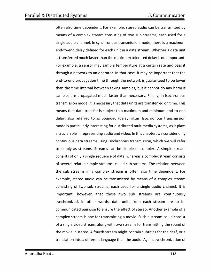
Parallel & Distributed Systems 5. Communication
Anuradha Bhatia 118
often also time dependent. For example, stereo audio can be transmitted by
means of a complex stream consisting of two sub streams, each used for a
single audio channel. In synchronous transmission mode, there is a maximum
end-to-end delay defined for each unit in a data stream. Whether a data unit
is transferred much faster than the maximum tolerated delay is not important.
For example, a sensor may sample temperature at a certain rate and pass it
through a network to an operator. In that case, it may be important that the
end-to-end propagation time through the network is guaranteed to be lower
than the time interval between taking samples, but it cannot do any harm if
samples are propagated much faster than necessary. Finally, in isochronous
transmission mode, it is necessary that data units are transferred on time. This
means that data transfer is subject to a maximum and minimum end-to-end
delay, also referred to as bounded (delay) jitter. Isochronous transmission
mode is particularly interesting for distributed multimedia systems, as it plays
a crucial role in representing audio and video. In this chapter, we consider only
continuous data streams using isochronous transmission, which we will refer
to simply as streams. Streams can be simple or complex. A simple stream
consists of only a single sequence of data, whereas a complex stream consists
of several related simple streams, called sub streams. The relation between
the sub streams in a complex stream is often also time dependent. For
example, stereo audio can be transmitted by means of a complex stream
consisting of two sub streams, each used for a single audio channel. It is
important, however, that those two sub streams are continuously
synchronized. In other words, data units from each stream are to be
communicated pairwise to ensure the effect of stereo. Another example of a
complex stream is one for transmitting a movie. Such a stream could consist
of a single video stream, along with two streams for transmitting the sound of
the movie in stereo. A fourth stream might contain subtitles for the deaf, or a
translation into a different language than the audio. Again, synchronization of
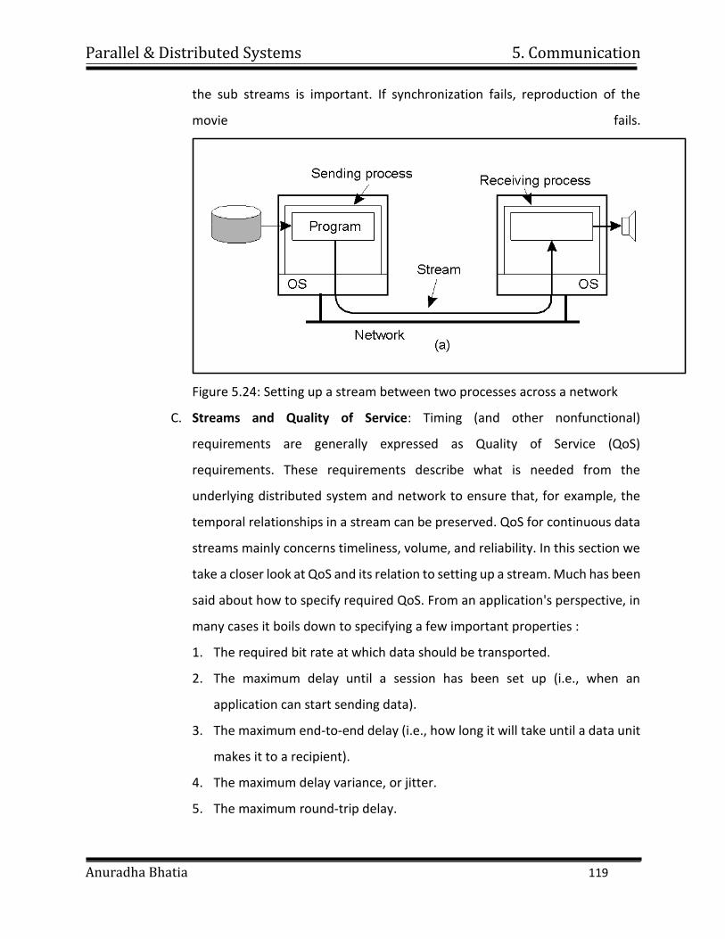
Parallel & Distributed Systems 5. Communication
Anuradha Bhatia 119
the sub streams is important. If synchronization fails, reproduction of the
movie fails.
Figure 5.24: Setting up a stream between two processes across a network
C. Streams and Quality of Service: Timing (and other nonfunctional)
requirements are generally expressed as Quality of Service (QoS)
requirements. These requirements describe what is needed from the
underlying distributed system and network to ensure that, for example, the
temporal relationships in a stream can be preserved. QoS for continuous data
streams mainly concerns timeliness, volume, and reliability. In this section we
take a closer look at QoS and its relation to setting up a stream. Much has been
said about how to specify required QoS. From an application's perspective, in
many cases it boils down to specifying a few important properties :
1. The required bit rate at which data should be transported.
2. The maximum delay until a session has been set up (i.e., when an
application can start sending data).
3. The maximum end-to-end delay (i.e., how long it will take until a data unit
makes it to a recipient).
4. The maximum delay variance, or jitter.
5. The maximum round-trip delay.
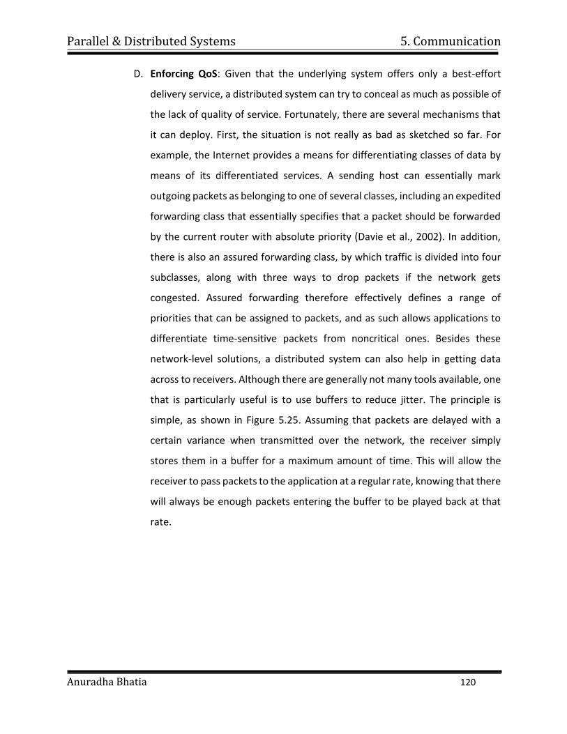
Parallel & Distributed Systems 5. Communication
Anuradha Bhatia 120
D. Enforcing QoS: Given that the underlying system offers only a best-effort
delivery service, a distributed system can try to conceal as much as possible of
the lack of quality of service. Fortunately, there are several mechanisms that
it can deploy. First, the situation is not really as bad as sketched so far. For
example, the Internet provides a means for differentiating classes of data by
means of its differentiated services. A sending host can essentially mark
outgoing packets as belonging to one of several classes, including an expedited
forwarding class that essentially specifies that a packet should be forwarded
by the current router with absolute priority (Davie et al., 2002). In addition,
there is also an assured forwarding class, by which traffic is divided into four
subclasses, along with three ways to drop packets if the network gets
congested. Assured forwarding therefore effectively defines a range of
priorities that can be assigned to packets, and as such allows applications to
differentiate time-sensitive packets from noncritical ones. Besides these
network-level solutions, a distributed system can also help in getting data
across to receivers. Although there are generally not many tools available, one
that is particularly useful is to use buffers to reduce jitter. The principle is
simple, as shown in Figure 5.25. Assuming that packets are delayed with a
certain variance when transmitted over the network, the receiver simply
stores them in a buffer for a maximum amount of time. This will allow the
receiver to pass packets to the application at a regular rate, knowing that there
will always be enough packets entering the buffer to be played back at that
rate.
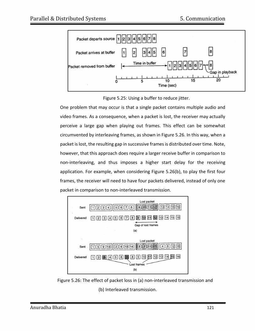
Parallel & Distributed Systems 5. Communication
Anuradha Bhatia 121
Figure 5.25: Using a buffer to reduce jitter.
One problem that may occur is that a single packet contains multiple audio and
video frames. As a consequence, when a packet is lost, the receiver may actually
perceive a large gap when playing out frames. This effect can be somewhat
circumvented by interleaving frames, as shown in Figure 5.26. In this way, when a
packet is lost, the resulting gap in successive frames is distributed over time. Note,
however, that this approach does require a larger receive buffer in comparison to
non-interleaving, and thus imposes a higher start delay for the receiving
application. For example, when considering Figure 5.26(b), to play the first four
frames, the receiver will need to have four packets delivered, instead of only one
packet in comparison to non-interleaved transmission.
Figure 5.26: The effect of packet loss in (a) non-interleaved transmission and
(b) Interleaved transmission.
Parallel & Distributed Systems 5. Communication
Anuradha Bhatia 122
5.5 Stream Synchronization
1. An important issue in multimedia systems is that different streams, possibly in the
form of a complex stream, are mutually synchronized.
2. Synchronization of streams deals with maintaining temporal relations between
streams.
3. Two types of synchronization occur. The simplest form of synchronization is that
between a discrete data stream and a continuous data stream. Consider, for
example, a slide show on the Web that has been enhanced with audio. Each slide
is transferred from the server to the client in the form of a discrete data stream.
4. At the same time, the client should play out a specific (part of an) audio stream
that matches the current slide that is also fetched from the server.
5. In this case, the audio stream is to be 'synchronized with the presentation of slides.
A more demanding type of synchronization is that between continuous data
streams.
6. A daily example is playing a movie in which the video stream needs to be
synchronized with the audio, commonly referred to as lip synchronization.
7. Another example of synchronization is playing a stereo audio stream consisting of
two sub streams, one for each channel.
8. Proper play out requires that the two sub streams are tightly synchronized: a
difference of more than 20 usee can distort the stereo effect.
5.6 Multicast communication
1. An important topic in communication in distributed systems is the support for
sending data to multiple receivers, also known as multicast communication.
2. For many years, this topic has belonged to the domain of network protocols,
where numerous proposals for network-level and transport-level solutions have
been implemented and evaluated.
3. A major issue in all solutions was setting up the communication paths for
information dissemination.
Parallel & Distributed Systems 5. Communication
Anuradha Bhatia 123
4. In practice, this involved a huge management effort, in many cases requiring
human intervention.
5. In addition, as long as there is no convergence of proposals, ISPs have shown to
be reluctant to support multicasting. With the advent of peer-to-peer technology,
and notably structured overlay management, it became easier to set up
communication paths.
6. As peer-to-peer solutions are typically deployed at the application layer, various
application-level multicasting techniques have been introduced. In this section,
we will take a brief look at these techniques.
7. Multicast communication can also be accomplished in other ways than setting up
explicit communication paths.
8. As we also explore in this section. Gossip-based information dissemination
provides simple (yet often less efficient) ways for multicasting.
Parallel & Distributed Systems
Anuradha Bhatia
6. Resource and Process Management
CONTENTS
6.1 Desirable Features of global Scheduling algorithm
6.2 Task assignment approach
6.3 Load balancing approach
6.4 Load sharing approach
6.5 Introduction to process management
6.6 Process migration
6.7 Threads
6.8 Virtualization
6.9 Clients, Servers, Code Migration
Parallel & Distributed Systems 6. Resource and Process Management
Anuradha Bhatia 125
A resource can be a logical, such as a shared file, or physical, such as a CPU (a node of the
distributed system). One of the functions of a distributed operating system is to assign
processes to the nodes (resources) of the distributed system such that the resource
usage, response time, network congestion, and scheduling overhead are optimized.
There are three techniques for scheduling processes of a distributed system:
1. Task Assignment Approach, in which each process submitted by a user for
processing is viewed as a collection of related tasks and these tasks are scheduled
to suitable nodes so as to improve performance.
2. Load-balancing approach, in which all the processes submitted by the users are
distributed among the nodes of the system so as to equalize the workload among
the nodes.
3. Load-sharing approach, which simply attempts to conserve the ability of the
system to perform work by assuring that no node is idle while processes wait for
being processed.
The task assignment approach has limited applicability to practical situations
because it works on the assumption that the characteristics (e.g. execution time, IPC costs
etc) of all the processes to be scheduled are known in advance.
6.1 Desirable features of a good global scheduling algorithm
i. No a priori knowledge about the processes: Scheduling algorithms that operate
based on the information about the characteristics and resource requirements of
the processes pose an extra burden on the users who must provide this
information while submitting their processes for execution.
ii. Dynamic in nature: Process assignment decisions should be dynamic, I.e., be
based on the current load of the system and not on some static policy. It is
recommended that the scheduling algorithm possess the flexibility to migrate a
process more than once because the initial decision of placing a process on a
particular node may have to be changed after some time to adapt to the new
system load.
Parallel & Distributed Systems 6. Resource and Process Management
Anuradha Bhatia 126
iii. Quick decision making capability: Heuristic methods requiring less computational
efforts (and hence less time) while providing near-optimal results are preferable
to exhaustive (optimal) solution methods.
iv. Balanced system performance and scheduling overhead: Algorithms that provide
near-optimal system performance with a minimum of global state information
(such as CPU load) gathering overhead are desirable. This is because the overhead
increases as the amount of global state information collected increases. This is
because the usefulness of that information is decreased due to both the aging of
the information being gathered and the low scheduling frequency as a result of
the cost of gathering and processing the extra information.
v. Stability: Fruitless migration of processes, known as processor thrashing, must be
prevented. E.g. if nodes n1 and n2 observe that node n3 is idle and then offload a
portion of their work to n3 without being aware of the offloading decision made
by the other node. Now if n3 becomes overloaded due to this it may again start
transferring its processes to other nodes. This is caused by scheduling decisions
being made at each node independently of decisions made by other nodes.
vi. Scalability: A scheduling algorithm should scale well as the number of nodes
increases. An algorithm that makes scheduling decisions by first inquiring the
workload from all the nodes and then selecting the most lightly loaded node has
poor scalability. This will work fine only when there are few nodes in the system.
This is because the inquirer receives a flood of replies almost simultaneously, and
the time required to process the reply messages for making a node selection is too
long as the number of nodes (N) increase. Also the network traffic quickly
consumes network bandwidth. A simple approach is to probe only m of N nodes
for selecting a node.
vii. Fault tolerance: A good scheduling algorithm should not be disabled by the crash
of one or more nodes of the system. Also, if the nodes are partitioned into two or
more groups due to link failures, the algorithm should be capable of functioning
properly for the nodes within a group. Algorithms that have decentralized decision
Parallel & Distributed Systems 6. Resource and Process Management
Anuradha Bhatia 127
making capability and consider only available nodes in their decision making have
better fault tolerance capability.
viii. Fairness of service: Global scheduling policies that blindly attempt to balance the
load on all the nodes of the system are not good from the point of view of fairness
of service. This is because in any load-balancing scheme, heavily loaded nodes will
obtain all the benefits while lightly loaded nodes will suffer poorer response time
than in a stand-alone configuration. A fair strategy that improves response time
of the former without unduly affecting the latter is desirable. Hence load-
balancing has to be replaced by the concept of load sharing, that is, a node will
share some of its resources as long as its users are not significantly affected.
6.2 Task Assignment Approach
1. A process has already been split up into pieces called tasks. This split occurs along
natural boundaries (such as a method), so that each task will have integrity in itself
and data transfers among the tasks are minimized.
2. The amount of computation required by each task and the speed of each CPU are
known.
3. The cost of processing each task on every node is known. This is derived from
assumption 2.
4. The IPC costs between every pair of tasks is known. The IPC cost is 0 for tasks
assigned to the same node. This is usually estimated by an analysis of the static
program. If two tasks communicate n times and the average time for each inter-
task communication is t, the IPC costs for the two tasks is n * t.
5. Precedence relationships among the tasks are known.
6. Reassignment of tasks is not possible.
Goal is to assign the tasks of a process to the nodes of a distributed system in such a
manner as to achieve goals such as the following goals:
Minimization of IPC costs
Quick turnaround time for the complete process
A high degree of parallelism
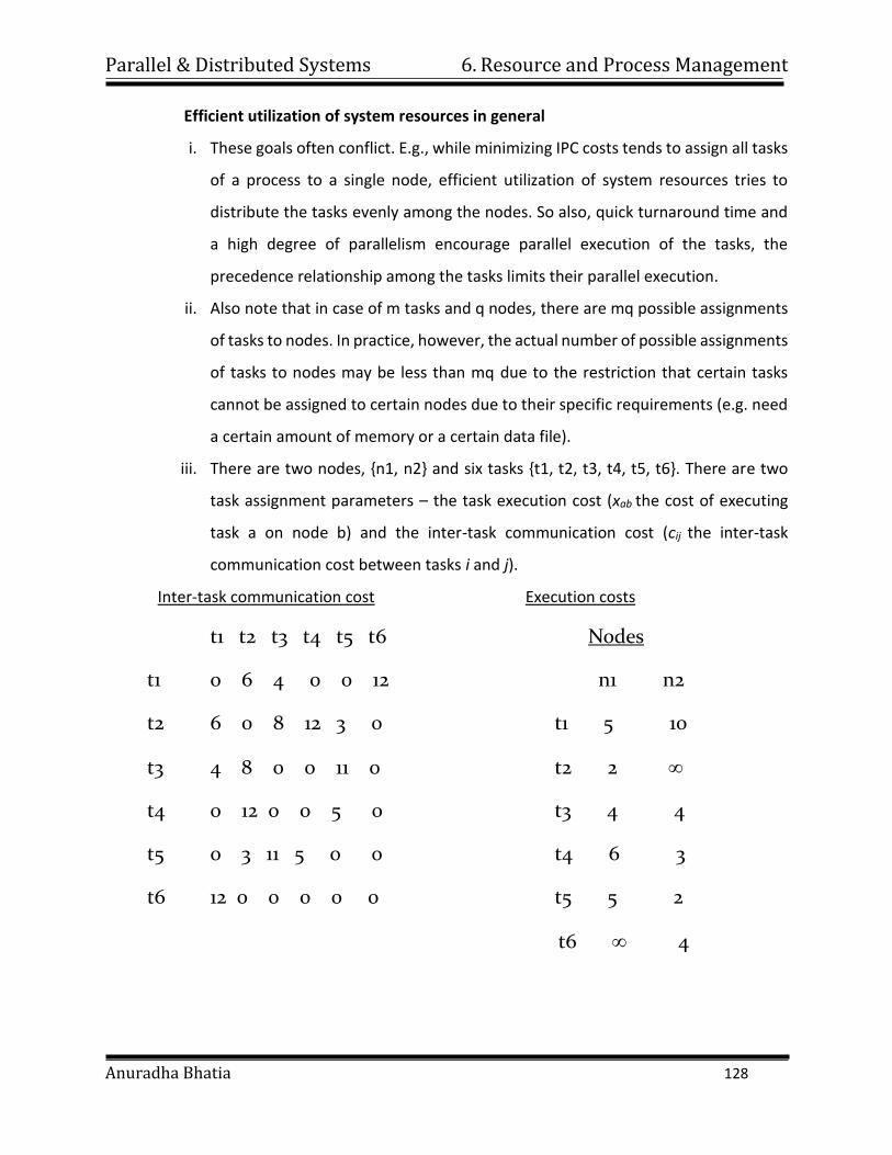
Parallel & Distributed Systems 6. Resource and Process Management
Anuradha Bhatia 128
Efficient utilization of system resources in general
i. These goals often conflict. E.g., while minimizing IPC costs tends to assign all tasks
of a process to a single node, efficient utilization of system resources tries to
distribute the tasks evenly among the nodes. So also, quick turnaround time and
a high degree of parallelism encourage parallel execution of the tasks, the
precedence relationship among the tasks limits their parallel execution.
ii. Also note that in case of m tasks and q nodes, there are mq possible assignments
of tasks to nodes. In practice, however, the actual number of possible assignments
of tasks to nodes may be less than mq due to the restriction that certain tasks
cannot be assigned to certain nodes due to their specific requirements (e.g. need
a certain amount of memory or a certain data file).
iii. There are two nodes, {n1, n2} and six tasks {t1, t2, t3, t4, t5, t6}. There are two
task assignment parameters – the task execution cost (xab the cost of executing
task a on node b) and the inter-task communication cost (cij the inter-task
communication cost between tasks i and j).
Inter-task communication cost Execution costs
t1 t2 t3 t4 t5 t6 Nodes
t1 0 6 4 0 0 12 n1 n2
t2 6 0 8 12 3 0 t1 5 10
t3 4 8 0 0 11 0 t2 2
t4 0 12 0 0 5 0 t3 4 4
t5 0 3 11 5 0 0 t4 6 3
t6 12 0 0 0 0 0 t5 5 2
t6 4
Parallel & Distributed Systems 6. Resource and Process Management
Anuradha Bhatia 129
Task t6 cannot be executed on node n1 and task t2 cannot be executed on node n2 since
the resources they need are not available on these nodes.
Task assignment example
1) Serial assignment, where tasks t1, t2, t3 are assigned to node n1 and tasks t4, t5, t6 are
assigned to node n2:
Execution cost, x = x11 + x21 + x31 + x42 + x52 + x62 = 5 + 2 + 4 + 3 + 2 + 4 = 20
Communication cost, c = c14 + c15 + c16 + c24 + c25 + c26 + c34 + c35 + c36 = 0 + 0 +
12 + 12 + 3 + 0 + 0 + 11 + 0 = 38. Hence total cost = 58.
2) Optimal assignment, where tasks t1, t2, t3, t4, t5 are assigned to node n1 and task t6 is
assigned to node n2.
Execution cost, x = x11 + x21 + x31 + x41 + x51 + x62 = 5 + 2 + 4 + 6 + 5 + 4 = 26
Communication cost, c = c16 + c26 + c36 + c46 + c56= 12 + 0 + 0 + 0 + 0 = 12
Total cost = 38
Optimal assignments are found by first creating a static assignment graph. In this graph,
the weights of the edges joining pairs of task nodes represent inter-task communication
costs. The weight on the edge joining a task node to node n1 represents the execution
cost of that task on node n2 and vice-versa. Then we determine a minimum cutset in this
graph.
A cutset is defined to be a set of edges such that when these edges are removed, the
nodes of the graph are partitioned into two disjoint subsets such that nodes in one subset
are reachable from n1 and the nodes in the other are reachable from n2. Each task node
is reachable from either n1 or n2. The weight of a cutset is the sum of the weights of the
edges in the cutset. This sums up the execution and communication costs for that
assignment. An optimal assignment is found by finding a minimum cutset.
Basic idea: Finding an optimal assignment to achieve goals such as the following:
o Minimization of IPC costs
o Quick turnaround time of process
o High degree of parallelism
Parallel & Distributed Systems 6. Resource and Process Management
Anuradha Bhatia 130
o Efficient utilization of resources
6.3 Load balancing approach
A Taxonomy of Load-Balancing Algorithms
1. Load-balancing approach
2. Load-balancing algorithms
3. Dynamic
4. Static
5. Deterministic
6. Probabilistic
7. Centralized
8. Distributed
9. Cooperative
10. Non-cooperative
1. Load-balancing approach- Type of load-balancing algorithms
i. Static versus Dynamic
Static algorithms use only information about the average behavior of the system
Static algorithms ignore the current state or load of the nodes in the system
Dynamic algorithms collect state information and react to system state if it
changed
Static algorithms are much more simpler
Dynamic algorithms are able to give significantly better performance
2. Load-balancing approach Type of static load-balancing algorithms
i. Deterministic versus Probabilistic
Deterministic algorithms use the information about the properties of the nodes
and the characteristic of processes to be scheduled
Probabilistic algorithms use information of static attributes of the system (e.g.
number of nodes, processing capability, topology) to formulate simple process
placement rules
Deterministic approach is difficult to optimize
Parallel & Distributed Systems 6. Resource and Process Management
Anuradha Bhatia 131
Probabilistic approach has poor performance
3. Load-balancing approach Type of dynamic load-balancing algorithms
i.Centralized versus Distributed
Centralized approach collects information to server node and makes assignment
decision
Distributed approach contains entities to make decisions on a predefined set of
nodes
Centralized algorithms can make efficient decisions, have lower fault-tolerance
Distributed algorithms avoid the bottleneck of collecting state information and
react faster
4. Load-balancing approach Type of distributed load-balancing algorithms
i. Cooperative versus Noncooperative
In Noncooperative algorithms entities act as autonomous ones and make
scheduling decisions independently from other entities
In Cooperative algorithms distributed entities cooperate with each other
Cooperative algorithms are more complex and involve larger overhead
Stability of Cooperative algorithms are better
5. Issues in designing Load-balancing algorithms
Load estimation policy
determines how to estimate the workload of a node
Process transfer policy
determines whether to execute a process locally or remote
State information exchange policy
determines how to exchange load information among nodes
Location policy
determines to which node the transferable process should be sent
Priority assignment policy
determines the priority of execution of local and remote processes
Migration limiting policy
Parallel & Distributed Systems 6. Resource and Process Management
Anuradha Bhatia 132
determines the total number of times a process can migrate
6. Load estimation policy I.for Load-balancing algorithms
To balance the workload on all the nodes of the system, it is necessary to decide
how to measure the workload of a particular node
Some measurable parameters (with time and node dependent factor) can be the
following:
Total number of processes on the node
Resource demands of these processes
Instruction mixes of these processes
Architecture and speed of the node’s processor
Several load-balancing algorithms use the total number of processes to achieve
big efficiency
7. Load estimation policy II.for Load-balancing algorithms
In some cases the true load could vary widely depending on the remaining service
time, which can be measured in several way:
Memoryless method assumes that all processes have the same expected
remaining service time, independent of the time used so far
Past repeats assumes that the remaining service time is equal to the time used
so far
Distribution method states that if the distribution service times is known, the
associated process’s remaining service time is the expected remaining time
conditioned by the time already used
8. Load estimation policy III.for Load-balancing algorithms
None of the previous methods can be used in modern systems because of
periodically running processes and daemons
An acceptable method for use as the load estimation policy in these systems
would be to measure the CPU utilization of the nodes
Central Processing Unit utilization is defined as the number of CPU cycles actually
executed per unit of real time
Parallel & Distributed Systems 6. Resource and Process Management
Anuradha Bhatia 133
It can be measured by setting up a timer to periodically check the CPU state
(idle/busy)
9. Process transfer policy I.for Load-balancing algorithms
Most of the algorithms use the threshold policy to decide on whether the node is
lightly-loaded or heavily-loaded
Threshold value is a limiting value of the workload of node which can be
determined by
Static policy: predefined threshold value for each node depending on
processing capability
Dynamic policy: threshold value is calculated from average workload and a
predefined constant
Below threshold value node accepts processes to execute, above threshold value
node tries to transfer processes to a lightly-loaded node
Single-threshold policy may lead to unstable algorithm because under loaded
node could turn to be overloaded right after a process migration
To reduce instability double-threshold policy has been proposed which is also
known as high-low policy
10. Process transfer policy III. for Load-balancing algorithms
Double threshold policy
When node is in overloaded region new local processes are sent to run
remotely, requests to accept remote processes are rejected
When node is in normal region new local processes run locally, requests to
accept remote processes are rejected
When node is in under loaded region new local processes run locally, requests
to accept remote processes are accepted
Parallel & Distributed Systems 6. Resource and Process Management
Anuradha Bhatia 134
11. Location policy I. for Load-balancing algorithms
Threshold method
Policy selects a random node, checks whether the node is able to receive the
process, and then transfers the process. If node rejects, another node is
selected randomly. This continues until probe limit is reached.
Shortest method
L distinct nodes are chosen at random, each is polled to determine its load.
The process is transferred to the node having the minimum value unless its
workload value prohibits to accept the process.
Simple improvement is to discontinue probing whenever a node with zero load
is encountered.
12. Location policy II. for Load-balancing algorithms
Bidding method
Nodes contain managers (to send processes) and contractors (to receive
processes)
Managers broadcast a request for bid, contractors respond with bids (prices
based on capacity of the contractor node) and manager selects the best offer
Winning contractor is notified and asked whether it accepts the process for
execution or not
Full autonomy for the nodes regarding scheduling
Big communication overhead
Difficult to decide a good pricing policy
13. Location policy III. for Load-balancing algorithms
Pairing
Contrary to the former methods the pairing policy is to reduce the variance of
load only between pairs
Each node asks some randomly chosen node to form a pair with it
If it receives a rejection it randomly selects another node and tries to pair again
Parallel & Distributed Systems 6. Resource and Process Management
Anuradha Bhatia 135
Two nodes that differ greatly in load are temporarily paired with each other
and migration starts
The pair is broken as soon as the migration is over
A node only tries to find a partner if it has at least two processes
14. State information exchange policy I. for Load-balancing algorithms
Dynamic policies require frequent exchange of state information, but these extra
messages arise two opposite impacts:
Increasing the number of messages gives more accurate scheduling decision
Increasing the number of messages raises the queuing time of messages
State information policies can be the following:
Periodic broadcast
Broadcast when state changes
On-demand exchange
Exchange by polling
15. State information exchange policy II. for Load-balancing algorithms
Periodic broadcast
Each node broadcasts its state information after the elapse of every T units of
time
Problem: heavy traffic, fruitless messages, poor scalability since information
exchange is too large for networks having many nodes
Broadcast when state changes
Avoids fruitless messages by broadcasting the state only when a process
arrives or departures
Further improvement is to broadcast only when state switches to another
region (double-threshold policy)
16. State information exchange policy III. for Load-balancing algorithms
On-demand exchange
In this method a node broadcast a State-Information-Request message when
its state switches from normal to either underloaded or overloaded region.
Parallel & Distributed Systems 6. Resource and Process Management
Anuradha Bhatia 136
On receiving this message other nodes reply with their own state information
to the requesting node
Further improvement can be that only those nodes reply which are useful to
the requesting node
Exchange by polling
To avoid poor scalability (coming from broadcast messages) the partner node
is searched by polling the other nodes on by one, until poll limit is reached
17. Priority assignment policy for Load-balancing algorithms
Selfish
Local processes are given higher priority than remote processes. Worst
response time performance of the three policies.
Altruistic
Remote processes are given higher priority than local processes. Best response
time performance of the three policies.
Intermediate
When the number of local processes is greater or equal to the number of
remote processes, local processes are given higher priority than remote
processes. Otherwise, remote processes are given higher priority than local
processes.
18. Migration limiting policy for Load-balancing algorithms
This policy determines the total number of times a process can migrate
Uncontrolled
A remote process arriving at a node is treated just as a process originating
at a node, so a process may be migrated any number of times
Controlled
Avoids the instability of the uncontrolled policy
Use a migration count parameter to fix a limit on the number of time a
process can migrate
Irrevocable migration policy: migration count is fixed to 1
Parallel & Distributed Systems 6. Resource and Process Management
Anuradha Bhatia 137
For long execution processes migration count must be greater than 1 to
adapt for dynamically changing states
6.4 Load sharing approach
Drawbacks of Load-balancing approach
Load balancing technique with attempting equalizing the workload on all the
nodes is not an appropriate object since big overhead is generated by
gathering exact state information
Load balancing is not achievable since number of processes in a node is always
fluctuating and temporal unbalance among the nodes exists every moment
Basic ideas for Load-sharing approach
It is necessary and sufficient to prevent nodes from being idle while some
other nodes have more than two processes
Load-sharing is much simpler than load-balancing since it only attempts to
ensure that no node is idle when heavily node exists
Priority assignment policy and migration limiting policy are the same as that
for the load-balancing algorithms
Load estimation policies for Load-sharing algorithms
Since load-sharing algorithms simply attempt to avoid idle nodes, it is sufficient to
know whether a node is busy or idle
Thus these algorithms normally employ the simplest load estimation policy of
counting the total number of processes
In modern systems where permanent existence of several processes on an idle
node is possible, algorithms measure CPU utilization to estimate the load of a
node
Process transfer policies for Load-sharing algorithms
Algorithms normally use all-or-nothing strategy
This strategy uses the threshold value of all the nodes fixed to 1
Nodes become receiver node when it has no process, and become sender node
when it has more than 1 process
Parallel & Distributed Systems 6. Resource and Process Management
Anuradha Bhatia 138
To avoid processing power on nodes having zero process load-sharing algorithms
use a threshold value of 2 instead of 1
When CPU utilization is used as the load estimation policy, the double-threshold
policy should be used as the process transfer policy
Location policies I. for Load-sharing algorithms
Location policy decides whether the sender node or the receiver node of the
process takes the initiative to search for suitable node in the system, and this
policy can be the following:
Sender-initiated location policy
Sender node decides where to send the process
Heavily loaded nodes search for lightly loaded nodes
Receiver-initiated location policy
Receiver node decides from where to get the process
Lightly loaded nodes search for heavily loaded nodes
Location policies II. for Load-sharing algorithms
Sender-initiated location policy
Node becomes overloaded, it either broadcasts or randomly probes the other
nodes one by one to find a node that is able to receive remote processes
When broadcasting, suitable node is known as soon as reply arrives
Receiver-initiated location policy
Nodes becomes underloaded, it either broadcast or randomly probes the
other nodes one by one to indicate its willingness to receive remote processes
Receiver-initiated policy require preemptive process migration facility since
scheduling decisions are usually made at process departure epochs
Location policies III. For Load-sharing algorithms
Experiences with location policies
Both policies gives substantial performance advantages over the situation in
which no load-sharing is attempted
Sender-initiated policy is preferable at light to moderate system loads
Parallel & Distributed Systems 6. Resource and Process Management
Anuradha Bhatia 139
Receiver-initiated policy is preferable at high system loads
Sender-initiated policy provide better performance for the case when process
transfer cost significantly more at receiver-initiated than at sender-initiated
policy due to the preemptive transfer of processes
State information exchange policies for Load-sharing algorithms
In load-sharing algorithms it is not necessary for the nodes to periodically
exchange state information, but needs to know the state of other nodes when it
is either under loaded or overloaded
Broadcast when state changes
In sender-initiated/receiver-initiated location policy a node broadcasts State
Information Request when it becomes overloaded/under loaded
It is called broadcast-when-idle policy when receiver-initiated policy is used
with fixed threshold value of 1
Poll when state changes
In large networks polling mechanism is used
Polling mechanism randomly asks different nodes for state information until
find an appropriate one or probe limit is reached
It is called poll-when-idle policy when receiver-initiated policy is used with
fixed threshold value value of 1
Resource manager of a distributed system schedules the processes to optimize
combination of resources usage, response time, network congestion, scheduling
overhead
Three different approaches has been discussed
Task assignment approach deals with the assignment of task in order to
minimize inter process communication costs and improve turnaround time for
the complete process, by taking some constraints into account
In load-balancing approach the process assignment decisions attempt to
equalize the avarage workload on all the nodes of the system
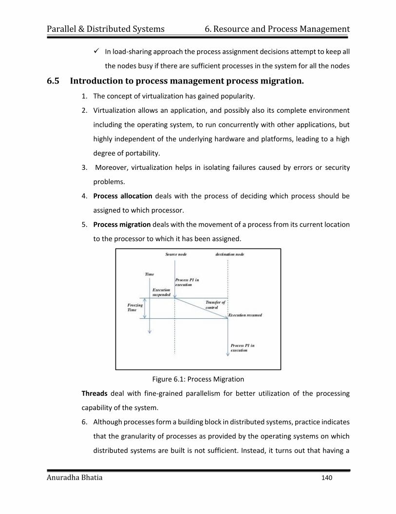
Parallel & Distributed Systems 6. Resource and Process Management
Anuradha Bhatia 140
In load-sharing approach the process assignment decisions attempt to keep all
the nodes busy if there are sufficient processes in the system for all the nodes
6.5 Introduction to process management process migration.
1. The concept of virtualization has gained popularity.
2. Virtualization allows an application, and possibly also its complete environment
including the operating system, to run concurrently with other applications, but
highly independent of the underlying hardware and platforms, leading to a high
degree of portability.
3. Moreover, virtualization helps in isolating failures caused by errors or security
problems.
4. Process allocation deals with the process of deciding which process should be
assigned to which processor.
5. Process migration deals with the movement of a process from its current location
to the processor to which it has been assigned.
Figure 6.1: Process Migration
Threads deal with fine-grained parallelism for better utilization of the processing
capability of the system.
6. Although processes form a building block in distributed systems, practice indicates
that the granularity of processes as provided by the operating systems on which
distributed systems are built is not sufficient. Instead, it turns out that having a
Parallel & Distributed Systems 6. Resource and Process Management
Anuradha Bhatia 141
finer granularity in the form of multiple threads of control per process makes it
much easier to build distributed applications and to attain better performance.
6.6 Threads
1. To execute a program, an operating system creates a number of virtual
processors, each one for running a different program.
2. To keep track of these virtual processors, the operating system has a process table,
containing entries to store CPU register values, memory maps, open files,
accounting information. Privileges, etc.
3. A process is often defined as a program in execution, that is, a program that is
currently being executed on one of the operating system's virtual processors.
4. An important issue is that the operating system takes great care to ensure that
independent processes cannot maliciously or inadvertently affect the correctness
of each other's behavior.
5. The fact that multiple processes may be concurrently sharing the same CPU and
other hardware resources is made transparent.
6. The operating system requires hardware support to enforce this separation.
7. Like a process, a thread executes its own piece of code, independently from other
threads.
8. In contrast to processes, no attempt is made to achieve a high degree of
concurrency transparency if this would result in performance degradation.
9. Therefore, a thread system generally maintains only the minimum information to
allow a CPU to be shared by several threads. In particular, a thread context often
consists of nothing more than the CPU context, along with some other information
for thread management.
10. For example, a thread system may keep track of the fact that a thread is currently
blocked on a mutex variable, so as not to select it for execution.
11. Information that is not strictly necessary to manage multiple threads is generally
ignored. For this reason, protecting data against inappropriate access by threads
within a single process is left entirely to application developers.
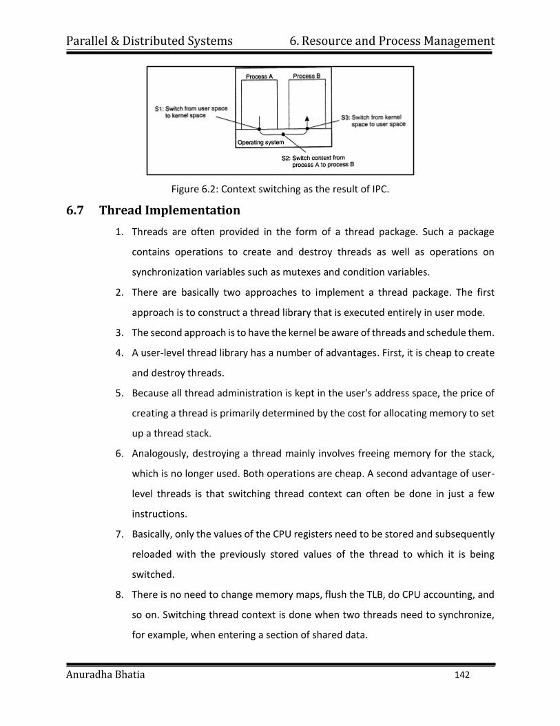
Parallel & Distributed Systems 6. Resource and Process Management
Anuradha Bhatia 142
Figure 6.2: Context switching as the result of IPC.
6.7 Thread Implementation
1. Threads are often provided in the form of a thread package. Such a package
contains operations to create and destroy threads as well as operations on
synchronization variables such as mutexes and condition variables.
2. There are basically two approaches to implement a thread package. The first
approach is to construct a thread library that is executed entirely in user mode.
3. The second approach is to have the kernel be aware of threads and schedule them.
4. A user-level thread library has a number of advantages. First, it is cheap to create
and destroy threads.
5. Because all thread administration is kept in the user's address space, the price of
creating a thread is primarily determined by the cost for allocating memory to set
up a thread stack.
6. Analogously, destroying a thread mainly involves freeing memory for the stack,
which is no longer used. Both operations are cheap. A second advantage of user-
level threads is that switching thread context can often be done in just a few
instructions.
7. Basically, only the values of the CPU registers need to be stored and subsequently
reloaded with the previously stored values of the thread to which it is being
switched.
8. There is no need to change memory maps, flush the TLB, do CPU accounting, and
so on. Switching thread context is done when two threads need to synchronize,
for example, when entering a section of shared data.
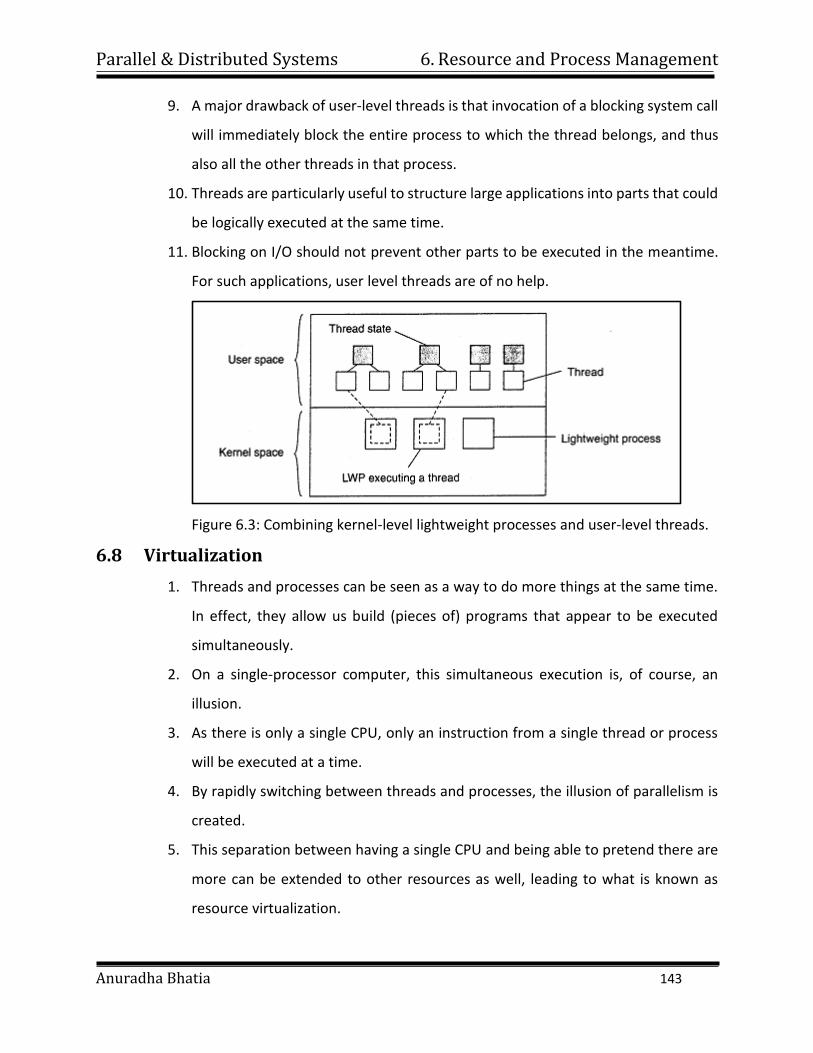
Parallel & Distributed Systems 6. Resource and Process Management
Anuradha Bhatia 143
9. A major drawback of user-level threads is that invocation of a blocking system call
will immediately block the entire process to which the thread belongs, and thus
also all the other threads in that process.
10. Threads are particularly useful to structure large applications into parts that could
be logically executed at the same time.
11. Blocking on I/O should not prevent other parts to be executed in the meantime.
For such applications, user level threads are of no help.
Figure 6.3: Combining kernel-level lightweight processes and user-level threads.
6.8 Virtualization
1. Threads and processes can be seen as a way to do more things at the same time.
In effect, they allow us build (pieces of) programs that appear to be executed
simultaneously.
2. On a single-processor computer, this simultaneous execution is, of course, an
illusion.
3. As there is only a single CPU, only an instruction from a single thread or process
will be executed at a time.
4. By rapidly switching between threads and processes, the illusion of parallelism is
created.
5. This separation between having a single CPU and being able to pretend there are
more can be extended to other resources as well, leading to what is known as
resource virtualization.
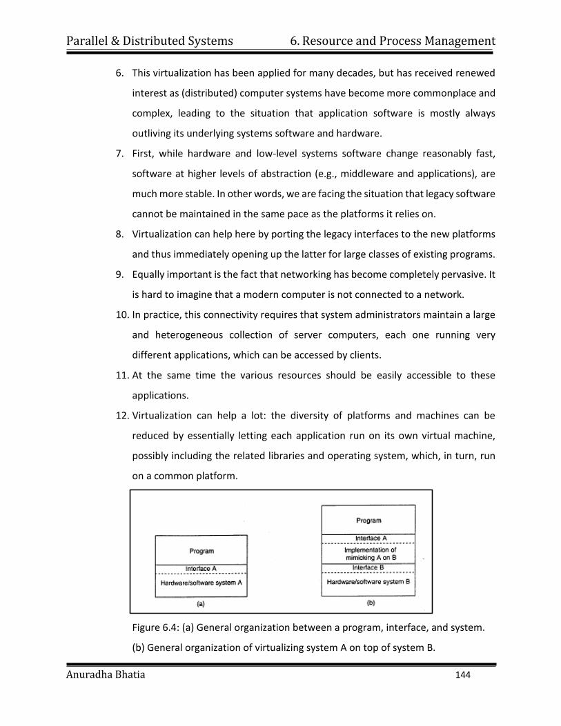
Parallel & Distributed Systems 6. Resource and Process Management
Anuradha Bhatia 144
6. This virtualization has been applied for many decades, but has received renewed
interest as (distributed) computer systems have become more commonplace and
complex, leading to the situation that application software is mostly always
outliving its underlying systems software and hardware.
7. First, while hardware and low-level systems software change reasonably fast,
software at higher levels of abstraction (e.g., middleware and applications), are
much more stable. In other words, we are facing the situation that legacy software
cannot be maintained in the same pace as the platforms it relies on.
8. Virtualization can help here by porting the legacy interfaces to the new platforms
and thus immediately opening up the latter for large classes of existing programs.
9. Equally important is the fact that networking has become completely pervasive. It
is hard to imagine that a modern computer is not connected to a network.
10. In practice, this connectivity requires that system administrators maintain a large
and heterogeneous collection of server computers, each one running very
different applications, which can be accessed by clients.
11. At the same time the various resources should be easily accessible to these
applications.
12. Virtualization can help a lot: the diversity of platforms and machines can be
reduced by essentially letting each application run on its own virtual machine,
possibly including the related libraries and operating system, which, in turn, run
on a common platform.
Figure 6.4: (a) General organization between a program, interface, and system.
(b) General organization of virtualizing system A on top of system B.
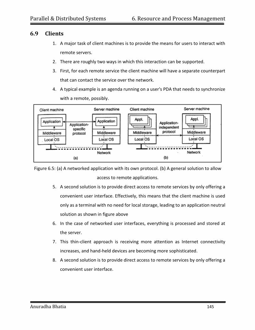
Parallel & Distributed Systems 6. Resource and Process Management
Anuradha Bhatia 145
6.9 Clients
1. A major task of client machines is to provide the means for users to interact with
remote servers.
2. There are roughly two ways in which this interaction can be supported.
3. First, for each remote service the client machine will have a separate counterpart
that can contact the service over the network.
4. A typical example is an agenda running on a user's PDA that needs to synchronize
with a remote, possibly.
Figure 6.5: (a) A networked application with its own protocol. (b) A general solution to allow
access to remote applications.
5. A second solution is to provide direct access to remote services by only offering a
convenient user interface. Effectively, this means that the client machine is used
only as a terminal with no need for local storage, leading to an application neutral
solution as shown in figure above
6. In the case of networked user interfaces, everything is processed and stored at
the server.
7. This thin-client approach is receiving more attention as Internet connectivity
increases, and hand-held devices are becoming more sophisticated.
8. A second solution is to provide direct access to remote services by only offering a
convenient user interface.
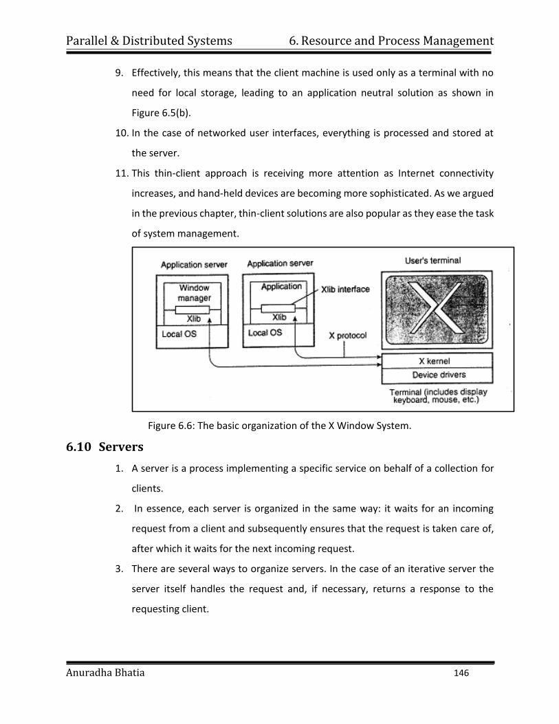
Parallel & Distributed Systems 6. Resource and Process Management
Anuradha Bhatia 146
9. Effectively, this means that the client machine is used only as a terminal with no
need for local storage, leading to an application neutral solution as shown in
Figure 6.5(b).
10. In the case of networked user interfaces, everything is processed and stored at
the server.
11. This thin-client approach is receiving more attention as Internet connectivity
increases, and hand-held devices are becoming more sophisticated. As we argued
in the previous chapter, thin-client solutions are also popular as they ease the task
of system management.
Figure 6.6: The basic organization of the X Window System.
6.10 Servers
1. A server is a process implementing a specific service on behalf of a collection for
clients.
2. In essence, each server is organized in the same way: it waits for an incoming
request from a client and subsequently ensures that the request is taken care of,
after which it waits for the next incoming request.
3. There are several ways to organize servers. In the case of an iterative server the
server itself handles the request and, if necessary, returns a response to the
requesting client.
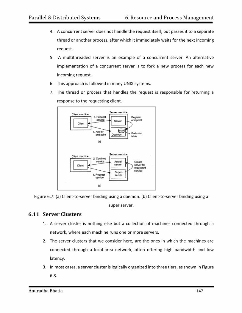
Parallel & Distributed Systems 6. Resource and Process Management
Anuradha Bhatia 147
4. A concurrent server does not handle the request itself, but passes it to a separate
thread or another process, after which it immediately waits for the next incoming
request.
5. A multithreaded server is an example of a concurrent server. An alternative
implementation of a concurrent server is to fork a new process for each new
incoming request.
6. This approach is followed in many UNIX systems.
7. The thread or process that handles the request is responsible for returning a
response to the requesting client.
Figure 6.7: (a) Client-to-server binding using a daemon. (b) Client-to-server binding using a
super server.
6.11 Server Clusters
1. A server cluster is nothing else but a collection of machines connected through a
network, where each machine runs one or more servers.
2. The server clusters that we consider here, are the ones in which the machines are
connected through a local-area network, often offering high bandwidth and low
latency.
3. In most cases, a server cluster is logically organized into three tiers, as shown in Figure
6.8.
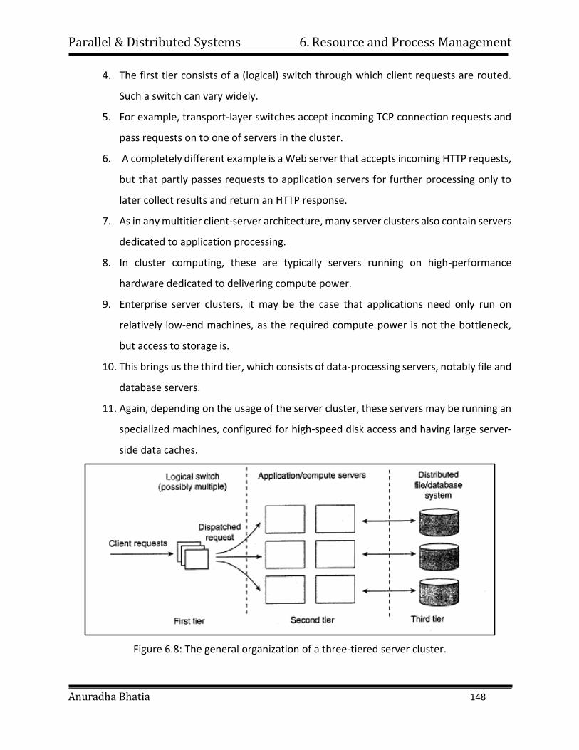
Parallel & Distributed Systems 6. Resource and Process Management
Anuradha Bhatia 148
4. The first tier consists of a (logical) switch through which client requests are routed.
Such a switch can vary widely.
5. For example, transport-layer switches accept incoming TCP connection requests and
pass requests on to one of servers in the cluster.
6. A completely different example is a Web server that accepts incoming HTTP requests,
but that partly passes requests to application servers for further processing only to
later collect results and return an HTTP response.
7. As in any multitier client-server architecture, many server clusters also contain servers
dedicated to application processing.
8. In cluster computing, these are typically servers running on high-performance
hardware dedicated to delivering compute power.
9. Enterprise server clusters, it may be the case that applications need only run on
relatively low-end machines, as the required compute power is not the bottleneck,
but access to storage is.
10. This brings us the third tier, which consists of data-processing servers, notably file and
database servers.
11. Again, depending on the usage of the server cluster, these servers may be running an
specialized machines, configured for high-speed disk access and having large server-
side data caches.
Figure 6.8: The general organization of a three-tiered server cluster.
Parallel & Distributed Systems 6. Resource and Process Management
Anuradha Bhatia 149
6.12 Code Migration
1. There are situations in which passing programs, sometimes even while they are being
executed, simplifies the design of a distributed system.
2. To start with by considering different approaches to code migration, followed by a
discussion on how to deal with the local resources that a migrating program uses.
3. Traditionally, code migration in distributed systems took place in the form of process
migration in which an entire process was moved from one machine to another.
4. Moving a running process to a different machine is a costly and intricate task, and
there had better be a good reason for doing so.
5. That reason has always been performance.
6. The basic idea is that overall system performance can be improved if processes are
moved from heavily-loaded to lightly-loaded machines.
7. Load is often expressed in terms of the CPU queue length or CPU utilization, but other
performance indicators are used as well.
8. Support for code migration can also help improve performance by exploiting
parallelism, but without the usual intricacies related to parallel programming.
9. A typical example is searching for information in the Web.
10. It is relatively simple to implement a search query in the form of a small mobile
program, called a mobile agent that moves from site to site.
11. By making several copies of such a program, and sending each off to different sites,
we may be able to achieve a linear speedup compared to using just a single program
instance.
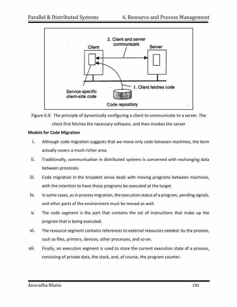
Parallel & Distributed Systems 6. Resource and Process Management
Anuradha Bhatia 150
Figure 6.9: The principle of dynamically configuring a client to communicate to a server. The
client first fetches the necessary software, and then invokes the server
Models for Code Migration
i. Although code migration suggests that we move only code between machines, the term
actually covers a much richer area.
ii. Traditionally, communication in distributed systems is concerned with exchanging data
between processes.
iii. Code migration in the broadest sense deals with moving programs between machines,
with the intention to have those programs be executed at the target.
iv. In some cases, as in process migration, the execution status of a program, pending signals,
and other parts of the environment must be moved as well.
v. The code segment is the part that contains the set of instructions that make up the
program that is being executed.
vi. The resource segment contains references to external resources needed. by the process,
such as files, printers, devices, other processes, and so on.
vii. Finally, an execution segment is used to store the current execution state of a process,
consisting of private data, the stack, and, of course, the program counter.
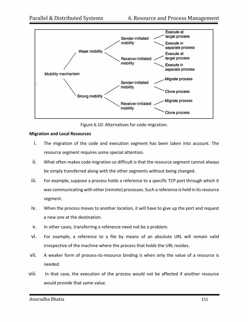
Parallel & Distributed Systems 6. Resource and Process Management
Anuradha Bhatia 151
Figure 6.10: Alternatives for code migration.
Migration and Local Resources
i. The migration of the code and execution segment has been taken into account. The
resource segment requires some special attention.
ii. What often makes code migration so difficult is that the resource segment cannot always
be simply transferred along with the other segments without being changed.
iii. For example, suppose a process holds a reference to a specific TCP port through which it
was communicating with other (remote) processes. Such a reference is held in its resource
segment.
iv. When the process moves to another location, it will have to give up the port and request
a new one at the destination.
v. In other cases, transferring a reference need not be a problem.
vi. For example, a reference to a file by means of an absolute URL will remain valid
irrespective of the machine where the process that holds the URL resides.
vii. A weaker form of process-to-resource binding is when only the value of a resource is
needed.
viii. In that case, the execution of the process would not be affected if another resource
would provide that same value.
Parallel & Distributed Systems 6. Resource and Process Management
Anuradha Bhatia 152
ix. A typical example of binding by value is when a program relies on standard libraries, such
as those for programming in C or Java.
x. Such libraries should always be locally available, but their exact location in the local file
system may differ between sites.
xi. Not the specific files, but their content is important for the proper execution of the
process.
Migration in Heterogeneous Systems
i. Migration in such systems requires that each platform is supported, that is, that the code
segment can be executed on each platform. Also, we need to ensure that the execution
segment can be properly represented at each platform.
ii. The problems coming from heterogeneity are in many respects the same as those of
portability.
iii. Not surprisingly, solutions are also very similar. For example, at the end of the 1970s, a
simple solution to alleviate many of the problems of porting Pascal to different machines
was to generate machine-independent intermediate code for an abstract virtual machine
(Barron, 1981).
iv. That machine, of course, would need to be implemented on many platforms, but it would
then allow Pascal programs to be run anywhere.
v. Although this simple idea was widely used for some years, it never really caught on as the
general solution to portability problems for other languages, notably C.
Three ways to handle migration
1. Pushing memory pages to the new machine and resending the ones that are later
modified during the migration process.
2. Stopping the current virtual machine; migrate memory, and start the new virtual
machine.
3. Letting the new virtual machine pull in new pages as needed, that is,let processes start
on the new virtual machine immediately and copy memory pages on demand.
Parallel & Distributed Systems
Anuradha Bhatia
7. Synchronization CONTENTS
7.1 Clock Synchronization, Logical Clocks, Election Algorithms, Mutual
Exclusion, Distributed Mutual Exclusion-Classification of mutual
Exclusion Algorithm, Requirements of Mutual Exclusion Algorithms,
Performance measure, Non Token based Algorithms: Lamport Algorithm,
Ricart–Agrawala’s Algorithm, Maekawa’s Algorithm.
7.2 Token Based Algorithms: Suzuki-Kasami’s Broardcast Algorithms,
Singhal’s Heurastic Algorithm, Raymond’s Tree based Algorithm,
Comparative Performance Analysis.
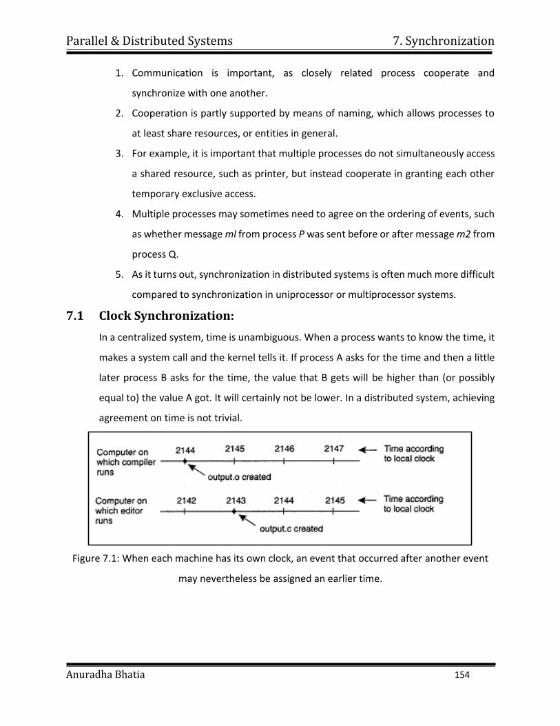
Parallel & Distributed Systems 7. Synchronization
Anuradha Bhatia 154
1. Communication is important, as closely related process cooperate and
synchronize with one another.
2. Cooperation is partly supported by means of naming, which allows processes to
at least share resources, or entities in general.
3. For example, it is important that multiple processes do not simultaneously access
a shared resource, such as printer, but instead cooperate in granting each other
temporary exclusive access.
4. Multiple processes may sometimes need to agree on the ordering of events, such
as whether message ml from process P was sent before or after message m2 from
process Q.
5. As it turns out, synchronization in distributed systems is often much more difficult
compared to synchronization in uniprocessor or multiprocessor systems.
7.1 Clock Synchronization:
In a centralized system, time is unambiguous. When a process wants to know the time, it
makes a system call and the kernel tells it. If process A asks for the time and then a little
later process B asks for the time, the value that B gets will be higher than (or possibly
equal to) the value A got. It will certainly not be lower. In a distributed system, achieving
agreement on time is not trivial.
Figure 7.1: When each machine has its own clock, an event that occurred after another event
may nevertheless be assigned an earlier time.
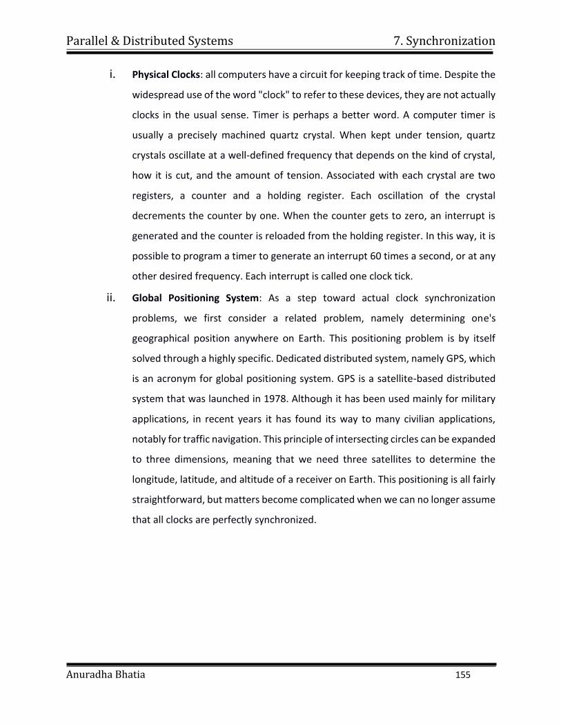
Parallel & Distributed Systems 7. Synchronization
Anuradha Bhatia 155
i. Physical Clocks: all computers have a circuit for keeping track of time. Despite the
widespread use of the word "clock" to refer to these devices, they are not actually
clocks in the usual sense. Timer is perhaps a better word. A computer timer is
usually a precisely machined quartz crystal. When kept under tension, quartz
crystals oscillate at a well-defined frequency that depends on the kind of crystal,
how it is cut, and the amount of tension. Associated with each crystal are two
registers, a counter and a holding register. Each oscillation of the crystal
decrements the counter by one. When the counter gets to zero, an interrupt is
generated and the counter is reloaded from the holding register. In this way, it is
possible to program a timer to generate an interrupt 60 times a second, or at any
other desired frequency. Each interrupt is called one clock tick.
ii. Global Positioning System: As a step toward actual clock synchronization
problems, we first consider a related problem, namely determining one's
geographical position anywhere on Earth. This positioning problem is by itself
solved through a highly specific. Dedicated distributed system, namely GPS, which
is an acronym for global positioning system. GPS is a satellite-based distributed
system that was launched in 1978. Although it has been used mainly for military
applications, in recent years it has found its way to many civilian applications,
notably for traffic navigation. This principle of intersecting circles can be expanded
to three dimensions, meaning that we need three satellites to determine the
longitude, latitude, and altitude of a receiver on Earth. This positioning is all fairly
straightforward, but matters become complicated when we can no longer assume
that all clocks are perfectly synchronized.
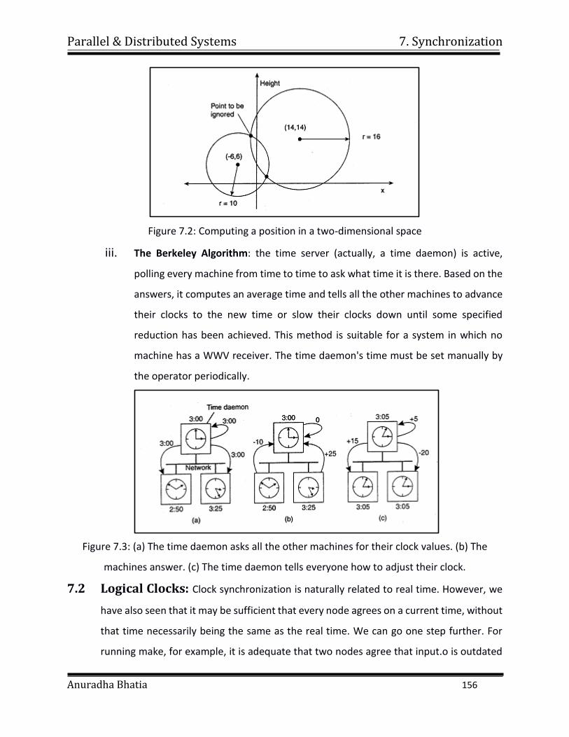
Parallel & Distributed Systems 7. Synchronization
Anuradha Bhatia 156
Figure 7.2: Computing a position in a two-dimensional space
iii. The Berkeley Algorithm: the time server (actually, a time daemon) is active,
polling every machine from time to time to ask what time it is there. Based on the
answers, it computes an average time and tells all the other machines to advance
their clocks to the new time or slow their clocks down until some specified
reduction has been achieved. This method is suitable for a system in which no
machine has a WWV receiver. The time daemon's time must be set manually by
the operator periodically.
Figure 7.3: (a) The time daemon asks all the other machines for their clock values. (b) The
machines answer. (c) The time daemon tells everyone how to adjust their clock.
7.2 Logical Clocks: Clock synchronization is naturally related to real time. However, we
have also seen that it may be sufficient that every node agrees on a current time, without
that time necessarily being the same as the real time. We can go one step further. For
running make, for example, it is adequate that two nodes agree that input.o is outdated
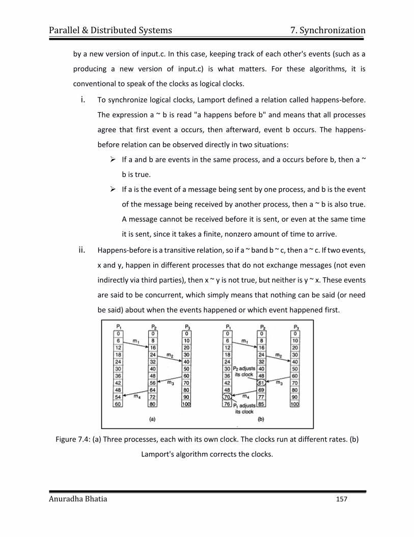
Parallel & Distributed Systems 7. Synchronization
Anuradha Bhatia 157
by a new version of input.c. In this case, keeping track of each other's events (such as a
producing a new version of input.c) is what matters. For these algorithms, it is
conventional to speak of the clocks as logical clocks.
i. To synchronize logical clocks, Lamport defined a relation called happens-before.
The expression a ~ b is read "a happens before b" and means that all processes
agree that first event a occurs, then afterward, event b occurs. The happens-
before relation can be observed directly in two situations:
If a and b are events in the same process, and a occurs before b, then a ~
b is true.
If a is the event of a message being sent by one process, and b is the event
of the message being received by another process, then a ~ b is also true.
A message cannot be received before it is sent, or even at the same time
it is sent, since it takes a finite, nonzero amount of time to arrive.
ii. Happens-before is a transitive relation, so if a ~ band b ~ c, then a ~ c. If two events,
x and y, happen in different processes that do not exchange messages (not even
indirectly via third parties), then x ~ y is not true, but neither is y ~ x. These events
are said to be concurrent, which simply means that nothing can be said (or need
be said) about when the events happened or which event happened first.
Figure 7.4: (a) Three processes, each with its own clock. The clocks run at different rates. (b)
Lamport's algorithm corrects the clocks.
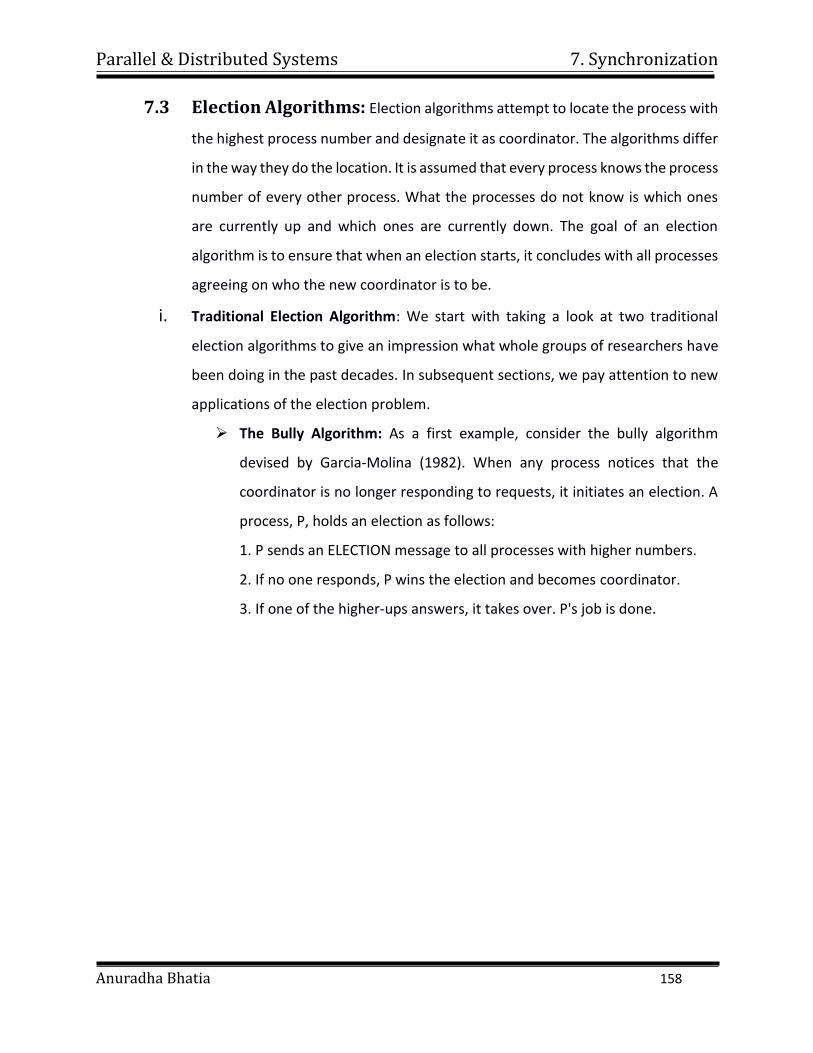
Parallel & Distributed Systems 7. Synchronization
Anuradha Bhatia 158
7.3 Election Algorithms: Election algorithms attempt to locate the process with
the highest process number and designate it as coordinator. The algorithms differ
in the way they do the location. It is assumed that every process knows the process
number of every other process. What the processes do not know is which ones
are currently up and which ones are currently down. The goal of an election
algorithm is to ensure that when an election starts, it concludes with all processes
agreeing on who the new coordinator is to be.
i. Traditional Election Algorithm: We start with taking a look at two traditional
election algorithms to give an impression what whole groups of researchers have
been doing in the past decades. In subsequent sections, we pay attention to new
applications of the election problem.
The Bully Algorithm: As a first example, consider the bully algorithm
devised by Garcia-Molina (1982). When any process notices that the
coordinator is no longer responding to requests, it initiates an election. A
process, P, holds an election as follows:
1. P sends an ELECTION message to all processes with higher numbers.
2. If no one responds, P wins the election and becomes coordinator.
3. If one of the higher-ups answers, it takes over. P's job is done.
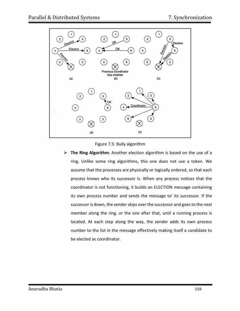
Parallel & Distributed Systems 7. Synchronization
Anuradha Bhatia 159
Figure 7.5: Bully algorithm
The Ring Algorithm: Another election algorithm is based on the use of a
ring. Unlike some ring algorithms, this one does not use a token. We
assume that the processes are physically or logically ordered, so that each
process knows who its successor is. When any process notices that the
coordinator is not functioning, it builds an ELECTION message containing
its own process number and sends the message to' its successor. If the
successor is down, the sender skips over the successor and goes to the next
member along the ring. or the one after that, until a running process is
located. At each step along the way, the sender adds its own process
number to the list in the message effectively making itself a candidate to
be elected as coordinator.
Parallel & Distributed Systems 7. Synchronization
Anuradha Bhatia 160
7.4 Mutual Exclusion
1. The problem of mutual exclusion frequently arises in distributed systems
whenever concurrent access to shared resources by several sites is involved.
2. For correctness, it is necessary that the shared resource be accessed by a single
site (or process) at a time.
3. A typical example is directory management, where an update to a directory must
be done atomically because if updates and reads to a directory proceed
concurrently, reads may obtain inconsistent information.
4. If an entry contains several fields, a read operation may read some fields before
the update and some after the update.
7.5 Distributed Mutual Exclusion
1. The problem of mutual exclusion in a single-computer system, where shared
memory exists.
2. In single-computer systems, the status of a shared resource and the status of users
is readily available in the shared memory, and solutions to the mutual exclusion
problem can be easily implemented using shared variables (e.g., semaphores).
3. In distributed systems, both the shared resources and the users may be
distributed and shared memory does not exist.
4. Consequently, approaches based on shared variables are not applicable to
distributed systems and approaches based on message passing must be used.
5. The problem of mutual exclusion becomes much more complex in distributed
systems (as compared to single-computer systems) because of the lack of both
shared memory and a common physical clock and because of unpredictable
message delays.
6. Owing to these factors, it is virtually impossible for a site in a distributed system
to have current and complete knowledge of the state of the system.
Parallel & Distributed Systems 7. Synchronization
Anuradha Bhatia 161
7.6 Classification of mutual Exclusion Algorithm
1. The problem of mutual exclusion has received considerable attention and several
algorithms to achieve mutual exclusion in distributed systems have been
proposed.
2. They tend to differ in their communication topology (e.g., tree, ring, and any
arbitrary graph) and in the amount of information maintained by each site about
other sites.
3. These algorithms can be grouped into two classes. The algorithms in the first class
are no token-based.
4. These algorithms require two or more successive rounds of message exchanges
among the sites.
5. These algorithms are assertion based because a site can enter its critical section
(CS) when an assertion defined on its local variables becomes true.
6. Mutual exclusion is enforced because the assertion becomes true only at one site
at any given time.
7. The algorithms in the second class are token-based, in these algorithms, a unique
token (also known as the PRIVILEGE message) is shared among the sites.
8. A site is allowed to enter its CS if it possesses the token and it continues to hold
the token until the execution of the CS is over.
9. These algorithms essentially differ in the way a site carries out the search for the
token.
7.7 Requirements of Mutual Exclusion Algorithms
The primary objective of a mutual exclusion algorithm is to maintain mutual exclusion;
that is, to guarantee that only one request accesses the es at a time. In addition, the
following characteristics are considered important in a mutual exclusion algorithm:
i. Freedom from Deadlocks. Two or more sites should not endlessly wait for
messages that will never arrive.
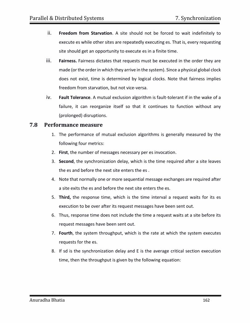
Parallel & Distributed Systems 7. Synchronization
Anuradha Bhatia 162
ii. Freedom from Starvation. A site should not be forced to wait indefinitely to
execute es while other sites are repeatedly executing es. That is, every requesting
site should get an opportunity to execute es in a finite time.
iii. Fairness. Fairness dictates that requests must be executed in the order they are
made (or the order in which they arrive in the system). Since a physical global clock
does not exist, time is determined by logical clocks. Note that fairness implies
freedom from starvation, but not vice-versa.
iv. Fault Tolerance. A mutual exclusion algorithm is fault-tolerant if in the wake of a
failure, it can reorganize itself so that it continues to function without any
(prolonged) disruptions.
7.8 Performance measure
1. The performance of mutual exclusion algorithms is generally measured by the
following four metrics:
2. First, the number of messages necessary per es invocation.
3. Second, the synchronization delay, which is the time required after a site leaves
the es and before the next site enters the es .
4. Note that normally one or more sequential message exchanges are required after
a site exits the es and before the next site enters the es.
5. Third, the response time, which is the time interval a request waits for its es
execution to be over after its request messages have been sent out.
6. Thus, response time does not include the time a request waits at a site before its
request messages have been sent out.
7. Fourth, the system throughput, which is the rate at which the system executes
requests for the es.
8. If sd is the synchronization delay and E is the average critical section execution
time, then the throughput is given by the following equation:
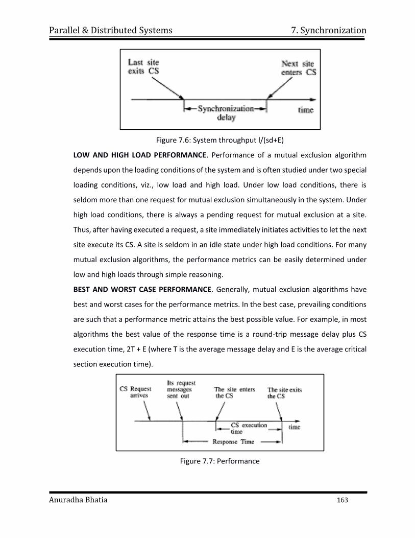
Parallel & Distributed Systems 7. Synchronization
Anuradha Bhatia 163
Figure 7.6: System throughput l/(sd+E)
LOW AND HIGH LOAD PERFORMANCE. Performance of a mutual exclusion algorithm
depends upon the loading conditions of the system and is often studied under two special
loading conditions, viz., low load and high load. Under low load conditions, there is
seldom more than one request for mutual exclusion simultaneously in the system. Under
high load conditions, there is always a pending request for mutual exclusion at a site.
Thus, after having executed a request, a site immediately initiates activities to let the next
site execute its CS. A site is seldom in an idle state under high load conditions. For many
mutual exclusion algorithms, the performance metrics can be easily determined under
low and high loads through simple reasoning.
BEST AND WORST CASE PERFORMANCE. Generally, mutual exclusion algorithms have
best and worst cases for the performance metrics. In the best case, prevailing conditions
are such that a performance metric attains the best possible value. For example, in most
algorithms the best value of the response time is a round-trip message delay plus CS
execution time, 2T + E (where T is the average message delay and E is the average critical
section execution time).
Figure 7.7: Performance
Parallel & Distributed Systems 7. Synchronization
Anuradha Bhatia 164
7.9 Non Token based Algorithms:
1. In non-taken-based mutual exclusion algorithms, a site communicates with a set
of other sites to arbitrate who should execute the CS next. For a site Si.
2. Request set Ri contains ids of all those sites from which site Si must acquire
permission before entering the CS.
3. Non-token-based mutual exclusion algorithms which are good representatives of
this class.
4. Non-token-based mutual exclusion algorithms use timestamps to order requests
for the CS and to resolve conflicts between simultaneous requests for the CS.
5. In all these algorithms, logical clocks are maintained and updated according to
Lamport's scheme [9]. Each request for the CS gets a timestamp, and smaller
timestamp requests have priority over larger timestamp requests.
i. Lamport Algorithm
Lamport was the first to give a distributed mutual exclusion algorithm as an
illustration of his clock synchronization scheme [9]. In Lamport's algorithm,
. I : 1 <= I <= N :: Ri = {S1,S2,…..,S3}
Every site Si keeps a queue, request.queuei which contains mutual exclusion
requests ordered by their timestamps. This algorithm requires messages to be
delivered in the FIFO order between every pair of sites.
The Algorithm
Requesting the critical section:
1. When a site Si wants to enter the CS, it sends a REQUEST(tsi, i) message to
all the sites in its request set Ri and places the request on
reques.queuei.((tsi, i) is the timestamp of the request.)
2. When a site H j receives the REQUEST(t8i, i) message from site Si, it retums
a timestamped REPLY message to and places site Si 's request on
reques.queue}.
Executing the critical section. Site Hi enters the CS when the two following
conditions hold:
Parallel & Distributed Systems 7. Synchronization
Anuradha Bhatia 165
[L1:] Hi has received a message with timestamp larger than (t8i, i) from all other
sites.
[L2:] Hi'S request is at the top of requesLqueuei.
Releasing the critical section.
1. Site Si, upon exiting the CS, removes its request from the top of its request
queue and sends a timestamped RELEASE message to all the sites in its
request set.
2. When a site S} receives a RELEASE message from site Hi, it removes Si'S
request from its request queue.
When a site removes a request from its request queue, its own request may come
at the top of the queue, enabling it to enter the CS. The algorithm executes CS
requests in the increasing order of timestamps.
ii. Ricart–Agrawala’s Algorithm
The Ricart-Agrawala algorithm [16] is an optimization of Lamport's algorithm that
dispenses with RELEASE messages by cleverly merging them with REPLY messages. In this
algorithm also, I : 1 <= I <= N :: Ri = {S1,S2,…..,SN}
The Algorithm
Requesting the critical section.
1. When a site Si wants to enter the CS, it sends a timestamped REQUEST message
to all the sites in its request set.
2. When site Sj receives a REQUEST message from site Si, it sends a REPLY message
to site Si if site Sj is neither requesting nor executing the CS or if site Sj is requesting
and Si'S request's timestamp is smaller than site S/s own request's timestamp. The
request is deferred otherwise.
Executing the critical section
3. Site Si enters the CS after it has received REPLY messages from all the sites in its
request set.
Releasing the critical section
4. When site Si exits the CS, it sends REPLY messages to all the deferred requests.
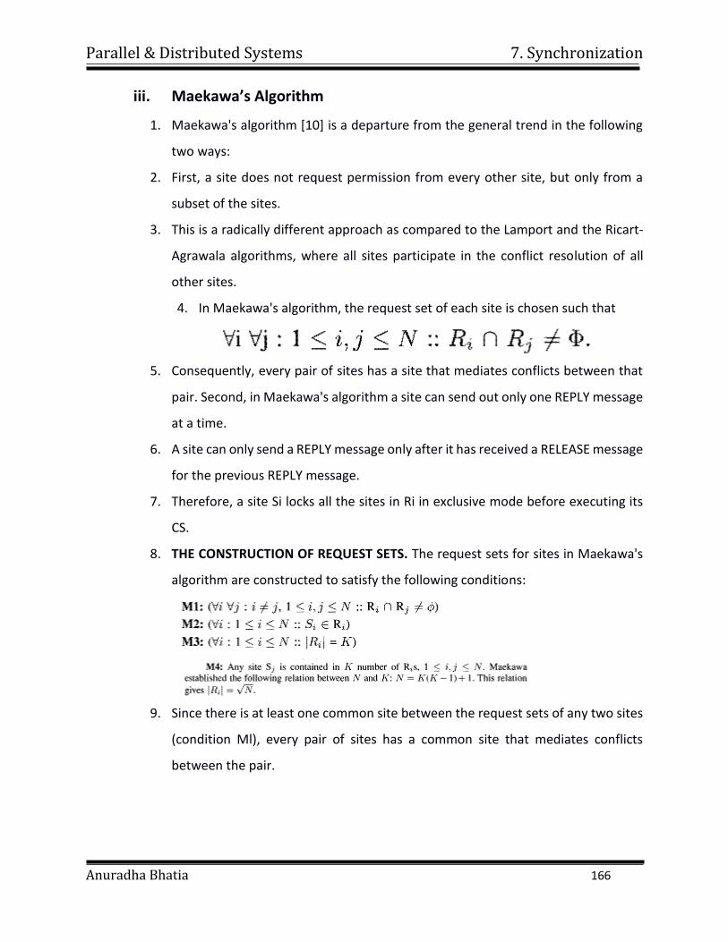
Parallel & Distributed Systems 7. Synchronization
Anuradha Bhatia 166
iii. Maekawa’s Algorithm
1. Maekawa's algorithm [10] is a departure from the general trend in the following
two ways:
2. First, a site does not request permission from every other site, but only from a
subset of the sites.
3. This is a radically different approach as compared to the Lamport and the Ricart-
Agrawala algorithms, where all sites participate in the conflict resolution of all
other sites.
4. In Maekawa's algorithm, the request set of each site is chosen such that
5. Consequently, every pair of sites has a site that mediates conflicts between that
pair. Second, in Maekawa's algorithm a site can send out only one REPLY message
at a time.
6. A site can only send a REPLY message only after it has received a RELEASE message
for the previous REPLY message.
7. Therefore, a site Si locks all the sites in Ri in exclusive mode before executing its
CS.
8. THE CONSTRUCTION OF REQUEST SETS. The request sets for sites in Maekawa's
algorithm are constructed to satisfy the following conditions:
9. Since there is at least one common site between the request sets of any two sites
(condition Ml), every pair of sites has a common site that mediates conflicts
between the pair.
Parallel & Distributed Systems 7. Synchronization
Anuradha Bhatia 167
10. A site can have only one outstanding REPLY message at any time; that is, it grants
permission to an incoming request if it has not granted permission to some other
site. Therefore, mutual exclusion is guaranteed.
11. This algorithm requires the delivery of messages to be in the order they are sent
between every pair of sites.
The Algorithm
Maekawa's algorithm works in the following manner:
Requesting the critical section.
i. A site Si requests access to the CS by sending REQUEST(i) messages to all
the sites in its request set Ri .
ii. When a site Sj receives the REQUEST(i) message, it sends a REPLY(j)
message to Si provided it hasn't sent a REPLY message to a site from the
time it received the last RELEASE message. Otherwise, it queues up the
REQUEST for later consideration.
Executing the critical section.
iii. Site Si accesses the CS only after receiving REPLY messages from all the
sites in Ri’
Releasing the critical section
iv. After the execution of the CS is over, site Si sends RELEASE(i) message to
all the sites in Ri.
v. When a site Sj receives a RELEASE(i) message from site Si, it sends a
REPLY message to the next site waiting in the queue and deletes that entry
from the queue. If the queue is empty, then the site updates its state to
reflect that the site has not sent out any REPLY message.
Parallel & Distributed Systems 7. Synchronization
Anuradha Bhatia 168
7.10 Token Based Algorithms
i. In token-based algorithms, a unique token is shared among all sites.
ii. A site is allowed to enter its CS if it possesses the token.
iii. Depending upon the way a site carries out its search for the token, there are
numerous token-based algorithms.
iv. Token-based algorithms use sequence numbers instead of timestamps. Every
request for the token contains a sequence number and the sequence numbers
of sites advance independently.
v. A site increments its sequence number counter every time it makes a request
for the token.
vi. A primary function of the sequence numbers is to distinguish between old and
current requests.
vii. Second, a correctness proof of token-based algorithms to ensure that mutual
exclusion is enforced is trivial because an algorithm guarantees mutual
exclusion so long as a site holds the token during the execution of the CS..
7.11 Suzuki-Kasami’s Broardcast Algorithms
1. In the Suzuki-Kasami's algorithm [21], if a site attempting to enter the CS does not
have the token, it broadcasts a REQUEST message for the token to all the other
sites.
2. A site that possesses the token sends it to the requesting site upon receiving its
REQUEST message.
3. If a site receives a REQUEST message when it is executing the CS, it sends the token
only after it has exited the CS.
4. A site holding the token can enter its CS repeatedly until it sends the token to
some other site.
5. The main design issues in this algorithm are:
Distinguishing outdated REQUEST messages from current REQUEST
messages
Parallel & Distributed Systems 7. Synchronization
Anuradha Bhatia 169
Determining which site has an outstanding request for the CS.
The Algorithm
Requesting the critical section
i. If the requesting site 5i does not have the token, then it increments its
sequence number, RNi[i], and sends a REQUEST(i, sn) message to all other
sites. (sn is the updated value of RNdi].)
ii. When a site 5 j receives this message, it sets RNj[i] to max(RNj[i], sn). If 5 j has
the idle token, then it sends the token to 5 i if RNj [i]=LN[i]+1.
Executing the critical section.
iii. Site 5i executes the CS when it has received the token.
Releasing the critical section. Having finished the execution of the CS, site 5 i takes the
following actions:
iv. It sets LN[i] element of the token array equal to RNdi].
v. For every site 5 j whose 10 is not in the token queue, it appends its 10 to the
token queue if RNi [j]=LN[j]+1.
vi. If token queue is nonempty after the above update, then it deletes the top site
ID from the queue and sends the token to the site indicated by the 10.
Thus, after having executed its CS, a site gives priority to other sites with outstanding
requests for the CS (over its pending requests for the CS). The Suzuki-Kasami algorithm is
not symmetric because a site retains the token even if it does not have a request for the
CS, which is contrary to the spirit of Ricart and Agrawala's definition of a symmetric
algorithm: "no site possesses the right to access its CS when it has not been requested.”
7.12 Singhal’s Heurastic Algorithm
1. In Singhal's token-based heuristic algorithm [20], each site maintains information
about the state of other sites in the system and uses it to select a set of sites that
are likely to have the token.
2. The site requests the token only from these sites, reducing the number of
messages required to execute the CS.
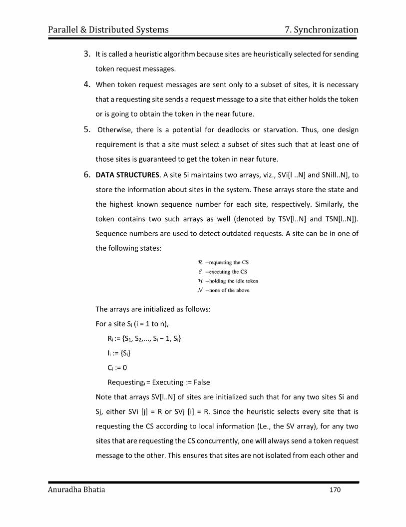
Parallel & Distributed Systems 7. Synchronization
Anuradha Bhatia 170
3. It is called a heuristic algorithm because sites are heuristically selected for sending
token request messages.
4. When token request messages are sent only to a subset of sites, it is necessary
that a requesting site sends a request message to a site that either holds the token
or is going to obtain the token in the near future.
5. Otherwise, there is a potential for deadlocks or starvation. Thus, one design
requirement is that a site must select a subset of sites such that at least one of
those sites is guaranteed to get the token in near future.
6. DATA STRUCTURES. A site Si maintains two arrays, viz., SVi[l ..N] and SNill..N], to
store the information about sites in the system. These arrays store the state and
the highest known sequence number for each site, respectively. Similarly, the
token contains two such arrays as well (denoted by TSV[l..N] and TSN[l..N]).
Sequence numbers are used to detect outdated requests. A site can be in one of
the following states:
The arrays are initialized as follows:
For a site Si (i = 1 to n),
Ri := {S1, S2,..., Si − 1, Si}
Ii := {Si}
Ci := 0
Requestingi = Executingi := False
Note that arrays SV[l..N] of sites are initialized such that for any two sites Si and
Sj, either SVi [j] = R or SVj [i] = R. Since the heuristic selects every site that is
requesting the CS according to local information (Le., the SV array), for any two
sites that are requesting the CS concurrently, one will always send a token request
message to the other. This ensures that sites are not isolated from each other and
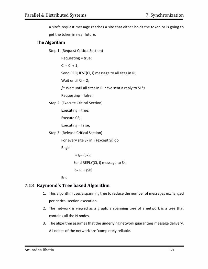
Parallel & Distributed Systems 7. Synchronization
Anuradha Bhatia 171
a site's request message reaches a site that either holds the token or is going to
get the token in near future.
The Algorithm
Step 1: (Request Critical Section)
Requesting = true;
Ci = Ci + 1;
Send REQUEST(Ci, i) message to all sites in Ri;
Wait until Ri = ∅;
/* Wait until all sites in Ri have sent a reply to Si */
Requesting = false;
Step 2: (Execute Critical Section)
Executing = true;
Execute CS;
Executing = false;
Step 3: (Release Critical Section)
For every site Sk in Ii (except Si) do
Begin
Ii= Ii – {Sk};
Send REPLY(Ci, i) message to Sk;
Ri= Ri + {Sk}
End
7.13 Raymond’s Tree based Algorithm
1. This algorithm uses a spanning tree to reduce the number of messages exchanged
per critical section execution.
2. The network is viewed as a graph, a spanning tree of a network is a tree that
contains all the N nodes.
3. The algorithm assumes that the underlying network guarantees message delivery.
All nodes of the network are ’completely reliable.
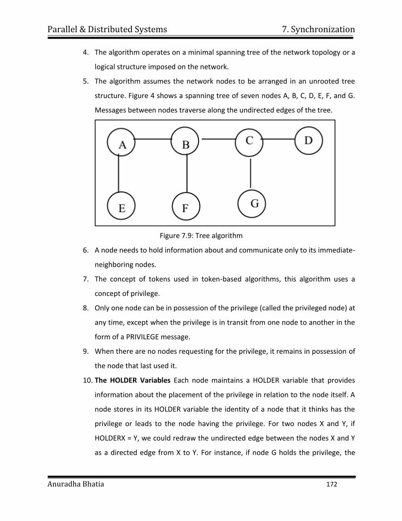
Parallel & Distributed Systems 7. Synchronization
Anuradha Bhatia 172
4. The algorithm operates on a minimal spanning tree of the network topology or a
logical structure imposed on the network.
5. The algorithm assumes the network nodes to be arranged in an unrooted tree
structure. Figure 4 shows a spanning tree of seven nodes A, B, C, D, E, F, and G.
Messages between nodes traverse along the undirected edges of the tree.
Figure 7.9: Tree algorithm
6. A node needs to hold information about and communicate only to its immediate-
neighboring nodes.
7. The concept of tokens used in token-based algorithms, this algorithm uses a
concept of privilege.
8. Only one node can be in possession of the privilege (called the privileged node) at
any time, except when the privilege is in transit from one node to another in the
form of a PRIVILEGE message.
9. When there are no nodes requesting for the privilege, it remains in possession of
the node that last used it.
10. The HOLDER Variables Each node maintains a HOLDER variable that provides
information about the placement of the privilege in relation to the node itself. A
node stores in its HOLDER variable the identity of a node that it thinks has the
privilege or leads to the node having the privilege. For two nodes X and Y, if
HOLDERX = Y, we could redraw the undirected edge between the nodes X and Y
as a directed edge from X to Y. For instance, if node G holds the privilege, the
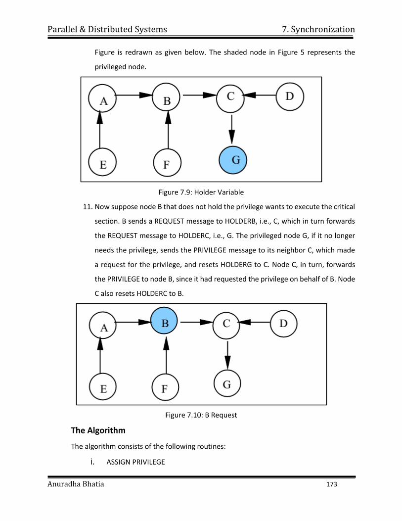
Parallel & Distributed Systems 7. Synchronization
Anuradha Bhatia 173
Figure is redrawn as given below. The shaded node in Figure 5 represents the
privileged node.
Figure 7.9: Holder Variable
11. Now suppose node B that does not hold the privilege wants to execute the critical
section. B sends a REQUEST message to HOLDERB, i.e., C, which in turn forwards
the REQUEST message to HOLDERC, i.e., G. The privileged node G, if it no longer
needs the privilege, sends the PRIVILEGE message to its neighbor C, which made
a request for the privilege, and resets HOLDERG to C. Node C, in turn, forwards
the PRIVILEGE to node B, since it had requested the privilege on behalf of B. Node
C also resets HOLDERC to B.
Figure 7.10: B Request
The Algorithm
The algorithm consists of the following routines:
i. ASSIGN PRIVILEGE
Parallel & Distributed Systems 7. Synchronization
Anuradha Bhatia 174
This is a routine sends a PRIVILEGE message. A privileged node sends a
PRIVILEGE message if
it holds the privilege but is not using it,
its REQUEST Q is not empty, and
The element at the head of its REQUEST Q is not “self.”
ii. MAKE REQUEST
This is a routine sends a REQUEST message. An unprivileged node sends a
REQUEST message if
it does not hold the privilege,
its REQUEST Q is not empty, i.e., it requires the privilege for itself, or
on behalf of one of its immediate neighboring nodes, and
it has not sent a REQUEST message already.
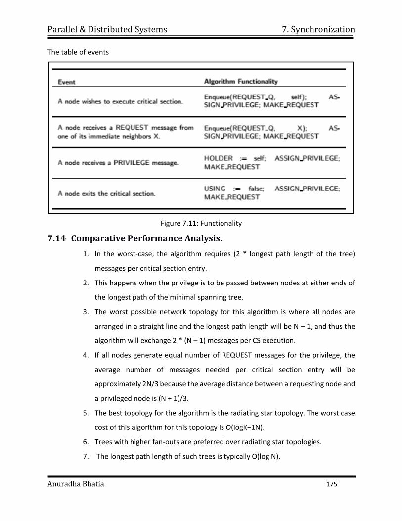
Parallel & Distributed Systems 7. Synchronization
Anuradha Bhatia 175
The table of events
Figure 7.11: Functionality
7.14 Comparative Performance Analysis.
1. In the worst-case, the algorithm requires (2 * longest path length of the tree)
messages per critical section entry.
2. This happens when the privilege is to be passed between nodes at either ends of
the longest path of the minimal spanning tree.
3. The worst possible network topology for this algorithm is where all nodes are
arranged in a straight line and the longest path length will be N – 1, and thus the
algorithm will exchange 2 * (N – 1) messages per CS execution.
4. If all nodes generate equal number of REQUEST messages for the privilege, the
average number of messages needed per critical section entry will be
approximately 2N/3 because the average distance between a requesting node and
a privileged node is (N + 1)/3.
5. The best topology for the algorithm is the radiating star topology. The worst case
cost of this algorithm for this topology is O(logK−1N).
6. Trees with higher fan-outs are preferred over radiating star topologies.
7. The longest path length of such trees is typically O(log N).
Parallel & Distributed Systems 7. Synchronization
Anuradha Bhatia 176
8. Thus, on an average, this algorithm involves the exchange of O(log N) messages
per critical section execution. Under heavy load, the algorithm exhibits an
interesting property:
9. “As the number of nodes requesting for the privilege increases, the number of
messages exchanged per critical section entry decreases.” In heavy load, the
algorithm requires exchange of only four messages per CS execution.
Parallel & Distributed Systems
Anuradha Bhatia
8. Consistency and Replication
CONTENTS
8.1 Introduction, Data-Centric and Client-Centric Consistency Models, Replica
Management.
8.2 Introduction, good features of DFS, File models, File Accessing models,
File-Caching Schemes, File Replication, Network File System(NFS),
Andrew File System(AFS), Hadoop Distributed File System and Map
Reduce.
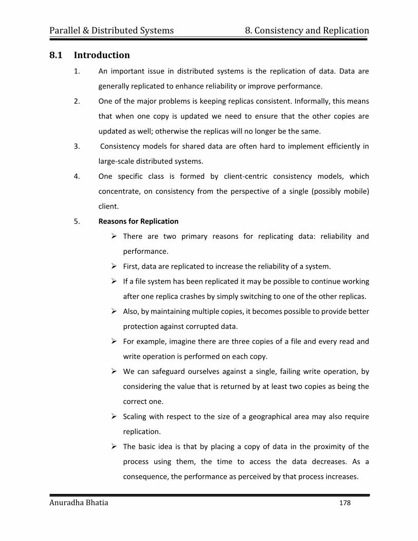
Parallel & Distributed Systems 8. Consistency and Replication
Anuradha Bhatia 178
8.1 Introduction
1. An important issue in distributed systems is the replication of data. Data are
generally replicated to enhance reliability or improve performance.
2. One of the major problems is keeping replicas consistent. Informally, this means
that when one copy is updated we need to ensure that the other copies are
updated as well; otherwise the replicas will no longer be the same.
3. Consistency models for shared data are often hard to implement efficiently in
large-scale distributed systems.
4. One specific class is formed by client-centric consistency models, which
concentrate, on consistency from the perspective of a single (possibly mobile)
client.
5. Reasons for Replication
There are two primary reasons for replicating data: reliability and
performance.
First, data are replicated to increase the reliability of a system.
If a file system has been replicated it may be possible to continue working
after one replica crashes by simply switching to one of the other replicas.
Also, by maintaining multiple copies, it becomes possible to provide better
protection against corrupted data.
For example, imagine there are three copies of a file and every read and
write operation is performed on each copy.
We can safeguard ourselves against a single, failing write operation, by
considering the value that is returned by at least two copies as being the
correct one.
Scaling with respect to the size of a geographical area may also require
replication.
The basic idea is that by placing a copy of data in the proximity of the
process using them, the time to access the data decreases. As a
consequence, the performance as perceived by that process increases.
Parallel & Distributed Systems 8. Consistency and Replication
Anuradha Bhatia 179
This example also illustrates that the benefits of replication for
performance may be hard to evaluate.
Although a client process may perceive better performance, it may also be
the case that more network bandwidth is now consumed keeping all
replicas up to date.
6. Replication as Scaling Technique
Replication and caching for performance are widely applied as scaling
techniques. Scalability issues generally appear in the form of performance
problems.
Placing copies of data close to the processes using them can improve
performance through reduction of access time and thus solve scalability
problems.
A possible trade-off that needs to be made is that keeping copies up to
date may require more network bandwidth.
Consider a process P that accesses a local replica N times per second,
whereas the replica itself is updated M times per second.
Assume that an update completely refreshes the previous version of the
local replica.
If N «M, that is, the access-to-update ratio is very low, we have the
situation where many updated versions of the local replica will never be
accessed by P, rendering the network communication for those versions
useless.
It may have been better not to install a local replica close to P, or to apply
a different strategy for updating the replica.
Parallel & Distributed Systems 8. Consistency and Replication
Anuradha Bhatia 180
8.2 Data-Centric and Client-Centric Consistency Models
1. Data Centric Consistency Model
A data store may be physically distributed across multiple machines. In
particular, each process that can access data from the store is assumed
to have a local (or nearby) copy available of the entire store.
Write operations are propagated to the other copies, as shown in
Figure.
A data operation is classified as a write operation when it changes the
data, and is otherwise classified as a read operation.
Figure 8.1: Data Centric Model
A consistency model is essentially a contract between processes and
the data store. It says that if processes agree to obey certain. Rules, the
store promises to work correctly.
Normally, a process that performs a read operation on a data item,
expects the operation to return a value that shows the results of the last
write operation on that data.
In the absence of a global clock, it is difficult to define precisely which
write operation is the last one. As an alternative, we need to provide
other definitions, leading to a range of consistency models.
Each model effectively restricts the values that a read operation on a
data item can return.
Parallel & Distributed Systems 8. Consistency and Replication
Anuradha Bhatia 181
As is to be expected, the ones with major restrictions are easy to use,
for example when developing applications, whereas those with minor
restrictions are sometimes difficult.
The tradeoff is, of course, that the easy-to-use models do not perform
nearly as well as the difficult ones.
2. Client-Centric Consistency Models
The consistency models described in the previous section aim at
providing a system wide consistent view on a data store.
An important assumption is that concurrent processes may be
simultaneously updating the data store, and that it is necessary to
provide consistency in the face of such concurrency.
For example, in the case of object-based entry consistency, the data
store guarantees that when an object is called, the calling process is
provided with a copy of the object that reflects all changes to the object
that have been made so far, possibly by other processes.
During the call, it is also guaranteed that no other process can interfere
that is, mutual exclusive access is provided to the calling process.
Eventual Consistency There are many examples in which concurrency
appears only in a restricted form. For example, in many database
systems, most processes hardly ever perform update operations; they
mostly read data from the database. Only one, or very few processes
perform update operations. The question then is how fast updates
should be made available to only reading processes.
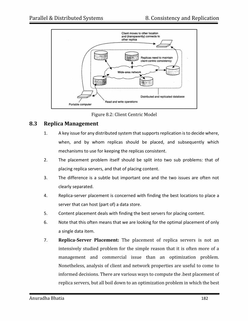
Parallel & Distributed Systems 8. Consistency and Replication
Anuradha Bhatia 182
Figure 8.2: Client Centric Model
8.3 Replica Management
1. A key issue for any distributed system that supports replication is to decide where,
when, and by whom replicas should be placed, and subsequently which
mechanisms to use for keeping the replicas consistent.
2. The placement problem itself should be split into two sub problems: that of
placing replica servers, and that of placing content.
3. The difference is a subtle but important one and the two issues are often not
clearly separated.
4. Replica-server placement is concerned with finding the best locations to place a
server that can host (part of) a data store.
5. Content placement deals with finding the best servers for placing content.
6. Note that this often means that we are looking for the optimal placement of only
a single data item.
7. Replica-Server Placement: The placement of replica servers is not an
intensively studied problem for the simple reason that it is often more of a
management and commercial issue than an optimization problem.
Nonetheless, analysis of client and network properties are useful to come to
informed decisions. There are various ways to compute the .best placement of
replica servers, but all boil down to an optimization problem in which the best
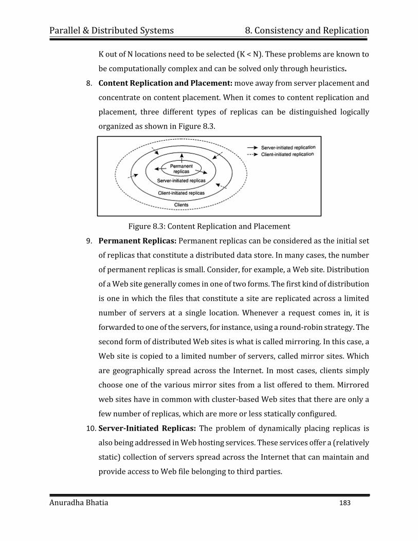
Parallel & Distributed Systems 8. Consistency and Replication
Anuradha Bhatia 183
K out of N locations need to be selected (K < N). These problems are known to
be computationally complex and can be solved only through heuristics.
8. Content Replication and Placement: move away from server placement and
concentrate on content placement. When it comes to content replication and
placement, three different types of replicas can be distinguished logically
organized as shown in Figure 8.3.
Figure 8.3: Content Replication and Placement
9. Permanent Replicas: Permanent replicas can be considered as the initial set
of replicas that constitute a distributed data store. In many cases, the number
of permanent replicas is small. Consider, for example, a Web site. Distribution
of a Web site generally comes in one of two forms. The first kind of distribution
is one in which the files that constitute a site are replicated across a limited
number of servers at a single location. Whenever a request comes in, it is
forwarded to one of the servers, for instance, using a round-robin strategy. The
second form of distributed Web sites is what is called mirroring. In this case, a
Web site is copied to a limited number of servers, called mirror sites. Which
are geographically spread across the Internet. In most cases, clients simply
choose one of the various mirror sites from a list offered to them. Mirrored
web sites have in common with cluster-based Web sites that there are only a
few number of replicas, which are more or less statically configured.
10. Server-Initiated Replicas: The problem of dynamically placing replicas is
also being addressed in Web hosting services. These services offer a (relatively
static) collection of servers spread across the Internet that can maintain and
provide access to Web file belonging to third parties.
Parallel & Distributed Systems 8. Consistency and Replication
Anuradha Bhatia 184
8.4 Introduction, good features of DFS
1. A Distributed File System (DFS) enables programs to store and access remote files
exactly as they do local ones, allowing users to access files from any computer on
a network. This is an area of active research interest today.
2. The resources on a particular machine are local to itself. Resources on other
machines are remote.
3. A file system provides a service for clients. The server interface is the normal set
of file operations: create, read, etc. on files.
4. Key Features
Data sharing of multiple users.
User mobility
Location transparency
Location independence
Backups and System Monitoring
8.5 File models
1. File Transfer Protocol(FTP)
Connect to a remote machine and interactively send or fetch an arbitrary
file.
User connecting to an FTP server specifies an account and password.
Superseded by HTTP for file transfer.
2. Sun's Network File System.
One of the most popular and widespread distributed file system in use today
since its introduction in 1985.
Motivated by wanting to extend a UNIX file system to a distributed
environment. But, further extended to other OS as well.
Design is transparent. Any computer can be a server, exporting some of its
files, and a client, accessing files on other machines.
High performance: try to make remote access as comparable to local access
through caching and readahead.
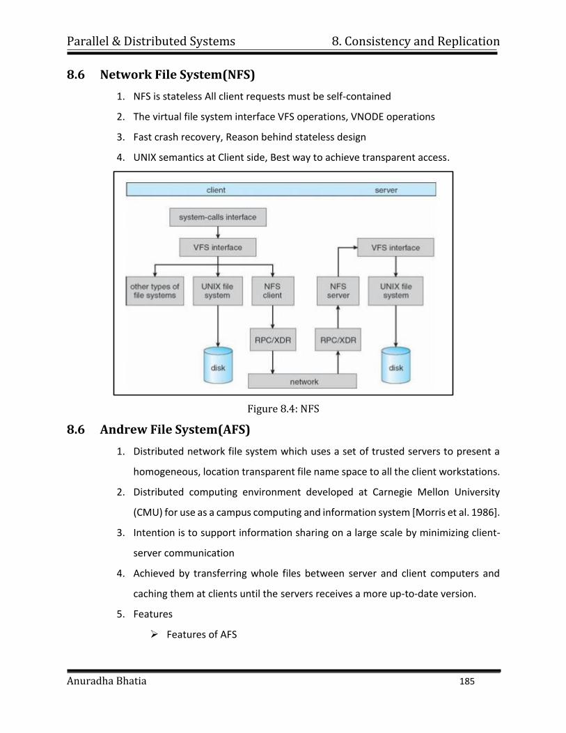
Parallel & Distributed Systems 8. Consistency and Replication
Anuradha Bhatia 185
8.6 Network File System(NFS)
1. NFS is stateless All client requests must be self-contained
2. The virtual file system interface VFS operations, VNODE operations
3. Fast crash recovery, Reason behind stateless design
4. UNIX semantics at Client side, Best way to achieve transparent access.
Figure 8.4: NFS
8.6 Andrew File System(AFS)
1. Distributed network file system which uses a set of trusted servers to present a
homogeneous, location transparent file name space to all the client workstations.
2. Distributed computing environment developed at Carnegie Mellon University
(CMU) for use as a campus computing and information system [Morris et al. 1986].
3. Intention is to support information sharing on a large scale by minimizing client-
server communication
4. Achieved by transferring whole files between server and client computers and
caching them at clients until the servers receives a more up-to-date version.
5. Features
Features of AFS
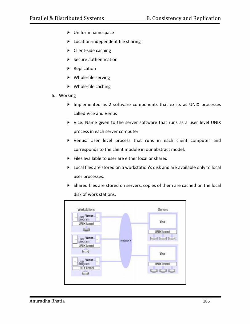
Parallel & Distributed Systems 8. Consistency and Replication
Anuradha Bhatia 186
Uniform namespace
Location-independent file sharing
Client-side caching
Secure authentication
Replication
Whole-file serving
Whole-file caching
6. Working
Implemented as 2 software components that exists as UNIX processes
called Vice and Venus
Vice: Name given to the server software that runs as a user level UNIX
process in each server computer.
Venus: User level process that runs in each client computer and
corresponds to the client module in our abstract model.
Files available to user are either local or shared
Local files are stored on a workstation's disk and are available only to local
user processes.
Shared files are stored on servers, copies of them are cached on the local
disk of work stations.
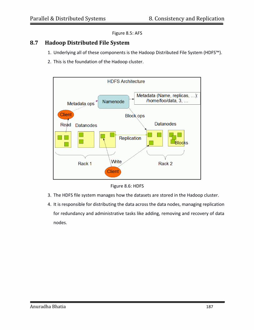
Parallel & Distributed Systems 8. Consistency and Replication
Anuradha Bhatia 187
Figure 8.5: AFS
8.7 Hadoop Distributed File System
1. Underlying all of these components is the Hadoop Distributed File System (HDFS™).
2. This is the foundation of the Hadoop cluster.
Figure 8.6: HDFS
3. The HDFS file system manages how the datasets are stored in the Hadoop cluster.
4. It is responsible for distributing the data across the data nodes, managing replication
for redundancy and administrative tasks like adding, removing and recovery of data
nodes.
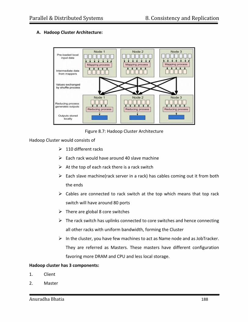
Parallel & Distributed Systems 8. Consistency and Replication
Anuradha Bhatia 188
A. Hadoop Cluster Architecture:
Figure 8.7: Hadoop Cluster Architecture
Hadoop Cluster would consists of
110 different racks
Each rack would have around 40 slave machine
At the top of each rack there is a rack switch
Each slave machine(rack server in a rack) has cables coming out it from both
the ends
Cables are connected to rack switch at the top which means that top rack
switch will have around 80 ports
There are global 8 core switches
The rack switch has uplinks connected to core switches and hence connecting
all other racks with uniform bandwidth, forming the Cluster
In the cluster, you have few machines to act as Name node and as JobTracker.
They are referred as Masters. These masters have different configuration
favoring more DRAM and CPU and less local storage.
Hadoop cluster has 3 components:
1. Client
2. Master
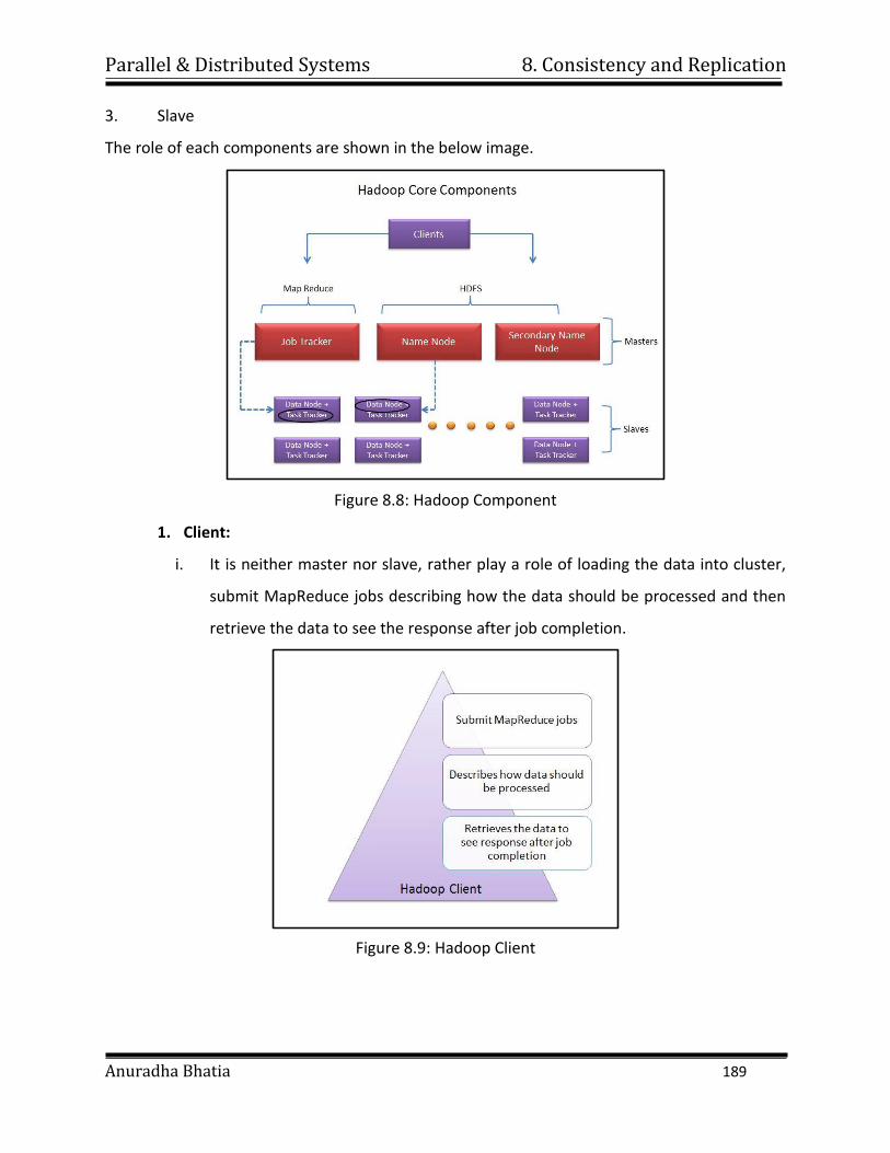
Parallel & Distributed Systems 8. Consistency and Replication
Anuradha Bhatia 189
3. Slave
The role of each components are shown in the below image.
Figure 8.8: Hadoop Component
1. Client:
i. It is neither master nor slave, rather play a role of loading the data into cluster,
submit MapReduce jobs describing how the data should be processed and then
retrieve the data to see the response after job completion.
Figure 8.9: Hadoop Client
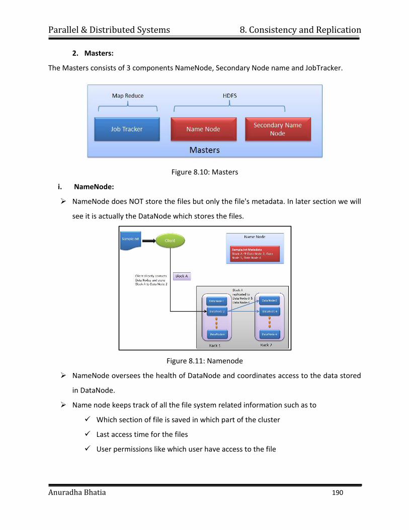
Parallel & Distributed Systems 8. Consistency and Replication
Anuradha Bhatia 190
2. Masters:
The Masters consists of 3 components NameNode, Secondary Node name and JobTracker.
Figure 8.10: Masters
i. NameNode:
NameNode does NOT store the files but only the file's metadata. In later section we will
see it is actually the DataNode which stores the files.
Figure 8.11: Namenode
NameNode oversees the health of DataNode and coordinates access to the data stored
in DataNode.
Name node keeps track of all the file system related information such as to
Which section of file is saved in which part of the cluster
Last access time for the files
User permissions like which user have access to the file
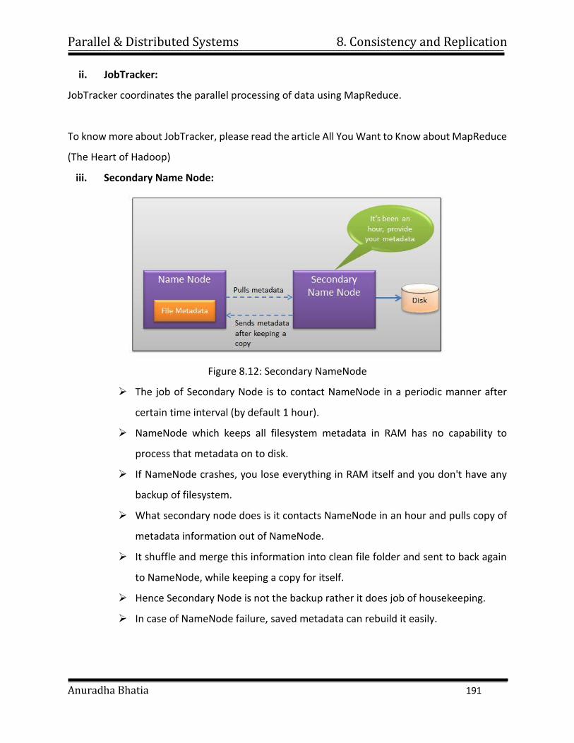
Parallel & Distributed Systems 8. Consistency and Replication
Anuradha Bhatia 191
ii. JobTracker:
JobTracker coordinates the parallel processing of data using MapReduce.
To know more about JobTracker, please read the article All You Want to Know about MapReduce
(The Heart of Hadoop)
iii. Secondary Name Node:
Figure 8.12: Secondary NameNode
The job of Secondary Node is to contact NameNode in a periodic manner after
certain time interval (by default 1 hour).
NameNode which keeps all filesystem metadata in RAM has no capability to
process that metadata on to disk.
If NameNode crashes, you lose everything in RAM itself and you don't have any
backup of filesystem.
What secondary node does is it contacts NameNode in an hour and pulls copy of
metadata information out of NameNode.
It shuffle and merge this information into clean file folder and sent to back again
to NameNode, while keeping a copy for itself.
Hence Secondary Node is not the backup rather it does job of housekeeping.
In case of NameNode failure, saved metadata can rebuild it easily.
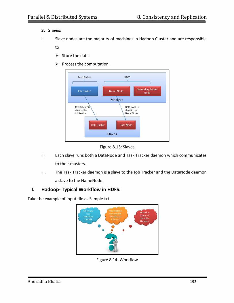
Parallel & Distributed Systems 8. Consistency and Replication
Anuradha Bhatia 192
3. Slaves:
i. Slave nodes are the majority of machines in Hadoop Cluster and are responsible
to
Store the data
Process the computation
Figure 8.13: Slaves
ii. Each slave runs both a DataNode and Task Tracker daemon which communicates
to their masters.
iii. The Task Tracker daemon is a slave to the Job Tracker and the DataNode daemon
a slave to the NameNode
I. Hadoop- Typical Workflow in HDFS:
Take the example of input file as Sample.txt.
Figure 8.14: Workflow
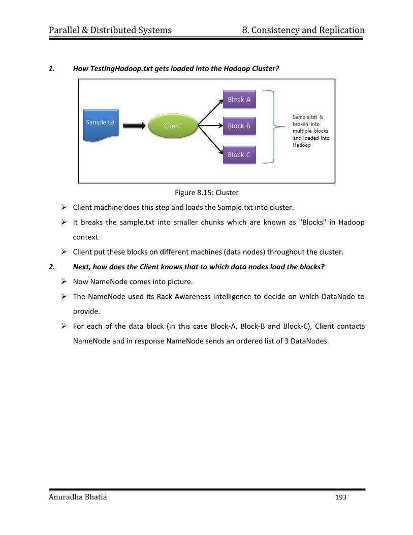
Parallel & Distributed Systems 8. Consistency and Replication
Anuradha Bhatia 193
1. How TestingHadoop.txt gets loaded into the Hadoop Cluster?
Figure 8.15: Cluster
Client machine does this step and loads the Sample.txt into cluster.
It breaks the sample.txt into smaller chunks which are known as "Blocks" in Hadoop
context.
Client put these blocks on different machines (data nodes) throughout the cluster.
2. Next, how does the Client knows that to which data nodes load the blocks?
Now NameNode comes into picture.
The NameNode used its Rack Awareness intelligence to decide on which DataNode to
provide.
For each of the data block (in this case Block-A, Block-B and Block-C), Client contacts
NameNode and in response NameNode sends an ordered list of 3 DataNodes.
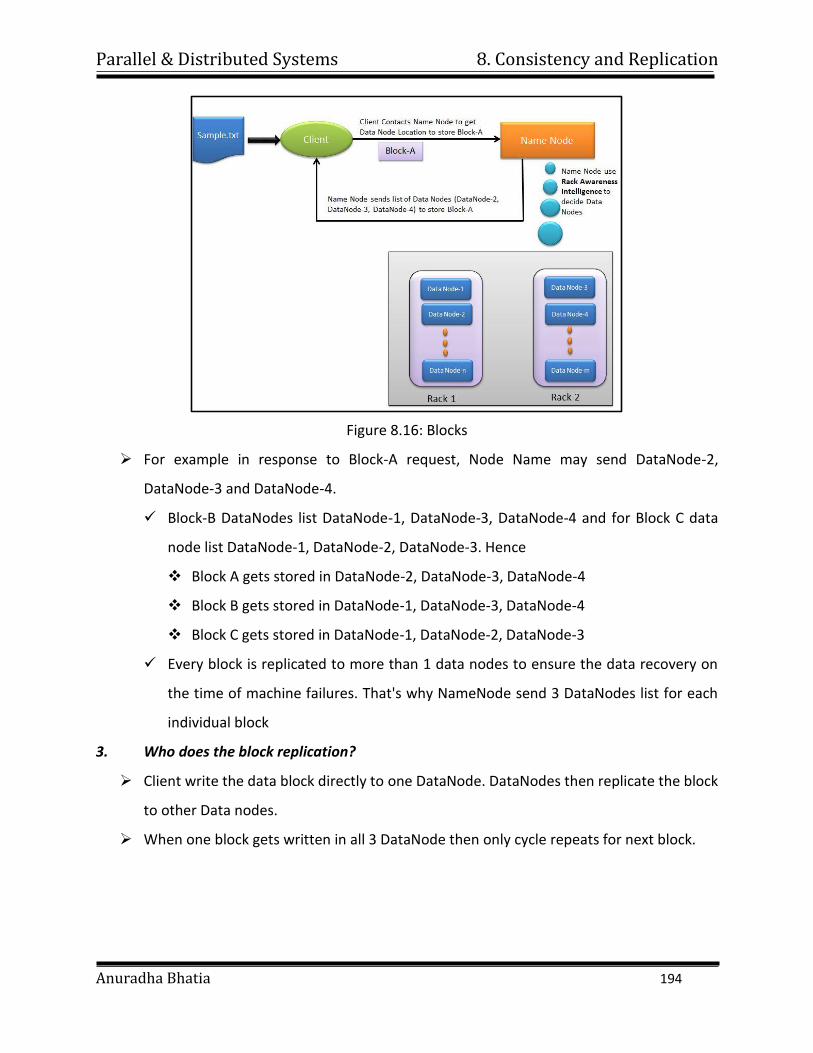
Parallel & Distributed Systems 8. Consistency and Replication
Anuradha Bhatia 194
Figure 8.16: Blocks
For example in response to Block-A request, Node Name may send DataNode-2,
DataNode-3 and DataNode-4.
Block-B DataNodes list DataNode-1, DataNode-3, DataNode-4 and for Block C data
node list DataNode-1, DataNode-2, DataNode-3. Hence
Block A gets stored in DataNode-2, DataNode-3, DataNode-4
Block B gets stored in DataNode-1, DataNode-3, DataNode-4
Block C gets stored in DataNode-1, DataNode-2, DataNode-3
Every block is replicated to more than 1 data nodes to ensure the data recovery on
the time of machine failures. That's why NameNode send 3 DataNodes list for each
individual block
3. Who does the block replication?
Client write the data block directly to one DataNode. DataNodes then replicate the block
to other Data nodes.
When one block gets written in all 3 DataNode then only cycle repeats for next block.
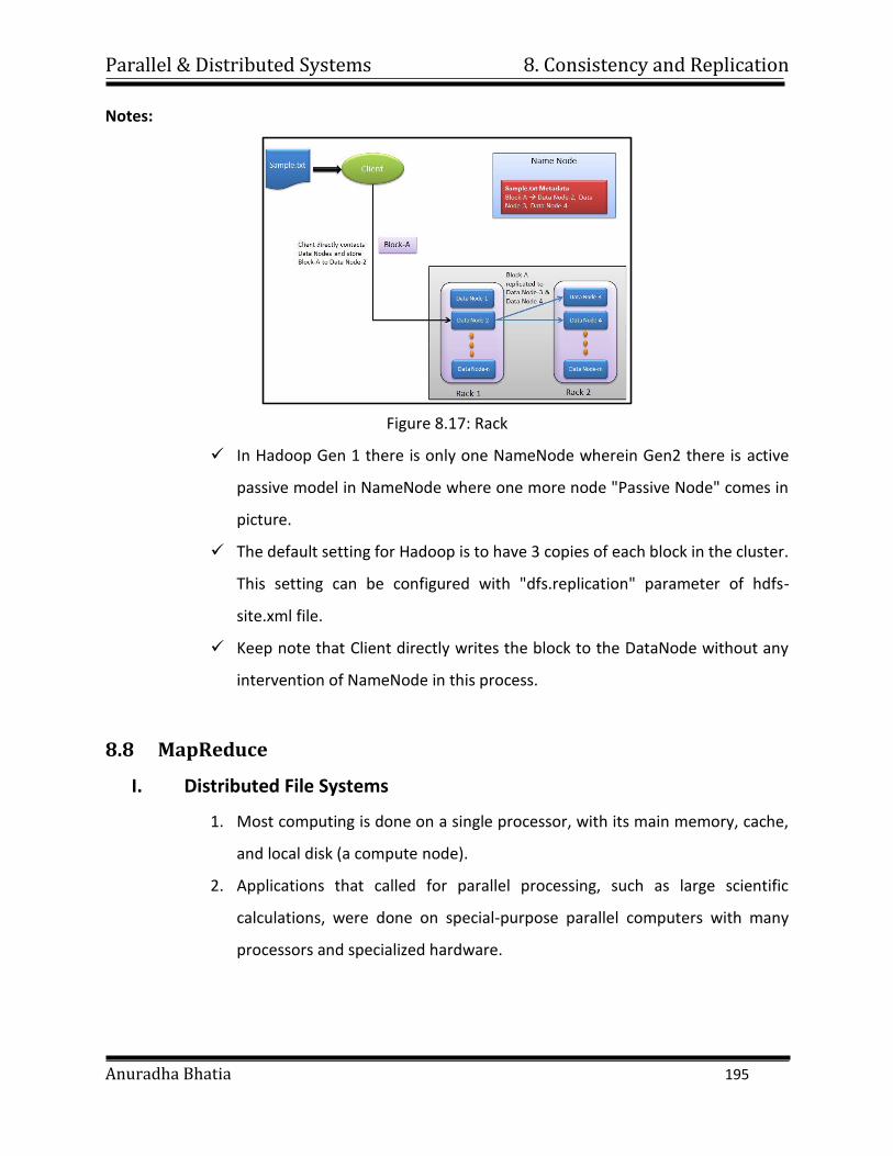
Parallel & Distributed Systems 8. Consistency and Replication
Anuradha Bhatia 195
Notes:
Figure 8.17: Rack
In Hadoop Gen 1 there is only one NameNode wherein Gen2 there is active
passive model in NameNode where one more node "Passive Node" comes in
picture.
The default setting for Hadoop is to have 3 copies of each block in the cluster.
This setting can be configured with "dfs.replication" parameter of hdfs-
site.xml file.
Keep note that Client directly writes the block to the DataNode without any
intervention of NameNode in this process.
8.8 MapReduce
I. Distributed File Systems
1. Most computing is done on a single processor, with its main memory, cache,
and local disk (a compute node).
2. Applications that called for parallel processing, such as large scientific
calculations, were done on special-purpose parallel computers with many
processors and specialized hardware.
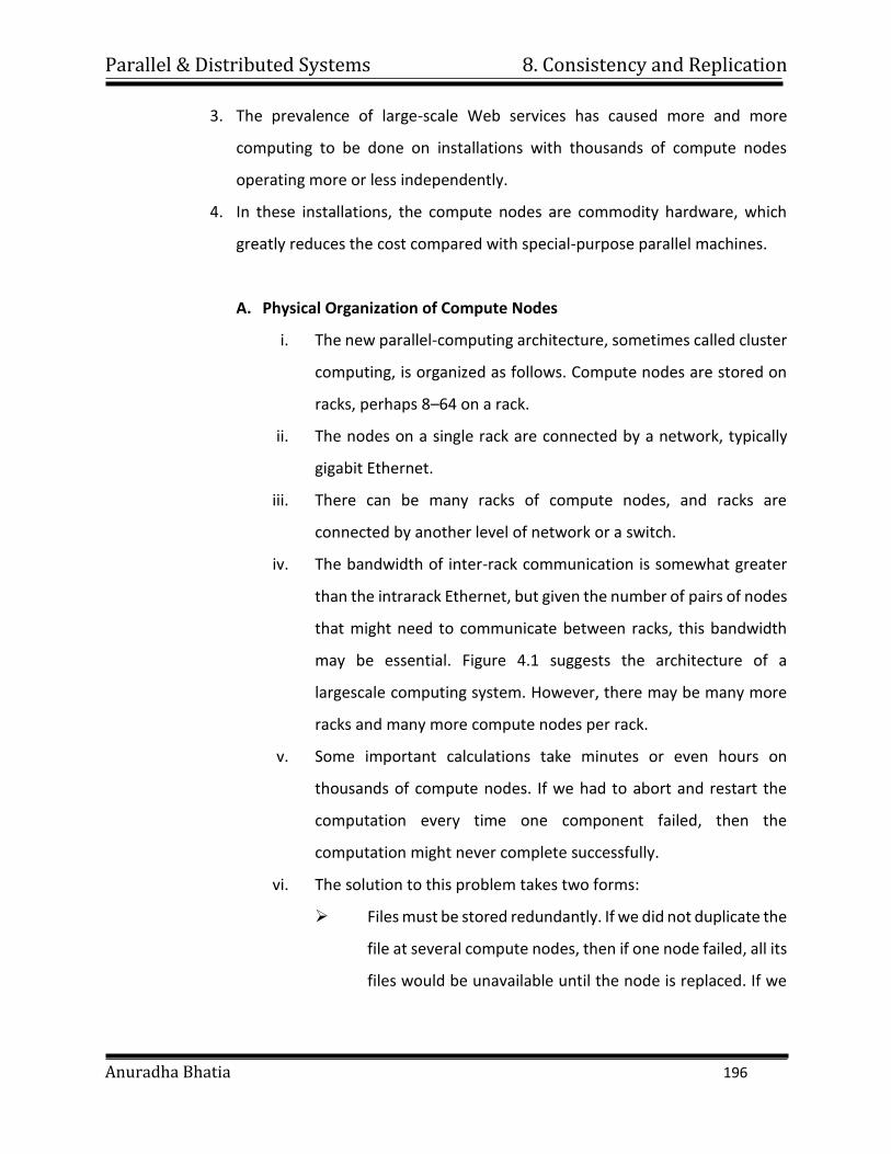
Parallel & Distributed Systems 8. Consistency and Replication
Anuradha Bhatia 196
3. The prevalence of large-scale Web services has caused more and more
computing to be done on installations with thousands of compute nodes
operating more or less independently.
4. In these installations, the compute nodes are commodity hardware, which
greatly reduces the cost compared with special-purpose parallel machines.
A. Physical Organization of Compute Nodes
i. The new parallel-computing architecture, sometimes called cluster
computing, is organized as follows. Compute nodes are stored on
racks, perhaps 8–64 on a rack.
ii. The nodes on a single rack are connected by a network, typically
gigabit Ethernet.
iii. There can be many racks of compute nodes, and racks are
connected by another level of network or a switch.
iv. The bandwidth of inter-rack communication is somewhat greater
than the intrarack Ethernet, but given the number of pairs of nodes
that might need to communicate between racks, this bandwidth
may be essential. Figure 4.1 suggests the architecture of a
largescale computing system. However, there may be many more
racks and many more compute nodes per rack.
v. Some important calculations take minutes or even hours on
thousands of compute nodes. If we had to abort and restart the
computation every time one component failed, then the
computation might never complete successfully.
vi. The solution to this problem takes two forms:
Files must be stored redundantly. If we did not duplicate the
file at several compute nodes, then if one node failed, all its
files would be unavailable until the node is replaced. If we
Parallel & Distributed Systems 8. Consistency and Replication
Anuradha Bhatia 197
did not back up the files at all, and the disk crashes, the files
would be lost forever.
Computations must be divided into tasks, such that if any
one task fails to execute to completion, it can be restarted
without affecting other tasks.
Figure 8.18: Racks of compute nodes
B. Large-Scale File-System Organization
i. To exploit cluster computing, files must look and behave somewhat
differently from the conventional file systems found on single
computers.
ii. This new file system, often called a distributed file system or DFS
(although this term has had other meanings in the past), is typically
used as follows.
iii. There are several distributed file systems of the type we have
described that are used in practice. Among these:
The Google File System (GFS), the original of the class.
Hadoop Distributed File System (HDFS), an open-source DFS
used with Hadoop, an implementation of map-reduce and
distributed by the Apache Software Foundation.
CloudStore, an open-source DFS originally developed by
Kosmix.
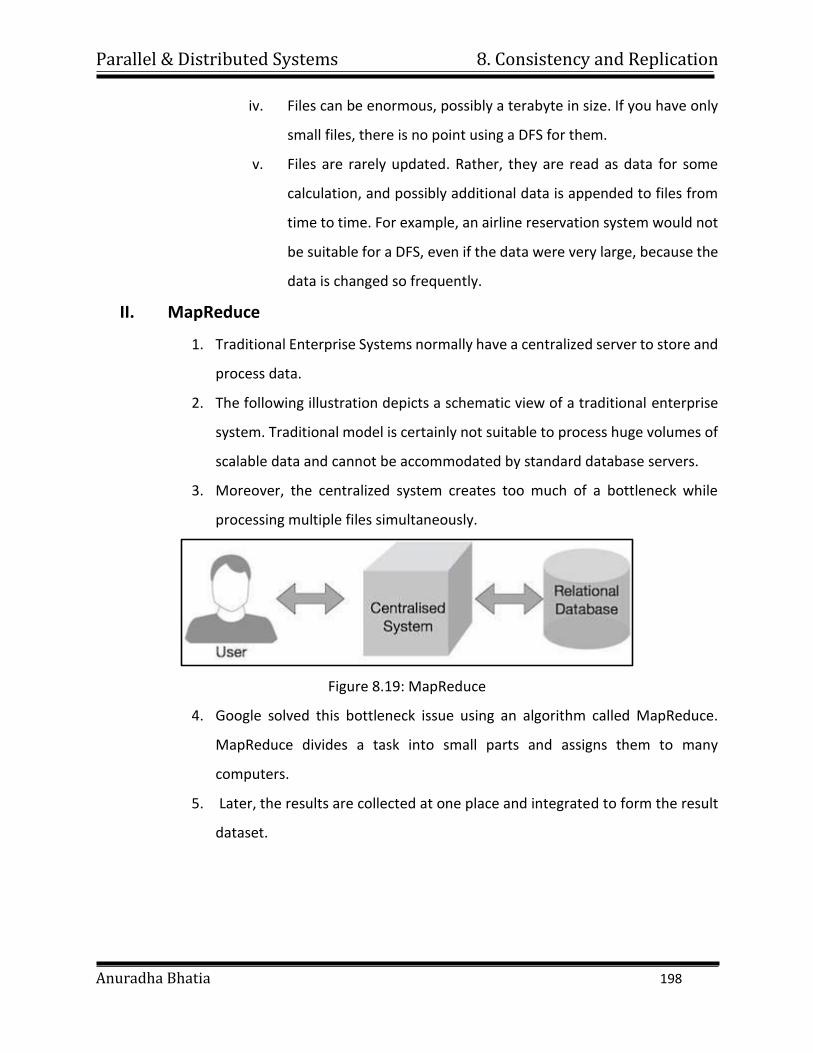
Parallel & Distributed Systems 8. Consistency and Replication
Anuradha Bhatia 198
iv. Files can be enormous, possibly a terabyte in size. If you have only
small files, there is no point using a DFS for them.
v. Files are rarely updated. Rather, they are read as data for some
calculation, and possibly additional data is appended to files from
time to time. For example, an airline reservation system would not
be suitable for a DFS, even if the data were very large, because the
data is changed so frequently.
II. MapReduce
1. Traditional Enterprise Systems normally have a centralized server to store and
process data.
2. The following illustration depicts a schematic view of a traditional enterprise
system. Traditional model is certainly not suitable to process huge volumes of
scalable data and cannot be accommodated by standard database servers.
3. Moreover, the centralized system creates too much of a bottleneck while
processing multiple files simultaneously.
Figure 8.19: MapReduce
4. Google solved this bottleneck issue using an algorithm called MapReduce.
MapReduce divides a task into small parts and assigns them to many
computers.
5. Later, the results are collected at one place and integrated to form the result
dataset.
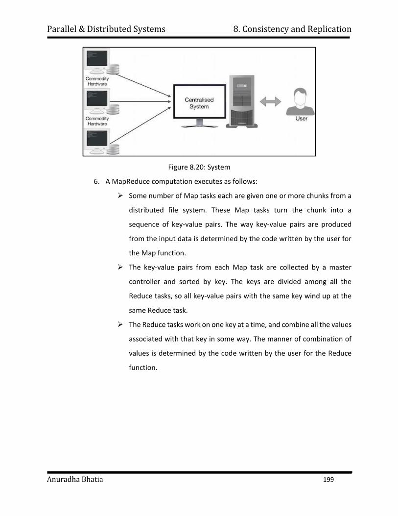
Parallel & Distributed Systems 8. Consistency and Replication
Anuradha Bhatia 199
Figure 8.20: System
6. A MapReduce computation executes as follows:
Some number of Map tasks each are given one or more chunks from a
distributed file system. These Map tasks turn the chunk into a
sequence of key-value pairs. The way key-value pairs are produced
from the input data is determined by the code written by the user for
the Map function.
The key-value pairs from each Map task are collected by a master
controller and sorted by key. The keys are divided among all the
Reduce tasks, so all key-value pairs with the same key wind up at the
same Reduce task.
The Reduce tasks work on one key at a time, and combine all the values
associated with that key in some way. The manner of combination of
values is determined by the code written by the user for the Reduce
function.
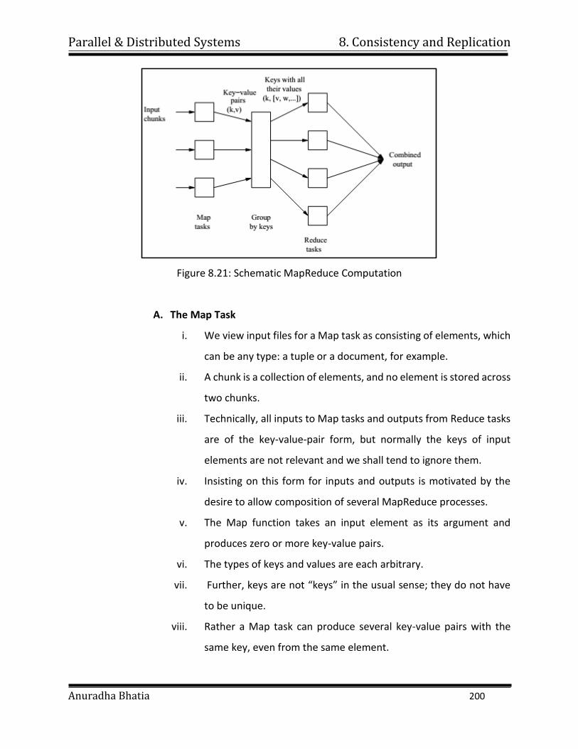
Parallel & Distributed Systems 8. Consistency and Replication
Anuradha Bhatia 200
Figure 8.21: Schematic MapReduce Computation
A. The Map Task
i. We view input files for a Map task as consisting of elements, which
can be any type: a tuple or a document, for example.
ii. A chunk is a collection of elements, and no element is stored across
two chunks.
iii. Technically, all inputs to Map tasks and outputs from Reduce tasks
are of the key-value-pair form, but normally the keys of input
elements are not relevant and we shall tend to ignore them.
iv. Insisting on this form for inputs and outputs is motivated by the
desire to allow composition of several MapReduce processes.
v. The Map function takes an input element as its argument and
produces zero or more key-value pairs.
vi. The types of keys and values are each arbitrary.
vii. Further, keys are not “keys” in the usual sense; they do not have
to be unique.
viii. Rather a Map task can produce several key-value pairs with the
same key, even from the same element.
Parallel & Distributed Systems 8. Consistency and Replication
Anuradha Bhatia 201
B. Grouping by Key
i. As soon as the Map tasks have all completed successfully, the key-
value pairs are grouped by key, and the values associated with each
key are formed into a list of values.
ii. The grouping is performed by the system, regardless of what the
Map and Reduce tasks do.
iii. The master controller process knows how many Reduce tasks there
will be, say r such tasks.
iv. The user typically tells the MapReduce system what r should be.
v. Then the master controller picks a hash function that applies to
keys and produces a bucket number from 0 to r − 1.
vi. Each key that is output by a Map task is hashed and its key-value
pair is put in one of r local files. Each file is destined for one of the
Reduce tasks.1.
vii. To perform the grouping by key and distribution to the Reduce
tasks, the master controller merges the files from each Map task
that are destined for a particular Reduce task and feeds the merged
file to that process as a sequence of key-list-of-value pairs.
viii. That is, for each key k, the input to the Reduce task that handles
key k is a pair of the form (k, [v1, v2, . . . , vn]), where (k, v1), (k, v2),
. . . , (k, vn) are all the key-value pairs with key k coming from all the
Map tasks.
C. The Reduce Task
i. The Reduce function’s argument is a pair consisting of a key and its
list of associated values.
ii. The output of the Reduce function is a sequence of zero or more
key-value pairs.
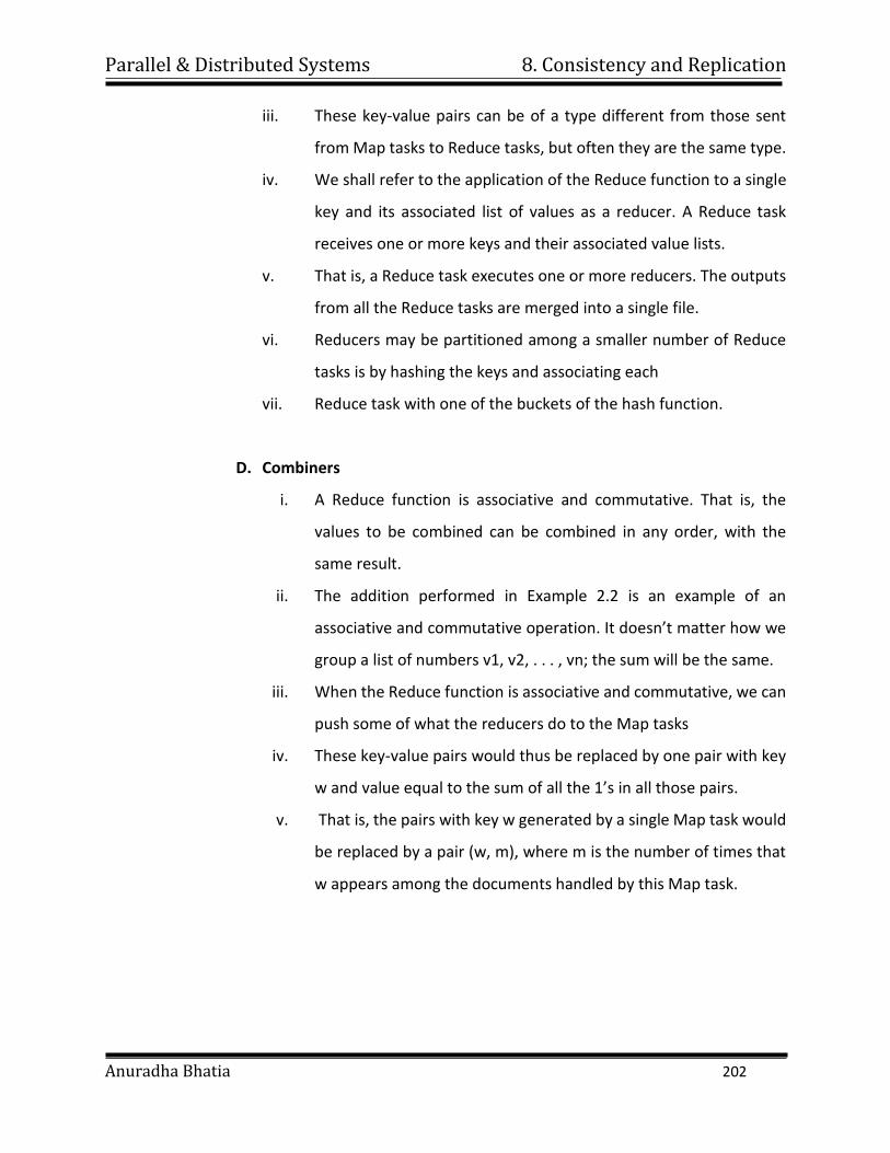
Parallel & Distributed Systems 8. Consistency and Replication
Anuradha Bhatia 202
iii. These key-value pairs can be of a type different from those sent
from Map tasks to Reduce tasks, but often they are the same type.
iv. We shall refer to the application of the Reduce function to a single
key and its associated list of values as a reducer. A Reduce task
receives one or more keys and their associated value lists.
v. That is, a Reduce task executes one or more reducers. The outputs
from all the Reduce tasks are merged into a single file.
vi. Reducers may be partitioned among a smaller number of Reduce
tasks is by hashing the keys and associating each
vii. Reduce task with one of the buckets of the hash function.
D. Combiners
i. A Reduce function is associative and commutative. That is, the
values to be combined can be combined in any order, with the
same result.
ii. The addition performed in Example 2.2 is an example of an
associative and commutative operation. It doesn’t matter how we
group a list of numbers v1, v2, . . . , vn; the sum will be the same.
iii. When the Reduce function is associative and commutative, we can
push some of what the reducers do to the Map tasks
iv. These key-value pairs would thus be replaced by one pair with key
w and value equal to the sum of all the 1’s in all those pairs.
v. That is, the pairs with key w generated by a single Map task would
be replaced by a pair (w, m), where m is the number of times that
w appears among the documents handled by this Map task.
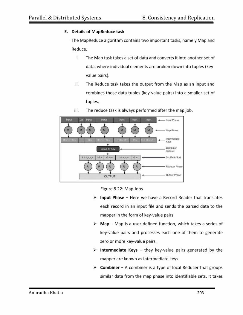
Parallel & Distributed Systems 8. Consistency and Replication
Anuradha Bhatia 203
E. Details of MapReduce task
The MapReduce algorithm contains two important tasks, namely Map and
Reduce.
i. The Map task takes a set of data and converts it into another set of
data, where individual elements are broken down into tuples (key-
value pairs).
ii. The Reduce task takes the output from the Map as an input and
combines those data tuples (key-value pairs) into a smaller set of
tuples.
iii. The reduce task is always performed after the map job.
Figure 8.22: Map Jobs
Input Phase − Here we have a Record Reader that translates
each record in an input file and sends the parsed data to the
mapper in the form of key-value pairs.
Map − Map is a user-defined function, which takes a series of
key-value pairs and processes each one of them to generate
zero or more key-value pairs.
Intermediate Keys − they key-value pairs generated by the
mapper are known as intermediate keys.
Combiner − A combiner is a type of local Reducer that groups
similar data from the map phase into identifiable sets. It takes
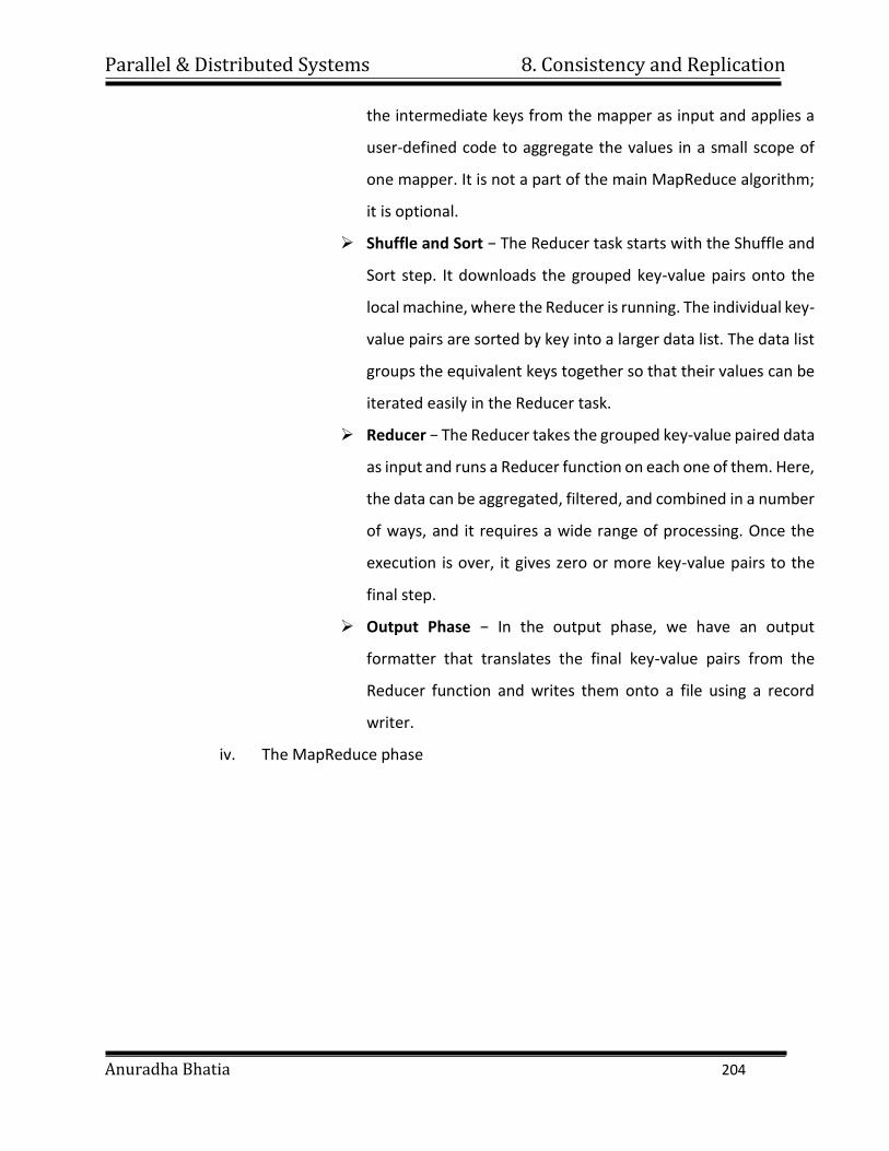
Parallel & Distributed Systems 8. Consistency and Replication
Anuradha Bhatia 204
the intermediate keys from the mapper as input and applies a
user-defined code to aggregate the values in a small scope of
one mapper. It is not a part of the main MapReduce algorithm;
it is optional.
Shuffle and Sort − The Reducer task starts with the Shuffle and
Sort step. It downloads the grouped key-value pairs onto the
local machine, where the Reducer is running. The individual key-
value pairs are sorted by key into a larger data list. The data list
groups the equivalent keys together so that their values can be
iterated easily in the Reducer task.
Reducer − The Reducer takes the grouped key-value paired data
as input and runs a Reducer function on each one of them. Here,
the data can be aggregated, filtered, and combined in a number
of ways, and it requires a wide range of processing. Once the
execution is over, it gives zero or more key-value pairs to the
final step.
Output Phase − In the output phase, we have an output
formatter that translates the final key-value pairs from the
Reducer function and writes them onto a file using a record
writer.
iv. The MapReduce phase
Parallel & Distributed Systems 8. Consistency and Replication
Anuradha Bhatia 205
Figure 8.23: MapReduce Phase
F. MapReduce-Example
Twitter receives around 500 million tweets per day, which is nearly 3000
tweets per second. The following illustration shows how Tweeter manages
its tweets with the help of MapReduce.
Figure 8.25: Twitter Example
i. Tokenize − Tokenizes the tweets into maps of tokens and writes them
as key-value pairs.
ii. Filter − Filters unwanted words from the maps of tokens and writes the
filtered maps as key-value pairs.
iii. Count − Generates a token counter per word.
iv. Aggregate Counters − Prepares an aggregate of similar counter values
into small manageable units.
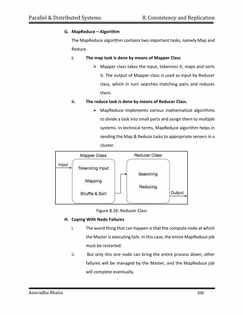
Parallel & Distributed Systems 8. Consistency and Replication
Anuradha Bhatia 206
G. MapReduce – Algorithm
The MapReduce algorithm contains two important tasks, namely Map and
Reduce.
i. The map task is done by means of Mapper Class
Mapper class takes the input, tokenizes it, maps and sorts
it. The output of Mapper class is used as input by Reducer
class, which in turn searches matching pairs and reduces
them.
ii. The reduce task is done by means of Reducer Class.
MapReduce implements various mathematical algorithms
to divide a task into small parts and assign them to multiple
systems. In technical terms, MapReduce algorithm helps in
sending the Map & Reduce tasks to appropriate servers in a
cluster.
Figure 8.26: Reducer Class
H. Coping With Node Failures
i. The worst thing that can happen is that the compute node at which
the Master is executing fails. In this case, the entire MapReduce job
must be restarted.
ii. But only this one node can bring the entire process down; other
failures will be managed by the Master, and the MapReduce job
will complete eventually.
Parallel & Distributed Systems 8. Consistency and Replication
Anuradha Bhatia 207
iii. Suppose the compute node at which a Map worker resides fails.
This failure will be detected by the Master, because it periodically
pings the Worker processes.
iv. All the Map tasks that were assigned to this Worker will have to be
redone, even if they had completed. The reason for redoing
completed Map asks is that their output destined for the Reduce
tasks resides at that compute node, and is now unavailable to the
Reduce tasks.
v. The Master sets the status of each of these Map tasks to idle and
will schedule them on a Worker when one becomes available. The
vi. Master must also inform each Reduce task that the location of its
input from that Map task has changed. Dealing with a failure at the
node of a Reduce worker is simpler.
vii. The Master simply sets the status of its currently executing Reduce
tasks to idle. These will be rescheduled on another reduce worker
later.