Parallel Direction Method of Multipliersbaner029/papers/14/pdmm.pdf · Parallel Direction Method of Multipliers ... behaving like parallel randomized block coordinate descent

Parallel Direction Method of Multipliers

Huahua WangDept of Computer Science and Engineering

University of Minnesota, Twin [email protected]

Arindam BanerjeeDept of Computer Science and Engineering


Zhi-Quan LuoDepartment of Electrical and Computer Engineering


Abstract

We consider the problem of minimizing block-separable convex functions subject to linear con-straints. While the Alternating Direction Method of Multipliers (ADMM) for two-block linear con-straints has been intensively studied both theoretically and empirically, in spite of some preliminarywork, effective generalizations of ADMM to multiple blocks is still unclear. In this paper, we propose arandomized block coordinate method named Parallel Direction Method of Multipliers (PDMM) to solvethe optimization problems with multi-block linear constraints. PDMM randomly updates some primalblocks in parallel, behaving like parallel randomized block coordinate descent. We establish the globalconvergence and the iteration complexity for PDMM with constant step size. We also show that PDMMcan do randomized block coordinate descent on overlapping blocks. Experimental results show thatPDMM performs better than state-of-the-arts methods in two applications, robust principal componentanalysis and overlapping group lasso.

1 Introduction

In this paper, we consider the minimization of block-seperable convex functions subject to linear constraints,with a canonical form:

min{xj∈Xj}

f(x) =J∑j=1

fj(xj) , s.t. Ax =J∑j=1

Acjxj = a , (1)

where the objective function f(x) is a sum of J block separable (nonsmooth) convex functions, Acj ∈

Rm×nj is the j-th column block of A ∈ Rm×n where n =∑

j nj , xj ∈ Rnj×1 is the j-th block coordinateof x, Xj is a local convex constraint of xj and a ∈ Rm×1. The canonical form can be extended to handlelinear inequalities by introducing slack variables, i.e., writing Ax ≤ a as Ax + z = a, z ≥ 0.

A variety of machine learning problems can be cast into the linearly-constrained optimization prob-lem (1). For example, in robust Principal Component Analysis (RPCA) [5], one attempts to recover a lowrank matrix L and a sparse matrix S from an observation matrix M, i.e., the linear constraint is M = L+S.Further, in the stable version of RPCA [43], an noisy matrix Z is taken into consideration, and the linearconstraint has three blocks, i.e., M = L+S+Z. The linear constraint with three blocks also appears in the

1

latent variable Gaussian graphical model selection problem [6, 23]. Problem (1) can also include compositeminimization problems which solve a sum of a loss function and a set of nonsmooth regularization functions.Due to the increasing interest in structural sparsity [2], composite regularizers have become widely used,e.g., overlapping group lasso [42]. As the blocks are overlapping in this class of problems, it is difficult toapply block coordinate descent methods for large scale problem [24, 27] which assume block-separable. Bysimply splitting blocks through introducing equality constraints, the composite minimization problem canalso formulated as (1) [3].

A classical approach to solving (1) is to relax the linear constraints using the (augmented) Lagrangian [28,29], i.e.,

Lρ(x,y) = f(x) + 〈y,Ax− a〉+ρ

2‖Ax− a‖22 . (2)

where ρ ≥ 0 is called the penalty parameter. We call x the primal variable and y the dual variable. (2) usuallyleads to primal-dual algorithms which update the primal and dual variables alternatively. The dual updateis simply dual gradient ascent where the dual gradient is the resiudal of equality constraint, i.e., Ax − a.The primal update is to solve a minimization problem of (2) given y. The primal update determines theefficiency of this class of primal-dual algorithms and will be the focus of this paper.

If ρ = 0, (2) decomposes into J independent subproblems provided f is separable. In this scenario, theprimal-dual algorithm is called the dual ascent method [4, 31], where the primal update is solved in a parallelblock coordinate fashion. While the dual ascent method can achieve massive parallelism, a careful choiceof stepsize and some strict conditions are required for convergence, particularly when f is nonsmooth. Toachieve better numerical efficiency and convergence behavior compared to the dual ascent method, it isfavorable to set ρ > 0 in the augmented Lagrangian (2). However, (2) is no longer separable since theaugmentation term makes x coupled. A well-known primal-dual algorithm to solve (2) is the method ofmultipliers, which solves the primal update in one block. For large scale optimization problems, it is oftendifficult to solve the entire augmented Lagrangian efficiently. Considerable efforts have thus been devotedto solving the primal update of the method of multipliers efficiently. In [34], randomized block coordinatedescent (RBCD) [24, 27] is used to solve (2) exactly, but leading to a double-loop algorithm along with thedual step. More recent results show (2) can be solved inexactly by just sweeping the coordinates once usingthe alternating direction method of multipliers (ADMM) [14, 3].

When J = 2, the constraint is of the form Ac1x1 + Ac

2x2 = a. In this case, a well-known variant ofthe method of multipliers is the Alternating Direction Method of Multipliers (ADMM) [3], which solvesthe augmented Lagrangian seperately and alternatively. ADMM was first introduced in [14] and becomepopular in recent years due to its ease of applicability and superior empirical performance in a wide varietyof applications, ranging from image processing [11, 1, 15] to applied statistics and machine learning [30,40, 39, 22, 35, 12, 21, 37]. For further understanding of ADMM with two blocks, we refer the readersto the comprehensive review by [3]. The proof of global convergence of ADMM with two blocks can befound in [13, 3]. Recently, it has been shown that ADMM converges at a rate of O(1/T ) [35, 18], whereT is the number of iterations. For strongly convex functions, the dual objective of an accelerated versionof ADMM can converge at a rate of O(1/T 2) [16]. For strongly convex functions, ADMM can achieve alinear convergence rate [10].

Encouraged by the success of ADMM with two blocks, ADMM has also been extended to solve theproblem with multiple blocks [20, 19, 9, 26, 17, 7]. The variants of ADMM can be mainly divided into twocategories. One is Gauss-Seidel ADMM (GSADMM) [20, 19], which solves (2) in a cyclic block coordinatemanner. [20] established a linear convergence rate for MADMM under some fairly strict conditions: (1) Aj

has full column rank; (2) fj has Lipschitz-continuous gradients; (3) certain local error bounds hold; (4) the

2

step size needs to be sufficiently small. In [17], a back substitution step was added so that the convergenceof ADMM for multiple blocks can be proved. In some cases, it has been shown that ADMM might not con-verge for multiple blocks [7]. In [19], a block successive upper bound minimization method of multipliers(BSUMM) is proposed to solve the problem (1). The convergence of BSUMM is established under condi-tions: (i) certain local error bounds hold; (ii) the step size is either sufficiently small or decreasing. However,in general, Gauss-Seidel ADMM with multiple blocks is not well understood and its iteration complexityis largely open. The other is Jacobi ADMM [38, 9, 26], which solves (2) in a parallel block coordinatefashion. In [38, 26], (1) is solved by using two-block ADMM with splitting variables (sADMM). [9] con-siders a proximal Jacobian ADMM (PJADMM) by adding proximal terms. In addition to the two typesof extensions, a randomized block coordinate variant of ADMM named RBSUMM was proposed in [19].However, RBSUMM can only randomly update one block. Moreover, the convergence of RBSUMM isestablished under the same conditions as BSUMM and its iteration complexity is unknown. In [32], ADMMwith stochastic dual coordinate ascent is proposed to solve online or stochastic ADMM [35, 25, 33] problemin the dual, which is not the focus of this paper.

In this paper, we propose a randomized block coordinate method named parallel direction method ofmultipliers (PDMM) which randomly picks up any number of blocks to update in parallel, behaving likerandomized block coordinate descent [24, 27]. Like the dual ascent method, PDMM solves the primalupdate in a parallel block coordinate fashion even with the augmentation term. Moreover, PDMM inheritsthe merits of the method of multipliers and can solve a fairly large class of problems, including nonsmoothfunctions. Technically, PDMM has three aspects which make it distinct from such state-of-the-art methods.First, if block coordinates of the primal x is solved exactly, PDMM uses a backward step on the dual updateso that the dual variable makes conservative progress. Second, the sparsity of A and the number of blocksKto be updated are taken into consideration to determine the step size of the dual update. Third, PDMM canrandomly choose arbitrary number of primal blocks for update in parallel. Moreover, we show that sADMMand PJADMM are the two extreme cases of PDMM. The connection between sADMM and PJADMMthrough PDMM provides better understanding of dual backward step. PDMM can also be used to solveoverlapping groups in a randomized block coordinate fashion. Interestingly, the corresponding problem forRBCD [24, 27] with overlapping blocks is still an open problem. We establish the global convergence andO(1/T ) iteration complexity of PDMM with constant step size. We evaluate the performance of PDMM intwo applications: robust principal component analysis and overlapping group lasso.

The rest of the paper is organized as follows. PDMM is proposed in Section 2. The convergence resultsare established in Section 3. We evaluate the performance of PDMM in Section 5 and conclude the paper inSection 6. The proof of the convergence of PDMM is given in the Appendix.

Notations: Assume that A ∈ Rm×n is divided into I × J blocks. Let Ari ∈ Rmi×n be the i-th row

block of A, Acj ∈ Rm×nj be the j-th column block of A, and Aij ∈ Rmi×nj be the ij-th block of A. Let

yi ∈ Rmi×1 be the i-th block coordinate of y ∈ Rm×1. N (i) is a set of nonzero blocks Aij in the i-throw block Ar

i and di = |N (i)| is the number of nonzero blocks. λijmax is the largest eigenvalue of ATijAij .

diag(x) denotes a diagonal matrix of vector x. In is an identity matrix of size n×n. Let Ki = min{di,K}where K is the number of blocks randomly chosen by PDMM and T be the number of iterations.

3

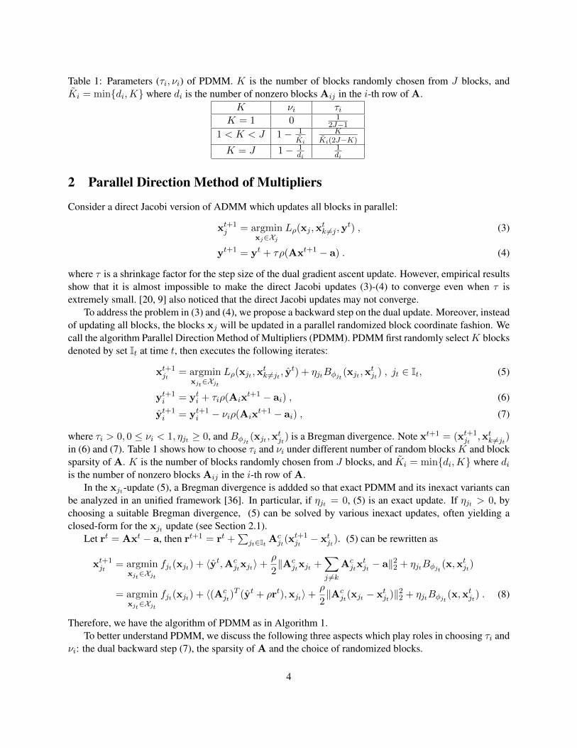
Table 1: Parameters (τi, νi) of PDMM. K is the number of blocks randomly chosen from J blocks, andKi = min{di,K} where di is the number of nonzero blocks Aij in the i-th row of A.

K νi τiK = 1 0 1

2J−11 < K < J 1− 1

Ki

KKi(2J−K)

K = J 1− 1di

1di

2 Parallel Direction Method of Multipliers

Consider a direct Jacobi version of ADMM which updates all blocks in parallel:

xt+1j = argmin

xj∈Xj

Lρ(xj ,xtk 6=j ,y

t) , (3)

yt+1 = yt + τρ(Axt+1 − a) . (4)

where τ is a shrinkage factor for the step size of the dual gradient ascent update. However, empirical resultsshow that it is almost impossible to make the direct Jacobi updates (3)-(4) to converge even when τ isextremely small. [20, 9] also noticed that the direct Jacobi updates may not converge.

To address the problem in (3) and (4), we propose a backward step on the dual update. Moreover, insteadof updating all blocks, the blocks xj will be updated in a parallel randomized block coordinate fashion. Wecall the algorithm Parallel Direction Method of Multipliers (PDMM). PDMM first randomly selectK blocksdenoted by set It at time t, then executes the following iterates:

xt+1jt

= argminxjt∈Xjt

Lρ(xjt ,xtk 6=jt , y

t) + ηjtBφjt (xjt ,xtjt) , jt ∈ It, (5)

yt+1i = yti + τiρ(Aix

t+1 − ai) , (6)

yt+1i = yt+1

i − νiρ(Aixt+1 − ai) , (7)

where τi > 0, 0 ≤ νi < 1, ηjt ≥ 0, and Bφjt (xjt ,xtjt

) is a Bregman divergence. Note xt+1 = (xt+1jt

,xtk 6=jt)in (6) and (7). Table 1 shows how to choose τi and νi under different number of random blocks K and blocksparsity of A. K is the number of blocks randomly chosen from J blocks, and Ki = min{di,K} where diis the number of nonzero blocks Aij in the i-th row of A.

In the xjt-update (5), a Bregman divergence is addded so that exact PDMM and its inexact variants canbe analyzed in an unified framework [36]. In particular, if ηjt = 0, (5) is an exact update. If ηjt > 0, bychoosing a suitable Bregman divergence, (5) can be solved by various inexact updates, often yielding aclosed-form for the xjt update (see Section 2.1).

Let rt = Axt − a, then rt+1 = rt +∑

jt∈It Acjt

(xt+1jt− xtjt). (5) can be rewritten as

xt+1jt

= argminxjt∈Xjt

fjt(xjt) + 〈yt,Acjtxjt〉+

ρ

2‖Ac

jtxjt +∑j 6=k

Acjtx

tjt − a‖22 + ηjtBφjt (x,x

tjt)

= argminxjt∈Xjt

fjt(xjt) + 〈(Acjt)

T (yt + ρrt),xjt〉+ρ

2‖Ac

jt(xjt − xtjt)‖22 + ηjtBφjt (x,x

tjt) . (8)

Therefore, we have the algorithm of PDMM as in Algorithm 1.To better understand PDMM, we discuss the following three aspects which play roles in choosing τi and

νi: the dual backward step (7), the sparsity of A and the choice of randomized blocks.

4

Algorithm 1 Parallel Diretion Method of Multipliers1: Input: ρ, ηj , τi, νi2: Initialization: x1, y1 = 03: if τi, νi are not defined, initialize τi, νi as given in Table 14: r1 = Ax1 − a = −a5: for t = 1 to T do6: randomly pick up jt block coordinates7: xt+1

jt= argmin

xjt∈Xjt

fjt(xjt) + 〈(Acjt

)T (yt + ρrt),xjt〉+ ρ2‖A

cjt

(xjt − xtjt)‖22 + ηjtBφjt (x,x

tjt

)

8: rt+1 = rt +∑

jt∈It Acjt

(xt+1jt− xtjt)

9: yt+1i = yti + τiρr

t+1i

10: yt+1i = yt+1

i − νiρrt+1i

11: end for

Dual Backward Step: We attribute the failure of the Jacobi updates (3)-(4) to the following observationin (3), which can be rewritten as:

xt+1j = argmin

xj∈Xj

fj(xj) + 〈yt + ρ(Axt − a),Acjxj〉+

ρ

2‖Ac

j(xj − xtj)‖22 . (9)

In the primal xj update, the quadratic penalty term implicitly adds full gradient ascent step to the dualvariable, i.e., yt + ρ(Axt − a), which we call implicit dual ascent. The implicit dual ascent along withthe explicit dual ascent (4) may lead to too aggressive progress on the dual variable, particularly when thenumber of blocks is large. Based on this observation, we introduce an intermediate variable yt to replaceyt in (9) so that the implicit dual ascent in (9) makes conservative progress, e.g., yt + ρ(Axt − a) =yt + (1− ν)ρ(Axt − a) , where 0 < ν < 1. yt is the result of a ‘backward step’ on the dual variable, i.e.,yt = yt − νρ(Axt − a).

Moreover, one can show that τ and ν have also been implicitly used when using two-block ADMM withsplitting variables (sADMM) to solve (1) [26, 38]. Section 2.2 shows sADMM is a special case of PDMM.The connection helps in understanding the role of the two parameters τi, νi in PDMM. Interestingly, the stepsizes τi and νi can be improved by considering the block sparsity of A and the number of random blocks Kto be updated.

Sparsity of A: Assume A is divided into I × J blocks. While xj can be updated in parallel, thematrix multiplication Ax in the dual update (4) requires synchronization to gather messages from all blockcoordinates jt ∈ It. For updating the i-th block of the dual yi, we need Aix

t+1 =∑

jt∈It Aijtxt+1jt

+∑k/∈It Aikx

tk which aggregates “messages” from all xjt . If Aijt is a block of zeros, there is no “message”

from xjt to yi. More precisely, Aixt+1 =

∑jt∈It∩N (i)Aijtx

t+1jt

+∑

k/∈It Aikxtk whereN (i) denotes a set

of nonzero blocks in the i-th row block Ai. N (i) can be considered as the set of neighbors of the i-th dualblock yi and di = |N (i)| is the degree of the i-th dual block yi. If A is sparse, di could be far smaller thanJ . According to Table 1, a low di will lead to bigger step sizes τi for the dual update and smaller step sizesfor the dual backward step (7). Further, as shown in Section 2.3, when using PDMM with all blocks to solvecomposite minimization with overlapping blocks, PDMM can use τi = 0.5 which is much larger than 1/Jin sADMM.

Randomized Blocks: The number of blocks to be randomly chosen also has the effect on τi, νi. Ifrandomly choosing one block (K = 1), then νi = 0, τi = 1

2J−1 . The dual backward step (7) vanishes. AsK increases, νi increases from 0 to 1− 1

diand τi increases from 1

2J−1 to 1di

. If updating all blocks (K = J),

5

τi = 1di, νi = 1− 1

di.

PDMM does not necessarily choose any K combination of J blocks. The J blocks can be randomlypartitioned into J/K groups where each group has K blocks. Then PDMM randomly picks one group. Asimple way is to permutate the J blocks and choose K blocks cyclically.

2.1 Inexact PDMM

If ηjt > 0, there is an extra Bregman divergence term in (5), which can serve two purposes. First, choosinga suitable Bregman divergence can lead to a closed-form solution for (5). Second, if ηjt is sufficiently large,the dual update can use a large step size (τi = 1) and the backward step (7) can be removed (νi = 0), leadingto the same updates as PJADMM [9] (see Section 2.2).

Given a differentiable function ψjt , its Bregman divergence is defiend as

Bψjt(xjt ,x

tjt)=ψjt(xjt)−ψjt(xtjt)−〈∇ψjt(x

tjt),xjt−x

tjt〉, (10)

where∇ψjt denotes the gradient of ψjt . Rearranging the terms yields

ψjt(xjt)−Bψjt(xjt ,x

tjt)=ψjt(x

tjt)+〈∇ψjt(xtjt),xjt−x

tjt〉, (11)

which is exactly the linearization of ψjt(xjt) at xtjt . Therefore, if solving (5) exactly becomes difficult due tosome problematic terms, we can use the Bregman divergence to linearize these problematic terms so that (5)can be solved efficiently. More specifically, in (5), we can choose φjt = ϕjt − 1

ηjtψjt assuming ψjt is the

problematic term. Using the linearity of Bregman divergence,

Bφjt (xjt ,xtjt) = Bϕjt

(xjt ,xtjt)−

1

ηjtBψjt

(xjt ,xtjt) . (12)

For instance, if fjt is a logistic function, solving (5) exactly requires an iterative algorithm. Settingψjt = fjt ,ϕjt = 1

2‖· ‖22 in (12) and plugging into (5) yield

xt+1jt

= argminxjt∈Xjt

〈∇fjt(xtjt),xjt〉+ 〈yt,Ajtxjt〉

+ρ

2‖Ajtxjt +

∑k 6=j

Akxtk − a‖22 + ηjt‖xjt − xtjt‖

22 , (13)

which has a closed-form solution. Similarly, if the quadratic penalty term ρ2‖A

cjtxjt +

∑k 6=j A

ckxjt − a‖22

is a problematic term, we can set ψjt(xjt) = ρ2‖A

cjtxjt‖22, then Bψjt

(xjt ,xtjt

) = ρ2‖A

cjt

(xjt − xtjt)‖22 can

be used to linearize the quadratic penalty term.In (12), the nonnegativeness of Bφjt implies that Bϕjt

≥ 1ηjtBψjt

. This condition can be satisfiedas long as ϕjt is more convex than ψjt . Technically, we assume that ϕjt is σ/ηjt-strongly convex andψjt has Lipschitz continuous gradient with constant σ, which has been shown in [36]. For instance, ifψjt(xjt) = ρ

2‖Acjtxjt‖22, σ = ρλmax(Ac

jt) where λmax(Ac

jt) denotes the largest eigenvalue of (Ac

jt)TAc

jt.

If choosing ϕjt = 12‖· ‖

22, the condition is satisfied by setting ηjt ≥ ρλmax(Ac

jt).

2.2 Connections to Related Work

All blocks: There are also two other methods which update all blocks in parallel. If solving the primalupdates exactly, two-block ADMM with splitting variables (sADMM) is considered in [26, 38]. We show

6

that sADMM is a special case of PDMM when setting τi = 1J and νi = 1 − 1

J ( See Appendix B). Ifthe primal updates are solved inexactly, [9] considers a proximal Jacobian ADMM (PJADMM) by addingproximal terms where the converge rate is improved to o(1/T ) given the sufficiently large proximal terms.We show that PJADMM [9] is also a special case of PDMM ( See Appendix C). sADMM and PJADMMare two extreme cases of PDMM. The connection between sADMM and PJADMM through PDMM canprovide better understanding of the three methods and the role of dual backward step. If the primal updateis solved exactly which makes sufficient progress, the dual update should take small step, e.g., sADMM. Onthe other hand, if the primal update takes small progress by adding proximal terms, the dual update can takefull gradient step, e.g. PJADMM. While sADMM is a direct derivation of ADMM, PJADMM introducesmore terms and parameters.

Randomized blocks: While PDMM can randomly update any number of blocks, RBUSMM [19] canonly randomly update one block. The convergence of RBSUMM requires certain local error bounds to behold and decreasing step size. Moreover, the iteration complexity of RBSUMM is still unknown. In contast,PDMM converges at a rate of O(1/T ) with the constant step size.

2.3 Randomized Overlapping Block Coordinate

Consider the composite minimization problem of a sum of a loss function `(w) and composite regularizersgj(wj):

minw

`(w) +L∑j=1

gj(wj) , (14)

which considers L overlapping groups wj ∈ Rb×1. Let J = L + 1,xJ = w. For 1 ≤ j ≤ L, denotexj = wj , then xj = UT

j xJ , where Uj ∈ Rb×L is the columns of an identity matrix and extracts thecoordinates of xJ . Denote U = [U1, · · · ,UL] ∈ Rn×(bL) and A = [IbL,−UT ] where bL denotes b × L.By letting fj(xj) = gj(wj) and fJ(xJ) = `(w), (14) can be written as:

minx

J∑j=1

fj(xj) s.t. Ax = 0. (15)

where x = [x1; · · · ;xL;xL+1] ∈ Rb×J . (15) can be solved by PDMM in a randomized block coor-dinate fashion. In A, for b rows block, there are only two nonzero blocks, i.e., di = 2. Therefore,τi = K

2(2J−K) , νi = 0.5. In particular, if K = J , τi = νi = 0.5. In contrast, sADMM uses τi =

1/J � 0.5, νi = 1− 1/J > 0.5 if J is larger.

Remark 1 (a) ADMM [3] can solve (15) where the equality constraint is xj = UTj xJ .

(b) In this setting, Gauss-Seidel ADMM (GSADMM) and BSUMM [19] are the same as ADMM.BSUMM should converge with constant stepsize ρ (not necessarily sufficiently small), although the the-ory of BSUMM does not include this special case.

(c) Consensus optimization [3] has the same formulation as (15). Therefore, PDMM can also be used asa randomized consensus optimization algorithm.

3 Theoretical Results

We establish the convergence results for PDMM under fairly simple assumptions:

7

Assumption 1(1) fj : Rnj → R ∪ {+∞} are closed, proper, and convex.(2) A KKT point of the Lagrangian (ρ = 0 in (2)) of Problem (1) exists.

Assumption 2 is the same as that required by ADMM [3, 35]. Assume that {x∗j ,y∗i } satisfies the KKTconditions of the Lagrangian (ρ = 0 in (2)), i.e.,

−ATj y∗ ∈ ∂fj(x∗j ) , (16)

Ax∗ − a = 0. (17)

During iterations, (82) is satisfied if Axt+1 = a. Let ∂fj be the subdifferential of fj . The optimalityconditions for the xj update (5) is

−Acj [y

t+(1−ν)ρ(Axt − a)+Acj(x

t+1j −x

tj)]−ηj(∇φj(xt+1

j )−∇φj(xtj))∈∂fj(xt+1j ) . (18)

When Axt+1 = a, yt+1 = yt. If Acj(x

t+1j − xtj) = 0, then Axt − a = 0. When ηj ≥ 0, further

assuming Bφj (xt+1j ,xtj) = 0, (81) will be satisfied. Overall, the KKT conditions (81)-(82) are satisfied if

the following optimality conditions are satisfied by the iterates:

Axt+1 = a ,Acj(x

t+1j − xtj) = 0 , (19)

Bφj (xt+1j ,xtj) = 0 . (20)

The above optimality conditions are sufficient for the KKT conditions. (85) are the optimality conditions forthe exact PDMM. (86) is needed only when ηj > 0.

Let zij = Aijxj ∈ Rmi×1, zri = [zTi1, · · · , zTiJ ]T ∈ RmiJ×1 and z = [(zr1)T , · · · , (zrI)T ]T ∈ RJm×1.

Define the residual of optimality conditions (85)-(86) as

R(xt+1) =ρ

2‖zt+1 − zt‖2Pt

+ρ

2

I∑i=1

βi‖Arix

t+1 − ai‖22 +J∑j=1

ηjBφj (xt+1j ,xtj) . (21)

where Pt is some positive semi-definite matrix1 and βi = KJKi

. If R(xt+1) → 0, (85)-(86) will be satis-fied and thus PDMM converges to the KKT point {x∗,y∗}. Define the current iterate vt = (xtj ,y

ti) and

h(v∗,vt) as a distance from vt to a KKT point v∗ = (x∗j ,y∗i ):

h(v∗,vt) =K

J

I∑i=1

1

2τiρ‖y∗i − yt−1i ‖

22 + Lρ(xt,yt) +

ρ

2‖z∗ − zt‖2Q +

J∑j=1

ηjBφj (x∗j ,x

tj) , (22)

where Q is a positive semi-definite matrix1 and Lρ(xt,yt) with γi = 2(J−K)

Ki(2J−K)+ 1

di− K

JKiis

Lρ(xt,yt) = f(xt)− f(x∗) +I∑i=1

{〈yti,Ar

ixt − ai〉+

(γi − τi)ρ2

‖Arix

t − ai‖22}. (23)

The following Lemma shows that h(v∗,vt) ≥ 0.

1See the definition in the Appendix A.

8

Lemma 1 Let vt = (xtj ,yti) be generated by PDMM (5)-(7) and h(v∗,vt) be defined in (89). Setting

νi = 1− 1Ki

and τi = KKi(2J−K)

, we have

h(v∗,vt) ≥ ρ

2

I∑i=1

ζi‖Arix

t − ai‖22 +ρ

2‖z∗ − zt‖2Q + +

J∑j=1

ηjBφj (x∗j ,x

tj) ≥ 0 . (24)

where ζi = J−KKi(2J−K)

+ 1di− K

JKi≥ 0. Moreover, if h(v∗,vt) = 0, then Ar

ixt = ai, z

t = z∗ and

Bφj (x∗j ,x

tj) = 0. Thus, (16)-(17) are satisfied.

In PDMM, yt+1 depends on xt+1, which in turn depends on It. xt and yt are independent of It. xt

depends on the observed realizations of the random variable

ξt−1 = {I1, · · · , It−1} . (25)

The following theorem shows that h(v∗,vt) decreases monotonically and thus establishes the globalconvergence of PDMM.

Theorem 1 (Global Convergence of PDMM) Let vt = (xtj ,yti) be generated by PDMM (5)-(7) and v∗ =

(x∗j ,y∗i ) be a KKT point satisfying (16)-(17). Setting νi = 1− 1

Kiand τi = K

Ki(2J−K), we have

0 ≤ Eξth(v∗,vt+1) ≤ Eξt−1h(v∗,vt) , EξtR(xt+1)→ 0 . (26)

The following theorem establishes the iteration complexity of PDMM in an ergodic sense.

Theorem 2 (The Rate of Convergence) Let (xtj ,yti) be generated by PDMM (5)-(7). Let xT =

∑Tt=1 x

t.Setting νi = 1− 1

Kiand τi = K

Ki(2J−K), we have

Ef(xT )− f(x∗) ≤JK

{∑Ii=1

12βiρ‖y∗i ‖22 + Lρ(x1,y1) + ρ

2‖z∗ − z1‖2Q +

∑Jj=1 ηjBφj (x

∗j ,x

1j )}

T, (27)

EI∑i=1

βi‖Ari x

T − ai‖22 ≤2ρh(v∗,v0)

T. (28)

where βi = KJKi

and Q is a positive semi-definite matrix.

4 Extensions: PDMM with Randomized Dual Block Coordinate Ascent

In this section, we further show that PDMM can update the dual blocks randomly. The randomized dualblock coordinate ascent (RDBCD) can further increase of dual step size τi. More specifically, at time t+ 1,PDMM randomly selectsK primal blocks denoted by Jt andKI dual blocks denoted by set It, then executesthe following iterates:

yt+1i = yt+1

i − νiρ(Aixt+1 − ai) , (29)

xt+1jt

= argminxjt∈Xjt

Lρ(xjt ,xtk 6=jt , y

t) + ηjtBφjt (xjt ,xtjt) , jt ∈ Jt , (30)

yt+1it

= ytit + τitρ(Aitxt+1 − ait) , it ∈ It , (31)

9

where x = (xt+1jt∈Jt ,xk 6∈Jt),y = (yt+1

it∈It ,ytk 6∈∈It), and τi, νi take the following values:

τi =K

Ki[(2J −K)KII +K(1− KI

I )]≥ K

Ki(2J −K), νi = 1− 1

Ki

. (32)

The dual step size τi increases when using RDBCD. If I = J,KI = K = 1, τi = I3J−2 >

13 , which is far

greater than 12J−1 in PDMM without RDBCD.

In this setting, xt+1 depends on Jt, and yt+1 depends on It, Jt. yt+1 depends on xt+1, which in turndepends on the observed realizations of the random variable

ξt = {(I1, J1), · · · , (It, Jt)} . (33)

Define the current iterate vt = (xtj ,yti) and h(v∗,vt) as a distance from vt to a KKT point v∗ =

(x∗j ,y∗i ):

h(v∗,vt) =K

J

I∑i=1

I

2KIτiρ‖y∗i − yt−1i ‖

22 + Lρ(xt,yt) +

ρ

2‖z∗ − zt‖2Q + ηTBφ(x∗,xt) . (34)


Lemma 2 Let h(v∗,vt) be defined in (34). Setting νi = 1− 1Ki

and τi = K

Ki[(2J−K)KII

+K(1−KII

)], we have

h(v∗,vt) ≥ ρ

2

I∑i=1

ζi‖Arix

t − ai‖22 +ρ

2‖z∗ − zt‖2Q + +

J∑j=1

ηjBφj (x∗j ,x

tj) ≥ 0 . (35)

where ζi =(J−K)

KII

+K(1−KII

)

Ki[(2J−K)KII

+K(1−KII

)]+ 1

di− K


ixt = ai, z

t = z∗

and Bφj (x∗j ,x



Theorem 3 (Global Convergence) Let vt = (xtjt ,ytit

) be generated by PDMM (29)-(31) and v∗ = (x∗j ,y∗i )

be a KKT point satisfying (16)-(17). Setting νi = 1− 1Ki

and τi = K

Ki[(2J−K)KII

+K(1−KII

)], we have


Theorem 4 (The Rate of Convergence) Let (xtjt ,ytit

) be generated by PDMM (29)-(31). Let xT =∑Tt=1 x

t. Setting νi = 1− 1Ki

and τi = K

Ki[(2J−K)KII

+K(1−KII

)], we have

Ef(xT )− f(x∗) ≤IKI

∑Ii=1

12τiρ‖y0

i ‖22 + JK

{1

2βiρ‖y∗i ‖22 + Lρ(x1,y1) + ρ

2‖z∗ − z1‖2Q + ηTBφ(x∗,x1)

}T

,

(37)

EI∑i=1

βi‖Ari x

T − ai‖22 ≤2ρh(v∗,v0)

T. (38)

where βi = KJKi

.

10

0 100 200 300 400 500 600 700 800−5

−4

−3

−2

−1

0

1

2

3

4

time (s)

re

sid

ua

l (l

og

)

PDMM1

PDMM2

PDMM3

GSADMM

RBSUMM

sADMM

0 50 100 150 200 250−5

−4

−3

−2

−1

0

1

2

3

4

iterations

re

sid

ua

l (l

og

)

PDMM1

PDMM2

PDMM3

GSADMM

RBSUMM

sADMM

50 100 150 200 250 3007.8

7.85

7.9

7.95

8

8.05

8.1

8.15

time (s)

ob

jec

tiv

e (

log

)

PDMM1

PDMM2

PDMM3

GSADMM

RBSUMM

sADMM

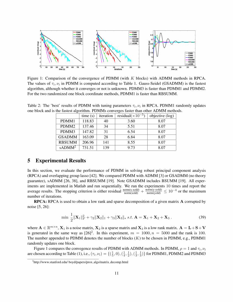
Figure 1: Comparison of the convergence of PDMM (with K blocks) with ADMM methods in RPCA.The values of τi, νi in PDMM is computed according to Table 1. Gauss-Seidel (GSADMM) is the fastestalgorithm, although whether it converges or not is unknown. PDMM3 is faster than PDMM1 and PDMM2.For the two randomized one block coordinate methods, PDMM1 is faster than RBSUMM.

Table 2: The ’best’ results of PDMM with tuning parameters τi, νi in RPCA. PDMM1 randomly updatesone block and is the fastest algorithm. PDMMs converges faster than other ADMM methods.

time (s) iteration residual(×10−5) objective (log)PDMM1 118.83 40 3.60 8.07PDMM2 137.46 34 5.51 8.07PDMM3 147.82 31 6.54 8.07

GSADMM 163.09 28 6.84 8.07RBSUMM 206.96 141 8.55 8.07sADMM2 731.51 139 9.73 8.07

5 Experimental Results

In this section, we evaluate the performance of PDMM in solving robust principal component analysis(RPCA) and overlapping group lasso [42]. We compared PDMM with ADMM [3] or GSADMM (no theoryguarantee), sADMM [26, 38], and RBSUMM [19]. Note GSADMM includes BSUMM [19]. All exper-iments are implemented in Matlab and run sequentially. We run the experiments 10 times and report theaverage results. The stopping criterion is either residual norm(x-xold)

norm(xold) + norm(y-yold)norm(yold) ≤ 10−4 or the maximum

number of iterations.RPCA: RPCA is used to obtain a low rank and sparse decomposition of a given matrix A corrupted by

noise [5, 26]:

min1

2‖X1‖2F + γ2‖X2‖1 + γ3‖X3‖∗ s.t.A = X1 + X2 + X3 . (39)

where A ∈ Rm×n, X1 is a noise matrix, X2 is a sparse matrix and X3 is a low rank matrix. A = L+S+Vis generated in the same way as [26]2. In this experiment, m = 1000, n = 5000 and the rank is 100.The number appended to PDMM denotes the number of blocks (K) to be chosen in PDMM, e.g., PDMM1randomly updates one block.

Figure 1 compares the convegence results of PDMM with ADMM methods. In PDMM, ρ = 1 and τi, νiare chosen according to Table (1), i.e., (τi, νi) = {(15 , 0), (14 ,

12), (13 ,

13)} for PDMM1, PDMM2 and PDMM3

2http://www.stanford.edu/ boyd/papers/prox algs/matrix decomp.html

11

0 50 100 150 2000

0.1

0.2

0.3

0.4

0.5

time (s)

ob

jecti

ve

PA−APG

S−APG

PDMM

ADMM

sADMM

0 200 400 600 800 10000

0.1

0.2

0.3

0.4

0.5

iteration

ob

jecti

ve

PA−APG

S−APG

PDMM

ADMM

sADMM

20 30 40 50 60 70−5

−4

−3

−2

−1

0

time (s)

resid

ual (l

og

)

1

21

41

61

81

101

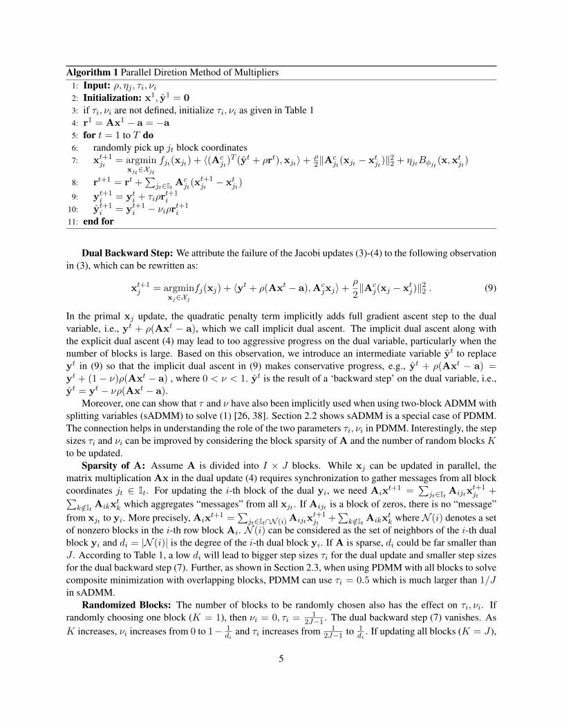
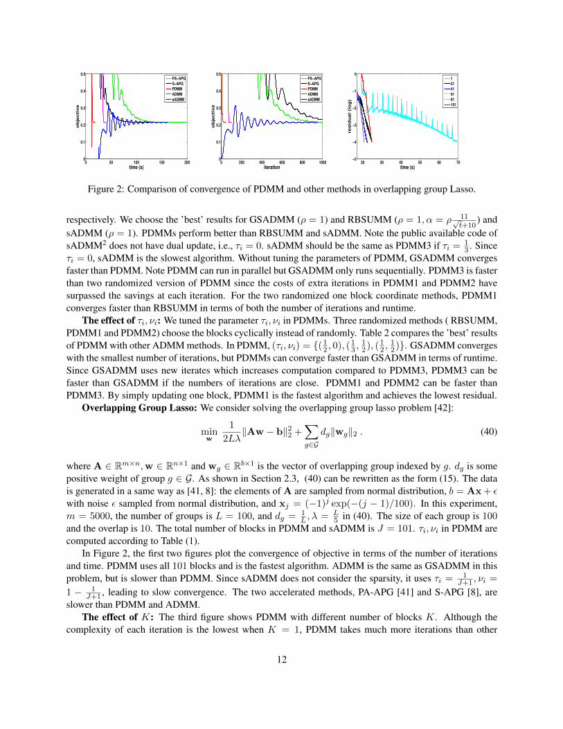
Figure 2: Comparison of convergence of PDMM and other methods in overlapping group Lasso.

respectively. We choose the ’best’ results for GSADMM (ρ = 1) and RBSUMM (ρ = 1, α = ρ 11√t+10

) andsADMM (ρ = 1). PDMMs perform better than RBSUMM and sADMM. Note the public available code ofsADMM2 does not have dual update, i.e., τi = 0. sADMM should be the same as PDMM3 if τi = 1

3 . Sinceτi = 0, sADMM is the slowest algorithm. Without tuning the parameters of PDMM, GSADMM convergesfaster than PDMM. Note PDMM can run in parallel but GSADMM only runs sequentially. PDMM3 is fasterthan two randomized version of PDMM since the costs of extra iterations in PDMM1 and PDMM2 havesurpassed the savings at each iteration. For the two randomized one block coordinate methods, PDMM1converges faster than RBSUMM in terms of both the number of iterations and runtime.

The effect of τi, νi: We tuned the parameter τi, νi in PDMMs. Three randomized methods ( RBSUMM,PDMM1 and PDMM2) choose the blocks cyclically instead of randomly. Table 2 compares the ’best’ resultsof PDMM with other ADMM methods. In PDMM, (τi, νi) = {(12 , 0), (13 ,

12), (12 ,

12)}. GSADMM converges

with the smallest number of iterations, but PDMMs can converge faster than GSADMM in terms of runtime.Since GSADMM uses new iterates which increases computation compared to PDMM3, PDMM3 can befaster than GSADMM if the numbers of iterations are close. PDMM1 and PDMM2 can be faster thanPDMM3. By simply updating one block, PDMM1 is the fastest algorithm and achieves the lowest residual.

Overlapping Group Lasso: We consider solving the overlapping group lasso problem [42]:

minw

1

2Lλ‖Aw − b‖22 +

∑g∈G

dg‖wg‖2 . (40)

where A ∈ Rm×n,w ∈ Rn×1 and wg ∈ Rb×1 is the vector of overlapping group indexed by g. dg is somepositive weight of group g ∈ G. As shown in Section 2.3, (40) can be rewritten as the form (15). The datais generated in a same way as [41, 8]: the elements of A are sampled from normal distribution, b = Ax+ εwith noise ε sampled from normal distribution, and xj = (−1)j exp(−(j − 1)/100). In this experiment,m = 5000, the number of groups is L = 100, and dg = 1

L , λ = L5 in (40). The size of each group is 100

and the overlap is 10. The total number of blocks in PDMM and sADMM is J = 101. τi, νi in PDMM arecomputed according to Table (1).

In Figure 2, the first two figures plot the convergence of objective in terms of the number of iterationsand time. PDMM uses all 101 blocks and is the fastest algorithm. ADMM is the same as GSADMM in thisproblem, but is slower than PDMM. Since sADMM does not consider the sparsity, it uses τi = 1

J+1 , νi =

1 − 1J+1 , leading to slow convergence. The two accelerated methods, PA-APG [41] and S-APG [8], are

slower than PDMM and ADMM.The effect of K: The third figure shows PDMM with different number of blocks K. Although the

complexity of each iteration is the lowest when K = 1, PDMM takes much more iterations than other

12

cases and thus takes the longest time. As K increases, PDMM converges faster and faster. When K = 20,the runtime is already same as using all blocks. When K > 21, PDMM takes less time to converge thanusing all blocks. The runtime of PDMM decreases as K increases from 21 to 61. However, the speedupfrom 61 to 81 is negligable. We tried different set of parameters for RBSUMM ρ i

2+1i+t (0 ≤ i ≤ 5, ρ =

0.01, 0.1, 1) or sufficiently small step size, but did not see the convergence of the objective within 5000iterations. Therefore, the results are not included here.

6 Conclusions

We proposed a randomized block coordinate variant of ADMM named Parallel Direction Method of Mul-tipliers (PDMM) to solve the class of problem of minimizing block-separable convex functions subject tolinear constraints. PDMM considers the sparsity and the number of blocks to be updated when setting thestep size. We show two other Jacobian ADMM methods are two special cases of PDMM. We also usePDMM to solve overlapping block problems. The global convergence and the iteration complexity are es-tablished with constant step size. Experiments on robust PCA and overlapping group lasso show that PDMMis faster than existing methods.

Acknowledgment

H. W. and A. B. acknowledge the support of NSF via IIS-0953274, IIS-1029711, IIS- 0916750, IIS-0812183and NASA grant NNX12AQ39A. H. W. acknowledges the support of DDF (2013-2014) from the Universityof Minnesota.A.B. acknowledges support from IBM and Yahoo. Z.Q. Luo is supported in part by theUS AFOSR, grant number FA9550-12-1-0340 and the National Science Foundation, grant number DMS-1015346.

References

[1] M.V. Afonso, J.M. Bioucas-Dias, and M.A.T. Figueiredo. Fast image recovery using variable splittingand constrained optimization. IEEE Transactions on Image Processing, 19(9):2345 – 2356, 2010.

[2] F. Bach, R. Jenatton, J. Mairal, and G. Obozinski. Convex Optimization with Sparsity-Inducing Norms.S. Sra, S. Nowozin, S. J. Wright., editors, Optimization for Machine Learning, MIT Press, 2011.

[3] S. Boyd, E. Chu N. Parikh, B. Peleato, and J. Eckstein. Distributed optimization and statistical learningvia the alternating direction method of multipliers. Foundation and Trends Machine Learning, 3(1):1–122, 2011.

[4] S. Boyd and L. Vandenberghe. Convex Optimization. Cambridge University Press, 2004.

[5] E. J. Candes, X. Li, Y. Ma, and J. Wright. Robust principal component analysis ?. Journal of the ACM,58:1–37, 2011.

[6] V. Chandrasekaran, P. A. Parrilo, and A. S. Willsky. Latent variable graphical model selection viaconvex optimization. Annals of Statistics, 40:1935–1967, 2012.

[7] C. Chen, B. He, Y. Ye, and X. Yuan. The direct extension of ADMM for multi-block convex mini-mization problems is not necessarily convergent. Preprint, 2013.

13

[8] X. Chen, Q. Lin, S. Kim, J. G. Carbonell, and E. P. Xing. Smoothing proximal gradient method forgeneral structured sparse regression. The Annals of Applied Statistics, 6:719752, 2012.

[9] W. Deng, M. Lai, Z. Peng, and W. Yin. Parallel multi-block admm with o(1/k) convergence. ArXiv,2014.

[10] W. Deng and W. Yin. On the global and linear convergence of the generalized alternating directionmethod of multipliers. ArXiv, 2012.

[11] M. A. T. Figueiredo and J. M. Bioucas-Dias. Restoration of poissonian images using alternatingdirection optimization. IEEE Transactions on Image Processing, 19:3133–3145, 2010.

[12] Q. Fu, H. Wang, and A. Banerjee. Bethe-ADMM for tree decomposition based parallel MAP inference.In Conference on Uncertainty in Artificial Intelligence (UAI), 2013.

[13] D. Gabay. Applications of the method of multipliers to variational inequalities. In AugmentedLagrangian Methods: Applications to the Solution of Boundary-Value Problems. M. Fortin and R.Glowinski, eds., North-Holland: Amsterdam, 1983.

[14] D. Gabay and B. Mercier. A dual algorithm for the solution of nonlinear variational problems viafinite-element approximations. Computers and Mathematics with Applications, 2:17–40, 1976.

[15] T. Goldstein, X. Bresson, and S. Osher. Geometric applications of the split Bregman method: segmen-tation and surface reconstruction. Journal of Scientific Computing, 45(1):272–293, 2010.

[16] T. Goldstein, B. Donoghue, and S. Setzer. Fast alternating direction optimization methods. CAM report12-35, UCLA, 2012.

[17] B. He, M. Tao, and X. Yuan. Alternating direction method with Gaussian back substitution for separa-ble convex programming. SIAM Journal of Optimization, pages 313–340, 2012.

[18] B. He and X. Yuan. On the O(1/n) convergence rate of the Douglas-Rachford alternating directionmethod. SIAM Journal on Numerical Analysis, 50:700–709, 2012.

[19] M. Hong, T. Chang, X. Wang, M. Razaviyayn, S. Ma, and Z. Luo. A block successive upper boundminimization method of multipliers for linearly constrained convex optimization. Preprint, 2013.

[20] M. Hong and Z. Luo. On the linear convergence of the alternating direction method of multipliers.ArXiv, 2012.

[21] S. Kasiviswanathan, H. Wang, A. Banerjee, and P. Melville. Online l1-dictionary learning with appli-cation to novel document detection. In Neural Information Processing Systems (NIPS), 2012.

[22] Z. Lin, M. Chen, L. Wu, and Y. Ma. The augmented Lagrange multiplier method for exact recovery ofcorrupted low-rank matrices. UIUC Technical Report UILU-ENG-09-2215, 2009.

[23] S. Ma, L. Xue, and H. Zou. Alternating direction methods for latent variable Gaussian graphical modelselection. Neural Computation, 25:2172–2198, 2013.

[24] Y. Nesterov. Efficiency of coordinate descent methods on huge-scale optimization methods. SIAMJournal on Optimization, 22(2):341362, 2012.

14

[25] H. Ouyang, N. He, L. Tran, and A. Gray. Stochastic alternating direction method of multipliers. InInternational Conference on Machine Learning (ICML), 2014.

[26] N. Parikh and S. Boyd. Proximal algorithms. Foundations and Trends in Optimization, 1:123–231,2014.

[27] P. Richtarik and M. Takac. Iteration complexity of randomized block-coordinate descent methods forminimizing a composite function. Mathematical Programming, 2012.

[28] R. Rockafellar. The multiplier method of hestenes and powell applied to convex programming. Journalof Optimization Theory and Applications, 12:555–562, 1973.

[29] R. Rockafellar. Augmented lagrangians and applications of the proximal point algorithm in convexprogramming. Mathematics of Operations Research, 1:97–116, 1976.

[30] K. Scheinberg, S. Ma, and D. Goldfarb. Sparse inverse covariance selection via alternating linearizationmethods. In Neural Information Processing Systems (NIPS), 2010.

[31] N. Z. Shor. Minimization Methods for Non-Differentiable Functions. Springer-Verlag, 1985.

[32] T. Suzuki. Dual averaging and proximal gradient descent for online alternating direction multipliermethod. In International Conference on Machine Learning (ICML), 2013.

[33] T. Suzuki. Stochastic dual coordinate ascent with alternating direction method of multipliers. InInternational Conference on Machine Learning (ICML), 2014.

[34] R. Tappenden, P. Richtarik, and B. Buke. Separable approximations and decomposition methods forthe augmented lagrangian. Preprint, 2013.

[35] H. Wang and A. Banerjee. Online alternating direction method. In International Conference on Ma-chine Learning (ICML), 2012.

[36] H. Wang and A. Banerjee. Bregman alternating direction method of multipliers. ArXiv, 2013.

[37] H. Wang, A. Banerjee, C. Hsieh, P. Ravikumar, and I. Dhillon. Large scale distributed sparse precesionestimation. In Neural Information Processing Systems (NIPS), 2013.

[38] X. Wang, M. Hong, S. Ma, and Z. Luo. Solving multiple-block separable convex minimization prob-lems using two-block alternating direction method of multipliers. Preprint, 2013.

[39] A. Yang, A. Ganesh, Z. Zhou, S. Sastry, and Y. Ma. Fast l1-minimization algorithms for robust facerecognition. Preprint, 2010.

[40] J. Yang and Y. Zhang. Alternating direction algorithms for L1-problems in compressive sensing. ArXiv,2009.

[41] Y. Yu. Better approximation and faster algorithm using the proximal average. In Neural InformationProcessing Systems (NIPS), 2012.

[42] P. Zhao, G. Rocha, and B. Yu. The composite absolute penalties family for grouped and hierarchicalvariable selection. Annals of Statistics, 37:34683497, 2009.

[43] Z. Zhou, X. Li, J. Wright, E. Candes, and Y. Ma. Stable principal component pursuit. In IEEEInternational Symposium on Information Theory, 2010.

15

A Convergence Analysis

A.1 Technical Preliminaries

We first define some notations will be used specifically in this section. Let zij = Aijxj ∈ Rmi×1, zri =[zTi1, · · · , zTiJ ]T ∈ RmiJ×1 and z = [(zr1)

T , · · · , (zrI)T ]T ∈ RJm×1. Let Wi ∈ RJmi×mi be a columnvector of Wij ∈ Rmi×mi where

Wij =

{Imi , if Aij 6= 0 ,0 otherwise .

(41)

Define Q ∈ RJm×Jm as a diagonal matrix of Qi ∈ RJmi×Jmi and

Q = diag([Q1, · · · ,QI ]) ,Qi = diag(Wi)−1

diWiW

Ti . (42)

Therefore, for an optimal solution x∗ satisfying Ax∗ = a, we have

‖zt − z∗‖2Q =I∑i=1

‖zti − z∗i ‖2Qi=

I∑i=1

‖zti − z∗i ‖2diag(wi)− 1di

wiwTi

=I∑i=1

∑j∈N (i)

‖ztij − z∗ij‖22 −1

di‖wT

i (zti − z∗i )‖22

=

I∑i=1

[‖zti − z∗i ‖22 −

1

di‖Ar

ixt − ai‖22

], (43)

where the last equality uses wTi z∗i = Ar

ix∗ = ai.

In the following lemma, we prove that Qi is a positive semi-definite matrix. Thus, Q is also positivesemi-definite.

Lemma 3 Qi is positive semi-definite.

Proof: As Wij is either an identity matrix or a zero matrix, Wi has di nonzero entries. Removing the zeroentries from Wi, we have Wi which only has di nonzero entries. Then,

Wi =

Imi

...Imi

, diag(Wi) =

Imi

. . .Imi

, (44)

diag(Wi) is an identity matrix. Define Qi = diag(Wi)− 1diWiW

Ti . If Qi is positive semi-definite, Qi is

positive semi-definite.Denote λmax

Wias the largest eigenvalue of WiW

Ti , which is equivalent to the largest eigenvalue of

WTi Wi. Since WT

i Wi = diImi , then λmaxWi

= di. Then, for any v,

‖v‖2WiWT

i≤ λmax

Wi‖v‖22 = di‖v‖22 . (45)

16

Thus,

‖v‖2Qi= ‖v‖2diag(Wi)− 1

diWiWT

i= ‖v‖22 −

1

di‖v‖2

WiWTi≥ 0 , (46)

which completes the proof.

Let Wti ∈ RJmi×mi be a column vector of Wijt ∈ Rmi×mi where

Wijt =

{Imi , if Aijt 6= 0 and jt ∈ It ,0 otherwise .

(47)

Define Pt ∈ RJm×Jm as a diagonal matrix of Pti ∈ RJmi×Jmi and

Pt = diag[Pt1, · · · ,Pt

I ] ,Pti = diag(Wt

i)−1

Ki

Wti(W

ti)T . (48)

where Ki = min{K, di} ≥ min{|It ∩ Ni|, di}. Using similar arguments in Lemma 3, we can show Pt ispositive semi-definite. Therefore,

‖zt+1 − zt‖2Pt=

I∑i=1

‖zt+1i − zti‖2Pt

i=

I∑i=1

‖zt+1i − zti‖2diag(wt

i)−1Ki

wti(w

ti)

T

=I∑i=1

∑jt∈It

‖zt+1ijt− ztijt‖

22 −

1

Ki

‖(wti)T (zt+1

i − zti)‖22

=

I∑i=1

[‖zt+1i − zti‖22 −

1

Ki

‖Ari (x

t+1 − xt)‖22]. (49)

In PDMM, an index set It is randomly chosen. Conditioned on xt, xt+1 and yt+1 depend on It. Pt

depends on It. xt,yt are independent of It. xt depends on a sequence of observed realization of randomvariable

ξt−1 = {I1, I2, · · · , It−1} . (50)

As we do not assume that fjt is differentiable, we use the subgradient of fjt . In particular, if fjt isdifferentiable, the subgradient of fjt becomes the gradient, i.e.,∇fjt(xjt). PDMM (5)-(7) has the followinglemma.

17

Lemma 4 Let {xtjt ,yti} be generated by PDMM (5)-(7). Assume τi > 0 and νi ≥ 0. We have

∑jt∈It

fjt(xt+1jt

)− fjt(x∗jt) ≤ −K

J

I∑i=1

{〈yti,Ar

ixt − ai〉 −

τiρ

2‖Ar

ixt − ai‖22

}−∑jt∈It

〈yt + ρ(Axt − a),Acjt(x

tjt − x∗jt)〉+

K

J〈yt + ρ(Axt − a),Axt − a〉

+I∑i=1

{〈yti,Ar

ixt − ai〉 −

τiρ

2‖Ar

ixt − ai‖22

}−

I∑i=1

{〈yt+1i ,Ar

ixt+1 − ai〉 −

τiρ

2‖Ar

ixt+1 − ai‖22

}+ρ

2(‖z∗ − zt‖2Q − ‖z∗ − zt+1‖2Q − ‖zt+1 − zt‖2Pt

)

+∑jt∈It

ηjt(Bφjt (x∗jt ,x

tjt)−Bφjt (x

∗jt ,x

t+1jt

)−Bφjt (xt+1jt

,xtjt))

+ρ

2

I∑i=1

{[(1− 2K

J)(1− νi) + (1− K

J)τi +

1

di]‖Ar

ixt − ai‖22 − (1− νi − τi +

1

di)‖Ar

ixt+1 − ai‖22

+ (1− νi −1

Ki

)‖Ari (x

t+1 − xt)‖22}. (51)

Proof: Let ∂fjt(xt+1jt

) be the subdifferential of fjt at xt+1jt

. The optimality of the xjt update (5) is

0 ∈ ∂fjt(xt+1jt

) + (Acjt)

T [yt + ρ(Acjtx

t+1jt

+∑k 6=jt

Ackx

tk − a)] + ηjt(∇φjt(xt+1

jt)−∇φjt(xtjt)) , (52)

Using (7) and rearranging the terms yield

− (Acjt)

T [yt + ρ(Axt − a) + ρAcjt(x

t+1jt− xtjt)] + ηjt(∇φjt(xt+1

jt)−∇φjt(xtjt)) ∈ ∂fjt(x

t+1jt

) . (53)

Using the convexity of fjt , we have

fjt(xt+1jt

)− fjt(x∗jt) ≤ −〈yt + ρ(Axt − a),Ac

jt(xt+1jt− x∗jt)〉

− ρ〈Acjt(x

t+1jt− xtjt),A

cjt(x

t+1jt− x∗jt)〉 − ηjt〈∇φjt(x

t+1jt

)−∇φjt(xtjt),xt+1jt− x∗jt〉

= −〈yt + ρ(Axt − a),Acjt(x

tjt − x∗jt)〉 − 〈y

t + ρ(Axt − a),Acjt(x

t+1jt− xtjt)〉

− ρI∑i=1

〈Aijt(xt+1jt− xtjt),Aijt(x

t+1jt− x∗jt)〉

+ ηjt

(Bφjt (x

∗jt ,x

tjt)−Bφjt (x

∗jt ,x

t+1jt

)−Bφjt (xt+1jt

,xtjt)). (54)

18

Summing over jt ∈ It, we have∑jt∈It

fjt(xt+1jt

)− fjt(x∗jt)

≤ −∑jt∈It


tjt − x∗jt)〉 − 〈y

t + ρ(Axt − a),∑jt∈It

Acjt(x

t+1jt− xtjt)〉

− ρI∑i=1

∑jt∈It

〈Aijt(xt+1jt− xtjt),Aijt(x

t+1jt− x∗jt)〉

+∑jt∈It

ηjt

(Bφjt (x

∗jt ,x

tjt)−Bφjt (x

∗jt ,x

t+1jt

)−Bφjt (xt+1jt

,xtjt))

= −∑jt∈It


tjt − x∗jt)〉+

K


−KJ〈yt + ρ(Axt − a),Axt − a〉 − 〈yt + ρ(Axt − a),A(xt+1 − xt)〉︸︷︷︸

H1

+ρ

2

I∑i=1

∑jt∈It

(‖Aijt(x∗jt − xtjt)‖

22 − ‖Aijt(x

∗jt − xt+1

jt)‖22 − ‖Aijt(x

t+1jt− xtjt)‖

22)︸︷︷︸

H2

+∑jt∈It

ηjt

(Bφjt (x

∗jt ,x

tjt)−Bφjt (x

∗jt ,x

t+1jt

)−Bφjt (xt+1jt

,xtjt)). (55)

H1 in (55) can be rewritten as

H1 = −〈yt + ρ(Axt − a),Axt+1 − a〉+ (1− K

J)〈yt + ρ(Axt − a),Axt − a〉 . (56)

19

The first term of (56) is equivalent to

− 〈yt + ρ(Axt − a),Axt+1 − a〉

= −I∑i=1

〈yti + ρ(Arix

t − ai),Arix

t+1 − ai〉

= −I∑i=1

〈yti + (1− νi)ρ(Arix

t − ai),Arix

t+1 − ai〉

= −I∑i=1

{〈yt+1i − τiρ(Ar

ixt+1 − ai),A

rix

t+1 − ai〉+ (1− νi)ρ〈Arix

t − ai,Arix

t+1 − ai〉}

= −I∑i=1

{〈yt+1i ,Ar

ixt+1 − ai〉 − τiρ‖Ar

ixt+1 − ai‖22

−(1− νi)ρ2

(‖Ari (x

t+1 − xt)‖22 − ‖Arix

t − ai‖22 − ‖Arix

t+1 − ai‖22)}

= −I∑i=1

{〈yt+1i ,Ar

ixt+1 − ai〉 −

τiρ

2‖Ar

ixt+1 − ai‖22

}+

I∑i=1

{(1− νi)ρ

2(‖Ar

i (xt+1 − xt)‖22 − ‖Ar

ixt − ai‖22)−

(1− νi − τi)ρ2

‖Arix

t+1 − ai‖22}. (57)

The second term of (56) is equivalent to

(1− K

J)〈yt + ρ(Axt − a),Axt − a〉

= (1− K

J)

I∑i=1

〈yti + ρ(Arix

t − ai),Arix

t − ai〉

= (1− K

J)

I∑i=1

〈yti + (1− νi)ρ(Arix

t − ai),Arix

t − ai〉

= (1− K

J)

I∑i=1

{〈yti,Ar

ixt − ai〉 −

τiρ

2‖Ar

ixt − ai‖22

}+ (1− K

J)

I∑i=1

(1− νi +τi2

)ρ‖Arix

t − ai‖22 .

(58)

20

H2 in (55) is equavilant to

H2 =ρ

2

I∑i=1

∑jt∈It

(‖z∗ijt − ztijt‖22 − ‖z∗ijt − zt+1

ijt‖22 − ‖zt+1

ijt− ztijt‖

22)

=ρ

2

I∑i=1

(‖z∗i − zti‖22 − ‖z∗i − zt+1i ‖

22 − ‖zt+1

i − zti‖22)

=ρ

2(‖z∗ − zt‖2Q − ‖z∗ − zt+1‖2Q − ‖zt+1 − zt‖2Pt

)

+ρ

2

I∑i=1

1

di(‖Ar

ixt − ai‖22 − ‖Ar

ixt+1 − ai‖22)−

1

Ki

‖Ari (x

t+1 − xt)‖22 . (59)

where the last equality uses the definition of Q in (42) and Pt (48), and Ki = min{K, di}. Combining theresults of (56)-(59) gives

H1 +H2 = −I∑i=1

{〈yt+1i ,Ar

ixt+1 − ai〉 −

τiρ

2‖Ar

ixt+1 − ai‖22

}+

I∑i=1

{(1− νi)ρ

2(‖Ar

i (xt+1 − xt)‖22 − ‖Ar

ixt − ai‖22)−

(1− νi − τi)ρ2

‖Arix

t+1 − ai‖22}

+ (1− K

J)

I∑i=1

{〈yti,Ar

ixt − ai〉 −

τiρ

2‖Ar

ixt − ai‖22

}+ (1− K

J)

I∑i=1

(1− νi +τi2

)ρ‖Arix

t − ai‖22

+ρ

2(‖z∗ − zt‖2Q − ‖z∗ − zt+1‖2Q − ‖zt+1 − zt‖2Pt

)

+ρ

2

I∑i=1

1

di(‖Ar


ixt+1 − ai‖22)−

1

Ki

‖Ari (x

t+1 − xt)‖22)

= −KJ

I∑i=1

{〈yti,Ar

ixt − ai〉 −

τiρ

2‖Ar

ixt − ai‖22

}+

I∑i=1

{〈yti,Ar

ixt − ai〉 −

τiρ

2‖Ar

ixt − ai‖22

}−

I∑i=1

{〈yt+1i ,Ar

ixt+1 − ai〉 −

τiρ

2‖Ar

ixt+1 − ai‖22

}+ρ

2(‖z∗ − zt‖2Q − ‖z∗ − zt+1‖2Q − ‖zt+1 − zt‖2Pt

)

+ρ

2

I∑i=1

{[(1− 2K

J)(1− νi) + (1− K

J)τi +

1

di]‖Ar

ixt − ai‖22 − (1− νi − τi +

1

di)‖Ar

ixt+1 − ai‖22

+ (1− νi −1

Ki

)‖Ari (x

t+1 − xt)‖22}. (60)

Plugging back into (55) completes the proof.

21

Lemma 5 Let {xtjt ,yti} be generated by PDMM (5)-(7). Assume τi > 0 and νi ≥ 0. We have

∑jt∈It

fjt(xt+1jt

)− fjt(x∗jt) ≤ −K

J

I∑i=1

{〈yti,Ar

ixt − ai〉 −

τiρ

2‖Ar

ixt − ai‖22

}−∑jt∈It


tjt − x∗jt)〉+

K


+

I∑i=1

{〈yti,Ar

ixt − ai〉 −

τiρ

2‖Ar

ixt − ai‖22

}−

I∑i=1

{〈yt+1i ,Ar

ixt+1 − ai〉 −

τiρ

2‖Ar

ixt+1 − ai‖22

}+ρ

2(‖z∗ − zt‖2Q − ‖z∗ − zt+1‖2Q − ‖zt+1 − zt‖2Pt

)

+ ηT (Bφ(x∗,xt)−Bφ(x∗,xt+1)−Bφ(xt+1,xt))

+ρ

2

I∑i=1

[γi(‖Ar


ixt+1 − ai‖22)− βi‖Ar

ixt+1 − ai‖22

]. (61)

where ηT = [η1, · · · , ηJ ]. τi > 0, νi ≥ 0, γi ≥ 0 and βi ≥ 0 satisfy the following conditions:

νi ∈ (max{0, 1− 2J

Ki(2J −K)}, 1− 1

Ki

] , (62)

τi ≤J

2J −K[

4

Ki

− (4− 2K

J)(1− νi)] ≤

2K

Ki(2J −K), (63)

γi = (3− 2K

J)(1− νi) + (1− K

J)τi +

1

di− 2

Ki

, (64)

βi =4

Ki

− (2− K

J)[2(1− νi) + τi] . (65)

Proof: In (51), denote

H3 = [(1− 2K

J)(1− νi) + (1− K

J)τi +

1

di]‖Ar

ixt − ai‖22 − (1− νi − τi +

1

di)‖Ar

ixt+1 − ai‖22 ,

(66)

H4 = (1− νi −1

Ki

)‖Ari (x

t+1 − xt)‖22 . (67)

Our goal is to eliminate H4 so that

H3 +H4 = γi(‖Arix


t+1 − ai‖22)− βi‖Arix

t+1 − ai‖22 , (68)

where γi ≥ 0 and βi ≥ 0 .We want to choose a large τi and a small νi. Assume 1− νi − 1

Ki≥ 0, i.e., νi ≤ 1− 1

Ki, we have

H4 = (1− νi −1

Ki

)‖Ari (x

t+1 − xt)‖22 ≤ 2(1− νi −1

Ki

)(‖Arix

t − ai‖22 + ‖Arix

t+1 − ai‖22) . (69)

Therefore, we have

H3 +H4 ≤ [(3− 2K

J)(1− νi) + (1− K

J)τi +

1

di− 2

Ki

]‖Arix

t − ai‖22 + (1− νi + τi −1

di− 2

Ki

)‖Arix

t+1 − ai‖22

= γi(‖Arix


t+1 − ai‖22)− βi‖Arix

t+1 − ai‖22 . (70)

22

where

γi = (3− 2K

J)(1− νi) + (1− K

J)τi +

1

di− 2

Ki

≥ (3− 2K

J)

1

Ki

+ (1− K

J)τi +

1

di− 2

Ki

= (1− K

J)

1

Ki

− K

JKi

+1

di+ (1− K

J)τi ≥ 0 . (71)

and

βi = −(1− νi + τi −1

di− 2

Ki

+ γi) =4

Ki

− (2− K

J)[2(1− νi) + τi] . (72)

We also want βi ≥ 0, which can be reduced to

τi ≤J

2J −K[

4

Ki

− (4− 2K

J)(1− νi)] (73)

≤ J

2J −K[

4

Ki

− (4− 2K

J)

1

Ki

]

=2K

Ki(2J −K).

It also requires the RHS of (73) to be positive, leading to νi > max{0, 1 − 2JKi(2J−K)

}. Therefore, νi ∈(max{0, 1− 2J

Ki(2J−K)}, 1− 1

Ki].

Denote Bφ = [Bφ1 , · · · , BφJ]T as a column vector of the Bregman divergence on block coordi-

nates of x. Using xt+1 = [xt+1jt∈It ,x

tjt 6∈It ]

T , we have Bφjt (x∗jt,xtjt) − Bφjt (x

∗jt,xt+1

jt) = Bφ(x∗,xt) −

Bφ(x∗,xt+1), Bφjt (xt+1jt

,xtjt) = Bφ(xt+1,xt). Thus,∑jt∈It

ηjt

(Bφjt (x

∗jt ,x

tjt)−Bφjt (x

∗jt ,x

t+1jt

)−Bφjt (xt+1jt

,xtjt))

= ηT (Bφ(x∗,xt)−Bφ(x∗,xt+1)−Bφ(xt+1,xt)) . (74)

where ηT = [η1, · · · , ηJ ].

Lemma 6 Let {xtjt ,yti} be generated by PDMM (5)-(7). Assume τi > 0 and νi ≥ 0 satisfy the conditions

in Lemma 5. We have

f(xt)− f(x∗) ≤ −I∑i=1

{〈yti,Ar

ixt − ai〉 −

τiρ

2‖Ar

ixt − ai‖22

}+J

K

{Lρ(xt,yt)− EItLρ(xt+1,yt+1)− ρ

2

I∑i=1

βiEIt‖Arix

t+1 − ai‖22

+ρ

2(‖z∗ − zt‖2Q − EIt‖z∗ − zt+1‖2Q − EIt‖zt+1 − zt‖2Pt

)

+ ηT (Bφ(x∗,xt)− EItBφ(x∗,xt+1)− EItBφ(xt+1,xt))

}. (75)

23

where Lρ is defined as follows:

Lρ(xt,yt) = f(xt)− f(x∗) +I∑i=1

{〈yti,Ar

ixt − ai〉+

(γi − τi)ρ2

‖Arix

t − ai‖22}. (76)

τi, νi, γi, βi and η are defined in Lemma 5.

Proof: Using xt+1 = [xt+1jt∈It ,x

tjt 6∈It ]

T , we have

f(xt+1)− f(xt) =∑jt∈It

fjt(xt+1jt

)− fjt(xtjt) =∑jt∈It

[fjt(xt+1jt

)− fjt(x∗jt)]−∑jt∈It

[fjt(xtjt)− fjt(x

∗jt)] .

(77)

Rearranging the terms and using Lemma 5 yield∑jt∈It

fjt(xtjt)− fjt(x

∗jt) =

∑j∈It

[fjt(xt+1jt

)− fjt(x∗jt)] + f(xt)− f(xt+1)

≤ −KJ

I∑i=1

{〈yti,Ar

ixt − ai〉 −

τiρ

2‖Ar

ixt − ai‖22

}−∑jt∈It


tjt − x∗jt)〉+

K


+ Lρ(xt,yt)− Lρ(xt+1,yt+1)− ρ

2

I∑i=1

βi‖Arix

t+1 − ai‖22

+ρ

2(‖z∗ − zt‖2Q − ‖z∗ − zt+1‖2Q − ‖zt+1 − zt‖2Pt

)

+ ηT (Bφ(x∗,xt)−Bφ(x∗,xt+1)−Bφ(xt+1,xt)) , (78)

where Lρ(xt,yt) is defined in (76). Conditioning on xt and taking expectation over It, we have

K

J[f(xt)− f(x∗)] ≤ −K

J

I∑i=1

{〈yti,Ar

ixt − ai〉 −

τiρ

2‖Ar

ixt − ai‖22

}+ Lρ(xt,yt)− EItLρ(xt+1,yt+1)− ρ

2

I∑i=1

βiEIt‖Arix

t+1 − ai‖22

+ρ


)

+ ηT (Bφ(x∗,xt)− EItBφ(x∗,xt+1)− EItBφ(xt+1,xt)) , (79)

where we use

EIt [−∑jt∈It


tjt − x∗jt)〉] = −K

J〈yt + ρ(Axt − a),Axt − a〉 . (80)

Dividing both sides by KJ and using the definition (76) complete the proof.

24

A.2 Theoretical Results

We establish the convergence results for PDMM under fairly simple assumptions:

Assumption 2(1) fj : Rnj → R ∪ {+∞} are closed, proper, and convex.(2) A KKT point of the Lagrangian (ρ = 0 in (2)) of Problem (1) exists.

Assumption 2 is the same as that required by ADMM [3, 35]. Let ∂fj be the subdifferential of fj .Assume that {x∗j ,y∗i } satisfies the KKT conditions of the Lagrangian (ρ = 0 in (2)), i.e.,

−ATj y∗ ∈ ∂fj(x∗j ) , (81)

Ax∗ − a = 0. (82)

During iterations, (82) is satisfied if Axt+1 = a. The optimality conditions for the xj update (5) is

0 ∈ ∂fj(xt+1j ) + Ac

j [yt + ρ(Ac

jxt+1j +

∑k 6=j

Ackx

tk − a)] + ηj(∇φj(xt+1

j )−∇φj(xtj)) , (83)

which is equivalent to

−Acj [y

t + (1− ν)ρ(Axt − a) + Acj(x

t+1j − xtj)]− ηj(∇φj(xt+1

j )−∇φj(xtj)) ∈ ∂fj(xt+1j ) . (84)

When Axt+1 = a, yt+1 = yt. If Acj(x

t+1j − xtj) = 0, then Axt − a = 0. When ηj ≥ 0, further

assuming Bφj (xt+1j ,xtj) = 0, (81) will be satisfied. Overall, the KKT conditions (81)-(82) are satisfied if

the following optimality conditions are satisfied by the iterates:

Axt+1 = a ,Acj(x

t+1j − xtj) = 0 , (85)

Bφj (xt+1j ,xtj) = 0 . (86)

The above optimality conditions are sufficient for the KKT conditions. (85) are the optimality conditions forthe exact PDMM. (86) is needed only when ηj > 0.

In Lemma 5, setting the values of νi, τi, γi, βi as follows:

νi = 1− 1

Ki

, τi =K

Ki(2J −K), γi =

2(J −K)

Ki(2J −K)+

1

di− K

JKi

, βi =K

JKi

. (87)

Define the residual of optimality conditions (85)-(86) as

R(xt+1) =ρ

2‖zt+1 − zt‖2Pt

+ρ

2

I∑i=1

βi‖Arix

t+1 − ai‖22 + [ηTBφ(xt+1,xt)] . (88)

If R(xt+1)→ 0, (85)-(86) will be satisfied and thus PDMM converges to the KKT point {x∗,y∗}.Define the current iterate vt = (xtj ,y

ti) and h(v∗,vt) as a distance from vt to a KKT point v∗ =

(x∗j ,y∗i ):

h(v∗,vt) =K

J

I∑i=1

1

2τiρ‖y∗i − yt−1i ‖

22 + Lρ(xt,yt) +

ρ

2‖z∗ − zt‖2Q + ηTBφ(x∗,xt) . (89)


25

Lemma 7 Let h(v∗,vt) be defined in (89). Setting νi = 1− 1Ki


, we have

h(v∗,vt) ≥ ρ

2

I∑i=1

ζi‖Arix

t − ai‖22 +ρ

2‖z∗ − zt‖2Q + +

J∑j=1

ηjBφj (x∗j ,x

tj) ≥ 0 . (90)

where ζi = J−KKi(2J−K)

+ 1di− K


ixt = ai, z

t = z∗ and

Bφj (x∗j ,x


Proof: Using the convexity of f and (81), we have

f(x∗)− f(xt) ≤ −〈ATy∗,x∗ − xt〉 =

I∑i=1

〈y∗i ,Arix

t − ai〉 . (91)

Thus,

Lρ(xt,yt) = f(xt)− f(x∗) +

I∑i=1

{〈yti,Ar

ixt − ai〉+

(γi − τi)ρ2

‖Arix

t − ai‖22}

≥I∑i=1

{〈yti − y∗i ,A

rix

t − ai〉+(γi − τi)ρ

2‖Ar

ixt − ai‖22

}

=I∑i=1

{〈yt−1i − y∗i ,Aix

t − ai〉+ 〈yti − yt−1i ,Aixt − ai〉+

(γi − τi)ρ2

‖Arix

t − ai‖22}

≥I∑i=1

[− K

2Jτiρ‖yt−1i − y∗i ‖22 −

Jτiρ

2K‖Aix

t − ai‖22 +(γi + τi)ρ

2‖Aix

t − ai‖22]

=

I∑i=1

[− K

2Jτiρ‖yt−1i − y∗i ‖22 + [γi + (1− J

K)τi]

ρ

2‖Aix

t − ai‖22]. (92)

h(v∗,vt) is reduced to

h(v∗,vt) ≥ ρ

2

I∑i=1

[γi + (1− J

K)τi]‖Aix

t − ai‖22 +ρ

2‖z∗ − zt‖2Q + ηTBφ(x∗,xt) . (93)

Setting 1− νi = 1Ki


, we have

γi + (1− J

K)τi = (3− 2K

J)(1− νi) + (1− K

J)τi +

1

di− 2

Ki

+ (1− J

K)τi

= (1− K

J)

1

Ki

+ (2− K

J− J

K)

K

Ki(2J −K)+

1

di− K

JKi

=(J −K)

Ki(2J −K)+

1

di− K

JKi

≥ 0 . (94)

Therefore, h(v∗,vt) ≥ 0. Letting ζi = J−KKi(2J−K)

+ 1di− K

JKicompletes the proof.


26

Theorem 5 (Global Convergence of PDMM) Let vt = (xtjt ,yti) be generated by PDMM (5)-(7) and v∗ =

(x∗j ,y∗i ) be a KKT point satisfying (81)-(82). Setting νi = 1− 1

Kiand τi = K

Ki(2J−K), we have


Proof: Adding (91) and (75) yields

0 ≤I∑i=1

{〈y∗i − yti,A

rix

t − ai〉+τiρ

2‖Ar

ixt − ai‖22

}+J

K


2

I∑i=1

βiEIt‖Arix

t+1 − ai‖22

+ρ


)


}. (96)

Using (6), we have

〈y∗i − yti,Arix

t − ai〉+τiρ

2‖Ar

ixt − ai‖22 =

1

τiρ〈y∗i − yti,y

ti − yt−1i 〉+

τiρ

2‖Ar

ixt − ai‖22

=1

2τiρ(‖y∗i − yt−1i ‖

22 − ‖y∗i − yti‖22) . (97)

Plugging back into (96) gives

0 ≤I∑i=1

1

2τiρ(‖y∗i − yt−1i ‖

22 − ‖y∗i − yti‖22)

+J

K


2

I∑i=1

βiEIt‖Arix

t+1 − ai‖22

+ρ


)


}

=J

K

{h(v∗,vt)− EIth(v∗,vt+1)− EItR(xt+1)

}. (98)

Taking expectaion over ξt−1, we have

0 ≤ J

K

{Eξt−1h(v∗,vt)− Eξth(v∗,vt+1)− EξtR(xt+1)

}. (99)

Since EξtR(xt+1) ≥ 0, we have

Eξth(v∗,vt+1) ≤ Eξt−1h(v∗,vt) . (100)

Thus, Eξth(v∗,vt+1) converges monotonically.

27

Rearranging the terms in (99) yields

EξtR(xt+1) ≤ Eξt−1h(v∗,vt)− Eξth(v∗,vt+1) . (101)

Summing over t gives

T−1∑t=0

EξtR(xt+1) ≤ h(v∗,v0)− EξT−1h(v∗,vT ) ≤ h(v∗,v0) . (102)

where the last inequality uses the Lemma 7. As T →∞, EξtR(xt+1)→ 0, which completes the proof.

The following theorem establishes the iteration complexity of PDMM in an ergodic sense.

Theorem 6 Let (xtj ,yti) be generated by PDMM (5)-(7). Let xT =

∑Tt=1 x

t. Setting νi = 1 − 1Ki

and

τi = KKi(2J−K)

, we have

Ef(xT )− f(x∗) ≤

∑Ii=1

12τiρ‖y0

i ‖22 + JK

{1

2βiρ‖y∗i ‖22 + Lρ(x1,y1) + ρ

2‖z∗ − z1‖2Q + ηTBφ(x∗,x1)

}T

,

(103)

EI∑i=1

βi‖Ari x

T − ai‖22 ≤2ρh(v∗,v0)

T. (104)

where βi = KJKi

.

Proof: Using (7), we have

−I∑i=1

{〈yti,Ar

ixt − ai〉 −

τiρ

2‖Ar

ixt − ai‖22

}= −

I∑i=1

{1

τiρ〈yti,yti − yt−1i 〉 −

1

2τiρ‖yti − yt−1i ‖

22

}

=

I∑i=1

1

2τiρ(‖yt−1i ‖ − ‖y

ti‖22) . (105)

Plugging back into (75) yields

f(xt)− f(x∗) ≤I∑i=1

1

2τiρ(‖yt−1i ‖

22 − ‖yti‖22)

+J

K


2

I∑i=1

βiEIt‖Arix

t+1 − ai‖22

+ρ


)


}. (106)

28

Taking expectaion over ξt−1, we have

Eξt−1f(xt)− f(x∗) ≤I∑i=1

1

2τiρ(Eξt−2‖y

t−1i ‖

22 − Eξt−1‖yti‖22)

+J

K

{Eξt−1Lρ(xt,yt)− EξtLρ(xt+1,yt+1)− ρ

2

I∑i=1

βiEξt‖Arix

t+1 − ai‖22

+ρ

2(Eξt−1‖z∗ − zt‖2Q − Eξt‖z∗ − zt+1‖2Q − Eξt‖zt+1 − zt‖2Pt

)

+ ηT (Eξt−1Bφ(x∗,xt)− EξtBφ(x∗,xt+1)− EξtBφ(xt+1,xt))

}. (107)

Summing over t, we haveT∑t=1


1

2τiρ(‖y0

i ‖22 − EξT−1‖yTi ‖22)

+J

K

{Lρ(x1,y1)− EξT Lρ(x

T+1,yT+1)− ρ

2

T∑t=1

I∑i=1

βiEξt‖Arix

t+1 − ai‖22

+ρ

2(‖z∗ − z1‖2Q − EξT ‖z

∗ − zT+1‖2Q − EξT ‖zT+1 − zT ‖2Q)

+ ηT (Bφ(x∗,x1)− EξTBφ(x∗,xT+1)− EξTBφ(xT+1,xT ))

}. (108)

Using (91), we have

Lρ(xT+1,yT+1) = f(xT+1)− f(x∗) +I∑i=1

[〈yT+1i ,Aix

T+1 − ai〉+(γi − τi)ρ

2‖Aix

T+1 − ai‖22]

≥ −I∑i=1

〈y∗i ,Arix

T+1 − ai〉+I∑i=1

[〈yTi ,AixT+1 − ai〉+

(γi + τi)ρ

2‖Aix

T+1 − ai‖22]

≥ −I∑i=1

(1

2δi‖y∗i ‖22 +

δi2‖Ar

ixT+1 − ai‖22) +

I∑i=1

[− K

2Jτiρ‖yTi ‖22 + [γi + (1− J

K)τi]

ρ

2‖Aix

T+1 − ai‖22]

≥ −I∑i=1

(1

2δi‖y∗i ‖22 +

δi2‖Ar

ixT+1 − ai‖22)−

I∑i=1

K

2Jτiρ‖yTi ‖22 , (109)

where δi > 0 and the last inequality uses (94). Plugging into (108), we haveT∑t=1


1

2τiρ‖y0

i ‖22 +J

K

{Lρ(x1,y1) +

ρ

2‖z∗ − z1‖2Q + ηTBφ(x∗,x1)

}+J

K

{I∑i=1

[1

2δi‖y∗i ‖22 +

δi − βiρ2

E‖Arix

T+1 − ai‖22]}

. (110)

Settin δi = βiρ, dividing by T and letting xT = 1T

∑Tt=1 x

t complete the proof.Dividing both sides of (102) by T yields (104).

29

B Connection to ADMM

We use ADMM to solve (1), similar as [38, 26] but with different forms. We show that ADMM is aspeical case of PDMM. The connection can help us understand why the two parameters τi, νi in PDMM arenecessary. We first introduce splitting variables zi as follows:

min

J∑j=1

fj(xj) s.t. Ajxj = zj ,

J∑j=1

zj = a , (111)

which can be written as

min

K∑j=1

fj(xj) + g(z) s.t. Ajxj = zj , (112)

where g(z) is an indicator function of∑K

j=1 zj = a. The augmented Lagrangian is

Lρ(xj , zj ,yj) =

J∑j=1

[fj(xj) + 〈yj ,Ajxj − zj〉+

ρ

2‖Ajxj − zj‖22

], (113)

where yj is the dual variable. We have the following ADMM iterates:

xt+1j = argminxi

fj(xj) + 〈ytj ,Ajxj − ztj〉+ρ

2‖Ajxj − ztj‖22 , (114)

zt+1 = argmin∑Kj=1 zj=a

K∑j=1

[〈yti,Ajx

t+1j − zj〉+

ρ

2‖Ajx

t+1j − zj‖22

], (115)

yt+1j = ytj + ρ(Ajx

t+1j − zt+1

j ) . (116)

The Lagrangian of (115) is

L =J∑j=1

[〈ytj ,Ajx

t+1j − zj〉+

ρ

2‖Ajx

t+1j − zj‖22

]+ 〈λ,

J∑j=1

zj − a〉 , (117)

where λ is the dual variable. The first order optimality is

−ytj + ρ(zt+1j −Ajx

t+1j ) + λ = 0 . (118)

Using (116) gives

λ = yt+1j , ∀j . (119)

Denoting yt = ytj , (118) becomes

yt+1 = yt + ρ(Ajxt+1j − zt+1

j ) . (120)

Summing over j and using the constraint∑J

j=1 zi = a, we have

yt+1 = yt +ρ

J(Axt+1 − a) . (121)

30

Subtracting (120) from (121), simple calculations yields

zt+1j = Ajx

t+1j +

1

J(Axt+1 − a) . (122)

Plugging back int (114), we have

xt+1j = argminxj

fj(xj) + 〈yt,Ajxj〉+ρ

2‖Ajxj − ztj‖22

= argminxjfj(xj) + 〈yt,Ajxj〉+

ρ

2‖Ajxj −Ajx

tj +

Axt − a

J‖22

= argminxjfj(xj) + 〈yt,Ajxj〉+

ρ

2‖Ajxj +

∑k 6=j

Akxtk − a‖22 , (123)

where yt = yt − (1 − 1J )ρ(Axt − a), which becomes PDMM by setting τ = 1

J , ν = 1 − 1J and updating

all blocks. Therefore, sADMM is a special case of PDMM.

C Connection to PJADMM

We consider the case when all blocks are used in PDMM. We show that if setting ηj sufficiently large, thedual backward step (7) is not needed, which becomes PJADMM [9].

Corollary 1 Let {xtj ,yti} be generated by PDMM (5)-(7). Assume τi > 0 and νi ≥ 0. We have

f(xt+1)− f(x∗) ≤I∑i=1

{−〈yt+1

i ,Arix

t+1 − ai〉+τiρ

2‖Ar

ixt+1 − ai‖22

}+ρ

2(‖zt − z∗‖2Q − ‖zt+1 − z∗‖2Q − ‖zt+1 − zt‖2Q)

+ρ

2

I∑i=1

{(νi − 1 +

1

di)(‖Ar


ixt+1 − ai‖22)

+(τi + 2νi − 2)‖Arix

t+1 − ai‖22 + (1− νi −1

di)‖Ar

i (xt+1 − xt)‖22

}+

J∑j=1

ηj

(Bφj (x

∗j ,x

tj)−Bφj (x

∗j ,x

t+1j )−Bφj (x

t+1j ,xtj)

). (124)

31

Proof: Let It be all blocks, K = J . According the definition of Pt in (42) and Q in (48), Pt = Q.Therefore, (51) reduces to

f(xt+1)− f(x∗) ≤I∑i=1

{−〈yt+1

i ,Arix

t+1 − ai〉+τiρ

2‖Ar

ixt+1 − ai‖22

}+ρ

2(‖zt − z∗‖2Q − ‖zt+1 − z∗‖2Q − ‖zt+1 − zt‖2Q)

+J∑j=1

ηj

(Bφj (x

∗j ,x

tj)−Bφj (x

∗j ,x

t+1j )−Bφj (x

t+1j ,xtj)

)

+ρ

2

I∑i=1

{(νi − 1 +

1

di)‖Ar

ixt − ai‖22 − (1− νi − τi +

1

di)‖Ar

ixt+1 − ai‖22 + (1− νi −

1

di)‖Ar

i (xt+1 − xt)‖22

}.

(125)

Rearranging the terms completes the proof.

Corollary 2 Let {xtj ,yti} be generated by PDMM (5)-(7). Assume (1)τi > 0 and νi ≥ 0; (2) ηj > 0; (3) φjis αj-strongly convex. We have

f(xt+1)− f(x∗) ≤I∑i=1

{−〈yt+1

i ,Arix

t+1 − ai〉+τiρ

2‖Ar

ixt+1 − ai‖22

}+ρ

2(‖zt − z∗‖2Q − ‖zt+1 − z∗‖2Q − ‖zt+1 − zt‖2Q)

+J∑j=1

ηj

(Bφj (x

∗j ,x

tj)−Bφj (x

∗j ,x

t+1j )

). (126)

νi and τi satisfy νi ∈ [1− 1di− ηjαj

ρIdiλijmax

, 1− 1di

] and τi ≤ 1 + 1di− νi, where λijmax is the largest eigenvalue

of ATijAij . In particular, if ηj = (di−1)ρIλijmax

αj, νi = 0 and τi ≤ 1 + 1

di.

Proof: Assume ηj > 0. We can choose larger τi and smaller νi than Lemma 5 by setting ηj sufficientlylarge. Since φj is αj-strongly convex, Bφj (x

t+1j ,xtj) ≥

αj

2 ‖xt+1j − xtj‖22. We have

J∑j=1

ηjBφj (xt+1j ,xtj) ≥

I∑i=1

J∑j=1

ηjαj2I‖xt+1

j − xtj‖22 ≥I∑i=1

∑j∈N (i)

ηjαj

2Iλijmax

‖Aij(xt+1j − xtj)‖22 . (127)

‖Ari (x

t+1 − xt)‖22 = ‖∑

j∈N (i)

Aij(xt+1j − xtj)‖22 ≤ di

∑j∈N (i)

‖Aij(xt+1j − xtj)‖22 , (128)

32

where λijmax is the largest eigenvalue of ATijAij . Plugging into (124) gives

f(xt+1)− f(x∗) ≤I∑i=1

{−〈yt+1

i ,Arix

t+1 − ai〉+τiρ

2‖Ar

ixt+1 − ai‖22

}+ρ

2(‖zt − z∗‖2Q − ‖zt+1 − z∗‖2Q − ‖zt+1 − zt‖2Q)

+ρ

2

I∑i=1

{(νi − 1 +

1

di)(‖Ar


ixt+1 − ai‖22)

+(τi + 2νi − 2)‖Arix

t+1 − ai‖22 +∑

j∈N (i)

[(1− νi)di − 1− ηjαj

ρIλijmax

]‖Aij(xt+1j − xtj)‖22

+

J∑j=1

ηj

(Bφj (x

∗j ,x

tj)−Bφj (x

∗j ,x

t+1j )

). (129)

If (1− νi)di − 1− ηjαj

ρIλijmax≤ 0, i.e., νi ≥ 1− 1

di− ηjαj

ρIdiλijmax

, we have

f(xt+1)− f(x∗) ≤ ρ

2

I∑i=1

{−2

ρ〈yt+1i ,Ar

ixt+1 − ai〉+ τi‖Ar

ixt+1 − ai‖22

}+ρ

2(‖zt − z∗‖2Q − ‖zt+1 − z∗‖2Q − ‖zt+1 − zt‖2Q)

+

J∑i=1

ηi

(Bφi(x

∗j ,x

tj)−Bφi(x

∗j ,x

t+1j )

)+ρ

2

I∑i=1

{−(νi − 1 +

1

di)‖Ar

ixt+1 − ai‖22 + (τi − 2 + 2νi)‖Ar

ixt+1 − ai‖22

}. (130)

If τi − 2 + 2νi − (νi − 1 + 1di

) ≤ 0, i.e., τi ≤ 1 + 1di− νi, the last two terms in (130) can be removed.

Therefore, when νi ≥ 1− 1di− ηjαj

ρIdiλijmax

and τi ≤ 1 + 1di− νi, we have (126).

Define the current iterate vt = (xtj ,yti) and h(v∗,vt) as a distance from vt to a KKT point v∗ =

(x∗j ,y∗i ):

h(v∗,vt) =

I∑i=1

1

2τiρ‖y∗i − yti‖22 +

ρ

2‖ut − u∗‖2Q +

J∑j=1

ηjBφj (x∗j ,x

tj) . (131)


Theorem 7 (Global Convergence of PDMM) Let vt = (xtj ,yti) be generated by PDMM (5)-(7) and v∗ =

(x∗j ,y∗i ) be a KKT point satisfying (81)-(82). Assume τi, νi and γi satisfy conditions in Lemma 2. Then vt

converges to the KKT point v∗ monotonically, i.e.,

h(v∗,vt+1) ≤ h(v∗,vt) (132)

33

Proof: Adding (91) and (126) together yields

0 ≤I∑i=1

{〈y∗i − yt+1

i ,Arix

t+1 − ai〉+τiρ

2‖Ar

ixt+1 − ai‖22

}+ρ

2(‖ut − u∗‖2Q − ‖ut+1 − u∗‖2Q − ‖ut+1 − ut‖2Q)

+J∑j=1

ηj

(Bφj (x

∗j ,x

tj)−Bφj (x

∗j ,x

t+1j )

). (133)

The first term in the bracket can be rewritten as

〈y∗i − yt+1i ,Ar

ixt+1 − ai〉 =

1

τiρ〈y∗i − yt+1

i ,yt+1i − yti〉

=1

2τiρ

(‖y∗i − yti‖22 − ‖y∗i − yt+1

i ‖22 − ‖yt+1

i − yti‖22)

=1

2τiρ

(‖y∗i − yti‖22 − ‖y∗i − yt+1

i ‖22

)− τiρ

2‖Ar

ixt+1 − ai‖22 . (134)

Plugging back into (133) yields

0 ≤I∑i=1

1

2τiρ

(‖y∗i − yti‖22 − ‖y∗i − yt+1

i ‖22

)+ρ

2(‖ut − u∗‖2Q − ‖ut+1 − u∗‖2Q − ‖ut+1 − ut‖2Q)

+J∑j=1

ηj

(Bφj (x

∗j ,x

tj)−Bφj (x

∗j ,x

t+1j )

). (135)

Rearranging the terms completes the proof.

The following theorem establishes the O(1/T ) convergence rate for the objective in an ergodic sense.

Theorem 8 Let (xtj ,yti) be generated by PDMM (5)-(7). Assume τi, νi ≥ 0 satisfy conditions in Lemma 2.

Let xT =∑T

t=1 xt. We have

f(xT )− f(x∗) ≤1

2τρ‖y0‖22 + ρ

2‖u0 − u∗‖2Q +

∑Jj=1 ηjBφj (x

∗j ,x

0j )

T, (136)

Proof: Using (6), we have

− 〈yt+1i ,Ar

ixt+1 − ai〉 = − 1

τiρ〈yt+1i ,yt+1

i − yti〉

=1

2τiρ(‖yti‖22 − ‖yt+1

i ‖22 − ‖yt+1

i − yti‖22)

=1


i ‖22)−

τiρ

2‖Ar

ixt+1 − ai‖22 . (137)

34

Plugging into (126) yields

f(xt+1)− f(x∗) ≤I∑i=1

1


i ‖22)

+ρ

2(‖ut − u∗‖2Q − ‖ut+1 − u∗‖2Q − ‖ut+1 − ut‖2Q)

+J∑j=1

ηj

(Bφj (x

∗j ,x

tj)−Bφj (x

∗j ,x

t+1j )

). (138)

Summing over t from 0 to T − 1, we have

T−1∑t=0

[f(xt+1)− f(x∗)

]≤

I∑i=1

1


i ‖22)

+ρ

2(‖u0 − u∗‖2Q − ‖uT − u∗‖2Q)

+J∑j=1

ηj

(Bφj (x

∗j ,x

tj)−Bφj (x

∗j ,x

t+1j )

). (139)

Applying the Jensen’s inequality on the LHS and using xT =∑T

t=1 xt complete the proof.

If ηj = (di−1)ρIλijmax

αj, νi = 0 and τi = 1. Therefore, PDMM becomes PJADMM [9], where the

convergence rate of PJADMM has been improved to o(1/T ).

35

Documents

Parallel Direction Method of Multipliersbaner029/papers/14/pdmm.pdf · Parallel Direction Method of Multipliers ... behaving like parallel randomized block coordinate descent