Embed Size (px)
Citation preview

PARALLEL COMPUTATIONAL MECHANICS WITH A CLUSTER OFWORKSTATIONS
By
PAUL C. JOHNSON
A THESIS PRESENTED TO THE GRADUATE SCHOOLOF UNIVERSITY OF FLORIDA IN PARTIAL FULFILLMENT
OF THE REQUIREMENTS OF THE DEGREE OFMASTER OF SCIENCE
UNIVERSITY OF FLORIDA
2005

Copyright 2005
by
Paul C. Johnson

ACKNOWLEDGEMENTS
I wish to express my sincere gratitude to Professor Loc Vu-Quoc for his support and
guidance throughout my master’s study. His steady and thorough approach to teaching
has inspired me to accept any challenge with determination. I also would like to express
my gratitude to the supervisory committee members: Professors Alan D. George and
Ashok V. Kumar.
Many thanks go to my friends who have always been there for me whenever I
needed help or friendship.
Finally, I would like to thank my parents Charles and Helen Johnson, grandparents
Wendell and Giselle Cernansky, and the Collins family for all of the support that they
have given me over the years. I sincerely appreciate all that they have sacrificed and can
not imagine how I would have proceeded without their love, support, and encouragement.
iii
TABLE OF CONTENTS
page
ACKNOWLEDGEMENTS . . . . . . . . . . . . . . . . . . . . . . . . . . . . iii
ABSTRACT . . . . . . . . . . . . . . . . . . . . . . . . . . . . . . . . . . . xiv
1 PARALLEL COMPUTING . . . . . . . . . . . . . . . . . . . . . . . . . . 1
1.1 Types of Parallel Processing . . . . . . . . . . . . . . . . . . . . . . . 11.1.1 Clusters . . . . . . . . . . . . . . . . . . . . . . . . . . . . . . 21.1.2 Beowulf Cluster . . . . . . . . . . . . . . . . . . . . . . . . . . 21.1.3 Network of Workstations . . . . . . . . . . . . . . . . . . . . . 3
2 NETWORK SETUP . . . . . . . . . . . . . . . . . . . . . . . . . . . . . 5
2.1 Network and Computer Hardware . . . . . . . . . . . . . . . . . . . . 52.2 Network Configuration . . . . . . . . . . . . . . . . . . . . . . . . . . 6
2.2.1 Configuration Files . . . . . . . . . . . . . . . . . . . . . . . . 72.2.2 Internet Protocol Forwarding and Masquerading . . . . . . . . . 9
2.3 MPI–Message Passing Interface . . . . . . . . . . . . . . . . . . . . . 122.3.1 Goals . . . . . . . . . . . . . . . . . . . . . . . . . . . . . . . 122.3.2 MPICH . . . . . . . . . . . . . . . . . . . . . . . . . . . . . . 142.3.3 Installation . . . . . . . . . . . . . . . . . . . . . . . . . . . . 142.3.4 Enable SSH . . . . . . . . . . . . . . . . . . . . . . . . . . . . 142.3.5 Edit Machines.LINUX . . . . . . . . . . . . . . . . . . . . . . 162.3.6 Test Examples . . . . . . . . . . . . . . . . . . . . . . . . . . 172.3.7 Conclusions . . . . . . . . . . . . . . . . . . . . . . . . . . . . 18
3 BENCHMARKING . . . . . . . . . . . . . . . . . . . . . . . . . . . . . . 21
3.1 Performance Metrics . . . . . . . . . . . . . . . . . . . . . . . . . . . 213.2 Network Analysis . . . . . . . . . . . . . . . . . . . . . . . . . . . . 22
3.2.1 NetPIPE . . . . . . . . . . . . . . . . . . . . . . . . . . . . . . 233.2.2 Test Setup . . . . . . . . . . . . . . . . . . . . . . . . . . . . . 243.2.3 Results . . . . . . . . . . . . . . . . . . . . . . . . . . . . . . 26
3.3 High Performance Linpack–Single Node . . . . . . . . . . . . . . . . 313.3.1 Installation . . . . . . . . . . . . . . . . . . . . . . . . . . . . 313.3.2 ATLAS Routines . . . . . . . . . . . . . . . . . . . . . . . . . 333.3.3 Goto BLAS Libraries . . . . . . . . . . . . . . . . . . . . . . . 34
iv
3.3.4 Using either Library . . . . . . . . . . . . . . . . . . . . . . . 353.3.5 Benchmarking . . . . . . . . . . . . . . . . . . . . . . . . . . 363.3.6 Main Algorithm . . . . . . . . . . . . . . . . . . . . . . . . . . 373.3.7 HPL.dat Options . . . . . . . . . . . . . . . . . . . . . . . . . 373.3.8 Test Setup . . . . . . . . . . . . . . . . . . . . . . . . . . . . . 423.3.9 Results . . . . . . . . . . . . . . . . . . . . . . . . . . . . . . 433.3.10 Goto’s BLAS Routines . . . . . . . . . . . . . . . . . . . . . . 47
3.4 HPL–Multiple Node Tests . . . . . . . . . . . . . . . . . . . . . . . . 493.4.1 Two Processor Tests . . . . . . . . . . . . . . . . . . . . . . . 493.4.2 Process Grid . . . . . . . . . . . . . . . . . . . . . . . . . . . 503.4.3 Three Processor Tests . . . . . . . . . . . . . . . . . . . . . . . 553.4.4 Four Processor Tests . . . . . . . . . . . . . . . . . . . . . . . 583.4.5 Conclusions . . . . . . . . . . . . . . . . . . . . . . . . . . . . 60
4 CALCULIX . . . . . . . . . . . . . . . . . . . . . . . . . . . . . . . . . . 63
4.1 Installation of CalculiX GraphiX . . . . . . . . . . . . . . . . . . . . 634.2 Installation of CalculiX CrunchiX . . . . . . . . . . . . . . . . . . . . 64
4.2.1 ARPACK Installation . . . . . . . . . . . . . . . . . . . . . . . 654.2.2 SPOOLES Installation . . . . . . . . . . . . . . . . . . . . . . 664.2.3 Compile CalculiX CrunchiX . . . . . . . . . . . . . . . . . . . 66
4.3 Geometric Capabilities . . . . . . . . . . . . . . . . . . . . . . . . . . 674.4 Pre-processing . . . . . . . . . . . . . . . . . . . . . . . . . . . . . . 68
4.4.1 Points . . . . . . . . . . . . . . . . . . . . . . . . . . . . . . . 684.4.2 Lines . . . . . . . . . . . . . . . . . . . . . . . . . . . . . . . 694.4.3 Surfaces . . . . . . . . . . . . . . . . . . . . . . . . . . . . . . 714.4.4 Bodies . . . . . . . . . . . . . . . . . . . . . . . . . . . . . . 71
4.5 Finite-Element Mesh Creation . . . . . . . . . . . . . . . . . . . . . . 72
5 CREATING GEOMETRY WITH CALCULIX. . . . . . . . . . . . . . . . 74
5.1 CalculiX Geometry Generation . . . . . . . . . . . . . . . . . . . . . 745.1.1 Creating Points . . . . . . . . . . . . . . . . . . . . . . . . . . 755.1.2 Creating Lines . . . . . . . . . . . . . . . . . . . . . . . . . . 785.1.3 Creating Surfaces . . . . . . . . . . . . . . . . . . . . . . . . . 805.1.4 Creating Bodies . . . . . . . . . . . . . . . . . . . . . . . . . . 825.1.5 Creating the Cylinder . . . . . . . . . . . . . . . . . . . . . . . 855.1.6 Creating the Parallelepiped . . . . . . . . . . . . . . . . . . . . 905.1.7 Creating Horse-shoe Section . . . . . . . . . . . . . . . . . . . 925.1.8 Creating the Slanted Section . . . . . . . . . . . . . . . . . . . 94
5.2 Creating a Solid Mesh . . . . . . . . . . . . . . . . . . . . . . . . . . 955.2.1 Changing Element Divisions . . . . . . . . . . . . . . . . . . . 975.2.2 Delete and Merge Nodes . . . . . . . . . . . . . . . . . . . . . 103
v
5.2.3 Apply Boundary Conditions . . . . . . . . . . . . . . . . . . . 1165.2.4 Run Analysis . . . . . . . . . . . . . . . . . . . . . . . . . . . 119
6 OPEN SOURCE SOLVERS . . . . . . . . . . . . . . . . . . . . . . . . . 121
6.1 SPOOLES . . . . . . . . . . . . . . . . . . . . . . . . . . . . . . . . 1216.1.1 Objects in SPOOLES . . . . . . . . . . . . . . . . . . . . . . . 1226.1.2 Steps to Solve Equations . . . . . . . . . . . . . . . . . . . . . 1226.1.3 Communicate . . . . . . . . . . . . . . . . . . . . . . . . . . . 1236.1.4 Reorder . . . . . . . . . . . . . . . . . . . . . . . . . . . . . . 1256.1.5 Factor . . . . . . . . . . . . . . . . . . . . . . . . . . . . . . . 1256.1.6 Solve . . . . . . . . . . . . . . . . . . . . . . . . . . . . . . . 126
6.2 Code to Solve Equations . . . . . . . . . . . . . . . . . . . . . . . . . 1276.3 Serial Code . . . . . . . . . . . . . . . . . . . . . . . . . . . . . . . 127
6.3.1 Communicate . . . . . . . . . . . . . . . . . . . . . . . . . . . 1276.3.2 Reorder . . . . . . . . . . . . . . . . . . . . . . . . . . . . . . 1296.3.3 Factor . . . . . . . . . . . . . . . . . . . . . . . . . . . . . . . 1306.3.4 Communicate B . . . . . . . . . . . . . . . . . . . . . . . . . . 1336.3.5 Solve . . . . . . . . . . . . . . . . . . . . . . . . . . . . . . . 134
6.4 Parallel Code . . . . . . . . . . . . . . . . . . . . . . . . . . . . . . . 1366.4.1 Communicate . . . . . . . . . . . . . . . . . . . . . . . . . . . 1366.4.2 Reorder . . . . . . . . . . . . . . . . . . . . . . . . . . . . . . 1386.4.3 Factor . . . . . . . . . . . . . . . . . . . . . . . . . . . . . . . 1406.4.4 Solve . . . . . . . . . . . . . . . . . . . . . . . . . . . . . . . 143
7 MATRIX ORDERINGS . . . . . . . . . . . . . . . . . . . . . . . . . . . . 145
7.1 Ordering Optimization . . . . . . . . . . . . . . . . . . . . . . . . . . 1457.2 Minimum Degree Ordering . . . . . . . . . . . . . . . . . . . . . . . 1477.3 Nested Dissection . . . . . . . . . . . . . . . . . . . . . . . . . . . . 1517.4 Multi-section . . . . . . . . . . . . . . . . . . . . . . . . . . . . . . . 152
8 OPTIMIZING SPOOLES FOR A COW . . . . . . . . . . . . . . . . . . . 153
8.1 Installation . . . . . . . . . . . . . . . . . . . . . . . . . . . . . . . . 1538.2 Optimization . . . . . . . . . . . . . . . . . . . . . . . . . . . . . . . 154
8.2.1 Multi-Processing Environment - MPE . . . . . . . . . . . . . . 1558.2.2 Reduce Ordering Time . . . . . . . . . . . . . . . . . . . . . . 1598.2.3 Optimizing the Front Tree . . . . . . . . . . . . . . . . . . . . . 1618.2.4 Maxdomainsize . . . . . . . . . . . . . . . . . . . . . . . . . . 1618.2.5 Maxzeros and Maxsize . . . . . . . . . . . . . . . . . . . . . . 1628.2.6 Final Tests with Optimized Solver . . . . . . . . . . . . . . . . 165
8.3 Conclusions . . . . . . . . . . . . . . . . . . . . . . . . . . . . . . . 1678.3.1 Recommendations . . . . . . . . . . . . . . . . . . . . . . . . 168
vi
A CPI SOURCE CODE . . . . . . . . . . . . . . . . . . . . . . . . . . . . . 170
B BENCHMARKING RESULTS . . . . . . . . . . . . . . . . . . . . . . . . 172
B.1 NetPIPE Results . . . . . . . . . . . . . . . . . . . . . . . . . . . . . 172B.2 NetPIPE TCP Results . . . . . . . . . . . . . . . . . . . . . . . . . . 173B.3 High Performance Linpack . . . . . . . . . . . . . . . . . . . . . . . 174
B.3.1 HPL Makefiles . . . . . . . . . . . . . . . . . . . . . . . . . . 174B.3.2 HPL.dat File . . . . . . . . . . . . . . . . . . . . . . . . . . . 179B.3.3 First Test Results with ATLAS . . . . . . . . . . . . . . . . . . 179B.3.4 HPL.dat for Second Test with ATLAS Libraries . . . . . . . . . 186B.3.5 Second Test Results with ATLAS . . . . . . . . . . . . . . . . . 186B.3.6 Final Test with ATLAS Libraries . . . . . . . . . . . . . . . . . 188B.3.7 HPL.dat File for Multi-processor Test . . . . . . . . . . . . . . 189B.3.8 Goto’s Multi-processor Tests . . . . . . . . . . . . . . . . . . . 190B.3.9 HPL.dat File for Testing Broadcast Algorithms . . . . . . . . . . 191B.3.10Final Test with Goto’s Libraries . . . . . . . . . . . . . . . . . . 191
C CALCULIX INSTALLATION . . . . . . . . . . . . . . . . . . . . . . . . 193
C.1 ARPACK Makefile . . . . . . . . . . . . . . . . . . . . . . . . . . . . 193C.2 CalculiX CrunchiX Makefile . . . . . . . . . . . . . . . . . . . . . . . 195
D CALCULIX CRUNCHIX INPUT FILE . . . . . . . . . . . . . . . . . . . 198
E SERIAL AND PARALLEL SOLVER SOURCE CODE . . . . . . . . . . . 199
E.1 Serial Code . . . . . . . . . . . . . . . . . . . . . . . . . . . . . . . 199E.2 Optimized Parallel Code . . . . . . . . . . . . . . . . . . . . . . . . . 205
E.2.1 P solver Makefile . . . . . . . . . . . . . . . . . . . . . . . . . 205E.2.2 P solver Source Code . . . . . . . . . . . . . . . . . . . . . . . 206
REFERENCES . . . . . . . . . . . . . . . . . . . . . . . . . . . . . . . . . . 217
BIOGRAPHICAL SKETCH . . . . . . . . . . . . . . . . . . . . . . . . . . . 222
vii
LIST OF TABLES
Table page
3.1 Network hardware comparison . . . . . . . . . . . . . . . . . . . . . . . 23
3.2 ATLAS BLAS routine results . . . . . . . . . . . . . . . . . . . . . . . 46
3.3 Goto’s BLAS routine results . . . . . . . . . . . . . . . . . . . . . . . . 48
3.4 Goto’s BLAS routine results–2 processors . . . . . . . . . . . . . . . . . 54
3.5 Goto’s BLAS routine results–3 processors . . . . . . . . . . . . . . . . . 57
3.6 Goto’s BLAS routine results–4 processors . . . . . . . . . . . . . . . . . 59
6.1 Comparison of solvers . . . . . . . . . . . . . . . . . . . . . . . . . . . 121
6.2 Utility objects . . . . . . . . . . . . . . . . . . . . . . . . . . . . . . . 123
6.3 Ordering objects . . . . . . . . . . . . . . . . . . . . . . . . . . . . . . 123
6.4 Numeric objects . . . . . . . . . . . . . . . . . . . . . . . . . . . . . . 124
8.1 maxdomainsize effect on solve time (seconds) . . . . . . . . . . . . . . . 162
8.2 Processor solve time (seconds)–700 maxdomainsize . . . . . . . . . . . . 163
8.3 Processor solve time (seconds)–900 maxdomainsize . . . . . . . . . . . . 164
8.4 Results with optimized values . . . . . . . . . . . . . . . . . . . . . . . 165
8.5 Results for large test . . . . . . . . . . . . . . . . . . . . . . . . . . . . 167
viii
LIST OF FIGURES
Figure page
1.1 Beowulf layout . . . . . . . . . . . . . . . . . . . . . . . . . . . . . . . 4
2.1 Network hardware configuration . . . . . . . . . . . . . . . . . . . . . . 6
2.2 Original network configuration . . . . . . . . . . . . . . . . . . . . . . . 7
2.3 cpi results . . . . . . . . . . . . . . . . . . . . . . . . . . . . . . . . . . 19
3.1 Message size vs. throughput . . . . . . . . . . . . . . . . . . . . . . . . 26
3.2 MPI vs. TCP throughput comparison . . . . . . . . . . . . . . . . . . . . 29
3.3 MPI vs. TCP saturation comparison . . . . . . . . . . . . . . . . . . . . 29
3.4 Decrease in effective throughput with MPI . . . . . . . . . . . . . . . . . 30
3.5 Throughput vs. time . . . . . . . . . . . . . . . . . . . . . . . . . . . . 31
3.6 Block size effect on performance for 1 node . . . . . . . . . . . . . . . . 43
3.7 2D block-cyclic layout . . . . . . . . . . . . . . . . . . . . . . . . . . . 51
3.8 Block size effect on performance for 2 nodes . . . . . . . . . . . . . . . 52
3.9 Block size effect on performance for 3 nodes . . . . . . . . . . . . . . . 55
3.10 Block size effect on performance for 4 nodes . . . . . . . . . . . . . . . 58
3.11 Decrease in maximum performance . . . . . . . . . . . . . . . . . . . . 61
4.1 Opening screen . . . . . . . . . . . . . . . . . . . . . . . . . . . . . . . 69
4.2 p1 with label . . . . . . . . . . . . . . . . . . . . . . . . . . . . . . . . 70
ix
4.3 Spline . . . . . . . . . . . . . . . . . . . . . . . . . . . . . . . . . . . 70
4.4 Surface . . . . . . . . . . . . . . . . . . . . . . . . . . . . . . . . . . . 71
4.5 Body created by sweeping . . . . . . . . . . . . . . . . . . . . . . . . . 72
5.1 Final part . . . . . . . . . . . . . . . . . . . . . . . . . . . . . . . . . . 74
5.2 Creating points . . . . . . . . . . . . . . . . . . . . . . . . . . . . . . . 77
5.3 Selection box . . . . . . . . . . . . . . . . . . . . . . . . . . . . . . . . 77
5.4 Creating lines . . . . . . . . . . . . . . . . . . . . . . . . . . . . . . . . 79
5.5 Creating lines . . . . . . . . . . . . . . . . . . . . . . . . . . . . . . . . 80
5.6 Creating surfaces . . . . . . . . . . . . . . . . . . . . . . . . . . . . . . 81
5.7 Creating surface A001 . . . . . . . . . . . . . . . . . . . . . . . . . . . 82
5.8 Creating surface A002 . . . . . . . . . . . . . . . . . . . . . . . . . . . 83
5.9 Creating bodies . . . . . . . . . . . . . . . . . . . . . . . . . . . . . . . 84
5.10 Plotting bodies . . . . . . . . . . . . . . . . . . . . . . . . . . . . . . . 84
5.11 Creating the handle . . . . . . . . . . . . . . . . . . . . . . . . . . . . . 85
5.12 Creating the cylinder points . . . . . . . . . . . . . . . . . . . . . . . . 86
5.13 Creating the cylinder lines . . . . . . . . . . . . . . . . . . . . . . . . . 87
5.14 Creating the cylinder surfaces . . . . . . . . . . . . . . . . . . . . . . . 88
5.15 Cylinder surfaces . . . . . . . . . . . . . . . . . . . . . . . . . . . . . . 88
5.16 Cylinder surfaces . . . . . . . . . . . . . . . . . . . . . . . . . . . . . . 89
5.17 Creating points for parallelepiped . . . . . . . . . . . . . . . . . . . . . 91
5.18 Creating lines for parallelepiped . . . . . . . . . . . . . . . . . . . . . . 91
x
5.19 Creating lines for horse-shoe section . . . . . . . . . . . . . . . . . . . . 93
5.20 Surfaces . . . . . . . . . . . . . . . . . . . . . . . . . . . . . . . . . . 93
5.21 Creating body for horse-shoe section . . . . . . . . . . . . . . . . . . . . 94
5.22 Creating lines for the slanted section . . . . . . . . . . . . . . . . . . . . 95
5.23 Final part . . . . . . . . . . . . . . . . . . . . . . . . . . . . . . . . . . 96
5.24 Unaligned meshes . . . . . . . . . . . . . . . . . . . . . . . . . . . . . 97
5.25 Changing line divisions . . . . . . . . . . . . . . . . . . . . . . . . . . . 98
5.26 Pick multiple division numbers . . . . . . . . . . . . . . . . . . . . . . . 99
5.27 Change all numbers to 9 . . . . . . . . . . . . . . . . . . . . . . . . . . 100
5.28 Select line away from label . . . . . . . . . . . . . . . . . . . . . . . . . 100
5.29 Change cylinder divisions . . . . . . . . . . . . . . . . . . . . . . . . . 101
5.30 Change parallelepiped divisions . . . . . . . . . . . . . . . . . . . . . . 101
5.31 Change horse-shoe section divisions . . . . . . . . . . . . . . . . . . . . 102
5.32 Change horse-shoe section divisions . . . . . . . . . . . . . . . . . . . . 102
5.33 Improved element spacing . . . . . . . . . . . . . . . . . . . . . . . . . 103
5.34 First nodal set . . . . . . . . . . . . . . . . . . . . . . . . . . . . . . . 104
5.35 Selected nodes . . . . . . . . . . . . . . . . . . . . . . . . . . . . . . . 105
5.36 Select more nodes . . . . . . . . . . . . . . . . . . . . . . . . . . . . . 105
5.37 Selected wrong nodes . . . . . . . . . . . . . . . . . . . . . . . . . . . 106
5.38 Correct set of nodes . . . . . . . . . . . . . . . . . . . . . . . . . . . . 107
5.39 Selected extra nodes . . . . . . . . . . . . . . . . . . . . . . . . . . . . 107
xi
5.40 Select nodes to delete . . . . . . . . . . . . . . . . . . . . . . . . . . . . 108
5.41 Final node set . . . . . . . . . . . . . . . . . . . . . . . . . . . . . . . . 108
5.42 Select nodes . . . . . . . . . . . . . . . . . . . . . . . . . . . . . . . . 110
5.43 Plot nodes . . . . . . . . . . . . . . . . . . . . . . . . . . . . . . . . . 110
5.44 Select nodes . . . . . . . . . . . . . . . . . . . . . . . . . . . . . . . . 111
5.45 Select nodes . . . . . . . . . . . . . . . . . . . . . . . . . . . . . . . . 111
5.46 Final node set . . . . . . . . . . . . . . . . . . . . . . . . . . . . . . . . 112
5.47 Select nodes from the side . . . . . . . . . . . . . . . . . . . . . . . . . 113
5.48 Good node set . . . . . . . . . . . . . . . . . . . . . . . . . . . . . . . 113
5.49 Final node set . . . . . . . . . . . . . . . . . . . . . . . . . . . . . . . . 114
5.50 Determine node distance . . . . . . . . . . . . . . . . . . . . . . . . . . 114
5.51 Create selection box . . . . . . . . . . . . . . . . . . . . . . . . . . . . 115
5.52 Final node set . . . . . . . . . . . . . . . . . . . . . . . . . . . . . . . . 116
5.53 Side view of handle with nodes plotted . . . . . . . . . . . . . . . . . . . 117
5.54 Select nodes on handle inner surface . . . . . . . . . . . . . . . . . . . . 118
5.55 Add nodes to set load . . . . . . . . . . . . . . . . . . . . . . . . . . . . 118
5.56 von Mises stress for the part . . . . . . . . . . . . . . . . . . . . . . . . 120
6.1 Three steps to numeric factorization . . . . . . . . . . . . . . . . . . . . 130
6.2 Arrowhead matrix . . . . . . . . . . . . . . . . . . . . . . . . . . . . . 132
7.1 Original A . . . . . . . . . . . . . . . . . . . . . . . . . . . . . . . . . 146
7.2 Lower matrix . . . . . . . . . . . . . . . . . . . . . . . . . . . . . . . . 146
xii
7.3 Upper matrix . . . . . . . . . . . . . . . . . . . . . . . . . . . . . . . . 146
7.4 Steps to elimination graph . . . . . . . . . . . . . . . . . . . . . . . . . 148
7.5 Minimum degree algorithm . . . . . . . . . . . . . . . . . . . . . . . . . 149
7.6 Modified minimum degree algorithm . . . . . . . . . . . . . . . . . . . . 150
8.1 von Mises stress of cantilever . . . . . . . . . . . . . . . . . . . . . . . 155
8.2 p solver MPI communication–2 processors . . . . . . . . . . . . . . . . 157
8.3 p solver MPI communication zoomed–2 processors . . . . . . . . . . . . 157
8.4 p solver MPI communication–4 processors . . . . . . . . . . . . . . . . 158
8.5 MPI communication for cpi . . . . . . . . . . . . . . . . . . . . . . . . 159
8.6 First optimization . . . . . . . . . . . . . . . . . . . . . . . . . . . . . . 160
8.7 Final optimization results for two processors . . . . . . . . . . . . . . . . 166
8.8 Final optimization results for four processors . . . . . . . . . . . . . . . 166
8.9 Diskless cluster . . . . . . . . . . . . . . . . . . . . . . . . . . . . . . . 169
xiii

Abstract of Thesis Presented to the Graduate Schoolof the University of Florida in Partial Fulfillment of the
Requirements for the Degree of Master of Science
PARALLEL COMPUTATIONAL MECHANICS WITH A CLUSTER OFWORKSTATIONS
By
Paul Johnson
December 2005
Chairman: Loc Vu-QuocMajor Department: Mechanical and Aerospace Engineering
Presented are the steps to creating, benchmarking, and adapting an optimized paral-
lel system of equations solver provided by SPOOLES to a Cluster of Workstations (CoW)
constructed from Commodity Off The Shelf (COTS) components. The parallel system of
equations solver is used in conjunction with the pre- and post-processing capabilities of
CalculiX, a freely available three-dimensional structural finite-element program. In the
first part, parallel computing is introduced with the different architectures explained and
compared. Chapter 2 explains the process of building a Cluster of Workstations. Ex-
plained is the setup of computer and network hardware and the underlying software that
allows interprocessor communication. Next, a thorough benchmarking of the cluster with
several applications that report network latency and bandwidth and overall system perfor-
mance is explained. In the last chapter, the parallel solver is optimized for our Cluster of
Workstations with recommendations to further improve performance.
xiv
CHAPTER 1PARALLEL COMPUTING
Software has traditionally been for serial computation, performed by a single Cen-
tral Processing Unit (CPU). With computational requirements always increasing with the
growing complexity of software, harnessing more computational power is always de-
manded. One way is to increase the computational power of a single computer, but this
method can become very expensive and has its limits or a supercomputer with vector
processors can be used, but that can also be very expensive. Parallel computing is an-
other method which basically utilizes the computational resources of multiple processors
simultaneously by dividing the problem amongst the processors.
Parallel computing has a wide range of uses that may not be widely known but
affects a large number of people. Some uses include predicting weather patterns, deter-
mining airplane schedules, unraveling DNA, and making automobiles safer. By using
parallel computing, larger problems can be solved and also time to solve these problems
decreases.
1.1 Types of Parallel Processing
There are several types of parallel architectures, Symmetric MultiProcessing (SMP),
Massively Parallel Processing (MPP), and clusters. Symmetric multiprocessing systems
contain processors that share the same memory and memory bus. These systems are
limited to their number of CPUs because as the number of CPUs increases, so does the
requirement of having a very high speed bus to efficiently handle the data. Massively
parallel processing systems overcome this limitation by using a message passing system.
1
2
The message passing scheme can connect thousands of processors each with their own
memory by using a high speed, low latency network. Often the message passing systems
are proprietary but the MPI [1] standard can also be used.
1.1.1 Clusters
Clusters are distributed memory systems built from Commodity Off The Shelf
(COTS) components connected by a high speed network. Unlike MPP systems, how-
ever, clusters largely do not use a proprietary message passing system. They often use
one of the many MPI [1] standard implementations such as MPICH [2] and LAM/MPI
[3]. Clusters offer high availability, scalability, and the benefit of building a system with
supercomputer power at a fraction of the cost [4]. By using commodity computer systems
and network equipment along with the free Linux operating system, clusters can be built
by large corporations or by an enthusiast in their basement. They can be built from prac-
tically any computer, from an Intel 486 based system to a high end Itanium workstation.
Another benefit of using a cluster, is that the user is not tied to a specific vendor or its
offerings. The cluster builder can customize the cluster to their specific problem using
hardware and software that presents the most benefit or what they are most familiar with.
1.1.2 Beowulf Cluster
A Beowulf cluster is a cluster of computers that is dedicated along with the network
only to parallel computing and nothing else [5]. The Beowulf concept began in 1993 with
Donald Becker and Thomas Sterling outlining a commodity component based cluster that
would be cost effective and an alternative to expensive supercomputers. In 1994, while
working at Center of Excellence in Space Data and Information Sciences (CESDIS), the
Beowulf Project was started. The first Beowulf cluster was composed of sixteen Intel
DX4 processors connected by channel bonded Ethernet [5]. The project was an instant
success and led to further research in the possibilities of creating a high performance
system based on commodity products.
3
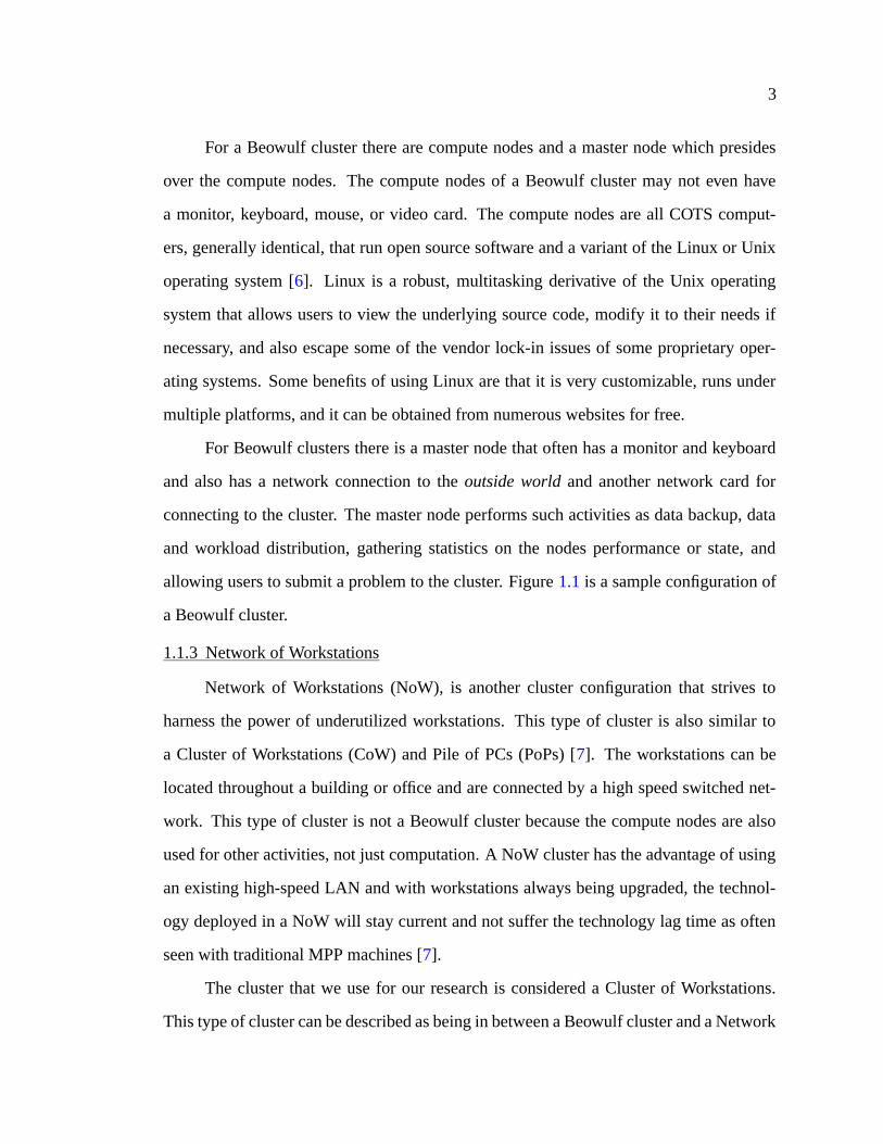
For a Beowulf cluster there are compute nodes and a master node which presides
over the compute nodes. The compute nodes of a Beowulf cluster may not even have
a monitor, keyboard, mouse, or video card. The compute nodes are all COTS comput-
ers, generally identical, that run open source software and a variant of the Linux or Unix
operating system [6]. Linux is a robust, multitasking derivative of the Unix operating
system that allows users to view the underlying source code, modify it to their needs if
necessary, and also escape some of the vendor lock-in issues of some proprietary oper-
ating systems. Some benefits of using Linux are that it is very customizable, runs under
multiple platforms, and it can be obtained from numerous websites for free.
For Beowulf clusters there is a master node that often has a monitor and keyboard
and also has a network connection to the outside world and another network card for
connecting to the cluster. The master node performs such activities as data backup, data
and workload distribution, gathering statistics on the nodes performance or state, and
allowing users to submit a problem to the cluster. Figure 1.1 is a sample configuration of
a Beowulf cluster.
1.1.3 Network of Workstations
Network of Workstations (NoW), is another cluster configuration that strives to
harness the power of underutilized workstations. This type of cluster is also similar to
a Cluster of Workstations (CoW) and Pile of PCs (PoPs) [7]. The workstations can be
located throughout a building or office and are connected by a high speed switched net-
work. This type of cluster is not a Beowulf cluster because the compute nodes are also
used for other activities, not just computation. A NoW cluster has the advantage of using
an existing high-speed LAN and with workstations always being upgraded, the technol-
ogy deployed in a NoW will stay current and not suffer the technology lag time as often
seen with traditional MPP machines [7].
The cluster that we use for our research is considered a Cluster of Workstations.
This type of cluster can be described as being in between a Beowulf cluster and a Network
4
Figure 1.1. Beowulf layout
of Workstations. Workstations are used for computation and other activities as with NoWs
but are also more isolated from the campus network as with a Beowulf cluster.

CHAPTER 2NETWORK SETUP
In this chapter different aspects of setting up a high performance computational
network will be discussed. The steps taken to install the software so that the computers
can communicate with each other, how the hardware is configured, how the network is
secured, and also how the internal computers can still access the World Wide Web will be
explained.
2.1 Network and Computer Hardware
The cluster that was built in our lab is considered a Cluster of Workstations, or
CoW. Other similar clusters are Network of Workstations (NoW), and Pile of PCs (PoPs).
The cluster consists of Commodity Off The Shelf (COTS) components, linked together
by switched Ethernet.
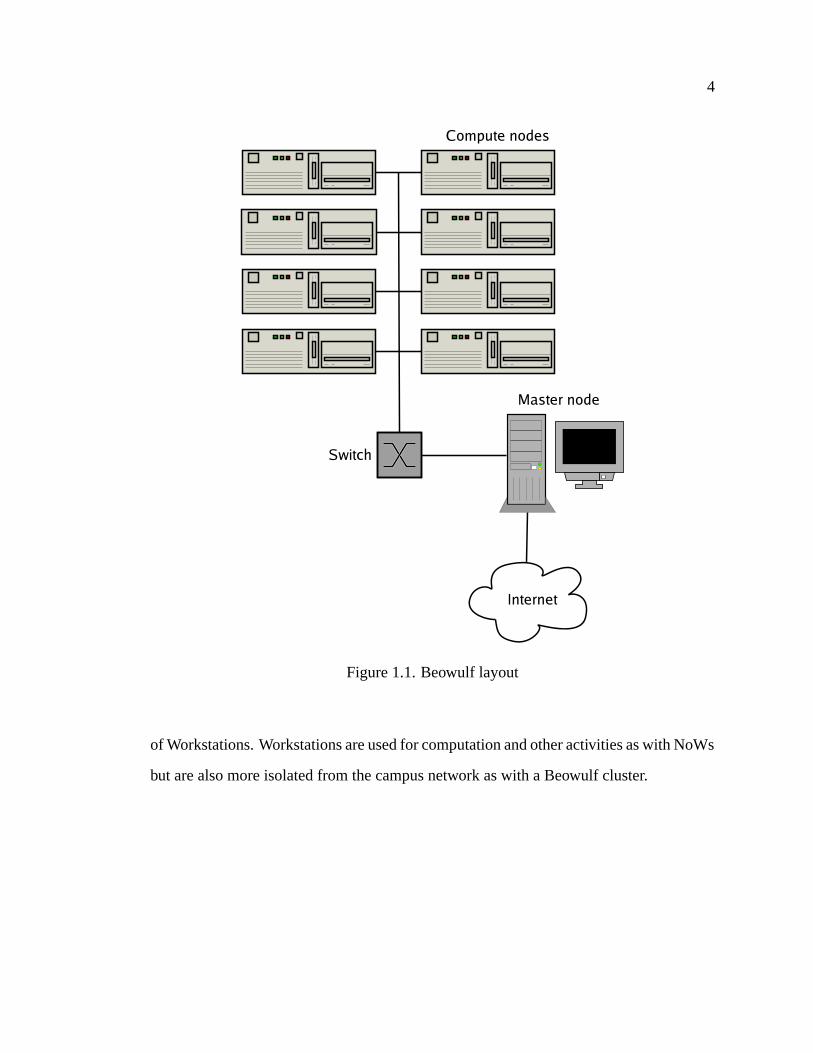
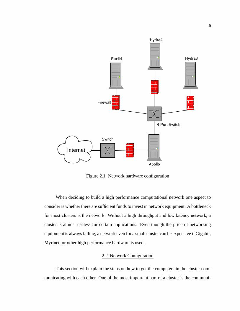
The cluster consists of four nodes, apollo, euclid, hydra3, and hydra4 with apollo
being the master node. They are arranged as shown in Figure 2.1.
Hydra3 and hydra4 each have one 2.0 GHz Pentium 4 processor with 512 KB L2
cache, Streaming SIMD Extensions 2 (SSE2), and operate on a 400 MHz system bus.
Both hydra3 and hydra4 have 40 GB Seagate Barracuda hard drives, operating at 7200
rpm, with 2 MB cache. Apollo and euclid each have one 2.4 GHz Pentium 4 processor
with 512 KB L2 cache, SSE2, and also operate on a 400 MHz system bus. Apollo and
euclid each have a 30 GB Seagate Barracuda drive operating at 7200 rpm and with a 2
MB cache. Each computer in the cluster has 1 GB of PC2100 DDRAM. The computers
are connected by a Netgear FS605 5 port 10/100 switch. As you can probably tell by the
above specs, our budget is a little on the low side.
5
6
Figure 2.1. Network hardware configuration
When deciding to build a high performance computational network one aspect to
consider is whether there are sufficient funds to invest in network equipment. A bottleneck
for most clusters is the network. Without a high throughput and low latency network, a
cluster is almost useless for certain applications. Even though the price of networking
equipment is always falling, a network even for a small cluster can be expensive if Gigabit,
Myrinet, or other high performance hardware is used.
2.2 Network Configuration
This section will explain the steps on how to get the computers in the cluster com-
municating with each other. One of the most important part of a cluster is the communi-
7
cation backbone on which data is transferred. By properly configuring the network, the
performance of a cluster is maximized and its construction is more justifiable. Each node
in the cluster is running Red Hat’s Fedora Core One [8] with a 2.4.22-1.2115.nptl kernel
[9].
2.2.1 Configuration Files
Internet Protocol (IP) is a data-oriented method used for communication over a
network by source and destination hosts. Each host on the end of an IP communication
has an IP address that uniquely identifies it from all other computers. IP sends data
between hosts split into packets and the Transmission Control Protocol (TCP) puts the
packets back together.
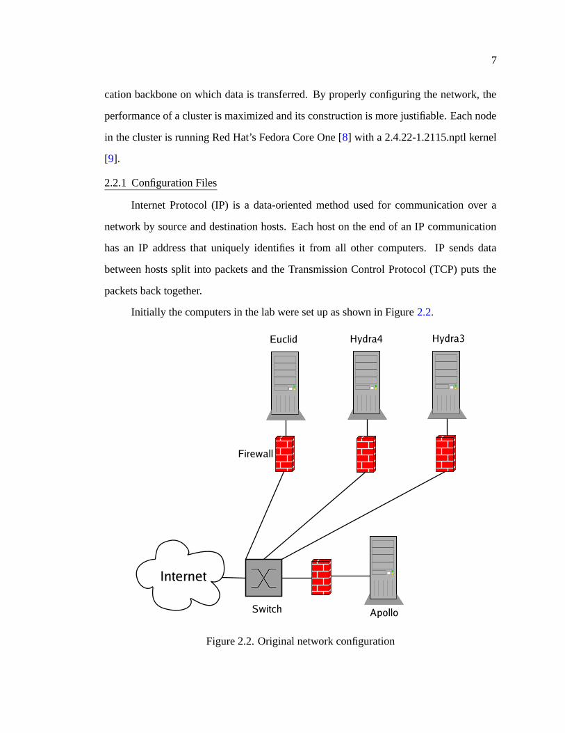
Initially the computers in the lab were set up as shown in Figure 2.2.
Figure 2.2. Original network configuration
8
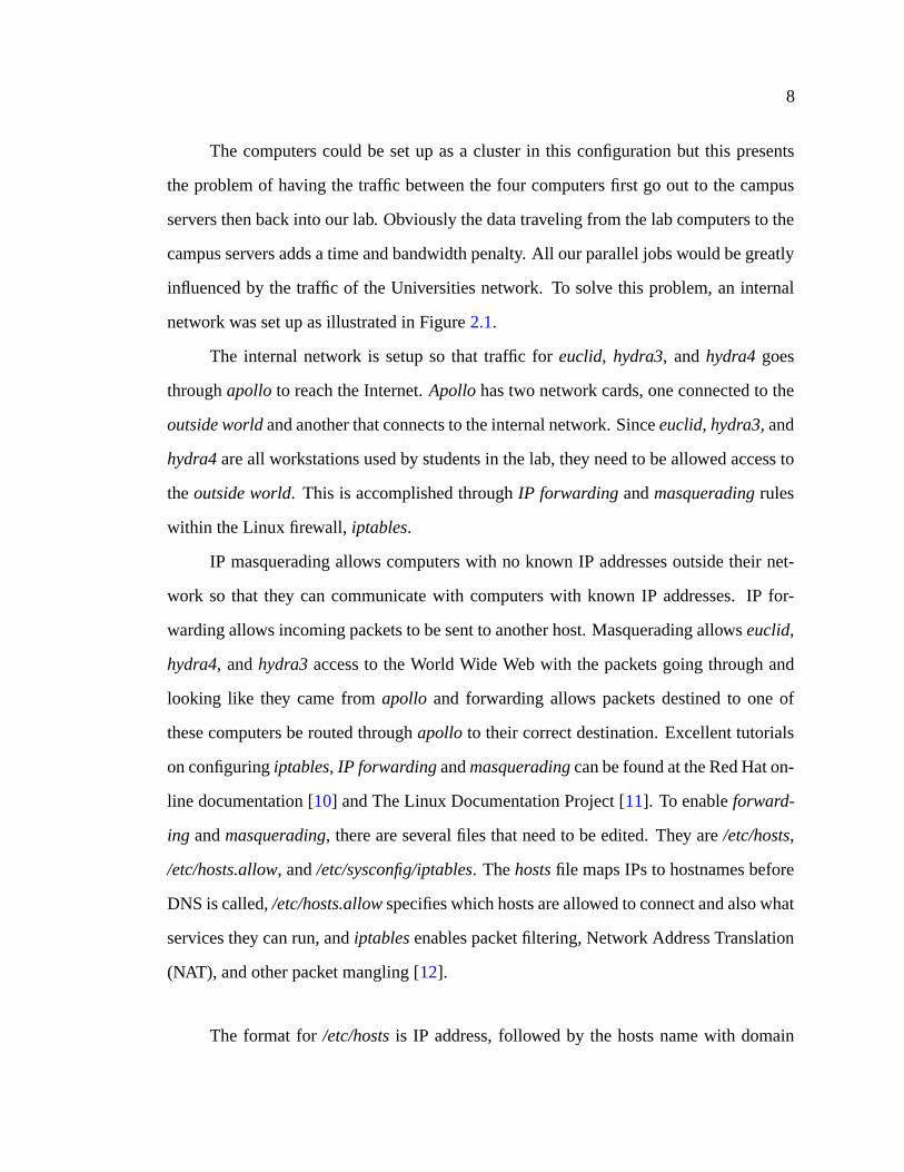
The computers could be set up as a cluster in this configuration but this presents
the problem of having the traffic between the four computers first go out to the campus
servers then back into our lab. Obviously the data traveling from the lab computers to the
campus servers adds a time and bandwidth penalty. All our parallel jobs would be greatly
influenced by the traffic of the Universities network. To solve this problem, an internal
network was set up as illustrated in Figure 2.1.
The internal network is setup so that traffic for euclid, hydra3, and hydra4 goes
through apollo to reach the Internet. Apollo has two network cards, one connected to the
outside world and another that connects to the internal network. Since euclid, hydra3, and
hydra4 are all workstations used by students in the lab, they need to be allowed access to
the outside world. This is accomplished through IP forwarding and masquerading rules
within the Linux firewall, iptables.
IP masquerading allows computers with no known IP addresses outside their net-
work so that they can communicate with computers with known IP addresses. IP for-
warding allows incoming packets to be sent to another host. Masquerading allows euclid,
hydra4, and hydra3 access to the World Wide Web with the packets going through and
looking like they came from apollo and forwarding allows packets destined to one of
these computers be routed through apollo to their correct destination. Excellent tutorials
on configuring iptables, IP forwarding and masquerading can be found at the Red Hat on-
line documentation [10] and The Linux Documentation Project [11]. To enable forward-
ing and masquerading, there are several files that need to be edited. They are /etc/hosts,
/etc/hosts.allow, and /etc/sysconfig/iptables. The hosts file maps IPs to hostnames before
DNS is called, /etc/hosts.allow specifies which hosts are allowed to connect and also what
services they can run, and iptables enables packet filtering, Network Address Translation
(NAT), and other packet mangling [12].
The format for /etc/hosts is IP address, followed by the hosts name with domain
9
information, and an alias for the host. For our cluster, each computer has all the other
computers in the cluster listed and also several computers on the University’s network.
For example, a partial hosts file for apollo is:
192.168.0.3 euclid.xxx.ufl.edu euclid
192.168.0.5 hydra4.xxx.ufl.edu hydra4
192.168.0.6 hydra3.xxx.ufl.edu hydra3
The file /etc/hosts.allow specifies which hosts are allowed to connect and what ser-
vices they are allowed to use, i.e. sshd and sendmail. This is the first checkpoint for all in-
coming network traffic. If a computer that is trying to connect is not listed in hosts.allow,
it will be rejected. The file has the format of the name of the daemon access will be
granted too followed by the host that is allowed access to that daemon, and then ALLOW.
For example, a partial hosts.allow file for apollo is:
ALL: 192.168.0.3: ALLOW
ALL: 192.168.0.5: ALLOW
ALL: 192.168.0.6: ALLOW
This will allow euclid, hydra4, and hydra3 access to all services on apollo.
2.2.2 Internet Protocol Forwarding and Masquerading
When information is sent over a network, it travels from its origin to its destination
in packets. The beginning of the packet, header, specifies its destination, where it came
from, and other administrative details [12]. Using this information, iptables can, using
specified rules, filter the traffic, dropping/accepting packets according to these rules, and
redirect traffic to other computers. Rules grouped into chains, and chains are grouped
into tables. By iptables, I am also referring to the underlying netfilter framework. The
netfilter framework is a set of hooks within the kernel that inspects packets while iptables
configures the netfilter rules.
10
Because all the workstations in the lab require access to the Internet, iptables will
be used to forward packets to specified hosts and also allow the computers to have a
private IP address that is masqueraded to look like it has a public IP address. The goal
of this section is not to explain in detail all the rules specified in our iptables file but to
just explain how forwarding and masquerading are set up. For our network we have an
iptables script, named iptables script, that sets the rules for iptables. The script is located
in /etc/sysconfig/. To run the script, simply type as root:
root@apollo> ./iptables_script
This will make active the rules defined in the script. To ensure that these rules
are loaded each time the system is rebooted, create the file iptables in the directory
/etc/sysconfig with the following command:
root@apollo> /sbin/iptables-save -c > iptables
To set up IP forwarding and masquerading, first open the file
/etc/sysconfig/networking/devices/ifcfg-eth1. There are two network cards in apollo, eth0,
which is connected to the external network, and eth1, which is connected to the internal
network. Add the following lines to ifcfg-eth1:
IPADDR=192.168.0.4
NETWORK=192.168.0.0
NETMASK=255.255.255.0
BROADCAST=192.168.0.255
This will set the IP address of eth1 to 192.168.0.4. Next, open the file
iptables script and add the following lines to the beginning of the file:
# Disable forwardingecho 0 > /proc/sys/net/ipv4/ip_forward
# load some modules (if needed)
11
# Flushiptables -t nat -F POSTROUTINGiptables -t nat -F PREROUTINGiptables -t nat -F OUTPUTiptables -F
# Set some parametersLAN_IP_NET=’192.168.0.1/24’LAN_NIC=’eth1’FORWARD_IP=’192.168.0.4’
# Set default policiesiptables -P INPUT DROPiptables -P FORWARD DROPiptables -P OUTPUT ACCEPT
# Enable masquerading and forwardingiptables -t nat -A POSTROUTING -s $LAN_IP_NET -j MASQUERADEiptables -A FORWARD -j ACCEPT -i $LAN_NIC -s $LAN_IP_NETiptables -A FORWARD -m state --state ESTABLISHED,RELATED -j ACCEPT
# Open SSH of apollo to LANiptables -A FORWARD -j ACCEPT -p tcp --dport 22iptables -t nat -A PREROUTING -i eth0 -p tcp --dport 22 -j DNAT \--to 192.168.0.4:22
# Enable forwardingecho 1 > /proc/sys/net/ipv4/ip_forward
Following the above lines is the original iptables script rules. First, IP forwarding
is disabled and the present running iptables rules are flushed. Next, some alias’ are set that
just make it easier to read and write the rules. After that, the default policies are set. All
incoming and forwarded traffic will be dropped and all packets sent out will be allowed.
With just these rules in place, there would be no incoming traffic allowed. Now, with the
default policies in place, other rules will be appended to them so that certain connections
are allowed. By setting INPUT and FORWARD to ACCEPT, the network would allow
unrestricted access, NOT a good idea! The next three lines enable masquerading of the
internal network via NAT (Network Address Translation) so that all traffic appears to be
coming from a single IP address, apollo’s, and forwarding of IP packets to the internal
network. Next, SSH is allowed between the computers on the internal network and apollo.
Finally, IP forwarding is enabled in the kernel.
12
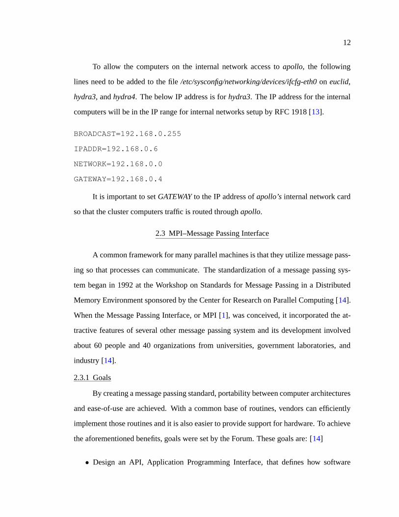
To allow the computers on the internal network access to apollo, the following
lines need to be added to the file /etc/sysconfig/networking/devices/ifcfg-eth0 on euclid,
hydra3, and hydra4. The below IP address is for hydra3. The IP address for the internal
computers will be in the IP range for internal networks setup by RFC 1918 [13].
BROADCAST=192.168.0.255
IPADDR=192.168.0.6
NETWORK=192.168.0.0
GATEWAY=192.168.0.4
It is important to set GATEWAY to the IP address of apollo’s internal network card
so that the cluster computers traffic is routed through apollo.
2.3 MPI–Message Passing Interface
A common framework for many parallel machines is that they utilize message pass-
ing so that processes can communicate. The standardization of a message passing sys-
tem began in 1992 at the Workshop on Standards for Message Passing in a Distributed
Memory Environment sponsored by the Center for Research on Parallel Computing [14].
When the Message Passing Interface, or MPI [1], was conceived, it incorporated the at-
tractive features of several other message passing system and its development involved
about 60 people and 40 organizations from universities, government laboratories, and
industry [14].
2.3.1 Goals
By creating a message passing standard, portability between computer architectures
and ease-of-use are achieved. With a common base of routines, vendors can efficiently
implement those routines and it is also easier to provide support for hardware. To achieve
the aforementioned benefits, goals were set by the Forum. These goals are: [14]
• Design an API, Application Programming Interface, that defines how software

13
communicates with one another.
• Allow efficient communication by avoiding memory-to-memory copying and al-
lowing overlap of computation and communication.
• Allow the software using MPI to be used in a heterogeneous environment.
• Allow convenient C and Fortran 77 bindings for the interface.
• Make the communication interface reliable
• Define an interface that is not too different from other libraries and provide exten-
sions for greater flexibility.
• Define an interface that can be run on many different hardware platforms such as
distributed memory multiprocessors and networks of workstations
• Semantics of the interface should be language independent.
• The interface should be designed to allow for thread safety.
The above goals offer great benefit for the programmer of all application sizes. By
keeping the logical structure of MPI language independent, new programmers to MPI
will more readily grasp the concepts while programmers of large applications will benefit
from the similarity to other libraries and also the C and F77 bindings.
There are some aspects that are not included in the standard. These include: [14]
• Explicit shared-memory operations.
• Program construction tools.
• Debugging facilities.
• Support for task management.
14
2.3.2 MPICH
There are many implementations of MPI; MPI/Pro, Chimp MPI, implementations
by hardware vendors IBM, HP, SUN, SGI, Digital, and others, with MPICH and LAM/MPI
being the two main ones. MPICH began in 1992 as an implementation that would track
the MPI standard as it evolved and point out any problems that developers may incur and
was developed at Argonne National Laboratory and Mississippi State University [15].
2.3.3 Installation
MPICH can be downloaded from the MPICH website at
http://www-unix.mcs.anl.gov/mpi/mpich/. The version that is run in our lab is 1.2.5.2.
The installation of MPICH is straightforward. Download the file mpich.tar.gz and uncom-
press. The directory in which MPICH is installed on our system is home/apollo/hda8.
redboots@apollo> gunzip mpich.tar.gz
redboots@apollo> tar -xvf mpich.tar
This creates the directory mpich-1.2.5.2.
The majority of the code for MPICH is device independent and is implemented on
top of an Abstract Device Interface or ADI. This allows MPICH to be more easily ported
to new hardware architectures by hiding most hardware specific details [16]. The ADI
used for networks of workstations is the ch p4 device, where ch stands for ”Chameleon”,
a symbol of adaptability and portability, and p4 stands for ”portable programs for parallel
processors” [15].
2.3.4 Enable SSH
The default process startup mechanism for the ch p4 device on networks is remote
shell or rsh. Rsh allows the execution of commands on remote hosts [17]. Rsh works
only if you are allowed to log into a remote machine without a password. Rsh relies on
the connection coming from a known IP address on a privileged port. This creates a huge
security risk because of the ease in which hackers can spoof the connection. A more
15
secure alternative to rsh is to use the Secure Shell or SSH protocol, which encrypts the
connection and uses digital signatures to positively identify the host at the other end of the
connection [17]. If we were to just create a computational network that was not connected
to the Internet, rsh would be fine. Since all our computers in the lab are connected to the
Internet, using insecure communication could possibly result in the compromise of our
system by hackers.
To set up SSH to work properly with MPICH, several steps need to be done. First
make sure SSH is installed on the computers on the network. Most standard installa-
tions of Linux come with SSH installed. If it is not, SSH can be downloaded from
http://www.openssh.com. Next, an authentication key needs to be created. Go to the
.ssh folder located in your home directory and type ssh-keygen -f identity -t rsa. When
the output asks you for a passphrase, just press Enter twice.
redboots@apollo> ssh-keygen -f identity -t rsa
Generating public/private rsa key pair.
Enter passphrase (empty for no passphrase):
Enter same passphrase again:
Your identification has been saved in identity.
Your public key has been saved in identity.pub.
The key fingerprint is:
43:68:68:30:79:73:e2:03:d9:50:2b:f1:c1:5d:e7:60
This will create two files identity and identity.pub. Now place the identity.pub key
in the file $HOME/.ssh/authorized keys where $HOME is the users home directory. If the
users home directory is not a shared file system, authorized keys should be copied into
$HOME/.ssh/authorized keys on each computer.
16
Also, if the file authorized keys does not exist, create it.
redboots@apollo> touch authorized_keys
Finally, while in $HOME/.ssh, type:
redboots@apollo> ssh-agent $SHELL
redboots@apollo> ssh-add
The above commands will allow the user to avoid typing in the pass phrase each
time SSH is invoked [18].
Now enter into the main MPICH directory and type:
redboots@apollo> ./configure -rsh=ssh
This will configure MPICH to use SSH instead of rsh. The above steps of installing
MPICH need to be performed for all the computers that are to be in the cluster.
2.3.5 Edit Machines.LINUX
In order for the master node to know which computers are available for the cluster,
the file machines.LINUX needs to be edited. After MPICH is installed on all the comput-
ers, open the file
/home/apollo/hda8/mpich-1.2.5.2/util/machines/machines.LINUX on the master node, apollo
in our case, and edit it so that each node of the cluster is listed. In order to run an MPI
program, the number of processors to use needs to be specified:
redboots@apollo> mpirun -np 4 program
In the above example, 4 is the number of processors that are used to run program.
When the execution begins, mpirun reads the file machines.LINUX to see what machines
are available in the cluster. If the number of processors specified by the -np flag are more
than what is listed in machines.LINUX, the difference will be made up by some processors
doing more work. To achieve the best performance, it is recommended that the number
17
of processors listed in machines.LINUX is equal to or more than -np. The format for
machines.LINUX is very straightforward, hostname:number of CPUs. For each line, a
hostname is listed and, if a machine has more than one processor, a colon followed by
the number of processors. For example, if there were two machines in the cluster with
machine1 having one processor and machine2 having four processors, machines.LINUX
would be as follows:
machine1
machine2:4
The machines.LINUX file that apollo uses is:
apollo.xxx.ufl.edu
euclid.xxx.ufl.edu
hydra4.xxx.ufl.edu
hydra3.xxx.ufl.edu
Because all our compute nodes have single processors, a colon followed by a num-
ber is not necessary.
2.3.6 Test Examples
MPICH provides several examples to test whether the network and software
are setup correctly. One example computes Pi and is located in /home/apollo/hda8/mpich-
1.2.5.2/examples/basic. The file cpi.c contains the source code. To calculate Pi, cpi solves
the Gregory-Leibniz series over a user specified number of intervals, n. MPI programs
can be really small, using just six functions or they can be very large, using over one hun-
dred functions. The four necessary functions that cpi uses are MPI Init, MPI Finalize,
MPI Comm size, MPI Comm rank, with MPI Bcast and MPI Reduce used to send and
reduce the returned data to a single number, respectively. The code for cpi.c is seen in
18
Appendix A. After the desired number of intervals n is defined in cpi.c, simply com-
pile cpi by typing at a command prompt:
redboots@apollo> make cpi
/home/apollo/hda8/mpich-1.2.5.2/bin/mpicc -c cpi.c
/home/apollo/hda8/mpich-1.2.5.2/bin/mpicc -o cpi cpi.o \
-lm
This will create the executable cpi. To run cpi, while at a command prompt in
/home/apollo/hda8/mpich-1.2.5.2/examples/basic, enter the following:
redboots@apollo> mpirun -np 4 cpiProcess 0 of 4 on apollo.xxx.ufl.edupi is approximately 3.1415926535899033, Error is 0.00000000000011wall clock time = 0.021473Process 3 of 4 on hydra3.xxx.ufl.eduProcess 2 of 4 on hydra4.xxx.ufl.eduProcess 1 of 4 on euclid.xxx.ufl.edu
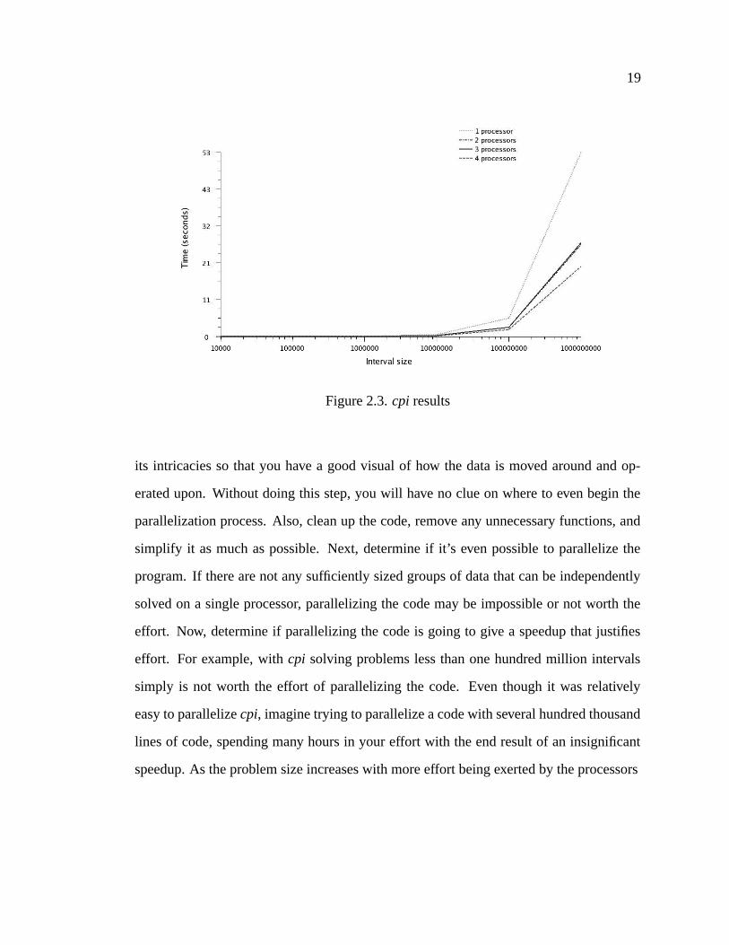
Several tests were run while varying the number of intervals and processors. These
results are summarized in Figure 2.3.
2.3.7 Conclusions
Depending on the complexity of your application, MPI can be relatively simple to
integrate. If the problem is easy to split and divide the work evenly among the processors,
like the example that computes Pi, as little as six functions may be used. For all problems,
the user needs to decide how to partition the work, how to send it to the other processors,
decide if the processors have to communicate with one another, and decide what to do
with the solution that each node computes, which all can be done with a few functions if
the problem is not too complicated.
When deciding whether to parallelize a program, several things should be consid-
ered and performed. First, really understand how the serial code works. Study it and all
19
Figure 2.3. cpi results
its intricacies so that you have a good visual of how the data is moved around and op-
erated upon. Without doing this step, you will have no clue on where to even begin the
parallelization process. Also, clean up the code, remove any unnecessary functions, and
simplify it as much as possible. Next, determine if it’s even possible to parallelize the
program. If there are not any sufficiently sized groups of data that can be independently
solved on a single processor, parallelizing the code may be impossible or not worth the
effort. Now, determine if parallelizing the code is going to give a speedup that justifies
effort. For example, with cpi solving problems less than one hundred million intervals
simply is not worth the effort of parallelizing the code. Even though it was relatively
easy to parallelize cpi, imagine trying to parallelize a code with several hundred thousand
lines of code, spending many hours in your effort with the end result of an insignificant
speedup. As the problem size increases with more effort being exerted by the processors

20
than the network, parallelization becomes more practical. With small problems, less than
one-hundred million intervals for the cpi example, illustrated by the results in Figure 2.3,
the penalty of latency in a network simply does not justify parallelization.
CHAPTER 3BENCHMARKING
In this chapter cluster benchmarking will be discussed. There are several reasons
why benchmarking a cluster is important. One being determining the sensitivity of the
cluster to network parameters. Such parameters include bandwidth and latency. Another
reason to benchmark is to determine how scalable your cluster is. Will performance scale
with the addition of more compute nodes enough such that the price/performance ratio
is acceptable? Testing scalability will help determine the best hardware and software
configuration such that the practicality of using some or all of the compute nodes is de-
termined.
3.1 Performance Metrics
An early measure of performance that was used to benchmark machines was MIPS
or Million Instructions Per Second. This benchmark refers to the number of low-level
machine code instructions that a processor can execute in one second. This benchmark,
however, does not take into effect that all chips are not the same in the way that they
handle instructions. For example, a 2.0 GHz 32bit processor will have a 2000 MIPS
rating and a 2.0 GHz 64 bit processor will also have a 2000 MIPS rating. This is an
obviously flawed rating because software written specifically for the 64 bit processor will
solve a comparable problem much faster than a 32 bit processor with software written
specifically for it.
The widely accepted metric of processing power used today is FLOPS or Floating
Point Operations Per Second. This benchmark unit measures the number of calculations
that a computer can perform on a floating point number, or a number with a certain preci-
sion. A problem with this measurement is that it does not take into account the conditions
21
22
in which the benchmark is being conducted. For example, if a machine is being bench-
marked and also being subjected to an intense computation simultaneously, the reported
FLOPS will be lower. However, for its shortcomings, the FLOPS is widely used to mea-
sure cluster performance. The actual answer to all benchmark questions is found when
the applications for the cluster are installed and tested. When the actual applications and
not just a benchmark suite are tested, a much more accurate assessment of the clusters
performance is obtained.
3.2 Network Analysis
In this section, NetPIPE(Network Protocol Independent Performance Evaluator)
will be discussed [19]. The fist step to benchmarking a cluster is to determine if the
network you are using is operating efficiently and to get an estimate on its performance.
From the NetPIPE website, ”NetPIPE is a protocol independent tool that visually repre-
sents network performance under a variety of conditions” [19]. NetPIPE was originally
developed at the Scalable Computing Laboratory by Quinn Snell, Armin Mikler, John
Gustafson, and Guy Helmer. It is currently being developed and maintained by Dave
Turner.
A major bottleneck in high performance parallel computing is the network on which
it communicates [20]. By identifying which factors affect interprocessor communication
the most and reducing their effect, application performance can be greatly improved. The
two major factors that affect overall application performance on a cluster are network la-
tency, the delay of when a piece of data is sent and when it is received, and the maximum
sustainable bandwidth, the amount of data that can be sent over the network continuously
[20]. Some other factors that affect application performance are CPU speed, the CPU
bus, cache size of CPU, and the I/O performance of the nodes hard drive.
23
Fine tuning the performance of a network can be a very time consuming and ex-
pensive process and requires a lot of knowledge on network hardware to fully utilize the
hardware’s potential. For this section I will not go into too many details about network
hardware. The minimum network hardware that should be used for a Beowulf today is
one based on one-hundred Megabit per second (100 Mbps) Ethernet technology. With
the increase in popularity and decrease costs of one-thousand Megabit per second (1000
Mbps) hardware, a much better choice would be Gigabit Ethernet. If very low latency,
high and sustainable bandwidth is required for your application, and cost isn’t too im-
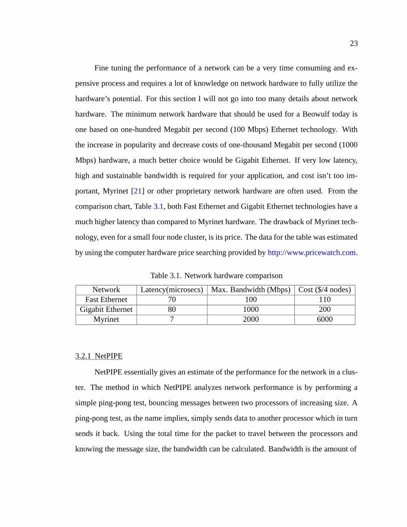
portant, Myrinet [21] or other proprietary network hardware are often used. From the
comparison chart, Table 3.1, both Fast Ethernet and Gigabit Ethernet technologies have a
much higher latency than compared to Myrinet hardware. The drawback of Myrinet tech-
nology, even for a small four node cluster, is its price. The data for the table was estimated
by using the computer hardware price searching provided by http://www.pricewatch.com.
Table 3.1. Network hardware comparison
Network Latency(microsecs) Max. Bandwidth (Mbps) Cost ($/4 nodes)Fast Ethernet 70 100 110
Gigabit Ethernet 80 1000 200Myrinet 7 2000 6000
3.2.1 NetPIPE
NetPIPE essentially gives an estimate of the performance for the network in a clus-
ter. The method in which NetPIPE analyzes network performance is by performing a
simple ping-pong test, bouncing messages between two processors of increasing size. A
ping-pong test, as the name implies, simply sends data to another processor which in turn
sends it back. Using the total time for the packet to travel between the processors and
knowing the message size, the bandwidth can be calculated. Bandwidth is the amount of
24
data that can be transferred through a network in a given amount of time. Typical units of
bandwidth are Megabits per second (Mbps) and Gigabits per second (Gbps).
To provide a complete and accurate test, NetPIPE uses message sizes at regular
intervals and at each data point, many ping-pong tests are carried out. This test will give
an overview of the unloaded CPU network performance. Applications may not reach the
reported maximum bandwidth because NetPIPE only measures the network performance
of unloaded CPUs, measuring the network performance with loaded CPUs is not yet
possible.
3.2.2 Test Setup
NetPIPE can be obtained from its website at
http://www.scl.ameslab.gov/netpipe/. Download the latest version and unpack. The in-
stall directory for NetPIPE on our system is home/apollo/hda8.
redboots@apollo> tar -xvzf NetPIPE_3.6.2.tar.gz
To install, enter the directory NetPIPE 3.6.2 that was created after unpacking the
above file. Edit the file makefile with your favorite text editor so that it points to the
correct compiler, libraries, include files, and directories. The file makefile did not need
any changes for our setup. To make the MPI interface, make sure the compiler is set to
mpicc. Next, in the directory NetPIPE 3.6.2, type make mpi:
redboots@apollo> make mpi
mpicc -O -DMPI ./src/netpipe.c ./src/mpi.c -o NPmpi -I./src
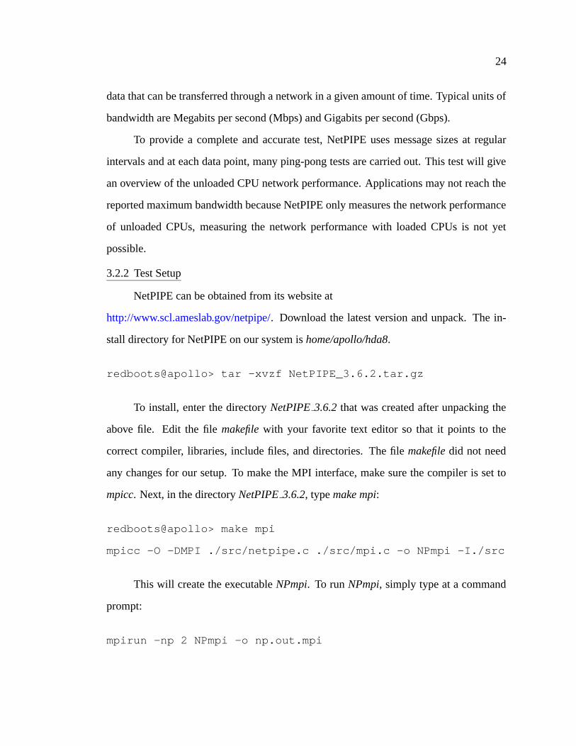
This will create the executable NPmpi. To run NPmpi, simply type at a command
prompt:
mpirun -np 2 NPmpi -o np.out.mpi
25
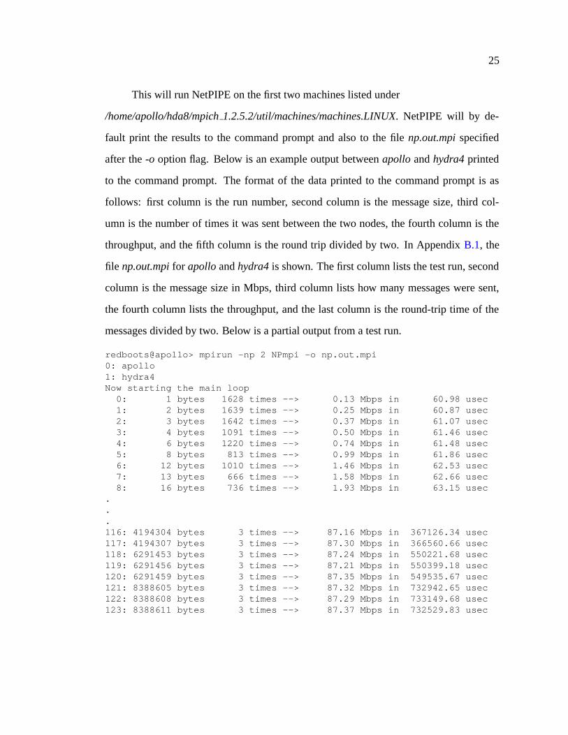
This will run NetPIPE on the first two machines listed under
/home/apollo/hda8/mpich 1.2.5.2/util/machines/machines.LINUX. NetPIPE will by de-
fault print the results to the command prompt and also to the file np.out.mpi specified
after the -o option flag. Below is an example output between apollo and hydra4 printed
to the command prompt. The format of the data printed to the command prompt is as
follows: first column is the run number, second column is the message size, third col-
umn is the number of times it was sent between the two nodes, the fourth column is the
throughput, and the fifth column is the round trip divided by two. In Appendix B.1, the
file np.out.mpi for apollo and hydra4 is shown. The first column lists the test run, second
column is the message size in Mbps, third column lists how many messages were sent,
the fourth column lists the throughput, and the last column is the round-trip time of the
messages divided by two. Below is a partial output from a test run.
redboots@apollo> mpirun -np 2 NPmpi -o np.out.mpi0: apollo1: hydra4Now starting the main loop0: 1 bytes 1628 times --> 0.13 Mbps in 60.98 usec1: 2 bytes 1639 times --> 0.25 Mbps in 60.87 usec2: 3 bytes 1642 times --> 0.37 Mbps in 61.07 usec3: 4 bytes 1091 times --> 0.50 Mbps in 61.46 usec4: 6 bytes 1220 times --> 0.74 Mbps in 61.48 usec5: 8 bytes 813 times --> 0.99 Mbps in 61.86 usec6: 12 bytes 1010 times --> 1.46 Mbps in 62.53 usec7: 13 bytes 666 times --> 1.58 Mbps in 62.66 usec8: 16 bytes 736 times --> 1.93 Mbps in 63.15 usec
.
.
.116: 4194304 bytes 3 times --> 87.16 Mbps in 367126.34 usec117: 4194307 bytes 3 times --> 87.30 Mbps in 366560.66 usec118: 6291453 bytes 3 times --> 87.24 Mbps in 550221.68 usec119: 6291456 bytes 3 times --> 87.21 Mbps in 550399.18 usec120: 6291459 bytes 3 times --> 87.35 Mbps in 549535.67 usec121: 8388605 bytes 3 times --> 87.32 Mbps in 732942.65 usec122: 8388608 bytes 3 times --> 87.29 Mbps in 733149.68 usec123: 8388611 bytes 3 times --> 87.37 Mbps in 732529.83 usec
26
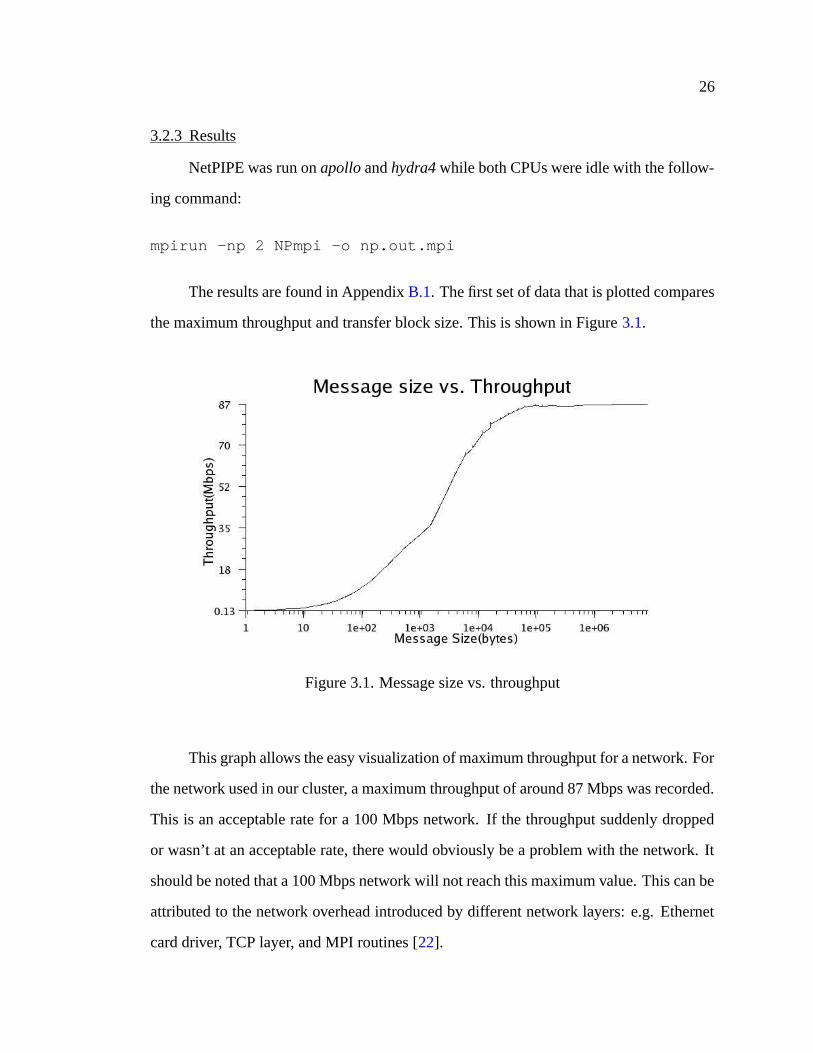
3.2.3 Results
NetPIPE was run on apollo and hydra4 while both CPUs were idle with the follow-
ing command:
mpirun -np 2 NPmpi -o np.out.mpi
The results are found in Appendix B.1. The first set of data that is plotted compares
the maximum throughput and transfer block size. This is shown in Figure 3.1.
Figure 3.1. Message size vs. throughput
This graph allows the easy visualization of maximum throughput for a network. For
the network used in our cluster, a maximum throughput of around 87 Mbps was recorded.
This is an acceptable rate for a 100 Mbps network. If the throughput suddenly dropped
or wasn’t at an acceptable rate, there would obviously be a problem with the network. It
should be noted that a 100 Mbps network will not reach this maximum value. This can be
attributed to the network overhead introduced by different network layers: e.g. Ethernet
card driver, TCP layer, and MPI routines [22].
27
NetPIPE also allows for the testing of TCP bandwidth without MPI induced over-
head. To run this test, first create the NPtcp executable. To install NPtcp on our cluster
required no changes to the file makefile in the NetPIPE 3.6.2 directory. To create the
NPtcp executable, simply type at the command prompt while in the NetPIPE 3.6.2 direc-
tory:
redboots@apollo> make tcp
cc -O ./src/netpipe.c ./src/tcp.c -DTCP -o NPtcp -I./src
This will create the executable NPtcp. To run the TCP benchmark, it requires both
a sender and receiver node. For example, in our TCP benchmarking test, hydra4 was
designated the receiver node and apollo the sender. This test obviously requires you to
open a terminal and install NPtcp on both machines unlike NPmpi which doesn’t require
you to open a terminal on the other tested machine, in this case hydra4.
First, log into hydra4. Install NPtcp on hydra4 following the above example. For
hydra4, the executable NPtcp is located in /home/hydra4/hda13/NetPIPE 3.6.2. While in
this directory, at a command prompt type ./NPtcp
redboots@hydra4> ./NPtcp
Send and receive buffers are 16384 and 87380 bytes
(A bug in Linux doubles the requested buffer sizes)
The above line will now allow hydra4 to be the receiver. For each separate run,
the above command needs to be retyped. Next, log into apollo and enter the directory in
which NPtcp is installed. For apollo, this is located in /home/apollo/hda8/NetPIPE 3.6.2.
While in this directory, at a command prompt start NPtcp while specifying hydra4 as the
receiver.
redboots@apollo> ./NPtcp -h hydra4 -o np.out.tcpSend and receive buffers are 16384 and 87380 bytes(A bug in Linux doubles the requested buffer sizes)
28
Now starting the main loop0: 1 bytes 2454 times --> 0.19 Mbps in 40.45 usec1: 2 bytes 2472 times --> 0.38 Mbps in 40.02 usec2: 3 bytes 2499 times --> 0.57 Mbps in 40.50 usec3: 4 bytes 1645 times --> 0.75 Mbps in 40.51 usec4: 6 bytes 1851 times --> 1.12 Mbps in 41.03 usec5: 8 bytes 1218 times --> 1.47 Mbps in 41.64 usec6: 12 bytes 1500 times --> 2.18 Mbps in 42.05 usec7: 13 bytes 990 times --> 2.33 Mbps in 42.54 usec
.
.
.116: 4194304 bytes 3 times --> 89.74 Mbps in 356588.32 usec117: 4194307 bytes 3 times --> 89.74 Mbps in 356588.50 usec118: 6291453 bytes 3 times --> 89.75 Mbps in 534800.34 usec119: 6291456 bytes 3 times --> 89.75 Mbps in 534797.50 usec120: 6291459 bytes 3 times --> 89.75 Mbps in 534798.65 usec121: 8388605 bytes 3 times --> 89.76 Mbps in 712997.33 usec122: 8388608 bytes 3 times --> 89.76 Mbps in 713000.15 usec123: 8388611 bytes 3 times --> 89.76 Mbps in 713000.17 usec
Running NPtcp will create the file np.out.tcp. The -h hydra4 option specifies the
hostname for the receiver, in this case hydra4. You can use either the IP-address or
the hostname if you have the receivers hostname and corresponding IP-address listed in
/etc/hosts. The -o np.out.tcp option specifies the output file to be named np.out.tcp. The
format of this file is the same as the np.out.mpi file created by NPmpi. The file np.out.tcp
is found in Appendix B.2.
To compare the overhead costs of MPI on maximum throughput, the throughput of
both the TCP and MPI runs were plotted compared to message size. In Figure 3.2 the
comparison of maximum throughput can be seen.
From Figure 3.2, the TCP overhead test consistently recorded a higher throughput
throughout the message size range as expected. Another interesting plot is to consider
message size versus the time the packets travel. This is seen in Figure 3.3
This plot shows the saturation point between sending data through TCP and with
MPI routines atop of TCP. The saturation point is the position on the graph after which an
increase in block size results in an almost linear increase in transfer time [23]. This point
is more easily located as being at the ”knee” of the curve. For both the TCP and MPI run,
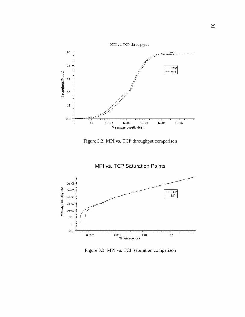
29
Figure 3.2. MPI vs. TCP throughput comparison
Figure 3.3. MPI vs. TCP saturation comparison
30
the saturation point occurred around 130 bytes. After that, both rose linearly together
with no distinction between the two after a message size of one Kilobyte. It can be con-
cluded overhead induced by MPI routines does not affect latency performance greatly for
message sizes above one-hundred thirty bytes.
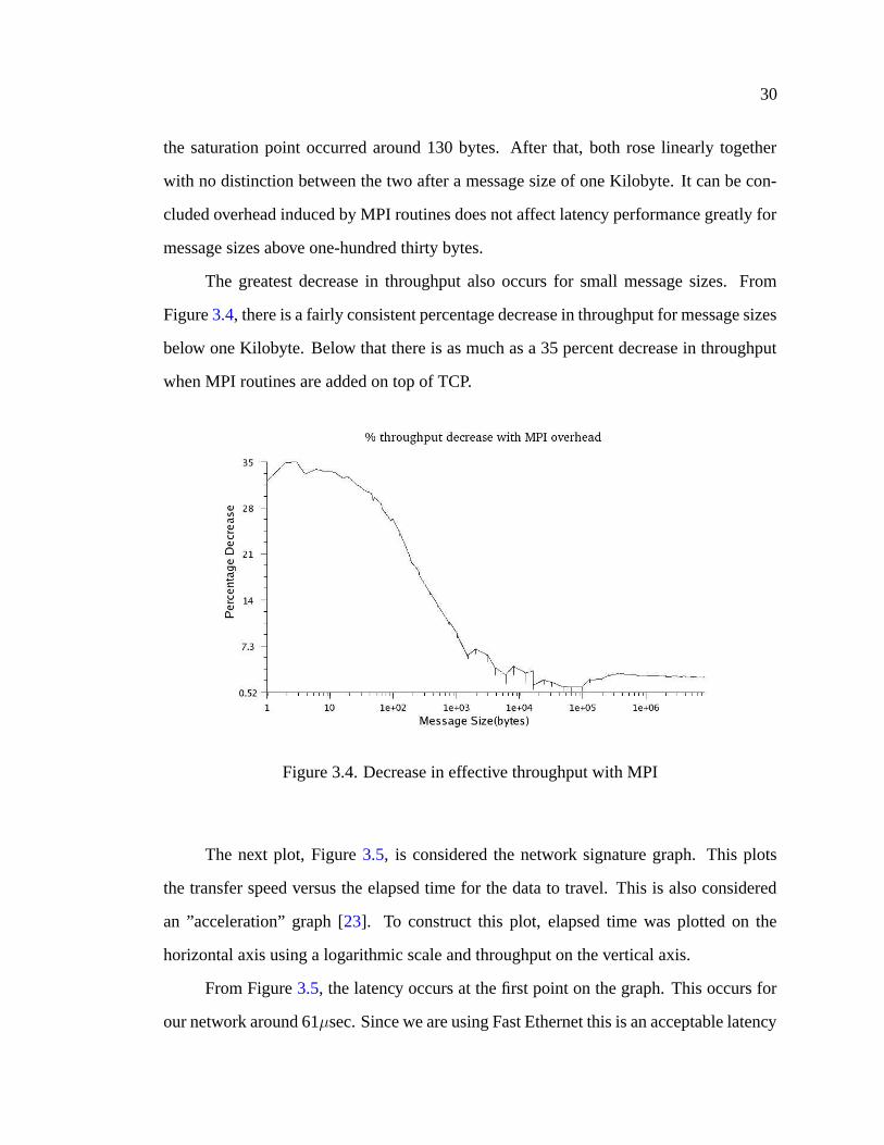
The greatest decrease in throughput also occurs for small message sizes. From
Figure 3.4, there is a fairly consistent percentage decrease in throughput for message sizes
below one Kilobyte. Below that there is as much as a 35 percent decrease in throughput
when MPI routines are added on top of TCP.
Figure 3.4. Decrease in effective throughput with MPI
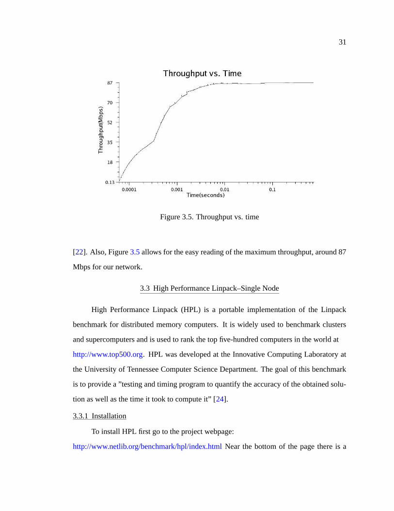
The next plot, Figure 3.5, is considered the network signature graph. This plots
the transfer speed versus the elapsed time for the data to travel. This is also considered
an ”acceleration” graph [23]. To construct this plot, elapsed time was plotted on the
horizontal axis using a logarithmic scale and throughput on the vertical axis.
From Figure 3.5, the latency occurs at the first point on the graph. This occurs for
our network around 61µsec. Since we are using Fast Ethernet this is an acceptable latency
31
Figure 3.5. Throughput vs. time
[22]. Also, Figure 3.5 allows for the easy reading of the maximum throughput, around 87
Mbps for our network.
3.3 High Performance Linpack–Single Node
High Performance Linpack (HPL) is a portable implementation of the Linpack
benchmark for distributed memory computers. It is widely used to benchmark clusters
and supercomputers and is used to rank the top five-hundred computers in the world at
http://www.top500.org. HPL was developed at the Innovative Computing Laboratory at
the University of Tennessee Computer Science Department. The goal of this benchmark
is to provide a ”testing and timing program to quantify the accuracy of the obtained solu-
tion as well as the time it took to compute it” [24].
3.3.1 Installation
To install HPL first go to the project webpage:
http://www.netlib.org/benchmark/hpl/index.html Near the bottom of the page there is a
32
hyperlink for hpl.tgz. Download the package to the directory of your choice. Unpack
hpl.tgz with the command:
tar -xvzf hpl.tgz
This will create the folder hpl.
Next, enter the directory hpl and copy the file Make.Linux PII CBLAS from the
setup directory to the main hpl directory and rename to Make.Linux P4:
redboots@apollo> cp setup/Make.Linux_PII_CBLAS \
Make.Linux_P4
There are several other Makefiles located in the setup folder for different architec-
tures. We are using Pentium 4’s so the Make.Linux PII CBLAS Makefile was chosen and
edited it so that it points to the correct libraries on our system. The Makefile that was used
for the compilation is shown in Appendix B.3.1. First, open the file in your favorite text
editor and edit it so that it points to your MPI directory and MPI libraries. Also, edit the
file so that it points to your correct BLAS (Basic Linear Algebra Subprograms) library as
described below. BLAS are routines for performing basic vector and matrix operations.
The website for BLAS is found at http://www.netlib.org/blas/. The Makefile which was
used for our benchmarking is located in Appendix B.3.1. Note the libraries which were
used for the benchmarks were either those provided by ATLAS or Kazushige Goto, which
will be discussed shortly.
After the Makefile is configured for your particular setup, HPL can now be com-
piled. To do this simply type at the command prompt:
make arch=Linux_P4
The HPL binary, xhpl , will be located in $hpl/bin/Linux P4. Also created is the file
HPL.dat which provides a way of editing parameters that affect the benchmarking results.
33
3.3.2 ATLAS Routines
For HPL, the most critical part of the software is the matrix-matrix multiplication
routine, DGEMM, that is a part of the BLAS. An optimized set of BLAS routines widely
used is ATLAS, or Automatically Tuned Linear Algebra Software [25]. The website
for ATLAS is located at http://math-atlas.sourceforge.net. The ATLAS routines strive to
create optimized software for different processor architectures.
To install precompiled ATLAS routines for a particular processor, first go to
http://www.netlib.org/atlas/archives. On this page are links for AIX, SunOS, Windows,
OS-X, IRIX, HP-IX, and Linux. Our cluster is using the Linux operating system so the
linux link was clicked. The next page lists precompiled routines for several processors,
including Pentium 4 with Streaming SIMD Extensions 2 (SSE2), the AMD Hammer
processor, PowerPC, Athlon, Itanium, and Pentium III. The processors that we are using
in the cluster are Pentium 4’s so the file atlas.6.0 Linux 4SSE2.tgz was downloaded. The
file was downloaded to /home/apollo/hda8 and unpacked.
redboots@apollo> tar -xvzf atlas3.6.0_Linux_P4SSE2.tgz
This creates the folder Linux P4SSE2. Within this directory is the Makefile that
was used to compile the libraries, the folder containing the precompiled libraries, lib, and
in the include directory, the C header files for the C interface to BLAS and LAPACK. To
link to the precompiled ATLAS routines in HPL, simply point to the routines
LAdir = /home/apollo/hda8/Linux_P4SSE2/lib
LAlib = $(LAdir)/libcblas.a $(LAdir)/libatlas.a
Also, for the ATLAS libraries, uncomment the line that reads:
HPL_OPTS = -DHPL_CALL_CBLAS
Finally, compile the executable xhpl as shown above. Enter the main HPL directory
and type make arch=Linux P4
34
redboots@apollo> make arch=Linux_P4
This creates the executable xhpl and the configuration file HPL.dat
3.3.3 Goto BLAS Libraries
Initially, the ATLAS routines were used in HPL to benchmark the cluster. The re-
sults of the benchmark using the ATLAS routines were then compared to the results using
another optimized set of BLAS routines developed by Kazushige Goto [26]. The libraries
developed by Kazushige Goto are located at
http://www.cs.utexas.edu/users/kgoto/signup first.html. The libraries located at this web-
site are optimized BLAS routines for a number of processors including Pentium III, Pen-
tium IV, AMD Opteron, Itanium2, Alpha, and PPC. A more in depth explanation as to
why this library performs better than ATLAS is located at
http://www.cs.utexas.edu/users/flame/goto/. To use these libraries on our cluster, the
routines optimized for Pentium 4’s with 512 Kb L2 cache were used, libgoto p4 512-
r0.96.so.gz. Also the file xerbla.f needs to be downloaded which is located at
http://www.cs.utexas.edu/users/kgoto/libraries/xerbla.f. This file is simply an error han-
dler for the routines.
To use these routines, first download the appropriate file for your architecture and
download xerbla.f. For our cluster, libgoto p4 512-r0.96.so.gz was downloaded to
/home/apollo/hda8/goto blas. Unpack the file libgoto p4 512-r0.96.so.gz.
redboots@apollo> gunzip libgoto_p4_512-r0.96.so.gz
This creates the file libgoto p4 512-r0.96.so. Next, download the file xerbla.f from
the website listed above to /home/apollo/hda8/goto blas. Next, create the binary object
file for xerbla.f
redboots@apollo> g77 -c xerbla.f
35
This will create the file xerbla.o. These two files, libgoto p4 512-r0.96.so and
xerbla.o need to be pointed to in the HPL Makefile.
LAdir = /home/apollo/hda8/goto_blas
LAlib = $(LAdir)/libgoto_p4_512-r0.96.so $(LAdir)/xerbla.o
Also the following line needs to be commented. By placing a pound symbol in front
of a line tells the compiler to ignore that line and treat it as text.
#HPL_OPTS = -DHPL_CALL_CBLAS
3.3.4 Using either Library
Two sets of tests were carried out with HPL: one using the ATLAS routine and the
other using Kazushige Goto’s routine. These tests were carried for several reasons. One
is to illustrate the importance of using well written and compiled software on a clusters
performance. Without well written software that is optimized for a particular hardware
architecture or network topography, performance of a cluster suffers greatly. Another
reason why two tests using the different BLAS routines were conducted is to get a more
accurate assessment on our clusters performance. By using a benchmark, we have an
estimate on how our applications should perform. If the parallel applications that we use
perform at a much lower level than the benchmark, then that would allow us to conclude
that our software isn’t tuned for our particular hardware properly or the software contains
inefficient coding.
Below, the process of using either ATLAS or Kazushige Goto’s BLAS routines will
be discussed. The first tests that were conducted used the ATLAS routines. Compile the
HPL executable, xhpl, as described above for the ATLAS routines using the file Makefile
in Appendix B.3.1. After the tests are completed using the ATLAS routines simply change
the links to Goto’s BLAS routines and comment the line that calls the BLAS Fortran 77
interface. For example, the section of the Makefile which we use that determines which
36
library to use is seen below. For the below section of the Makefile, Goto’s BLAS routines
are specified.
# Below the user has a choice of using either the ATLAS or Goto# BLAS routines. To use the ATLAS routines, uncomment the# following 2 lines and comment the 3rd and 4th. To use Goto’s BLAS# routines, comment the first 2 lines and uncomment line 3rd and# 4th.
# BEGIN BLAS specificationLAdir = /home/apollo/hda8/hpl/librariesLAlib = $(LAdir)/libgoto_p4_512-r0.96.so $(LAdir)/xerbla.o#LAdir = /home/apollo/hda8/Linux_P4SSE2/lib#LAlib = $(LAdir)/libcblas.a $(LAdir)/libatlas.a# END BLAS specification
If Goto’s routines are to be used, just uncomment the two lines that specify those
routines and comment the two lines for the ATLAS routines. The line that specifies the
BLAS Fortran 77 interface is also commented when using Goto’s BLAS routines.
#HPL_OPTS = -DHPL_CALL_CBLAS
If the ATLAS routines are to be used, the above line would be uncommented. After
that xhpl is recompiled using the method described above.
redboots@apollo> make arch=Linux_P4
3.3.5 Benchmarking
To determine a FLOPS value for the machine(s) to be benchmarked, HPL solves
a random dense linear system of equations in double precision. HPL solves the random
dense system by first computing the LU factorization with row-partial pivoting and then
solving the upper triangular system. HPL is very scalable, it is the benchmark used on
the supercomputers with thousands of processors found at
Top 500 List of Supercomputing Sites and can be used on a wide variety of computer
architectures.
37
3.3.6 Main Algorithm
HPL solves a linear system of equations,Eq. 3.1, for x using LU factorization. It
first computes the product of the matrix in lower and upper triangular form.
Ax = b (3.1)
Next, y is solved by forward substitution in Eq. 3.2
Ly = b (3.2)
Finally, x is solved by back substitution in Eq. 3.3.
Ux = y (3.3)
To distribute the data and provide an acceptable level of load balancing, a two-
dimensional P-by-Q grid process is utilized. The n-by-n+1 coefficient matrix is parti-
tioned into nb-by-nb blocks that are cyclically distributed onto the P-by-Q process grid.
In each iteration, a panel of nb columns is factorized, and the trailing submatrix is updated
[24]. After the factorization is complete and a value for x is solved, HPL then regenerates
the input matrix and vector and substitutes the computed value of x to obtain a residual.
If the residual is less than a threshold value of the order of 1.0 then the solution, x, is
considered ”numerically correct” [24] A further explanation of the algorithm is found at
the projects website [24].
3.3.7 HPL.dat Options
When HPL is compiled, a file HPL.dat is created which holds all the options which
direct HPL to be run in a particular manner. Here, the format and main options of this file
will be discussed. Below is a sample HPL.dat file used during a benchmarking process.
HPLinpack benchmark input file
Innovative Computing Laboratory, University of Tennessee
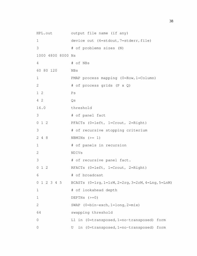
38
HPL.out output file name (if any)
1 device out (6=stdout,7=stderr,file)
3 # of problems sizes (N)
1000 4800 8000 Ns
4 # of NBs
60 80 120 NBs
1 PMAP process mapping (0=Row,1=Column)
2 # of process grids (P x Q)
1 2 Ps
4 2 Qs
16.0 threshold
3 # of panel fact
0 1 2 PFACTs (0=left, 1=Crout, 2=Right)
3 # of recursive stopping criterium
2 4 8 NBMINs (>= 1)
1 # of panels in recursion
2 NDIVs
3 # of recursive panel fact.
0 1 2 RFACTs (0=left, 1=Crout, 2=Right)
6 # of broadcast
0 1 2 3 4 5 BCASTs (0=1rg,1=1rM,2=2rg,3=2rM,4=Lng,5=LnM)
1 # of lookahead depth
1 DEPTHs (>=0)
2 SWAP (0=bin-exch,1=long,2=mix)
64 swapping threshold
0 L1 in (0=transposed,1=no-transposed) form
0 U in (0=transposed,1=no-transposed) form
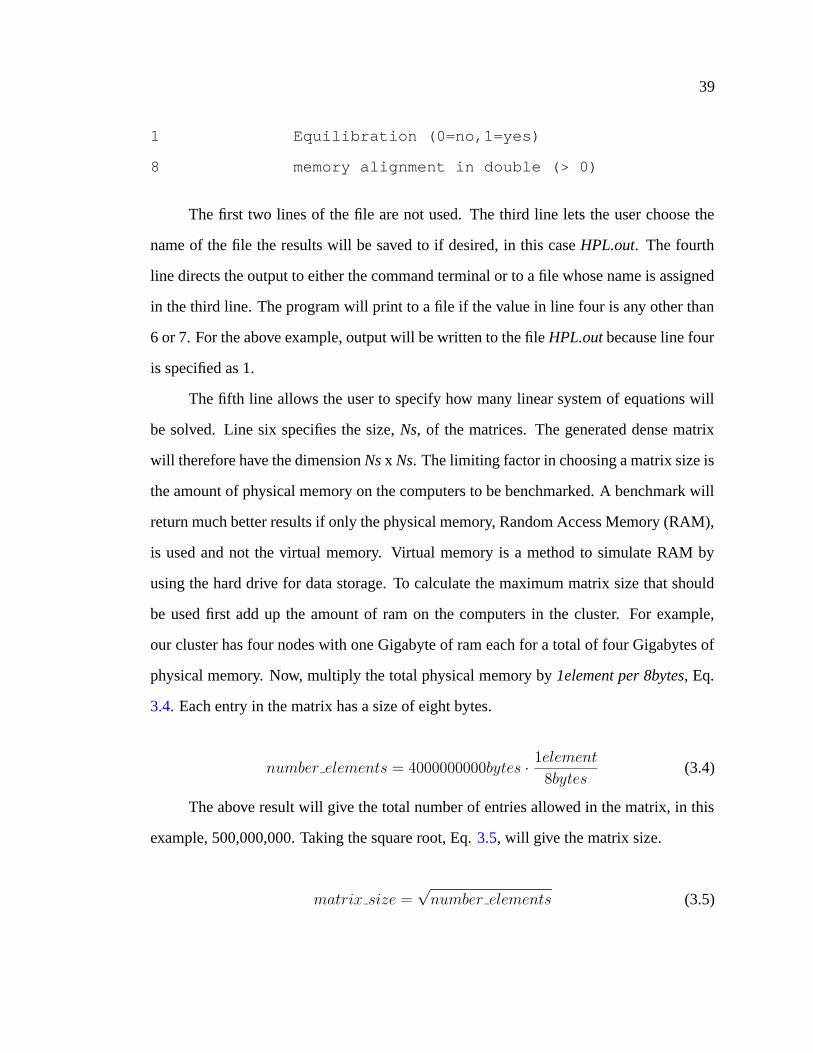
39
1 Equilibration (0=no,1=yes)
8 memory alignment in double (> 0)
The first two lines of the file are not used. The third line lets the user choose the
name of the file the results will be saved to if desired, in this case HPL.out. The fourth
line directs the output to either the command terminal or to a file whose name is assigned
in the third line. The program will print to a file if the value in line four is any other than
6 or 7. For the above example, output will be written to the file HPL.out because line four
is specified as 1.
The fifth line allows the user to specify how many linear system of equations will
be solved. Line six specifies the size, Ns, of the matrices. The generated dense matrix
will therefore have the dimension Ns x Ns. The limiting factor in choosing a matrix size is
the amount of physical memory on the computers to be benchmarked. A benchmark will
return much better results if only the physical memory, Random Access Memory (RAM),
is used and not the virtual memory. Virtual memory is a method to simulate RAM by
using the hard drive for data storage. To calculate the maximum matrix size that should
be used first add up the amount of ram on the computers in the cluster. For example,
our cluster has four nodes with one Gigabyte of ram each for a total of four Gigabytes of
physical memory. Now, multiply the total physical memory by 1element per 8bytes, Eq.
3.4. Each entry in the matrix has a size of eight bytes.
number elements = 4000000000bytes ·1element
8bytes(3.4)
The above result will give the total number of entries allowed in the matrix, in this
example, 500,000,000. Taking the square root, Eq. 3.5, will give the matrix size.
matrix size =√
number elements (3.5)
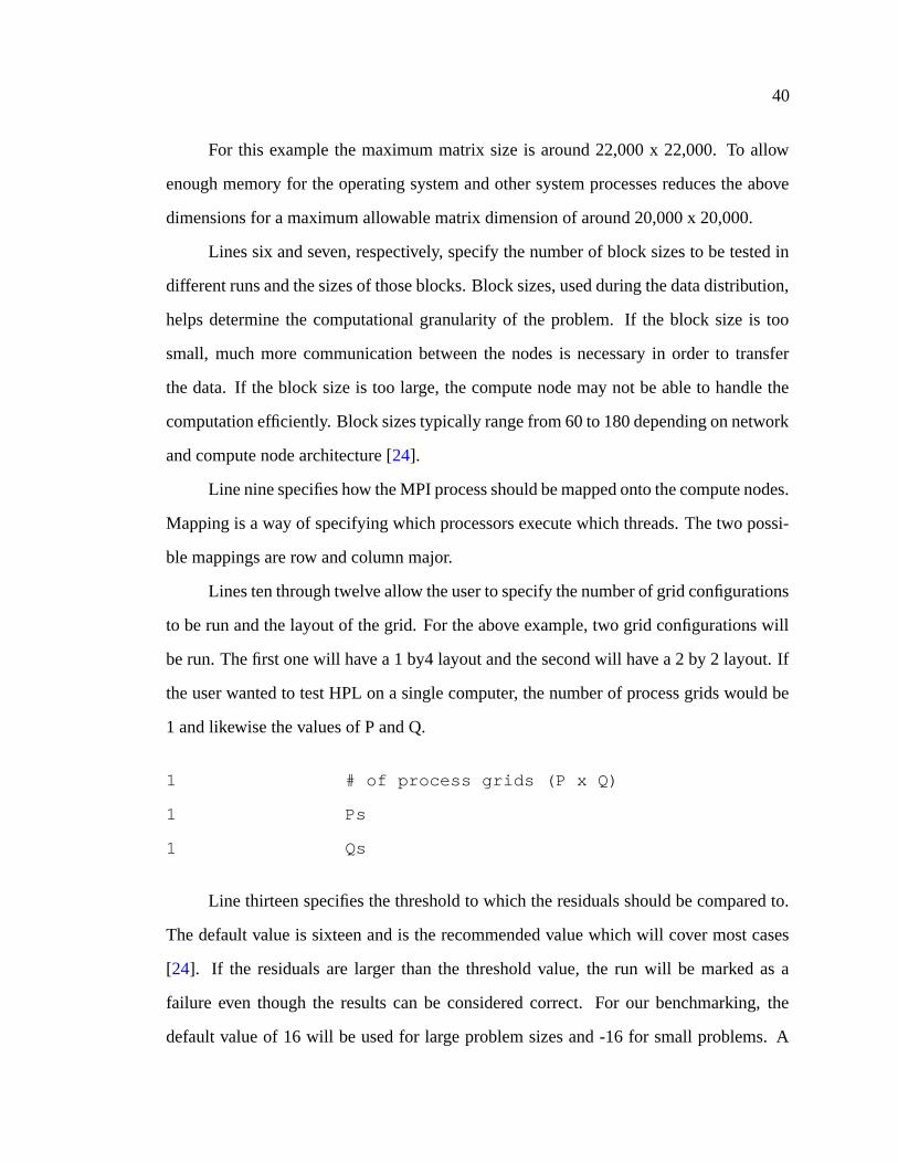
40
For this example the maximum matrix size is around 22,000 x 22,000. To allow
enough memory for the operating system and other system processes reduces the above
dimensions for a maximum allowable matrix dimension of around 20,000 x 20,000.
Lines six and seven, respectively, specify the number of block sizes to be tested in
different runs and the sizes of those blocks. Block sizes, used during the data distribution,
helps determine the computational granularity of the problem. If the block size is too
small, much more communication between the nodes is necessary in order to transfer
the data. If the block size is too large, the compute node may not be able to handle the
computation efficiently. Block sizes typically range from 60 to 180 depending on network
and compute node architecture [24].
Line nine specifies how the MPI process should be mapped onto the compute nodes.
Mapping is a way of specifying which processors execute which threads. The two possi-
ble mappings are row and column major.
Lines ten through twelve allow the user to specify the number of grid configurations
to be run and the layout of the grid. For the above example, two grid configurations will
be run. The first one will have a 1 by4 layout and the second will have a 2 by 2 layout. If
the user wanted to test HPL on a single computer, the number of process grids would be
1 and likewise the values of P and Q.
1 # of process grids (P x Q)
1 Ps
1 Qs
Line thirteen specifies the threshold to which the residuals should be compared to.
The default value is sixteen and is the recommended value which will cover most cases
[24]. If the residuals are larger than the threshold value, the run will be marked as a
failure even though the results can be considered correct. For our benchmarking, the
default value of 16 will be used for large problem sizes and -16 for small problems. A
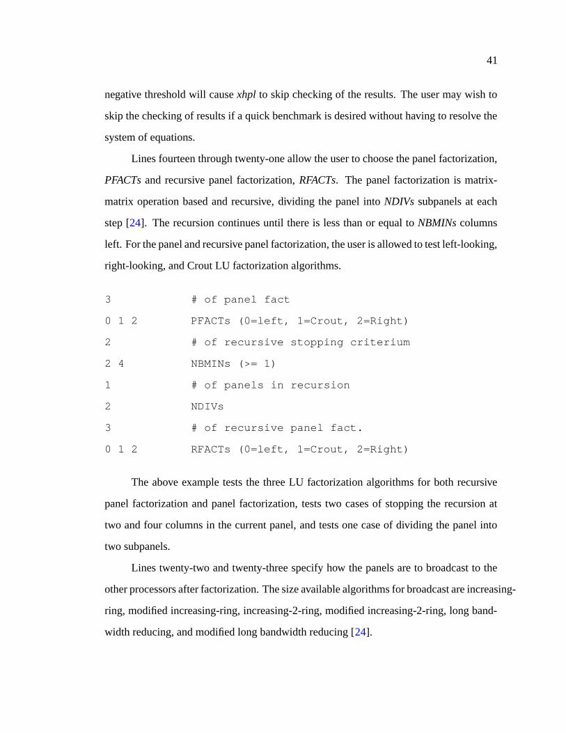
41
negative threshold will cause xhpl to skip checking of the results. The user may wish to
skip the checking of results if a quick benchmark is desired without having to resolve the
system of equations.
Lines fourteen through twenty-one allow the user to choose the panel factorization,
PFACTs and recursive panel factorization, RFACTs. The panel factorization is matrix-
matrix operation based and recursive, dividing the panel into NDIVs subpanels at each
step [24]. The recursion continues until there is less than or equal to NBMINs columns
left. For the panel and recursive panel factorization, the user is allowed to test left-looking,
right-looking, and Crout LU factorization algorithms.
3 # of panel fact
0 1 2 PFACTs (0=left, 1=Crout, 2=Right)
2 # of recursive stopping criterium
2 4 NBMINs (>= 1)
1 # of panels in recursion
2 NDIVs
3 # of recursive panel fact.
0 1 2 RFACTs (0=left, 1=Crout, 2=Right)
The above example tests the three LU factorization algorithms for both recursive
panel factorization and panel factorization, tests two cases of stopping the recursion at
two and four columns in the current panel, and tests one case of dividing the panel into
two subpanels.
Lines twenty-two and twenty-three specify how the panels are to broadcast to the
other processors after factorization. The size available algorithms for broadcast are increasing-
ring, modified increasing-ring, increasing-2-ring, modified increasing-2-ring, long band-
width reducing, and modified long bandwidth reducing [24].
42
The remaining lines specifies options that will further optimize the benchmark tests.
For our runs the recommended values will be used. A further explanation of what the
remaining options can be found at the HPL website [24].
3.3.8 Test Setup
Many tests were conducted with different parameters specified in the file HPL.dat.
Initially, a small problem size, Ns, was tested while varying the other options. From
there it was determined what options allowed xhpl to perform the best. A small problem
size was used primarily because it would take a lot of time to conduct all the tests if a
large size was used. If 5 block sizes, NBs, all 6 panel broadcast methods, BCASTs, and 2
process grids were tested, that would be 60 tests. Even though by using a small problem
size the reported Gflops will not be the highest that is attainable, we still are able to
determine what parameters affect relative performance. After a test with a small problem
size was conducted, the options that performed the worst were eliminated and tests with
the remaining good performing options were carried out. This process of eliminating the
worst performing options and rerunning the tests with the best options was continued until
a set of options that performed the best was obtained.
The first test conducted involved a problem size, Ns, of 1000 on apollo. Initially
only apollo will be tested to get a base measurement for a nodes performance. After
apollo is fully tested, two, then three, then all the nodes will be tested so that the scal-
ability of the cluster can be determined. The HPL.dat file that was used for the initial
testing of apollo is seen in Appendix B.3.2. Six block sizes, left-looking, right-looking
and Crout’s method for factorization, three values for the number of subpanels to create,
and four values for the columns when recursive panel factorization stops. It should be
noted that the threshold used for these tests will be -16. By using a negative threshold,
checking of the results will not be performed. For larger tests and tests using the network,
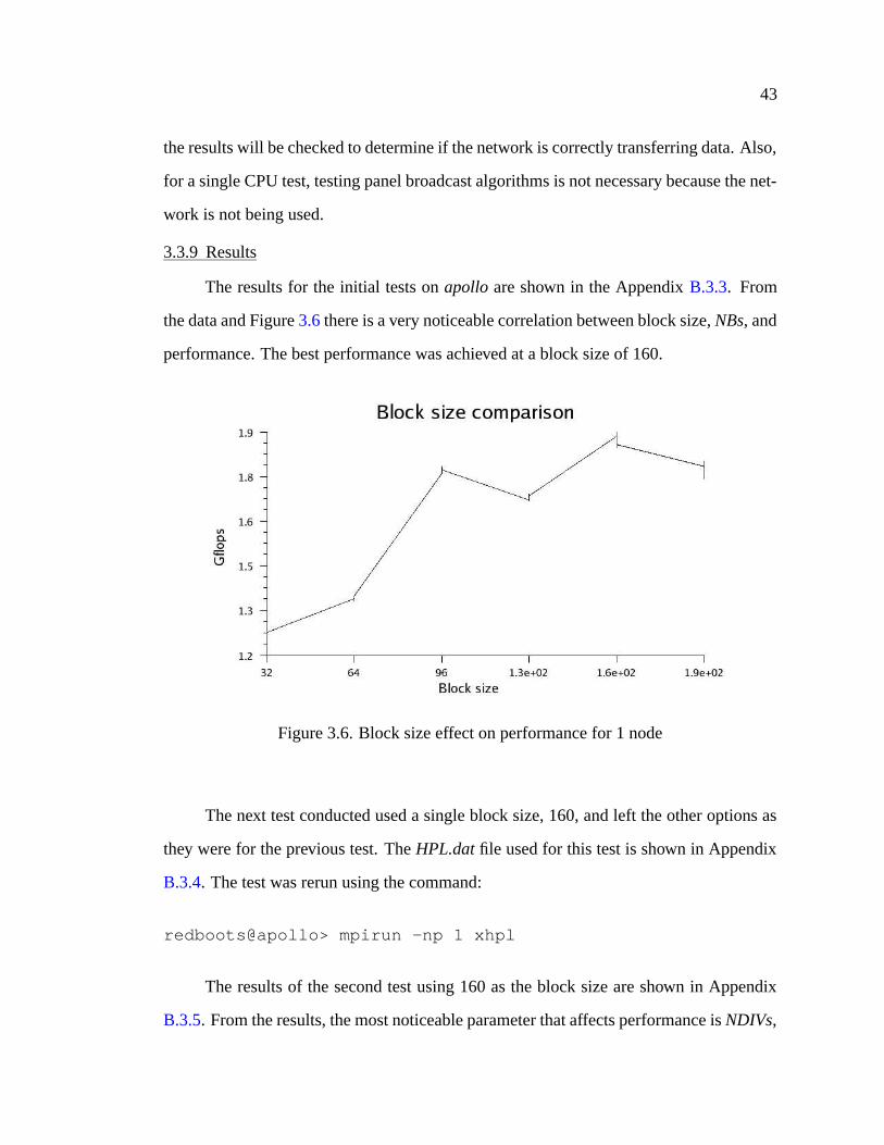
43
the results will be checked to determine if the network is correctly transferring data. Also,
for a single CPU test, testing panel broadcast algorithms is not necessary because the net-
work is not being used.
3.3.9 Results
The results for the initial tests on apollo are shown in the Appendix B.3.3. From
the data and Figure 3.6 there is a very noticeable correlation between block size, NBs, and
performance. The best performance was achieved at a block size of 160.
Figure 3.6. Block size effect on performance for 1 node
The next test conducted used a single block size, 160, and left the other options as
they were for the previous test. The HPL.dat file used for this test is shown in Appendix
B.3.4. The test was rerun using the command:
redboots@apollo> mpirun -np 1 xhpl
The results of the second test using 160 as the block size are shown in Appendix
B.3.5. From the results, the most noticeable parameter that affects performance is NDIVs,
44
or the number of subpanels that are created during the recursive factorization. For NDIVs
equal to 2, the average Gflops is 1.891, for NDIVs equal to 3, the average Gflops is 1.861,
and for a NDIVs equal to 4, the average Gflops is 1.864.
The next test involved setting NDIVs to 2 and rerunning with the other parameters
unchanged. From the data, the parameter that affects performance the most for this run
is the value of NBMINs. A NBMINs value of 4 returns the bests results with an average
of 1.899 Gflops compared to an average of 1.879 Gflops for NBMINs equal to 1, 1.891
Gflops for NBMINs equal to 2, and 1.892 Gflops for NBMINs equal to 8.
The remaining parameters that can be changed are the algorithms used for the panel
factorization and recursive panel factorization. For this test, NBMINs was set to 4 and
rerun. This test was run as before.
redboots@apollo> mpirun -np 1 xhpl
From the results, using any of the algorithms for panel factorization and recursive
panel factorization produced very similar results. Since the three factorization algorithms
produced similar results, for the final test using a large problem size, Crout’s algorithm for
both factorizations will be used mainly because the algorithm implemented in SPOOLES
for factorization is Crout’s.
The final test involving one processor will use the optimum parameters determined
as shown above and also the maximum problem size allowed by system memory. Check-
ing of the solution will also be enable by changing the threshold value, line 13, to a
positive 16. To calculate the maximum problem size, Eqs. 3.4 and 3.5 will be used.
number elements = 1000000000bytes ·1element
8bytes
matrix size =√
125000000
matrix size = 11180
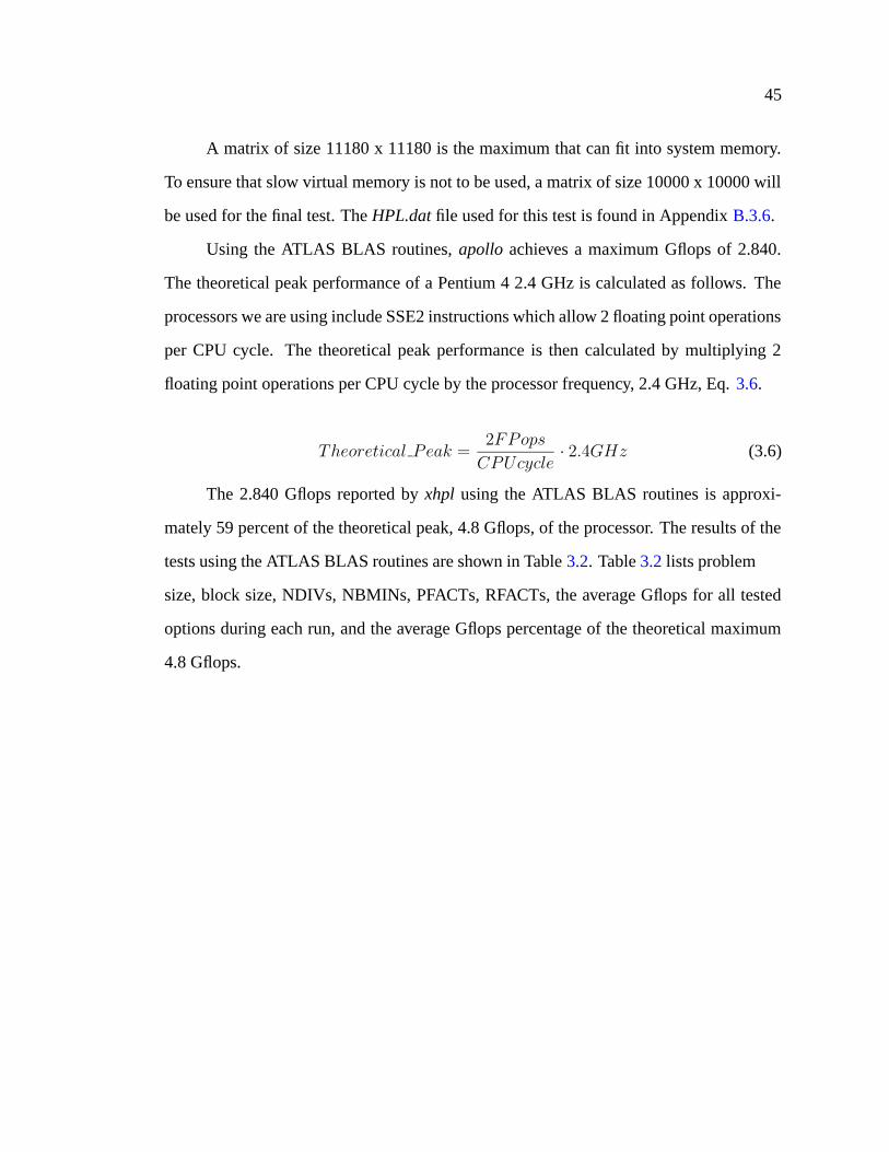
45
A matrix of size 11180 x 11180 is the maximum that can fit into system memory.
To ensure that slow virtual memory is not to be used, a matrix of size 10000 x 10000 will
be used for the final test. The HPL.dat file used for this test is found in Appendix B.3.6.
Using the ATLAS BLAS routines, apollo achieves a maximum Gflops of 2.840.
The theoretical peak performance of a Pentium 4 2.4 GHz is calculated as follows. The
processors we are using include SSE2 instructions which allow 2 floating point operations
per CPU cycle. The theoretical peak performance is then calculated by multiplying 2
floating point operations per CPU cycle by the processor frequency, 2.4 GHz, Eq. 3.6.
Theoretical Peak =2FPops
CPUcycle· 2.4GHz (3.6)
The 2.840 Gflops reported by xhpl using the ATLAS BLAS routines is approxi-
mately 59 percent of the theoretical peak, 4.8 Gflops, of the processor. The results of the
tests using the ATLAS BLAS routines are shown in Table 3.2. Table 3.2 lists problem
size, block size, NDIVs, NBMINs, PFACTs, RFACTs, the average Gflops for all tested
options during each run, and the average Gflops percentage of the theoretical maximum
4.8 Gflops.
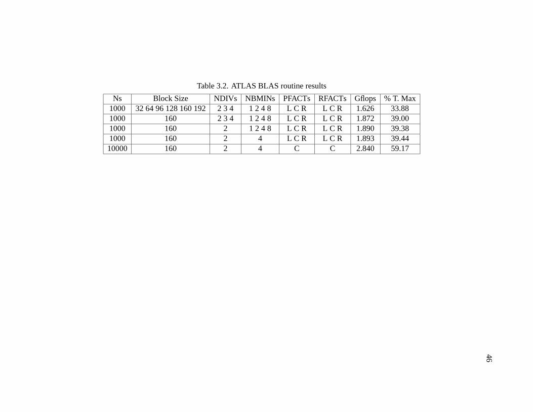
46
Table 3.2. ATLAS BLAS routine results
Ns Block Size NDIVs NBMINs PFACTs RFACTs Gflops % T. Max1000 32 64 96 128 160 192 2 3 4 1 2 4 8 L C R L C R 1.626 33.881000 160 2 3 4 1 2 4 8 L C R L C R 1.872 39.001000 160 2 1 2 4 8 L C R L C R 1.890 39.381000 160 2 4 L C R L C R 1.893 39.4410000 160 2 4 C C 2.840 59.17
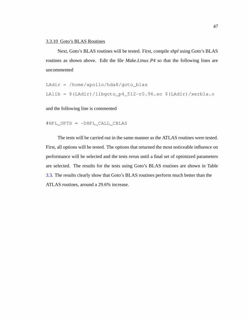
47
3.3.10 Goto’s BLAS Routines
Next, Goto’s BLAS routines will be tested. First, compile xhpl using Goto’s BLAS
routines as shown above. Edit the file Make.Linux P4 so that the following lines are
uncommented
LAdir = /home/apollo/hda8/goto_blas
LAlib = $(LAdir)/libgoto_p4_512-r0.96.so $(LAdir)/xerbla.o
and the following line is commented
#HPL_OPTS = -DHPL_CALL_CBLAS
The tests will be carried out in the same manner as the ATLAS routines were tested.
First, all options will be tested. The options that returned the most noticeable influence on
performance will be selected and the tests rerun until a final set of optimized parameters
are selected. The results for the tests using Goto’s BLAS routines are shown in Table
3.3. The results clearly show that Goto’s BLAS routines perform much better than the
ATLAS routines, around a 29.6% increase.
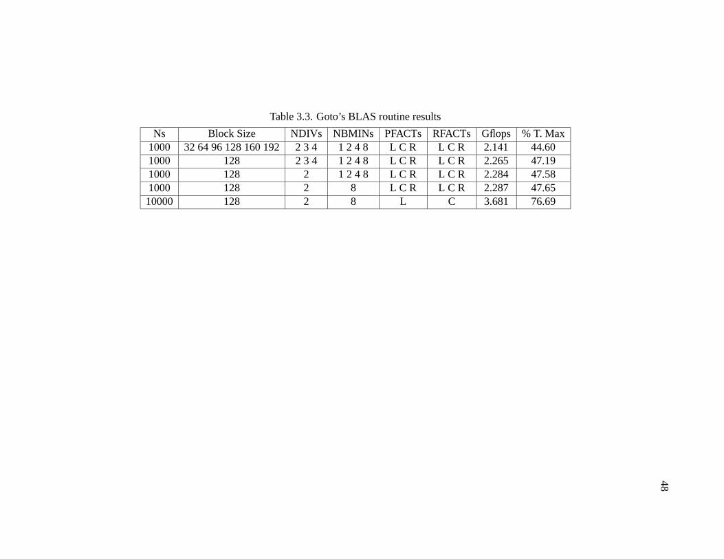
48
Table 3.3. Goto’s BLAS routine results
Ns Block Size NDIVs NBMINs PFACTs RFACTs Gflops % T. Max1000 32 64 96 128 160 192 2 3 4 1 2 4 8 L C R L C R 2.141 44.601000 128 2 3 4 1 2 4 8 L C R L C R 2.265 47.191000 128 2 1 2 4 8 L C R L C R 2.284 47.581000 128 2 8 L C R L C R 2.287 47.6510000 128 2 8 L C 3.681 76.69
49
3.4 HPL–Multiple Node Tests
For this section, multiple nodes will be used. By knowing apollo’s performance,
running xhpl on more than one node will allow us to see the scalability of our cluster.
Ideally, a clusters performance should scale linearly to the number of nodes present. For
example, apollo achieved a maximum Gflops of 3.681 using Goto’s BLAS routines. How-
ever, because of network induced overhead, adding another identical node to the cluster
will not increase the performance to 7.362 Gflops. By determining how scalable a cluster
is, it is possible to select the appropriate cluster configuration for a particular problem
size.
3.4.1 Two Processor Tests
For tests using more than one node, the initial matrix size tested will be increased
from that of the matrix tested in the single node runs. The reasoning behind this is illus-
trated in the tests of MPICH after it was installed. When running cpi, for small problem
sizes a single processor performed better than a multi-node run. By using a small prob-
lem size and multiple nodes, the network would add significant overhead, so much that
it would be difficult to accurately measure the clusters performance. For small problem
sizes, the full potential of a processor isn’t being used, instead time is wasted on inter-
processor communication.
For testing multiple nodes, two other options are added to those tested for a single
node, these being the process grid and panel broadcast algorithm. If these options were
added to the options tested for a single node, this would bring the total number of initial
tests to almost eight-thousand. Instead of running all tests at once, the process grid layout
and panel broadcast algorithms will be tested separately. Once it is determined which
parameters for the process grid layout and panel broadcast perform the best for a general
problem regardless of the other options, the same testing methodology applied to a single
node can be applied to multiple nodes.
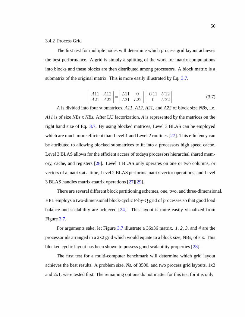
50
3.4.2 Process Grid
The first test for multiple nodes will determine which process grid layout achieves
the best performance. A grid is simply a splitting of the work for matrix computations
into blocks and these blocks are then distributed among processors. A block matrix is a
submatrix of the original matrix. This is more easily illustrated by Eq. 3.7.
A11 A12A21 A22
=L11 0L21 L22
·U11 U120 U22
(3.7)
A is divided into four submatrices, A11, A12, A21, and A22 of block size NBs, i.e.
A11 is of size NBs x NBs. After LU factorization, A is represented by the matrices on the
right hand size of Eq. 3.7. By using blocked matrices, Level 3 BLAS can be employed
which are much more efficient than Level 1 and Level 2 routines [27]. This efficiency can
be attributed to allowing blocked submatrices to fit into a processors high speed cache.
Level 3 BLAS allows for the efficient access of todays processors hierarchal shared mem-
ory, cache, and registers [28]. Level 1 BLAS only operates on one or two columns, or
vectors of a matrix at a time, Level 2 BLAS performs matrix-vector operations, and Level
3 BLAS handles matrix-matrix operations [27][29].
There are several different block partitioning schemes, one, two, and three-dimensional.
HPL employs a two-dimensional block-cyclic P-by-Q grid of processes so that good load
balance and scalability are achieved [24]. This layout is more easily visualized from
Figure 3.7.
For arguments sake, let Figure 3.7 illustrate a 36x36 matrix. 1, 2, 3, and 4 are the
processor ids arranged in a 2x2 grid which would equate to a block size, NBs, of six. This
blocked cyclic layout has been shown to possess good scalability properties [28].
The first test for a multi-computer benchmark will determine which grid layout
achieves the best results. A problem size, Ns, of 3500, and two process grid layouts, 1x2
and 2x1, were tested first. The remaining options do not matter for this test for it is only
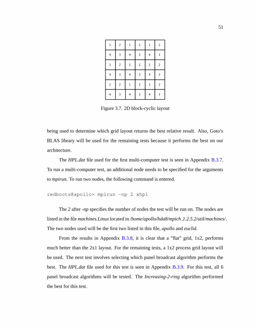
51
Figure 3.7. 2D block-cyclic layout
being used to determine which grid layout returns the best relative result. Also, Goto’s
BLAS library will be used for the remaining tests because it performs the best on our
architecture.
The HPL.dat file used for the first multi-computer test is seen in Appendix B.3.7.
To run a multi-computer test, an additional node needs to be specified for the arguments
to mpirun. To run two nodes, the following command is entered.
redboots@apollo> mpirun -np 2 xhpl
The 2 after -np specifies the number of nodes the test will be run on. The nodes are
listed in the file machines.Linux located in /home/apollo/hda8/mpich 1.2.5.2/util/machines/.
The two nodes used will be the first two listed in this file, apollo and euclid.
From the results in Appendix B.3.8, it is clear that a ”flat” grid, 1x2, performs
much better than the 2x1 layout. For the remaining tests, a 1x2 process grid layout will
be used. The next test involves selecting which panel broadcast algorithm performs the
best. The HPL.dat file used for this test is seen in Appendix B.3.9. For this test, all 6
panel broadcast algorithms will be tested. The Increasing-2-ring algorithm performed
the best for this test.
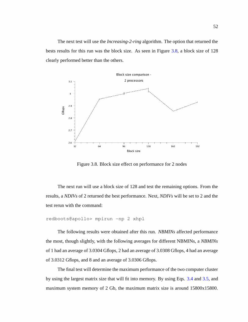
52
The next test will use the Increasing-2-ring algorithm. The option that returned the
bests results for this run was the block size. As seen in Figure 3.8, a block size of 128
clearly performed better than the others.
Figure 3.8. Block size effect on performance for 2 nodes
The next run will use a block size of 128 and test the remaining options. From the
results, a NDIVs of 2 returned the best performance. Next, NDIVs will be set to 2 and the
test rerun with the command:
redboots@apollo> mpirun -np 2 xhpl
The following results were obtained after this run. NBMINs affected performance
the most, though slightly, with the following averages for different NBMINs, a NBMINs
of 1 had an average of 3.0304 Gflops, 2 had an average of 3.0308 Gflops, 4 had an average
of 3.0312 Gflops, and 8 and an average of 3.0306 Gflops.
The final test will determine the maximum performance of the two computer cluster
by using the largest matrix size that will fit into memory. By using Eqs. 3.4 and 3.5, and
maximum system memory of 2 Gb, the maximum matrix size is around 15800x15800.

53
To account for memory to run the operating system, a matrix of size 14500x14500 will
be used. The HPL.dat file used for this test is in Appendix B.3.10. This run achieved
5.085 Gflops. Out of curiosity different matrix sizes were also tested. The results of these
tests are as follows: 13500x13500 achieved 5.245 Gflops, 12500x12500 achieved 5.364
Gflops, and 11500x11500 achieved 5.222 Gflops. The results are summarized in Table
3.4.
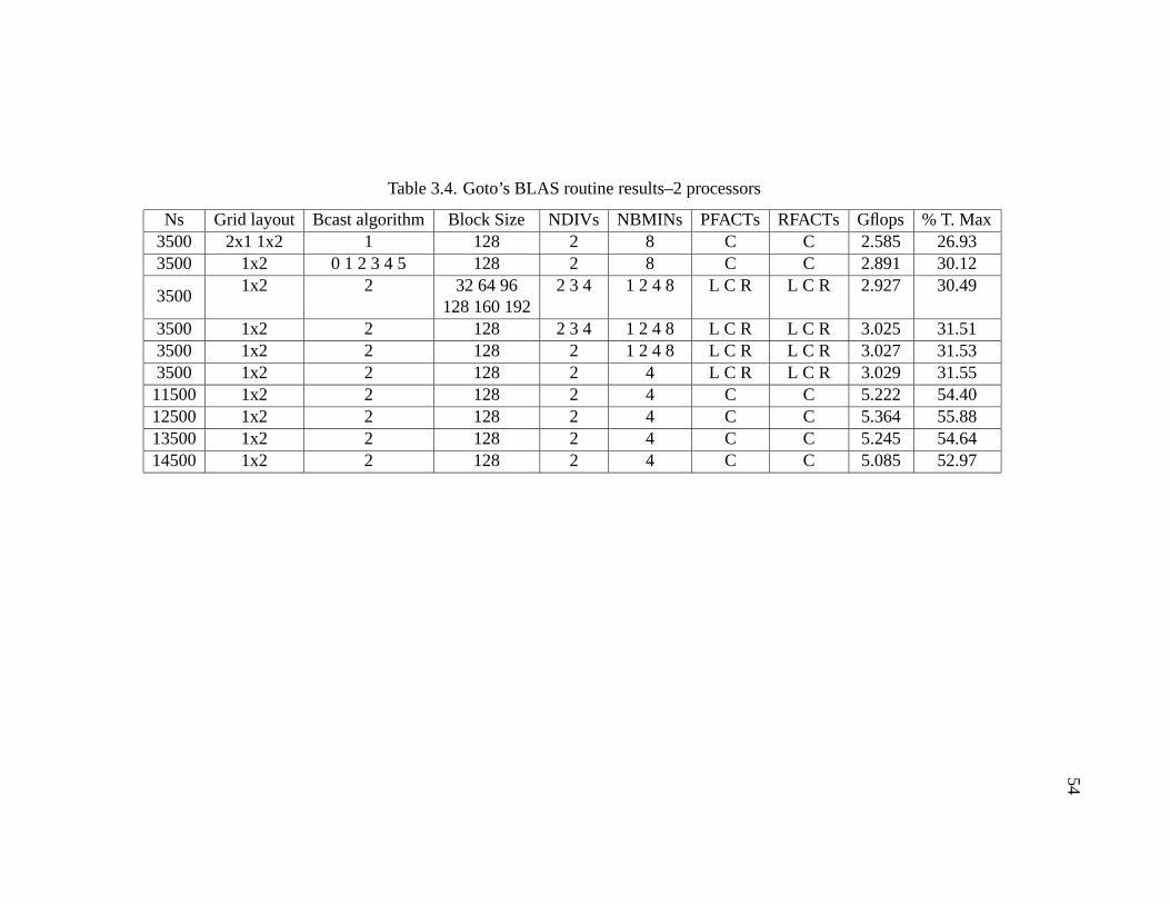
54
Table 3.4. Goto’s BLAS routine results–2 processors
Ns Grid layout Bcast algorithm Block Size NDIVs NBMINs PFACTs RFACTs Gflops % T. Max3500 2x1 1x2 1 128 2 8 C C 2.585 26.933500 1x2 0 1 2 3 4 5 128 2 8 C C 2.891 30.12
35001x2 2 32 64 96 2 3 4 1 2 4 8 L C R L C R 2.927 30.49
128 160 1923500 1x2 2 128 2 3 4 1 2 4 8 L C R L C R 3.025 31.513500 1x2 2 128 2 1 2 4 8 L C R L C R 3.027 31.533500 1x2 2 128 2 4 L C R L C R 3.029 31.5511500 1x2 2 128 2 4 C C 5.222 54.4012500 1x2 2 128 2 4 C C 5.364 55.8813500 1x2 2 128 2 4 C C 5.245 54.6414500 1x2 2 128 2 4 C C 5.085 52.97
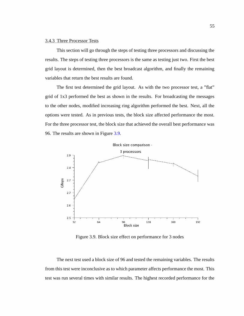
55
3.4.3 Three Processor Tests
This section will go through the steps of testing three processors and discussing the
results. The steps of testing three processors is the same as testing just two. First the best
grid layout is determined, then the best broadcast algorithm, and finally the remaining
variables that return the best results are found.
The first test determined the grid layout. As with the two processor test, a ”flat”
grid of 1x3 performed the best as shown in the results. For broadcasting the messages
to the other nodes, modified increasing ring algorithm performed the best. Next, all the
options were tested. As in previous tests, the block size affected performance the most.
For the three processor test, the block size that achieved the overall best performance was
96. The results are shown in Figure 3.9.
Figure 3.9. Block size effect on performance for 3 nodes
The next test used a block size of 96 and tested the remaining variables. The results
from this test were inconclusive as to which parameter affects performance the most. This
test was run several times with similar results. The highest recorded performance for the

56
test was 2.853 Gflops which occurred four times. Since no conclusion could be made
from the results, the remaining variables were chosen to be Crout’s algorithm for both the
panel factorization and panel factorization, NBMINs of 4, and NDIVs of 2.
The final test will determine the maximum performance of our three node cluster.
To determine the maximum matrix size to use, Eqs. 3.4 and 3.5 will be used. For three
gigabytes of total system memory and accounting for operating system memory require-
ments, a maximum matrix size of 17800x17800 will be used. As with the two processor
tests, different matrix sizes will be tested to see which achieves maximum performance.
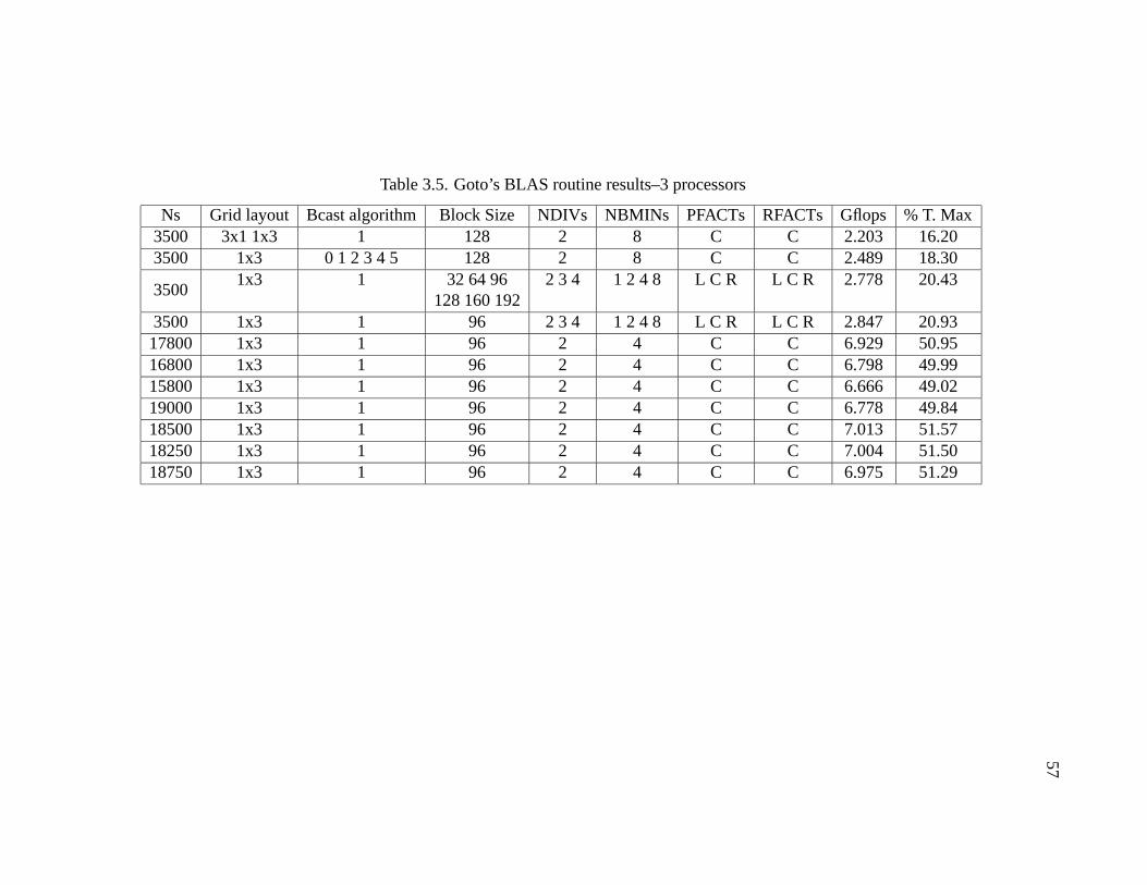
57
Table 3.5. Goto’s BLAS routine results–3 processors
Ns Grid layout Bcast algorithm Block Size NDIVs NBMINs PFACTs RFACTs Gflops % T. Max3500 3x1 1x3 1 128 2 8 C C 2.203 16.203500 1x3 0 1 2 3 4 5 128 2 8 C C 2.489 18.30
35001x3 1 32 64 96 2 3 4 1 2 4 8 L C R L C R 2.778 20.43
128 160 1923500 1x3 1 96 2 3 4 1 2 4 8 L C R L C R 2.847 20.9317800 1x3 1 96 2 4 C C 6.929 50.9516800 1x3 1 96 2 4 C C 6.798 49.9915800 1x3 1 96 2 4 C C 6.666 49.0219000 1x3 1 96 2 4 C C 6.778 49.8418500 1x3 1 96 2 4 C C 7.013 51.5718250 1x3 1 96 2 4 C C 7.004 51.5018750 1x3 1 96 2 4 C C 6.975 51.29
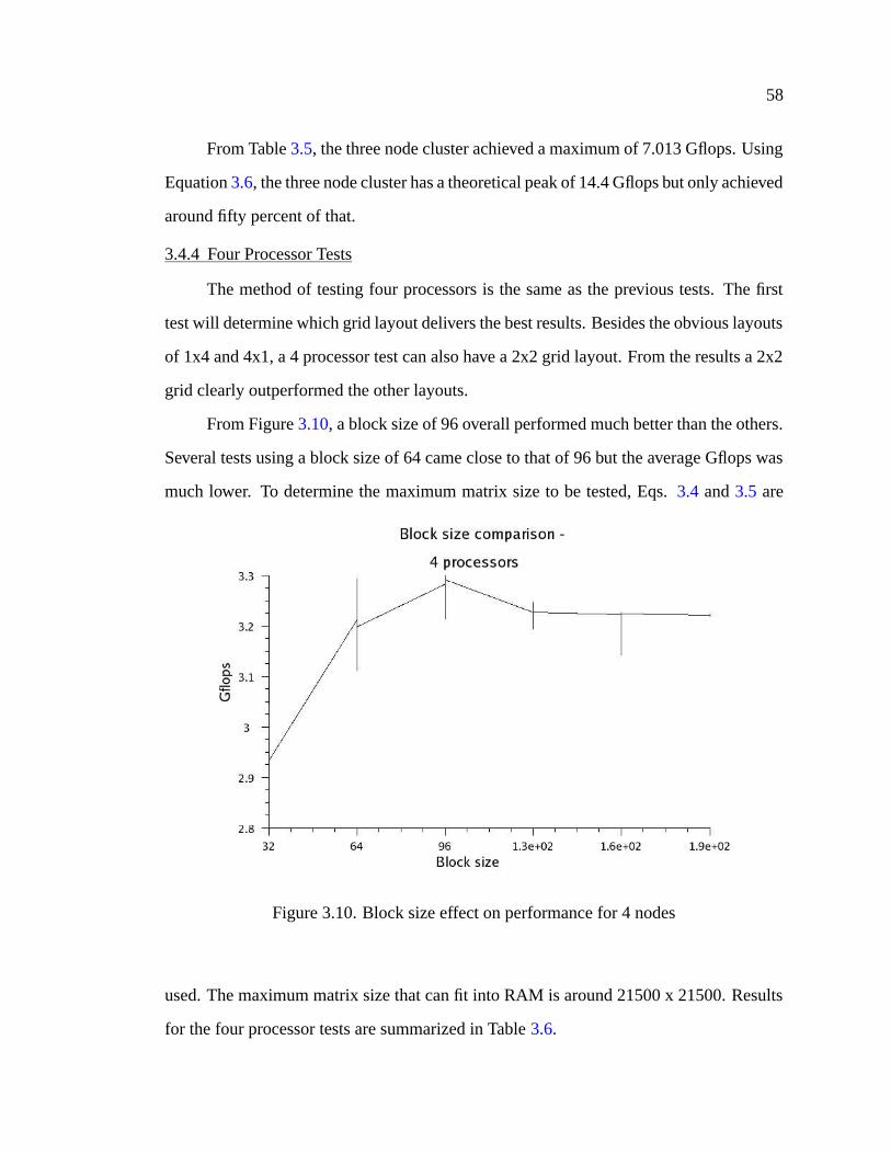
58
From Table 3.5, the three node cluster achieved a maximum of 7.013 Gflops. Using
Equation 3.6, the three node cluster has a theoretical peak of 14.4 Gflops but only achieved
around fifty percent of that.
3.4.4 Four Processor Tests
The method of testing four processors is the same as the previous tests. The first
test will determine which grid layout delivers the best results. Besides the obvious layouts
of 1x4 and 4x1, a 4 processor test can also have a 2x2 grid layout. From the results a 2x2
grid clearly outperformed the other layouts.
From Figure 3.10, a block size of 96 overall performed much better than the others.
Several tests using a block size of 64 came close to that of 96 but the average Gflops was
much lower. To determine the maximum matrix size to be tested, Eqs. 3.4 and 3.5 are
Figure 3.10. Block size effect on performance for 4 nodes
used. The maximum matrix size that can fit into RAM is around 21500 x 21500. Results
for the four processor tests are summarized in Table 3.6.
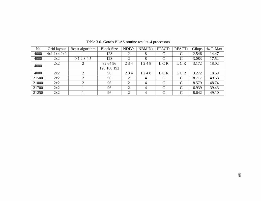
59
Table 3.6. Goto’s BLAS routine results–4 processors
Ns Grid layout Bcast algorithm Block Size NDIVs NBMINs PFACTs RFACTs Gflops % T. Max4000 4x1 1x4 2x2 1 128 2 8 C C 2.546 14.474000 2x2 0 1 2 3 4 5 128 2 8 C C 3.083 17.52
40002x2 2 32 64 96 2 3 4 1 2 4 8 L C R L C R 3.172 18.02
128 160 1924000 2x2 2 96 2 3 4 1 2 4 8 L C R L C R 3.272 18.5921500 2x2 2 96 2 4 C C 8.717 49.5321000 2x2 2 96 2 4 C C 8.579 48.7421700 2x2 1 96 2 4 C C 6.939 39.4321250 2x2 1 96 2 4 C C 8.642 49.10

60
3.4.5 Conclusions
Several conclusions can be made from the benchmarking tests. First, from the
HPL test results, there is a strong correlation between software optimized for a particu-
lar processor architecture and its performance. Clearly, the BLAS routines provided by
Kazushige Goto with optimizations for a processors cache outperform the optimized AT-
LAS routines by as much as 29%. While no changes will be made to the algorithm used
by SPOOLES to solve linear equations, there is always room for improvement in compu-
tational software. The ATLAS routines were long considered the best BLAS library until
Goto’s routines made further improvements.
From Figure 3.11, another important point is illustrated. As the number of proces-
sors increases and depending on the problem type, the actual maximum performance of
a cluster when compared to the theoretical performance generally decreases as the num-
ber of processors increases [6]. As the number of processors increase, so does the time
for each compute note to intercommunicate and share data. If a cluster was only able
to reach a small percentage of its theoretical peak, there may be an underlying problem
with the network or compute node setup. If the cluster is used to solve communication
intensive problems the network may require Gigabit Ethernet or a proprietary network
that is designed for low latency and high bandwidth. On the other hand, if the problems
are computational intensive, increasing the RAM or processor speed ares two possible so-
lutions. Although the performance ratio decreases as the nodes increases, the advantage
of using more nodes is that the maximum problem size that can be solved increases. A
problem size of 12000x12000 was tested under one processor and took around two and
a half hours with the virtual memory being used extensively. Using four processors, the
same problem size was solved in less than three minutes with no virtual memory being
used. Although the solve efficiency of using multiple processors is less than that of one
processor, by spreading the work among compute nodes, large problems can be solved,
although not efficiently, but in a much more reasonable time frame.
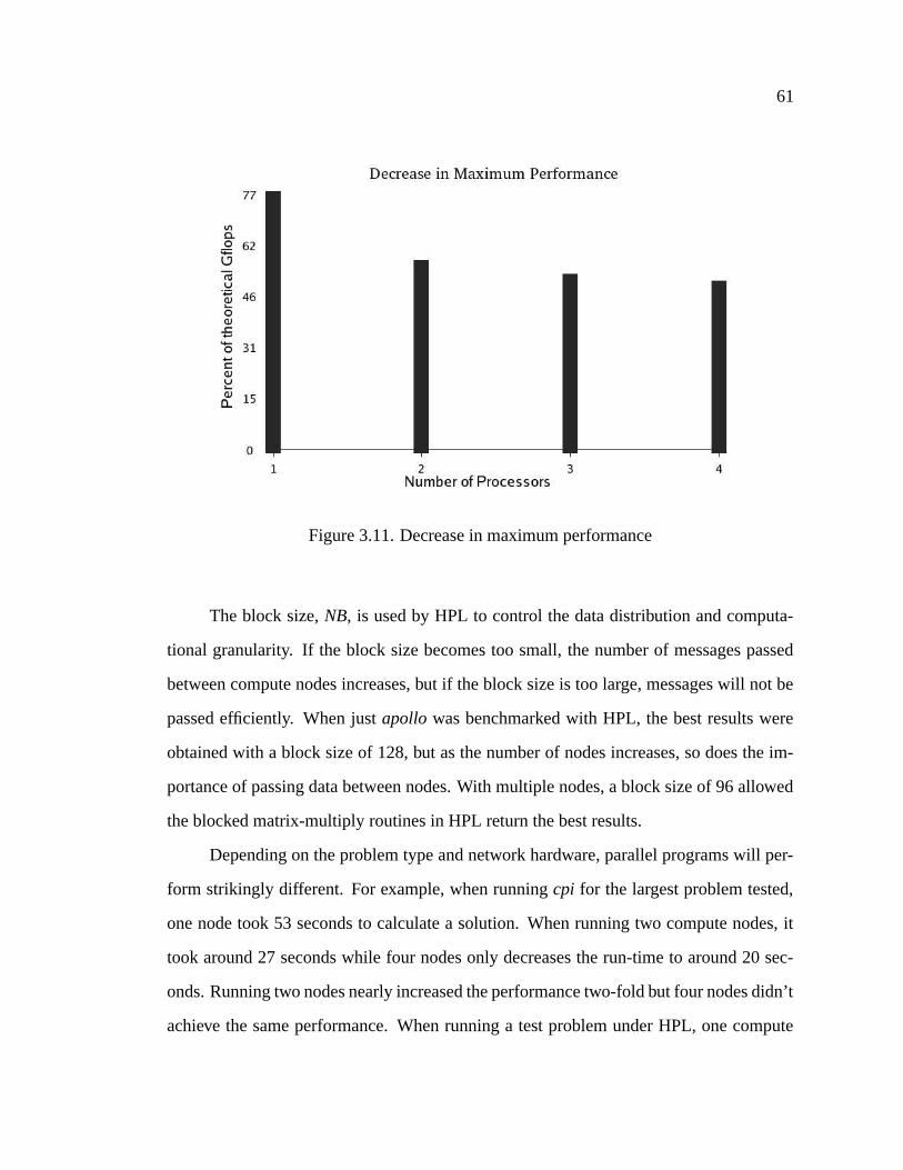
61
Figure 3.11. Decrease in maximum performance
The block size, NB, is used by HPL to control the data distribution and computa-
tional granularity. If the block size becomes too small, the number of messages passed
between compute nodes increases, but if the block size is too large, messages will not be
passed efficiently. When just apollo was benchmarked with HPL, the best results were
obtained with a block size of 128, but as the number of nodes increases, so does the im-
portance of passing data between nodes. With multiple nodes, a block size of 96 allowed
the blocked matrix-multiply routines in HPL return the best results.
Depending on the problem type and network hardware, parallel programs will per-
form strikingly different. For example, when running cpi for the largest problem tested,
one node took 53 seconds to calculate a solution. When running two compute nodes, it
took around 27 seconds while four nodes only decreases the run-time to around 20 sec-
onds. Running two nodes nearly increased the performance two-fold but four nodes didn’t
achieve the same performance. When running a test problem under HPL, one compute

62
node completed a run in three minutes for a problem size of 10000x10000, two compute
nodes completed the same test run in two minutes and fifteen seconds while four nodes
took one minute forty-nine seconds. For computational intensive problems such as those
solving linear system of equations, a fast network is critical to achieving good scalability.
For problems that just divide up the work and send it to the compute nodes without a lot
of interprocessor communication like cpi, a fast network isn’t as important to achieving
acceptable speedup.
CHAPTER 4CALCULIX
CalculiX [30] is an Open Source software package that provides the tools to create
two-dimensional and three-dimensional geometry, create a mesh out of the geometry,
apply boundary conditions and loadings, and then solve the problem. CalculiX is free
software, can be redistributed and/or modified under the terms of the GNU General Public
License [31]. CalculiX was developed by a team at MTU AeroEngines in their spare time
and were granted permission to publish their work.
4.1 Installation of CalculiX GraphiX
There are two separate programs that make up CalculiX: cgx (CalculiX GraphiX)
and ccx (CalculiX CrunchiX). cgx is the graphical pre-processor that creates the geometry
and finite-element mesh and post-processor which views the results. ccx is the solver that
calculates the displacement or temperature of the nodes.
First go to http://www.dhondt.de/ and scroll to near the bottom of the page. Se-
lect the link under Available downloads for the graphical interface (CalculiX GraphiX:
cgx): that reads a statically link Linux binary. Save the file to a folder, in our case
/home/apollo/hda8. Unzip the file by typing:
redboots@apollo> gunzip cgx_1.1.exe.tar.gz
redboots@apollo> tar -xvf cgx_1.1.exe.tar’
This will create the file cgx 1.1.exe. Rename the file cgx 1.1.exe to cgx, become
root, move the file to /usr/local/bin and make it executable.
redboots@apollo> mv cgx_1.1.exe cgx
redboots@apollo> su
63
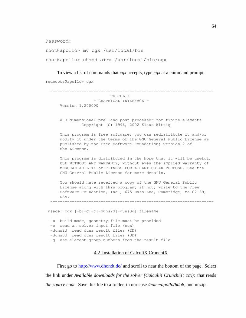
64
Password:
root@apollo> mv cgx /usr/local/bin
root@apollo> chmod a+rx /usr/local/bin/cgx
To view a list of commands that cgx accepts, type cgx at a command prompt.
redboots@apollo> cgx
--------------------------------------------------------------------CALCULIX
- GRAPHICAL INTERFACE -Version 1.200000
A 3-dimensional pre- and post-processor for finite elementsCopyright (C) 1996, 2002 Klaus Wittig
This program is free software; you can redistribute it and/ormodify it under the terms of the GNU General Public License aspublished by the Free Software Foundation; version 2 ofthe License.
This program is distributed in the hope that it will be useful,but WITHOUT ANY WARRANTY; without even the implied warranty ofMERCHANTABILITY or FITNESS FOR A PARTICULAR PURPOSE. See theGNU General Public License for more details.
You should have received a copy of the GNU General PublicLicense along with this program; if not, write to the FreeSoftware Foundation, Inc., 675 Mass Ave, Cambridge, MA 02139,USA.
--------------------------------------------------------------------
usage: cgx [-b|-g|-c|-duns2d|-duns3d] filename
-b build-mode, geometry file must be provided-c read an solver input file (ccx)-duns2d read duns result files (2D)-duns3d read duns result files (3D)-g use element-group-numbers from the result-file
4.2 Installation of CalculiX CrunchiX
First go to http://www.dhondt.de/ and scroll to near the bottom of the page. Select
the link under Available downloads for the solver (CalculiX CrunchiX: ccx): that reads
the source code. Save this file to a folder, in our case /home/apollo/hda8, and unzip.
65
redboots@apollo> gunzip ccx_1.1.src.tar.gz
redboots@apollo> tar -xvf ccx_1.1.src.tar
This creates the folder CalculiX with the source code inside CalculiX/ccx 1.1/src.
In order to build the serial solver for CalculiX, SPOOLES and ARPACK need to be
installed. ARPACK is a collection of Fortran 77 subroutines designed to solve large scale
eigenvalue problems [32] while SPOOLES provides the solver for sparse, linear systems
of equations [33].
4.2.1 ARPACK Installation
To download and install the ARnoldi PACKage (ARPACK), first go to the home-
page at http://www.caam.rice.edu/software/ARPACK/ and click the link for Download
Software. Download the zipped file arpack96.tar.gz to a directory, in our case
/home/apollo/hda8/, and unpack.
redboots@apollo> gunzip arpack96.tar.gz
redboots@apollo> tar -xvf arpack96.tar
This will create the folder ARPACK. Enclosed in ARPACK is the source code, lo-
cated in SRC, examples, documentation, and several Makefiles for different architectures
located in ARMAKES. Copy the file $ARPACK/ARMAKES/ARmake.SUN4 to the main
ARPACK directory and rename it to ARmake.inc.
redboots@apollo> cp ARMAKES/ARmake.SUN4 ARmake.inc
Edit ARmake.inc so that it points to the main ARPACK directory, the correct Fortran
compiler, and specifies Linux as the platform. The ARmake.inc file used for our system is
located in Appendix C.1. Finally, while in the main ARPACK directory, make the library.
redboots@apollo> make lib
This will create the ARPACK library file libarpack Linux.a in the current directory.
66
4.2.2 SPOOLES Installation
To install the SParse Object Oriented Linear Equations Solver (SPOOLES), first go
to the projects website at
http://www.netlib.org/linalg/spooles/spooles.2.2.html. Near the middle of the webpage,
there are links for documentation and software downloads. Download the file
spooles.2.2.tgz, place it in the folder SPOOLES.2.2, and unpack. The main directory for
SPOOLES is located in /home/apollo/hda8 for our installation.
redboots@apollo> cd /home/apollo/hda8
redboots@apollo> mkdir SPOOLES.2.2
redboots@apollo> mv spooles.2.2.tgz SPOOLES.2.2
redboots@apollo> cd SPOOLES.2.2
redboots@apollo> tar -xvzf spooles.2.2.tgz
This will unpack spooles.2.2.tgz in the folder SPOOLES.2.2. First, edit the file
Make.inc so that it points to the correct compiler, MPICH install location, MPICH li-
braries, and include directory. The MPICH options are only for building the parallel
solver which will be discussed later.
To create the library, while in the directory /home/apollo/hda8/SPOOLES.2.2, type:
redboots@apollo> make lib
This will create the library spooles.a in $SPOOLES.2.2/.
4.2.3 Compile CalculiX CrunchiX
After ARPACK and SPOOLES are installed, enter into the CalculiX CrunchiX
source directory.
redboots@apollo> cd /home/apollo/hda8/CalculiX/ccx_1.1/src
67
Edit the file Makefile so that it points to the ARPACK and SPOOLES main direc-
tories and to their compiled libraries, and also to the correct C and Fortran 77 compilers.
The Makefile used for our setup is seen in Appendix C.2.
After the Makefile has been edited, type:
redboots@apollo> make
This will compile the solver for CalculiX. Now copy the solver, ccx 1.1, to the
/usr/local/bin and make it executable and readable by users.
redboots@apollo> su
Password:
root@apollo> cp ccx_1.1 /usr/local/bin
root@apollo> chmod a+rx /usr/local/bin/ccx_1.1
4.3 Geometric Capabilities
This section describes briefly the steps from creating a model to viewing the results
of a finite-element analysis. The first step is to create a model. For two-dimensional
geometries, points, lines, and surfaces are defined and with three-dimensional geometries,
points, lines, surfaces, and also bodies are defined.
The easiest way to create a point in CalculiX is by defining its location in a three-
dimensional space. Each point can be assigned a name or you use the wild card character
! and let CalculiX name the point for you.
After points, the next geometric entity that is created are lines. Lines can be straight,
an arc, or a spline. To create a straight line 2 points are selected. For an arc, a beginning
and endpoint are selected along with the arcs center point. For a spline, multiple points
are defined and then each point is selected to create the spline.
Surfaces are defined by selecting 3 to 5 lines. By using the command qsur the
68
mouse can be used to select lines and generate surfaces. Surfaces may be flat or curved
depending on the boundary defining lines.
Bodies are defined by 5 to 7 surfaces. After a surface is created, it can be copied
and translated or swept about a trajectory to create a body. Also, bodies can be created
by creating all the necessary surfaces and using the command qbod to select them all and
create the desired body.
4.4 Pre-processing
CalculiX allows for the creation of fairly complex models. Points, lines, surfaces,
and bodies are created, in that order, by either typing them or by using the mouse for
selection through the interface. Another option, since the file format is straightforward,
one can simply write the geometry file directly through your favorite text editor. If a point
is modified, the line that is defined partially by that point will also be modified and all
related surfaces and bodies. This also holds true for modifying lines, surfaces and bodies
and their associated geometric entities.
To begin creating geometry with CalculiX, issue the command:
redboots@apollo> cgx -b all.fbd
where all.fbd is the geometry file being created. This brings up the main screen seen in
Figure 4.1.
Creation of geometric entities can be performed in a multitude of ways as described
in the following.
4.4.1 Points
Points are created by entering its location in three-dimensional space or by the
splitting of lines. To create a point, simply type, while the mouse cursor is within the
CalculiX window, the following:
69
Figure 4.1. Opening screen
pnt p1 0.5 0.2 10
This creates a point named p1 at 0.5 in the x, 0.2 in the y, and 10 in the z-direction.
If the user wanted CalculiX to assign names to points, instead of typing p1, the user would
replace it with !. Instead of using the CalculiX display, the following can be entered in
the file all.fbd to create the same point.
PNT p1 0.50 0.20 10.0
In Figure 4.2 p1 is plotted with its name.
4.4.2 Lines
Lines are created by creating points then selecting these points or by entering a
command. To create a line by selection, at least 2 points must be created. First, enter the
command:
qlin
A little selection box appears. When one of the points is within the selection box
press b for begin and l for line when the selection box is over the second point. b is always
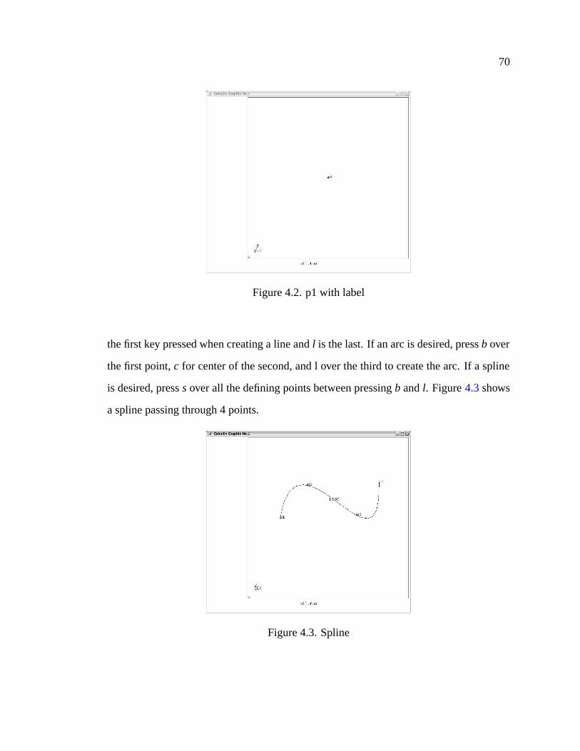
70
Figure 4.2. p1 with label
the first key pressed when creating a line and l is the last. If an arc is desired, press b over
the first point, c for center of the second, and l over the third to create the arc. If a spline
is desired, press s over all the defining points between pressing b and l. Figure 4.3 shows
a spline passing through 4 points.
Figure 4.3. Spline
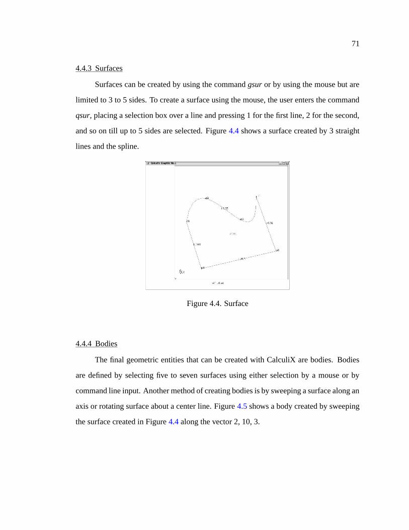
71
4.4.3 Surfaces
Surfaces can be created by using the command gsur or by using the mouse but are
limited to 3 to 5 sides. To create a surface using the mouse, the user enters the command
qsur, placing a selection box over a line and pressing 1 for the first line, 2 for the second,
and so on till up to 5 sides are selected. Figure 4.4 shows a surface created by 3 straight
lines and the spline.
Figure 4.4. Surface
4.4.4 Bodies
The final geometric entities that can be created with CalculiX are bodies. Bodies
are defined by selecting five to seven surfaces using either selection by a mouse or by
command line input. Another method of creating bodies is by sweeping a surface along an
axis or rotating surface about a center line. Figure 4.5 shows a body created by sweeping
the surface created in Figure 4.4 along the vector 2, 10, 3.

72
Figure 4.5. Body created by sweeping
4.5 Finite-Element Mesh Creation
This section describes the finite-element mesh creating capabilities of CalculiX.
CalculiX is able to create and handle several two-dimensional and three-dimensional ele-
ments. Two-dimensional elements that CalculiX can create are:
• 2 node beam element
• 3 node beam element
• 3 node triangular element
• 6 node triangular element
• 4 node shell element
• 8 node shell element
Three-dimensional elements that CalculiX can create are:
• 8 node brick element

73
• 20 node brick element
Although CalculiX can not create other elements at this time, the finite-element
solver is able to handle them and CalculiX can then post-process the results. The three-
dimensional elements that can be solved but not created are:
• 4 node tetrahedral element
• 10 node tetrahedral element
• 6 node wedge element
• 15 node wedge element
After the geometry is created, CalculiX allows the user to create a finite-element
mesh. To create a mesh, the user specifies the number of elements along an edge and then
to create an 8-node brick element, issues the command:
elty all he8
Twenty-node brick elements can be created by simply replacing he8 with he20.
Next, to create the mesh, type:
mesh all
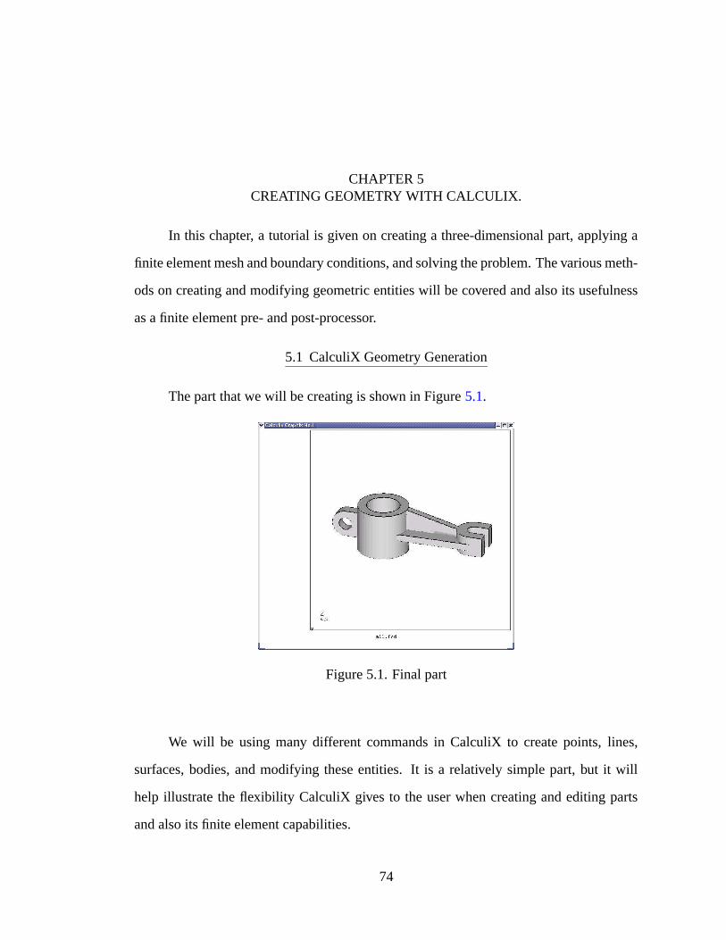
CHAPTER 5CREATING GEOMETRY WITH CALCULIX.
In this chapter, a tutorial is given on creating a three-dimensional part, applying a
finite element mesh and boundary conditions, and solving the problem. The various meth-
ods on creating and modifying geometric entities will be covered and also its usefulness
as a finite element pre- and post-processor.
5.1 CalculiX Geometry Generation
The part that we will be creating is shown in Figure 5.1.
Figure 5.1. Final part
We will be using many different commands in CalculiX to create points, lines,
surfaces, bodies, and modifying these entities. It is a relatively simple part, but it will
help illustrate the flexibility CalculiX gives to the user when creating and editing parts
and also its finite element capabilities.
74
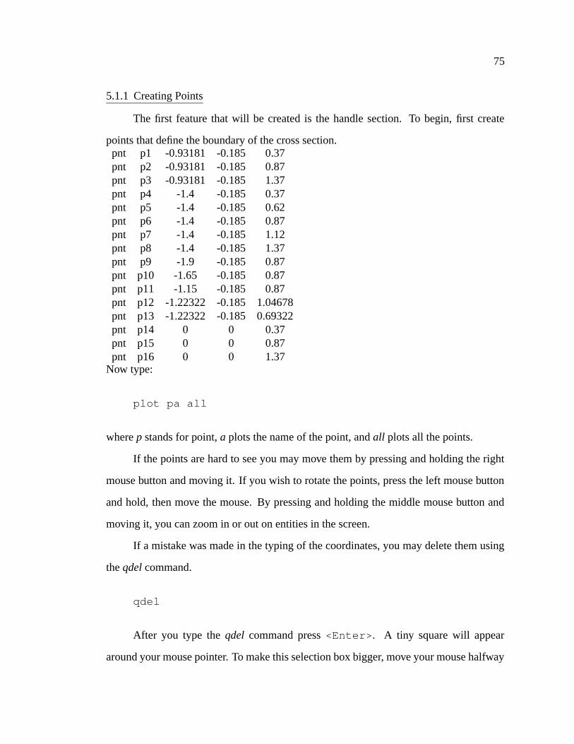
75
5.1.1 Creating Points
The first feature that will be created is the handle section. To begin, first create
points that define the boundary of the cross section.pnt p1 -0.93181 -0.185 0.37pnt p2 -0.93181 -0.185 0.87pnt p3 -0.93181 -0.185 1.37pnt p4 -1.4 -0.185 0.37pnt p5 -1.4 -0.185 0.62pnt p6 -1.4 -0.185 0.87pnt p7 -1.4 -0.185 1.12pnt p8 -1.4 -0.185 1.37pnt p9 -1.9 -0.185 0.87pnt p10 -1.65 -0.185 0.87pnt p11 -1.15 -0.185 0.87pnt p12 -1.22322 -0.185 1.04678pnt p13 -1.22322 -0.185 0.69322pnt p14 0 0 0.37pnt p15 0 0 0.87pnt p16 0 0 1.37
Now type:
plot pa all
where p stands for point, a plots the name of the point, and all plots all the points.
If the points are hard to see you may move them by pressing and holding the right
mouse button and moving it. If you wish to rotate the points, press the left mouse button
and hold, then move the mouse. By pressing and holding the middle mouse button and
moving it, you can zoom in or out on entities in the screen.
If a mistake was made in the typing of the coordinates, you may delete them using
the qdel command.
qdel
After you type the qdel command press <Enter>. A tiny square will appear
around your mouse pointer. To make this selection box bigger, move your mouse halfway
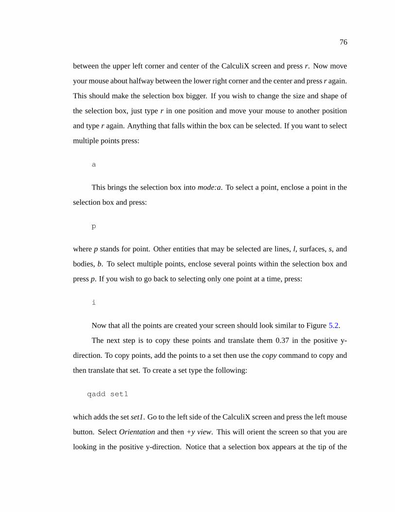
76
between the upper left corner and center of the CalculiX screen and press r. Now move
your mouse about halfway between the lower right corner and the center and press r again.
This should make the selection box bigger. If you wish to change the size and shape of
the selection box, just type r in one position and move your mouse to another position
and type r again. Anything that falls within the box can be selected. If you want to select
multiple points press:
a
This brings the selection box into mode:a. To select a point, enclose a point in the
selection box and press:
p
where p stands for point. Other entities that may be selected are lines, l, surfaces, s, and
bodies, b. To select multiple points, enclose several points within the selection box and
press p. If you wish to go back to selecting only one point at a time, press:
i
Now that all the points are created your screen should look similar to Figure 5.2.
The next step is to copy these points and translate them 0.37 in the positive y-
direction. To copy points, add the points to a set then use the copy command to copy and
then translate that set. To create a set type the following:
qadd set1
which adds the set set1. Go to the left side of the CalculiX screen and press the left mouse
button. Select Orientation and then +y view. This will orient the screen so that you are
looking in the positive y-direction. Notice that a selection box appears at the tip of the
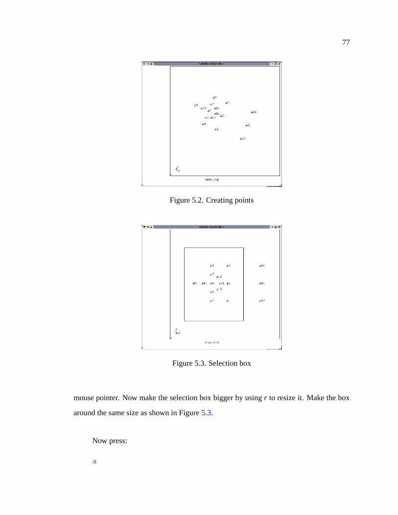
77
Figure 5.2. Creating points
Figure 5.3. Selection box
mouse pointer. Now make the selection box bigger by using r to resize it. Make the box
around the same size as shown in Figure 5.3.
Now press:
a
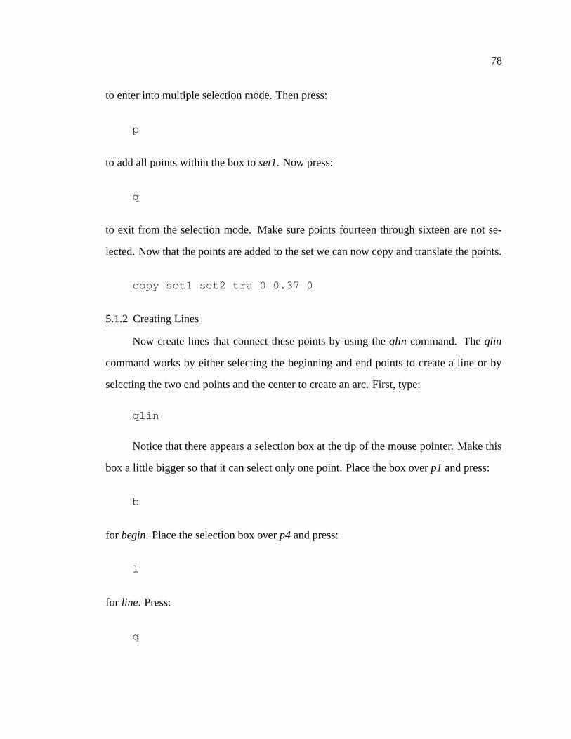
78
to enter into multiple selection mode. Then press:
p
to add all points within the box to set1. Now press:
q
to exit from the selection mode. Make sure points fourteen through sixteen are not se-
lected. Now that the points are added to the set we can now copy and translate the points.
copy set1 set2 tra 0 0.37 0
5.1.2 Creating Lines
Now create lines that connect these points by using the qlin command. The qlin
command works by either selecting the beginning and end points to create a line or by
selecting the two end points and the center to create an arc. First, type:
qlin
Notice that there appears a selection box at the tip of the mouse pointer. Make this
box a little bigger so that it can select only one point. Place the box over p1 and press:
b
for begin. Place the selection box over p4 and press:
l
for line. Press:
q
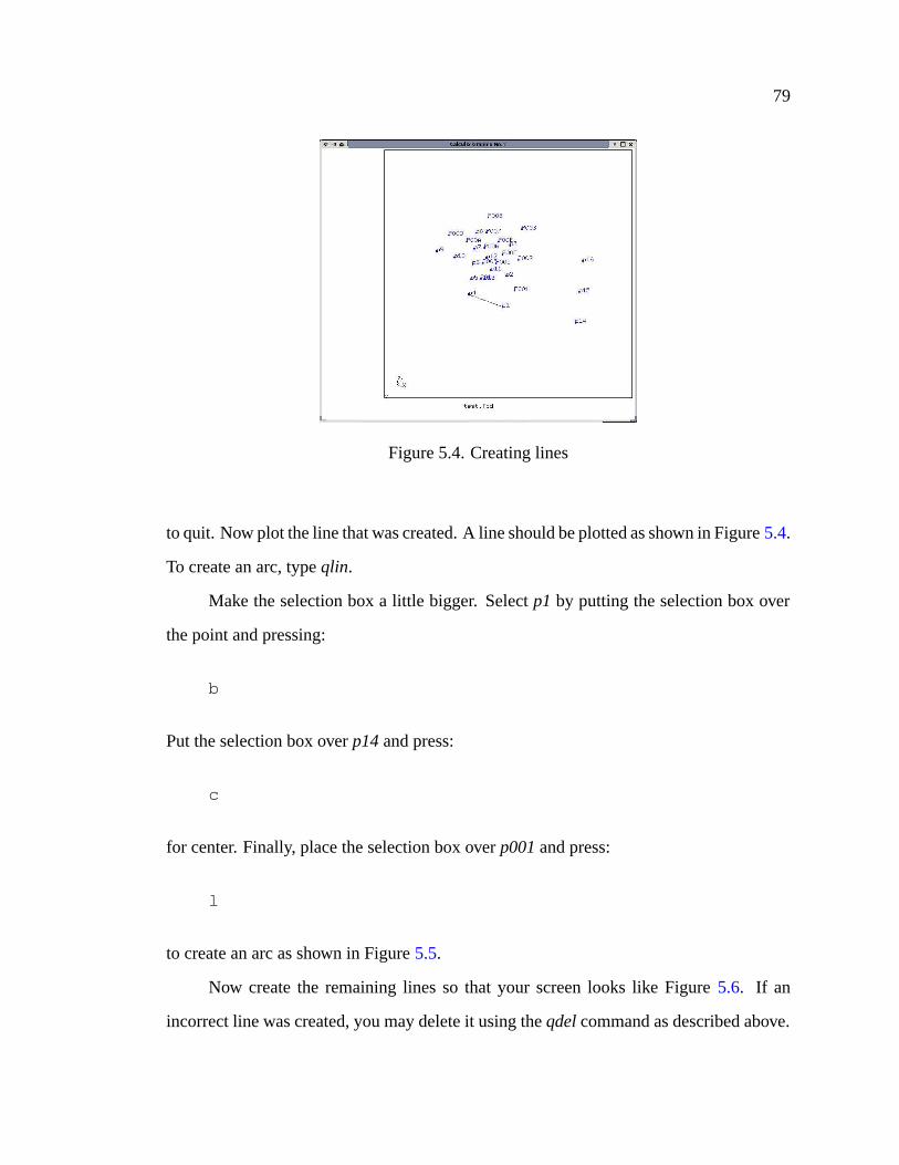
79
Figure 5.4. Creating lines
to quit. Now plot the line that was created. A line should be plotted as shown in Figure 5.4.
To create an arc, type qlin.
Make the selection box a little bigger. Select p1 by putting the selection box over
the point and pressing:
b
Put the selection box over p14 and press:
c
for center. Finally, place the selection box over p001 and press:
l
to create an arc as shown in Figure 5.5.
Now create the remaining lines so that your screen looks like Figure 5.6. If an
incorrect line was created, you may delete it using the qdel command as described above.
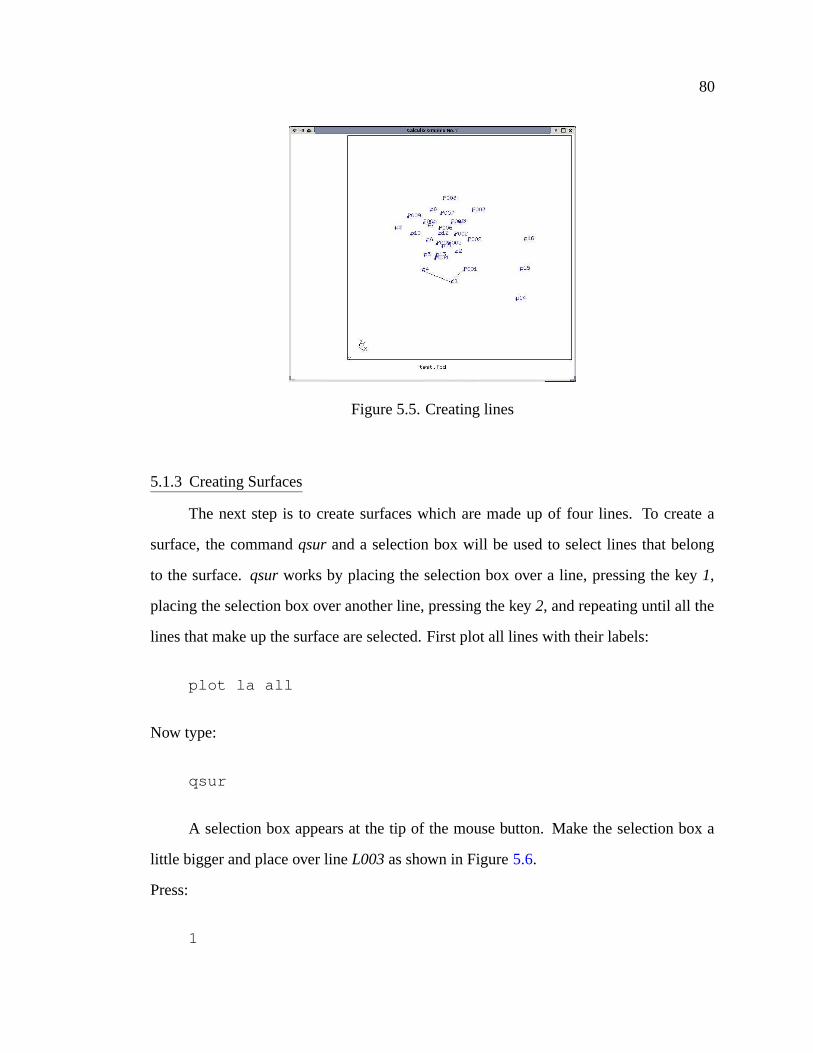
80
Figure 5.5. Creating lines
5.1.3 Creating Surfaces
The next step is to create surfaces which are made up of four lines. To create a
surface, the command qsur and a selection box will be used to select lines that belong
to the surface. qsur works by placing the selection box over a line, pressing the key 1,
placing the selection box over another line, pressing the key 2, and repeating until all the
lines that make up the surface are selected. First plot all lines with their labels:
plot la all
Now type:
qsur
A selection box appears at the tip of the mouse button. Make the selection box a
little bigger and place over line L003 as shown in Figure 5.6.
Press:
1

81
Figure 5.6. Creating surfaces
and the line will turn red. Put the selection box over line L005 and press:
2
Now put the selection box over line L00K and press:
3
Finally, put the selection box over line L004 and press:
4
Now press:
g
to generate the surface. Press:
q
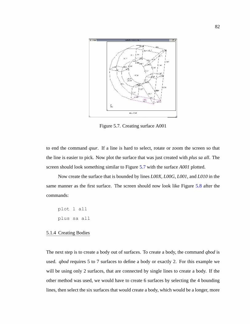
82
Figure 5.7. Creating surface A001
to end the command qsur. If a line is hard to select, rotate or zoom the screen so that
the line is easier to pick. Now plot the surface that was just created with plus sa all. The
screen should look something similar to Figure 5.7 with the surface A001 plotted.
Now create the surface that is bounded by lines L00X, L00G, L001, and L010 in the
same manner as the first surface. The screen should now look like Figure 5.8 after the
commands:
plot l all
plus sa all
5.1.4 Creating Bodies
The next step is to create a body out of surfaces. To create a body, the command qbod is
used. qbod requires 5 to 7 surfaces to define a body or exactly 2. For this example we
will be using only 2 surfaces, that are connected by single lines to create a body. If the
other method was used, we would have to create 6 surfaces by selecting the 4 bounding
lines, then select the six surfaces that would create a body, which would be a longer, more
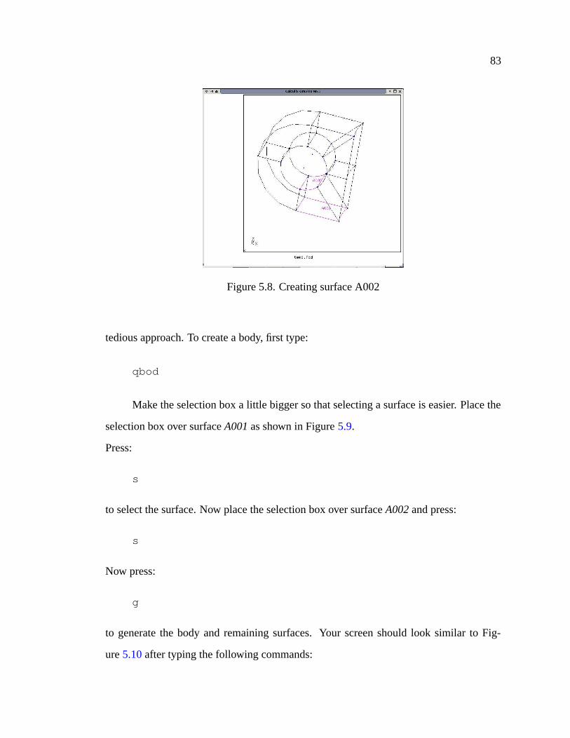
83
Figure 5.8. Creating surface A002
tedious approach. To create a body, first type:
qbod
Make the selection box a little bigger so that selecting a surface is easier. Place the
selection box over surface A001 as shown in Figure 5.9.
Press:
s
to select the surface. Now place the selection box over surface A002 and press:
s
Now press:
g
to generate the body and remaining surfaces. Your screen should look similar to Fig-
ure 5.10 after typing the following commands:
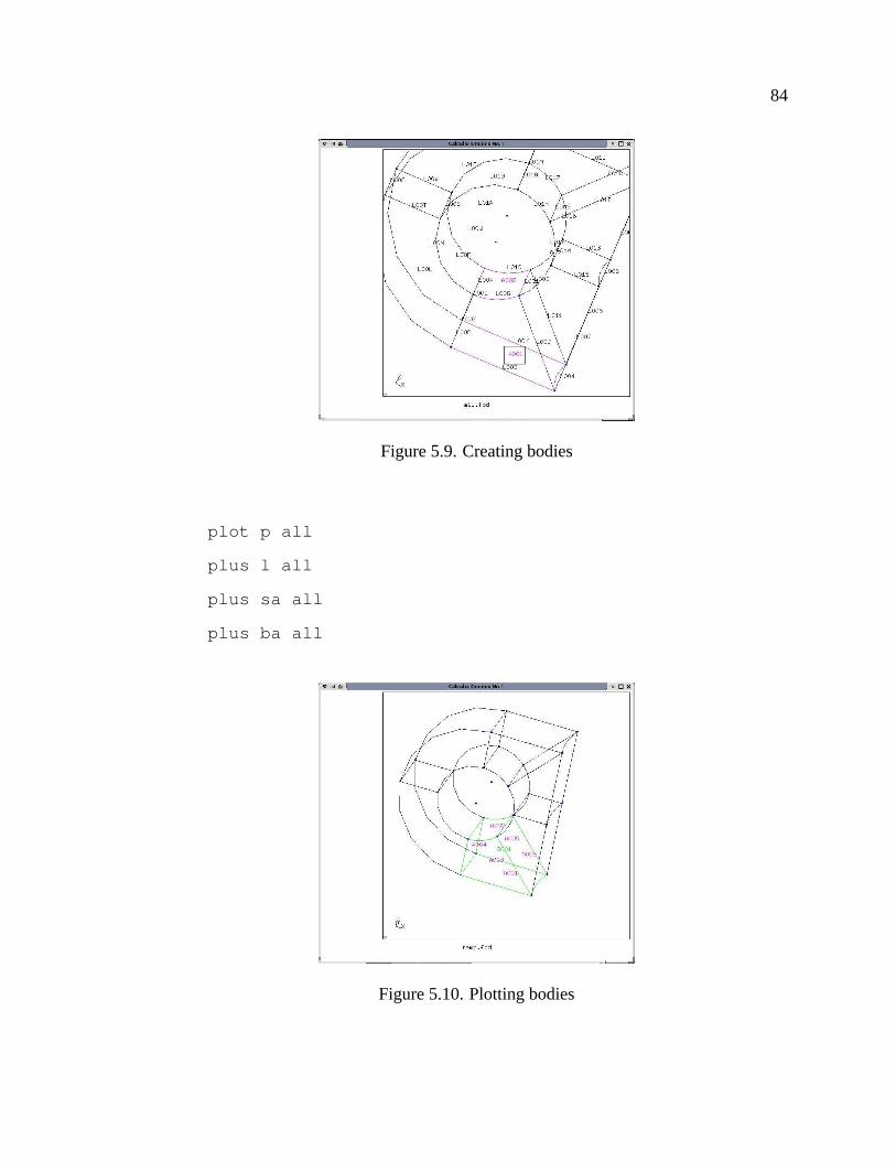
84
Figure 5.9. Creating bodies
plot p all
plus l all
plus sa all
plus ba all
Figure 5.10. Plotting bodies
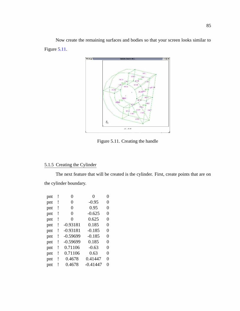
85
Now create the remaining surfaces and bodies so that your screen looks similar to
Figure 5.11.
Figure 5.11. Creating the handle
5.1.5 Creating the Cylinder
The next feature that will be created is the cylinder. First, create points that are on
the cylinder boundary.
pnt ! 0 0 0pnt ! 0 -0.95 0pnt ! 0 0.95 0pnt ! 0 -0.625 0pnt ! 0 0.625 0pnt ! -0.93181 0.185 0pnt ! -0.93181 -0.185 0pnt ! -0.59699 -0.185 0pnt ! -0.59699 0.185 0pnt ! 0.71106 -0.63 0pnt ! 0.71106 0.63 0pnt ! 0.4678 0.41447 0pnt ! 0.4678 -0.41447 0
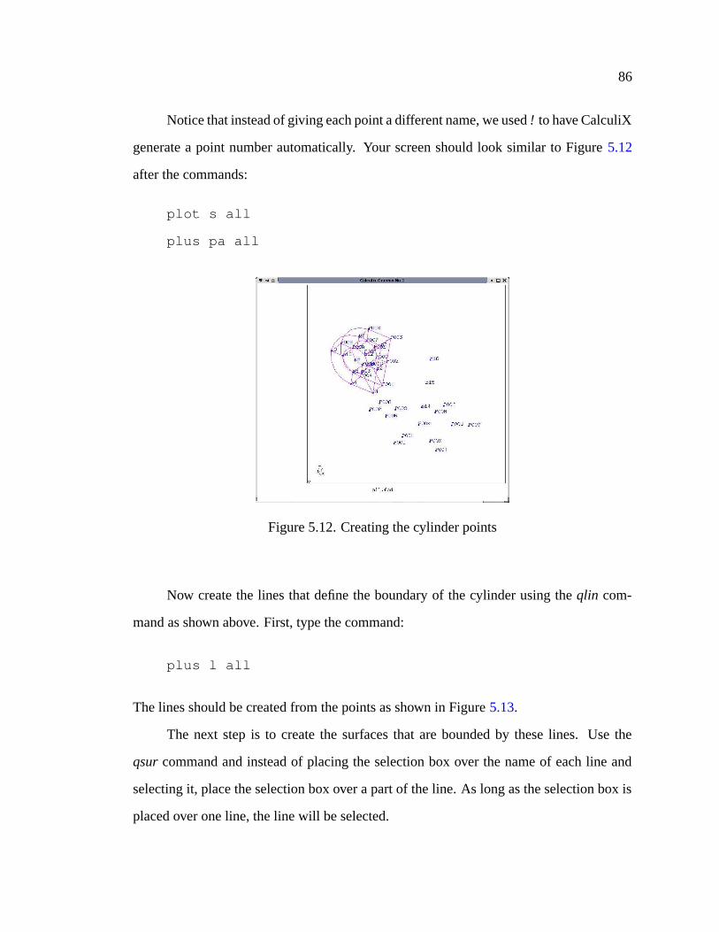
86
Notice that instead of giving each point a different name, we used ! to have CalculiX
generate a point number automatically. Your screen should look similar to Figure 5.12
after the commands:
plot s all
plus pa all
Figure 5.12. Creating the cylinder points
Now create the lines that define the boundary of the cylinder using the qlin com-
mand as shown above. First, type the command:
plus l all
The lines should be created from the points as shown in Figure 5.13.
The next step is to create the surfaces that are bounded by these lines. Use the
qsur command and instead of placing the selection box over the name of each line and
selecting it, place the selection box over a part of the line. As long as the selection box is
placed over one line, the line will be selected.

87
Figure 5.13. Creating the cylinder lines
Make the selection box a little bigger and press numbers one through four for each
line that the selection box is over. After the four lines are selected press g. This will
generate the surface. After the surfaces have been generated, your screen should look
similar to Figure 5.14 after the command:
plus sa all
The next step is to create the bodies that define the cylinder. First, add all surfaces
belonging to the cylinder to a set called cylinder1. The name of the surfaces that appears
in Figure 5.15 may be different from the names on your screen. This does not matter, just
select the same surfaces.
Type the command:
qadd cylinder1
A little square appears around the tip of the mouse pointer. To increase the size of
the selection box, with your mouse pointer in the main screen, press r, move the mouse
pointer a little lower and to the right, and press r again. Move your mouse such that the
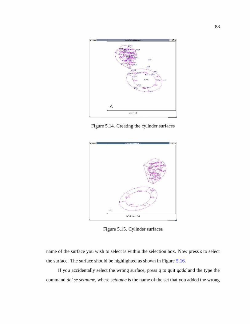
88
Figure 5.14. Creating the cylinder surfaces
Figure 5.15. Cylinder surfaces
name of the surface you wish to select is within the selection box. Now press s to select
the surface. The surface should be highlighted as shown in Figure 5.16.
If you accidentally select the wrong surface, press q to quit qadd and the type the
command del se setname, where setname is the name of the set that you added the wrong
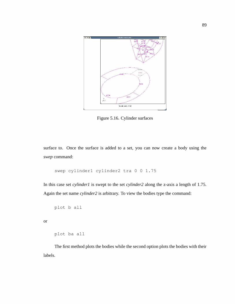
89
Figure 5.16. Cylinder surfaces
surface to. Once the surface is added to a set, you can now create a body using the
swep command:
swep cylinder1 cylinder2 tra 0 0 1.75
In this case set cylinder1 is swept to the set cylinder2 along the z-axis a length of 1.75.
Again the set name cylinder2 is arbitrary. To view the bodies type the command:
plot b all
or
plot ba all
The first method plots the bodies while the second option plots the bodies with their
labels.
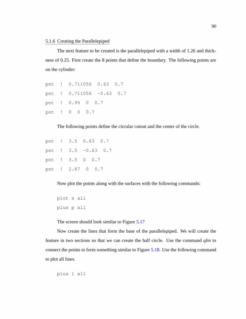
90
5.1.6 Creating the Parallelepiped
The next feature to be created is the parallelepiped with a width of 1.26 and thick-
ness of 0.25. First create the 8 points that define the boundary. The following points are
on the cylinder:
pnt ! 0.711056 0.63 0.7
pnt ! 0.711056 -0.63 0.7
pnt ! 0.95 0 0.7
pnt ! 0 0 0.7
The following points define the circular cutout and the center of the circle.
pnt ! 3.5 0.63 0.7
pnt ! 3.5 -0.63 0.7
pnt ! 3.5 0 0.7
pnt ! 2.87 0 0.7
Now plot the points along with the surfaces with the following commands:
plot s all
plus p all
The screen should look similar to Figure 5.17
Now create the lines that form the base of the parallelepiped. We will create the
feature in two sections so that we can create the half circle. Use the command qlin to
connect the points to form something similar to Figure 5.18. Use the following command
to plot all lines.
plus l all

91
Figure 5.17. Creating points for parallelepiped
Figure 5.18. Creating lines for parallelepiped
Now create the bottom two surfaces. Use the qsur command and select four lines that
belong to one section and generate that surface. Repeat this procedure for the remaining
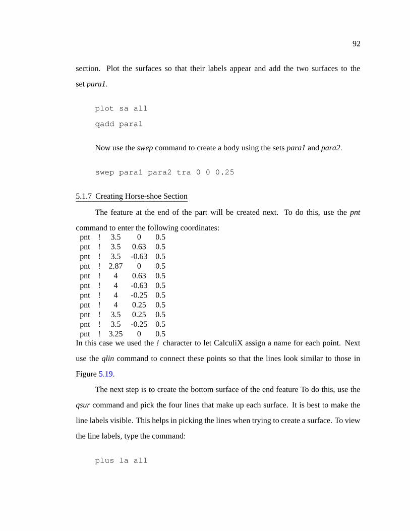
92
section. Plot the surfaces so that their labels appear and add the two surfaces to the
set para1.
plot sa all
qadd para1
Now use the swep command to create a body using the sets para1 and para2.
swep para1 para2 tra 0 0 0.25
5.1.7 Creating Horse-shoe Section
The feature at the end of the part will be created next. To do this, use the pnt
command to enter the following coordinates:pnt ! 3.5 0 0.5pnt ! 3.5 0.63 0.5pnt ! 3.5 -0.63 0.5pnt ! 2.87 0 0.5pnt ! 4 0.63 0.5pnt ! 4 -0.63 0.5pnt ! 4 -0.25 0.5pnt ! 4 0.25 0.5pnt ! 3.5 0.25 0.5pnt ! 3.5 -0.25 0.5pnt ! 3.25 0 0.5
In this case we used the ! character to let CalculiX assign a name for each point. Next
use the qlin command to connect these points so that the lines look similar to those in
Figure 5.19.
The next step is to create the bottom surface of the end feature To do this, use the
qsur command and pick the four lines that make up each surface. It is best to make the
line labels visible. This helps in picking the lines when trying to create a surface. To view
the line labels, type the command:
plus la all
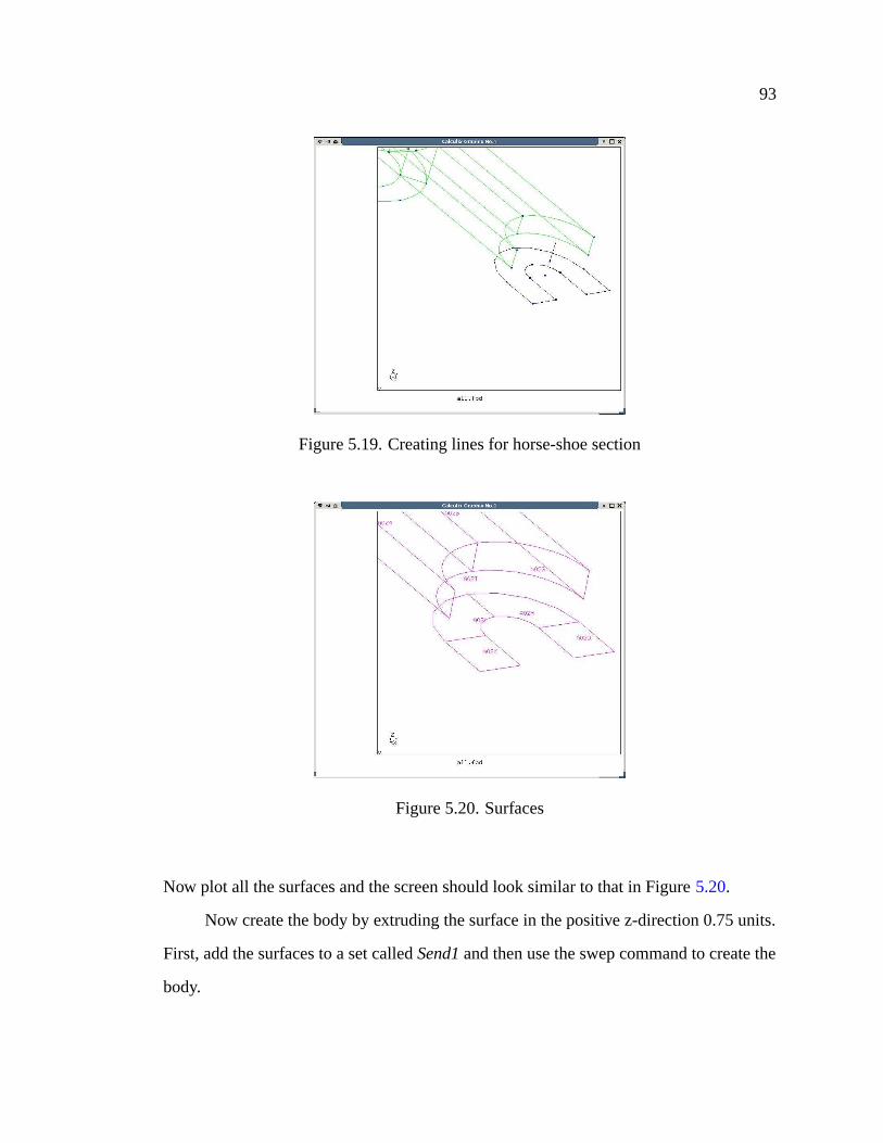
93
Figure 5.19. Creating lines for horse-shoe section
Figure 5.20. Surfaces
Now plot all the surfaces and the screen should look similar to that in Figure 5.20.
Now create the body by extruding the surface in the positive z-direction 0.75 units.
First, add the surfaces to a set called Send1 and then use the swep command to create the
body.
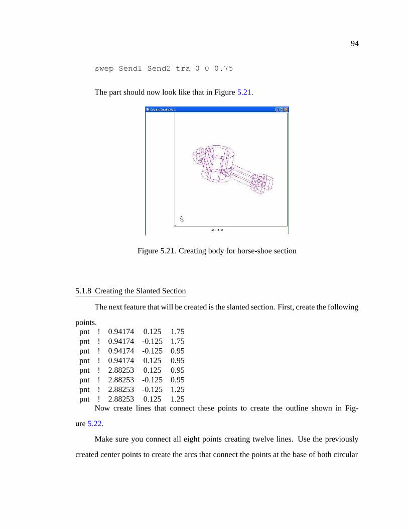
94
swep Send1 Send2 tra 0 0 0.75
The part should now look like that in Figure 5.21.
Figure 5.21. Creating body for horse-shoe section
5.1.8 Creating the Slanted Section
The next feature that will be created is the slanted section. First, create the following
points.pnt ! 0.94174 0.125 1.75pnt ! 0.94174 -0.125 1.75pnt ! 0.94174 -0.125 0.95pnt ! 0.94174 0.125 0.95pnt ! 2.88253 0.125 0.95pnt ! 2.88253 -0.125 0.95pnt ! 2.88253 -0.125 1.25pnt ! 2.88253 0.125 1.25
Now create lines that connect these points to create the outline shown in Fig-
ure 5.22.
Make sure you connect all eight points creating twelve lines. Use the previously
created center points to create the arcs that connect the points at the base of both circular
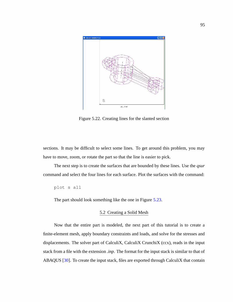
95
Figure 5.22. Creating lines for the slanted section
sections. It may be difficult to select some lines. To get around this problem, you may
have to move, zoom, or rotate the part so that the line is easier to pick.
The next step is to create the surfaces that are bounded by these lines. Use the qsur
command and select the four lines for each surface. Plot the surfaces with the command:
plot s all
The part should look something like the one in Figure 5.23.
5.2 Creating a Solid Mesh
Now that the entire part is modeled, the next part of this tutorial is to create a
finite-element mesh, apply boundary constraints and loads, and solve for the stresses and
displacements. The solver part of CalculiX, CalculiX CrunchiX (ccx), reads in the input
stack from a file with the extension .inp. The format for the input stack is similar to that of
ABAQUS [30]. To create the input stack, files are exported through CalculiX that contain
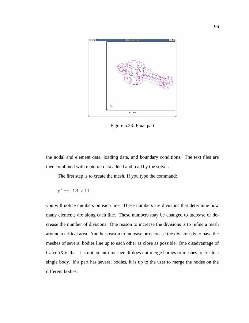
96
Figure 5.23. Final part
the nodal and element data, loading data, and boundary conditions. The text files are
then combined with material data added and read by the solver.
The first step is to create the mesh. If you type the command:
plot ld all
you will notice numbers on each line. These numbers are divisions that determine how
many elements are along each line. These numbers may be changed to increase or de-
crease the number of divisions. One reason to increase the divisions is to refine a mesh
around a critical area. Another reason to increase or decrease the divisions is to have the
meshes of several bodies line up to each other as close as possible. One disadvantage of
CalculiX is that it is not an auto-mesher. It does not merge bodies or meshes to create a
single body. If a part has several bodies, it is up to the user to merge the nodes on the
different bodies.
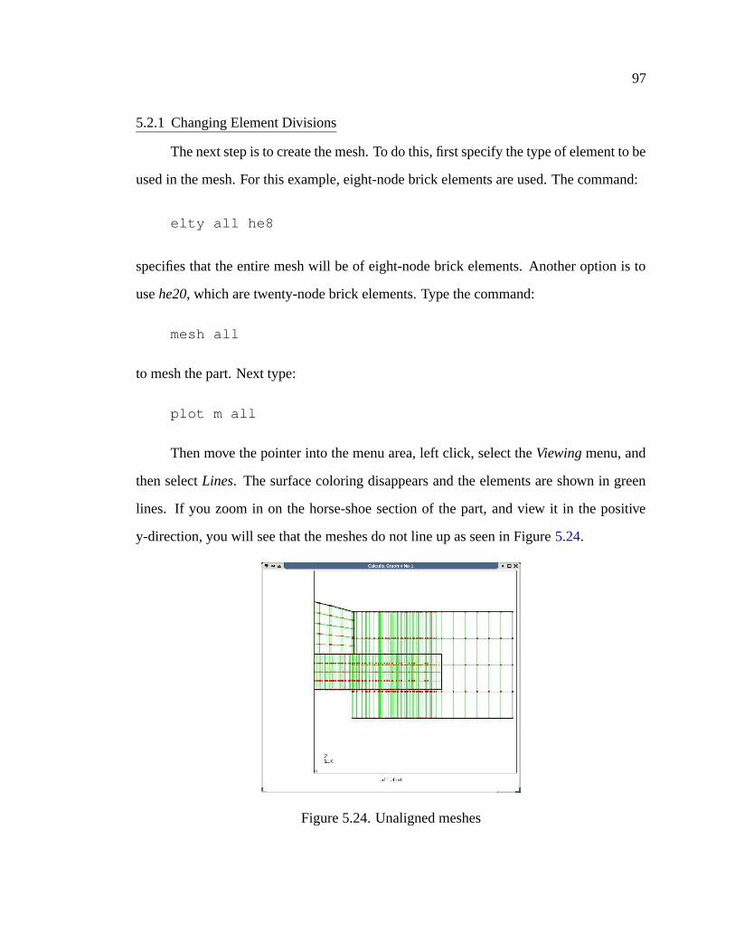
97
5.2.1 Changing Element Divisions
The next step is to create the mesh. To do this, first specify the type of element to be
used in the mesh. For this example, eight-node brick elements are used. The command:
elty all he8
specifies that the entire mesh will be of eight-node brick elements. Another option is to
use he20, which are twenty-node brick elements. Type the command:
mesh all
to mesh the part. Next type:
plot m all
Then move the pointer into the menu area, left click, select the Viewing menu, and
then select Lines. The surface coloring disappears and the elements are shown in green
lines. If you zoom in on the horse-shoe section of the part, and view it in the positive
y-direction, you will see that the meshes do not line up as seen in Figure 5.24.
Figure 5.24. Unaligned meshes
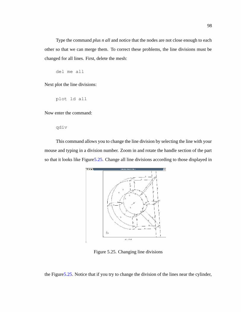
98
Type the command plus n all and notice that the nodes are not close enough to each
other so that we can merge them. To correct these problems, the line divisions must be
changed for all lines. First, delete the mesh:
del me all
Next plot the line divisions:
plot ld all
Now enter the command:
qdiv
This command allows you to change the line division by selecting the line with your
mouse and typing in a division number. Zoom in and rotate the handle section of the part
so that it looks like Figure5.25. Change all line divisions according to those displayed in
Figure 5.25. Changing line divisions
the Figure5.25. Notice that if you try to change the division of the lines near the cylinder,
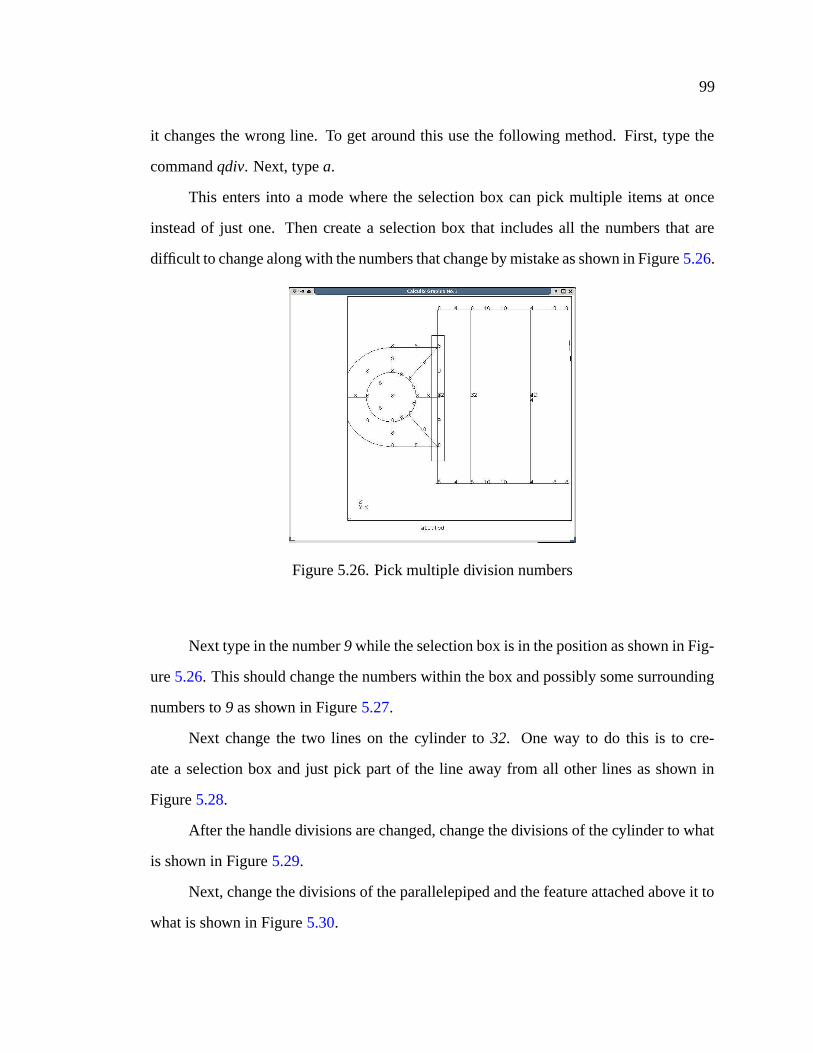
99
it changes the wrong line. To get around this use the following method. First, type the
command qdiv. Next, type a.
This enters into a mode where the selection box can pick multiple items at once
instead of just one. Then create a selection box that includes all the numbers that are
difficult to change along with the numbers that change by mistake as shown in Figure 5.26.
Figure 5.26. Pick multiple division numbers
Next type in the number 9 while the selection box is in the position as shown in Fig-
ure 5.26. This should change the numbers within the box and possibly some surrounding
numbers to 9 as shown in Figure 5.27.
Next change the two lines on the cylinder to 32. One way to do this is to cre-
ate a selection box and just pick part of the line away from all other lines as shown in
Figure 5.28.
After the handle divisions are changed, change the divisions of the cylinder to what
is shown in Figure 5.29.
Next, change the divisions of the parallelepiped and the feature attached above it to
what is shown in Figure 5.30.
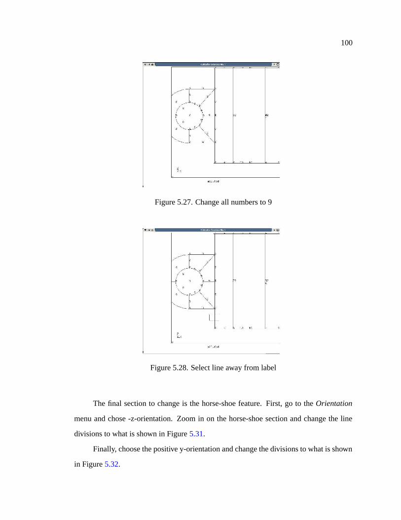
100
Figure 5.27. Change all numbers to 9
Figure 5.28. Select line away from label
The final section to change is the horse-shoe feature. First, go to the Orientation
menu and chose -z-orientation. Zoom in on the horse-shoe section and change the line
divisions to what is shown in Figure 5.31.
Finally, choose the positive y-orientation and change the divisions to what is shown
in Figure 5.32.
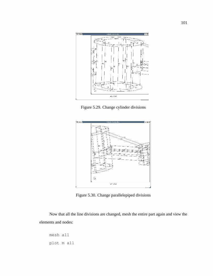
101
Figure 5.29. Change cylinder divisions
Figure 5.30. Change parallelepiped divisions
Now that all the line divisions are changed, mesh the entire part again and view the
elements and nodes:
mesh all
plot m all
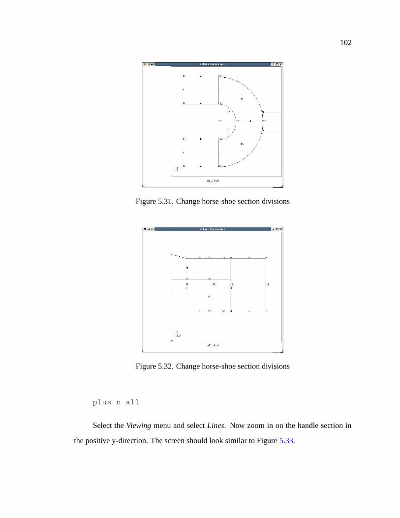
102
Figure 5.31. Change horse-shoe section divisions
Figure 5.32. Change horse-shoe section divisions
plus n all
Select the Viewing menu and select Lines. Now zoom in on the handle section in
the positive y-direction. The screen should look similar to Figure 5.33.
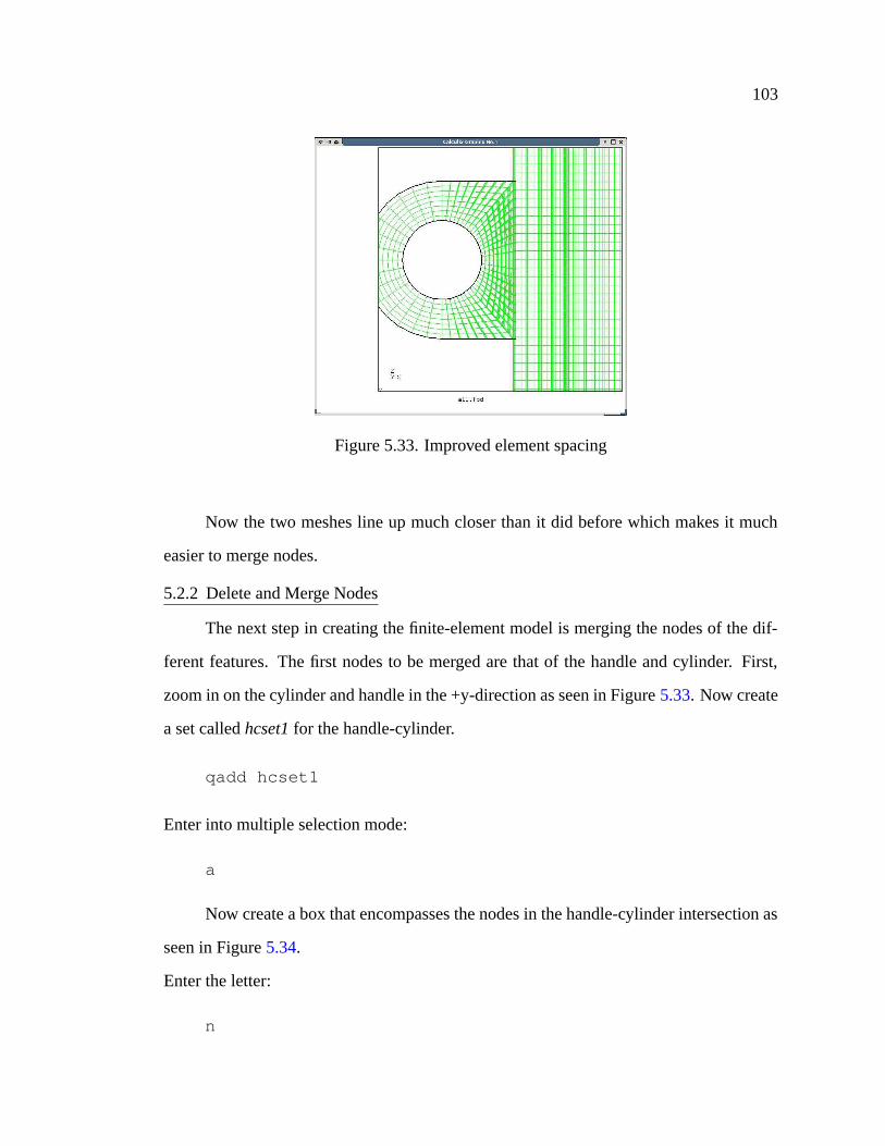
103
Figure 5.33. Improved element spacing
Now the two meshes line up much closer than it did before which makes it much
easier to merge nodes.
5.2.2 Delete and Merge Nodes
The next step in creating the finite-element model is merging the nodes of the dif-
ferent features. The first nodes to be merged are that of the handle and cylinder. First,
zoom in on the cylinder and handle in the +y-direction as seen in Figure 5.33. Now create
a set called hcset1 for the handle-cylinder.
qadd hcset1
Enter into multiple selection mode:
a
Now create a box that encompasses the nodes in the handle-cylinder intersection as
seen in Figure 5.34.
Enter the letter:
n
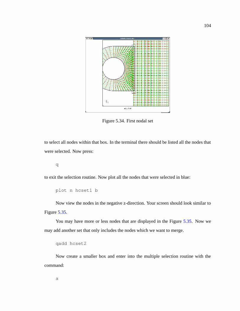
104
Figure 5.34. First nodal set
to select all nodes within that box. In the terminal there should be listed all the nodes that
were selected. Now press:
q
to exit the selection routine. Now plot all the nodes that were selected in blue:
plot n hcset1 b
Now view the nodes in the negative z-direction. Your screen should look similar to
Figure 5.35.
You may have more or less nodes that are displayed in the Figure 5.35. Now we
may add another set that only includes the nodes which we want to merge.
qadd hcset2
Now create a smaller box and enter into the multiple selection routine with the
command:
a
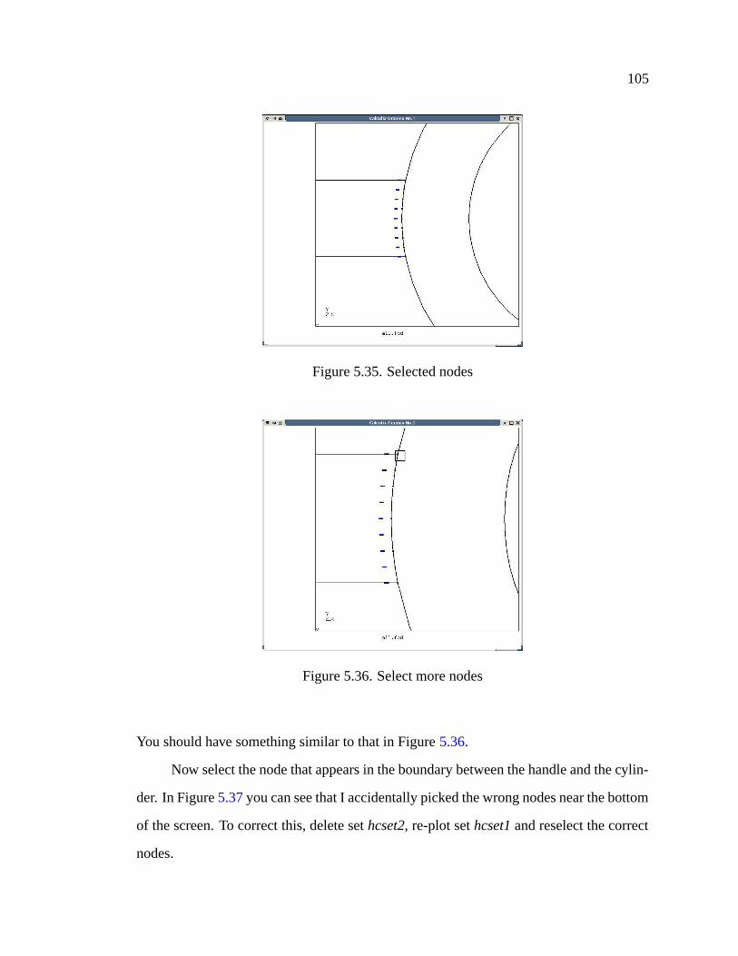
105
Figure 5.35. Selected nodes
Figure 5.36. Select more nodes
You should have something similar to that in Figure 5.36.
Now select the node that appears in the boundary between the handle and the cylin-
der. In Figure 5.37 you can see that I accidentally picked the wrong nodes near the bottom
of the screen. To correct this, delete set hcset2, re-plot set hcset1 and reselect the correct
nodes.
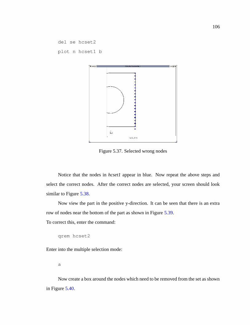
106
del se hcset2
plot n hcset1 b
Figure 5.37. Selected wrong nodes
Notice that the nodes in hcset1 appear in blue. Now repeat the above steps and
select the correct nodes. After the correct nodes are selected, your screen should look
similar to Figure 5.38.
Now view the part in the positive y-direction. It can be seen that there is an extra
row of nodes near the bottom of the part as shown in Figure 5.39.
To correct this, enter the command:
qrem hcset2
Enter into the multiple selection mode:
a
Now create a box around the nodes which need to be removed from the set as shown
in Figure 5.40.
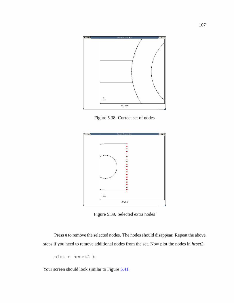
107
Figure 5.38. Correct set of nodes
Figure 5.39. Selected extra nodes
Press n to remove the selected nodes. The nodes should disappear. Repeat the above
steps if you need to remove additional nodes from the set. Now plot the nodes in hcset2.
plot n hcset2 b
Your screen should look similar to Figure 5.41.
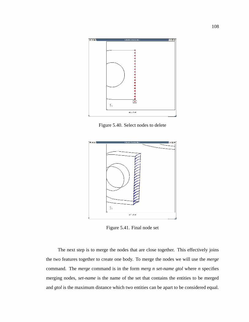
108
Figure 5.40. Select nodes to delete
Figure 5.41. Final node set
The next step is to merge the nodes that are close together. This effectively joins
the two features together to create one body. To merge the nodes we will use the merge
command. The merge command is in the form merg n set-name gtol where n specifies
merging nodes, set-name is the name of the set that contains the entities to be merged
and gtol is the maximum distance which two entities can be apart to be considered equal.
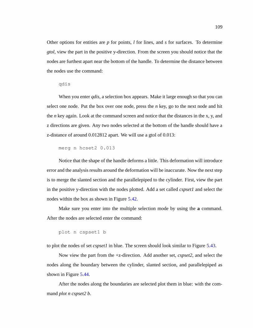
109
Other options for entities are p for points, l for lines, and s for surfaces. To determine
gtol, view the part in the positive y-direction. From the screen you should notice that the
nodes are furthest apart near the bottom of the handle. To determine the distance between
the nodes use the command:
qdis
When you enter qdis, a selection box appears. Make it large enough so that you can
select one node. Put the box over one node, press the n key, go to the next node and hit
the n key again. Look at the command screen and notice that the distances in the x, y, and
z directions are given. Any two nodes selected at the bottom of the handle should have a
z-distance of around 0.012812 apart. We will use a gtol of 0.013:
merg n hcset2 0.013
Notice that the shape of the handle deforms a little. This deformation will introduce
error and the analysis results around the deformation will be inaccurate. Now the next step
is to merge the slanted section and the parallelepiped to the cylinder. First, view the part
in the positive y-direction with the nodes plotted. Add a set called cspset1 and select the
nodes within the box as shown in Figure 5.42.
Make sure you enter into the multiple selection mode by using the a command.
After the nodes are selected enter the command:
plot n cspset1 b
to plot the nodes of set cspset1 in blue. The screen should look similar to Figure 5.43.
Now view the part from the +z-direction. Add another set, cspset2, and select the
nodes along the boundary between the cylinder, slanted section, and parallelepiped as
shown in Figure 5.44.
After the nodes along the boundaries are selected plot them in blue: with the com-
mand plot n cspset2 b.
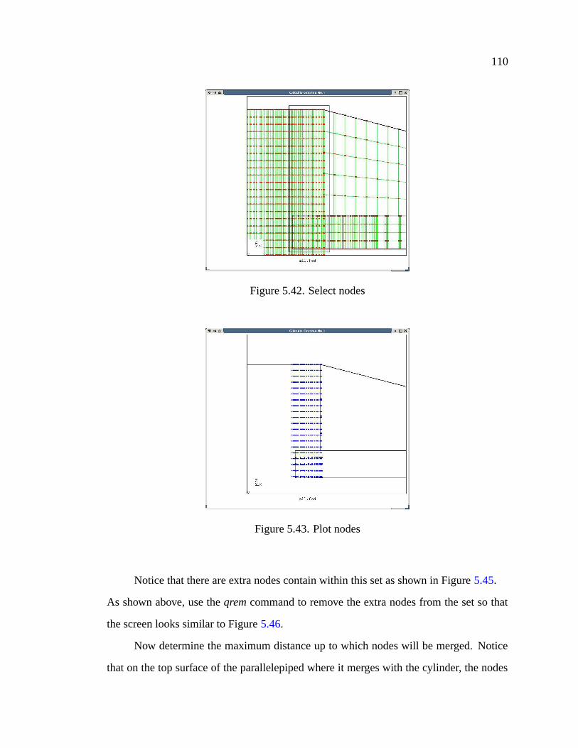
110
Figure 5.42. Select nodes
Figure 5.43. Plot nodes
Notice that there are extra nodes contain within this set as shown in Figure 5.45.
As shown above, use the qrem command to remove the extra nodes from the set so that
the screen looks similar to Figure 5.46.
Now determine the maximum distance up to which nodes will be merged. Notice
that on the top surface of the parallelepiped where it merges with the cylinder, the nodes
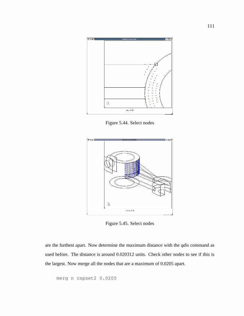
111
Figure 5.44. Select nodes
Figure 5.45. Select nodes
are the furthest apart. Now determine the maximum distance with the qdis command as
used before. The distance is around 0.020312 units. Check other nodes to see if this is
the largest. Now merge all the nodes that are a maximum of 0.0205 apart.
merg n cspset2 0.0205
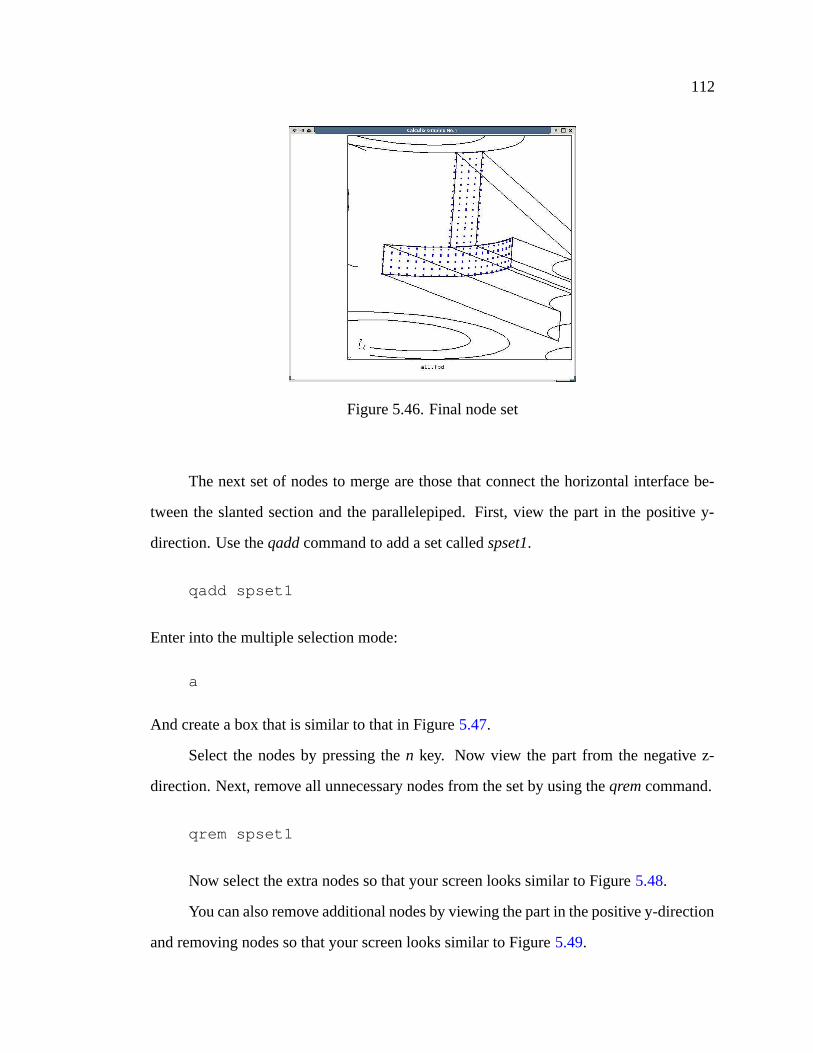
112
Figure 5.46. Final node set
The next set of nodes to merge are those that connect the horizontal interface be-
tween the slanted section and the parallelepiped. First, view the part in the positive y-
direction. Use the qadd command to add a set called spset1.
qadd spset1
Enter into the multiple selection mode:
a
And create a box that is similar to that in Figure 5.47.
Select the nodes by pressing the n key. Now view the part from the negative z-
direction. Next, remove all unnecessary nodes from the set by using the qrem command.
qrem spset1
Now select the extra nodes so that your screen looks similar to Figure 5.48.
You can also remove additional nodes by viewing the part in the positive y-direction
and removing nodes so that your screen looks similar to Figure 5.49.
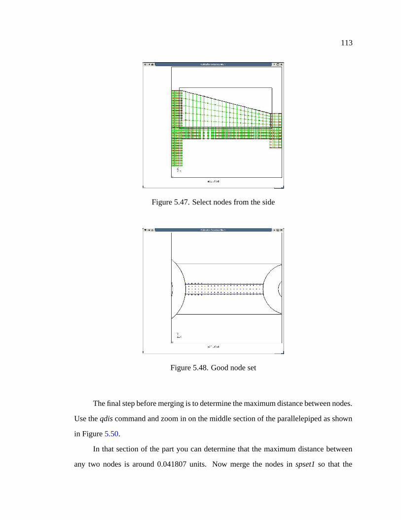
113
Figure 5.47. Select nodes from the side
Figure 5.48. Good node set
The final step before merging is to determine the maximum distance between nodes.
Use the qdis command and zoom in on the middle section of the parallelepiped as shown
in Figure 5.50.
In that section of the part you can determine that the maximum distance between
any two nodes is around 0.041807 units. Now merge the nodes in spset1 so that the
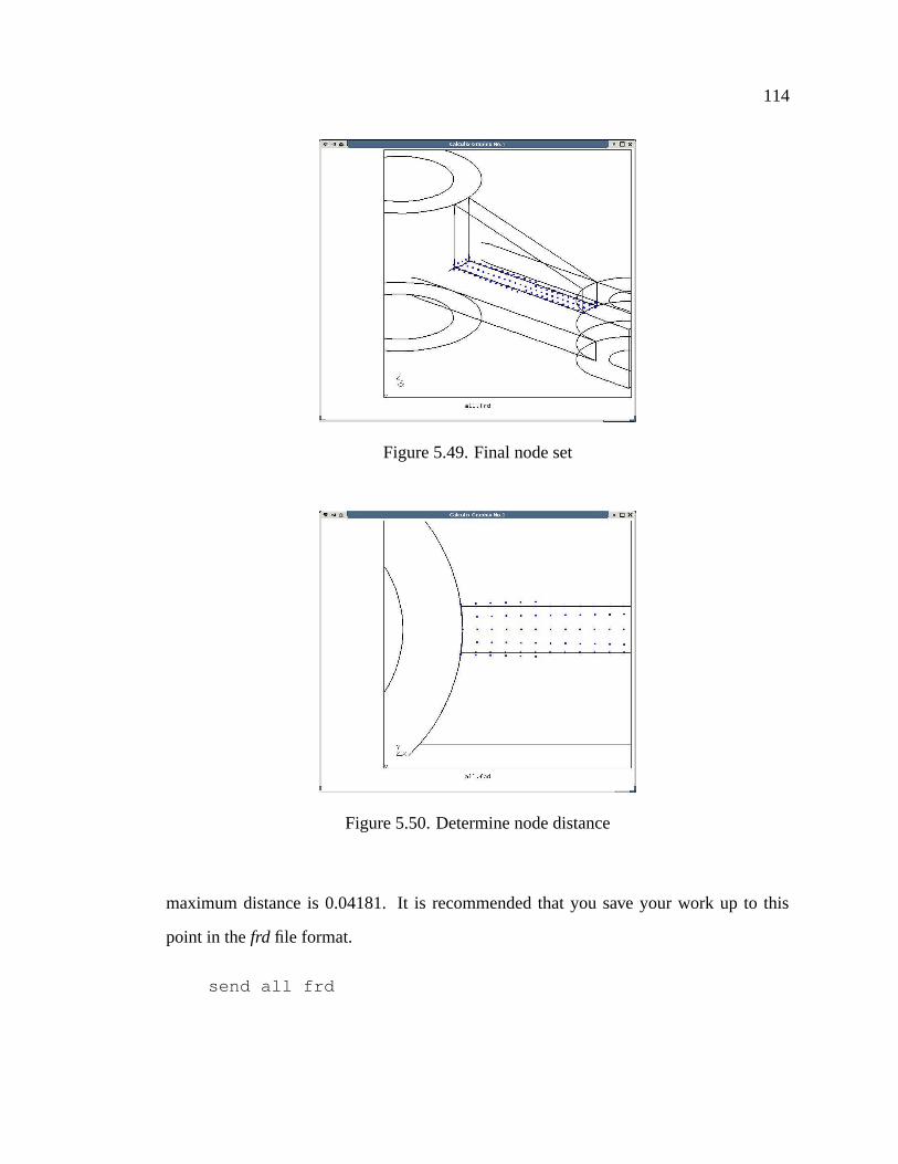
114
Figure 5.49. Final node set
Figure 5.50. Determine node distance
maximum distance is 0.04181. It is recommended that you save your work up to this
point in the frd file format.
send all frd
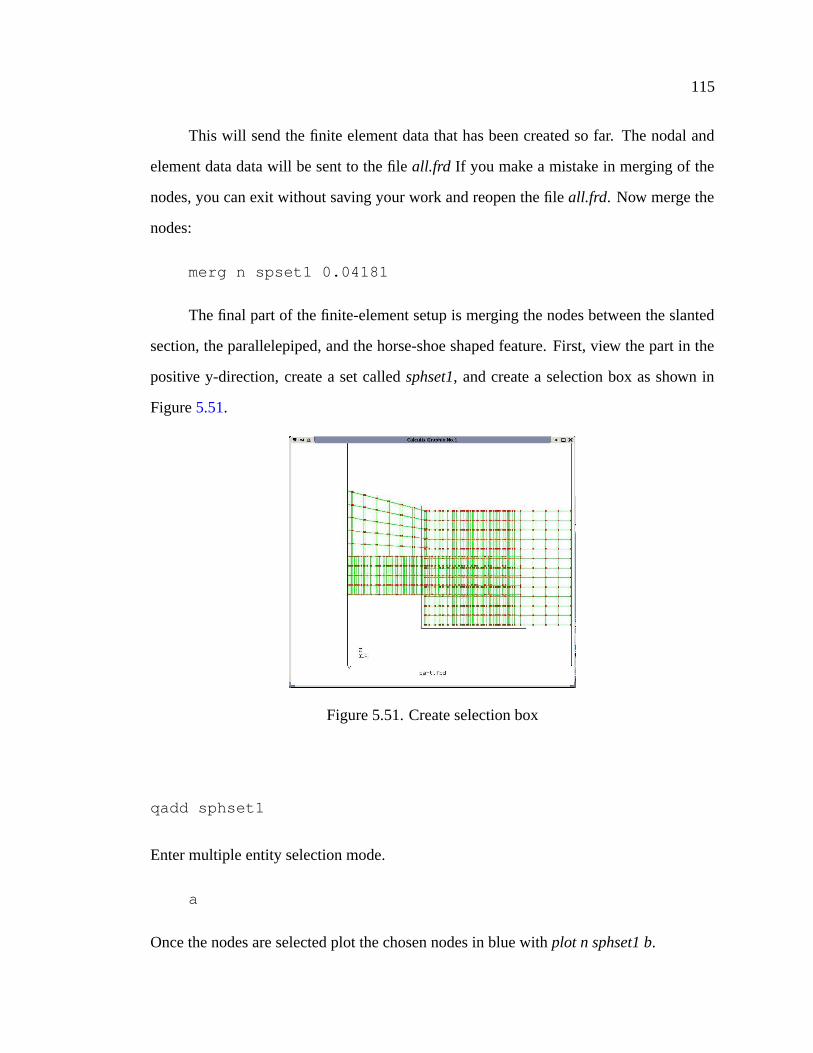
115
This will send the finite element data that has been created so far. The nodal and
element data data will be sent to the file all.frd If you make a mistake in merging of the
nodes, you can exit without saving your work and reopen the file all.frd. Now merge the
nodes:
merg n spset1 0.04181
The final part of the finite-element setup is merging the nodes between the slanted
section, the parallelepiped, and the horse-shoe shaped feature. First, view the part in the
positive y-direction, create a set called sphset1, and create a selection box as shown in
Figure 5.51.
Figure 5.51. Create selection box
qadd sphset1
Enter multiple entity selection mode.
a
Once the nodes are selected plot the chosen nodes in blue with plot n sphset1 b.
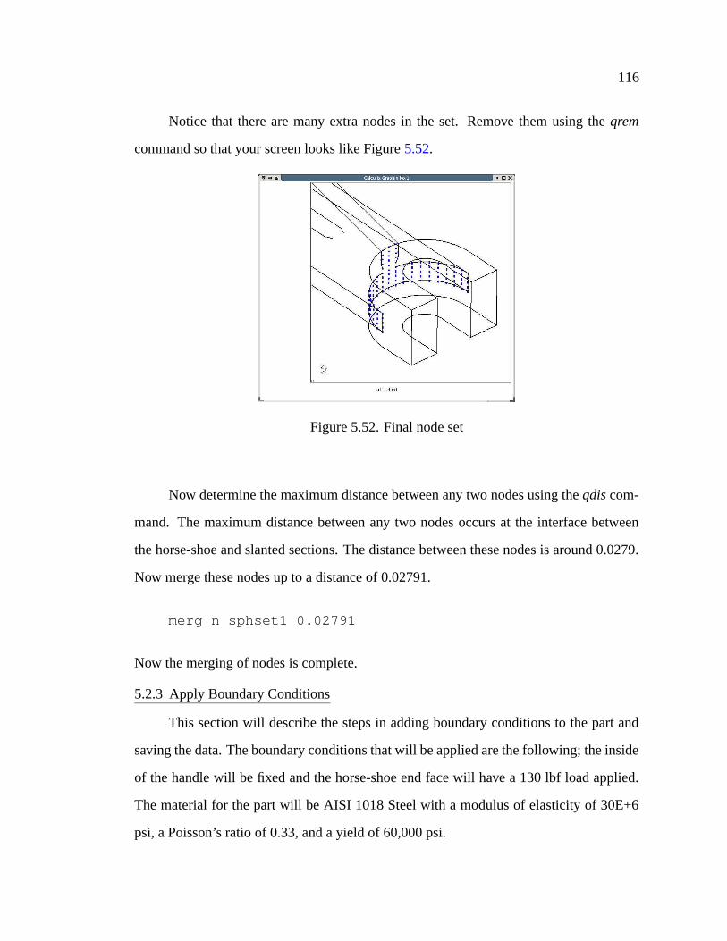
116
Notice that there are many extra nodes in the set. Remove them using the qrem
command so that your screen looks like Figure 5.52.
Figure 5.52. Final node set
Now determine the maximum distance between any two nodes using the qdis com-
mand. The maximum distance between any two nodes occurs at the interface between
the horse-shoe and slanted sections. The distance between these nodes is around 0.0279.
Now merge these nodes up to a distance of 0.02791.
merg n sphset1 0.02791
Now the merging of nodes is complete.
5.2.3 Apply Boundary Conditions
This section will describe the steps in adding boundary conditions to the part and
saving the data. The boundary conditions that will be applied are the following; the inside
of the handle will be fixed and the horse-shoe end face will have a 130 lbf load applied.
The material for the part will be AISI 1018 Steel with a modulus of elasticity of 30E+6
psi, a Poisson’s ratio of 0.33, and a yield of 60,000 psi.
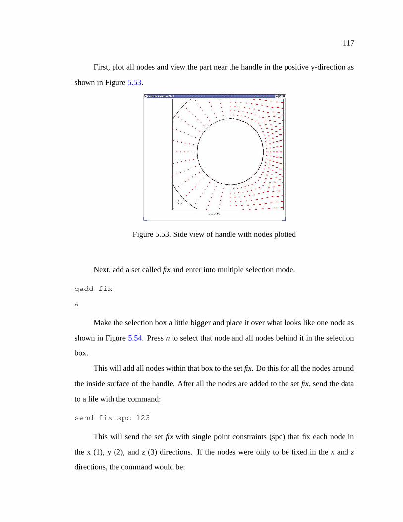
117
First, plot all nodes and view the part near the handle in the positive y-direction as
shown in Figure 5.53.
Figure 5.53. Side view of handle with nodes plotted
Next, add a set called fix and enter into multiple selection mode.
qadd fix
a
Make the selection box a little bigger and place it over what looks like one node as
shown in Figure 5.54. Press n to select that node and all nodes behind it in the selection
box.
This will add all nodes within that box to the set fix. Do this for all the nodes around
the inside surface of the handle. After all the nodes are added to the set fix, send the data
to a file with the command:
send fix spc 123
This will send the set fix with single point constraints (spc) that fix each node in
the x (1), y (2), and z (3) directions. If the nodes were only to be fixed in the x and z
directions, the command would be:
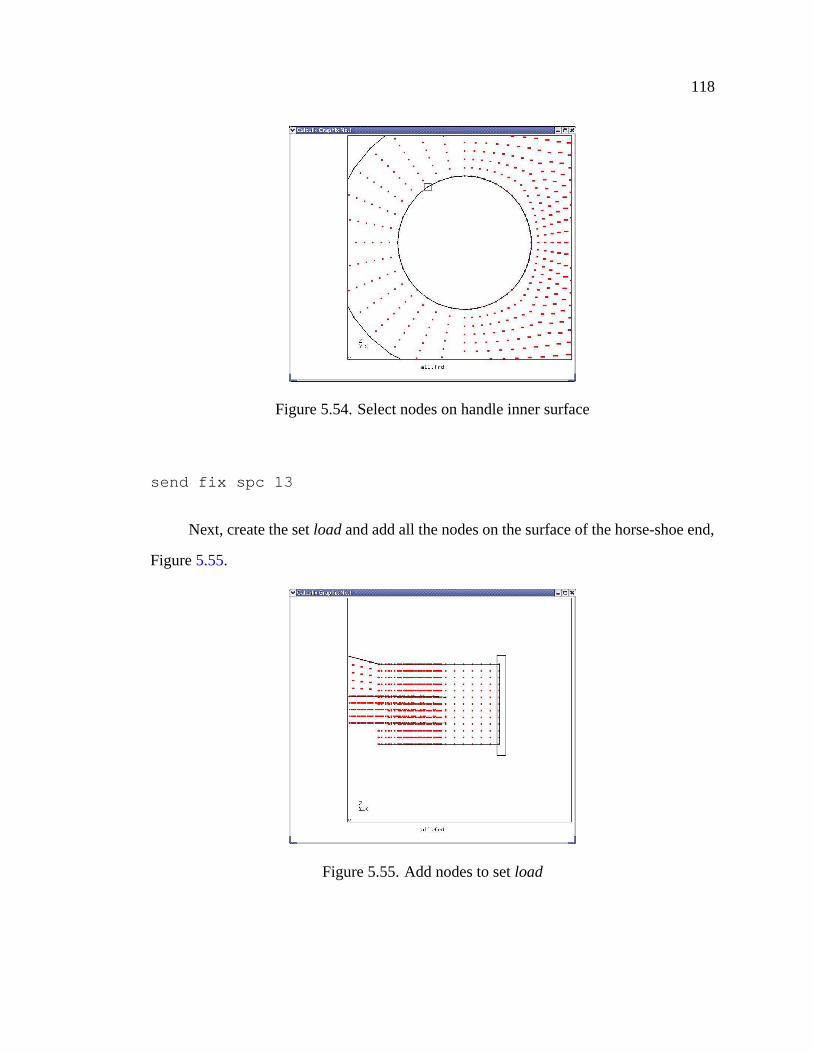
118
Figure 5.54. Select nodes on handle inner surface
send fix spc 13
Next, create the set load and add all the nodes on the surface of the horse-shoe end,
Figure 5.55.
Figure 5.55. Add nodes to set load
119
A 130 lbf load will be applied to the end of the horse-shoe surface. Since there are
130 nodes on this surface, simply apply a -1 lbf load to each node in the z-direction.
send load force 0 0 -1
Finally, send all the element and nodal data to a .msh file. This will contain the
element and nodal data in a format readable by CaluliX CrunchiX.
send all abq
Now that all necessary files are created that define the part, the input deck can be
created. The input deck contains the element and nodal data, the boundary conditions,
loading conditions, material definitions, the type of analysis, and what data to print out
for elements and nodes. The input deck for this run is seen in Appendix D
5.2.4 Run Analysis
After the input deck is created, the analysis can now be performed. Simply type at
the command line:
redboots@apollo> ccx_1.1 -i all.inp
all.inp is the name of the input deck file. After the analysis has completed, several files
will be created. The file ending in the extension frd contains the results that are available.
For this test node displacement and element stress are computed. To view the results,
type:
redboots@apollo> cgx all.frd
On the left hand side of the CalculiX GraphiX interface, left-click the mouse, select
Datasets, then Stress. Next, left-click on the left side of the CalculiX interface, select
Datasets, Entity, and then Mises. This will plot the von Mises stress for the part, Figure
5.56
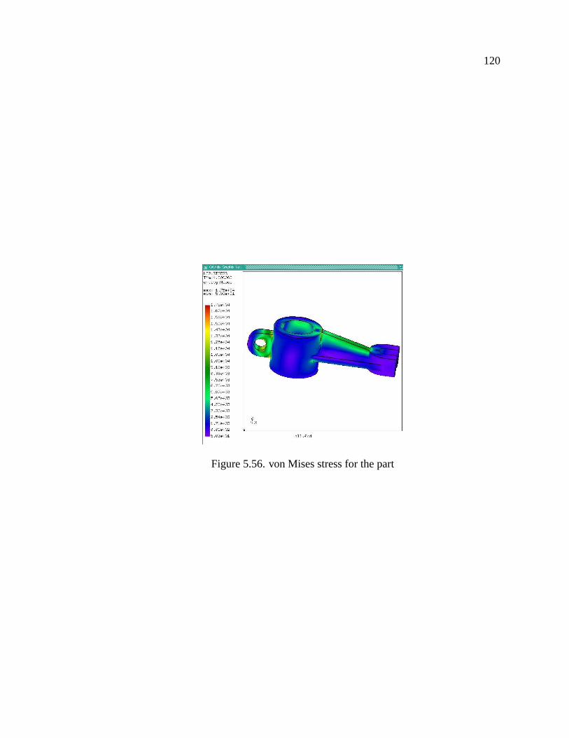
120
Figure 5.56. von Mises stress for the part
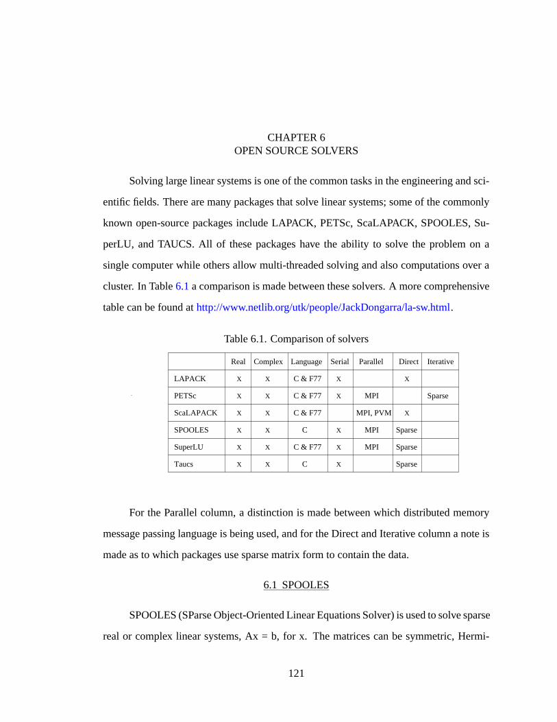
CHAPTER 6OPEN SOURCE SOLVERS
Solving large linear systems is one of the common tasks in the engineering and sci-
entific fields. There are many packages that solve linear systems; some of the commonly
known open-source packages include LAPACK, PETSc, ScaLAPACK, SPOOLES, Su-
perLU, and TAUCS. All of these packages have the ability to solve the problem on a
single computer while others allow multi-threaded solving and also computations over a
cluster. In Table 6.1 a comparison is made between these solvers. A more comprehensive
table can be found at http://www.netlib.org/utk/people/JackDongarra/la-sw.html.
Table 6.1. Comparison of solvers
ComplexReal Language Serial
LAPACK
Taucs
SuperLU
SPOOLES
ScaLAPACK
PETSc
X
X
X
X
X
X
X
X
X
X
X C & F77
C & F77
C & F77
C
C
X
X
X
X
X
X
C & F77
MPI, PVM
IterativeParallel Direct
MPI
MPI
MPI
X
X
Sparse
Sparse
Sparse
Sparse
For the Parallel column, a distinction is made between which distributed memory
message passing language is being used, and for the Direct and Iterative column a note is
made as to which packages use sparse matrix form to contain the data.
6.1 SPOOLES
SPOOLES (SParse Object-Oriented Linear Equations Solver) is used to solve sparse
real or complex linear systems, Ax = b, for x. The matrices can be symmetric, Hermi-
121
122
tian, square non-symmetric, or overdetermined [34]. SPOOLES can use either QR or
LU factorization in serial, multi-threaded, or parallel environments. SPOOLES could
be considered a medium size program with over 120,000 lines of code. Being Object
Oriented (OO), there are thirty-eight objects and over 1300 different functions with each
object knowing and operating on itself and knowing very little about other objects [35].
SPOOLES was supported in part by DARPA with contributions by Cleve Ashcraft, Daniel
Pierce, David K. Wah, and Jason Wu.
6.1.1 Objects in SPOOLES
SPOOLES is Object Oriented software written in the C language. Object Oriented
programming uses objects that interact with each other. Objects provide modularity and
structure to the program and they contain both data and functions [36].
The objects that make up SPOOLES are divided into three categories, utility, or-
dering, and numeric. The utility objects have several uses such as storing and operating
on dense matrices, creating storage for real and complex vectors, generating a random
number, and storing permutation vectors. The ordering objects can represent a partition
of a graph during nested dissection, model an elimination tree for factorization, represent
the graph of a matrix, and provide an ordering based on minimum degree, multi-section,
or nested dissection algorithms. Numeric objects can assemble a sparse matrix, store and
operate on a front during factorization, hold submatrix data and operate on them, and
numeric objects also solve linear systems [37]. A complete list of the available utility,
ordering, and numeric objects are seen in Tables 6.2, 6.3 and 6.4 respectively.
6.1.2 Steps to Solve Equations
There are four main steps to solving equations in SPOOLES - communicate, re-
order, factor, and solve [34]. In later sections these steps will be explained in more de-
tail for solving in serial and parallel environments. The multi-threaded capabilities of
SPOOLES will not be looked at because the goal is to compare the methods that we are
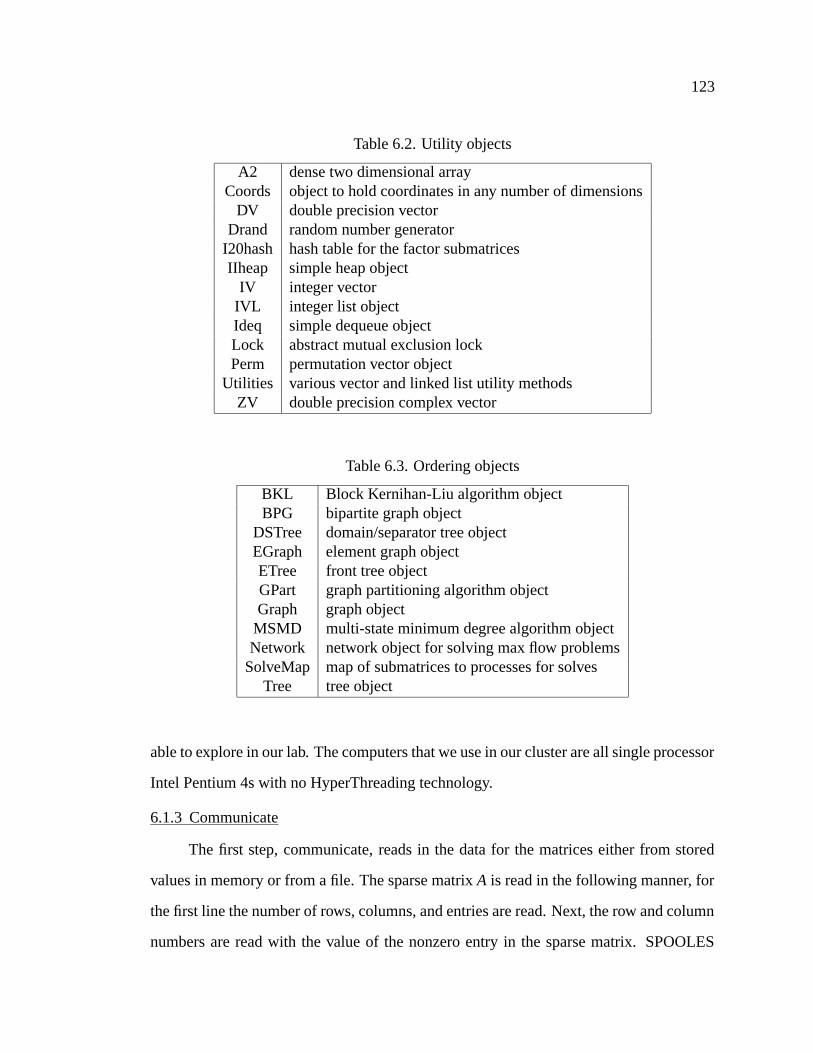
123
Table 6.2. Utility objects
A2 dense two dimensional arrayCoords object to hold coordinates in any number of dimensions
DV double precision vectorDrand random number generator
I20hash hash table for the factor submatricesIIheap simple heap object
IV integer vectorIVL integer list objectIdeq simple dequeue objectLock abstract mutual exclusion lockPerm permutation vector object
Utilities various vector and linked list utility methodsZV double precision complex vector
Table 6.3. Ordering objects
BKL Block Kernihan-Liu algorithm objectBPG bipartite graph object
DSTree domain/separator tree objectEGraph element graph objectETree front tree objectGPart graph partitioning algorithm objectGraph graph object
MSMD multi-state minimum degree algorithm objectNetwork network object for solving max flow problems
SolveMap map of submatrices to processes for solvesTree tree object
able to explore in our lab. The computers that we use in our cluster are all single processor
Intel Pentium 4s with no HyperThreading technology.
6.1.3 Communicate
The first step, communicate, reads in the data for the matrices either from stored
values in memory or from a file. The sparse matrix A is read in the following manner, for
the first line the number of rows, columns, and entries are read. Next, the row and column
numbers are read with the value of the nonzero entry in the sparse matrix. SPOOLES
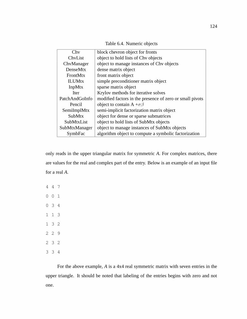
124
Table 6.4. Numeric objects
Chv block chevron object for frontsChvList object to hold lists of Chv objects
ChvManager object to manage instances of Chv objectsDenseMtx dense matrix objectFrontMtx front matrix objectILUMtx simple preconditioner matrix objectInpMtx sparse matrix object
Iter Krylov methods for iterative solvesPatchAndGoInfo modified factors in the presence of zero or small pivots
Pencil object to contain A +σβ
SemiImplMtx semi-implicit factorization matrix objectSubMtx object for dense or sparse submatrices
SubMtxList object to hold lists of SubMtx objectsSubMtxManager object to manage instances of SubMtx objects
SymbFac algorithm object to compute a symbolic factorization
only reads in the upper triangular matrix for symmetric A. For complex matrices, there
are values for the real and complex part of the entry. Below is an example of an input file
for a real A.
4 4 7
0 0 1
0 3 4
1 1 3
1 3 2
2 2 9
2 3 2
3 3 4
For the above example, A is a 4x4 real symmetric matrix with seven entries in the
upper triangle. It should be noted that labeling of the entries begins with zero and not
one.
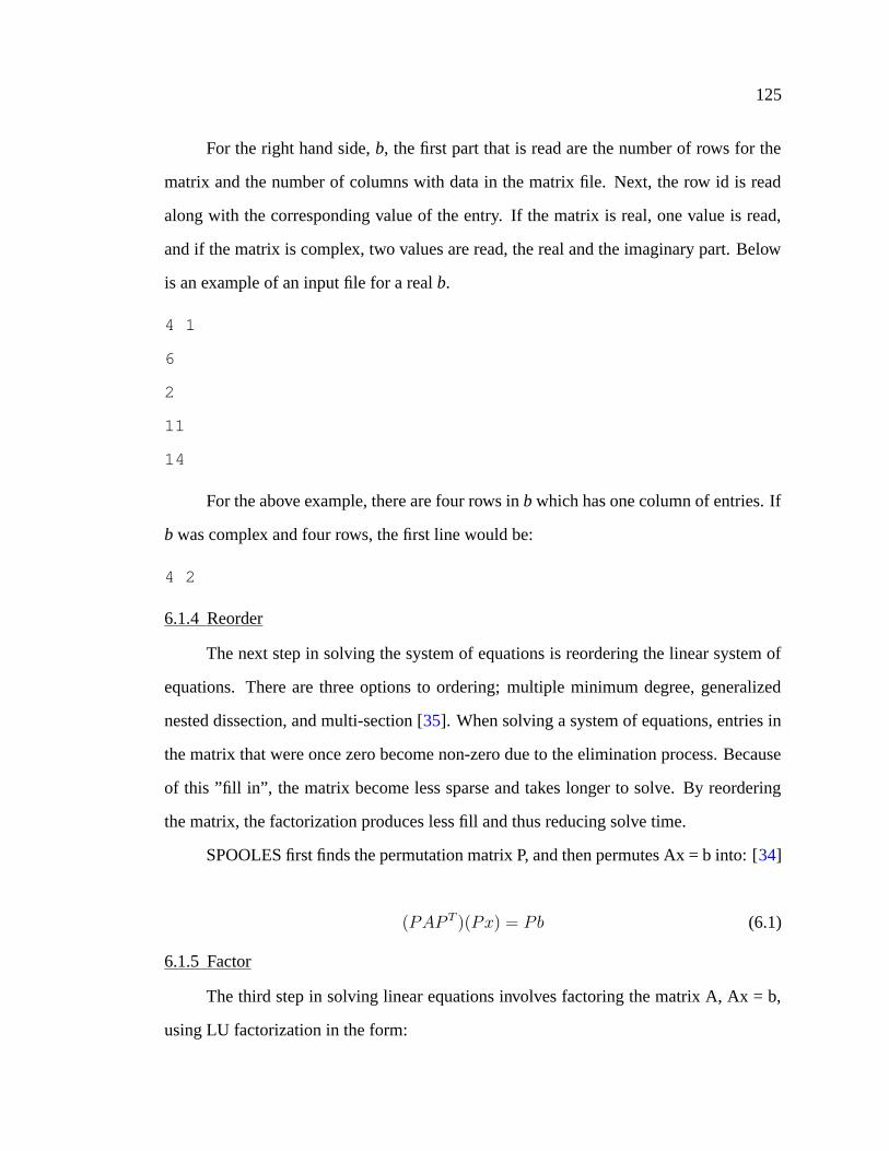
125
For the right hand side, b, the first part that is read are the number of rows for the
matrix and the number of columns with data in the matrix file. Next, the row id is read
along with the corresponding value of the entry. If the matrix is real, one value is read,
and if the matrix is complex, two values are read, the real and the imaginary part. Below
is an example of an input file for a real b.
4 1
6
2
11
14
For the above example, there are four rows in b which has one column of entries. If
b was complex and four rows, the first line would be:
4 2
6.1.4 Reorder
The next step in solving the system of equations is reordering the linear system of
equations. There are three options to ordering; multiple minimum degree, generalized
nested dissection, and multi-section [35]. When solving a system of equations, entries in
the matrix that were once zero become non-zero due to the elimination process. Because
of this ”fill in”, the matrix become less sparse and takes longer to solve. By reordering
the matrix, the factorization produces less fill and thus reducing solve time.
SPOOLES first finds the permutation matrix P, and then permutes Ax = b into: [34]
(PAP T )(Px) = Pb (6.1)
6.1.5 Factor
The third step in solving linear equations involves factoring the matrix A, Ax = b,
using LU factorization in the form:
126
A = LDU (6.2)
or
A = UT DU (6.3)
since A is symmetric.
SPOOLES uses Crout’s algorithm for performing the LU decomposition, where D
is a diagonal matrix, and U is an upper triangular matrix with 1’s along the diagonal.
Crout’s algorithm is further explained in [38]. During the solve, the user has a choice of
using pivoting to ensure numerical stability. Pivoting is a process of sorting rows and/or
columns of a matrix so that the pivot is the largest entry in the column for partial pivoting
and largest entry in the matrix for complete pivoting. For SPOOLES, the magnitude of
entries in both L and U are bounded by a user specified value, the recommended values
are 100 or 1000 [35]. The pivoting method used is SPOOLES is explained in more detail
in [39].
6.1.6 Solve
The last step involved is solving the linear equations using forward and backsolving.
Substituting Eq. 6.3 into Eq. 6.1 and solving the following for y:
UT y = b (6.4)
Then backsolve Eq. 6.5 to get x.
Ux = y (6.5)
127
6.2 Code to Solve Equations
There are three environments in which SPOOLES can solve equations: in serial, us-
ing multiple threads, and in parallel. When the serial drivers are used, only one processor
is used solving the problem sequentially. This environment is ideal for relatively small
problems where the computational time is within a user defined acceptable period. Multi-
threaded SPOOLES allows the application to handle more than one operation at a time
by separating tasks into individual threads. A multi-threaded application may offer some
benefits on a single-processor machine, such as an Intel Pentium 4 with HyperThread-
ing, but a multiple processor computer is much more suited to taking full advantage of
multiple threads. The parallel routines of SPOOLES were originally designed to operate
on MPP machines with a fast network interconnect but with increasing bandwidth and
reduction of latency of current networking equipment, it is viable for SPOOLES to be run
on multiple computers arranged in a cluster. By using multiple computers connected by
a fast network and coding applications utilizing a parallel interface such as MPI, certain
problems may be solved in less time than with a single computer.
6.3 Serial Code
Initially, the driver that CalculiX uses in solving equations connects to the serial
routines supplied in SPOOLES. The code used by CalculiX is seen in Appendix E.1. The
steps used by CalculiX are included in the four steps that SPOOLES divides the work
into.
6.3.1 Communicate
The first step, communicate, reads and stores the entries of the matrix A, Ax = b.
This is carried out by the following code segment.
mtxA = InpMtx_new() ;
InpMtx_init(mtxA, INPMTX_BY_ROWS, type, nent, neqns) ;
128
for(row=0;row<nrow;row++){
InpMtx_inputRealEntry(mtxA,row,row,ad[row]);
for(ipo=ipoint;ipo<ipoint+icol[row];ipo++){
col=irow[ipo]-1;
InpMtx_inputRealEntry(mtxA,row,col,au[ipo]);
}
ipoint=ipoint+icol[row];
}
The first object used is InpMtx. To use the InpMtx object to store entries of a sparse
matrix, the following steps are carried out. First, storage is allocated for the object InpMtx
with a call to InpMtx new() and InpMtx is initialized by a call to InpMtx init(). The first
argument of InpMtx init() is a pointer to the InpMtx object, mtxA.
• The second argument sets how mtxA is stored.
• The third argument, type, lets InpMtx init() know if the matrix is real or complex.
• The forth argument, nent, is an estimate of the number of nonzero entries in the
matrix.
• The fifth argument, neqns, is the number of rows or columns.
Next, entries of the matrix object are placed by InpMtx inputRealEntry(). If a com-
plex matrix was used, InpMtx inputRealEntry() would be replaced by
InpMtx inputComplexEntry() and its appropriate arguments. The argument ad[] contains
the diagonal element for a particular row, au[] contains some sub-diagonal entry of the
matrix, and icol[i] contains the number of nonzero subdiagonal entries in column i. ad[],
au[], and icol[] are functions that are defined within CalculiX and relay the matrix infor-
mation to the SPOOLES solver.
129
The second part of communicate, reading and storing the entries of b, will be per-
formed later.
6.3.2 Reorder
The second step of solving a linear system of equations with CalculiX is to find
a low-fill ordering to reduce storage and computational requirements of a sparse matrix
factorization. This falls into the reorder step. The code that performs this operation is
seen below.
graph = Graph_new() ;adjIVL = InpMtx_fullAdjacency(mtxA) ;nedges = IVL_tsize(adjIVL) ;Graph_init2(graph, 0, neqns, 0, nedges, neqns, nedges, adjIVL,
NULL, NULL) ;maxdomainsize=800;maxzeros=1000;maxsize=64;frontETree=orderViaBestOfNDandMS(graph,maxdomainsize,maxzeros,
maxsize,seed,msglvl,msgFile);
The above code initializes the Graph object which is used to represent the graph of
a matrix. This step also uses the IVL object to represent adjacency lists, one edge list for
each vertex in the graph [37]. (maybe show example) The first line Graph new() allocates
storage for the Graph structure. The second line creates and returns an object that holds
the full adjacency structure of
A + AT
This above structure is used because the LU factorization of SPOOLES works with sym-
metric matrices. The ordering that serial CalculiX uses is determined by finding the better
of two methods - nested dissection and multi-section. Much of the work used to find ei-
ther a nested dissection or multi-section ordering is identical, so little more time is used
[40]. orderViaBestOfNDandMS() splits a subgraph if it has more vertices than the max-
domainsize argument and also transforms the front tree using the maxzeros and maxsize
parameters [40]. These will be explained later.
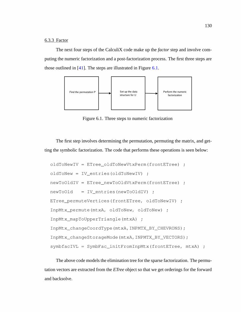
130
6.3.3 Factor
The next four steps of the CalculiX code make up the factor step and involve com-
puting the numeric factorization and a post-factorization process. The first three steps are
those outlined in [41]. The steps are illustrated in Figure 6.1.
Figure 6.1. Three steps to numeric factorization
The first step involves determining the permutation, permuting the matrix, and get-
ting the symbolic factorization. The code that performs these operations is seen below:
oldToNewIV = ETree_oldToNewVtxPerm(frontETree) ;
oldToNew = IV_entries(oldToNewIV) ;
newToOldIV = ETree_newToOldVtxPerm(frontETree) ;
newToOld = IV_entries(newToOldIV) ;
ETree_permuteVertices(frontETree, oldToNewIV) ;
InpMtx_permute(mtxA, oldToNew, oldToNew) ;
InpMtx_mapToUpperTriangle(mtxA) ;
InpMtx_changeCoordType(mtxA,INPMTX_BY_CHEVRONS);
InpMtx_changeStorageMode(mtxA,INPMTX_BY_VECTORS);
symbfacIVL = SymbFac_initFromInpMtx(frontETree, mtxA) ;
The above code models the elimination tree for the sparse factorization. The permu-
tation vectors are extracted from the ETree object so that we get orderings for the forward
and backsolve.
131
Next, the front matrix object is initialized. This is performed by the following code:
frontmtx = FrontMtx_new() ;mtxmanager = SubMtxManager_new() ;SubMtxManager_init(mtxmanager, NO_LOCK, 0) ;FrontMtx_init(frontmtx, frontETree, symbfacIVL, type, symmetryflag,
FRONTMTX_DENSE_FRONTS, pivotingflag, NO_LOCK, 0, NULL,mtxmanager, msglvl, msgFile) ;
In a sequential frontal solver for finite-element codes, a ’front’ sweeps through
the mesh, one element at a time, assembling the element stiffness matrices into a so-
called ’frontal’ matrix [42]. FrontMtx new() allocates storage for the FrontMtx structure,
SubMtxManager new() allocates storage for the SubMtxManger structure, and the front
matrix is initialized by FrontMtx init(). SubMtxManager handles multiple instances of the
SubMtx object. The SubMtx object holds and operates with double precision or complex
submatrices of a sparse matrix. FrontMtx init() initializes the object, and allocating and
initializing the internal objects as necessary [37].
The numeric factorization is then calculated with the following code:
chvmanager = ChvManager_new() ;ChvManager_init(chvmanager, NO_LOCK, 1) ;DVfill(10, cpus, 0.0) ;IVfill(20, stats, 0) ;rootchv = FrontMtx_factorInpMtx(frontmtx, mtxA, tau, 0.0,chvmanager, &error,cpus, stats, msglvl, msgFile) ;ChvManager_free(chvmanager) ;
The Chv object is the block chevron object that is used to store and operate on a
front during a sparse factorization. The word ”chevron” was chosen by the authors to
describe the front because if you rotate Figure 6.2 forty-five degrees clockwise the entries
resemble the chevron insignia of enlisted personnel in the armed forces. Also ”block”
emphasizes that the diagonal may have multiple entries [37].
ChvManager new() allocates memory for the ChvManager structure, while Chv-
Manager init() initializes the object. FrontMtx factorInpMtx() performs a serial factor-
ization of mtxA with the following parameters:
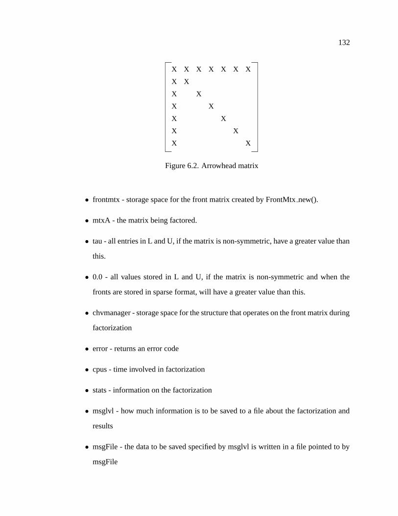
132
X
X
X
X
X
X X X X
X
X
X
X
X
X
X
X
X
X
Figure 6.2. Arrowhead matrix
• frontmtx - storage space for the front matrix created by FrontMtx new().
• mtxA - the matrix being factored.
• tau - all entries in L and U, if the matrix is non-symmetric, have a greater value than
this.
• 0.0 - all values stored in L and U, if the matrix is non-symmetric and when the
fronts are stored in sparse format, will have a greater value than this.
• chvmanager - storage space for the structure that operates on the front matrix during
factorization
• error - returns an error code
• cpus - time involved in factorization
• stats - information on the factorization
• msglvl - how much information is to be saved to a file about the factorization and
results
• msgFile - the data to be saved specified by msglvl is written in a file pointed to by
msgFile
133
The last part of the factorization process involves permuting the row and column
adjacency objects, permuting the lower and upper matrices, and updating the block adja-
cency objects [37]. This is carried out by the following code:
FrontMtx_postProcess(frontmtx, msglvl, msgFile) ;
6.3.4 Communicate B
Next, the second part of communicate, reading the the right hand side of Ax = b, b,
is performed. This is accomplished by the following code:
mtxB = DenseMtx_new() ;
DenseMtx_init(mtxB, type, 0, 0, neqns, nrhs, 1, neqns) ;
DenseMtx_zero(mtxB) ;
for ( jrow = 0 ; jrow < nrow ; jrow++ ) {
for ( jrhs = 0 ; jrhs < nrhs ; jrhs++ ) {
DenseMtx_setRealEntry(mtxB, jrow, jrhs, b[jrow]) ;
}
}
First, DenseMtx new() is called which allocates storage for the DenseMtx object.
The DenseMtx object contains a dense matrix, not stored in sparse format, along with row
and column indices. Next, DenseMtx init() initializes the DenseMtx object and calculates
the bytes required for the workspace. The following parameters are specified during
DenseMtx init [37].
• mtxB - space created for the dense matrix B
• type - specifies whether the matrix is real or complex
• 3rd and 4th arguments - specify row and column ids of the matrix
134
• neqns - number of equations and also equal to the number of rows, nrow, in the
matrix
• nrhs - number of columns in the matrix
• 7th and 8th arguments - the dense matrix is stored in column major format so the
row stride is 1 and the column stride is the number of equations or rows
Lastly, the entries in row jrow and column jrhs are given the value b[jrow] with the
call to Densemtx setRealEntry().
The next step involves permuting the right hand side into the new ordering. When a
low-fill ordering is found for the sparse matrix A, the new ordering arrangement is applied
to the dense matrix b. This is performed by the following code:
DenseMtx_permuteRows(mtxB, oldToNewIV) ;
6.3.5 Solve
The last step, solve, is to solve the linear system for x. This is performed by the
following code.
mtxX = DenseMtx_new() ;DenseMtx_init(mtxX, type, 0, 0, neqns, nrhs, 1, neqns) ;DenseMtx_zero(mtxX) ;FrontMtx_solve(frontmtx,mtxX,mtxB,mtxmanager,cpus,msglvl,msgFile) ;
The first line allocates storage for the DenseMtx structure and assigns the storage
space to mtxX. DenseMtx init initializes the DenseMtx object and calculates the number
of bytes required for the workspace. Next, DenseMtx zero() zeros the entries in the matrix
mtxX. Finally, the system of equations is solved by FrontMtx solve(). The parameters are
as follows:
• frontmtx - storage space for the front matrix
• mtxX - entries of x, Ax = b, are written to mtxX
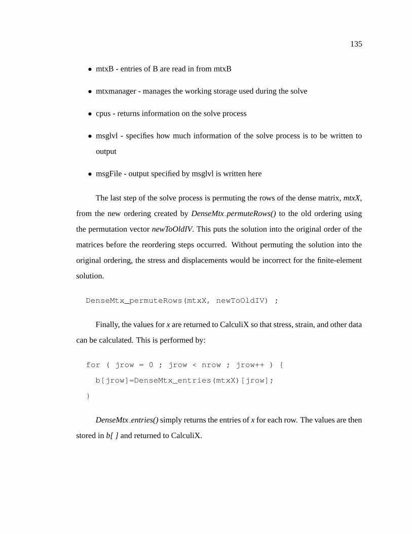
135
• mtxB - entries of B are read in from mtxB
• mtxmanager - manages the working storage used during the solve
• cpus - returns information on the solve process
• msglvl - specifies how much information of the solve process is to be written to
output
• msgFile - output specified by msglvl is written here
The last step of the solve process is permuting the rows of the dense matrix, mtxX,
from the new ordering created by DenseMtx permuteRows() to the old ordering using
the permutation vector newToOldIV. This puts the solution into the original order of the
matrices before the reordering steps occurred. Without permuting the solution into the
original ordering, the stress and displacements would be incorrect for the finite-element
solution.
DenseMtx_permuteRows(mtxX, newToOldIV) ;
Finally, the values for x are returned to CalculiX so that stress, strain, and other data
can be calculated. This is performed by:
for ( jrow = 0 ; jrow < nrow ; jrow++ ) {
b[jrow]=DenseMtx_entries(mtxX)[jrow];
}
DenseMtx entries() simply returns the entries of x for each row. The values are then
stored in b[ ] and returned to CalculiX.
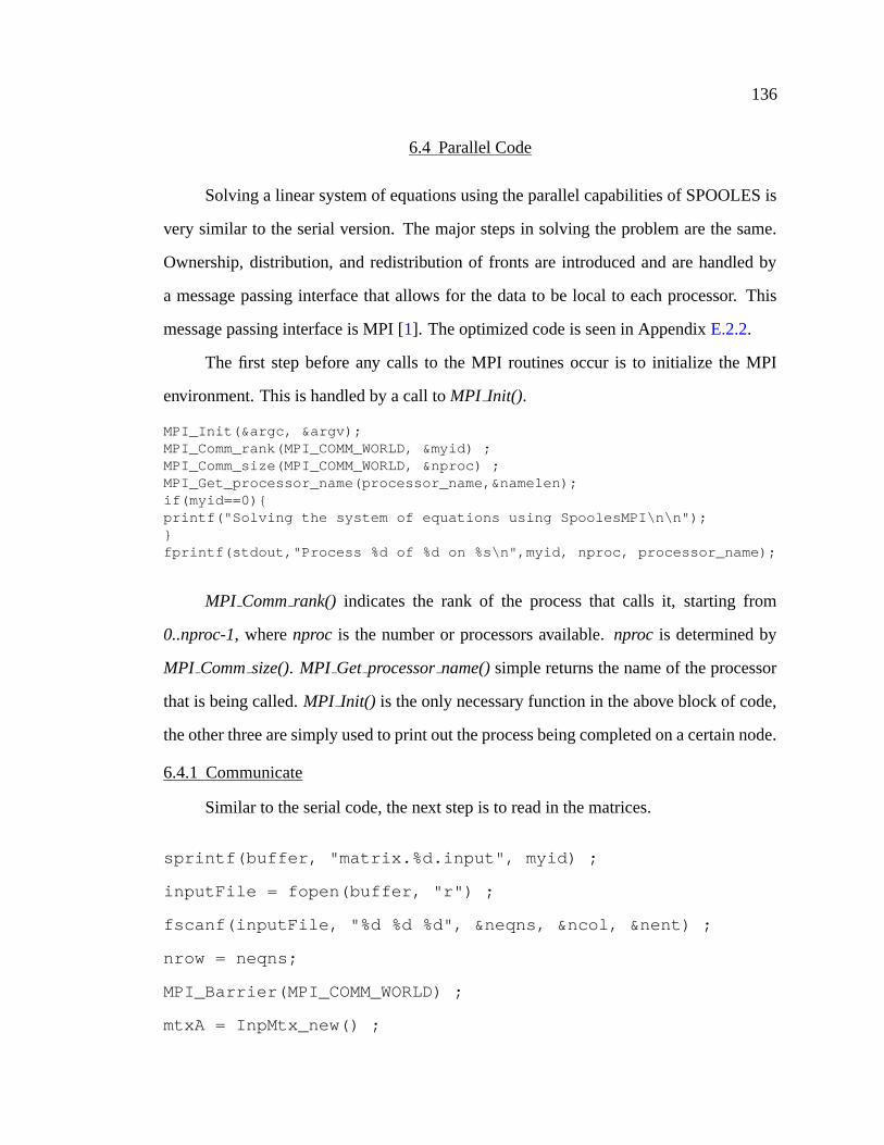
136
6.4 Parallel Code
Solving a linear system of equations using the parallel capabilities of SPOOLES is
very similar to the serial version. The major steps in solving the problem are the same.
Ownership, distribution, and redistribution of fronts are introduced and are handled by
a message passing interface that allows for the data to be local to each processor. This
message passing interface is MPI [1]. The optimized code is seen in Appendix E.2.2.
The first step before any calls to the MPI routines occur is to initialize the MPI
environment. This is handled by a call to MPI Init().
MPI_Init(&argc, &argv);MPI_Comm_rank(MPI_COMM_WORLD, &myid) ;MPI_Comm_size(MPI_COMM_WORLD, &nproc) ;MPI_Get_processor_name(processor_name,&namelen);if(myid==0){printf("Solving the system of equations using SpoolesMPI\n\n");}fprintf(stdout,"Process %d of %d on %s\n",myid, nproc, processor_name);
MPI Comm rank() indicates the rank of the process that calls it, starting from
0..nproc-1, where nproc is the number or processors available. nproc is determined by
MPI Comm size(). MPI Get processor name() simple returns the name of the processor
that is being called. MPI Init() is the only necessary function in the above block of code,
the other three are simply used to print out the process being completed on a certain node.
6.4.1 Communicate
Similar to the serial code, the next step is to read in the matrices.
sprintf(buffer, "matrix.%d.input", myid) ;
inputFile = fopen(buffer, "r") ;
fscanf(inputFile, "%d %d %d", &neqns, &ncol, &nent) ;
nrow = neqns;
MPI_Barrier(MPI_COMM_WORLD) ;
mtxA = InpMtx_new() ;
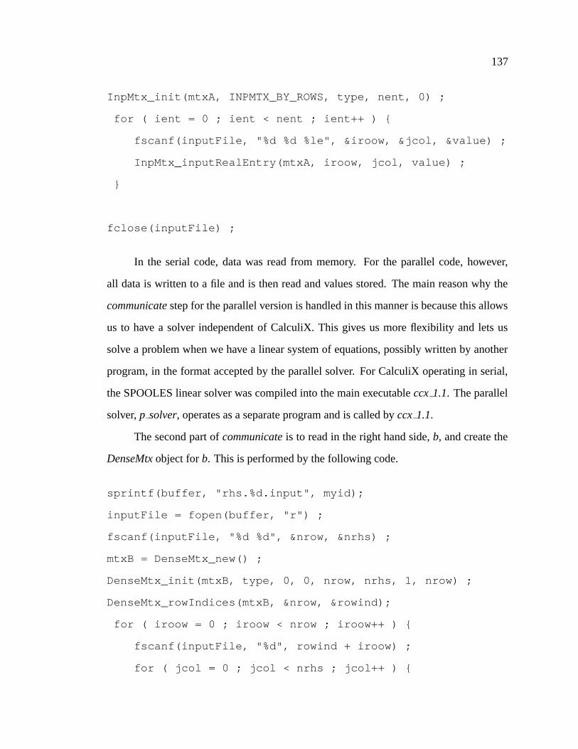
137
InpMtx_init(mtxA, INPMTX_BY_ROWS, type, nent, 0) ;
for ( ient = 0 ; ient < nent ; ient++ ) {
fscanf(inputFile, "%d %d %le", &iroow, &jcol, &value) ;
InpMtx_inputRealEntry(mtxA, iroow, jcol, value) ;
}
fclose(inputFile) ;
In the serial code, data was read from memory. For the parallel code, however,
all data is written to a file and is then read and values stored. The main reason why the
communicate step for the parallel version is handled in this manner is because this allows
us to have a solver independent of CalculiX. This gives us more flexibility and lets us
solve a problem when we have a linear system of equations, possibly written by another
program, in the format accepted by the parallel solver. For CalculiX operating in serial,
the SPOOLES linear solver was compiled into the main executable ccx 1.1. The parallel
solver, p solver, operates as a separate program and is called by ccx 1.1.
The second part of communicate is to read in the right hand side, b, and create the
DenseMtx object for b. This is performed by the following code.
sprintf(buffer, "rhs.%d.input", myid);
inputFile = fopen(buffer, "r") ;
fscanf(inputFile, "%d %d", &nrow, &nrhs) ;
mtxB = DenseMtx_new() ;
DenseMtx_init(mtxB, type, 0, 0, nrow, nrhs, 1, nrow) ;
DenseMtx_rowIndices(mtxB, &nrow, &rowind);
for ( iroow = 0 ; iroow < nrow ; iroow++ ) {
fscanf(inputFile, "%d", rowind + iroow) ;
for ( jcol = 0 ; jcol < nrhs ; jcol++ ) {
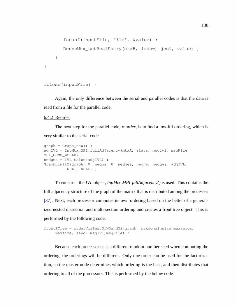
138
fscanf(inputFile, "%le", &value) ;
DenseMtx_setRealEntry(mtxB, iroow, jcol, value) ;
}
}
fclose(inputFile) ;
Again, the only difference between the serial and parallel codes is that the data is
read from a file for the parallel code.
6.4.2 Reorder
The next step for the parallel code, reorder, is to find a low-fill ordering, which is
very similar to the serial code.
graph = Graph_new() ;adjIVL = InpMtx_MPI_fullAdjacency(mtxA, stats, msglvl, msgFile,MPI_COMM_WORLD) ;nedges = IVL_tsize(adjIVL) ;Graph_init2(graph, 0, neqns, 0, nedges, neqns, nedges, adjIVL,
NULL, NULL) ;
To construct the IVL object, InpMtx MPI fullAdjacency() is used. This contains the
full adjacency structure of the graph of the matrix that is distributed among the processes
[37]. Next, each processor computes its own ordering based on the better of a general-
ized nested dissection and multi-section ordering and creates a front tree object. This is
performed by the following code.
frontETree = orderViaBestOfNDandMS(graph, maxdomainsize,maxzeros,maxsize, seed, msglvl,msgFile) ;
Because each processor uses a different random number seed when computing the
ordering, the orderings will be different. Only one order can be used for the factoriza-
tion, so the master node determines which ordering is the best, and then distributes that
ordering to all of the processors. This is performed by the below code.
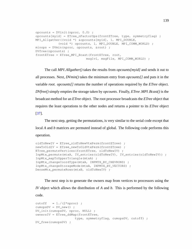
139
opcounts = DVinit(nproc, 0.0) ;opcounts[myid] = ETree_nFactorOps(frontETree, type, symmetryflag) ;MPI_Allgather((void *) &opcounts[myid], 1, MPI_DOUBLE,
(void *) opcounts, 1, MPI_DOUBLE, MPI_COMM_WORLD) ;minops = DVmin(nproc, opcounts, &root) ;DVfree(opcounts) ;frontETree = ETree_MPI_Bcast(frontETree, root,
msglvl, msgFile, MPI_COMM_WORLD) ;
The call MPI Allgather() takes the results from opcounts[myid] and sends it out to
all processes. Next, DVmin() takes the minimum entry from opcounts[] and puts it in the
variable root. opcounts[] returns the number of operations required by the ETree object.
DVfree() simply empties the storage taken by opcounts. Finally, ETree MPI Bcast() is the
broadcast method for an ETree object. The root processor broadcasts the ETree object that
requires the least operations to the other nodes and returns a pointer to its ETree object
[37].
The next step, getting the permutations, is very similar to the serial code except that
local A and b matrices are permuted instead of global. The following code performs this
operation.
oldToNewIV = ETree_oldToNewVtxPerm(frontETree) ;newToOldIV = ETree_newToOldVtxPerm(frontETree) ;ETree_permuteVertices(frontETree, oldToNewIV) ;InpMtx_permute(mtxA, IV_entries(oldToNewIV), IV_entries(oldToNewIV)) ;InpMtx_mapToUpperTriangle(mtxA) ;InpMtx_changeCoordType(mtxA, INPMTX_BY_CHEVRONS) ;InpMtx_changeStorageMode(mtxA, INPMTX_BY_VECTORS) ;DenseMtx_permuteRows(mtxB, oldToNewIV) ;
The next step is to generate the owners map from vertices to processors using the
IV object which allows the distribution of A and b. This is performed by the following
code.
cutoff = 1./(2*nproc) ;cumopsDV = DV_new() ;DV_init(cumopsDV, nproc, NULL) ;ownersIV = ETree_ddMap(frontETree,
type, symmetryflag, cumopsDV, cutoff) ;DV_free(cumopsDV) ;
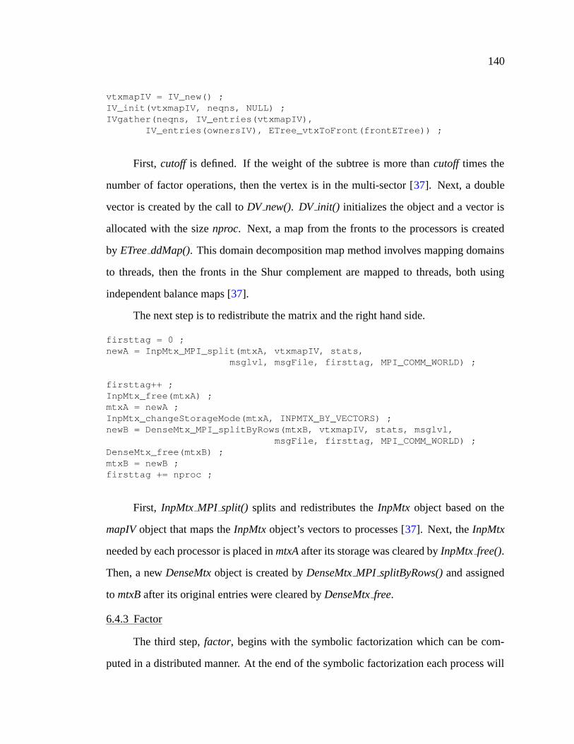
140
vtxmapIV = IV_new() ;IV_init(vtxmapIV, neqns, NULL) ;IVgather(neqns, IV_entries(vtxmapIV),
IV_entries(ownersIV), ETree_vtxToFront(frontETree)) ;
First, cutoff is defined. If the weight of the subtree is more than cutoff times the
number of factor operations, then the vertex is in the multi-sector [37]. Next, a double
vector is created by the call to DV new(). DV init() initializes the object and a vector is
allocated with the size nproc. Next, a map from the fronts to the processors is created
by ETree ddMap(). This domain decomposition map method involves mapping domains
to threads, then the fronts in the Shur complement are mapped to threads, both using
independent balance maps [37].
The next step is to redistribute the matrix and the right hand side.
firsttag = 0 ;newA = InpMtx_MPI_split(mtxA, vtxmapIV, stats,
msglvl, msgFile, firsttag, MPI_COMM_WORLD) ;
firsttag++ ;InpMtx_free(mtxA) ;mtxA = newA ;InpMtx_changeStorageMode(mtxA, INPMTX_BY_VECTORS) ;newB = DenseMtx_MPI_splitByRows(mtxB, vtxmapIV, stats, msglvl,
msgFile, firsttag, MPI_COMM_WORLD) ;DenseMtx_free(mtxB) ;mtxB = newB ;firsttag += nproc ;
First, InpMtx MPI split() splits and redistributes the InpMtx object based on the
mapIV object that maps the InpMtx object’s vectors to processes [37]. Next, the InpMtx
needed by each processor is placed in mtxA after its storage was cleared by InpMtx free().
Then, a new DenseMtx object is created by DenseMtx MPI splitByRows() and assigned
to mtxB after its original entries were cleared by DenseMtx free.
6.4.3 Factor
The third step, factor, begins with the symbolic factorization which can be com-
puted in a distributed manner. At the end of the symbolic factorization each process will
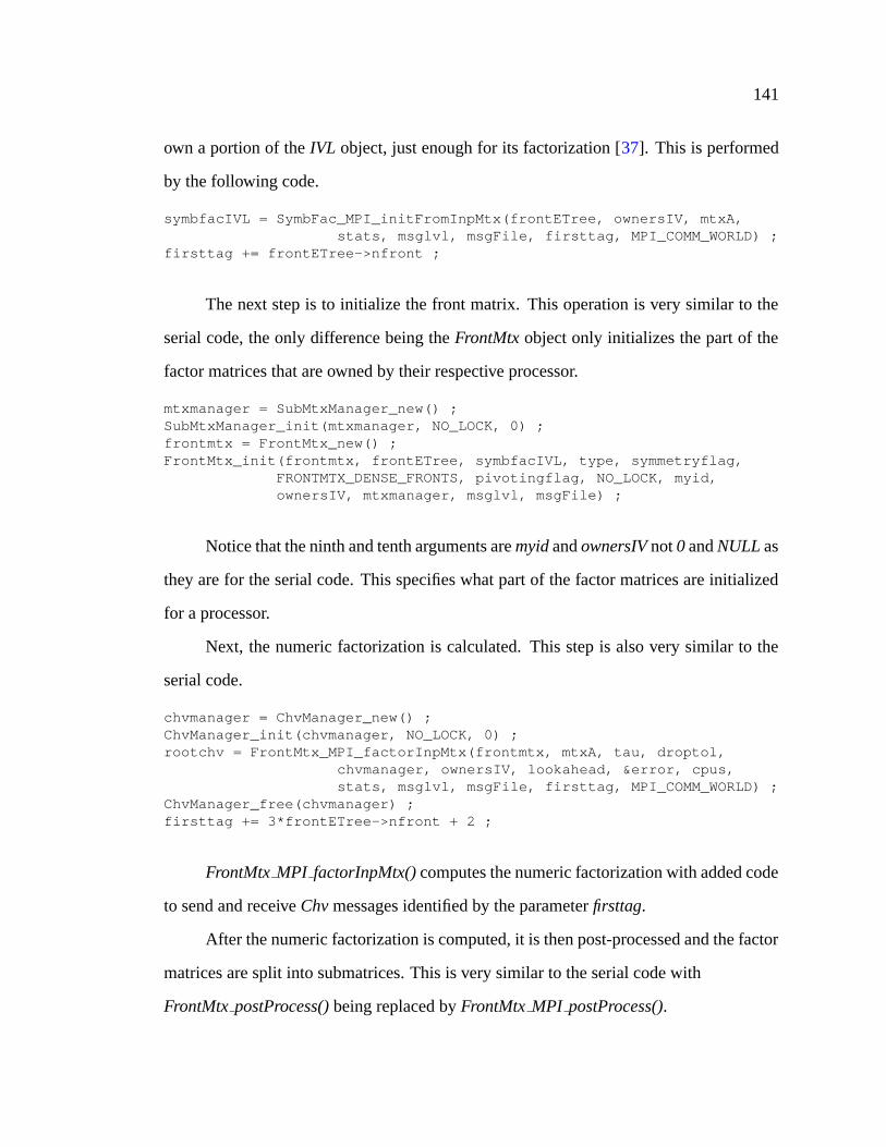
141
own a portion of the IVL object, just enough for its factorization [37]. This is performed
by the following code.
symbfacIVL = SymbFac_MPI_initFromInpMtx(frontETree, ownersIV, mtxA,stats, msglvl, msgFile, firsttag, MPI_COMM_WORLD) ;
firsttag += frontETree->nfront ;
The next step is to initialize the front matrix. This operation is very similar to the
serial code, the only difference being the FrontMtx object only initializes the part of the
factor matrices that are owned by their respective processor.
mtxmanager = SubMtxManager_new() ;SubMtxManager_init(mtxmanager, NO_LOCK, 0) ;frontmtx = FrontMtx_new() ;FrontMtx_init(frontmtx, frontETree, symbfacIVL, type, symmetryflag,
FRONTMTX_DENSE_FRONTS, pivotingflag, NO_LOCK, myid,ownersIV, mtxmanager, msglvl, msgFile) ;
Notice that the ninth and tenth arguments are myid and ownersIV not 0 and NULL as
they are for the serial code. This specifies what part of the factor matrices are initialized
for a processor.
Next, the numeric factorization is calculated. This step is also very similar to the
serial code.
chvmanager = ChvManager_new() ;ChvManager_init(chvmanager, NO_LOCK, 0) ;rootchv = FrontMtx_MPI_factorInpMtx(frontmtx, mtxA, tau, droptol,
chvmanager, ownersIV, lookahead, &error, cpus,stats, msglvl, msgFile, firsttag, MPI_COMM_WORLD) ;
ChvManager_free(chvmanager) ;firsttag += 3*frontETree->nfront + 2 ;
FrontMtx MPI factorInpMtx() computes the numeric factorization with added code
to send and receive Chv messages identified by the parameter firsttag.
After the numeric factorization is computed, it is then post-processed and the factor
matrices are split into submatrices. This is very similar to the serial code with
FrontMtx postProcess() being replaced by FrontMtx MPI postProcess().
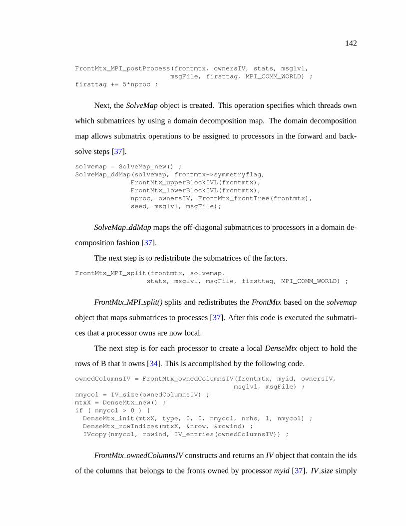
142
FrontMtx_MPI_postProcess(frontmtx, ownersIV, stats, msglvl,msgFile, firsttag, MPI_COMM_WORLD) ;
firsttag += 5*nproc ;
Next, the SolveMap object is created. This operation specifies which threads own
which submatrices by using a domain decomposition map. The domain decomposition
map allows submatrix operations to be assigned to processors in the forward and back-
solve steps [37].
solvemap = SolveMap_new() ;SolveMap_ddMap(solvemap, frontmtx->symmetryflag,
FrontMtx_upperBlockIVL(frontmtx),FrontMtx_lowerBlockIVL(frontmtx),nproc, ownersIV, FrontMtx_frontTree(frontmtx),seed, msglvl, msgFile);
SolveMap ddMap maps the off-diagonal submatrices to processors in a domain de-
composition fashion [37].
The next step is to redistribute the submatrices of the factors.
FrontMtx_MPI_split(frontmtx, solvemap,stats, msglvl, msgFile, firsttag, MPI_COMM_WORLD) ;
FrontMtx MPI split() splits and redistributes the FrontMtx based on the solvemap
object that maps submatrices to processes [37]. After this code is executed the submatri-
ces that a processor owns are now local.
The next step is for each processor to create a local DenseMtx object to hold the
rows of B that it owns [34]. This is accomplished by the following code.
ownedColumnsIV = FrontMtx_ownedColumnsIV(frontmtx, myid, ownersIV,msglvl, msgFile) ;
nmycol = IV_size(ownedColumnsIV) ;mtxX = DenseMtx_new() ;if ( nmycol > 0 ) {DenseMtx_init(mtxX, type, 0, 0, nmycol, nrhs, 1, nmycol) ;DenseMtx_rowIndices(mtxX, &nrow, &rowind) ;IVcopy(nmycol, rowind, IV_entries(ownedColumnsIV)) ;
FrontMtx ownedColumnsIV constructs and returns an IV object that contain the ids
of the columns that belongs to the fronts owned by processor myid [37]. IV size simply
143
returns the size of vector ownedColumnsIV, which is the distributed vector bmyid, where
myid is a particular processor. Next, the DenseMtx object is initialized by DenseMtx init()
and the number entries in IV entries(ownedColumnsIV) are copied from rowind to nmy-
col.
6.4.4 Solve
Next, the linear system is solved. This is performed in a manner very similarly to
the serial code.
solvemanager = SubMtxManager_new() ;SubMtxManager_init(solvemanager, NO_LOCK, 0) ;FrontMtx_MPI_solve(frontmtx, mtxX, mtxB, solvemanager, solvemap, cpus,
stats, msglvl, msgFile, firsttag, MPI_COMM_WORLD) ;SubMtxManager_free(solvemanager) ;
SubMtxManager new() initializes the SubMtx object manager. The SubMtx object
manager is similar to the ChvManager object in that the SubMtx object manager handles a
number of instances of SubMtx double precision matrix objects while ChvManager han-
dles a number of instances of Chv objects. There are two actions that can be taken by the
SubMtx manager: creating new and freeing objects, and recycling objects. SubMtxMan-
ager new() allocates storage for the SubMtxManager while SubMtxManager free() frees
up space for the SubMtxManager. For recycling of the objects, the manager keeps a list of
free objects ordered by descending size and when an object is needed, the list is searched
and the object with the required size is returned. FrontMtx MPI solve() performs the
forward and backsolves.
The last step is permuting the local matrix on each processor into the original order-
ing and assembling the final solution onto processor 0. This is performed by the following
code.
DenseMtx_permuteRows(mtxX, newToOldIV) ;IV_fill(vtxmapIV, 0) ;firsttag++ ;mtxX = DenseMtx_MPI_splitByRows(mtxX, vtxmapIV, stats, msglvl, \msgFile, firsttag, MPI_COMM_WORLD) ;

144
if ( myid == 0 ) {printf("%d\n", nrow);sprintf(buffer, "/home/apollo/hda8/CalculiX/ccx_1.1/src/ \p_solver/x.result");inputFile=fopen(buffer, "w");
for ( jrow = 0 ; jrow < ncol ; jrow++ ) {fprintf(inputFile, "%1.5e\n", DenseMtx_entries(mtxX)[jrow]);}fclose(inputFile);
}MPI_Finalize() ;
First, the rows are permuted back into the original ordering by using a new-to-old
permutation vector in the call to DenseMtx permuteRows. Next, the solution, mtxX is
assembled by a call to DenseMtx MPI splitByRows(). Then, the solution is written to a
file by calling DenseMtx entries() to return the entries. Finally, any program that uses
MPI needs a call to MPI Finalize() so that the MPI environment is terminated [14]. This
does not terminate the task but any call to a MPI function after MPI Finalize() returns an
error.
CHAPTER 7MATRIX ORDERINGS
In this chapter, three different matrix ordering algorithms, minimum degree, nested
dissection, and multi-section, will be discussed. Their advantages, disadvantages, and a
brief history of their development will also reviewed. By optimizing the ordering of the
sparse matrix a substantial decrease in time can be achieved during the solve [40].
7.1 Ordering Optimization
The ordering or graph partitioning of the linear system of equations is crucial for
performance of the parallel code. During Gaussian elimination, an entry in A that was
zero may become non-zero, termed fill-in. In general, fill-in is considered to be undesir-
able because it increases the amount of memory required to store the linear system and
increases processing power required to solve the problem [41]. Often, the size of the
problem that can be solved is limited by the computers main memory which for many
workstations is between one Gigabyte and the maximum for most 32bit workstations,
four Gigabytes. By reordering the original matrix A, its LU factors often become more
sparse, have less fill-in. Consider the matrix A in Figure 7.1. Performing an LU decom-
position on A results in L and U as shown in Figures 7.2 and 7.3 As seen in the figures,
both L and U both have additional non-zero terms in spots where A does not.
SPOOLES offers four ordering schemes that may be implemented with the fourth
being a better of nested dissection and multi-section orderings:
• minimum degree
• generalized nested dissection
• multi-section
145
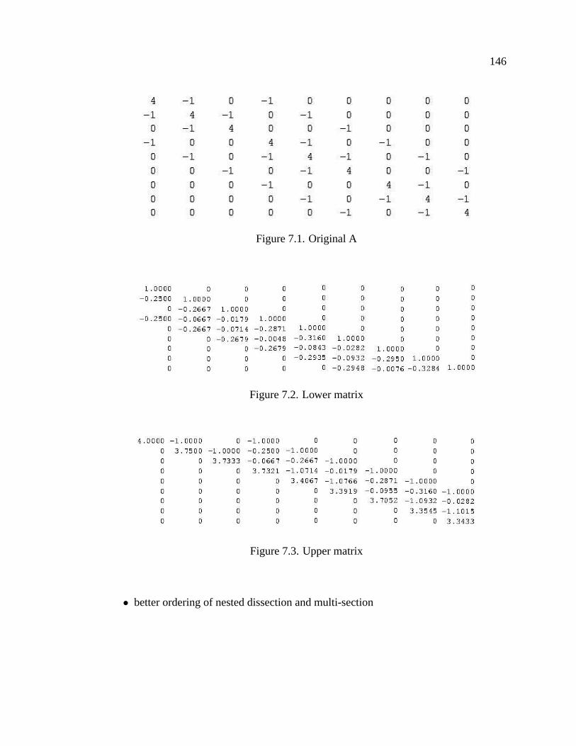
146
Figure 7.1. Original A
Figure 7.2. Lower matrix
Figure 7.3. Upper matrix
• better ordering of nested dissection and multi-section
147
7.2 Minimum Degree Ordering
The minimum degree ordering algorithm implemented in SPOOLES is described
in more detail in Liu [43]. One of the most widely used sparse matrix heuristic orderings
method before graph based ordering schemes, the minimum degree algorithm is loosely
similar to the algorithm proposed by Markowitz in 1957 and has proved very effective
in reducing computation time and fill-in [44]. When ordering sparse matrices, minimum
degree selects the vertex with the smallest degree and removes the vertex from the graph
by pivoting it, in essence makes the surrounding area of the vertex a clique, and then
moves on to the next vertex with the smallest degree in the graph [43]. By choosing
a vertex with minimum degree, the fill-in resulting from adding edges to the remaining
vertices is also at a minimum, than compared to a vertex with a higher degree [45].
These steps continue of selection and pivoting until all vertices have been elimi-
nated. The new elimination graph is formed by deleting the vertex of smallest degree and
its incident edges from the graph and then adding new edges so that the adjacent nodes of
the vertex are now pairwise adjacent [43]. These steps to forming the elimination graph
are illustrated in Figure 7.4 [41].
The minimum degree algorithm, however, is not without its drawbacks. One area of
trouble is that after a vertex has been eliminated and a new elimination graph is formed,
the degree of every vertex that has not been eliminated must be updated. This successive
new elimination tree creation and remaining vertices numbering update is the most time
consuming part in the ordering process [43]. The goal of multiple external minimum
degree introduced by Liu is to reduce the number of degree updates. Multiple elimina-
tion, as this modification is called, involves the elimination of multiple vertices with the
same current minimum degree before a complete update is performed [43]. The vertices
with the same current minimum degree form a set of independent nodes. The original
minimum degree algorithm has basically three steps in a main loop, Figure 7.5:
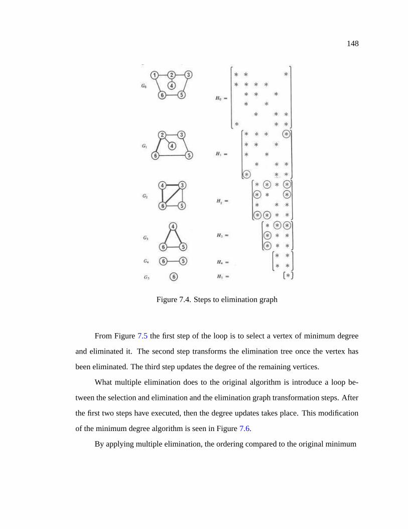
148
Figure 7.4. Steps to elimination graph
From Figure 7.5 the first step of the loop is to select a vertex of minimum degree
and eliminated it. The second step transforms the elimination tree once the vertex has
been eliminated. The third step updates the degree of the remaining vertices.
What multiple elimination does to the original algorithm is introduce a loop be-
tween the selection and elimination and the elimination graph transformation steps. After
the first two steps have executed, then the degree updates takes place. This modification
of the minimum degree algorithm is seen in Figure 7.6.
By applying multiple elimination, the ordering compared to the original minimum
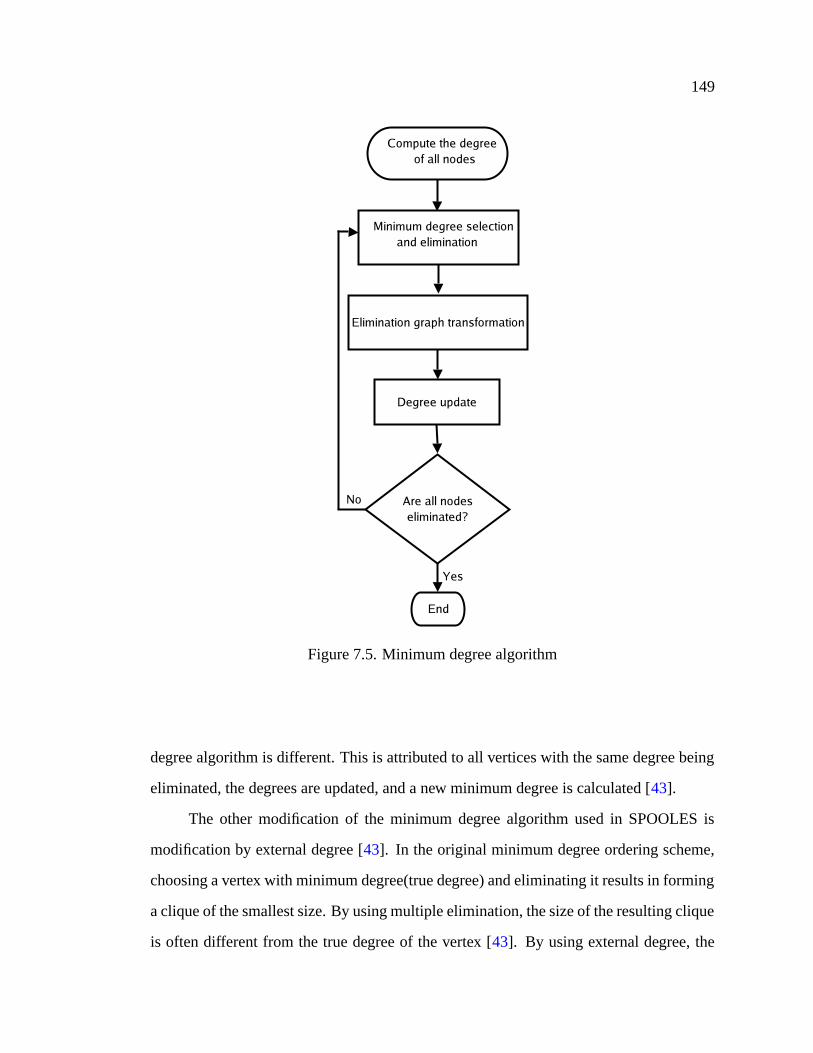
149
Figure 7.5. Minimum degree algorithm
degree algorithm is different. This is attributed to all vertices with the same degree being
eliminated, the degrees are updated, and a new minimum degree is calculated [43].
The other modification of the minimum degree algorithm used in SPOOLES is
modification by external degree [43]. In the original minimum degree ordering scheme,
choosing a vertex with minimum degree(true degree) and eliminating it results in forming
a clique of the smallest size. By using multiple elimination, the size of the resulting clique
is often different from the true degree of the vertex [43]. By using external degree, the
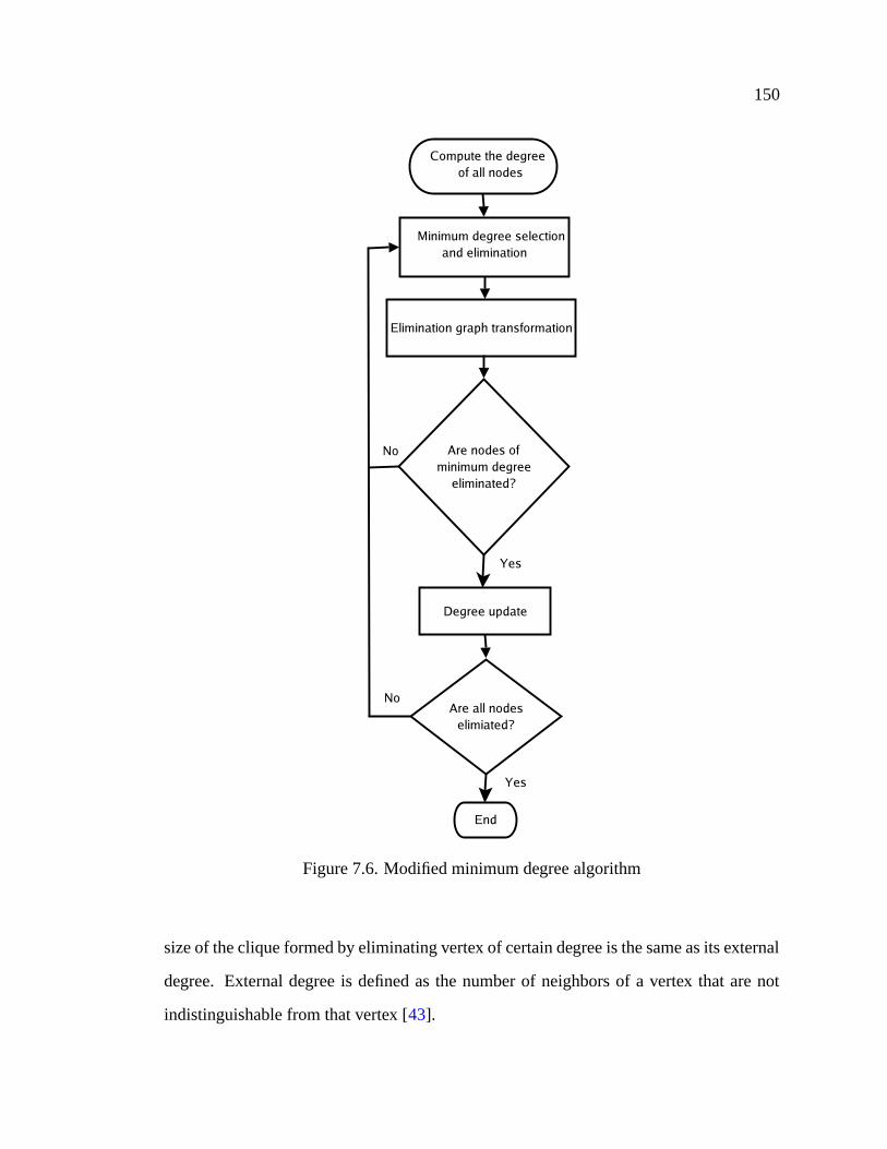
150
Figure 7.6. Modified minimum degree algorithm
size of the clique formed by eliminating vertex of certain degree is the same as its external
degree. External degree is defined as the number of neighbors of a vertex that are not
indistinguishable from that vertex [43].

151
The function call that is used for a multiple minimum degree ordering is the follow-
ing:
orderViaMMD(graph, seed, msglvl, msgFile);
7.3 Nested Dissection
Nested dissection [46] is considered a top down approach to matrix ordering. The
algorithm uses global information about the structure of the matrix, that is, it examines the
graph as a whole before ordering it. In comparison, minimum degree determines which
vertex should be eliminated first while nested dissection decides which vertices should be
eliminated last. The nested dissection algorithm begins by selecting a separator, a set of
vertices that partitions the graph into roughly equal parts. The vertices in the separator
are then labeled the highest and ordered last in the elimination sequence. The nested
dissection algorithm then continues the loop of finding a separator and ordering until the
entire graph has been ordered. By ordering the vertices in the separator last, the matrix
is permuted in a bordered block-diagonal structure. The zero off-diagonal blocks suffer
no fill-in during the factorization. By using a small separator, the size of the off-diagonal
blocks is maximized [45].
Another desirable attribute of a small separator is that typically the separator is a
clique. The properties of a clique limit the elimination of vertices to a sequential oper-
ation, not parallel, because within the clique, the vertices do not form independent sets.
Because they are dependent sets within a clique, the vertices can not be split up between
more than one processor.
The function call to use nested dissection for an ordering is:
orderViaND(graph, maxdomainsize, seed, msglvl, msgFile);
Maxdomainsize specifies the largest number of vertices allowed in a subgraph be-
fore it is split.
152
7.4 Multi-section
The multi-section ordering algorithm uses a multi-sector, a subset of vertices, that
divides the graph into two or more subgraphs [47]. Ordering my multi-section can be
compared to an incomplete nested dissection ordering. The graphs are split into sub-
graphs, subgraphs become graphs and then are split into more subgraphs. This continues
until the subgraphs reach some defined size. The user defined subgraph size is critical
for the performance of SPOOLES. This variable will be discussed in more detail in later
sections.
The use of multi-section is closely related to domain decomposition. The domain
decomposition step of multi-section occurs in three steps:
• Find an initial domain decomposition of the graph
• Find an initial separator formed of Multisection vertices
• Improve the bisector
All vertices in the domains are ordered before the vertices in the multi-sector. Do-
mains are independent of each other and, therefore, can be ordered independently. As
in the nested dissection ordering algorithm, after the graph is subdivided, the minimum
degree algorithm is then used to order the subgraphs [47].
The results presented in [47] on the testing of multi-section versus nested dissection
and multiple minimum degree show that multi-section is very competitive with the well
known partitioning tool METIS [48]. Several Harwell-Boeing [49] matrices were used
and the results show that multi-section performs as well as or better than multi-section
and nested dissection or many of the cases [47].
The function call to use multi-section is:
orderViaMS(graph, maxdomainsize, seed, msglvl, msgFile);
CHAPTER 8OPTIMIZING SPOOLES FOR A COW
This chapter will discuss the steps taken to optimize SPOOLES for our Cluster of
Workstations. The parallel functions of SPOOLES were originally coded for Massively
Parallel Processing machines that have a high-speed low-latency proprietary intercon-
nect. By optimizing certain parameters, SPOOLES will be tailored and optimized for our
network which is non-proprietary 100 Mbps Ethernet.
8.1 Installation
To use the parallel functions of SPOOLES, the parallel MPI library, spoolesMPI.a,
needs to be built. First, download SPOOLES from the website at [33]. Download the file
spooles.2.2.tgz, place it in the folder SPOOLES.2.2, and unpack.
redboots@apollo> cd /home/apollo/hda8
redboots@apollo> mkdir SPOOLES.2.2
redboots@apollo> mv spooles.2.2.tgz SPOOLES.2.2
redboots@apollo> cd SPOOLES.2.2
redboots@apollo> tar -xvzf spooles.2.2.tgz
This will unpack spooles.2.2.tgz in the folder SPOOLES.2.2. First, edit the file
Make.inc so that it points to the correct compiler, MPICH install location, MPICH li-
braries, and include directory.
CC = mpicc
MPI_INSTALL_DIR = /home/apollo/hda8/mpich-1.2.5.2
MPI_LIB_PATH = -L$(MPI_INSTALL_DIR)/lib
MPI_INCLUDE_DIR = -I$(MPI_INSTALL_DIR)/include
153
154
To create the parallel library, enter into the directory
/home/apollo/hda8/SPOOLES.2.2/MPI and type:
make lib
This will create the library spoolesMPI.a in /home/apollo/hda8/SPOOLES.2.2/
MPI/src. When p solver is compiled, the Makefile links to the parallel library, spoolesMPI.a.
P solver is the parallel solver that utilizes the parallel routines of SPOOLES. The
source code and binary executable p solver are located in
/home/apollo/hda8/CalculiX/ccx 1.1/src/p solver. The source code and Makefile used
to compile p solver are shown in Appendix E.2.1 and E.2.2 respectively. To compile
p solver, type:
redboots@apollo> make
mpicc -O -I ../../../../SPOOLES.2.2 -DARCH="Linux" -c
-o p_solver.o p_solver.c mpicc p_solver.o -o p_solver
/home/apollo/hda8/SPOOLES.2.2/MPI/src/spoolesMPI.a
/home/apollo/hda8/SPOOLES.2.2/spooles.a -lm -lpthread
p solver is a separate program from ccx. For the tests performed during the opti-
mization process, p solver is run by invoking a call to mpirun. For a two processor test,
the following command is used.
redboots@apollo> mpirun -np 2 p_solver
8.2 Optimization
The test case that will be used for the optimization is a cantilever beam, ten inches
long, a 1x1 inch cross-section, with a 200lb load applied to the end, Figure 8.1. The
material is AISI 1018 Steel.
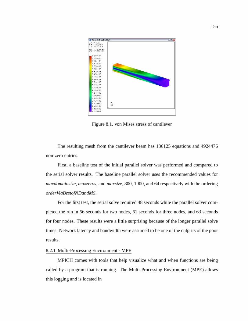
155
Figure 8.1. von Mises stress of cantilever
The resulting mesh from the cantilever beam has 136125 equations and 4924476
non-zero entries.
First, a baseline test of the initial parallel solver was performed and compared to
the serial solver results. The baseline parallel solver uses the recommended values for
maxdomainsize, maxzeros, and maxsize, 800, 1000, and 64 respectively with the ordering
orderViaBestofNDandMS.
For the first test, the serial solve required 48 seconds while the parallel solver com-
pleted the run in 56 seconds for two nodes, 61 seconds for three nodes, and 63 seconds
for four nodes. These results were a little surprising because of the longer parallel solve
times. Network latency and bandwidth were assumed to be one of the culprits of the poor
results.
8.2.1 Multi-Processing Environment - MPE
MPICH comes with tools that help visualize what and when functions are being
called by a program that is running. The Multi-Processing Environment (MPE) allows
this logging and is located in
156
/home/apollo/hda8/mpich-1.2.5.2/mpe. MPE provides performance analysis tools for MPI
programs through a post-processing approach. Provided are the necessary libraries to link
against and a log viewer, upshot. Upshot reads the log files and presents a graphical view
of the communication between nodes, what functions are called, and the time-frame in
which the functions are called. These tools will help determine what communication
occurs between nodes and help with the optimization process.
To enable logging, several options need to be added to the Makefile for p solver.
These are:
MPE_LIBDIR = /home/apollo/hda8/mpich-1.2.5.2/mpe/lib
LOG_LIBS = -L$(MPE_LIBDIR) -llmpe -lmpe
p_solver: p_solver.o
${CC} p_solver.o -o $@ ${LIBS} ${LOG_LIBS}
When p solver is now run, it will create a log-file named p solver.clog. Convert the
*.clog file to the format for upshot, *.alog, and then run upshot. The below example is a
small test problem with 5400 equations and 173196 non-zero entries.
redboots@apollo > /home/apollo/hda8/mpich-1.2.5.2/mpe/ \
bin/clog2alog p_solver
redboots@apollo > /home/apollo/hda8/mpich-1.2.5.2/mpe/ \
viewers/upshot/bin/upshot p_solver.alog
First, p solver was run just using two processors. The resulting log for a small test
problem is shown in Figure 8.2.
At the top of the screen the MPI routines are color-coded. The black arrows repre-
sent communication between nodes. On the right hand side it can be seen that there is a
lot of communication occurring between the two nodes. Each communication has inher-
ent latency induced by the network. Viewing a zoomed portion of the log file shows that
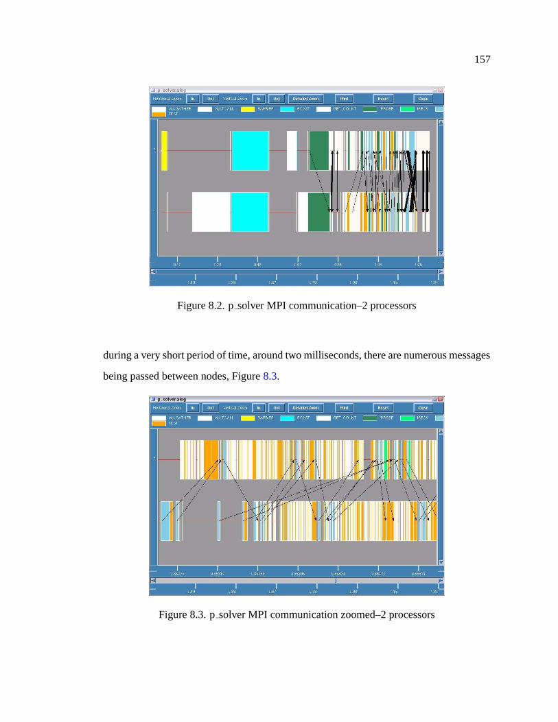
157
Figure 8.2. p solver MPI communication–2 processors
during a very short period of time, around two milliseconds, there are numerous messages
being passed between nodes, Figure 8.3.
Figure 8.3. p solver MPI communication zoomed–2 processors
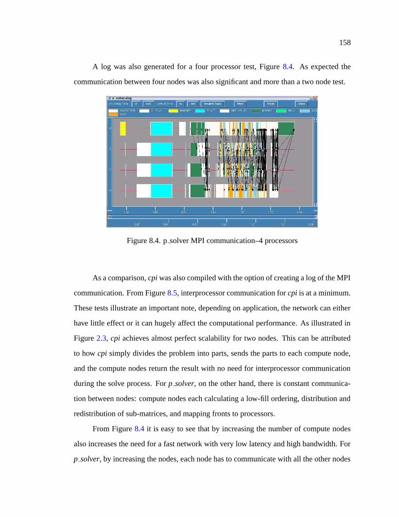
158
A log was also generated for a four processor test, Figure 8.4. As expected the
communication between four nodes was also significant and more than a two node test.
Figure 8.4. p solver MPI communication–4 processors
As a comparison, cpi was also compiled with the option of creating a log of the MPI
communication. From Figure 8.5, interprocessor communication for cpi is at a minimum.
These tests illustrate an important note, depending on application, the network can either
have little effect or it can hugely affect the computational performance. As illustrated in
Figure 2.3, cpi achieves almost perfect scalability for two nodes. This can be attributed
to how cpi simply divides the problem into parts, sends the parts to each compute node,
and the compute nodes return the result with no need for interprocessor communication
during the solve process. For p solver, on the other hand, there is constant communica-
tion between nodes: compute nodes each calculating a low-fill ordering, distribution and
redistribution of sub-matrices, and mapping fronts to processors.
From Figure 8.4 it is easy to see that by increasing the number of compute nodes
also increases the need for a fast network with very low latency and high bandwidth. For
p solver, by increasing the nodes, each node has to communicate with all the other nodes
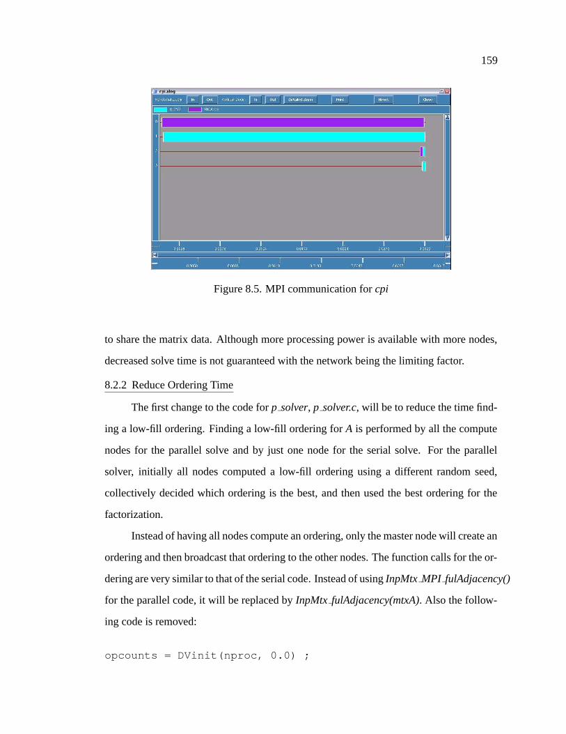
159
Figure 8.5. MPI communication for cpi
to share the matrix data. Although more processing power is available with more nodes,
decreased solve time is not guaranteed with the network being the limiting factor.
8.2.2 Reduce Ordering Time
The first change to the code for p solver, p solver.c, will be to reduce the time find-
ing a low-fill ordering. Finding a low-fill ordering for A is performed by all the compute
nodes for the parallel solve and by just one node for the serial solve. For the parallel
solver, initially all nodes computed a low-fill ordering using a different random seed,
collectively decided which ordering is the best, and then used the best ordering for the
factorization.
Instead of having all nodes compute an ordering, only the master node will create an
ordering and then broadcast that ordering to the other nodes. The function calls for the or-
dering are very similar to that of the serial code. Instead of using InpMtx MPI fulAdjacency()
for the parallel code, it will be replaced by InpMtx fulAdjacency(mtxA). Also the follow-
ing code is removed:
opcounts = DVinit(nproc, 0.0) ;
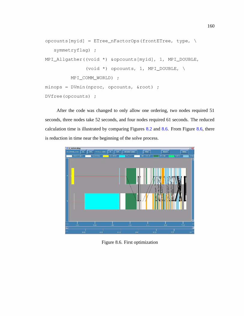
160
opcounts[myid] = ETree_nFactorOps(frontETree, type, \
symmetryflag) ;
MPI_Allgather((void *) &opcounts[myid], 1, MPI_DOUBLE,
(void *) opcounts, 1, MPI_DOUBLE, \
MPI_COMM_WORLD) ;
minops = DVmin(nproc, opcounts, &root) ;
DVfree(opcounts) ;
After the code was changed to only allow one ordering, two nodes required 51
seconds, three nodes take 52 seconds, and four nodes required 61 seconds. The reduced
calculation time is illustrated by comparing Figures 8.2 and 8.6. From Figure 8.6, there
is reduction in time near the beginning of the solve process.
Figure 8.6. First optimization
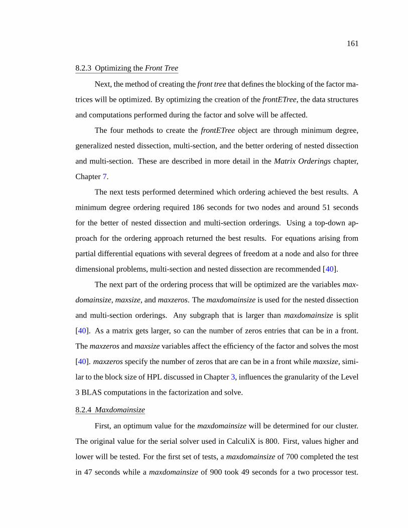
161
8.2.3 Optimizing the Front Tree
Next, the method of creating the front tree that defines the blocking of the factor ma-
trices will be optimized. By optimizing the creation of the frontETree, the data structures
and computations performed during the factor and solve will be affected.
The four methods to create the frontETree object are through minimum degree,
generalized nested dissection, multi-section, and the better ordering of nested dissection
and multi-section. These are described in more detail in the Matrix Orderings chapter,
Chapter 7.
The next tests performed determined which ordering achieved the best results. A
minimum degree ordering required 186 seconds for two nodes and around 51 seconds
for the better of nested dissection and multi-section orderings. Using a top-down ap-
proach for the ordering approach returned the best results. For equations arising from
partial differential equations with several degrees of freedom at a node and also for three
dimensional problems, multi-section and nested dissection are recommended [40].
The next part of the ordering process that will be optimized are the variables max-
domainsize, maxsize, and maxzeros. The maxdomainsize is used for the nested dissection
and multi-section orderings. Any subgraph that is larger than maxdomainsize is split
[40]. As a matrix gets larger, so can the number of zeros entries that can be in a front.
The maxzeros and maxsize variables affect the efficiency of the factor and solves the most
[40]. maxzeros specify the number of zeros that are can be in a front while maxsize, simi-
lar to the block size of HPL discussed in Chapter 3, influences the granularity of the Level
3 BLAS computations in the factorization and solve.
8.2.4 Maxdomainsize
First, an optimum value for the maxdomainsize will be determined for our cluster.
The original value for the serial solver used in CalculiX is 800. First, values higher and
lower will be tested. For the first set of tests, a maxdomainsize of 700 completed the test
in 47 seconds while a maxdomainsize of 900 took 49 seconds for a two processor test.
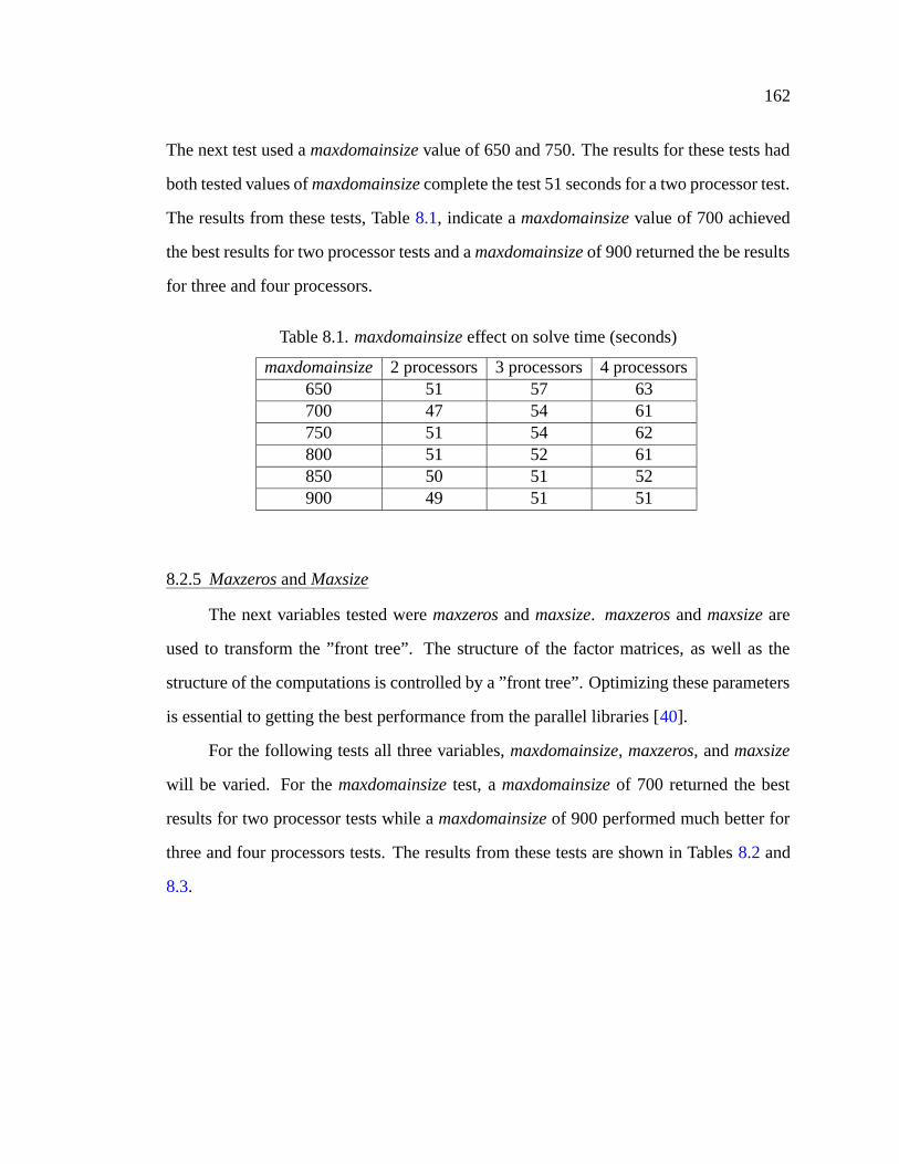
162
The next test used a maxdomainsize value of 650 and 750. The results for these tests had
both tested values of maxdomainsize complete the test 51 seconds for a two processor test.
The results from these tests, Table 8.1, indicate a maxdomainsize value of 700 achieved
the best results for two processor tests and a maxdomainsize of 900 returned the be results
for three and four processors.
Table 8.1. maxdomainsize effect on solve time (seconds)
maxdomainsize 2 processors 3 processors 4 processors650 51 57 63700 47 54 61750 51 54 62800 51 52 61850 50 51 52900 49 51 51
8.2.5 Maxzeros and Maxsize
The next variables tested were maxzeros and maxsize. maxzeros and maxsize are
used to transform the ”front tree”. The structure of the factor matrices, as well as the
structure of the computations is controlled by a ”front tree”. Optimizing these parameters
is essential to getting the best performance from the parallel libraries [40].
For the following tests all three variables, maxdomainsize, maxzeros, and maxsize
will be varied. For the maxdomainsize test, a maxdomainsize of 700 returned the best
results for two processor tests while a maxdomainsize of 900 performed much better for
three and four processors tests. The results from these tests are shown in Tables 8.2 and
8.3.
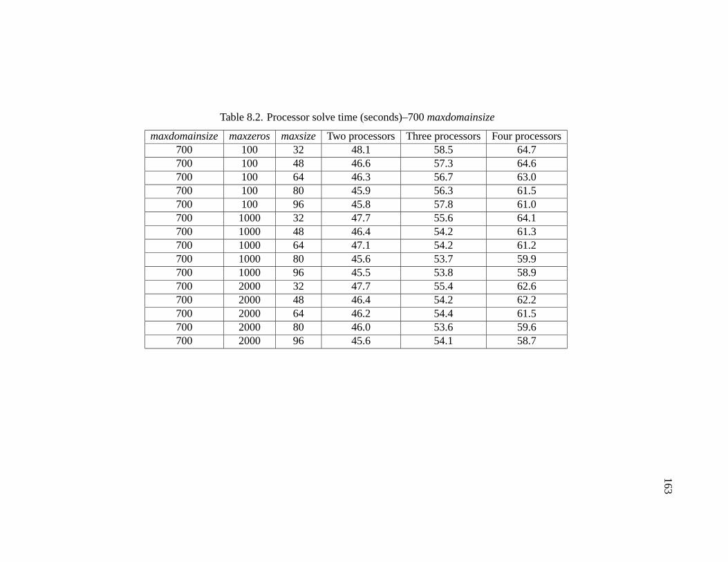
163
Table 8.2. Processor solve time (seconds)–700 maxdomainsize
maxdomainsize maxzeros maxsize Two processors Three processors Four processors700 100 32 48.1 58.5 64.7700 100 48 46.6 57.3 64.6700 100 64 46.3 56.7 63.0700 100 80 45.9 56.3 61.5700 100 96 45.8 57.8 61.0700 1000 32 47.7 55.6 64.1700 1000 48 46.4 54.2 61.3700 1000 64 47.1 54.2 61.2700 1000 80 45.6 53.7 59.9700 1000 96 45.5 53.8 58.9700 2000 32 47.7 55.4 62.6700 2000 48 46.4 54.2 62.2700 2000 64 46.2 54.4 61.5700 2000 80 46.0 53.6 59.6700 2000 96 45.6 54.1 58.7
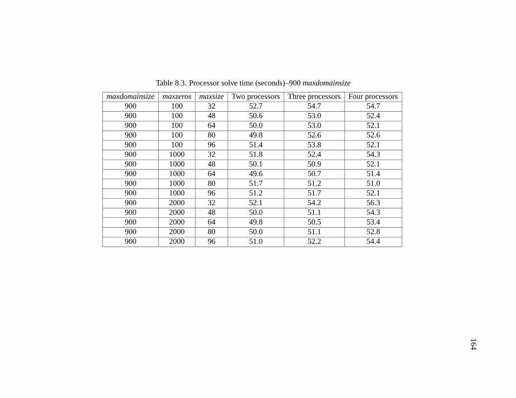
164
Table 8.3. Processor solve time (seconds)–900 maxdomainsize
maxdomainsize maxzeros maxsize Two processors Three processors Four processors900 100 32 52.7 54.7 54.7900 100 48 50.6 53.0 52.4900 100 64 50.0 53.0 52.1900 100 80 49.8 52.6 52.6900 100 96 51.4 53.8 52.1900 1000 32 51.8 52.4 54.3900 1000 48 50.1 50.9 52.1900 1000 64 49.6 50.7 51.4900 1000 80 51.7 51.2 51.0900 1000 96 51.2 51.7 52.1900 2000 32 52.1 54.2 56.3900 2000 48 50.0 51.1 54.3900 2000 64 49.8 50.5 53.4900 2000 80 50.0 51.1 52.8900 2000 96 51.0 52.2 54.4
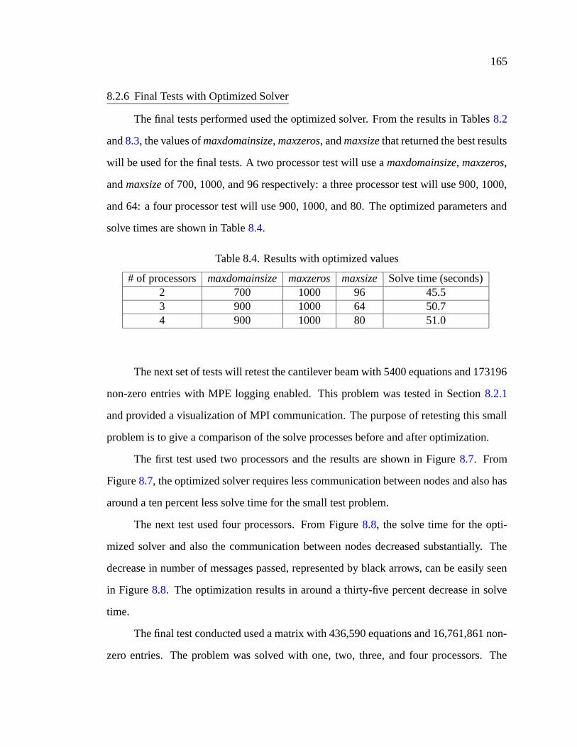
165
8.2.6 Final Tests with Optimized Solver
The final tests performed used the optimized solver. From the results in Tables 8.2
and 8.3, the values of maxdomainsize, maxzeros, and maxsize that returned the best results
will be used for the final tests. A two processor test will use a maxdomainsize, maxzeros,
and maxsize of 700, 1000, and 96 respectively: a three processor test will use 900, 1000,
and 64: a four processor test will use 900, 1000, and 80. The optimized parameters and
solve times are shown in Table 8.4.
Table 8.4. Results with optimized values
# of processors maxdomainsize maxzeros maxsize Solve time (seconds)2 700 1000 96 45.53 900 1000 64 50.74 900 1000 80 51.0
The next set of tests will retest the cantilever beam with 5400 equations and 173196
non-zero entries with MPE logging enabled. This problem was tested in Section 8.2.1
and provided a visualization of MPI communication. The purpose of retesting this small
problem is to give a comparison of the solve processes before and after optimization.
The first test used two processors and the results are shown in Figure 8.7. From
Figure 8.7, the optimized solver requires less communication between nodes and also has
around a ten percent less solve time for the small test problem.
The next test used four processors. From Figure 8.8, the solve time for the opti-
mized solver and also the communication between nodes decreased substantially. The
decrease in number of messages passed, represented by black arrows, can be easily seen
in Figure 8.8. The optimization results in around a thirty-five percent decrease in solve
time.
The final test conducted used a matrix with 436,590 equations and 16,761,861 non-
zero entries. The problem was solved with one, two, three, and four processors. The
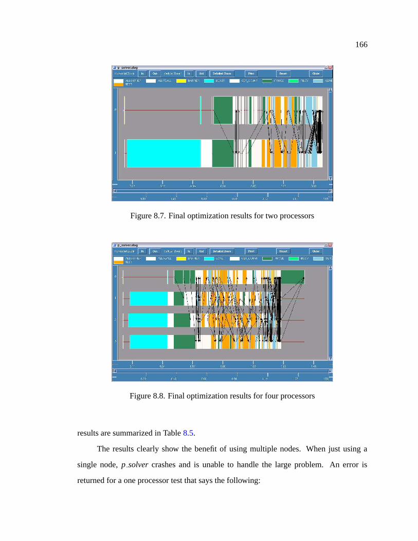
166
Figure 8.7. Final optimization results for two processors
Figure 8.8. Final optimization results for four processors
results are summarized in Table 8.5.
The results clearly show the benefit of using multiple nodes. When just using a
single node, p solver crashes and is unable to handle the large problem. An error is
returned for a one processor test that says the following:
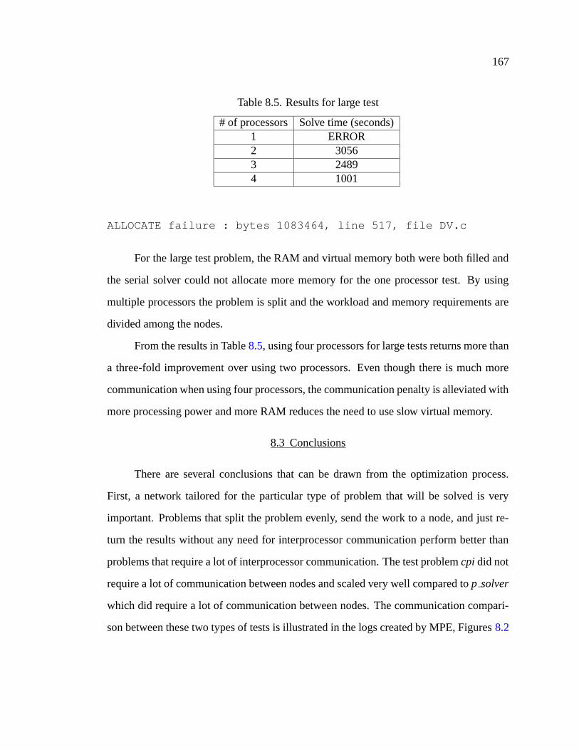
167
Table 8.5. Results for large test
# of processors Solve time (seconds)1 ERROR2 30563 24894 1001
ALLOCATE failure : bytes 1083464, line 517, file DV.c
For the large test problem, the RAM and virtual memory both were both filled and
the serial solver could not allocate more memory for the one processor test. By using
multiple processors the problem is split and the workload and memory requirements are
divided among the nodes.
From the results in Table 8.5, using four processors for large tests returns more than
a three-fold improvement over using two processors. Even though there is much more
communication when using four processors, the communication penalty is alleviated with
more processing power and more RAM reduces the need to use slow virtual memory.
8.3 Conclusions
There are several conclusions that can be drawn from the optimization process.
First, a network tailored for the particular type of problem that will be solved is very
important. Problems that split the problem evenly, send the work to a node, and just re-
turn the results without any need for interprocessor communication perform better than
problems that require a lot of interprocessor communication. The test problem cpi did not
require a lot of communication between nodes and scaled very well compared to p solver
which did require a lot of communication between nodes. The communication compari-
son between these two types of tests is illustrated in the logs created by MPE, Figures 8.2
168
and 8.5. A 100 Mbps Ethernet network is sufficient for a problem such as cpi but with
problems that require heavy communication, high bandwidth and low latency network
hardware such as Myrinet [21] is essential for the performance to scale well and to achieve
acceptable solve times.
The performance of a cluster is also very dependent on well written software that
is optimized for the available network and computer hardware. This is well illustrated
in the optimization process for p solver. For the small test problem, around a ten per-
cent performance gain for a two processor system and around a thirty-five performance
increase for four nodes was achieved by optimizing p solver for our network and com-
puter architecture. By optimizing the granularity of the Level 3 BLAS computations in
the factorization and solve process by changing the maxsize parameter, the performance
of p solver is greatly increased. Although a maxsize of 64 is the recommended value for
most systems, primarily MPP’s, by changing the maxsize value to 96 for two processors
and to 80 for four processors, p solver becomes tailored for our system. Although settings
and program coding may be optimized for one architecture, this does not guarantee that
the program will be optimized and perform well for another system.
8.3.1 Recommendations
In order to achieve better performance from our cluster, more RAM and a faster
network should be purchased. Unlike an iterative system of equations solver, a direct
solver stores the entire problem in RAM. When the RAM is filled, slow virtual memory
is then used. By increasing the RAM, more of the problem can be stored in the RAM
and decrease the dependence on the hard disk. From Table 8.4, the increased available
RAM from using four processors disproportionately outperforms using just half of the
processors. With more RAM for each node, increased performance should be expected.
The network on which our cluster communicates should also be upgraded. For
problems that do not require alot of communication such as cpi, a 100 Mbps Ethernet is
sufficient. Because of the heavy communication in solving systems of equations, a high
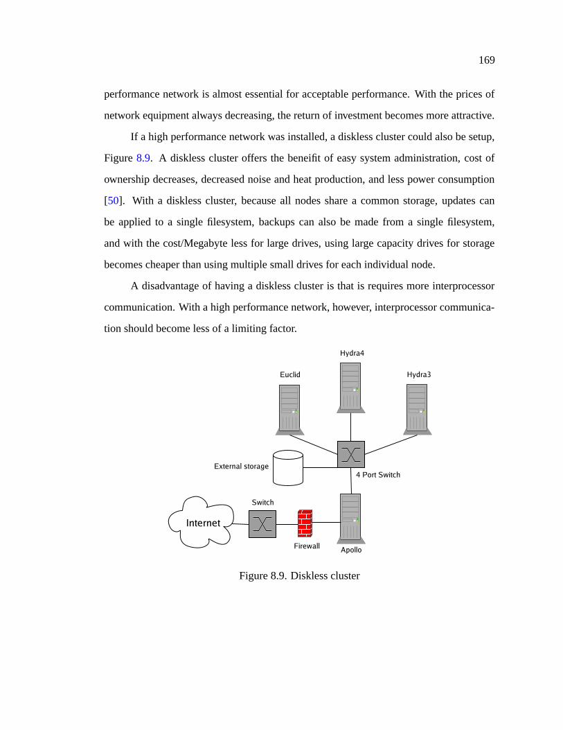
169
performance network is almost essential for acceptable performance. With the prices of
network equipment always decreasing, the return of investment becomes more attractive.
If a high performance network was installed, a diskless cluster could also be setup,
Figure 8.9. A diskless cluster offers the beneifit of easy system administration, cost of
ownership decreases, decreased noise and heat production, and less power consumption
[50]. With a diskless cluster, because all nodes share a common storage, updates can
be applied to a single filesystem, backups can also be made from a single filesystem,
and with the cost/Megabyte less for large drives, using large capacity drives for storage
becomes cheaper than using multiple small drives for each individual node.
A disadvantage of having a diskless cluster is that is requires more interprocessor
communication. With a high performance network, however, interprocessor communica-
tion should become less of a limiting factor.
Figure 8.9. Diskless cluster
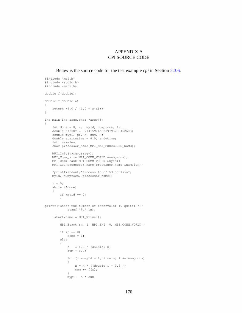
APPENDIX ACPI SOURCE CODE
Below is the source code for the test example cpi in Section 2.3.6.
#include "mpi.h"#include <stdio.h>#include <math.h>
double f(double);
double f(double a){
return (4.0 / (1.0 + a*a));}
int main(int argc,char *argv[]){
int done = 0, n, myid, numprocs, i;double PI25DT = 3.141592653589793238462643;double mypi, pi, h, sum, x;double startwtime = 0.0, endwtime;int namelen;char processor_name[MPI_MAX_PROCESSOR_NAME];
MPI_Init(&argc,&argv);MPI_Comm_size(MPI_COMM_WORLD,&numprocs);MPI_Comm_rank(MPI_COMM_WORLD,&myid);MPI_Get_processor_name(processor_name,&namelen);
fprintf(stdout,"Process %d of %d on %s\n",myid, numprocs, processor_name);
n = 0;while (!done){
if (myid == 0){
printf("Enter the number of intervals: (0 quits) ");scanf("%d",&n);
startwtime = MPI_Wtime();}MPI_Bcast(&n, 1, MPI_INT, 0, MPI_COMM_WORLD);
if (n == 0)done = 1;
else{
h = 1.0 / (double) n;sum = 0.0;
for (i = myid + 1; i <= n; i += numprocs){
x = h * ((double)i - 0.5 );sum += f(x);
}mypi = h * sum;
170
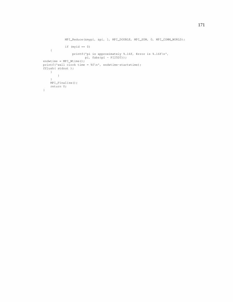
171
MPI_Reduce(&mypi, &pi, 1, MPI_DOUBLE, MPI_SUM, 0, MPI_COMM_WORLD);
if (myid == 0){
printf("pi is approximately %.16f, Error is %.16f\n",pi, fabs(pi - PI25DT));
endwtime = MPI_Wtime();printf("wall clock time = %f\n", endwtime-startwtime);fflush( stdout );
}}
}MPI_Finalize();return 0;
}
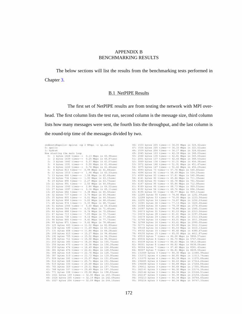
APPENDIX BBENCHMARKING RESULTS
The below sections will list the results from the benchmarking tests performed in
Chapter 3.
B.1 NetPIPE Results
The first set of NetPIPE results are from testing the network with MPI over-
head. The first column lists the test run, second column is the message size, third column
lists how many messages were sent, the fourth lists the throughput, and the last column is
the round-trip time of the messages divided by two.
redboots@apollo> mpirun -np 2 NPmpi -o np.out.mpi0: apollo1: hydra4Now starting the main loop0: 1 bytes 1628 times--> 0.13 Mbps in 60.98usec1: 2 bytes 1639 times--> 0.25 Mbps in 60.87usec2: 3 bytes 1642 times--> 0.37 Mbps in 61.07usec3: 4 bytes 1091 times--> 0.50 Mbps in 61.46usec4: 6 bytes 1220 times--> 0.74 Mbps in 61.48usec5: 8 bytes 813 times--> 0.99 Mbps in 61.86usec6: 12 bytes 1010 times--> 1.46 Mbps in 62.53usec7: 13 bytes 666 times--> 1.58 Mbps in 62.66usec8: 16 bytes 736 times--> 1.93 Mbps in 63.15usec9: 19 bytes 890 times--> 2.27 Mbps in 63.73usec10: 21 bytes 991 times--> 2.50 Mbps in 64.09usec11: 24 bytes 1040 times--> 2.84 Mbps in 64.52usec12: 27 bytes 1097 times--> 3.16 Mbps in 65.11usec13: 29 bytes 682 times--> 3.38 Mbps in 65.50usec14: 32 bytes 737 times--> 3.70 Mbps in 65.94usec15: 35 bytes 805 times--> 4.01 Mbps in 66.56usec16: 45 bytes 858 times--> 5.02 Mbps in 68.43usec17: 48 bytes 974 times--> 5.33 Mbps in 68.72usec18: 51 bytes 1000 times--> 5.60 Mbps in 69.43usec19: 61 bytes 564 times--> 6.52 Mbps in 71.40usec20: 64 bytes 688 times--> 6.76 Mbps in 72.28usec21: 67 bytes 713 times--> 7.03 Mbps in 72.72usec22: 93 bytes 738 times--> 9.16 Mbps in 77.46usec23: 96 bytes 860 times--> 9.42 Mbps in 77.73usec24: 99 bytes 871 times--> 9.62 Mbps in 78.48usec25: 125 bytes 463 times--> 11.52 Mbps in 82.80usec26: 128 bytes 599 times--> 11.69 Mbps in 83.51usec27: 131 bytes 608 times--> 11.86 Mbps in 84.28usec28: 189 bytes 615 times--> 15.27 Mbps in 94.46usec29: 192 bytes 705 times--> 15.52 Mbps in 94.39usec30: 195 bytes 711 times--> 15.58 Mbps in 95.50usec31: 253 bytes 365 times--> 18.25 Mbps in 105.75usec32: 256 bytes 470 times--> 18.38 Mbps in 106.28usec33: 259 bytes 474 times--> 18.49 Mbps in 106.88usec34: 381 bytes 476 times--> 22.61 Mbps in 128.59usec35: 384 bytes 518 times--> 22.76 Mbps in 128.75usec36: 387 bytes 519 times--> 22.73 Mbps in 129.90usec37: 509 bytes 262 times--> 25.57 Mbps in 151.85usec38: 512 bytes 328 times--> 25.71 Mbps in 151.94usec39: 515 bytes 330 times--> 25.68 Mbps in 153.02usec40: 765 bytes 329 times--> 29.51 Mbps in 197.76usec41: 768 bytes 337 times--> 29.69 Mbps in 197.34usec42: 771 bytes 338 times--> 29.58 Mbps in 198.83usec43: 1021 bytes 169 times--> 32.00 Mbps in 243.39usec44: 1024 bytes 205 times--> 32.19 Mbps in 242.69usec45: 1027 bytes 206 times--> 32.09 Mbps in 244.15usec
46: 1533 bytes 205 times--> 36.05 Mbps in 324.42usec47: 1536 bytes 205 times--> 36.33 Mbps in 322.52usec48: 1539 bytes 206 times--> 36.17 Mbps in 324.62usec49: 2045 bytes 103 times--> 42.39 Mbps in 368.03usec50: 2048 bytes 135 times--> 42.81 Mbps in 365.00usec51: 2051 bytes 137 times--> 42.46 Mbps in 368.53usec52: 3069 bytes 136 times--> 51.31 Mbps in 456.36usec53: 3072 bytes 146 times--> 51.91 Mbps in 451.47usec54: 3075 bytes 147 times--> 51.42 Mbps in 456.29usec55: 4093 bytes 73 times--> 57.76 Mbps in 540.60usec56: 4096 bytes 92 times--> 58.49 Mbps in 534.29usec57: 4099 bytes 93 times--> 57.81 Mbps in 540.98usec58: 6141 bytes 92 times--> 65.86 Mbps in 711.39usec59: 6144 bytes 93 times--> 66.78 Mbps in 701.92usec60: 6147 bytes 95 times--> 65.86 Mbps in 712.08usec61: 8189 bytes 46 times--> 68.73 Mbps in 909.03usec62: 8192 bytes 54 times--> 69.74 Mbps in 896.18usec63: 8195 bytes 55 times--> 68.77 Mbps in 909.13usec64: 12285 bytes 55 times--> 74.86 Mbps in 1251.99usec65: 12288 bytes 53 times--> 76.00 Mbps in 1233.56usec66: 12291 bytes 54 times--> 74.87 Mbps in 1252.53usec67: 16381 bytes 26 times--> 77.13 Mbps in 1620.44usec68: 16384 bytes 30 times--> 79.39 Mbps in 1574.45usec69: 16387 bytes 31 times--> 78.86 Mbps in 1585.31usec70: 24573 bytes 31 times--> 81.03 Mbps in 2313.56usec71: 24576 bytes 28 times--> 81.61 Mbps in 2297.59usec72: 24579 bytes 29 times--> 81.05 Mbps in 2313.69usec73: 32765 bytes 14 times--> 83.01 Mbps in 3011.39usec74: 32768 bytes 16 times--> 83.61 Mbps in 2990.00usec75: 32771 bytes 16 times--> 83.00 Mbps in 3012.31usec76: 49149 bytes 16 times--> 85.03 Mbps in 4410.13usec77: 49152 bytes 15 times--> 85.60 Mbps in 4380.67usec78: 49155 bytes 15 times--> 85.00 Mbps in 4411.87usec79: 65533 bytes 7 times--> 86.08 Mbps in 5808.57usec80: 65536 bytes 8 times--> 86.70 Mbps in 5767.06usec81: 65539 bytes 8 times--> 86.02 Mbps in 5812.68usec82: 98301 bytes 8 times--> 86.82 Mbps in 8638.06usec83: 98304 bytes 7 times--> 87.40 Mbps in 8581.43usec84: 98307 bytes 7 times--> 86.81 Mbps in 8639.50usec85: 131069 bytes 3 times--> 86.30 Mbps in 11586.99usec86: 131072 bytes 4 times--> 86.85 Mbps in 11513.74usec87: 131075 bytes 4 times--> 86.39 Mbps in 11575.89usec88: 196605 bytes 4 times--> 86.63 Mbps in 17314.26usec89: 196608 bytes 3 times--> 86.88 Mbps in 17264.84usec90: 196611 bytes 3 times--> 86.68 Mbps in 17305.98usec91: 262141 bytes 3 times--> 86.30 Mbps in 23174.34usec92: 262144 bytes 3 times--> 86.34 Mbps in 23164.51usec93: 262147 bytes 3 times--> 86.38 Mbps in 23154.16usec94: 393213 bytes 3 times--> 86.34 Mbps in 34744.65usec95: 393216 bytes 3 times--> 86.34 Mbps in 34747.33usec
172
173
96: 393219 bytes 3 times--> 86.37 Mbps in 34735.02usec97: 524285 bytes 3 times--> 86.61 Mbps in 46183.49usec98: 524288 bytes 3 times--> 86.58 Mbps in 46199.16usec99: 524291 bytes 3 times--> 86.61 Mbps in 46182.65usec
100: 786429 bytes 3 times--> 86.88 Mbps in 69064.00usec101: 786432 bytes 3 times--> 86.84 Mbps in 69089.16usec102: 786435 bytes 3 times--> 86.92 Mbps in 69027.50usec103: 1048573 bytes 3 times--> 87.04 Mbps in 91907.51usec104: 1048576 bytes 3 times--> 87.00 Mbps in 91949.85usec105: 1048579 bytes 3 times--> 86.96 Mbps in 91994.35usec106: 1572861 bytes 3 times--> 87.01 Mbps in 137916.65usec107: 1572864 bytes 3 times--> 87.00 Mbps in 137927.82usec108: 1572867 bytes 3 times--> 87.11 Mbps in 137763.49usec109: 2097149 bytes 3 times--> 87.09 Mbps in 183727.48usec110: 2097152 bytes 3 times--> 87.04 Mbps in 183826.49usec
111: 2097155 bytes 3 times--> 87.19 Mbps in 183506.19usec112: 3145725 bytes 3 times--> 87.14 Mbps in 275412.17usec113: 3145728 bytes 3 times--> 87.14 Mbps in 275419.01usec114: 3145731 bytes 3 times--> 87.26 Mbps in 275046.49usec115: 4194301 bytes 3 times--> 87.18 Mbps in 367065.66usec116: 4194304 bytes 3 times--> 87.16 Mbps in 367126.34usec117: 4194307 bytes 3 times--> 87.30 Mbps in 366560.66usec118: 6291453 bytes 3 times--> 87.24 Mbps in 550221.68usec119: 6291456 bytes 3 times--> 87.21 Mbps in 550399.18usec120: 6291459 bytes 3 times--> 87.35 Mbps in 549535.67usec121: 8388605 bytes 3 times--> 87.32 Mbps in 732942.65usec122: 8388608 bytes 3 times--> 87.29 Mbps in 733149.68usec123: 8388611 bytes 3 times--> 87.37 Mbps in 732529.83usec
B.2 NetPIPE TCP Results
The below results are for testing the network with just TCP overhead; the
MPI overhead has been removed. The steps to performing this test is found in Section
3.2.3.
Send and receive buffers are 16384 and 87380 bytes(A bug in Linux doubles the requested buffer sizes)Now starting the main loop0: 1 bytes 2454 times--> 0.19 Mbps in 40.45usec1: 2 bytes 2472 times--> 0.38 Mbps in 40.02usec2: 3 bytes 2499 times--> 0.57 Mbps in 40.50usec3: 4 bytes 1645 times--> 0.75 Mbps in 40.51usec4: 6 bytes 1851 times--> 1.12 Mbps in 41.03usec5: 8 bytes 1218 times--> 1.47 Mbps in 41.64usec6: 12 bytes 1500 times--> 2.18 Mbps in 42.05usec7: 13 bytes 990 times--> 2.33 Mbps in 42.54usec8: 16 bytes 1084 times--> 2.86 Mbps in 42.64usec9: 19 bytes 1319 times--> 3.34 Mbps in 43.36usec10: 21 bytes 1456 times--> 3.67 Mbps in 43.67usec11: 24 bytes 1526 times--> 4.15 Mbps in 44.12usec12: 27 bytes 1605 times--> 4.61 Mbps in 44.65usec13: 29 bytes 995 times--> 4.90 Mbps in 45.14usec14: 32 bytes 1069 times--> 5.35 Mbps in 45.60usec15: 35 bytes 1165 times--> 5.77 Mbps in 46.28usec16: 45 bytes 1234 times--> 7.11 Mbps in 48.30usec17: 48 bytes 1380 times--> 7.56 Mbps in 48.43usec18: 51 bytes 1419 times--> 7.93 Mbps in 49.05usec19: 61 bytes 799 times--> 9.11 Mbps in 51.07usec20: 64 bytes 963 times--> 9.47 Mbps in 51.54usec21: 67 bytes 1000 times--> 9.79 Mbps in 52.21usec22: 93 bytes 1029 times--> 12.44 Mbps in 57.02usec23: 96 bytes 1169 times--> 12.79 Mbps in 57.28usec24: 99 bytes 1182 times--> 13.04 Mbps in 57.92usec25: 125 bytes 627 times--> 15.22 Mbps in 62.64usec26: 128 bytes 791 times--> 15.41 Mbps in 63.36usec27: 131 bytes 801 times--> 15.60 Mbps in 64.06usec28: 189 bytes 810 times--> 19.22 Mbps in 75.01usec29: 192 bytes 888 times--> 19.38 Mbps in 75.58usec30: 195 bytes 889 times--> 19.38 Mbps in 76.77usec31: 253 bytes 454 times--> 22.33 Mbps in 86.46usec32: 256 bytes 576 times--> 22.52 Mbps in 86.73usec33: 259 bytes 581 times--> 22.60 Mbps in 87.42usec34: 381 bytes 582 times--> 26.75 Mbps in 108.65usec35: 384 bytes 613 times--> 26.76 Mbps in 109.46usec36: 387 bytes 611 times--> 26.77 Mbps in 110.31usec37: 509 bytes 309 times--> 29.52 Mbps in 131.53usec38: 512 bytes 379 times--> 29.58 Mbps in 132.05usec39: 515 bytes 380 times--> 29.65 Mbps in 132.50usec40: 765 bytes 381 times--> 33.19 Mbps in 175.83usec41: 768 bytes 379 times--> 33.21 Mbps in 176.43usec42: 771 bytes 378 times--> 33.27 Mbps in 176.82usec43: 1021 bytes 190 times--> 35.24 Mbps in 221.04usec44: 1024 bytes 225 times--> 35.25 Mbps in 221.62usec45: 1027 bytes 226 times--> 35.14 Mbps in 222.98usec46: 1533 bytes 225 times--> 38.33 Mbps in 305.15usec47: 1536 bytes 218 times--> 38.42 Mbps in 304.99usec48: 1539 bytes 218 times--> 38.45 Mbps in 305.38usec49: 2045 bytes 109 times--> 45.56 Mbps in 342.44usec50: 2048 bytes 145 times--> 45.59 Mbps in 342.70usec
51: 2051 bytes 146 times--> 45.57 Mbps in 343.41usec52: 3069 bytes 145 times--> 54.56 Mbps in 429.13usec53: 3072 bytes 155 times--> 54.70 Mbps in 428.45usec54: 3075 bytes 155 times--> 54.69 Mbps in 428.94usec55: 4093 bytes 77 times--> 60.32 Mbps in 517.71usec56: 4096 bytes 96 times--> 60.36 Mbps in 517.74usec57: 4099 bytes 96 times--> 60.34 Mbps in 518.28usec58: 6141 bytes 96 times--> 68.00 Mbps in 689.04usec59: 6144 bytes 96 times--> 68.04 Mbps in 688.98usec60: 6147 bytes 96 times--> 68.04 Mbps in 689.27usec61: 8189 bytes 48 times--> 71.93 Mbps in 868.57usec62: 8192 bytes 57 times--> 71.94 Mbps in 868.83usec63: 8195 bytes 57 times--> 71.95 Mbps in 868.97usec64: 12285 bytes 57 times--> 77.49 Mbps in 1209.46usec65: 12288 bytes 55 times--> 77.50 Mbps in 1209.66usec66: 12291 bytes 55 times--> 77.49 Mbps in 1210.15usec67: 16381 bytes 27 times--> 80.05 Mbps in 1561.30usec68: 16384 bytes 32 times--> 80.09 Mbps in 1560.75usec69: 16387 bytes 32 times--> 80.09 Mbps in 1561.09usec70: 24573 bytes 32 times--> 82.95 Mbps in 2260.00usec71: 24576 bytes 29 times--> 82.95 Mbps in 2260.29usec72: 24579 bytes 29 times--> 82.93 Mbps in 2261.17usec73: 32765 bytes 14 times--> 84.68 Mbps in 2951.85usec74: 32768 bytes 16 times--> 84.69 Mbps in 2952.09usec75: 32771 bytes 16 times--> 84.69 Mbps in 2952.38usec76: 49149 bytes 16 times--> 86.13 Mbps in 4353.53usec77: 49152 bytes 15 times--> 86.13 Mbps in 4354.13usec78: 49155 bytes 15 times--> 86.14 Mbps in 4353.77usec79: 65533 bytes 7 times--> 87.16 Mbps in 5736.14usec80: 65536 bytes 8 times--> 87.17 Mbps in 5735.75usec81: 65539 bytes 8 times--> 87.16 Mbps in 5736.81usec82: 98301 bytes 8 times--> 87.92 Mbps in 8530.38usec83: 98304 bytes 7 times--> 87.92 Mbps in 8530.44usec84: 98307 bytes 7 times--> 87.92 Mbps in 8530.51usec85: 131069 bytes 3 times--> 88.43 Mbps in 11308.34usec86: 131072 bytes 4 times--> 88.44 Mbps in 11306.75usec87: 131075 bytes 4 times--> 88.43 Mbps in 11308.88usec88: 196605 bytes 4 times--> 88.83 Mbps in 16886.00usec89: 196608 bytes 3 times--> 88.85 Mbps in 16882.83usec90: 196611 bytes 3 times--> 88.85 Mbps in 16883.49usec91: 262141 bytes 3 times--> 89.03 Mbps in 22463.82usec92: 262144 bytes 3 times--> 89.03 Mbps in 22463.32usec93: 262147 bytes 3 times--> 89.03 Mbps in 22464.17usec94: 393213 bytes 3 times--> 89.29 Mbps in 33599.65usec95: 393216 bytes 3 times--> 89.29 Mbps in 33600.17usec96: 393219 bytes 3 times--> 89.29 Mbps in 33598.82usec97: 524285 bytes 3 times--> 89.40 Mbps in 44740.16usec98: 524288 bytes 3 times--> 89.40 Mbps in 44741.81usec99: 524291 bytes 3 times--> 89.41 Mbps in 44740.48usec
100: 786429 bytes 3 times--> 89.53 Mbps in 67012.98usec101: 786432 bytes 3 times--> 89.54 Mbps in 67012.85usec102: 786435 bytes 3 times--> 89.54 Mbps in 67012.31usec103: 1048573 bytes 3 times--> 89.60 Mbps in 89289.52usec104: 1048576 bytes 3 times--> 89.60 Mbps in 89290.17usec
174
105: 1048579 bytes 3 times--> 89.59 Mbps in 89290.98usec106: 1572861 bytes 3 times--> 89.66 Mbps in 133836.16usec107: 1572864 bytes 3 times--> 89.66 Mbps in 133835.48usec108: 1572867 bytes 3 times--> 89.66 Mbps in 133835.67usec109: 2097149 bytes 3 times--> 89.69 Mbps in 178382.67usec110: 2097152 bytes 3 times--> 89.70 Mbps in 178379.85usec111: 2097155 bytes 3 times--> 89.70 Mbps in 178381.51usec112: 3145725 bytes 3 times--> 89.72 Mbps in 267488.52usec113: 3145728 bytes 3 times--> 89.72 Mbps in 267485.17usec114: 3145731 bytes 3 times--> 89.72 Mbps in 267486.83usec
115: 4194301 bytes 3 times--> 89.74 Mbps in 356587.84usec116: 4194304 bytes 3 times--> 89.74 Mbps in 356588.32usec117: 4194307 bytes 3 times--> 89.74 Mbps in 356588.50usec118: 6291453 bytes 3 times--> 89.75 Mbps in 534800.34usec119: 6291456 bytes 3 times--> 89.75 Mbps in 534797.50usec120: 6291459 bytes 3 times--> 89.75 Mbps in 534798.65usec121: 8388605 bytes 3 times--> 89.76 Mbps in 712997.33usec122: 8388608 bytes 3 times--> 89.76 Mbps in 713000.15usec123: 8388611 bytes 3 times--> 89.76 Mbps in 713000.17usec
B.3 High Performance Linpack
The following section will list the important files for compiling and running
HPL and also list some results. The steps to installing HPL are described in Section 3.3.1.
B.3.1 HPL Makefiles
Below is the Makefile that was used to compile HPL. The following file is the
first input that is called when the user types make. The name for this file is Makefile and
is located in /home/apollo/hda8/hpl/.
## -- High Performance Computing Linpack Benchmark (HPL)# HPL - 1.0a - January 20, 2004# Antoine P. Petitet# University of Tennessee, Knoxville# Innovative Computing Laboratories# (C) Copyright 2000-2004 All Rights Reserved## -- Copyright notice and Licensing terms:## Redistribution and use in source and binary forms, with or without# modification, are permitted provided that the following conditions# are met:## 1. Redistributions of source code must retain the above copyright# notice, this list of conditions and the following disclaimer.## 2. Redistributions in binary form must reproduce the above copyright# notice, this list of conditions, and the following disclaimer in the# documentation and/or other materials provided with the distribution.## 3. All advertising materials mentioning features or use of this# software must display the following acknowledgement:# This product includes software developed at the University of# Tennessee, Knoxville, Innovative Computing Laboratories.## 4. The name of the University, the name of the Laboratory, or the# names of its contributors may not be used to endorse or promote# products derived from this software without specific written# permission.## -- Disclaimer:## THIS SOFTWARE IS PROVIDED BY THE COPYRIGHT HOLDERS AND CONTRIBUTORS# ‘‘AS IS’’ AND ANY EXPRESS OR IMPLIED WARRANTIES, INCLUDING, BUT NOT# LIMITED TO, THE IMPLIED WARRANTIES OF MERCHANTABILITY AND FITNESS FOR
175
# A PARTICULAR PURPOSE ARE DISCLAIMED. IN NO EVENT SHALL THE UNIVERSITY# OR CONTRIBUTORS BE LIABLE FOR ANY DIRECT, INDIRECT, INCIDENTAL,# SPECIAL, EXEMPLARY, OR CONSEQUENTIAL DAMAGES (INCLUDING, BUT NOT# LIMITED TO, PROCUREMENT OF SUBSTITUTE GOODS OR SERVICES; LOSS OF USE,# DATA OR PROFITS; OR BUSINESS INTERRUPTION) HOWEVER CAUSED AND ON ANY# THEORY OF LIABILITY, WHETHER IN CONTRACT, STRICT LIABILITY, OR TORT# (INCLUDING NEGLIGENCE OR OTHERWISE) ARISING IN ANY WAY OUT OF THE USE# OF THIS SOFTWARE, EVEN IF ADVISED OF THE POSSIBILITY OF SUCH DAMAGE.# ########################################################################SHELL = /bin/sh#arch = Linux_P4### Targets ##############################################################all : install## #######################################################################install : startup refresh build#startup :$(MAKE) -f Make.top startup_dir arch=$(arch)$(MAKE) -f Make.top startup_src arch=$(arch)$(MAKE) -f Make.top startup_tst arch=$(arch)$(MAKE) -f Make.top refresh_src arch=$(arch)$(MAKE) -f Make.top refresh_tst arch=$(arch)#refresh :$(MAKE) -f Make.top refresh_src arch=$(arch)$(MAKE) -f Make.top refresh_tst arch=$(arch)#build :$(MAKE) -f Make.top build_src arch=$(arch)$(MAKE) -f Make.top build_tst arch=$(arch)#clean :$(MAKE) -f Make.top clean_src arch=$(arch)$(MAKE) -f Make.top clean_tst arch=$(arch)#clean_arch :$(MAKE) -f Make.top clean_arch_src arch=$(arch)$(MAKE) -f Make.top clean_arch_tst arch=$(arch)#clean_arch_all :$(MAKE) -f Make.top clean_arch_all arch=$(arch)#clean_guard :$(MAKE) -f Make.top clean_guard_src arch=$(arch)$(MAKE) -f Make.top clean_guard_tst arch=$(arch)## ######################################################################
The next file specifies what BLAS routines to use, the location of the MPI install
directory and what compiler to use. The name for this file is Make.Linux P4 and is located
in /home/apollo/hda8/hpl/.
# -- High Performance Computing Linpack Benchmark (HPL)
176
# HPL - 1.0a - January 20, 2004# Antoine P. Petitet# University of Tennessee, Knoxville# Innovative Computing Laboratories# (C) Copyright 2000-2004 All Rights Reserved## -- Copyright notice and Licensing terms:## Redistribution and use in source and binary forms, with or without# modification, are permitted provided that the following conditions# are met:## 1. Redistributions of source code must retain the above copyright# notice, this list of conditions and the following disclaimer.## 2. Redistributions in binary form must reproduce the above copyright# notice, this list of conditions, and the following disclaimer in the# documentation and/or other materials provided with the distribution.## 3. All advertising materials mentioning features or use of this# software must display the following acknowledgement:# This product includes software developed at the University of# Tennessee, Knoxville, Innovative Computing Laboratories.## 4. The name of the University, the name of the Laboratory, or the# names of its contributors may not be used to endorse or promote# products derived from this software without specific written# permission.## -- Disclaimer:## THIS SOFTWARE IS PROVIDED BY THE COPYRIGHT HOLDERS AND CONTRIBUTORS# ‘‘AS IS’’ AND ANY EXPRESS OR IMPLIED WARRANTIES, INCLUDING, BUT NOT# LIMITED TO, THE IMPLIED WARRANTIES OF MERCHANTABILITY AND FITNESS FOR# A PARTICULAR PURPOSE ARE DISCLAIMED. IN NO EVENT SHALL THE UNIVERSITY# OR CONTRIBUTORS BE LIABLE FOR ANY DIRECT, INDIRECT, INCIDENTAL,# SPECIAL, EXEMPLARY, OR CONSEQUENTIAL DAMAGES (INCLUDING, BUT NOT# LIMITED TO, PROCUREMENT OF SUBSTITUTE GOODS OR SERVICES; LOSS OF USE,# DATA OR PROFITS; OR BUSINESS INTERRUPTION) HOWEVER CAUSED AND ON ANY# THEORY OF LIABILITY, WHETHER IN CONTRACT, STRICT LIABILITY, OR TORT# (INCLUDING NEGLIGENCE OR OTHERWISE) ARISING IN ANY WAY OUT OF THE USE# OF THIS SOFTWARE, EVEN IF ADVISED OF THE POSSIBILITY OF SUCH DAMAGE.# ######################################################################## ----------------------------------------------------------------------# - shell --------------------------------------------------------------# ----------------------------------------------------------------------#SHELL = /bin/tcsh#CD = cdCP = cpLN_S = ln -sMKDIR = mkdirRM = /bin/rm -fTOUCH = touch## ----------------------------------------------------------------------# - Platform identifier ------------------------------------------------# ----------------------------------------------------------------------#ARCH = Linux_P4## ----------------------------------------------------------------------# - HPL Directory Structure / HPL library ------------------------------
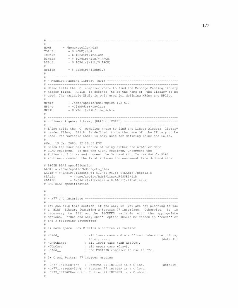
177
# ----------------------------------------------------------------------#HOME = /home/apollo/hda8TOPdir = $(HOME)/hplINCdir = $(TOPdir)/includeBINdir = $(TOPdir)/bin/$(ARCH)LIBdir = $(TOPdir)/lib/$(ARCH)#HPLlib = $(LIBdir)/libhpl.a## ----------------------------------------------------------------------# - Message Passing library (MPI) --------------------------------------# ----------------------------------------------------------------------# MPinc tells the C compiler where to find the Message Passing library# header files, MPlib is defined to be the name of the library to be# used. The variable MPdir is only used for defining MPinc and MPlib.#MPdir = /home/apollo/hda8/mpich-1.2.5.2MPinc = -I$(MPdir)/includeMPlib = $(MPdir)/lib/libmpich.a## ----------------------------------------------------------------------# - Linear Algebra library (BLAS or VSIPL) -----------------------------# ----------------------------------------------------------------------# LAinc tells the C compiler where to find the Linear Algebra library# header files, LAlib is defined to be the name of the library to be# used. The variable LAdir is only used for defining LAinc and LAlib.##Wed, 19 Jan 2005, 22:29:33 EST# Below the user has a choice of using either the ATLAS or Goto# BLAS routines. To use the ATLAS routines, uncomment the# following 2 lines and comment the 3rd and 4th. To use Goto’s BLAS# routines, comment the first 2 lines and uncomment line 3rd and 4th.
# BEGIN BLAS specificationLAdir = /home/apollo/hda8/goto_blasLAlib = $(LAdir)/libgoto_p4_512-r0.96.so $(LAdir)/xerbla.o#LAdir = /home/apollo/hda8/Linux_P4SSE2/lib#LAlib = $(LAdir)/libcblas.a $(LAdir)/libatlas.a# END BLAS specification
## ----------------------------------------------------------------------# - F77 / C interface --------------------------------------------------# ----------------------------------------------------------------------# You can skip this section if and only if you are not planning to use# a BLAS library featuring a Fortran 77 interface. Otherwise, it is# necessary to fill out the F2CDEFS variable with the appropriate# options. **One and only one** option should be chosen in **each** of# the 3 following categories:## 1) name space (How C calls a Fortran 77 routine)## -DAdd_ : all lower case and a suffixed underscore (Suns,# Intel, ...), [default]# -DNoChange : all lower case (IBM RS6000),# -DUpCase : all upper case (Cray),# -DAdd__ : the FORTRAN compiler in use is f2c.## 2) C and Fortran 77 integer mapping## -DF77_INTEGER=int : Fortran 77 INTEGER is a C int, [default]# -DF77_INTEGER=long : Fortran 77 INTEGER is a C long,# -DF77_INTEGER=short : Fortran 77 INTEGER is a C short.#
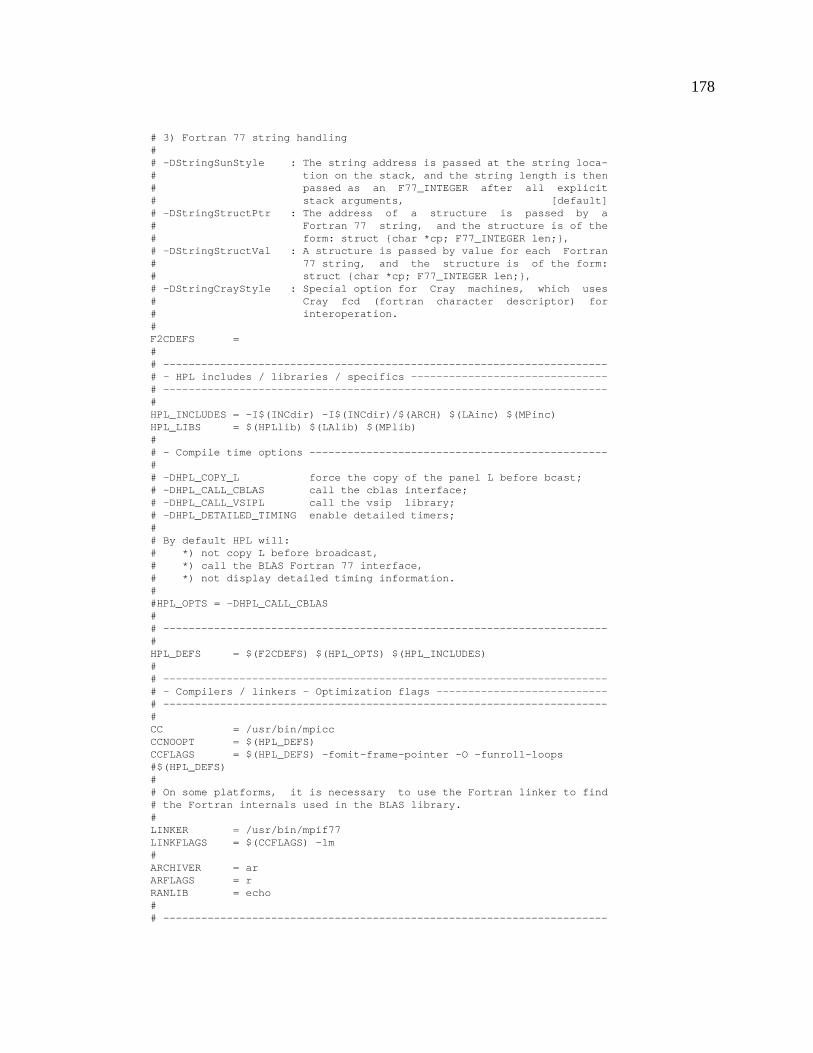
178
# 3) Fortran 77 string handling## -DStringSunStyle : The string address is passed at the string loca-# tion on the stack, and the string length is then# passed as an F77_INTEGER after all explicit# stack arguments, [default]# -DStringStructPtr : The address of a structure is passed by a# Fortran 77 string, and the structure is of the# form: struct {char *cp; F77_INTEGER len;},# -DStringStructVal : A structure is passed by value for each Fortran# 77 string, and the structure is of the form:# struct {char *cp; F77_INTEGER len;},# -DStringCrayStyle : Special option for Cray machines, which uses# Cray fcd (fortran character descriptor) for# interoperation.#F2CDEFS =## ----------------------------------------------------------------------# - HPL includes / libraries / specifics -------------------------------# ----------------------------------------------------------------------#HPL_INCLUDES = -I$(INCdir) -I$(INCdir)/$(ARCH) $(LAinc) $(MPinc)HPL_LIBS = $(HPLlib) $(LAlib) $(MPlib)## - Compile time options -----------------------------------------------## -DHPL_COPY_L force the copy of the panel L before bcast;# -DHPL_CALL_CBLAS call the cblas interface;# -DHPL_CALL_VSIPL call the vsip library;# -DHPL_DETAILED_TIMING enable detailed timers;## By default HPL will:# *) not copy L before broadcast,# *) call the BLAS Fortran 77 interface,# *) not display detailed timing information.##HPL_OPTS = -DHPL_CALL_CBLAS## ----------------------------------------------------------------------#HPL_DEFS = $(F2CDEFS) $(HPL_OPTS) $(HPL_INCLUDES)## ----------------------------------------------------------------------# - Compilers / linkers - Optimization flags ---------------------------# ----------------------------------------------------------------------#CC = /usr/bin/mpiccCCNOOPT = $(HPL_DEFS)CCFLAGS = $(HPL_DEFS) -fomit-frame-pointer -O -funroll-loops#$(HPL_DEFS)## On some platforms, it is necessary to use the Fortran linker to find# the Fortran internals used in the BLAS library.#LINKER = /usr/bin/mpif77LINKFLAGS = $(CCFLAGS) -lm#ARCHIVER = arARFLAGS = rRANLIB = echo## ----------------------------------------------------------------------
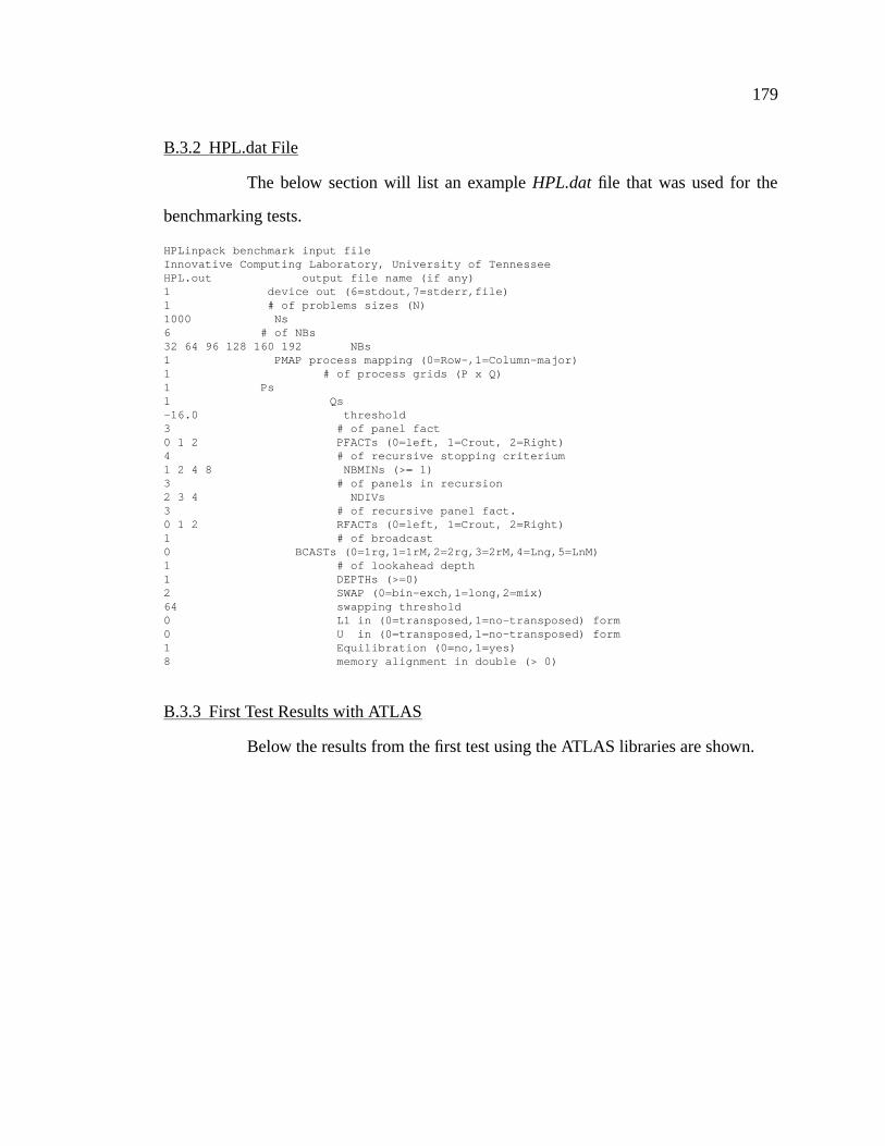
179
B.3.2 HPL.dat File
The below section will list an example HPL.dat file that was used for the
benchmarking tests.
HPLinpack benchmark input fileInnovative Computing Laboratory, University of TennesseeHPL.out output file name (if any)1 device out (6=stdout,7=stderr,file)1 # of problems sizes (N)1000 Ns6 # of NBs32 64 96 128 160 192 NBs1 PMAP process mapping (0=Row-,1=Column-major)1 # of process grids (P x Q)1 Ps1 Qs-16.0 threshold3 # of panel fact0 1 2 PFACTs (0=left, 1=Crout, 2=Right)4 # of recursive stopping criterium1 2 4 8 NBMINs (>= 1)3 # of panels in recursion2 3 4 NDIVs3 # of recursive panel fact.0 1 2 RFACTs (0=left, 1=Crout, 2=Right)1 # of broadcast0 BCASTs (0=1rg,1=1rM,2=2rg,3=2rM,4=Lng,5=LnM)1 # of lookahead depth1 DEPTHs (>=0)2 SWAP (0=bin-exch,1=long,2=mix)64 swapping threshold0 L1 in (0=transposed,1=no-transposed) form0 U in (0=transposed,1=no-transposed) form1 Equilibration (0=no,1=yes)8 memory alignment in double (> 0)
B.3.3 First Test Results with ATLAS
Below the results from the first test using the ATLAS libraries are shown.
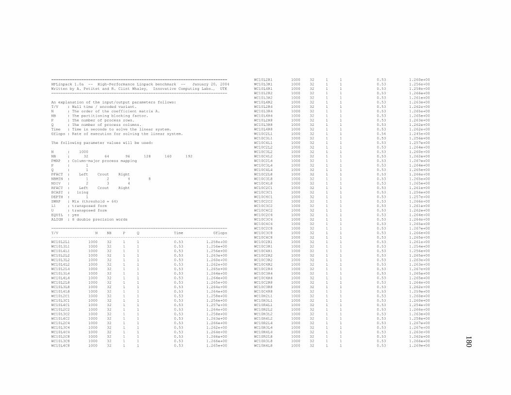
180
============================================================================HPLinpack 1.0a -- High-Performance Linpack benchmark -- January 20, 2004Written by A. Petitet and R. Clint Whaley, Innovative Computing Labs., UTK============================================================================
An explanation of the input/output parameters follows:T/V : Wall time / encoded variant.N : The order of the coefficient matrix A.NB : The partitioning blocking factor.P : The number of process rows.Q : The number of process columns.Time : Time in seconds to solve the linear system.Gflops : Rate of execution for solving the linear system.
The following parameter values will be used:
N : 1000NB : 32 64 96 128 160 192PMAP : Column-major process mappingP : 1Q : 1PFACT : Left Crout RightNBMIN : 1 2 4 8NDIV : 2 3 4RFACT : Left Crout RightBCAST : 1ringDEPTH : 1SWAP : Mix (threshold = 64)L1 : transposed formU : transposed formEQUIL : yesALIGN : 8 double precision words
============================================================================T/V N NB P Q Time Gflops----------------------------------------------------------------------------WC10L2L1 1000 32 1 1 0.53 1.258e+00WC10L3L1 1000 32 1 1 0.53 1.256e+00WC10L4L1 1000 32 1 1 0.53 1.256e+00WC10L2L2 1000 32 1 1 0.53 1.263e+00WC10L3L2 1000 32 1 1 0.53 1.260e+00WC10L4L2 1000 32 1 1 0.53 1.262e+00WC10L2L4 1000 32 1 1 0.53 1.265e+00WC10L3L4 1000 32 1 1 0.53 1.264e+00WC10L4L4 1000 32 1 1 0.53 1.264e+00WC10L2L8 1000 32 1 1 0.53 1.265e+00WC10L3L8 1000 32 1 1 0.53 1.264e+00WC10L4L8 1000 32 1 1 0.53 1.264e+00WC10L2C1 1000 32 1 1 0.53 1.258e+00WC10L3C1 1000 32 1 1 0.53 1.256e+00WC10L4C1 1000 32 1 1 0.53 1.257e+00WC10L2C2 1000 32 1 1 0.53 1.264e+00WC10L3C2 1000 32 1 1 0.53 1.258e+00WC10L4C2 1000 32 1 1 0.53 1.263e+00WC10L2C4 1000 32 1 1 0.53 1.266e+00WC10L3C4 1000 32 1 1 0.53 1.262e+00WC10L4C4 1000 32 1 1 0.53 1.264e+00WC10L2C8 1000 32 1 1 0.53 1.266e+00WC10L3C8 1000 32 1 1 0.53 1.266e+00WC10L4C8 1000 32 1 1 0.53 1.265e+00
WC10L2R1 1000 32 1 1 0.53 1.260e+00WC10L3R1 1000 32 1 1 0.53 1.256e+00WC10L4R1 1000 32 1 1 0.53 1.258e+00WC10L2R2 1000 32 1 1 0.53 1.266e+00WC10L3R2 1000 32 1 1 0.53 1.261e+00WC10L4R2 1000 32 1 1 0.53 1.263e+00WC10L2R4 1000 32 1 1 0.53 1.262e+00WC10L3R4 1000 32 1 1 0.53 1.265e+00WC10L4R4 1000 32 1 1 0.53 1.265e+00WC10L2R8 1000 32 1 1 0.53 1.263e+00WC10L3R8 1000 32 1 1 0.53 1.262e+00WC10L4R8 1000 32 1 1 0.53 1.262e+00WC10C2L1 1000 32 1 1 0.54 1.245e+00WC10C3L1 1000 32 1 1 0.53 1.256e+00WC10C4L1 1000 32 1 1 0.53 1.257e+00WC10C2L2 1000 32 1 1 0.53 1.264e+00WC10C3L2 1000 32 1 1 0.53 1.260e+00WC10C4L2 1000 32 1 1 0.53 1.262e+00WC10C2L4 1000 32 1 1 0.53 1.267e+00WC10C3L4 1000 32 1 1 0.53 1.264e+00WC10C4L4 1000 32 1 1 0.53 1.265e+00WC10C2L8 1000 32 1 1 0.53 1.266e+00WC10C3L8 1000 32 1 1 0.53 1.265e+00WC10C4L8 1000 32 1 1 0.53 1.265e+00WC10C2C1 1000 32 1 1 0.53 1.261e+00WC10C3C1 1000 32 1 1 0.53 1.256e+00WC10C4C1 1000 32 1 1 0.53 1.257e+00WC10C2C2 1000 32 1 1 0.53 1.266e+00WC10C3C2 1000 32 1 1 0.53 1.261e+00WC10C4C2 1000 32 1 1 0.53 1.262e+00WC10C2C4 1000 32 1 1 0.53 1.264e+00WC10C3C4 1000 32 1 1 0.53 1.264e+00WC10C4C4 1000 32 1 1 0.53 1.265e+00WC10C2C8 1000 32 1 1 0.53 1.267e+00WC10C3C8 1000 32 1 1 0.53 1.266e+00WC10C4C8 1000 32 1 1 0.53 1.265e+00WC10C2R1 1000 32 1 1 0.53 1.261e+00WC10C3R1 1000 32 1 1 0.53 1.254e+00WC10C4R1 1000 32 1 1 0.53 1.256e+00WC10C2R2 1000 32 1 1 0.53 1.265e+00WC10C3R2 1000 32 1 1 0.53 1.263e+00WC10C4R2 1000 32 1 1 0.53 1.263e+00WC10C2R4 1000 32 1 1 0.53 1.267e+00WC10C3R4 1000 32 1 1 0.53 1.265e+00WC10C4R4 1000 32 1 1 0.53 1.265e+00WC10C2R8 1000 32 1 1 0.53 1.264e+00WC10C3R8 1000 32 1 1 0.53 1.262e+00WC10C4R8 1000 32 1 1 0.53 1.259e+00WC10R2L1 1000 32 1 1 0.53 1.260e+00WC10R3L1 1000 32 1 1 0.53 1.260e+00WC10R4L1 1000 32 1 1 0.53 1.254e+00WC10R2L2 1000 32 1 1 0.53 1.266e+00WC10R3L2 1000 32 1 1 0.53 1.263e+00WC10R4L2 1000 32 1 1 0.53 1.258e+00WC10R2L4 1000 32 1 1 0.53 1.267e+00WC10R3L4 1000 32 1 1 0.53 1.267e+00WC10R4L4 1000 32 1 1 0.53 1.263e+00WC10R2L8 1000 32 1 1 0.53 1.262e+00WC10R3L8 1000 32 1 1 0.53 1.266e+00WC10R4L8 1000 32 1 1 0.53 1.269e+00
181
WC10R2C1 1000 32 1 1 0.53 1.261e+00WC10R3C1 1000 32 1 1 0.53 1.259e+00WC10R4C1 1000 32 1 1 0.53 1.254e+00WC10R2C2 1000 32 1 1 0.53 1.265e+00WC10R3C2 1000 32 1 1 0.53 1.250e+00WC10R4C2 1000 32 1 1 0.53 1.260e+00WC10R2C4 1000 32 1 1 0.53 1.267e+00WC10R3C4 1000 32 1 1 0.53 1.267e+00WC10R4C4 1000 32 1 1 0.53 1.268e+00WC10R2C8 1000 32 1 1 0.53 1.268e+00WC10R3C8 1000 32 1 1 0.53 1.267e+00WC10R4C8 1000 32 1 1 0.53 1.269e+00WC10R2R1 1000 32 1 1 0.53 1.260e+00WC10R3R1 1000 32 1 1 0.53 1.257e+00WC10R4R1 1000 32 1 1 0.53 1.254e+00WC10R2R2 1000 32 1 1 0.53 1.267e+00WC10R3R2 1000 32 1 1 0.53 1.264e+00WC10R4R2 1000 32 1 1 0.53 1.260e+00WC10R2R4 1000 32 1 1 0.53 1.267e+00WC10R3R4 1000 32 1 1 0.53 1.267e+00WC10R4R4 1000 32 1 1 0.53 1.268e+00WC10R2R8 1000 32 1 1 0.53 1.263e+00WC10R3R8 1000 32 1 1 0.53 1.257e+00WC10R4R8 1000 32 1 1 0.53 1.266e+00WC10L2L1 1000 64 1 1 0.49 1.371e+00WC10L3L1 1000 64 1 1 0.49 1.368e+00WC10L4L1 1000 64 1 1 0.49 1.362e+00WC10L2L2 1000 64 1 1 0.49 1.375e+00WC10L3L2 1000 64 1 1 0.49 1.371e+00WC10L4L2 1000 64 1 1 0.49 1.365e+00WC10L2L4 1000 64 1 1 0.48 1.378e+00WC10L3L4 1000 64 1 1 0.49 1.373e+00WC10L4L4 1000 64 1 1 0.49 1.369e+00WC10L2L8 1000 64 1 1 0.48 1.380e+00WC10L3L8 1000 64 1 1 0.49 1.377e+00WC10L4L8 1000 64 1 1 0.49 1.372e+00WC10L2C1 1000 64 1 1 0.49 1.373e+00WC10L3C1 1000 64 1 1 0.49 1.369e+00WC10L4C1 1000 64 1 1 0.49 1.363e+00WC10L2C2 1000 64 1 1 0.49 1.377e+00WC10L3C2 1000 64 1 1 0.49 1.370e+00WC10L4C2 1000 64 1 1 0.49 1.366e+00WC10L2C4 1000 64 1 1 0.48 1.380e+00WC10L3C4 1000 64 1 1 0.49 1.375e+00WC10L4C4 1000 64 1 1 0.49 1.369e+00WC10L2C8 1000 64 1 1 0.48 1.380e+00WC10L3C8 1000 64 1 1 0.49 1.376e+00WC10L4C8 1000 64 1 1 0.49 1.373e+00WC10L2R1 1000 64 1 1 0.49 1.372e+00WC10L3R1 1000 64 1 1 0.49 1.366e+00WC10L4R1 1000 64 1 1 0.49 1.357e+00WC10L2R2 1000 64 1 1 0.48 1.378e+00WC10L3R2 1000 64 1 1 0.49 1.374e+00WC10L4R2 1000 64 1 1 0.49 1.367e+00WC10L2R4 1000 64 1 1 0.48 1.381e+00WC10L3R4 1000 64 1 1 0.49 1.377e+00WC10L4R4 1000 64 1 1 0.49 1.371e+00WC10L2R8 1000 64 1 1 0.48 1.378e+00WC10L3R8 1000 64 1 1 0.49 1.372e+00WC10L4R8 1000 64 1 1 0.49 1.353e+00
WC10C2L1 1000 64 1 1 0.49 1.372e+00WC10C3L1 1000 64 1 1 0.49 1.368e+00WC10C4L1 1000 64 1 1 0.49 1.365e+00WC10C2L2 1000 64 1 1 0.49 1.376e+00WC10C3L2 1000 64 1 1 0.49 1.371e+00WC10C4L2 1000 64 1 1 0.49 1.366e+00WC10C2L4 1000 64 1 1 0.48 1.379e+00WC10C3L4 1000 64 1 1 0.49 1.375e+00WC10C4L4 1000 64 1 1 0.49 1.367e+00WC10C2L8 1000 64 1 1 0.48 1.381e+00WC10C3L8 1000 64 1 1 0.49 1.375e+00WC10C4L8 1000 64 1 1 0.49 1.373e+00WC10C2C1 1000 64 1 1 0.49 1.372e+00WC10C3C1 1000 64 1 1 0.49 1.368e+00WC10C4C1 1000 64 1 1 0.49 1.362e+00WC10C2C2 1000 64 1 1 0.49 1.376e+00WC10C3C2 1000 64 1 1 0.49 1.375e+00WC10C4C2 1000 64 1 1 0.49 1.364e+00WC10C2C4 1000 64 1 1 0.48 1.380e+00WC10C3C4 1000 64 1 1 0.49 1.375e+00WC10C4C4 1000 64 1 1 0.49 1.368e+00WC10C2C8 1000 64 1 1 0.48 1.381e+00WC10C3C8 1000 64 1 1 0.49 1.374e+00WC10C4C8 1000 64 1 1 0.49 1.372e+00WC10C2R1 1000 64 1 1 0.49 1.371e+00WC10C3R1 1000 64 1 1 0.49 1.366e+00WC10C4R1 1000 64 1 1 0.49 1.361e+00WC10C2R2 1000 64 1 1 0.49 1.376e+00WC10C3R2 1000 64 1 1 0.49 1.374e+00WC10C4R2 1000 64 1 1 0.49 1.368e+00WC10C2R4 1000 64 1 1 0.48 1.383e+00WC10C3R4 1000 64 1 1 0.49 1.376e+00WC10C4R4 1000 64 1 1 0.49 1.371e+00WC10C2R8 1000 64 1 1 0.48 1.378e+00WC10C3R8 1000 64 1 1 0.49 1.371e+00WC10C4R8 1000 64 1 1 0.49 1.371e+00WC10R2L1 1000 64 1 1 0.49 1.370e+00WC10R3L1 1000 64 1 1 0.49 1.372e+00WC10R4L1 1000 64 1 1 0.49 1.370e+00WC10R2L2 1000 64 1 1 0.49 1.377e+00WC10R3L2 1000 64 1 1 0.48 1.378e+00WC10R4L2 1000 64 1 1 0.49 1.377e+00WC10R2L4 1000 64 1 1 0.48 1.380e+00WC10R3L4 1000 64 1 1 0.48 1.379e+00WC10R4L4 1000 64 1 1 0.48 1.383e+00WC10R2L8 1000 64 1 1 0.49 1.372e+00WC10R3L8 1000 64 1 1 0.48 1.380e+00WC10R4L8 1000 64 1 1 0.48 1.383e+00WC10R2C1 1000 64 1 1 0.49 1.373e+00WC10R3C1 1000 64 1 1 0.49 1.372e+00WC10R4C1 1000 64 1 1 0.49 1.371e+00WC10R2C2 1000 64 1 1 0.49 1.377e+00WC10R3C2 1000 64 1 1 0.48 1.379e+00WC10R4C2 1000 64 1 1 0.49 1.377e+00WC10R2C4 1000 64 1 1 0.48 1.380e+00WC10R3C4 1000 64 1 1 0.49 1.367e+00WC10R4C4 1000 64 1 1 0.48 1.381e+00WC10R2C8 1000 64 1 1 0.48 1.380e+00WC10R3C8 1000 64 1 1 0.48 1.379e+00WC10R4C8 1000 64 1 1 0.48 1.383e+00
182
WC10R2R1 1000 64 1 1 0.49 1.372e+00WC10R3R1 1000 64 1 1 0.49 1.371e+00WC10R4R1 1000 64 1 1 0.49 1.370e+00WC10R2R2 1000 64 1 1 0.49 1.378e+00WC10R3R2 1000 64 1 1 0.49 1.377e+00WC10R4R2 1000 64 1 1 0.48 1.378e+00WC10R2R4 1000 64 1 1 0.48 1.380e+00WC10R3R4 1000 64 1 1 0.48 1.380e+00WC10R4R4 1000 64 1 1 0.48 1.382e+00WC10R2R8 1000 64 1 1 0.49 1.376e+00WC10R3R8 1000 64 1 1 0.49 1.377e+00WC10R4R8 1000 64 1 1 0.48 1.378e+00WC10L2L1 1000 96 1 1 0.38 1.764e+00WC10L3L1 1000 96 1 1 0.38 1.748e+00WC10L4L1 1000 96 1 1 0.38 1.768e+00WC10L2L2 1000 96 1 1 0.38 1.773e+00WC10L3L2 1000 96 1 1 0.38 1.759e+00WC10L4L2 1000 96 1 1 0.37 1.784e+00WC10L2L4 1000 96 1 1 0.37 1.783e+00WC10L3L4 1000 96 1 1 0.38 1.766e+00WC10L4L4 1000 96 1 1 0.37 1.786e+00WC10L2L8 1000 96 1 1 0.38 1.779e+00WC10L3L8 1000 96 1 1 0.38 1.768e+00WC10L4L8 1000 96 1 1 0.37 1.787e+00WC10L2C1 1000 96 1 1 0.38 1.770e+00WC10L3C1 1000 96 1 1 0.38 1.751e+00WC10L4C1 1000 96 1 1 0.38 1.770e+00WC10L2C2 1000 96 1 1 0.38 1.775e+00WC10L3C2 1000 96 1 1 0.38 1.762e+00WC10L4C2 1000 96 1 1 0.38 1.781e+00WC10L2C4 1000 96 1 1 0.38 1.777e+00WC10L3C4 1000 96 1 1 0.38 1.773e+00WC10L4C4 1000 96 1 1 0.37 1.792e+00WC10L2C8 1000 96 1 1 0.38 1.778e+00WC10L3C8 1000 96 1 1 0.38 1.770e+00WC10L4C8 1000 96 1 1 0.37 1.787e+00WC10L2R1 1000 96 1 1 0.38 1.765e+00WC10L3R1 1000 96 1 1 0.38 1.745e+00WC10L4R1 1000 96 1 1 0.38 1.777e+00WC10L2R2 1000 96 1 1 0.37 1.782e+00WC10L3R2 1000 96 1 1 0.38 1.766e+00WC10L4R2 1000 96 1 1 0.37 1.783e+00WC10L2R4 1000 96 1 1 0.38 1.781e+00WC10L3R4 1000 96 1 1 0.38 1.769e+00WC10L4R4 1000 96 1 1 0.37 1.789e+00WC10L2R8 1000 96 1 1 0.38 1.780e+00WC10L3R8 1000 96 1 1 0.38 1.773e+00WC10L4R8 1000 96 1 1 0.38 1.774e+00WC10C2L1 1000 96 1 1 0.38 1.765e+00WC10C3L1 1000 96 1 1 0.38 1.746e+00WC10C4L1 1000 96 1 1 0.38 1.773e+00WC10C2L2 1000 96 1 1 0.38 1.773e+00WC10C3L2 1000 96 1 1 0.38 1.763e+00WC10C4L2 1000 96 1 1 0.37 1.785e+00WC10C2L4 1000 96 1 1 0.38 1.779e+00WC10C3L4 1000 96 1 1 0.38 1.767e+00WC10C4L4 1000 96 1 1 0.37 1.785e+00WC10C2L8 1000 96 1 1 0.38 1.780e+00WC10C3L8 1000 96 1 1 0.38 1.772e+00WC10C4L8 1000 96 1 1 0.37 1.792e+00
WC10C2C1 1000 96 1 1 0.38 1.766e+00WC10C3C1 1000 96 1 1 0.39 1.715e+00WC10C4C1 1000 96 1 1 0.38 1.773e+00WC10C2C2 1000 96 1 1 0.38 1.776e+00WC10C3C2 1000 96 1 1 0.38 1.760e+00WC10C4C2 1000 96 1 1 0.37 1.787e+00WC10C2C4 1000 96 1 1 0.37 1.782e+00WC10C3C4 1000 96 1 1 0.38 1.766e+00WC10C4C4 1000 96 1 1 0.37 1.782e+00WC10C2C8 1000 96 1 1 0.38 1.779e+00WC10C3C8 1000 96 1 1 0.38 1.770e+00WC10C4C8 1000 96 1 1 0.37 1.785e+00WC10C2R1 1000 96 1 1 0.38 1.769e+00WC10C3R1 1000 96 1 1 0.38 1.751e+00WC10C4R1 1000 96 1 1 0.38 1.771e+00WC10C2R2 1000 96 1 1 0.38 1.777e+00WC10C3R2 1000 96 1 1 0.38 1.762e+00WC10C4R2 1000 96 1 1 0.37 1.784e+00WC10C2R4 1000 96 1 1 0.38 1.779e+00WC10C3R4 1000 96 1 1 0.38 1.773e+00WC10C4R4 1000 96 1 1 0.37 1.791e+00WC10C2R8 1000 96 1 1 0.38 1.776e+00WC10C3R8 1000 96 1 1 0.38 1.768e+00WC10C4R8 1000 96 1 1 0.37 1.784e+00WC10R2L1 1000 96 1 1 0.38 1.760e+00WC10R3L1 1000 96 1 1 0.38 1.758e+00WC10R4L1 1000 96 1 1 0.38 1.769e+00WC10R2L2 1000 96 1 1 0.38 1.779e+00WC10R3L2 1000 96 1 1 0.38 1.767e+00WC10R4L2 1000 96 1 1 0.38 1.770e+00WC10R2L4 1000 96 1 1 0.38 1.775e+00WC10R3L4 1000 96 1 1 0.38 1.774e+00WC10R4L4 1000 96 1 1 0.38 1.779e+00WC10R2L8 1000 96 1 1 0.37 1.785e+00WC10R3L8 1000 96 1 1 0.38 1.781e+00WC10R4L8 1000 96 1 1 0.37 1.782e+00WC10R2C1 1000 96 1 1 0.38 1.762e+00WC10R3C1 1000 96 1 1 0.38 1.760e+00WC10R4C1 1000 96 1 1 0.38 1.762e+00WC10R2C2 1000 96 1 1 0.38 1.775e+00WC10R3C2 1000 96 1 1 0.38 1.775e+00WC10R4C2 1000 96 1 1 0.38 1.774e+00WC10R2C4 1000 96 1 1 0.38 1.777e+00WC10R3C4 1000 96 1 1 0.38 1.775e+00WC10R4C4 1000 96 1 1 0.38 1.780e+00WC10R2C8 1000 96 1 1 0.38 1.778e+00WC10R3C8 1000 96 1 1 0.38 1.776e+00WC10R4C8 1000 96 1 1 0.37 1.784e+00WC10R2R1 1000 96 1 1 0.38 1.771e+00WC10R3R1 1000 96 1 1 0.38 1.760e+00WC10R4R1 1000 96 1 1 0.38 1.764e+00WC10R2R2 1000 96 1 1 0.38 1.779e+00WC10R3R2 1000 96 1 1 0.38 1.774e+00WC10R4R2 1000 96 1 1 0.38 1.773e+00WC10R2R4 1000 96 1 1 0.38 1.782e+00WC10R3R4 1000 96 1 1 0.37 1.784e+00WC10R4R4 1000 96 1 1 0.38 1.770e+00WC10R2R8 1000 96 1 1 0.38 1.775e+00WC10R3R8 1000 96 1 1 0.38 1.773e+00WC10R4R8 1000 96 1 1 0.38 1.773e+00
183
WC10L2L1 1000 128 1 1 0.40 1.686e+00WC10L3L1 1000 128 1 1 0.39 1.703e+00WC10L4L1 1000 128 1 1 0.39 1.697e+00WC10L2L2 1000 128 1 1 0.39 1.693e+00WC10L3L2 1000 128 1 1 0.39 1.705e+00WC10L4L2 1000 128 1 1 0.39 1.695e+00WC10L2L4 1000 128 1 1 0.39 1.698e+00WC10L3L4 1000 128 1 1 0.39 1.713e+00WC10L4L4 1000 128 1 1 0.39 1.705e+00WC10L2L8 1000 128 1 1 0.39 1.698e+00WC10L3L8 1000 128 1 1 0.39 1.714e+00WC10L4L8 1000 128 1 1 0.39 1.701e+00WC10L2C1 1000 128 1 1 0.40 1.686e+00WC10L3C1 1000 128 1 1 0.39 1.699e+00WC10L4C1 1000 128 1 1 0.39 1.692e+00WC10L2C2 1000 128 1 1 0.40 1.691e+00WC10L3C2 1000 128 1 1 0.39 1.702e+00WC10L4C2 1000 128 1 1 0.39 1.698e+00WC10L2C4 1000 128 1 1 0.39 1.702e+00WC10L3C4 1000 128 1 1 0.39 1.715e+00WC10L4C4 1000 128 1 1 0.39 1.702e+00WC10L2C8 1000 128 1 1 0.39 1.696e+00WC10L3C8 1000 128 1 1 0.39 1.705e+00WC10L4C8 1000 128 1 1 0.39 1.701e+00WC10L2R1 1000 128 1 1 0.40 1.685e+00WC10L3R1 1000 128 1 1 0.39 1.697e+00WC10L4R1 1000 128 1 1 0.39 1.692e+00WC10L2R2 1000 128 1 1 0.39 1.697e+00WC10L3R2 1000 128 1 1 0.39 1.712e+00WC10L4R2 1000 128 1 1 0.39 1.701e+00WC10L2R4 1000 128 1 1 0.39 1.699e+00WC10L3R4 1000 128 1 1 0.39 1.713e+00WC10L4R4 1000 128 1 1 0.39 1.706e+00WC10L2R8 1000 128 1 1 0.39 1.693e+00WC10L3R8 1000 128 1 1 0.39 1.706e+00WC10L4R8 1000 128 1 1 0.39 1.703e+00WC10C2L1 1000 128 1 1 0.40 1.687e+00WC10C3L1 1000 128 1 1 0.39 1.702e+00WC10C4L1 1000 128 1 1 0.40 1.687e+00WC10C2L2 1000 128 1 1 0.40 1.690e+00WC10C3L2 1000 128 1 1 0.39 1.703e+00WC10C4L2 1000 128 1 1 0.39 1.694e+00WC10C2L4 1000 128 1 1 0.39 1.697e+00WC10C3L4 1000 128 1 1 0.39 1.712e+00WC10C4L4 1000 128 1 1 0.39 1.700e+00WC10C2L8 1000 128 1 1 0.39 1.703e+00WC10C3L8 1000 128 1 1 0.39 1.714e+00WC10C4L8 1000 128 1 1 0.39 1.704e+00WC10C2C1 1000 128 1 1 0.40 1.685e+00WC10C3C1 1000 128 1 1 0.39 1.699e+00WC10C4C1 1000 128 1 1 0.40 1.690e+00WC10C2C2 1000 128 1 1 0.39 1.693e+00WC10C3C2 1000 128 1 1 0.39 1.706e+00WC10C4C2 1000 128 1 1 0.39 1.698e+00WC10C2C4 1000 128 1 1 0.39 1.701e+00WC10C3C4 1000 128 1 1 0.39 1.717e+00WC10C4C4 1000 128 1 1 0.39 1.699e+00WC10C2C8 1000 128 1 1 0.39 1.699e+00WC10C3C8 1000 128 1 1 0.39 1.709e+00WC10C4C8 1000 128 1 1 0.39 1.703e+00
WC10C2R1 1000 128 1 1 0.40 1.684e+00WC10C3R1 1000 128 1 1 0.39 1.699e+00WC10C4R1 1000 128 1 1 0.40 1.679e+00WC10C2R2 1000 128 1 1 0.39 1.697e+00WC10C3R2 1000 128 1 1 0.39 1.713e+00WC10C4R2 1000 128 1 1 0.39 1.700e+00WC10C2R4 1000 128 1 1 0.39 1.700e+00WC10C3R4 1000 128 1 1 0.39 1.711e+00WC10C4R4 1000 128 1 1 0.39 1.705e+00WC10C2R8 1000 128 1 1 0.39 1.698e+00WC10C3R8 1000 128 1 1 0.39 1.707e+00WC10C4R8 1000 128 1 1 0.39 1.701e+00WC10R2L1 1000 128 1 1 0.40 1.688e+00WC10R3L1 1000 128 1 1 0.39 1.693e+00WC10R4L1 1000 128 1 1 0.40 1.681e+00WC10R2L2 1000 128 1 1 0.40 1.690e+00WC10R3L2 1000 128 1 1 0.39 1.694e+00WC10R4L2 1000 128 1 1 0.40 1.687e+00WC10R2L4 1000 128 1 1 0.40 1.663e+00WC10R3L4 1000 128 1 1 0.39 1.704e+00WC10R4L4 1000 128 1 1 0.39 1.708e+00WC10R2L8 1000 128 1 1 0.39 1.703e+00WC10R3L8 1000 128 1 1 0.39 1.701e+00WC10R4L8 1000 128 1 1 0.39 1.705e+00WC10R2C1 1000 128 1 1 0.40 1.686e+00WC10R3C1 1000 128 1 1 0.40 1.686e+00WC10R4C1 1000 128 1 1 0.40 1.681e+00WC10R2C2 1000 128 1 1 0.40 1.691e+00WC10R3C2 1000 128 1 1 0.39 1.693e+00WC10R4C2 1000 128 1 1 0.39 1.692e+00WC10R2C4 1000 128 1 1 0.39 1.701e+00WC10R3C4 1000 128 1 1 0.39 1.702e+00WC10R4C4 1000 128 1 1 0.39 1.703e+00WC10R2C8 1000 128 1 1 0.39 1.696e+00WC10R3C8 1000 128 1 1 0.39 1.701e+00WC10R4C8 1000 128 1 1 0.39 1.704e+00WC10R2R1 1000 128 1 1 0.40 1.683e+00WC10R3R1 1000 128 1 1 0.40 1.688e+00WC10R4R1 1000 128 1 1 0.40 1.686e+00WC10R2R2 1000 128 1 1 0.39 1.699e+00WC10R3R2 1000 128 1 1 0.39 1.698e+00WC10R4R2 1000 128 1 1 0.40 1.686e+00WC10R2R4 1000 128 1 1 0.39 1.699e+00WC10R3R4 1000 128 1 1 0.39 1.705e+00WC10R4R4 1000 128 1 1 0.39 1.705e+00WC10R2R8 1000 128 1 1 0.39 1.694e+00WC10R3R8 1000 128 1 1 0.39 1.701e+00WC10R4R8 1000 128 1 1 0.39 1.704e+00WC10L2L1 1000 160 1 1 0.35 1.884e+00WC10L3L1 1000 160 1 1 0.36 1.859e+00WC10L4L1 1000 160 1 1 0.36 1.856e+00WC10L2L2 1000 160 1 1 0.35 1.884e+00WC10L3L2 1000 160 1 1 0.36 1.862e+00WC10L4L2 1000 160 1 1 0.36 1.867e+00WC10L2L4 1000 160 1 1 0.35 1.899e+00WC10L3L4 1000 160 1 1 0.36 1.864e+00WC10L4L4 1000 160 1 1 0.36 1.865e+00WC10L2L8 1000 160 1 1 0.35 1.894e+00WC10L3L8 1000 160 1 1 0.36 1.876e+00WC10L4L8 1000 160 1 1 0.35 1.884e+00
184
WC10L2C1 1000 160 1 1 0.36 1.880e+00WC10L3C1 1000 160 1 1 0.36 1.860e+00WC10L4C1 1000 160 1 1 0.36 1.856e+00WC10L2C2 1000 160 1 1 0.35 1.886e+00WC10L3C2 1000 160 1 1 0.36 1.874e+00WC10L4C2 1000 160 1 1 0.36 1.860e+00WC10L2C4 1000 160 1 1 0.35 1.894e+00WC10L3C4 1000 160 1 1 0.36 1.865e+00WC10L4C4 1000 160 1 1 0.36 1.863e+00WC10L2C8 1000 160 1 1 0.35 1.897e+00WC10L3C8 1000 160 1 1 0.36 1.861e+00WC10L4C8 1000 160 1 1 0.36 1.877e+00WC10L2R1 1000 160 1 1 0.36 1.877e+00WC10L3R1 1000 160 1 1 0.36 1.859e+00WC10L4R1 1000 160 1 1 0.36 1.856e+00WC10L2R2 1000 160 1 1 0.35 1.894e+00WC10L3R2 1000 160 1 1 0.36 1.872e+00WC10L4R2 1000 160 1 1 0.36 1.866e+00WC10L2R4 1000 160 1 1 0.35 1.899e+00WC10L3R4 1000 160 1 1 0.36 1.871e+00WC10L4R4 1000 160 1 1 0.36 1.876e+00WC10L2R8 1000 160 1 1 0.35 1.899e+00WC10L3R8 1000 160 1 1 0.36 1.869e+00WC10L4R8 1000 160 1 1 0.36 1.877e+00WC10C2L1 1000 160 1 1 0.36 1.879e+00WC10C3L1 1000 160 1 1 0.36 1.865e+00WC10C4L1 1000 160 1 1 0.36 1.859e+00WC10C2L2 1000 160 1 1 0.35 1.886e+00WC10C3L2 1000 160 1 1 0.36 1.867e+00WC10C4L2 1000 160 1 1 0.37 1.827e+00WC10C2L4 1000 160 1 1 0.35 1.894e+00WC10C3L4 1000 160 1 1 0.36 1.871e+00WC10C4L4 1000 160 1 1 0.36 1.866e+00WC10C2L8 1000 160 1 1 0.35 1.896e+00WC10C3L8 1000 160 1 1 0.36 1.871e+00WC10C4L8 1000 160 1 1 0.36 1.878e+00WC10C2C1 1000 160 1 1 0.35 1.884e+00WC10C3C1 1000 160 1 1 0.36 1.863e+00WC10C4C1 1000 160 1 1 0.36 1.854e+00WC10C2C2 1000 160 1 1 0.35 1.888e+00WC10C3C2 1000 160 1 1 0.36 1.867e+00WC10C4C2 1000 160 1 1 0.36 1.869e+00WC10C2C4 1000 160 1 1 0.35 1.898e+00WC10C3C4 1000 160 1 1 0.36 1.864e+00WC10C4C4 1000 160 1 1 0.36 1.865e+00WC10C2C8 1000 160 1 1 0.35 1.894e+00WC10C3C8 1000 160 1 1 0.36 1.867e+00WC10C4C8 1000 160 1 1 0.35 1.883e+00WC10C2R1 1000 160 1 1 0.36 1.878e+00WC10C3R1 1000 160 1 1 0.36 1.858e+00WC10C4R1 1000 160 1 1 0.36 1.851e+00WC10C2R2 1000 160 1 1 0.35 1.891e+00WC10C3R2 1000 160 1 1 0.36 1.876e+00WC10C4R2 1000 160 1 1 0.36 1.874e+00WC10C2R4 1000 160 1 1 0.35 1.892e+00WC10C3R4 1000 160 1 1 0.36 1.868e+00WC10C4R4 1000 160 1 1 0.36 1.869e+00WC10C2R8 1000 160 1 1 0.35 1.893e+00WC10C3R8 1000 160 1 1 0.36 1.873e+00WC10C4R8 1000 160 1 1 0.36 1.877e+00
WC10R2L1 1000 160 1 1 0.36 1.876e+00WC10R3L1 1000 160 1 1 0.36 1.837e+00WC10R4L1 1000 160 1 1 0.36 1.834e+00WC10R2L2 1000 160 1 1 0.35 1.891e+00WC10R3L2 1000 160 1 1 0.36 1.849e+00WC10R4L2 1000 160 1 1 0.36 1.855e+00WC10R2L4 1000 160 1 1 0.35 1.889e+00WC10R3L4 1000 160 1 1 0.36 1.861e+00WC10R4L4 1000 160 1 1 0.36 1.858e+00WC10R2L8 1000 160 1 1 0.35 1.901e+00WC10R3L8 1000 160 1 1 0.36 1.864e+00WC10R4L8 1000 160 1 1 0.36 1.866e+00WC10R2C1 1000 160 1 1 0.36 1.877e+00WC10R3C1 1000 160 1 1 0.36 1.835e+00WC10R4C1 1000 160 1 1 0.36 1.837e+00WC10R2C2 1000 160 1 1 0.35 1.891e+00WC10R3C2 1000 160 1 1 0.36 1.846e+00WC10R4C2 1000 160 1 1 0.36 1.855e+00WC10R2C4 1000 160 1 1 0.35 1.890e+00WC10R3C4 1000 160 1 1 0.36 1.861e+00WC10R4C4 1000 160 1 1 0.36 1.861e+00WC10R2C8 1000 160 1 1 0.35 1.893e+00WC10R3C8 1000 160 1 1 0.36 1.849e+00WC10R4C8 1000 160 1 1 0.36 1.864e+00WC10R2R1 1000 160 1 1 0.36 1.876e+00WC10R3R1 1000 160 1 1 0.36 1.842e+00WC10R4R1 1000 160 1 1 0.36 1.839e+00WC10R2R2 1000 160 1 1 0.35 1.889e+00WC10R3R2 1000 160 1 1 0.36 1.850e+00WC10R4R2 1000 160 1 1 0.36 1.859e+00WC10R2R4 1000 160 1 1 0.35 1.892e+00WC10R3R4 1000 160 1 1 0.36 1.868e+00WC10R4R4 1000 160 1 1 0.36 1.861e+00WC10R2R8 1000 160 1 1 0.35 1.892e+00WC10R3R8 1000 160 1 1 0.36 1.861e+00WC10R4R8 1000 160 1 1 0.36 1.863e+00WC10L2L1 1000 192 1 1 0.37 1.792e+00WC10L3L1 1000 192 1 1 0.38 1.753e+00WC10L4L1 1000 192 1 1 0.37 1.788e+00WC10L2L2 1000 192 1 1 0.37 1.795e+00WC10L3L2 1000 192 1 1 0.38 1.753e+00WC10L4L2 1000 192 1 1 0.37 1.793e+00WC10L2L4 1000 192 1 1 0.38 1.757e+00WC10L3L4 1000 192 1 1 0.38 1.767e+00WC10L4L4 1000 192 1 1 0.37 1.805e+00WC10L2L8 1000 192 1 1 0.37 1.804e+00WC10L3L8 1000 192 1 1 0.38 1.768e+00WC10L4L8 1000 192 1 1 0.37 1.803e+00WC10L2C1 1000 192 1 1 0.37 1.788e+00WC10L3C1 1000 192 1 1 0.38 1.753e+00WC10L4C1 1000 192 1 1 0.37 1.793e+00WC10L2C2 1000 192 1 1 0.37 1.796e+00WC10L3C2 1000 192 1 1 0.38 1.755e+00WC10L4C2 1000 192 1 1 0.37 1.796e+00WC10L2C4 1000 192 1 1 0.37 1.798e+00WC10L3C4 1000 192 1 1 0.38 1.763e+00WC10L4C4 1000 192 1 1 0.37 1.807e+00WC10L2C8 1000 192 1 1 0.37 1.807e+00WC10L3C8 1000 192 1 1 0.38 1.766e+00WC10L4C8 1000 192 1 1 0.37 1.803e+00
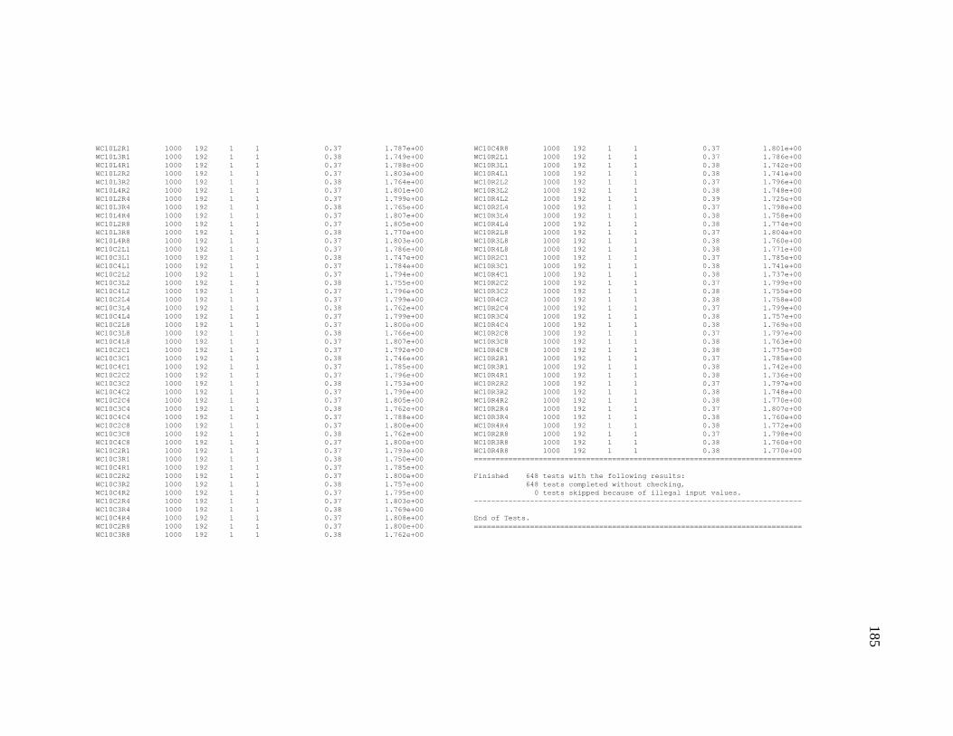
185
WC10L2R1 1000 192 1 1 0.37 1.787e+00WC10L3R1 1000 192 1 1 0.38 1.749e+00WC10L4R1 1000 192 1 1 0.37 1.788e+00WC10L2R2 1000 192 1 1 0.37 1.803e+00WC10L3R2 1000 192 1 1 0.38 1.764e+00WC10L4R2 1000 192 1 1 0.37 1.801e+00WC10L2R4 1000 192 1 1 0.37 1.799e+00WC10L3R4 1000 192 1 1 0.38 1.765e+00WC10L4R4 1000 192 1 1 0.37 1.807e+00WC10L2R8 1000 192 1 1 0.37 1.805e+00WC10L3R8 1000 192 1 1 0.38 1.770e+00WC10L4R8 1000 192 1 1 0.37 1.803e+00WC10C2L1 1000 192 1 1 0.37 1.786e+00WC10C3L1 1000 192 1 1 0.38 1.747e+00WC10C4L1 1000 192 1 1 0.37 1.784e+00WC10C2L2 1000 192 1 1 0.37 1.794e+00WC10C3L2 1000 192 1 1 0.38 1.755e+00WC10C4L2 1000 192 1 1 0.37 1.796e+00WC10C2L4 1000 192 1 1 0.37 1.799e+00WC10C3L4 1000 192 1 1 0.38 1.762e+00WC10C4L4 1000 192 1 1 0.37 1.799e+00WC10C2L8 1000 192 1 1 0.37 1.800e+00WC10C3L8 1000 192 1 1 0.38 1.766e+00WC10C4L8 1000 192 1 1 0.37 1.807e+00WC10C2C1 1000 192 1 1 0.37 1.792e+00WC10C3C1 1000 192 1 1 0.38 1.746e+00WC10C4C1 1000 192 1 1 0.37 1.785e+00WC10C2C2 1000 192 1 1 0.37 1.796e+00WC10C3C2 1000 192 1 1 0.38 1.753e+00WC10C4C2 1000 192 1 1 0.37 1.790e+00WC10C2C4 1000 192 1 1 0.37 1.805e+00WC10C3C4 1000 192 1 1 0.38 1.762e+00WC10C4C4 1000 192 1 1 0.37 1.788e+00WC10C2C8 1000 192 1 1 0.37 1.800e+00WC10C3C8 1000 192 1 1 0.38 1.762e+00WC10C4C8 1000 192 1 1 0.37 1.800e+00WC10C2R1 1000 192 1 1 0.37 1.793e+00WC10C3R1 1000 192 1 1 0.38 1.750e+00WC10C4R1 1000 192 1 1 0.37 1.785e+00WC10C2R2 1000 192 1 1 0.37 1.800e+00WC10C3R2 1000 192 1 1 0.38 1.757e+00WC10C4R2 1000 192 1 1 0.37 1.795e+00WC10C2R4 1000 192 1 1 0.37 1.803e+00WC10C3R4 1000 192 1 1 0.38 1.769e+00WC10C4R4 1000 192 1 1 0.37 1.808e+00WC10C2R8 1000 192 1 1 0.37 1.800e+00WC10C3R8 1000 192 1 1 0.38 1.762e+00
WC10C4R8 1000 192 1 1 0.37 1.801e+00WC10R2L1 1000 192 1 1 0.37 1.786e+00WC10R3L1 1000 192 1 1 0.38 1.742e+00WC10R4L1 1000 192 1 1 0.38 1.741e+00WC10R2L2 1000 192 1 1 0.37 1.796e+00WC10R3L2 1000 192 1 1 0.38 1.748e+00WC10R4L2 1000 192 1 1 0.39 1.725e+00WC10R2L4 1000 192 1 1 0.37 1.798e+00WC10R3L4 1000 192 1 1 0.38 1.758e+00WC10R4L4 1000 192 1 1 0.38 1.774e+00WC10R2L8 1000 192 1 1 0.37 1.804e+00WC10R3L8 1000 192 1 1 0.38 1.760e+00WC10R4L8 1000 192 1 1 0.38 1.771e+00WC10R2C1 1000 192 1 1 0.37 1.785e+00WC10R3C1 1000 192 1 1 0.38 1.741e+00WC10R4C1 1000 192 1 1 0.38 1.737e+00WC10R2C2 1000 192 1 1 0.37 1.799e+00WC10R3C2 1000 192 1 1 0.38 1.755e+00WC10R4C2 1000 192 1 1 0.38 1.758e+00WC10R2C4 1000 192 1 1 0.37 1.799e+00WC10R3C4 1000 192 1 1 0.38 1.757e+00WC10R4C4 1000 192 1 1 0.38 1.769e+00WC10R2C8 1000 192 1 1 0.37 1.797e+00WC10R3C8 1000 192 1 1 0.38 1.763e+00WC10R4C8 1000 192 1 1 0.38 1.775e+00WC10R2R1 1000 192 1 1 0.37 1.785e+00WC10R3R1 1000 192 1 1 0.38 1.742e+00WC10R4R1 1000 192 1 1 0.38 1.736e+00WC10R2R2 1000 192 1 1 0.37 1.797e+00WC10R3R2 1000 192 1 1 0.38 1.748e+00WC10R4R2 1000 192 1 1 0.38 1.770e+00WC10R2R4 1000 192 1 1 0.37 1.807e+00WC10R3R4 1000 192 1 1 0.38 1.760e+00WC10R4R4 1000 192 1 1 0.38 1.772e+00WC10R2R8 1000 192 1 1 0.37 1.798e+00WC10R3R8 1000 192 1 1 0.38 1.760e+00WC10R4R8 1000 192 1 1 0.38 1.770e+00============================================================================
Finished 648 tests with the following results:648 tests completed without checking,
0 tests skipped because of illegal input values.----------------------------------------------------------------------------
End of Tests.============================================================================
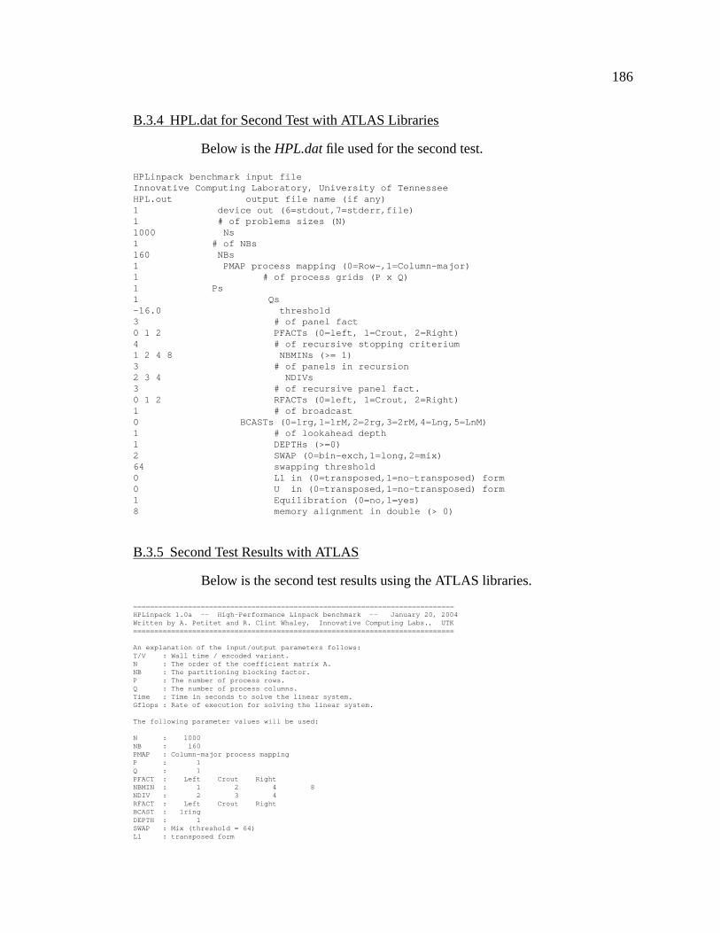
186
B.3.4 HPL.dat for Second Test with ATLAS Libraries
Below is the HPL.dat file used for the second test.
HPLinpack benchmark input fileInnovative Computing Laboratory, University of TennesseeHPL.out output file name (if any)1 device out (6=stdout,7=stderr,file)1 # of problems sizes (N)1000 Ns1 # of NBs160 NBs1 PMAP process mapping (0=Row-,1=Column-major)1 # of process grids (P x Q)1 Ps1 Qs-16.0 threshold3 # of panel fact0 1 2 PFACTs (0=left, 1=Crout, 2=Right)4 # of recursive stopping criterium1 2 4 8 NBMINs (>= 1)3 # of panels in recursion2 3 4 NDIVs3 # of recursive panel fact.0 1 2 RFACTs (0=left, 1=Crout, 2=Right)1 # of broadcast0 BCASTs (0=1rg,1=1rM,2=2rg,3=2rM,4=Lng,5=LnM)1 # of lookahead depth1 DEPTHs (>=0)2 SWAP (0=bin-exch,1=long,2=mix)64 swapping threshold0 L1 in (0=transposed,1=no-transposed) form0 U in (0=transposed,1=no-transposed) form1 Equilibration (0=no,1=yes)8 memory alignment in double (> 0)
B.3.5 Second Test Results with ATLAS
Below is the second test results using the ATLAS libraries.
============================================================================HPLinpack 1.0a -- High-Performance Linpack benchmark -- January 20, 2004Written by A. Petitet and R. Clint Whaley, Innovative Computing Labs., UTK============================================================================
An explanation of the input/output parameters follows:T/V : Wall time / encoded variant.N : The order of the coefficient matrix A.NB : The partitioning blocking factor.P : The number of process rows.Q : The number of process columns.Time : Time in seconds to solve the linear system.Gflops : Rate of execution for solving the linear system.
The following parameter values will be used:
N : 1000NB : 160PMAP : Column-major process mappingP : 1Q : 1PFACT : Left Crout RightNBMIN : 1 2 4 8NDIV : 2 3 4RFACT : Left Crout RightBCAST : 1ringDEPTH : 1SWAP : Mix (threshold = 64)L1 : transposed form
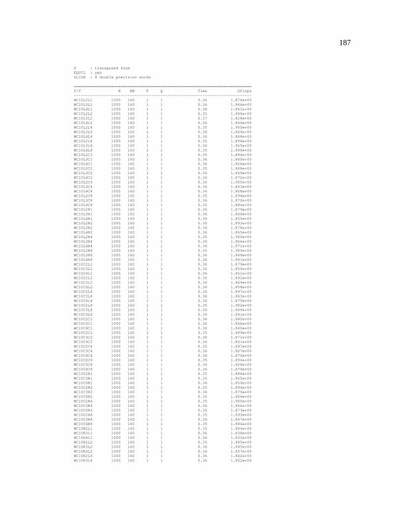
187
U : transposed formEQUIL : yesALIGN : 8 double precision words
============================================================================T/V N NB P Q Time Gflops----------------------------------------------------------------------------WC10L2L1 1000 160 1 1 0.36 1.876e+00WC10L3L1 1000 160 1 1 0.36 1.866e+00WC10L4L1 1000 160 1 1 0.36 1.861e+00WC10L2L2 1000 160 1 1 0.35 1.888e+00WC10L3L2 1000 160 1 1 0.37 1.828e+00WC10L4L2 1000 160 1 1 0.36 1.864e+00WC10L2L4 1000 160 1 1 0.35 1.900e+00WC10L3L4 1000 160 1 1 0.36 1.869e+00WC10L4L4 1000 160 1 1 0.36 1.868e+00WC10L2L8 1000 160 1 1 0.35 1.896e+00WC10L3L8 1000 160 1 1 0.36 1.865e+00WC10L4L8 1000 160 1 1 0.35 1.886e+00WC10L2C1 1000 160 1 1 0.35 1.884e+00WC10L3C1 1000 160 1 1 0.36 1.860e+00WC10L4C1 1000 160 1 1 0.36 1.856e+00WC10L2C2 1000 160 1 1 0.35 1.888e+00WC10L3C2 1000 160 1 1 0.36 1.865e+00WC10L4C2 1000 160 1 1 0.36 1.872e+00WC10L2C4 1000 160 1 1 0.35 1.900e+00WC10L3C4 1000 160 1 1 0.36 1.863e+00WC10L4C4 1000 160 1 1 0.36 1.868e+00WC10L2C8 1000 160 1 1 0.35 1.894e+00WC10L3C8 1000 160 1 1 0.36 1.870e+00WC10L4C8 1000 160 1 1 0.35 1.884e+00WC10L2R1 1000 160 1 1 0.36 1.879e+00WC10L3R1 1000 160 1 1 0.36 1.860e+00WC10L4R1 1000 160 1 1 0.36 1.855e+00WC10L2R2 1000 160 1 1 0.35 1.893e+00WC10L3R2 1000 160 1 1 0.36 1.878e+00WC10L4R2 1000 160 1 1 0.36 1.865e+00WC10L2R4 1000 160 1 1 0.35 1.900e+00WC10L3R4 1000 160 1 1 0.36 1.866e+00WC10L4R4 1000 160 1 1 0.36 1.871e+00WC10L2R8 1000 160 1 1 0.35 1.900e+00WC10L3R8 1000 160 1 1 0.36 1.869e+00WC10L4R8 1000 160 1 1 0.36 1.881e+00WC10C2L1 1000 160 1 1 0.36 1.879e+00WC10C3L1 1000 160 1 1 0.36 1.859e+00WC10C4L1 1000 160 1 1 0.36 1.852e+00WC10C2L2 1000 160 1 1 0.35 1.892e+00WC10C3L2 1000 160 1 1 0.36 1.869e+00WC10C4L2 1000 160 1 1 0.36 1.858e+00WC10C2L4 1000 160 1 1 0.35 1.897e+00WC10C3L4 1000 160 1 1 0.36 1.863e+00WC10C4L4 1000 160 1 1 0.36 1.875e+00WC10C2L8 1000 160 1 1 0.35 1.902e+00WC10C3L8 1000 160 1 1 0.36 1.869e+00WC10C4L8 1000 160 1 1 0.36 1.881e+00WC10C2C1 1000 160 1 1 0.36 1.880e+00WC10C3C1 1000 160 1 1 0.36 1.866e+00WC10C4C1 1000 160 1 1 0.36 1.860e+00WC10C2C2 1000 160 1 1 0.35 1.889e+00WC10C3C2 1000 160 1 1 0.36 1.871e+00WC10C4C2 1000 160 1 1 0.36 1.861e+00WC10C2C4 1000 160 1 1 0.35 1.897e+00WC10C3C4 1000 160 1 1 0.36 1.867e+00WC10C4C4 1000 160 1 1 0.36 1.870e+00WC10C2C8 1000 160 1 1 0.35 1.894e+00WC10C3C8 1000 160 1 1 0.36 1.868e+00WC10C4C8 1000 160 1 1 0.36 1.879e+00WC10C2R1 1000 160 1 1 0.35 1.886e+00WC10C3R1 1000 160 1 1 0.36 1.865e+00WC10C4R1 1000 160 1 1 0.36 1.854e+00WC10C2R2 1000 160 1 1 0.35 1.894e+00WC10C3R2 1000 160 1 1 0.36 1.875e+00WC10C4R2 1000 160 1 1 0.36 1.864e+00WC10C2R4 1000 160 1 1 0.35 1.905e+00WC10C3R4 1000 160 1 1 0.36 1.866e+00WC10C4R4 1000 160 1 1 0.36 1.873e+00WC10C2R8 1000 160 1 1 0.35 1.893e+00WC10C3R8 1000 160 1 1 0.36 1.867e+00WC10C4R8 1000 160 1 1 0.35 1.884e+00WC10R2L1 1000 160 1 1 0.35 1.884e+00WC10R3L1 1000 160 1 1 0.36 1.838e+00WC10R4L1 1000 160 1 1 0.36 1.832e+00WC10R2L2 1000 160 1 1 0.35 1.885e+00WC10R3L2 1000 160 1 1 0.36 1.845e+00WC10R4L2 1000 160 1 1 0.36 1.857e+00WC10R2L4 1000 160 1 1 0.36 1.862e+00WC10R3L4 1000 160 1 1 0.36 1.852e+00
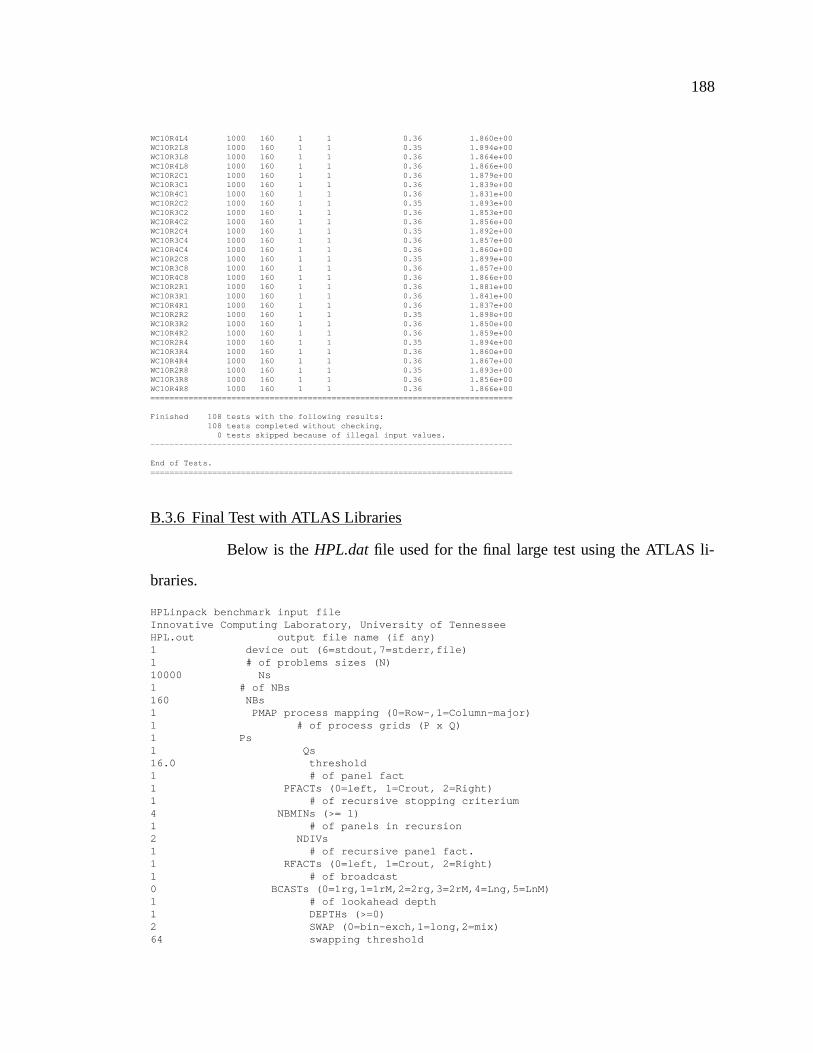
188
WC10R4L4 1000 160 1 1 0.36 1.860e+00WC10R2L8 1000 160 1 1 0.35 1.894e+00WC10R3L8 1000 160 1 1 0.36 1.864e+00WC10R4L8 1000 160 1 1 0.36 1.866e+00WC10R2C1 1000 160 1 1 0.36 1.879e+00WC10R3C1 1000 160 1 1 0.36 1.839e+00WC10R4C1 1000 160 1 1 0.36 1.831e+00WC10R2C2 1000 160 1 1 0.35 1.893e+00WC10R3C2 1000 160 1 1 0.36 1.853e+00WC10R4C2 1000 160 1 1 0.36 1.856e+00WC10R2C4 1000 160 1 1 0.35 1.892e+00WC10R3C4 1000 160 1 1 0.36 1.857e+00WC10R4C4 1000 160 1 1 0.36 1.860e+00WC10R2C8 1000 160 1 1 0.35 1.899e+00WC10R3C8 1000 160 1 1 0.36 1.857e+00WC10R4C8 1000 160 1 1 0.36 1.866e+00WC10R2R1 1000 160 1 1 0.36 1.881e+00WC10R3R1 1000 160 1 1 0.36 1.841e+00WC10R4R1 1000 160 1 1 0.36 1.837e+00WC10R2R2 1000 160 1 1 0.35 1.898e+00WC10R3R2 1000 160 1 1 0.36 1.850e+00WC10R4R2 1000 160 1 1 0.36 1.859e+00WC10R2R4 1000 160 1 1 0.35 1.894e+00WC10R3R4 1000 160 1 1 0.36 1.860e+00WC10R4R4 1000 160 1 1 0.36 1.867e+00WC10R2R8 1000 160 1 1 0.35 1.893e+00WC10R3R8 1000 160 1 1 0.36 1.856e+00WC10R4R8 1000 160 1 1 0.36 1.866e+00============================================================================
Finished 108 tests with the following results:108 tests completed without checking,0 tests skipped because of illegal input values.
----------------------------------------------------------------------------
End of Tests.============================================================================
B.3.6 Final Test with ATLAS Libraries
Below is the HPL.dat file used for the final large test using the ATLAS li-
braries.
HPLinpack benchmark input fileInnovative Computing Laboratory, University of TennesseeHPL.out output file name (if any)1 device out (6=stdout,7=stderr,file)1 # of problems sizes (N)10000 Ns1 # of NBs160 NBs1 PMAP process mapping (0=Row-,1=Column-major)1 # of process grids (P x Q)1 Ps1 Qs16.0 threshold1 # of panel fact1 PFACTs (0=left, 1=Crout, 2=Right)1 # of recursive stopping criterium4 NBMINs (>= 1)1 # of panels in recursion2 NDIVs1 # of recursive panel fact.1 RFACTs (0=left, 1=Crout, 2=Right)1 # of broadcast0 BCASTs (0=1rg,1=1rM,2=2rg,3=2rM,4=Lng,5=LnM)1 # of lookahead depth1 DEPTHs (>=0)2 SWAP (0=bin-exch,1=long,2=mix)64 swapping threshold
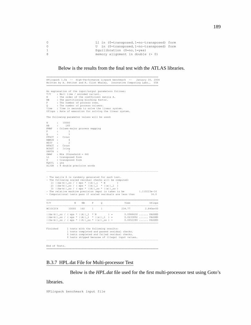
189
0 L1 in (0=transposed,1=no-transposed) form0 U in (0=transposed,1=no-transposed) form1 Equilibration (0=no,1=yes)8 memory alignment in double (> 0)
Below is the results from the final test with the ATLAS libraries.
============================================================================HPLinpack 1.0a -- High-Performance Linpack benchmark -- January 20, 2004Written by A. Petitet and R. Clint Whaley, Innovative Computing Labs., UTK============================================================================
An explanation of the input/output parameters follows:T/V : Wall time / encoded variant.N : The order of the coefficient matrix A.NB : The partitioning blocking factor.P : The number of process rows.Q : The number of process columns.Time : Time in seconds to solve the linear system.Gflops : Rate of execution for solving the linear system.
The following parameter values will be used:
N : 10000NB : 160PMAP : Column-major process mappingP : 1Q : 1PFACT : CroutNBMIN : 4NDIV : 2RFACT : CroutBCAST : 1ringDEPTH : 1SWAP : Mix (threshold = 64)L1 : transposed formU : transposed formEQUIL : yesALIGN : 8 double precision words
----------------------------------------------------------------------------
- The matrix A is randomly generated for each test.- The following scaled residual checks will be computed:
1) ||Ax-b||_oo / ( eps * ||A||_1 * N )2) ||Ax-b||_oo / ( eps * ||A||_1 * ||x||_1 )3) ||Ax-b||_oo / ( eps * ||A||_oo * ||x||_oo )
- The relative machine precision (eps) is taken to be 1.110223e-16- Computational tests pass if scaled residuals are less than 16.0
============================================================================T/V N NB P Q Time Gflops----------------------------------------------------------------------------WC10C2C4 10000 160 1 1 234.77 2.840e+00----------------------------------------------------------------------------||Ax-b||_oo / ( eps * ||A||_1 * N ) = 0.0988430 ...... PASSED||Ax-b||_oo / ( eps * ||A||_1 * ||x||_1 ) = 0.0233892 ...... PASSED||Ax-b||_oo / ( eps * ||A||_oo * ||x||_oo ) = 0.0052280 ...... PASSED============================================================================
Finished 1 tests with the following results:1 tests completed and passed residual checks,0 tests completed and failed residual checks,0 tests skipped because of illegal input values.
----------------------------------------------------------------------------
End of Tests.============================================================================
B.3.7 HPL.dat File for Multi-processor Test
Below is the HPL.dat file used for the first multi-processor test using Goto’s
libraries.
HPLinpack benchmark input file
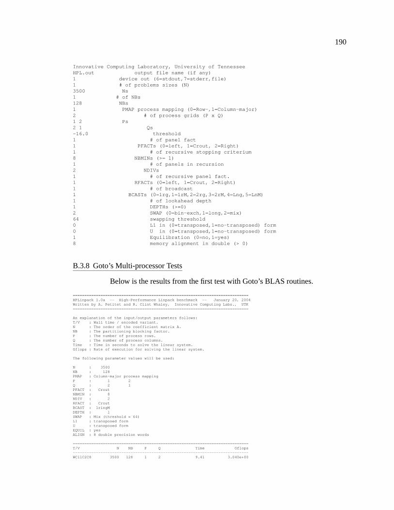
190
Innovative Computing Laboratory, University of TennesseeHPL.out output file name (if any)1 device out (6=stdout,7=stderr,file)1 # of problems sizes (N)3500 Ns1 # of NBs128 NBs1 PMAP process mapping (0=Row-,1=Column-major)2 # of process grids (P x Q)1 2 Ps2 1 Qs-16.0 threshold1 # of panel fact1 PFACTs (0=left, 1=Crout, 2=Right)1 # of recursive stopping criterium8 NBMINs (>= 1)1 # of panels in recursion2 NDIVs1 # of recursive panel fact.1 RFACTs (0=left, 1=Crout, 2=Right)1 # of broadcast1 BCASTs (0=1rg,1=1rM,2=2rg,3=2rM,4=Lng,5=LnM)1 # of lookahead depth1 DEPTHs (>=0)2 SWAP (0=bin-exch,1=long,2=mix)64 swapping threshold0 L1 in (0=transposed,1=no-transposed) form0 U in (0=transposed,1=no-transposed) form1 Equilibration (0=no,1=yes)8 memory alignment in double (> 0)
B.3.8 Goto’s Multi-processor Tests
Below is the results from the first test with Goto’s BLAS routines.
============================================================================HPLinpack 1.0a -- High-Performance Linpack benchmark -- January 20, 2004Written by A. Petitet and R. Clint Whaley, Innovative Computing Labs., UTK============================================================================
An explanation of the input/output parameters follows:T/V : Wall time / encoded variant.N : The order of the coefficient matrix A.NB : The partitioning blocking factor.P : The number of process rows.Q : The number of process columns.Time : Time in seconds to solve the linear system.Gflops : Rate of execution for solving the linear system.
The following parameter values will be used:
N : 3500NB : 128PMAP : Column-major process mappingP : 1 2Q : 2 1PFACT : CroutNBMIN : 8NDIV : 2RFACT : CroutBCAST : 1ringMDEPTH : 1SWAP : Mix (threshold = 64)L1 : transposed formU : transposed formEQUIL : yesALIGN : 8 double precision words
============================================================================T/V N NB P Q Time Gflops----------------------------------------------------------------------------WC11C2C8 3500 128 1 2 9.41 3.040e+00
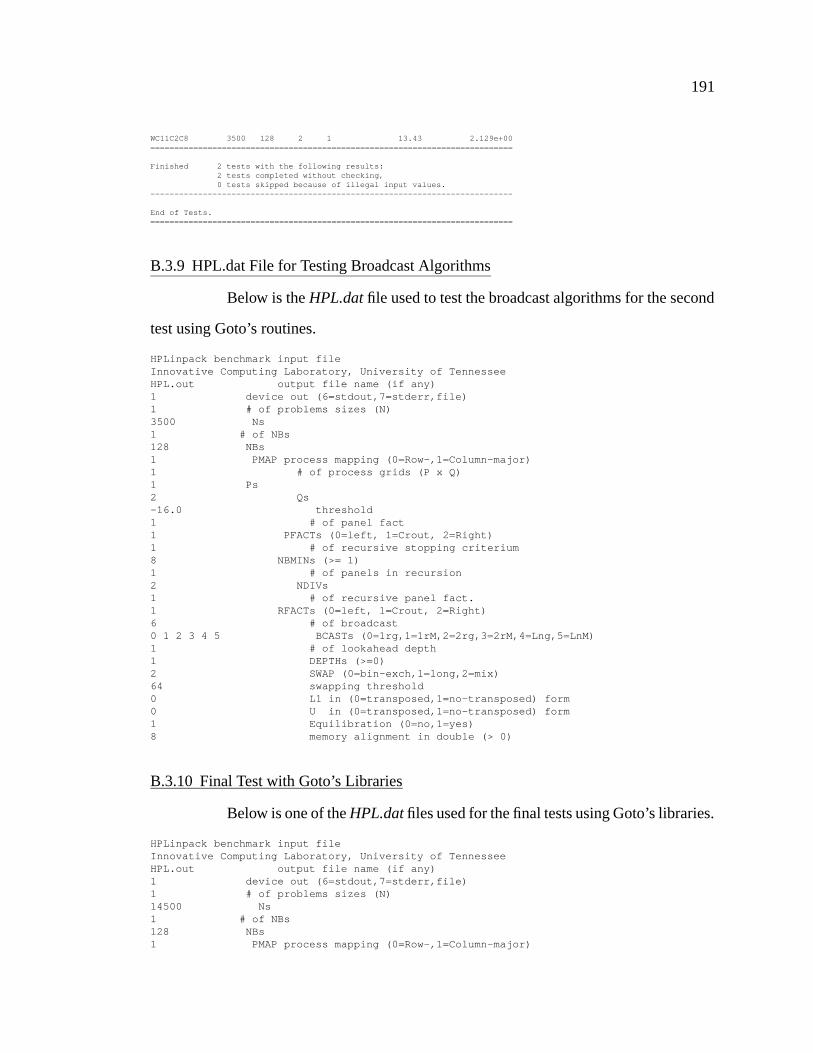
191
WC11C2C8 3500 128 2 1 13.43 2.129e+00============================================================================
Finished 2 tests with the following results:2 tests completed without checking,0 tests skipped because of illegal input values.
----------------------------------------------------------------------------
End of Tests.============================================================================
B.3.9 HPL.dat File for Testing Broadcast Algorithms
Below is the HPL.dat file used to test the broadcast algorithms for the second
test using Goto’s routines.
HPLinpack benchmark input fileInnovative Computing Laboratory, University of TennesseeHPL.out output file name (if any)1 device out (6=stdout,7=stderr,file)1 # of problems sizes (N)3500 Ns1 # of NBs128 NBs1 PMAP process mapping (0=Row-,1=Column-major)1 # of process grids (P x Q)1 Ps2 Qs-16.0 threshold1 # of panel fact1 PFACTs (0=left, 1=Crout, 2=Right)1 # of recursive stopping criterium8 NBMINs (>= 1)1 # of panels in recursion2 NDIVs1 # of recursive panel fact.1 RFACTs (0=left, 1=Crout, 2=Right)6 # of broadcast0 1 2 3 4 5 BCASTs (0=1rg,1=1rM,2=2rg,3=2rM,4=Lng,5=LnM)1 # of lookahead depth1 DEPTHs (>=0)2 SWAP (0=bin-exch,1=long,2=mix)64 swapping threshold0 L1 in (0=transposed,1=no-transposed) form0 U in (0=transposed,1=no-transposed) form1 Equilibration (0=no,1=yes)8 memory alignment in double (> 0)
B.3.10 Final Test with Goto’s Libraries
Below is one of the HPL.dat files used for the final tests using Goto’s libraries.
HPLinpack benchmark input fileInnovative Computing Laboratory, University of TennesseeHPL.out output file name (if any)1 device out (6=stdout,7=stderr,file)1 # of problems sizes (N)14500 Ns1 # of NBs128 NBs1 PMAP process mapping (0=Row-,1=Column-major)
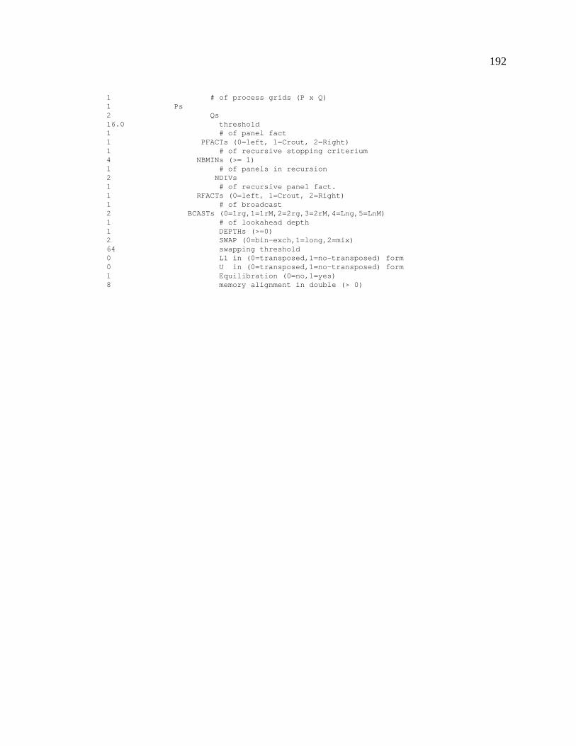
192
1 # of process grids (P x Q)1 Ps2 Qs16.0 threshold1 # of panel fact1 PFACTs (0=left, 1=Crout, 2=Right)1 # of recursive stopping criterium4 NBMINs (>= 1)1 # of panels in recursion2 NDIVs1 # of recursive panel fact.1 RFACTs (0=left, 1=Crout, 2=Right)1 # of broadcast2 BCASTs (0=1rg,1=1rM,2=2rg,3=2rM,4=Lng,5=LnM)1 # of lookahead depth1 DEPTHs (>=0)2 SWAP (0=bin-exch,1=long,2=mix)64 swapping threshold0 L1 in (0=transposed,1=no-transposed) form0 U in (0=transposed,1=no-transposed) form1 Equilibration (0=no,1=yes)8 memory alignment in double (> 0)
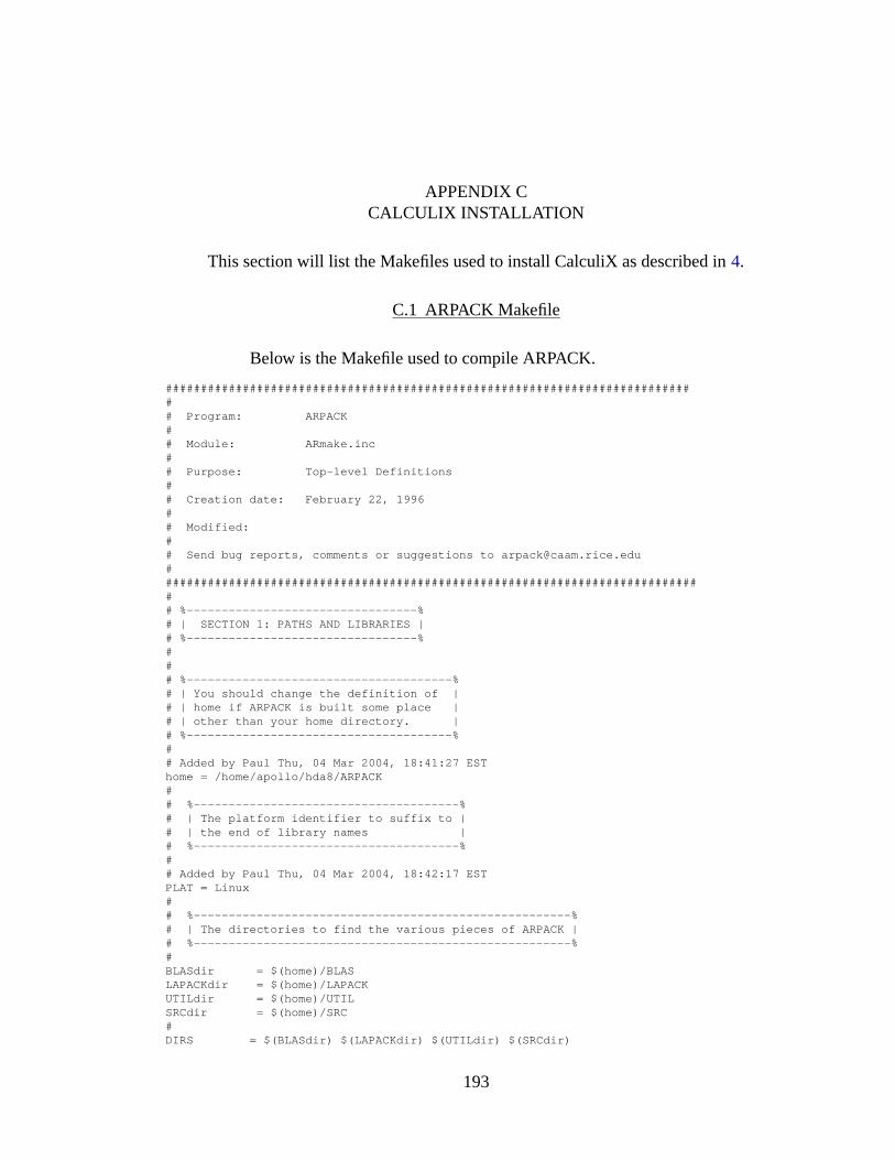
APPENDIX CCALCULIX INSTALLATION
This section will list the Makefiles used to install CalculiX as described in 4.
C.1 ARPACK Makefile
Below is the Makefile used to compile ARPACK.
############################################################################# Program: ARPACK## Module: ARmake.inc## Purpose: Top-level Definitions## Creation date: February 22, 1996## Modified:## Send bug reports, comments or suggestions to [email protected]############################################################################### %---------------------------------%# | SECTION 1: PATHS AND LIBRARIES |# %---------------------------------%### %--------------------------------------%# | You should change the definition of |# | home if ARPACK is built some place |# | other than your home directory. |# %--------------------------------------%## Added by Paul Thu, 04 Mar 2004, 18:41:27 ESThome = /home/apollo/hda8/ARPACK## %--------------------------------------%# | The platform identifier to suffix to |# | the end of library names |# %--------------------------------------%## Added by Paul Thu, 04 Mar 2004, 18:42:17 ESTPLAT = Linux## %------------------------------------------------------%# | The directories to find the various pieces of ARPACK |# %------------------------------------------------------%#BLASdir = $(home)/BLASLAPACKdir = $(home)/LAPACKUTILdir = $(home)/UTILSRCdir = $(home)/SRC#DIRS = $(BLASdir) $(LAPACKdir) $(UTILdir) $(SRCdir)
193
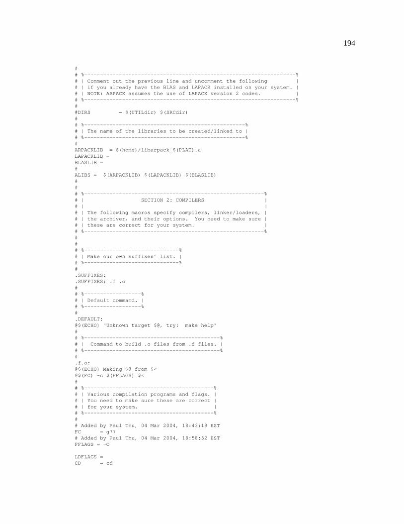
194
## %-------------------------------------------------------------------%# | Comment out the previous line and uncomment the following |# | if you already have the BLAS and LAPACK installed on your system. |# | NOTE: ARPACK assumes the use of LAPACK version 2 codes. |# %-------------------------------------------------------------------%##DIRS = $(UTILdir) $(SRCdir)## %---------------------------------------------------%# | The name of the libraries to be created/linked to |# %---------------------------------------------------%#ARPACKLIB = $(home)/libarpack_$(PLAT).aLAPACKLIB =BLASLIB =#ALIBS = $(ARPACKLIB) $(LAPACKLIB) $(BLASLIB)### %---------------------------------------------------------%# | SECTION 2: COMPILERS |# | |# | The following macros specify compilers, linker/loaders, |# | the archiver, and their options. You need to make sure |# | these are correct for your system. |# %---------------------------------------------------------%### %------------------------------%# | Make our own suffixes’ list. |# %------------------------------%#.SUFFIXES:.SUFFIXES: .f .o## %------------------%# | Default command. |# %------------------%#.DEFAULT:@$(ECHO) "Unknown target $@, try: make help"## %-------------------------------------------%# | Command to build .o files from .f files. |# %-------------------------------------------%#.f.o:@$(ECHO) Making $@ from $<@$(FC) -c $(FFLAGS) $<## %-----------------------------------------%# | Various compilation programs and flags. |# | You need to make sure these are correct |# | for your system. |# %-----------------------------------------%## Added by Paul Thu, 04 Mar 2004, 18:43:19 ESTFC = g77# Added by Paul Thu, 04 Mar 2004, 18:58:52 ESTFFLAGS = -O
LDFLAGS =CD = cd
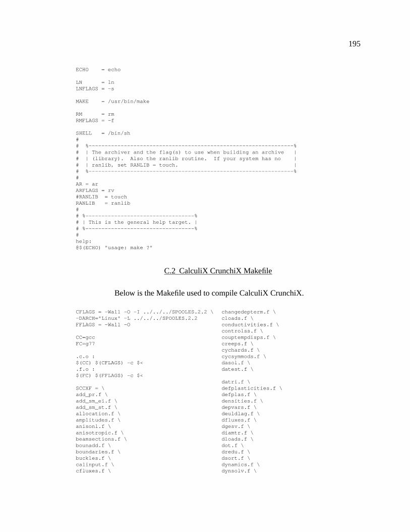
195
ECHO = echo
LN = lnLNFLAGS = -s
MAKE = /usr/bin/make
RM = rmRMFLAGS = -f
SHELL = /bin/sh## %----------------------------------------------------------------%# | The archiver and the flag(s) to use when building an archive |# | (library). Also the ranlib routine. If your system has no |# | ranlib, set RANLIB = touch. |# %----------------------------------------------------------------%#AR = arARFLAGS = rv#RANLIB = touchRANLIB = ranlib## %----------------------------------%# | This is the general help target. |# %----------------------------------%#help:@$(ECHO) "usage: make ?"
C.2 CalculiX CrunchiX Makefile
Below is the Makefile used to compile CalculiX CrunchiX.
CFLAGS = -Wall -O -I ../../../SPOOLES.2.2 \-DARCH="Linux" -L ../../../SPOOLES.2.2FFLAGS = -Wall -O
CC=gccFC=g77
.c.o :$(CC) $(CFLAGS) -c $<.f.o :$(FC) $(FFLAGS) -c $<
SCCXF = \add_pr.f \add_sm_ei.f \add_sm_st.f \allocation.f \amplitudes.f \anisonl.f \anisotropic.f \beamsections.f \bounadd.f \boundaries.f \buckles.f \calinput.f \cfluxes.f \
changedepterm.f \cloads.f \conductivities.f \controlss.f \couptempdisps.f \creeps.f \cychards.f \cycsymmods.f \dasol.f \datest.f \
datri.f \defplasticities.f \defplas.f \densities.f \depvars.f \deuldlag.f \dfluxes.f \dgesv.f \diamtr.f \dloads.f \dot.f \dredu.f \dsort.f \dynamics.f \dynsolv.f \
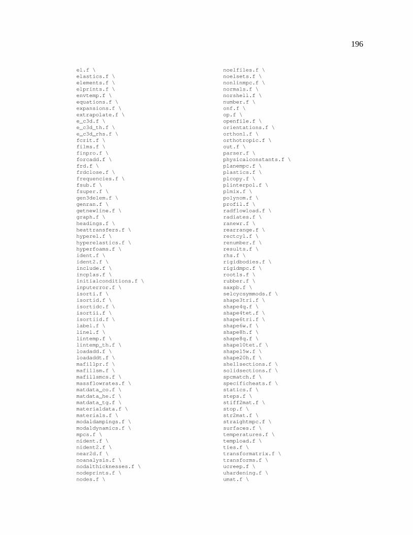
196
el.f \elastics.f \elements.f \elprints.f \envtemp.f \equations.f \expansions.f \extrapolate.f \e_c3d.f \e_c3d_th.f \e_c3d_rhs.f \fcrit.f \films.f \finpro.f \forcadd.f \frd.f \frdclose.f \frequencies.f \fsub.f \fsuper.f \gen3delem.f \genran.f \getnewline.f \graph.f \headings.f \heattransfers.f \hyperel.f \hyperelastics.f \hyperfoams.f \ident.f \ident2.f \include.f \incplas.f \initialconditions.f \inputerror.f \isorti.f \isortid.f \isortidc.f \isortii.f \isortiid.f \label.f \linel.f \lintemp.f \lintemp_th.f \loadadd.f \loadaddt.f \mafillpr.f \mafillsm.f \mafillsmcs.f \massflowrates.f \matdata_co.f \matdata_he.f \matdata_tg.f \materialdata.f \materials.f \modaldampings.f \modaldynamics.f \mpcs.f \nident.f \nident2.f \near2d.f \noanalysis.f \nodalthicknesses.f \nodeprints.f \nodes.f \
noelfiles.f \noelsets.f \nonlinmpc.f \normals.f \norshell.f \number.f \onf.f \op.f \openfile.f \orientations.f \orthonl.f \orthotropic.f \out.f \parser.f \physicalconstants.f \planempc.f \plastics.f \plcopy.f \plinterpol.f \plmix.f \polynom.f \profil.f \radflowload.f \radiates.f \ranewr.f \rearrange.f \rectcyl.f \renumber.f \results.f \rhs.f \rigidbodies.f \rigidmpc.f \rootls.f \rubber.f \saxpb.f \selcycsymmods.f \shape3tri.f \shape4q.f \shape4tet.f \shape6tri.f \shape6w.f \shape8h.f \shape8q.f \shape10tet.f \shape15w.f \shape20h.f \shellsections.f \solidsections.f \spcmatch.f \specificheats.f \statics.f \steps.f \stiff2mat.f \stop.f \str2mat.f \straightmpc.f \surfaces.f \temperatures.f \tempload.f \ties.f \transformatrix.f \transforms.f \ucreep.f \uhardening.f \umat.f \
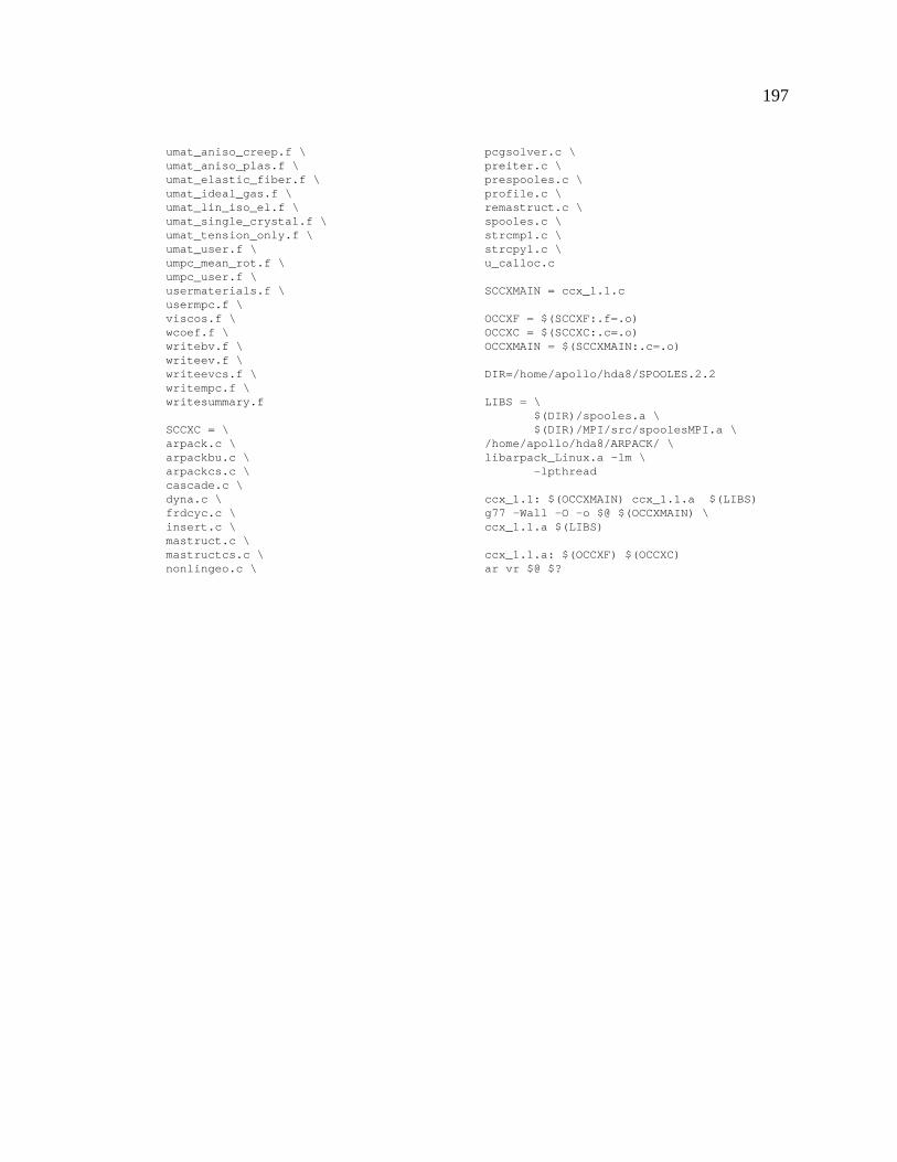
197
umat_aniso_creep.f \umat_aniso_plas.f \umat_elastic_fiber.f \umat_ideal_gas.f \umat_lin_iso_el.f \umat_single_crystal.f \umat_tension_only.f \umat_user.f \umpc_mean_rot.f \umpc_user.f \usermaterials.f \usermpc.f \viscos.f \wcoef.f \writebv.f \writeev.f \writeevcs.f \writempc.f \writesummary.f
SCCXC = \arpack.c \arpackbu.c \arpackcs.c \cascade.c \dyna.c \frdcyc.c \insert.c \mastruct.c \mastructcs.c \nonlingeo.c \
pcgsolver.c \preiter.c \prespooles.c \profile.c \remastruct.c \spooles.c \strcmp1.c \strcpy1.c \u_calloc.c
SCCXMAIN = ccx_1.1.c
OCCXF = $(SCCXF:.f=.o)OCCXC = $(SCCXC:.c=.o)OCCXMAIN = $(SCCXMAIN:.c=.o)
DIR=/home/apollo/hda8/SPOOLES.2.2
LIBS = \$(DIR)/spooles.a \$(DIR)/MPI/src/spoolesMPI.a \
/home/apollo/hda8/ARPACK/ \libarpack_Linux.a -lm \
-lpthread
ccx_1.1: $(OCCXMAIN) ccx_1.1.a $(LIBS)g77 -Wall -O -o $@ $(OCCXMAIN) \ccx_1.1.a $(LIBS)
ccx_1.1.a: $(OCCXF) $(OCCXC)ar vr $@ $?
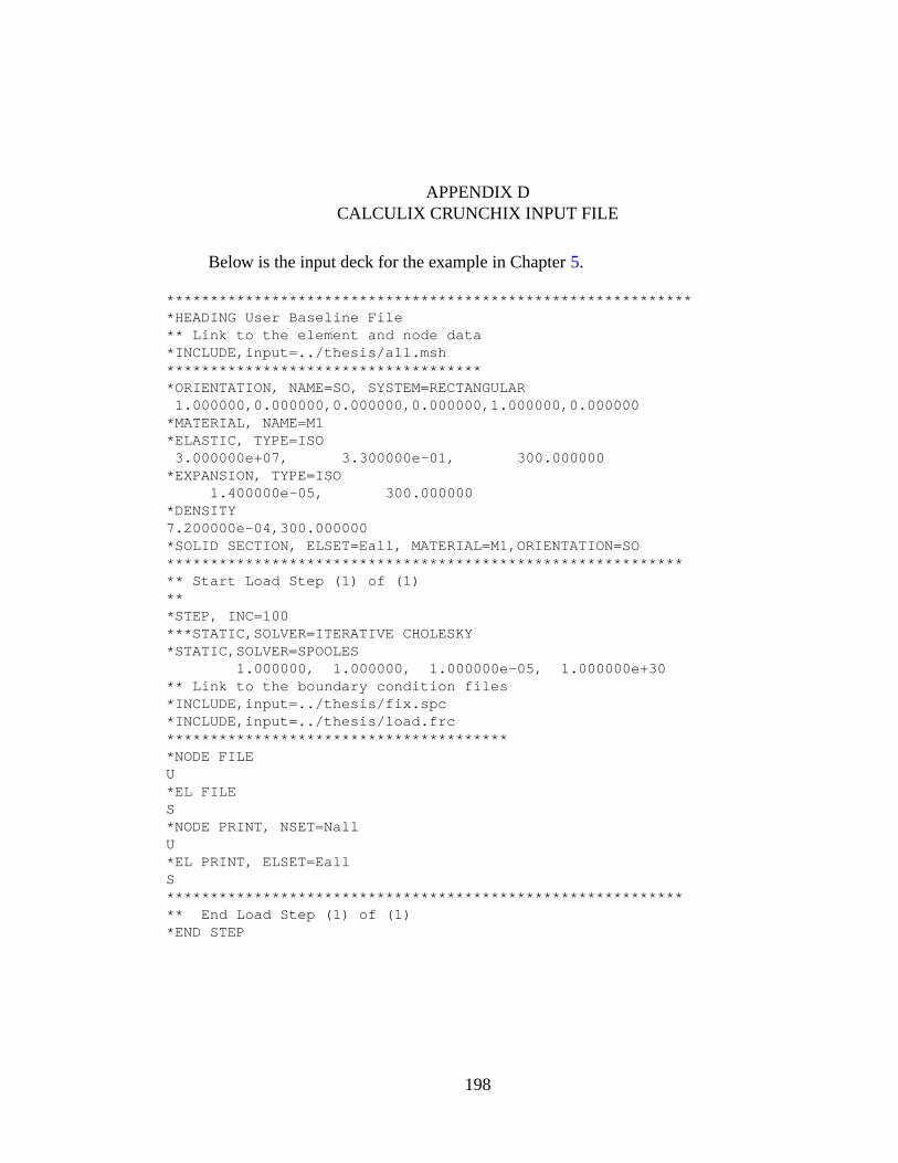
APPENDIX DCALCULIX CRUNCHIX INPUT FILE
Below is the input deck for the example in Chapter 5.
*************************************************************HEADING User Baseline File** Link to the element and node data*INCLUDE,input=../thesis/all.msh*************************************ORIENTATION, NAME=SO, SYSTEM=RECTANGULAR1.000000,0.000000,0.000000,0.000000,1.000000,0.000000*MATERIAL, NAME=M1*ELASTIC, TYPE=ISO3.000000e+07, 3.300000e-01, 300.000000*EXPANSION, TYPE=ISO
1.400000e-05, 300.000000*DENSITY7.200000e-04,300.000000*SOLID SECTION, ELSET=Eall, MATERIAL=M1,ORIENTATION=SO************************************************************* Start Load Step (1) of (1)***STEP, INC=100***STATIC,SOLVER=ITERATIVE CHOLESKY*STATIC,SOLVER=SPOOLES
1.000000, 1.000000, 1.000000e-05, 1.000000e+30** Link to the boundary condition files*INCLUDE,input=../thesis/fix.spc*INCLUDE,input=../thesis/load.frc****************************************NODE FILEU*EL FILES*NODE PRINT, NSET=NallU*EL PRINT, ELSET=EallS************************************************************* End Load Step (1) of (1)*END STEP
198

APPENDIX ESERIAL AND PARALLEL SOLVER SOURCE CODE
The below sections will display the source code for both the serial and parallel
solvers. The serial code will be the original supplied by CalculiX while the parallel code
will be the final optimized program.
E.1 Serial Code
Below is the source code for the serial solver of CalculiX CrunchiX.
/* CalculiX - A 3-dimensional finite element program *//* Copyright (C) 1998 Guido Dhondt */
/* This program is free software; you can redistribute it and/or *//* modify it under the terms of the GNU General Public License as *//* published by the Free Software Foundation(version 2); *//* */
/* This program is distributed in the hope that it will be useful, *//* but WITHOUT ANY WARRANTY; without even the implied warranty of *//* MERCHANTABILITY or FITNESS FOR A PARTICULAR PURPOSE. See the *//* GNU General Public License for more details. */
/* You should have received a copy of the GNU General Public License *//* along with this program; if not, write to the Free Software *//* Foundation, Inc., 675 Mass Ave, Cambridge, MA 02139, USA. */
#include <stdio.h>#include <sys/types.h>#include <time.h>#include <math.h>#include <stdlib.h>#include <misc.h>#include <FrontMtx.h>#include <SymbFac.h>#include "CalculiX.h"
void spooles(double *ad, double *au, double *b, int *icol, int *irow,int *neq, int *nzs){
char buffer[20];int ipoint,ipo;DenseMtx *mtxB, *mtxX ;Chv *rootchv ;
199
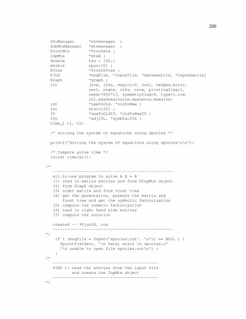
200
ChvManager *chvmanager ;SubMtxManager *mtxmanager ;FrontMtx *frontmtx ;InpMtx *mtxA ;double tau = 100.;double cpus[10] ;ETree *frontETree ;FILE *msgFile, *inputFile, *densematrix, *inputmatrix;Graph *graph ;int jrow, jrhs, msglvl=0, ncol, nedges,error,
nent, neqns, nrhs, nrow, pivotingflag=1,seed=7892713, symmetryflag=0, type=1,row,col,maxdomainsize,maxzeros,maxsize;
int *newToOld, *oldToNew ;int stats[20] ;IV *newToOldIV, *oldToNewIV ;IVL *adjIVL, *symbfacIVL ;time_t t1, t2;
/* solving the system of equations using spooles */
printf("Solving the system of equations using spooles\n\n");
/* Compute solve time */(void) time(&t1);
/*--------------------------------------------------all-in-one program to solve A X = B(1) read in matrix entries and form DInpMtx object(2) form Graph object(3) order matrix and form front tree(4) get the permutation, permute the matrix and
front tree and get the symbolic factorization(5) compute the numeric factorization(6) read in right hand side entries(7) compute the solution
created -- 98jun04, cca--------------------------------------------------
*/if ( (msgFile = fopen("spooles.out", "a")) == NULL ) {fprintf(stderr, "\n fatal error in spooles.c""\n unable to open file spooles.out\n") ;
}/*
--------------------------------------------STEP 1: read the entries from the input file
and create the InpMtx object--------------------------------------------
*/
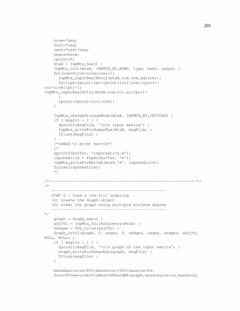
201
nrow=*neq;ncol=*neq;nent=*nzs+*neq;neqns=nrow;ipoint=0;mtxA = InpMtx_new() ;InpMtx_init(mtxA, INPMTX_BY_ROWS, type, nent, neqns) ;for(row=0;row<nrow;row++){InpMtx_inputRealEntry(mtxA,row,row,ad[row]);for(ipo=ipoint;ipo<ipoint+icol[row];ipo++){
col=irow[ipo]-1;InpMtx_inputRealEntry(mtxA,row,col,au[ipo]);
}ipoint=ipoint+icol[row];
}
InpMtx_changeStorageMode(mtxA, INPMTX_BY_VECTORS) ;if ( msglvl > 1 ) {fprintf(msgFile, "\n\n input matrix") ;InpMtx_writeForHumanEye(mtxA, msgFile) ;fflush(msgFile) ;
}/*added to print matrix*//*sprintf(buffer, "inputmatrix.m");inputmatrix = fopen(buffer, "w");InpMtx_writeForMatlab(mtxA,"A", inputmatrix);fclose(inputmatrix);*/
/*---------------------------------------------------------------*//*
-------------------------------------------------STEP 2 : find a low-fill ordering(1) create the Graph object(2) order the graph using multiple minimum degree-------------------------------------------------
*/graph = Graph_new() ;adjIVL = InpMtx_fullAdjacency(mtxA) ;nedges = IVL_tsize(adjIVL) ;Graph_init2(graph, 0, neqns, 0, nedges, neqns, nedges, adjIVL,
NULL, NULL) ;if ( msglvl > 1 ) {fprintf(msgFile, "\n\n graph of the input matrix") ;Graph_writeForHumanEye(graph, msgFile) ;fflush(msgFile) ;
}
maxdomainsize=800;maxzeros=1000;maxsize=64;frontETree=orderViaBestOfNDandMS(graph,maxdomainsize,maxzeros,
202
maxsize,seed,msglvl,msgFile);if ( msglvl > 1 ) {fprintf(msgFile, "\n\n front tree from ordering") ;ETree_writeForHumanEye(frontETree, msgFile) ;fflush(msgFile) ;
}/*---------------------------------------------------------------*//*
-----------------------------------------------------STEP 3: get the permutation, permute the matrix and
front tree and get the symbolic factorization-----------------------------------------------------
*/oldToNewIV = ETree_oldToNewVtxPerm(frontETree) ;oldToNew = IV_entries(oldToNewIV) ;newToOldIV = ETree_newToOldVtxPerm(frontETree) ;newToOld = IV_entries(newToOldIV) ;ETree_permuteVertices(frontETree, oldToNewIV) ;InpMtx_permute(mtxA, oldToNew, oldToNew) ;InpMtx_mapToUpperTriangle(mtxA) ;InpMtx_changeCoordType(mtxA,INPMTX_BY_CHEVRONS);InpMtx_changeStorageMode(mtxA,INPMTX_BY_VECTORS);symbfacIVL = SymbFac_initFromInpMtx(frontETree, mtxA) ;if ( msglvl > 1 ) {fprintf(msgFile, "\n\n old-to-new permutation vector") ;IV_writeForHumanEye(oldToNewIV, msgFile) ;fprintf(msgFile, "\n\n new-to-old permutation vector") ;IV_writeForHumanEye(newToOldIV, msgFile) ;fprintf(msgFile, "\n\n front tree after permutation") ;ETree_writeForHumanEye(frontETree, msgFile) ;fprintf(msgFile, "\n\n input matrix after permutation") ;InpMtx_writeForHumanEye(mtxA, msgFile) ;fprintf(msgFile, "\n\n symbolic factorization") ;IVL_writeForHumanEye(symbfacIVL, msgFile) ;fflush(msgFile) ;
}/*---------------------------------------------------------------*//*
------------------------------------------STEP 4: initialize the front matrix object------------------------------------------
*/frontmtx = FrontMtx_new() ;mtxmanager = SubMtxManager_new() ;SubMtxManager_init(mtxmanager, NO_LOCK, 0) ;FrontMtx_init(frontmtx, frontETree, symbfacIVL, type,
symmetryflag,FRONTMTX_DENSE_FRONTS, pivotingflag, NO_LOCK, 0, NULL,mtxmanager, msglvl, msgFile) ;
/*---------------------------------------------------------------*//*
203
-----------------------------------------STEP 5: compute the numeric factorization-----------------------------------------
*/chvmanager = ChvManager_new() ;ChvManager_init(chvmanager, NO_LOCK, 1) ;DVfill(10, cpus, 0.0) ;IVfill(20, stats, 0) ;rootchv = FrontMtx_factorInpMtx(frontmtx, mtxA, tau, 0.0,
chvmanager,&error,cpus, stats, msglvl, msgFile) ;ChvManager_free(chvmanager) ;if ( msglvl > 1 ) {fprintf(msgFile, "\n\n factor matrix") ;FrontMtx_writeForHumanEye(frontmtx, msgFile) ;fflush(msgFile) ;
}if ( rootchv != NULL ) {fprintf(msgFile, "\n\n matrix found to be singular\n") ;exit(-1) ;
}if(error>=0){fprintf(msgFile,"\n\nerror encountered at front %d",error);exit(-1);
}/*---------------------------------------------------------------*//*
--------------------------------------STEP 6: post-process the factorization--------------------------------------
*/FrontMtx_postProcess(frontmtx, msglvl, msgFile) ;if ( msglvl > 1 ) {fprintf(msgFile, "\n\n factor matrix after post-processing") ;FrontMtx_writeForHumanEye(frontmtx, msgFile) ;fflush(msgFile) ;
}/*---------------------------------------------------------------*//*
-----------------------------------------STEP 7: read the right hand side matrix B-----------------------------------------
*/nrhs=1;mtxB = DenseMtx_new() ;DenseMtx_init(mtxB, type, 0, 0, neqns, nrhs, 1, neqns) ;DenseMtx_zero(mtxB) ;for ( jrow = 0 ; jrow < nrow ; jrow++ ) {for ( jrhs = 0 ; jrhs < nrhs ; jrhs++ ) {
DenseMtx_setRealEntry(mtxB, jrow, jrhs, b[jrow]) ;}
204
}
if ( msglvl > 1 ) {fprintf(msgFile, "\n\n rhs matrix in original ordering") ;DenseMtx_writeForHumanEye(mtxB, msgFile) ;fflush(msgFile) ;
}
/*---------------------------------------------------------------*//*
---------------------------------------------------------STEP 8: permute the right hand side into the new ordering---------------------------------------------------------
*/DenseMtx_permuteRows(mtxB, oldToNewIV) ;if ( msglvl > 1 ) {fprintf(msgFile, "\n\n right hand side matrix in new ordering");DenseMtx_writeForHumanEye(mtxB, msgFile) ;fflush(msgFile) ;
}/*---------------------------------------------------------------*//*
-------------------------------STEP 9: solve the linear system-------------------------------
*/mtxX = DenseMtx_new() ;DenseMtx_init(mtxX, type, 0, 0, neqns, nrhs, 1, neqns) ;DenseMtx_zero(mtxX) ;FrontMtx_solve(frontmtx,mtxX,mtxB,mtxmanager,cpus,msglvl,msgFile);if ( msglvl > 1 ) {fprintf(msgFile, "\n\n solution matrix in new ordering") ;DenseMtx_writeForHumanEye(mtxX, msgFile) ;fflush(msgFile) ;
}/*---------------------------------------------------------------*//*
--------------------------------------------------------STEP 10: permute the solution into the original ordering--------------------------------------------------------
*/DenseMtx_permuteRows(mtxX, newToOldIV) ;/* *ipb=DenseMtx_entries(mtxX); */if ( msglvl > 1 ) {fprintf(msgFile, "\n\n solution matrix in original ordering") ;DenseMtx_writeForHumanEye(mtxX, msgFile) ;fflush(msgFile) ;
}/*---------------------------------------------------------------*/
sprintf(buffer, "y.result");
205
inputFile=fopen(buffer, "w");for ( jrow = 0 ; jrow < nrow ; jrow++ ) {b[jrow]=DenseMtx_entries(mtxX)[jrow];fprintf(inputFile, "%1.5e\n", b[jrow]);}fclose(inputFile);
/*-----------free memory-----------
*/FrontMtx_free(frontmtx) ;DenseMtx_free(mtxX) ;DenseMtx_free(mtxB) ;IV_free(newToOldIV) ;IV_free(oldToNewIV) ;InpMtx_free(mtxA) ;ETree_free(frontETree) ;IVL_free(symbfacIVL) ;SubMtxManager_free(mtxmanager) ;Graph_free(graph) ;
/*----------------------------------------------------------------*/
fclose(msgFile);(void) time(&t2);
printf("Time for Serial SPOOLES to solve: %d\n",(int) t2-t1);return;
}
E.2 Optimized Parallel Code
For this section, the optimized parallel code will be listed.
E.2.1 P solver Makefile
Below is the Makefile used to compile p solver.c
CC = mpiccOPTLEVEL = -OMPE_INCDIR = /home/apollo/hda8/mpich-1.2.5.2/mpe/includeINCLUDE_DIR = -I$(MPE_INCDIR)MPE_CFLAGS = -DMPI_LINUX -DUSE_STDARG -DHAVE_PROTOTYPESCFLAGS = $(OPTLEVEL) -I ../../../../SPOOLES.2.2 -DARCH="Linux"
all: p_solver.o p_solver
DIR=/home/apollo/hda8/SPOOLES.2.2
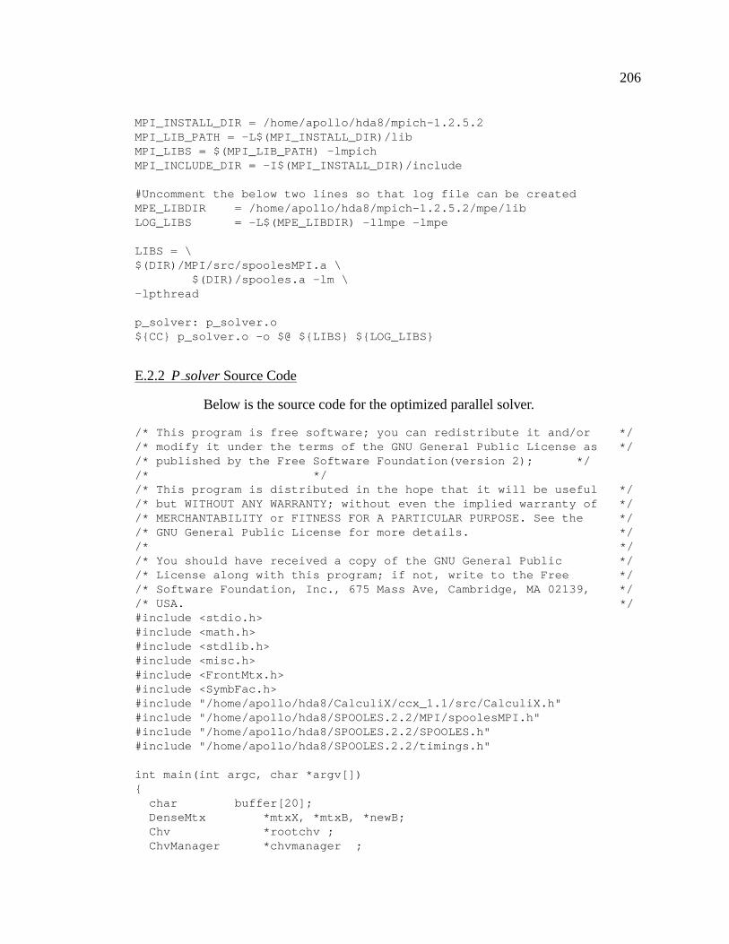
206
MPI_INSTALL_DIR = /home/apollo/hda8/mpich-1.2.5.2MPI_LIB_PATH = -L$(MPI_INSTALL_DIR)/libMPI_LIBS = $(MPI_LIB_PATH) -lmpichMPI_INCLUDE_DIR = -I$(MPI_INSTALL_DIR)/include
#Uncomment the below two lines so that log file can be createdMPE_LIBDIR = /home/apollo/hda8/mpich-1.2.5.2/mpe/libLOG_LIBS = -L$(MPE_LIBDIR) -llmpe -lmpe
LIBS = \$(DIR)/MPI/src/spoolesMPI.a \
$(DIR)/spooles.a -lm \-lpthread
p_solver: p_solver.o${CC} p_solver.o -o $@ ${LIBS} ${LOG_LIBS}
E.2.2 P solver Source Code
Below is the source code for the optimized parallel solver.
/* This program is free software; you can redistribute it and/or *//* modify it under the terms of the GNU General Public License as *//* published by the Free Software Foundation(version 2); *//* *//* This program is distributed in the hope that it will be useful *//* but WITHOUT ANY WARRANTY; without even the implied warranty of *//* MERCHANTABILITY or FITNESS FOR A PARTICULAR PURPOSE. See the *//* GNU General Public License for more details. *//* *//* You should have received a copy of the GNU General Public *//* License along with this program; if not, write to the Free *//* Software Foundation, Inc., 675 Mass Ave, Cambridge, MA 02139, *//* USA. */#include <stdio.h>#include <math.h>#include <stdlib.h>#include <misc.h>#include <FrontMtx.h>#include <SymbFac.h>#include "/home/apollo/hda8/CalculiX/ccx_1.1/src/CalculiX.h"#include "/home/apollo/hda8/SPOOLES.2.2/MPI/spoolesMPI.h"#include "/home/apollo/hda8/SPOOLES.2.2/SPOOLES.h"#include "/home/apollo/hda8/SPOOLES.2.2/timings.h"
int main(int argc, char *argv[]){char buffer[20];DenseMtx *mtxX, *mtxB, *newB;Chv *rootchv ;ChvManager *chvmanager ;
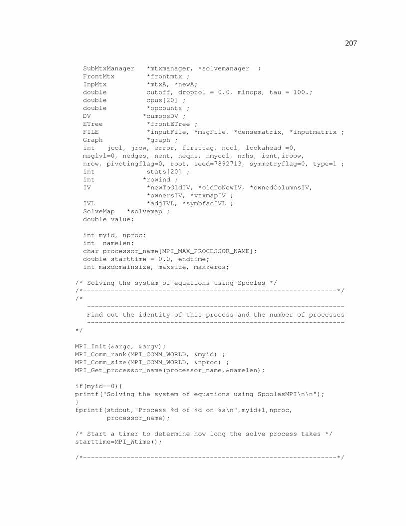
207
SubMtxManager *mtxmanager, *solvemanager ;FrontMtx *frontmtx ;InpMtx *mtxA, *newA;double cutoff, droptol = 0.0, minops, tau = 100.;double cpus[20] ;double *opcounts ;DV *cumopsDV ;ETree *frontETree ;FILE *inputFile, *msgFile, *densematrix, *inputmatrix ;Graph *graph ;int jcol, jrow, error, firsttag, ncol, lookahead =0,msglvl=0, nedges, nent, neqns, nmycol, nrhs, ient,iroow,nrow, pivotingflag=0, root, seed=7892713, symmetryflag=0, type=1 ;int stats[20] ;int *rowind ;IV *newToOldIV, *oldToNewIV, *ownedColumnsIV,
*ownersIV, *vtxmapIV ;IVL *adjIVL, *symbfacIVL ;SolveMap *solvemap ;double value;
int myid, nproc;int namelen;char processor_name[MPI_MAX_PROCESSOR_NAME];double starttime = 0.0, endtime;int maxdomainsize, maxsize, maxzeros;
/* Solving the system of equations using Spooles *//*----------------------------------------------------------------*//*
-----------------------------------------------------------------Find out the identity of this process and the number of processes-----------------------------------------------------------------
*/
MPI_Init(&argc, &argv);MPI_Comm_rank(MPI_COMM_WORLD, &myid) ;MPI_Comm_size(MPI_COMM_WORLD, &nproc) ;MPI_Get_processor_name(processor_name,&namelen);
if(myid==0){printf("Solving the system of equations using SpoolesMPI\n\n");}fprintf(stdout,"Process %d of %d on %s\n",myid+1,nproc,
processor_name);
/* Start a timer to determine how long the solve process takes */starttime=MPI_Wtime();
/*----------------------------------------------------------------*/
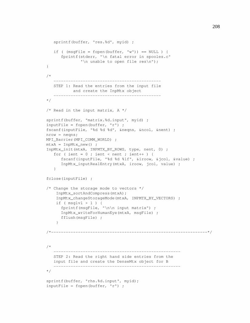
208
sprintf(buffer, "res.%d", myid) ;
if ( (msgFile = fopen(buffer, "w")) == NULL ) {fprintf(stderr, "\n fatal error in spooles.c"
"\n unable to open file res\n");}
/*--------------------------------------------STEP 1: Read the entries from the input file
and create the InpMtx object--------------------------------------------
*/
/* Read in the input matrix, A */
sprintf(buffer, "matrix.%d.input", myid) ;inputFile = fopen(buffer, "r") ;fscanf(inputFile, "%d %d %d", &neqns, &ncol, &nent) ;nrow = neqns;MPI_Barrier(MPI_COMM_WORLD) ;mtxA = InpMtx_new() ;InpMtx_init(mtxA, INPMTX_BY_ROWS, type, nent, 0) ;
for ( ient = 0 ; ient < nent ; ient++ ) {fscanf(inputFile, "%d %d %lf", &iroow, &jcol, &value) ;InpMtx_inputRealEntry(mtxA, iroow, jcol, value) ;
}
fclose(inputFile) ;
/* Change the storage mode to vectors */InpMtx_sortAndCompress(mtxA);InpMtx_changeStorageMode(mtxA, INPMTX_BY_VECTORS) ;if ( msglvl > 1 ) {fprintf(msgFile, "\n\n input matrix") ;InpMtx_writeForHumanEye(mtxA, msgFile) ;fflush(msgFile) ;
}
/*----------------------------------------------------------------*/
/*----------------------------------------------------STEP 2: Read the right hand side entries from theinput file and create the DenseMtx object for B----------------------------------------------------
*/
sprintf(buffer, "rhs.%d.input", myid);inputFile = fopen(buffer, "r") ;
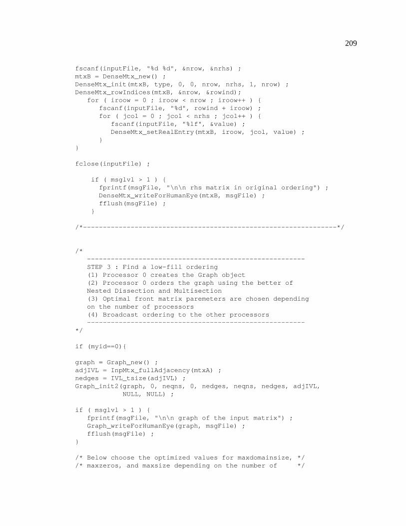
209
fscanf(inputFile, "%d %d", &nrow, &nrhs) ;mtxB = DenseMtx_new() ;DenseMtx_init(mtxB, type, 0, 0, nrow, nrhs, 1, nrow) ;DenseMtx_rowIndices(mtxB, &nrow, &rowind);
for ( iroow = 0 ; iroow < nrow ; iroow++ ) {fscanf(inputFile, "%d", rowind + iroow) ;for ( jcol = 0 ; jcol < nrhs ; jcol++ ) {
fscanf(inputFile, "%lf", &value) ;DenseMtx_setRealEntry(mtxB, iroow, jcol, value) ;
}}
fclose(inputFile) ;
if ( msglvl > 1 ) {fprintf(msgFile, "\n\n rhs matrix in original ordering") ;DenseMtx_writeForHumanEye(mtxB, msgFile) ;fflush(msgFile) ;
}
/*----------------------------------------------------------------*/
/*-------------------------------------------------------STEP 3 : Find a low-fill ordering(1) Processor 0 creates the Graph object(2) Processor 0 orders the graph using the better ofNested Dissection and Multisection(3) Optimal front matrix paremeters are chosen dependingon the number of processors(4) Broadcast ordering to the other processors-------------------------------------------------------
*/
if (myid==0){
graph = Graph_new() ;adjIVL = InpMtx_fullAdjacency(mtxA) ;nedges = IVL_tsize(adjIVL) ;Graph_init2(graph, 0, neqns, 0, nedges, neqns, nedges, adjIVL,
NULL, NULL) ;
if ( msglvl > 1 ) {fprintf(msgFile, "\n\n graph of the input matrix") ;Graph_writeForHumanEye(graph, msgFile) ;fflush(msgFile) ;
}
/* Below choose the optimized values for maxdomainsize, *//* maxzeros, and maxsize depending on the number of */
210
/* processors. */
if (nproc==2){maxdomainsize=700; maxzeros=1000; maxsize=96;}else if (nproc==3){maxdomainsize=900; maxzeros=1000; maxsize=64;}else{maxdomainsize=900; maxzeros=1000; maxsize=80;}
/* Perform an ordering with the better of nested dissection and *//* multi-section. */
frontETree = orderViaBestOfNDandMS(graph,maxdomainsize,maxzeros,maxsize, seed,msglvl,msgFile) ;
Graph_free(graph) ;
}else{}
/* The ordering is now sent to all processors with MPI_Bcast. */
frontETree = ETree_MPI_Bcast(frontETree, root,msglvl, msgFile, MPI_COMM_WORLD) ;
/*----------------------------------------------------------------*//*
-------------------------------------------------------STEP 4: Get the permutations, permute the front tree,
permute the matrix and right hand side.-------------------------------------------------------
*/
/* Very similar to the serial code */oldToNewIV = ETree_oldToNewVtxPerm(frontETree) ;newToOldIV = ETree_newToOldVtxPerm(frontETree) ;ETree_permuteVertices(frontETree, oldToNewIV) ;InpMtx_permute(mtxA, IV_entries(oldToNewIV),
IV_entries(oldToNewIV)) ;InpMtx_mapToUpperTriangle(mtxA) ;InpMtx_changeCoordType(mtxA, INPMTX_BY_CHEVRONS) ;InpMtx_changeStorageMode(mtxA, INPMTX_BY_VECTORS) ;DenseMtx_permuteRows(mtxB, oldToNewIV) ;
211
/*---------------------------------------------------------------*//*
-------------------------------------------STEP 5: Generate the owners map IV object
and the map from vertices to owners-------------------------------------------
*/
/* This is all new from the serial code: *//* Obtains map from fronts to processors. Also a map *//* from vertices to processors is created that enables *//* the matrix A and right hand side B to be distributed*//* as necessary. */cutoff = 1./(2*nproc) ;cumopsDV = DV_new() ;DV_init(cumopsDV, nproc, NULL) ;ownersIV = ETree_ddMap(frontETree,
type, symmetryflag, cumopsDV, cutoff) ;DV_free(cumopsDV) ;vtxmapIV = IV_new() ;IV_init(vtxmapIV, neqns, NULL) ;IVgather(neqns, IV_entries(vtxmapIV),
IV_entries(ownersIV), ETree_vtxToFront(frontETree)) ;if ( msglvl > 1 ) {
fprintf(msgFile, "\n\n map from fronts to owning processes") ;IV_writeForHumanEye(ownersIV, msgFile) ;fprintf(msgFile, "\n\n map from vertices to owning processes") ;IV_writeForHumanEye(vtxmapIV, msgFile) ;fflush(msgFile) ;
}
/*---------------------------------------------------------------*/
/*---------------------------------------------------STEP 6: Redistribute the matrix and right hand side---------------------------------------------------
*/
/* Now the entries of A and B are assembled and distributed */firsttag = 0 ;newA = InpMtx_MPI_split(mtxA, vtxmapIV, stats,
msglvl, msgFile, firsttag, MPI_COMM_WORLD) ;
firsttag++ ;InpMtx_free(mtxA) ;mtxA = newA ;InpMtx_changeStorageMode(mtxA, INPMTX_BY_VECTORS) ;if ( msglvl > 1 ) {
fprintf(msgFile, "\n\n split InpMtx") ;
212
InpMtx_writeForHumanEye(mtxA, msgFile) ;fflush(msgFile) ;
}newB = DenseMtx_MPI_splitByRows(mtxB, vtxmapIV, stats, msglvl,
msgFile, firsttag, MPI_COMM_WORLD) ;DenseMtx_free(mtxB) ;mtxB = newB ;firsttag += nproc ;if ( msglvl > 1 ) {
fprintf(msgFile, "\n\n split DenseMtx B") ;DenseMtx_writeForHumanEye(mtxB, msgFile) ;fflush(msgFile) ;
}
/*---------------------------------------------------------------*/
/*------------------------------------------STEP 7: Compute the symbolic factorization------------------------------------------
*/symbfacIVL = SymbFac_MPI_initFromInpMtx(frontETree, ownersIV, mtxA,
stats, msglvl, msgFile, firsttag, MPI_COMM_WORLD) ;firsttag += frontETree->nfront ;if ( msglvl > 1 ) {
fprintf(msgFile, "\n\n local symbolic factorization") ;IVL_writeForHumanEye(symbfacIVL, msgFile) ;fflush(msgFile) ;
}/*---------------------------------------------------------------*/
/*-----------------------------------STEP 8: initialize the front matrix-----------------------------------
*//* Very similar to the serial code. The arguments, myid and *//* ownersIV tell the front matrix object to initialize only those *//* parts of the factor matrices that it owns */mtxmanager = SubMtxManager_new() ;SubMtxManager_init(mtxmanager, NO_LOCK, 0) ;frontmtx = FrontMtx_new() ;FrontMtx_init(frontmtx, frontETree, symbfacIVL, type, symmetryflag,
FRONTMTX_DENSE_FRONTS, pivotingflag, NO_LOCK, myid,ownersIV, mtxmanager, msglvl, msgFile) ;
/*---------------------------------------------------------------*/
/*---------------------------------STEP 9: Compute the factorization---------------------------------
213
*//* Similar to the serial code */chvmanager = ChvManager_new() ;/* For the serial code, the 0 is replaced by a 1 */ChvManager_init(chvmanager, NO_LOCK, 0) ;rootchv = FrontMtx_MPI_factorInpMtx(frontmtx, mtxA, tau, droptol,
chvmanager, ownersIV, lookahead, &error, cpus,stats, msglvl, msgFile, firsttag,MPI_COMM_WORLD) ;
ChvManager_free(chvmanager) ;firsttag += 3*frontETree->nfront + 2 ;if ( msglvl > 1 ) {
fprintf(msgFile, "\n\n numeric factorization") ;FrontMtx_writeForHumanEye(frontmtx, msgFile) ;fflush(msgFile) ;
}if ( error >= 0 ) {
fprintf(stderr,"\n proc %d : factorization error at front %d", myid, error);
MPI_Finalize() ;exit(-1) ;
}/*---------------------------------------------------------------*//*
------------------------------------------------STEP 10: Post-process the factorization and splitthe factor matrices into submatrices------------------------------------------------
*//* Very similar to the serial code */FrontMtx_MPI_postProcess(frontmtx, ownersIV, stats, msglvl,
msgFile, firsttag, MPI_COMM_WORLD) ;firsttag += 5*nproc ;if ( msglvl > 1 ) {
fprintf(msgFile, "\n\n numeric factorization after post-processing");
FrontMtx_writeForHumanEye(frontmtx, msgFile) ;fflush(msgFile) ;
}/*---------------------------------------------------------------*/
/*-----------------------------------STEP 11: Create the solve map object-----------------------------------
*/solvemap = SolveMap_new() ;SolveMap_ddMap(solvemap, frontmtx->symmetryflag,
FrontMtx_upperBlockIVL(frontmtx),FrontMtx_lowerBlockIVL(frontmtx),nproc, ownersIV, FrontMtx_frontTree(frontmtx),
214
seed, msglvl, msgFile);if ( msglvl > 1 ) {
SolveMap_writeForHumanEye(solvemap, msgFile) ;fflush(msgFile) ;
}/*---------------------------------------------------------------*/
/*----------------------------------------------------STEP 12: Redistribute the submatrices of the factors----------------------------------------------------
*/
/* Now submatrices that a processor owns are local tothat processor */
FrontMtx_MPI_split(frontmtx, solvemap,stats, msglvl, msgFile, firsttag, MPI_COMM_WORLD) ;
if ( msglvl > 1 ) {fprintf(msgFile, "\n\n numeric factorization after split") ;FrontMtx_writeForHumanEye(frontmtx, msgFile) ;fflush(msgFile) ;
}/*---------------------------------------------------------------*/
/*------------------------------------------STEP 13: Create a solution DenseMtx object------------------------------------------
*/ownedColumnsIV = FrontMtx_ownedColumnsIV(frontmtx, myid, ownersIV,
msglvl, msgFile) ;nmycol = IV_size(ownedColumnsIV) ;mtxX = DenseMtx_new() ;if ( nmycol > 0 ) {
DenseMtx_init(mtxX, type, 0, 0, nmycol, nrhs, 1, nmycol) ;DenseMtx_rowIndices(mtxX, &nrow, &rowind) ;IVcopy(nmycol, rowind, IV_entries(ownedColumnsIV)) ;
}/*---------------------------------------------------------------*//*
--------------------------------STEP 14: Solve the linear system--------------------------------
*//* Very similar to the serial code */solvemanager = SubMtxManager_new() ;SubMtxManager_init(solvemanager, NO_LOCK, 0) ;FrontMtx_MPI_solve(frontmtx, mtxX, mtxB, solvemanager, solvemap, cpus,
stats, msglvl, msgFile, firsttag, MPI_COMM_WORLD) ;SubMtxManager_free(solvemanager) ;if ( msglvl > 1 ) {
215
fprintf(msgFile, "\n solution in new ordering") ;DenseMtx_writeForHumanEye(mtxX, msgFile) ;
}/*---------------------------------------------------------------*/
/*--------------------------------------------------------STEP 15: Permute the solution into the original ordering
and assemble the solution onto processor 0--------------------------------------------------------
*/DenseMtx_permuteRows(mtxX, newToOldIV) ;if ( msglvl > 1 ) {
fprintf(msgFile, "\n\n solution in old ordering") ;DenseMtx_writeForHumanEye(mtxX, msgFile) ;fflush(msgFile) ;
}
IV_fill(vtxmapIV, 0) ;firsttag++ ;mtxX = DenseMtx_MPI_splitByRows(mtxX, vtxmapIV, stats, msglvl,
msgFile, firsttag, MPI_COMM_WORLD) ;
/* End the timer */endtime=MPI_Wtime();
/* Determine how long the solve operation took */fprintf(stdout,"Total time for %s: %f\n",processor_name,
endtime-starttime);
/* Now gather the solution the processor 0 */if ( myid == 0) {
printf("%d\n", nrow);sprintf(buffer, "x.result");inputFile=fopen(buffer, "w");
for ( jrow = 0 ; jrow < ncol ; jrow++ ) {fprintf(inputFile, "%1.5e\n", DenseMtx_entries(mtxX)[jrow]);}fclose(inputFile);
}
/*----------------------------------------------------------------*/
/* End the MPI environment */MPI_Finalize() ;
/* Free up memory */InpMtx_free(mtxA) ;DenseMtx_free(mtxB) ;FrontMtx_free(frontmtx) ;DenseMtx_free(mtxX);

216
IV_free(newToOldIV);IV_free(oldToNewIV);ETree_free(frontETree);IVL_free(symbfacIVL);SubMtxManager_free(mtxmanager);
return(0) ;}
REFERENCES
[1] Message Passing Interface Forum. Message passing interface forum home page.Online, October 2003. http://www.mpi-forum.org. 2, 12, 136
[2] Mathematics and Computer Science Division Argonne National Laboratory. Mpich- a portable implementation of mpi. Online, October 2003.http://www-unix.mcs.anl.gov/mpi/mpich/. 2
[3] LAM/MPI Parallel Computing. Lam/mpi parallel computing. Online, April 2005.http://www.lam-mpi.org. 2
[4] Thomas L. Sterling, John Salmon, Donald J. Becker, and Daniel F. Savarese. Howto build a Beowulf: a guide to the implementation and application of PC clusters.MIT Press, Cambridge, MA, 1999. 2
[5] Beowulf.org. Beowulf.org: The beowulf cluster site. Online, October 2003.http://www.beowulf.org. 2
[6] Robert G. Brown. Engineering a beowulf-style compute cluster. Online, January2005.http://www.phy.duke.edu/˜rgb/Beowulf/beowulf_book.php.3, 60
[7] Thomas E. Anderson, David E. Culler, and David A. Patterson. Case for networksof workstations. IEEE Micro, 15(1):54—64, February 1995. 3
[8] Fedora Project. Fedora project, sponsored by red hat. Online, April 2005.http://fedora.redhat.com. 7
[9] The Linux Kernel Archives. The linux kernel archives. Online, May 2005.http://www.kernel.org. 7
[10] Redhat. Red hat enterprise linux documentation. Online, May 2005.http://www.redhat.com/docs/manuals/enterprise/. 8
[11] The Linux Documentation Project. Linux ip masquerade howto. Online, April 2005.http://en.tldp.org/HOWTO/IP-Masquerade-HOWTO/index.html/.8
[12] Netfilter. The netfilger/iptables project. Online, April 2005.http://www.netfilter.org/. 8, 9
217
218
[13] Y. Rekhter, B. Moskowitz, D. Karrenberg, and G. J. de Groot. Address allocationfor private internets. Online, April 2005.ftp://ftp.rfc-editor.org/in-notes/rfc1918.txt. 12
[14] Message Passing Interface Forum. MPI: A Message-Passing Interface Standard.Message Passing Interface Forum, June 1995.http://mpi-forum.org/docs/mpi-11-html/mpi-report.html.12, 13, 144
[15] William Gropp, Ewing Lusk, Nathan Doss, and Anthony Skjellum.High-performance, portable implementation of the mpi standard. ParallelComputing, 22(6):789—829, 1996. 14
[16] William Saphir. A survey of mpi implementations. Technical Report 1, TheNational HPCC Software Exchange, Berkeley, CA, November 1997. 14
[17] The Linux Documentation Project. The linux documentation project. Online, April2005. http://www.tldp.org/. 14, 15
[18] William Gropp and Ewing Lusk. Installation guide to mpich, a portableimplementation of mpi. Online, September 2004.www-unix.mcs.anl.gov/mpi/mpich/docs/install/paper.htm.16
[19] Scalable Computing Laboratory. Netpipe. Online, June 2004.http://www.scl.ameslab.gov/netpipe/. 22
[20] William Gropp, Ewing Lusk, and Thomas Sterling. Beowulf Cluster Computingwith Linux. The MIT Press, Cambridge, MA, second edition, 2003. 22
[21] Myricom. Myricom home page. Online, March 2005.http://www.myri.com/. 23, 168
[22] J. Piernas, A. Flores, and Jose M. Garcia. Analyzing the performance of MPI in acluster of workstations based on fast ethernet. In Proceedings of the 4th EuropeanPVM/MPI Users’ Group Meeting on Recent Advances in Parallel Virtual Machineand Message Passing Interface, volume 1332, pages 17—24, Crackow, Poland,November 1997. Springer. 26, 31
[23] Q. Snell, A. Mikler, and J. Gustafson. Netpipe: A network protocol independentperformace evaluator. Online, June 2004.www.scl.ameslab.gov/netpipe/. 28, 30
[24] University of Tennessee Computer Science Department. Hpl - a portableimplementation of the high-performance linpack benchmark fordistributed-memory computers. Online, January 2004.http://www.netlib.org/benchmark/hpl/. 31, 37, 40, 41, 42, 50
219
[25] R. Clint Whaley and Jack Dongarra. Automatically tuned linear algebra software.Technical Report UT-CS-97-366, University of Tennessee, December 1997. 33
[26] Kazushige Goto. High-performance blas. Online, October 2004.http://www.cs.utexas.edu/users/flame/goto. 34
[27] J. Dongarra, J. Du Croz, S. Hammarling, and I. Duff. A set of level 3 basic linearalgebra subprograms. ACM Transactions on Mathematical Software, 16(1):1—17,March 1990. 50
[28] J. Dongarra, R. Geijn, and D. Walker. Lapack working note 43: A look at scalabledense linear algebra libraries. Technical report, University of Tennessee,Knoxville, TN, 1992. 50
[29] C. Lawson, R. Hanson, D. Kincaid, and F. Krogh. Basic linear algebrasubprograms for fortran usage. ACM Transactions on Mathematical Software,5(3):308—323, September 1979. 50
[30] Guido Dhondt and Klaus Wittig. Calculix: A three-dimensional structural finiteelement program. Online, August 2003. http://www.calculix.de/. 63, 95
[31] Free Software Foundation. The gnu operating system. Online, April 2005.http://www.gnu.org/. 63
[32] Rich Lehoucq, Kristi Maschhoff, Danny Sorensen, and Chao Yang. Arpack -arnoldi package. Online, December 2004.http://www.caam.rice.edu/software/ARPACK. 65
[33] Boeing Phantom Works. Spooles 2.2: Sparse object oriented linear equationssolver. Online, October 2003.http://www.netlib.org/linalg/spooles/spooles.2.2.html.65, 153
[34] Cleve Ashcraft and Roger Grimes. Solving linear systems using spooles 2.2.Online, March 2003.http://www.netlib.org/linalg/spooles/spooles.2.2.html.122, 125, 142
[35] Cleve Ashcraft, Roger Grimes, Daniel Pierce, and David Wah. SPOOLES: AnObject-Oriented Sparse Matrix Library. Boeing Phantom Works, 2002. 122, 125,126
[36] Wikipedia. Object-oriented programming. Online, April 2005.http://en.wikipedia.org/wiki/Object-oriented. 122
220
[37] Cleve Ashcraft, Daniel Pierce, David Wah, and Jason Wu. The Reference Manualfor SPOOLES, Release 2.2: An Object, Oriented Software Library for SolvingSparse Linear Systems of Equations. Boeing Phantom Works, 1999. 122, 129,131, 133, 138, 139, 140, 141, 142
[38] William H. Press, Saul A. Teukolsky, William T. Vetterling, and Brian P. Flannery.Numerical Recipes in Fortran 77 - The Art of Scientific Computing. CambridgeUniversity Press, New York, NY, second edition, 2001. 126
[39] Cleve Ashcraft, Roger Grimes, and J.G. Lewis. Accurate symmetric indefinitelinear equation solvers. Technical report, Boeing Computer Servies, 1995. 126
[40] Cleve Ashcraft. Ordering sparse matrices and transforming front trees. Technicalreport, Boeing Shared Services Group, 1999. 129, 145, 161, 162
[41] Alan George and Joseph W. Liu. Computer Solution of Large Sparse PositiveDefinite Systems. Prentice-Hall, Inc, Englewood Cliffs, NJ, 1981. 130, 145, 147
[42] Timothy Walsh and Leszek Demkowicz. A parallel multifrontal solver forhp-adaptive finite elements. Technical report, The Institute for ComputationalEngineering and Sciences, January 1999. 131
[43] Joseph W. H. Liu. Modification of the minimum-degree algorithm by multipleelimination. ACM Transactions on Mathematical Software, 11(2):141—153, 1985.147, 149, 150
[44] Alan George and Joseph W. H. Liu. The evolution of the minimum degree orderingalgorithm. SIAM Review, 31(1):1—19, 1989. 147
[45] B. Kumar, P. Sadayappan, and C.-H. Huang. On sparse matrix reordering forparallel factorization. In ICS ’94: Proceedings of the 8th international conferenceon Supercomputing, pages 431—438, New York, NY, 1994. ACM Press. 147, 151
[46] Alan George. Nested dissection of a regular finite element mesh. SIAM Journal ofNumerical Analysis, 10:345—363, 1973. 151
[47] Cleve Ashcraft and Joseph W. H. Liu. Robust ordering of sparse matrices usingmultisection. SIAM Journal on Matrix Analysis and Applications, 19(3):816—832,1997. 152
[48] George Karypis. Metis: Family of multilevel partitioning algorithms. Online,October 2004. http://www-users.cs.umn.edu/˜karypis/metis/.152
[49] I. S. Duff, Roger G. Grimes, and John G. Lewis. Sparse matrix test problems.ACM Transactions on Mathematical. Software., 15(1):1—14, 1989. 152

221
[50] Baris Guler, Munira Hussain, Tau Leng, and Victor Mashayekhi. The advantagesof diskless hpc clusters using nas. Online, April 2005.http://www.dell.com. 169

BIOGRAPHICAL SKETCH
Paul C. Johnson was born on October 19, 1980, and grew up in Oppenheim, NY.
He began undergraduate education in the fall of 1998 and received his Bachelor of Sci-
ence in Mechanical Engineering from Manhattan College in May of 2002. Paul continued
his education by pursuing a Master of Science degree in Mechanical Engineering at the
University of Florida. He worked in the Computational Laboratory for Electromagnetics
and Solid Mechanics under the advisement of Dr. Loc Vu-Quoc. His research inter-
ests include adapting and optimizing a parallel system of equations solver to a cluster of
workstations.
222