Embed Size (px)
Citation preview
1
Parallel Computational Chemistry
Alistair Rendell Department of Computer Science
Australian National University([email protected])
International Conference on Computational Science
June 2-4, 2003
Co-located in Melbourne and St Petersburg
• Various workshops (Those in Melbourne)• Computational Chemistry in 21st century
2
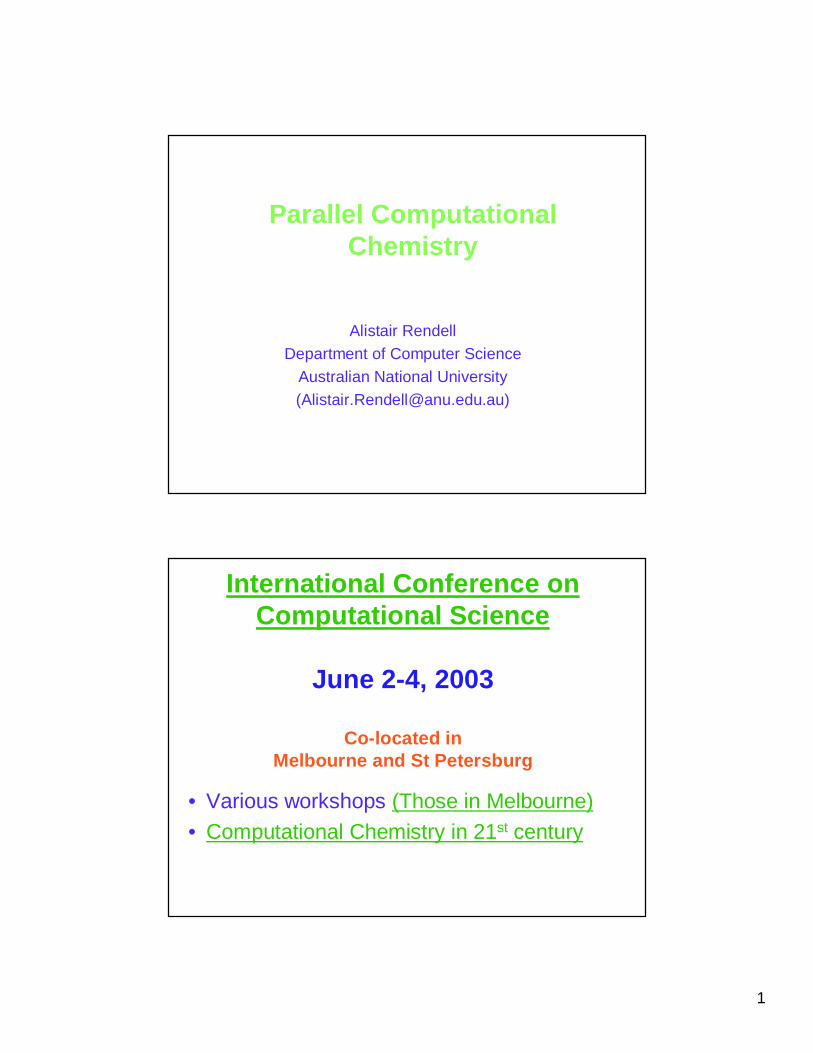
Outline
• Computational Chemistry– All you ever wanted to know in 2 slides!
• Parallel Preface– Understanding your code, computer, compiler
• Parallel Computational Chemistry– OpenMP (Gaussian)– Global Arrays (NWChem)– Charm++ (NAMD)
• Aim– To highlight some things that may be of interest to
people outside the computational chemistry community
Computational Chemistry• The computational study of atoms and
molecules– From physics - chemistry - biology– Includes derivative areas like material science
Critical Issues• Quantum systems
– The interactions of protons, neutrons and electrons are governed by quantum mechanics
• Dynamical systems– Movement is fundamental to chemistry, e.g chemical
reactions, temperature• Size
– A glass of water contains over 1023 water molecules
3
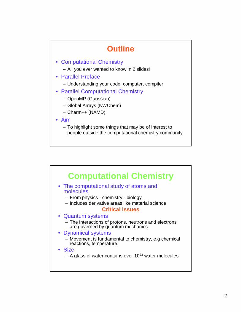
Major Domains• Quantum Chemistry
– Started by people trying to solve the Schrödinger equation for atomic and simple molecular systems, eg H2, LiH
– Now some methods are applicable to hundreds of atoms– Example programs; ADF, GAMESS, Gaussian, QChem etc
• Molecular Dynamics (MD)– Started by people trying to describe the dynamic behavior of a
few hundred atoms interacting via a classical potential– Now tens of thousands of atoms for 10-7 seconds real time– Example programs: Amber, Charmm, Gromos, Tinker etc
• Statistical Mechanics– Take a statistical approach to treating very large system– More home grown codes tailored to particular problem
• Now domains overlap, e.g. quantum MD
Parallel Preface
• Performance benchmarking and tuning– Understanding your code and its performance– Fundamental to both single and parallel processing
• The balance between single processor performance tuning and parallelization– Should you even begin to parallelize a code that runs
at 1% of peak on a single CPU?
4
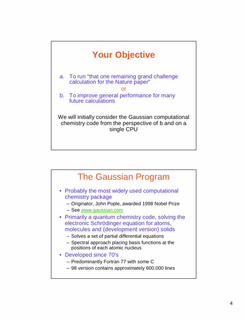
Your Objective
a. To run “that one remaining grand challenge calculation for the Nature paper”
orb. To improve general performance for many
future calculations
We will initially consider the Gaussian computational chemistry code from the perspective of b and on a
single CPU
The Gaussian Program
• Probably the most widely used computational chemistry package– Originator, John Pople, awarded 1998 Nobel Prize– See www.gaussian.com
• Primarily a quantum chemistry code, solving the electronic Schrödinger equation for atoms, molecules and (development version) solids– Solves a set of partial differential equations– Spectral approach placing basis functions at the
positions of each atomic nucleus
• Developed since 70's– Predominantly Fortran 77 with some C– 98 version contains approximately 600,000 lines
5
Issues• Require benchmark calculations that
– Span a range of different widely used functionality– Should complete in "reasonable" time
• Primary input options for Gaussian– Hartree Fock (HF), density functional (BLYP), mixed
(eg B3LYP), perturbation (MP2), coupled cluster etc– Energy, Gradient, Frequency– Gas phase, solvated, solid, electric/magnetic field– Basis set, e.g. 3-21g, cc-pvtz, 6-311++G(3df,3pd)
• Secondary input options– Memory– Input/Output– Sequential/parallel
• Requires knowledge of the application and code
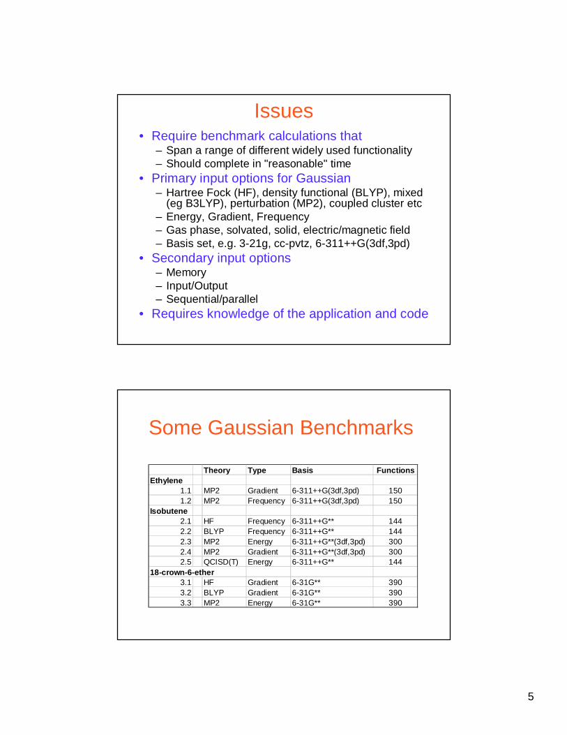
Some Gaussian Benchmarks
Theory Type Basis FunctionsEthylene
1.1 MP2 Gradient 6-311++G(3df,3pd) 1501.2 MP2 Frequency 6-311++G(3df,3pd) 150
Isobutene2.1 HF Frequency 6-311++G** 1442.2 BLYP Frequency 6-311++G** 1442.3 MP2 Energy 6-311++G**(3df,3pd) 3002.4 MP2 Gradient 6-311++G**(3df,3pd) 3002.5 QCISD(T) Energy 6-311++G** 144
18-crown-6-ether3.1 HF Gradient 6-31G** 3903.2 BLYP Gradient 6-31G** 3903.3 MP2 Energy 6-31G** 390
6
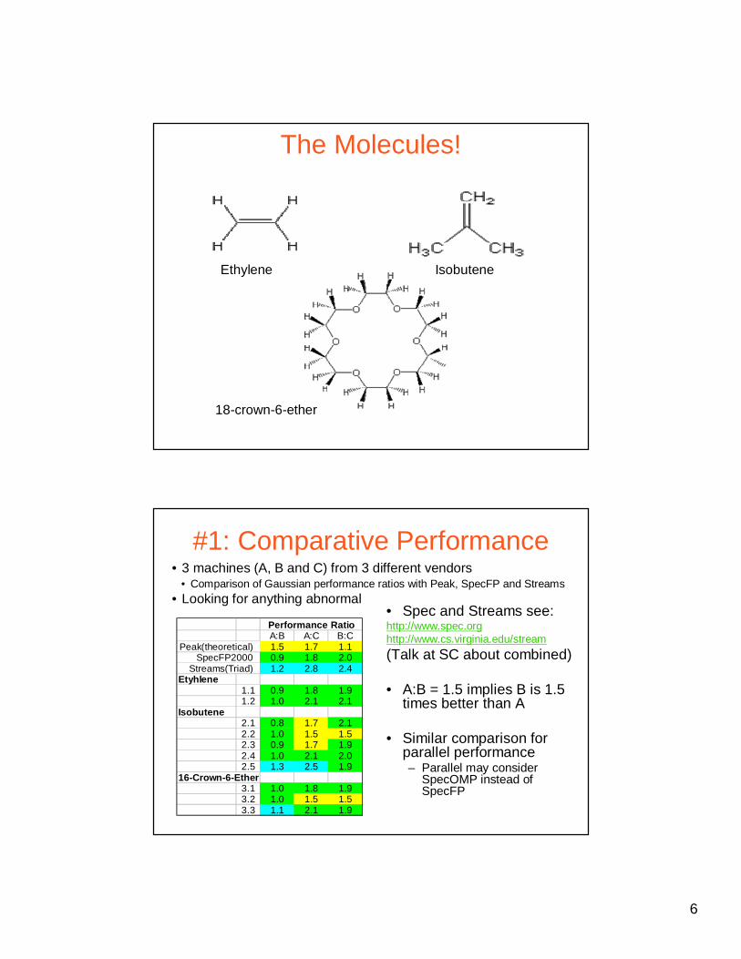
The Molecules!
Ethylene Isobutene
18-crown-6-ether
#1: Comparative Performance
• Spec and Streams see:http://www.spec.orghttp://www.cs.virginia.edu/stream
(Talk at SC about combined)
• A:B = 1.5 implies B is 1.5 times better than A
• Similar comparison for parallel performance– Parallel may consider
SpecOMP instead of SpecFP
• 3 machines (A, B and C) from 3 different vendors• Comparison of Gaussian performance ratios with Peak, SpecFP and Streams
• Looking for anything abnormal
A:B A:C B:C1.5 1.7 1.10.9 1.8 2.01.2 2.8 2.4
Etyhlene1.1 0.9 1.8 1.91.2 1.0 2.1 2.1
Isobutene2.1 0.8 1.7 2.12.2 1.0 1.5 1.52.3 0.9 1.7 1.92.4 1.0 2.1 2.02.5 1.3 2.5 1.9
16-Crown-6-Ether3.1 1.0 1.8 1.93.2 1.0 1.5 1.53.3 1.1 2.1 1.9
Performance Ratio
Peak(theoretical) SpecFP2000
Streams(Triad)
7
#2: Timing and Profiling• Different profilers give different information
• Gprof (all unix systems)– Must recompile with -pg– Resolution of timer can be poor (0.01s)
• Collector/Analyzer (Sun)– Does not require recompilation– Run program under control of collector– Does not provide calling statistics (number of times
routine initiated)
• Profile plus information from calling structure can provide useful information for parallelization of an unknown code
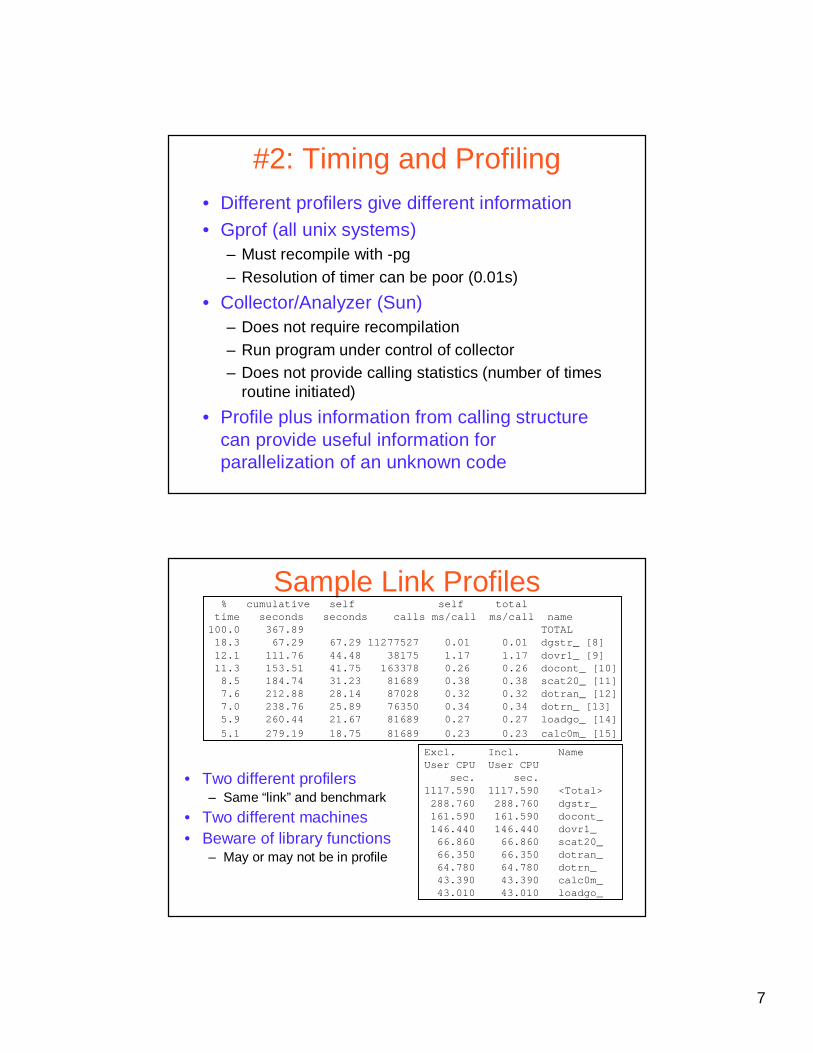
Sample Link Profiles
Excl. Incl. Name User CPU User CPU
sec. sec. 1117.590 1117.590 <Total> 288.760 288.760 dgstr_ 161.590 161.590 docont_ 146.440 146.440 dovr1_ 66.860 66.860 scat20_ 66.350 66.350 dotran_ 64.780 64.780 dotrn_ 43.390 43.390 calc0m_ 43.010 43.010 loadgo_
% cumulative self self total time seconds seconds calls ms/call ms/call name
100.0 367.89 TOTAL18.3 67.29 67.29 11277527 0.01 0.01 dgstr_ [8]12.1 111.76 44.48 38175 1.17 1.17 dovr1_ [9]11.3 153.51 41.75 163378 0.26 0.26 docont_ [10]8.5 184.74 31.23 81689 0.38 0.38 scat20_ [11]7.6 212.88 28.14 87028 0.32 0.32 dotran_ [12]7.0 238.76 25.89 76350 0.34 0.34 dotrn_ [13]5.9 260.44 21.67 81689 0.27 0.27 loadgo_ [14]
5.1 279.19 18.75 81689 0.23 0.23 calc0m_ [15]
• Two different profilers– Same “link” and benchmark
• Two different machines• Beware of library functions
– May or may not be in profile
8
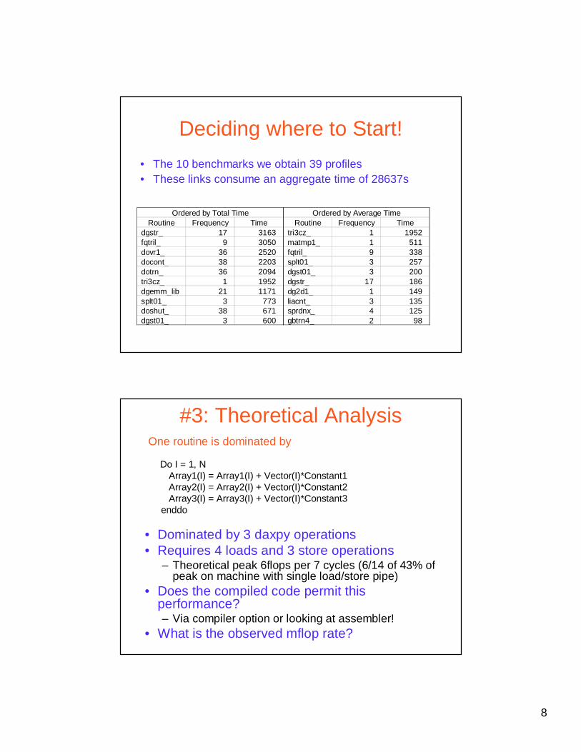
Deciding where to Start!
• The 10 benchmarks we obtain 39 profiles • These links consume an aggregate time of 28637s
Routine Frequency Time Routine Frequency Timedgstr_ 17 3163 tri3cz_ 1 1952fqtril_ 9 3050 matmp1_ 1 511dovr1_ 36 2520 fqtril_ 9 338docont_ 38 2203 splt01_ 3 257dotrn_ 36 2094 dgst01_ 3 200tri3cz_ 1 1952 dgstr_ 17 186dgemm_lib 21 1171 dg2d1_ 1 149splt01_ 3 773 liacnt_ 3 135doshut_ 38 671 sprdnx_ 4 125dgst01_ 3 600 gbtrn4_ 2 98
Ordered by Total Time Ordered by Average Time
#3: Theoretical Analysis
• Dominated by 3 daxpy operations• Requires 4 loads and 3 store operations
– Theoretical peak 6flops per 7 cycles (6/14 of 43% of peak on machine with single load/store pipe)
• Does the compiled code permit this performance?– Via compiler option or looking at assembler!
• What is the observed mflop rate?
Do I = 1, NArray1(I) = Array1(I) + Vector(I)*Constant1Array2(I) = Array2(I) + Vector(I)*Constant2Array3(I) = Array3(I) + Vector(I)*Constant3
enddo
One routine is dominated by
9
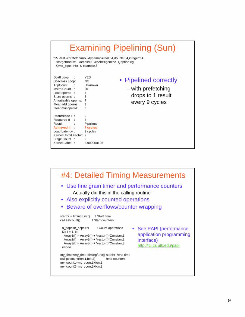
Examining Pipelining (Sun)
• Pipelined correctly– with prefetching
drops to 1 result every 9 cycles
f95 -fast -xprefetch=no -xtypemap=real:64,double:64,integer:64-xtarget=native -xarch=v9 -xcache=generic -Qoption cg -Qms_pipe+info -S example.f
Doall Loop : YESDoacross Loop: NOTripCount : UnknownInstrn Count : 20Load operns : 4Store operns : 3Amortizable operns: 7Float add operns: 3Float mul operns: 3
Recurrence II : 0Resource II : 7Result : PipelinedAchieved II : 7 cyclesLoad Latency : 2 cyclesKernel Unroll Factor: 2Stage Count : 2Kernel Label : .L900000106
#4: Detailed Timing Measurements• Use fine grain timer and performance counters
– Actually did this in the calling routine
• Also explicitly counted operations• Beware of overflows/counter wrapping
starthr = timingfunc() ! Start timecall setcount() ! Start counters
n_flops=n_flops+N ! Count operationsDo I = 1, N
Array1(I) = Array1(I) + Vector(I)*Constant1Array2(I) = Array2(I) + Vector(I)*Constant2Array3(I) = Array3(I) + Vector(I)*Constant3
enddo
my_time=my_time+timingfunc()-starthr !end timecall getcount(fcnt1,fcnt2) !end countersmy_count1=my_count1+fcnt1my_count2=my_count2+fcnt2
• See PAPI (performance application programming interface)http://icl.cs.utk.edu/papi
10
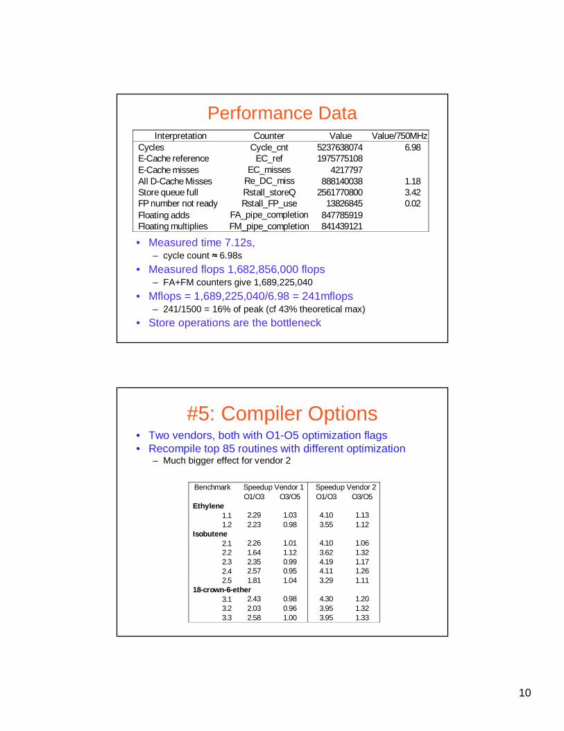
Performance Data
• Measured time 7.12s, – cycle count � 6.98s
• Measured flops 1,682,856,000 flops– FA+FM counters give 1,689,225,040
• Mflops = 1,689,225,040/6.98 = 241mflops– 241/1500 = 16% of peak (cf 43% theoretical max)
• Store operations are the bottleneck
Interpretation Counter Value Value/750MHzCycles Cycle_cnt 5237638074 6.98E-Cache reference EC_ref 1975775108E-Cache misses EC_misses 4217797All D-Cache Misses Re_DC_miss 888140038 1.18Store queue full Rstall_storeQ 2561770800 3.42FP number not ready Rstall_FP_use 13826845 0.02Floating adds FA_pipe_completion 847785919Floating multiplies FM_pipe_completion 841439121
#5: Compiler Options• Two vendors, both with O1-O5 optimization flags• Recompile top 85 routines with different optimization
– Much bigger effect for vendor 2
Benchmark Speedup Vendor 1 Speedup Vendor 2O1/O3 O3/O5 O1/O3 O3/O5
Ethylene1.1 2.29 1.03 4.10 1.131.2 2.23 0.98 3.55 1.12
Isobutene2.1 2.26 1.01 4.10 1.062.2 1.64 1.12 3.62 1.322.3 2.35 0.99 4.19 1.172.4 2.57 0.95 4.11 1.262.5 1.81 1.04 3.29 1.11
18-crown-6-ether3.1 2.43 0.98 4.30 1.203.2 2.03 0.96 3.95 1.323.3 2.58 1.00 3.95 1.33
11
Parallel Computational Chemistry
So you’ve tuned your code and its running at 90% of peak on a single CPU!
…..Then you must using the Earth Simulator!
See: http://www.es.jamstem.go.jpand Gordon Bell awards at SC2002
http://access.ncsa.uiuc.edu/Releases/11.21.02_SC2002_Con.html
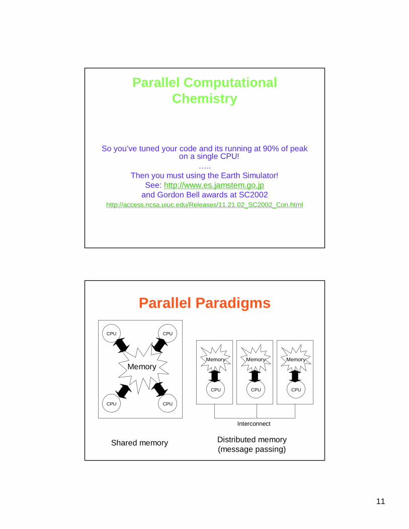
Parallel Paradigms
CPU
Memory
Memory
CPU
CPU CPU
CPU
CPU
Memory
CPU
Memory
Shared memory Distributed memory(message passing)
Interconnect
12
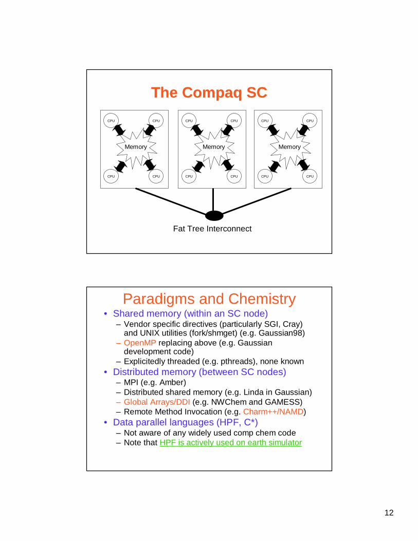
The Compaq SC
Memory
CPU
CPU CPU
CPU
Fat Tree Interconnect
Memory
CPU
CPU CPU
CPU
Memory
CPU
CPU CPU
CPU
Paradigms and Chemistry• Shared memory (within an SC node)
– Vendor specific directives (particularly SGI, Cray) and UNIX utilities (fork/shmget) (e.g. Gaussian98)
– OpenMP replacing above (e.g. Gaussian development code)
– Explicitedly threaded (e.g. pthreads), none known• Distributed memory (between SC nodes)
– MPI (e.g. Amber)– Distributed shared memory (e.g. Linda in Gaussian)– Global Arrays/DDI (e.g. NWChem and GAMESS)– Remote Method Invocation (e.g. Charm++/NAMD)
• Data parallel languages (HPF, C*)– Not aware of any widely used comp chem code– Note that HPF is actively used on earth simulator
13
OpenMP
• Forms the basis for the next release of the Gaussian Package on shared memory architectures
• I have direct interest in this through an ARC Linkage Grant with Gaussian Inc and Sun Microsystems“Programming Paradigms, Tools and Algorithms for the Spectral Solution of the Electronic Schrödinger Equation
on Non-Uniform Memory Parallel Processors”
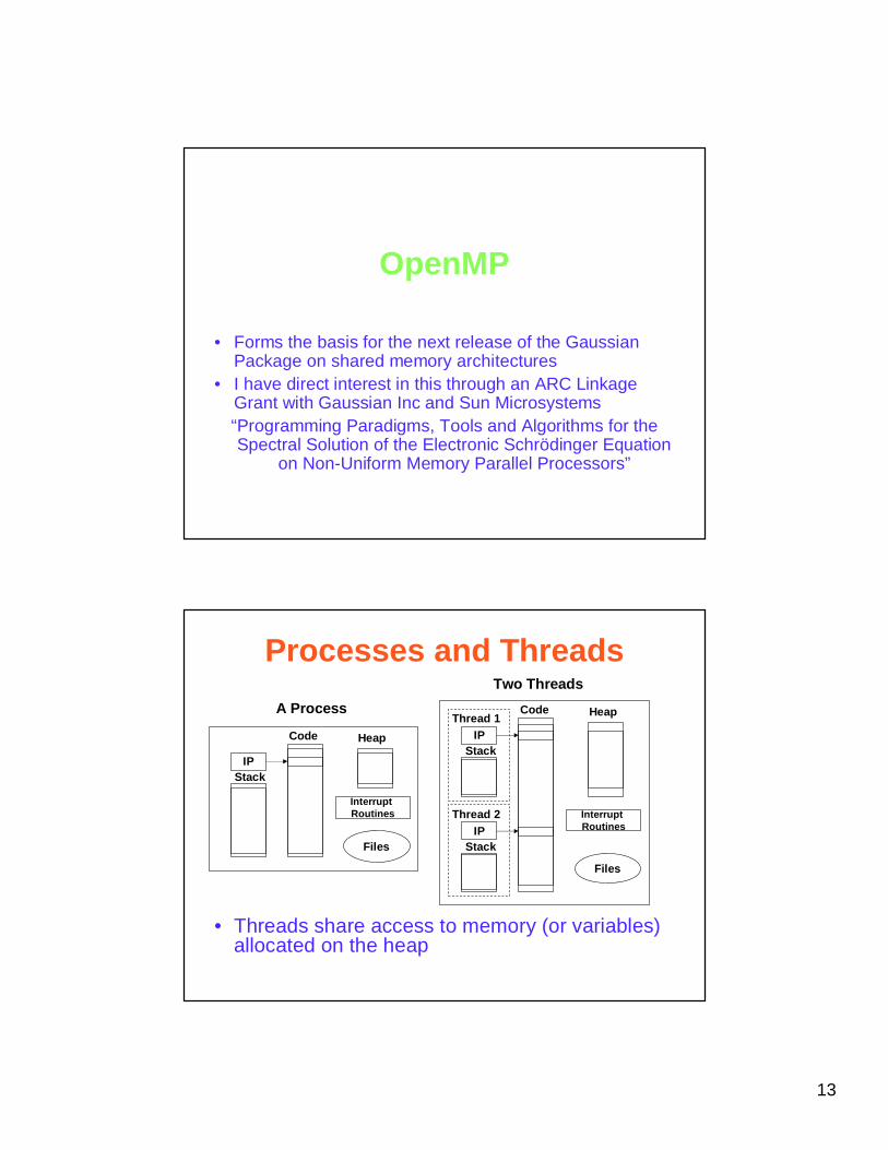
Processes and Threads
IP
Interrupt Routines
Code
Stack
Files
Heap
Interrupt Routines
Code
Files
Heap
IPThread 1
Stack
IPThread 2
Stack
• Threads share access to memory (or variables) allocated on the heap
A Process
Two Threads
14
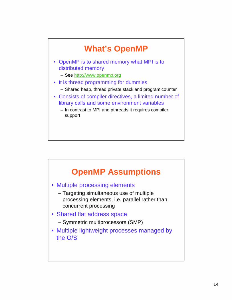
What’s OpenMP• OpenMP is to shared memory what MPI is to
distributed memory– See http://www.openmp.org
• It is thread programming for dummies– Shared heap, thread private stack and program counter
• Consists of compiler directives, a limited number of library calls and some environment variables– In contrast to MPI and pthreads it requires compiler
support
OpenMP Assumptions
• Multiple processing elements– Targeting simultaneous use of multiple
processing elements, i.e. parallel rather than concurrent processing
• Shared flat address space– Symmetric multiprocessors (SMP)
• Multiple lightweight processes managed by the O/S
15
OpenMP History
• 97 – version 1 Fortran standard• 98 – version 1 C and C++ standard• 99 – version 1.1 fixes problems in Fortran version 1• 00 – version 2.0 Fortran
– Support for F90– New directives, COPYPRIVATE– New behavior for old directives, REDUCTION for arrays
• 02 – version 2.0 C and C++• To date there has been a catch up between Fortran and
C versions, in future this will be streamed
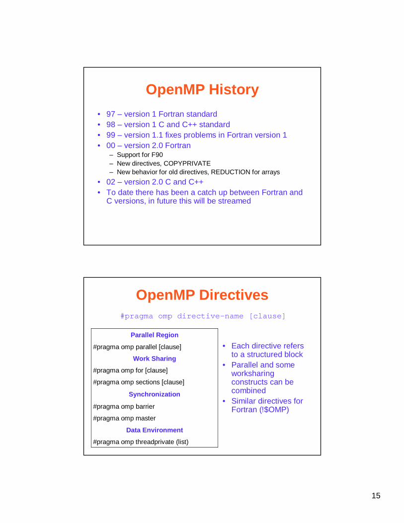
OpenMP Directives
• Each directive refers to a structured block
• Parallel and some worksharingconstructs can be combined
• Similar directives for Fortran (!$OMP)
#pragma omp master
#pragma omp threadprivate (list)
Data Environment
#pragma omp barrier
Synchronization
#pragma omp sections [clause]
#pragma omp for [clause]
Work Sharing
#pragma omp parallel [clause]
Parallel Region
#pragma omp directive-name [clause]
16
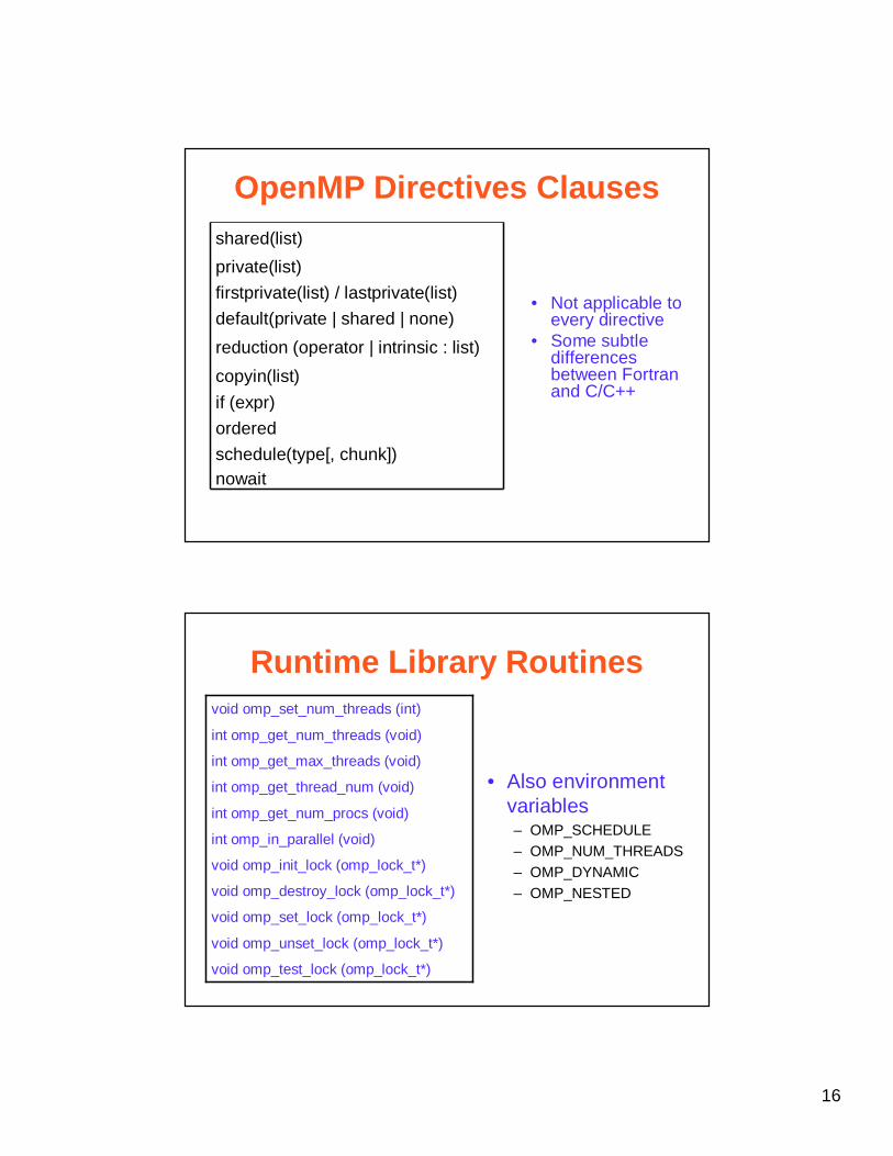
OpenMP Directives Clauses
nowaitschedule(type[, chunk])
ordered
if (expr)
copyin(list)
reduction (operator | intrinsic : list)
default(private | shared | none)
firstprivate(list) / lastprivate(list)
private(list)
shared(list)
• Not applicable to every directive
• Some subtle differences between Fortran and C/C++
Runtime Library Routines
• Also environment variables– OMP_SCHEDULE– OMP_NUM_THREADS– OMP_DYNAMIC– OMP_NESTED
void omp_unset_lock (omp_lock_t*)
void omp_test_lock (omp_lock_t*)
void omp_set_lock (omp_lock_t*)
void omp_destroy_lock (omp_lock_t*)
void omp_init_lock (omp_lock_t*)
int omp_in_parallel (void)
int omp_get_num_procs (void)
int omp_get_thread_num (void)
int omp_get_max_threads (void)
int omp_get_num_threads (void)
void omp_set_num_threads (int)

17
Example: Summing Integers
//SEQUENTIAL CODE#include <stdio.h>#define TOTALSUM 10000int main(){ int i, n, sum;
n=TOTALSUM;sum=0;for (i=0; i< n+1; i++)sum+=i;
printf("Sum of %d integers = %d \n", n, sum);}
=
=10000
0i
iSUM
MPI Code
#include <stdio.h>#include <mpi.h>#define TOTALSUM 10000#define NUMTHREADS 4 // Not determined by MPI code
int main( argc, argv )int argc;char **argv;{int rank, size, i, n, lsum=0, sum;
MPI_Init(&argc, &argv );MPI_Comm_rank( MPI_COMM_WORLD, &rank );MPI_Comm_size( MPI_COMM_WORLD, &size );
if (!rank) n = TOTALSUM;MPI_Bcast(&n, 1, MPI_INT, 0, MPI_COMM_WORLD);
for (i=rank; i< n+1; i+=size)lsum+=i;
MPI_Allreduce(&lsum, &sum, 1, MPI_INT, MPI_SUM, MPI_COMM_WORLD);if (!rank) printf("Sum of %d integers = %d \n", n,sum);
MPI_Barrier(MPI_COMM_WORLD);MPI_Finalize( );return 0;
}
18
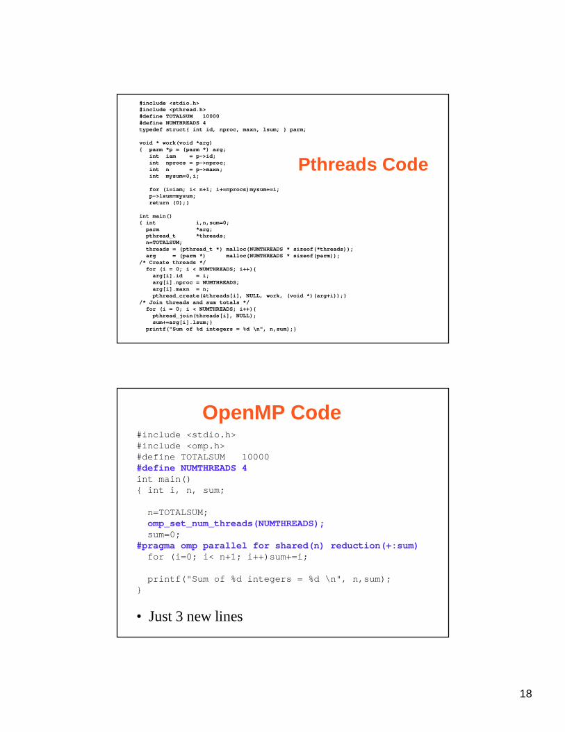
Pthreads Code
#include <stdio.h>#include <pthread.h>#define TOTALSUM 10000#define NUMTHREADS 4typedef struct{ int id, nproc, maxn, lsum; } parm;
void * work(void *arg){ parm *p = (parm *) arg;
int iam = p->id;int nprocs = p->nproc;int n = p->maxn;int mysum=0,i;
for (i=iam; i< n+1; i+=nprocs)mysum+=i;p->lsum=mysum;return (0);}
int main(){ int i,n,sum=0;
parm *arg;pthread_t *threads;n=TOTALSUM;threads = (pthread_t *) malloc(NUMTHREADS * sizeof(*threads));arg = (parm *) malloc(NUMTHREADS * sizeof(parm));
/* Create threads */for (i = 0; i < NUMTHREADS; i++){
arg[i].id = i;arg[i].nproc = NUMTHREADS;arg[i].maxn = n;pthread_create(&threads[i], NULL, work, (void *)(arg+i));}
/* Join threads and sum totals */for (i = 0; i < NUMTHREADS; i++){
pthread_join(threads[i], NULL);sum+=arg[i].lsum;}
printf("Sum of %d integers = %d \n", n,sum);}
OpenMP Code#include <stdio.h>#include <omp.h>#define TOTALSUM 10000#define NUMTHREADS 4int main(){ int i, n, sum;
n=TOTALSUM;omp_set_num_threads(NUMTHREADS);sum=0;
#pragma omp parallel for shared(n) reduction(+:sum)for (i=0; i< n+1; i++)sum+=i;
printf("Sum of %d integers = %d \n", n,sum);}
• Just 3 new lines
19
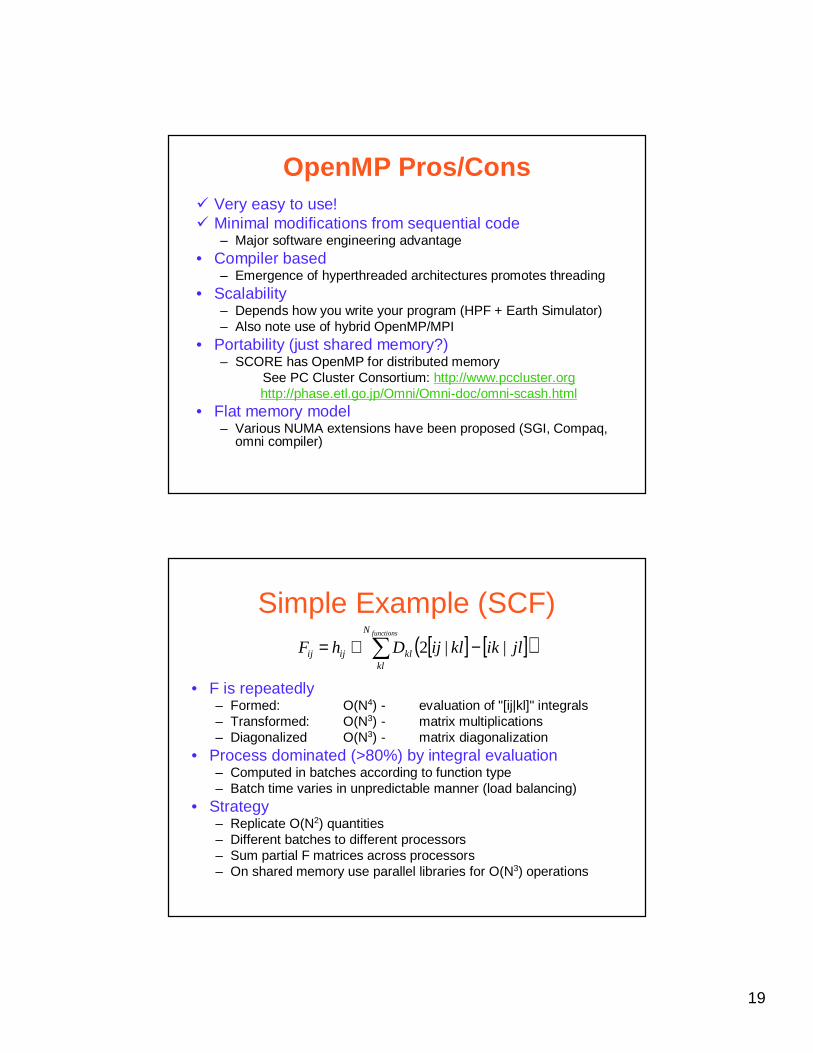
OpenMP Pros/Cons� Very easy to use!� Minimal modifications from sequential code
– Major software engineering advantage • Compiler based
– Emergence of hyperthreaded architectures promotes threading• Scalability
– Depends how you write your program (HPF + Earth Simulator)– Also note use of hybrid OpenMP/MPI
• Portability (just shared memory?)– SCORE has OpenMP for distributed memory
See PC Cluster Consortium: http://www.pccluster.orghttp://phase.etl.go.jp/Omni/Omni-doc/omni-scash.html
• Flat memory model– Various NUMA extensions have been proposed (SGI, Compaq,
omni compiler)
Simple Example (SCF)
• F is repeatedly– Formed: O(N4) - evaluation of "[ij|kl]" integrals– Transformed: O(N3) - matrix multiplications– Diagonalized O(N3) - matrix diagonalization
• Process dominated (>80%) by integral evaluation– Computed in batches according to function type– Batch time varies in unpredictable manner (load balancing)
• Strategy– Replicate O(N2) quantities– Different batches to different processors– Sum partial F matrices across processors– On shared memory use parallel libraries for O(N3) operations
[ ] [ ]( )jlikklijDhFfunctionsN
klklijij ||2 −+=
20
Implementations• Simple UNIX utilities
– Allocate multiple F matrices in a shared memory segment– Assign unique F to each process– Create multiple child processes via fork– Parent process sums partial Fs when children terminate– Some use of parallel libraries
• OpenMP– Generate child processes via PARALLEL DO loop– Assign data structures as PRIVATE or SHARED– Master thread sums partial Fs after parallel loop terminates– Some other loops via directives and use of parallel libraries
• Distributed memory– Linda EVAL function to generate processes– Partial F matrices communicated via Linda IN/OUT operations
O(N3) computation (at least) >> O(N2) communication
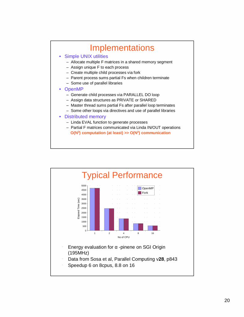
Typical Performance
1 2 4 8 160
500
1000
1500
2000
2500
3000
3500
4000
4500
5000OpenMP
Fork
No of CPU
Ela
pse
d T
ime
(sec
)
" Energy evaluation for α -pinene on SGI Origin (195MHz)
" Data from Sosa et al, Parallel Computing v28, p843" Speedup 6 on 8cpus, 8.8 on 16
21
Global Arrayshttp://www.emsl.pnl.gov:2080/docs/global/ga.html
• Concept that was driven by the computational chemistry group at Pacific Northwest National Laboratory
• Global Arrays or similar are at the heart of the NWChem, Molcas, Molpro and GAMESS-US chemistry codes
• I have developed coupled-cluster and perturbation theory algorithms using Global Arrays
Programming Trade-offsPortability v Efficiency v Ease of Coding
• Shared memory– Greatly simplifies coding but portability and scalability
an issue– Provides little control over data transfer costs
• MPI– Portable– Some applications are too complex to code while
maintaining computational load balance and avoiding redundant computation
• Global Arrays (GA) and the closely related Distributed Data Interface (DDI) attempt to address these issues – For DDI see M.W. Schmidt et al, Comp Phys Com 128,
190 (2000)
22
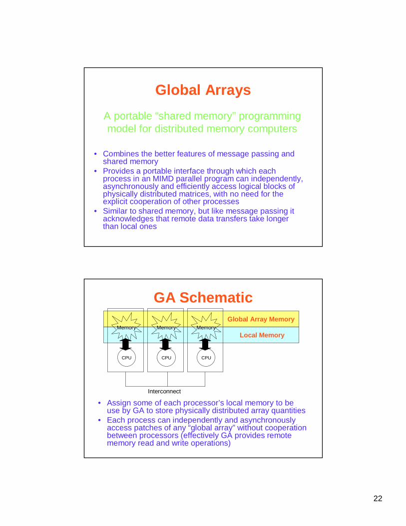
Global Arrays
• Combines the better features of message passing and shared memory
• Provides a portable interface through which each process in an MIMD parallel program can independently, asynchronously and efficiently access logical blocks of physically distributed matrices, with no need for the explicit cooperation of other processes
• Similar to shared memory, but like message passing it acknowledges that remote data transfers take longer than local ones
A portable “shared memory” programming model for distributed memory computers
GA Schematic
CPU
Memory
CPU
Memory
CPU
Memory
Interconnect
Global Array Memory
Local Memory
• Assign some of each processor’s local memory to be use by GA to store physically distributed array quantities
• Each process can independently and asynchronously access patches of any “global array” without cooperation between processors (effectively GA provides remote memory read and write operations)
23
GA Programming Model• MIMD parallelism using multiprocessor approach
– All non-GA data, file descriptors etc are replicated or unique to each process
• Communication achieved by creating and accessing GA matrices augmented (if required) by message passing
• Access to GAs is via get, put, accumulate and get-and-increment operations
• Programmer assumes fast access to parts of a GA that are stored locally, and slower access to the remainder
• Target applications– Task parallel MIMD– Large distributed matrices– Wide variation in task execution time (load balancing)– Large ratio of compute to communicate
GA Functions #1
• Create (and destroy) an array controlling alignment and distribution
• Synchronize all processors• Identify number of processors and my process ID• Fetch, store and accumulate into a patch of an array• Gather/scatter elements of a GA• Atomic read and increment of an array element (shared
counter)• Inquire about location and distribution of an array• Vector and matrix operations on entire GA (eg Array
multiplication)
24
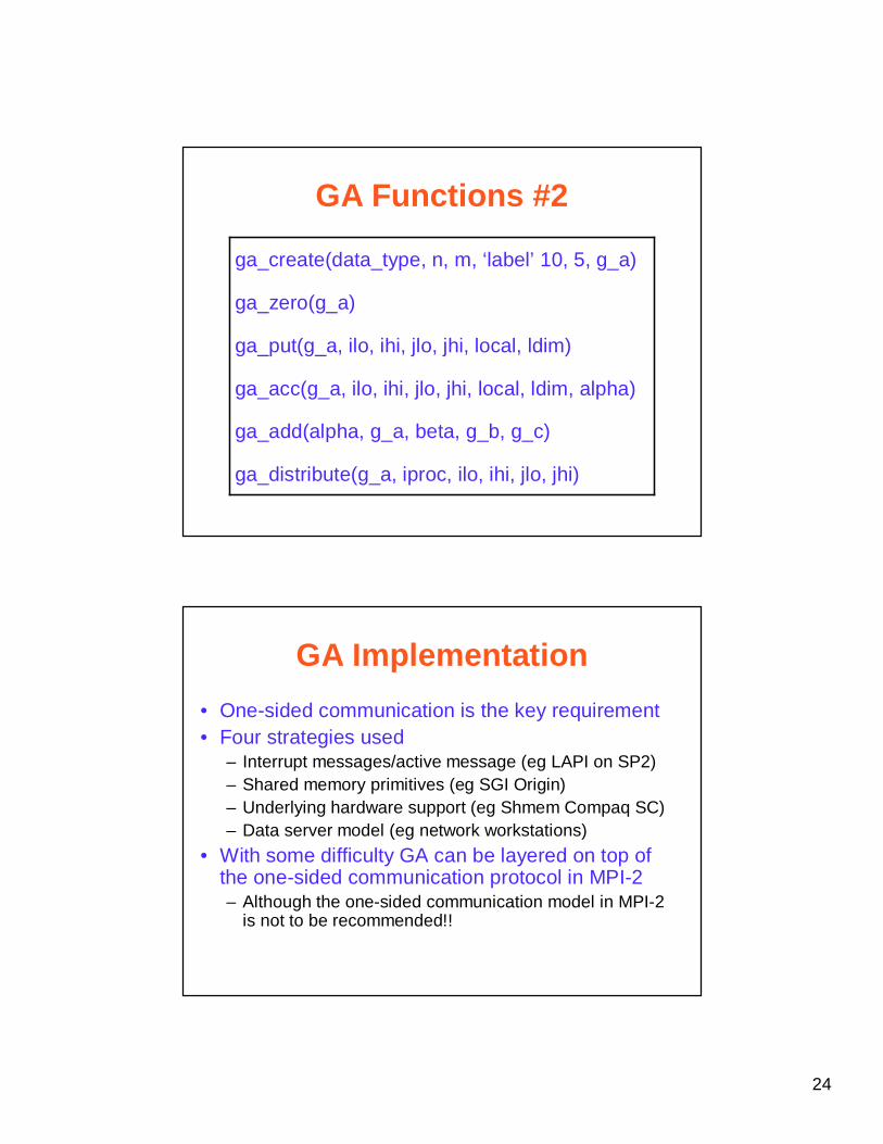
GA Functions #2
ga_distribute(g_a, iproc, ilo, ihi, jlo, jhi)
ga_add(alpha, g_a, beta, g_b, g_c)
ga_acc(g_a, ilo, ihi, jlo, jhi, local, ldim, alpha)
ga_put(g_a, ilo, ihi, jlo, jhi, local, ldim)
ga_zero(g_a)
ga_create(data_type, n, m, ‘label’ 10, 5, g_a)
GA Implementation
• One-sided communication is the key requirement• Four strategies used
– Interrupt messages/active message (eg LAPI on SP2)– Shared memory primitives (eg SGI Origin)– Underlying hardware support (eg Shmem Compaq SC)– Data server model (eg network workstations)
• With some difficulty GA can be layered on top of the one-sided communication protocol in MPI-2– Although the one-sided communication model in MPI-2
is not to be recommended!!
25
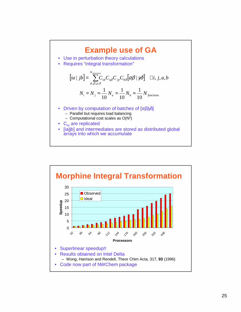
Example use of GA• Use in perturbation theory calculations• Requires “integral transformation”
[ ] [ ]
functionsbaji
bj
N
ai
NNNNN
bajiCCCCjbiafunctions
10
1
10
1
10
1
,,,||,,,
≈=≈=
∀= γδαβδγδγβα
βα
• Driven by computation of batches of [αβ|γδ]– Parallel but requires load balancing– Computational cost scales as O(N5)
• Ciα are replicated• [ia|jb] and intermediates are stored as distributed global
arrays into which we accumulate
Morphine Integral Transformation
0
5
10
15
20
25
30
32 48 64 80 112
144
176
200
256 320 448
Processors
Sp
eed
up
ObservedIdeal
• Superlinear speedup!!• Results obtained on Intel Delta
– Wong, Harrison and Rendell, Theor Chim Acta, 317, 93 (1996)• Code now part of NWChem package
26
NAMD/Charm++
• NAMD is a parallel, object-oriented molecular dynamics program– http://www.ks.uiuc.edu/Research/namd/namd.html
• Employs the prioritized message-driven execution capabilities of the Charm++ parallel runtime system– http://charm.cs.uiuc.edu
• Won a Gordon Bell award at SC02– http://access.ncsa.uiuc.edu/Releases/11.21.02_SC2002_Con.html
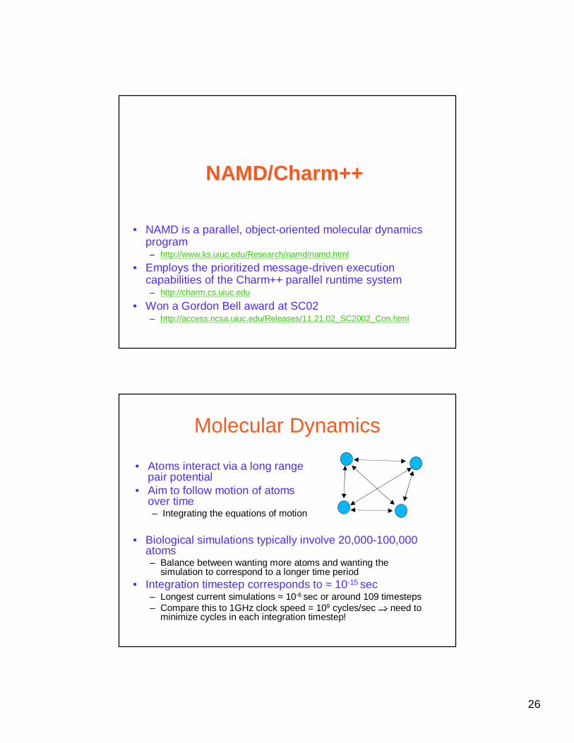
Molecular Dynamics
• Atoms interact via a long range pair potential
• Aim to follow motion of atoms over time – Integrating the equations of motion
• Biological simulations typically involve 20,000-100,000 atoms– Balance between wanting more atoms and wanting the
simulation to correspond to a longer time period• Integration timestep corresponds to ≈ 10-15 sec
– Longest current simulations ≈ 10-6 sec or around 109 timesteps– Compare this to 1GHz clock speed = 109 cycles/sec � need to
minimize cycles in each integration timestep!
27
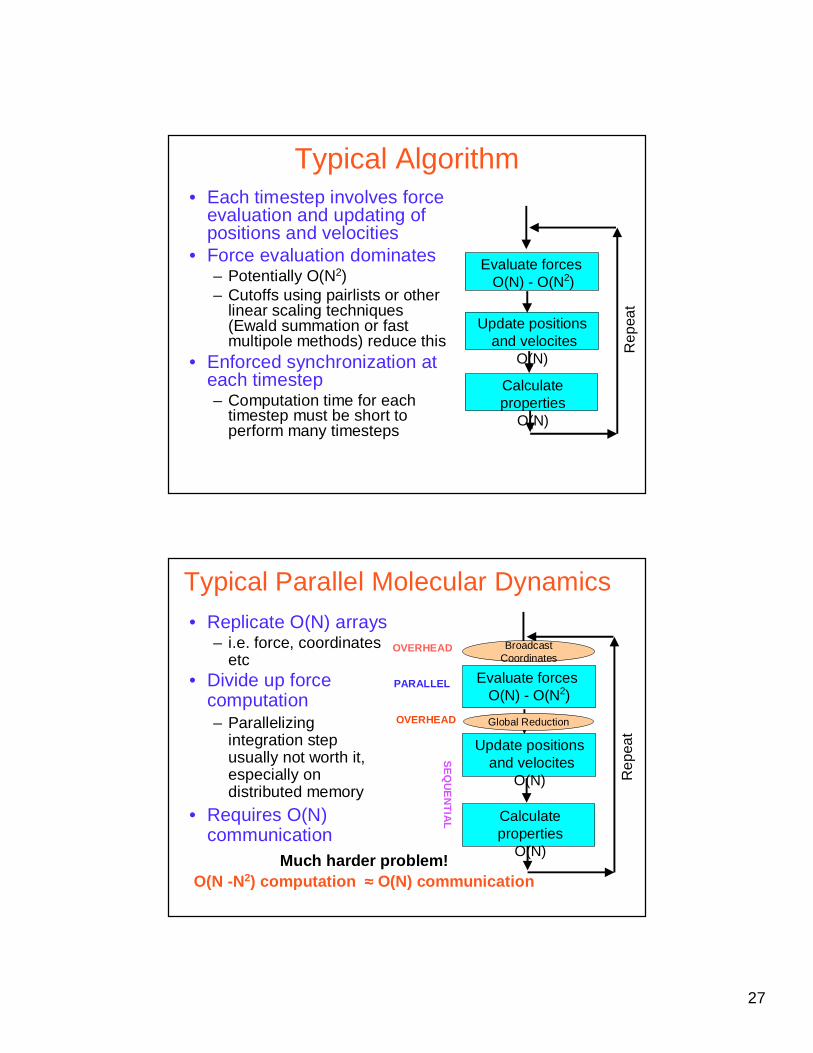
Typical Algorithm• Each timestep involves force
evaluation and updating of positions and velocities
• Force evaluation dominates– Potentially O(N2)– Cutoffs using pairlists or other
linear scaling techniques (Ewald summation or fast multipole methods) reduce this
• Enforced synchronization at each timestep– Computation time for each
timestep must be short to perform many timesteps
Rep
eat
Evaluate forcesO(N) - O(N2)
Update positionsand velocites
O(N)
Calculate properties
O(N)
Typical Parallel Molecular Dynamics
Rep
eat
Evaluate forcesO(N) - O(N2)
Update positionsand velocites
O(N)
Calculate properties
O(N)
• Replicate O(N) arrays– i.e. force, coordinates
etc• Divide up force
computation– Parallelizing
integration step usually not worth it, especially on distributed memory
• Requires O(N) communication
Broadcast Coordinates
Global Reduction
PARALLEL
SE
QU
EN
TIA
L
OVERHEAD
OVERHEAD
Much harder problem!O(N -N2) computation ≈≈≈≈ O(N) communication
28
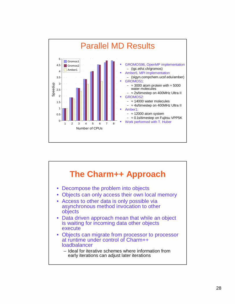
Parallel MD Results
• GROMOS96, OpenMP implementation– (igc.ethz.ch/gromos)
• Amber6, MPI implementation– (sigyn.compchem.ucsf.edu/amber)
• GROMOS1: − ≈ 3000 atom protein with ≈ 5000
water molecules − ≈ 2s/timestep on 400MHz Ultra II
• GROMOS2: − ≈ 14000 water molecules− ≈ 4s/timestep on 400MHz Ultra II
• Amber1: − ≈ 12000 atom system− ≈ 0.1s/timestep on Fujitsu VPP5K
• Work performed with T. Huber1 2 3 4 5 6 7 80
0.5
1
1.5
2
2.5
3
3.5
4
4.5
5Gromos1
Gromos2
Amber1
Number of CPUs
Sp
eedu
p
The Charm++ Approach
• Decompose the problem into objects• Objects can only access their own local memory• Access to other data is only possible via
asynchronous method invocation to other objects
• Data driven approach mean that while an object is waiting for incoming data other objects execute
• Objects can migrate from processor to processor at runtime under control of Charm++ loadbalancer– Ideal for iterative schemes where information from
early iterations can adjust later iterations
29
NAMD• Modern C++ code• Decomposes problem domain into cubes based upon
cutoff radius used in calculation• Objects correspond to force calculations between or
within cubes• Interactions are further partition by type and to increase
the number of objects they may be further split into groups– Aim to have many more objects than processors
• Load balancing performed after running few hundred initial timesteps
• Optimised for to use low level Elan communications on the Pittsburgh Compaq SC
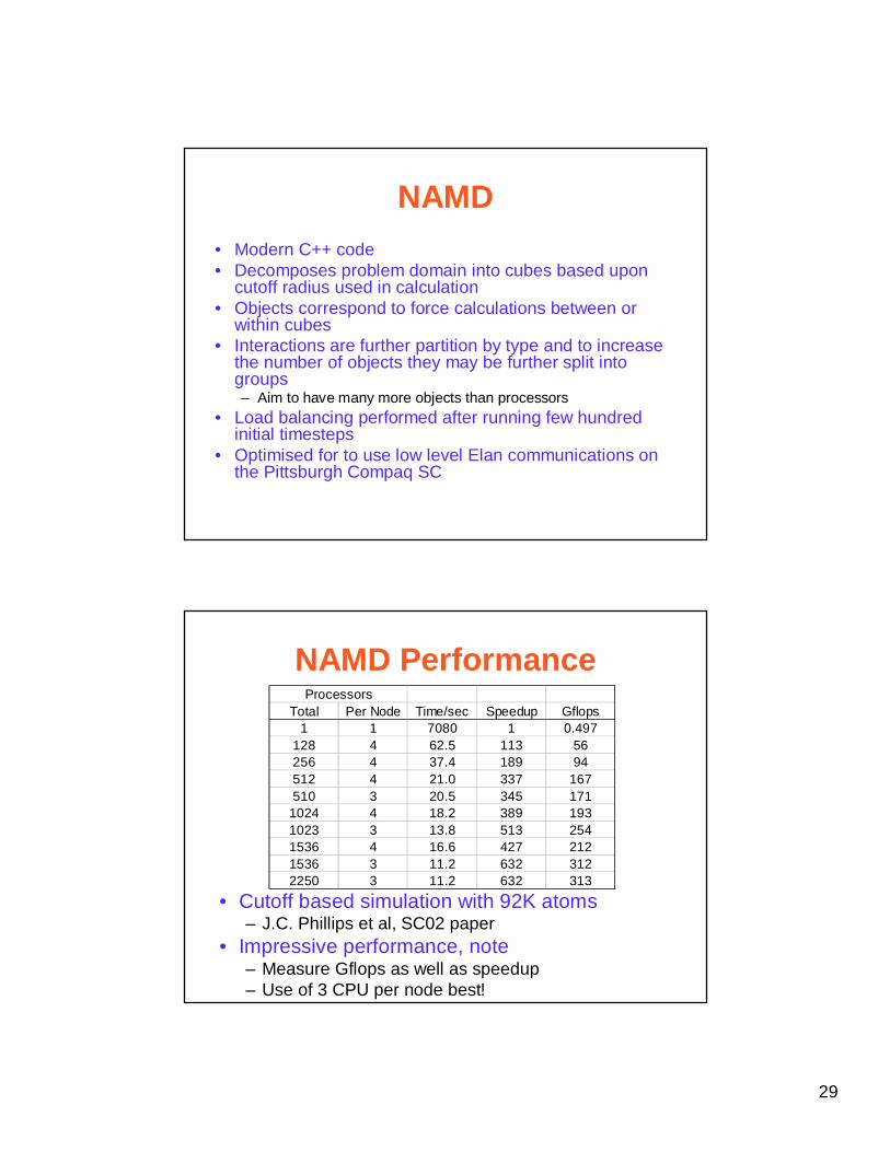
NAMD Performance
• Cutoff based simulation with 92K atoms– J.C. Phillips et al, SC02 paper
• Impressive performance, note– Measure Gflops as well as speedup– Use of 3 CPU per node best!
Total Per Node Time/sec Speedup Gflops1 1 7080 1 0.497
128 4 62.5 113 56256 4 37.4 189 94512 4 21.0 337 167510 3 20.5 345 1711024 4 18.2 389 1931023 3 13.8 513 2541536 4 16.6 427 2121536 3 11.2 632 3122250 3 11.2 632 313
Processors
30
Conclusions
Computational Chemistry Future
• Linear scaling quantum chemical algorithms for large systems!
• Algorithms are based on locality– Bonds, lone pairs etc
• Why now– Increased computer speed enables access of the
crossover point
• The problems– Data placement and retrieval– Load balancing– Computation and communication both O(N)– Software engineering issues
31
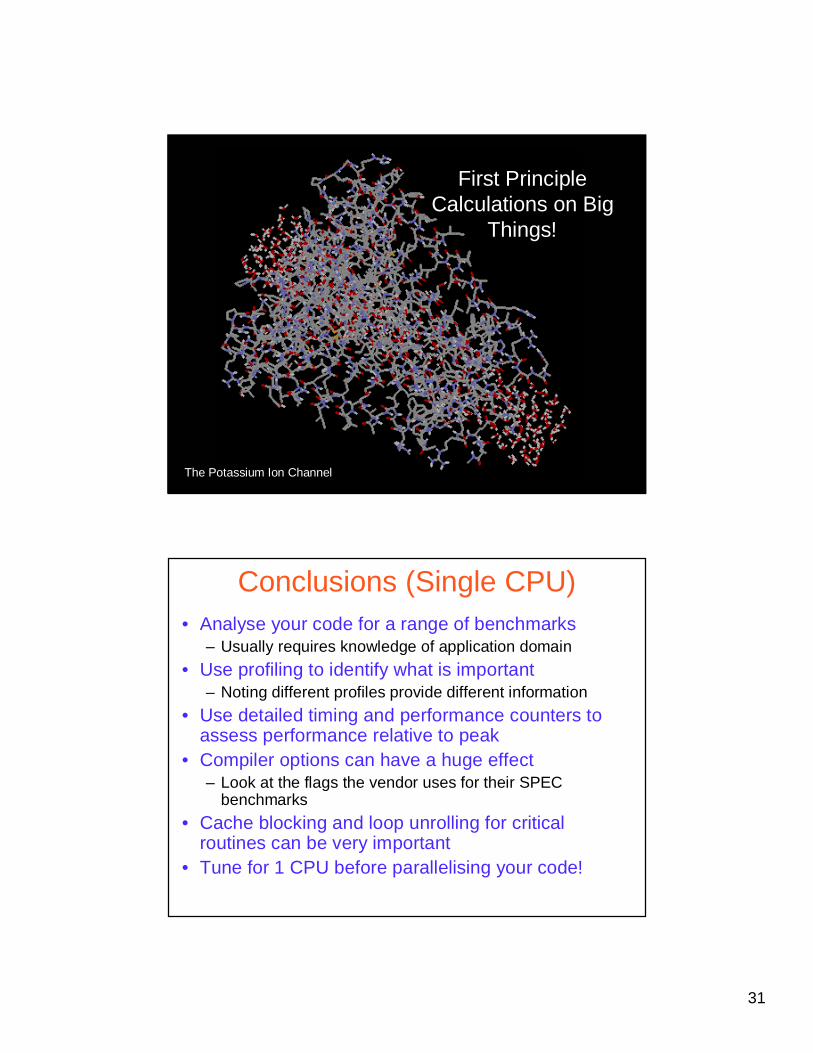
First Principle Calculations on Big
Things!
The Potassium Ion Channel
Conclusions (Single CPU)• Analyse your code for a range of benchmarks
– Usually requires knowledge of application domain
• Use profiling to identify what is important– Noting different profiles provide different information
• Use detailed timing and performance counters to assess performance relative to peak
• Compiler options can have a huge effect– Look at the flags the vendor uses for their SPEC
benchmarks
• Cache blocking and loop unrolling for critical routines can be very important
• Tune for 1 CPU before parallelising your code!
32
Conclusions (Parallel)• Exploiting multiple CPUs is hard
– Must parallelize most of the code– Must minimize overheads– Must load balance your tasks
• Target large problems• Consider which paradigm to use (merits to
both)– Shared or distributed memory– OpenMP/MPI or other
• Code maintenance– Commercial applications need to minimize
difference between multiple version of the same code, especially if code is actively being developed. This is much easier with OpenMP on shared memory, than MPI on distributed memory
Questions
Email [email protected]