University of Nevada, Reno

Parallel Computation, Pattern Recognition,

and Scientific Data Visualization

A professional paper submitted in the partial fulfillment

of the requirements for the degree of Master of Science

with major in Computer Engineering

By

Wenwu CHEN

Dr. Frederick C. Harris, Jr., advisor

August 2003

We recommend that the professional paper

prepared under our supervision by

Wenwu CHEN

entitled

Parallel Computation, Pattern Recognition,

and Scientific Data Visualization

be accepted in partial fulfillment of the

requirements for the degree of

MASTER OF SCIENCE

_________________________________________

Dr. Frederick C. Harris, Jr., Ph. D., Advisor

_________________________________________

Dr. Joseph Cline., Ph. D., Committee Member

_________________________________________

Dr. Carl Looney., Ph. D., Committee Member

_________________________________________

Marsha H. Read, Ph. D., Associate Dean, Graduate School

August 2003

i

Abstract

This professional paper is composed of three projects: the parallel computation in

computational chemistry, the RP-EM-MKL algorithm in pattern recognition, and

scientific data visualization. In the first project, the parallel program on the trajectory

simulation of N2 + NO collision system was implemented using MPI. High efficiency

was obtained and parallel computation could significantly decrease the waiting time for

the simulation. In the second project, the combination of random project (RP),

expectation and maximum (EM) algorithms was applied as an easy and clear approach to

partition the data in multi (MKL) algorithm in the pattern recognition. In the last project,

the GUI project based on QT and OpenGL was designed and implemented to visualize

the Vis5d scientific data.

ii

Acknowledgement

I would like to express my gratitude to all of those who helped me to complete

this professional paper on time. Special thanks are due to my advisor, Professor Harris,

for his help, guidance and support through my academic career in computer science at

UNR, which were vital for this paper. I would like to acknowledge my great appreciation

to Professor J. I. Cline and Dr. George Bebis for their help and guidance on the projects

in the paper. I am also very grateful to Professor Looney for his valuable time and

suggestions and for serving on my committee. Especially, I would like to give my special

thanks to my wife, Yi Wang, for her love, encouragement and support throughout my

education.

iii

Contents

Abstract i

Acknowledgement ii

List of Figures v

1. Introduction 1

2. Parallel Computation in Chemistry 3 2.1 Introduction ……………………………………………………………. 3 2.2 Simulation Principle …………………………………………………… 6 2.3 Parallel Implementation ……………………………………………….. 9 2.4 Results and Discussion ……………………………………………….. 10 2.5 Conclusion ……………...…………………………………………….. 14

2.6 Acknowledgement …………………………………………………….… 14

3. Pattern Recognition with RP-EM-MKL 15 3.1 Introduction ……………………………………………………………. 15 3.2 Algorithms ………………………………………………………….…. 16

3.2.1 PCA algorithm ……………………………………………….….. 16 3.2.2 MKL algorithm ……………………………………………….….. 18 3.3.3 RP-EM-MKL ……………………………………………….…… 19

3.3.Experimental Data Sets ………………………………………………..… 21 3.4 Experimental Results ………………………………………………..… 21

3.4.1 The comparison between PCA and RP ………………………...…. 21 3.4.2 RP-EM-MKL ………………………………………………......… 22

3.5 Conclusions ……………………………………………………….….... 32

4. Scientific Data Visualization 33 4.1 Introduction …………………………………………………………….. 33 4.2 The Structure of Vis5D ……………………..…………………….……. 35 4.3 Design, Implementation and Results ……………………………….....… 37 4.4 Future Work ……………………………………………………………. 45 4.5 Conclusions …………………………………………………………..…. 45

iv

5. Conclusions 46

Bibliography 47

v

List of Figures

Fig. 2.1 The relative computing power required for molecular computations at four levels of theory ……….………………………………………………. … 4 Fig. 2.2 Parallel scaling of the NWChem DFT Module for a number of zeolite fragments on a 512-processor IBM SP…………………………………… 6 Fig. 2.3 The coordinate system for N2 + NO collision system ……………………. 7 Fig. 2.4 The master/slave approach used in the parallel implementation …………. 9 Fig. 2.5 The control flow of master and slaves in the parallel implementation …… 11 Fig. 2.6 The speedup of parallel implementation with up to 36 nodes ……………. 13 Fig. 2.7 The efficiency of parallel implementation ………………………………... 13 Fig. 3.1 The comparison of scoring recognition rate and closet recognition rate between RP and PCA with 90 and 20 individuals ……………………….. 24 Fig. 3.2 The recognition rate dependence on the dimensionality of RP subspace and the number of Gaussian components in the mixture on data set 1 …………. 25 Fig. 3.3 The recognition rate dependence on the size of data set for data set 1 ……... 26 Fig. 3.4 The scalability of recognition rate for PCA and RP-EM-MKL for data set 1 . 27 Fig. 3.5 The recognition rate dependence on and the number of Gaussian components in the mixture on data set 2 ………………………………………………….. 28 Fig. 3.6 The recognition rate dependence on the dimensionality of RP subspace on data set 2 …………………………………………………………………….. 29 Fig. 3.7 The recognition rate dependence on the size of data set for data set 2 ……... 30 Fig. 3.8 The scalability of recognition rate for PCA and RP-EM-MKL for data set 2 .. 31 Fig. 4.1 The screen snap shot for Vis5D project …………………………………….... 33 Fig. 4.2 The control flow of Vis5D project …………………………………………... 36 Fig. 4.3 The loop to handle the user input event in Vis5D …………………………… 36 Fig. 4.4 The diagram of MVC ………………………………………………………... 38 Fig. 4.5 The diagram of the implemented classes for Vis5D data ……………………. 39 Fig. 4.6 The screen snap shots for the visualization of Vis5D data …………………... 39 Fig. 4.7 The diagram of the implemented classes for Topo data ……………………... 41 Fig. 4.8 The screen snap shots for the visualization of Topo data ……………………. 42 Fig. 4.9 The diagram of the implemented classes for flight path ……………………... 43 Fig. 4.10 The screen snap shots to extract the data along the flight path ……………... 44

1

Chapter 1

Introduction It is human knowledge that makes the human being the most distinguished

creature on earth. Man can not only acquire the knowledge for his own experience, but

also obtain the knowledge from the others and inherit the knowledge from the

predecessors, which could speed up the developing of the human knowledge. The human

knowledge is obtained or concluded from various information directly or indirectly. The

revolution in information technology, especially the extensive usage of computer and the

progress of computer science in the 1980s and 1990s, greatly accelerated the acquiring,

developing, sharing and preserving of human knowledge, and pushed the humanity into

information age. Computer science is playing a more and more important role in the

development of human knowledge from the collecting of various raw data and

information (directly or indirectly), analysis of raw data, to the storage and querying of

information and knowledge. Computer science could be found in almost every field

related to information and human knowledge.

The human knowledge system consists of 3 layers: raw data, information and

knowledge. Computer science is involved in each layer of the human knowledge system,

and the computer expands the methods to obtain the information. For example, the

computer can help a researcher build non-natural environments to obtain raw data, to

analysis the data by extracting the information from raw data, and to make the

contribution to human knowledge.

Moreover the computer could also break the space and time obstacles for

knowledge sharing and distribution. There is little restriction in obtaining information due

to the geographical and time obstacles. New techniques can be shared and applied

globally in a short period of time. Man can get related information from hundreds or

thousands of miles away, or several hundred years ago easily with the help of networks

and computers. Human beings are no longer isolated, they can communicate with each

other, exchange and share information easily.

2

The importance of the computer in the development of human knowledge lies in

its powerful computing capacity. With the enormous progress made in hardware and

software, the computer and computer science significantly improve human knowledge. In

the meantime, the improvement in human knowledge requires the more powerful

computers. The information to be dealt with has exponentially exploded. Exchanging and

sharing of information is becoming more and more essential and important. Among many

various solutions, clustered and parallel computing is a mature way to provide the

required computing capability due to its high efficiency and scalability. Recently Grid

computing has attracted more attentions in distributed computing for its large-scale

resource sharing, innovative applications, and high-performance orientation.

Currently human beings are still heavily involved in extracting information from

raw data and extracting knowledge from information. Visualization of raw data and

information is still crucial in the development of human knowledge, and it is also

important for human beings to get information and learn knowledge. Men obtain the most

information and knowledge through visualization. Visualization is an important interface

for interactions between human beings and the computers. Although web services, which

focus on the interaction between/among computers, appear hot recently, they just provide

more concise raw data or information for the man to acquire the knowledge. As long as

human beings are involved, visualization will exist.

This professional paper is on the applications of computer science covering three

categories: parallel computing, pattern recognition, and scientific visualization. It is

organized as the following: Chapter 2 presents the application of parallel computing in

computational chemistry, Chapter 3 presents the use of pattern recognition on face

images, Chapter 4 presents the visualization of the scientific data, such as Vis5D data,

and Chapter 5 give the conclusions.

3

Chapter 2

2.1 Introduction

At the end of his Nobel address in 1966, Dr. Robert S. Mulliken stated that: "In

conclusion, I would like to emphasize my belief that the era of computing chemists, when

hundreds if not thousands of chemists will go to the computing machine instead of the

laboratory, for increasingly many facets of chemical information, is already at hand.

There is only one obstacle, namely, that someone must pay for the computing time."

With the extraordinary progress that has been made in computer science, computing time

is no longer a significant obstacle for computational chemistry. Computational chemistry

is becoming a powerful and indispensable method to solve a variety of problems in

chemistry, both in industrial and in academic chemistry. It was estimated that

computational chemistry accounted for roughly a third of the supercomputer usage

worldwide in 1999.

Computational chemistry is still a relatively new discipline, and there is no

consensus on a precise definition of what computational chemistry actually is. In broad

terms, computational chemistry involves using computers to study chemistry problems,

which complements the areas of theory and experimentation in traditional chemistry

investigation, and helps to direct the experimental chemistry researches in the future.

Computational chemistry covers many wide range aspects of chemistry. It

includes fields from quantum mechanical calculations (such as ab initio and semi-

empirical molecular orbital theory, density functional methods), to classical mechanical

techniques (such as force field, molecular dynamics and Monte Carlo simulations), from

computation of small molecules to molecular modeling of biomolecules (protein, RNA,

DNA), from the synthesis planning, reaction planning to quantitative structure-activity

relationships between drugs and targets, and other techniques applications in

computational chemistry, such as databases, expert systems, artificial intelligence

methods, neural networks.

Computational chemistry provides both qualitative and quantitative insights into

4

many chemical problems. For example, it allows chemists to study chemical phenomena

by running calculations on computers rather than by examining reactions and compounds,

which may be too expensive, too dangerous or too toxic to study experimentally. It can be

used to model not only stable molecules or species, but also short-lived, unstable

intermediates and even non-existing transition states, to verify the experimental results

which is impossible to obtain experimentally through direct observation.

Computational chemistry is based on the use and analysis of mathematical models

on high performance computers, its tasks are normally high computationally and memory

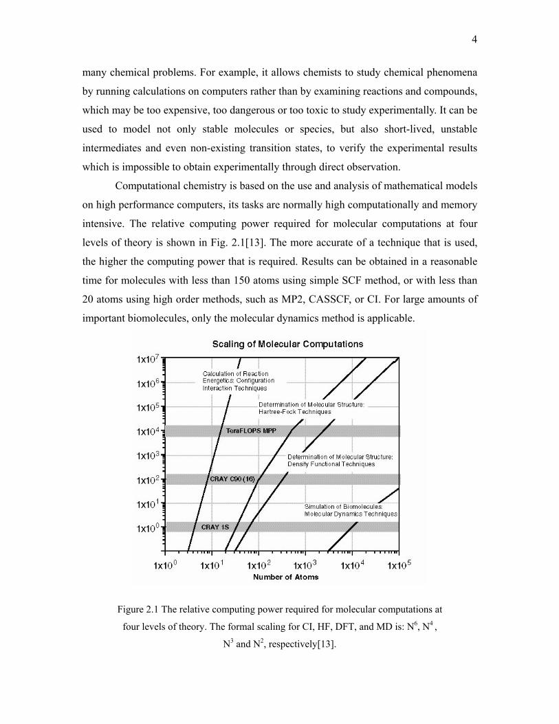
intensive. The relative computing power required for molecular computations at four

levels of theory is shown in Fig. 2.1[13]. The more accurate of a technique that is used,

the higher the computing power that is required. Results can be obtained in a reasonable

time for molecules with less than 150 atoms using simple SCF method, or with less than

20 atoms using high order methods, such as MP2, CASSCF, or CI. For large amounts of

important biomolecules, only the molecular dynamics method is applicable.

Figure 2.1 The relative computing power required for molecular computations at

four levels of theory. The formal scaling for CI, HF, DFT, and MD is: N6, N4 ,

N3 and N2, respectively[13].

5

The required high computation power was only available from the supercomputer,

and large-scale computational chemistry problems were confined to large multi-user

vector and MPP machines a few years ago. However, with the introduction of the cheap

and powerful Intel and AMD CPUs as well as high speed networks, the progress made in

paralleling toolkits, coupled with the growing acceptance of the free Linux operating

system, clusters of low-cost PC machines or workstations can be used to tackle large-

scale chemistry problems. The lower-cost high performance PC clusters and parallel

software offer the exciting possibility to achieve supercomputer performance on a cut-

edge budget to the computational chemists.

Besides the availability of the low-cost high-performance PC machines and

workstations, the basic traits of computation chemistry also make itself ideal for the

parallelizing computation: high intensive computation for each node and much less

communications among nodes. Although communication latency is still a main barrier for

high performance paralleling computation, it is less significant in computational

chemistry due to its above-mentioned traits. Many computational chemistry software

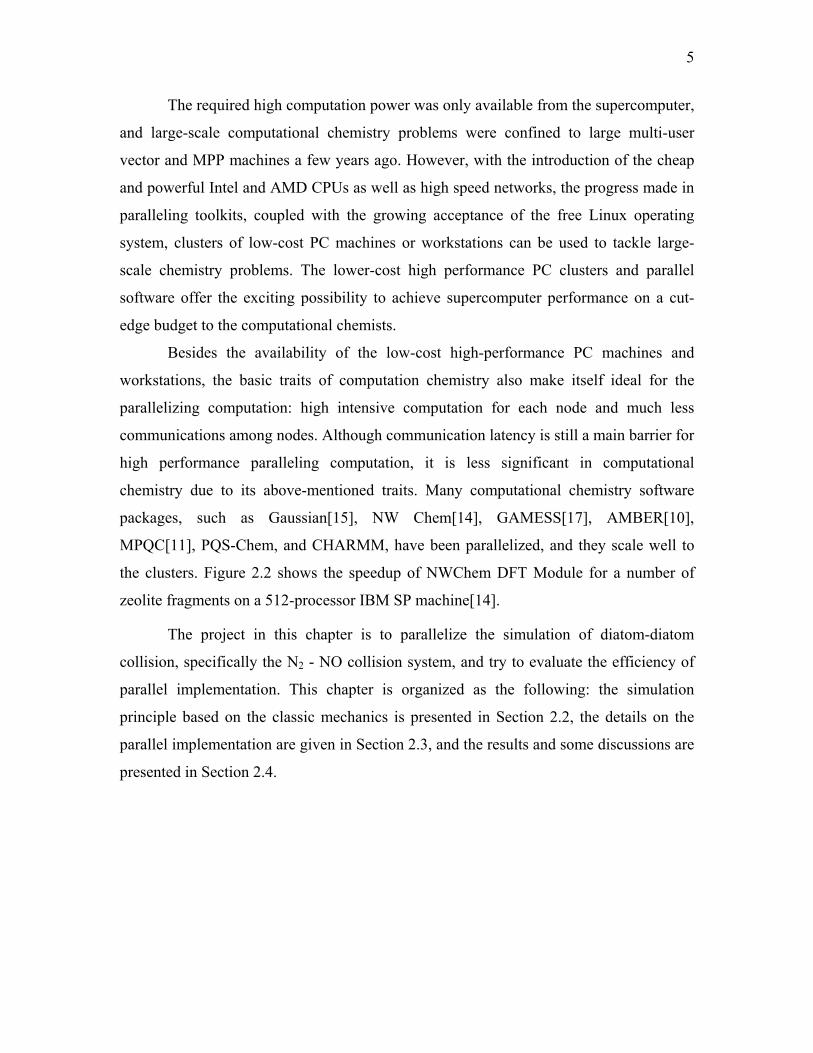
packages, such as Gaussian[15], NW Chem[14], GAMESS[17], AMBER[10],

MPQC[11], PQS-Chem, and CHARMM, have been parallelized, and they scale well to

the clusters. Figure 2.2 shows the speedup of NWChem DFT Module for a number of

zeolite fragments on a 512-processor IBM SP machine[14].

The project in this chapter is to parallelize the simulation of diatom-diatom

collision, specifically the N2 - NO collision system, and try to evaluate the efficiency of

parallel implementation. This chapter is organized as the following: the simulation

principle based on the classic mechanics is presented in Section 2.2, the details on the

parallel implementation are given in Section 2.3, and the results and some discussions are

presented in Section 2.4.

6

Figure 2.2 Parallel scaling of the NWChem DFT Module for a

number of zeolite fragments on a 512-processor IBM SP[14]

2.2 Simulation Principle Computational chemistry is based on mathematical models (which determines the

intra-molecule or inter-molecule interactions), and computer (which provides a medium

to implement the model numerically and generate the simulation results). Basically there

are two kinds of mathematical models in computational chemistry: quantum mechanics

and classical mechanics. Quantum mechanics, such as ab initio, density functional theory,

is more suitable to solve the molecular-level chemistry problems, while classical

mechanics is powerful for the macro-molecular systems. Generally quantum mechanics

model is more complicated to implement, needs more powerful computation resource,

and give more accurate simulations.

Ideally, quantum mechanics should be used to treat the molecular collision, this

could be verified by our previous quantum mechanics treatment on Ar + NO collision

system, in which the quantum mechanics results agree quite well with the experimental

ones[6]. The corresponding classical mechanics simulation approaches the experimental

7

results, but the detailed information is not good enough. However, we have no choice but

to use the classical mechanics simulation for this N2 + NO collision, because:

1. There is no accurate potential energy surface (PES) for this N2 + NO system

available, which is crucial for the quantum mechanics simulation.

2. Too many channels would be involved in this kind of diatomic-diatomic

collision, which may make it impossible to perform the real and reasonable

simulation.

In the classical mechanics simulation, the atom of the molecule or the molecule is

treated as a particle, its motion, describe by its position, is the function of time t. The

position r is described by Newton's second law:

Fi = mi d2ri /dt2

where Fi is the total force for atom i which has mass mi, and its position is described by ri.

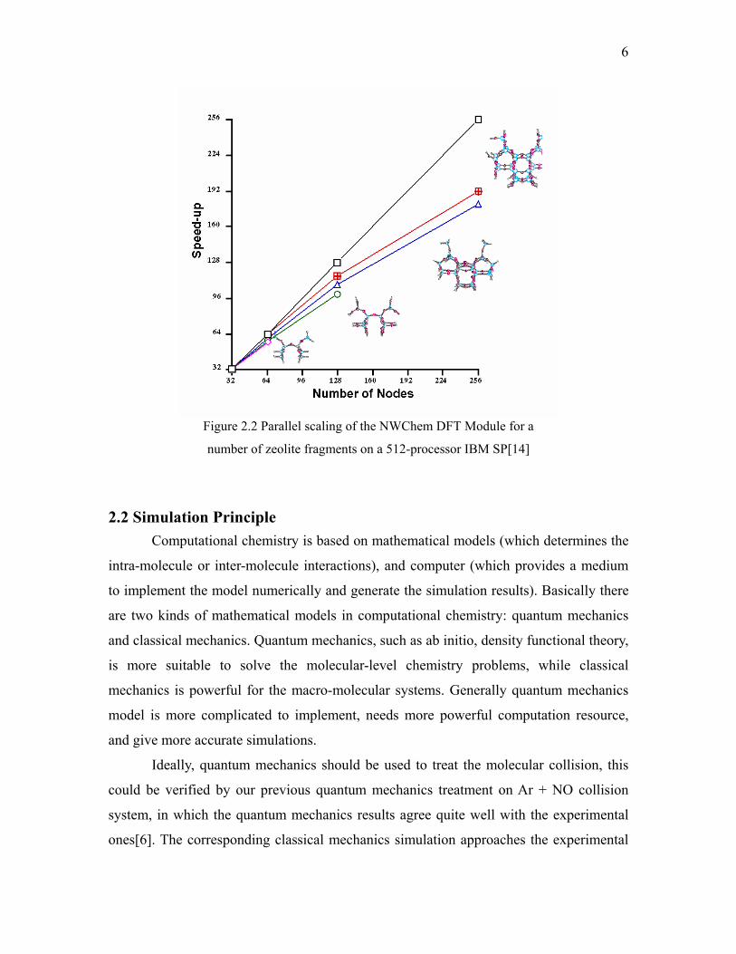
In the specified N2 + NO inelastic collision system, only the translational motion and

rotation of molecules N2 and NO are considered in the project. The coordinate system for

this collision system is shown in Figure 2. 3.

O

2rr

1rrN

N

Rr

Figure 2. 3 The coordinate syste

In this coordinate system, the vec

orientation of molecules N2 and NO, respect

between the centers of mass of these two m

describe by Pr

vector. The motion of the two

equations:

N

m for N2 + NO collision system

tors 1rr and r2

r represent the position and

ively, and Rr

represents the relative position

olecules, and the correspond momentum are

molecules is total by the following coupled

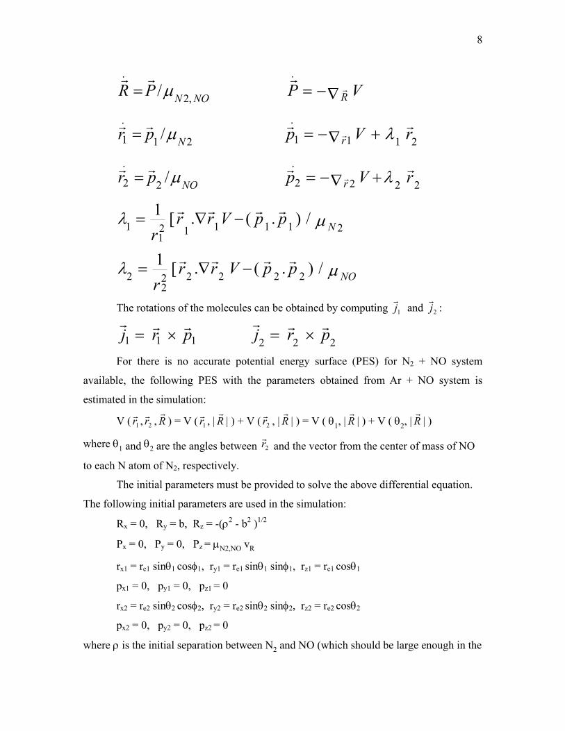
8

NONPR ,2

.

/µrr

= VP R∇−= rr.

21

.

1 / Npr µrr= 211

.

1 rVp rrr

r λ+∇−=

NOpr µ/2

.

2rr

= 222

.

2 rVp rrr

r λ+∇−=

211112

11 /).(.[1

µλ NppVrrr

rrrr−∇=

µλ NOppVrrr

/).(.[122222

22

rrrr−∇=

The rotations of the molecules can be obtained by computing 1jr

and : 2jr

111 prj rrr×= 222 prj rrr

×=

For there is no accurate potential energy surface (PES) for N2 + NO system

available, the following PES with the parameters obtained from Ar + NO system is

estimated in the simulation:

V ( r , r ,1r

2r R

r) = V ( r , |1

r Rr

| ) + V ( 2rr , | R

r| ) = V ( θ1, | R

r| ) + V ( θ2, | R

r| )

where θ1 and θ2 are the angles between r2r

and the vector from the center of mass of NO

to each N atom of N2, respectively.

The initial parameters must be provided to solve the above differential equation.

The following initial parameters are used in the simulation:

Rx = 0, Ry = b, Rz = -(ρ2 - b2 )1/2

Px = 0, Py = 0, Pz = µN2,NO vR

rx1 = re1 sinθ1 cosφ1, ry1 = re1 sinθ1 sinφ1, rz1 = re1 cosθ1

px1 = 0, py1 = 0, pz1 = 0 rx2 = re2 sinθ2 cosφ2, ry2 = re2 sinθ2 sinφ2, rz2 = re2 cosθ2

px2 = 0, py2 = 0, pz2 = 0 where ρ is the initial separation between N2 and NO (which should be large enough in the

9

simulation), vR is the initial relatively velocity (which is determined by the collision

energy), re1 and re2 are equilibrium bond lengths for N2 and NO, respectively, b is the

impact parameter, θ1 , φ1 , θ2 and φ2 are angles. All of these 5 parameters, b, θ1, φ1, θ2 and

φ2, are randomly generated for each trajectory simulation.

2.3 Parallel Implementation The sequential version of the simulation based on above-mentioned classical

mechanics model has been implemented. However the simulation is very time

consuming. In order to obtain the reliable results, thousands of millions of trajectories

should be calculated. Typically it takes approximate 5 days to do 1,000,000 trajectory

simulations in an ordinary Intel PC machine. 10,000,000 trajectories may be needed for

simulation results with good statistics. That many trajectories would need a long time to

be completed in a sequential program simulation. Considering that the calculation for

each trajectory is independent each other, that would be an excellent problem that could

be solved effectively with parallel computation.

The parallel simulation on the trajectory calculation is nearly embarrassingly

parallel computation, in which some initial parameters are distributed among the nodes,

each node performs the trajectory calculation independently, and the final trajectory data

are collected and saved in the file for further processing.

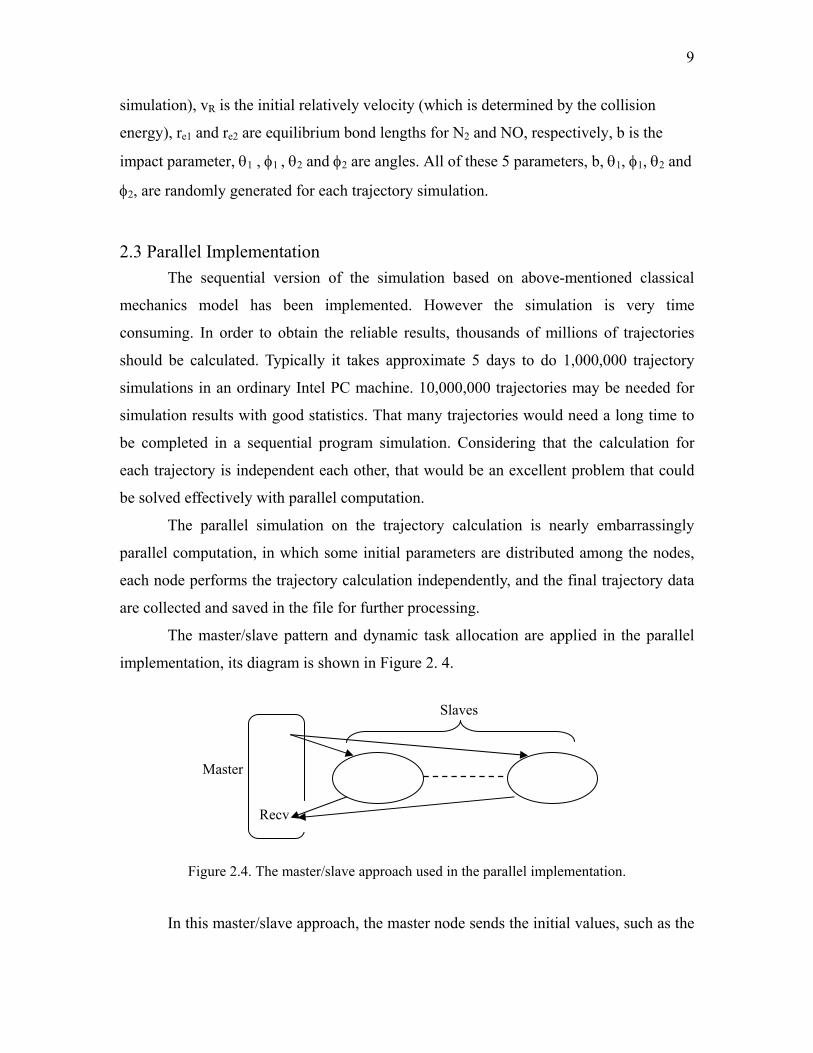
The master/slave pattern and dynamic task allocation are applied in the parallel

implementation, its diagram is shown in Figure 2. 4.

Slaves

Master

Send

Recv

Figure 2.4. The master/slave approach used in the parallel implementation.

In this master/slave approach, the master node sends the initial values, such as the

10

relative velocity vR, the collision parameter ρ, to each slave node to start the trajectory

calculation. Once the slave nodes receive the initial values, they begin the trajectory

simulation independently, send the results, such as the position, velocity for each

trajectory, back to the master, and wait for the commands from the master to decide

whether to continue the calculation or to exit. When the master receives the simulation

result from a slave, it saves the data, and determines whether there are more trajectories

needing to be calculated. If all the trajectories have been calculated, the master sends a

stop message to the slave nodes, otherwise it sends the corresponding initial values to the

slave node to continue the calculation. The master continues this iteration, until it sends

stop message to all the slave nodes. The control flowchart for master and slaves is shown

in Figure 2.5.

2.4 Results and Discussion The parallel version program was implemented using the FORTRAN language

with MPI. The MPI environment we used is the LAM/MPI implementation on an SGI

workstation cluster at the Engineering Computing Center (ECC).This workstation cluster

is composed of up to 40 SGI O2 machines and the nodes are connected via a standard

100 Base Ethernet network.

The main goal of the project is the simulation. In parallel it takes about 5.5 days

for the calculation of 10,000,000 trajectories with 20 nodes, and the final data is about

1.5GB. Several experiments were also done to indicate the powerfulness and efficiency

of the parallel computing for this project, where the calculated trajectory number is fixed

at 1,00,000 to decrease the experimental time. The experiments also indicate the parallel

program has good scalability when changing the number of trajectories computed, which

is the expectation for embarrassingly parallel computations and nearly embarrassingly

parallel computations.

11

traje tion

No

Yes

Exit

Message? Stop

Send results to the master

Receive Command Message from Master

Perform the ctory calcula

Receive initial data from Master

Initialize

Master Slaves

No

No

Yes

Yes

Save data in file

Finish Calculation?

Save data in memory/file

Send Stop Message to Slave

Receive data from Slave

Send initial data to Slave

Initialize

Receive data from

Send Stop to All Slaves?

Exit

Figure 2.5 The control flow of master and slaves in the parallel implementation.

12

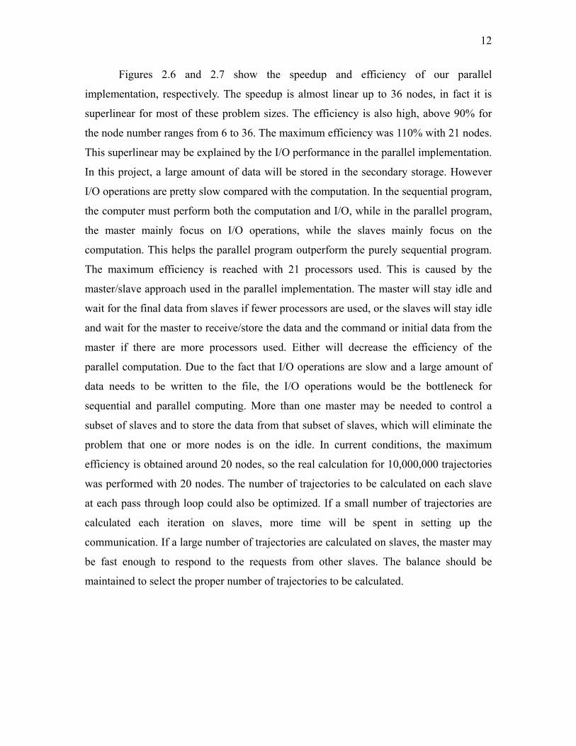
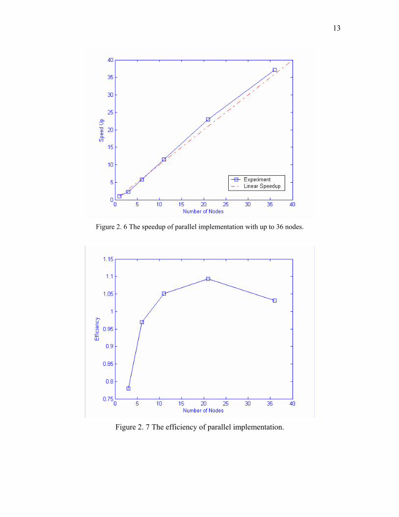
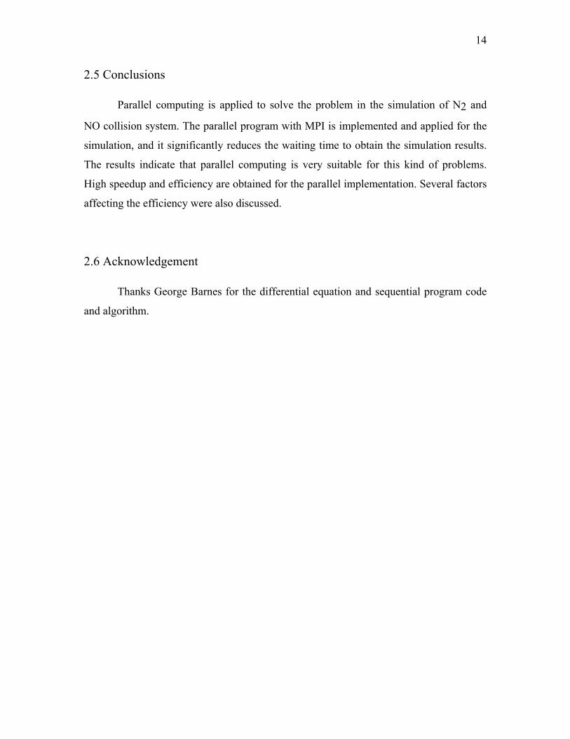
Figures 2.6 and 2.7 show the speedup and efficiency of our parallel

implementation, respectively. The speedup is almost linear up to 36 nodes, in fact it is

superlinear for most of these problem sizes. The efficiency is also high, above 90% for

the node number ranges from 6 to 36. The maximum efficiency was 110% with 21 nodes.

This superlinear may be explained by the I/O performance in the parallel implementation.

In this project, a large amount of data will be stored in the secondary storage. However

I/O operations are pretty slow compared with the computation. In the sequential program,

the computer must perform both the computation and I/O, while in the parallel program,

the master mainly focus on I/O operations, while the slaves mainly focus on the

computation. This helps the parallel program outperform the purely sequential program.

The maximum efficiency is reached with 21 processors used. This is caused by the

master/slave approach used in the parallel implementation. The master will stay idle and

wait for the final data from slaves if fewer processors are used, or the slaves will stay idle

and wait for the master to receive/store the data and the command or initial data from the

master if there are more processors used. Either will decrease the efficiency of the

parallel computation. Due to the fact that I/O operations are slow and a large amount of

data needs to be written to the file, the I/O operations would be the bottleneck for

sequential and parallel computing. More than one master may be needed to control a

subset of slaves and to store the data from that subset of slaves, which will eliminate the

problem that one or more nodes is on the idle. In current conditions, the maximum

efficiency is obtained around 20 nodes, so the real calculation for 10,000,000 trajectories

was performed with 20 nodes. The number of trajectories to be calculated on each slave

at each pass through loop could also be optimized. If a small number of trajectories are

calculated each iteration on slaves, more time will be spent in setting up the

communication. If a large number of trajectories are calculated on slaves, the master may

be fast enough to respond to the requests from other slaves. The balance should be

maintained to select the proper number of trajectories to be calculated.

13

Figure 2. 6 The speedup of parallel implementation with up to 36 nodes.

Figure 2. 7 The efficiency of parallel implementation.

14

2.5 Conclusions

Parallel computing is applied to solve the problem in the simulation of N2 and

NO collision system. The parallel program with MPI is implemented and applied for the

simulation, and it significantly reduces the waiting time to obtain the simulation results.

The results indicate that parallel computing is very suitable for this kind of problems.

High speedup and efficiency are obtained for the parallel implementation. Several factors

affecting the efficiency were also discussed.

2.6 Acknowledgement

Thanks George Barnes for the differential equation and sequential program code

and algorithm.

15

Chapter 3

3.1 Introduction Pattern recognition and pattern reconstruction are two classical problems in

computer vision, and Principal Component Analysis (PCA)[9] (which is usually referred

to as the Karhunen-Loveve transform, or simply KL[5]) is one of the powerful and

widely used technique in pattern reconstruction and pattern recognition. Although PCA

is optimized only for pattern reconstruction in the cases that only a small number of

principal components is sufficient to account for the most structures of the patterns, and it

is a well-known fact that the feature combinations found by PCA could model the

variance of the data set pretty well, but they may not be the same features that separate

the classes, i.e. the PCA components that model the largest contributions to the data set

variance may work poorly for pattern recognition. Extensive experimental and theoretical

studies demonstrate that PCA also perform well for the pattern recognition, and that it

could provide an optimal selection of feature subsets in many cases.

Unfortunately, several intrinsic drawbacks of PCA limit its application in many

practical fields. Theoretically, PCA is one of the linear mapping techniques. It is well

suited to a data set that could be described with one hyper-ellipsoid, i.e. the data set of

one Gaussian distribution. However the practical data set may be approximated more

accurately with multiple Gaussian distributions, which cannot be handled correctly by the

traditional PCA. The natural solution to this problem is to apply PCA to each Gaussian

distribution, which is also the main idea in the MKL algorithm[1]. The main point for

MKL algorithm is how to partition the data into several Gaussian distributions. Two

partition methods have been proposed to partition the data, however, they are

complicated and very time-consuming.

PCA is also quite expensive to perform for the high dimensional data sets. PCA

is actually an orthogonal transform of the coordinate system in which the data set is

described by making use of the eigenvectors of the covariance matrix of the centralized

data. In order to do that, the eigenvalue equation of the covariance matrix needs to be

16

solved, whose running time is O(n3) for n-dimensional data.

One possible solution to the above-mentioned problems is to use the combination

of random projection (RP)[2, 3] and expectation maximization (EM) algorithm[7, 8]. EM

is a standard and effective algorithm to tune the parameters of the Gaussian mixture, but

it can be only applied for the low-dimensionality data set due to the runtime, and

sometimes it encounters the singularity of the covariance problem. These two main

drawbacks of EM algorithm can be solved by applying preprocessing for the data with

random projection technique. As a newly emerged technique for dimensionality

reduction, random projection is simple, easy to implement, but still powerful and accurate

enough. Its two basic theoretical results make it ideal to combine with EM algorithm. The

first is that data from a mixture of k Gaussians can be projected into just O(log k)

dimensions while still retaining the approximate level of separation between the clusters.

The projections dimension is independent of the number of data and of their original

dimension. This property of random projection is very promising for the cases with larger

number of data and with higher dimensionality. The second is that the random projection

will make the clusters more spherical even when the original ones are highly eccentric.

This may be beneficial for EM because it will decrease the possibility of the singularity

of the intermediate covariance matrices.

In this chapter, we propose the application of the combination of RP and EM

algorithms in the partition for MKL space. The chapter is organized as follows: Section 2

reviews the PCA, MKL algorithms briefly, and presents the application of RP, EM

algorithms to the data partition. Section 3 shows the experimental results on several data

sources for this RP-EM-MKL method. Finally section 4 gives the conclusion.

3.2 Algorithms

3.2.1 PCA algorithm

The PCA algorithm is the optimized orthogonal transformation to reduce the

dimensionality while maintaining as much information as possible. The original data are

normally in very high dimensional space. In order to eliminate the verbosity of the

original data and to reduce the processing time in high dimensional space, the original

data can be projected to the lower dimensional space, and all the processing is performed

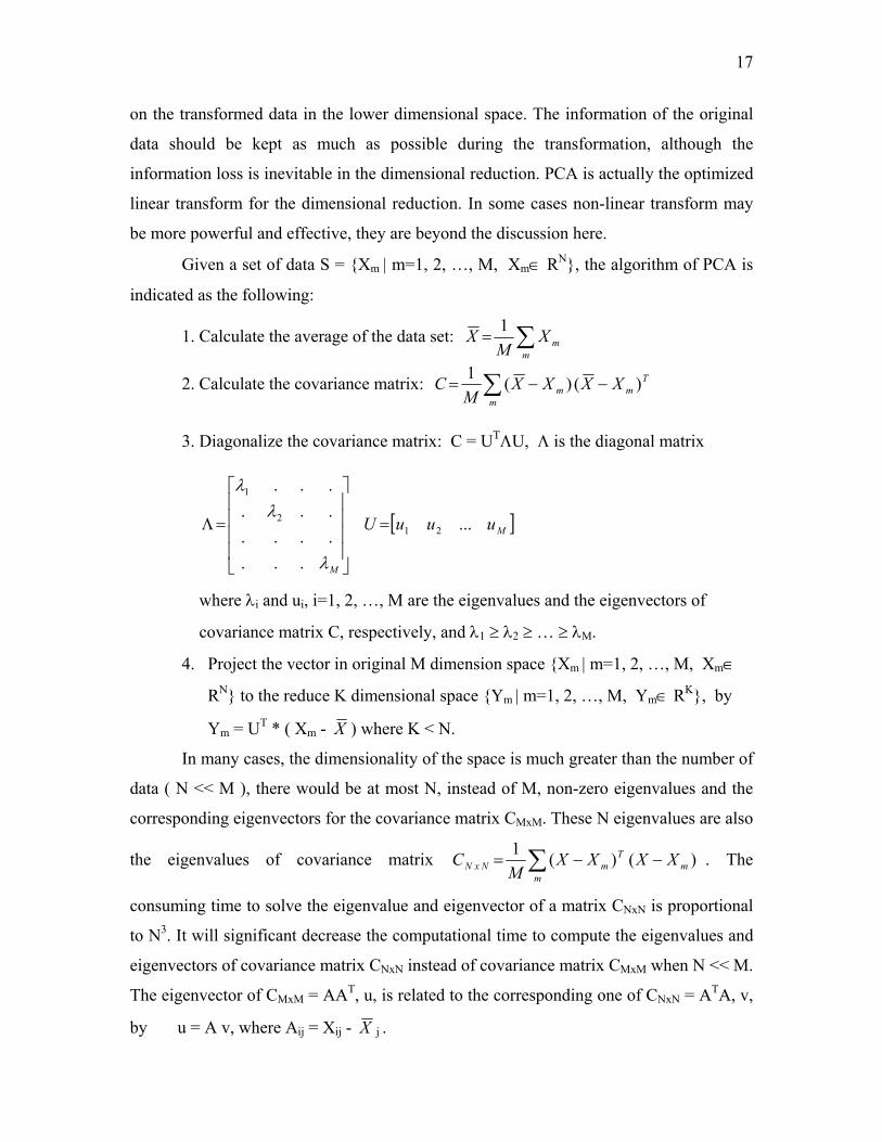
17

on the transformed data in the lower dimensional space. The information of the original

data should be kept as much as possible during the transformation, although the

information loss is inevitable in the dimensional reduction. PCA is actually the optimized

linear transform for the dimensional reduction. In some cases non-linear transform may

be more powerful and effective, they are beyond the discussion here.

Given a set of data S = {Xm | m=1, 2, …, M, Xm∈ RN}, the algorithm of PCA is

indicated as the following:

1. Calculate the average of the data set: ∑=m

mXM

X 1

2. Calculate the covariance matrix: Tm

mm XXXX

MC )()(1

−−= ∑

3. Diagonalize the covariance matrix: C = UTΛU, Λ is the diagonal matrix

[ ]M

M

uuuU ...

.............

212

1

=

=Λ

λ

λλ

where λi and ui, i=1, 2, …, M are the eigenvalues and the eigenvectors of

covariance matrix C, respectively, and λ1 ≥ λ2 ≥ … ≥ λM.

4. Project the vector in original M dimension space {Xm | m=1, 2, …, M, Xm∈

RN} to the reduce K dimensional space {Ym | m=1, 2, …, M, Ym∈ RK}, by

Ym = UT * ( Xm - X ) where K < N.

In many cases, the dimensionality of the space is much greater than the number of

data ( N << M ), there would be at most N, instead of M, non-zero eigenvalues and the

corresponding eigenvectors for the covariance matrix CMxM. These N eigenvalues are also

the eigenvalues of covariance matrix )()(1m

m

TmNxN XXXX

MC −−= ∑ . The

consuming time to solve the eigenvalue and eigenvector of a matrix CNxN is proportional

to N3. It will significant decrease the computational time to compute the eigenvalues and

eigenvectors of covariance matrix CNxN instead of covariance matrix CMxM when N << M.

The eigenvector of CMxM = AAT, u, is related to the corresponding one of CNxN = ATA, v,

by u = A v, where Aij = Xij - X j .

18

3.2.2 MKL algorithm PCA is a very powerful method for pattern reconstruction and pattern recognition,

however, it is effective only for data sets that can be simulated with one Gaussian

distribution, which is not the condition for the most practical cases. Considering that the

more general data sets would be more approximated with multiple Gaussian data sets, it

would be natural to apply PCA for each Gaussian distribution of the real data. The

research has demonstrated that this MKL algorithm outperforms the traditional KL

algorithm, and overcomes the linear problem and scalability problem in some degrees for

both pattern reconstruction and pattern recognition. How the original data should be

partitioned several subspaces properly becomes critical for this MKL approach.

A simple heuristic approach to determine the optimal MKL partition was

proposed as follows: For the given data set, the maximum relative reconstruction error

ξmax, the maximum dimensionality for the target subspaces kmax, and the maximum

number of subspaces smax, the algorithm iterates the procedure to increase the number of

subspaces s, find the optimal partition for the given s by applying MKL, until find a

optimal partition P* whose relative reconstruction error ξ(P*, s) ≤ ξmax , or s ≤ smax. The

optimal partition for the given number of subspaces is obtained by iteratively optimizing

the initial partitions generated by either iterative-removing method or 2D-alignments

method proposed in the paper.

The proposed approach is simple, however its validity couldn’t be proved. There

is no guarantee for the convergence of these iteration methods, although they may work

well for some artificial data in 2D space. The maximum number of iteration is set in

order to eliminate the oscillatory phenomena. This may lead to the inaccurate results.

Another problem is how to choose the parameters ξmax, kmax, and smax. It is difficult to

have a general rule to choose these parameters. Increasing kmax and decreasing ξmax can

improve the reconstruction accuracy in pattern reconstruction. However this may not be

the case for the pattern recognition. Decreasing ξmax may cause the overfitting and global

correlation problems of the data. The running time is also another problem for this MKL

algorithm. PCA is very time-consuming, and it is used for each iteration. It is indicated

that the time complexity of MKL is a quadratic increase in the number of subspaces with

respect to KL time complexity.

19

The partition of the original data is crucial and the bottleneck for MKL algorithm.

The combination of RP and EM algorithms could give a clear and easy approach to

partition data.

3.2.3 RP-EM-MKL algorithm Considering that any data set can be approximated with Gaussian mixtures, MKL

may be a better alternative for pattern reconstruction and recognition for a general data

set. Partitioning the data is the most important step in MKL. The combination of random

projection and expectation maximization is used to partition the data. This algorithm is

very simple and straightforward. The random projection is applied to the original data to

reduce the data dimensionality, then the expectation maximization algorithm is applied to

the data with the reduced dimensionality to partition the data, finally PCA is applied for

each set. This chapter mainly focuses on pattern recognition.

The effectiveness of this combined algorithm is due to the fact that random

projection will keep the separation of Gaussian mixtures in very low dimensional space.

The dimensionality of the low dimensional space depends only on the number of

Gaussian mixtures, and it is independent on the dimensionality of the original data.

Actually the 2-D alignment approach is similar to the random projection, except the 2-D

alignment approach may suffer from the problem when the dimensionality reduction (n

→ 2) may cause severe changes in the data topology, while random projection would

keep the data topology during the dimensionality reduction.

The RP-EM-MKL algorithm is implemented in the following:

1. Reduce the dimensionality by RP algorithm;

2. Apply EM algorithm to partition the data into several Gaussian distributions in

lower dimensional space;

3. Apply MKL algorithm for the data with the partition given by EM algorithm.

The RP algorithm is simple. Given a N x M matrix X = {xij} representing a set of

M N-dimensional vectors, for example each column xi represents an image, the random

projection to reduce the dimensionality can be applied by

Y = R * X

where Y is the K x M matrix representation in the lower dimensionality space, R is a

20

randomly generated K x N orthogonal matrix, which means

R * RT = I K x K

and K is the dimensionality of random projection subspace, K << N

If we assumed that the original set X={xi∈ℜN | i=1, 2, …, M} could be

approximated with the mixtures of k Gaussians, the random projection assures that these

Gaussian mixtures are still separable in the reduced space Y = { yi∈ℜK | i=1, 2, …, m} in

which K could be as low as O(lnk), and K is only dependent on the number of Gaussian

k, and independent on the original dimensionality N. The partition in the lower

dimensionality space can represent the distributions in the higher dimensionality space.

Expectation-maximization algorithm can be applied to partition the data in the reduced

dimensional space.

EM is an algorithm that has the solid mathematics foundation. If the data can be

approximated by Gaussian mixtures, the conditional density of a vector yi modeled as a

Gaussian mixture with K components P (yi ) is:

∑=

Σ=K

kkkkii ypyP

1

),|()( πµ

and each component p(yi | µk, Σk )is approximated as a Gaussian:

])()(21[exp

||21),|( 1

2/1 µµπ

µ kikkiT

kkki yyyp −Σ−−

Σ=Σ −

The parameters for the Gaussian mixture: the coefficiencies πk, and the means µk and

covariance matrices Σk of Gaussian distributions, can be obtained via the standard

expectation and maximization procedures:

Expectation step:

∑=

Σ

Σ= K

j

tk

tj

tji

tk

tk

tki

ik

yp

ypzE

1),|(

),|()(

πµ

πµ

Maximization step:

∑=+

yiik

t

k zEn

)(11π

Ttki

tki

yiikt

k

tk yyzE

n)()()(1 11

11 µµ

π++

++ −−=Σ ∑

21

The expectation and maximization steps are iterated until the convergence meets.

3.3 Experimental data sets There are two data sets used in our experiment. The first data set was obtained

from the author of MKL paper. There are total 90 persons, each individual has 4 original

images. In order to make the data set big enough, 10 derived images are generated from

each original image by a small rotation and transformation distortion. So there are total

90 x (40 + 4) = 3960 images. In the experiment, the individual is randomly selected from

these 90 persons each time, and all the original 4 images for each selected person are also

selected. These selected images for each person are separated as two parts: training set

and testing set. For each individual, 2 original images are randomly selected for testing,

other 2 original images and 2 or 5 derived images for each original image are selected for

training. So for each person, there are 2 images for testing, and 10 or 22 images for

training. The dimension of each image is 55 * 75 = 4125.

The second data set is the ORL data set. There are 40 persons and each individual

has 10 images. There are total 40 x 10 = 400 images. In the experiments, 7 images are

used for training and other 3 images are used for testing for each person. The dimension

of each image is 92 * 112 = 10304.

The scoring recognition rate is used to measure the recognition performance. If

there are n images used for training, the n images which are the nearest to the testing

image are selected. The average correct recognition rate of these nearest n images is the

scoring recognition rate. Sometimes the recognition rate obtained from the average of the

nearest image is also used.

3.4 Experimental Results

3.4.1 The comparison between PCA and RP Theoretically both PCA and RP are orthogonal transformation, in which the

orthogonal matrix is composed of the eigen-vectors corresponding to the largest eigen-

values of covariance matrix of averaged data in PCA, while the orthogonal matrix is

randomly generated in RP. The reconstruction error should be smaller using PCA than

using RP. However this is not the case for pattern recognition, the eigen-vectors

corresponding to the larger eigen-values of the covariance matrix may not be the best

22

choice for the recognition. RP may be a good alternative. Considering that the time

complexity of PCA is O(n3) while it is O(n2m) for RP, m << n, RP would be more

attractive if it can have the comparable recognition rate with that of PCA due to the

running time.

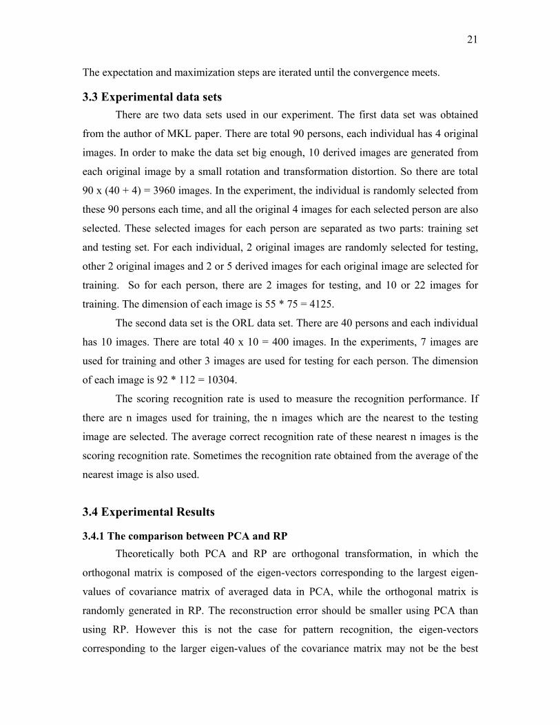
Figures 3.1(a) and 3.1(b) show the scoring recognition rate of PCA and RP with

90 persons and 20 persons, respectively, Figure 3.1(c) and 3.1(d) show the closest

recognition rate of PCA and RP with 90 persons and 20 persons, respectively. 22 and 10

images are randomly selected for the training for each person, and the results are the

average of 50 experiments. All the cases indicate that PCA outperforms RP in lower

dimensional projection space, and RP outperforms PCA in higher dimensional projection

space. The recognition rate will be stable or decrease a little when the dimensionality is

high enough. Considering the time complexity, RP may be a good alternative to PCA for

recognition in high dimensional subspace.

3.4.2 RP-EM-MKL The main purpose of this project is to test whether RP-EM algorithm could be

used as an easy and valid partition approach applied in MKL. Figures 3.2, 3.3, and 3.4

show the RP-EM-MKL results for data set 1, and Figures 3.5, 3.6, 3.7 and 3.8

demonstrate the RP-EM-MKL results for data set 2. All the experiments are the average

of 10 tests. The dimensionality of the PCA in each subgroup of MKL is 1 through 20

with an increment of 1.

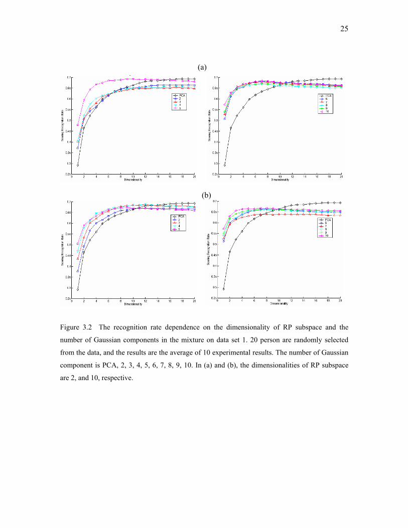
Figures 3.2(a) and 3.2(b) demonstrate the general recognition rate depending on

the dimensionality of RP subspace and the number of Gaussian components in the

mixture. The numbers of Gaussian components are 1 through 10 by increment of 1, and

the dimensionality of RP subspace are 2 are 10 for Figure 3.2(a) and Figure 3.2(b),

respectively. 20 persons were selected and 22 images for each person are used for

training. In lower dimensionality of PCA(d<10), RP-EM-PCA outperform PCA

significantly. RP-EM-PCA reaches its stable level very quickly (around d=6~8), which

means less running time would be need for this algorithm. Although the recognition rate

normally increases when increasing the number of Gaussian components, the results

indicate that 4 or 5 Gaussian components may be enough for this 20 person experiment.

The recognition rate depends less on the dimensionality of RP projection space.

23

Dimensionality as low as 2 still works well. The recognition rate doesn’t change much

when the number of Gaussian components is greater than 5 for dimensionalities of RP

projection space in the range of 2 through 10.

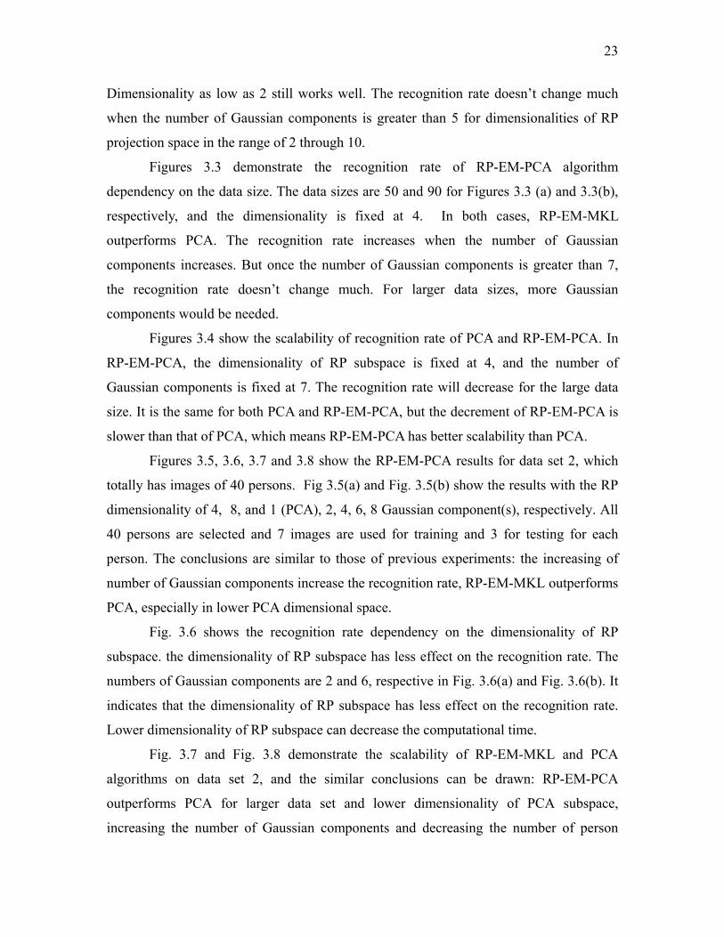
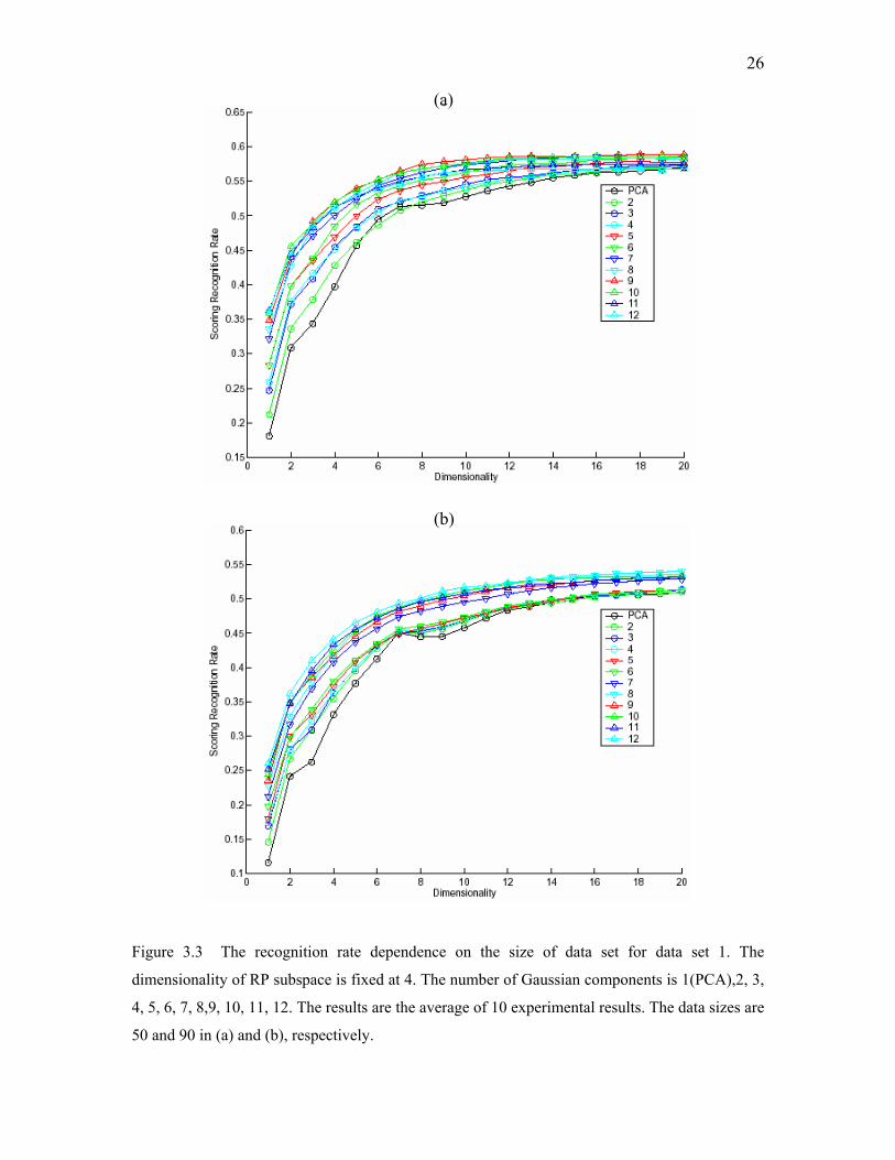
Figures 3.3 demonstrate the recognition rate of RP-EM-PCA algorithm

dependency on the data size. The data sizes are 50 and 90 for Figures 3.3 (a) and 3.3(b),

respectively, and the dimensionality is fixed at 4. In both cases, RP-EM-MKL

outperforms PCA. The recognition rate increases when the number of Gaussian

components increases. But once the number of Gaussian components is greater than 7,

the recognition rate doesn’t change much. For larger data sizes, more Gaussian

components would be needed.

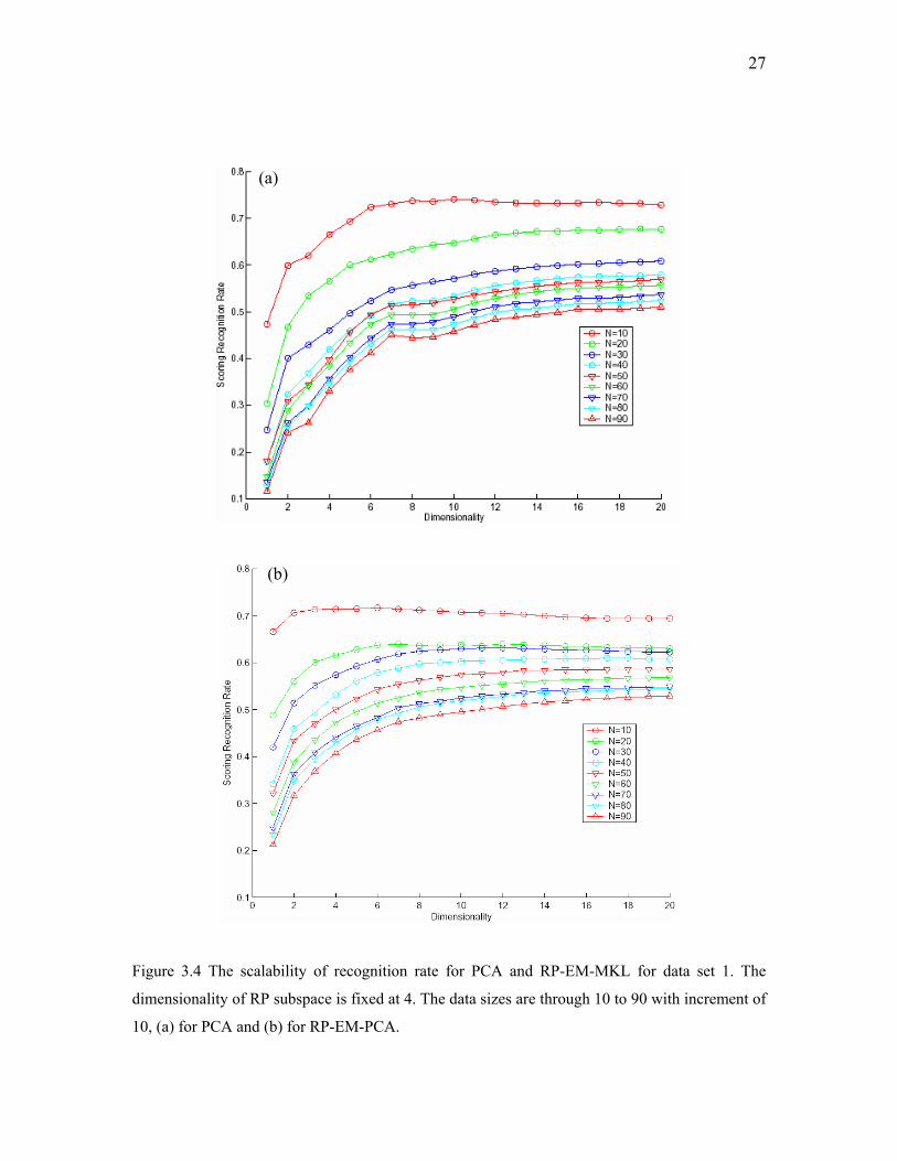
Figures 3.4 show the scalability of recognition rate of PCA and RP-EM-PCA. In

RP-EM-PCA, the dimensionality of RP subspace is fixed at 4, and the number of

Gaussian components is fixed at 7. The recognition rate will decrease for the large data

size. It is the same for both PCA and RP-EM-PCA, but the decrement of RP-EM-PCA is

slower than that of PCA, which means RP-EM-PCA has better scalability than PCA.

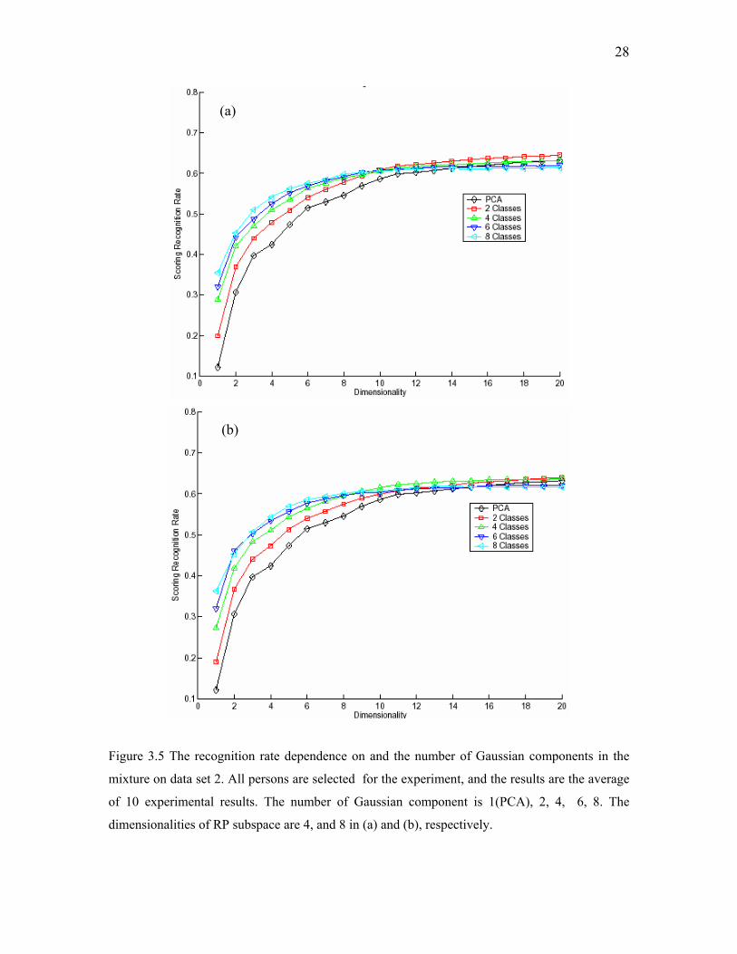
Figures 3.5, 3.6, 3.7 and 3.8 show the RP-EM-PCA results for data set 2, which

totally has images of 40 persons. Fig 3.5(a) and Fig. 3.5(b) show the results with the RP

dimensionality of 4, 8, and 1 (PCA), 2, 4, 6, 8 Gaussian component(s), respectively. All

40 persons are selected and 7 images are used for training and 3 for testing for each

person. The conclusions are similar to those of previous experiments: the increasing of

number of Gaussian components increase the recognition rate, RP-EM-MKL outperforms

PCA, especially in lower PCA dimensional space.

Fig. 3.6 shows the recognition rate dependency on the dimensionality of RP

subspace. the dimensionality of RP subspace has less effect on the recognition rate. The

numbers of Gaussian components are 2 and 6, respective in Fig. 3.6(a) and Fig. 3.6(b). It

indicates that the dimensionality of RP subspace has less effect on the recognition rate.

Lower dimensionality of RP subspace can decrease the computational time.

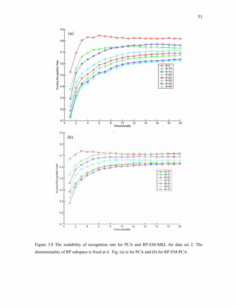
Fig. 3.7 and Fig. 3.8 demonstrate the scalability of RP-EM-MKL and PCA

algorithms on data set 2, and the similar conclusions can be drawn: RP-EM-PCA

outperforms PCA for larger data set and lower dimensionality of PCA subspace,

increasing the number of Gaussian components and decreasing the number of person

24

increase the recognition rate, and RP-EM-MKL has the better scalability than PCA.

(a) (b)

(c) (d)

Figure 3.1 The comparison of scoring recognition rate and closest recognition rate between RP

and PCA with 90 and 20 individuals. (a): the scoring recognition rate with 90 individuals, (b): the

scoring recognition rate with 20 individuals, 3.1(c): the closest recognition rate with 90

individuals, 3.1(d): the closet recognition rate with 20 individuals. In each case, PCA and RP

were performed with 22 images or 10 images as the train individually.

25

(a)

(b)

Figure 3.2 The recognition rate dependence on the dimensionality of RP subspace and the

number of Gaussian components in the mixture on data set 1. 20 person are randomly selected

from the data, and the results are the average of 10 experimental results. The number of Gaussian

component is PCA, 2, 3, 4, 5, 6, 7, 8, 9, 10. In (a) and (b), the dimensionalities of RP subspace

are 2, and 10, respective.

26

(a)

(b)

Figure 3.3 The recognition rate dependence on the size of data set for data set 1. The

dimensionality of RP subspace is fixed at 4. The number of Gaussian components is 1(PCA),2, 3,

4, 5, 6, 7, 8,9, 10, 11, 12. The results are the average of 10 experimental results. The data sizes are

50 and 90 in (a) and (b), respectively.

27

(a)

(b)

Figure 3.4 The scalability of recognition rate for PCA and RP-EM-MKL for data set 1. The

dimensionality of RP subspace is fixed at 4. The data sizes are through 10 to 90 with increment of

10, (a) for PCA and (b) for RP-EM-PCA.

28

(a)

(b)

Figure 3.5 The recognition rate dependence on and the number of Gaussian components in the

mixture on data set 2. All persons are selected for the experiment, and the results are the average

of 10 experimental results. The number of Gaussian component is 1(PCA), 2, 4, 6, 8. The

dimensionalities of RP subspace are 4, and 8 in (a) and (b), respectively.

29

(a)

(b)

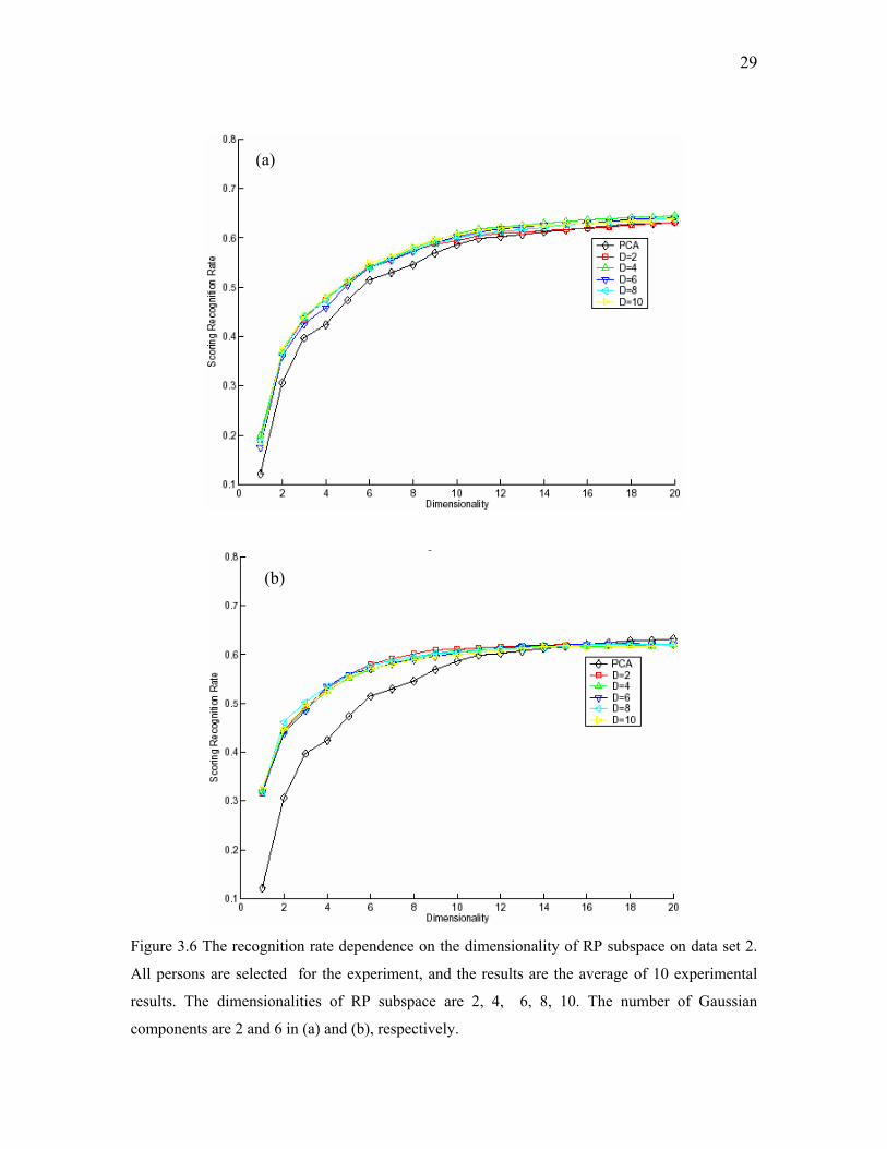
Figure 3.6 The recognition rate dependence on the dimensionality of RP subspace on data set 2.

All persons are selected for the experiment, and the results are the average of 10 experimental

results. The dimensionalities of RP subspace are 2, 4, 6, 8, 10. The number of Gaussian

components are 2 and 6 in (a) and (b), respectively.

30

(a)

(b)

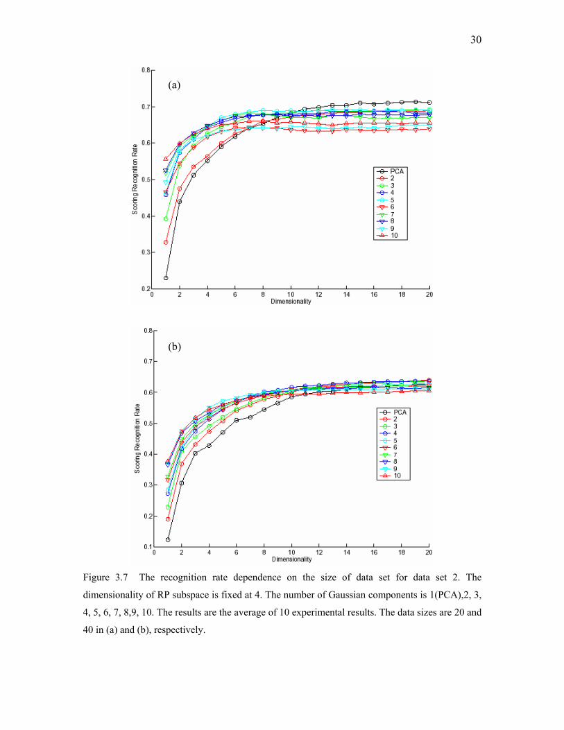
Figure 3.7 The recognition rate dependence on the size of data set for data set 2. The

dimensionality of RP subspace is fixed at 4. The number of Gaussian components is 1(PCA),2, 3,

4, 5, 6, 7, 8,9, 10. The results are the average of 10 experimental results. The data sizes are 20 and

40 in (a) and (b), respectively.

31

(a)

(b)

Figure 3.8 The scalability of recognition rate for PCA and RP-EM-MKL for data set 2. The

dimensionality of RP subspace is fixed at 4. Fig. (a) is for PCA and (b) for RP-EM-PCA.

32

3.5 Conclusions The combination of random projection (RP) and expectation maximization (EM)

algorithms was proposed as an approach to partition the data set in multispace KL (MKL)

for pattern recognition. The proposed approach is solid, very easy to understand and

implement. This ease of implementation is due to the fact that expectation maximization

algorithm has been proved powerful enough to partition the Gaussian mixture datasets,

and the random projection algorithm can reduce the dimensionality effectively while

keeping the separable property of the data. The experimental results on several data sets

indicated that this RP-EM-MKL algorithm could ease the complexity of MKL by

decrease the number of parameters to be chosen, save the computing time, outperform

KL (PCA) in lower dimensional PCA projection space and larger data sets, and still have

good scalability.

33

Chapter 4

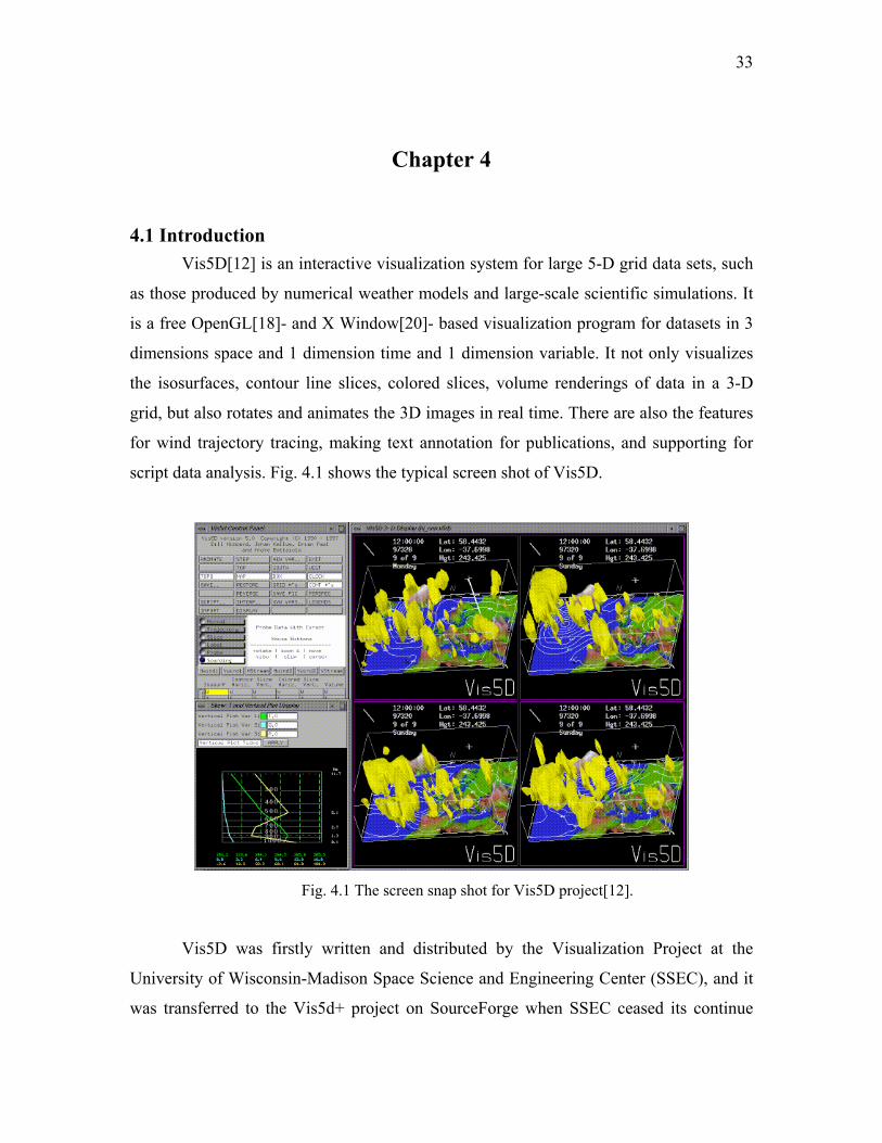
4.1 Introduction Vis5D[12] is an interactive visualization system for large 5-D grid data sets, such

as those produced by numerical weather models and large-scale scientific simulations. It

is a free OpenGL[18]- and X Window[20]- based visualization program for datasets in 3

dimensions space and 1 dimension time and 1 dimension variable. It not only visualizes

the isosurfaces, contour line slices, colored slices, volume renderings of data in a 3-D

grid, but also rotates and animates the 3D images in real time. There are also the features

for wind trajectory tracing, making text annotation for publications, and supporting for

script data analysis. Fig. 4.1 shows the typical screen shot of Vis5D.

Fig. 4.1 The screen snap shot for Vis5D project[12].

Vis5D was firstly written and distributed by the Visualization Project at the

University of Wisconsin-Madison Space Science and Engineering Center (SSEC), and it

was transferred to the Vis5d+ project on SourceForge when SSEC ceased its continue

34

development on Vis5D. Vis5d+ is based on Vis5d version 5.2, and it is intended as a

central repository for enhanced versions and development work on Vis5D.

The package I worked on is the latest version (1.2.0) of Vis5d+, which was

released in November 1, 2001. It makes some modifications to vis5d 5.2, such as

• Support for stereo display mode,

• Support for scene output to VRML format.

• Improved screen image dumping.

• Improved Isosurface rendering using decimated meshes

• Many structures and arrays have been changed from statically to dynamically

allocated.

• They also began to add graphic user interface (GUI) based on gtk+ (this is not

finished)

Although Vis5d is very powerful, there are some distinct drawbacks which make

it less useful in many cases, especially when some modifications need to be made:

1 The project was created about 10 years ago in which time very fewer tool kits are

available. Considering the rapid progresses and new concepts in computer

science, especially in software engineering, Vis5d lacks many advanced features,

such as Model-Viewer-Controller, Object-Oriented, Event-Driven in the original

design. The design was not clear, the defined data structures are complicated and

their inter-relationship is very complex.

2 The interactive graphics user interface (GUI) is based on LUI5 widget package,

which is based on X-Windows directly. X windows system is famous for its easy

usage for the user, but hard to programming for the developer. Currently GUI

toolkits, such as QT, Motif, CDF, are provided to ease those X Windows

programming. However in Vis5d, the developer needs to modify the message

loop to choose the specific user events, and define the corresponding event

handling functions via the callback function concepts.

All of these make it difficult for the developers to port or modify the source code

before the users fully understand the logic and physical structures of the whole package.

However, it is not easy to fully understand the whole package due to the complicated

relationship between each part, and the lacking of documentations for the project. The

35

package is pretty large (source code is about 4MB), and there are very fewer comments

and the documentation written in the source code.

In the project present in this chapter, I was required to extract various data along

the specified flight paths at specific time, and then visualize the extracted data. I tried to

use the original Vis5D and to make some modifications, however it seemed more

difficult to make the modifications on the original source code than to implement Vis5D

from scratch. After several months work, I decide to redesign and re-implement the

Vis5D project making use of some new techniques and tools, such as the Object-Oriented

(OO) and Model/View/Controller (MVC) design pattern[4], and QT tools[19, 16].

Although only the basic functions in Vis5D were implemented in the current project, the

advanced features, such as multi-threading, shared-memory, or even parallel computing

and visualization could be added easily later.

This chapter is organized as the following: the structure and the control flow of

the original Vis5D project will be reviewed first, then the new design for the project is

described, and some screen snapshots are demonstrated, some possible future work is

also listed.

4.2 The Structure of Vis5D The basic idea of Vis5D is very simple: all the data are points in a 5D space (3 for

space coordinate x, y, z, 1 for variable and 1 for time), the data values at the specific time

and variable, and within a region will be visualized by the color or other indicators in the

computer window. The visualized data are stored in a file in Vis5D format. Besides the

Vis5D data, there are topo file to store the topology of the earth or a region on the earth,

and map file to store the 2D map data.

As shown in Figure 4.1, there are two types of windows in Vis5D: left is the

control panel to change the visualization control parameters, and the right is the multiple

(1x1 to 4x4) 3D windows to visualize data and render 2D/3D images. Each 3D window

could visualize different Vis5D data source, or the same Vis5d data source, which was

provided by the corresponding graphics context and data context.

The control flow of Vis5D is shown in Figure 4.2, and the main part is the infinite

loop to waiting for the user input event, which is shown in Figure 4.3:

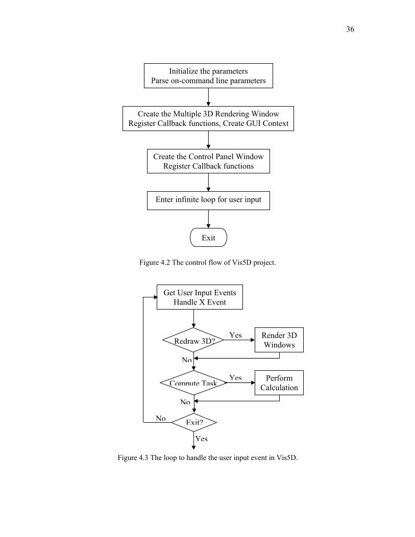
36

Exit

Enter infinite loop for user input

Create the Control Panel WindowRegister Callback functions

Create the Multiple 3D Rendering Window Register Callback functions, Create GUI Context

Initialize the parameters Parse on-command line parameters

Figure 4.2 The control flow of Vis5D project.

No

No

No

Yes

Yes

Yes

Exit?

Compute Task Perform Calculation

Redraw 3D?Render 3D Windows

Get User Input EventsHandle X Event

Figure 4.3 The loop to handle the user input event in Vis5D.

37

There are two main tasks for the visualization: performing the calculation for the

rendering and update the 3D rendering window. These tasks are put in a queue. In the

event handler functions, the tasks need to be performed further are put into the queue

waiting to be performed by the program. The main loop procedure extracts the task from

the task queue, and invokes the corresponding function to complete it.

There are 3 main data sets in Vis5d: Vis5D data, topology data, and map data.

Each has its own format when stored in the file. It is important understand the format the

retrieve the data from the file correctly. The format of Vis5D data will be described in the

following.

The Vis5D data is stored in binary format, the file is composed of three parts: the

signature, the header and the data. The signature of Vis5D data file is “V5d\n”.

The header is composed of several tag/value pairs, it provides the general

information about the whole data in the file, such as the number of variables, variable

units, variable names, the time information, the mapping between the row, column, level

index and the latitude, longitude, and height, etc.. Each one tag/value pair consists of

integer information tag, the integer length of this pair in byte, and the related value. The

meaning of the value is related to the information tag. For example, if the tag is

TAG_NR, the following value is the number of row for the data block, if the tag is

TAG_PROJECTION, the following value is the projection type, which is the mapping

between the level and the height.

The real data values are stored the data part, block by block. Each block of the

data part is the values for one variable at one time and one level, which are the data for

(number of rows) x (number of columns) points at one level. The data stored may be

compressed to reduce the size of the data file. The information about the mapping

between (row, column) and (latitude, longitude), and the compression mode are provided

in the header.

4.3 Design, Implementation and Results In the scientific visualization, a large amount of data needed to analyzed and

visualized. Contrary to the normal structured-oriented or object-oriented patterns, the data

should be emphasized, the data-oriented pattern may be more suitable during the design

38

and the implementation, in which MVC is a good example.

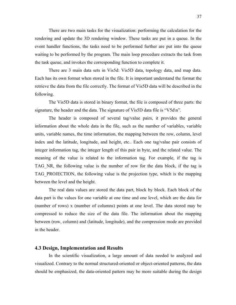
MVC is used widely to build graphics user interface (GUI), where the model is

the application object, the view is the screen presentation, and the controller defines the

way the user interface reacts to user input. A diagram of this is shown in Figure 4.4. In

the current implementation, the QT toolkit is used, the model is the data, original data or

derived data, the view is the frame window, and the controller is provide by the dialog.

View (Frame)

Controller(Dialog)

Model(data)

Figure 4.4 The diagram of MVC.

There are 3 types of data: Vis5D data, topo data, and the map data. Currently the

visualization of map data is not implemented. We have also added the visualization of

values along a specified flight path.

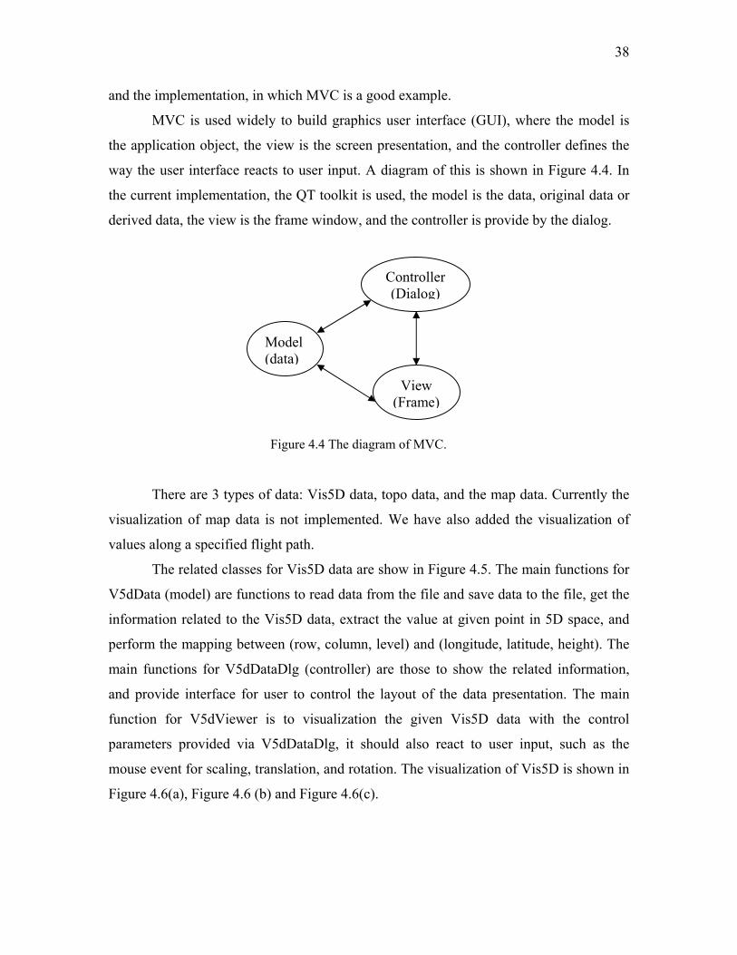
The related classes for Vis5D data are show in Figure 4.5. The main functions for

V5dData (model) are functions to read data from the file and save data to the file, get the

information related to the Vis5D data, extract the value at given point in 5D space, and

perform the mapping between (row, column, level) and (longitude, latitude, height). The

main functions for V5dDataDlg (controller) are those to show the related information,

and provide interface for user to control the layout of the data presentation. The main

function for V5dViewer is to visualization the given Vis5D data with the control

parameters provided via V5dDataDlg, it should also react to user input, such as the

mouse event for scaling, translation, and rotation. The visualization of Vis5D is shown in

Figure 4.6(a), Figure 4.6 (b) and Figure 4.6(c).

39

private data members: V5dData V5dDataParam

view the data with control parameters from V5dDataDlg;

V5dViewer (View)

private data member: V5dData

show data information ; show control parameters (V5dDataParam) for viewing

V5dDataDlg (Controller) read data from a file; save data to a file; get data information ; calculate mapping between (row, column, level) and (longitude, latitude, height); get value at specific point in 5D (row, column, level, time, variable) or (longitude, latitude, height, time, variable);

V5dData (Model)

Figure 4.5 The diagram of the implemented classes for Vis5D data.

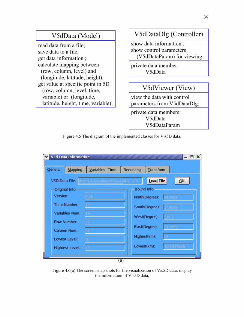
(a)

Figure 4.6(a) The screen snap shots for the visualization of Vis5D data: display the information of Vis5D data,

40

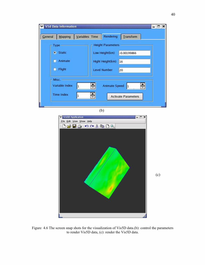
(b)

(c)

Figure 4.6 The screen snap shots for the visualization of Vis5D data.(b): control the parameters to render Vis5D data, (c): render the Vis5D data.

41

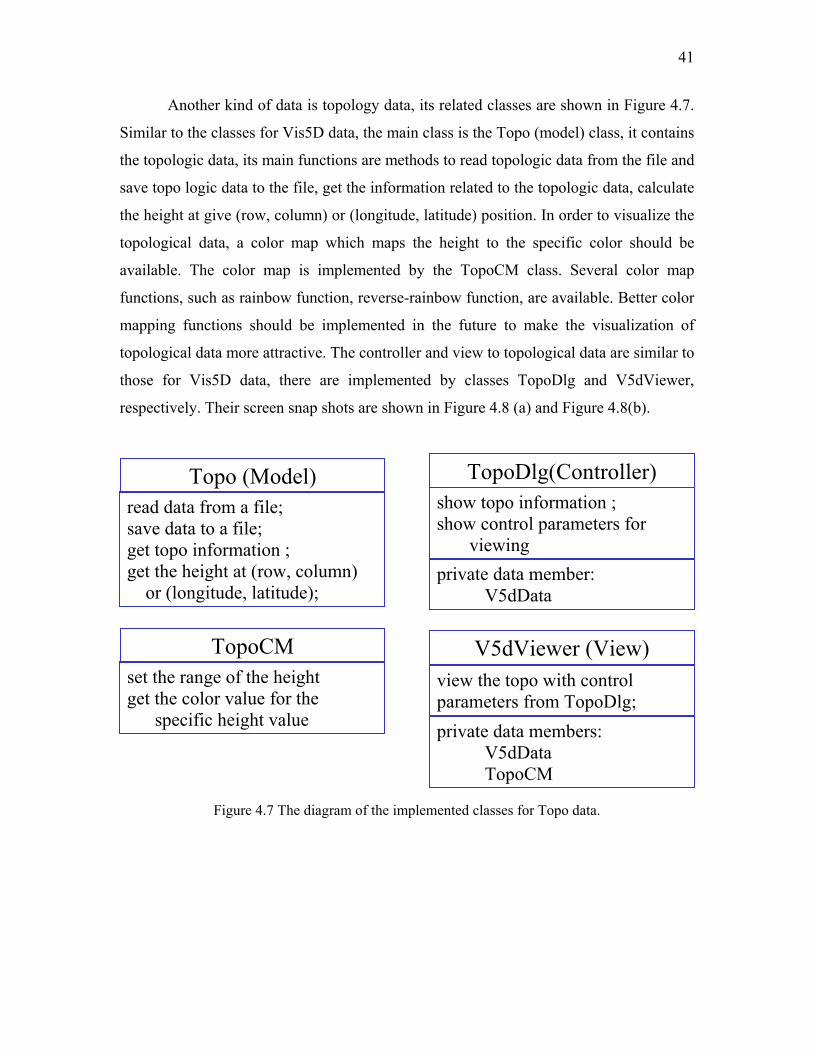
Another kind of data is topology data, its related classes are shown in Figure 4.7.

Similar to the classes for Vis5D data, the main class is the Topo (model) class, it contains

the topologic data, its main functions are methods to read topologic data from the file and

save topo logic data to the file, get the information related to the topologic data, calculate

the height at give (row, column) or (longitude, latitude) position. In order to visualize the

topological data, a color map which maps the height to the specific color should be

available. The color map is implemented by the TopoCM class. Several color map

functions, such as rainbow function, reverse-rainbow function, are available. Better color

mapping functions should be implemented in the future to make the visualization of

topological data more attractive. The controller and view to topological data are similar to

those for Vis5D data, there are implemented by classes TopoDlg and V5dViewer,

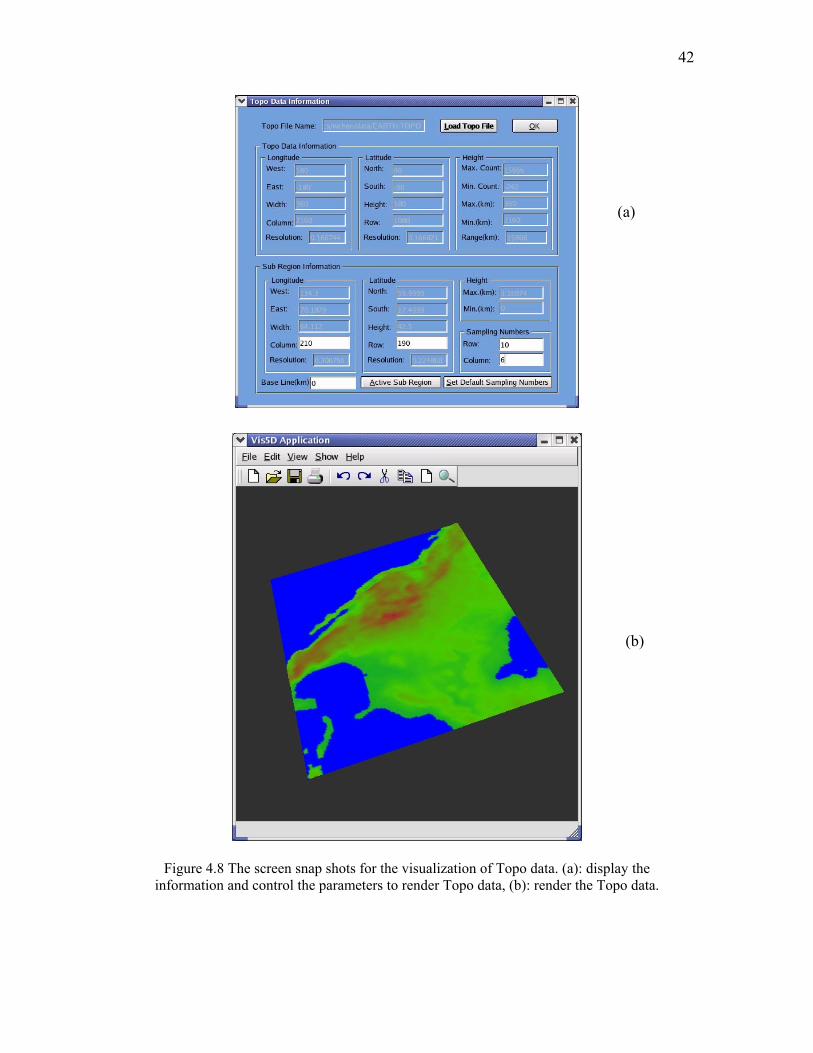
respectively. Their screen snap shots are shown in Figure 4.8 (a) and Figure 4.8(b).

set the range of the height get the color value for the specific height value

TopoCM

private data members: V5dData TopoCM

view the topo with control parameters from TopoDlg;

V5dViewer (View)

private data member: V5dData

show topo information ; show control parameters for viewing

TopoDlg(Controller) read data from a file; save data to a file; get topo information ; get the height at (row, column) or (longitude, latitude);

Topo (Model)

Figure 4.7 The diagram of the implemented classes for Topo data.

42

(a)

(b)

Figure 4.8 The screen snap shots for the visualization of Topo data. (a): display the

information and control the parameters to render Topo data, (b): render the Topo data.

43

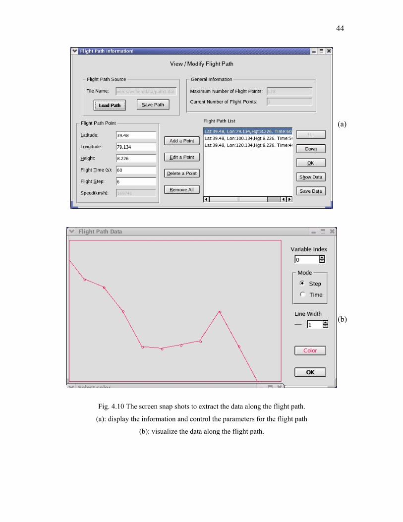
The main task of this chapter is to extract the variable values along a specified

flight path. Its related classes are shown in Figure 4.9. The model is represented by

FlighPath class, which stores information about the flight path, such as the position, time

interval, speed, etc.. Its controller is represented by FPDlg, which provides a GUI to

change and show the flight path information. The visualization of the retrieved data along

the given flight path is implemented by the functions in V5dViewer class. The screen

snap shots for flight path are shown in Figures 4.10(a) and 4.10(b).

set / get flight path data at specific point;

FPData

private data members: V5dData FPData

view the topo with control parameters from TopoDlg;

V5dViewer (View)

private data member: FPData

show Flight Path information ; show control parameters for viewing

FPDlg(Controller) read data from a file; save data to a file; get flight data at specific point;

FlightPath (Model)

Figure 4.9 The diagram of the implemented classes for flight path.

44

(a)

(b)

Fig. 4.10 The screen snap shots to extract the data along the flight path.

(a): display the information and control the parameters for the flight path

(b): visualize the data along the flight path.

45

4.4 Future Work

Although the design and the basic functions for the project have been finished, this project is far from the complement. Much further work needs to be done, such as:

• Implement MVC classes for Map data;

• Add advanced features, such as contours, isosurfaces, contour line slice,

animations;

• Implement multithread and/or parallel computing for background calculations

for advanced features

• Make more attractive interface, improve the color mapping

• Support for other data format

• Export printable images for the outputs

• Documentation

4.5 Conclusions The program based on Qt and OpenGL was designed and implemented to

visualize and extract the data along the specified flight path on the Vis5D data. It was

designed with OOP and MVC to facility the adding of further functions, and its some

basic functions have been implemented and tested.

46

Chapter 5

Conclusions

In this professional paper, the work in the different areas of Computer Science has

been present: parallel computing, pattern recognition, and scientific data visualization:

In Chapter 2, parallel computing is applied to solve the problem in the simulation

of N2 and NO collision system. The parallel program with MPI is implemented and

applied for the simulation, and it significantly reduces the waiting time to obtain the

simulation results. The results indicate that parallel computing is very suitable for this

kind nearly embarrassingly problems. High speedup and efficiency are obtained for the

parallel implementation.

In Chapter 3, the combination of random projection (RP) and expectation

maximization (EM) algorithms was proposed as an approach to partition the data set in

multispace KL (MKL) for pattern recognition. The proposed approach is solid, very easy

to understand and implement. This ease of implementation is due to the fact that

expectation maximization algorithm has been proved powerful enough to partition the

Gaussian mixture datasets, and the random projection algorithm can reduce the

dimensionality effectively while keeping the separable property of the data. The

experimental results on several data sets indicated that this RP-EM-MKL algorithm could

ease the complexity of MKL by decrease the number of parameters to be chosen, save the

computing time, outperform KL (PCA) in lower dimensional PCA projection space and

larger data sets, and still have good scalability.

In Chapter 4, the program based on Qt and OpenGL to was designed and

implemented to visualize and extract the data from Vis5D data file. The program was

designed with OOP and MVC to facility the adding of further functions, and some basic

functions have been implemented and tested.

47

Bibliography [1] R. Cappelli, and D. Maio, Multispace KL for Pattern Representation and

Classification, IEEE Trans. Pattern Analysis and Machine Intelligence, Vol 23, No. 9, p977-996, 2001.

[2] S. Dasgupta, Learning mixtures of Gaussians, 40th Annual IEEE Symp. On

Foundations of Computer Science, p634-644, 1999. [3] S. Dasgupta, Experiments with random projection, Proc. Uncertainty in Artificial

Intelligence, 2000. [4] Erich Gamma, Richard Helm, Ralph Johnson, John Vlissides, Design Patterns,

Elements of Reusable Object-Oriented Software, Addison-Wesley, (Reading, MA,) 1995.

[5] K. Karhynen, Uber Lineare Methoden in der Wahrscheinkichkeitsrechung, Ann.

Academy Science Fennicae, Vol. 37, p3-79, 1946. [6] K.T. Lorenz, D.W. Chandler, J.W. Barr, W. Chen, G.L. Barnes, and J.I. Cline, Direct

measurement of the preferred sense of NO rotation after collision with argon, Science, Vol. 293, p2063-2066 , 2001.

[7] T. Mitchell, Machine Learning, McGraw-Hill, 1997. [8] T. Moon, The Expectation-Maximization Algorithm, IEEE Signal Processing

Magazine, Nov. 1996. [9] M. Turk and A. Pentland, Eigenfaces for Recognition, J. of Cognitive Neuroscience,

Vol. 3, No.1, p71-86, 1991 [10] Amber Home Page. A set of molecular mechanical force fields for the simulation of

biomolecules and a package of molecular simulation programs. Available on the web: http://amber.scripps.edu/ Accessed July 10, 2003.

[11] MPQC Web Page. The Massively Parallel Quantum Chemistry Program. Available

on the web: http://aros.ca.sandia.gov/~cljanss/mpqc/ Accessed July 10, 2003. [12] Vis5D+ Web Page. A free OpenGL-based volumetric visualization program for

scientific datasets in 3+ dimensions. Available on the web: http://vis5d.sourceforge.net/ Accessed July 10, 2003.

[13] Massive Parallelism: The Hardware for Computational Chemistry? Available on the

web: http://www.dl.ac.uk/CCP/CCP1/parallel/MPP/mpp.html Accessed July 10, 2003.

[14] NWChem Web page. A computational chemistry package that is designed to run on

high-performance parallel supercomputers as well as conventional workstation

48

clusters. Available on the web: http://www.emsl.pnl.gov:2080/docs/nwchem/ nwchem.html Accessed July 10, 2003.

[15] Gaussian.com. Gaussian series of electronic structure programs. Available on the

web: http://www.gaussian.com Accessed July 10, 2003. [16] libQGLViewer. A GPL free software C++ library which lets you quickly start the

development of a new 3D application. Available on the web: http://www-imagis.imag.fr/ Membres/Gilles.Debunne/CODE/ QGLViewer Accessed July 10, 2003.

[17] GAMESS. The General Atomic and Molecular Electronic Structure System

(GAMESS), a general ab initio quantum chemistry package. Available on the web: http://www.msg.ameslab.gov/GAMESS/GAMESS.html Accessed July 10, 2003.

[18] OpenGL. The premier environment for developing portable, interactive 2D and 3D

graphics applications. Available on the web: http://www.opengl.org/ Accessed July 10, 2003.

[19] Trolltech company. A company to develop multiplatform application development

frameworks and a comprehensive embedded Linux application platform for PDAs and other mobile devices. Available on the web: http://www.trolltech.com/ Accessed July 10, 2003.

[20] X.Org. The worldwide consortium empowered with the stewardship and

collaborative development of the X Window System technology and standards. Available on the web: http://www.X.org/ Accessed July 10, 2003.