PARALLEL ALGORITHMS FOR ROBUST …ufdcimages.uflib.ufl.edu/UF/00/09/46/60/00001/JCA2001.pdfPARALLEL ALGORITHMS FOR ROBUST BROADBAND MVDR BEAMFORMING PRIYABRATA SINHA, ALAN D. GEORGE

© 2000 Univ. of Florida. All Rights Reserved.

PARALLEL ALGORITHMS FOR ROBUST BROADBAND MVDR BEAMFORMING

PRIYABRATA SINHA, ALAN D. GEORGE and KEONWOOK KIM

High-performance Computing and Simulation (HCS) Research Laboratory Department of Electrical and Computer Engineering, University of Florida

P.O. Box 116200, Gainesville, FL 32611-6200

Rapid advancements in adaptive sonar beamforming algorithms have greatly increased the computation and communication demands on beamforming arrays, particularly for applications that require in-array autonomous operation. By coupling each transducer node in a distributed array with a microprocessor, and networking them together, embedded parallel processing for adaptive beamformers can significantly reduce execution time, power consumption and cost, and increase scalability and dependability. In this paper, the basic narrowband Minimum Variance Distortionless Response (MVDR) beamformer is enhanced by incorporating broadband processing, a technique to enhance the robustness of the algorithm, and speedup of the matrix inversion task using sequential regression. Using this Robust Broadband MVDR (RB-MVDR) algorithm as a sequential baseline, two novel parallel algorithms are developed and analyzed. Performance results are included, among them execution time, scaled speedup, parallel efficiency, result latency and memory utilization. The testbed used is a distributed system comprised of a cluster of personal computers connected by a conventional network.

1. Introduction

A beamformer is a spatial filter that processes the data obtained from an array of sensors in a manner that serves to enhance the amplitude of the desired signal wavefront relative to background noise and interference. Beamforming algorithms are the foundation for all array signal processing techniques. Here, the application of beamforming techniques in the area of underwater sonar processing using a linear array of uniformly spaced hydrophones is being considered. The desired function of the beamforming system is to perform spatial filtering of the data in order to find the direction of arrival (DOA) of the target signal, while maintaining a high signal-to-noise ratio (SNR) in the output.

The simplest approach to beamforming is Conventional Beamforming (CBF).1-2 In CBF, signals sampled across an array are linearly phased by complex-valued steering vectors. Thus, the normalized steering or delay vectors by themselves serve as weight vectors. These weights are constant and independent of the incoming data. By contrast, Adaptive Beamforming (ABF) algorithms correlate the weight vectors with the incoming data so as to optimize the weight vectors for high-resolution DOA detection in a noisy environment. Such algorithms use the properties of the Cross-Spectral Matrix (CSM) in order to reject interference from other sources and sensor noise and isolate the true source directions accurately. There are various ABF algorithms proposed in the literature.3-7 Castedo et al.4 proposed a method based on gradient-based iterative search that makes use of properties of cyclostationary signals. Krolik et al.5 defined a steered covariance matrix as an efficient space-time statistic for high-resolution bearing estimation in broadband settings. The algorithm considered here is the MVDR algorithm described by Cox et al.6 MVDR is an optimal technique that selects the weights in such a way that the output power is minimized, subject to the constraint that the gain in the steering direction being considered is unity. This optimization of the weights leads to effective interference-rejection capabilities, as nulls are steered in


2

directions of strong interference. Wax and Anu8 presented an analysis of the signal-to-interference-plus-noise ratio (SINR) at the output of the minimum variance beamformer. Raghunath and Reddy9 analyzed the finite-data performance of the MVDR beamformer. Zoltowski10 developed expressions that describe the output of the MVDR beamformer in the presence of multiple correlated interfering signals. Harmanci et al.11 derived a maximum likelihood spatial estimation method that is closely related to minimum variance beamforming.

However, classical MVDR beamforming techniques suffer from problems of signal suppression in the presence of errors such as uncertainty in the look direction and array perturbations. To mitigate such problems, various constrained MVDR beamforming schemes have been proposed in the literature. These schemes enhance the robustness of the MVDR algorithm. White noise injection based on a white noise gain constraint (WNGC) was described by Cox et al.6 They also described an alternative method known as Cox Projection WNGC that is based on a decomposition of the ABF weight vector into two orthogonal components. Applebaum and Chapman12 demonstrated various methods of preventing signal cancellation problems, using constraints on the main beam. Takao et al.13 introduced constraints on the response to specified directions. Additional constraints on the beamformer response, known as derivative constraints, were presented and analyzed by Er and Cantoni.14

It has been observed in recent years that the aforementioned advancements in beamforming algorithms are placing a tremendous computational load on traditional sonar array systems. This increase in computational requirements makes it imperative to consider and apply parallel processing techniques to sonar beamforming. Besides the substantial computational resources required by these algorithms, it is also necessary to ensure that the performance of the algorithms scales with problem and system size. To this end, various parallel beamforming schemes have been studied in the literature, and much of this research has assumed systolic array systems.15-20 However, despite the performance capabilities of such systems, they are statically implemented on special-purpose processors built using VLSI techniques, and are thus not dynamically configurable with change in the problem size. Moreover, the algorithms in such systems are closely coupled to the systolic array architecture and cannot be efficiently executed on general-purpose distributed systems due to high communication requirements.

Keeping the objective of scalability in view, loosely coupled distributed systems provide a promising alternative. Three parallel algorithms for CBF in the frequency domain were developed and analyzed by George et al.21 Two parallel algorithms for Split-Aperture Conventional Beamforming (SA-CBF), one coarse-grained and the other medium-grained, were presented by George and Kim.22 Parallel algorithms for three different beamforming methods were compared by Kim et al.23,24 A fine-grained parallel algorithm for MVDR beamforming was proposed by Banerjee and Chau.25 However, fine-grained parallelization techniques are not deemed suitable for loosely coupled distributed architectures due to the frequent instances of communication required by such algorithms. This problem was addressed by George et al.26 with a set of parallelization techniques for adaptive beamforming algorithms. A narrowband MVDR beamformer without robustness constraints was used as a baseline to investigate the efficiency and effectiveness of the methods in an experimental fashion. The execution of different beamforming iterations was performed in a pipelined manner by the different processing nodes, while each phase of the MVDR algorithm was partitioned across pipeline stages.

Inversion of the CSM has been observed to be one of the most computationally expensive stages of the MVDR algorithm, and it is thus necessary to improve the computational efficiency of the matrix inversion task. Various methods of matrix inversion are described in the literature,27-29 and much work exists in the area of parallel matrix inversion.30-35 However, these are fine-grained methods involving frequent inter-processor communication, and are thus not suitable for distributed processing systems which typically have a large communication overhead. George et al.26 used a matrix inversion technique based on Gauss-Jordan elimination with full pivoting. In the Gauss-Jordan elimination method, the transformation of each column


3

of the CSM is performed independently of every other column. The transformation of the entire CSM could therefore be conveniently partitioned across pipeline stages, with each column being processed in a different pipeline stage.

The work presented in this paper extends the work of George et al.26 in two significant ways. First, the basic narrowband sequential MVDR algorithm has been extended by the addition of three features: broadband processing, speedup of the matrix inversion stage of the algorithm using a sequential regression technique, and a technique to enhance the robustness of the algorithm. The various stages of the resulting RB-MVDR algorithm have been analyzed in terms of computational and memory requirements in order to provide a foundation for the design of efficient parallelization techniques. The second, and most significant, contribution of this research is the development of two novel distributed parallel algorithms for RB-MVDR beamforming.

The first parallel algorithm presented in this paper is a Frequency Decomposition (FD) technique, in which each processor handles a different set of frequency bins, and an averaging operation is performed at the end to obtain the final output. This method requires an all-to-all communication pattern to distribute the data to all the nodes on the basis of frequency.

The second parallel algorithm is a novel variant of the iteration decomposition techniques presented by George and Kim22 and George et al.26 In this scheme, called the Frequency-pipelined Iteration Decomposition (FID), successive beamforming iterations are overlapped and executed in a round-robin fashion by different processing nodes. Thus, while a processor is processing the data collected from each sensor in the array at a given time, all the other nodes are concurrently performing beamforming iterations with data sets collected at different times. Within each iteration, the processing of different frequency bands is partitioned across different pipeline stages. This scheme involves all-to-one communication.

An overview of basic narrowband MVDR is presented in Section 2. A theoretical overview of RB-MVDR, with emphasis on design choices involved in the various tasks of the algorithm, are presented in Section 3. In Section 4, the sequential RB-MVDR algorithm is examined in terms of structure, computational complexity and performance. In Section 5, two parallel RB-MVDR algorithms are presented in detail. In Section 6, the performance of the parallel algorithms is studied in terms of execution time, scaled speedup, parallel efficiency, result latency, and memory utilization. Finally, Section 7 presents conclusions and directions for future research.

2. Overview of Basic Narrowband MVDR Beamforming

The purpose of any beamforming algorithm is to determine the DOA of one or more signals. In this work, it is assumed that the distance of the sources from the array is far greater than the length of the array itself. This assumption leads to a plane wave propagation model in which a particular signal has effectively the same DOA with respect to each node. To simplify the wave propagation model, multipath propagation effects are also considered negligible. The incoming data is spatially filtered by an array of sensors, thus implying the reception of multi-channel data. The weights by which the sensor outputs are multiplied before subsequent summation forms a beampattern response. This beampattern depends on the node weights, which in turn depend on the number of sensors in the array, the relative position of each node within the array, the spacing between adjacent sensors, and the wave number given by ck ω= , where ω

is the center frequency of the signal and c is the propagation velocity for the signal. Typically, the output of this spatial filter, commonly referred to as a beamformer, has an improved SNR compared to that acquired from a single sensor.

There are two broad approaches to beamforming: frequency-domain processing and time-domain processing. Frequency-domain beamforming offers finer beam-steering resolution and is more memory


4

efficient than time-domain beamforming. Hence, for this research, the frequency-domain approach is chosen.

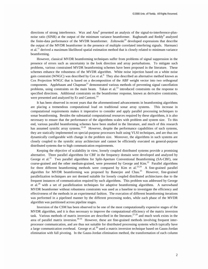
Fig. 1, taken from George et al.26, shows the structure of a basic narrowband adaptive beamformer with a signal arriving from angle θ. Assuming that the data obtained at the n sensors has been transformed into the frequency-domain, resulting in frequency-domain data inputs xo, …, xn-1, the scalar output y for a particular look direction can be expressed as

xw*=y (2.1)

where the * denotes complex-conjugate transposition, and x and w represent the column vector of frequency-domain sensor data and the column vector of adaptive weights wi, respectively. The adaptive property of the weights in the figure is denoted by intersecting arrows.

Fig. 1. Narrowband ABF structure.26

To enable better understanding of MVDR, it is useful to review the basic principles of CBF. In CBF, a delay and sum technique is used for steering in a given look direction. The array is steered by delaying the incoming data with the help of a steering vector, s, and then performing a summation of the delayed outputs, thereby yielding the beamformer output. The steering vector is independent of the incoming data, and may be calculated a priori and stored in memory. The equation for s is given by

Tkdnjkdjjkd eee ],,,,1[)( )sin()1()sin(2)sin( θθθθ −−−−= �s (2.2)

where k is the aforementioned wave number, n is the number of sensor nodes, and d is the distance between the nodes in the array. The reader is referred to Clarkson27 for a more exhaustive theoretical description of CBF.

The CSM, R, is the autocorrelation of the frequency-domain sensor data vector, as given by

}{ *xx ⋅= ER (2.3)

where E is the expectation operation.

The output power for each steering direction is defined as the expected value of the squared magnitude of the beamformer output, as given by

wwwxxw REyEP ***2 }{}|{| =⋅== (2.4)

It may be noted that in CBF, the weight vector w is equal to (s/n), the normalized steering vector, whereas in ABF, the weight vector is computed on the basis of certain data-dependent criteria known as constraints. MVDR is categorized as an adaptive beamformer with linear constraint, the constraint being

g=sw* (2.5)

By imposing this constraint it is ensured that signals from the steering direction of interest are passed with gain g (which equals unity in the case of MVDR), while the output power contributed by interfering signals

xw∗=yΣ

w0

wn-1

x0

xn-1

.

.

.

.

.

.

Node 0

Node n-1

θ xw∗=yΣ

w0

wn-1

x0

xn-1

.

.

.

.

.

.

Node 0

Node n-1

θθ


5

from other directions are minimized using a minimization criterion. Therefore, assuming that s is normalized (i.e. s*s = n), we obtain the weight vector by solving

) ( www

RPMin ∗= constrained to w*s = 1 (2.6)

Solving the above equations by the method of Lagrange multipliers, the weight vector in Eq. (2.6) is obtained as

ss

sw

1*

1

−

−=

R

R (2.7)

By substituting Eq. (2.7) into Eq. (2.6), the scalar output power for a single steering direction is found to be

ss 1*

1)( −=

RP θ (2.8)

The MVDR algorithm calculates the optimal set of weights based on the sampled data, resulting in a beampattern that suppresses the response to directions in which strong sources of interference are present.

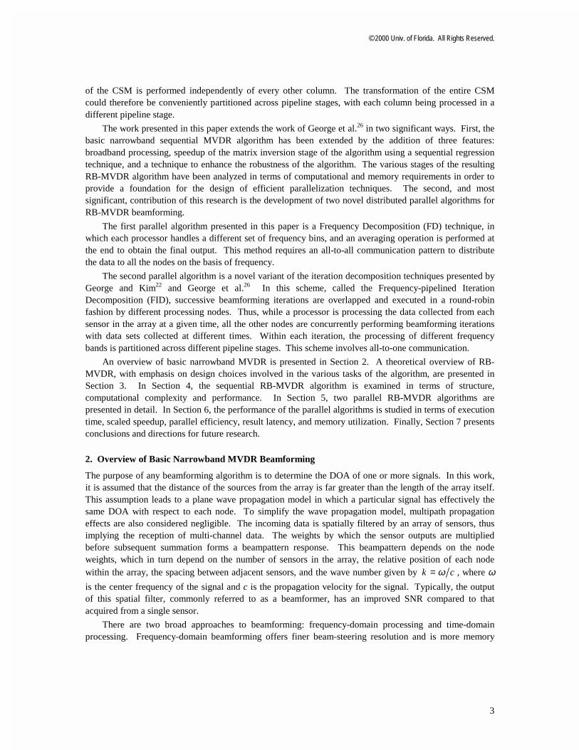
The block diagram of the narrowband sequential MVDR algorithm from George et al.26 is given in Fig. 2 in order to provide a reference point for the enhanced sequential algorithm studied in this research.

Fig. 2. Block diagram of the sequential narrowband MVDR algorithm26.

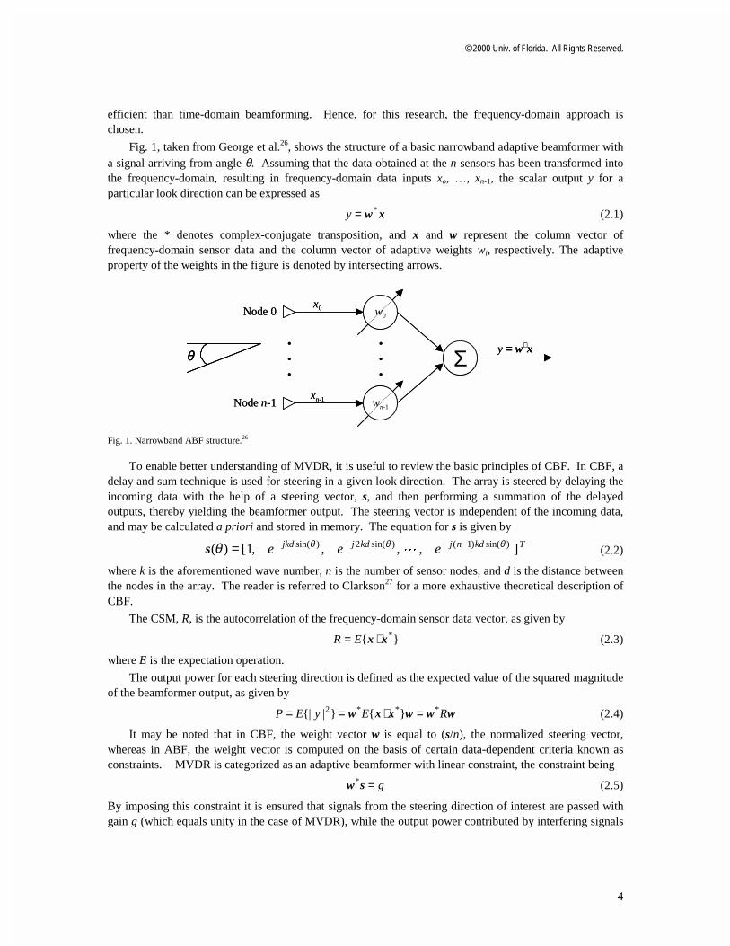
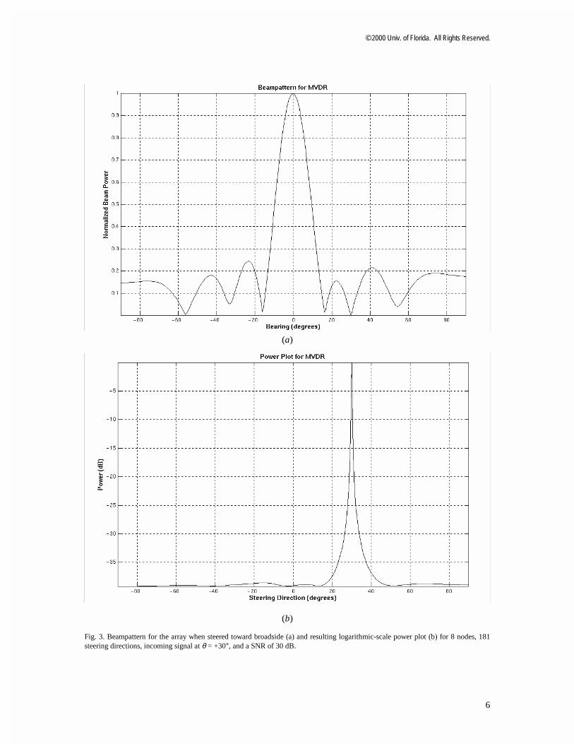
To provide a glimpse into the DOA estimation capability of narrowband MVDR, a typical beamforming power plot with a signal at +30o, and the beampattern looking at broadside (θ = 0°), are shown in Fig. 3. The data in this example was created for a signal having a frequency of 100 Hz. The output of each sensor has, along with the incoming signal, a noise component whose amplitude has normal distribution with zero mean and unit variance. The sensor data has an SNR of 30 dB. Isotropic noise is modeled as a large number of statistically independent stochastic signals arriving at the array from all directions.

In Fig. 3(a), there is a main lobe at broadside (which is the steering direction in this case), and a null at θ = 30° that suppresses the effect of the interference in that direction, leading to an enhanced output plot in Fig. 3(b) that exhibits very little leakage from directions other than the required DOA.

inpu

t sam

ples

R R P

Create

CSM

Compute Inverse Matrix R

Steering R - 1

Steering Vectors

P ( θ )

Create Compute Inverse Matrix

Steering 1

Steering Vectors

( θ )


6

(a)

(b)

Fig. 3. Beampattern for the array when steered toward broadside (a) and resulting logarithmic-scale power plot (b) for 8 nodes, 181 steering directions, incoming signal at θ = +30°, and a SNR of 30 dB.


7

3. The Robust Broadband MVDR Algorithm

The basic narrowband MVDR algorithm described in the previous section provides a foundation on which to incorporate more advanced features that would make the beamformer more accurate, robust, and computationally efficient. Keeping these objectives in mind, a robust broadband MVDR algorithm is implemented and analyzed in order to provide a sequential baseline algorithm for subsequent parallelization. The RB-MVDR algorithm includes three major extensions to the basic algorithm: broadband processing, accelerated matrix inversion, and improved robustness.

3.1. Broadband Processing

Broadband processing involves calculation of the beamformer output for multiple frequency bins, as opposed to narrowband MVDR where only one frequency bin is processed. After the power output has been obtained for each frequency bin, these individual outputs are averaged to yield the final beamformer output. An obvious implication of broadband processing is that there is now a significant FFT computation stage, since the incoming time-domain data needs to be transformed into the frequency domain and the appropriate number of frequency bins, B, is selected from the output of the FFT operation. Moreover, broadband MVDR processing vastly increases the computational requirements of the CSM creation, inversion and steering tasks, since these tasks have to be performed for all the frequency bins under consideration.

The broadband MVDR output is given by

∑==

B

kkav fP

BP

1),(

1)( θθ (3.1)

where fk represents the kth frequency bin and P(fk,θ) is the narrowband output power for that frequency bin.

The main advantage of broadband beamforming is that it avoids inaccuracy of beamformer output due to variation in signal amplitude over multiple frequencies, especially when the SNR is low.

3.2. Speedup of Matrix Inversion using Sequential Regression

CSM inversion is one of the most computationally intensive tasks in the basic MVDR algorithm. The choice of a suitable matrix inversion technique not only affects the sequential execution time of the beamforming algorithm, but also determines the applicability of different parallelization techniques. Matrix inversion is a widely researched area, with numerous matrix inversion methods being used in the literature. Traditionally, most MVDR implementations have used conventional inversion techniques such as Gauss-Jordan Elimination (GJE) and LU Decomposition (LUD). For example, George et al.26 made use of the GJE method with full pivoting, the choice being primarily dictated by the numerical stability of the full pivoting approach and the computationally deterministic nature of the GJE algorithm.

One of the ancillary goals of this research is to arrive at a computationally efficient matrix inversion technique for broadband MVDR beamforming. To this end, GJE and LUD are compared in terms of execution time and memory utilization with another technique known as sequential regression (SER).

Gauss-Jordan Elimination is used to solve the equation

IXR =⋅ (3.2)

where R is the square matrix (in this case, the CSM) whose inverse is to be determined, X is the unknown inverse CSM, and I is the identity matrix. Elementary row transformation operations are applied to R to reduce it to I, and the same operations are also performed on the identity matrix I. When R has been completely reduced to I, the right-hand side of the equation contains R−1, obtained via the row transformations performed on I. In the comparative analysis presented in this section, GJE with full


8

pivoting is used, in which rows as well as columns are interchanged in such a way as to place a particularly desirable element in the diagonal position where it can be used as a pivot for subsequent transformations.28 Interestingly, in this method it is not necessary to maintain a separate storage area in memory for the identity matrix. The inverse matrix is built up in the original matrix as the original matrix is destroyed, and the result is obtained in-place. To offset the effect of the column interchanges, an unscrambling operation is performed on the solution obtained as a result of the transformations.

The two main innermost loops of the GJE algorithm, each containing one subtraction and one multiplication, are each executed n3 times. This configuration yields a floating-point operations count of 2n3 and a computational complexity of O(n3).

The second method of CSM inversion considered here is LU Decomposition. In this method, a matrix R is decomposed as a product of two matrices L and U, where L is a lower triangular matrix and U is an upper triangular matrix.28 Thus,

RUL =⋅ (3.3)

This decomposition is used to obtain the solution of

IXULXULXR =⋅⋅=⋅⋅=⋅ )()( (3.4)

First, a matrix Y is obtained which satisfies the equation

IYL =⋅ (3.5)

This solution is accomplished by the method of forward substitution, in which each element yjk of the matrix Y is obtained by the equation

jj

j

mmkjmjk

jk l

yliy

∑−=

−

=

1

1)(

(3.6)

and then X is obtained by solving the equation

YXU =⋅ (3.7)

The solution of Eq. 3.7 is obtained using the method of back substitution, in which each element xjk of the matrix X is obtained by the equation

jj

n

jmmkjmjk

jk u

xuy

x∑−

= += 1)(

(3.8)

Partial pivoting is used in this implementation of LUD. This choice is guided by two observations in the literature: firstly, it has been observed that full pivoting cannot be implemented efficiently, and secondly, partial pivoting is sufficient to ensure numerical stability in LUD.28 Both the forward substitution and back substitution tasks contain an inner loop comprising of one floating-point multiplication and one floating-point subtraction (i.e. 2 floating-point operations). After eliminating redundant computations on zero elements, such as the leading zeroes present in the identity matrix, forward substitution and back substitution require n3/6 and n3/2 executions of the inner loop, respectively. Thus, the two tasks require n3/3 and n3 operations, respectively. Similarly, decomposition of the matrix into its triangular factors requires 2n3/3 operations. Hence, the total operations count is 2n3, just as in the case of GJE.28 The overall computational complexity is therefore O(n3).

The computational complexity of the CSM inversion task can be reduced by using SER. This technique has traditionally been used in adaptive signal processing algorithms such as Recursive Least Squares (RLS), and is now gaining wide acceptance in the field of adaptive beamforming. SER is an


9

iterative method in which the inverse CSM is updated at each iteration and not obtained via explicit inversion of the CSM. This method is based on the well-known matrix inversion lemma27, 29 given by

1111111 )()( −−−−−−− +−=+ DACBDABAABCDA (3.9)

where A is a matrix of size (n × n), B and D are vectors of size (n × 1) and (1 × n) respectively, and C is a scalar.

The inverse CSM update equation is obtained from the CSM update equation. In this work, the CSM estimate is updated with new incoming data using exponential averaging at every iteration, as given by the CSM update equation

Hiiii RR 111 )1(ˆˆ+++ −+= xxαα (3.10)

where α is the forgetting factor, which determines the weight given to the previous CSM estimate relative

to the new frequency domain data vector, and iR̂ is an estimate of the CSM for iteration i.

In the SER technique, the inverse CSM is initialized with a non-zero value (1/0)I, where 0 is a small constant and I is the (n × n) identity matrix. The purpose of this initialization is to prevent the matrix from becoming singular. At every subsequent iteration, the inverse CSM is updated with the new frequency-domain data using the matrix inversion lemma.

Therefore, setting A = α iR̂ , B = 1+ix , C = (1−α), and D = Hi 1+x , we get

−+

−−=

+−

+

−++

−−−

+1

11

111

111

1 ˆ)1(

ˆˆ1ˆ1ˆ

iiHi

iHiii

iiR

RRRR

xx

xx

αααα

α (3.11)

By applying the Hermitian property of the CSM, the complexity of the SER algorithm is reduced to O(n2), as opposed to the complexity of the GJE and LUD techniques which was O(n3).

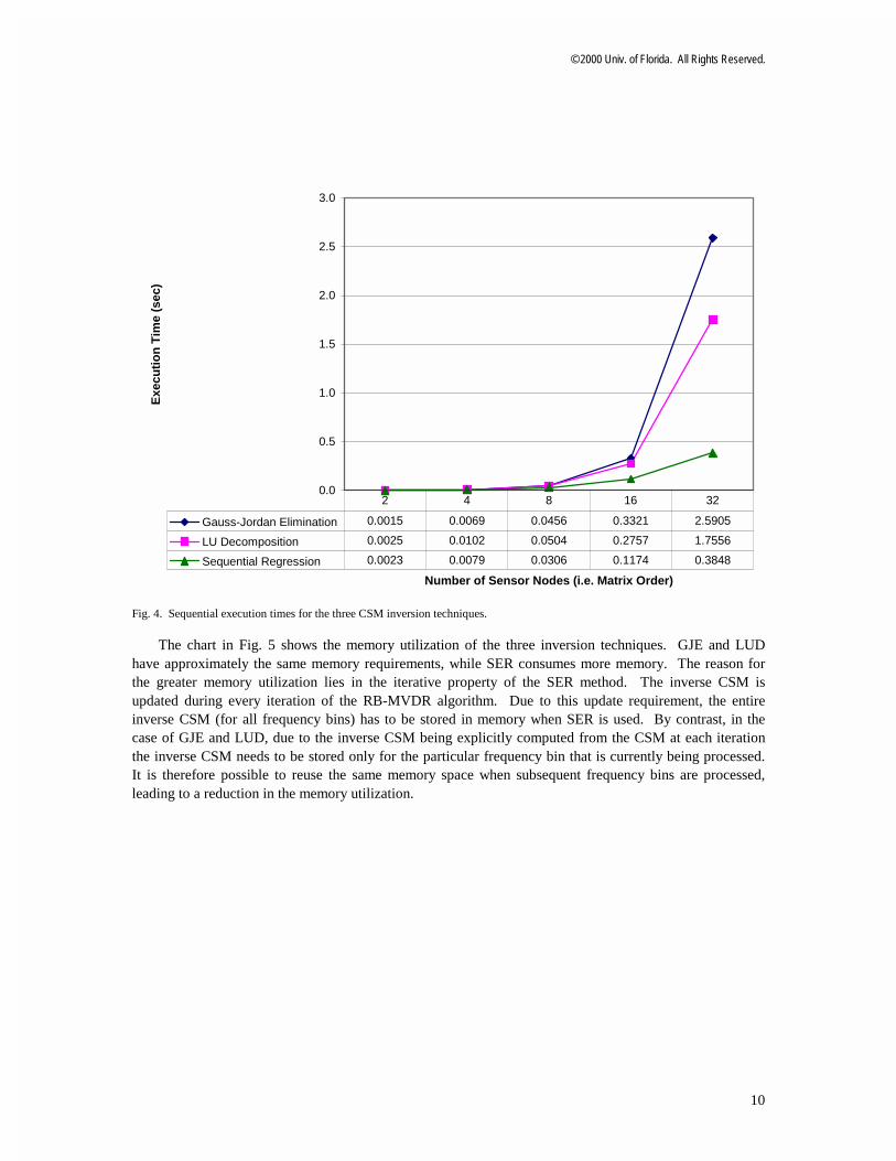
To ascertain the relative merits of the three methods in order to select the best CSM inversion method for the RB-MVDR algorithm, an experimental analysis of the three aforementioned methods was performed. The three CSM inversion techniques were implemented in C code for 192 frequency bins. The platform used for this comparative performance analysis was a Linux PC with a 400MHz Intel Celeron processor, 128KB of L2 cache and 64MB of RAM. This platform was selected for convenience, since the performance capabilities of some embedded, floating-point, DSP systems (e.g. the SHARC from Analog Devices) with hand-optimized beamforming code were found to be roughly comparable to those of a Celeron PC. The sequential execution times measured for the three matrix inversion methods are shown in Fig. 4. It is seen that SER becomes significantly faster than the other two methods as the number of nodes is increased.


10

0.0

0.5

1.0

1.5

2.0

2.5

3.0

Number of Sensor Nodes (i.e. Matrix Order)

Exe

cuti

on

Tim

e (s

ec)

Gauss-Jordan Elimination 0.0015 0.0069 0.0456 0.3321 2.5905

LU Decomposition 0.0025 0.0102 0.0504 0.2757 1.7556

Sequential Regression 0.0023 0.0079 0.0306 0.1174 0.3848

2 4 8 16 32

Fig. 4. Sequential execution times for the three CSM inversion techniques.

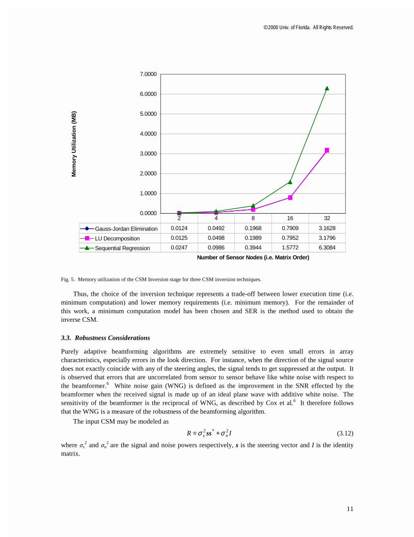
The chart in Fig. 5 shows the memory utilization of the three inversion techniques. GJE and LUD have approximately the same memory requirements, while SER consumes more memory. The reason for the greater memory utilization lies in the iterative property of the SER method. The inverse CSM is updated during every iteration of the RB-MVDR algorithm. Due to this update requirement, the entire inverse CSM (for all frequency bins) has to be stored in memory when SER is used. By contrast, in the case of GJE and LUD, due to the inverse CSM being explicitly computed from the CSM at each iteration the inverse CSM needs to be stored only for the particular frequency bin that is currently being processed. It is therefore possible to reuse the same memory space when subsequent frequency bins are processed, leading to a reduction in the memory utilization.


11

0.0000

1.0000

2.0000

3.0000

4.0000

5.0000

6.0000

7.0000

Number of Sensor Nodes (i.e. Matrix Order)

Mem

ory

Uti

lizat

ion

(M

B)

Gauss-Jordan Elimination 0.0124 0.0492 0.1968 0.7909 3.1628

LU Decomposition 0.0125 0.0498 0.1989 0.7952 3.1796

Sequential Regression 0.0247 0.0986 0.3944 1.5772 6.3084

2 4 8 16 32

Fig. 5. Memory utilization of the CSM Inversion stage for three CSM inversion techniques.

Thus, the choice of the inversion technique represents a trade-off between lower execution time (i.e. minimum computation) and lower memory requirements (i.e. minimum memory). For the remainder of this work, a minimum computation model has been chosen and SER is the method used to obtain the inverse CSM.

3.3. Robustness Considerations

Purely adaptive beamforming algorithms are extremely sensitive to even small errors in array characteristics, especially errors in the look direction. For instance, when the direction of the signal source does not exactly coincide with any of the steering angles, the signal tends to get suppressed at the output. It is observed that errors that are uncorrelated from sensor to sensor behave like white noise with respect to the beamformer.6 White noise gain (WNG) is defined as the improvement in the SNR effected by the beamformer when the received signal is made up of an ideal plane wave with additive white noise. The sensitivity of the beamformer is the reciprocal of WNG, as described by Cox et al.6 It therefore follows that the WNG is a measure of the robustness of the beamforming algorithm.

The input CSM may be modeled as

IR ns2*2 σσ += ss (3.12)

where 1s2 and 1n

2 are the signal and noise powers respectively, s is the steering vector and I is the identity matrix.


12

The input SNR is

2

2

n

sinSNR

σσ

= (3.13)

Similarly, the output may be written as *2**2* wwwsswww nsR σσ += (3.14)

The output SNR is given by

*2

2*2 ||

ww

sw

n

soutSNR

σσ

= (3.15)

Therefore, the WNG is

wwww

sw**

2* 1|| ===in

out

SNR

SNRWNG (3.16)

where |w*s|2 = 1 because of the MVDR unity response constraint. In the case of CBF, WNG = n, the number of sensor nodes.

There are various prevalent methods to make the MVDR algorithm more robust. Two popular robustness enhancement techniques are considered in an effort to arrive at the method most suitable for the RB-MVDR algorithm.

In the first method, a small amount of constant noise 0 is injected into the diagonal elements of R before inversion. The weight vector is therefore calculated using (R + εI) instead of R. When 0 = 0, the beamformer is identical to purely adaptive MVDR, while large values of 0 make it identical to CBF. Thus, by using values of 0 between zero and infinity, we make the MVDR beamformer less sensitive to look direction errors, thereby preventing signal suppression.

The second method is a variant of WNGC known as Cox Projection WNGC.6 In this technique, instead of adding noise to the diagonal elements of the CSM, the WNGC is applied by first calculating the purely adaptive MVDR weight vector and then adjusting it to satisfy a white noise gain constraint. The Cox Projection WNGC procedure is briefly outlined as follows:

(a) First, the purely adaptive MVDR weight wMVDR is calculated using Eq. 2.7.

(b) Then, each weight is decomposed into two parts:

(i) w1, which is parallel to the steering vector, s, and equal to the CBF weight vector, wCBF.

(ii) w2, which is perpendicular (orthogonal) to s.

(c) Since w2 is orthogonal to s, we have w2Hs = 0 = sHw2, and thus, w2 can be scaled by a weighting

factor b without violating the MVDR constraint.

Therefore, the modified weight vector is

2CBFnew www ×+= b (3.17)

The factor b = 0 in the case of CBF and b = 1 in the case of purely adaptive MVDR.

Cox Projection WNGC is the technique selected for this research. The advantage of using this particular method in the RB-MVDR algorithm is that the Cox Projection technique is independent of the CSM creation and inversion stages. Any inversion method can be chosen without affecting the robustness enhancement strategy, since the application of WNGC in the Cox Projection method is done in the steering stage. This issue is of special importance because the SER method of obtaining the inverse CSM has been chosen for this work, and an iterative method such as SER would require a significant amount of modification if the WNGC is applied in the CSM creation stage.


13

Values of b approaching 1 produce sharper peaks in the beamformer output and enable more accurate DOA estimation. This characteristic indicates proximity to the purely adaptive MVDR case. By contrast, when b = 0, the beamformer has relatively inferior detection capabilities and is identical to the CBF case.

When the signal source has a DOA that does not coincide with any of the steering angles considered, the output in the signal direction is suppressed or attenuated for values of b close to 1. This phenomenon is a result of the highly adaptive and thus error-sensitive nature of the pure MVDR algorithm. By contrast, decreasing the value of b increases the amount of robustness in the beamformer. The choice of the weighting factor represents a tradeoff between selectivity and robustness.

4. Sequential RB-MVDR Algorithm and Performance

This section presents an analysis of the different computational tasks of the sequential RB-MVDR algorithm, and evaluates the performance of each stage of the algorithm in terms of execution time.

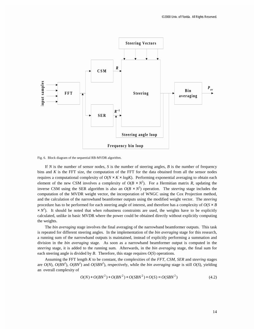
4.1. Sequential RB-MVDR tasks

The principal stages in the sequential RB-MVDR algorithm are FFT, CSM, SER, steering and bin averaging. Fig. 6 shows a block diagram for the various computational stages in the sequential RB-MVDR algorithm. The incoming time-domain sensor data is transformed into frequency-domain data in the FFT stage. The appropriate set of frequency bins is selected from the FFT output, and the CSM and inverse CSM are calculated from this subset of the FFT output. The CSM and SER stages are depicted as independent blocks, since the inverse CSM is updated directly from the output of the FFT stage rather than involving explicit inversion of the CSM. The steering stage consists of the operations of calculating the MVDR weight vector, manipulating it to apply the WNGC, and the final calculation of the output powers. The application of a robustness constraint requires explicit computation of the MVDR weight vector using Eq. 2.7, because the MVDR weights need to be subsequently adjusted to satisfy the WNGC. Applying the weight vector thus obtained, the narrowband output for each frequency bin, fk, is calculated as

newHnew ww RfP k =),( θ (4.1)

It is observed that the CSM, SER and steering stages are repeated for each frequency bin of interest. Moreover, the processing of every frequency bin is independent of every other frequency bin. When the power outputs have been obtained for all the frequency bins, these narrowband outputs are averaged in the bin averaging stage to obtain the final broadband output for each steering angle.


14

F F T

C S M

S E R

Steer ing

Steer ing Vectors

B i na v e r a g i n g

i npu

t sa

mpl

es

F requency b in loop

Steer ing angle loop

P a v

R−1

R

Fig. 6. Block diagram of the sequential RB-MVDR algorithm.

If N is the number of sensor nodes, S is the number of steering angles, B is the number of frequency bins and K is the FFT size, the computation of the FFT for the data obtained from all the sensor nodes requires a computational complexity of O(N × K × logK). Performing exponential averaging to obtain each element of the new CSM involves a complexity of O(B × N2). For a Hermitian matrix R, updating the inverse CSM using the SER algorithm is also an O(B × N2) operation. The steering stage includes the computation of the MVDR weight vector, the incorporation of WNGC using the Cox Projection method, and the calculation of the narrowband beamformer outputs using the modified weight vector. The steering procedure has to be performed for each steering angle of interest, and therefore has a complexity of O(S × B × N2). It should be noted that when robustness constraints are used, the weights have to be explicitly calculated, unlike in basic MVDR where the power could be obtained directly without explicitly computing the weights.

The bin averaging stage involves the final averaging of the narrowband beamformer outputs. This task is repeated for different steering angles. In the implementation of the bin averaging stage for this research, a running sum of the narrowband outputs is maintained, instead of explicitly performing a summation and division in the bin averaging stage. As soon as a narrowband beamformer output is computed in the steering stage, it is added to the running sum. Afterwards, in the bin averaging stage, the final sum for each steering angle is divided by B. Therefore, this stage requires O(S) operations.

Assuming the FFT length K to be constant, the complexities of the FFT, CSM, SER and steering stages are O(N), O(BN2), O(BN2) and O(SBN2), respectively, while the bin averaging stage is still O(S), yielding an overall complexity of

)()()()()()( 2222 SBNOSOSBNOBNOBNONO =++++ (4.2)


15

4.2. Sequential RB-MVDR performance

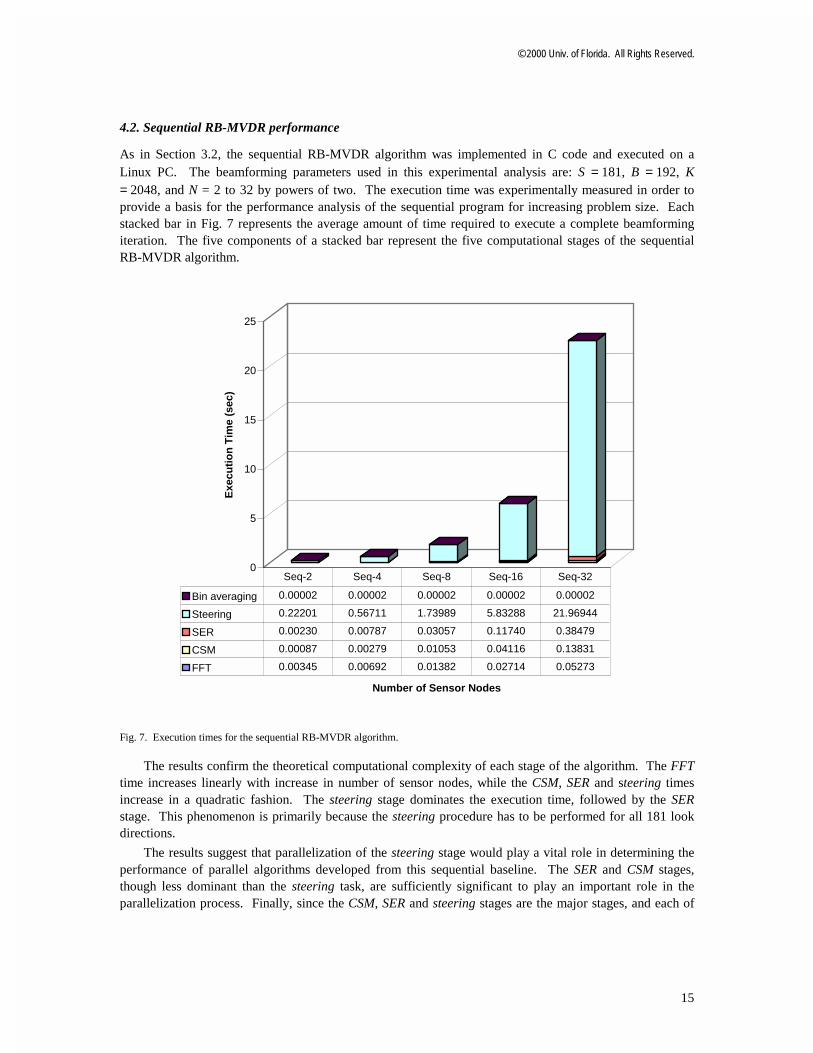
As in Section 3.2, the sequential RB-MVDR algorithm was implemented in C code and executed on a Linux PC. The beamforming parameters used in this experimental analysis are: S = 181, B = 192, K = 2048, and N = 2 to 32 by powers of two. The execution time was experimentally measured in order to provide a basis for the performance analysis of the sequential program for increasing problem size. Each stacked bar in Fig. 7 represents the average amount of time required to execute a complete beamforming iteration. The five components of a stacked bar represent the five computational stages of the sequential RB-MVDR algorithm.

0

5

10

15

20

25

Exe

cuti

on

Tim

e (s

ec)

Number of Sensor Nodes

Bin averaging 0.00002 0.00002 0.00002 0.00002 0.00002

Steering 0.22201 0.56711 1.73989 5.83288 21.96944

SER 0.00230 0.00787 0.03057 0.11740 0.38479

CSM 0.00087 0.00279 0.01053 0.04116 0.13831

FFT 0.00345 0.00692 0.01382 0.02714 0.05273

Seq-2 Seq-4 Seq-8 Seq-16 Seq-32

Fig. 7. Execution times for the sequential RB-MVDR algorithm.

The results confirm the theoretical computational complexity of each stage of the algorithm. The FFT time increases linearly with increase in number of sensor nodes, while the CSM, SER and steering times increase in a quadratic fashion. The steering stage dominates the execution time, followed by the SER stage. This phenomenon is primarily because the steering procedure has to be performed for all 181 look directions.

The results suggest that parallelization of the steering stage would play a vital role in determining the performance of parallel algorithms developed from this sequential baseline. The SER and CSM stages, though less dominant than the steering task, are sufficiently significant to play an important role in the parallelization process. Finally, since the CSM, SER and steering stages are the major stages, and each of


16

these tasks is performed independently for every frequency bin, the frequency domain should be a convenient and effective basis for decomposition techniques.

5. Parallel Algorithms for RB-MVDR Beamforming

Beamforming with a large number of sensors and over a wide range of frequencies and steering angles presents computational requirements that may not be efficiently met by conventional processor performance, thereby necessitating the application of parallel processing to cope with complex beamforming algorithms like RB-MVDR. In the distributed system model used here, each sensor is associated with a smart node with its own processor and memory, and the nodes are connected by a communication network. Parallel algorithms seek to exploit the various sources of parallelism that are inherent in sequential beamforming algorithms like RB-MVDR. The granularity of a parallel algorithm is defined as the level at which the sequential algorithm is partitioned between processing nodes, and is dictated by the ratio of computation to interprocessor communication in the algorithm. In a coarse-grained decomposition, communication occurs less frequently, between large sections of computation. Fine-grained decomposition techniques require more communication, as partitioning is done at the level of small computational segments. A medium-grained decomposition is intermediate in its properties.

The application of parallel processing to distributed systems such as a sonar array makes it imperative for designers of parallel beamforming algorithms to minimize the amount of interprocessor communication that would be necessary in the algorithm. Thus, fine-grained parallel algorithms are not deemed suitable for such systems due to the higher communication overhead present in typical distributed systems. By contrast, the lower amount of communication required by coarse- and medium-grained decompositions render them more effective for beamforming applications.

There are various candidate approaches towards parallelization of beamforming algorithms. Some of the methods developed and analyzed in the literature on parallel beamforming algorithms are:

(a) Iteration Decomposition: Iteration decomposition is a coarse-grained decomposition technique. In this method, successive independent beamforming iterations are allocated to different processing nodes and executed in a pipelined fashion, thus taking complete advantage of the lack of loop-carried dependencies. To take the example of a 3-node array, node 0 would be assigned iterations 0, 3, 6, 9, etc., node 1 would be assigned iterations 1, 4, 7, 10, etc., and so on. This method is explained and analyzed in the literature.21-24 George et al.26 presented a variant of this coarse-grained algorithm that contains a computation component and a communication component. In the computation component, consecutive beamforming iterations are scheduled in a round-robin manner over the nodes of the array, and their execution is pipelined. The communication component of the algorithm helps to greatly reduce communication overhead by spooling multiple data samples into a single packet. Moreover, communication latency is hidden through concurrent execution of computation and communication, made possible with multithreading.

(b) Angle Decomposition: An alternative approach to parallelization that has been described in the literature21-24 is angle decomposition. As opposed to iteration decomposition, this technique is a classic example of a medium-grained approach to parallelization. Each node is allotted the task of calculating the output power for a subset of the steering angles of interest. In a 4-node array, for instance, if the output is needed for 180 steering angles, each node would perform the steering for 45 of those angles. This method requires a relatively greater amount of communication, since the entire input data must be distributed to all the processors.

However, neither of these methods is devoid of disadvantages, especially when applied to complex adaptive beamforming algorithms such as RB-MVDR. Iteration decomposition often suffers from asymmetrical partitioning of computational load between the pipeline stages of a single beamforming cycle, as well as the difficulty inherent in determining partitioning schemes for each individual sub-task such as CSM, SER, and steering. Angle decomposition is unsuitable for the RB-MVDR algorithm


17

primarily because it parallelizes only the steering stage while failing to exploit sources of parallelism in the other stages, and because of the tremendous stress placed on the communication network by the all-to-all transmission of the entire data set between the nodes. To overcome the disadvantages of the aforementioned techniques and to enable more efficient parallelization, two methods of parallelization are presented: Frequency Decomposition (FD) and Frequency-pipelined Iteration Decomposition (FID).

5.1 Frequency Decomposition (FD) method

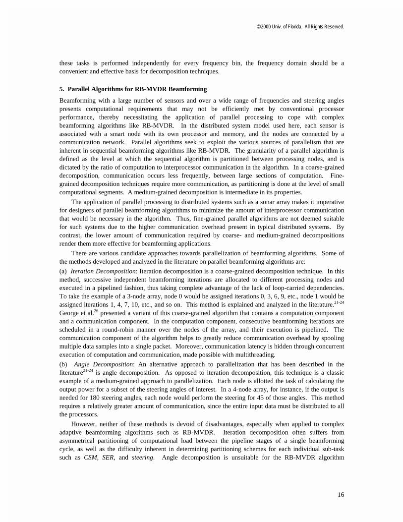
The frequency decomposition technique may be termed a coarse-grained method of parallelization due to the reduction in the frequency of communication with data packing. A study of the structure and dependencies inherent in the sequential RB-MVDR algorithm makes it apparent that every major computational task in the algorithm can be performed for each frequency bin independent of other frequency bins. It is this lack of dependencies between the narrowband components that the FD algorithm exploits. Each processor is assigned the responsibility for processing a different subset of frequency bins (i.e. a different frequency band). After each node has executed an FFT on the data that has been obtained by its sensor, it distributes the data to the other nodes on the basis of frequency. Thus, the first node gets the data corresponding to the first set of frequencies, the second node gets the data corresponding to the second set of frequencies, and so on. At the end of each iteration, the outputs computed by each node for the frequency bins allocated to it are sent to one of the nodes. This node averages the individual narrowband outputs to obtain the final power output. The responsibility for this bin averaging task is alternated in a round-robin fashion between the nodes. The FD algorithm is illustrated in Fig. 8 for a 3-node case.

CSM SER Steering

CSM SER Steering

all-

to-a

ll co

mm

unic

atio

n

FFT

FFT

FFT

CSM SER Steering

CSM SER Steering

all-

to-a

ll co

mm

unic

atio

n

FFT

FFT

FFT

No

de

0N

od

e 1

No

de

2

Result Latency

process iteration i−1 process iteration i process iteration i+1

proc

ess

1/3

of f

requ

ency

bin

spr

oces

s1/

3 of

fre

quen

cy b

ins

proc

ess

1/3

of f

requ

ency

bin

s

Bin avg.(from

previousiteration)

CSM SER Steering

CSM SER Steering

CSM SER Steering

FFT

FFT

FFT

Bin avg.(from

previousiteration)

CSM SER Steering

Bin avg.(from

previousiteration)

CSM SER Steering

all-

to-a

ll co

mm

unic

atio

n

Fig. 8. Block diagram of FD in a 3-node configuration.

In Fig. 8, i refers to the iteration number. The horizontal arrows signify the flow of information within the same node, while vertical intersections between these lines represent the flow of information between different nodes (i.e. interprocessor communication). The horizontal ordering of various


18

computational blocks represent the temporal sequence of different computational stages of the parallel algorithm. Different iterations are denoted by the shaded background rectangles, while each node processes a subset of the frequency bins.

It is apparent from the preceding discussion that this method requires an all-to-all communication pattern for the initial distribution of data and an all-to-one communication pattern for the final accumulation of individual outputs. The overhead of initiating communication is therefore incurred twice, causing a significant increase in communication time. This overhead is reduced by a data packing technique, wherein the two instances of communication performed by each node are combined into one packet, thereby incurring the communication overhead only once rather than twice. In this technique, the narrowband outputs of a particular beamforming iteration are concatenated with the frequency domain data of the next iteration. Since a single node is responsible for performing the bin averaging task for a particular iteration, only that node receives the concatenated packet, while all the other nodes merely receive the frequency domain data that is to be processed in that iteration. The total amount of data communicated is unchanged by this scheme, since the data packing strategy merely reduces the overhead of initiating communication twice.

The result latency of an algorithm is defined as the delay between the collection of data and the computation of the final output. The data packing strategy used in FD causes a slight increase in the result latency, as the result is obtained only at the end of the FFT and communication stages of the succeeding iteration.

In this implementation, the bin averaging operation in FD is executed in two phases. At the end of the steering stage, each node calculates the average of the beamformer outputs for the frequency bins assigned to it. Subsequently, each node transmits this partial average to one of the nodes, which then computes the average of the outputs received from all the nodes. The responsibility of collecting the outputs of the individual nodes and computing their average for a particular beamforming iteration is alternated among all the nodes in a round-robin fashion. Bin averaging is the only stage of the algorithm that is not parallelized in FD. However, the fact that each node maintains a running sum of the outputs for its assigned frequency bins renders this task nearly trivial.

Assuming the FFT length to be constant, the complexities of the FFT, CSM, SER and steering stages after parallelization are O(1), O(BN), O(BN) and O(SBN), respectively, whereas the bin averaging stage is still O(S). The overall parallel complexity is thus

)()()()()()1( SBNOSOSBNOBNOBNOO =++++ (5.1)

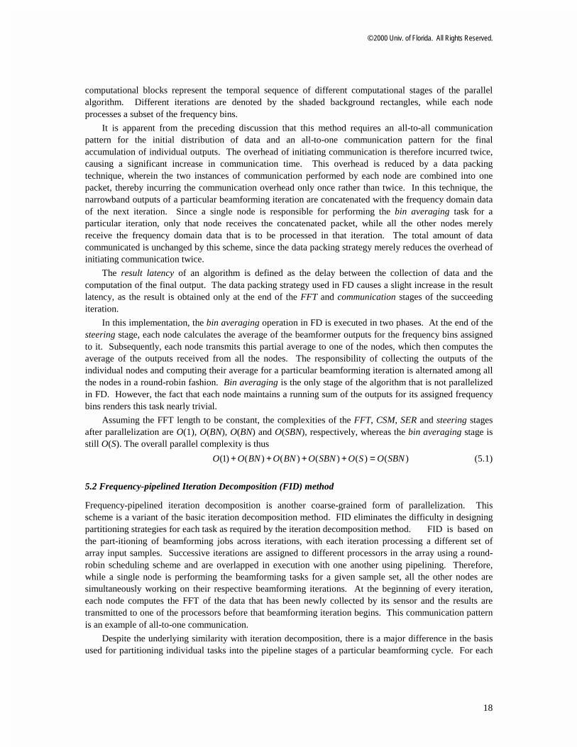
5.2 Frequency-pipelined Iteration Decomposition (FID) method

Frequency-pipelined iteration decomposition is another coarse-grained form of parallelization. This scheme is a variant of the basic iteration decomposition method. FID eliminates the difficulty in designing partitioning strategies for each task as required by the iteration decomposition method. FID is based on the part-itioning of beamforming jobs across iterations, with each iteration processing a different set of array input samples. Successive iterations are assigned to different processors in the array using a round-robin scheduling scheme and are overlapped in execution with one another using pipelining. Therefore, while a single node is performing the beamforming tasks for a given sample set, all the other nodes are simultaneously working on their respective beamforming iterations. At the beginning of every iteration, each node computes the FFT of the data that has been newly collected by its sensor and the results are transmitted to one of the processors before that beamforming iteration begins. This communication pattern is an example of all-to-one communication.

Despite the underlying similarity with iteration decomposition, there is a major difference in the basis used for partitioning individual tasks into the pipeline stages of a particular beamforming cycle. For each


19

node, the processing of different subsets of the frequency bins of interest is partitioned across the n pipeline stages in a beamforming iteration. The first subset of frequency bins (set 0) is processed in the first pipeline stage, the second subset of frequency bins (set 1) in the second pipeline stage, and so on.

Fig. 9 shows the block diagram of the FID algorithm for a 3-node case. The conventions are similar to Fig. 8. As seen from the figure, the CSM, SER and steering operations in the different pipeline stages of a single beamforming cycle do not have any dependencies across pipeline stages.

i terat ion i

C S M S E R Steer ingBinavg.

No

de

0N

od

e 1

No

de

2

Effective Execution Time

Result Latency

FFT

FFT

iter.i+2

i ter.i+2

process1 / 3 of frequency bins


proc

ess

itera

tions

proc

ess

itera

tions

proc

ess

itera

tions

FFT

iter.i+2

i terat ion i+1

C S M S E R Steer ing

iterat ion i+2


iterat ion i

C S M S E R Steer ingC S M

iterat ion i

S E R Steer ing

C S M

iterat ion i+1

S E R Steer ing

C S M

iterat ion i−1

S E R Steer ingBinavg.

iter.i+1

FFT

FFT

iter.i+1

FFT

iter.i+1

C S M S E R Steer ingBinavg.

i terat ion i−2

FFT

iter.i

FFT

iter.i

FFT

iter.i


iterat ion i−1


all-

to-o

ne c

omm

unic

atio

n

all-

to-o

ne c

omm

unic

atio

n

all-

to-o

ne c

omm

unic

atio

n

Fig. 9. Block diagram of FID in a 3-node configuration.

The result latency of FID is higher than that of the sequential algorithm, because the result is obtained only at the end of the entire beamforming cycle, which includes communication and pipeline overheads.

Like FD, FID parallelizes all the stages of the sequential algorithm except for the bin averaging stage. Again, if the FFT length K is assumed to be constant, the complexity of the FFT, CSM, SER and steering stages are O(1), O(BN), O(BN) and O(SBN), respectively, while the bin averaging stage has a complexity of O(S) as before. Therefore, the overall parallel complexity is

)()()()()()1( SBNOSOSBNOBNOBNOO =++++ (5.2)

Table 1 compares the computational complexities of the sequential algorithm and the two parallel algorithms. With the use of a linear configuration of distributed processors, the parallel algorithm complexities are reduced by a factor of N as compared to the sequential algorithm.


20

Table 1. Computational complexities of the sequential and parallel RB-MVDR algorithms.

ALGORITHM COMPLEXITY SEQ O(SBN2) FD O(SBN) FID O(SBN)

6. Performance Analysis of Parallel RB-MVDR Algorithms

To gain insight into the various factors affecting the performance of the parallel algorithms described in the previous section, each algorithm was implemented using C-MPI and executed on a cluster of Linux PCs. Message Passing Interface (MPI) is a standardized library of functions and macros used in C/C++ or Fortran programs for message-passing communication and synchronization.22 In this experimental analysis, the average time spent in communication function calls such as MPI_Send and MPI_Recv is denoted as communication time. The cluster employed included up to 32 PCs as sensor/processor nodes, each having a 400 MHz Intel Celeron processor, 128KB of L2 cache and 64 MB of RAM. The nodes were connected by a switched Fast Ethernet network. The beamforming parameters used were the same as those in Section 4, and thus provide a fair comparison of the parallel algorithms with their sequential baseline.

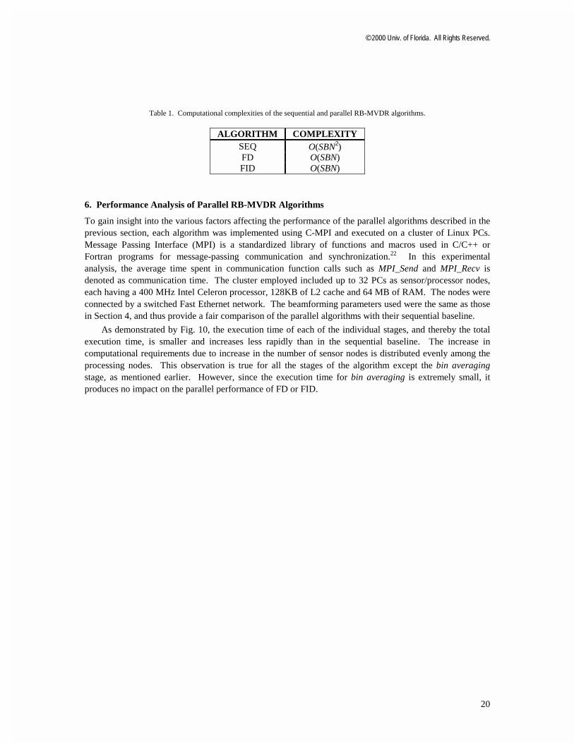
As demonstrated by Fig. 10, the execution time of each of the individual stages, and thereby the total execution time, is smaller and increases less rapidly than in the sequential baseline. The increase in computational requirements due to increase in the number of sensor nodes is distributed evenly among the processing nodes. This observation is true for all the stages of the algorithm except the bin averaging stage, as mentioned earlier. However, since the execution time for bin averaging is extremely small, it produces no impact on the parallel performance of FD or FID.


21

0.0

0.1

0.2

0.3

0.4

0.5

0.6

0.7

0.8

0.9

1.0

Exe

cuti

on

Tim

e (s

ec)

Number of Nodes

Bin averaging 0.00003 0.00002 0.00002 0.00002 0.00002 0.00002 0.00002 0.00002 0.00003 0.00003

Steering 0.11768 0.15210 0.23949 0.41663 0.78173 0.11607 0.15316 0.24062 0.41720 0.78970

SER 0.00122 0.00217 0.00396 0.00798 0.01469 0.00117 0.00206 0.00403 0.00800 0.01516

CSM 0.00050 0.00081 0.00137 0.00288 0.00531 0.00048 0.00077 0.00149 0.00281 0.00559

Communication 0.00258 0.00885 0.01630 0.03797 0.08544 0.00093 0.00158 0.00348 0.00529 0.00720

FFT 0.00182 0.00180 0.00186 0.00186 0.00173 0.00178 0.00185 0.00179 0.00181 0.00179

FD-2 FD-4 FD-8 FD-16 FD-32 FID-2 FID-4 FID-8 FID-16 FID-32

Fig. 10. Average execution time per iteration as a function of system and problem size for the parallel RB-MVDR algorithms with 192 frequency bins, 181 steering angles and 512 iterations on a PC cluster.

The parallel execution times clearly indicate that the steering task is by far the most computationally intensive task even in the parallel algorithms, the primary reason being that the steering stage is O(SBN) whereas the CSM and SER stages have a O(BN) complexity. The CSM and SER tasks only loop over the number of frequency bins and do not depend on the number of steering angles. From the figure, it can be seen that FFT time and bin averaging time are almost constant because they are O(S) operations in the parallel algorithm, while the CSM, SER and steering times increase in a nearly linear fashion. Notably, the CSM, SER and steering times are slightly higher for FID as compared to FD, which is a result of pipeline overhead. Another key observation is that the communication time is much higher in FD than in FID, and also increases more rapidly with system and problem size. This higher communication time is because of the all-to-all nature of the communication in FD, as opposed to the all-to-one communication pattern in FID.

The scaled speedup of any parallel algorithm is defined as the ratio of the sequential execution time to the parallel execution time. This performance metric takes into account the fact that the problem size is also scaled upwards as the number of processing nodes is increased. Parallel efficiency is the ratio of the


22

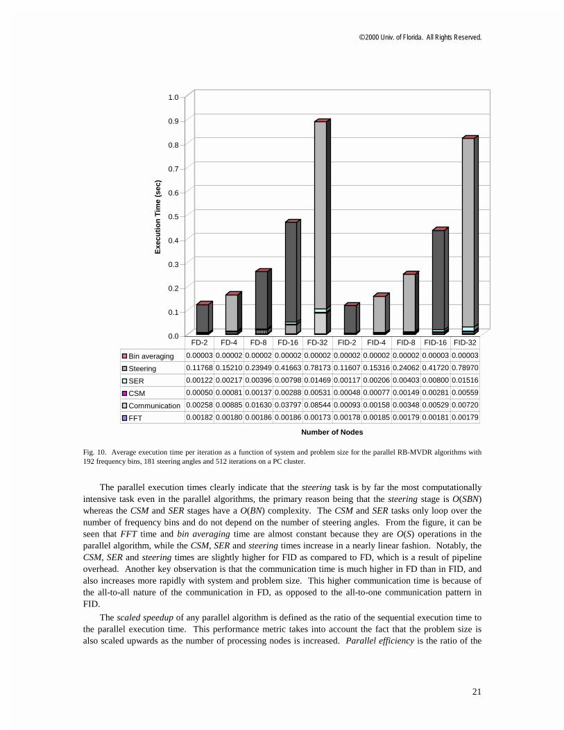
scaled speedup to the ideal speedup, which is equal to the number of processors. Fig. 11 shows the scaled speedup for the two parallel algorithms.

0

5

10

15

20

25

30

2 4 8 16 32

Number of Nodes

Sca

led

Sp

eed

up

FD

FID

Fig. 11. Scaled speedup for FD and FID algorithms as a function of the system and problem size.

From Fig. 11, it can be observed that both parallel algorithms scale effectively with an increase in the system and problem size. However, FID exhibits higher speedup as compared to FD, with a widening gap as the size of the system and problem is increased. The primary reason for the lower speedup demonstrated by FD is the higher communication time for FD as compared to FID. The parallel efficiency results in Fig. 12 further exemplify this trend. The faster decrease in parallel efficiency with system and problem size in the case of FD is due to the relatively faster growth of communication time exhibited by FD. Communication time has a relatively smaller effect on the performance of FID. However, even in the case of FID, the efficiency is less than ideal due to pipeline overhead. In FID, the effect of communication and other overhead becomes less significant compared to the computational savings at higher system and problem sizes, resulting in a leveling off of the parallel efficiency at higher system and problem sizes.


23

70.00

75.00

80.00

85.00

90.00

95.00

100.00

2 4 8 16 32

Number of Nodes

Par

alle

l Eff

icie

ncy

(%

)

FD

FID

Fig. 12. Parallel efficiency for FD and FID algorithms as a function of the system and problem size.

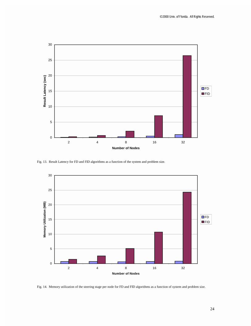
Fig. 13 shows the result latency obtained using the two parallelization schemes. The results confirm that the result latency of FID is much higher than that of FD. This higher result latency is one of the drawbacks of the FID approach.

Another disadvantage of FID, shown in Fig. 14, and one which is likely to prove crucial in embedded sonar systems, is the significantly higher memory capacity required by FID. The higher memory utilization of FID per node is primarily due to the storage space associated with the steering stage. By contrast, FD leads to significant memory savings, because each node only handles some of the frequency bins and thus needs to store the data only for its respective frequency bins. The memory requirement of the steering stage (as well as the other stages) in FD is nearly constant for the range of system and problem sizes considered in this paper.


24

0

5

10

15

20

25

30

2 4 8 16 32

Number of Nodes

Res

ult

Lat

ency

(se

c)

FD

FID

Fig. 13. Result Latency for FD and FID algorithms as a function of the system and problem size.

0

5

10

15

20

25

30

2 4 8 16 32

Number of Nodes

Mem

ory

Uti

lizat

ion

(M

B)

FD

FID

Fig. 14. Memory utilization of the steering stage per node for FD and FID algorithms as a function of system and problem size.


25

7. Conclusions

This work introduces two novel parallel algorithms for robust broadband MVDR beamforming. The sequential baseline is an RB-MVDR algorithm that incorporates broadband processing, a white-noise gain constraint, and CSM inversion using sequential regression. Both the parallel algorithms presented, FD and FID, employ the frequency domain as the basis for parallelization of the sequential baseline.

The two parallel algorithms presented and analyzed provide a promising framework for RB-MVDR beamforming. Both the algorithms exhibit near-linear speedup, with FID performing slightly better as a result of its lower communication time. Both algorithms are observed to be reasonably scalable for increasing problem and system size. As the number of nodes is increased up to 32, the parallel efficiency of FD is decreased from 92% to 79% as a result of its larger and more rapidly increasing all-to-all communication time. By contrast, FID shows a relatively smaller reduction in efficiency from 95% to 86%, due to the relatively smaller impact of the all-to-one communication inherent in FID. However, FID has significantly higher and rapidly increasing memory requirements, whereas the memory utilization of FD is nearly constant as the problem size is increased. For the range of system and problem sizes considered in these experiments, the memory utilization of the memory-intensive steering stage per node is less than 1MB for FD, whereas it increases to nearly 25MB in the case of FID. Therefore, FID would be a more suitable choice for processing systems with sufficient memory for every processor, while FD would be preferable for systems with scalable communication networks, as well as for systems with severe memory constraints.

The selection of a suitable decomposition scheme represents a tradeoff between processing power and memory utilization. Since frequency is the basis for both the parallel algorithms described in this paper, their implementation is independent of the specific details of the individual stages. For example, any CSM inversion technique could be used without requiring modification to the parallelization techniques. Therefore, the methods of parallelization developed in this research are sufficiently versatile to be effectively applied to other beamforming algorithms as well.

Several areas of future research emerge from this work as well as other related work in the area of parallel beamforming algorithms. The parallel algorithms presented in this paper can be extended to split-aperture MVDR beamforming. An implementation of the resulting parallel algorithms for practical adaptive beamforming on an embedded distributed system comprised of low-power DSP devices is also anticipated. Future research would also focus on analysis and parallelization of more advanced adaptive beamforming algorithms that would include main beam and derivative constraints and a near-field wave propagation model. Furthermore, work is needed to analyze the sequential and parallel beamforming algorithms in terms of fault tolerance. Finally, this research provides a foundation for the parallelization of more advanced beamforming algorithms such as Matched Field Processing (MFP) and Matched Field Tracking (MFT).

Acknowledgements

The support provided by the Office of Naval Research on grant N00014-99-1-0278 is acknowledged and appreciated, as is an equipment grant from Nortel Networks. Special thanks go to Thomas Phipps from the Applied Research Lab at the University of Texas at Austin for his many useful suggestions.

References

1. F. Machell, “Algorithms for broadband processing and display,” ARL Technical Letter No. 90-8 (ARL-TL-EV-90-8), Applied Research Laboratories, Univ. of Texas at Austin (1990).

2. H. Krim and M. Viberg, “Two Decades of Array Signal Processing Research, ” IEEE Signal Processing Magazine, July (1996), 67-94.


26

3. M. Zhang and M. H. Er, “Robust Adaptive Beamforming for Broadband Arrays,” Circuits, Systems, and Signal Processing 16(2) (1997), 207-216.

4. L. Castedo and A. R. Figueiras-Vidal, “An Adaptive Beamforming Technique Based on Cyclostationary Signal Properties,” IEEE Trans. on Signal Processing 43(7) (1995), 1637-1650.

5. J. Krolik and D. Swingler, “Multiple Broad-Band Source Location using Steered Covariance Matrices,” IEEE Trans. on Acoustics, Speech, and Signal Processing 37(10) (1989), 1481-1494.

6. H. Cox, R. M. Zeskind, and M. M. Owen, “Robust Adaptive Beamforming,” IEEE Trans. On Acoustics, Speech, and Signal Processing 35(10) (1987), 1365-1377.

7. A. O. Steinhardt and B. D. Van Veen, “Adaptive Beamforming,” International J. of Adaptive Control and Signal Processing 3(3) (1989), 253-281.

8. M. Wax and Y. Anu, “Performance Analysis of the Minimum Variance Beamformer,” IEEE Transactions on Signal Processing 44(4) (1996), 928-937.

9. K. J. Raghunath and V. U. Reddy, “Finite Data Performance Analysis of MVDR Beamformer with and without Spatial Smoothing,” IEEE Transactions on Signal Processing 40(11) (1992), 2726-2735.

10. M. D. Zoltowski, “On the Performance Analysis of the MVDR Beamformer in the presence of Correlated Interference,” IEEE Transactions on Acoustics, Speech and Signal Processing, 36(6) (1988), 945-947.

11. K. Harmanci, J. Tabrikian, and J. L. Crolik, “Relationships Between Adaptive Minimum Variance Beamforming and Optimal Source Localization,” IEEE Transactions on Signal Processing 48(1) (2000), 1-10.

12. S. P. Applebaum and D. J. Chapman, “Adaptive Arrays with Main Beam Constraints,” IEEE Transactions on Antennas and Propagation 24(3) (1975), 650-662.

13. K. Takao, “An Adaptive Antenna Array under Directional Constraints,” IEEE Transactions on Antennas and Propagation 24(3) (1975), 662-669.

14. M. H. Er and A. Cantoni, “Derivative Constraints for Broad-Band Element Space Antenna Array Processors,” IEEE Transactions on Acoustics, Speech and Signal Processing, 31(6) (1983), 1378-1393.

15. M. Moonen, “Systolic MVDR Beamforming with Inverse Updating,” IEE Proc. Part-F, Radar and Signal Processing 140(3) (1993), 175-178.

16. J. G. McWhirter and T. J. Shepherd, “A Systolic Array for Linearly Constrained Least Squares Problems,” Proc. SPIE, Vol. 696 (1986), 80-87.

17. F. Vanpoucke and M. Moonen, “Systolic Robust Adaptive Beamforming with an Adjustable Constraint,” IEEE Trans. On Aerospace and Electronic Systems 31(2) (1995), 658-669.

18. C. E. T. Tang, K. J. R. Liu, and S. A. Tretter, “Optimal Weight Extraction for Adaptive Beamforming Using Systolic Arrays,” IEEE Trans. On Aerospace and Electronic Systems 30(2) (1994), 367-384.

19. S. Chang and C. Huang, “An Application of Systolic Spatial Processing Techniques in Adaptive Beamforming,” J. Acoust. Soc. Am. 97(2) (1995), 1113-1118.

20. W. Robertson and W. J. Phillips, “A System of Systolic Modules for the MUSIC Algorithm,” IEEE Transactions on Signal Processing 41(2) (1991), 2524-2534.

21. A. George, J. Markwell, and R. Fogarty, “Real-time Sonar Beamforming on High-performance Distributed Computers,” Parallel Computing, 26(10) (2000), 1231-1252.

22. A. George and K. Kim, “Parallel Algorithms for Split-Aperture Conventional Beamforming,” J. Computational Acoustics 7(4) (1999), 225-244.

23. K. Kim, A. George, and P. Sinha, "Comparative Performance Analysis of Parallel Beamformers," Proc. of Intl. Conf. on Signal Proc. Apps. and Technology (ICSPAT), Orlando, FL, November 1-4, 1999.

24. K. Kim, A. George, and P. Sinha, "Experimental Analysis of Parallel Beamforming Algorithms on a Cluster of Personal Computers," Proc. of Intl. Conf. on Signal Proc. Apps. and Technology (ICSPAT), Dallas, TX, October 16-19, 2000, accepted and in press.

25. S. Banerjee and P. M. Chau, “Implementation of Adaptive Beamforming Algorithms on Parallel Processing DSP Networks,” Proc. SPIE, Vol. 1770 (1992), 86-97.


27

26. A. George, J. Garcia, K. Kim, and P. Sinha, "Distributed Parallel Processing Techniques for Adaptive Sonar Beamforming," Journal of Computational Acoustics, accepted and in press.

27. P. M. Clarkson, Optimal and Adaptive Signal Processing, CRC Press, 1993.

28. W. H. Press, S. A. Teukolsky, W. T. Vetterling, and B. P. Flannery, Numerical Recipes in C, 2nd ed., Cambridge University Press, 1992.

29. G. H. Golub and C. F. Van Loan, Matrix Computations, 3rd ed., Johns Hopkins University Press, 1996.

30. M. Y. Chern and T. Murata, “A Fast Algorithm for Concurrent LU Decomposition and Matrix Inversion,” Proc. International Conf. on Parallel Processing (1983), 79-86.

31. D. H. Bailey and H. R. P. Ferguson, “A Strassen-Newton Algorithm for High-Speed Parallelizable Matrix Inversion,” Proc. Supercomputing (1988), 419-424.

32. D. S. Wise, “Parallel Decomposition of Matrix Inversion using Quadtrees,” Proc. International Conf. on Parallel Processing (1986), 92-99.

33. V. Pan and J. Reif, “Fast and Efficient Parallel Solution of Dense Linear Systems,” Computers Math. Applic. 17(11) (1989), 1481-1491.

34. B. Codenotti and M. Leoncini, “Parallelism and Fast Solution of Linear Systems,” Computers Math. Applic. 19(10) (1990), 1-18.

35. K. K. Lau, M. J. Kumar, and S. Venkatesh, “Parallel Matrix Inversion Techniques,” Proc. IEEE International Conf. on Algorithms and Architectures for Parallel Processing (1996), 515-521.

36. Message Passing Interface Forum, “MPI: A Message-Passing Interface Standard,” Technical Report CS-94-230, Computer Science Dept., Univ. of Tennessee, April 1994.

37. D.E. Culler and J.P. Singh, Parallel Computer Architecture: A Hardware/Software Approach, Morgan Kaufmann Publishers Inc., San Francisco, CA, 1999.

Documents

PARALLEL ALGORITHMS FOR ROBUST …ufdcimages.uflib.ufl.edu/UF/00/09/46/60/00001/JCA2001.pdfPARALLEL ALGORITHMS FOR ROBUST BROADBAND MVDR BEAMFORMING PRIYABRATA SINHA, ALAN D. GEORGE