Embed Size (px)
Citation preview

DI
SC
US
SI
ON
P
AP
ER
S
ER
IE
S
Forschungsinstitut zur Zukunft der ArbeitInstitute for the Study of Labor
Pappa Ante Portas:The Retired Husband Syndrome in Japan
IZA DP No. 8350
July 2014
Marco BertoniGiorgio Brunello

Pappa Ante Portas:
The Retired Husband Syndrome in Japan
Marco Bertoni University of Padova
and CEP, LSE
Giorgio Brunello University of Padova
and IZA
Discussion Paper No. 8350 July 2014
IZA
P.O. Box 7240 53072 Bonn
Germany
Phone: +49-228-3894-0 Fax: +49-228-3894-180
E-mail: [email protected]
Any opinions expressed here are those of the author(s) and not those of IZA. Research published in this series may include views on policy, but the institute itself takes no institutional policy positions. The IZA research network is committed to the IZA Guiding Principles of Research Integrity. The Institute for the Study of Labor (IZA) in Bonn is a local and virtual international research center and a place of communication between science, politics and business. IZA is an independent nonprofit organization supported by Deutsche Post Foundation. The center is associated with the University of Bonn and offers a stimulating research environment through its international network, workshops and conferences, data service, project support, research visits and doctoral program. IZA engages in (i) original and internationally competitive research in all fields of labor economics, (ii) development of policy concepts, and (iii) dissemination of research results and concepts to the interested public. IZA Discussion Papers often represent preliminary work and are circulated to encourage discussion. Citation of such a paper should account for its provisional character. A revised version may be available directly from the author.
IZA Discussion Paper No. 8350 July 2014
ABSTRACT
Pappa Ante Portas: The Retired Husband Syndrome in Japan* The “Retired Husband Syndrome”, that affects the mental health of wives of retired men around the world, has been anecdotally documented but never formally investigated. We use Japanese micro data and the exogenous variation generated by the 2006 revision of the Japanese Elderly Employment Stabilization Law, which mandated employers to guarantee continuous employment between mandatory retirement age and full pension eligibility age, to estimate the causal effect of the husband’s retirement on the wife’s mental health. We find that adding one year to the time spent in retirement by Japanese husbands increases the probability that their wives develop the syndrome by 5.8 to 13.7 percentage points, depending on the empirical specification. We discuss mechanisms at work and argue that – ceteris paribus – increasing female labour force participation might exacerbate rather than attenuate the phenomenon. JEL Classification: D1, I1, I3, J14, J26 Keywords: retirement, pension reforms, couples, stress, depression, Japan Corresponding author: Giorgio Brunello Department of Economics and Management “Marco Fanno” University of Padova Via del Santo 33 35123 Padova Italy E-mail: [email protected]
* Pappa Ante Portas is a 1991 German movie directed by Loriot and Renate Westphal-Lorenz, describing the conflicts between a retired husband and his wife and son. The title alludes to Hannibal ante portas! (“Hannibal before the gates!”), a Roman call referring to Carthaginian commander Hannibal on his way to Rome in 211. This research uses micro data from the Preference Parameters Study of Osaka University’s 21st Century COE Program ‘Behavioral Macrodynamics Based on Surveys and Experiments’ and its Global COE project ‘Human Behavior and Socioeconomic Dynamics’. We are grateful to Yoshiro Tsutsui, Fumio Ohtake, and Shinsuke Ikeda for providing the data, to Kenn Ariga, James Banks, Tabea Bucher-Koenen, Morten Schuth, Guglielmo Weber for comments and the audiences at the workshop on “Population Ageing: Economics, Health, Retirement and the Welfare State” in Padova and at a seminar at the Munich Center for the Economics of Ageing (MEA), where Marco Bertoni was a visitor when the paper was drafted, for useful suggestions. Financial support by the POPA_EHR strategic research project of the University of Padova is gratefully acknowledged. The usual disclaimer applies.

2
1. Introduction
"I am going nuts", "I want to scream", "He is under my feet all the time", "He his driving me crazy", "I'm
nervous", "I can't sleep". These expressions, reported by Johnson, 1984, describe the "Retired Husband
Syndrome" (RHS hereafter) of some of his middle-aged American female patients, whose husbands
have recently retired. Johnson’s clinical description of the symptoms of this stress-induced condition
includes headaches, depression, agitation, palpitations, and lack of sleep.
Anecdotal evidence on the syndrome has been reported by several leading newspapers and TV
networks, including The Washington Post, the BBC and Forbes.1 While stories about the RHS are by
no means restricted to a single country, the international public debate has focused mainly on Japan,
because of its alleged diffusion there. A BBC report suggests that over 60 percent of older Japanese
women are affected by the syndrome, with soaring divorce rates.2
The diffusion of RHS in Japan has been often related by the press to its economic and social fabric.
Although labour force participation of married females in Japan has increased during the past decades
(see Ogawa and Ermisch, 1996; Sasaki, 2002; Abe, 2013), many Japanese married women still
concentrate on household work, including child-care, as full-time housewives.3 In the strict division of
labour within the family that still survives in Japan, wives stay at home and husbands spend their long
working hours as well as leisure time after work with colleagues and away from home. After a life apart
and progressive estrangement, many Japanese couples are forced to start spending time together when
the husband retires. This can be a very stressful experience for wives, who suddenly have to face the
continuous presence of a stranger in the house and the additional burden of his requests.
In spite of the interest sparked by the media on the syndrome, and of its potential relevance for the
well-being and health of older married women, little empirical evidence exists to date documenting the
presence of a causal relation between the husband’s retirement and the wife’s unhappiness, and
establishing how sizeable the eventual effect is.4 In this paper, we try to fill this gap by focusing on the
wife’s mental health – measured by stress, depression, and lack of sleep.
Our data are drawn from the Preference Parameters Study (PPS), an annual survey conducted by the
University of Osaka on a representative sample of the Japanese population, which contains detailed
information on individuals and their spouses, including retirement, divorce and self-reported measures
of depression, stress and lack of sleep. The causal impact of the husband’s retirement is identified using
1 Laura, R., Can Your Marriage Survive Retirement?, Forbes, 1/24/2013; Kenyon, P., Retired Husband Syndrome, BBC, 11/13/2006; Faiola, A., Sick of Their Husbands in Graying Japan, The Washington Post, 10/17/2005. 2 In Japanese, this syndrome is called Shujin Zaitaku Sutoresu Shoukougun (主人在宅ストレス症候群), or "stress syndrome from having the husband at home”. 3 In a recent study, Steinberg and Nakane, 2012, report that the gender gap in prime – age labour force participation in 2009 was 25 percent in Japan, 14.1 percent in the US and 12.2 percent in Germany. 4 An important recent exception is Stancanelli, 2014, who studies the effects of retirement on divorce using French data.

3
the exogenous variation generated by the 2006 revision of the Japanese Elderly Employment
Stabilization Law (see Kondo and Shigeoka, 2014), which mandated Japanese employers to guarantee
continuous employment between mandatory retirement age (at age 60) and full pension eligibility age.
This law created a discontinuity between the cohorts of males born after 1945, who turned 60 in 2006
or later and had the opportunity to continue employment until full pension eligibility age and the
cohorts born between 1940 and 1945, who were guaranteed employment only until mandatory
retirement at age 60, before full pension eligibility age.
In line with what reported by the press and the clinical literature, we find that the husband’s
retirement affects the wife’s RHS symptoms by increasing her stress, depression and inability to sleep.
The size of the effect is sizeable: we estimate that, conditional on the age of both partners as well as on
the husband’s cohort of birth, adding one year to the time spent in retirement by the husband increases
the probability that the wife develops RHS symptoms by5.8 to 13.7 percentage points, depending on
the estimation method.
We show that candidate mechanisms explaining why the husband’s retirement affects the wife’s
mental health include the presence of elderly parents in the household and low financial wealth. These
mechanisms account for about one fifth of the total effect. Perhaps surprisingly, given the scant
attention devoted to this fact by the media, we also find that the husband’s retirement has similar
effects on the mental health of both partners, suggesting that the husband’s RHS symptoms may be
another candidate mechanism explaining the wife’s symptoms.
Last but not least, our estimated effects are stronger for employed women, who are already stressed
by their job and have less time to comply with the additional requests of their retired husbands,
suggesting that low female labour force participation may contribute to attenuate rather than exacerbate
the diffusion of RHS in Japan. Overall, our results highlight the importance of studying retirement as a
joint process affecting the couple, as failure to consider cross-partner effects may lead to
underestimating the negative consequences of retirement on mental well-being.
The paper unfolds as follows. Section 2 reviews the relevant economic literature; Sections 3 and 4
describe the institutional background and our empirical strategy. We introduce our data in Section 5.
Results and potential mechanisms are discussed in Section 6. Conclusions follow.
2. Literature review
This paper brings together two research strands in the economics of ageing: the analysis of the
effects of retirement on the retiring individual’s mental health, and the study of the implications of
retirement on other individuals, including the partner.
4
The effects of retirement on the mental well-being of the retiring individual are not yet fully
understood. While Charles, 2004, and Johnston and Lee, 2009 report that retirement reduces
depression and increases subjective well-being in the US and the UK, other contributions in this
literature do not point unambiguously in the same direction. Both Lindeboom et al., 2002, and Clark
and Fawaz, 2009, for instance, fail to find retirement effects on mental health, respectively for the US
and Europe. On the other hand, Kim and Moen, 2002, contrast the positive short-term "honeymoon"
effects with the negative longer-run effects in the US, and Börsch-Supan and Jürges, 2009, find that
German early retirees are generally less happy than those still working. Bonsang and Klein, 2012, show
that in Germany the lack of a significant relationship between overall life satisfaction and retirement is
the outcome of the combined positive and negative relationship with satisfaction with leisure and
income, respectively, and that involuntary retirement due to plant closures does instead lead to a
significant decrease in overall life satisfaction.
The effects of retirement could spill-over from the individual to others with whom the individual
interacts, for instance the partner. The economic literature has provided so far little evidence on cross-
partner retirement effects, by focusing mainly on the joint retirement decision of couples. An early
study in this area is Hurd, 1990, who found that the timing of retirement of husbands and wives are
positively correlated in the US.
Additional research by Blau, 1998; Blau and Gilleskie, 2006; Casanova, 2010; Gustmann and
Steinmeier, 2000, 2004; and Michaud, 2003, models the retirement process in the household and
highlights two main channels of cross-partner retirement effects: budget constraint and
complementarities in leisure effects. Coile, 2004a, investigates how couples respond to retirement
incentives in the US, and reports that husbands are more responsive to wives' social security incentives
than vice-versa. She highlights that complementarities of leisure may be asymmetric across partners,
with husbands enjoying joint leisure more than wives do. In their comparison of the retirement
behaviour of British and American couples, Banks, Blundell and Casanova, 2010, find that British men
are more likely to react to their wives’ retirement incentives than their American counterparts.
Conversely, Hospido and Zamarro, 2014, use data for continental Europe and show that while women
tend to leave the workforce when their husbands retire, the opposite does not hold. 5 Finally,
Stancanelli, 2012; Stancanelli and Van Soest, 2012a, 2012b; and Stancanelli, 2014, show that reaching
minimum retirement age in France has cross-partner effects on the incidence of divorce, joint leisure
and home production.6
5 Bloemen, Hochguertel and Zweerink, 2014, present similar evidence for the Netherlands. 6 Descriptive studies on the cross-partner health effects of retirement have been conducted by psychologists (see Smith and Moen, 2004, Szinovacz, 1980, Szinovacz and Davey, 2004, 2005).

5
There are also studies documenting that cross partner effects involve also other life events, most
notably unemployment. For instance, Charles and Stephens, 2004, find that unemployment has a
positive effect on divorce rates in the US, and Marcus, 2013, reports that unemployment in Germany
reduces the spouse’s as much as the individual’s happiness.
In one of the few Japanese studies we are aware of, Sugisawa, Sugisawa, Nakatani and Shibata, 1997,
use a representative sample of Japanese individuals aged 60+ and find no evidence that retirement is
significantly related to either mental health or to the degree of social participation. In a more recent
study, Hashimoto, 2013, uses the Japanese Study of Ageing and Retirement (JSTAR) and finds that
psychological distress and cognitive functioning decline after retirement for men but not for women.
Furthermore, retirement is accompanied by increased social participation, which improves
psychological distress and delays cognitive decline among men but not among women. These two
studies have two common features: a) they consider the effects of retirement on the retiring individual’s
health but ignore the effects on the partner; b) by failing to address the endogeneity of the retirement
decision in health regressions, they cannot recover causal effects. These are important shortcomings,
that we address in the current study.
3. Institutional Background
In Japan, long term employment contracts typically terminate with mandatory retirement. Because
of population ageing, the government established in 1986 that firms had to extend mandatory
retirement age from 55 to 60 (Shimizutani and Oshio, 2010), but tolerated ages below 60 until 1998
(Kondo and Shigeoka, 2014). Starting from 2013, mandatory age is expected to increase to 61, and will
eventually reach age 65 by 2025.
The two-tier pension scheme for private sector employees – see Okumura and Usui, 2014, for an
overview - was reformed by the 2001 Pension Reform Act, which gradually increased the minimum
eligibility age for full pension benefits above mandatory retirement age. For men, and starting in 2001,
the cohorts born between 1941 and 1943 could draw the flat-rate pension benefit (first tier) only from
age 61, while retaining the right to draw the wage proportional benefit (second-tier) from age 60.
Younger cohorts were progressively exposed to even higher increases in the minimum eligible age for
the flat-rate component of pension benefits, until age 65 was reached in 2013 for the cohorts born in
1949 or later (see Table 1 in Okumura and Usui, 2014 for further details).7
Before 2006, the increase in the minimum eligible age for the first tier of pension benefits was not
accompanied by changes in mandatory retirement age. Therefore, individuals belonging to the exposed
7 See also Ichimura and Shimizutani, 2012. Kondo and Shigeoka, 2014, report an average share of the first tier component to total pension benefits equal to 37.5 percent.

6
cohorts reached mandatory age without being able to draw full pension benefits. To address this
problem, the Japanese government passed in 2006 a revision of the Elderly Employment Stabilization
Law (EESL), which mandated firms to introduce measures to continue employment until eligibility for
full pension benefits was reached. This additional reform affected private sector employees born from
1946 onwards, by raising the maximum age of guaranteed employment from 60 to 63 for those born in
1946, to 64 for those born between 1947 and 1948, and to 65 for those born from 1949 onwards (see
Kondo and Shigeoka, 2014, Table 2). To illustrate with an example the consequences of the EESL
revision, consider two employees born in 1945 and 1946. For the former, maximum guaranteed
employment and full pension eligibility age were 60 and 63 respectively. For the latter, both ages were
set at 63.
Firms could comply with the employment guarantee either by raising mandatory retirement age, a
costly option given the steeply rising age-earnings profiles in Japan, of by re-employment after
mandatory retirement until guaranteed age, typically at a lower wage. To further encourage retention,
the government provided a subsidy to employers who offered re-employment to all retiring employees.8
Not surprisingly, as of 2008 roughly 15 percent of employers chose to extend mandatory retirement,
and the remaining 85 percent selected re-employment.
Importantly, the practice of re-employing workers after mandatory retirement pre-dates the revision
of the Law. According to the “Personnel Management Survey” (Koyo Kanri Chosa) conducted in 2004,
67.5 percent of Japanese firms had a re-employment system after mandatory retirement. Of these,
however, only 15.7 percent continued to employ all those who wished to be employed after reaching
age 60. Employment opportunities for older workers increased after the EESL revision, which also
compelled firms with more than 50 employees to report on the implementation of measures for
continued employment in June of each year.
By June 2007, close to 93 percent of reporting firms had implemented these measures. According to
a survey carried out by the Ministry of Health, Labour and Welfare and quoted by Fujimoto, 2008, two
thirds of these firms reported that they employed almost all those who wished to stay on, a substantial
increase with respect to the years before 2006. The rest employed between 70 and 90 percent of
applicants. Selection of applicants was based on eligibility requirements, such as good health, attitude,
attendance and performance. Fujimoto, 2008, reports the results of a government survey suggesting
that the number of regular employees aged 60 to 64 and 65+ increased by 26.9 and 46.5 percent,
respectively, because of the EESL revision.
4. Our Empirical Approach
8 We are grateful to Kenn Ariga for providing this information.

7
We estimate the effect of the husband’s retirement on the wife’s mental health using the following
empirical model:
(1)
where is mental health of the wife in couple j at time t, and are the husband’s current
and retirement age, is equal to the number of years spent in retirement plus 1 if the husband has
already retired and to zero otherwise,9 or more formally:
01
(2)
, and are controls for the couple, the wife and the husband and is the error term. In our
baseline specifications, includes the number of children and the education of both partners, is
the wife’s age and the husband’s age and cohort of birth. Since our data include repeated
observations for individuals, we cluster standard errors at the individual level.
The estimation of equation (1) by OLS is unlikely to uncover causal effects for at least three reasons.
First, the husband's retirement is a choice variable, which is likely to be affected by the wife’s mental
health.10 Second, there could be measurement error in the husband's retirement status - that does not
necessarily measure disengagement from work. Last but not least, there may be omitted variables in
equation (1) that affect both the husband's retirement and the wife's mental health.
We address these problems using an IV (instrumental variables) identification strategy. To qualify as
valid, the candidate instrument should affect the wife’s mental health only via its impact on the
husband’s retirement, and should therefore be uncorrelated with variables entering in the error term of
equation (1), such as the wife's employment status. Similarly to Kondo and Shigeoka, 2014, our selected
instrument exploits the discontinuity across cohorts induced by the revision of the EESL in 2006,
which guaranteed additional employment after age 60 to the cohorts born between 1946 and 1952
(treated cohorts), but not to earlier cohorts born between 1940 and 1945 (control cohorts). Prima facie
evidence on the effect of the EESL reform is shown in Figure 1. Using the data described in the next
section, we plot the percentage of retired husbands by cohort of birth (1940 to 1952). The figure shows
a large discontinuity in this percentage – from close to 38 to close to 20 percent – around the critical
9 See Peracchi and Mazzonna, 2012, for a similar definition. We add 1 to current age to avoid assigning the same value to those who have just retired (age equal to retirement age) and those who have still to retire. 10 For instance, Coile, 2004b, shows that in the US the husband’s labour supply is positively affected by negative health shocks affecting the wife.

8
cohort of individuals born in 1946, who were first affected by the EESL amendment, suggesting that
the reform has been quite effective in delaying the retirement of older Japanese men.
Since our data are longitudinal, we maximize the variability of the instrument between individuals
and for each individual over time by defining it as
01
(3)
where is the age of the husband born in year c who belongs to couple j at time t and is the
maximum age of guaranteed employment for employees born in cohort c. The variable is equal to
zero whenever individual age is below maximum age CEG, and equal to the distance between age and
CEG plus 1 when individual age is above or equal to the maximum age.11 The discontinuous jump in
CEG, from 60 to 63 for those born in 1946, from 60 to 64 for those born between 1947 and 1948 and
from 60 to 65 for those born later, generates discontinuous jumps in Z. To illustrate, consider
individuals aged 64 who have been born between 1944 and 1948. Their value of Z is equal to 5 for
those born in 1944 and 1945, falls to 2 for those born in 1946 and further to 1 for those born in 1947
and 1948.
Our identification strategy requires that the instrument is uncorrelated with the error term in
equation (1), which includes the wife’s employment status. Although this assumption is not testable,
Figure 2 is clearly supportive as it shows that – contrary to the case of husband’s retirement – there is
no detectable discontinuity in the wife’s labour force participation12 as we move from untreated to
treated husband’s cohorts.13 A further threat to identification is that, because of data restrictions, we
consider married couples only. However, the husband’s retirement could be so stressful for the wife to
induce divorce (see Stancanelli, 2014). By omitting divorced wives from the sample, we are likely to
underestimate the effect of the husband’s retirement on the wife’s mental health. We identify divorced
males in our data14 and plot the divorce rate by cohort of birth in Figure 3. The figure shows no clear
discontinuity in the neighbourhood of the pivotal cohort that was first affected by the revision of the
EESL Law, indicating that our instrument is orthogonal to selection into marriage.
11 As in the case of YR, we add 1 to individual age to avoid assigning the same value of Z to both treated individuals with age equal to CEG and untreated individuals with age less than CEG. 12 Hashimoto, 2013, suggests that the retirement process of Japanese females often involves transiting to homemaking and non-employment as alternatives to formal retirement. We therefore use an indicator of labour force participation rather than simply retirement. 13 Formal statistical evidence on this point is provided later in the paper. 14 As clarified in the next section, where we present our data, we need to focus on divorced males because we do not have information on husbands’ date of birth for divorced women.

9
We estimate Equation (1) both by Two Stage Least Squares (2SLS) and using an IV probit model, to
account for the fact that the dependent variable MH is binary. IV methods capture the local average
treatment effect of the husband's retirement on the wife's mental health for the sub-population of
compliers affected by the EESL reform (see Imbens and Angrist, 1994). Before this reform, re-
employment programs were adopted by firms on a discretionary basis. It seems plausible to assume
that, during this period, firms were less willing to offer re-employment to the less talented and skilled.
After the Law was revised in 2006, these programs were extended to cover all workers, and
economic incentives were provided to employers choosing to do so. Many offered the employment
guarantee to all applying workers, and some conditioned the guarantee to a few eligibility requirements,
including performance. This suggests that the compliant sub-population consisted of workers with
lower performance, who in some cases met a minimum requirement. Our estimated effects are
informative of the marginal improvement in the wife’s mental health when this sub-group is induced by
the EESL to stay longer at work rather than retire.
5. Data
We use data from the Japanese Preference Parameters Study (PPS), conducted by the University of
Osaka. The PPS is a nationally representative panel survey on behaviours, risk attitudes, habits
formation and time preferences of the Japanese population, carried out yearly from 2003 onwards, with
refreshment samples in 2006 and 2009. Interviews are carried out via paper-and-pencil questionnaires
that are delivered and picked up by interviewers at the interviewees' homes, with very high response
rates (always above 70% and in recent years close to 90%) in both the longitudinal and the refreshment
samples.15
The PPS is not a household survey, as only one individual per household is interviewed. However,
the questionnaire asks married interviewees to report information on their partners as well, including
year of birth, education, employment status and, if the partner is retired, age at retirement. Since we are
interested in studying how the husband’s retirement affects the wife’s mental health, we consider the
sub-sample of interviewed married females, who provide information on both key variables. As the
annual questionnaire includes a common set of questions as well as wave-specific questions, we can
only use the waves from 2008 to 2013. In these waves interviewees were asked how they felt about the
following statements describing their mental health:
- I have been feeling stressed lately.
15 These data have been used, among others, by Horioka, 2014, to study bequests, by Hanaoka et al., 2014, to study the effects of earthquakes on preferences, and by Brunello and De Paola, 2013, to study the effects of siblings composition on leadership.

10
- I have been feeling depressed lately.
- I haven’t been sleeping well lately.
Responses had to be provided on a 5-point discrete scale, with 1 indicating something particularly true
for the respondent and 5 something that does not hold true at all for the respondent. The evaluations of
these statements provide useful information on key symptoms of RHS, as described by Johnson, 1984,
in his clinical article. We recoded each of the three variables as dummies equal to 1 for values 1 and 2
of the original answers, and to 0 otherwise. Our main dependent variable is the dummy RHS (Retired
Husband Syndrome), equal to 1 if at least one of the three dummy variables just described is equal to 1,
and to 0 otherwise.16
Our data include also information at the household level, such as the number of children, the
presence of the parents in the household – both of the respondent and of the respondent’s husband,
homeownership, household net income and household financial assets (both variables are recoded as
dummy variables equal to 1 if the household belongs to the bottom three deciles of the income and
wealth distribution in the sample, and 0 otherwise), and whether the household has debts. Finally, from
2010 onwards we have also information on the average daily minutes spent by wives doing house
chores.
Our sample consists of married women whose husbands were born between 1940 and 1952, a six-
years span on each side of the 1946 cohort, first affected by the 2006 EEPL reform. We drop outliers
in the distribution of the age difference between partners by excluding married couples where the wife
was born either before 1940 or after 1961, which are around two percent of the initial sample. Our final
sample consists of 836 wives, each observed multiple times in the panel, for a total of 3,288 wife-year
observations with non-missing values in the outcome and treatment variables.
Descriptive statistics for the relevant variables are shown in Table 1. It turns out that 47 percent of
the wives in our sample report RHS symptoms: 41 percent have been feeling stressed, 23 percent have
been feeling depressed and 16 percent haveexperienced sleeping difficulties. On the one hand, 23
percent of husbands are retired, with 6.1 average years since retirement (conditional on retirement). On
the other hand, 51 percent of husbands are older than the cohort – specific maximum guaranteed
employment age, with an average distance from that age equal to 7.2 years, conditional on eligibility.
6. Results and Discussion
Our identification strategy relies on the exogenous variation provided by the changes in maximum
guaranteed employment age (CEG) across contiguous cohorts. We start the presentation of our results
16 We have experimented with several alternative specifications of the dependent variable, but results are always qualitatively similar.

11
by illustrating in Table 2 the first stage effects of the instrument Z both on YR, the number of years
spent in retirement by the husband, and on the wife’s labour force participation.
As shown in Column (1) of the table, we find that, conditional on the wife and the husband’s age,
the husband’s year of birth, the education of both partners and the number of children in the
household, the instrument Z has a positive and statistically significant effect on YR. We estimate that
one additional year in the gap between current age and maximum age of guaranteed employment
increases time into retirement by 0.361 years, a sizeable effect.17 As documented by the Angrist -
Pischke first stage F statistic – equal to 75.4 – our instrument is not weak. To verify the quality of the
data reported by wives on their husbands, we also estimate the effect of the instrument on the gap
between current and retirement age as reported by the husbands on themselves rather than by their
wives and find very similar results.18
Reassuringly for our identification strategy, Column (2) reports that the instrument Z is unrelated to
the wife’s labour force participation, thereby confirming the descriptive evidence of Figure 2. As a
further identification test, we follow Bingley and Martinello, 2013 and regress predetermined variables
such as education and the number of children on the instrument, husband’s age and cohort and wife’s
age. Table A1 in the Appendix provides further support on the validity of our instrument by showing
no statistically significant effect.
We report in Table 3 the reduced form estimates, using as dependent variables the dummy RHS and
separate dummies for stress, depression and lack of sleep. Conditional on linear trends in age and
cohorts19 and on both partners’ education and number of children, we estimate that one additional year
in the gap between current husband’s age and the maximum age of guaranteed employment increases
the likelihood of having a wife with RHS symptoms by 2.1 percentage points, a 4.5 percent increase
with respect to the sample average (0.46). When we break down these symptoms, we find that the
highest percentage effect is on stress, and the lowest on depression. The differences between these
effects, however, are not statistically significant.20
The OLS, 2SLS, probit, and IV probit estimates of Equation (1) are reported in Table 4, where we
show the marginal effects of adding one year to the husband's retirement on the wife's RHS symptoms.
17 This effect is partly due to the increase in the probability of retirement, which rises by 2.7 percentage points, a 12 percent increase with respect to the average sample probability (0.23). Our first stage estimates are robust to several specification changes, which include the use of cohort dummies rather than a cohort trend, and the use of second order polynomials for age and cohort trends. 18 When retirement age and status is reported by the husbands, the estimated first stage effect of Z is 0.290, slightly lower but not statistically different at the conventional levels of significance from the first stage effect when these variables are reported by the wives (the p-value of the test for equality of the two first stage coefficients is 0.278). When we pool both samples – those with data reported by wives and husbands - the first stage effect of Z is 0.326, and the F statistic is equal to 101. 19 We have experimented with quadratic trends and with cohort dummies for the reduced forms as for the first stage, but found that linear trends give the best fit. 20 We estimate the three equations using SURE and test whether the coefficients associated to Z are statistically different. We never reject the null of no difference.

12
Separate results for stress, depression and lack of sleep are presented in Table A2 in the Appendix.
Considering first the OLS and probit specifications, reported in Columns (1) and (3) respectively, we
find no evidence that husband’s retirement and wife’s RHS are associated, as marginal effects are close
to zero and not statistically significant in either estimate. When we address the endogeneity of
retirement in Columns (2) and (4) of the table, however, our estimates change markedly: we find that,
conditional on the usual covariates, the husband’s retirement has a positive and statistically significant
causal effect on the wife’s RHS symptoms.21 The estimated marginal effects are sizeable: conditional on
the wife’s age, adding one year to the duration of the husband’s retirement increases the probability that
the wife develops RHS symptoms by 5.8 to 13.7 percentage points, a 12 to 29 percent increase with
respect to the sample average value (0.47).22
A candidate explanation of the large gap between the OLS and 2SLS (and between probit and IV
probit) estimates of the husband’s retirement effect is the presence of substantial attenuation bias due
to measurement error in reported retirement status, a common event in the literature on the effects of
retirement on health (see e.g. Celidoni, Dal Bianco and Weber, 2013). Another candidate is endogenous
selection: if the husbands whose wives are not depressed select into earlier retirement, this would
impart a negative bias on the OLS estimates, reducing them below the consistent 2SLS estimates.
Finally, in the presence of heterogeneous effects, the gap in the estimates could reflect the fact that
OLS and 2SLS yield a population average treatment effect (ATE) and a local average treatment effect
(LATE) respectively, where the latter is the effect for the sub-group of complying husbands, who have
been granted additional employment after age 60 because of the revision of the Law. Since firms could
re-employ older workers on a voluntary and selective basis even before the 2006 Law, we expect that
those offered re-employment before the reform belonged to the sub-group of applicants with better
health, attendance and performance. After the reform, firms had to set up plans to offer re-
employment to other workers as well. Some that did so introduced eligibility criteria to avoid employing
workers with few desirable characteristics. Others offered re-employment to all workers and were
compensated by the government with monetary incentives. Our interpretation is that the reform
induced many firms to keep in their ranks the group of older workers whom would not have been kept
in the absence of the law, because their health, attendance and performance were above a minimum
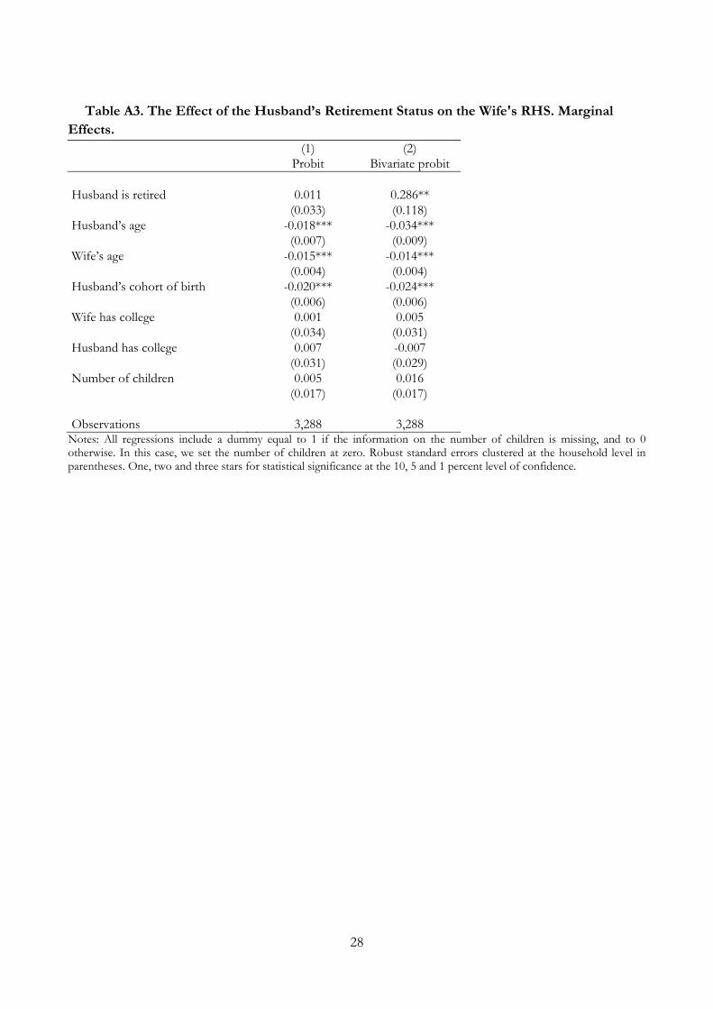
21 Similar results are obtained using Two-Samples 2SLS (see Inoue and Solon, 2010). This estimator combines the first stage estimated in the pooled sample of husbands reporting information on their retirement and wives report information on their husband’s retirement with the reduced form estimated in the subsample of wives who report on their RHS symptoms. The estimated marginal effect is 0.064 (standard error: 0.026). 22 We report in Table A3 in the Appendix the probit and bivariate probit estimates of the effects of the husband’s retirement status - rather than duration into retirement - on the wife’s RHS symptoms, and find evidence of a positive and statistically significant effect. As pointed out by Nichols, 2011, the bivariate probit model estimates require both stronger parametric assumptions and the assumption that the estimated treatment effect is constant. Under these assumptions, this method provides efficient estimates of the average treatment effect.

13
threshold but still relatively low. The estimates reported in Table 4 suggest that delaying the retirement
of this group has had a substantial positive effect on their wives’ mental health.
We further investigate the presence of heterogeneous effects by estimating the impact of the
husband’s retirement of the wife’s RHS symptoms separately for husbands with and without a college
degree. Both the 2SLS and the IV probit estimates reported in Table 5 show that marginal effects are
positive for both groups but higher when the husband does not have a college degree, although
estimated differences are not statistically significant in the standard sense.23
We have documented that the husband’s retirement has a causal effect on the wife’s RHS
symptoms, measured by stress, depression and lack of sleep. In the rest of this section, we investigate
mechanisms that could explain these results. One mechanism is that retired husbands place additional
demands on their wives’ time, thereby increasing stress and other symptoms. If this is the case, we
expect to find that retirement affects RHS to a higher extent for working than for non-working wives,
mainly because the former have tighter time constraints than the latter. In support of this, we estimate
our key equation separately for working and non-working wives and find that the impact of retirement
on RHS is indeed higher among working wives – see Table 6.24 This result suggests that – ceteris
paribus – increasing the labour force participation of Japanese married females might exacerbate rather
than attenuate the diffusion of RHS in Japan.
In addition, the husband’s retirement may influence household composition, income and wealth,
which in turn affect the wife’s well-being. As documented in Table A4 in the Appendix, the husband’s
retirement increases the likelihood that elderly parents live in the household. The attention and care
required by these parents is likely to increase pressure on the wife, leading to either more stress, lack of
sleep or higher depression. We also document that retirement is associated to lower financial security,
an obvious source of stress for both partners. Following Cutler and Lleras-Muney, 2010, we explore the
mediating contribution of these variables by adding them to Equation (1) and by verifying whether
their inclusion alters the estimated effect of the husband’s time since retirement on the wife’s RHS
symptoms. As shown in Table 7, the inclusion of these covariates reduces the estimated effect of the
husband’s retirement on the wife’s RHS symptoms, which declines by 18 to 23 percent, depending on
the estimation method. Therefore, differences in household composition, income and wealth account
for about one fifth of the entire effect.
Another potential mechanism – that we have hinted at when discussing the effects of retirement on
employed and not employed wives – is the increased time spent by the wife doing housework.
Stancanelli and Van Soest, 2012, examine data for France and find that the wife’s retirement
23 We formally test for differences in the parameters by jointly estimating the equations for husbands with and without a college degree. 24The difference in the estimated parameters is statistically significant at the 10 percent level of significance (p-value: 0.078)

14
substantially reduces the husband’s time spent doing housework. The opposite, however, does not
hold. While we do have information in our data on time spent by both partners doing housework,
unfortunately this information is only available for a few waves. Hence, due to the small sample size we
typically find statistically insignificant effects of retirement on housework, and of housework on RHS
symptoms.25
Finally, a candidate source of the wife’s RHS symptoms is that the husband himself experiences
these symptoms because of his own retirement. While our data allow us to match the wife’s RHS to the
husband’s retirement status and duration, this is not possible for the husband’s RHS symptoms.
Therefore, we cannot assess whether this is an important mechanism by adding it to the set of
covariates in Equation (1), as done in Table 7. We report, however, the impact of time since retirement
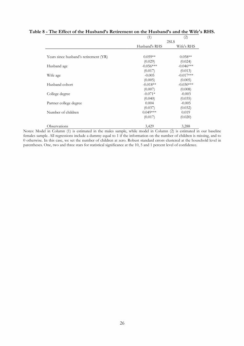
on the RHS symptoms of both partners – see Table 8 – and show that the estimated effects are almost
identical, suggesting that concern with the “Retired Husband Syndrome” should not be limited to
wives, as both partners are affected.
Last but not least, retired husbands may be in poorer health, even after controlling for age, and in
need of assistance and care, which is often provided by the wife. While we do have data on self-
reported health, this information is available only for the last three waves. Unfortunately, because of the
limited number of observations, our estimates on the effects of the husband’s retirement on the health
of both partners are too imprecise for us to reach any conclusion on this potential mechanism.
Conclusions
This paper provides the first empirical evidence on the causal effect of the husband’s retirement on
the wife’s mental health, the so called “Retired Husband Syndrome”, affecting the stress, depression
and ability to sleep of married women with retired husbands. Our evidence is from Japan, a country
that has attracted considerable press attention on this matter. The diffusion of RHS in Japan has been
often related to its economic and social fabric. In this country, the persistence of traditional gender
roles has been seen as exacerbating the syndrome, because Japanese wives tend to spend most of their
life at home taking care of the husband, the house and the kids, and Japanese husbands spend long
hours at work and with their colleagues, and very little time at home with their wives.
We have estimated the causal effect of the husband’s retirement on the wife’s health using
longitudinal data from the Osaka University Preferences Parameter Study, a survey particularly suitable
for our purposes because it collects detailed information on preferences, behaviours and labour market
status of both partners in the household. We have addressed the endogeneity of the husband’s
retirement using the exogenous variation generated by changes in the maximum age of continuous 25 Results of these estimates are available from the authors upon request.

15
guaranteed employment - produced by the 2006 revision of the EESL Law - which affected only the
cohorts born after 1945.
In line with what reported by the press and the clinical literature, we have found that the husband’s
retirement and its duration significantly affected the wife’s RHS, measured by increased stress, higher
depression or inability to sleep. We have estimated that adding one year to the time spent by the
husband in retirement increases the probability that the wife develops RHS symptoms by 5.8 to 13.7
percentage points, a sizeable effect.
We have found that retirement effects are stronger for employed women, who are already stressed
by their job and have less time to comply with the additional requests by their retired husbands. This
result casts some doubts on the view that low female labour force participation is a key factor in the
diffusion of RHS in Japan, and suggests that – ceteris paribus - rising participation might further
increase the incidence of the syndrome. Moreover, we have presented evidence showing that both low
financial wealth and the presence of elderly parents in the household are mechanisms relating the cause
(husband’s retirement) to the effect (wife’s RHS), accounting for about one fifth of the total effect.
We have also found a quantitatively similar effect of the husband’s retirement on his own mental
health. Rather surprisingly, this aspect of the RHS syndrome has not attracted the same attention from
the press and the general public. While we suspect that the husband’s RHS might be an important
mechanism explaining the wife’s RHS, the nature of our data does not allow us to further investigate of
this point. Needless to say, this question must be left to future research and to better data.
Our results highlight the need to study retirement as a joint process affecting the couple, and show
that failure to consider cross partner effects can lead to underestimate the negative consequences of
retirement on mental well-being. While much debate surrounding retirement in economics is centred
around the financial preparedness to retire, our results suggest that attention should also be paid to
preparing for retirement from a psychological point of view, so as to avoid or attenuate the
consequences on the mental health and well-being of both partners.

16
Figures and Tables Figure 1 – Percent of Retired Husbands, by Cohort of Birth
0.1
.2.3
.4.5
Per
cent
40 45 50 55Husband's Year of Birth-1900

17
Figure 2 – Percent of Wives Out of the Labour Force, by Husband’s Cohort of Birth
.4.5
.6.7
Per
cent
40 45 50 55Husband's Year of Birth-1900

18
Figure 3 - Divorce rate by Husband’s Cohort of Birth
0.0
2.0
4.0
6.0
8P
erce
nt
40 45 50 55Husband's Year of Birth-1900

19
Table 1 - Descriptive Statistics - Full Sample. N = 3,288
Variable Mean Std. Dev. Min Max
Wife’ RHS 0.47 0.5 0 1
Wife is stressed 0.41 0.49 0 1
Wife is depressed 0.23 0.42 0 1
Wife lacks sleep 0.16 0.37 0 1
Husband has retired 0.23 0.42 0 1
Years since husband’s retirement (YR) 1.4 3.09 0 26
Z 3.69 4.46 0 14
Husband’s age 63.96 3.96 56 73
Wife’s age 60.86 4.62 47 73
Husband’s year of birth - 1900 46.53 3.64 40 52
Wife has college degree 0.27 0.45 0 1
Husband has college degree 0.34 0.47 0 1
Number of children 2.09 0.81 0 5
Missing values - number of children 0.01 0.09 0 1
Parents in the house 0.14 0.35 0 1
Not homeowner 0.1 0.3 0 1
Low income household 0.3 0.46 0 1
Missing values - low income household 0.11 0.32 0 1
Low financial wealth 0.34 0.48 0 1
Missing values - low financial wealth 0.2 0.4 0 1
Household has debt 0.32 0.47 0 1
Missing values - household has debt 0.03 0.16 0 1
Notes: the table includes statistics on the number of missing variables of household covariates.

20
Table 2 - First Stage Estimates (1) (2)
Years since husband’s
retirement (YR) Wife is out of labour force
Z 0.361*** 0.011 (0.042) (0.009) Husband’s age 0.292*** -0.045*** (0.040) (0.009) Wife’s age 0.035 0.019*** (0.027) (0.005) Husband’s cohort of birth 0.384*** -0.041*** (0.040) (0.008) Wife has college 0.021 -0.011 (0.210) (0.040) Husband has college 0.276 0.075** (0.195) (0.037) Number of children -0.266** -0.061*** (0.104) (0.019) Observations 3,288 3,288 R-squared 0.275 0.066 Angrist Pischke F-stat 75.4 1.3
Notes: All regressions include a dummy equal to 1 if the information on the number of children is missing, and to 0 otherwise. In this case, we set the number of children at zero. Robust standard errors clustered at the household level in parentheses. One, two and three stars for statistical significance at the 10, 5 and 1 percent level of confidence.

21
Table 3 - Reduced Form Estimates (1) (2) (3) (4)
Wife's RHS Wife’s stress Wife’s
depression Wife lacks sleep Z 0.021** 0.022*** 0.014** 0.016*** (0.008) (0.008) (0.007) (0.006) Husband’s age -0.029*** -0.025*** -0.019*** -0.017*** (0.008) (0.008) (0.007) (0.006) Wife’s age -0.015*** -0.018*** -0.010*** 0.002 (0.004) (0.004) (0.004) (0.003) Husband’s cohort of birth -0.008 -0.005 -0.002 0.005 (0.008) (0.008) (0.007) (0.006) Wife has college -0.002 -0.004 0.016 -0.030 (0.033) (0.033) (0.028) (0.024) Husband has college 0.011 0.025 -0.025 -0.015 (0.030) (0.030) (0.025) (0.023) Number of children 0.003 0.011 -0.008 -0.017 (0.017) (0.017) (0.015) (0.012) Observations 3,288 3,288 3,288 3,288 R-squared 0.029 0.035 0.022 0.010
Notes: All regressions include a dummy equal to 1 if the information on the number of children is missing, and to 0 otherwise. In this case, we set the number of children at zero. Robust standard errors clustered at the household level in parentheses. One, two and three stars for statistical significance at the 10, 5 and 1 percent level of confidence.

22
Table 4 - The Effect of the Husband’s Retirement on the Wife's RHS. Marginal Effects. (1) (2) (3) (4) OLS 2SLS Probit IV probit Years since husband’s retirement (YR) -0.001 0.058** -0.001 0.137*** (0.004) (0.024) (0.005) (0.049) Husband’s age -0.017** -0.046*** -0.017** -0.108*** (0.007) (0.013) (0.007) (0.026) Wife’s age -0.015*** -0.017*** -0.015*** -0.041*** (0.004) (0.005) (0.004) (0.011) Husband’s cohort of birth -0.020*** -0.030*** -0.020*** -0.071*** (0.006) (0.008) (0.006) (0.017) Wife has college 0.001 -0.003 0.001 -0.007 (0.033) (0.035) (0.034) (0.083) Husband has college 0.008 -0.005 0.008 -0.011 (0.031) (0.032) (0.031) (0.077) Number of children 0.004 0.019 0.004 0.044 (0.017) (0.020) (0.017) (0.046) Observations 3,288 3,288 3,288 3,288
Notes: All regressions include a dummy equal to 1 if the information on the number of children is missing, and to 0 otherwise. In this case, we set the number of children at zero. Robust standard errors clustered at the household level in parentheses. One, two and three stars for statistical significance at the 10, 5 and 1 percent level of confidence.

23
Table 5 - The Effect of the Husband’s Retirement on the Wife's RHS. By Husband’s Education. Marginal Effects.
(1) (2) (3) (4) 2SLS IV probit With College No College With College No College Years since husband’s retirement (YR) 0.033 0.071** 0.079 0.165*** (0.035) (0.031) (0.083) (0.059) Husband’s age -0.041** -0.050*** -0.100** -0.116*** (0.019) (0.018) (0.043) (0.033) Wife’s age -0.010 -0.020*** -0.025 -0.047*** (0.008) (0.006) (0.020) (0.014) Husband’s cohort of birth -0.023** -0.036*** -0.056** -0.084*** (0.011) (0.011) (0.028) (0.022) Wife has college 0.028 -0.038 0.069 -0.087 (0.046) (0.050) (0.115) (0.117) Number of children 0.035 0.014 0.088 0.030 (0.034) (0.024) (0.083) (0.054) Observations 1,117 2,171 1,117 2,171
Notes: All regressions include a dummy equal to 1 if the information on the number of children is missing, and to 0 otherwise. In this case, we set the number of children at zero. Robust standard errors clustered at the household level in parentheses. One, two and three stars for statistical significance at the 10, 5 and 1 percent level of confidence.

24
Table 6 - Heterogeneous Effects by Wives' Employment Status
(1) (2) (3) (4) 2SLS IV probit Wife employed Wife not employed Wife employed Wife not employed Years since husband’s retirement (YR) 0.171 0.040* 0.330*** 0.099* (0.105) (0.023) (0.124) (0.053) Husband age -0.062** -0.046** -0.120*** -0.112*** (0.028) (0.019) (0.032) (0.042) Wife age -0.012 -0.017*** -0.023 -0.042*** (0.008) (0.006) (0.017) (0.015) Husband cohort -0.040** -0.032*** -0.077*** -0.080*** (0.018) (0.011) (0.024) (0.026) College degree 0.077 -0.049 0.149 -0.121 (0.061) (0.041) (0.114) (0.102) Partner college degree -0.079 0.034 -0.151 0.084 (0.062) (0.038) (0.111) (0.094) Number of children 0.022 0.009 0.042 0.022 (0.030) (0.025) (0.059) (0.061) Observations 1,423 1,865 1,423 1,865
Notes: All regressions include a dummy equal to 1 if the information on the number of children is missing, and to 0 otherwise. In this case, we set the number of children at zero. Robust standard errors clustered at the household level in parentheses. One, two and three stars for statistical significance at the 10, 5 and 1 percent level of confidence.

25
Table 7 - The Effect of the Husband’s Retirement on the Wife's RHS. With and Without Additional Controls (1) (2) (3) (4) 2SLS 2SLS IV probit IV probit Years since husband’s retirement (YR) 0.058** 0.045** 0.137*** 0.113** (0.024) (0.022) (0.049) (0.051) Husband age -0.046*** -0.039*** -0.108*** -0.097*** (0.013) (0.012) (0.026) (0.027) Wife age -0.017*** -0.016*** -0.041*** -0.039*** (0.005) (0.005) (0.011) (0.011) Husband cohort -0.030*** -0.032*** -0.071*** -0.080*** (0.008) (0.008) (0.017) (0.017) College degree -0.003 -0.009 -0.007 -0.022 (0.035) (0.033) (0.083) (0.082) Partner college degree -0.005 0.015 -0.011 0.038 (0.032) (0.031) (0.077) (0.078) Number of children 0.019 0.001 0.044 0.002 (0.020) (0.019) (0.046) (0.047) Parents in the house 0.089** 0.220** (0.035) (0.088) Not homeowner 0.143*** 0.357*** (0.046) (0.113) Low income -0.015 -0.035 (0.030) (0.075) Low wealth 0.058** 0.143* (0.030) (0.075) Household has debts 0.077** 0.193** (0.031) (0.075) Observations 3,288 3,288 3,288 3,288
Notes: All regressions include a dummy equal to 1 if the information on the number of children, parents in the house, home ownership, household income and wealth, and household debts is missing, and to 0 otherwise. In this case, we set the number of children, parents in the house, home ownership, household income and wealth, and household debts to zero. Robust standard errors clustered at the household level in parentheses. One, two and three stars for statistical significance at the 10, 5 and 1 percent level of confidence.
26
Table 8 - The Effect of the Husband’s Retirement on the Husband’s and the Wife's RHS. (1) (2) 2SLS Husband's RHS Wife's RHS Years since husband’s retirement (YR) 0.059** 0.058** (0.029) (0.024) Husband age -0.056*** -0.046*** (0.017) (0.013) Wife age -0.005 -0.017*** (0.005) (0.005) Husband cohort -0.018** -0.030*** (0.007) (0.008) College degree -0.071* -0.003 (0.040) (0.035) Partner college degree 0.004 -0.005 (0.037) (0.032) Number of children 0.049*** 0.019 (0.017) (0.020) Observations 3,429 3,288
Notes: Model in Column (1) is estimated in the males sample, while model in Column (2) is estimated in our baseline females sample. All regressions include a dummy equal to 1 if the information on the number of children is missing, and to 0 otherwise. In this case, we set the number of children at zero. Robust standard errors clustered at the household level in parentheses. One, two and three stars for statistical significance at the 10, 5 and 1 percent level of confidence.

27
Appendix
Table A1 – Balancing Tests. Reduced Form Effects on Predetermined Characteristics.
(1) (2) (3) Husband has college stronger Number of children Z -0.006 -0.005 0.004 (0.011) (0.011) (0.021) Husband age 0.023* 0.022 0.019 (0.013) (0.023) (0.024) Wife age -0.017*** -0.014*** -0.007 (0.006) (0.005) (0.010) Husband cohort 0.007 0.018 0.024 (0.013) (0.023) (0.023) Observations 836 836 827 R-squared 0.016 0.020 0.003
Notes: Column (3) excludes couples with missing information on children. Robust standard errors in parenthesis. One, two and three stars for statistical significance at the 10, 5 and 1 percent level of confidence.
Table A2 - The Effect of the Husband’s Retirement on the Wife’s Stress, Depression and Lack of Sleep
(2) (4)
2SLS IV probit
Stress
Years since husband’s retirement (YR) 0.061*** 0.146*** (0.023) (0.048) Depression Years since husband’s retirement (YR) 0.039** 0.112** Lack of sleep Years since husband’s retirement (YR) 0.044** 0.158*** (0.017) (0.051)
Notes: All regressions include a dummy equal to 1 if the information on the number of children is missing, and to 0 otherwise. In this case, we set the number of children at zero. Robust standard errors clustered at the household level in parentheses. One, two and three stars for statistical significance at the 10, 5 and 1 percent level of confidence.
28
Table A3. The Effect of the Husband’s Retirement Status on the Wife's RHS. Marginal
Effects. (1) (2) Probit Bivariate probit Husband is retired 0.011 0.286** (0.033) (0.118) Husband’s age -0.018*** -0.034*** (0.007) (0.009) Wife’s age -0.015*** -0.014*** (0.004) (0.004) Husband’s cohort of birth -0.020*** -0.024*** (0.006) (0.006) Wife has college 0.001 0.005 (0.034) (0.031) Husband has college 0.007 -0.007 (0.031) (0.029) Number of children 0.005 0.016 (0.017) (0.017) Observations 3,288 3,288
Notes: All regressions include a dummy equal to 1 if the information on the number of children is missing, and to 0 otherwise. In this case, we set the number of children at zero. Robust standard errors clustered at the household level in parentheses. One, two and three stars for statistical significance at the 10, 5 and 1 percent level of confidence.

29
Table A4. Potential Mechanisms. The 2SLS Effects of the Husband’s Retirement Duration on Household Outcomes.
(1) (2) (3) (4) (5)
Parents in the
house Not
homeownerLow income Low wealth
Household has debt
Years since husband’s retirement (YR) 0.045** 0.026 -0.024 0.067** 0.029 (0.019) (0.018) (0.024) (0.028) (0.026) Husband’s age -0.017 -0.009 0.046*** -0.034** -0.027* (0.011) (0.011) (0.013) (0.016) (0.015) Wife’s age -0.006 -0.007 0.001 -0.005 0.001 (0.004) (0.005) (0.005) (0.006) (0.005) Husband’s birth cohort 0.012** -0.002 0.014* -0.009 0.015* (0.006) (0.005) (0.008) (0.009) (0.008) Wife has college 0.021 0.031 -0.120*** -0.062 0.008 (0.031) (0.031) (0.035) (0.044) (0.039) Husband has college -0.009 -0.027 -0.078** -0.166*** -0.105*** (0.028) (0.027) (0.034) (0.041) (0.036) Number of children 0.060*** 0.011 -0.058*** 0.081*** 0.068*** (0.014) (0.016) (0.020) (0.025) (0.019) Observations 3,288 3,288 2,915 2,645 3,205
Notes: Columns (3), (4) and (5) are estimated on observations with non-missing values for the dependent variable. All regressions include a dummy for missing information on number of children. Robust standard errors clustered at the couple level in parentheses. One, two and three stars for statistical significance at the 10, 5 and 1 percent level of confidence.

30
References Abe, Y. (2013). Regional variations in labor force behavior of women in Japan. Japan and the World
Economy, 28, 112-124.
Bingley, P. and Martinello, A., 2013. Mental retirement and schooling. European Economic Review, 63,
292-298.
Blau, D. M., 1998. Labor Force Dynamics of Older Married Couples. Journal of Labor Economics,
16(3), 595-629.
Blau, D. M and Gilleskie, D. B., 2006. Health insurance and retirement of married couples. Journal of
Applied Econometrics, 21(7), 935-953.
Bloemen, H., Hochguertel, S., and Zweerink, J., 2014. Joint Retirement of Couples: Evidence from a
Natural Experiment. Unpublished Manuscript, Department of Economics, University of Amsterdam.
Bonsang, E. and Klein, T. J., 2012. Retirement and subjective well-being. Journal of Economic Behavior
& Organization, 83(3), 311-329.
Börsch-Supan, A., and Jürges, H., 2009. Early retirement, social security and well-being in Germany. NBER
Working Paper n. 12303.
Brunello, G., and De Paola, M. (2013). Leadership at school: Does the gender of siblings
matter?. Economics Letters, 120(1), 61-64.
Casanova, M., 2010. Happy together: A structural model of couples’ joint retirement choices. Unpublished
Manuscript, Department of Economics, UCLA.
Celidoni, M., Dal Bianco, C. and Weber, G., 2013. Early retirement and cognitive decline. A
longitudinal analysis using SHARE data. “Marco Fanno” Working Paper n. 174, Department of
Economics and Management, University of Padua
Charles, K. K., 2004. Is retirement depressing? Labor force inactivity and psychological well-being
later in life. Research in Labor Economics, 23, 269-299.
Charles, K. K. and Stephens, M., 2004. Job displacement, disability and divorce. Journal of Labor
Economics, 22(2), 489-222.
Clark, A. E. and Fawaz, Y., 2009. Valuing Jobs Via Retirement: European Evidence. National Institute
Economic Review, 209(1), 88-103.
Coile, C. C., 2004a. Retirement Incentives and Couples' Retirement Decisions. The B.E. Journal of
Economic Analysis & Policy, 4(1), 1-30.
Coile, C. C., 2004b. Health Shocks and Couples' Labor Supply Decisions. NBER Working Paper
n. 10810.
Cutler, D. M., and Lleras-Muney, A., 2010. Understanding differences in health behaviors by
education. Journal of health economics, 29(1), 1-28.

31
Fujimoto, M., 2008. Employment of Older People after the Amendment of the Act Concerning
Stabilization of Employment of Older Persons: Current State of Affairs and Challenges. Japan Labor
Review, 5(2), 59-88.
Gustman, A. L. and Steinmeier, T. L., 2000. Retirement in Dual-Career Families: A Structural
Model. Journal of Labor Economics, 18(3), 503-545.
Gustman, A. L. and Steinmeier, T. L., 2004. Social security, pensions and retirement behaviour
within the family. Journal of Applied Econometrics, 19(6), 723-737.
Hanaoka, C., Shigeoka, H., and Watanabe, Y., 2014. Do Risk Preferences Change? Evidence from Panel
Data Before and After the Great East Japan Earthquake. Mimeo
Hashimoto, H., 2013. Health Consequences of Transitioning to Retirement and Social Participation: Results
based on JSTAR panel data. RIETI Discussion Paper Series 13-E-078.
Horioka, C. Y., 2014. Why Do People Leave Bequests? For Love or Self-Interest?. UPSE Discussion
Paper n. 2014-06.
Hospido, L., and Zamarro, G., 2014. Retirement patterns of couples in Europe. IZA Discussion Paper n.
7926.
Hurd, M. D., 1990. The joint retirement decision of husbands and wives. In: Wise, D. A. (ed.), 1990.
Issues in the Economics of Aging. Chicago, MA: University of Chicago Press.
Ichimura, H. and Shimizutani, S., 2012. Retirement Process in Japan: New Evidence from Japanese
Study on Aging and Retirement (JSTAR). In: Smith, J.P., and Majmundar, M. (eds.), 2012. Aging in Asia:
Findings from New and Emerging Data Initiatives. Washington, DC: The National Academies Press.
Imbens, G. W., and Angrist, J.D., 1994. _Identification and Estimation of Local Average Treatment
Effects. Econometrica, 62(2), 467-475.
Inoue, A. and Solon, G., 2010. Two-sample instrumental variables estimators. The Review of Economics
and Statistics, 92(3), 557-561.
Johnson, C. C., 1984. The Retired Husband Syndrome [Commentary]. Western Journal of Medicine,
141, 542-545.
Johnston, D.W., Lee, W., 2009, Retiring to the good life? The short-term effects of retirement on
health, Economics Letters, 103 (1), 8-11.
Kim, J. E., and Moen, P., 2002. Retirement transitions, gender, and psychological well-being: A life-
course, ecological model. Journal of Gerontology: Psychological Sciences, 57B(3), P212-P222
Kondo, A. and Shigeoka, H., 2014. The Effectiveness of Government Intervention to Promote Elderly
Employment: Evidence from Elderly Employment Stabilization Law, Tokyo Center for Economic Research
(TCER) Paper No. E-61
Lindeboom, M., Portrait, F. and van den Berg, G.J, 2002. An Econometric Anaylsis of the Mental-
Health Effects of Major Events in the Life of Older Individuals. Health Economics, 11(6), 505-520.

32
Markus, J., 2013. The effect of unemployment on the mental health of spouses. Evidence from plant
closures in Germany. Journal of Health Economics, 32(3), 546-558.
Mazzonna, F. and Peracchi, F., 2012._Aging, cognitive abilities and retirement. European Economic
Review, 56(4), 691-710.
Michaud, P. C., 2003. Joint Labour Supply Dynamics of Older Couples. IZA Discussion Paper n. 832.
Nichols, A., 2011 Causal inference for binary regression with observational data. Proceedings of the 2011
Stata Conference, Chicago.
Ogawa, N., and Ermisch, J. F., 1996. Family structure, home time demands, and the employment
patterns of Japanese married women. Journal of Labor Economics, 14(4), 677-702.
Okumura, T. and Usui, E., 2014. The effect of pension reform on pension-benefit expectations and
savings decisions in Japan. Applied Economics, 46(14), 1677-1691.
Sasaki, M. (2002). The causal effect of family structure on labor force participation among Japanese
married women. Journal of Human Resources, 429-440.
Shimizutani, S. and Oshio, T., 2010. New evidence on initial transition from career job to retirement
in Japan. Industrial Relations: A Journal of Economy and Society, 49(2), 248-274.
Smith, D. B. and Moen, P., 2003. Retirement Satisfaction for Retirees and their Spouses: Do Gender
and the Retirement Decision-Making Process Matter? Journal of Family Issues, 24, 1-24
Stancanelli, E. G. F., 2012. Spouses' Retirement and Hours Outcomes: Evidence from Twofold Regression
Discontinuity with Differences-in-Differences. IZA Discussion Papers n. 6791.
Stancanelli, E. G. F., 2014. Divorcing Upon Retirement: A Regression Discontinuity Study. IZA Discussion
Paper n. 8117.
Stancanelli, E. G. F., and Van Soest, A., 2012a. Joint Leisure Before and After Retirement: A Double
Regression Discontinuity Approach. University of Paris 1 Working Paper, halshs-00768901.
Stancanelli, E. G. F., and Van Soest, A., 2012b. Retirement and Home Production: A Regression
Discontinuity Approach. American Economic Review P&P, 102(3), 600-605.
Steinberg, C., and Nakane, M. M., 2012. Can Women Save Japan?. IMF Working Paper n.12-248.
Sugisawa, A., Sugisawa, H., Nakatani, Y., and Shibata, H. (1997). Effect of retirement on mental
health and social well-being among elderly Japanese. Japanese journal of public health, 44(2), 123-130.
Szinovacz, M. E., 1980. Female retirement: Effects on spousal roles and marital adjustment. Journal
of Family Issues, 1(3), 423-440.
Szinovacz, M. E., and Davey, A., 2004. Honeymoons and joint lunches: Effects of retirement and
spouse's employment on depressive symptoms. The Journals of Gerontology Series B: Psychological Sciences and
Social Sciences, 59(5), P233-P245.
Szinovacz, M. E., and Davey, A., 2005. Retirement and marital decision making: Effects on
retirement satisfaction. Journal of Marriage and Family, 67(2), 387-398.

![„Ante Portas – Studia nad Bezpieczeństwem”anteportas.pl/wp-content/uploads/2019/12/AP.XII... · 2019. 12. 22. · Propaganda, literally, [“propago” (Lat.) – “I spread”],](https://img.pdfslide.us/doc/110x75/601ec57593f7454b6227d966/aante-portas-a-studia-nad-bezpieczestwema-2019-12-22-propaganda-literally.jpg)