Embed Size (px)
Citation preview
Retrospective Theses and Dissertations Iowa State University Capstones, Theses andDissertations
1994
Papers on the role of natural resources ininternational tradeEdward OseiIowa State University
Follow this and additional works at: https://lib.dr.iastate.edu/rtd
Part of the Agricultural Economics Commons, Economics Commons, and the EnvironmentalSciences Commons
This Dissertation is brought to you for free and open access by the Iowa State University Capstones, Theses and Dissertations at Iowa State UniversityDigital Repository. It has been accepted for inclusion in Retrospective Theses and Dissertations by an authorized administrator of Iowa State UniversityDigital Repository. For more information, please contact [email protected].
Recommended CitationOsei, Edward, "Papers on the role of natural resources in international trade " (1994). Retrospective Theses and Dissertations. 10500.https://lib.dr.iastate.edu/rtd/10500

INFORMATION TO USERS
This manuscript has been reproduced from the microfihn master. UN films the text directly from the original or copy submitted. Thus, son thesis and dissertation copies are in typewriter face, while others m< be from aity type of computer printer.
The quality of this reproduction is dependent upon the quality of tl copy submitted. Broken or indistinct print, colored or poor quali. illustrations and photogrg^hs, print bleedthrough, substandard margin and improper alignment can adversely affect reproduction.
In the unlikely event that the author did not send UMI a complei manuscript and there are missing pages, these will be noted. Also, unauthorized copyright material had to be removed, a note will indicai the deletion.
Oversize materials (e.g., maps, drawings, charts) are reproduced t sectioning the original, beginning at the upper left-hand comer ai continuing from left to rigjht in equal sections with small overlaps. Eac original is also photographed in one exposure and is included i reduced form at the back of the book.
Photographs included in the original manuscript have been reproduce xerographically in this copy. Higher quality 6" x 9" black and whil photographic prints are available for any photographs or illustratioi appearing in this copy for an additional charge. Contact UMI direct to order.
University Microfilms International A Bell & Howell Information Company
300 North Zeeb Road. Ann Arbor. Ml 48106-1346 USA 313/761-4700 800/521-0600

Order Number 950S585
Papers on the role of natural resources in international trade
Osei, Edweird, Ph.D.
Iowa State University, 1994
U M I 300 N. Zeeb RA Ann Aittor, MI 48106

Papers on the role of natural resources
in international trade
A Dissertation Submitted to the
Graduate Facuhy in Partial Fulfillment of the
Requirements for the Degree of
DOCTOR OF PHILOSOPHY
Department: Economics
by
Edward Osei
Major; Agricultural Economics
In/|Ch^e of Major Work
^r the Major Department
For the Graduate College
Iowa State University Ames, Iowa
1994
Signature was redacted for privacy.
Signature was redacted for privacy.
Signature was redacted for privacy.
ii
TABLE OF CONTENTS
ACKNOWLEDGMENTS vi
BACKGROUND 1
Dissertation Organisation 4
THEORETICAL MODELS 6
Useful Notation 10
Models Based On Differences In The Production Structure 11 Anti R-0 Models 12 Hybrid Models 14 Generalized Models 16
Generalized H-0 17 Generalized Anti H-0 20 Hybrid Resource-Trade (HRT) Models 20
Models Based On Differences In Resource Dynamics 23 Nonrenewable And Non-Replaceable Resources 23 Renewable Resources 23 Replaceable Resources [Backstops] 24
Differences In Price/Market Structure Or Trading Regime 24 Cartels 25 Monopoly-Monopsony Interactions 26
EMPIRICAL MODELS 27
PAPER 1; STATIC TRADE THEOREMS IN THE
GENERALIZED H-0 MODEL 31
1: INTRODUCTION 32
iii
2: THE GENERALIZED H-0 MODEL WHEN NATURAL
RESOURCE INTENSITIES DIFFER 34
3: THE RYBCZYNSKI THEOREM 39
3.1: The Standard Version ofRybczynski 39
3.2: The Weak Version ofRybczynski 50
4: THE STOLPER-SAMUELSON THEOREM 58
4.1: The Standard Version of Stolper-Samuelson 58
4.2: The Weak Version of Stolper-Samuelson 59
5: THE GENERALIZED H-0 MODEL WITH EXTRACTiON COSTS 62
5.1: The Standard Version ofRybczynski 64
5.2: The Stolper-Samuelson Theorem 66
6: CONCLUSION 67
REFERENCES 68
PAPER 2: DYNAMIC ISSUES IN THREE EXTENSIONS OF
THE GENERALIZED H-O MODEL 69
1: INTRODUCTION 70
1.1: Background 70
1.2: Basic Assumptions 72 1.2.1: Production Structure 72 1.2.2: Price and Maritet Structure 72 1.2.3: Borrowing and Lending Possibilities 73
1.3: Methodology 73
iv
2: THE GHOM WITH DIFFERENT RESOURCE INTENSITIES AND
ZERO EXTRACTION COSTS 74
2.1: Intermediate Good Production 74
2.2: Final Good Production In The Kemp-Long Model 79
2.3: Final Good Production With Different Resource Intensities 83
2.4: Summary 95
3: THE GHOM WITH EQUAL NATURAL RESOURCE INTENSITIES
AND POSITIVE MARGINAL EXTRACTION COSTS 97
3.1: Intermediate Good Production 97
3.2: Final Good Production 100
3.3: Summary 109
4: THE GHOM WITH DIFFERENT NATURAL RESOURCE
INTENSITIES AND POSITIVE EXTRACTION COSTS 110
4.1: Intermediate Good Production 110
4.2: Final Good Production 111
4.3: Suuihisry 124
5: CONCLUSION 126
REFERENCES 128
PAPER 3; DEVELOPING COUNTRY RESOURCE
EXTRACTION UNDER FOREIGN DEBT AND
INCOME UNCERTAINTY 129
1: INTRODUCTION 130
V
2: LITERATURE REVIEW 132
2.1: Developing Country Resource Extraction 132
2.2: Developing Country Debt And Default Risk 133
3: BASIC FRAMEWORK 143
4: MODEL WITHOUT DEFAULT RISK OR UNCERTAINTY 144
4.1: Comparative Statics In No-Default Deterministic Model 148
5: MODEL WITH DEFAULT POSSIBILITY AND INCOME
UNCERTAINTY 151
5.1: Creditor Response To Default Risk 152
5.2: The Model 153 5.2.1: The Impact of Period 1 Borrowing: 160
5.3: Comparative Statics In The Model With Default Risk 161
5.4: The Period 1 Decision Problem 163
5.5: An Illustration With Specific Functional Forms 165
5.6: Simulations For The Period 2 Decision Problem 171
6: CONCLUSION 175
REFERENCES 177
GENERAL SUMMARY 179
BIBLIOGRAPHY 180
APPENDIX 1 185
APPENDIX 2 191

vi
ACKNOWLEDGMENTS I would first of all like to express my gratitude to God who is the ultimate Source of
strength and wisdoni, for guidance through the many years of formal education I have
experienced. Without His guidance no progress would have been made. I am greatly
indebted to many individuals who have helped me during the course of my education. I
greatly appreciate the guidance and support provided by my Major Professor Harvey Lapan
whose rich experience was always very helpful. I also acknowledge the assistance and useful
comments and advice of the other members of my dissertation committee; Walter Enders, H.
T. David, Ame Hallam and Giancarlo Moschini. To my parents and immediate family I
certairJy owe a great deal of gratitude for their untiring support. Lastly I want to
acknowledge the prayers and support of fellow Christians and church members, especially
those of the Ames Seventh Day Adventist Church. Any errors in this work are solely my
responsibility.
1
BACKGROUND
The subject of international trade was the primary concern of the earliest works in
economic science and since those days of David Ricardo and Adam Smith theories of trade
between countries have evolved into much more sophisticated and broader dimensions to
cope with the changing patterns of human behavior. In all the theories of trade the
production technologies of the countries in question are specified and then given the structure
of preferences and terms of trade it is possible to say something concrete about trade patterns
and patterns of specialization as well as consumption. However, in the midst of all these
numerous evolutions of theories, most of the modem long-run theories of international trade
have been based on the Heckscher-Ohlin (H-0) model or extensions of it (Kemp and Long,
1984).
The H-0 model assumes that trade is between two countries. In each country two
goods are produced with two primary factors of production, capital (K) and labor (L) in a
concave and constant returns to scale (CRS) production process. Preferences are
everywhere identical and homothetic and perfectly competitive market conditions prevail.
Given the above the explanations of trade then rest on four basic propositions:
H-0: A country has a production bias towards, and hence tends to export, the
commodity which uses intensively the factor with which it is relatively well
endowed.
Stolper-Samuelson ("S-SV An increase in the relative price of one commodity
raises the real return of the factor used intensively in producing that commodity
and lowers the real return of the other factor.
2
Rvbczvnski: If commodity prices are held fixed, an increase in the endowment
of one factor causes a more than proportionate increase in the output of the
commodity which uses that factor relatively intensively and an absolute decline in
the output of the other commodity.
Factor Price Equalization (FPEV In the global sense, under certain conditions,
free trade in final goods alone brings about complete international equalization
of factor prices. In the local sense, at constant commodity prices, a small change
in a country's factor endowments does not affect factor prices (Jones and Neary,
1984).
This model is inherently static in the sense that it deals with trade for a given time and not
over the whole time of existence of the country. Put in a dynamic perspective it seems to
assume that its assumptions hold over time and, in particular, the factors of production
provide their services forever (Kemp and Long, 1984). The immediate question that arises is;
What if at least one of the factors or goods were an exhaustible resource, so that issues
relating to its availability over time are not trivial. Would the H-0 model or a modified
version of it still be able to predict trade patterns?
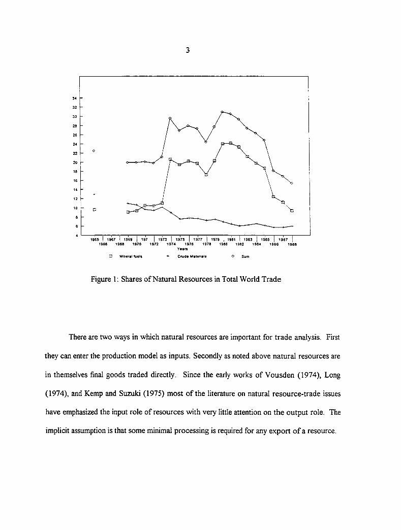
The answer to this question depends in part on the importance of natural resources in
trade between countries. Figure 1 shows the share of mineral oil and other natural resource
extractions in trade. Data for this graph was obtained from various issues of the Statistical
Yearbook series of the United Nations. It is clear from this that these account for an
appreciable portion of intercountry trade. Thus it appears that modem theories of
international trade that do not account for natural resource issues neglect a substantial
portion of trade.
3
Crude Materials
Figure 1; Shares of Natural Resources in Total World Trade
There are two ways in which natural resources are important for trade analysis. First
they can enter the production model as inputs. Secondly as noted above natural resources are
in themselves final goods traded directly. Since the early works of Vousden (1974), Long
(1974), and Kemp and Suzuki (1975) most of the literature on natural resource-trade issues
have emphasized the input role of resources with very little attention on the output role. The
implicit assumption is that some minimal processing is required for any export of a resource.
4
The motivation of this dissertation is based on two main observations. First it appears
that most of the theoretical and empirical analyses in international trade still rely heavily on
the static trade theorems outlined above. As much as these trade theorems are still of much
importance today, the conditions under which they hold true are very rare in reality. We will
investigate what happens when natural resource issues are considered and some of the
dynamic theorems that are needed. It may be that dynamic counterparts of the static
theorems exist in some situations. Though this work does not consider dynamic versions of
the static trade theorems, Kemp and Long (1984) provide a useful review of that aspect of
the literature.
The second observation that motivates this study is a general concern in
contemporary times about the relation between developing country debt burden and the rate
of depletion of natural resource stocks. There is believed to be the general tendency for
developing debtor nations to accelerate the extraction of their natural resource stocks in
order to pay off their debt and develop their economies. We will consider this problem and
see what happens when it is possible for the debtor nation to default.
Dissertation Organisation
This dissertation comprises of three separate but related papers preceded by a few
preliminary chapters. The first paper follows deals with the static issues encountered in
natural resource-trade models. These issues include the investigation of the conditions under

5
which static versions of the traditional trade theorems - Rybczynski, Stolper-Samuelson,
Heckscher-Ohlin and factor price equalization - hold. In the first paper we will concern
ourselves with the Rybczynski and Stolper-Samuelson theorems. The second paper of this
dissertation deals with the dynamic issues of natural resource-trade models. In that paper we
will consider production and trade patterns in the presence of natural resource extraction.
We generally assume that even if there is replenishment of the natural resource stock, it
generally is exhaustible.
As the third paper is somewhat different from the first two we did not give an
elaborate review of the literature associated with it in the general literature review above.
We have chosen to defer this so that an extensive review of the literature associated with the
third paper is included as part of that paper. The third paper deals with natural resource
extraction issues of particular interest to developing countries. Issues of interest include the
debt burden of these countries, creditor response to default risk and their implications for
natural resource extraction in those countries.
Each of the three papers includes a list of references cited in that paper and also a
concluding section summarizing the results of that paper. We conclude with a general
summary section for all the work embodied in the dissertation and a list of the references
cited in the chapters preceding the first paper.
6
THEORETICAL MODELS
Essentially, the process of modeling natural resource issues in trade involves either of
two approaches (Segerson, 1988):
(a) Adding natural resource stocks to a trade model as inputs or outputs or both OR
(b) Adding trade possibilities to a closed economy version of a natural resource model.
This process is not that simple, however, because there are some very important
differences between trade and resource models. Resources are usually modeled in dynamic
partial equilibrium frameworks emphasizing externalities in their analyses. Externalities result
because most resources are common property and there is little incentive to maintain a
complete set of property rights. Trade models on the other hand are usually static and for the
most part, ignore externalities; however, they are based on a more general equilibrium
approach (Antle and Howitt, 1988).
When the resource stock is regarded as an input in the production process we find
some similarities between this and the use of capital stocks in conventional models and so it
might seem that resource issues can be incorporated in trade models by simply treating them
as capital stocks. Just as the levels of capital stocks change over time so do the levels of
resource stocks and the d>Tiomics of resource stocks are at least as important as those of
capital stocks in the production model. However, some important differences are worth
noting. First, the resource stock is usually not (completely) owned by the firm and so it
usually does not internalize the effects of its actions on the common stock so that private
decisions may not be and usually are not socially optimal (Antle and Howitt, 1988).
Secondly whereas capital stocks change due to investment and depreciation, resource stocks
are augmented through biological or natural replenishment and depleted by use. So while the
augmentation of capital stocks is usually a choice variable and its depletion exogenous, the
reverse holds for resources (Segerson, 1988). Furthermore, the use of capital leads to
depletion in its quality, i.e. heterogeneity in its composition results while in the case of
7
resources changes in quantity rather than quality occur in most cases Kemp and Long (1984)
with few caveats.
There are many and varied treatments of the resource-trade linkage. Withagen (1985)
considers all models to be either partial equilibrium where they deal with the problem of
optimal exploitation of a natural resource stock when world market prices or demand
schedules are given or general equilibrium where demand is derived within the model. In this
section we first present the basic essentials common to all modeling approaches. Then it will
be appropriate to dilate on the various extensions that have occurred in the literature. The
problems encountered in this area of economics must necessarily be modeled in a dynamic
setting. The essential components of each modeling approach are the following;
1 • Capital and Variable Input Endowments:
This is common to all conventional trade and resource models and is an essential
feature here as well. Factor endovraients are bounded at a given time but there is always a
positive amount of every essential factor (available) at all times. The conventional H-0
model assumes we are interested in only two such variable inputs.
2. Natural Resource Endowments:
This is an addition to conventional trade models. There is a natural resource stock
which is bounded at a given time and possibly exhaustible so that we may have a zero
endowment level after some finite time. We distinguish three cases:
(a) Exhaustible and Norirenewablc: Kere the planning horizon involving the resource
allocation is finite, after which no resource stock is available.
(b) Renewable but Exhaustible: Some resources are renewable but exhaustible. The
dynamics is different from (a) but the period of resource use is finite as well because the
stock is used up over a finite horizon.
8
(c) Renewable and Nonexhaustible: Few resources come under an essentially infinite horizon
of existence in the sense that the usual depletion rate is highly superseded by the rate of
natural or artificial replenishment. The planning horizon for the resource stock is usually
infinite.
It is useful to note that whether the resource stock horizon is finite or infinite the
planning horizon for the whole optimization problem is usually infinite. So in the case of an
exhaustible resource, extraction occurs over a finite portion of the whole optimization
sequence.
Another issue of importance is whether or not the resource is extracted costlessly. As
we shall see this assumption has implications as to whether or not a period of incomplete
specialization intervenes between any two extremes of complete specialization.
3. Production Function:
All goods in the economy are produced nonjointly. Each production function exhibits
strict quasi-concavity and for virtually all cases, constant returns to scale (homogeneous of
degree one). N goods are produced each with m inputs some of which are natural resource
inputs, exhaustible or inexhaustible.
4. Capital Stock Dynamics:
In some cases the dynamics of capital use is explicitly outlined (Antle and Howitt,
1988). Capital changes due to investment and depreciation.
5. Resource Stock Dynamics:
This is a common feature in all models. The resource stock changes due to extraction
and replenishment. Corresponding to whether or not the type of resource is renewable we
have the following dynamics;
9
(a) Nonrenewable Resources
The changes in the resource stock are due only to the rates of extraction over time.
(b) Renewable Resources
The resource stock changes over time because of extraction as well as natural or artificial
replenishment.
(c) Replaceable Resources (Backstops)
When a country has more than one source of endowment for a particular use the extraction
of a resource stock may be replaced by the extraction of another.
6. Price/Market Structure or Trading Regime:
Most models assume that producers in a given country are in a perfectly competitive
market. Furthermore the small country assumption of exogenous prices is usually made. In
some cases (e.g. Kemp and Long, 1980b) the terms of trade is assumed to be constant as
well, while others allow it to grow at an exponential rate (e.g. Kemp and Long, 1982).
Usually, sticking as close as possible to the H-0 model it is assumed that only two countries
are involved in trade. Sometimes other market structures are assumed. Some studies deal
with a canei with the existence of a competitive fiinge. Others consider monopsony-
monopoly interactions.
7. Borrowing and Lending Possibilities:
One other aspect of variation involves international lending or borrowing possibilities.
1111 oi O iia a icai uii iiic iiaiuic ui iiic vjujcviivc aiiu iii lav i iiic wiiOic
modeling process. Kemp and Long (1984) note that the assumption of lending and
borrowing possibilities for a small country in which all inputs are natural resource variables
leads to a trivial solution. However, for the case where at least some inputs are not natural
resource variables this assumption leads to a nontrivial solution. At any rate assuming perfect
10
borrowing and lending on international markets means that maximization of the discounted
stream of output is necessary for the maximization of discounted utility (Segerson, 1988).
8. Preference Structure:
The standard assumption of identical preferences within a country is maintained. Also
it is usually assumed that preferences are identical across countries. However, in some
studies preferences are assumed to differ, or different rates of time preferences across
countries are assumed.
9. Objective Function:
The utility (or indirect utility) function of the representative agent of the economy is
the primary objective function, discounted by a positive and for the most part constant rate of
time preference. The optimization is done over an infinite horizon subject to the various
input and nonnegativity constraints. However, as stated earlier, when borrowing and lending
possibilities exist a necessary condition for utility maximization is the maximization of the
discounted stream of output. Output is discounted by the (not necessarily constant) rate of
intdroct pn/4 mpvim**7ptf/^r* pler> or*
Having spelt out the essential components of each of the models we now review in
more detail the basic structures involved. All the above components are important.
However, the models in literature are mainly discussed under three of them, viz.; production
structure, resource dynamics and market structure. Because treatment of the components is
not disjoint we shall consider the models under these three headings. Before we discuss them
it is useful at this stage to introduce notation that will be employed in the following sections.
Useful Notation
Define X/ , /" = l,.,w as the goods produced in country J.
11
Let V, K and E be the variable Ricardian (primary) input, capital input and Hotelling (natural
resource) input vectors respectively. Let P, W, R and S be the respective price vectors for
goods and Ricardian, capital and Hotelling factors. Because of the dynamic nature of such
models it is important to see the variables as sequences over time and sometimes it will be
necessary to compare sequences. In that case we would use the following notation:
Define y^'^) = (yKy^^^,.-) to be the sequence of the vector y fi-om time k to the end of the
planning horizon, which in most cases is infinite. When we write
y ( k ) > z ( k )
we mean that fi"om time k onwards, every time t element of y is greater than the
corresponding time t element of z for all t > k. The same holds for single variables so that
y (k)i> y (k)j
implies yi exceeds yj in value for all time beginning at time k.
Any vector y follows a given sequence from time zero onwards if undisturbed.
However, a disturbance at time k in the system, such as price or endowment changes, may
result in a different path for the vector. In order to distinguish the disturbed fi"om the
undisturbed time paths we denote the latter (undisturbed) as and the former (disturbed) N
sequence as so that
<y':)
means the disturbance in the system resulted in higher values than y for all time following
that disturbance.
We now proceed to review the models under the three main categories listed above.
Models Based On Differences In The Production Structure
Virtually all the models here are distinguished by the type of input vector involved.
12
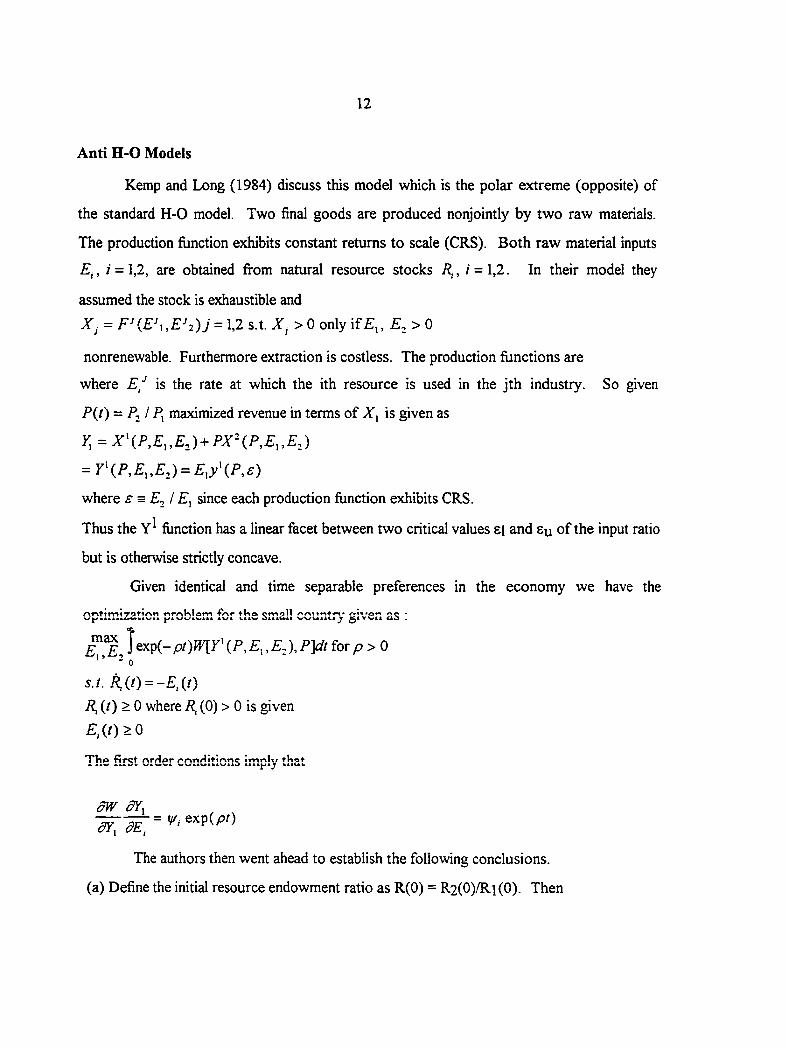
Anti H-0 Models
Kemp and Long (1984) discuss this model which is the polar extreme (opposite) of
the standard H-0 model. Two final goods are produced nonjointly by two raw materials.
The production fiinction exhibits constant returns to scale (CRS). Both raw material inputs
E., i = 1,2, are obtained fi-om natural resource stocks i = 1,2. In their model they
assumed the stock is exhaustible and
= F'iE'uE'z)] = 1,2 s.t. > 0 only if£,, £, > 0
nonrenewable. Furthermore extraction is costless. The production functions are
where E/ is the rate at which the ith resource is used in the jth industry. So given
P{t) = P^l maximized revenue in terms of is given as
Y, = X\P,E„E,) + PX\P,E,,E,)
= Y\P,E„E,) = Ey(P,s)
where s = E^ IE^ since each production function exhibits CRS.
Thus the function has a linear facet between two critical values el and Su of the input ratio
but is otherwise strictly concave.
Given identical and time separable preferences in the economy we have the
optimization problem for the small countr}' given as :
i " , I e x p ( - pt)W[y' Ez I for p > 0 ' ' - 0
s . t . R, i t ) = -£ , (! )
R i ( t ) > 0 w h e r e i ? , ( 0 ) > 0 i s g i v e n
£ , ( 0 > 0
nriiA -firct imnUr
The authors then went ahead to establish the following conclusions.
(a) Define the initial resource endowment ratio as R(0) = R2(0)/Ri(0). Then
13
R(0), constant if R(0) <s^
^(t)= j £(Oe(£^,fy)
[ R(0), constant if /?(0) > Sy
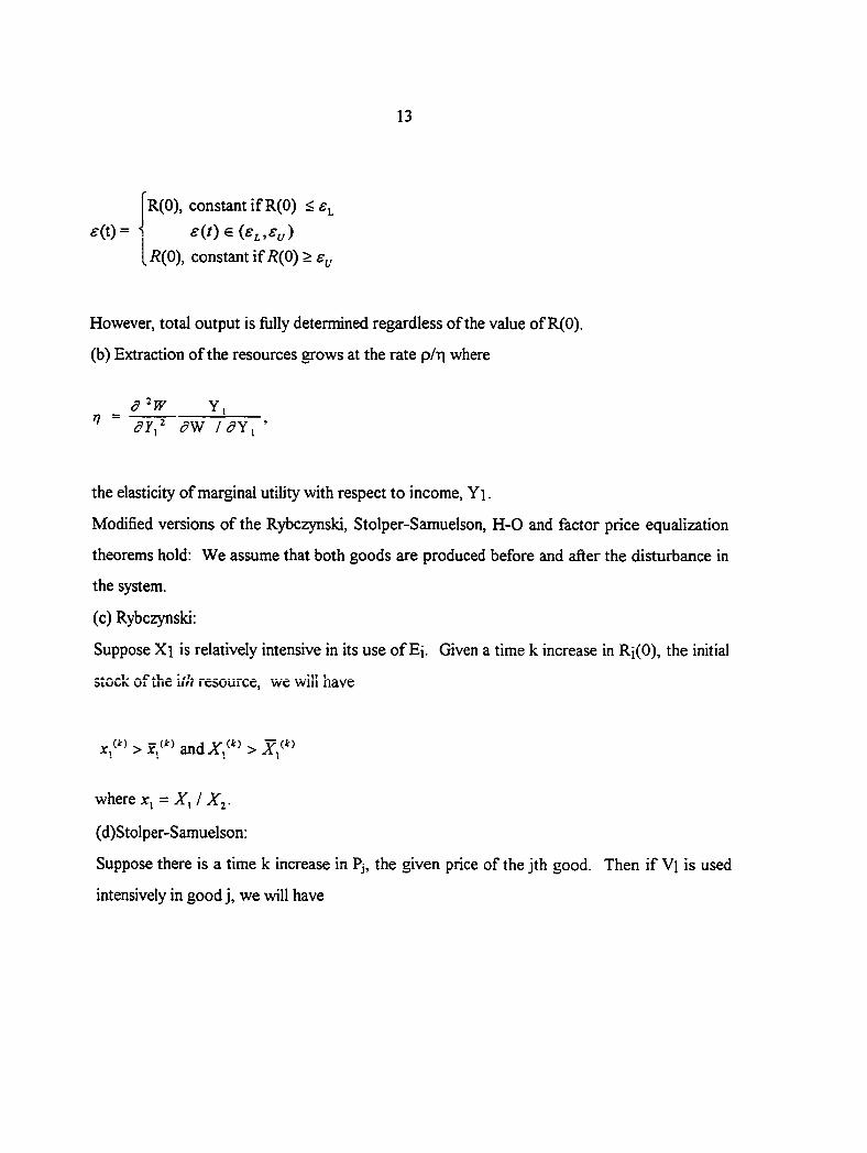
However, total output is fully determined regardless of the value of R(0).
(b) Extraction of the resources grows at the rate p/T| where
^ / ^ ? Y , '
the elasticity of marginal utility with respect to income, Y i.
Modified versions of the Rybczynski, Stolper-Samuelson, H-0 and factor price equalization
theorems hold: We assume that both goods are produced before and after the disturbance in
the system.
(c) Rybczynski:
Suppose Xi is relatively intensive in its use of Ei. Given a time k increase in Ri(0), the initial
stock of the iih Fcsourcc, wc will have
andA',/"'
where = XJ X^.
(d)Stolper-Samuelson:
Suppose there is a time k increase in Pj, the given price of the jth good. Then if V] is used
intensively in good j, we will have
14
where Xn = dX\ldW\ i=l,2 and a reduction in the marginal product of the other factor.
(e) Heckscher-Ohlin:
If preferences are strictly convex, homothetic and identical in each of the two free-
trading countries and if the rate of time preferences is everywhere the same and marginal
utility is of constant elasticity, then there is a trading equilibrium with constant terms of trade
and for as long as production continues, the country wWch is relatively well endowed with
the ith Hotelling factor will export the commodity which is relatively intensive in its use of
that factor.
Ono (1982) and others (e.g. Tawada, 1982) have shown that the strict sense of specialization
implied here is hinged on the assumption of the model such as zero or constant extraction
costs and that relaxation of that assumption will lead to various shades of incomplete
specialization.
(f) Factor Price Equalization:
If all of the above conditions for the H-0 theory hold then there exists an equilibrium
terms of trade and an associated cone of diversification which is the same for all points of
time at which production takes place. Furthermore in each country the extraction ratio s(t) is
constant being equal to the initial endowment ratio. Then if and only if the extraction vectors
of the two countries lie in the common cone of diversification, the marginal product of each
resource will be the same in both countries.
Hybrid Models
In these models (e.g. Kemp and Long, 1984, 1982, 1980b, 1980d and 1978) we have
two inputs, one Hotelling and one Ricardian in a CRS production function each country
15
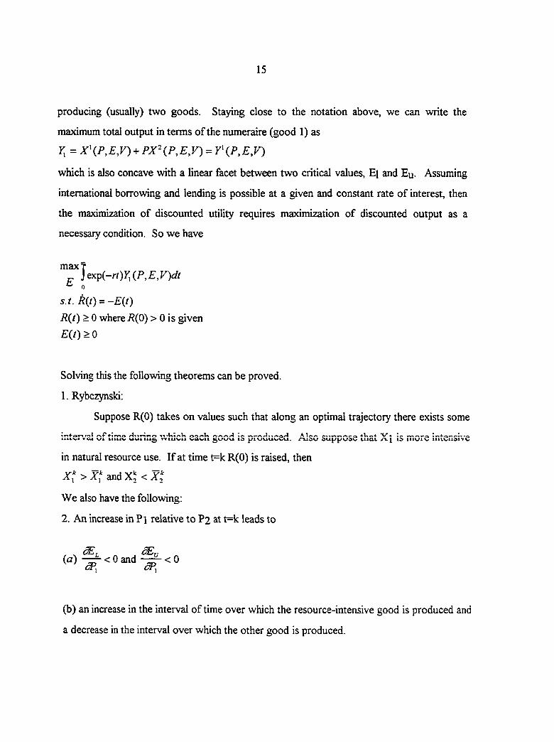
producing (usually) two goods. Staying close to the notation above, we can write the
maximum total output in terms of the numeraire (good 1) as
y; = x\p,Ey)+PX\p,E,v) = Y\P,E,V)
which is also concave with a linear facet between two critical values, E] and Eu- Assuming
international borrowing and lending is possible at a given and constant rate of interest, then
the maximization of discounted utility requires maximization of discounted output as a
necessary condition. So we have
max? Jexp(-r/)?;(P,£,Fy/
^ 0 s.t . R(t) = -E{t)
R{t) > 0 where i?(0) > 0 is given
E(0>0
Solving this the following theorems can be proved.
1. Rybczynski;
Suppose R(0) takes on values such that along an optimal trajectory there exists some
iAi«,w voa \ji. vAuiiii^ wiiAvii wawii Id rxidu mat yv| id iiioiv iiitwiidivc
in natural resource use. If at time t=k R(0) is raised, then
Xf > X,' and < X.
We also have the following:
2. An increase in Pi relative to P2 at t=k leads to
( a ) — < O a n d — < 0
(b) an increase in the interval of time over which the resource-intensive good is produced and
a decrease in the interval over which the other good is produced.
16
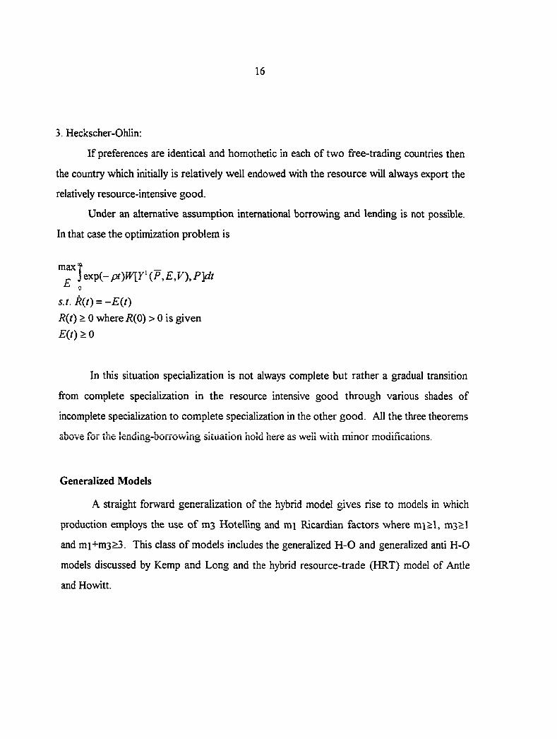
3. Heckscher-Ohlin;
If preferences are identical and homothetic in each of two free-trading countries then
the country which initially is relatively well endowed with the resource will always export the
relatively resource-intensive good.
Under an alternative assumption international borrowing and lending is not possible.
In that case the optimization problem is
max? _ „ ]tx:pi-pt)W[riP,E,V),P]dt ^ 0
s.t . Rit) = -Eii)
R(t) > 0 where R(P) > 0 is given
£(/) > 0
In this situation specialization is not always complete but rather a gradual transition
from complete specialization in the resource intensive good through various shades of
incomplete specialization to complete specialization in the other good. All the three theorems
above for the Icnuing-borrowing Situation hold here as well with minor modifications.
Generalized Models
A straight forward generalization of the hybrid model gives rise to models in which
production employs the use of m3 Hotelling and m] Ricardian factors where mi>l, m3>l
and mi+m3>3. This class of models includes the generalized H-0 and generalized ami H-0
models discussed by Kemp and Long and the hybrid resource-trade (HRT) model of Antle
and Howitt.
17
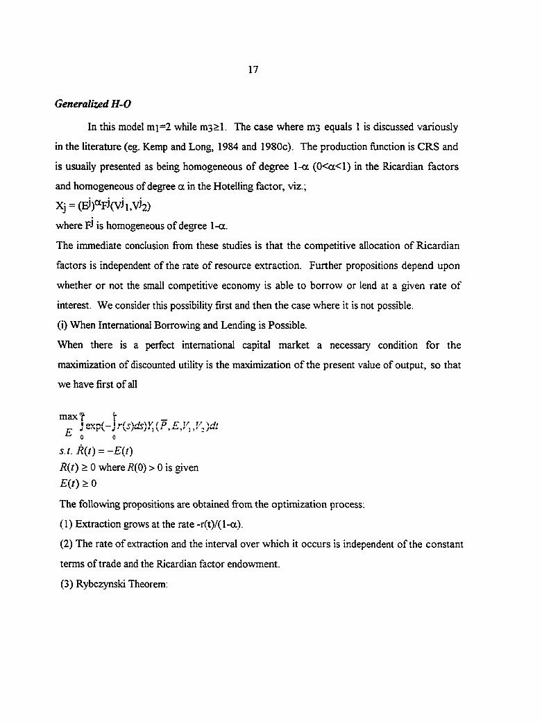
Generalized H-0
In this model mi=2 while m3>l. The case where ms equals 1 is discussed variously
in the literature (eg. Kemp and Long, 1984 and 1980c). The production function is CRS and
is usually presented as being homogeneous of degree 1-a (0<a<l) in the Ricardian factors
and homogeneous of degree a in the Hotelling factor, viz.;
Xj = (Ei)«Fj(V)i,vj2)
where F-l is homogeneous of degree 1-a.
The immediate conclusion fi-om these studies is that the competitive allocation of Ricardian
factors is independent of the rate of resource extraction. Further propositions depend upon
whether or not the small competitive economy is able to borrow or lend at a given rate of
interest. We consider this possibility first and then the case where it is not possible.
(i) When International Borrowing and Lending is Possible.
When there is a perfect international capital market a necessary condition for the
maximization of discounted utility is the maximization of the present value of output, so that
we have first of all
maxf t _ \ oyrT^(-\ ^\r1c-\V ( P (Tl/ • ^ 0 0
s.t . R{t) = -E{t)
Rit) > 0 where i?(0) > 0 is given
E{t) > 0
The following propositions are obtained firom the optimization process:
(1) Extraction grows at the rate -r(t)/(l-a).
(2) The rate of extraction and the interval over which it occurs is independent of the constant
terms of trade and the Ricardian factor endovraient.
(3) Rybczynski Theorem:
18
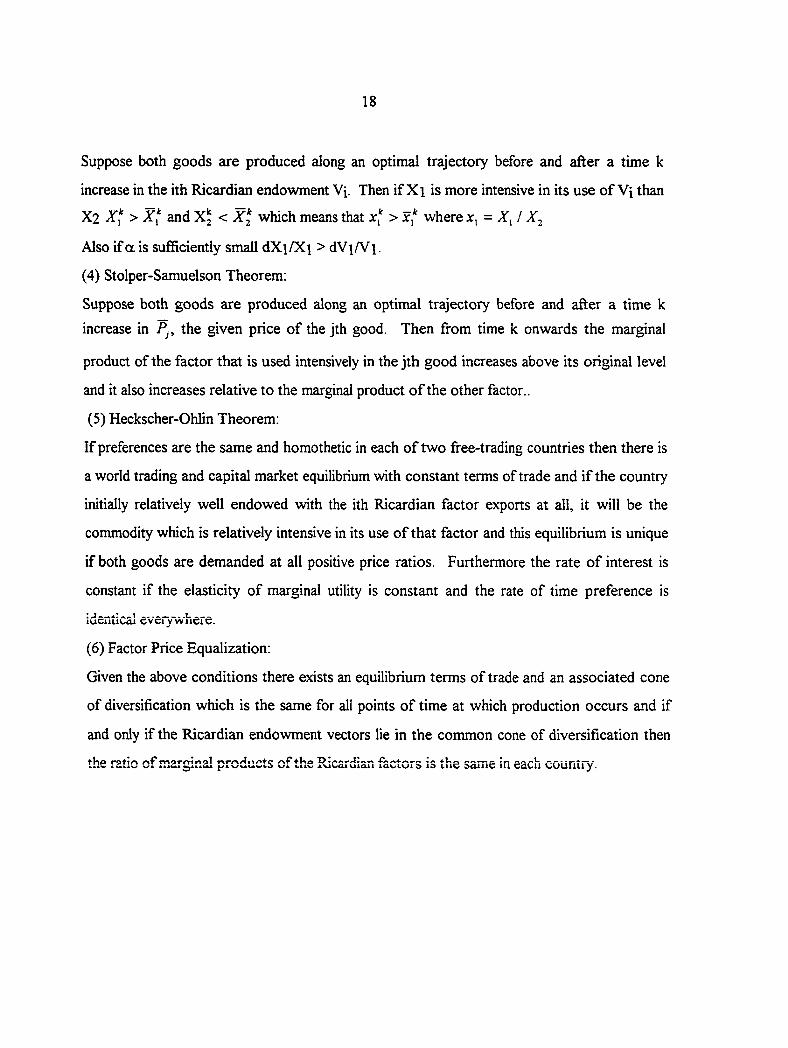
Suppose both goods are produced along an optimal trajectory before and after a time k
increase in the ith Ricardian endowment Vi. Then if Xi is more intensive in its use of Vi than
X2 A'f > and Xj < which means that xf > where x^ = XJ X^
Also if a is sufficiently small dXi/Xi > dV\fV\.
(4) Stolper-Samuelson Theorem:
Suppose both goods are produced along an optimal trajectory before and after a time k
increase in P^, the given price of the jth good. Then from time k onwards the marginal
product of the factor that is used intensively in the jth good increases above its original level
and it also increases relative to the marginal product of the other factor..
(5) Heckscher-Ohlin Theorem;
If preferences are the same and homothetic in each of two free-trading countries then there is
a world trading and capital market equilibrium with constant terms of trade and if the country
initially relatively well endowed with the ith Ricardian factor exports at all, it will be the
commodity which is relatively intensive in its use of that factor and this equilibrium is unique
if both goods are demanded at all positive price ratios. Furthermore the rate of interest is
constant if the elasticity of marginal utility is constant and the rate of time preference is
identical everywhere.
(6) Factor Price Equalization:
Given the above conditions there exists an equilibrium terms of trade and an associated cone
of diversification which is the same for all points of time at which production occurs and if
and only if the Ricardian endoAvment vectors lie in the common cone of diversification then
the ratio of marginal products of the Ricardian factors is the same in each country.
19
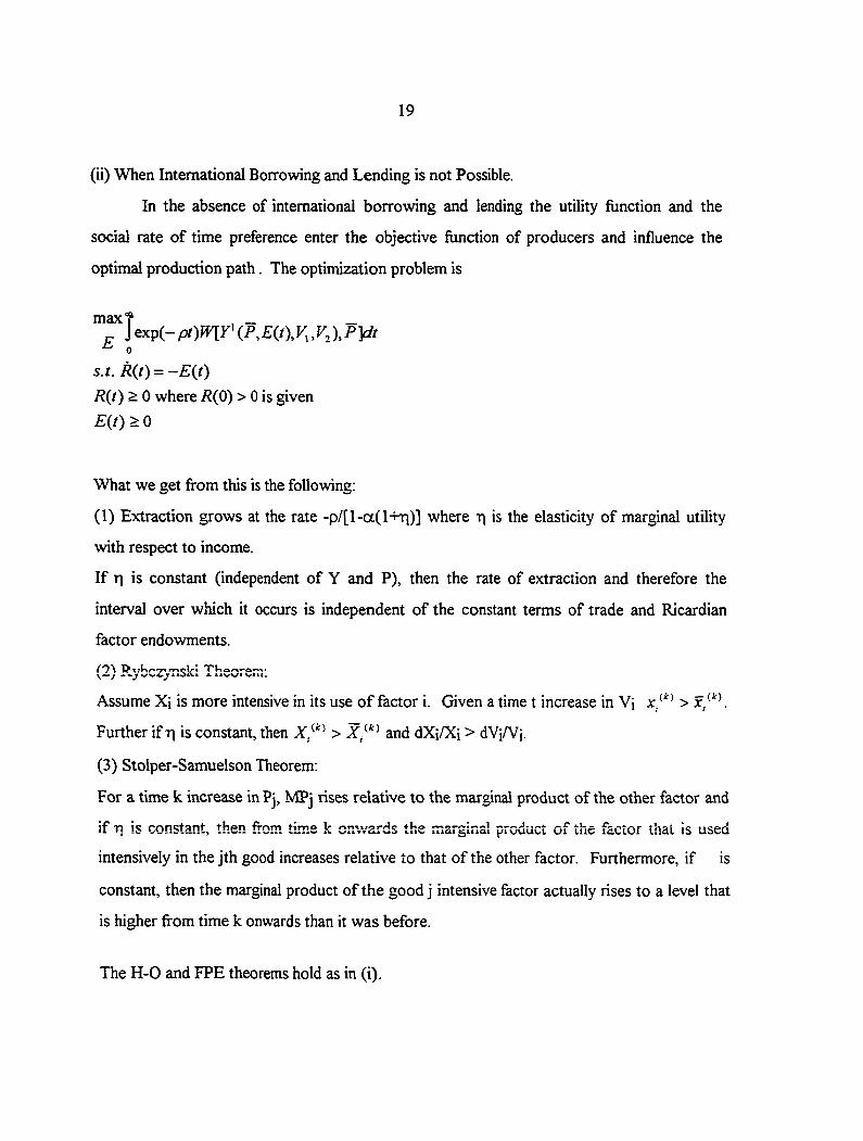
(ii) When International Borrowing and Lending is not Possible.
In the absence of international borrowing and lending the utility function and the
social rate of time preference enter the objective function of producers and influence the
optimal production path. The optimization problem is
maxf _ _ Jexp(-p/Mr'(P,£(/),F„F,),/>>//
^ 0 s.t . Kit) = -E{t)
R{t) > 0 where R(Q) > 0 is given
E{t) > 0
What we get fi^om this is the following:
(1) Extraction grows at the rate -p/[l-a(l-hi)] where ti is the elasticity of marginal utility
with respect to income.
If r\ is constant (independent of Y and P), then the rate of extraction and therefore the
interval over which it occurs is independent of the constant terms of trade and Ricardian
factor endowments.
(2) R.ybcz>T.ski Theorem;
Assume Xi is more intensive in its use of factor i. Given a time t increase in Vi
Further if t\ is constant, then and dXi/Xi > dViA^j.
(3) Stolper-Samuelson Theorem;
For a time k increase in Pj, MPj rises relative to the marginal product of the other factor and
if n. is constant, then from time k onwards the marginal product of the factor that is used
intensively in the jth good increases relative to that of the other factor. Furthermore, if is
constant, then the marginal product of the good j intensive factor actually rises to a level that
is higher from time k onwards than it was before.
The H-0 and FPE theorems hold as in (i).

20
Generalized Anti H-0
For this class of models (eg. Kemp and Long, 1984) we have mi>l while m3=2.
Each good Xj, j=l,...,n is produced as
where \\i and ^ are homogeneous of degree one.
Kemp and Long report that all the theorems for the anti H-0 models hold here as well when
generalized.
Hybrid Resource-Trade (HRT) Models
In their article Antle and Howitt (1988) develop "hybrid" resource-trade (HRT)
models to quantify resource-trade linkages. Realizing the central role of the production
process in this linkage they used a lucid four-step procedure in their presentation;
1. Derivation of the linkage between agricultural production and natural resources
2. Derivation of the linkage between agricultural production and trade.
3. Joining the two linkages to get HRT models
4. Use of the HRT models to analyze policy issues.
x i ic uadiu cddci iLio id u i p iuuuci iu i i l i iuuc i a ic a5 lOi iOw^.
Production function:
qit = fi(sit,zit,rit) i = l,...,I
where sit, zit are vectors of allocated resource stocks and purchased capital and rjt is a vector
of vsrisbls factor inputs
Capital stock dynamics:
zit+1 - zit = -5zit + vit
21
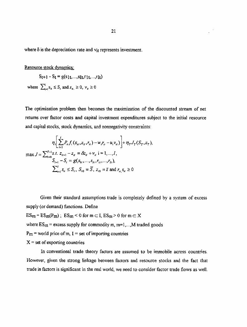
where 5 is the depreciation rate and vit represents investment.
Resource stock dynamics:
St+1 - St = g(sit,...,sit.rit,...,rit)
where ^^.,3;, < S, ands^, > 0, > 0
The optimization problem then becomes the maximization of the discounted stream of net
returns over factor costs and capital investment expenditures subject to the initial resource
and capital stocks, stock dynamics, and nonnegativity constraints:
Given their standard assumptions trade is completely defined by a system of excess
supply (or demand) functions. Define
ESm = ESm(Pm); ESm < 0 for m c I, ESm > 0 for m c X
where ESm - excess supply for commodity m, m=l,...,M traded goods
Pm = world price of m, I = set of importing countries
X = set of exporting countries
In conventional trade theory factors are assumed to be immobile across countries.
However, given the strong linkage between factors and resource stocks and the fact that
trade in factors is significant in the real world, we need to consider factor trade flows as well.
max J= = &„ +v„ i = 1,.. . , / , •^f=0
22
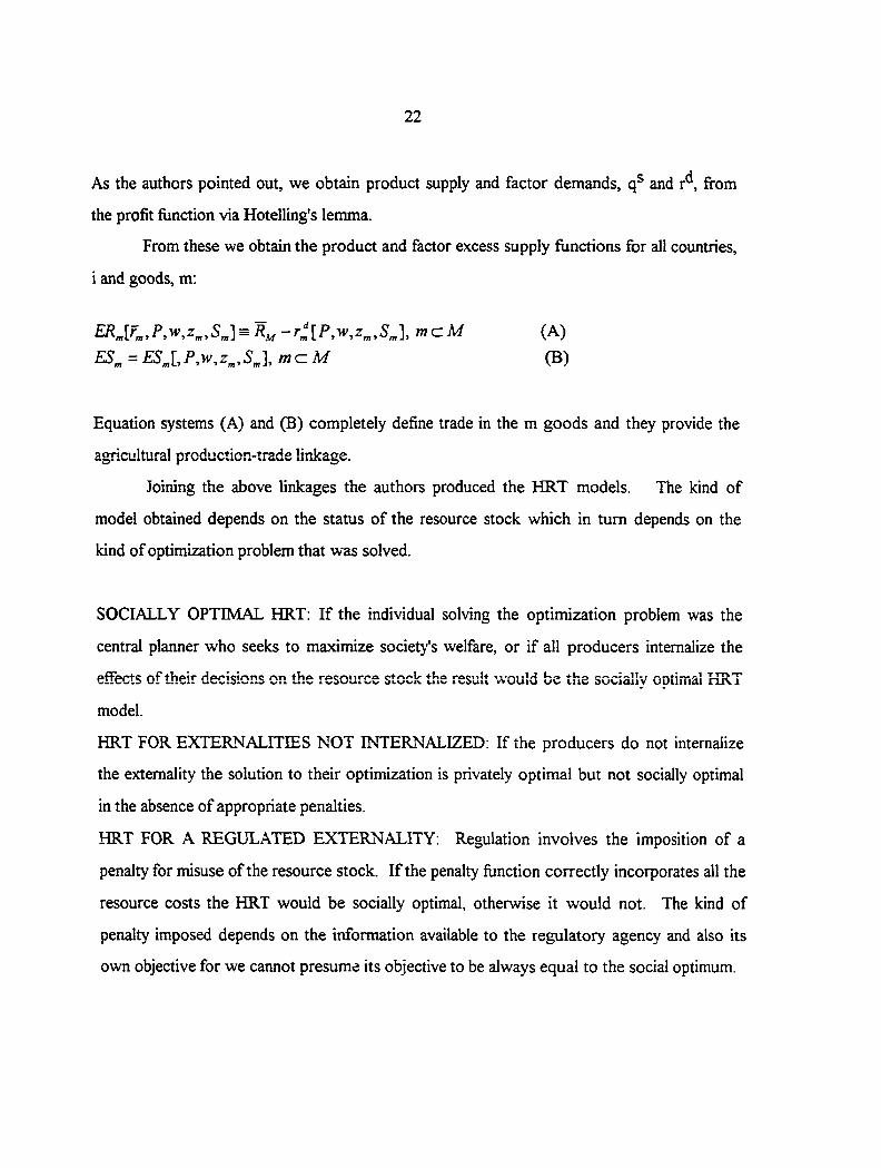
As the authors pointed out, we obtain product supply and factor demands, and r^, from
the profit function via Hoteiling's lemma.
From these we obtain the product and factor excess supply functions for all countries,
i and goods, m:
= mczM (A)
ES„ = ESJ,P,w,z„,S„l w c M (B)
Equation systems (A) and (B) completely define trade in the m goods and they provide the
agricultural production-trade linkage.
Joining the above linkages the authors produced the HRT models. The kind of
model obtained depends on the status of the resource stock which in turn depends on the
kind of optimization problem that was solved.
SOCIALLY OPTIMAL HRT; If the individual solving the optimization problem was the
central planner who seeks to maximize society's welfare, or if all producers internalize the
effects of their decisions on the resource stock the result would be the socially optimal HRT
model.
HRT FOR EXTERNALITIES NOT INTERNALIZED: If the producers do not internalize
the externality the solution to their optimization is privately optimal but not socially optimal
in the absence of appropriate penalties.
HRT FOR A REGULATED EXTERNALITY; Regulation involves the imposition of a
penalty for misuse of the resource stock. If the penalty function correctly incorporates all the
resource costs the HRT would be socially optimal, otherwise it would not. The kind of
penalty imposed depends on the information available to the regulatory agency and also its
own objective for we cannot presume its objective to be always equal to the social optimum.
23
Models Based On Differences In Resource Dynamics
The nature of resource dynamics is a very important distinguishing feature among the
various models. Virtually all the models we have considered so far assume that the resource
stock is nonrenewable and non-replaceable (eg. Kemp and Long, 1980b and 1980c). In this
section we note that when that assumption is relaxed the optimization problem becomes more
complex and the possibility of non-trivial steady states in which various rates of extraction are
matched by rates of renewal (or replacement) becomes more apparent (Kemp and Long,
1984). Our attention here is directed at showing the changes that occur in the optimization
problems due to varying assumptions of resource dynamics rather than showing which, if any,
of the standard theorems are violated.
Nonrenewable And Non-Replaceable Resources
This has been the underlying assumption of resource dynamics in most of the models
discussed above. For any resource stock i=l,...,m the rate of extraction depends only on the
rates of use of the resources in the n goods.
Renewable Resources
When the resource is renewable the time rate of change of the stock depends not only
on the rate of extraction but also on the rate at which it is being renewed either naturally or
artificially or both. The rate of renewal or growth is usually posited as a function g() of the
stock.
It is easily conceivable that an economy may have more than one natural resource
endowment serving similar purposes so that in a sense the various resource endowments are
substitutes. Kemp and Long (1984) consider the case where energy can be obtained from oil
or from solar sources. In this case the optimization problem is divided into segments, mostly
finite . For each segment one or more resource types Rj are extracted for use in production.
24
This is followed by another segment having a different combination of resource types. Thus
for any period of time te[Tic,Tk+l] suppose that the complete form of the objective function
is given as Y().
Replaceable Resources [Backstops]
For the period t6[Tk+l,Tk+2] and so on different combinations of resource
endowments are called upon for production. The time intervals are themselves choice
variables of the whole optimization problem, chosen to maximize the whole discounted
stream of the objective function (maximand) for the infinite planning horizon.
Differences In Price/Market Structure Or Trading Regime
For most of the models described above the authors assumed the conditions of perfect
competition to prevail. However, it is conceivable and in fact a reality that some resources
such as fossil fuels are not traded in such markets. In the literature attention has been drawn
to other market structures and the most firequentiy used are caneis and monopoly-
monopsony relations. The major motivation for noncompetitive market structures is the
uneven distribution of resource deposits across the globe. When noncompetitive market
structures are considered the result is usually dependent upon whether it is price or quantity
that is the strategic choice variable of concern. We proceed to describe briefly the
implications of such market structures, with most reference to price setting behaviors.
25
Cartels
Studies on this type of market structure assume that the cartel is operating in the
midst of a competitive fringe. The nature of the optimization problem of a country therefore
depends upon the actions of the cartel and whether it is a member or not. The approach to
analysis then involves a derivation of the cartel's (pricing) behavior and the implied behavior
of the competitive fnnge. Since in most cases the competitive fringe takes the price set by
the cartel as given we have a Stackelberg rather than a Nash-Coumot setting.
Newbery (1981) analyzed the world oil market with the assumption that OPEC acts
as a cartel facing a competitive fringe. His concern was with the issue of dynamic
inconsistency. He argued that there is a high incentive for the cartel to deviate from its
previously announced price path in the case of nonbinding contracts because its rational
expectations equilibrium would be the price path which maximizes its present value
discounted profit at each successive date rather than the initial date only. He shows,
however, that the Nash-Coumot equilibrium is dynamically consistent and is the best
approximation to the Stackelberg outcome. He uses a graphical approach (as opposed to
dynamic programming techniques) to derive the price path of the cartel, arguing that dynamic
programming techniques usually do not expose solutions which are dynamically inconsistent.
There are essentially two possible phases
(a) A competitive phase during which the fringe operates and
(b) A monopolistic phase during which the fringe does not operate
26
Whether one or both phases occur and the order in which they do depends on the
assumptions of the model
Kemp and Long (1984) also consider binding and nonbinding contracts for cartels and show
that dynamic inconsistency is highly probable for nonbinding contracts.
Monopoly-Monopsony Interactions
In a series of papers some authors (e.g. Chiarella, 1980, and Kemp and Long, 1980e
and 1980f) considered the problem of trade in natural resource deposits when one country or
group of countries is resource-rich while the other is resource-poor. In the extreme case we
may have a monopoly created by the resource-rich and/or monopsony by the resource-poor.
The implications of the market structure depend on whether or not the monopoly can utilize
its resource deposits domestically, i.e., what resource disposal options are open to it. It also
depends upon the leverage of the monopsony in terms of the power it commands in trade
with the resource monopoly in other goods. Most authors are of the opinion that the
monopsony can exploit the monopoly if the latter has no other use for the resource.
However, if the monopoly can utilize the resource domestically it is less susceptible to
exploitation.
The case of a monopoly and monopsony in the presence of a cartel is also considered
in the literature (Kemp and Suzuki, 1975).
27
EMPIRICAL MODELS
Most of the attempts at modeling resource-trade linkages have been theoretical.
Empirical models are difficult to estimate and have been largely avoided. The importance of
empirical tests to theoretical models can be appreciated when one recalls the Leontief
paradox, wluch is not without criticisms, however. Empirical tests for the above models are
needed to help improve their applicability to real world conditions.
Segerson (1988) suggests that the various kinds of environmental externalities should
be taxonomized to streamline empirical evaluations. The key problem remaining is still the
valuation of the externality. Abbott and Haley (1988) suggest two alternative approaches at
estimation:
(a) Linear Programming Economywide models as popularized in the development literature
(b) Computable General Equilibrium models though in the past these have hardly ever been
used to incorporate externalities.
Theoretically we expect environmental control costs to lead to increased
specialization in the production of polluting products in countries with less stringent
environmental policies and the reverse to hold for countries with more strict policies
(McGuire (1982), Pethig (1976) and Siebert (1977)). However, some studies have cast
doubt on the significance of this seemingly plausible notion . Some interesting studies by
Pearson (1985) and Walter (1982) using the location of industry approach also find that
evidence is lacking in support of the hypotheses that 'dirty' industries move out of the stricter
28
countries (industrial-flight hypothesis) to the less strict countries (pollution-haven
hypothesis). Following Learner (1984) and others (e.g. Bowen and Learner, 1987) the
objective of Tobey (1990) was to use a Heckscher-Ohlin-Vanek (HOV) model to perform an
empirical test on this notion.
Tobey considered the effects of domestic envirorunental policies on the patterns of
world trade. He tested empirically the hypothesis that the degree of environmental policy
restrictions have no effect on the comparative advantage of countries as reflected by the
patterns of world trade. This was a relatively simple model, using cross-sectional 1975 data
for 23 countries. The HOV model fitted in the usual way is;
Nj = Vjp + pj
He included a dummy variable (Dj) representing stringency of pollution control measures in a
country
Nj = VjP + Djpk+1 + Mj
and fitted the above system by ordinary least squares (OLS).
Nj is a Ixn vector of net exports of n commodities by country j, Vj is a Ixk vector of (k)
resource endowments of country j, P is a kxn matrix of parameters for country j, Pk+1 is a
Ixn vector of dummy variable parameters and |aj is the disturbance term. Though he did not
make any explicit assumption regarding the disturbance term the use of OLS regression
techniques presumes that it has a spherical distribution and in particular
" MVN[0,c7-I]
29
which is to say the disturbances are distributed multivariate normal with zero mean vector
and variance matrix a^I. This is needed to ensure unbiasedness and other nice properties of
the parameter estimates.
Data on Dj was obtained from a 1976 UNCTAD survey by Walter and Ugelow (1979). He
divided the n commodities into five groups and run separate regressions for each of them. He
concluded that because bk+l, the estimated value of Pk+l is not statistically significant in any
case environmental policy stringency has not affected trade patterns appreciably.
To give fiirther proof of his findings Tobey used a second procedure, an omitted
variable test. He considers the bias in the regression residuals that is caused by omitting Dj
from the equation system. His findings confirm the previous conclusion that environmental
policy stringency has no appreciable effect on trade patterns. He then extends the HOV
model to account for non-homothetic preferences and then scale economies and product
differentiation. Finally a fixed effects empirical test also leads to the conclusion that policy
stringency has no appreciable effect on patterns of trade.
Bowen (1983) considered the impact of changes in international resource distribution
on U.S. comparative advantage. Using regression techniques and graphical analyses he
studies capital, skilled, semiskilled and unskilled labor and arable land distribution patterns
vis-a-vis comparative advantage over five years. He concludes that factor distribution is an
important determinant of U.S. comparative advantage. He used a similar empirical model as
Tobey except that he was not interested in environmental policy impacts and so did not
30
include a policy stringency term. However, performing the analysis over five years represents
an improvement over Tobey since it is difficult to say anything about trade patterns from a
one year result. At any rate there appears to be considerable problems with both models.
Firstly it seems that 'simplistic' OLS regression of net exports on factor endowments
may not account for most of the major determinants of trade patterns. It is conceivable that
patterns of trade have been influenced by political factors and other shock terms that are not
very far fetched. Thus neglection of these leads to spurious results. In Tobey one also sees
the problem of how to group countries for policy stringency. Since the grouping was done
on the basis of level of development the total effects of policy stringency was masked. Some
other grouping could lead to different resuhs. However, these are rare attempts and
represent a considerable achievement. Notable areas of improvement needed in the empirical
literature are:
1. Choice of relevant variables.
2. Nature of the dependent variable.
3. Functional form to be estimated.
4. Choice of empirical technique.
5. The most appropriate way to represent the environmental policy component
31
PAPER 1:
STATIC TRADE THEOREMS IN THE GENERALIZED H-0 MODEL
32
1: INTRODUCTION
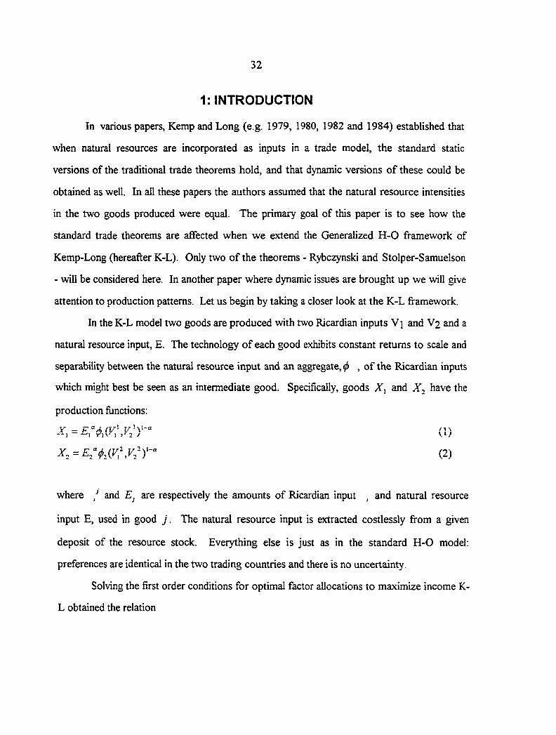
In various papers, Kemp and Long (e.g. 1979, 1980, 1982 and 1984) established that
when natural resources are incorporated as inputs in a trade model, the standard static
versions of the traditional trade theorems hold, and that dynamic versions of these could be
obtained as well. In all these papers the authors assumed that the natural resource intensities
in the two goods produced were equal. The primary goal of this paper is to see how the
standard trade theorems are affected when we extend the Generalized H-0 framework of
Kemp-Long (hereafter K-L). Only two of the theorems - Rybczynski and Stolper-Samuelson
- will be considered here. In another paper where dynamic issues are brought up we will give
attention to production patterns. Let us begin by taking a closer look at the K-L framework.
In the K-L model two goods are produced v^ath two Ricardian inputs V \ and V2 and a
natural resource input, E. The technology of each good exhibits constant returns to scale and
separability between the natural resource input and an aggregate, <f) , of the Ricardian inputs
which might best be seen as an intermediate good. Specifically, goods X, and have the
production functions;
(1)
(2)
where / and Ej are respectively the amounts of Ricardian input , and natural resource
input E, used in good j. The natural resource input is extracted costlessly from a given
deposit of the resource stock. Everything else is just as in the standard H-0 model:
preferences are identical in the two trading countries and there is no uncertainty.
Solving the first order conditions for optimal factor allocations to maximize income K-
L obtained the relation
33
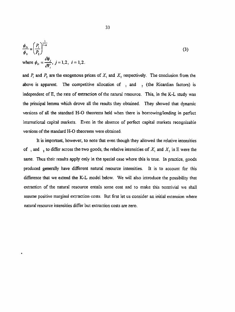
^py~ I-a (3)
where = —, j = 1,2, i = 1,2.
and P, and are the exogenous prices of AT, and X, respectively. The conclusion from the
above is apparent. The competitive allocation of , and , (the Ricardian factors) is
independent of E, the rate of extraction of the natural resource. This, in the K-L study was
the principal lemma which drove all the results they obtained. They showed that dynamic
versions of all the standard H-O theorems held when there is borrowing/lending in perfect
international capital markets. Even in the absence of perfect capital markets recognizable
versions of the standard H-0 theorems were obtained.
It is important, however, to note that even though they allowed the relative intensities
of , and 2 to differ across the two goods, the relative intensities of A', and in E were the
same. Thus their results apply only in the special case where this is true. In practice, goods
produced generally have different natural resource intensities. It is to account for this
difference that we extend the K-L model below. We will also introduce the possibility that
extraction of the natural resource entails some cost and to make this nontrivial we shall
assume positive marginal extraction costs. But first let us consider an initial extension where
natural resource intensities differ but extraction costs are zero.
34
2: THE GENERALIZED H-0 MODEL WHEN NATURAL RESOURCE
Everything else is the same as in K-L. We obtain the K-L model as a special case by setting
a = p. In the present model we shall assume that international borrowing and lending is
possible in perfect capital markets so that a necessary condition for the maximization of
discounted utility is the maximization of the present value of the income stream (Segerson,
1988). Thus we can solve the optimization problem in two stages:
Stage I: Given the level of E for a specific time, optimize the allocation of the three factors
among the two goods - a static problem.
Stage II: Given the optimum allocation of factors (and hence optimized national revenue)
derive the time path of E that maximizes the discounted stream of income - a dynamic
problem.
As mentioned earlier our focus in this paper is on the Stage I problem, to which we now turn.
At each point in time we have a fixed stock of each of two Ricardian factors.
Assuming a given level of natural resource extraction our static problem is to choose the
allocation of the three factors that maximizes total income at a point in time. For notational
convenience let the two Ricardian factors be labor, L, and capital, K so that
INTENSITIES DIFFER
Our initial extension of the K-L model gives us:
(4)
(5)
X, = j = 1,2, a, = a, a, =0. (6)
Our static problem then becomes more formally.
(7)
35
The Lagrangian for this problem can be defined as;
1 = + k,{E-E,-E.]+?. . [K-K,-K.- \ + k^[L-L,-L^] (8)
where A,., / = 1,2,3 are multipliers.
The first order conditions for an interior solution are:
=0 (9)
E.:PP^E.^'<j>,^-^-X,=0 (10)
= 0 (11)
Z.: (1 -P)P.E.^(!>;''- ;i3 = 0 (12)
/:,:(l-a)/^£,V,-V„-^3=0 (13)
/:,:(l-)ff)P,£/<i3-V2. = 0 (14)
where o,, = —- and = —- .
It is readily apparent from the above system that the usual result for a competitive
allocation of factors is realized - for each factor, marginal products across final goods are
equalized:
^ A V-" 11
\Ey J = PP
f , <P2
\^2 / (15)
(l-a)P. , A . V r 1 • A. \Y2
^21 (16)
(l-a)P, \4'\^
'l>^2=i^-P)P2 f TT E^
\^2'^ ^22 (17)
36
It is the ratio of marginal factor products in the intermediate goods, —, that reflects the h
competitive allocation of Ricardian factors. An implied result from the above is that
— = — as also expected. Let us define this as 9 11 12
= (18) Vn <P\2
Solving for n from (16) one obtains
09) (l-/7)a(«>,/(»,)
The interpretation of this is that the allocation of Ricardian factors is dependent upon the rate ( E / £ , )
of natural resource use in the two goods except in the extreme case where — i<t>\ I ^2)
is a constant. Recall that we may solve the above system to obtain £, = £,(£, .K', L, fj, A),
KJ = K.(E,K,L,P^,P2), and L^ = L.{E,K,L,P^,P^) generally nonlinear functions in their
arguments. Thus we may unally conclude in contrast to the K-L result that:
Lemma 1:
When the natural resource intensities differ across the two goods the competitive allocations
of the Ricardian factors is a function of the rate of extraction, E, of the natural resource stock.
As we turn to our analysis of the Rybczynski and Stolper-Samuelson theorems it
would be much easier and more insightfiil to use a dual approach to the above problem.
Furthermore to make the analysis more tractable we shall impose more structure on the
technology. Specifically we assume from here on that the intermediate goods and are
also of Cobb Douglas constant returns form in the labor and capital inputs:
37
I -1
(j, , = L.'K;-", a €(0,l), b €(0,1). (20)
Let be the wage rate for labor, R the rental rate for capital and Pe the price of the natural
resource input. Then corresponding to the above production technology the cost function of
the first good, will be;
C, = (21)
where = {a''[a(l-a)]''^''"^[(l-a)(l-a)y'"''^'"''^} '
Similarly the cost function for the second good is given as
a = (22)
where = {/? ^ [6(1 - p )]'^'-^^[(l - &)(1 - p
Thus we know that
•^ = 1 = ,23) oX^
^ = P = ( 2 4 )
Hence by Shepherd's lemma the input allocations are given as
IT oY] (25)
RPY (26)
a(l-a)Z, i—^ (27)
38
_b{\-P)PX,
W
^ a)X, ' R
^ _ {\-b){\-P)PX,
' R
(28)
(29)
(30)
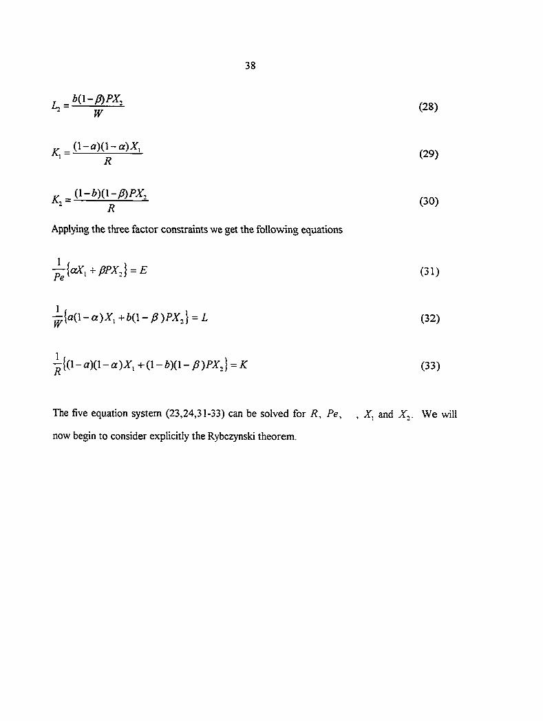
Applying the three factor constraints we get the following equations
y^\cOt,*l3PX,\ = E (31)
^ { a ( , l - a ) X , + b { \ - P ) P X , ] = L (32)
i{(I - aXl - a ) A-, + (I - d)(l - A I = ^ (33)
The five equation system (23,24,31-33) can be solved for R, Pe, , X, and X^. We will
now begin to consider explicitly the Rybczynski theorem.

39
3: THE RYBCZYNSKI THEOREM
There are two main versions of the Rybczynski theorem that we will consider. The
standard (or strong) version states that if commodity prices are held fixed, an increase in the
endowment of one factor causes a more than proportionate increase in the output of the
commodity which uses that factor relatively intensively and an absolute decline in the output
of the other commodity. A weaker version would imply that the output of the good more
intensive in that factor would rise relative to that of the other good. For the moment let us
consider the standard version.
3.1: The Standard Version of Rybczynski
Forgetting about magnitudes of output and factor changes, a variant of the standard
version, which we would call the moderate version, implies that an increase in the endowment
of a factor should lead to an increase in the output of the good intensive in that factor and a
decline in the output of the other good, granted that commodity prices are held fixed. This
moderate version is what we will be mainly concerned with in this section because it is easier
to characterize since we deal only with signs and not magnitudes of derivatives. If we are able
to show that this version does not hold under certain scenarios, then we know the standard
version does not hold under those conditions. However, if the moderate version holds it does
not imply that the standard version does.
More formally, the standard version of Rybczynski says that if is more intensive in
capital, then for an increase in K,
dX. K —< 0 and > (34^ dK dK X, ^ '
The moderate version says that under the same conditions.
40
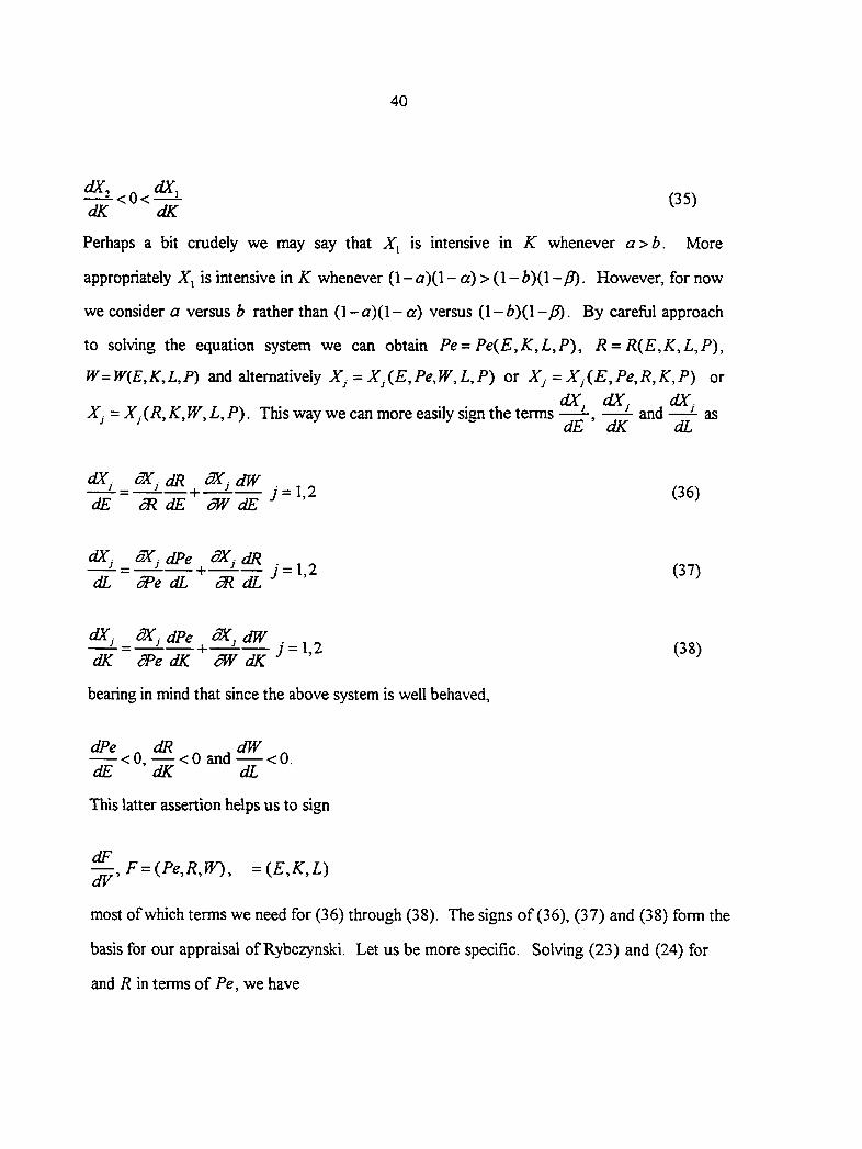
dX, dX, ^<0<^ (35) dK dK ^ ^
Perhaps a bit crudely we may say that is intensive in K whenever a>b. More
appropriately X^ is intensive in K whenever (1 - a)(l - a) > (1 - i)(l-p). However, for now
we consider a versus b rather than (l-a)(l- a) versus (1-Z>)(1-)^. By careful approach
to solving the equation system we can obtain Pe= Pe{E,K,L,P), R = R{E,K,L,P),
W=W{E,K,L,P) and alternatively Xj = Xj{E,Pe,W,L,P) or Xj = Xj{E,Pe,R,K,P) or
dX dX dX XJ = XJ{R,K,W,L,P). This way we can more easily sign the terms ——- and —- as
dX , SK. dR 3X. dw ^ = / = 1,2 dE cRdEaVdE
dX^ dPe dX. dR —L = —j = \ 2 dL dL gR dL
dE dK dL
(36)
(37)
dX. dPe dW — - = — 7 = 1 , 2 ( 3 8 ) d K ^ e d K c W d K ' ' ^ '
bearing in mind that since the above system is well behaved.
dPe dR ,dW • < 0, — < 0 and < 0.
dE ' dK dL
This latter assertion helps us to sign
^,F = (Pe,R,W), =iE,K,L) dV
most of which terms we need for (36) through (38). The signs of (36), (37) and (38) form the
basis for our appraisal of Rybczynski. Let us be more specific. Solving (23) and (24) for
and R in terms of Pe, we have
41
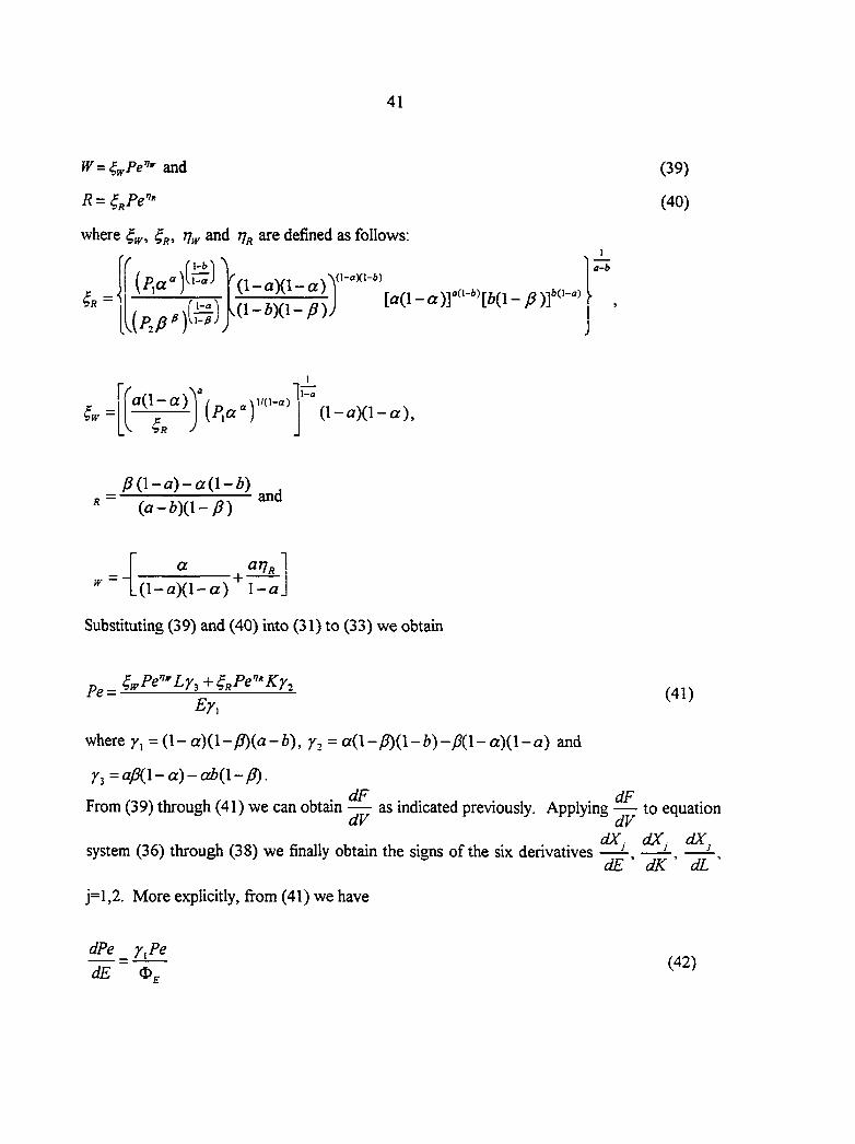
W = 4„Pe'" and
where and 7^ are defined as follows:
^(S)" ( P f i ' f
k^') fe)
O-aX' -g)
. (1- iXl-A)-
vd-oXl-i)
[a(l-a)]""-"[4(l-^)I fc(l-a)
1 a~b
(39)
(40)
gp-g) M{\-a)
1
\ -a
and
a ^Vr .(l-ar) ( l -a ) l -a .
Substituting (39) and (40) into (31) to (33) we obtain
^^_4^Pe'"Lr, + ,Pe'''Kr,
^Y\
where y^=(\- a)(l -yS)(a -b), y^- a(l -)S)(1 -h)- P{\ - a)(l - a) and
y^=ap{\-a)-ab{\-p).
dF dF From (39) through (41) we can obtain — as indicated previously. Applying — to equation
dX dX dX system (36) through (38) we finally obtain the signs of the six derivatives —
dE dK dL
j=l,2. More explicitly, fi^om (41) we have
dPe _ y Pe
'dE~~^ (42)
42
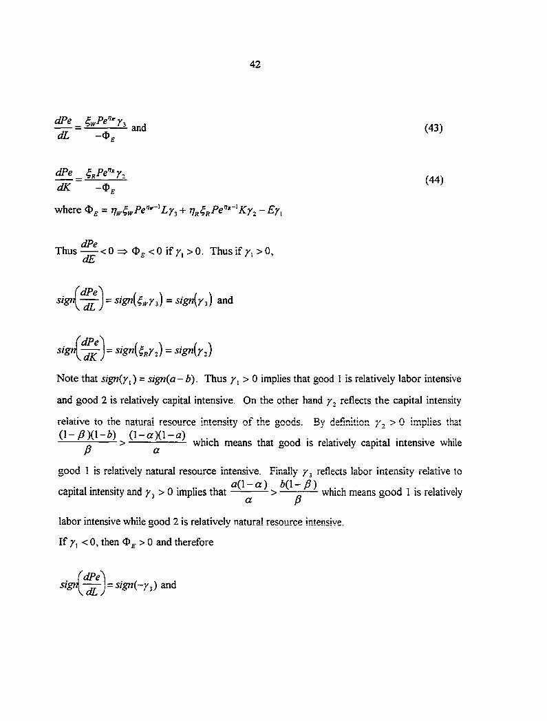
dPe J — and (43) dL -Og
dK -<i>,
-1 J- ~ « D^7*-I 1 where <D^ = rj^^^Pe^'-'Ly^ + Ky^ -Ey,
dPe Thus < 0 => O^. < 0 if 7, > 0. Thus if 7, > 0,
dE
sign ^dPe^ V d L ,
sign ^dPe
= sign(4^y^) = sign(y^) and
= = 'gn(r2) VdK
Note that sign{y^) = sign(a - b). Thus 7, > 0 implies that good 1 is relatively labor intensive
and good 2 is relatively capital intensive. On the other hand 7, reflects the capital intensity
relative to the natural resource intensity of the goods. By definition /, > 0 implies that ( l -y9) ( l -6) ( l -a ) ( l -a )
— > ^ which means that good is relatively capital intensive while
good 1 is relatively natural resource intensive. Finally y^ reflects labor intensity relative to a{\-a) b(\-B)
capital intensity and > 0 implies that —^— > ——— which means good 1 is relatively
labor intensive while good 2 is relatively natural resource intensive.
If y^ <0, then > 0 and therefore
fdPe^ J ^ and
43
=sign{-Y^) \aK y
Thus the above expressions suggest the following. If good 1 is relatively more labor
than capital intensive >0) and also relatively more labor than natural resource intensive
then an increase in the labor endowment increases the price of the natural resource input. An
increase in the capital endowment does the same if good 1 is relatively more resource than
capital intensive. Similarly, we can derive expressions for the impact of changes in factor
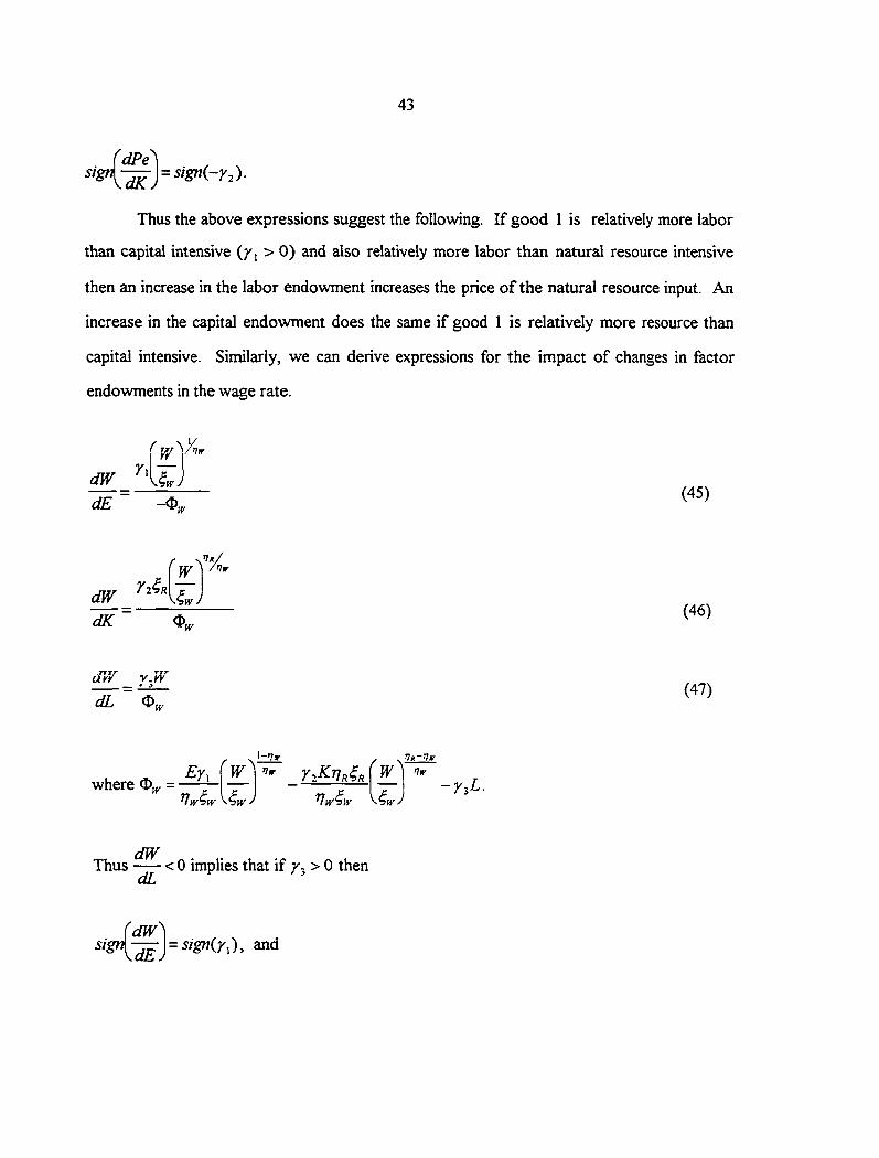
endowments in the wage rate.
dW
dE -d) (45)
dW _
dK ~ (46)
dV/ v.W * s (47) dL
where =
Thus < 0 implies that \i y~>0 then dL
(dW^ sigf\^j=sign{y,), and
44
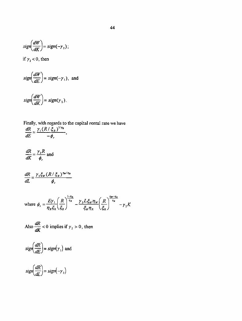
sign KdK
if ^3 < 0, then
= sign{-Y2)\
sign 'dW' [dE.
= sign(-r,), and
sign dK>
= sign{y,).
Finally, with regards to the capital rental rate we have dR_
dE -<!>,
dK
r,4^(.R'M"'" dL t
where <j>^ = Rl.
l-*?* r%i^^w'nw ( r ^ Hm
4R^r ^4RJ -72^
Also — < 0 implies if > 0, then dK
{^=sig,{-r,)
45
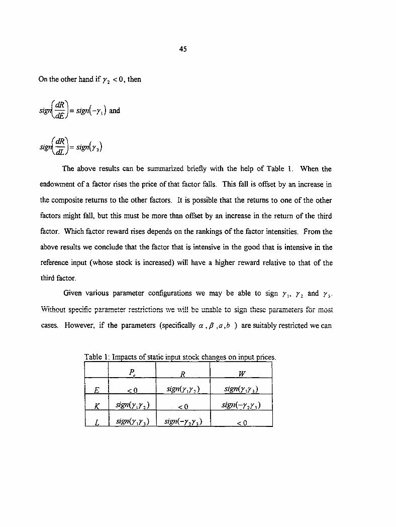
On the other hand if 7^2 < 0, then
= sign[-y^) and
sign = signir^) \dL.
The above results can be summarized briefly with the help of Table 1. When the
endowment of a factor rises the price of that factor falls. This fall is offset by an increase in
the composite returns to the other factors. It is possible that the returns to one of the other
factors might fall, but this must be more than offset by an increase in the return of the third
factor. Which factor reward rises depends on the rankings of the factor intensities. From the
above results we conclude that the factor that is intensive in the good that is intensive in the
reference input (whose stock is increased) will have a higher reward relative to that of the
third factor.
Given various parameter configurations we may be able to sign and /j.
Without specif.c parameter restrictions v/e will be unable to sign these parameters for most
cases. However, if the parameters (specifically a,,a,6 ) are suitably restricted we can
Table 1: Impacts of static input stock changes on input prices.
P. R W
E < 0 SIGNIYJ.)
K SIGNIJ.Y^) < 0 SIGRK-Y2R3)
L SIGNIYJ^) SIGFJI-Y^Y^) < 0
46
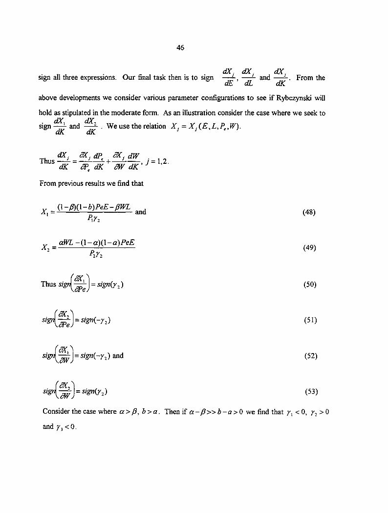
dX dX dX sign all three expressions. Our final task then is to sign ——- and —From the
dE dL dK
above developments we consider various parameter configurations to see if Rybczynski will
hold as stipulated in the moderate form. As an illustration consider the case where we seek to
sign and . We use the relation = Xj(E,L,P^,W). dK dK
dX dX dP 3>C dW . , , Thus —- = —7— , J = 1,2.
dK dK diV dK •'
From previous results we find that
^A^-m-h)PeE-pWL
^^2 (48)
aWL-(\-a){\-d)PeE
P2n (49)
Thus J = signir^) (50)
,
( 5 1 )
sigt: dfVj
= sign(-y^) and (52)
SlgtJ = sign(y^) (53)
Consider the case where cc>/3, b> a. Then if a-j3»b-a>0 we find that T', < 0, 7', > 0
and Y2<0.
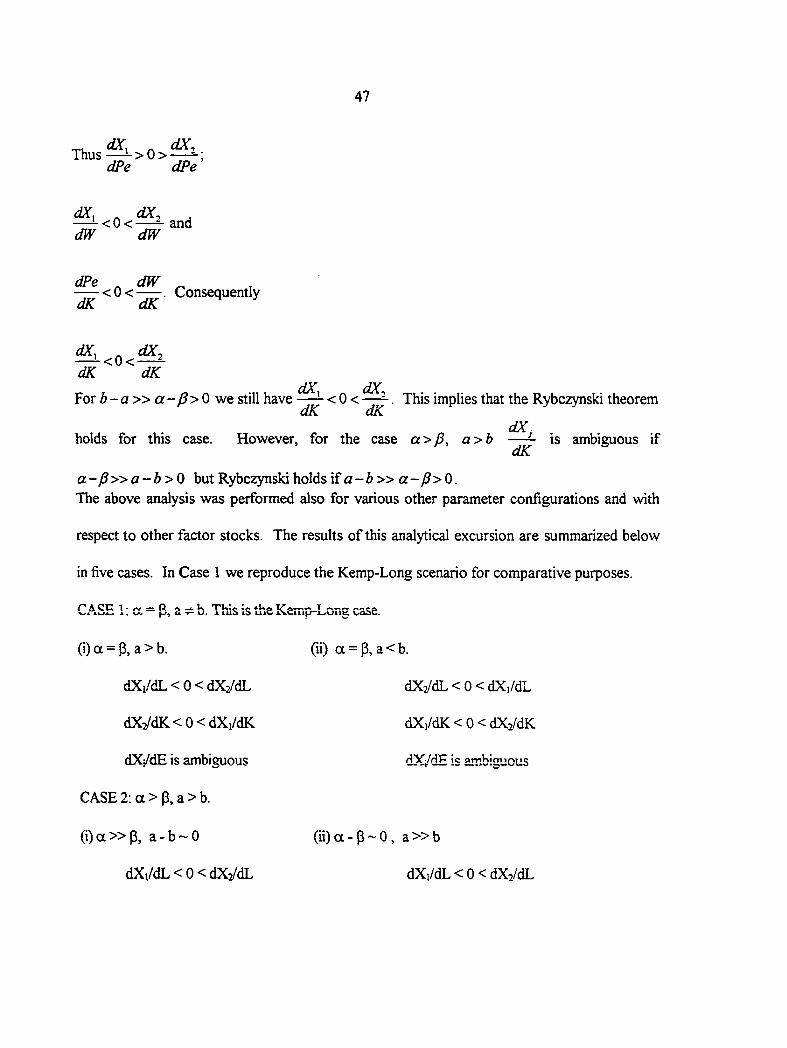
47
dX, ^ dX. Thus —^ > 0 > —
dPe dPe'
dX, dX. ^<0<^ and dW dW
dPe dW <0< . Consequent ly
dK dK
dX, ^ dX^ —^<0<-—^ dK dK
dX dX For b-a» a-p>0 we still have < 0 < . This implies that the Rybczynski theorem
dX holds for this case. However, for the case a>p, a>b —- is ambiguous if
dK
a-p » a-b>0 but Rybczynski holds if a - 6 » a - > 0. The above analysis was performed also for various other parameter configurations and with
respect to other factor stocks. The results of this analytical excursion are summarized below
in five cases. In Case 1 we reproduce the Kemp-Long scenario for comparative purposes.
CASE 1: a = P, a b. This is the Kemp-Long case.
(i)a = p, a>b.
dXi/dL<0<dX2/dL
dX2/dK<0<dXi/dK
dX^dE is ambiguous
CASE 2; a > (3, a > b.
( i ) a » P , a - b ~ 0
dXi/dL<0<dX2/dL
(ii) a = p, a < b.
dXz/dL < 0 < dXi/dL
dX,/dK<0<dX2/dK
dX/dH is Hrnbis^wCus
(ii) a - P ~ 0, a » b
dXi/dL<0<dX2/dL
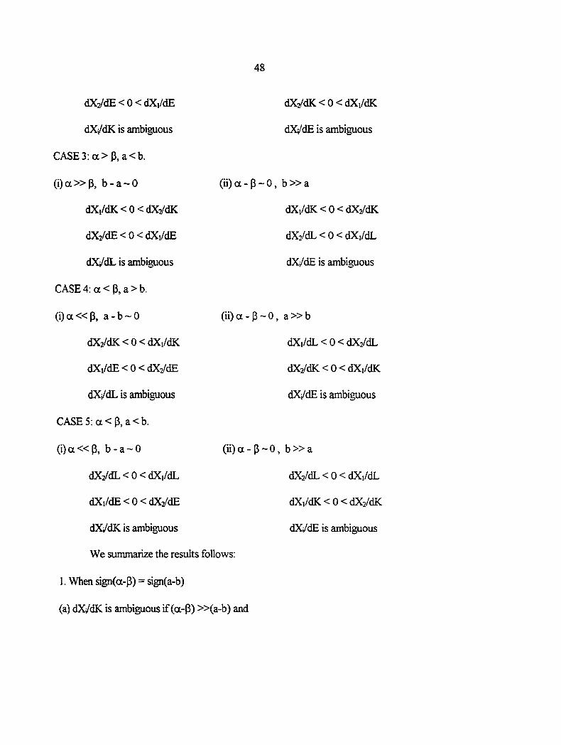
48
dX 2/ciE< 0<dXi/dE
dX/dK is ambiguous
CASE3: a> P, a<b.
( i )a»P, b-a~0
dX, /dK<0 <d X2/dK
dX2/dE<0<dXi/dE
dXi/dL is ambiguous
CASE 4: a < P, a > b.
( i ) a « P , a - b ~ 0
dX2/dK<0 <d X i/dK
dXi/dE<0<dX2/dE
dXi/dL is ambiguous
CASE 5; a < P, a < b.
( i ) a « P , b - a ~ 0
dX2/dL<0 <d X i/dL
dXi/dE<0<dX2/dE
dXi/dK is ambiguous
dX2/dK<0 <dXi/dK
dXi/dE is ambiguous
( i i )a -P~0, b»a
d Xi/dK<0 < d X2/dK
dX2/dL<0<dX,/dL
dX/dE is ambiguous
( i i )a -P~0, a»b
dXi/dL<0 <dX2/dL
dX2/dK<0<dX,/dK
dX/dE is ambiguous
(ii) a - P ~ 0, b » a
dX2/dL<0 < d X ,/dL
dXi/dK<0<dX2/dK
dXi/dE is ambiguous
We summarize the results follows:
1. When sign(a-P) = sign(a-b)
(a) dX/dK is ambiguous if (a-P) »(a-b) and
49
(b) dXi/dE is ambiguous if (a-|5)« (a-b).
2. When sign(a-P) = sign(b-a)
(a) dXi/dL is ambiguous if (a-P) »(b-a) and
(b) dXi/dE is ambiguous if (a-P)« (b-a).
Thus we find that there are regions where Rybczynski holds and regions where the
result is ambiguous. Ambiguity here is not proof that Rybczynski does not hold. The latter
can only be ascertained when exact parameter values and factor levels are given. To obtain a
more comprehensive characterization of the moderate version of Rybczynski we performed
computer simulations over the parameter space. Fixing and 6 = we varied a, a, and
the factor stock levels to see where Rybczynski-like results hold and where anti-Rybczynski
results pertain. The computer simulations were programmed in Maple and the input is
presented here as Appendix 1. The results of the simulations enable us not only to show that
the Rybczynski theorem does not hold in some cases but also to obtain the more useful
information of knowing where in the parameter space it holds and where it does not.
From the above results we arrive at the following propositions
Proposition 1:
(a) When natural resource intensities differ across the two goods, the static version of
Rybczynski does not necessarily hold.
(b) Given our technological assumptions, the static version of Rybczynski may not hold for
(i) a capital stock increase if the good that is intensive in capital is also intensive in the natural
resource input.
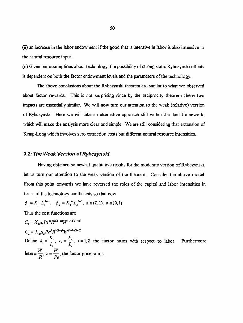
50
(ii) an increase in the labor endowment if the good that is intensive in labor is also intensive in
the natural resource input.
(c) Given our assumptions about technology, the possibility of strong static Rybczynski effects
is dependent on both the factor endowment levels and the parameters of the technology.
The above conclusions about the Rybczynski theorem are similar to what we observed
about factor rewards. This is not surprising since by the reciprocity theorem these two
impacts are essentially similar. We will now turn our attention to the weak (relative) version
of Rybczynski. Here we will take an alternative approach still within the dual framework,
which will make the analysis more clear and simple. We are still considering that extension of
Kemp-Long which involves zero extraction costs but different natural resource intensities.
3.2: The Weak Version of Rybczynski
Having obtained somewhat qualitative results for the moderate version of Rybczynski,
let us turn our attention to the weak version of the theorem. Consider the above model.
From this point onwards we have reversed the roles of the capital and labor intensities in
terms of the technology coefficients so that now
a e(0,l) , b g(0,1).
Thus the cost functions are
C, =
C, =
K E Define i-, / = 1,2 the factor ratios with respect to labor. Furthemiore
L . 4 W W
letfij s — A = — the factor price ratios. R P e ^
51
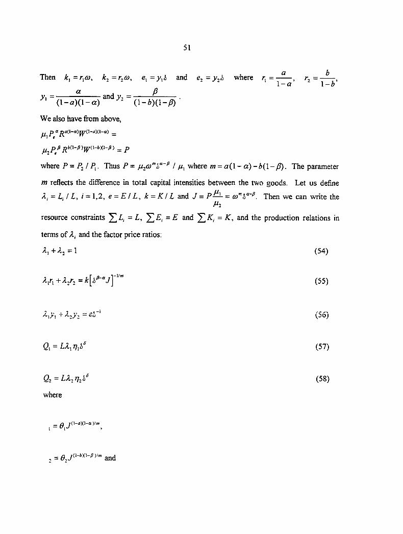
Then k^=r^co, k^=r^(o, e, =3/,^ and ^2 =>'2'^ where r, = , /*, = , \ - a \ - b
« J P V, = and V, = .
We also have from above,
where P - P ^ l P ^ . Thus P = / /i, where /n = <3(1 - a)-6(1 -/?). The parameter
m reflects the difference in total capital intensities between the two goods. Let us define
= L j I L , i - 1,2, e - E I L , k = K I L and J = P— = Then we can write the )"2
resource constraints ^ A — ~ ^ = K.-, and the production relations in
terms of and the factor price ratios:
A , + ^ 2 = 1 ( 5 4 )
A,r, + IjA = kU^^jY" (55)
+ 2/2 ~
0; = LAj 77ji^ (57)
0^=LX2T]^h' (58)
where
. = 9,f
. = and
52
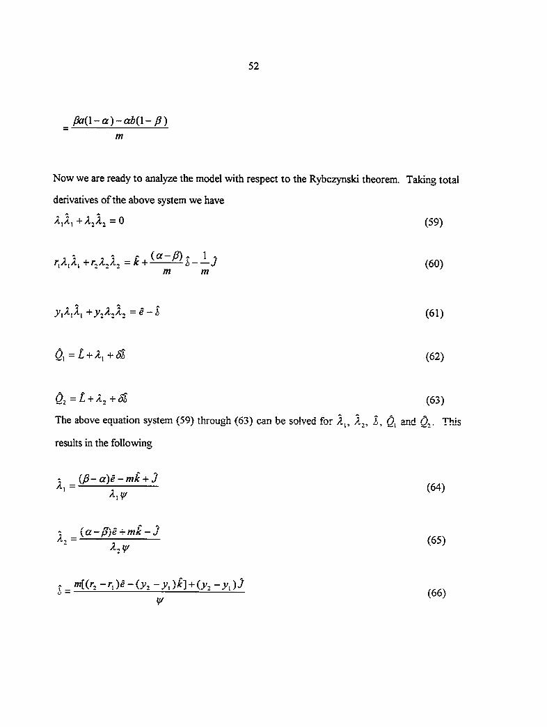
Pa{ \ -a ) -c ib( \ - P ) m
Now we are ready to analyze the model with respect to the Rybczynski theorem. Taking total
derivatives of the above system we have
+^2^2=0 (59)
r (a-/5) 7 1 =k + - J (60)
m m
+3;jA,1, =e-i (61)
0, = £ + A, + ^ (62)
0^=l, + A^+Si (63)
The above equation system (59) through (63) can be solved for A,, A,, I, 0, and This
results in the following
1 _ {p-a)e-mk + 3 ^1 1 (64)
X,y /
^ J-J ^ ' '^h ' 1 _KCi -p) i :^ /nK- j ^2 ; (65)
T _ " ' [ ( r . -Oe- iy^-y , )k ] + iy^-y^)J o —— (66)
y/
53
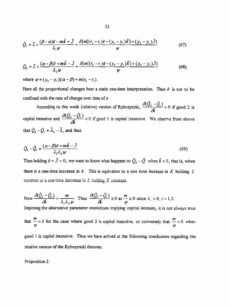
' A, ^ \f/
^ ^ {a -P)e+mk-J ^ 5 {m[{r^- r , )e - iy^-y , )k} + {y^-y^)3)
^ X^if/ If/
(67)
(68)
where ?/= (>'2-;',)(a-y^ + /w(rj-r,).
Here all the proportional changes bear a static one-time interpretation. Thus e is not to be
confused with the rate of change over time of e.
According to the weak (relative) version of Rybczynski, —> 0 if good 2 is
) capital intensive and —< 0 if good 1 is capita! intensive. We observe from above
that ^2 - = ^2 - A, and thus
(69) XjAj y/
Thus holding ^ = J = 0, we want to know what happens O1-O when ^ > 0, that is, when
there is a one-time increase in k . This is equivalent to a one time increase in K holding L
constant or a one time decrease in L holding K constant.
.^ ^0, -(5,) m d{0 . -0 , ) . , Now — > = -7-^; . Thus — . ~ > 0 as — >0 smce A, > 0, / = 1,2.
3c A^A^y/ S i y / Imposing the alternative parameter restrictions implying capital intensity, it is not always true
that — > 0 for the case where good 2 is capital intensive, or converselv that — < 0 when ¥ - ' ' y/
good 1 is capital intensive. Thus we have arrived at the following conclusions regarding the
relative version of the Rybczynski theorem.
Proposition 2;
54
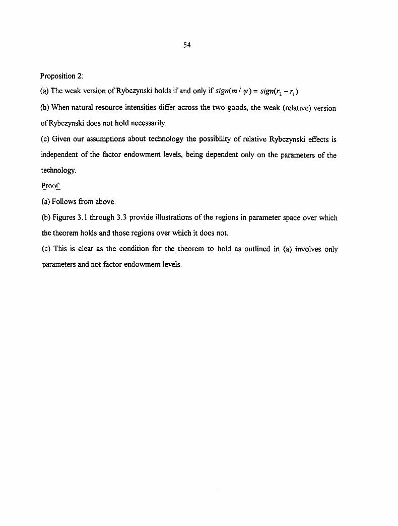
Proposition 2:
(a) The weak version of Rybczynski holds if and only if sign{m I ij/) = sign(r^ - r,)
(b) When natural resource intensities differ across the two goods, the weak (relative) version
of Rybczynski does not hold necessarily.
(c) Given our assumptions about technology the possibility of relative Rybczynski effects is
independent of the factor endowment levels, being dependent only on the parameters of the
technology.
Proof:
(a) Follows from above.
(b) Figures 3.1 through 3.3 provide illustrations of the regions in parameter space over which
the theorem holds and those regions over which it does not.
(c) This is clear as the condition for the theorem to hold as outlined in (a) involves only
parameters and not factor endowment levels.
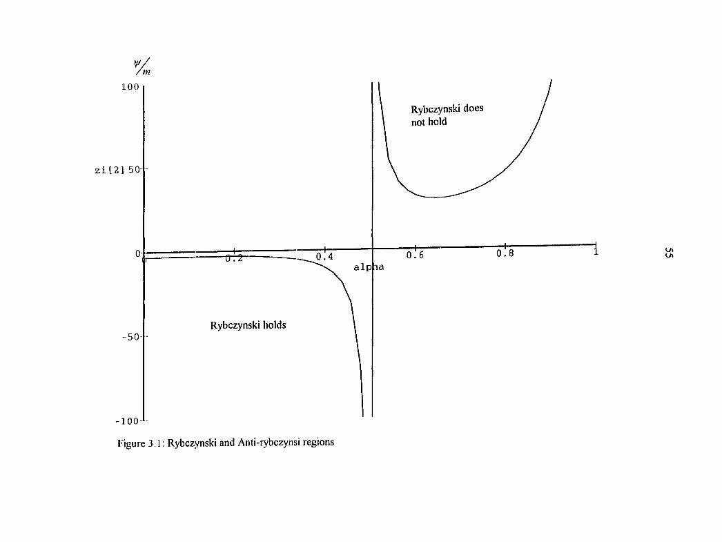
V /m 100
z i [ 2 ] 5 0 -
-Ot2- 0 . 4 a l p lia
• 5 0 -Rybczynski holds
- 1 0 0 -
Figure 3.1: Rybczynski and Anti-rybczynsi regions
Rybczynski does not hold
0 . 6 0 . 8 v/i
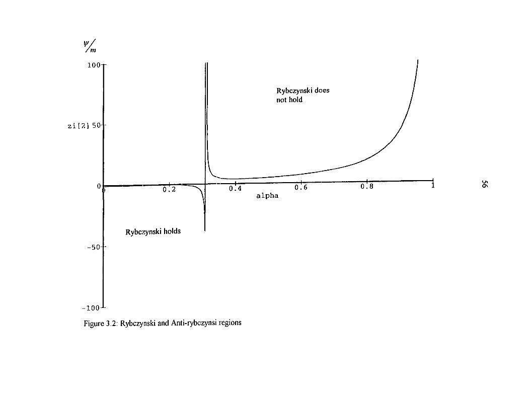
/m
1 0 0 -
z i [ 2 1 5 0 -
0 . 2 0 . 4
Rybczynski holds
- 5 0 - -
-100-^
Figure: 3.2: Rybczynski and Anti-rybczynsi regions
Rybczynski does not hold
0 . 6 Ipha
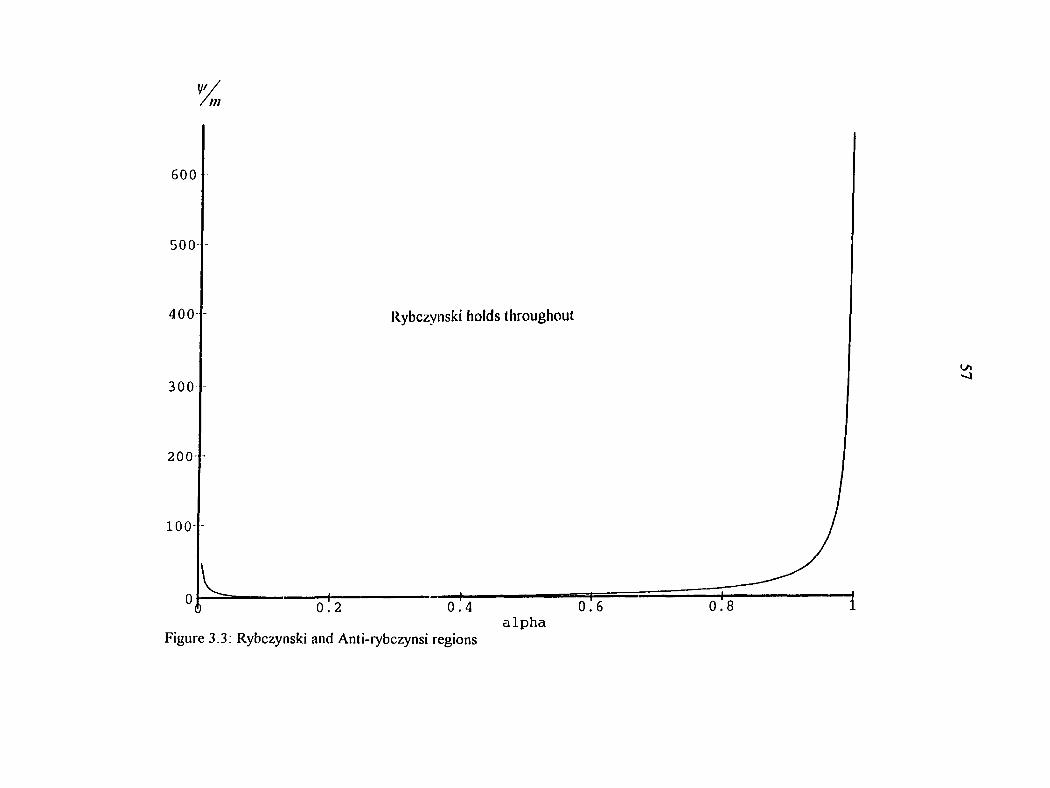
600
500
400- Rybczynski holds throughout
300
2 0 0 -
1 0 0 -
alpha Figure 3.3; Rybczynski and Anti-rybczynsi regions
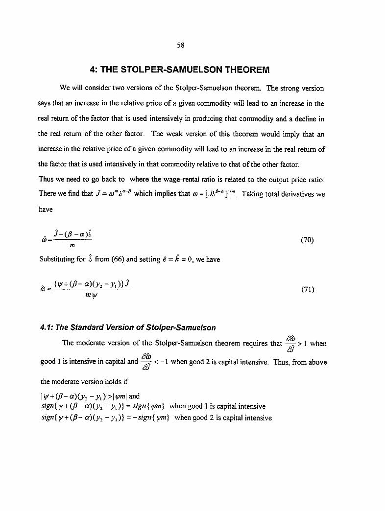
58
4: THE STOLPER-SAMUELSON THEOREM
We will consider two versions of the Stolper-Samuelson theorem. The strong version
says that an increase in the relative price of a given commodity will lead to an increase in the
real return of the factor that is used intensively in producing that commodity and a decline in
the real return of the other factor. The weak version of this theorem would imply that an
increase in the relative price of a given commodity will lead to an increase in the real return of
the factor that is used intensively in that commodity relative to that of the other factor.
Thus we need to go back to where the wage-rental ratio is related to the output price ratio.
There we find that J = which implies that co = [Jh^" Taking total derivatives we
have
. J+{P-a)h a = — (70)
m
Substituting for i from (66) and setting e = ^ = 0, we have
^_ W+{p-a) {y2 -y , ) }3 mil/
4.1: The Standard Version of Stolper-Samuelson d(b
The moderate version of the Stolper-Samuelson theorem requires that —> 1 when
good 1 is intensive in capital and —r < -1 when good 2 is capital intensive. Thus, from above aJ
the moderate version holds if
\V+ip-a){y2 -.yi)l>IV^i and sigri{iif+{p- a)(y2 ->'i) } = s i g n { y m ) when good 1 is capital intensive
sign{ \}/+ (fi- a){y^^ - >'i)} = -sign{ ym} when good 2 is capital intensive
59
Recall that Y={y2-y\){cc-p)-^ - fx) which implies that
i f f + i f i - a ) i y 2 - > ' , ) = m i r ^ - / • , ) •
Therefore for the theorem to hold we must have Ir^ -r,l>lv'| and sign{r^ -r^) = sign{\f/)
when good 1 is capital intensive and sign(r2 -r^) = -sign{ y/) when good 2 is capital
intensive. Recalling the definitions of = 1,2, we see that neither of these necessarily
holds. We summarize the above in the following proposition.
Proposition 3:
a: The moderate version of Stolper-Samuelson holds if and only if |r, - r, 1>| and
(i) signir^ ~ ''i) = ¥) when good 1 is capital intensive or
(ii) signir^ -r^) = -sign{ y/) when good 2 is capital intensive.
b: When the two goods are different in their natural resource intensities the standard
(moderate) version of the Stolper-Samuelson theorem does not hold necessarily.
4.2: The Weak Version of Stolper-Samuelson
The weak version requires that > 0 <=> s i g n ( r ^ ~ f ] ) = s ' g f K y ^ ) when good 1 is
^0) capital intensive and —< 0 <=> sign{r^ ~f\) = ¥) when good 2 is capital intensive.
<2/
This in turn implies that y / < Q \ n both cases. Thus we arrive at the following.
Proposition 4a;
Weak Stolper-Samuelson holds if and only if ^ < 0.
Simulation results show that for all parameter values ^^<0, as exemplified in Figure 4.1
which displays a plot of y/ against a for given values of the other parameters. Thus we can
say the following.
60
Proposition 4b:
The weak version of the Stolper-Samuelson theorem holds even when natural resource
intensities differ across the two goods.
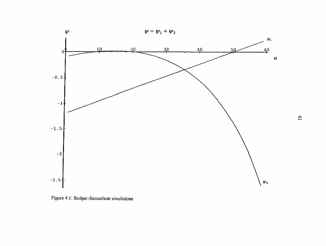
y/ y /=y^x + Wi
- 1 . 5 - -
-2 -
- 2 . 5 -
Figure4.1: Slolper-Samuelson simulations
o\
^2
62
5: THE GENERALIZED H-0 MODEL WITH EXTRACTION COSTS
In the previous section we extended the generalized H-0 model by allowing for
different natural resource intensities across the two goods. In this section we shall revert back
to the case where the natural resource intensities are the same but extend the model by
allowing for positive marginal costs of extracting the natural resource input. We shall assume
that the natural resource input is extracted with the use of positive amounts of labor and
capital. Specifically, the description for our technology becomes
X . = Z , , a n d
A', = as in Kemp-Long. But now we also have
E = g { K ^ , L ^ ) = Maintaining our dual approach, the cost functions are
respectively:
C, = (72)
C = and (73)
Cj = (74)
o. b y Mrnoro Ir — y—- >• — . y — - ^ I /v^ — t — 1^1 ' 2~ i L ' 3~1 '
/ = = and y-, and co and h are as defined previously. ( l-a)(l-a) - ( l-6)(l-a)
J = — P = co" where now /n = (1 - a)(a - b) and P= P^ / P, dis previously defined. M2
Define (75)
the net shadow price of the natural resource input. Thus
^ - r , , y + M-,0} n = \. (76)
63
Expressing as before the factor constraints and technology relations in terms of the
factor prices and parameters, we obtain the following system of equations:
A,+A,+A3 = 1 (77)
M + 2^2 + ^3^3 = (78)
Vl +>^2^2 (79)
!• + ,., A/-"- = (80)
• 'e
= e where 73 = Tj'' (81)
Q^^LX,T],h' ' (82)
0^=LX.Ti^h'' (83)
Taking total derivatives as before we get
+ A, + AjAj = 0 (84)
J r,2,A, +r^2,A, = k (85)
m
>',2, A, = e-i (86)
d - P , - - J = e (87) m
^, = Z + Ij + ai (88)
Oj — L, + •!" (89)
We can solve for 1,, /" = 1,2,3, 1,0^,0^^ and as
^ fn tn
64
) + (r, -r^)?.^{e + J)
^2 = —^-^-7 —— (91) ^l iT i - rx )
-rd + ^yx ->'2)(^--)-'^3(>'l ->'2 +''3)(e + --/) OT m
' • i - rx (92)
(^--^ + e)(r, -r ,) + (j ' ,->'2)(^--)-A3(;; , -J 'z+r3)(e + -J) w m L (93)
^2 -^,
J A, (£ + Qis)(r, - r,) + (^ —XaCy, -><2) A, -1] - A, (^ + -^ J)[a;i, {y, ->', + ) + (r^ - rj)]
^ ^ ^ ( 9 4 ) A,(r, -r,)
(Z + a?)(rj - r,) + (^ - -)[a(y, - )/l, +1] - A3 (^ + - J)[aA, (y, - :V2 + /"j) - (n - /"j)] a = ^ 77 ^^ (95)
/l,(r, -r,)
Given the foregoing we are ready to arrive at some conclusions regarding the
RybczjTiski and Stolper-Samuelson theorems.
5.1: The Standard Version ofRybczynski
From above.
a(V. - v. \Z . - \ ^' and (96)
^ A.J (r, - r,)
^2 ^ ->'2)^2 +1
-^2 ('2 ~ ''i) (97)
We note that
65
a C r ^ - r , ) a { b - a ) _ y2-yx= -yzrx = , , ' = , , , r- Thus
(1-a) (l-a)(l-6)(l-a)
SO, ^g^^(r,-r,)/0-g)-l
d Mf2-n)
Similarly,
a- 1
1 - a (98)
^2 1 Q;" ^ (99)
i ,(r ,-r ,) (l-a)
Suppose good 2 is capital intensive. Then r, > r, and we have —=^ < 0 as needed for
Rybczynski. However, —appears ambiguous from the above expression. In the same vein,
for good 1 being capital intensive, r, < r, implying that < 0 as required, but now— ^ dc
appears ambiguous.
However, this ambiguity in both cases is only apparent. Consider a one time increase
in k. Given that the factor constraints hold exactly suppose the increase in k is not applied to
X, or production. Then it must be used for E. In that case, however, the resulting
increase in e means that e to be used in X, or X, since the natural resource input is assumed
to be nontraded. This contradicts our earlier assertion that the increase in k is not applied to
either or X^. Granted now that an increase in k is used to produce at least one of X, or
X,, —< 0 established implies that > 0 when good 2 is capital intensive. Similarly
dC) sC) for good 1 being capital intensive, < 0 => -=^ > 0. Thus we conclude that the moderate
version of the Rybczynski theorem holds.

66
Proposition 5:
When the natural resource intensities are the same across the two goods, the Rybczynski
theorem holds in the absence of trade in the natural resource input even when there are
positive marginal costs of extraction.
This proposition implies that the weak version of Rybczynski holds as well in this case. This
is easier to establish since we have
( i f - - ) ( l - ; i3 ) + l3 (e + J ) (AJ- '"" - r , ) ttt 000)
1-^ ^ 0 as good 2 and hence — = —— „ , , is capital mtensive.
a: -/- ,)< 0 as good 1 ^
5.2; r/ie Stolper-Samuelson Theorem
Establishing the Stolper-Samuelson theorem is more obvious since from above, .J
J — of which implies that d) = —. Now signt^m) = sign{a - b). Furthermore j.'T'ie (0,1) and m
hence we conclude the following;
Proposition 6;
When natural resource intensities are the same across the two goods, the strong version of
Stolper-Samuelson holds regardless of extraction costs of the Cobb-Douglas form.
Proposition 6 implies that the weaker versions of the Stolper-Samuelson theory hold as well.
67
6: CONCLUSION
In this paper we have investigated the implications for standard static trade theorems
of allowing for different natural resource intensities in the framework of the Kemp-Long
generalized H-0 model. We found that the Rybczynski and Stolper-Samuelson theorems no
longer hold in general. Various versions of the theorems were considered - strong and weak
versions - and the conditions under which these hold were analyzed.
The above conclusions held in the absence of extraction costs. It was found that when
positive extraction costs were allowed for, but reverting back to the equal natural resource
intensities assumption of Kemp-Long, the standard static trade theorems were upheld. Thus
the issue of more importance here was that of factor intensity rather than extraction
technology. A necessary caveat though, is that our extraction technology was restricted to be
of Cobb-Douglas constant returns form so that the results might not be generalizable to other
forms of extraction technology.
68
7: REFERENCES KEMP, Murray C. and Ngo van Long; The Role of Natural Resources in Trade Models, in Handbook of International Economics, R. W. Jones and P. B. Kenen (eds.), North-Holland, 1984.
KEMP, Murray C. and Ngo van Long; "Rybczynski's Theorem in a Context of Exhaustible Resources; The Case of Time-Contingent Prices', International Economic Review Vol.23, No.3 (October, 1982): 699-710.
KEMP, Murray C. and Ngo van Long; International trade with an exhaustible resource: A theorem ofRybczynski type. International Economic Review, Vol.20, No.3 (October, 1979), 671-677.
KEMP, Murray C. and Ngo van Long; Exhaustible resources and the Stolper-Samuelson-Rybczynsld theorems. Essay 14 in Exhaustible Resources, Optimality, and Trade, Kemp and Long (eds) (North-Holland Publishing Company, Amsterdam, 1980)
SEGERSON, Kathleen, "Natural Resource Concepts in Trade Analysis", in Agricultural Trade and Natural Resources: Discovering the Critical Linkages, John D. Sutton (ed.), Lynne Rienner Publishers, 1988.
69
PAPER 2:
DYNAMIC ISSUES IN
THREE EXTENSIONS OF THE GENERALIZED H-0 MODEL
70
1; INTRODUCTION
1.1: Background
Various alternative models have been used to incorporate natural resources into trade
models. Kemp and Lxjng (1984) surveyed the existing literature and provided a summary of these
models. On the opposite extreme from the standard H-0 firework is the class of Anti H-0
models in which the two Ricardian (primary) inputs of the traditional H-0 model are replaced by
two raw materials obtained from a natural resource stock. Thus two final goods are produced
nonjointly by two Hotelling factors using a constant returns to scale technology. Hybrid models
are those in which one of the two inputs is Ricardian and the other is Hotelling. Generalized
models have at least one of each type of input. In Generalized H-O models there are two Ricardian
factors and at least one Hotelling factor, possibly many. Generalized anti H-0 models have two
Hotelling factors and at least one Ricardian factor. While all these models could to various
extents, be employed for useful analysis, most of the works in the literature have used the anti H-0,
hybrid, and generalized H-0 models (hereafter GHOM)-
The anti H-0 model allows one to investigate static and dynamic issues in a two sector
trade model when the only inputs are two different raw materials obtained from a natural resource
stock. Except in singular cases the two goods will differ in their respective intensities in the two
inputs. Thus the economic implications appear much the same as in the traditional H-0 perspective
except that the usual static analysis is now appended by dynamic considerations.
The hybrid model provides a dimension of analysis not included in the anti H-0 model.
With the former, the opportunity is presented for us to analyze trade and production issues in a
situation where one of the inputs is obtained from a stock of endowment that is fixed over time
while the other is obtained from a stock that varies (usually falls) over time.
71
The GHOM is a further improvement over the anti H-0 and hybrid models for most
purposes. By simply appending a hotelling factor to the traditional H-O model, the GHOM allows
us to analyze the static issues of the traditional H-0 model more fiilly than does the hybrid model:
we can consider issues pertaining to different factor intensities when two factors are Ricardian.
Since the third factor is hotelling we are able to consider the dynamic issues that the hybrid models
also pemiit. In short, the GHOM more completely embodies the technolo^cal possibilities that
might be of interest to us. As such we have chosen, in this paper as well as in others, to provide
useful extensions to the GHOM of Kemp and Long (1984) as our contribution to the existing body
of literature.
Naturally, dealing with more than two factors of production means that the usual
propositions which are formulated in terms of relative factor intensities and relative factor
abundance are expected to be much more complicated. Thus work on the GHOM has proceeded
by imposing a suitably restrictive structure on the production technologies. Proceeding in this
fashion Kemp and Long (1980, 1984) established dynamic counterparts of all the major trade
theorems (Heckscher-Ohlin, Stolper-Samuelson, Rybczynski and Factor Price Equalization). In
particular, they assumed a production function of the form
X. = X^iE.,L^,K^) = E;0^iL^,K^y-' ' j = 1,2. (1)
so that the natural resource intensities are restricted to be the same across the two goods.
As our first extension of the GHOM we relax this assumption by allowing for different
natural resource intensities. Our task then will be to characterize some useflil propositions
concerning production patterns and trade. Another promment assumption of the work of Kemp
and Long with the GHOM is that of costlessness of extraction. In the second extension we will
allow for positive marginal costs of extraction but revert to the assumption of equal natural
resource intensities. The final extension will be a combination of the first two; we will consider the
72
Kemp-Long GHOM with different natural resource intensities and positive mar^al extraction
costs.
At this stage it wll be helpful to spell out the basic assumptions that we use throughout the
paper.
1.2: Basic Assumptions
1.2.1: Production Structure
The most obvious assumption underlying this paper is that of functional structure. We will
follow Kemp-Long (1984) in using the Cobb-Douglas structure freely in all sections of this paper.
Each good, Xj, is produced with a natural resource input, Ej and an intermediate good Oj. Oj is
in turn produced using labor Lj and capital Kj. In the Kemp-Long study no specific structure was
specified for Oj (Lj ,Kj). However, for expositional ease we will use the Cobb-Douglas structure
again for Qj(Lj ,Kj). This resuhs in just a slight loss of generality but it pays off with significant
ease of analysis. Our final use of the Cobb-Douglas stmcture is in the specification of the
extraction technology' in sections I! and HI where we assume positive marginal extraction costs. A
modest defense of the use of the Cobb-Douglas production functions in such analysis has been
provided in Kemp and Long (1980). Each production flinction exhibits strict quasi-concavity and
constant returns to scale. There is no capital investment and the natural resource stock is assumed
to be exhaustible.
1.2.2: Price and Market Structure
Competitive market conditions prevail, as also assumed in the standard H-0 model.
Furthermore, we shall assume that final good prices are exogenously given and constant. The case
73
of time contingent prices has been investigated by Kemp and Long (1982) in the framework of the
hybrid model.
1.2.3: Borrowing and Lending Possibilities
Throughout this paper we shall assume that perfect borrowing and lending conditions
prevail in international capital markets. This implies that the maximization of the discounted stream
of output is necessary for the maximization of discounted utility (Segerson, 1988).
In addition to the above we maintain the H-0 assumption of identical preferences within a country
and across countries.
Having outlined the basic assumptions a word about our method of approach is usefLil.
1.3: Methodology
We have chosen, throughout this paper to use a dual approach in our analysis. This
approach appears much easier and more insightful. Furthermore, the analysis is flirther simplified
by splitting the entire optimization problem into three phases;
Phase 1 A; Static optimization over labor and capital inputs to produce the imermediate goods,
and O2.
Phase IB; Static optimization over the natural resource input, E to produce the two final goods,
Jr, and Z,.
Phase 2; Dynamic optimization to choose the path of natural resource extraction, E(t), that
maxin^es the discounted present value of income.
In this paper we shall dwell on dynamic issues. Static issues have been addressed in another paper.
74
2: THE GHOM WITH DIFFERENT RESOURCE INTENSITIES AND ZERO EXTRACTION COSTS
As mentioned earlier in the section on methodology, we start with intermediate good
production and then proceed to consider final good production.
2.1: Intermediate Good Production
It will be useful to see the production of the two final goods as composed of two phases of
production. First, the production of the intermediate goods using the primary factors and secondly
the utili2ation of the intermediate goods in final good production. Let the production function for
the intermediate goods be written as
o, = L;^K; -^^i= \x (2)
Let W and R be the respective wage and capital rental rates, and let and 5, be the surrogate
prices of 0, and . The cost fiinction dual to this production structure has a familiar form;
TC^ = j=l,2 (3)
where 6j = (1 - Qjj .
By the H-0 assumption of perfect competition
ffrc S, < j=l,2 (4)
with equality when Oj > 0 j=l,2. Thus as long as both intermediate goods are produced (4)
represents a system of two simultaneous equations which can be solved to yield the factor price
levels as functions of the intermediate good prices;
75
W = and (5)
R =
I
r (5 , /e ,Y ' r"*"
L f e ' « , r j •
Hence the wage rental ratio, co is given as
(6)
W CO =
0,5,
5, Define p= —, the ratio of intermediate good prices. Then
CO = e,
"a
1
«2-«I (7)
Thus at the level of intermediate good production the relationship between primary factor
prices and the intermediate good price ratio obeys the Stolper-Samuelson theorem. Applying
Shepherd's lemma to (3) we obtain the optimal input allocations
' W (8)
I (9)
The returns to the labor and capital inputs are constant shares of the value of intermediate good
and these shares sum up to 1 as one would expect from the assumption of constant returns to scale.
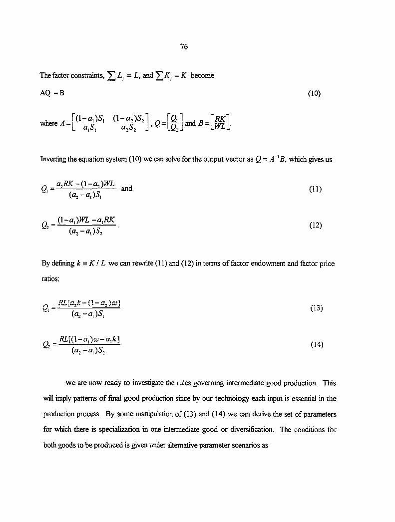
76
The factor constraints, ^ L j = L , and ^ K j = K become
AQ =B (10)
where 0 «2)'^2 *2*^2
and B = [rk ' IWL,
Inverting the equation system (10) we can solve for the output vector as O = A B, which gives us
0,=2a«£dlz£l)51 and (a,-a,)S,
(11)
_ ( \ - a , ) W L - a , R K
(a,-a,)5. (12)
By defining k = KI L we can rewrite (11) and (12) in terms of factor endowment and factor price
ratios;
Q^ = RL[{\ - a^)o}- a^k] (14)
We are now ready to investigate the rules governing intermediate good production. This
will imply patterns of final good production since by our technology each input is essential in the
production process. By some manipulation of (13) and (14) we can derive the set of parameters
for which there is specialization in one intermediate good or diversification. The conditions for
both goods to be produced is g^ven under alternative parameter scenarios as
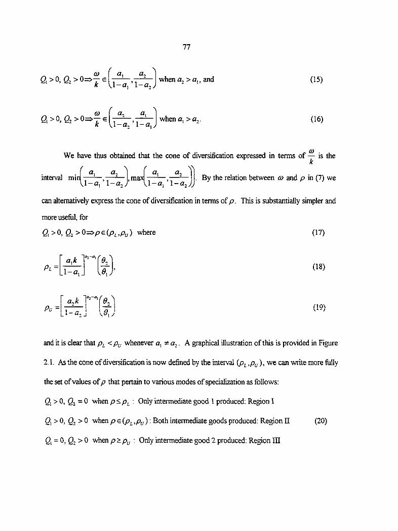
77
0) Q, > 0, 02 > 0=>— e
a,
.1-a, '1-a, when <ar, > a,, and (15)
0) Q >0, 02 >0=>—e
a,
,1-a, '1-a when a, >a,. (16)
We have thus obtained that the cone of diversification expressed in terms of y is the
f \ f interval min
a,
vl-a, '1-a, .max
a, a, , — — . B y t h e r e l a t i o n b e t w e e n O) and p in (7) we
J-a, l -a^JJ
can alternatively express the cone of diversification in terms of p. This is substantially simpler and
more useful, for
0, >0, Oj >0=>pG(p^,Py) where (17)
Pl = a^k
-l-«i- ^^1J a,k T=-"'
1 1 L ^
1 J
(18)
/ ' io\
and it is clear that p^ < whenever a, a,. A graphical illustration of this is provided in Figure
2.1. As the cone of (^versification is now defined by the interval (p^ ), we can write more fiilly
the set of values of p that pertain to various modes of specialization as follows:
0, > 0, O2 = 0 when p<Pi : Only intermediate good 1 produced: Re^on I
Qi > 0, Oj > 0 when p e ): Both intermediate goods produced: Region n (20)
Qi = 0, Q2 > 0 when p> p^ : Only intermediate good 2 produced: Re^on HI
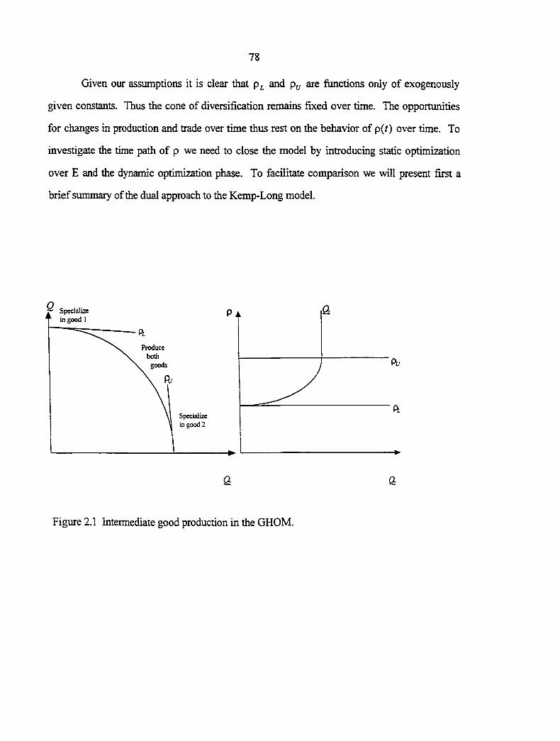
78
Given our assumptions it is clear that and Py are functions only of exogenously
given constants. Thus the cone of diversification remains fixed over time. The opportunities
for changes in production and trade over time thus rest on the behavior of p(/) over time. To
investigate the time path of p we need to close the model by introducing static optimization
over E and the dynamic optimization phase. To facilitate comparison we will present first a
brief summary of the dual approach to the Kemp-Long model.
Specialize in good 1
P a
Produce bolh goods
Specialize in good 2
a Q
Figure 2.1 Intermediate good production in the GHOM.
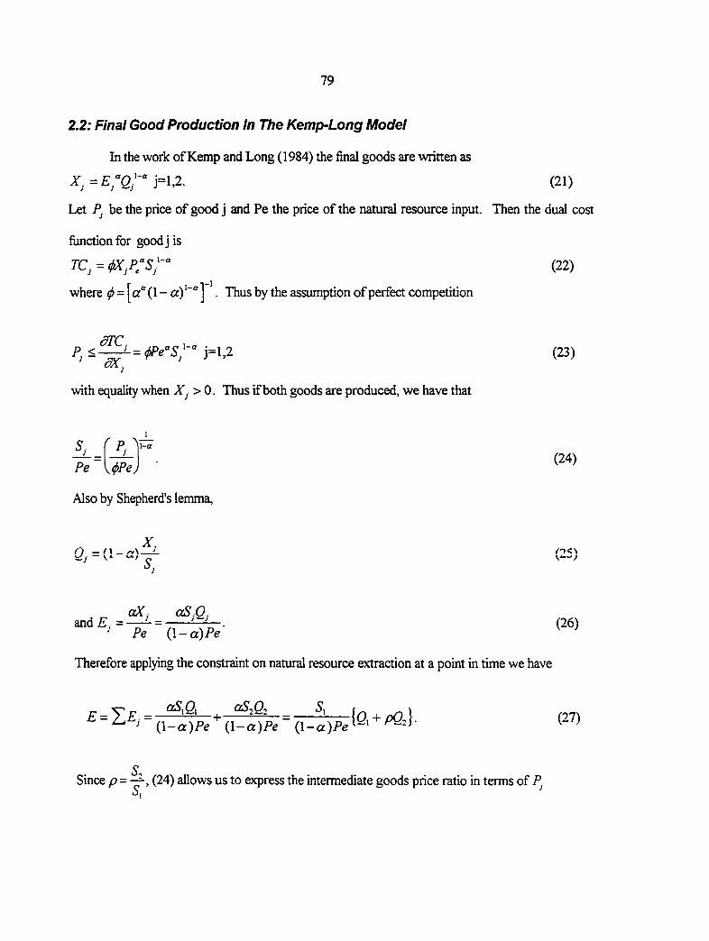
79
2.2; Final Good Production In The Kemp-Long Model
In the work of Kemp and Long (1984) the final goods are written as
X. =E;Q;-''ri,2. (21)
Let Pj be the price of good j and Pe the price of the natural resource input. Then the dual cost
function for good j is
TCj = (^jP/S/-" (22)
where ^ = [a" (1 - a)'"" ] '. Thus by the assumption of perfect competition
^rc P^<^=4Pe'^S;-'' j=l,2 (23)
with equality when > 0. Thus if both goods are produced, we have that
S ^ P^
Pe \.<j>Pej
Also by Shepherd's lemma.
(24)
O i. fn'^\ •^j — v o ^ '
aX, aS.O. and£,=—'- = (26)
' Pe {\-a)Pe ^ ^
Therefore applying the constrmnt on natural resource extraction at a point in time we have
(xS,0, (xS-,Q-t S, I \
^ " (l-a)Pe (l-a)Pe " (l-a)Pe^
5", Since P = -^, (24) allows us to express the intermediate goods price ratio in terms of P^
80
a constant (28)
As from (28) p is constant over time, the above analysis leads us to the foUowng conclusion.
Lemma (Kemp-Long (1984) lemma 3.1):
The competitive allocation of Ricardian factors is independent of the rate of natural resource
extraction.
^, = 0, ^2 > 0 when p>p^j \ Only final good 2 produced: Re^on HI
Again, as p, p^ and p^j are all fixed, (29) implies the following:
Proposition 1:
When the natural resource intensities are equal across the two goods (a, =«, = «) and extraction
is costless as in the Kemp-Long case, only two production patterns are possible: Either
(a) Only one and the same good is produced all the time or
(b) Both goods are produced all the time.
This is illustrated in Figure 2.2. In this case there is no change in production patterns over
time. Suppose that the prevailing parameters suggest that both goods be produced. Then the
theorems pertaining to static production patterns in the static trade model would hold here as well.
From (25) > 0 => Ej > 0 and = 0 => = 0 j=l,2. Thus
andO^ =0=>^, =0j=l,2.
Hence by (20) we conclude that
X, > 0, when p < : Only final good 1 produced: Regjon I
X, > 0, X^>0 when p e (p^ ,p^): Both final goods produced; Region n
(28b)
(29)
81
unaltered. In addition to production patterns an issue of interest is the rate of natural resource
extraction. Substituting for O, and (27) and simplifying we have
E = aLR{k + CO)
(1- a)Pe
However, from (6) we can substitute for R so that E can be expressed in terms of Pe alone.
(30)
E = E{Pe) = ocL{k-vcD)\(SJ9X^-\'
(l-a)/>.L(5^/0j'j
cd.{k+o))
{\-a)Pe L 5,"' J
ccL{k+(oi(SJ Pe)"" V"
(i-«)
aL{k-^co)
(1-a) y/^Pe ^r)
aL{k + CO) y/^
(l-a)Pe""-''> (31)
where = ¥i = ¥, (pj*)"
- and v's = ¥2 1/(^2-<>1) From this it follows that
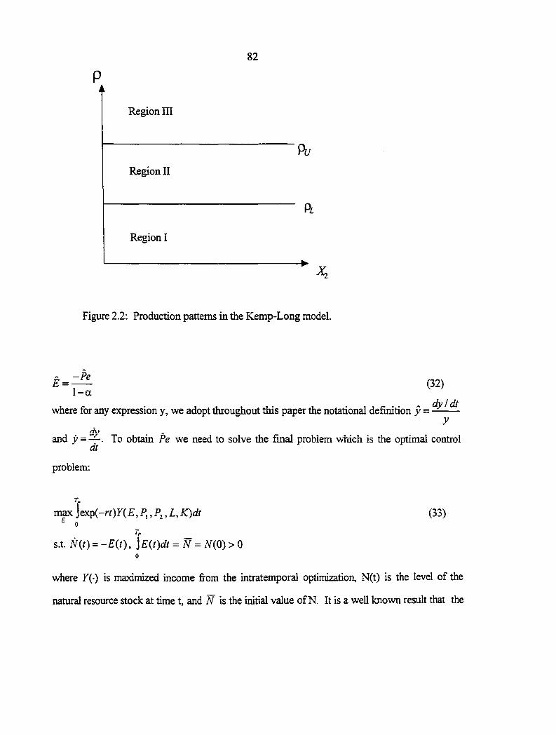
82
P • Region III
Region II
Hl
Region I
•
Figure 2.2: Production patterns in the Kemp-Long model.
- -Pe E = - (32)
1-a
where for any expression y, we adopt throughout this paper the notational definition y = y
dy and y = —. To obtain Pe we need to solve the final problem which is the optimal control
dt
problem;
max Jexp(-rr)F(£, P,, Pj, L, K)dt (33) ^ 0
jexp(-r 0
s.t. N{t) = -£(f), ]Eit )dt = N = N{Q) > 0 0
where K(-) is maximized income from the intratemporal optimization, N(t) is the level of the
natural resource stock at time t, and N is the initial value of N. It is a well known result that the
83
solution to this dynamic problem implies that the net shadow price of the resource rises at the rate
of interest. In the absence of extraction costs the net shadow price is equal to Pe. Thus, simply.
It follows then that
which was Lemma 3.2 of Kemp-Long. The rate of resource extraction is constant over time, E
declining at a rate faster than the rate of interest. Thus Kemp and Long established dynamic
counterparts of the four standard trade theorems. In the following section our first extension of the
Kemp-Long model is presented. We will allow for different natural resource intensities while
maintaining the assumption of costlessness of extraction.
2.3: Final Good Production With Different Resource Intensities
We introduce different natural resource intensities by allowing a, and to differ so that
now instead of (21) we have
Pe = r (34)
x.=E;^o;-''\i = \x (36)
As our dual cost functions we now have
TC^ = (37)
where (f)j = [(1 - )'"•' ] . Thus
p. =
when both goods are produced and hence
(38)
84
5, f P, y'"; Pe [<j>^Pe] •
The interaiediate good and natural resource input allocations are by Shephard's lemma.
J a Jf cCjSjOj
andE.=——- = —' ' ' . (41) ' Pe {\-aj)Pe ^ '
The above allows us to express the level of natural resource extraction in terms of the intermediate
good levels and prices and the natural resource price.
^ ' {\-a,)Pe (l-a,)Pe Pe\\-a, 1-a, J" ^ ^
As mentioned above the cone of diversification is fixed over time. Thus to investigate production
patterns we derive the path of p(t). By definition.
« i
5, SJPe [PJ<f,^Pef^- _ n = — = — = = = = = ^ " S, SJ Pe -±- f \—"
, r , a,-a, where J = j— and/?7 = = .
The path of the intermediate good price ratio is related to the path of the price of the natural
resource and is also influenced by final good prices through J which acts as a scaling factor. Thus,
unlike the Kemp-Long model the intermediate price ratio is no longer constant over time. Note
that the production rule (29) holds here as well. Taking logarithmic derivatives of (43) we have
p=J+mPe (44)
But by assumption J = 0. Therefore
85
p=mPe. (45)
Equation (45) provides some useful characterization;
Lemma 1:
When natural resource intensities differ, the ratio of intermediate good prices, p, varies J directly 1 {m>0o a^> aA i. , f with Pe over time as i „ r [inverselyJ < 0o a, < a,J
By similar reasoning as above a dual approach to our optimal control problem establishes
that Pe = r . This implies that
p = mr (46)
Thus we can establish a more specific characterization about p{t) than in lemma 1.
Lemma 2:
In the absence of extraction costs, when the natural resource intensities differ, the ratio of
intermediate good prices,
Jme5l f/n > 0 o a, > a, f over time as i .
{falls] [tw < 0 <» a, < a.
Thus by our variable definitions we can conclude the following;
Proposition 2;
Under the conditions of this model (specified in lemma 2), the price of the intermediate good used
in producing the more (less) resource intensive final good falls (rises) over time relative to the price
of the other intermediate good.
86
Now we are ready to investigate the nature of production patterns in this model. Since in
contrast to Kemp-Long, p is no longer constant over time, application of the rule in (29) leads us
to a conclusion regarding production patterns that is markedly different from that of Kemp-Long
(1984). Specifically, when different natural resource intensities are allowed in the GHOM,
production patterns could potentially go through three different stages: an initial stage in which
only one good is produced, a middle stage of changing shades of diversification during which both
goods are produced and a fiinal stage in which there is specialization in the good which was not
produced during the initial stage.
Figure 2.3 illustrates the two possible cases of production patterns over time. Which of the
two goods is produced at any stage depends on which one is more natural resource intensive.
Nonetheless, we can infer from Proposition 2 that in the region that occurs first, the more natural
resource intensive good is produced. Thus we can say the following;
Given the specifications of our model, there east potentially three stages of production: During
the initial stage if it occurs, there is specialization in the more natural resource intensive good. This
is followed by a second potential stage during which various shades of diversification occur. The
final stage will entail specialization in the good that is less natural resource intensive.
It is important to emphasize that the three-stage scenario of production pattems is only a
potential occurrence. Gven the initial conditions of the system with a, > a,, it is possible that
P<Pl never happen in which case Stage I will not occur. Similarly if p{Q) > p^ then there is
specialization in the good that is less natural resource intensive for all time.
In order to obtain a more specific characterization of production pattems we need to solve the
isoperimetric constraint. We will come to this issue later. Before then, we would like to
characterize the behavior of factor prices and the resource extraction profile. Totally differentiating
(7) and applying (46) we have
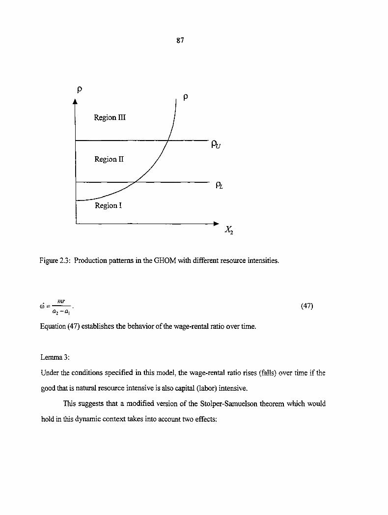
87
Region III
Region II
Region I
Figure 2.3: Production patterns in the GHOM with different resource intensities.
o5 = ^. (47)
Equation (47) establishes the behavior of the wage-rental ratio over time.
Lemma 3:
Under the conditions specified in this model, the wage-rental ratio rises (falls) over time if the
good that is natural resource intensive is also capital (labor) intensive.
This suggests that a modified version of the Stolper-Samuelson theorem which would
hold in this djmamic context takes into account two effects:
88
(a) the effect of a relative change in final good price, which is also considered in the static version
and the dynamic version analyzed by Kemp-Long, and
(b) the dynamic efifect of the rising level of the natural resource price.
Also of particular interest in the natural resource trade literature is the rate of natural
resource extraction. From (25) we can rewrite E as
E = {\-a,)Pe
Q\ + g,(I-gi)
a,(l-a,) pQi (48)
By an envelope theorem we know that
We also obtain by total differentiation of (39) that
(49)
Furthermore, define
Pej= 1,2. (50)
P . A J =1,2, (51) ^ dp X.
the elasticity of the jth intermediate good with respect to the intermediate good price ratio, p,
defined above. Then using (45), (49) and (50) we obtain upon total differentiation of (48):
£(/) = -Pe
(!-«,) + mPe pOj
a,( l-«i) . («i -<^2) mPe pOj
.a ,0-a,) ^a,( l-a ,) .
Q\ + PQi a,( l-a ,)
(52)
89
fnpQi = -Pe\
g,(gi-g,) g;(l-gi)
. cc,{\-a^)
0-ai) Q\-^ pQt
C^20•-C^^) .CjO-a^).
i.
Let us denote the expression in braces by /t: so that
E { t ) = - K P e i t ) . (53)
/tO By writing h = and by further simplifications we can rewrite ac in a more usefiil form;
Qi
1 ^ "zO-ai) " + b
K = -\ 1-a, a,(l-a2)
1 f,(a,-a,) —- + •
.1-a, a2(l-a,) (1-a,).
1 + ^ a;(l-ai)
a^0•-c^2)
(54)
Since > 0 we can show that K > 1
l-min(ai,a,) > 1 for every finite h. Furthermore it
1 olcr* /v i-T c (ry /v\>>/v/'l /v\ ^irV»<ar» V* 4 ^ *^-y \ ^ *^*7 J V * ] / ' ikAkWA AAAkA V WiJT ^ W AAWiA 1-a,
1 a, >a,, «•> if £,(a,-a,)>a,(l-a,). Thus we have that K is bounded below by
1-a,
[l-min(a,,a,)]"' . It can also be shown by some manipulation that K is bounded above if
max(ff,, £,) is finite. Recall that in the Kemp-Long case, k = 1 1 1
1-a, 1-a, 1-a Suppose
thai in the K-L case, a=a, ; then £, = -P^/(1-a,) and for a=a^\ then
£ = -.P^/(l-a,). Thus one would think that for a, a,,
E 6 (min(-.P^ /(l-a,),-P^ /(l-ci:,)),max(-.P^ /(l-a,),-P^ / (1-a,))) .
However, (53) and (54) show that this need not be the case. We can summarize these results in the
following proposition;
90
Proposition 3:
When the natural resource intensities differ across the two goods, the rate of natural resource
extraction is faster than that implied by the good with the lower resource intensity but it need not
be slower than that implied by the good with higher resource intensity. It could be faster than both.
This unexplained asymmetry means that the rate of natural resource extraction in this case
does not necessarily lie within the bounds implied by the two resource intensities even though this
might be what our intuition would suggest.
Corollary 3.1:
The rate of natural resource extraction is not an exogenously given constant. It is a funaion of the
ratio of the values of the intermediate goods (i)) and of the relative price elasticity of the
intermediate goods.
We can similarly obtain an expression for the level of resource extraction, E{t) as a
function of time and exogenous constants orJy. We start by substituting for O, and into (48)
and upon simplification we have
£ a,RL{X,k + ^co) (l-a,)(a,-a,)Pe
where A, = ^2giO-Q:2)-^iQ^20-Q^i) ^ (l-q,)g.(l-g,)-(l-a.)gi(l-g.)
Substituting for R and o) and bearing in mind that Pe = r -we obtain finally
91
cc E{t) = ^kPeiOy^ exp(Ti,rO + zPeCO)'^^ expCri^rr)
U ^ \ ) (56)
, ma, 1 m{\-a,) 1 where Ti, = ^ ' ^2 = = T1,+-
m
a^-^i 1-ct,
r = i ^'1'J e.
1_ -a.
1
u-a,
r , = '—, and jij = • V "2/'
a^-a, Oi-a,
Totally differentiating (56) we obtain an alternative expression for E which is useful for
comparing with the other extensions in this paper:
E=\—^ ^-^2
equation (106)
Applying the isoperimetric constraint
r where vi;,,vj;2, ^o jij are defined in the general case following
l£:(0^^/ = A^ = ^(0)>0 (57)
one gets
-rr -<X LT J XkPejOf' ^ ^2-^^(0)"'
It is not possible to solve (58) explicitly for a closed-form expression for Pe(0). However,
one can simulate the above expression to obtain the locus of Pe(0) over the parameter space. The
value of P,(0) for any given parameter realization can be used to infer production patterns as
92
follows. We know from above that at any time t, only good 1 is produced if /?(/) < both if
p{t) e and only good 2 if pit)> p^. Since p{t) = JPei^y tx'pimrt) we have
p{0) = JPeiOy and piT) = JPe(0)"' exp{mrT). Assume without loss of generality that m>0.
Then p(t) rises over time. If p(0) < p^ and p{T)> p^ then by continuity of p(/) all three
stages occur. In terms of the initial price of the natural resource
P(0)<Pi =>^e(0)<" a.k J '
T J J
Mm
= P and
PiT)> Pu =>P,(0)>-a^k
,1-a.
9. ,^,Jexp(/nrr).
= P.
So all three stages occur if P^^ < P^(0) < P^^. Furthermore define
ajc f ^2 1 Ll-a,. ^9jJ exTp{mrT)^
l /m
' and
p: =
1 1 Mm
It is clear that < P^^ < and that < P^^ < PJ^. Also for some general parameter values,
< P^^ < P^^ < -^4 • ^ following proposition.
93
Proposition 4:
Under suitable parameter scenarios in the GHOM with different natural resource intensities,
alternative production patterns result depending on the initial level of the natural resource price as
follows:
(a) If P,(0) < there will be specialization in the natural resource intensive good
(b) If P,(0) 6 ) there will be specialization in the natural resource intensive good followed
by diversification.
(c) If P^(0) e there will be specialization in the natural resource intensive good initially,
followed by a period of diversification and finally specialization in the other good.
(d) If P^(0) s (P^^,PJ^) there will be diversification initially followed by specialization in the
natural resource unintensive good.
(e) If P,(0) > PJ^ there will be specialization in the natural resource unintensive good.
Proof
Recall that without loss of generality, good 1 is relatively natural resource intensive.
P few P' c" T\ n TViic nnUr rorrtr^n \ r^\^/ ^ A-'v / ^ r^L'
(b) P^(0) € (P/. ,Pe^) o piT) py) and p{0) < p^. Thus regions 1 and then 2 occur.
(c) P^(0) e (P^^,P^^.) o p(0) < and p{T)> p^. So we have regions 1 then 2 and then 3.
(d) P^(0) s{P^^,Pj^)o p(0) g(p^,P jj) and p{T)> p^. Thisgves us regions 2 and then 3.
(e) P^(0) > PJ o p(T)> p(0) > Pu. Only region 3 occurs.
The above model can be simulated to infer production patterns over various parameter
realizations. Simulation results have not been reported in this paper. The locus of Pe(0) implies
also a locus for p(0) = JPeiJS)'" over the parameter space. We can also derive an analytical
expression for the period of diversification that does not depend on the solution value of Pe(0) but

94
rather depends on p^j Ip^, the ratio of the limits of the cone of diversification. Let a superscript
denote the solution values based on (58) so that Pe(0)* is the value of Pe(0) that solves (58).
Then p(0)* = JPe(Qi)*'" or p{t)* = JPe{0)''" exp(/wrt). Assume without loss of generality that
a, > • Suppose fiirther that all stages occur. In that case /, is the time of transition fi-om Stage
I to Stage n, where r, solves
Pj^ = JPeiO)'" exp(/nr/i). (59)
Similarly, is the time of transition fi-om Stage II to Stage HI, where /, solves
Py = JPeiO)*" exp {mrt^_). (60)
Solving (59) and (60) for /, and U respectively we obtain
t =—In mr
PL \JPeiSS)'"
and (61)
^2 = 1
In mr
PU UPe(O)*''
Thus it is clear that for a, >a^m>0 and since p^ > we will have < /,.
Subtractine Coi") from (62) we have the period of diversification to be
(62)
1 U-t, =—In
mr
r \ Bm. (63)
The results of this section, in particular Corollary 3.1, imply that a country that is capital
(labor) rich may not speciaUze in the capital (labor) intensive good ail the time. Suppose the
country concerned is capital rich and the capital intensive good is the less natural resource
intensive, say good 2 in our model. Suppose further that p(0), the initial value of the intermediate
good price ratio is low enough so that all three phases of production patterns occur. Then
according to Corollary 3.1, this country will specialize in the labor intensive good until time
95
when it will begin a phase of diversification. At a later time this country will finally move into
specialization in the capital rich good. The feet that this country is capital rich means that and U
vwU be smaller than if it were not, but firom (63) the period of diversification will not be affected.
2.4; Summary
In this section of the paper we extended the GHOM of Kemp and Long (1984) to allow
for different natural resource intensities. A dual approach was used which simplified the analysis
substantially. The results indicate that unlike the Kemp-Long case there is no trivial steady state in
this model. There are three potential regions of production. If the initial stage occurs, this will
entail specialization in the more natural resource intensive good. This will be followed by a stage
of varying shades of diversification. Increasing shares of income will be attributed to the
production of the less natural resource intensive good as the intermediate good price ratios rises
through the cone of diversification. The cone of diversification is fixed through time. The final
stage will be characterized by specialization in the less natural resource intensive good.
The results of this section may very well explain at least in part, the decline in the share of
agriculture and other primary industries in the gross domestic product of most countries. Though
this decline has been attributed to other factors in the grovrth literature, our results are not
dependent upon the stage of development of a country. We find that, especially for natural
resource rich countries, a decline in the share of natural resource intensive industries in GDP is
expected over time as the resource base of the country declines. A necessary caveat here is that the
presence of backstops may make it hard to verify empirically.
Given the above results, a capital rich country need not export or even produce the more
capital intensive good ever, or at least not always, nor does a labor rich countiy, the labor intensive
good. It is usefial to emphasize that the three phases of production patterns suggested here are
96
potential and do not all have to occur. The actual pattern depends on the set of parameters
prevailing. These results may help explain the Leontief paradox and other puzzling empirical
observations about the static trade theorems. If preferences are identical across countries, as
assumed in the H-0 model, then these production patterns also imply trade patterns.
97
3: THE GHOM WITH EQUAL NATURAL RESOURCE INTENSITIES AND POSITIVE MARGINAL EXTRACTION COSTS
In this section we introduce a different extension to the Kemp-Long model. We revert to
the assumption of equal resource intensities but now allow for positive mar^al costs of extraction.
We employ the same dual approach that we used in previous sections.
In a similar extension applied to the hybrid model of Kemp-Long, Ono (1982) showed that
when positive mar^nal extraction costs are allowed, no trivial steady state ensues; rather there is
necessarily a transition from one mode of specialization through a period of diversification to the
opposite mode of specialization. In accordance with Ono's results we show in this section that
after allowing for positive marginal extraction costs of the Cobb-Douglas form of technology in the
GHOM of Kemp-Long, the results of their model are not upheld. Introducing extraction costs of
the Cobb-Douglas form results in a cone of diversification that changes over time. The assumption
of equal natural resource intensities means that unlike the previous section, the intermediate good
price is constant over time. However, the dynamic nature of the cone of diversification leads to
scenarios of production patterns similar to what we saw in the previous section
3.1: Intermediate Good Production
The production fiinction for the intermediate goods is still the same as in section 2.1:
The dual cost function is /-* n TTr^i
where Bj = (1 j .
98
W = (0, /S,}
1-a,
andi?= — Hs,/e,y'
J 02-01
The allocations of labor and capital in producing 0, and are again
(Lfm. ' fV ' R
Now suppose that the natural resource input is extracted using labor and capital inputs.
Suppose further that this extraction fiinction is also of Cobb-Douglas form so that
E = G(,L,,K,) = V ^3 e(0,l) (64)
Thus the dual cost function for resource extraction is
C3 = e^EW'R}-"'. (65)
where 6^ = (1 - fits )^'''''^ j . Thus we have
7= ,-^=0W'''R'-''K cE '
Therefore
(66)
i , = ^ ^ a n d JV
(67)
^3 = R
Our resource constraints now take the form
AO = B,
(68)
(69)
where A and Q are as before and 5, =
Thus 0 = A'^B, and hence we obtain
RK-i\-a,)T]E
WL-a,T]E
99
_a,[RK-{\-a,)TiE]-{ \ -a,){WL-a,r]E] and (70)
(1 - a, - AjT/E] - or, [i?Ar - (1 -(71)
Tt E Using the definitions of o), k, and p and also defining r = — and e = —, we may write
W L
Q _ RL {a.k - [(1 - a,) + (a, - ) ze]6j}
(aj-a,)^, (72)
a = /?Z,{[(l-a,)+ ze(a, -a^)\a}-a^k}
(^2 )'^2
Thus by similar manipulations as in the previous section we may conclude that
Q > 0, 02 = 0 when p<pl : Only good 1 produced; Region I
Q, > 0, ^2 > 0 when p^ipi ,p^ ): Both goods produced; Region II
O, = 0, Qj > 0 when p'>p^ ; Only good 2 produced; Region III
where
(73)
(74)
PL = _(\-a,) + {a^-a^)re\ a^k
(75)
Pu = ajc
(^^n \4-(n —n Y"(e^
o J-V ' v^2 (76)
and again pl < p^' when a, a, • Th® cone of diversification is (pl ,p^'). Note that pl and '
are fianctions of ze which in general changes over time. Therefore we may make the following
observation;
100
Lemma 4:
In the GHOM where natural resovirce intensities differ and there are positive marginal costs of
extraction, the interval of diversification in general is not fixed over time but has the tendency
to change.
Lemma 5:
Under the conditions specified in this model the interval of diversification is fixed over time if
and only if the cost of resource extraction and returns to the labor endowment are in constant
proportion over time.
Proof:
First note from equations and that pj^' and Py' are both constant if and only if ze is constant Tj 7
(re = 0). Then by definition e = —— and hence p^' and py' are both constant if and only if rr jU
ti£ = cfVL where c is a constant.
As we shall find out in the next subsection, with equal natural resource intensities, CO is
constant over time. Hence X is also constant over time because it is a fimction of CO only.
3.2: Final Good Production
The final goods are produced according to the specifications of the Kemp-Long model,
outlined in Section 2.2;
X^ = E;QjiL^.K^y-\ i=\ ,2.
Thus we have
P = $2 S^/Pe [P^/^Pe] 1-a /
S. SJ Pe ^ ^ ^ ^ P. l-a
a constant.
101
Now since p is constant any transitions in production patterns must result from changes
in the boundaries of the interval of diversification. The only expression in p^' and p^;' that may
have a tendency to change over tune is xe, the ratio of the cost of natural resource extraction as
compared to the retums to labor. That p is constant implies also that CO is constant over time
provided that final goods prices remain unchanged. We investigate production pattems in a
manner similar to the previous section. Here we first obtain an expression for E{t). From
above we have
(l-a)Pe
Substituting for 0, and from Section 3.1 we get
O.LR a2k-(£>[{[-a2) + {a2 -a3)Te]+co[(l-a,)+(fl, -a yie]-a k (77)
upon simplification. Collecting like terms together we finally have
where jiq =a.{a^-a^) I ii; = - 0^"'
p ' ^ 1 , = ( a , J " , / ( " - : )
\ (p /
f p \l/(l-a ) '0 2°'
r = and vj •, = 1 - a
102
Applying the isoperimetric constraint one can solve numerically for Pj(0). Totally
differentiating the expression for £(/) we obtain
E = Hz
Again, since p is constant we have that & = 0 which means W=R. Hence from the natural
resource extraction technology, tj=W= R. Furthermore, since
1 l-flt
(78)
(79)
(80)
Pe l(pPe_
as in equation (24) we have
£2Pe+(l-a)[a,fr+(l-a,)^] = = 0
c^*e + {\- a)[a^W•^{\-a^)R\ = P, =0
Thus
P e = — = a a
Now it is important to note that when we allow for extraction costs, the net shadow value
of the natural resource, which we will represent by X, is not equal to the gross value, P^.
Specif ical ly , a = Pe- t j
so that - n ^ X -1 T] ^ Xr Pe = — T}+—X = — n+—.
Pe Pe Pe Pe
Thn^ tnopthpr with tKic cn\rAC nc tho fXllrvunnrr --'O V"-"-/ — ^ *.AAW
-iPe-T])ra « . ^ fr = = R=t j and
r j a + { l - a ) P e (81)
103
Pe = {\-a){Pe-Ti)r Tja+(\-a)Pe
Thus from (80)
(82)
E = { \ -a){P,-n)r
- M s - M i P e " " J + i ^ - a ) P ,
(83)
Equation (83) leads us to the following conclusion.
Proposition 5:
The rate of natural resource extraction is not constant. It depends on the values of Pe, the resource
price and 7, the marginal cost of extraction.
The time derivatives of the factor prices also imply the following.
Proposition 6;
Given the assumptions of our model the price of the natural resource rises over time while the
prices of the Ricardian factors and the marginal cost of extraction all fall over time at the same
increasing rate.
The possible patterns of production are illustrated in Figures 3.1 through 3.5. As
mentioned earlier, since p is constant, production patterns are determined by the paths of
p[ and pIj relative to the constant value of p.
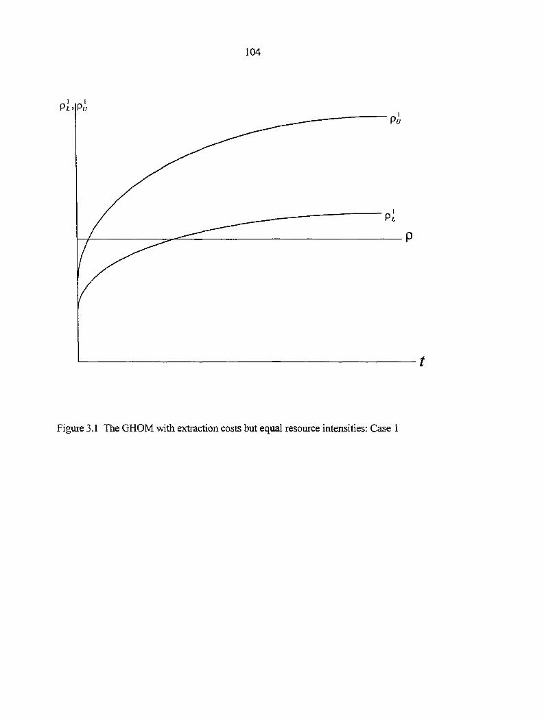
104
Figure 3.1 The GHOM with extraction costs but equal resource intensities: Case 1

105
Figure 3.2 The GHOM with extraction costs but equal resource intensities: Case 2.
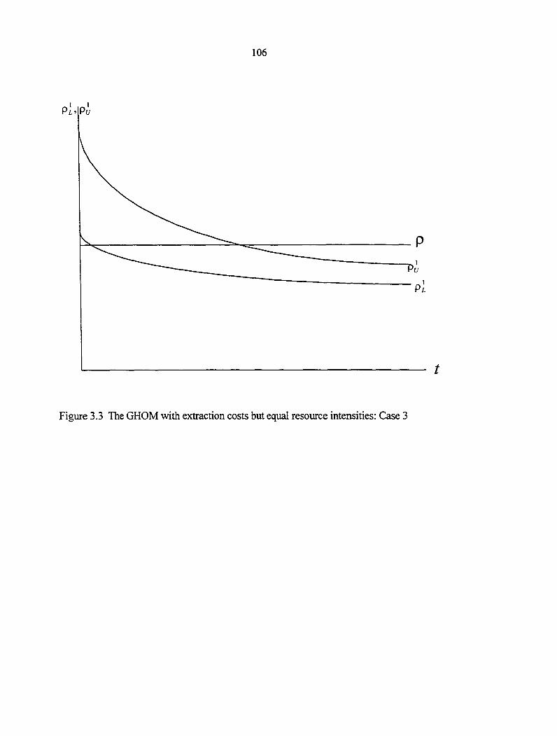
106
Figure 3.3 The GHOM with extraction costs but equal resource intensities: Case 3
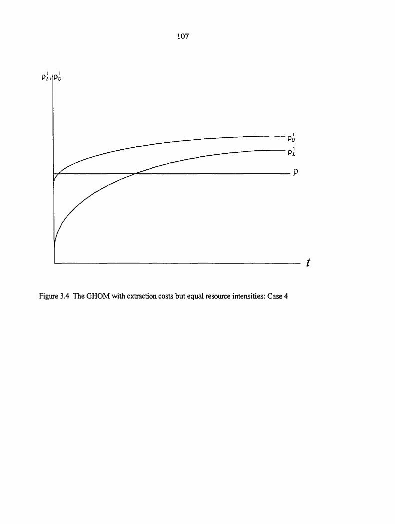
107
Figure 3.4 The GHOM with extraction costs but equal resource intensities: Case 4
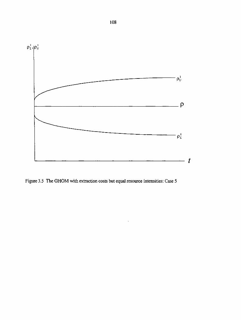
108
Figure 3.5 The GHOM with extraction costs but equal resource intensities: Case 5
109
3.3: Summary
The present section of this paper maintained the Kemp-Long assumption of equal resource
intensities but allowed for positive marginal extraction costs. The analysis indicates that when
positive marginal extraction costs are allowed in the Kemp-Long model their results are not
upheld. Rather we find that three potential phases of production may occur. In the initial phase
one of the goods may be produced alone. An intermediate phase of diversification is possible
which may be followed by a final phase of speciali2a,tion in the other good. This result is similar to
the findings of Ono (1982) whose analysis was performed in a two good, two input model.
Furthermore Ono's results in the context of the hybrid model. He concluded that when nontrivial
extraction costs are allowed there is a transition in the production scenarios fi^om specialization in
the more natural resource intensive good through various shades of diversification to specialization
in the less natural resource good. In this section allowing for positive marginal extraction costs
leads to a dynamic cone of diversification so that alternative production patterns result even though
the intermediate goods price ratio was constant over time.
110
4: THE GHOM WITH DIFFERENT NATURAL RESOURCE INTENSITIES AND POSITIVE EXTRACTION COSTS
In this section we introduce the most general extension of the GHOM of Kemp-Long by
combining the extensions of the previous sections. In section 2 we allowed for different natural
resource intensities across the two sectors but maintained the assumption that the raw material is
obtained costlessly from a ^ven natural resource stock. In section 3 we introduced positive
marginal extraction costs but maintained the Kemp-Long assumption of equal natural resource
intensities. We will now allow for positive marginal costs of extraction and different natural
resource intensities and see what implications this has for production patterns. As Ono (1982)
pointed out, simply allowing for positive costs of extraction is not enough since positive but
constant costs of extraction would yield the same results as in the case of zero extraction costs.
That natural resource extraction is a costly process is generally the rule rather than the
exception. Allowng for this then together with different resource intensities would help us to more
closely represent the issues that are considered in optimal decision making especially in a natural
resource rich country. Ono (1982) allowed for positive mar^nal extraction costs in a two good -
two factor model and realized a sigmficant departure from the results of the two good - t^.vo factor
zero extraction costs model. This was the hybrid model of Kemp-Long (1979). Whereas in the
zero costs model of Kemp-Long (1979) a competitive economy always specializes in production,
with positive marginal costs of extraction there is a transition from one mode of specialization
through diversification to the opposite mode of specialization, the more natural resource intensive
good being produced first.
4.1: Intermediate Good Production
The production of the intermediate good takes the same form as in sections 2.1;
Oj = .
I l l
Furthermore, labor and capital inputs are used in the extraction of the natural resource according
to equation (64) in Section 3.1:
Thus all the results in Section 3.1 hold here as well. In particular the two intermediate goods are
Q ^ -aJ[co-a,k} (a,-a,)5,
which are equations (71) and (72). The cone of diversification, (p^' ,/7y'), has the same form as in
equations (74) and (75) of Section 3.1. However, we shall see that they do not hold in exactly the
same way.
4.2: Final Good Production
We will now turn to the production of the final good. Tne treatment here is much the same
as in Section 2 and so equations (36) through (45) hold here as well except that and ' would
replace and p^ respectively. Thus corresponding to equation (29) we have
O, = 0, 02 > 0 o A', = 0, A', > 0 <=> p>pu
Lemma 1 also holds here. Furthermore the dual version of the optimal control problem suggests
that the net shadow value of the natural resource rises at the rate of interest. Hence as in the
pre\aous sections we have
E = G{L„K,) = K;-'-^L,'-' a, (0,1)
given as
Q > 0, 02 = 0 o A", > 0, Xj = 0 p<pI
G 02 >0 o X, >0, A', >0 o pe(p/,py') (84)
A = Pe- T] (85)
112
where rj is the marginal cx)st of extraction. The results obtained in the previous section were based
on the assumption that rj=0 so that A = Pe whence X = r = Pe. Now we have by differentiating
(85) that
A Tj ^ A '1 T} ^ Ar Pe = -^7+—;i = -^7+—. (86)
Pe Pe Pe Pe
The rate of change of the resource price is a weighted average of the rate of change of the
marginal cost of extraction and that of the net shadow value of the resource. Thus if P^ rises
slower than r it would mean that r] rises slower than P^ and conversely. More specifically,
P^ e (min(77,r),max(;7,r))
From (66) we know that
T]=a^+{\-a^)R. (87)
Taking logarithmic derivatives of equation (38) we have
a,Pe + (l-a,)5, =0 (88)
a^Pe + (1 - 0^)5, = P, = 0. (89) S
Also fi^om previous expressions for R and W and becausep = — we can write the following; 5;
5, - 5, = mPe = (^2 - or, )[W - .R] (90)
= (91)
R = (92)
- (l-o,)5,-(l-a,)5, ir=- ' - (93)
a, -o,
Equations (90) through (93) and either of equations (88) or (89) form a five equation which can be
solved for Pe, R, W. We first obtain Pe as
113
- rX Pe = —
7
a .1-a,
, (a,-a.)m Pe +—' —
a. 7 J
•I f -r — - 1
A
a, (a, -a^)m Pe
Ll-a, a,-a, 7 J (94)
Further simplification yields
Pe = r{Pe-rT) [Pe+Sr})
(95)
where 5=+ 1-a, ^2~^l ^"^2 ^2~^!
Thus by substitution we have
/w(l-a,) a,
_ - a, •(P^-77)
. o-' -o. -S iPe- T ] )
{Pe + 5r]) {Pe + Srj) (96)
r a,/w or, ; I 1 r in re — n I 1 \ 1 • I I T%
R = La,-a, l-a,J^ " la,-a.
-o r\ re —v\
[Pe + dT]) [Pe + 5ri) (97)
e -giKPg-T?)
' (l-a,)(Pe + ;7) ^ (98)
5,=- -«,/•( Pe-77)
(l-aj)(Pe + 57)
Also applying equation (45) we get
(99)
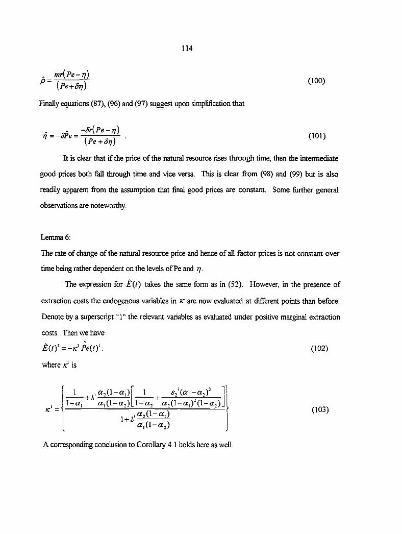
114
. mr[Pe-Tj)
{Pe-¥5ri) (100)
Finally equations (87), (96) and (97) suggest upon simplification that
(101)
It is clear that if the price of the natural resource rises through time, then the intermediate
good prices both fall through time and \dce versa. This is clear from (98) and (99) but is also
readily apparent from the assumption that final good prices are constant. Some fiarther general
observations are noteworthy.
Lemma 6:
The rate of change of the natural resource price and hence of all factor prices is not constant over
time being rather dependent on the levels of Pe and rj.
The expression for £,(t) takes the same form as in (52). However, in the presence of
extraction costs the endogenous variables in k are now evaluated at different points than before.
Denote by a superscript "1" the relevant variables as evaluated under positive mar^nal extraction
costs. Then we have
^(t)' =-K^ Pe{t)\
where is
(102)
1 Q;,(l-gi) 1 g;'(Qri -a^Y
(103)
1 + cTiCl-a,)
A corresponding conclusion to Corollary 4.1 holds here as well.
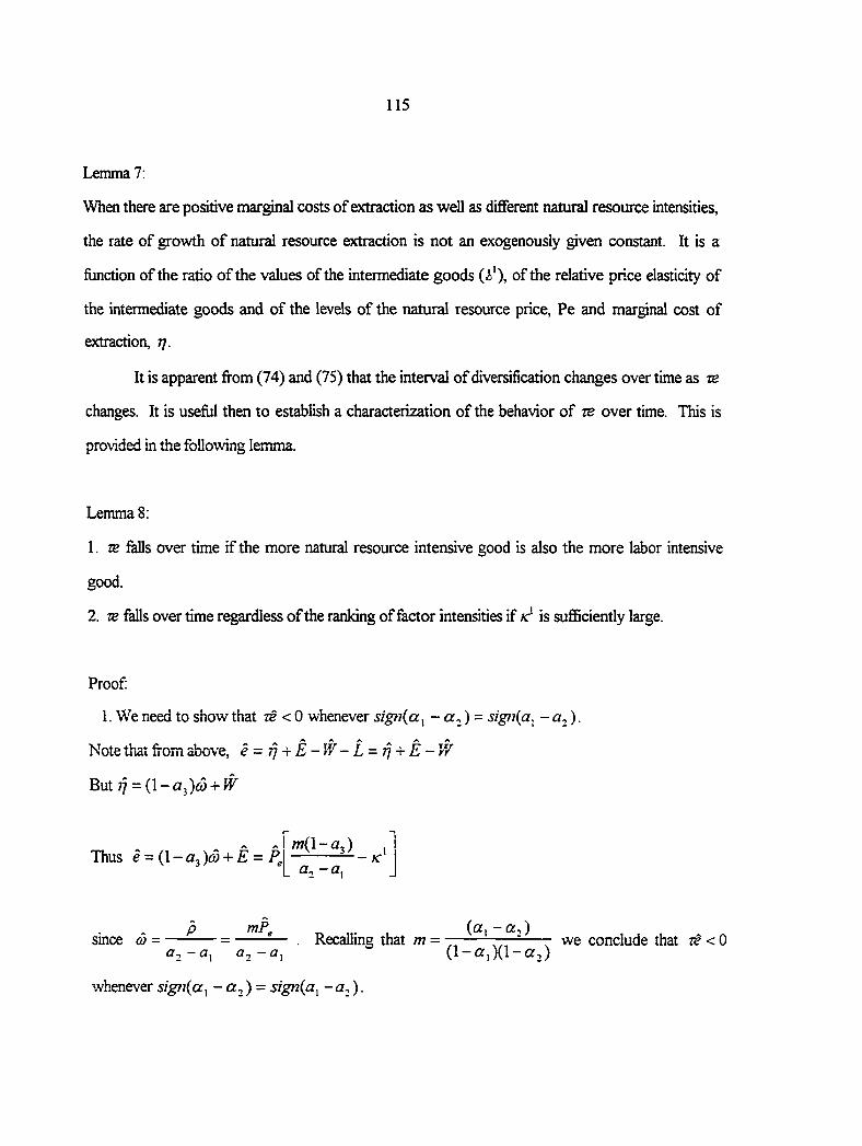
115
Lemma?:
When there are positive marginal costs of extraction as well as different natural resource intensities,
the rate of growth of natural resource extraction is not an exogenously g?ven constant. It is a
fimction of the ratio of the values of the intermediate goods (i'), of the relative price elasticity of
the intermediate goods and of the levels of the natural resource price, Pe and mar^nal cost of
extraction, ?].
It is apparent from (74) and (75) that the interval of diversification changes over time as zb
changes. It is useful then to establish a characterization of the behavior of ze over time. This is
provided in the following lemma.
Lemma 8;
1. ze falls over time if the more natural resource intensive good is also the more labor intensive
good.
2. ze falls over time regardless of the ranking of factor intensities if is sufiSciently large.
Proof
1. We need to show that re <0 whenever sigfi{a^ - ) = sign{a^ -<^2)-
Note that from above, e = + E - W - L = t] + E - W
But i] = (1-0^)65 +
Cl 'y flfi - IC
since CO = P mP^ Recalling that m =
(g| -g;) we conclude that re <Q
C I ^ (l-a,)(l-a,)
whenever 5/g7/(a, - a,) = 5/gn(flr, -a,).
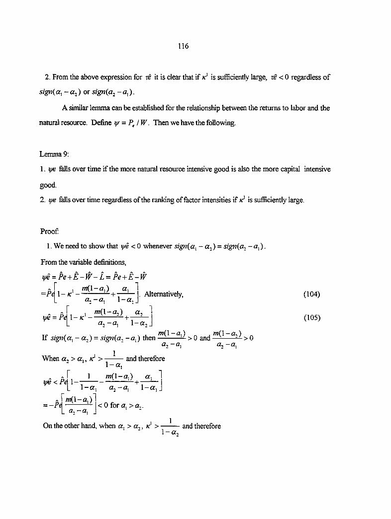
116
2. From the above expression for xe it is clear that if is sufficiently large, ze < 0 regardless of
sign{a^ - ) or sign(a^ - a,).
A similar lemma can be established for the relationship between the returns to labor and the
natural resource. Define y/ = P^IW. Then we have the following.
Lemma 9:
1. y/e falls over time if the more natural resource intensive good is also the more capital intensive
good.
2. m falls over time regardless of the ranking of factor intensities if /c" is sufficiently large.
Proof:
1. We need to show that y/e <0 whenever sign{a^ - a,) = sigtiia^ - ) •
From the variable definitions,
y/e = Pe + E-W-L = Pe + E-W
=Pd 1 nt{\-a,) g,
1-a. . Alternatively,
y/e = Pe 1 - v ' a.
+ -
a, - a, 1-a,
Tf. . / s . / s . r. ,OT(l-<ar,) „ If sign(a^ ~ <^2) = ~0 0
a, -a, a, -a, 1
When a, > a,, /c' > and therefore 1-a,
1 m(\-a.^ a. y / e < P d 1 - ^ — ^ — +
= -Pd
L 1-a, l-«i
a, -a 1 -I < 0 for a. >a,.
On the other hand, when a, > a,, /c' > 1-a.,
and therefore
(104)
(105)
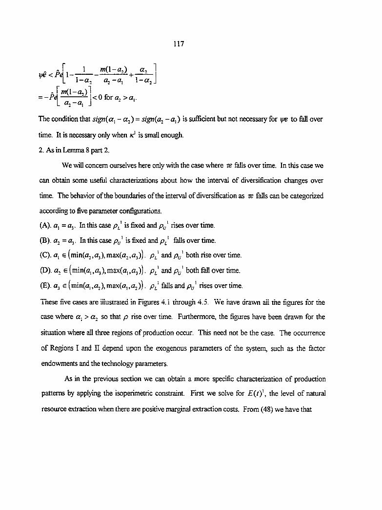
117
if/e <Pe
= -Pe
1 m(l-a,) a, 1 _ - ~-+-
1-a, 02~'^X 1~®2J
a,-a, J <0 fora, >a,.
The condition that sign(a^ ~ 2)- •^'^('^2 ~<^i) suflBcient but not necessary for y/e to fall over
time. It is necessary only when is small enough.
2. As in Lemma 8 part 2.
We will concern ourselves here only wth the case where tb falls over time. In this case we
can obtain some usefiil characterizations about how the interval of diversification changes over
time. The behavior of the boundaries of the interval of diversification as re falls can be categorized
according to five parameter configurations.
(A), a, = flj. In this case is fixed and rises over time.
(B). ^2=03. In this case Py is fixed and falls over time.
(C). e (min(a2,a3),max(a,,a3)). and Py' both rise overtime.
(D). a, e (min(a,,a3),max(a,,a3)). and both fall over time.
(E). 6 (min(a,,a,),max(<ar,,a,)). Pj,' falls and Py rises overtime.
Tnese five cases are iilustraied in Figures 4.1 through 4.5. We have drawn aii the figures for the
case where <2, > or, so that p rise over time. Furthermore, the figures have been drawn for the
situation where all three regions of production occur. This need not be the case. The occurrence
of Regions I and n depend upon the exogenous parameters of the system, such as the factor
endowments and the technology parameters.
As in the previous section we can obtain a more specific characterization of production
patterns by applying the isoperimetric constraint. First we solve for E(t)\ the level of natural
resource extraction when there are positive marginal extraction costs. From (48) we have that
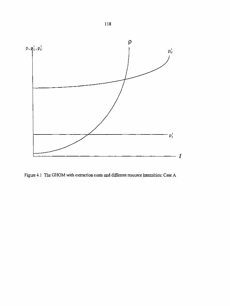
118
P
Figure 4.1 The GHOM with extraction costs and different resource intensities: Case A
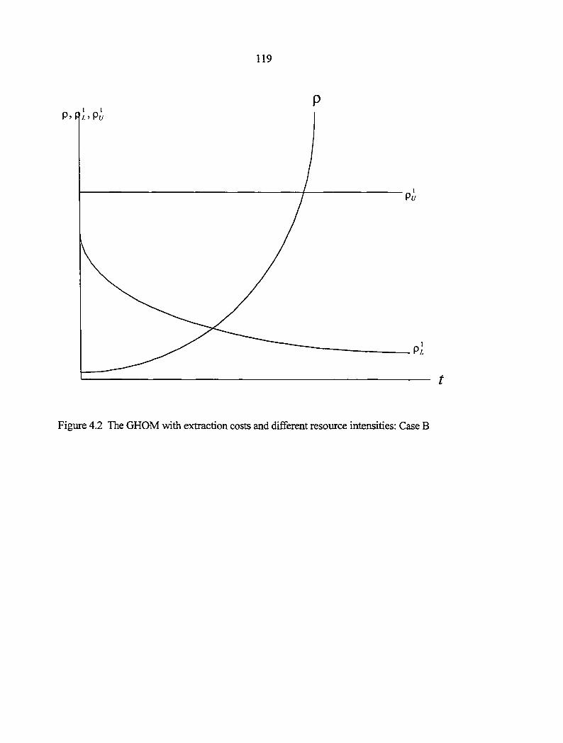
119
Figure 4.2 The GHOM with extraction costs and different resource intensities: Case B
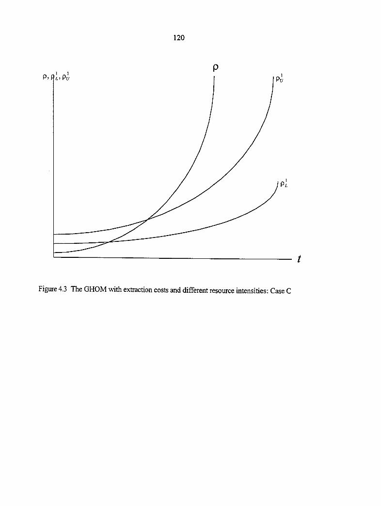
120
Figure 4.3 The GHOM with extraction costs and different resource intensities: Case C
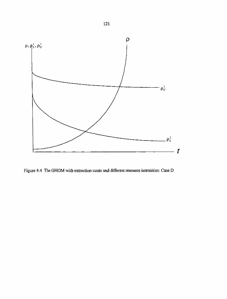
121
Figure 4.4 The GHOM with extraction costs and different resource intensities: Case D
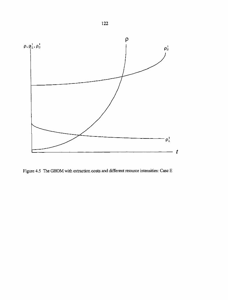
122
Figure 4.5 The GHOM with extraction costs and different resource intensities: Case E
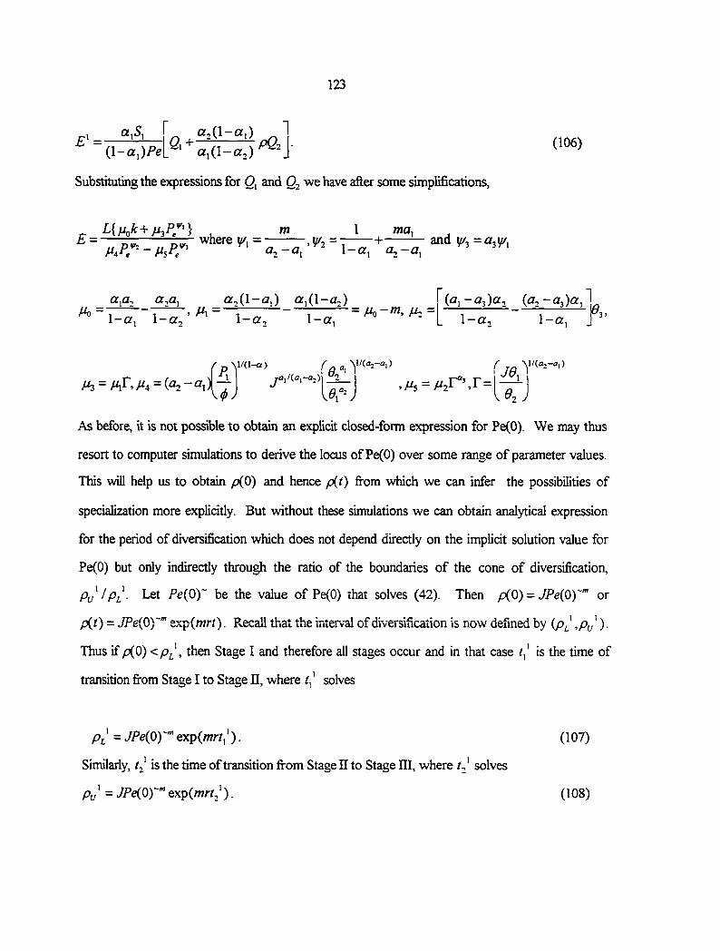
123
£' = (l-a,)Pe
g^O-Qi)
aiO-ttz) P02 (106)
Substituting the expressions for 0, and Oj we have after some simplifications,
^ LiMok+M^P/'} . /w E = —rT: TTT" where y/^ =
M.P:- - MsPe Vj a,-a, ,¥2 =
1 ma.
1-a, and =<3f3^i
a,a, a,a,
1-a, 1-a,''"' 1~Q^2
a;(l-(Ji) ai(l-a;)
1-a, • = Mz =
(a,-a^)a. {a.-a,)a, 1-a, 1-a, P.,
^ = Ma = (.02-^1) ^ y/d-a)
M ya,/(a,-a,) ,/^5 = i"2r°'.r=
Y/(a:-a,)
As before, it is not possible to obtain an explicit closed-form expression for Pe(0). We may thus
resort to computer simulations to derive the locus of Pe(0) over some range of parameter values.
This will help us to obtain /c»(0) and hence p(t) fi"om which we can infer the possibilities of
specialization more explicitly. But without these simulations we can obtain analytical expression
for the period of diversification which does not depend directly on the implicit solution value for
Pe(0) but only indirectly through the ratio of the boundaries of the cone of diversification,
Py I Pi. Let Pe{Q)~ be the value of Pe(0) that solves (42). Then p(0) = JPeiOy" or
p(0 = JPeiOy" exp(mrr). Recall that the interval of diversification is now defined by (p^' ,Pu)-
Thus if p(0) <p^', then Stage I and therefore all stages occur and in that case is the time of
transition firom Stage I to Stage n, where solves
Pi = JPeiO)"" exp(/wrt,').
Similarly, ij is the time of transition from Stage 11 to Stage HI, where solves
Pfj^ = JPeiOy" exp(Anrt,').
(107)
(108)

124
Solving and for and respectively we obtain
=—In mr
PL JPeioy
and (109)
=—In mr
« 1 ^ Pu
vype(o)~'
Thus we finally have the period of diversification to be
(110)
ln| mr
Pu
\.Pl J /I 1 1 \ viil)
4.3: Summary
In addition to allo\\dng for different natural resource intensities this section of the model
extended the GHOM of Kemp and Long (1984) to permit positive marginal costs of extraction.
The extraction technclog>' was represented by a Cobb-Douglas production function in which labor
and capital are employed as inputs to aid in the extraction process. The resuhs indicate that the
intermediate price ratio as well as the cone of diversification change over time. As in the previous
section there are three potential stages of production. If the initial value of the intermediate price
ratio is small enough and the time horizon is long enough all three stages will occur. In that case
the initial stage will be characterized by specialization in the natural resource intensive good. This
will be followed by a stage of varying shades of diversification and finally by a period of
specialization in the less natural resource intensive good. As in the previous section the rate of
extraction of the resource is a fijnction of time. In addition the rate of growth of the price of the
resource is also a function of time. We find that when the resource intensive good is also capital
125
intensive the returns to the natural resource falls relative to the returns to labor. We restriaed
ourselves to the case where the cost of natural resource was also falling relative to the returns to
labor. Five general types of dynamic implications of the changes in the cone of diversification and
the intermediate good price ratio were identified based on corresponding parameter configurations.
In at least three of these it is clear that the cone of diversification widens over time. The major
implications of positive mar^nal extraction costs as opposed to the previous section are with
regard to the timing of the transitions fi'om one stage to another.
126
5: CONCLUSION In this paper we considered the dynamic issues of natural resource-trade models within the
context of the GHOM of Kemp-Long. We extended their model to account for different natural
resource intensities and positive mar^nal extraction costs. In the first part we considered different
natural resource intensities but maintained zero costs of extraction. In the second part we allowed
for positive marginal extraction costs but maintained equal resource intensities. Finally, in the last
part we combined the first two extensions by allowing for positive marginal extraction costs and
different natural resource intensities. Various propositions that differed from the Kemp-Long
conclusions were established.
The implication of different natural resource intensities is that the intermediate good price
ratio takes on a dynamic nature, with a path that depends on the time profile of the price of the
resource. On the other hand when positive marginal extraction costs are introduced, the cone of
diversification is no longer static but dynamic with a path determined in part by the path of resource
extraction and in part also by the path of the wage rental ratio. .Aii the thxee models considered
here suggest that no definite production pattern exists for all parameter realizations. A brief
summary of the results of these models is given in Table 1. The likely production pattern for any
gjven country is an issue that can only be resolved empirically. However, simulation results
provide insights into how thcss patterns chsngc with ccrtsin ksy psrsmstcrs such ^ Isngtli of tims
horizon, rate of interest and initial stock of natural resource.
One important implication of these results is that a country endowed in a given resource
need not export or even produce the good relatively intensive in that resource all the time. This
127
may help explain the occurrence of the Leontief paradox. When natural resource inputs are
considered production patterns could change over time so that a pattern of production existing at a
given time is not necessarily what will pertain at a future time.
128
6: REFERENCES 1. KEMP, Murray C. and Ngo van Long; 'Rybc2ynski's Theorem in a Context of Exhaustible Resources: The Case of Time-Contingent Prices', International Economic Review Vol.23, No.3 (October, 1982): 699-710.
2. KEMP, Murray C. and Ngo van Long (eds). Exhaustible Resources, Optimality, and Trade, North-Holland Publishing Company, Amsterdam, 1980.
3. KEMP, Murray C. and Ngo van Long, "A modest defense of the use of Cobb-Douglas production fiinctions in the analysis of exhaustible resources". Appendix in Exhaustible Resources, Optimality, and Trade, Kemp and Long (eds), North-Holland Publishing Company, Amsterdam, 1980.
4. KEMP, Murray C. and Ngo van Long; International trade with an exhaustible resource: A theorem of Rybczynski type. Essay 13 in Exhaustible Resources, Optimality, cmd Trade, Kemp and Long (eds), North-Holland Publishing Company, Amsterdam, 1980 and International Economic Review, Vol.20, No.3, October, 1979,671-677.
5. ONO, Hiroshi, "Note on "International Trade with an Exhaustible Resource: A Theorem of RybczynskiType",'/A2te/7Wftona/£co/70OT/ci?ev/ew Vol.23, No. 1 (February, 1982): 165-170.
6. SEGERSON, Kathleen, "Natural Resource Concepts in Trade Analysis", in Agricultural Trade and Natural Resources: Discovering the Critical Linkages, John D. Sutton (ed.),Lynne Rienner Publishers, 1988.
129
PAPERS;
DEVELOPING COUNTRY RESOURCE EXTRACTION
UNDER FOREIGN DEBT AND INCOME UNCERTAINTY
130
1: INTRODUCTION
The importance of natural resource and environmental issues in international
economics has drawn the serious attention of economists since the early 1970's. Natural
resource and environmental issues on their own had been of great interest for many years.
However, the integration of these issues into trade had to await the great drive for
environmental cleanness in the early 1970's and the OPEC-sponsored oil price hikes of 1973-
74. Since then many studies have been done to explain the linkages between international
trade and domestic and worldwide resource and environmental issues.
Studies on natural resource-trade issues have either been verbal, theoretical
(analytical) or empirical. Verbal treatments mainly in interdisciplinary journals have usually
brought to the fore, economic, political and natural scientific issues that have generated much
public opinion. Theorerical/analytical studies have been done to see how the theoretical
foundations of the international trade literature as well as that of the natural resource and
environmental economics literature are affected by issues integrating the two disciplines.
Useful reviews of these studies are given in Kemp and Long (1984), Withagen (1985) and
Segerson (1988). Empirical studies in this area are very few, which is not surprising since it is
extremely difficult to obtain data on natural resource stocks or depletion rates or
environmental pollution.
The results of most of the analytical studies provide useful insights that are applicable
in a broad sense to natural resource issues in every country in the world. Such broad
treatments are useful for a general understanding of economic decision making in any country'
that is endowed with natural resources and is also open to international trade. However, for
an appropriate appraisal of policies pertaining to a specific country or region, such broad
treatments provide only limited insight.
131
As much as natural resource issues are of some importance to every nation it is much
more so for countries that are relatively natural resource rich or relatively less endowed with
other factors of production. Typically such countries tend to be the less developed in the
world. As the literature in growth and development theory suggests, as a country grows, it
depends less and less upon its endowment of natural resources. The purpose of this paper is
to contribute to the analytical study of natural resource-trade issues in a way that applies more
specifically to the less developed natural resource rich countries of the world. This choice of
emphasis is justifiable on various grounds.
First, since we focus on a more uniform, though smaller , group of nations the results
have greater chance of applicability. Second, this treatment enables us to tackle some more
specific issues relating to these countries that may not be regarded as representative of all
nations in general. One such issue is the large external debt of developing nations.
Substantial verbal treatment has been documented on the impact of external debt on resource
extraction in developing countries. This paper will provide an anlytical treatment of these
issues. Furthermore, we wall move a step closer to what pertains in reality by allowing for
some level of uncertainty in income. This is more pertinent to developing countries for
various reasons. Uncertainty in output is more relevant for least developed countries (LDCs)
because agriculture accounts for a large portion of income and agricultural operations are
subject to more uncertainty than nonagricultural enterprises. Uncertainty in price is also more
relevant to LDCs. The uncertainty and progressive fall in terms of trade for these countries
has been blam.ed for most of the economic retardation seen in LDCs especially during the
early 1980s. By accounting for some form of uncertainty in income we hope to draw some
useful conclusions about resource extraction and international trade in these countries.
Given the foregoing we will proceed now to give a brief review of the relevant
literature after which the analytical model will be presented.
132
2: LITERATURE REVIEW
The pertinent issues tackled in this paper relate to developing country resource
extraction, external debt and default risk under uncertainty. The review of literature is
organized into two not necessarily disjoint, subsections. The first subsection deals with
developing country resource extraction. The second deals with the external debt of
developing nations and the possibility of default partly due to some uncertainty.
2.1: Developing Country Resource Extraction
Environmental concerns relating to developing countries have heightened over the past
few decades. The general notion is that high rates of deforestation or resource extraction
have been triggered by the desire of LDCs to achieve an appreciable rate of growth.
Larson and Bromley (1991) suggested that domestic and export price policies for
primary commodities have played a major role in the alarming rate of deforestation in
developing nations. In the case of Acacia Senegal trees in the Sahel region of Africa they
showed that price policies in Sudan have been a crucial factor in inducing higher rates of
deforestation. In another study Fardmanesh (1991) also showed that terms of trade shocks
could be used to explain why the agricultural sector declined and the manufacturing sector
expanded in most oil exporting countries in the 1970's contrary to the standard conclusions of
Dutch Disease models. He considered a small open economy in both short run and long run
situations. He showed that in the long run the world price effect is the only cause of the
decline in the agricultural sector.
Strand (1992) studied developing country resource extraction and investment when
the country receives foreign aid. He considered the case where the aid is targeted such that
the amount of aid is conditional on the level of resource extraction and on the level of capital
investment. He contrasted this with the case where aid is unconditional. Also considered in
133
his two-period model are the alternative cases of costless as opposed to costly extraction of
the natural resource stock. He showed that when the unconditional aid is shifted from period
2 to period 1 the likely resuh is a postponement of extraction to period 2. Furthermore, it was
shown that investment subsidies tend to promote early extraction. It is important to note that
the results of this study might differ appreciably if external debt rather than foreign aid were
considered. We now discuss briefly the studies relating to developing country debt.
2.2; Developing Country Debt And Default Risk
Since the incidence of the debt crisis in the 1980s many studies have been done to help
explain its occurrence and possible prevention and cure. Accordingly the literature on the
debt of especially the poorer nations of the world has focussed mainly on the following issues:
1. What does the debt crisis entail and what caused it?
2. How can it be solved and how could it be prevented?
3. What are its effects on the international credit market and the growth and stability of debtor
countries?
The first question has been answered in part by an appeal to the literature on credit
rationing. Related to this are studies on the credit worthiness of debtor countries, as proxied
by such measures as solvency, liquidity, repudiation risk and time consistency issues. As to
the second question many alternative solutions have been proposed and the literature abounds
with economic analysis of the most prominent of these- such include the debt conversion
schemes, in particular debt-equity swaps that have been proposed for many countries, and also
the alternative of debt forgiveness. The attempts at the third question, also alluding to credit
rationing, have focussed on the impacts of the debt burden on investment in debtor countries.
One of the papers that considers more fully the various reasons for a credit constraint
is that of Cooper and Sachs (1985). They gave three reasons for a debt ceiling or constraint:
134
A. Solvency Constraint: They argue that one reason for a credit ceiling is that borrowing is
bound by the country's long-run capacity to service its debt. From a creditor's perspective
long-run solvency only requires that the debtor has the future resources to service its debt,
without the need to borrow forever in order to make interest payments.
B. Liquidity Constraint: This may occur when a country owes more in a given period than it
can service in the absence of new loans. The potential that a country may be illiquid may
influence creditors to set a lower credit ceiling than usual.
C. Repudiation Risk: There may be a risk that the country will choose not to repay its debt
even though it is well able to do so. Such a risk might also result in a lower than usual credit
ceiling.
Thus a country's capacity to borrow will reflect creditor's concerns about its solvency,
liquidity and repudiation risk. Cooper and Sachs (1985) incorporated each of these
considerations in turn (but not simultaneously) into a model of borrowing behavior to
determine the optimal borrowing path for a typical debtor country. The authors mentioned
that if the debtor country's income is growing at a rate n greater than the rate of interest r on
its debt, it is solvent and should not be constrained by the solvency criterion. However, even
if n is less than r but the creditor nations are growing at a rate higher than r, debtor insolvency
might not pose any problem because creditors may always be willing to make new loans to
debtors to keep them afloat. If creditor nations are always growing faster than r, then "such a
Ponzi scheme is viable forever" because even though the borrower's debt grows at the rate r
and becomes iniinite, it becomes a decreasing proportion of creditors' wealth.
Cooper and Sachs (1985) also considered the cases of no-repudiation and repudiation.
In the case of repudiation they assumed a two-part default penalty. First the borrower's
production is reduced perhaps due to trade restrictions. Secondly the borrower is excluded
from ail further borrowing. In a two period variant of their model they considered the
135
possibility of the debtor precommiting to an investment level in the first period because it
provides more favorable lines of credit. However, it may renege on this promise even if the
promise was optimal ex ante. They argued that precommitment makes sense when
investment is quite profitable and the rate of time discount is not too high.
Kydland and Prescott (1977) had earlier considered the inconsistency of optimal plans.
The mmn argument of their paper was that optimal control theory which delineates a path for
control and state variables based on current specifications, is not appropriate for economic
planning even when there is a well-defined and agreed-upon, fixed social objective fiinction.
They argued that relying on some policy rules rather than discretionary policy will improve
economic performance. However, unlike Friedman (1948) their argument for rules does not
rely on ignorance of the timing and magnitude of the effects of policy. The chief reason for
this paradox is that decisions of agents depend in part upon their expectations of future policy
actions. Thus if these expectations are not invariant to the fiiture policy selected, optimal
control theoiy would not be appropriate in general. The basic idea is that the policy maker
usually fails to take into account the effect of his policy rule on the optimal decision rules of
the economic agents. Using a two-period model they showed that the consistent policy is, in
general, not optimal because it does not take into account the effect of future policies on
current decisions of agents.
Calvo (1978) analyzed the time consistency of monetary policy in the framework of
Ramsey-Friedman in which the optimal policy maximizes a sum of instantaneous utilities,
utilities being functions of consumption and real monetar>' balances. However, unlike
Friedman (1969), he assumed that lump sum taxation is not a feasible policy tool. Hence all
taxes are disortionary in his model. He defined time inconsistency as occurring if the optimal
value of money at time "t>to when calculated at time to is not optimal from the vantage point
of some fliture time (before t)". His paper concluded that under perfect foresight the optimal
136
monetary policy will be time inconsistent and that this is not necessarily due to a disharmony
between government and individuals' objective functions. Rather time inconsistency arises in
his model because of the nature of the demand for money and the fact that its creation
generally implies the use of distortionary taxes.
Over the past decade or so many debtor nations repurchased part of their foreign bank
debt at secondary market prices. These open market buybacks include debt-equity swaps as
for example, in the case of Brazil and direct repurchases by domestic government-controlled
banks as in the case of Mexico. It has been argued that such buybacks are beneficial to debtor
countries since they stimulate investment. However, Bulow and Rogoff (1991) argued that
debtor countries do not gain by repurchasing external bank debt at market discount because
the buybacks allow creditors to reap more than 100% of any efficiency gains that might result
from increased investment.
They used a five-stage model in their analysis. Debt, D®, is inherited in Stage 1. In
Stage 2 the amount X of the country's initial resources, W^, it wants to devote to the buyback *
is chosen. The post buyback debt is D , a function of X and investor expectations about
0 * future repayments. In Stage 3 the country allocates W - X = W to investment I and direct
consumption, C. In Stage 4 production uncertainty (shock variable 0) is resolved, so that
gross income Y = C + 0g(I) is determined. In the final stage the country makes repayments,
R, to foreign creditors and consumes Y-R. They showed that the optimal level of buyback is
zero in this case. They then derived alternative conditions under which some buybacks might
be profitable but asserted that this is very unlikely in practice.
In a similar paper Cohen (1993) provided a "valuation formula for LDC debt to assess
(a) the price at which a debt buyback is advantageous to the country; (b) the value to creditors
of having the flows of payment guaranteed against the extrinsic stochastic disturbances faced
by the country; and (c) the trade-off between growth of payments and levels of payments".
137
He showed that there is a gap between the debt relief which is nominally granted to a debtor
and the actual relief given up by the creditor (measured in terms of the net transfers which the
debtor is expected to pay). From his simulation results he concluded that if a country
announces in advance that it wants to repurchase half of the face value of its debt it may end
up over-paying the market value of debt by about 45%.
His analysis was cast in a two-period model. The country has the option to repudiate
its debt. In that case banks can credibly impose a sanction worth XQ where ?i e (0,1) and Q is
country's income, and that creditors can always get the country to pay them XQ upon
repudiation.
Helpman (1989) also analyzed the conditions under which debt-equity swaps are
beneficial to a debtor nation as well as its creditors. In his model the government of the
debtor nation is responsible for paying off its debt. To do so the government uses the tax
revenue. The government taxes the income of domestic residents at a rate t. The tax rate
cannot exceed a set limit so that the government's ability to service the debt is restricted.
Another restriction on debt service ability results fi-om the fact that output in the debtor nation
is subject to a productivity shock ~6 so that for some realizations of 6 debt will be fully repaid
while for other realizations partial repayment will occur. There is no explicit penalty for
partial repayment. It is assumed in his model that tax revenues are first allocated to debt
repayment before anything else so that in those states of nature for which tax revenue falls
short of the debt service payments required, creditors receive all of the tax revenue. Helpman
then considered the possibility that a debt-equity swap could improve the state contingent
utilities of the debtor nation and its creditors. He showed that under some conditions there
exist small Pareto-improving swaps. Also the larger the debt to be swapped the lower the
price the debtor will receive for his equity. Furthermore in the presence of a competitive
fringe of creditors circumstances exist in which no small swaps will occur even though Pareto-
138
improving small swaps might be available. He also showed that debt forgiveness reduces
investment in the debtor nation.
Aizenmann and Borensztein (1989) identified conditions under which renewed lending
may be beneficial to both developed and developing countries. The terms of trade between
debtor and creditor nations may be significantly affected by the financial flows between them.
As such appropriate lending terms should internalize such terms of trade effects. However, a
competitive international banking system is not likely to do so. There is therefore, a role for
policymakers in imposing the required conditionality for lending. The terms of trade effects
on debtors depend on the slope of the demand curve for their exports. They assumed this to
be downward sloping. In their analysis they used a two-period two-good model of the world
economy consisting of two blocks of nations - developed and developing. Thus their
framework was at a global level and not with respect to individual countries. Each block
produces one good and consumes both. Their model also incorporated debt negotiations over
two parameters - the proportion of new lending devoted to investment (p) and the proportion
of the increase in debtor GDP that will be paid back to creditors (x). They showed that
developing countries benefit as long as and B<1. They concluded that in the absence of
strict investment conditionality renewed lending tends to be associated with an improvement
in the terms of trade of the developing country.
In his bid to explain the occurrence of credit rationing Allen (1983) considers the case
where individual agents borrow for production and default costs are endogenous. In his
model interest on old debts has to be paid before new debt can be ser»'iced so that borrowers
contract with only one lender. An initial exogenous distribution of wealth determines those
who are borrowers (no wealth) and those who are lenders. Loans are used to buy an infinitely
durable capital good. Upon default the lender seizes the borrower's capital. So it is only
possible to default on the interest of the loan. Borrowers differ in their ability. Each persons
139
output depends on his ability and the amount of capital he uses. People are risk neutral. The
penalty for default is exclusion from the capital market. Thus contracts are enforceable
(credible) as long as current payment does not exceed the value of future access to the
market. If this constraint binds, credit rationing occurs. This may be so strict that no
borrowing is possible. In the case where people can save and the use of collateral is feasible
credit is again rationed when the no-default constraint is binding, but only temporarily until
borrowers acquire enough assets to guarantee payment on the amount of capital required to
equate marginal product to the opportunity cost of capital.
In Jafifee and Russell (1976) their model of credit rationing under imperfect
information led to the conclusion that a single contract equilibrium would tend to occur at a
point of rationing and that multiple-contract equilibria, if they occur, would likely be unstable.
They assumed that borrowers are regarded as honest with no expectation of default at all.
The price of credit they used is the contract rate. Vandell (1984) extended the work of Jaffee
and Russell (1976) to incorporate defauh expectations on the demand side. For the price of
credit he used the net yield rather than the contract rate. He concluded that rationing is not
necessary in a single-contract equilibrium case and that an unstable equilibrium is not possible
in a multiple-contract case. The demand model is a two-period consumption model. On the
supply side a competitive loan market is assumed with lenders obtaining their funds in a
perfect capital market. Lenders are assumed to maximize the expected value of their profits
and to be either risk neutral or serving a very large group of customers with independent risks.
Campbell and Chan (1992) characterized the decisions on optimal use of debt and
equity in different situations where both ex ante and ex post observability problems exist. The
ex ante problem is a moral hazard concerning the firm's investments and resuks in an incentive
cost of debt. The ex post problem results in monitoring costs leading to a cost advantage for
debt. The incentive costs are modeled in the context of an asset substitution problem with a
140
risky and a risk-free asset. They concluded that when incentive costs are taken as given, debt
will be preferred if incentive costs are less than the cost of monitoring in situations when the
firm is solvent. They also investigated firm behavior to find out whether the ex ante lack of
observability of the firm's investments will have any implications for aggregate investment
relative to the first-best investment. They concluded that at an optimum the firm will
overinvest in a risky investment relative to the riskless one. This result is shared also by
Stiglitz and Weiss (1981). Furthermore in comparison with the first-best levels the level of
investment in the risk-free asset would be less but that of the risky investment could go either
way. The first best level for each type of investment was defined as that for which the
expected marginal return for the investment is equal to one.
Aizenmann (1989) studied the role of investment policies when there is risk of default
by a country. In his two-period model the default penalty is tied directly to trade (openness of
the economy). His model includes investment by private agents, and is multisectoral. The
default decision on debt payment to external creditors is made by the central bank which has
the objective of maximizing the expected welfare of a representative consumer. He shows
that credit supply is determined by aggregate borrowing and by its decomposition among
consumption and investment activities. The supply for credit schedule in this case is upward
sloping for intermediate levels of credit but may include a backward bending portion because a
rise in the interest rate has two opposing effects on expected returns - for a given probability
of default, it increases the expected yield; however, it also reduces the probability of payment,
thus decreasing the expected yield. Investment in a given sector is determined by the expected
incidence of default and the relative exposure of that sector to international trade. Different
sectors depend on international trade differently (through their dependence on imported
inputs). Hence the impacts of default risk on the sectors differ. Also, optimal tax rates on
these sectors that will result in sector-specific social interest rates also differ. He derived
141
these social rates for consumption and for investment in the various sectors. Upon default
investment in the sectors more heavily dependent on international trade is more heavily
affected. He showed also that swapping nominal debt for equity may help reduce country risk
but does not eliminate the flindamental problems associated with international credit - does
not eliminate the need to impose a credit ceiling on available credit though it may allow an
increase in the ceiling. Equity finance eliminates defaults up to the credit ceiling.
Krugman (1985) notes that there are two major types of default costs. One alternative
is the seizure of the country's assets. Another is exclusion of that country from trade.
However, there is also the possibility that the debtor country will renegotiate with the creditor
and the bargaining solution would be different. He used a two-period model to show that it is
possible and rational for creditors to lend to borrowers in order to prevent them from
defaulting. In his model the borrower begins in period 1 with inherited debt to be paid in
periods 1 and 2. Borrowing is also allowed in period 1 to be paid in period 2. As in most
models a fixed sanction is imposed on defaulting debtors. This issue of involuntary lending by
creditors was considered also by Cline (1983).
All the foregoing works provided a theoretical analysis of debt issues. Some empirical
works on debt as it relates to developing countries are also worth mentioning. Using
correlation and analysis of variance methods Kaminarides and Nissan (1993) showed that
international debt impacts small countries differently depending upon their levels of income.
Their results showed that among the debtor nations, higher-income countries can afford larger
debt than lower-income countries.
Bacha (1992) suggested that net transfers are a better measure of the impact of
external debt on the growth of LDCs than foreign capital inflows. His analysis of the impact
of foreign indebtedness on growth of developing countries also considers the case of a foreign
exchange constraint.
142
Contrary to the general opinion that external debt leads to an investment decline in
heavily indebted countries, Warner (1992) showed via an empirical analysis that his opinion is
not supported by the data and that falling export prices and high world interest rates in the
early 1980s could have been the more direct causes of the investment decline observed since
the international debt crisis began. His approach was to see how well equations without any
debt-related information forecast the investment declines that occured. He contends that since
the errors associated with forecasts were quite small, debt-related factors might not have been
as important as generally expected.
143
3: BASIC FRAMEWORK
In this paper we consider a multiperiod model of a developing country which
borrows in the international capital market to finance its capital investment. In each period t a
s ing l e good i s p roduced in t h i s e conomy us ing cap i t a l AT, and a na tu ra l r e sou rce i npu t R, .
Unless otherwise specified we shall assume a constant returns to scale technology in the
following sections. The preferences of domestic residents are represented by a utility function
which has consumption in the given period as its argument. Consumption in a given period
is denoted by C,. Future utility streams are discounted by a constant and exogenously given
discount factor S. At the beginning of the initial period the country has a stock of capital AT,
and is also endowed with a natural resource stock R. For the purposes of analytical
simplicity we shall assume that the resource input i?, for each period is costlessly extracted
from the given stock. In addition we also assume that the stock of natural resource grows at
an exogenous rate g in each period, g e (0,1).
The market for credit is perfectly competitive so that economic profits accruing to
creditors are zero. Thus creditors will lend to a debtor nation as long as the expected returns
firom lending are equal to the returns they would obtain had they invested the fiinds in their
domestic economies at the domestic risk-free rate of interest . Further details of the model
will be specified in the sections to which they apply. Our key objective is to see how resource
extraction and investment decisions are affected by the external debt burden facing the
developing country. We will allow for the possibility of default and see how this might occur
and how it impacts the resource extraction and investment decisions. Uncertainty in output
will play a key role in explaining the occurrence of default. Before this, however, we begin in
the next section with a deterministic model so as to facilitate comparison between creditor
behavior with risk-free lending and their behavior when there is default risk.

144
4: MODEL WITHOUT DEFAULT RISK OR UNCERTAINTY
As our first tack we shall consider a deterministic situation in which there is no
income uncertainty and the probability of default is zero. We model a three period planning
horizon of a developing debtor nation in which borrowing is permissible in the first two
periods. In this deterministic setting full debt repayment is made in the period after which
borrowing is made. Income is affected by some productivity or price variations which we
represent collectively by 6. However, the values of these shock parameters are fully and
correctly known at the beginning of the initial period so that there is no uncertainty. Due to
the absence of default risk and the assumption of perfect competition creditors charge the
same level of interest which, save for the level of borrowing, is independent of any parameters
or choices peculiar to the debtor nation. The assumptions of this section allow for the interest
rate to be a function of the level of borrowing. However, we shall assume a given and
constant level of interest which is thus equal to the rate operating in creditor nations.
To be more specific income, K, in period t consists of X„ the period t value of
output for all three periods and the level of net borrowing for the first two periods. Thus
Y, = X,+B„ (I)
Fj = X, + 5, and (2)
Y, = X, . (3)
We shall assume throughout this paper that the income shock terms affect the value of output
multiplicatively so that X, = O^f {K,, ) where AT, is the capital stock in period l and R, is
the level of natural resource extraction in the same period. Income is allocated partly to
consumption in each period. Income is also allocated to capital investment in periods 1 and 2
and to debt repayment in periods 2 and 3. Investment made in period t augments the capital
stock for use in period / + 1, t = \,2. The capital stock depreciates at a constant rate a in
eveiy period. Furthermore, for the most part we will assume that for t = 1,2, the investment
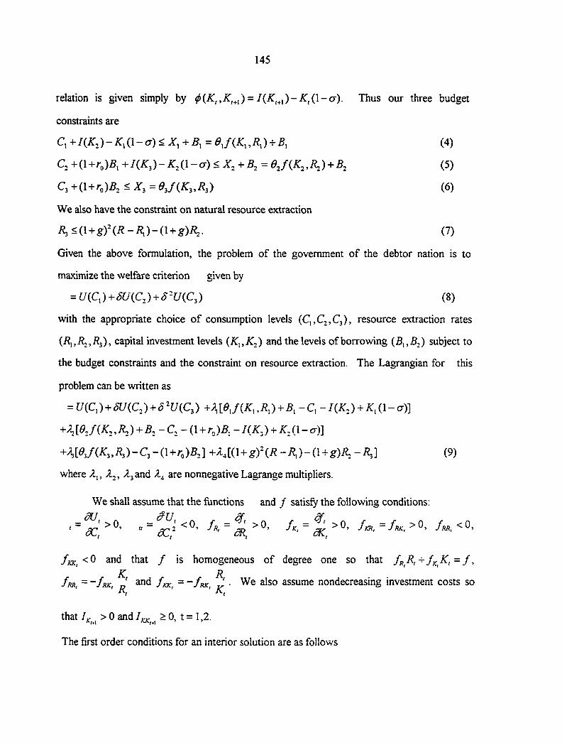
145
relation is given simply by (f>{K,,K,^^) = Thus our three budget
constraints are
Q + ) -K , ( \ -a )<X ,+B,= dJ iK , ,R , ) + B , (4)
C + (1 + )B, + I{K, )-K^{\-a)<X^^B,= ej{K, ,11J + B, (5)
C3 +( l + ro )5 , < 3 = dJ{K„R, ) (6)
We also have the constraint on natural resource extraction
il,<(l + g)^(i?-/2,)-(l + g)i^.. (7)
Given the above formulation, the problem of the government of the debtor nation is to
maximize the welfare criterion given by
= U{C, )+SU{C. ) + 5 -U{C^) (8)
with the appropriate choice of consumption levels (C,,C2,C3), resource extraction rates
capital investment levels and the levels of borrowing subject to
the budget constraints and the constraint on resource extraction. The Lagrangian for this
problem can be vwitten as
= U{C,)^5U{C.)^5-U{C^) +^_ej{K,,R{) + B, -C, -/(/:,)+ /:,(!-cr)]
+;ij [e j {K . , /?,) + - C - (1 + )B, - I (K , ) + /:, (1 - cr)]
+W(/C3,i?3)-C3-(l+ro)5J+A,[(l + g)^(;?-/?,)-(l + g)/^-i23] (9)
where A^and /I4 are nonnegative Lagrange multipliers.
We shall assume that the functions and / satisfy the following conditions:
fKK^ < 0 and that / is homogeneous of degree one so that /r R, +/k = f ,
K R Irr, = ~/kjc, /fj. = -/^ '. We also assume nondecreasing investment costs so
' Rt ' '
that If. >0 and 7™ > 0, t = 1,2.
The first order conditions for an interior solution are as follows
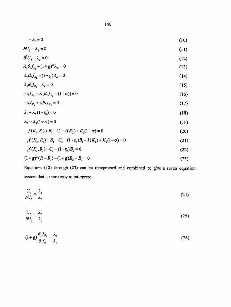
146
, - A , = 0 ( 1 0 )
<51/,-Aj=0 (11)
d-U^-2.^ = 0 (12)
-0+^)'^4=o (13)
^2^24-0 + )^=0 (14)
~^4 (15)
-A^k,+M^2/K,+0-'^)] = ^ (16)
-A^x,+Wk,=0 (17)
A , - A , ( l + r o ) = 0 ( 1 8 )
A,-A3(l+ro) = 0 (19)
,/(/:„/?,)+5,-C,-/(^3) + ,(l-cr) = 0 (20)
J{K.,R.) + 5, - C - (1 +ro)5, - I{K^) + /C,(l - a) = 0 (21)
J{K^,R,)-C,-{\+r^)B^ = {i (22)
(l + )^(i?-i?.)-(l + g)/?,-i^ = 0 (23)
Equations (10) through (23) can be reexpressed and combined to give a seven equation
system that is more easy to interprete.
U, A,
5U. " 2,
U. A,
5U, ~ A,
(26)
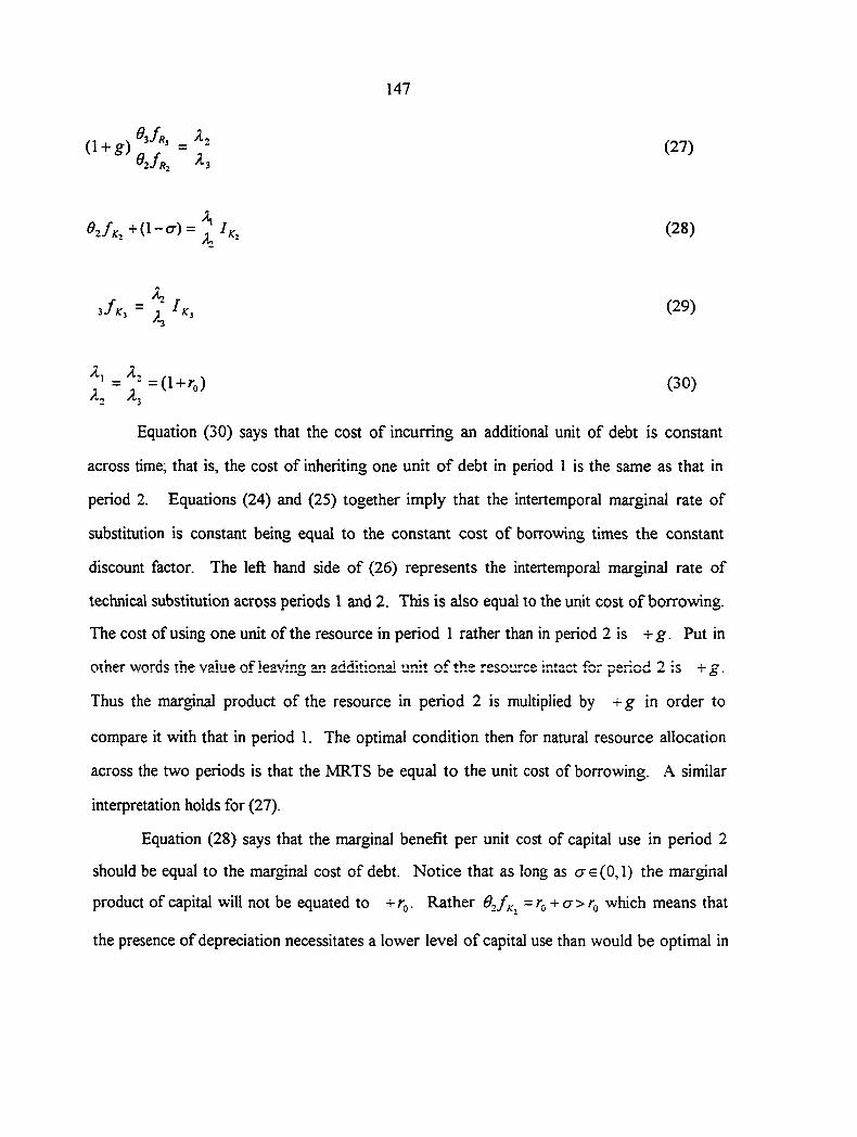
147
(27)
(28)
(29)
(30)
Equation (30) says that the cost of incurring an additional unit of debt is constant
across time; that is, the cost of inheriting one unit of debt in period 1 is the same as that in
period 2. Equations (24) and (25) together imply that the intertemporal marginal rate of
substitution is constant being equal to the constant cost of borrowing times the constant
discount factor. The left hand side of (26) represents the intertemporal marginal rate of
technical substitution across periods 1 and 2. This is also equal to the unit cost of borrowing.
The cost of using one unit of the resource in period 1 rather than in period 2 is +g. Put in
o the r words t he va iue o f l eav ing an add i t i ona ! un i t o f t he r e sou rce in t ac t f o r pe r iod 2 i s + g .
Thus the marginal product of the resource in period 2 is multiplied by +g in order to
compare it with that in period 1. The optimal condition then for natural resource allocation
across the two periods is that the MRTS be equal to the unit cost of borrowing. A similar
interpretation holds for (27).
Equation (28) says that the marginal benefit per unit cost of capital use in period 2
should be equal to the marginal cost of debt. Notice that as long as ere(0,1) the marginal
product of capital will not be equated to +rg. Rather ='b +<^>'0 which means that
the presence of depreciation necessitates a lower level of capital use than would be optimal in
148
the absence of depreciation. Also since 62/k. =^o + ^+^0 the level of capital use will be
higher than that which would pertain in the case of circulating capital (fiill depreciation).
Equation (29) suggests that the marginal product of capital in period 3 per unit investment
cost is equal to the unit cost of borrowing at the optimum.
Substituting (30) into (26) through (29) and using (23) we have five independent
equations in five endogenous variables i?,, R,, R^, and which means that we can solve
for these variables uniquely from the five equation set in terms of the exogenous parameters.
In particular, the optimal input use levels are not functions of S, the discount factor. This
suggests a separation of production choices from consumption decisions. The reason for this
is the presence of borrowing oppotunities in the international capital market.
We will now proceed to analyze comparative static effects of the exogenous
parameters on the levels of the choice variables.
4.1: Comparative Statics In No-Default Deterministic Model
In order to obtain comparative static results for all the parameters we first totally
differentiate the system of first order conditions. Then we ran a Maple V Release 2 program
which produced comparative static expressions not presented here. The expressions are
available upon request from the author. The signs of these comparative static derivatives are
summarized in Table 1.
Table 1 shows that an increase in the discount factor leads to a deferrment in
consumption and a decline in the level of borrowing. However, it has no impact on input
allocations in the model with no default risk. An increase in the growth rate of the natural
resource acts as an income effect that leads to increased consumption in all periods; but it also
leads to a deferrment in resource extraction and capital investment while its impact on the
levels of borrowing is ambiguous. An increase in the initial capital stock has an income effect.
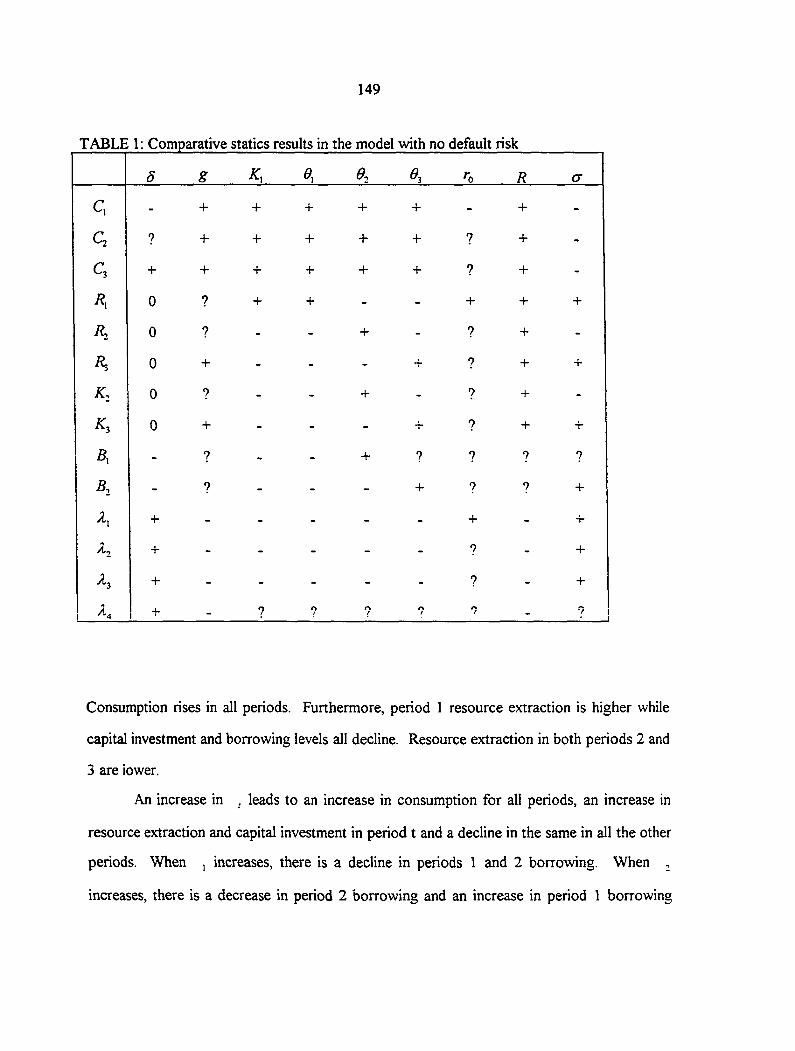
149
TABLE 1: Comparative statics results in the model with no default risk
C
•^2
A
/I,
9
+
0
0
0
0
0
+
+
+
+
+
+
?
?
+
?
+
?
9
A +
+
A. + +
+
+
A. +
+
+
+
+
A +
+
+
+
+
?
+
?
?
+
?
?
?
?
?
?
+
?
9
+
+
+
+
+
+
?
9
+
+
?
+
+
-4 I
Consumption rises in all periods. Furthermore, period 1 resource extraction is higher while
capital investment and borrowing levels all decline. Resource extraction in both periods 2 and
3 are lower.
An increase in , leads to an increase in consumption for all periods, an increase in
resource extraction and capital investment in period t and a decline in the same in all the other
periods. When , increases, there is a decline in periods 1 and 2 borrowing. When ,
increases, there is a decrease in period 2 borrowing and an increase in period 1 borrowing

150
while for an increase in 3 there is a decline in period 2 borrowing, but the impact on period 1
borrowing is ambiguous.
For an increase in the world rate of interest, period 1 consumption falls and resource
extraction in the same period rises. All other effects are contingent on the realizations of
other parameters. A higher initial resource stock has a pure income effect, leading to an
increase in consumption, resource extraction and capital stock in all periods. Its impact on
borrowing is, however, ambiguous. Finally a higher rate of depreciation means lower
consumption in all periods and a decline in period 2 investment and resource extraction while
for the other periods the input levels rise. It also means a higher level of period 2 borrowing,
leaving an ambiguous impact on period 1 borrowing.
151
5: MODEL WITH DEFAULT POSSIBILITY AND INCOWIE UNCERTAINTY
In this section we introduce the possibility that the debtor nation will default on its
debt payment obligations. As in the earlier section borrowing is allowed in periods 1 and 2.
Payment is required in period 2 for period 1 borrowing and in period 3 for period 2
borrowing. In this section the realization of the period 2 income shock, is not known at
the beginning of the initial period. However, 6^ is known for certain at the very beginning, as
well as the period 1 shock, 0^. Thus both lenders and debtors form expectations about ft.
We assume that the subjective distribution of 0 is the same for creditors and debtors and that
the mean E[6\= $ and variance var(^ = Vg are common knowledge at the beginning of the
initial period.
Debtors will make their default decisions based on optimality criteria. Thus default
occurs if the expected utility from the default decision exceeds that from the no-default
decision. Default risk arises from the uncertainty introduced by 0, because future realizations
of 0 may differ from expectations, making it necessary for the debtor nation to revise its
decisions. As we mentioned above, the probability density function of , is common
knowledge fironi the beginning of the planning horizon. The penalty for default is an
exemption from flirther borrowing and also from international trade in general. Though not
modeled explicitly here, we suppose that the exemption from trade causes a reduction in
debtor nation income. Again we can imagine this to be explained by the possibility that
exclusion from trade means that it is now difficult for the debtor nation to purchase some
inputs required for its production process. This we assume, leads to a reduction in
productivity. Alternatively this can be explained by the possibility that the debtor nation is
excluded from trading with most nations and now has to purchase needed inputs at higher
than usual prices from some other country. Thus the reduction in income could in this case be
152
represented by a fall in the debtor nation's terms of trade. Either one or both of the above
motivations could be implied in this model. We introduce this income reduction
multiplicatively by a parameter y €(0,1). The lower is y, the stronger is the impact of the
trade exemption on the debtor nation. We assume that y is common knowledge at the
beginning of the plarming horizon. The default penalty is imposed in the period of default and
the debtor loses credit worthiness so that the penalty is maintained for all succeeding periods.
5.1: Creditor Response To Default Risk
In view of the default risk and the fact that creditors receive no remuneration when
this occurs we suppose that they adjust the lending terms to prevent or minimize any losses
from the occurrence of a defauh. Let tt be the creditors' subjective probability that the debtor
vwll default. We assume that the higher the level of borrowing, B, the more it costs the
debtor to repay and thus the more likely a default. Thus, though yet to be proven, k is
modeled here as decreasing in B. Later, this can be shown to be consistent with the
optimization behavior of economic agents. We also expect to be a function of 9 and v^,
the mean and variance of the distribution of Q. We assume that tz as a function of B is
knowTi to debtor nation as well.
The creditor eams for each unit of capital invested in its domestic economy at
the risk-free rate of interest r^. If it lends this capital to a debtor nation at a rate r>ro, its
returns, PR are
0 with probability -7t
Thus in a perfectly competitive setting the creditors' loan supply schedule is obtained by
solving
l + r with probability 71
153
^'B;0,v^)(l+r) = (l+ro) (32)
whence we obtain
r = (33)
As /r is decreasing'm B, r will be increasing in 5. As a final qualification, we expect that
there is a level of borrowing, B beyond which the probability of no-default is zero. That is
\7t{B\e ,Vg) for B<B
^~l 0 for B>B ^
Thus the resulting loan supply schedule is more specifically
\r(B;e ,Vg,r^) for B<B
'n « forB>B
In other words a credit ceiling is imposed. We will now proceed to outline the nature of the
problem with default risk and its impact on resource allocation.
Let us assume the optimization framework in section 4 with the following
modifications. There is a positive probability of default. Default in period 2 leads to a ban
from fiirther borrowing in period 2 and from trade in periods 2 and 3. A default in period 3
leads to a ban fi-om trade in period 3. The interest rate on borrowangs made in period t is
r, =r(Bj;0,Vg,rQ), t = 1,2. We shall also assume that the realization of 3 is knowm in
advance and is equal to . Thus default risk is prompted by uncertainty in period 2 income.
At the beginning of each period 1, , is realized so that only is unknown at the beginning
of the planning horizon.
154
The decision problem confronting the debtor nation and the various outcomes in this
model can be illustrated by the game tree in Figure 5.1 . The decision nodes are numbered to
correspond to periods. Default/No-Default decisions are potentially made at nodes 2 and 3.
Once a default decision is made no further decisions are needed since the choice variables for
the rest of the planning horizon are determined.
In period 1 the debtor nation starts off with a capital stock AT, and resource stock R
and 9^ is known. Based upon this information set the debtor nation chooses the levels of the
period 1 variables and makes contingent plans for the period 2 and 3 variables in order to
maximize utility over the three period planning horizon. The levels of the period 1 decision
variables are functions of the technology parameters, of and the expectations about
that is, its mean and and variance g'. Let the probability density function of 6^, which is
common knowledge, be represented by ). Then the expected value of 0., is given as
= £(9^)=
Also £(&•,') = J 6^ p{0^)d6^ and the variance of is
2 J7r 2 T / r^r /o -IN 2
Upon the arrival of period 2, the uncertainty about is resolved and the debtor nation
revises its optimal solution for periods 2 and 3 decision variables. Let us first suppose that it
pays off its debt. It may thus borrow again and decide in period 3 whether to default or not.
However, since there is no uncertainty in period 3 one would expect that the creditor would
respond by adjusting the lending terms so that it is never optimal to default in period 3. It is
easier to approach this problem through a backward induction approach. Thus suppose we
are in period 3. ATj is known, being determined by the period 2 investment decision. is
knov^ since by the resource constraint, R^ = {\-\- g)- {R - R^) - {\ + g)R,. In the absence of
income uncertainty it means that the only period 3 decision is the allocation of income

155
3 P
Defaulj
1 Borrow
Default Not Default and borrow more
No^ Default
Figure 5.1 Decision Tree of Debtor Nation
between consumption and debt payment. If the debtor nation decides to make full payment
its period 3 consimiption will be = 5/(/Cj, ) - (1 + /-j) . (36)
If ii decides to default, period 3 consumption would be
(37)
Thus it will default if and only if
(38)
Thus to prevent default in period 3 the bank will impose the credit ceiling
= (39)
156
Since this credit ceiling eliminates the possibility for period 3 defauh given that the
debtor nation acts optimally, the probability of no-default in period 3 is 1. Thus the interest
rate charged on 5, will be r^. That is, rj = so that
Thus for any given production isoquant the credit ceiling for the debtor is known. We
suppose that for this to be feasible the level of borrowing in period 2 is conditional on the
levels of ATj and so that K^, R, and 5, are chosen simultaneously.
Given the credit ceiling and that C, is given as a function of 5, we move to the next phase of
optimization. The debtor nation chooses C, /?,, and 5, to maximize utility for the
remaining horizon. More formally it solves;
(l + rj (40)
Max
C2 , »-^2 ' 3 subject to
UiC.J + SUiC,) (41)
(1 + r,)B, + C, + I(K,) - a:, (1 -0-) < ejiK.,R.) + 5, and
C, = enK„R,)-{l+r,)B,
The Lagrangian for this problem is
i , ' =U(C,) + SU(efiK„R,)-i \ + r,)B,)
The first order conditions will then be
, - A , = 0 (42)
157
(43)
(44)
(l + 'o)^3 ^ J{K^,/?,)- (1 + r, )5, + 5, - C, - /(/Cj) + /:, (1 - cr) = 0
(45)
(46)
l+'b''
Let us first consider an interior solution for C,, and R^. Firstly (42) and (45) imply that
When the debt constraint is binding, <j)>0. When it is not binding, ^ = 0. When the debt
constraint is binding the intertemporal marginal rate of substitution (MRS) is +ro. Thus
when the debt constraint is binding, the intertemporal marginal rate of substitution is higher
than when it is not binding.
The marginal products of the capital and natural resource inputs are also affected by
the debt constraint. We have from (44) and (45) that
However, the intratemporal marginal rates of technical substitution are not affected by
whether the constraint is binding or not. We have in both cases.
71 =1 =—— ;—>1 + u, su,
Similarly,
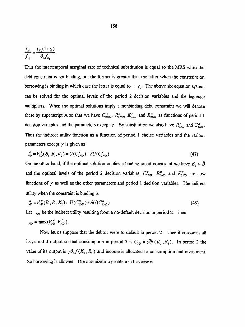
158
Ik, _ 4.(l + g)
/rj
Thus the intertemporal marginal rate of technical substitution is equal to the MRS when the
debt constraint is not binding, but the former is greater than the latter when the constraint on
borrowing is binding in which case the latter is equal to + Tq. The above six equation system
can be solved for the optimal levels of the period 2 decision variables and the lagrange
multipliers. When the optimal solutions imply a nonbinding debt constraint we will denote
these by superscript A so that we have ^nd' functions of period 1
decision variables and the parameters except y. By substitution we also have and .
Thus the indirect utility function as a function of period 1 choice variables and the various
parameters except y is given as
On the other hand, if the optimal solution implies a binding credit constraint we have B.^= B
and the optimal levels of the period 2 decision variables, and are now
functions of y as well as the other parameters and period 1 decision variables. The indirect
Let ^ be the indirect utility resulting firom a no-default decision in period 2. Then
Now let us suppose that the debtor were to default in period 2. Then it consumes all
its period 3 output so that consumption in period 3 is {K^,R^). In period 2 the
value of its output is y9^f{K^,R,) and income is allocated to consumption and investment.
No borrowing is allowed. The optimization problem in this case is
^=V^{B„R„K,) = Uia^)+6U{C^^) (47)
utility when the constraint is binding is
(48)
^ = m a x ( F ^ , F ^ ) .
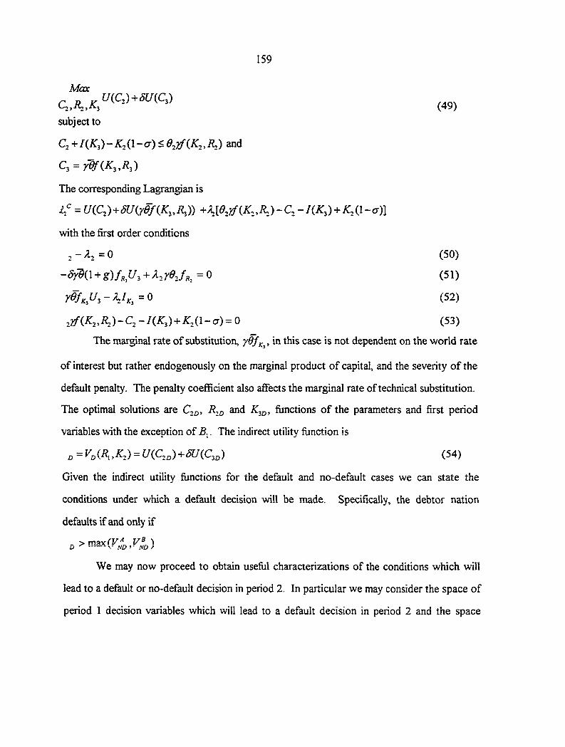
159
Max UiC,)+SU(C,)
2 > ' 3 (49)
subject to
C,+I(K,)-K,{l-a)<0,j f iK,, l l)and
C, = rWiK„R,)
The corresponding Lagrangian is
If =U(C,)+dUirefiK,,R,)) +A,[e._TfiK„R,)-a-IiK,) + K,il-cx)]
with the first order conditions
2 ~ ^2 ~ ^
- Sydo+g)fRU^+A, re.jr, = o =0
, j f (K„R,)-C,-l(K,) + K,i l-a) = 0
(50)
(51)
(52)
(53)
The marginal rate of substitution, ydf^^, in this case is not dependent on the world rate
of interest but rather endogenously on the marginal product of capital, and the severity of the
default penalty. The penalty coefficient also affects the marginal rate of technical substitution.
The optimal solutions are R^d and functions of the parameters and first period
variables with the exception of 5.. The indirect utility function is
Given the indirect utility functions for the default and no-default cases we can state the
conditions under which a default decision will be made. Specifically, the debtor nation
defaults if and only if
. > n i f l v r F l v ^ \ u v hd ' • so >
We may now proceed to obtain useful characterizations of the conditions which will
lead to a default or no-default decision in period 2. In particular we may consider the space of
period 1 decision variables which will lead to a default decision in period 2 and the space
^ =Fo(/?„^,) = f/(CJ+<5C/(C3o) (54)
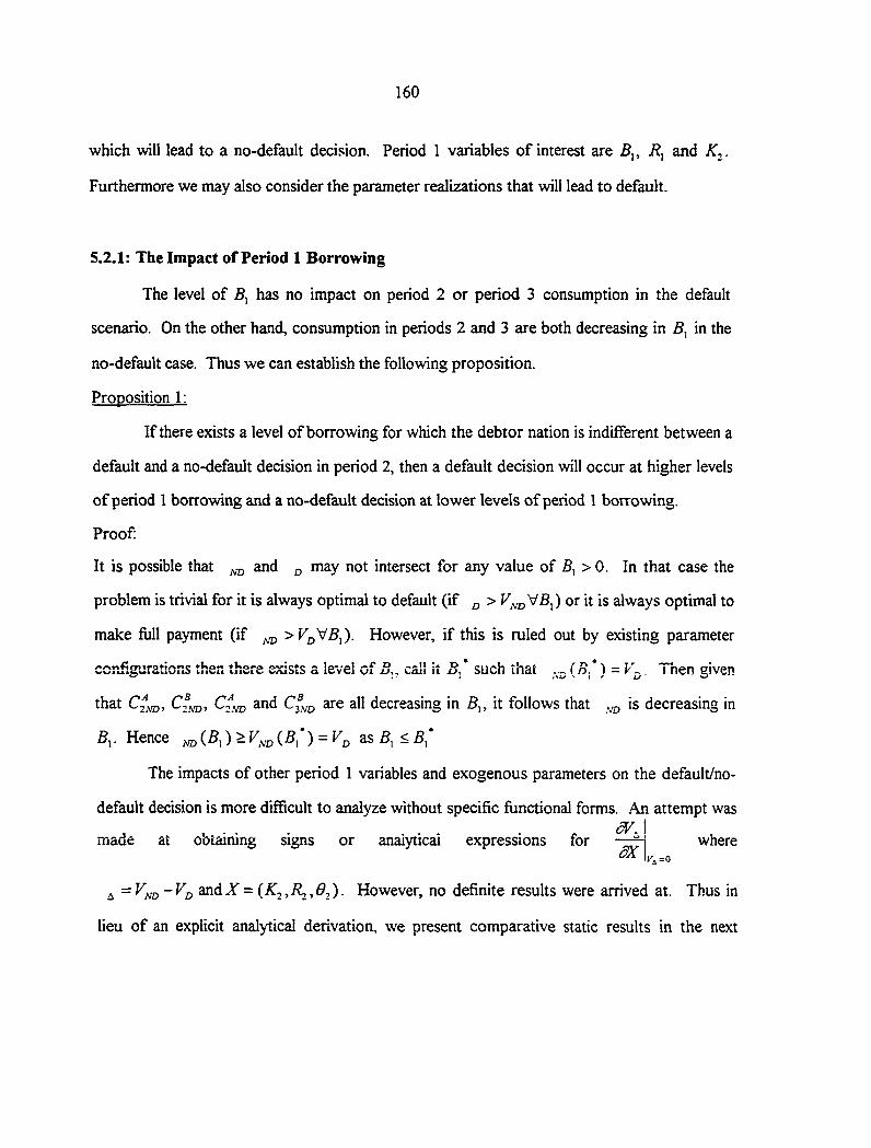
160
which will lead to a no-default decision. Period 1 variables of interest are 5,, i?, and K^.
Furthermore we may also consider the parameter realizations that will lead to default.
5.2.1: The Impact of Period 1 Borrowing
The level of 5, has no impact on period 2 or period 3 consumption in the default
scenario. On the other hand, consumption in periods 2 and 3 are both decreasing in in the
no-default case. Thus we can establish the following proposition.
Proposition 1:
If there exists a level of borrowing for which the debtor nation is indifferent between a
default and a no-default decision in period 2, then a default decision will occur at higher levels
of period I borrowing and a no-default decision at lower levels of period 1 borrowing.
Proof
It is possible that ^ and ^ may not intersect for any value of 5, > 0. In that case the
problem is trivial for it is always optimal to default (if ^ ) or it is always optimal to
make full payment (if ^ >V,^\/BJ. However, if this is ruled out by existing parameter
configurations then there exists a level of B,, call it B, ' such that (o,* ) = V^. Then given
that Qm)' ^2nd decreasing in 5,, it follows that is decreasing in
5,. Hence ^(5,) >^^(5,*) = as <5,*
The impacts of other period 1 variables and exogenous parameters on the default/no-
default decision is more difficult to analyze without specific functional forms. An attempt was
made at obtaining signs or analytical expressions for ^ where
^ andX = However, no definite results were arrived at. Thus in
lieu of an explicit analytical derivation, we present comparative static results in the next
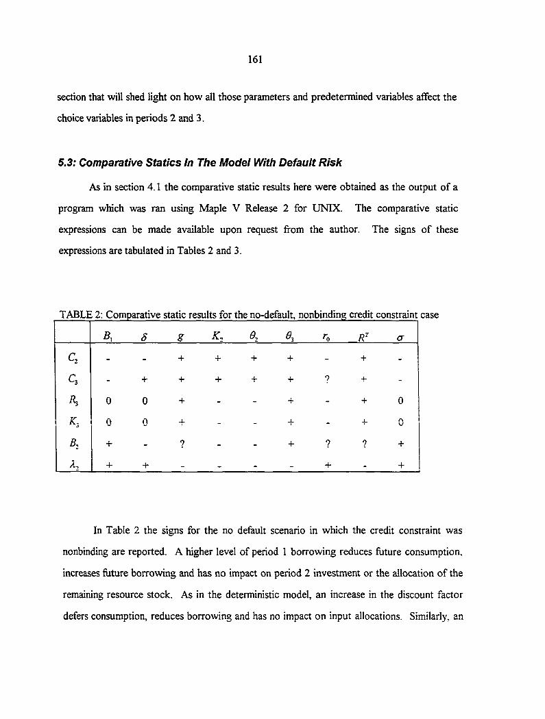
161
section that will shed light on how all those parameters and predetermined variables aifect the
choice variables in periods 2 and 3.
5.3; Comparative Statics in The IVIodei With Default Rislt
As in section 4.1 the comparative static resuhs here were obtained as the output of a
program which was ran using Maple V Release 2 for UNIX. The comparative static
expressions can be made available upon request from the author. The signs of these
expressions are tabulated in Tables 2 and 3.
TABLE 2: Comparative static results for the no-default, nonbinding credit constraint case
s g K. 9. 9 , cr
- - + + + + - + -
Q - + + + + + 9 + -
0 0 + + - + 0
0 0 4- -U -
j- yj
B2 + - ? + ? ? +
A, + + - - + - +
In Table 2 the signs for the no default scenario in which the credit constraint was
nonbinding are reported. A higher level of period 1 borrowing reduces future consumption,
increases future borrowing and has no impact on period 2 investment or the allocation of the
remaining resource stock. As in the deterministic model, an increase in the discount factor
defers consumption, reduces borrowing and has no impact on input allocations. Similarly, an
162
increase in the growth rate of the natural resource leads to an increase in period 3 resource
extraction and capital stock and an increase in consumption for all periods while the impact on
borrowing is ambiguous.
A higher period 1 investment (period 2 capital stock) means more consumption in
periods 2 and 3 but less borrowing in period 2 and less resource extraction and capital stock in
periods. The same holds for an increase in An increase in 3 on the other hand leads to
an increase in periods 2 and 3 consumption, period 2 borrowing, and period 3 input levels.
Once again, a higher interest rate leads to deferred consumption. It also means decreased
period 3 resource extraction and capital stock but an ambiguous impact on borrowing. An
increase in the remaining stock of resources again has an income effect while an increase in
the rate of depreciation reduces consumption in both periods and increases borrowing in
period2. However, unlike the deterministic case it has no impact on period 3 resource
extraction or capital stock.
Comparing Tables 2 and 3 we notice some significant differences. In the default case
represented in Table 3 a higher discount factor defers consumption as in the no default case,
but this time it leads also to an increase in period 3 resource extraction and capital stock. A
higher growth rate of the resource promotes deferrment of extraction to period 3 but a decline
in period 2 investment for period 3 and also a decline in period 2 consumption. A higher 3 is
more of a substitution effect this time as consumption in period 3 rises at the expense of that
in period 2. Finally, an increase in the rate of depreciation leads to lower levels of resource
extraction and capital stock in period 3 unlike the deterministic case where the impact was
positive and the no default case in Table 2 where there was no impact.
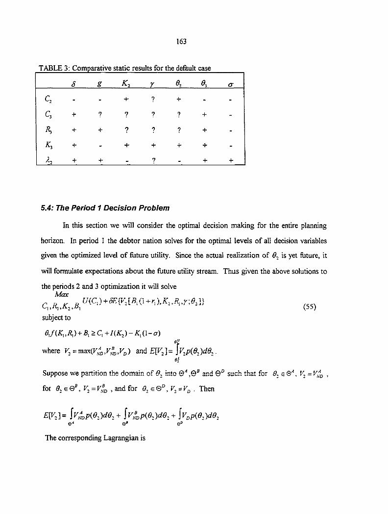
163
TABLE 3: Comparative static results for the default case
g A:. 0. ^3 cr
a - + ? + - -
C3 + ? 7 ? ? + -
^ + + 7 7 7 + -
K, -f - + + + + -
+ + - ? - + +
5.4: The Period 1 Decision Problem
In this section we wall consider the optimal decision making for the entire planning
horizon. In period 1 the debtor nation solves for the optimal levels of all decision variables
given the optimized level of future utility. Since the actual realization of is yet future, it
will formulate expectations about the future utility stream. Thus given the above solutions to
the periods 2 and 3 optimization it will solve Max
(55)
subject to
+ > C, +I{K^) - K,{\-a) qV
where F, = max(F4E\y^] = JV,p{e.^)dG,. ^2
Suppose we partition the domain of into 0'^ ,0^ and 0° such that for s , V., = ,
for ^,€0®, V^ = V^ ,and for = . Then
6'' e' e"
The corresponding Lagrangian is
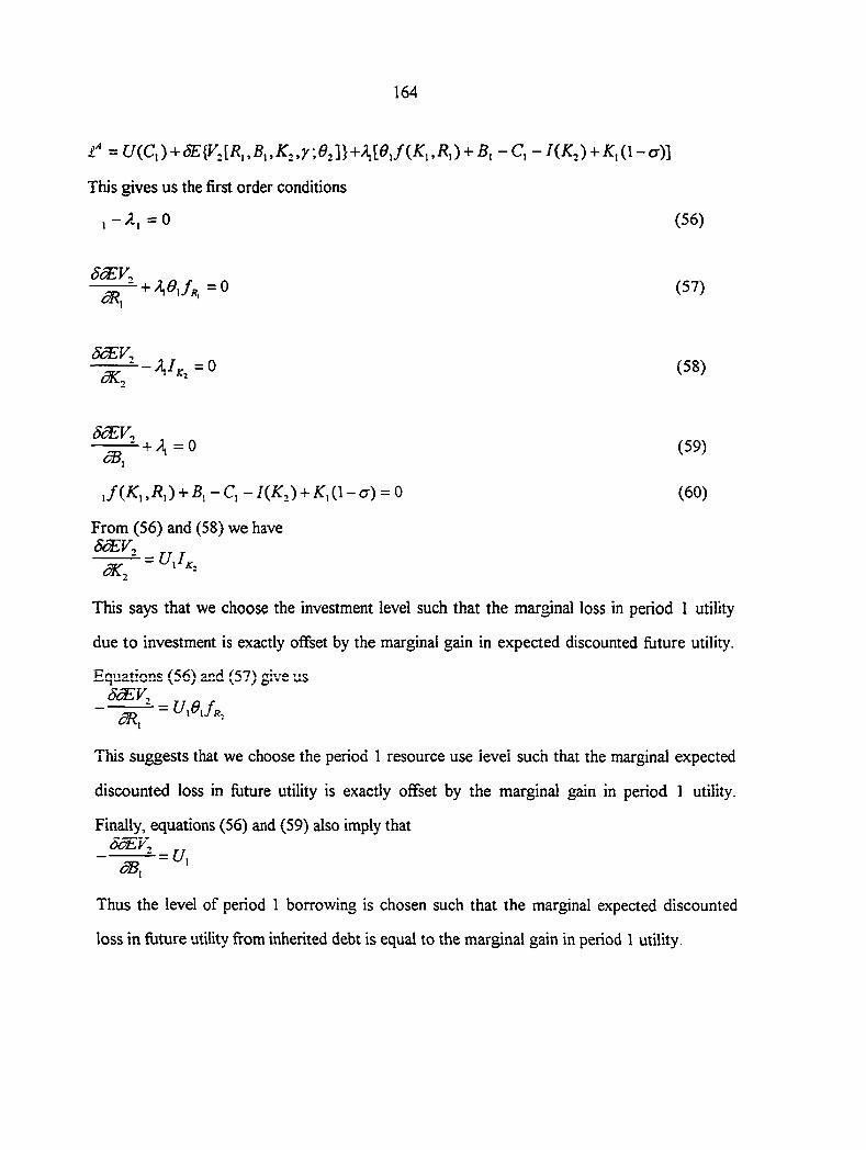
164
t U{C,) + SE{V,[R„B„K„r,e,]}+^[OJiK„R,) + B,-C,-I{K,) + K,{\-cr)]
This gives us the first order conditions
,-A, =0 (56)
-^ + W«. =0 (57)
^ - V . . = 0 ( 5 8 )
+ / ^ , = 0 ( 5 9 ) cB,
JiK, ,R,) + B,-C,-l{K,) + K,i\-(7) = 0 (60)
From (56) and (58) we have
^ = c / / ac '
This says that we choose the investment level such that the marginal loss in period 1 utility
due to investment is exactly offset by the marginal gain in expected discounted future utility.
Pnu5»tir>nc ^ o r t A ( ^ ' 1 \ dcEV
—: = UAfR I \JR.
This suggests that we choose the period 1 resource use level such that the marginal expected
discounted loss in future utility is exactly offset by the marginal gain in period 1 utility.
Finally, equations (56) and (59) also imply that d^y\
<2ZJ,
Thus the level of period 1 borrowing is chosen such that the marginal expected discounted
loss in future utility fi:om inherited debt is equal to the marginal gain in period 1 utility.
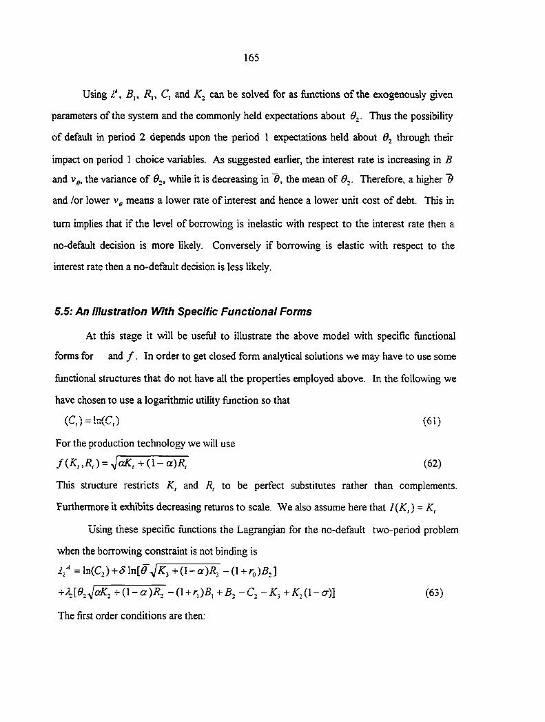
165
Using I*, 5,, i?,, C, and can be solved for as functions of the exogenously given
parameters of the system and the commonly held expectations about dj. Thus the possibility
of default in period 2 depends upon the period 1 expectations held about through their
impact on period 1 choice variables. As suggested earlier, the interest rate is increasing in B
and Vg, the variance of $2, while it is decreasing in 9, the mean of 0,. Therefore, a higher 9
and /or lower means a lower rate of interest and hence a lower unit cost of debt. This in
turn implies that if the level of borrowing is inelastic with respect to the interest rate then a
no-default decision is more likely. Conversely if borrowing is elastic with respect to the
interest rate then a no-default decision is less likely.
5.5: An Illustration With Specific Functional Forms
At this stage it will be useful to illustrate the above model with specific functional
forms for and /. In order to get closed form analytical solutions we may have to use some
functional structures that do not have all the properties employed above. In the following we
have chosen to use a logarithmic utility function so that
fr \ - \ .nrr \ f — f VDl^ t
For the production technology we will use
f iK, ,R,) = (xK, +{ \ -a)R, (62)
This structure restricts K, and R, to be perfect substitutes rather than complements.
Fur thermore i t exhib i t s decreas ing re turns to sca le . We also assume here tha t 1{K,) = K,
Using these specific functions the Lagrangian for the no-default two-period problem
when the borrowing constraint is not binding is
i ," =ln(C^) + S\n[e^K,+(\ -a)R, - ( \ + r, )B,]
- (1 + )B, + 5, -C2-K,+ K,(1 - a)] (63)
The first order conditions are then;
166
-mi + gXl-a) . ^g , ( l -a)
Iz^yjoK^ +(1- a) i?3 l^ccK^ +( l -a)R,
SBa
2z^aK^ +(1- a)/?3 = 0
-^(l + O , A, =0
,y lccK,+i l -a)R.-( \ + r, )B, +B,-C.-K^+K.i \ -<T)
where = 0 ccK^ +(l-a)/?3 - (1 + Tq )5,
Solving (65), (66) and (67) we get (69) and (70)
r ^.3 T
r ae 1
From (69) we solve for Ry as
{ae,f-Aa{\ + gfK, 4(l-a)(l + g)^
Applying the natural resource constraint to (71) we get
167
A{\ + gf{( \-a)R'^aK,]-{ae,y
' 4(l-a)( l + )
Then substituting from (72) into (70) we obtain K,
aef . (af t ) ' -4(H-g) ' t ( l -g)«"tgg,]
"® [2(l+r„)]= 4(l-a)(i+g) < '
At this stage 5, and C, can be solved for simultaneously from (64) and (68)
ae\2+5) S \ _ aO,- (1+?) ^ 1
C* =• ^2A/D 1 aO
2 +^2(1 —cr) + (1+g) ,
2(I + )-(1+''.)^.+^-^[0-«)^'+^2]|(75) (1 + ) [4( l+ro)
Since C3 is equal to period 3 output minus debt payments in that period we have
<5(l+ro)f ae ad^ (1 + ),
Thus the indircct utility functiGn for the no~dcikult cesc when tnc constraint on 5-, is not
binding is given as
I-hS)
[^(l+rf (77)
When the constraint on period 2 borrowing is binding we can proceed in a similar
fashion. The Lagrangian is now
= ln(C2 +C) + d\n[yd yJocK^ +{l-a)R^ ] (78)
168
+\{e. aK^+i\-a)R. - (1+r, )B, + ^ \e 4aK,+{\-a)R^ - Q - (1 - a)]
The first order conditions are;
^ -^=0 (79)
-Sm+gXl-a) , A,^(l + g)(l-a) j l-y) ,
2r,ylaK,+(\-a)R^ +(1-a)R^ 2^aK^+ i^-a)R^ (l + r j
——M^=-a 0-y ) . .gj.
2r,Va^3+(l-a)i?3 ' l^aK,+{\-a)R, (l + r^)
0 ,yjaK^+(l-a)R,-( l+r,)B,+^-^e^aK,+(\-a)R, -C.-K,+K.i \-a) = 0 (82)
where T^=yO -^jocK^ + (1 - a )R^
The solutions yield the same R, and R^ levels as before.
{ad^f -Aa{\ + g)-K, '^2ND ~ , v s 2 4 i j -Qr)(! + g;
•^2M3 ~ •
4(1 + g)- [(1 - a)R' + - (a^, )^-3nd - 77; tt; ;
4(l-o:)(i + g)
After various manipulations we obtain the optimal levels of consumption and period 2 capital
investment as follows
^2ND ~ {^^0 + 2fo-y/^o' "*"^1 "*"^1 I (83)
= 7 " + ^ 2 ^ 0 V v + f , + + ^ o " + ^ 0 jso'+s, + a;:, + (1 - a);?''](84) 8a 8a ' 2 4(1+^) a
169
yd ^3ND ~ ^ I 2^0 V^O ^1 I (85)
where jj. = g(l + g)(l-;^)
(l + /-o) '
ad^ 4 (2+<?) 2
(1 + g)"^ 5a a
rf2a-(l + g)l (2^
8a(l + ^) ' 4Ja
The indirect utility function in this case is
B nd "*"^1 "*"^1 i" I ^ + £j +£] (86)
The defauh scenario can also be solved using the same functional structures defined
above. The Lagrangian for the two-period optimization is given as
Lf =\n{C.^+6\viyd4cd<:^+(\-a)R,]+^ye.JaK.+{\-a)R, -C,-ATj+/:,(!-a)] (87)
The first order conditions for an interior solution are;
c ^ (88)
-Sr&(l + g) i \ - a ) ^ A , y d , ( \ - a )
2 r , yjoK^ +(1- a) i?3 +(1 - a)i? . (89)
Sf&a
2z- , +(1- a) /?3 2 , = 0 (90)

170
+(1-«)-^ -Q -K^+Kj{\-o) - 0 (91)
where , = 'JocK^+(l-a)Ri as before
In this case the optimal natural resource extraction rates are
4(l-a)(l + )^
„ 4i \ + g) ' [ i l -a)R' +aK,]-{raO,y-4(l-«)(l + g)
Comparing the resource extraction rates under this default scenario with that pertaining in the
case of the no-default scenario produces some useful results. We note that
n _ . A + >»• (94)
Thus we can draw the following conclusion.
Proposition 2:
Given our production structure and logarithmic utility function the default scenario delays the
extraction of resources relative to the no-default scenario.
The capital investment in period 2 for the default scenario turns out to b£
air02y-i l+S)-4{l + g) \ l -a)R'+2i \ + g)K,[S(\ -cT)-2( \ + g)] 2{ \ + g )i2 + S )

171
By similar manipulations we can get the consumption levels for both periods as functions of
the exogenous parameters of the system.
(96)
5a
T (97)
The indirect utility function for the default scenario is thus given by
,=wo^y 5a
V 2
a(Af , 2(HgXl-«)^
L2(l+g) (2+5) +A^[{2(l+g>5-lKl-o)+4(l+g)=] (98)
5.6; Simulations For The Period 2 Decision Problem
In this section we present results of computer simulations comparing the indirect utility
functions for the three scenarios analyzed: default, no-default with binding credit constraint at
the optimum, and no-default with nonbinding credit constraint at the optimum. In these
simulations the period 1 decision variables have not been solved for but are rather taken as
given. Thus we plot the various indirect utility functions against 5,, K^, /?,, and for
various parameter scenarios. These plots are presented in Figures 5.2 and 5.3. We used the
specific functional forms defined in Section 5.4 for all these simulations. For all the computer
172
simulations we used the Maple V software package for UNIX. No simulations have been
reported here for the entire planning horizon.
Generally, the indirect utilities for all three scenarios are increasing in 9^, as expected.
It is not clear in general that the no-default utility rises faster with than the default utility.
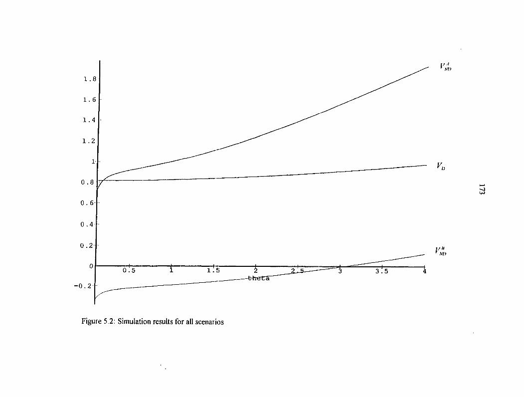
- 0 . 2
Figure 5.2: Simulation results for all scenarios
fn
V" Nl)
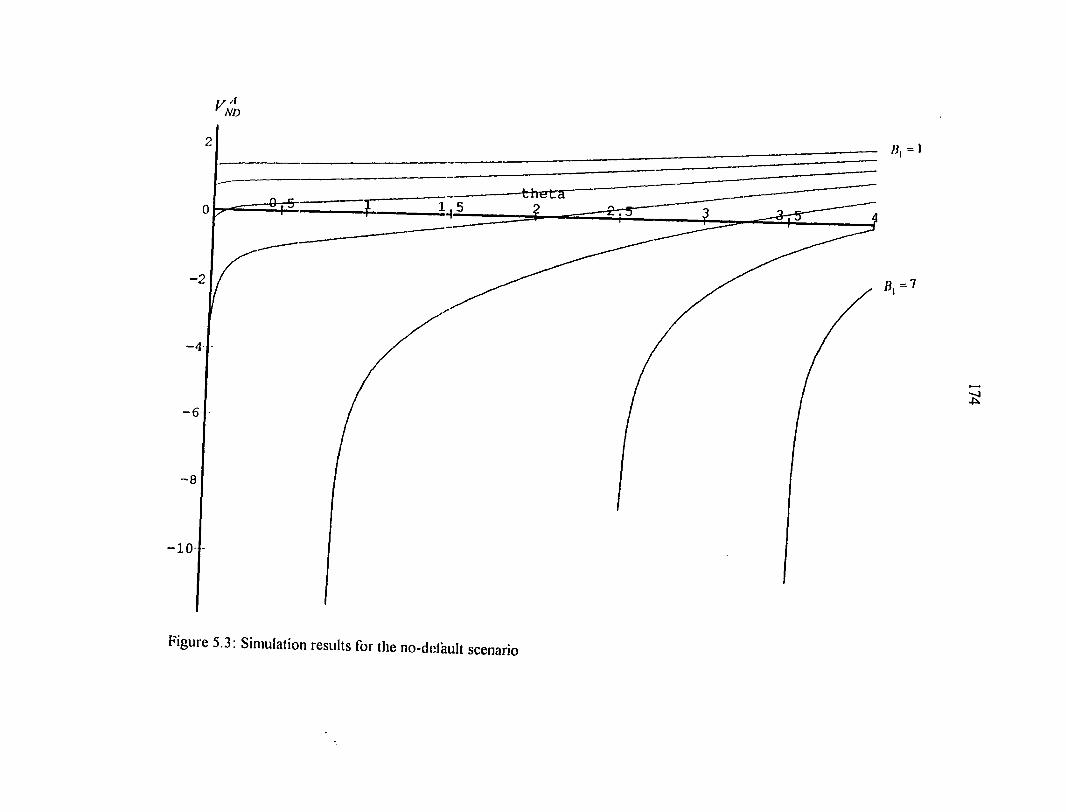
Figure 5.3: Simulation results for the no-deiault scenario
/i, = l
175
6: CONCLUSION
Most developing countries rely heavily on their natural resource base as a major source of
income. Natural resources being related to production in the agricultural sector in most cases, this
explmns why for many such countries agriculture accounts for a far greater share of income than
the nonagricultural sectors. In this paper we considered the implications of resource extraction in
such economies when foreign debt is used to finance capital investment. We considered the
possibility of default risk and a likely creditor response.
The results of this paper show that the ability to borrow in an international capital market at
an exogenous interest rate shields resource extraction decisions from the discount rate or the rate
of time preference of the debtor nation. However, when the interest rate is endogenous, being a
function of the level borrowed, the rate of resource extraction is a function of the discount rate, and
as in standard natural resource models, the higher the discount factor, the faster the rate of
extraction. In general a higher interest rate also leads to a faster rate of extraction so that an
increase in either or both of these parameters lead to less conservation of resources.
The debt repayment requirements of a debtor nation imposes a burden on it to rapidly
extract its natural resource reserves in order to meet its obligations. Thus if default were possible,
the default outcome would likely lead to more conservation of the resource than a no default
outcome gjven the same predefault conditions as a country which chooses to repay its debt. The
creditor response was assumed to take into account the variability and mean of debtor nation
income. These resuhs suggest that developing debtor nations might extract their resources more
rapidly if under obligation to pay their debt within a specified period. If debt forgiveness is allowed

176
and expected this might lead to more conservation of the resource, though not explicitly modeled
here.
177
REFERENCES AIZENMAN, Joshua and Eduardo R. Borensztein, "Debt and conditionality under endogenous terms of trade adjustment" in Analytical Issues in Debt, (eds. Frenkel, Dooley, Wickham) IMF, 1989.
AIZENMANN, Joshua, "Investment, Openness, and Country Risk", in Analytical Issues in Debt, (eds. Frenkel, Dooley, Wickham) IMF, 1989.
ALLEN, Franklin "Credit rationing and payment incentives". The Review of Economic Studies, Vol. 50 (October 1983): 639-46.
BACHA, Edmar L., "External debt, net transfers, and growth in developing countries". World Development, Vol. 20, No. 8 (1992): 1183-1192.
BULOW, Jeremy and Kenneth RogoflF, "Sovereign Debt Repurchases: No Cure for Overhang", Quarterly Journal of Economics 106 (Nov. 1991): 1219-1235.
CALVO, Guillermo, "On the time consistency of optimal policy in a monetary economy", E^onometrica, Vol. 46 No. 6 (Nov. 1978): 1411-1428.
CAMPBELL, Tim S. and Yuk-Shee Chan, "Optimal Financial Contracting With Ex Post and Ex Ante Observability Problems", Quarterly Journal of Economics, 107 (May 1992):785-795.
CLINE, William, "International debt and the stability of the world economy", Washington, D.C.: Institute for International Economics, 1983.
COHEN, Daniel, "A valuation formula for LDC debt", Journal of International Economics, 34 (1993): 167-180.
COOPER, Richard N. and Jeffery D. Sachs, "Borrowing Ahead: The Debtor's Perspective", in International Debt and the Developing Countries, (eds. Gordon W. Smith and John T. Cuddington), World Bank Symposium, 1985.
FARDMANESH, Mohsen, "Terms of trade shocks and structural adjustment in a small open economy: Dutch Disease and oil price increases". Journal of Development Economics, 24 (1991): 339-353.
FRIEDMAN, Milton, "The optimum quantity of money and other essay \ Chicaeo: Aldine Publishing Co., 1969.
FRIEDMAN, Milton, "A monetary and fiscal framework for economic stabilization", American Economic Review, 38 (June 1948): 245-264.
178
HELPMAN, Elhanan, "The Simple Analytics of Debt-Equity Swaps", American Economic Review, Vol.79 No.3 (June 1989):440-451.
International Financial Statistics Yearbook, 1993, The International Monetary Fund.
JAFFEE, D. M. and Thomas Russell," Quarterly Journal of Economics, 90 (Nov. 1976):651-666.
KAMINARIDES, John and Edward Nissan, "The effects of international debt on the economic development of small countries". World Development, Vol. 21, No. 2 (1993); 227-232.
KEMP, Murray C. and Ngo van Lx>ng; The Role of Natural Resources in Trade Models, in Handbook of International Economics, R. W. Jones and P. B. Kenen (eds.), North-Holland, 1984,
KRUGMAN, Paul, "International debt strategies in an uncertain world", in International Debt and the Developing Countries, (eds. Gordon W. Smith and John T. Cuddington), World Bank Symposium, 1985.
KYDLAND, Finn E. and Edward C. Prescott, "Rules rather than discretion: The inconsistency of optimal plans". Journal of Political Economy, Vol. 85 No. 3 (June 1977); 473-491.
LARSON, Bruce A. and Daniel W. Bromley, "Natural Resource Prices, Export Policies, and Deforestation; The Case of Sudan", World Development, Wo\. 19, No. 10(1991); 1289-1297.
WARNER, Andrew M., "Did the debt crisis cause the investment crisis?". Quarterly Journal of Economics, 107 (1992); 1161-1186.
SEGERSON, Kathleen, "Natural Resource Concepts in Trade Analysis", in Agricultural Trade and Natural Resources: Discovering the Critical Linkages, John D. Sutton (ed.),Lynne Rienner Publishers, 1988.
STIGLITZ, J. E., and A. Weiss, "Credit rationing in markets with imperfect information;I" American Economic Review, 71 (June 1981); 393-410.
STRAND, Jon, "Foreign aid, capital accumulation, and developing country resource extraction". Journal of Development Economics, 38 (1992); 147-163.
VANDELL, Kerry D., "Imperfect Information, Uncertainty and Credit Rationing; Comment and Extension", Quarterly Journal of Economics 99 (Nov. 1984);841-863.
WTTHAGEN, Cees, Economic Theory and International Trade in Natural Exhaustible Resources-, no.253 of Lecture Notes in Economics and Mathematical Systems, Beckmann and Krelle (eds); Berlin; Springer-Verlag, 1985.
179
GENERAL SUMMARY
In the three papers of this dissertation we have considered the role of natural resource
issues in international trade and finance. The first paper considered static issues relating to
trade patterns, production patterns and factor rewards when one of three inputs is a natural
resource input. As this was static there was nothing 'natural resource' about the model per
se, but it provided a useful illustration of how trade theorems are affected in a three-factor
two good model. The second paper considered dynamic issues when positive marginal costs
of extraction and different natural resource intensities are allowed for. Various useful
propositions were established. Among the notable conclusions was the inference that
production and trade patterns generally are cast in a dynamic setting. Thus static trade
theorems explaining patterns of production and trade would not hold necessarily.
Finally the third paper considered the application of such theorems to developing
countries in particular. Current issues of imporance such as debt burden, default risk and
income uncertainty were considered to see how these impact the rate of extraction of the
natural resource. Further research in this area should consider the role of extraction
technologies and resource renewability.
180
BIBLIOGRAPHY
ABBOTT, Philip C., and Stephen L. Haley; "International Trade Theory and Natural Resource Concepts", in Agricultural Trade and Natural Resources: Discovering the Critical Linkages, John D. Sutton (ed.),Lynne Rienner Publishers, 1988.
ANTLE, John M. and Richard E. Hewitt; "Economic Analysis of Agricultural Resources in an Open Economy: A Hybrid Model", in Agricultural Trade and Natural Resources: Discovering the Critical Linkages, JohnD. Sutton (ed.),Lynne Rienner Publishers, 1988.
BASU, Parantap and Dairyl McLeod, "Terms of trade fluctuations and economic growth in developing economies". The Journal of Development Economics, Nov., 1991, Vol. 37 no. 1-2: 89-110.
BOWEN, Harry P., "Changes in the International Distribution of Resources and their Impact on U.S. Comparative Advantage", Review of Economics and Statistics, Vol. 65 (1983): 402-414.
BOWEN, Harry P., Edward E. Leamer, and Leo Sveikauskas, "Multicountry, Multifactor Tests of the Factor Abundance Theory", American Economic Review, Vol. 77, No.5 (December 1987): 791-809.
CHANG, P. H. Kevin, "Export diversification and international debt under terms of trade uncertainty: an international approach". The Journal of Development Economics, (Oct., 1991), Vol. 36 no. 2: 259-280.
CHLARELLA, Carl; "Trade betweeen resource-rich and resource-poor economies as a differential game". Essay 19 in Exhaiisiibk Resources, Gptimaiity, and Trade, Kemp and Long (eds), North-Holland Publishing Company, Amsterdam, 1980.
CHLARELLA, Carl, Murray C. Kemp, Ngo Van Long and Koji Okuguchi; "On the Economics of International Fisheries", International Economic Review Vol. 25, No.l (February, 1984): 85-92.
DELLAS, Harris, and Oded Galor, "Growth via external public debt and capital controls". International Economic Review Wo\. 33, No.2 (May, 1992): 269-282.
de Pinies, Jaime, "Debt sustainability and overadjustment". World Development Vol. 17, No. 1 (January, 1989): 29-43.
DODARO, Santo, "Comparative Advantage, trade and growth: export-led growth revisited". World Development Vol. 19, No. 9 (September, 1991): 1153-1165.
181
EATON, Jonathan, The Allocation of Resources in an Open Economy with Uncertain Terms of Trade", International Economic Review Vol. 20, No.2 (June, 1979): 391-403.
FARDMANESH, Mohsen, "Terms of trade shocks and structural adjustment in a small open economy: Dutch Disease and oil price increases". The Journal of Development Economics, Nov., 1990, Vol. 34 no. 1-2: 339-353.
FOLMER, Henk, Pierre V. Mouche, and Shannon Ragland, International environmental problems and interconnected games. Paper presented at the conference of environmental and resource economists, Stockholm, 10-14 June, 1991.
FOSU, Augustine Kwasi, "Exports and economic growth: the African case". World Development Vol. 18, No. 6 (June, 1990): 831-835.
HOEL, Michael, "Resource Extraction by a Monopoly with Influence over the Rate of Return on Non-Resource Assets", International Economic Review Vol. 22, No.l (February, 1981): 147-157.
JONES, Ronald W., and J. Peter Neary, "The Positive Theory of International Trade" in HcouHjook of International Economics, R. W. Jones and P. B. Kenen (eds.), North-Holland, 1984.
KEMP, Murray C. and Ngo van Long; "The Role of Natural Resources in Trade Models", in Handbook of Intematiortal Economics, R W. Jones and P. B. Kenen (eds.), North-Holland, 1984.
KEMP, Murray C. and Ngo van Long; "Rybczynski's Theorem in a Context of Exhaustible Resources: The Cass of Time-Contingent Pnces", IritemcitiOnal Ecoiionuc Review Vol. 23, No.3 (October, 1982): 699-710.
KEMP, Murray C. and Ngo van Long (eds). Exhaustible Resources, Optimality, arid Trade, North-Holland Publishing Company, Amsterdam, 1980.
KEMP, Murray C. and Ngo van Long; "International trade with an exhaustible resource: A theorem of Rybczynski type". Essay 13 in Exhaustible Resources, Optimality, and Trade, Kemp and Long (eds), North-Holland Publishing Company, Amsterdam, 1980 and International Economic Review, Vol. 20, No.3, October, 1979: 671-677.
KEMP, Murray C. and Ngo van Long; "Exhaustible resources and the Stolper-Samuelson-Rybczynski theorems". Essay 14 in Exhaustible Resources, Optimality, and Trade, Kemp and Long (eds) North-Holland Publishing Company, Amsterdam, 1980
182
KEMP, Murray C. and Ngo van Long; "Exhaustible resources and the Heckscher-Ohlin theorem", Essay 15 in Exhaustible Resources, Optimality, and Trade, Kemp and Long (eds), North-Holland Publishing Company, Amsterdam, 1980.
KEMP, Murray C. and Ngo van Long; "The interaction of resource-rich and resource-poor economies". Essay 17 in Exhaustible Resources, Optimality, coid Trade, Kemp and Long (eds), North-Holland Publishing Company, Amsterdam, 1980.
KEMP, Murray C. and Ngo van Long; "Optimal tariffs on exhaustible resources". Essay 16 in Exhaustible Resources, Optimality, and Trade, Kemp and Long (eds), North-Holland Publishing Company, Amsterdam, 1980.
KEMP, Murray C. and Ngo van Long; "International monopoly-monopsony power over exhaustible resources". Essay 18 in Exhaustible Resources, Optimality, and Trade, Kemp and Long (eds), North-Holland Publishing Company, Amsterdam, 1980.
KEMP, Murray C. and H. Suzuki, "International trade with a wasting but possibly replenishable resource", International Economic Review, 16; No.3, October,1975,712-732.
KHAN, Mohsin S. and Carmen M. Reinhart, "Private investment and economic growth in developing countries". World Development Wo\. 18, No. 1 (January, 1990); 19-27.
KRUTILLA, Kerry, "Environmental Regulation in an Open Economy", Journal of Environmental Elconomics and Management, Vol. 20 (1991): 127-142.
LEAMER, Edward E., Sources of Intematioml Comparative Advantage: Theory and Evidence, MIT Press, Cambridge, Massachusetts, 1984.
LONG, Ngo Van, "International borrowing for resource extraction", Intematioml Economic Review, 15; No.l February 1974; 168-183.
McGLHRE, Martin C., "Regulation, Factor Rewards, and International Trade", Joumal of Public Economics, Vol. 17 (1982); 335-354.
MOSCHOS, Demetrios, "Export expansion, growth and the level of economic development; an empirical analysis", Tne Jourml of Development Economics, idxi., 1989, Vol. 30 no. 1; 93-82.
NEWBERY, D. M., "Oil Prices, Cartels and the Problem of Dynamic Inconsistency", Economic JournalVol. 91; 617-646.
ONO, Hiroshi, "Note on "International Trade with an Exhaustible Resource; A Theorem of International Economic Review Wq\. 23, No.l (February, 1982); 165-170.
183
PEARSON, C., Down to Business: Multinational Corporations, the Environment and Development, Washington, D.C.; World Resources Institute, 1985.
PERRINGS, Charles, "An optimal path to extinction: Poverty and resource degradation in the open agrarian economy". The Journal of Development Economics, Vol. 30 (January 1989), no. 1: 1-24.
PETHIG, Rudiger, "Pollution, Welfare, and Environmental Policy in the Theory of Comparative Advantage", Journal of Environmental Economics and Marmgement Vol. 2 (1976): 160-169.
SEGERSON, Kathleen, "Natural Resource Concepts in Trade Analysis", in Agricultural Trade and Natural Resources: Discovering the Critical Linkages, John D. Sutton (ed.),Lynne Rienner Publishers, 1988.
SIEBERT, Horst, "Environmental Quality and the Gains from Trade", Kyklosydi. 30 (1977) Fasc.4: 657-673.
STATISTICAL Yearbook, United Nations, Various Issues, 1967-1992.
STONICH, Susan C., "Struggling with Honduran poverty: the environmental consequences of natural resource-based development and rural transformations". World Development Vol. 20, No. 3 (March, 1992): 385-399.
STRAND, Jon, "Foreign aid, capital accumulation, and developing country resource extraction". The Journal of Development Economics, Jan., 1992, Vol. 38 no. 1: 147-164.
SUTTON, Jorin D., Agricultural Trade and Natural Resources: Discovering the Critical Linkages, Lynne Rienner Publishers, 1988.
TAWADA, M., "A Note on International Trade with a Renewable Resource", International Economic Review (February 1982) 23 (1): 157-163.
TOBEY, James A, "The Efifects of Domestic Environmental Policies on Pattems of World Trade: An Empirical Test", Kyklos, Vol. 43 (1990) Fasc.2: 191-209.
VOUSDEN, N., "International trade and exhaustible resources: A theoretical model". International Economic Review, 15:149-167.
WALTER, Inge, "Environmentally Induced Industrial Relocation to Developing Countries", in Environment and Trade, S. J. Rubin and T. R Graham (eds.), Allanheld, Osmum, and Publishers, 1982:67-101.
184
WALTER, Ingo, and J. Ugelow, "Environmental Policies in Developing Countries", Ambio, 8 (1979): 102-109.
WTTHAGEN, Cees, Economic Theory coid International Trade in Natural Exhaustible Resources', no.253 of Lecture Notes in Economics and Mathematical Systems, Beckmann and Krelle (eds); Berlin: Springer-Verlag, 1985.
185
APPENDIX 1
Program for Rvbczvnski Simulations B :=array(1..100, 1..3): for i from 1 by 1 while i < 100 do B[i,l] :=i: B[l,3] ;=.l; if irem(i, 10) > 0 then B[i+1, 3] := B[i, 3] + .1 fi: if irem(i, 10) = 0 then B[i+1, 3] := .1 fi: B[l,2] :=.l; if irem(i, 10) > 0 then B[i+1, 2] := B[i, 2] fi: if irem(i, 10) = 0 and B[i, 2] < 1 then B[i+1, 2] := B[i, 2] + .1 fi: if irem(i, 10) = 0 and B[i, 2] = 1 then B[i+1, 2] := .1 fi: od: B[100,l] := 100: for i from 1 by 1 while i < 101 do a:=B[i,2]: b:=.5: e:=B[i,3]: f:=.5: PI := 1: P2 := 2: Y1 :=-Wl*Ll -R1*K1 -Pe*El : FI :=(Ere)*((Kl^a)*(Ll^(l-a)))^(l-e): fll :=diff( Y1 ,L1 ) + ql*(difiE(Fl ,L1 )) = 0 : m := diff( Y1, Kl) + ql*(diffi: FI, Kl)) = 0 : n '5 — v i t7i n _i_ tti m w — a . 11-/ viiiiy XI, 1 j • vji \^v»iii\^ 11^x^1 j j — V / .
fl4 :=F1 - Ql = 0 : sOl := solve( {01,02,03,04 }, { LI, Kl, El, ql }): assign(sOl): Ll,Kl,El,ql: Y2 := -W1*L2 - R1*K2 - Pe*E2 : F2 := (E2^f)*((K2^b)*(L2'^(l-b)))^(l-f) : f21 := diflE( Y2, L2 ) + q2*(diff( F2 , L2 )) = 0 : rr>^ jircY \r^ \ i T?O rro w _ A . uuiv^ 1 , xvz, ) ^ y )) ~ ^ ' f23 := diff( Y2 , E2 ) + q2*(diff( F2 , E2 )) = 0 : £24 := F2 - Q2 = 0 : s02 := solve( {f21,f22,f23,f24 }, { L2, K2, E2, q2 } ) : assign(s02): L2,K2,E2,q2: TCll :=W1*L1 +R1*K1 +Pe*El : TCI2 :=W1*L2 + R1*K2 +Pe*E2 :
186
dTCll :=dig(TCll,Ql); dTC12 := diff(TC12, Q2): 01 ;=log(dTCll) = log(Pl): f32 := log(dTC12) = log(P2): Gls := siinplify(f31): f32s := simpHfy(f32); gla :=E1 +E2-E: g2a ;=K1 +K2-K: g3a ;= LI + L2 - L : ga ;= solve( { g2a = 0, g3a = 0 }, { Ql, Q2}); assign(ga); Q1,Q2: dQlRe := diff{Ql, Rl): dQlWe- dif{(Ql,Wl): dQ2Re := diff(Q2, Rl); dQ2We ;= diff(Q2, Wl): si := solve( {f31s, G2s }, { Wl, Rl }); assign(sl): W1,R1; De := diff( gla, Pe); DeE:=diff(gla,E): DeL := diff( gla, L); DeK ;= diff(gla, K); dPeE ;= -DeE/De; dPeK ;= -DeK/De: dPeL := -DeL/De: Ylb ;= -W*Llb - R2*Klb - Pe2*Elb : T71U — lUA/'l . X iu C) a) \ ' ))) • fl lb := diff( Ylb, Lib) + qlb*(diff( Fib, Lib)) = 0 : n2b := diff( Ylb, Klb) + qlb*(diff( Fib , Klb )) = 0 : f l3b ;= diff( Ylb , Elb) + qlb*(diff i : F ib , Elb)) = 0 : f l4b :=Flb-Qlb = 0 : sOlb := solve( {fllb,fl2b,fl3b,fl4b }, { Lib, Klb, Elb, qlb )): assign(sOlb); Llb,Klb,Elb,qlb: Y2b -W*L2b - R2'^K2b - Fe2*E2b ; F2b ;= (E2b'^f)*((K2b^b)*(L2b'^(l-b)))^(l-f); f2lb := diflE( Y2b , L2b ) + q2b*(diff( F2b , L2b )) = 0 ; f22b ;= diffi: Y2b, K2b) + q2b*(diff( F2b, K2b)) = 0 : f23b ;= diff( Y2b , E2b ) + q2b*(diff( F2b , E2b )) = 0 ; f24b ;= F2b - Q2b = 0 : s02b := solve( {f21b,f22b,f23b,f24b }, { L2b, K2b, E2b, q2b }): assign(s02b);
187
L2b,K2b,E2b,q2b; TC21 := W*Llb + R2»Klb +Pe2*Elb : TC22 ;= W*L2b + R2*K2b +Pe2*E2b : dTC21 :=diff(TC21,Qlb); dTC22 ;= diff(TC22, Q2b): f41 :=log(dTC21) = log(Pl): f42 ;= log(dTC22) = log(P2): f41s := simplify(f41): f42s ;= simplify(f42): g ib ;=Elb + E2b-Eb ; g2b;=Klb + K2b-K; g3b :=Llb + L2b-L: gb ;= solve( { gib = 0, g2b = 0 }, { Qlb, Q2b}); assign(gb): Qlb,Q2b: dQlRl := diff(Qlb, R2): dQlPel:= difiE(Qlb, Pe2); dQ2Rl ;= difln:Q2b, R2): dQ2Pel ;= diffi[Q2b, Pe2): s2 := solve( (f41s, f42s }, { Pe2, R2 }): assign(s2); Pe2,R2; Dw ;= diflf( g3b , W): DwE := diff(g3b , Eb): DwL := diff( g3b , L): DwK := difl(g3b , K): dWL ;= -DwL/Dw: dWE ;= -DwE/Bw; dWK ;= -DwK/Dw: Ylc := -W3*Llc - R»Klc - Pe3*Elc ; Flc := (Elc'^e)*((Klc^a)*(Llc'^(l-a)))^(l-e): flIc := diff( Ylc, Lie) + qlc*(diff( Flc, Lie)) = 0 : fl2c := diff( Ylc , Klc) + qlc*(diff( Flc, Klc)) = 0 : flSc ;= diff( Ylc , Elc ) + qlc*(difE( Flc , Elc )) = 0 ; f l4c :=Flc-Qlc = 0 ; sOlc :=soive( {fllc,fl2c,fl3c,fl4c }, { Lie, Klc, Elc, qlc } ); assign(sOlc): Llc,Klc,Elc,qlc: Y2c := -W3*L2c - R*K2c - Pe3*E2c : F2c ;= (E2c^f)*((K2c^b)*(L2c'^(l-b)))^(l-f) ; f2lc := diff( Y2c , L2c ) + q2c*(diff( F2c , L2c)) = 0 : f22c ;= diff( Y2c , K2c ) + q2c*(diff( F2c, K2c)) = 0 : f23c := diff( Y2c , E2c ) + q2c*(diff( F2c , E2c)) = 0 ;
188
f24c := F2c - Q2c = 0: s02c := solve( {f21c,f22c,f23c,f24c }, { L2c, K2c, E2c, q2c }): assign(s02c): L2c,K2c,E2c,q2c: TC31 :=W3*Llc + R*Klc+Pe3*Elc; TC32 ;= W3*L2c + R*K2c +Pe3*E2c : dTC31 ;=diff(TC3l,Qlc); dTC32 := diff(TC32, Q2c): f5l ;=log(dTC31) = log(Pl); f52 := log(dTC32) = log(P2): fSls := simplify(f51): f52s := simplify(f52): glc := Elc + E2c - Ec : g2c :=Klc + K2c-K: g3c := Lie + L2c - L : gc •= solve( { glc = 0, g3c = 0 }, { Qlc, Q2c}): assign(gc): Qlc,Q2c. dQlWk := diff(Qlc, W3): dQlPek := diff(Qlc, Pe3); dQ2Wk := diff(Q2c, W3); dQ2Pek ;= diff(Q2c, Pe3): s3 ;= solve( {fSls, f52s }, { Pe3, W3 }); assign(s3): Pe3,W3: Dr := dif!( g2c, R): DrE := diff( g2c, Ec); DrK ;= difF( g2c , K); DrL := diff( g2c, L): dRK ;= -DrK/Dr; dRE := -DrE/Dr: dRL ;= -DrL/Dr: E ;= 100: Eb ;= 100; Ec := 100: L ;= 100; K := 100: El ;=E1; E2 ;= E2: Klc :=Klc: K2c :=K2c: Lib :=Llb; L2b ;=L2b:
189
Pe := fsolve( gla = 0, Pe): W:=W1: R:=R1: De := De: Dr ;= Dr: Dw := Dw: dQlWk ;= dQlWk; dPeE := dPeE: dPeK ;= dPeK; dPeL := dPeL: dWL := dWL: dWE ;= dWE: dWK ;= dWK; dRK := dRK; dRE ;= dRE: dRL ;= dRL; dQlE := dQlRe*dRE + dQlWe*dWE; dQ2E := dQ2Re*dRE + dQ2We*dWE: dQlK := dQlPek*dPeK + dQlWk*dWK; dQ2K := dQ2Pek*dPeK + dQ2Wk*dWK; dQlL ;= dQlRl*dRL + dQlPePdPeL; dQ2L := dQ2Rl»dRL + dQ2Pel*dPeL: appendto(niapl): Y •= 'f*'
T ;= array(i..i, 1..7); T[i , l ] :=i : T[i, 2] ;= dQlE; 111, jj ;= T[i,4] ;= dQlK; T[i, 5] := dQ2K; T[i, 6] ;= dQlL: T[i, 7] := dQ2L: print(T); a •= 'a'; b := V: e := 'e'; f := ' f : Pe := 'Pe': W1 ;='Wr: R1 :='Rr: Pe2 ;= 'Pe2': W3 := 'WS': R2 ;= 'R2':
190
Pe3 : = •Pe3*; W:= W; R:= R': El := z-El ' ; LI := •Ll ' : K1 ;= -Kl ' : E2 ;= •E2': L2 := •L2'; K2 ;= = 'K2':
Elb = 'Elb'; Lib = 1.^:
Klb ;= -Klb'; E2b = •E2b': L2b = •L2b'; K2b ;= •K2b':
Elc = 'Elc': Lie = 'Llc': Klc := 'Klc'; E2c = 'E2c': L2c = •L2c': K2c := 'K2c': ql := = 'ql': q2:= = 'q2':
q lb = 'qlb': q2b = 'q2b': q lc = 'qlc': q2c = 'q2c'; t; — rni.
Jut .
Eb:= = 'Eb': Ec ;= = 'Ec'i K;= •K': L;= 'L'; Q l : = 'Q1':
Q2: = 'Q2':
Qlb := 'Qlb': /^OU
.
Qlc := 'Qlc': Q2c := 'Q2c':
od: •
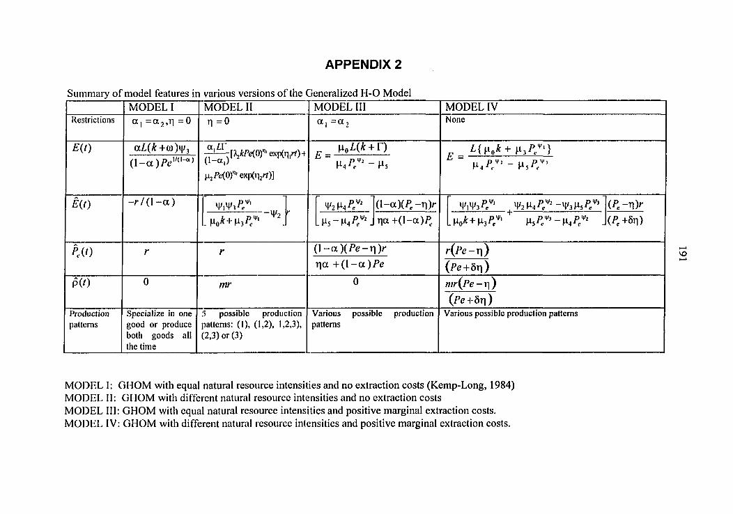
APPENDIX 2
Summary of model features in var ious vers ions of the General ized H-0 Model MODEL I MODEL II MODEL III MODEL IV
Restrictions a, =a2, i i =0 n = 0 a , =a2 None
E{t) aZ,(^+oj)xj/3 I r* -L[>,W'e(0)'"exp(ti,r^)+ U
expCrij^/)]
E{t)
(l-a)/'e"<'-"'
I r* -L[>,W'e(0)'"exp(ti,r^)+ U
expCrij^/)]
m - r / ( l - a ) m - r / ( l - a )
L U s - m C Jna+(l-a)^, J(/'.+5n)
PAO r r (l-a)(P<?-Ti)r
r | a + ( l - a ) P e r(Pe-r\)
(Pe+5ri)
p(0 0 mr 0 fnr(Pe-ri)
(Pe-i-5r\) Production
patterns
Specialize in one
good or produce
both goods all
the time
5 possible production
patterns: (1), (1,2), 1,2,3),
(2,3) or (3)
Various possible production
patterns
Various possible production patterns
MODEL I: GHOM with equal natural resource intensities and no extraction costs (Kemp-Long, 1984) MODEL II: GHOM with different natural resource intensities and no extraction costs MODEL III; GHOM with equal natural resource intensities and positive marginal extraction costs. MODEL IV: GHOM with different natural resource intensities and positive marginal extraction costs.