Coase, Hotelling and Pigou: The In iden e of a Carbon

Tax and CO2 Emissions

Geo�rey Heal

∗and Wolfram S hlenker

†

July 9, 2019

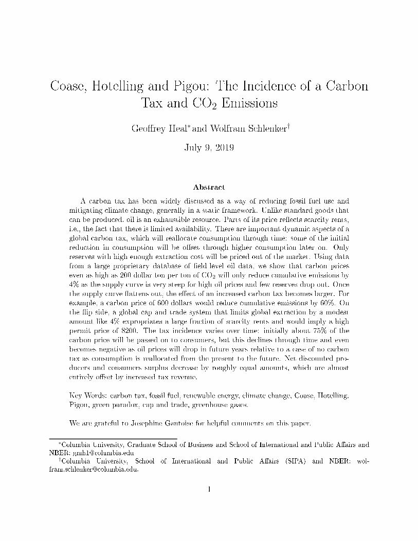
Abstra t

A arbon tax has been widely dis ussed as a way of redu ing fossil fuel use and

mitigating limate hange, generally in a stati framework. Unlike standard goods that

an be produ ed, oil is an exhaustible resour e. Parts of its pri e re�e ts s ar ity rents,

i.e., the fa t that there is limited availability. There are important dynami aspe ts of a

global arbon tax, whi h will reallo ate onsumption through time: some of the initial

redu tion in onsumption will be o�set through higher onsumption later on. Only

reserves with high enough extra tion ost will be pri ed out of the market. Using data

from a large proprietary database of �eld-level oil data, we show that arbon pri es

even as high as 200 dollar ton per ton of CO2 will only redu e umulative emissions by

4% as the supply urve is very steep for high oil pri es and few reserves drop out. On e

the supply urve �attens out, the e�e t of an in reased arbon tax be omes larger. For

example, a arbon pri e of 600 dollars would redu e umulative emissions by 60%. On

the �ip side, a global ap and trade system that limits global extra tion by a modest

amount like 4% expropriates a large fra tion of s ar ity rents and would imply a high

permit pri e of $200. The tax in iden e varies over time: initially about 75% of the

arbon pri e will be passed on to onsumers, but this de lines through time and even

be omes negative as oil pri es will drop in future years relative to a ase of no arbon

tax as onsumption is reallo ated from the present to the future. Net dis ounted pro-

du ers and onsumers surplus de rease by roughly equal amounts, whi h are almost

entirely o�set by in reased tax revenue.

Key Words: arbon tax, fossil fuel, renewable energy, limate hange, Coase, Hotelling,

Pigou, green paradox, ap and trade, greenhouse gases.

We are grateful to Josephine Gantoise for helpful omments on this paper.

∗Columbia University, Graduate S hool of Business and S hool of International and Publi A�airs and

NBER: gmh1� olumbia.edu

†Columbia University, S hool of International and Publi A�airs (SIPA) and NBER: wol-

fram.s hlenker� olumbia.edu.

1

There is almost universal agreement amongst e onomists who write about limate hange

that the introdu tion of a arbon tax would be a move in the right dire tion. The Brookings

Institution has a publi ation entitled �The Many Bene�ts of a Carbon Tax� (Morris (Adele

Morris n.d.)): the New York Times reported that �Republi an Group Calls for Carbon Tax�

(2/7/17), and the Finan ial Times noted that �Leading Corporations Support US Carbon

Tax� (6/20/17). The Carbon Pri ing Leadership Coalition

1

is a oalition of international and

national organizations and orporations dedi ated to promoting a arbon tax. The thinking

behind this is of ourse based on Pigou's work (Arthur Ce il Pigou 1920): the aim is to

internalize the external osts asso iated with the release of greenhouse gases by ombustion

of fossil fuels. Every environmental e onomi s text sees the internalization of external osts

as a ne essary step on the road the e� ien y. The Pigouvian framework is the default when

it omes to thinking about environmental poli y. But when it omes to thinking about

exhaustible resour es, whi h in lude all fossil fuels, there is another signi� ant framework,

introdu ed by Hotelling (Harold Hotelling 1931).

The point we are making in this paper is that these two frameworks lead to rather

di�erent on lusions when it omes to thinking about the e�e tiveness of a arbon tax.

Pigou emphasizes the impa t of a tax on substitution between ommodities, in this ase

between energy sour es. Hotelling on the other hand emphasizes the impa t of a tax on

an exhaustible resour e on the time-path of onsumption of that resour e. It an lead to

the substitution of future for present onsumption, so that less of the resour e is onsumed

by any date but the same amount is onsumed overall. One of the lear on lusions of the

Hotelling model of equilibrium in a resour e market is that if there is a substitute for the

resour e - think of renewable energy - available at a pri e in ex ess of the marginal extra tion

ost of the resour e, then all of the resour e will be onsumed eventually, and a arbon tax

an only hange this under rather stringent onditions. Carbon taxes appear less learly

bene� ial in the Hotelling framework than in the Pigouvian.

Ultimately, se tion 4 takes our model to data. We asses the impa ts on oil, oal and

gas supplies of arbon taxes using proprietary data on oil�eld ost stru tures from Rystad

Energy's UCube produ t and publi ly available data from the Energy Information Agen y.

A global tax of $50 per ton of CO2 would greatly redu e onsumption of oal and gas.

Espe ially oal will likely be pri ed out of the market under su h a tax.

The story is di�erent for rude oil. The oil market by itself is interesting, as re ent

estimates have argued onsuming all oil would use up the entire arbon budget that is left

1

www. arbonpri ingleadership.org

2

to keep the world within 2

◦C warming. S ar ity rents for oil are so high that only few oil

�elds will drop out of the market for moderate arbon taxes. For example, a arbon tax as

high as $200 will eliminate only 4% of oil �elds. An oil �eld be omes no longer pro�table

if the extra tion ost ex eed the ba kstop (or hoke) pri e minus the arbon tax. Lowering

the ba kstop pri e (e.g., heaper renewables) is equivalent to a arbon tax and might be

used in ombination with a arbon tax. About three quarters of tax will initially be passed

on to onsumers, but this in iden e de lines over time and even be omes negative as oil

onsumption is shifted from the present to the future under a arbon tax, de reasing the

pri e of oil by the end of the entury ompared to a ase without a tax. This makes the

politi al e onomy of a global arbon tax di� ult, as the osts are highest on immediate

users. In present value dis ounted terms, produ ers and onsumers roughly split the ost of

a arbon tax. The limited response in umulative oil onsumption implies that almost all

losses in onsumer and produ er surplus are o�set by higher tax revenue. Net exporters of

oil are predi ted to see welfare de lines, wile net importers see welfare in reases.

These empiri al results are a dire t result of exhaustible resour e models. After a brief

literature review in 1 we review the underlying theory in se tion 2. We start in se tion 2.1

with a basi model in whi h we explore the impa t of a arbon tax on the time pattern of use

of a fossil fuel fa ing ompetition from a renewable energy sour e whi h is a perfe t substitute

and is available at a pri e in ex ess of the marginal extra tion ost of the fuel, and show that

one of two out omes must hold: either the tax has no impa t on umulative onsumption of

the fossil fuel, though it does delay it; or it prevents any onsumption of the fuel at all. The

two energy sour es will never be used simultaneously. We then (se tion 2.2) modify the model

to re�e t the fa t that the renewable resour e is only an imperfe t substitute for the fuel.

In this ase we �nd that the fossil fuel and the renewable resour e are used simultaneously,

but the earlier basi on lusion still holds: a tax will either stop the onsumption of the fuel

altogether, or merely delay it. Se tion 2.3 looks at the onsequen es of introdu ing �xed

osts in the extra tion of fossil fuels, as well as variable osts. In this ase a arbon tax

may lead to a redu tion in the total onsumption of fossil fuels be ause the net revenues

from their sales no longer o�er an adequate return on the investment in the �xed ost. In

se tion 2.4 we onsider the more realisti , yet also more omplex, ase of multiple grades of

the fossil fuel di�ering in their extra tion osts. Here we �nd that a rise in a arbon tax may

delay the onsumption of the less expensive grades but eliminate from the market altogether

the more expensive grades, thereby redu ing greenhouse gas emissions. In se tion 2.5 we

look at the ase of a fossil fuel whose extra tion osts today are a fun tion of umulative

3

extra tion to date, a framework that leads to on lusions similar to those of se tion 2.4: total

extra tion may be redu ed. The overall on lusion is that there are two dimensions to the

impa t of a arbon tax: delaying the onsumption of fossil fuels, and eliminating expensive

fuels (expensive in either �xed or variable osts) from the market. Only the latter redu es

greenhouse gas emissions, and in some ases only the former me hanism will be e�e tive. In

se tion 3 we extend our model to onsider the impa t of a ap and trade system on emissions

from fossil fuels (an approa h based on the ideas of Coase (Ronald Coase 1960) about the

role of property rights in ontrolling externalities), and show that by �xing the allowable

quantity it attains the obje tive of redu ing emissions, but even modest quantity redu tions

imply a steep permit pri e. If permits are au tioned o� and not grandfathered, it has the

e�e t of expropriating the s ar ity rents asso iated with exhaustible fossil fuels.

1 Literature Review

The impa t of taxation on the pattern of resour e use was dis ussed in the 1970s by Partha

Dasgupta & Geo�rey Heal (1979) and Parth Dasgupta, Geo�rey Heal & Joseph Stiglitz

(1980) using the Hotelling framework. These papers pre-date on erns about limate hange

and greenhouse gases, and fo ussed on the impa t of taxation on the time pattern of resour e

use in a ontinuous-time in�nite-horizon ompetitive equilibrium. There was no spe i�

dis ussion of a arbon tax, with the fo us being on sales and pro�ts taxes and depre iation

and depletion regimes. These papers showed that, to quote, �there exists a pattern of taxation

whi h an generate essentially any desired pattern of resour e usage� (Dasgupta, Heal &

Stiglitz 1980). In other words, an appropriate system of taxation an produ e any time

pattern of use of a fossil fuel. But in all of these patterns, all of the fuel will be used up:

umulative use, and so emissions, will thus be the same in all. Only their distribution over

time will di�er from one ase to the other. This is onsistent with our �nding that in the

basi Hotelling model a arbon tax an hange the time pattern of fuel use but not alter the

total use and therefore not alter umulative greenhouse gas emissions.

A later literature on the �green paradox� (Hans-Werner Sinn 2015, Hans-Werner Sinn

2012, Mi hael Hoel 2012, Mi hael Hoel 2010, Sven Jensen, Kristina Mohlin, Karen Pittel &

Thomas Sterner 2015, Robert Cairns 2012) asks whether poli ies that are intended to redu e

greenhouse gas emissions ould in fa t have the opposite e�e t: ould they a tually promote

emissions? The literature arrives at a positive on lusion, noting that an expe tation of rising

taxes on fossil fuels will lead to an in rease in the rate at whi h they are used (Sinn 2012).

4

This is onsistent with earlier �ndings: Dasgupta Heal and Stiglitz �nd that �...the e�e ts of

tax stru ture on patterns of extra tion are riti ally dependent on expe tations on erning

future taxation.� They show that a sales tax that rises over time will lead to more rapid use

of an exhaustible resour e, and vi e versa, whi h is essentially the green paradox.

Reyer Gerlagh (2010) distinguishes between weak and strong green paradoxes: the weak

paradox o urs when poli ies in rease near-term arbon emissions, but not total emissions.

The strong paradox is used for ases when total emissions are in reased. In the models

onsidered in this paper there are no strong green paradoxes, and weak ones o ur only if

there is an in rease in the tax rate over time. Carbon taxes either have no impa t on total

emissions or redu e them. Ri k van der Ploeg & Cees Withagen (2010) and Ri k van der

Ploeg & Cees Withagen (2015) show that the anti ipation of a drop in the pri e of renewable

energy may also generate a green paradox, en ouraging the more rapid use of fossil fuels.

Hoel (2012) onsiders a model in whi h the ost of extra tion of a fossil fuel depends on the

umulative extra tion to date using the formulation of Geo�rey Heal (1976), and shows that

in this ase a arbon tax an redu e total greenhouse gas emissions. This is analogous to

our results in se tions 2.4 and 2.5, where we onsider multiple grades of a fossil fuel di�ering

in their extra tion osts.

2 Model

2.1 Basi Model

There is a sto k S0 > 0 of a fossil fuel, selling at a market pri e pt at date t in a ompetitive

market. Its marginal extra tion ost is onstant at m > 0 and its pri e pt is given by

pt = ht +m+ τ (2.1)

where τ is a per unit tax rate that must be paid on sales of the fuel. This is a arbon tax,

meaning that it is al ulated from the arbon released when the fuel is burned: it does not

depend on the value of the produ t. ht is the s ar ity rent or Hotelling rent on the fuel,

or its net pri e after extra tion and paying the tax, and we know that in a ompetitive

market equilibrium this will rise exponentially at the prevailing interest rate r (Dasgupta &

Heal 1979, hapter 6). Hen e

pt = h0ert +m+ τ (2.2)

5

In addition to the fossil fuel there is a renewable resour e available in unlimited amounts

at a marginal and average ost of R > m. This is a perfe t substitute for the fossil fuel (it is

a �ba kstop te hnology� in the terminology of Dasgupta & Heal (1979)), so that if the fuel

is onsumed we must have

pt ≦ R (2.3)

Demand for the fuel is given by the demand fun tion D (pt). We are interested in the

ompetitive equilibrium dynami s of pri es and demand for the fuel, and how these are

a�e ted by the arbon tax. We know that the market pri e of the fuel will rise exponentially

away from m+ τ at rate r, as given in (2.2), and that pt = h0ert +m+ τ ≦ R if the fuel is

sold.

Proposition 1. Assuming perfe t substitutability between the fossil fuel and renewable en-

ergy, a dynami ompetitive equilibrium with a arbon tax τ , m + τ < R, is hara terized

by the equations (2.4) and (2.5). These determine the initial rental rate h0 and the date T

at whi h pt = R and the fossil fuel is exhausted. There is no interval of time over whi h

the fossil fuel and the renewable energy sour e are both used. If the tax rate is raised to

τ ′ > τ, m+ τ ′ < R, then the above remains true so that total fossil fuel onsumption is not

hanged. Su h a tax in rease de reases the initial rental rate h0 and in reases the date T at

whi h the fossil fuel is exhausted. If the tax is so high that m+ τ > R then the fossil fuel is

never onsumed.

Proof. For all markets for the fuel to lear it is ne essary and su� ient that the time T at

whi h pt = R and the initial Hotelling rent h0 satisfy the following two equations:

ˆ T

0

D (pt) dt =

ˆ T

0

D(h0e

rt +m+ τ)dt = S0 (2.4)

and

pT = h0erT +m+ τ = R (2.5)

Equation (2.4) tells us that demand equals supply umulatively over time, and equation

(2.5) tells us that the pri e of the fuel never ex eeds that of the renewable energy sour e

and be omes equal to it just as the total amount of the fossil fuel is used up. Continuity of

the pri e over the transition from the fossil fuel to the renewable energy sour e is ne essary

for ompetitive equilibrium: if there were a jump in pri e sellers would withhold supply in

anti ipation of apital gains, meaning that the path with a jump was not an equilibrium.

These two equations an be solved for the two unknowns h0 and T, the initial resour e rent

6

and the date at whi h the resour e is exhausted and the e onomy transits to renewable

energy. Equation (2.5) gives

h0 = (R−m− τ) e−rT(2.6)

and we an use this in equation (2.4) to solve for T.

It is lear that as long as m + τ < R the ompetitive equilibrium will involve a period

[0, T ] during whi h only the fossil fuel is onsumed and then a period from T onwards during

whi h only renewable energy is used, and that over the interval [0, T ] all of the fossil fuel

will be onsumed.

An alternative is that the tax τ is so high that m+ τ > R, in whi h ase the fossil fuel

will never be onsumed.

2

Hen e we on lude that a arbon tax either delays onsumption

of the fossil fuel but does not hange total umulative onsumption, or alternatively redu es

the onsumption of the fossil fuel to zero. There is no intermediate ase in whi h the tax

redu es the total onsumption of the fossil fuel but not to zero.

We an use (2.6) in (2.4) to get

ˆ T

0

D([R −m− τ ] er(τ−T ) +m+ τ

)= S0 (2.7)

and from this we an ompute omparative stati s with respe t to the tax rate τ . It is lear

from this that ∂T/∂τ > 0 and from (2.6) that ∂h0/∂τ < 0, as asserted in the proposition.

This means that an in rease in the arbon tax rate will extend the e onomi life of the

fossil fuel, redu ing its onsumption rate at any date, and will redu e the rent it earns at all

dates.

There is a simple intuition behind this result. Suppose to the ontrary that at time T

we have pT = R and

´ T

0D (pt) dt < S0, so that a sto k of unsold fuel remains. Its pri e is

now onstant so that the rate of return to holding it is zero. But agents will only hold this

sto k if it o�ers a return equal to the available elsewhere - r - so the sto k will be dumped

on the market, meaning that the market was not originally in equilibrium. Hen e there

annot be a market equilibrium in whi h sto ks of the fossil fuel remain unsold, as long as

m+ τ < R. If the reverse inequality holds then the fuel is valueless and sto ks will never be

pur hased in the �rst pla e. Provided that the marginal extra tion ost plus tax is less than

the pri e of the renewable energy sour e, all of the fossil fuel will be onsumed, as it will

always be pro�table to extra t and sell it. No hange in the tax rate - as long as it satis�es

2

See also Hoel (2012) for a dis ussion of this ase: he refers to su h a tax as a �high tax.�

7

the ondition m+ τ < R - will alter this. Another way of thinking about this is that with a

normal produ ed good, a tax would redu e the net pri e re eived by the maker and redu e

output along the supply urve. With an exhaustible resour e there is no supply urve: the

resour e is there whatever the pri e and is pro�table as long as m+ τ < R.

2.2 Imperfe t Substitutability

Given what we observe in the world around us, the results above seem surprising: we see

both renewable energy and fossil fuels in the market at the same time, rather than the

abrupt swit h from one to the other that the model predi ts. There are several possible

reasons for this dis repan y. Prin ipal amongst them is that we have assumed that fossil

fuels and renewable resour es are perfe t substitutes, so that demand swit hes ompletely

from one to the other as the ordering of their pri es hanges. In reality this is not the ase:

renewable energy is intermittent, whi h is a disadvantage relative to fossil energy, but is

lean, produ ing no pollutants that damage the lo al environment and no greenhouse gases.

Be ause of these fa tors we an imagine situations where renewable energy is used even if

it is more expensive (situations where there is a need to redu e lo al pollution, or to redu e

greenhouse gas emissions) and onversely situations where a fossil energy su h as natural

gas is used even though it is more ostly (for example gas is used to ba k up intermittent

renewable energy). To try to apture these possibilities, we now modify the demand for fossil

fuels to show that it depends not only on its own pri e pt but also on the pri e of renewable

energy R: D (pt, R) , ∂D/∂R > 0. This admits the possible o-existen e of both energy

sour es in the market simultaneously, with demand transferring from one to the other as the

pri e di�eren e hanges. We assume the demand fun tion to have a � hoke pri e� p (R) su h

that demand for the fossil fuel falls to zero when its pri e rea hes p (R). So D (p (R) , R) = 0.

Obviously the hoke pri e depends on the pri e of the substitute. In the previous analysis

p (R) = R. Clearly we expe t that p (R) is in reasing in R.

It is still the ase that in equilibrium the pri e of the fossil fuel will be given by 2.2, with

the Hotelling rent rising exponentially at the interest rate. For all markets for the fuel to

lear it is now ne essary and su� ient that the time T at whi h the pri e of the fuel equals its

hoke pri e, pT = p (R), and the initial Hotelling rent h0 satisfy the following two equations:

ˆ T

0

D (pt) dt =

ˆ T

0

D(h0e

rt +m+ τ)dt = S0 (2.8)

pT = h0erT +m+ τ = p (R) (2.9)

8

These equations are the same as 2.4 and 2.5 ex ept that the pri e of the renewable resour e

has been repla ed by the hoke pri e, a fun tion of the pri e of the renewable resour e.

3

As

in the earlier ase, these two equations have two unknowns, h0 and T , and an be solved for

these.

This framework leads to similar on lusions to the previous one, ex ept that the transition

from the fossil fuel to the renewable resour e is now smooth rather than abrupt.

Proposition 2. Assuming imperfe t substitutability between the fossil fuel and renewable

energy re�e ted in the demand fun tion D (pt, R) with hoke pri e p (R), a dynami ompet-

itive equilibrium with a arbon tax τ , m + τ < p (R), is hara terized by the equations 2.10

and 2.11. These determine the initial rental rate h0 and the date T at whi h pt = p (R) and

the fossil fuel is exhausted. If the tax rate is raised to τ ′ > τ, m+ τ ′ < p (R), then the above

remains true so that total fossil fuel onsumption is not hanged. If the tax is so high that

m+ τ > p (R) then the fossil fuel is never onsumed.

Proof. For all markets for the fuel to lear it is ne essary and su� ient that the time T

at whi h pt = p (R) and the initial Hotelling rent h0 satisfy the following two equations

analogous to 2.4 and 2.5:

ˆ T

0

D (pt, R) dt =

ˆ T

0

D(h0e

rt +m+ τ, R)dt = S0 (2.10)

pT = h0erT +m+ τ = p (R) (2.11)

The rest of the argument is as in Proposition 1, ex ept that it is now possible that the fossil

fuel and renewable energy are used simultaneously.

The important point here is that even with imperfe t substitutability and the o-existen e

of both produ ts in the market, a arbon tax will not a�e t the total umulative onsumption

of the fossil fuel. The intuition is exa tly as before. Renewable energy may be substituted

for the fossil fuel, but this will merely spread out the onsumption of the fuel over time and

will not redu e total onsumption. We an also show, as in Proposition 1, that an in rease

in the tax rate will in rease T and lower the initial rent h0.

3

Depletion of the fuel before its hoke pri e is rea hed is in onsistent with pro�t-maximization.

9

2.3 Fixed Costs of Extra tion

So far we have assumed that all the osts of extra ting the fossil fuel are variable osts,

with a marginal extra tion ost of m > 0. Suppose in addition that there is a �xed ost

F > 0 that must be in urred before the fuel an be extra ted at a marginal ost of m. This

ould be the ost of �nding and developing an oil or gas �eld, a ost that in pra ti e an be

substantial. Could this alter our on lusions?

In this ase the fuel will only be produ ed if the pri e is high enough to over the tax,

extra tion ost and �xed ost. The time path of the fuel pri e will still be given by 2.2, so

now we require that

ˆ T

0

(pt −m− τ) dt =

ˆ T

0

h0ert ≥ F (2.12)

Market learing onditions are still given by equations 2.10 and 2.11, and the onstraint 2.12

introdu es the possibility that an in rease in the tax rate ould make it impossible to satisfy

the onstraint 2.12. Integrating 2.12 gives

erT ≥rF

h0+ 1 (2.13)

and in this inequality F and r are exogenously given and T and h0 are given by market

learing equations 2.10 and 2.11. It is lear that these values of the variables and parameters

need not satisfy 2.13. The introdu tion of �xed osts in the extra tion te hnology therefore

gives another me hanism via whi h a arbon tax might prevent the extra tion of the fossil

fuel, but on e again if the fuel is extra ted at all then it will all be extra ted. If there is an

initial tax rate at whi h extra tion is pro�table - i.e. 2.13 is satis�ed - but after extra tion

has begun the tax is in reased to a point where this is no longer true, extra tion will ontinue

provided that m+ τ < p (R).

2.4 Multiple Grades of Fossil Fuel

Another ase of interest is that of multiple sour es of the fossil fuel, with di�erent extra tion

osts. Suppose we modify the model of se tion 2.1 so that there are I di�erent fuel sour es

ea h with marginal extra tion ost mi and let them be numbered in in reasing order of

extra tion osts, so that m1 < m2 < m3 < ..... < mI and further assume that mI < R so

all are less expensive than the renewable resour e. (Others will never be used and an be

negle ted.) The initial sto k of the i− th fuel is Si,0. The ompetitive equilibrium out ome

is that there exist dates Ti, i = 1, 2, ....I, Ti < Ti+1, and initial rents h0,i, i = 1, 2, ..., I su h

10

that for all i,

pi,t = mi + τ + hi,0ert, Ti−1 ≤ t ≤ Ti (2.14)

and

ˆ Ti

Ti−1

D (pi,t) dt = Si,0 (2.15)

So ea h grade of fuel i is used over the interval Ti−1 ≤ t ≤ Ti and is used only during this

interval and is used up by the end of this interval. The least expensive fuel is used up �rst

and the most expensive last (Dasgupta & Heal 1979, page 172 se tion (iii)). This referen e

also shows that the pri e moves ontinuously so that

pi,Ti= mi + τ + hi,0e

rTi = pi+1,Ti= mi+1 + τ + hi+1,0e

rTi ∀i (2.16)

and we must have the last pri e of the fuel equal to that of renewable energy:

pI,TI= R (2.17)

In this ase the impa ts of a arbon tax are essentially the same as before: provided that

mi + τ < R, a tax in rease will merely delay the onsumption of the fossil fuel, but will not

alter umulative onsumption. However if there are many grades of fossil fuel with di�erent

osts, it is possible that the more expensive of them have osts lose to R, in whi h ase a

tax in rease ould lead to mj + τ > R for some grade j, in whi h ase fuel of grade j will not

be produ ed and umulative emissions will fall. Be ause of the existen e of multiple grade

of fuel we no longer have the earlier all-or-nothing impa t of a tax rise: it an now lead to

the elimination of some but not all of greenhouse gas emissions by pushing out of the market

the more ostly fossil fuels.

Clearly we an ombine the results of proposition 2 of se tion 2.2 on imperfe t substi-

tutability with those of this se tion to onsider the e�e t of taxation when there are multiple

grades of fossil fuel, all of whi h are perfe t substitutes for ea h other but imperfe t sub-

stitutes for renewable energy, as in se tion 2.2. Be ause the di�erent grades are perfe t

substitutes for ea h other, they must sell at the same pri e, whi h means that only one an

be on the market at any time. As in se tion 2.2 there is a hoke pri e p (R) for the fuel (the

same for all grades as they are perfe t substitutes). Now we have an equilibrium in whi h

di�erent grades of the fuel are exhausted sequentially from least to most expensive, with the

use of some of them overlapping with that of the renewable energy sour e. So an equilibrium

is hara terized by dates Ti, i = 1, 2, ....I, Ti < Ti+1, and initial rents h0,i, i = 1, 2, ..., I su h

11

that for all i,

pi,t = mi + τ + hi,0ert, Ti−1 ≤ t ≤ Ti (2.18)

and

ˆ Ti

Ti−1

D (pi,t) dt = Si,0 (2.19)

and ontinuity of pri es with the last pri e of the fuel being its hoke pri e:

pi,Ti= mi + τ + hi,0e

rTi = pi+1,Ti= mi+1 + τ + hi+1,0e

rTi ∀i, pI,TI= p (R) (2.20)

In this ase the tax will lead to lower emissions at any date and to lower emissions in

total over time if it displa es one or more of the expensive grades of the fuel.

2.5 Extra tion-Dependent Costs

The last ase we will look at is that of a fuel whose extra tion ost is a fun tion of umulative

extra tion to date. The motivation for su h an assumption is lear: there are many grades of

the resour e that vary in extra tion osts, and the lowest ost grades, those that are easiest

to extra t, are removed �rst, driving up osts as extra tion in reases. This is similar to the

ase onsidered in the last se tion, ex ept that the problem is formulated in a ontinuously

variable framework and there is an expli it dependen e of urrent osts on past extra tion,

implying that urrent poli ies an alter future osts and this needs to be taken into a ount

in de iding how mu h to extra t now. We assume that the resour e extra tion at date t is

given by Et ≥ 0, and that umulative extra tion is denoted zt =´ t

0Eκdκ. The total amount

of the resour e is z, so zt ≤ z. As before R denotes the ost of a renewable substitute for the

resour e. Extra tion osts at time t, ct, are given as follows:

ct = g (zt) , g (zt) ≤ R : ct = R, g (z) > R : g′ (z) =dg

dz> 0 (2.21)

So the ost of extra tion is given by the in reasing fun tion g (z) as long as it is less than

the ost of the renewable resour e and after that only the renewable resour e is used. This

is the formulation used in Heal (1976), and also in Hoel (2012), who also studies the e�e t

of a arbon tax in this framework, fo ussing on the onsequen es of a tax that hanges over

time.

In a ompetitive equilibrium there are potentially two regimes: in the �rst the resour e is

extra ted and its extra tion ost is less than or equal to the ost of the renewable resour e,

12

whi h is not used, and in the se ond the resour e is either exhausted (the ase when g (z) ≤

R) and only the renewable resour e is used, or alternatively the ost of the resour e ex eeds

that of the renewable resour e and again only the latter is used. The �rst regime will exist

as long as g (0) < R.

As before let the arbon tax rate be τ , so that the total ost of bringing the resour e to

market is c (zt) = g (zt) + τ . Let p be the market pri e of the resour e and po the pri e of a

generi output good produ ed from the resour e. Then we an establish the following

Proposition 3. The market pri e of the resour e in the �rst regime satis�es the following

equation

p

p= δ

(p− c

p

)+

popo

c

p(2.22)

Proof. An extension of the proof in (Heal 1976).

This proposition has a simple interpretation. The resour e pri e rises at a rate whi h is

a weighted average of the dis ount rate and the rate at whi h the output pri e is in reasing,

where the weight on the dis ount rate is the fra tion of the pri e made up of rent and the

weight on the rate of hange of the output pri e is the fra tion of pri e made up of osts. So if

extra tion osts are zero we have the pure Hotelling ase, and if extra tion osts are non-zero

but onstant, as in se tion 2.1, the output pri e is onstant and we have the rent rising at

the dis ount rate. The resour e pri e will rise a ording to this rule until either the resour e

is exhausted or the pri e rea hes that of the renewable resour e and so iety swit hes to that:

if this happens before resour e exhaustion then unused sto ks of the resour e remain.

In this ontext the impa t of a arbon tax is easily understood: it raises the extra tion

ost c (zt). The fossil fuel will ease to be used as soon as its ost in luding tax ex eeds that

of the renewable resour e, i.e. as soon as

c (zt) = g (zt) + τ ≥ R (2.23)

or

z ≥ z∗ = g−1 [R− τ ] (2.24)

As g is in reasing, so is g−1, so an in rease in the tax rate τ may redu e z∗ the level of

umulative extra tion at whi h the fossil resour e eases to be ompetitive. There are two

ases: if g (z) + τ < R then the tax has no impa t on the amount of the fossil fuel used,

as it is not su� ient to raise the extra tion ost above the ost of the renewable resour e.

13

If however g (z) + τ > R then the tax does redu e total onsumption of the fossil resour e,

setting a bound on umulative extra tion at z, g (z) = R− τ, z < z.

3 Cap and Trade

The widely- onsidered alternative to a arbon tax is a ap-and-trade (C&T) system, and

next we review the operation of su h a system in the ontext of a Hotelling model. We �rst

work with a simpli�ed version of the basi model of se tion 2.1, and then onsider the impa t

of various re�nements. There is a sto k S0 > 0 of a fossil fuel, selling at a market pri e pt

at date t in a ompetitive market. There is no arbon tax and we take marginal extra tion

osts to be zero for the moment. Hen e the pri e satis�es pt = p0ertwhere the initial pri e

p0 satis�esˆ

∞

0

D(p0e

rt)= S0 (3.1)

Consumption of a unit of the fossil fuel emits one unit of greenhouse gas, and an environ-

mental authority imposes a ap of K0 units on the total umulative emissions of greenhouse

gases. This implies that

ˆ

∞

0

D(p0e

rt)≤ K0 (3.2)

This formulation means that permits an be banked, that is arried over freely from one

period to the next, so that the onstraint is on total umulative emissions and not on period-

by-period emissions. Clearly one of the equations 3.1 and 3.2 is redundant: if S0 < K0 then

the emissions onstraint is redundant, and in the more likely ase that the reverse is true,

namely K0 < S0, some of the fossil fuel will be left unused and the binding onstraint will be

that

´

∞

0D (p0e

rt) = K0. In this ase the s ar ity rent asso iated with the onstraint 3.1 will

be zero, but a positive s ar ity rent will be asso iated with the emissions onstraint 3.2. So

in a market equilibrium, the pri e of the fossil fuel will be zero but there will be a pri e for

emissions permits. As su h permits are an exhaustible resour e, their pri e will move exa tly

as the pri e of su h a resour e. Letting the permit pri e be rt, this will satisfy rt = r0ertand

´

∞

0D (r0e

rt) = K0. The key point to understand here is that the presen e of a binding ap

on emissions from the fossil fuel redu es the rent on the resour e to zero and all of the rent

is now aptured by the permit pri e. So the agen y that au tions permits now aptures all

of the s ar ity rent that previously a rued to the resour e owners. Finan ially speaking,

the resour e has been fully expropriated.

Now suppose that as in se tion 2.1 there is a positive ost m > 0 to extra ting the fossil

14

fuel. In the absen e of a ap and trade system, Proposition 1 would hold, and the rent on

the resour e would rise at the interest rate, with the sto k of the resour e being exhausted

at exa tly when the pri e �rst equals that of the ba kstop te hnology if there is one. But

if as in the previous paragraph there is a ap and trade system with the ap on emissions

tight enough that not all of the fossil fuel an be onsumed, matters are again more omplex.

Letting rt be as before the pri e of a permit at time t, in selling a unit of fossil fuel at time

t the owner in urs osts of m to extra t it and rt to buy a permit, so that her ost is m+ rt.

Permits are as before an exhaustible resour e, so that their pri e will rise at the interest rate,

so that the resour e seller's osts move over time as m+ r0ert, where the initial permit pri e

r0 will as before be hosen so that

´

∞

0D (r0e

rt) = K0. On e again the s ar ity rent on the

fossil fuel is redu ed to zero and is repla ed by the s ar ity value of the emission permits, so

again the fuel is e�e tively expropriated.

If there is heterogeneity in extra tion ost mi among reserves (se tion 2.4), owners of

the heaper reserves will retain some of their rents, as the pri e of the permit is given by

reseve owner who is on the margin between produ ing or not produ ing. As we will show in

the empiri al se tion below, the onvexity of the marginal ost urve implies that a modest

redu tion in umulative oil onsumption would expropriate a signi� ant share of the s ar ity

rents.

Finally we onsider a more omplex ase: above the emissions permits were in�nitely

bankable, that is ould be used at any point in time. In reality permits generally have

a �nite life, so we analyze the out ome in this ase. To be pre ise, we assume that the

environmental authority issues two sets of permits: one set are valid from time zero to time

T , and the others from T onwards for ever. Permits issued at time zero lose all value at

time T , and over in total K0 units of emissions. The permits issued at date T over a

total of KT units of emissions. We will take the marginal extra tion ost to be zero, so

that m = 0. Let q∗t be the ompetitive equilibrium onsumption of the fuel at date t in

the absen e of any poli y interventions, i.e. with no ap and trade system or tax, and let

QT0 =´ T

0q∗t dt, Q

∞

T =´

∞

Tq∗t dt. We will for the moment take it that K0 = ∞, and KT < Q∞

T ,

so that there is no onstraint on emissions from zero to T and the ap on emissions after

T is less than would be onsumed on the ompetitive path from that date onwards. In

this situation, what is the ompetitive path of onsumption (and emissions) from zero to T ,

assuming that all players in the market at date zero are aware of the ap that omes into

e�e t at T ? The total amount of fuel available for onsumption over [0, T ] is S0 −KT and

the ompetitive path is one on whi h just this amount is onsumed over that time period.

15

So the pri e path pt satis�es

ˆ T

0

D(p0e

rt)dt = S0 −KT (3.3)

(p0 is the only unknown in this equation, whi h we assume to have a solution.) In this ase

the amount left at time T is exa tly equal to the ap under the C&T system and the pri e

of the fuel post-T will rise at the interest rate as in a ompetitive equilibrium. There will be

a drop in onsumption and a jump in the pri e at T , whi h will be fully anti ipated but will

not give rise to arbitrage as no fuel an be transferred from before to after T be ause of the

ap.

Now suppose that K0 < S0 − KT so that the solution we have just des ribed is not

permitted. In the earlier period [0, T ] the permit onstraint is binding, not the resour e

onstraint. In this ase the resour e pri e will be zero and the permit pri e will be positive.

Permits for the period [0, T ] are an exhaustible resour e over that period, and their ompet-

itive pri e will rise at the interest rate from 0 to T from an initial level su h that the sto k

K0 of [0, T ] permits is just exhausted at T . On e again the C&T system transfers value

from the resour e market to the permit market. After T the emissions onstraint is again

binding, as KT < S0 − K0, so that again the pri e of the resour e is zero and all s ar ity

rent is aptured in the permit market.

4 Numeri al Analysis: Extra tion Costs and Tax Rates

To get as sense of the empiri al signi� an e of our analysis and understand the impa t of a

arbon tax on fossil fuels, we need to know how mu h CO2 ea h type of fuel releases when

burned. Table 1 gives this data for oal, gas and rude oil. For one metri ton of oal (MT),

one million BTU of gas (MMBTU), and one barrel of oil (BBL), it shows how mu h CO2

is emitted when this is burned.

4

There is a range of estimates for how mu h CO2 will be

released when one barrel of oil is burned. It depends on the exa t omposition of the fuel

and the pro ess by whi h it is burned. We give the baseline number underlying the Canadian

arbon tax. The table also gives the urrent US pri e in dollars, and the amount that a $50

4

The exa t arbon ontent depends on the omposition of the fuel. We quote some estimates to

highlight the order of magnitude. For gas see https://www.eia.gov/tools/faqs/faq.php?id=73&t=11,

for oal see https://www.eia.gov/ oal/produ tion/quarterly/ o2_arti le/ o2.html, and for gasoline

see https://www. anada. a/en/department-�nan e/news/2018/10/ba kgrounder-fuel- harge-rates-in-listed-

provin es-and-territories.html

16

arbon tax would raise per unit of the fuel.

Looking at the numbers in Table 1, it is very lear that the e�e t of a $50 arbon tax

is potentially mu h greater in relative terms on oal and gas than on oil: for oal the tax

is $143 and the pri e is around $50, so that the tax is almost three times the pri e. The

equivalent tax on natural gas is $2.65, while the wholesale pri e that is just under $3, i.e.,

the tax almost equals the pri e. For oil, however, the tax is about $17.6 and the market

pri e around $65, i.e., the tax equals around a third of the urrent pri e.

All three of these fuels are exhaustible resour es, so that the earlier analysis is appli able

to all of them. We therefore need to assess whether a arbon tax will in rease the MEC -

regarding the tax as a part of the MEC - to the point where it is unpro�table to extra t the

resour e. For oal, adding the tax would roughly quadruple the urrent pri e, very likely

deeming it un ompetitive. We would expe t a $50 per ton arbon tax to put the thermal

oal industry out of business in the US. For natural gas, the answer will also generally be

a�rmative. It is widely assumed in the oil and gas industry that most gas produ ers are

losing money at the urrent pri e of $3 per MMBTU, implying that average osts ex eed

$3, though the marginal osts of gas are generally low. One sour e gives operating osts

as 34% of total osts for an average shale gas �eld, and if this �eld is breaking even at $3

then we have an operating or marginal ost of $1.

5

These �elds would be unpro�table at

a $50 per ton arbon tax. In those few ases in whi h gas is an unintended byprodu t of

oil produ tion (�asso iated gas�), one ould make an argument that the gas e�e tively has a

zero marginal ost. About 20% of US gas is asso iated gas

6

so about 20% would be immune

from the e�e ts of a $50 arbon tax.

Oil is a more omplex and interesting ase. The world pri e (the pri e of Brent marker

rude) is in the mid $60s per barrel, and the US marker rude, West Texas Intermediate

(WTI) is in the high $50s (as of 6/28/2019). A $50 arbon tax would imply a per-barrel

harge that is roughly one third of the urrent pri e.

4.1 Oil Market

Our empiri al simulation of optimal oil extra tion over time requires three important inputs:

the marginal extra tion ost of various oil �eld (produ er side), the pri e of the ba kstop

te hnology or hoke pri e (R in the modeling se tions above), and the demand fun tion

(demand elasti ity).

5

http://www.insightenergy.org/system/publi ation_�les/�les/000/000/067/original/RREB_Shale_Gas_�nal_20170315_published.pdf?1494419889

6

See https://www.forbes. om/sites/jude lemente/2018/06/03/the-rise-of-u-s-asso iated-natural-gas/#73e287 04bd7

17

For the produ tion side, we use the proprietary data from Rystad Energy, a prominent

sour e of mi ro-level data set of various oil �elds around the globe. For example, it has

re ently been used by John Asker, Allan Collard-Wexler & Jan De Loe ker (2019) to study

the misallo ation of oil produ tion around the world. The data set gives estimates for roughly

15,000 dis overed and 27,000 undis overed oil �assets� ' around the world. An asset is the

smallest geographi s ale in the data. For example, portions of an oil �eld an be owned

by several �rms, and ea h one of the owners will be listed as separate asset. Importantly

for us, Rystad gives estimates of a breakeven pri e for ea h asset. For dis overed oil �elds,

this only in ludes the variable operating ost as marginal ost, as investments in exploration

and development are sunk. For undis overed assets, it does in lude these osts, as initial

investments are required to a ess these assets.

7

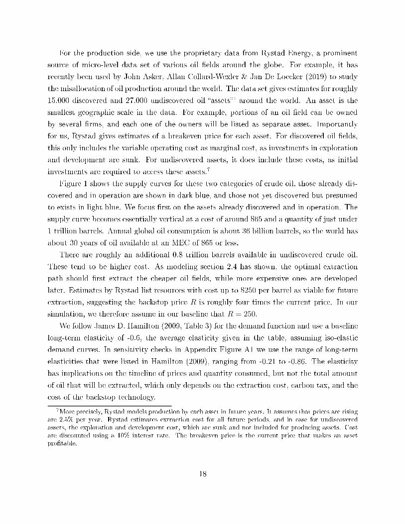
Figure 1 shows the supply urves for these two ategories of rude oil, those already dis-

overed and in operation are shown in dark blue, and those not yet dis overed but presumed

to exists in light blue. We fo us �rst on the assets already dis overed and in operation. The

supply urve be omes essentially verti al at a ost of around $65 and a quantity of just under

1 trillion barrels. Annual global oil onsumption is about 36 billion barrels, so the world has

about 30 years of oil available at an MEC of $65 or less.

There are roughly an additional 0.8 trillion barrels available in undis overed rude oil.

These tend to be higher ost. As modeling se tion 2.4 has shown, the optimal extra tion

path should �rst extra t the heaper oil �elds, while more expensive ones are developed

later. Estimates by Rystad list resour es with ost up to $250 per barrel as viable for future

extra tion, suggesting the ba kstop pri e R is roughly four times the urrent pri e. In our

simulation, we therefore assume in our baseline that R = 250.

We follow James D. Hamilton (2009, Table 3) for the demand fun tion and use a baseline

long-term elasti ity of -0.6, the average elasti ity given in the table, assuming iso-elasti

demand urves. In sensitivity he ks in Appendix Figure A1 we use the range of long-term

elasti ities that were listed in Hamilton (2009), ranging from -0.21 to -0.86. The elasti ity

has impli ations on the timeline of pri es and quantity onsumed, but not the total amount

of oil that will be extra ted, whi h only depends on the extra tion ost, arbon tax, and the

ost of the ba kstop te hnology.

7

More pre isely, Rystad models produ tion by ea h asset in future years. It assumes that pri es are rising

are 2.5% per year. Rystad estimates extra tion ost for all future periods, and in ase for undis overed

assets, the exploration and development ost, whi h are sunk and not in luded for produ ing assets. Cost

are dis ounted using a 10% interest rate. The breakeven pri e is the urrent pri e that makes an asset

pro�table.

18

It should be emphasized that we are modeling the longterm dynami s of oil pri es. We

abstra t from short-term in�uen es, e.g., politi al unrest or demand sho ks. For example,

Soren T. Anderson, Ryan Kellogg & Stephen W. Salant (2018) have shown that on e an

oil �eld is set up for produ tion, it is often ostly to halt produ tion, violating one of

the assumptions of the lassi al Hotelling model that oil an be produ ed at any time.

Development of new wells respond to pri es, but produ tion of existing wells do so to a

lesser degree. This an lead to di�erent short-term dynami s. Sin e we are interested in the

optimal exploration path over the next 100 years under various arbon taxes, we abstra t

from these short-term in�uen es.

Combining the three data sets allows us to onstru t the optimal extra tion pro�le over

time. We follow the theory of reserves with heterogenous ost of se tion 2.4. We know

that the most ostly reserves will be used last and that the pri e in the �nal period has to

equal the ost of the ba kstop R = 250. This allows us to solve the problem ba kwards,

going from the mostly ostly to the least ostly reserves (whi h will produ e �rst in time).

We use a daily time step.

8

Rents have to rise at the rate of interest for reserves with the

same marginal ost. On e reserves of a parti ular quality (marginal ost) are exhausted, the

pri e stays ontinuous, but the rent h() jumps dis ontinuously by the di�eren e in marginal

extra tion ost. The exa t steps of this ba kward analysis are given in Appendix se tion A1.

There is one free parameter in our simulations. The parameter α of the iso-elasti demand

fun tion qt = αpηt . On e we �x the paremeter, we simulate the problem ba kwards to obtain

estimates for both the equilibrium pri e p2019 and quantity q2109. We iterate over α to mat h

urrent global onsumption at 100 million barrels a day. Sin e we have two equilibrium

out omes but only one parameter, there is an impli it test of the other parameter assumptions

of the model: they should give us a pri e p2019 that mat hes the urrent equilibrium pri e.

For our baseline assumption, i.e. a demand elasti ity of −0.6, interest rate of r = 0.03 and

ba kstop pri e of R = 250, the equilibrium pri e of 63.22 losely aligns with urrent market

pri e of oil. Using parameters from the literature gives results that are internally onsistent.

On the other hand, if we hoose the lower bound of the elasti ities η = −0.21, the simulated

pri e of 80.42 seems too high, while the upper bound of the elasti ities η = −0.86, the

simulated pri e of 52.69 seems too low.

9

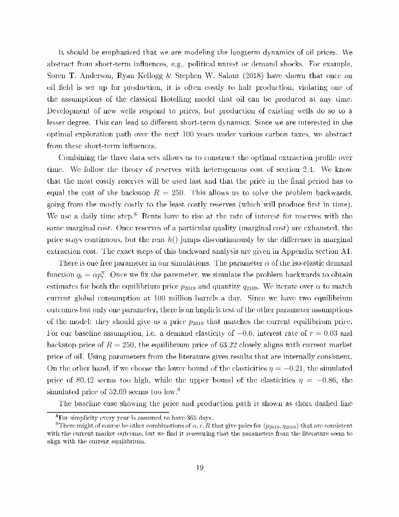
The baseline ase showing the pri e and produ tion path is shown as short dashed line

8

For simpli ity every year is assumed to have 365 days.

9

There might of ourse be other ombinations of α, r,R that give pairs for (p2019, q2019) that are onsistentwith the urrent market out ome, but we �nd it reassuring that the parameters from the literature seem to

align with the urrent equilibrium.

19

( arbon tax = 0) in Figure 2. The dashed red line shows the in reasing pri e path over time,

rising from 63.22 a barrel to 250 when the pri e equals the ba kstop pri e in the �nal period

2097, at whi h point the produ tion quantity, shown in blue, falls to zero. Demand after

2097 would only ome from the ba kstop te hnology (i.e., renewables). Alternative s enarios

for arbon taxes ranging from $50 to $400 per ton of CO2 are added as well. Higher taxes are

shown in a darker shade of blue and red as shown in the legend. Not surprisingly, a arbon

tax raises the pri e in 2019, as a portion of it is passed on to onsumers. The higher pri e

implies lower produ tion and lower resour e rents h() to produ ers. These lower resour e

rents now rise at the rate of interest, implying that oil pri es grow more slowly than in the

baseline ase under no arbon tax. Interestingly, there is a point towards the end of the

entury when pri es under the arbon tax be ome lower than in the baseline ase without

a arbon tax. The reason is that the arbon tax shifts some of the produ tion from the

present to later periods, implying a lower equilibrium pri e and higher produ tion quantity.

As shown in the theoreti al se tion, the lifetime is extended under a arbon tax, i.e., the

�nal period will be 2100 under a $50 arbon tax, and 2107 under a $400 arbon tax, when

produ tion again falls to zero.

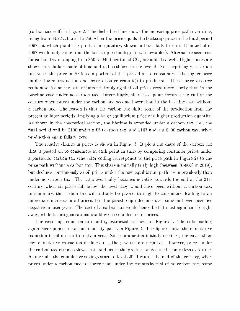
The relative hange in pri es is shown in Figure 3. It plots the share of the arbon tax

that is passed on to onsumers at ea h point in time by omparing onsumer pri es under

a parti ular arbon tax (the olor oding orresponds to the pri e path in Figure 2) to the

pri e path without a arbon tax. This share is initially fairly high (between 70-80% in 2019),

but de lines ontinuously as oil pri es under the new equilibrium path rise more slowly than

under no arbon tax. The ratio eventually be omes negative towards the end of the 21st

entury when oil pri es fall below the level they would have been without a arbon tax.

In summary, the arbon tax will initially be passed through to onsumers, leading to an

immediate in rease in oil pri es, but the passthrough de lines over time and even be omes

negative in later years. The ost of a arbon tax would hen e be felt most signi� antly right

away, while future generations would even see a de line in pri es.

The resulting redu tion in quantity extra ted is shown in Figure 4. The olor oding

again orresponds to various quantity paths in Figure 2. The �gure shows the umulative

redu tion in oil use up to a given year. Sin e produ tion initially de lines, the uves show

how umulative extra tion de lines, i.e., the y-values are negative. However, pri es under

the arbon tax rise at a slower rate and hen e the produ tion de line be omes less over time.

As a result, the umulative savings start to level o�. Towards the end of the entury, when

pri es under a arbon tax are lower than under the ounterfa tual of no arbon tax, some

20

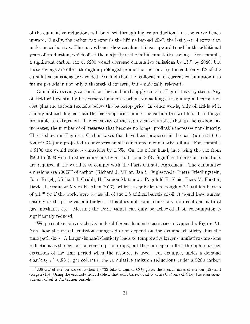
of the umulative redu tions will be o�set through higher produ tion, i.e., the urve bends

upward. Finally, the arbon tax extends the liftime beyond 2097, the last year of extra tion

under no arbon tax. The urves hen e show an almost linear upward trend for the additional

years of produ tion, whi h o�set the majority of the initial umulative savings. For example,

a signi� ant arbon tax of $200 would de rease umulative emissions by 13% by 2080, but

these savings are o�set through a prolonged produ tion period. By the end, only 4% of the

umulative emissions are avoided. We �nd that the reallo ation of urrent onsumption into

future periods in not only a theoreti al on ern, but empiri ally relevant.

Cumulative savings are small as the ombined supply urve in Figure 1 is very steep. Any

oil �eld will eventually be extra ted under a arbon tax as long as the marginal extra tion

ost plus the arbon tax falls below the ba kstop pri e. In other words, only oil �elds with

a marginal ost higher than the ba kstop pri e minus the arbon tax will �nd it no longer

pro�table to extra t oil. The onvexity of the supply urve implies that as the arbon tax

in reases, the number of oil reserves that be ome no longer pro�table in reases non-linearly.

This is shown in Figure 5. Carbon taxes that have been proposed in the past (up to $100 a

ton of CO2) are proje ted to have very small redu tions in umulative oil use. For example,

a $100 tax would redu es emissions by 1.6%. On the other hand, in reasing the tax from

$500 to $600 would redu e emissions by an additional 30%. Signi� ant emission redu tions

are required if the world is to omply with the Paris Climate Agreement. The umulative

emissions are 200GT of arbon (Ri hard J. Millar, Jan S. Fuglestvedt, Pierre Friedlingstein,

Joeri Rogelj, Mi hael J. Grubb, H. Damon Matthews, Ragnhild B. Skeie, Piers M. Forster,

David J. Frame & Myles R. Allen 2017), whi h is equivalent to roughly 2.1 trillion barrels

of oil.

10

So if the world were to use all of the 1.8 trillion barrels of oil, it would have almost

entirely used up the arbon budget. This does not ount emissions from oal and natural

gas, methane, et . Meeting the Paris target an only be a hieved if oil onsumption is

signi� antly redu ed.

We present sensitivity he ks under di�erent demand elasti ities in Appendix Figure A1.

Note how the overall emission hanges do not depend on the demand elasti ity, but the

time path does. A larger demand elasti ity leads to temporarily larger umulative emissions

redu tions as the per-period onsumption drops, but these are again o�set through a further

extension of the time period when the resour e is used. For example, under a demand

elasti ity of -0.86 (right olumn), the umulative emission redu tions under a $200 arbon

10

200 GT of arbon are equivalent to 733 billion tons of CO2 given the atomi mass of arbon (12) and

oxygen (16). Using the estimate from Table 1 that ea h barrel of oil is emits 0.35tons of CO2, the equivalent

amount of oil is 2.1 trillion barrels.

21

tax rea h 20% instead of the 13% in our baseline using an elasti ity of -0.6, but in the end

only 4% less of the oil is onsumed. The demand elasti ity is not not an important driver of

our overall results.

One other important lever that we have held onstant in our analysis so far is the pri e

of the ba kstop R. If this ba kstop pri e be omes lower (e.g., as renewables be ome heaper

and storage be omes available), it would be equivalent to a arbon tax. Re all that �elds

will be extra ted if marginal ost are less than R − τ . In reasing the tax τ or de reasing

R have equivalent e�e ts. Ea h $1 tax per ton of CO2 implies a tax of roughly 35 ents per

barrel, so a redu tion of R = 250 to R = 145 for ∆R = 105 is equivalent to an additional

$300 arbon tax. For example, a $100 arbon tax as well as lowering the ba kstop from

R = 250 to R = 145, would be equivalent to a $400 arbon tax. There are hen e alternative

s enarios that would ombine a arbon tax with investments in alternative energy.

4.2 Welfare E�e ts

We have argued that only a sizable arbon tax, or a arbon tax with advan es in alternative

energy that lower the ost of the ba kstop R have the potential to meaningfully lower oil

onsumption. What are the welfare onsequen es of various taxes? Below, we only ount

the dire t welfare impa ts in the oil market, not ounting the externality redu tion through

limiting greenhouse gas emissions. In prin iple, the arbon tax should be set to equal the

so ial ost of arbon. We are interested in the rami� ations for onsumers and produ ers on

top of that. We highlight that aggregate welfare impa ts are limited even without the bene�t

of CO2 redu tions. Figure 3 has shown that while onsumers initially feel a signi� ant pri e

in rease, over time mu h of the tax is paid by produ ers.

Table 2 presents the net present value of various s enarios. The �rst row states again

the umulative amount of oil that will be extra ted under various arbon taxes. It is simply

the sum of all future extra tion shown in Figure 2. The next three rows present produ er

surplus, onsumer surplus, and tax revenue, all in net present value terms again assuming

a dis ount rate of 3%. Produ er surplus is the di�eren e between the pri e in ea h period

and the extra tion ost as given by Rystad (re all that for undis overed assets these in lude

ost for exploration and development). Our ba kward solution gives us how mu h will be

produ ed by ea h asset on ea h day over the next 100 years as well as the pri e. This allows

us to take the simple di�eren e and dis ount it. Consumer surplus is the area under the

iso-elasti demand urve between the urrent pri e and the ba kstop of R = 250, i.e., the

22

surplus to onsumers from having lower energy pri es than under the ba kstop.

11

We use

quantity and pri e information from Figure 2, al ulate the surplus under the iso-elasti

demand urve, and dis ount it to 2019 with a interest rate of 3%. Finally, tax revenue is the

quantity onsumed times the arbon tax rate.

First, note how for smaller arbon tax rates, e.g., up to $100, the overall welfare impa ts

are limited to at most 1.5%. This is the �ip side of the the fa t that a arbon tax up to

$100 does not signi� ant redu e overall emissions, i.e., there is limited deadweight loss from

taxation (again, not ounting externality redu tions). The roughly equal losses to produ er

and onsumer surplus are o�set by in reased tax revenue. For example, a $100 arbon tax

redu es produ er surplus by 15 trillion, onsumer surplus by 14 trillion, but in reases tax

revenues by 26 trillion, for a net surplus loss of less than 3 trillion.

Se ond, a arbon tax of $500 would redu e arbon emissions by just under 30%, but

expropriate most of the produ ers and onsumer surplus. The reason is that the supply urve

for oil is fairly �at for the �rst two thirds of oil and hen e produ ers �nd it still pro�table to

extra t oil at mu h lower oil pri es. At the same time, onsumer pri es (produ er pri es plus

the tax) in rease enough to also eliminate most of the onsumer surplus. Combined produ er

and onsumer surplus ollapses from 144 trillion to 25 trillion, i.e., by more than 80%. This is

again o�set by 91 trillion in tax revenue. The �at initial supply urve implies that signi� ant

redu tions in oil use are only possible when most of the onsumer and produ er surplus is

wiped out.

We next split the produ er surplus hanges by ountry in Table 3. The redu tion in

produ ers surplus is not proportional but depends on the ost stru ture of ea h ountry. For

example, Saudia Arabia is not only one of the biggest produ ers, but also has really low

produ tion ost, resulting in high produ er surplus. A arbon tax of $200 would eliminate

38% of that surplus. On the other hand, the same arbon tax would eliminate more than 50%

of Canada's surplus, as the ountry extra ts oil from high- ost tar sands, and a omparable

redu tion in pri e hen e implies a large relative redu tion in rents.

Sin e oil demand will likely shift signi� antly between ountries in future years, e.g., a

higher share will be onsumed by developing ountries, an analysis of onsumer surplus by

ountry for all future years is beyond the s ope of this paper as we would have to simulate

the shift in onsumption. Instead we present an analysis for 2016, the last year for whi h

the Energy Information Administration is providing data for most ountries at the time of

writing. Table 4 list the 25 ountries with the highest de rease in overall surplus under a

11

The formula for onsumer surplus for the iso-elasti demand fun tion is

α1+η

[2501+η − p1+η]

23

$50 arbon tax, while Table 5 gives the 25 ountries with the highest gains. All numbers

are in billion dollars. E�e ts on produ er surplus are split into two omponents. Column

(1) gives the revenue e�e t, by multiplying the urrent produ tion of ea h ountry by the

de line in produ er pri e that would result from the $50 arbon tax. The arbon tax will

drive a wedge between produ er and onsumer pri es. While produ er pri es fall, onsumer

pri es in rease and hen e demand will de rease. The drop in demand has to be mat hed by

a drop in produ tion. We present two ounterfa tuals: the �rst shown in olumn (2a) s ales

down the produ tion of ea h ountry by the same relative aggregate drop in produ tion,

eliminating the reserves with the highest marginal ost in ea h ountry. On the other hand,

olumn (2b) eliminates the produ tion of the most expensive reserves around the world.

For example, Saudi Arabia is a low ost produ er and hen e would keep its produ tion

un hanged, while high- ost produ ers like Canada would redu e output by a higher ratio

that the global redu tion in output.

Consumer surplus hanges are given in olumn (3), assuming the same iso-elasti demand

fun tion with an elasti ity of−0.61 in ea h ountry and using 2016 onsumption quantities as

given by EIA. Column (4) is the tax revenue of ea h ountry, assuming that it is proportional

to domesti onsumption after the arbon tax is imposed, i.e., it assumes that ea h ountry

imposes the same arbon tax on onsumption and it is not imposed by produ ing ountries.

Columns (5a) and (5b) give the ombined impa t of produ er surplus, onsumer surplus,

and the tax revenue. The di�eren e between (5a) and (5b) is whether the produ er surplus

omponent (2a) or (2b) are used, respe tively.

Intuitively, the biggest losers in Table 4 are ountries that are net exporters of oil, e.g.,

Saudi Arabia. The drop in produ er surplus is no longer o�set by an in rease in tax revenue,

whi h o urs where oil is onsumed. On the �ip side, winners in Table 5 are generally net

importers of oil, e.g., Japan, China and Germany. The in rease in tax revenue more than

o�sets the de rease in onsumer and produ er surplus.

12

The tables also learly show the

high ost produ ers, e.g., Canada and Brazil. The produ er surplus loss in olumn (2b) is

mu h higher as most of a ountry's reserves should be shut down when the globally most

expensive reserves are used to balan e the implied demand redu tion, while olumn (2a)

redu es ea h ountry's output proportionally. Tables 4 and 5 is to stress that the aggregate

impa ts mask spatial heterogeneity.

12

As previously mentioned, we used onsumption quantity for 2016, the latest year for whi h EIA published

demand estimates around the world at the time of writing. The United States have sin e be ome a net

exporter.

24

4.3 Comparison to Re ent Carbon Taxes

Some regions (e.g., British Columbia) or ountries (Denmark, Finland, Sweden) have estab-

lished arbon taxes. Several studies have argued that these taxes have lead to signi� ant

redu tions in CO2 emissions. For example, Brian Murray & Ni holas Rivers (2015) �nd that

a modest arbon tas of $30 per ton of Co2 has redu ed emissions by 5-15%, while Boqiang

Lin & Xuehui Li (2011) �nd mixed results for S andinavian ountries. Finland seems to

have signi� antly redu ed its emissions, while other ountries do not see signi� ant drop in

emission, likely due to the fa t that some emission intensive se tors are exempt.

These studies only look at partial regulation of small subset of the global e onomy. Their

results are not at odds with ours. A partial regulation of a ountry might indeed redu e

emissions of that ountry as �rms in that ountries shift away from energy as input to

other fa tors or be ome more e� ient. These partial regulation are not expe ted to have a

sizable e�e t on global emissions and have the rami� ation we onsider here: feedba k on

the optimal pri e and extra tion path of an exhaustible resour e. These onsiderations arise

when a global arbon tax were to be imposed. Our study fo uses on su h a global arbon

tax. There is a at h 22: overall emissions are only meaningfully impa ted if all major

emission sour es are regulated, but if we regulate them all, it would have rami� ations on

the extra tion path that we emphasize.

5 Con lusions

In a stati one-period framework a arbon tax is an obvious Pigouvian poli y response to

the global warming problem. However the repla ement of fossil fuels by alternatives will

play out over several de ades, whi h is long enough for intertemporal substitution to ome

into play. This is what is emphasized by the Hotelling model of extra tive resour e markets:

equilibrium is a dynami pro ess not a stati state. As a result, the e�e ts of taxes are not

immediately obvious. Taking the dynami s of resour e use into a ount shows that a arbon

tax may a t in two ways: it an delay the onsumption of a fossil fuel, leading to lower

emissions of greenhouse gases at any date but the same emissions umulatively over time.

Alternatively it may for e a fossil fuel out of the market and so redu e total emissions and

lead to the repla ement of fossil by renewable energy. There are ases in whi h both of these

e�e ts will be seen, in parti ular the ase where there are multiple grades of fossil fuel with

varying extra tion osts. In pra ti e we an expe t to see both e�e ts of a arbon tax, with

the balan e between the two depending on how mu h fossil fuel is selling for a pri e lose to

25

its ba kstop pri e. The latter e�e t is where a arbon tax will redu e fuel onsumption and

greenhouse gas emissions, and seems to be espe ially relevant for the oal and to a lesser

degree natural gas.

Applying our framework to empiri al mi ro-level data on the MECs of rude oil suggests

that a arbon tax would need to be mu h larger than is ommonly suggested to have a

signi� ant impa t on oil onsumption - greater than $100 per ton CO2 - whereas it will

eliminate most oal and mu h gas. A arbon tax of $100 would only redu e umulative oil

emissions by 1.6%. Some of the initial redu tions in oil use are o�set through an extended

time of onsumption. At the same time, global welfare impa ts are limited to a de line of

1.5%. Around 70-80% of the tax will initially be passed on to onsumers, but the passthrough

is de lining in time and even be omes negative in laters years as the tax shifts from the

present to the future. In net present value terms, onsumers and produ ers roughly share

half of the ost of the arbon tax, most of whi h is o�set by arbon tax revenues. Given

the onvexity of the oil supply urve, signi� ant redu tions in oil use an only be a hieved

if most produ er and onsumer surplus are taxed away.

Another important lever is the pri e of the ba kstop R. If this ba kstop pri e be omes

lower (e.g., as renewables be ome heaper and storage be omes available), it would be equiv-

alent to a arbon tax. Re all that �elds will be extra ted if marginal ost are less than R−τ .

In reasing the tax τ or de reasing R have equivalent e�e ts. The result that the marginal

redu tion in oil use is highly onvex in the arbon tax, implies equivalently that a arbon

tax together with a lower ba kstop pri e (e.g., heaper renewables) will de rease arbon

emissions mu h more than either of the two poli y levers by itself.

26

Referen es

Anderson, Soren T., Ryan Kellogg, and Stephen W. Salant. 2018. �Hotelling under

Pressure.� Journal of Politi al E onomy, 126(3): 984�1026.

Asker, John, Allan Collard-Wexler, and Jan De Loe ker. 2019. �(Mis)Allo ation,

Market Power, and Global Oil Extra tion.� Ameri an E onomi Review, 109(4): 1568�

1615.

Cairns, Robert. 2012. �The Green Paradox of the E onomi s of Exhaustible Resour es.�

M Gill University, Department of E onomi s, Working Paper.

Coase, Ronald. 1960. �The Problem of So ial Cost.� Journal of Law and E onomi s, III: 1�

44.

Dasgupta, Partha, and Geo�rey Heal. 1979. E onomi Theory and Exhaustible Re-

sour es. Cambridge Handbooks in E onomi s, Cambridge University Press.

Dasgupta, Parth, Geo�rey Heal, and Joseph Stiglitz. 1980. �The Taxation of Ex-

haustible Resour es.� In Publi Poli y and the Tax System: Essays in Honour of James

Meade. , ed. Gordon Hughes and Geo�rey Heal. Harper Collins.

Gerlagh, Reyer. 2010. �Too Mu h Oil.� Fondazione Eni Enri o Mattei: Nota di Lavoro,

https://www.e onstor.eu/bitstream/10419/43557/1/640265332.pdf.

Hamilton, James D. 2009. �Understanding Crude Oil Pri es.� Energy Journal, 30(2): 179�

206.

Heal, Geo�rey. 1976. �The Relationship between Pri e and Extra tion Cost for a Resour e

with a Ba kstop Te hnology.� Bell Journal of E onomi s, 7(2): 371�378.

Hoel, Mi hael. 2010. �Is There a Green Paradox?� CESifo working Paper 3168,

https://ssrn. om/abstra t=1679663.

Hoel, Mi hael. 2012. �Carbon Taxes and the Green Paradox.� In Climate Change and

Common Sense: Essays in Honour of Tom S helling,. , ed. Robert Hahn and Alistair

Ulph. Oxford University Press.

Hotelling, Harold. 1931. �The E onomi s of Exhaustible Resour es.� Journal of Politi al

E onomy, 39(2): 137�75.

Jensen, Sven, Kristina Mohlin, Karen Pittel, and Thomas Sterner. 2015. �An

Introdu tion to the Green Paradox: The Unintended Consequen es of Climate Poli ies.�

Review of Environmental E onomi s and Poli y, 9(2): 246�265.

Lin, Boqiang, and Xuehui Li. 2011. �The e�e t of arbon tax on per apita CO2 emis-

sions.� Energy Poli y, 39(9): 5137�5146.

27

Millar, Ri hard J., Jan S. Fuglestvedt, Pierre Friedlingstein, Joeri Rogelj,

Mi hael J. Grubb, H. Damon Matthews, Ragnhild B. Skeie, Piers M.

Forster, David J. Frame, and Myles R. Allen. 2017. �Emission budgets and path-

ways onsistent with limiting warming to 1.5C.� Nature Geos ien e, 10: 741�747.

Morris, Adele. n.d.. �The Many Bene�ts of a Carbon Tax.�

Murray, Brian, and Ni holas Rivers. 2015. �British Columbia's revenue-neutral arbon

tax: A review of the latest �grand experiment� in environmental poli y.� Energy Poli y,

86: 674�683.

Pigou, Arthur Ce il. 1920. The E onomi s of Welfare. London:Ma millan.

Sinn, Hans-Werner. 2012. The Green Paradox: A Supply-Side Approa h to Global Warm-

ing. Cambridge, Mass.:M.I.T. Press.

Sinn, Hans-Werner. 2015. �The Green Paradox: A Supply-Side View of the Climate

Problem.� Review of Environmental E onomi s and Poli y, 9(2): 239�245.

van der Ploeg, Ri k, and Cees Withagen. 2010. �Is There Really a Green Paradox?�

CESifo working Paper 2963, https://ssrn. om/abstra t=1562463.

van der Ploeg, Ri k, and Cees Withagen. 2015. �Golbal Warming and the Green

Paradox: A Review of Adverse E�e ts of Climate Poli ies.� Review of Environmental

E onomi s and Poli y, 9(2): 285�303.

28

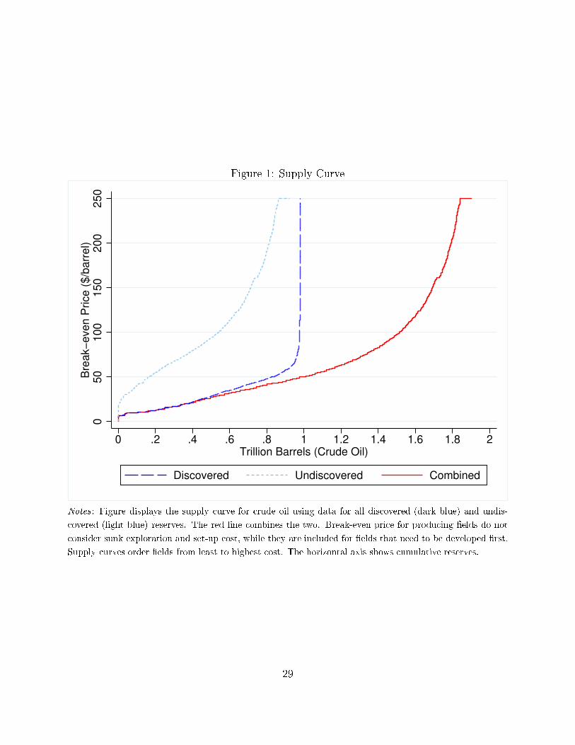
Figure 1: Supply Curve

05

01

00

15

02

00

25

0B

rea

k−

eve

n P

rice

($

/ba

rre

l)

0 .2 .4 .6 .8 1 1.2 1.4 1.6 1.8 2Trillion Barrels (Crude Oil)

Discovered Undiscovered Combined

Notes : Figure displays the supply urve for rude oil using data for all dis overed (dark blue) and undis-

overed (light blue) reserves. The red line ombines the two. Break-even pri e for produ ing �elds do not

onsider sunk exploration and set-up ost, while they are in luded for �elds that need to be developed �rst.

Supply urves order �elds from least to highest ost. The horizontal axis shows umulative reserves.

29

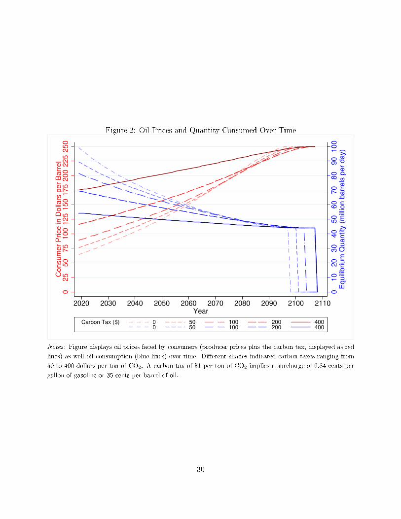
Figure 2: Oil Pri es and Quantity Consumed Over Time

01

02

03

04

05

06

07

08

09

01

00

Eq

uili

briu

m Q

ua

ntity

(m

illio

n b

arr

els

pe

r d

ay)

02

55

07

51

00

12

51

50

17

52

00

22

52

50

Co

nsu

me

r P

rice

in

Do

llars

pe

r B

arr

el

2020 2030 2040 2050 2060 2070 2080 2090 2100 2110Year

Carbon Tax ($) 0 50 100 200 4000 50 100 200 400

Notes : Figure displays oil pri es fa ed by onsumers (produ er pri es plus the arbon tax, displayed as red

lines) as well oil onsumption (blue lines) over time. Di�erent shades indi ated arbon taxes ranging from

50 to 400 dollars per ton of CO2. A arbon tax of $1 per ton of CO2 implies a sur harge of 0.84 ents per

gallon of gasoline or 35 ents per barrel of oil.

30

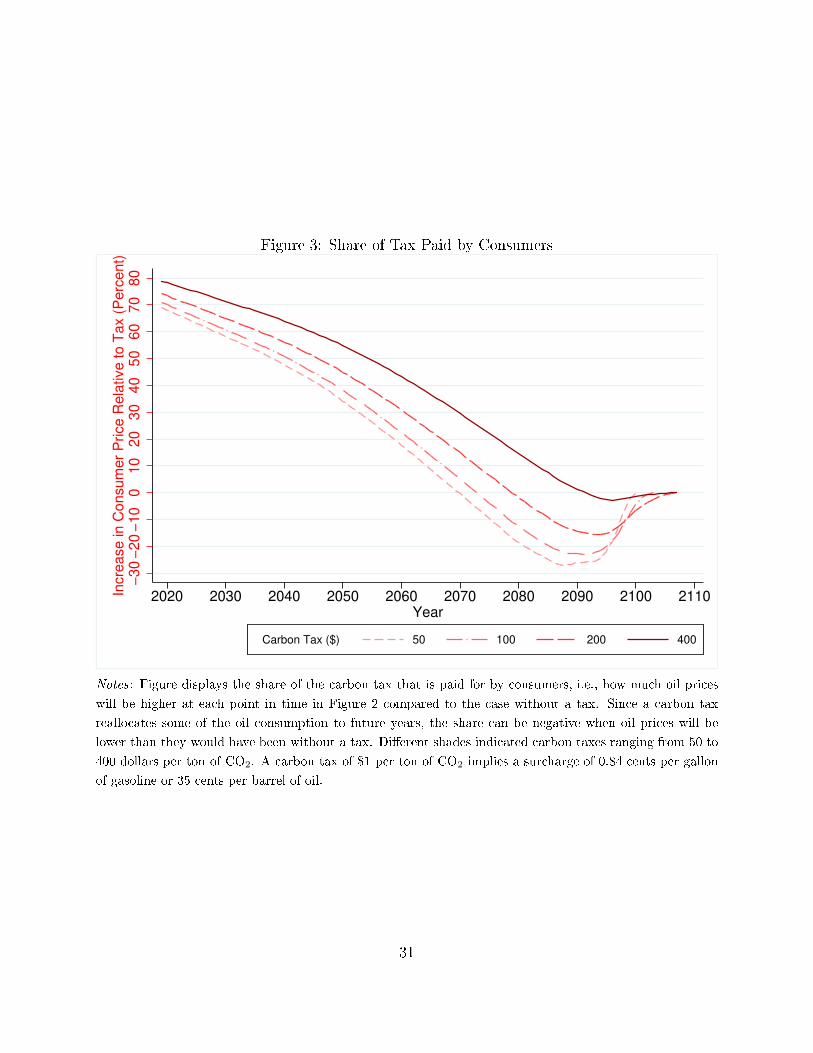
Figure 3: Share of Tax Paid by Consumers

−3

0−

20

−1

00

10

20

30

40

50

60

70

80

Incre

ase

in

Co

nsu

me

r P

rice

Re

lative

to

Ta

x (

Pe

rce

nt)

2020 2030 2040 2050 2060 2070 2080 2090 2100 2110Year

Carbon Tax ($) 50 100 200 400

Notes : Figure displays the share of the arbon tax that is paid for by onsumers, i.e., how mu h oil pri es

will be higher at ea h point in time in Figure 2 ompared to the ase without a tax. Sin e a arbon tax

reallo ates some of the oil onsumption to future years, the share an be negative when oil pri es will be

lower than they would have been without a tax. Di�erent shades indi ated arbon taxes ranging from 50 to

400 dollars per ton of CO2. A arbon tax of $1 per ton of CO2 implies a sur harge of 0.84 ents per gallon

of gasoline or 35 ents per barrel of oil.

31

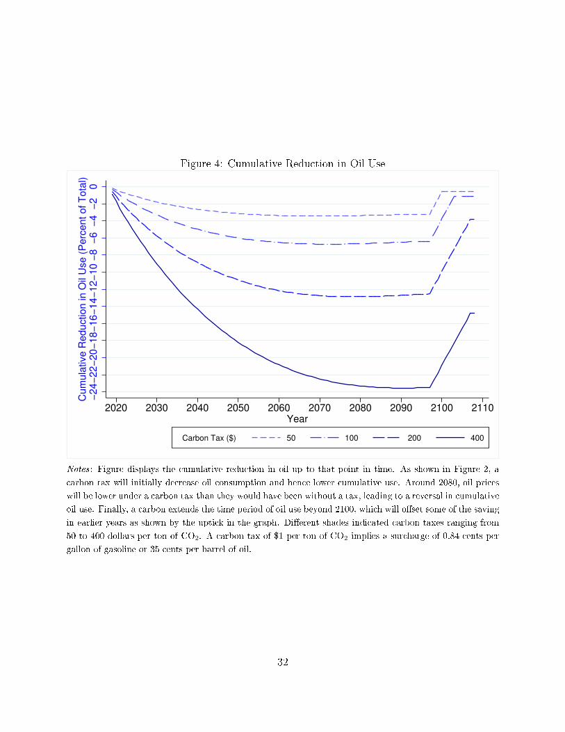
Figure 4: Cumulative Redu tion in Oil Use

−2

4−

22

−2

0−

18

−1

6−

14

−1

2−

10

−8

−6

−4

−2

0C

um

ula

tive

Re

du

ctio

n in

Oil

Use

(P

erc

en

t o

f T

ota

l)

2020 2030 2040 2050 2060 2070 2080 2090 2100 2110Year

Carbon Tax ($) 50 100 200 400

Notes : Figure displays the umulative redu tion in oil up to that point in time. As shown in Figure 2, a

arbon tax will initially de rease oil onsumption and hen e lower umulative use. Around 2080, oil pri es

will be lower under a arbon tax than they would have been without a tax, leading to a reversal in umulative

oil use. Finally, a arbon extends the time period of oil use beyond 2100, whi h will o�set some of the saving

in earlier years as shown by the upti k in the graph. Di�erent shades indi ated arbon taxes ranging from

50 to 400 dollars per ton of CO2. A arbon tax of $1 per ton of CO2 implies a sur harge of 0.84 ents per

gallon of gasoline or 35 ents per barrel of oil.

32

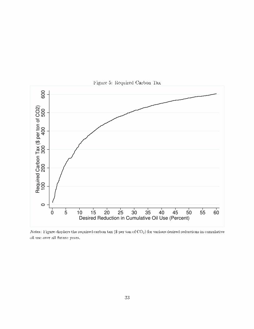
Figure 5: Required Carbon Tax

01

00

20

03

00

40

05

00

60

0R

eq

uire

d C

arb

on

Ta

x (

$ p

er

ton

of

CO

2)

0 5 10 15 20 25 30 35 40 45 50 55 60Desired Reduction in Cumulative Oil Use (Percent)

Notes : Figure displays the required arbon tax ($ per ton of CO2) for various desired redu tions in umulative

oil use over all future years.

33

Table 1: Carbon Tax and Cost of Various Fuels

CO2 Emissions Current Pri e Carbon Tax

Fuel Units (mt per fuel unit) ($ per fuel unit) ($ per fuel unit)

Coal mt 2.86 50 143

Gas mmbtu 0.053 3 2.65

Oil bbl 0.35 60 17.6

Notes : Table translates a uniform arbon tax of $50 per ton into ost for various fuels. The �rst olumn lists

the fuel type, the se ond olumn the ommon unit in whi h the fuel is measured: metri tons (mt), millon

BTU (mmbtu), or barrels (bbl). The third olumn shows the CO2 emissions in metri tons for ea h unit

of a fuel. The fourth olumn gives the urrent average pri e, while the last olumn shows the ost of a $50

arbon tax on ea h unit of fuel.

34

Table 2: Simulated Cumulative E�e ts over all Future Years

Carbon Tax (Dollar per ton of CO2) 0 10 30 50 100 200 400 500 600

Oil Reserves Used (Billion Barrels) 1842 1840 1832 1824 1812 1765 1560 1321 756

Produ er Surplus (Trillion Dollars) 57.36 55.70 52.53 49.53 42.77 31.81 16.89 11.31 5.41

Consumer Surplus (Trillion Dollars) 86.77 85.46 82.80 80.07 73.03 58.29 28.38 14.43 3.35

Tax Revenue (Trillion Dollars) 0.00 2.85 8.39 13.71 26.16 47.78 80.43 91.24 86.32

Total Surplus (Trillion Dollars) 144.13 144.02 143.71 143.32 141.96 137.88 125.71 116.98 95.09

Notes : Table gives the value of all future global oil onsumption, produ er surplus, onsumer surplus and tax revenues. Top header list the

arbon tax, ranging from 10 to 600 dollars per ton of CO2. The �rst row of the Table gives total oil onsumption over all future years. The

remaining rows give the dis ounted net present value using a dis ount rate of 3 per ent. Produ er surplus is the rent (pri e - marginal extra tion

ost), onsumer surplus is the area under the demand urve from the urent pri e to the ba kstop pri e of 250 dollars per barrel. Tax revenue

is the quantity onsumed times the arbon tax.

35

Table 3: Dis ounted Net Produ er Surplus over All Future Years

Carbon Tax 0 10 30 50 100 200 400 500 600

Saudi Arabia 10.06 9.81 9.34 8.90 7.89 6.24 3.92 2.97 1.80

United States 6.56 6.36 5.96 5.59 4.76 3.41 1.61 0.93 0.23

Russia 4.69 4.54 4.27 4.01 3.42 2.48 1.22 0.73 0.21

Iran 3.88 3.78 3.59 3.40 2.99 2.31 1.34 0.96 0.52

Iraq 3.74 3.65 3.48 3.31 2.93 2.32 1.47 1.14 0.72

UAE 2.63 2.57 2.45 2.33 2.08 1.66 1.08 0.84 0.54

China 2.48 2.41 2.27 2.13 1.83 1.34 0.65 0.39 0.12

Canada 2.43 2.35 2.20 2.05 1.73 1.20 0.52 0.27 0.06

Brazil 2.36 2.28 2.13 1.99 1.67 1.15 0.45 0.22 0.05

Kuwait 2.24 2.18 2.08 1.99 1.77 1.41 0.89 0.69 0.44

Venezuela 1.62 1.57 1.46 1.37 1.15 0.80 0.32 0.15 0.02

Mexi o 1.52 1.47 1.39 1.30 1.12 0.81 0.39 0.24 0.09

Kazakhstan 1.42 1.38 1.31 1.24 1.08 0.82 0.45 0.30 0.13

Norway 0.83 0.80 0.76 0.71 0.62 0.45 0.23 0.15 0.06

Australia 0.80 0.78 0.74 0.69 0.60 0.45 0.23 0.14 0.05

Libya 0.71 0.69 0.65 0.62 0.53 0.40 0.21 0.13 0.06

Nigeria 0.69 0.67 0.63 0.59 0.49 0.35 0.14 0.08 0.02

Algeria 0.45 0.43 0.40 0.38 0.32 0.22 0.09 0.05 0.01

India 0.43 0.42 0.40 0.38 0.33 0.25 0.14 0.09 0.04

Azerbaijan 0.42 0.41 0.38 0.36 0.31 0.23 0.12 0.08 0.03

United Kingdom 0.39 0.38 0.36 0.33 0.28 0.21 0.10 0.05 0.01

Somalia 0.36 0.35 0.32 0.30 0.24 0.15 0.03 0.01 0.00

Angola 0.35 0.33 0.31 0.29 0.24 0.16 0.07 0.04 0.01

Indonesia 0.32 0.31 0.29 0.27 0.23 0.16 0.08 0.05 0.02

Argentina 0.31 0.30 0.28 0.26 0.22 0.15 0.06 0.03 0.01

Notes : Table breaks the global produ er surplus of all future oil produ tion (�rst row of Table 2) by ountry

and lists the 25 ountries with the highest surplus under no arbon tax ( olumn 1). Produ er surplus is the

rent (pri e - marginal extra tion ost), dis ounted at 3 per ent dis ount rate and given in trillion 2019 US

dollars. Subsequent olumns give the surplus under various arbon taxes ranging from 10 to 600 dollars per

ton of CO2.

36

Table 4: Change in 2016 Surplus from 50 Dollar Carbon Tax - 25 Biggest Losers

∆ProducerSurplus ∆CS ∆Tax Overall

(1) (2a) (2b) (3) (4) (5a) (5b)

Saudi Arabia -20.61 -19.54 0.00 -13.97 19.10 -35.02 -15.48

Russia -20.00 -18.03 -0.41 -15.36 21.00 -32.38 -14.76

Iraq -8.71 -8.64 -0.04 -3.62 4.96 -16.01 -7.41

Iran -6.88 -6.38 -0.11 -7.63 10.43 -10.46 -4.19

Kuwait -5.49 -5.51 0.00 -1.52 2.08 -10.43 -4.93

UAE -6.05 -5.57 0.00 -3.79 5.18 -10.23 -4.66

Canada -7.08 -3.61 -23.22 -10.45 14.30 -6.85 -26.46

Venezuela -4.04 -3.07 -6.31 -2.53 3.46 -6.18 -9.42

Angola -3.31 -2.31 -2.14 -0.56 0.77 -5.41 -5.24

Norway -3.13 -1.90 -1.80 -0.91 1.25 -4.70 -4.60

Mexi o -4.20 -3.16 -0.81 -8.68 11.87 -4.17 -1.82

Kazakhstan -2.69 -1.92 -1.65 -1.37 1.88 -4.11 -3.84

Nigeria -2.78 -1.54 -1.50 -1.81 2.48 -3.65 -3.62

Algeria -2.11 -1.96 -0.00 -1.81 2.48 -3.40 -1.45

Brazil -4.85 -2.85 -10.82 -12.62 17.26 -3.05 -11.02

Azerbaijan -1.51 -1.23 -0.20 -0.41 0.56 -2.58 -1.55

Oman -1.78 -0.75 -1.06 -0.77 1.06 -2.24 -2.55

Colombia -1.66 -1.08 -3.26 -1.51 2.06 -2.18 -4.36

Qatar -1.27 -1.09 -0.24 -0.73 0.99 -2.09 -1.25

E uador -1.06 -1.01 -0.00 -1.10 1.50 -1.67 -0.66

Libya -0.77 -0.67 0.01 -0.94 1.29 -1.09 -0.42

Congo -0.58 -0.36 -0.36 -0.07 0.10 -0.91 -0.91

Argentina -0.96 -0.83 -0.05 -3.00 4.10 -0.69 0.09

Malaysia -1.12 -0.62 -1.40 -2.99 4.10 -0.64 -1.42

Equatorial Guinea -0.33 -0.22 -2.02 -0.02 0.03 -0.54 -2.34

Notes : Table gives the e�e t of a US$50 arbon tax for the most re ent year in whi h EIA list onsumption

data: 2016. It separates overall surplus hange into hanges in produ er surplus, onsumer surplus, and tax

revenues raised. Column (1) gives the hange in revenue from a pri e de line holding output onstant qi0(pp−

p0). Column (2a) gives the hange in produ er surplus from a onstant proportional hange in quantity

produ ed by all ountries. Columns (2b) repli ate (2a) but no longer require a proportional redu tion in

every ountry but instead retires the �elds with the highest ost in the entire world. Column (3) gives the

hange in onsumer surplus assuming a ommon demand elasti ity of -0.6 using a ountries onsumption

from EIA. Tax revenues are given in olumn (4), whi h are simply the after-tax onsumption times the tax

rate. Overall e�e ts of proportional produ tion adjustments are given in olumns (5a), whi h is the sum of

(1), (2a), (3), and (4). Overall e�e ts when the globally most ostly �elds are retired are given in olumns

(5b), whi h is the sum of (1), (2b), (3), and (4). All numbers are in billion US$.

37

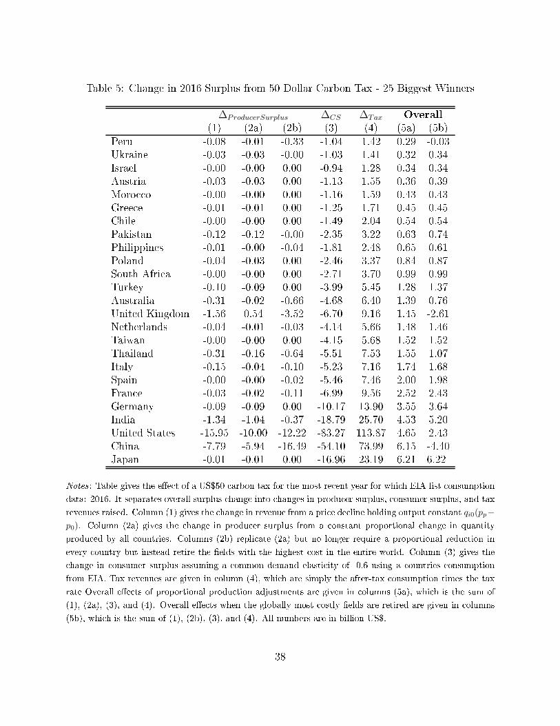
Table 5: Change in 2016 Surplus from 50 Dollar Carbon Tax - 25 Biggest Winners

∆ProducerSurplus ∆CS ∆Tax Overall

(1) (2a) (2b) (3) (4) (5a) (5b)

Peru -0.08 -0.01 -0.33 -1.04 1.42 0.29 -0.03

Ukraine -0.03 -0.03 -0.00 -1.03 1.41 0.32 0.34

Israel -0.00 -0.00 0.00 -0.94 1.28 0.34 0.34

Austria -0.03 -0.03 0.00 -1.13 1.55 0.36 0.39

Moro o -0.00 -0.00 0.00 -1.16 1.59 0.43 0.43

Gree e -0.01 -0.01 0.00 -1.25 1.71 0.45 0.45

Chile -0.00 -0.00 0.00 -1.49 2.04 0.54 0.54

Pakistan -0.12 -0.12 -0.00 -2.35 3.22 0.63 0.74

Philippines -0.01 -0.00 -0.04 -1.81 2.48 0.65 0.61

Poland -0.04 -0.03 0.00 -2.46 3.37 0.84 0.87

South Afri a -0.00 -0.00 0.00 -2.71 3.70 0.99 0.99

Turkey -0.10 -0.09 0.00 -3.99 5.45 1.28 1.37

Australia -0.31 -0.02 -0.66 -4.68 6.40 1.39 0.76

United Kingdom -1.56 0.54 -3.52 -6.70 9.16 1.45 -2.61

Netherlands -0.04 -0.01 -0.03 -4.14 5.66 1.48 1.46

Taiwan -0.00 -0.00 0.00 -4.15 5.68 1.52 1.52

Thailand -0.31 -0.16 -0.64 -5.51 7.53 1.55 1.07

Italy -0.15 -0.04 -0.10 -5.23 7.16 1.74 1.68

Spain -0.00 -0.00 -0.02 -5.46 7.46 2.00 1.98

Fran e -0.03 -0.02 -0.11 -6.99 9.56 2.52 2.43

Germany -0.09 -0.09 0.00 -10.17 13.90 3.55 3.64

India -1.34 -1.04 -0.37 -18.79 25.70 4.53 5.20

United States -15.95 -10.00 -12.22 -83.27 113.87 4.65 2.43

China -7.79 -5.94 -16.49 -54.10 73.99 6.15 -4.40

Japan -0.01 -0.01 0.00 -16.96 23.19 6.21 6.22

Notes : Table gives the e�e t of a US$50 arbon tax for the most re ent year for whi h EIA list onsumption

data: 2016. It separates overall surplus hange into hanges in produ er surplus, onsumer surplus, and tax

revenues raised. Column (1) gives the hange in revenue from a pri e de line holding output onstant qi0(pp−

p0). Column (2a) gives the hange in produ er surplus from a onstant proportional hange in quantity

produ ed by all ountries. Columns (2b) repli ate (2a) but no longer require a proportional redu tion in

every ountry but instead retire the �elds with the highest ost in the entire world. Column (3) gives the

hange in onsumer surplus assuming a ommon demand elasti ity of -0.6 using a ountries onsumption

from EIA. Tax revenues are given in olumn (4), whi h are simply the after-tax onsumption times the tax

rate Overall e�e ts of proportional produ tion adjustments are given in olumns (5a), whi h is the sum of

(1), (2a), (3), and (4). Overall e�e ts when the globally most ostly �elds are retired are given in olumns

(5b), whi h is the sum of (1), (2b), (3), and (4). All numbers are in billion US$.

38

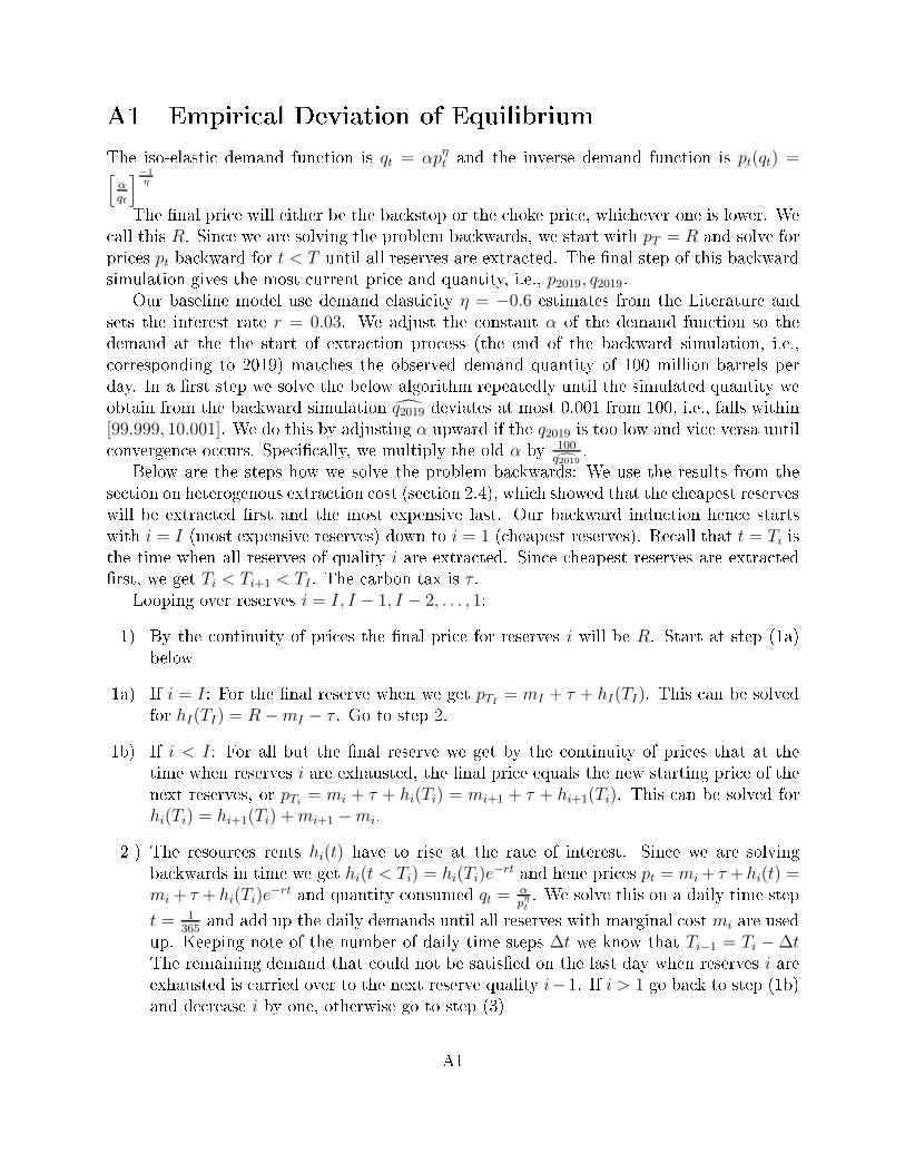
A1 Empiri al Deviation of Equilibrium

The iso-elasti demand fun tion is qt = αpηt and the inverse demand fun tion is pt(qt) =[αqt

]−1

η

The �nal pri e will either be the ba kstop or the hoke pri e, whi hever one is lower. We

all this R. Sin e we are solving the problem ba kwards, we start with pT = R and solve for

pri es pt ba kward for t < T until all reserves are extra ted. The �nal step of this ba kward

simulation gives the most urrent pri e and quantity, i.e., p2019, q2019.Our baseline model use demand elasti ity η = −0.6 estimates from the Literature and

sets the interest rate r = 0.03. We adjust the onstant α of the demand fun tion so the

demand at the the start of extra tion pro ess (the end of the ba kward simulation, i.e.,

orresponding to 2019) mat hes the observed demand quantity of 100 million barrels per

day. In a �rst step we solve the below algorithm repeatedly until the simulated quantity we

obtain from the ba kward simulation q2019 deviates at most 0.001 from 100, i.e., falls within

[99.999, 10.001]. We do this by adjusting α upward if the q2019 is too low and vi e versa until

onvergen e o urs. Spe i� ally, we multiply the old α by

100q2019

.

Below are the steps how we solve the problem ba kwards: We use the results from the

se tion on heterogenous extra tion ost (se tion 2.4), whi h showed that the heapest reserves

will be extra ted �rst and the most expensive last. Our ba kward indu tion hen e starts

with i = I (most expensive reserves) down to i = 1 ( heapest reserves). Re all that t = Ti is

the time when all reserves of quality i are extra ted. Sin e heapest reserves are extra ted�rst, we get Ti < Ti+1 < TI . The arbon tax is τ .

Looping over reserves i = I, I − 1, I − 2, . . . , 1:

1) By the ontinuity of pri es the �nal pri e for reserves i will be R. Start at step (1a)

below

1a) If i = I: For the �nal reserve when we get pTI= mI + τ + hI(TI). This an be solved

for hI(TI) = R−mI − τ . Go to step 2.

1b) If i < I: For all but the �nal reserve we get by the ontinuity of pri es that at the

time when reserves i are exhausted, the �nal pri e equals the new starting pri e of the

next reserves, or pTi= mi + τ + hi(Ti) = mi+1 + τ + hi+1(Ti). This an be solved for

hi(Ti) = hi+1(Ti) +mi+1 −mi.

2 ) The resour es rents hi(t) have to rise at the rate of interest. Sin e we are solving

ba kwards in time we get hi(t < Ti) = hi(Ti)e−rt

and hene pri es pt = mi+ τ +hi(t) =mi + τ + hi(Ti)e

−rtand quantity onsumed qt =

αpηt. We solve this on a daily time step

t = 1365

and add up the daily demands until all reserves with marginal ost mi are used

up. Keeping note of the number of daily time steps ∆t we know that Ti−1 = Ti −∆tThe remaining demand that ould not be satis�ed on the last day when reserves i areexhausted is arried over to the next reserve quality i−1. If i > 1 go ba k to step (1b)

and de rease i by one, otherwise go to step (3)

A1

3) This gives us the extra tion time for reserves i = 1 . . . I and TI . We renormalize time

so that the urrent pri e / onsumption are labeled p2019, q2019

A2

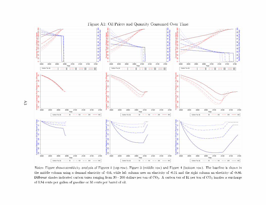
Figure A1: Oil Pri es and Quantity Consumed Over Time

01

02

03

04

05

06

07

08

09

01

00

Eq

uili

briu

m Q

ua

ntity

(m

illio

n b

arr

els

pe

r d

ay)

02

55

07

51

00

12

51

50

17

52

00

22

52

50

Co

nsu

me

r P

rice

in

Do

llars

pe

r B

arr

el

2020 2040 2060 2080 2100 2120 2140 2160Year

Carbon Tax ($) 0 50 100 200 4000 50 100 200 400

01

02

03

04

05

06

07

08

09

01

00

Eq

uili

briu

m Q

ua

ntity

(m

illio

n b

arr

els

pe

r d

ay)

02

55

07

51

00

12

51

50

17

52

00

22

52

50

Co

nsu

me

r P

rice

in

Do

llars

pe

r B

arr

el

2020 2040 2060 2080 2100 2120 2140 2160Year

Carbon Tax ($) 0 50 100 200 4000 50 100 200 400

01

02

03

04

05

06

07

08

09

01

00

Eq

uili

briu

m Q

ua

ntity

(m

illio

n b

arr

els

pe

r d

ay)

02

55

07

51

00

12

51

50

17

52

00

22

52

50

Co

nsu

me

r P

rice

in

Do

llars

pe

r B

arr

el

2020 2040 2060 2080 2100 2120 2140 2160Year

Carbon Tax ($) 0 50 100 200 4000 50 100 200 400

−7

5−

50

−2

50

25

50

75

Incre

ase

in

Co

nsu

me

r P

rice

Re

lative

to

Ta

x (

Pe

rce

nt)

2020 2040 2060 2080 2100 2120 2140 2160Year

Carbon Tax ($) 50 100 200 400

−7

5−

50

−2

50

25

50

75

Incre

ase

in

Co

nsu

me

r P

rice

Re

lative

to

Ta

x (

Pe

rce

nt)

2020 2040 2060 2080 2100 2120 2140 2160Year

Carbon Tax ($) 50 100 200 400

−7

5−

50

−2

50

25

50

75

Incre

ase

in

Co

nsu

me

r P

rice

Re

lative

to

Ta

x (

Pe

rce

nt)

2020 2040 2060 2080 2100 2120 2140 2160Year

Carbon Tax ($) 50 100 200 400

−3

5−

30

−2

5−

20

−1

5−

10

−5

0C

um

ula

tive

Re

du

ctio

n in

Oil

Use

(P

erc

en

t o

f T

ota

l)

2020 2040 2060 2080 2100 2120 2140 2160Year

Carbon Tax ($) 50 100 200 400

−3

5−

30

−2

5−

20

−1

5−

10

−5

0C

um

ula

tive

Re

du

ctio

n in

Oil

Use

(P

erc

en

t o

f T

ota

l)

2020 2040 2060 2080 2100 2120 2140 2160Year

Carbon Tax ($) 50 100 200 400

−3

5−

30

−2

5−

20

−1

5−

10

−5

0C

um

ula

tive

Re

du

ctio

n in

Oil

Use

(P

erc

en

t o

f T

ota

l)

2020 2040 2060 2080 2100 2120 2140 2160Year

Carbon Tax ($) 50 100 200 400

Notes : Figure shows sensitivity analysis of Figures 2 (top row), Figure 3 (middle row) and Figure 4 (bottom row). The baseline is shown in

the middle olumn using a demand elasti ity of -0.6, while left olumn uses an elasti ity of -0.21 and the right olumn an elasti ity of -0.86.

Di�erent shades indi ated arbon taxes ranging from 30 - 200 dollars per ton of CO2. A arbon tax of $1 per ton of CO2 implies a sur harge

of 0.84 ents per gallon of gasoline or 35 ents per barrel of oil.

A3