Embed Size (px)
Citation preview
PAPER MONEY
CHRISTOPHER A. SIMS
ABSTRACT. Drastic changes in central bank operations and monetary institutions in
recent years have made previously standard approaches to explaining the determina-
tion of the price level obsolete. Recent expansions of central bank balance sheets and
of the levels of rich-country sovereign debt, as well as the evolving political economy
of the European Monetary Union, have made it clear that fiscal policy and monetary
policy are intertwined. Our thinking and teaching about inflation, monetary policy
and fiscal policy should be based on models that recognize fiscal-monetary policy
interactions.
I. INTRODUCTION
Central banks since 2008 in many countries have greatly expanded their balance
sheets, rapidly creating large amounts of what used to be called “high powered
money”, without creating inflation. The European Central Bank’s policies and pro-
posals for Europe-wide bank supervision are at the center of hot disputes because
of their fiscal policy implications. The US and Japan are accumulating debt at rates
that are unprecedented in peacetime, which some worry may eventually generate
Date: February 7, 2013.
c⃝2013 by Christopher A. Sims. This document is licensed under the Creative Commons
Attribution-NonCommercial-ShareAlike 3.0 Unported License. http://creativecommons.org/
licenses/by-nc-sa/3.0/.1
PAPER MONEY 2
inflation. Most central banks now pay interest on reserve deposits, making those de-
posits part of the government’s interest-bearing debt. These developments make it
clear that monetary and fiscal policy are tied together, and that conventional macro
models with non-interest-bearing high-powered money, a “money multiplier”, and
a tight relation between the price level and the quantity of “money” are inadequate
as a framework for current policy discussions.
The literature on the fiscal theory of the price level, or FTPL, integrates discus-
sion of monetary and fiscal policy, recognizing that fiscal policy can be a determi-
nant, or even the sole determinant, of the price level.1 The first papers in the area
may have seemed technical — they showed that when the government budget con-
straint is properly taken into account, conditions for existence and uniqueness of the
price level in dynamic general equilibrium were different from what they seemed in
conventional models. They may also have seemed esoteric — they questioned con-
ventional analysis most strongly in policy configurations that in the 1990’s seemed
unlike any observed in rich economies in recent history.2
This paper tries to bring FTPL down to earth. It begins by citing some results from
FTPL analysis and showing how they apply to current policy discussions. It then
presents a couple of simple models illustrating FTPL, using them to make clear how1Many of the insights of the FTPL literature are implicit in Neil Wallace’s earlier paper (1981).
Wallace presented a model in which conventional monetary policy actions had no effect on the price
level so long as fiscal policy were held constant. Of course this implied that in his model fiscal policy
determined the price level, though Wallace did not put it that way.2Some of the important papers in this area are Leeper (1991), Woodford (1995), Cochrane (1998),
and Davig and Leeper (2006).
PAPER MONEY 3
the results used earlier in the paper arise and to refute some of the objections to and
fallacies concerning FTPL that still circulate among economists.
II. INSIGHTS FROM FTPL, AND THEIR APPLICATION
II.1. Monetary policy actions, to be effective, must induce a fiscal policy response.
This is easiest to understand in high-inflation, high nominal debt, economies where
fiscal policy is frozen by political deadlock or chicanery. In such an economy, the
interest rate will be high, and with a high level of debt, the interest expense com-
ponent of the budget is substantial, possibly even dominant. If inflation rises still
higher, the usual monetary policy prescription would be for the policy interest rate
to increase, by even more than the rise in the inflation rate.3 But if the legislature
in such an economy is gridlocked, the central bank may realize that an interest rate
increase will pass right through the government budget, with an increased rate of
issue of nominal debt the only fiscal effect of the interest rate rise. If this is indeed
the situation, and private sector bond buyers understand the situation, the interest
rate rise will have no contractionary effect. Indeed, it will increase the rate of infla-
tion rather than decrease it. The central bank, understanding this, may then forgo
following the conventional policy prescription. In doing so it is not accelerating the
inflation, it is damping it.4
3This is sometimes called the “Taylor principle”, that monetary policy should respond to inflation
changes strongly enough to raise real rates when inflation increases and lower them when inflation
decreases.
4Loyo (2000) discusses a period in Brazil where this analysis applies.

PAPER MONEY 4
In the 1990’s this may have seemed an analysis that applied at most to some mis-
managed Latin American economies, but consider the reasoning many economists
(including me) have used to argue that the great expansion of the balance sheet of
the US Federal Reserve system in the last four years need not generate inflationary
pressure. The Fed now has the authority to pay interest on reserve balances. While
the rates are now low (though still in excess of rates on short term US Treasury Bills),
the Fed is free to raise them if inflationary pressures arise. Even if it undertakes
no open market operations to change the amount of reserves, raising the rates on
reserves would have a powerful contractionary effect. Banks would have little in-
centive to expand their lending if perfectly safe reserve deposits paid interest at a
rate comparable to loan rates.
But this story, like any story about the effects of monetary policy, has a fiscal pol-
icy back story. Because reserve deposits and Treasury securities are close substitutes,
raising the rate on reserve deposits would also raise rates on government debt gen-
erally. The level of US government debt relative to GDP is at unprecedented levels.
If debt were at 100% of GDP, a rise in interest rates to 6% from its current level of
about 2% would bring interest expense, now less than 10% of total Federal govern-
ment expenditure, to 30% of government expenditure, increasing the conventionally
measured deficit drastically if there were no response of fiscal policy. Would there
be a response? Some years ago the answer might have been, “Surely yes”. But the
increase in the conventional deficit would be so large that the response would have
to involve substantial increases in tax revenue. With recent repeated Congressional
PAPER MONEY 5
games of chicken over the debt limit and inability to bargain to a resolution of long-
term budget problems, the answer may now be in some doubt.
With the central bank keeping interest rates stable in the face of inflation fluctua-
tions and fiscal authorities not increasing primary surpluses in response to increased
real debt, the price level is still likely to be determinate. But the main determinant of
inflation becomes the fiscal deficit, rather than changes in the usual instruments of
monetary policy.
II.2. Paper money requires fiscal backing. It is easy to construct models of economies
in which unbacked paper money can have value, but in such models it is gener-
ally also possible for money to be valueless, or to dwindle rapidly in value so that
the economy approaches a barter equilibrium. In such models, introducing taxa-
tion either to pay interest on government liabilities or to contract the supply of non-
interest-bearing liabilities (and thus, via deflation, create a real return) tends to re-
solve the indeterminacy and provide a uniquely determined price level. The first
two examples in section III below show quite different models in which this pattern
of results hold.
Depending on the institutional setup, the fiscal backing can be apparent in equi-
librium, as with taxation to service a stable volume of nominal debt, or it can be
implicit, invoked only under unusual circumstances, as with a commitment to trea-
sury transfers to the central bank if the central bank balance sheet deteriorates. But
in evaluating monetary and fiscal institutions, the question of the nature of fiscal
backing for the price level is a useful starting point. It led me (2004; 1999) to think
PAPER MONEY 6
about where fiscal backing could come from in the EMU and what kinds of condi-
tions might force the EMU to confront the need for fiscal backing. Those two papers
speculated about policy dilemmas that at the time might have been seen as obscure
and unlikely, but now seem practically relevant. The policy discussion in the EMU
during this recent crisis period has focused on fiscal transfers that will arise as par-
tial default on Greek and possibly other Euro area sovereign debt occurs. While
resolving the allocation of these losses that have already occurred is important, con-
troversy over them has hindered discussion of ways to provide clear fiscal backing
for the Euro, which is in many ways an easier problem. I discuss these issues in more
detail in Sims (2012).
II.3. Central bank balance sheets matter, because they connect monetary and fiscal
policy. Formerly, there were monetary economists who argued that the central bank
balance sheet is an accounting fiction, of no substantive interest. It is true that the
implications of having negative net worth at current market values are different for
a central bank and an ordinary firm or private bank. A firm with negative net worth
is likely to find its creditors demanding payment, and is unlikely to be able to pay
them all. A central bank can “print money” — offer deposits as payment for its
bills. It will not be subject to the usual sort of run, then, in which creditors fear not
being paid and hence demand immediate payment. Its liabilities are denominated
in government paper, which it can produce at will.
PAPER MONEY 7
On top of this, most economists have thought of central banks as part of the gov-
ernment, with the only balance sheet that really matters being that of the government
as a whole.
But both of these arguments come apart when the central bank aims at control-
ling the price level and fiscal and monetary policy are not set jointly. Traditional
contractionary open market operations require selling assets to shrink the amount
of reserve deposits and currency. If the central bank is in the red, an aggressively
contractionary policy may not be possible, because people will see that it would
require selling more assets than the central bank actually has.5 If the negative-net-
worth central bank tries to contract by raising interest rates on reserves, yet wants
to avoid expanding reserves, it is likely to need to sell assets to finance the interest
on reserves, again putting it on an unsustainable path. Of course, if the treasury
stands ready to back up the central bank — providing additional assets to the cen-
tral bank in the form of interest-bearing securities whenever necessary — then the
central bank balance sheet is indeed irrelevant.
In thinking about central bank policy when fiscal backing from the treasury is ab-
sent or uncertain, it helps to consider what “fiscal backing” the central bank can pro-
vide on its own, without assistance from the treasury. Of course central banks cannot
impose explicit taxes, but they do have access to an implicit tax: seignorage. Even if
its balance sheet shows negative net worth at current market values, a central bank
can maintain a uniquely determined price level by using its seignorage revenues to
5Sims (2005) showed that this insight generalizes to Taylor rules, where negative net worth puts an
upper bound on the coefficient on inflation in the monetary policy rule.
PAPER MONEY 8
restore its balance sheet. But seignorage revenue depends on the inflation rate, gen-
erally increasing with the rate of inflation except at extremely high inflation rates. A
central bank with a severely enough impaired balance sheet may not be able to pin
down the price level without treasury assistance, but modestly negative net worth
can generally be “worked off” by seignorage. Of course most central banks see their
task as maintaining low inflation, so balance sheet problems, by requiring inflation
to generate seignorage, can be an obstacle to the central bank’s achieving its policy
objectives. Even a central bank with positive net worth may be inhibited in taking
some policy actions by fear of the consequences of negative net worth. Lender of
last resort operations, for example, even when they have positive expected return,
generally pose some risk of losses. A central bank with uncertain fiscal backing may
hesitate to undertake such operations out of fear of their balance sheet consequences.
A simple model of balance sheet dynamics for a central bank with negative net
worth and no fiscal backing appears in my earlier paper Sims (2005). However that
paper assumes the central bank has non-interest-bearing liabilities and short-term
treasury bonds as assets. The US Federal Reserve system pays interest on its reserve
liabilities and holds substantial amounts of long-maturity debt. It has been argued
(by me, among others) that the Fed can take contractionary action by raising the rate
paid on reserves, without necessarily selling its assets. But this argument assumes
fiscal backing. Without it, high interest on reserves, while interest on long-maturity
debt remains low, can create negative seignorage, even in the presence of inflation.

PAPER MONEY 9
In the US and the Euro area today, it is not certain that fiscal repair of central bank
balance sheets would emerge. In the Euro area, there is a formal “capital key”, spec-
ifying in what proportions governments in the EMU should provide capital when
the ECB calls for a capital infusion. But if the capital called for were substantial, and
the call came in the wake of ECB policy actions that were politically unpopular in
some countries, the provision of capital might not be automatic. Perhaps equally
important is that, foreseeing the risk of a capital call and its implicit fiscal transfers,
the ECB’s governing board might refuse to authorize market-stabilizing actions by
the ECB that an ordinary central bank would have undertaken.
In the US, the risk is that the need for capital infusion would most likely arise
in the wake of stringent monetary policy tightening that caused capital losses on the
Fed’s long term debt holdings and required an increased stream of interest payments
on reserves. These actions would be restraining growth and forcing Congress to con-
front increased deficits arising from increased interest expense. In an environment
where Congress cannot agree to let the debt limit increase to accommodate its own
spending and revenue legislation, it is not hard to imagine Congress blaming the Fed
for the painful decisions it faces and in the process casting doubt on its commitment
to recapitalize the Fed.
II.4. Nominal debt and real debt are very different. Real sovereign debt promises
future payments of something the government may not have available — gold, un-
der the gold standard, Euros for individual country members of the EMU, dollars
PAPER MONEY 10
for developing countries that borrow mainly in foreign currency. Nominal sover-
eign debt promises only future payments of government paper, which is always
available. Both types of debt must satisfy the equilibrium condition that the real
value of the country’s debt is the discounted present value of future primary sur-
pluses — revenues in excess of expenditures other than interest payments. But if
an adverse fiscal development increases debt, the increased real debt will require
increased future primary surpluses, whereas with nominal debt there are two other
ways to restore balance — inflation, which directly reduces the real value of future
commitments, and changes in the nominal interest rate, which will change the cur-
rent market value of long term debt.
Obviously outright default on nominal debt is much less likely than default on
real debt. So long as the country is capable of generating any positive stream of
primary surpluses, its debt will have non-zero real value. But if debt is real and the
country finds itself unable to maintain primary surpluses above its predetermined
real debt service commitment, it must default, even if in absolute terms it is running
substantial primary surpluses.
II.4.1. Nominal debt is a cushion, like equity. In a deterministic steady state, investors
will insist on nominal interest rates high enough to compensate for inflation’s effect
on the real value of their debt holdings. Real returns on government debt will be the
same whether it is nominal or real. But if nominal interest rates fall after the date of
issue of long-term nominal debt with a fixed coupon rate, the market value of the
PAPER MONEY 11
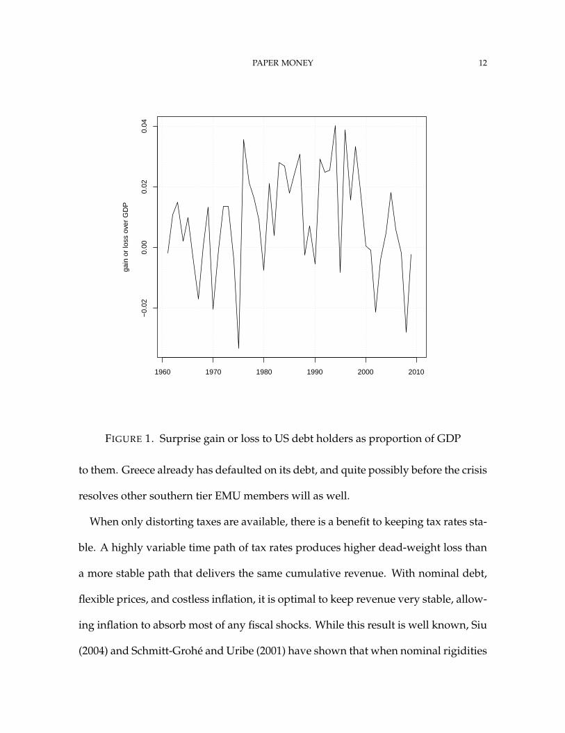
debt will rise, providing the debt holder with an unanticipated higher return. If in-
flation occurs at a higher than expected rate, the real value of nominal debt, whatever
its maturity, suffers an unanticipated decline. These mechanisms can cushion the im-
pact of unexpected changes in the fiscal situation. We live in a stochastic world, and
surprises in returns on government debt from these two mechanisms are substantial.
Figure 1 shows a time series of surprise gains and losses on US government debt as
a fraction of GDP.6 The surprise gains and losses relative to GDP have been of the
same order of magnitude as year to year fluctuations in the fiscal deficit. Were they
displayed as fractions of the value of outstanding debt, so they became surprises in
rates of return, they would be much larger. It is clearly not a good approximation to
model the US economy as if debt were real, even though a considerable part of the
literature on optimal fiscal policy does so.
The southern countries in the Euro area are now reckoning with the consequences
of their having, by joining the Euro, made their sovereign debt real. The 2008-9 crisis
led to great expansion of their debts, and the nominal debt cushion is not available
6The order of magnitude of the surprise gains and losses in the chart is robust to various ways of
computing them, but the time path itself is not. Different ways of computing expected inflation and
one-year returns on long debt change the results. The results in the chart treat the Federal Reserve
system as outside the government, so its gains and losses are included. Since 2009, with the Fed’s
expanded balance sheet and interest being paid on reserves, treatment of it as inside or outside the
government matters a great deal, and proper treatment of its interest-bearing reserve liabilities is a
challenge. See the data appendix.
PAPER MONEY 12
gain
or
loss
ove
r G
DP
1960 1970 1980 1990 2000 2010
−0.
020.
000.
020.
04
FIGURE 1. Surprise gain or loss to US debt holders as proportion of GDP
to them. Greece already has defaulted on its debt, and quite possibly before the crisis
resolves other southern tier EMU members will as well.
When only distorting taxes are available, there is a benefit to keeping tax rates sta-
ble. A highly variable time path of tax rates produces higher dead-weight loss than
a more stable path that delivers the same cumulative revenue. With nominal debt,
flexible prices, and costless inflation, it is optimal to keep revenue very stable, allow-
ing inflation to absorb most of any fiscal shocks. While this result is well known, Siu
(2004) and Schmitt-Grohé and Uribe (2001) have shown that when nominal rigidities
PAPER MONEY 13
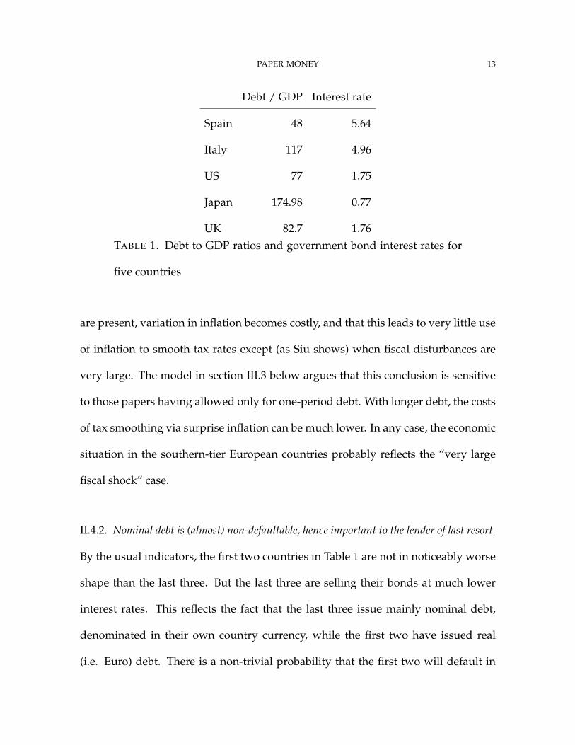
Debt / GDP Interest rate
Spain 48 5.64
Italy 117 4.96
US 77 1.75
Japan 174.98 0.77
UK 82.7 1.76TABLE 1. Debt to GDP ratios and government bond interest rates for
five countries
are present, variation in inflation becomes costly, and that this leads to very little use
of inflation to smooth tax rates except (as Siu shows) when fiscal disturbances are
very large. The model in section III.3 below argues that this conclusion is sensitive
to those papers having allowed only for one-period debt. With longer debt, the costs
of tax smoothing via surprise inflation can be much lower. In any case, the economic
situation in the southern-tier European countries probably reflects the “very large
fiscal shock” case.
II.4.2. Nominal debt is (almost) non-defaultable, hence important to the lender of last resort.
By the usual indicators, the first two countries in Table 1 are not in noticeably worse
shape than the last three. But the last three are selling their bonds at much lower
interest rates. This reflects the fact that the last three issue mainly nominal debt,
denominated in their own country currency, while the first two have issued real
(i.e. Euro) debt. There is a non-trivial probability that the first two will default in
PAPER MONEY 14
some form, while the latter three are quite unlikely to default, because their debt is
nominal.
Economists and journalists sometimes treat inflation as a form of default, but it is
not. Default is a situation where the contracted payments cannot be delivered, and
the contract does not specify what happens in that eventuality. For private firms, this
leads to renegotiation and/or court proceedings. There can be a long period in which
investors cannot get access to their investments and the amount that will be returned
to them remains unknown. Creditors holding different maturities or types of debt
may suffer different degrees of loss, and the allocation of losses across creditors may
be uncertain. For example, a minor default may involve a modest delay in returning
principal of a short term debt. Other creditors may be unaffected, or, if the holder of
the short debt goes to court, all debtors may find themselves impaired. Similar, or
perhaps more severe, uncertainties surround sovereign default.
Unanticipated high inflation does impose losses on investors in nominal sover-
eign debt, but it does not involve renegotiation or court proceedings. Contracted
payments are made. The securities remain tradable. In the same state of uncertainty
about future primary surpluses, therefore, investors are likely to be much more un-
certain about the return on their own investment in sovereign debt when resolution
of the fiscal imbalance has to come from default, rather than inflation and nominal
interest rate changes.
In a financial panic, counterparty risk becomes pervasive among market partici-
pants and credit markets freeze up. An institution of unquestioned soundness and
PAPER MONEY 15
liquidity can remedy the situation by lending freely. While large private banks can
and have historically sometimes acted as such a lender of last resort, any private in-
stitution that attempts it risks itself becoming subject to worries about liquidity. A
central bank, backed by a treasury that can run primary surpluses and issue nomi-
nal debt, is an ideal lender of last resort. Because it can create reserve money, it need
never default. If it takes capital losses, and it is not backed by a fiscal authority, it
could be forced to run a high inflation to restore its balance sheet, but this will not be
a problem if it has fiscal backing. Europe, in setting up its Monetary Union, did not
contemplate the ECB’s taking on a lender of last resort role. Individual country cen-
tral banks can no longer play the role, because they have no independent authority
to create reserve money and their country treasuries issue only real debt. During the
recent crisis the ECB has in fact played a lender of last resort role, though its effec-
tiveness is limited because its actions and announcements in this role are regularly
criticized by some northern-tier economic officials.
III. MODELS
III.1. Samuelson’s pure consumption loan model, with storage. This model is one
where, without tax backing for debt or money, the price level is indeterminate. The
model in that case has one stable price level, in which the real allocation is efficient,
and a continuum of other possible initial price levels, each of which corresponds
to an inefficient equilibrium in which the real value of government debt or money
shrinks toward zero. If the government runs a primary surplus (revenues in excess
of non-interest expenditures), private agents see the future taxes as reducing their
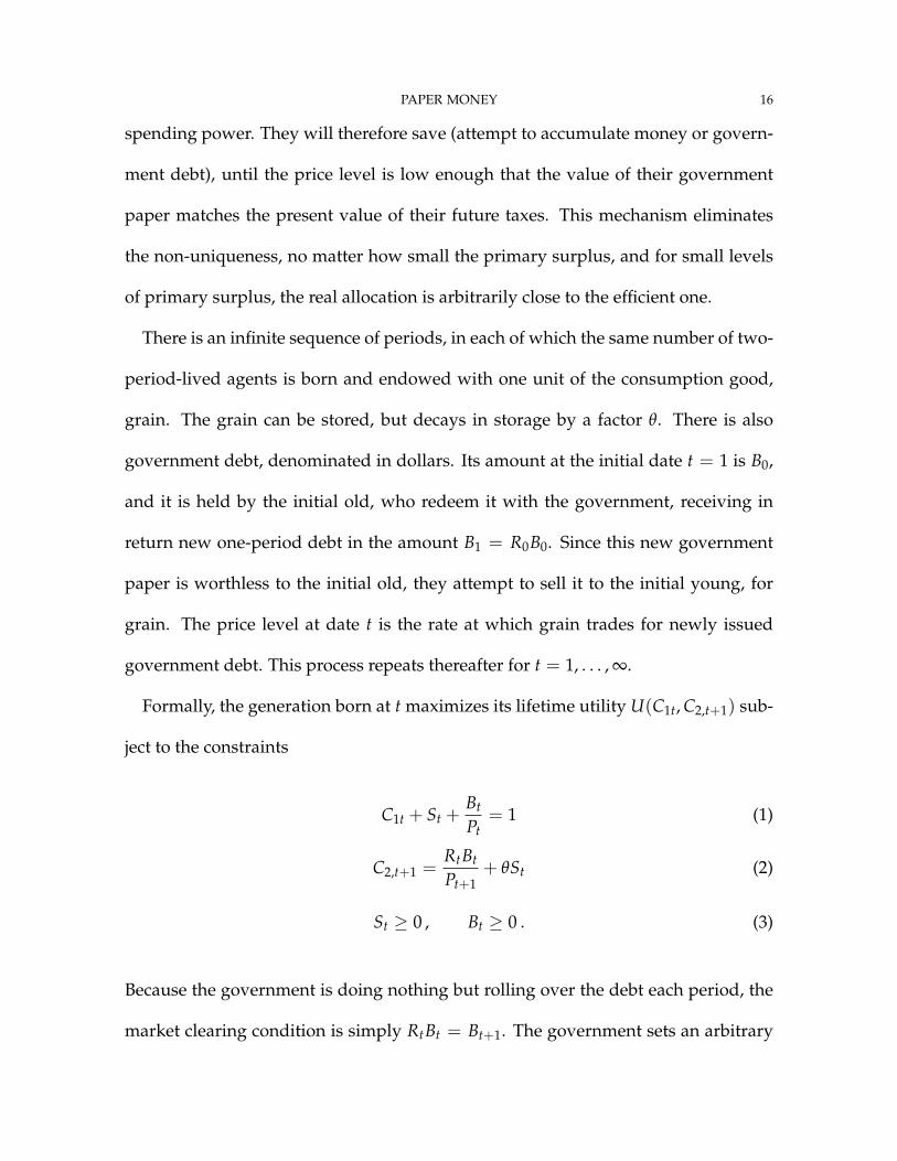
PAPER MONEY 16
spending power. They will therefore save (attempt to accumulate money or govern-
ment debt), until the price level is low enough that the value of their government
paper matches the present value of their future taxes. This mechanism eliminates
the non-uniqueness, no matter how small the primary surplus, and for small levels
of primary surplus, the real allocation is arbitrarily close to the efficient one.
There is an infinite sequence of periods, in each of which the same number of two-
period-lived agents is born and endowed with one unit of the consumption good,
grain. The grain can be stored, but decays in storage by a factor θ. There is also
government debt, denominated in dollars. Its amount at the initial date t = 1 is B0,
and it is held by the initial old, who redeem it with the government, receiving in
return new one-period debt in the amount B1 = R0B0. Since this new government
paper is worthless to the initial old, they attempt to sell it to the initial young, for
grain. The price level at date t is the rate at which grain trades for newly issued
government debt. This process repeats thereafter for t = 1, . . . , ∞.
Formally, the generation born at t maximizes its lifetime utility U(C1t, C2,t+1) sub-
ject to the constraints
C1t + St +Bt
Pt= 1 (1)
C2,t+1 =RtBt
Pt+1+ θSt (2)
St ≥ 0 , Bt ≥ 0 . (3)
Because the government is doing nothing but rolling over the debt each period, the
market clearing condition is simply RtBt = Bt+1. The government sets an arbitrary
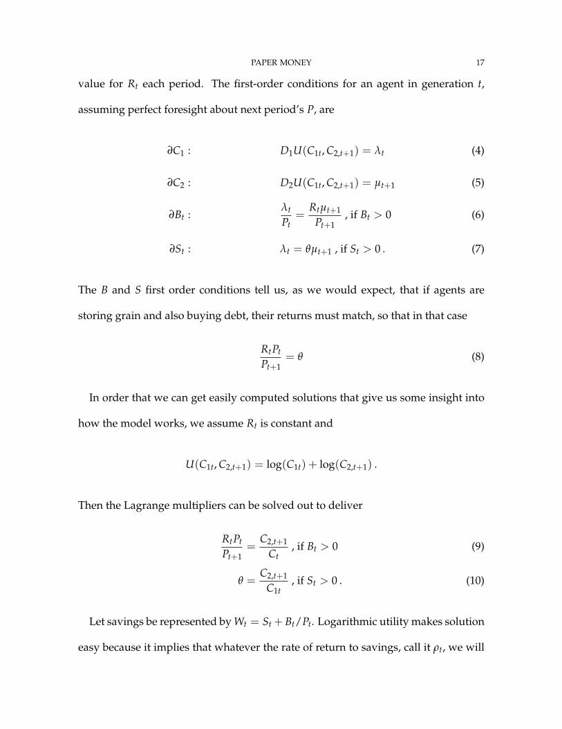
PAPER MONEY 17
value for Rt each period. The first-order conditions for an agent in generation t,
assuming perfect foresight about next period’s P, are
∂C1 : D1U(C1t, C2,t+1) = λt (4)
∂C2 : D2U(C1t, C2,t+1) = µt+1 (5)
∂Bt :λt
Pt=
Rtµt+1
Pt+1, if Bt > 0 (6)
∂St : λt = θµt+1 , if St > 0 . (7)
The B and S first order conditions tell us, as we would expect, that if agents are
storing grain and also buying debt, their returns must match, so that in that case
RtPt
Pt+1= θ (8)
In order that we can get easily computed solutions that give us some insight into
how the model works, we assume Rt is constant and
U(C1t, C2,t+1) = log(C1t) + log(C2,t+1) .
Then the Lagrange multipliers can be solved out to deliver
RtPt
Pt+1=
C2,t+1
Ct, if Bt > 0 (9)
θ =C2,t+1
C1t, if St > 0 . (10)
Let savings be represented by Wt = St + Bt/Pt. Logarithmic utility makes solution
easy because it implies that whatever the rate of return to savings, call it ρt, we will
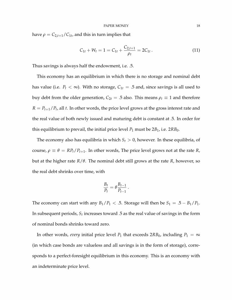
PAPER MONEY 18
have ρ = C2,t+1/C1t, and this in turn implies that
C1t + Wt = 1 = C1t +C2,t+1
ρt= 2C1t . (11)
Thus savings is always half the endowment, i.e. .5.
This economy has an equilibrium in which there is no storage and nominal debt
has value (i.e. Pt < ∞). With no storage, C1t = .5 and, since savings is all used to
buy debt from the older generation, C2t = .5 also. This means ρt ≡ 1 and therefore
R = Pt+1/Pt, all t. In other words, the price level grows at the gross interest rate and
the real value of both newly issued and maturing debt is constant at .5. In order for
this equilibrium to prevail, the initial price level P1 must be 2B1, i.e. 2RB0.
The economy also has equilibria in which St > 0, however. In these equilibria, of
course, ρ ≡ θ = RPt/Pt+1. In other words, The price level grows not at the rate R,
but at the higher rate R/θ. The nominal debt still grows at the rate R, however, so
the real debt shrinks over time, with
Bt
Pt= θ
Bt−1
Pt−1.
The economy can start with any B1/P1 < .5. Storage will then be S1 = .5 − B1/P1.
In subsequent periods, St increases toward .5 as the real value of savings in the form
of nominal bonds shrinks toward zero.
In other words, every initial price level P1 that exceeds 2RB0, including P1 = ∞
(in which case bonds are valueless and all savings is in the form of storage), corre-
sponds to a perfect-foresight equilibrium in this economy. This is an economy with
an indeterminate price level.
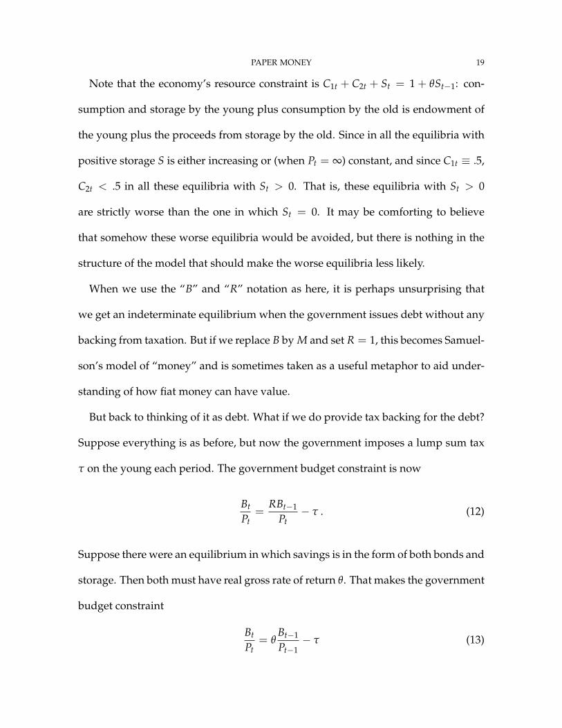
PAPER MONEY 19
Note that the economy’s resource constraint is C1t + C2t + St = 1 + θSt−1: con-
sumption and storage by the young plus consumption by the old is endowment of
the young plus the proceeds from storage by the old. Since in all the equilibria with
positive storage S is either increasing or (when Pt = ∞) constant, and since C1t ≡ .5,
C2t < .5 in all these equilibria with St > 0. That is, these equilibria with St > 0
are strictly worse than the one in which St = 0. It may be comforting to believe
that somehow these worse equilibria would be avoided, but there is nothing in the
structure of the model that should make the worse equilibria less likely.
When we use the “B” and “R” notation as here, it is perhaps unsurprising that
we get an indeterminate equilibrium when the government issues debt without any
backing from taxation. But if we replace B by M and set R = 1, this becomes Samuel-
son’s model of “money” and is sometimes taken as a useful metaphor to aid under-
standing of how fiat money can have value.
But back to thinking of it as debt. What if we do provide tax backing for the debt?
Suppose everything is as before, but now the government imposes a lump sum tax
τ on the young each period. The government budget constraint is now
Bt
Pt=
RBt−1
Pt− τ . (12)
Suppose there were an equilibrium in which savings is in the form of both bonds and
storage. Then both must have real gross rate of return θ. That makes the government
budget constraint
Bt
Pt= θ
Bt−1
Pt−1− τ (13)
PAPER MONEY 20
This is a stable difference equation in Bt/Pt. If it starts operation at t = 0, we will
have
Bt
Pt=
t−1
∑s=0
−τθs + θt B0
P0. (14)
But notice that, since θ < 1, the right-hand side of this expression eventually be-
comes negative, converging as t → ∞ to −τ/(1− θ). This means that from the point
of view of a representative individual in this economy, wealth in the form of govern-
ment debt holdings is insufficient to finance the individual’s future tax obligations.
This implies a desire for increased savings, putting downward pressure on prices,
and thus pushing the volume of real debt back up toward the zero-storage value.
If there is no storage, the rate of return on debt can be positive. The tax is recog-
nized by individual agents as reducing their wealth, so first-period consumption is
reduced. Formally, the private budget constraint in the first period is now
C1,t +Bt
Pt+ τ = 1 . (15)
We will still have, from the first-order conditions, RPt/Pt+1 = ρt = C2,t+1/Ct, where
ρt is just notation for the real rate of return. Using these last two expressions to
rewrite the first-period budget constraint, we have
C1t + τ +C2,t+1
ρt= 1 = C1t +
ρtC1t
ρt+ τ . (16)
Thus
C1t =1 − τ
2,
PAPER MONEY 21
with, as usual with log utility, first-period consumption being half of total wealth
1 − τ. With no storage, C1t + C2t = 1, which implies
C2t =1 + τ
2. (17)
Note that in this unique equilibrium, the utility of each generation is log(1 − τ) +
log(1 + τ) + 2 log(1/2), which is less than the upper bound of 2 log(1/2). Thus
with τ = 0, the utility-maximizing equilibrium exists, but is not unique, while small
positive values of τ make equilibrium unique, and can approach the utility of the
optimum for small τ.
The debt valuation equation holds in these equilibria. The gross real interest rate
is ρt = C2,t+1/C1t ≡ (1 + τ)/(1 − τ). From the government budget constraint, then,
we see that
Bt
Pt= ρt−1
Bt−1
Pt−1− τ ,
and since B/P = C2/ρ is constant in the equilibrium,
Bt
Pt=
τ
ρ − 1. (18)
Note that as τ approaches zero, B/P does not approach zero, as this formula might
suggest. ρ = C2/C1 = (1 + τ)/(1 − τ) in equilibrium and substituting this for ρ in
(18) gives us
Bt
Pt=
1 − τ
2. (19)
Because ρ → 1 as τ → 0, in other words, real debt converges to one half, its value
in the utility-maximizing equilibrium, as τ → 0, even though the debt valuation
equation (18) continues to hold.
PAPER MONEY 22
To see how the initial price level is determined, we look at the initial government
budget constraint. R−1 and B−1 are given by history, so
B0
P0=
1 − τ
2=
R−1Bt−1
Pt− τ . (20)
This equation can be solved for a unique, positive value of P0, so long as Rt−1Bt−1 >
0. The subsequent sequence of prices is determined by the sequence of policy choices
for Rt, with higher Rt values producing higher inflation.
What if initial Rt−1Bt−1 = 0? So long as we maintain the constraint that B0 >
0, fiscal policy cannot then at t = 0 be simply to set τ to its constant value. The
old at time 0 in this case have no way to finance consumption. It is plausible then
to suppose that the government imposes the tax τ on the young, issues new debt
bought by the young, and uses the proceeds to provide a subsidy to the time-0 old.
From that point on the equilibrium would be as we have calculated above.
III.2. Fiscal backup for a Taylor rule. Cochrane (2007) has argued against attempts
to claim a determinate price level in models with Taylor-rule monetary policy by
invoking “fiscal backing” that comes into play only off the equilibrium path. I don’t
understand his reasoning, but in any case the simple model of this section shows
that we can also justify uniqueness of the price level with a Taylor rule by invoking
fiscal backing that is always in play, even in equilibrium, but is negligibly small in
size. The equilibrium is then arbitrarily close to that of the model without fiscal
backing. In this and the preceding model, we conclude that the existence of fiscal
backing is important for stable prices, but that if market perception of the backing
PAPER MONEY 23
is there, the size of the backing can be quite small in equilibrium. Institutions like
those in the EMU that make it unclear where the fiscal backing would come from,
or even whether it exists, are destabilizing; yet in normal times, because large fiscal-
backing interventions do not occur in equilibrium, it is easy for the importance of
fiscal backing to be lost sight of.
The model is very simple, a continuous time extension of Leeper’s (1991) original
framework. The monetary policy rule is
r = γ(θ p − (r − ρ)
). (21)
This makes the nominal interest rate r respond with a delay (larger γ means less
delay) to inflation p. The “Taylor principle” that the interest rate should eventually
respond more than one for one to inflation changes corresponds here to θ > 1.
We assume a constant real rate ρ and a no-risk-aversion Fisher equation connecting
a constant real rate ρ and the nominal rate:
r = ρ + ˆp . (22)
The ˆp notation represents the right time derivative of the expected path of the log of
the price level. On a perfect foresight solution path, ˆp = p at all dates after the initial
date, but p can move discontinuously at the initial date. These two equations (21)
and (22) can be solved to yield a second order differential equation in p:
p = γ(θ − 1) p , (23)
PAPER MONEY 24
which holds after the initial date t = 0 on any perfect foresight equilibrium path.
With θ > 1, this is an unstable differential equation, with solutions of the form pt =
p0eγ(θ−1)t.
Leeper assumed that such explosive paths for the price level were not equilibrium
paths and focused on the one stable solution to the equation, p ≡ 0. On such a path
r = ρ from (22). From (21) this implies also that r = 0. The policy equation (21),
since it holds in actual (not expected-right) derivatives, implies that the time path of
r − γθp is differentiable, even at the initial date t = 0, but this leaves it possible that
both p and r jump discontinuously at t = 0, so long as the jumps satisfy ∆r = γθ∆p.
This makes the initial price level determinate. Using r−0 , p−0 to indicate the left limits
of these variables at time 0 (i.e. their pre-jump values), we have
∆r0 = ρ − r−0 = γθ(p0 − p−0 ) = γθ∆p0 . (24)
This equation can be solved for a unique value of p0 (right limit of the log of the price
level at time 0) as a function of ρ, r−0 , and p−0 .
If the initial price level should be below this level, r and thus ˆp would also be
lower, which implies inflation tends to −∞ at an exponential rate. The policy rule
(21) cannot possibly be maintained on such a path, as it would require pushing r
to negative values. It is natural to suppose that there would be a shift in the rule
at very low inflation rates, with fiscal policy ruling out such a path. If the initial
price level and inflation rate are above the steady state level, the inflation rate rises
at an exponential rate. The opportunity costs of holding non-interest-bearing money
balances become arbitrarily high. If real balances are essential (utility is driven to −∞
PAPER MONEY 25
as M/P → 0), these explosive paths may be viable equilibria. If not, there may be
an upper bound on the interest rate above which real balances become zero. Paths
on which real balances shrink to zero in finite time may also be viable equilibria.
Here again, though, we can postulate a shift in policy at very high inflation rates
that eliminates these unstable paths, while leaving the stationary p = 0 equilibrium
viable.
Cochrane finds these hypothetical policy shifts at high and low inflation rates,
which then never are observed in equilibrium, implausible. But suppose we add
a government budget constraint and fiscal policy, as did Leeper. The budget con-
straint, with real debt (not log of real debt) denoted as b and primary surplus de-
noted as τ, is
b = (r − p)b − τ . (25)
A version of what Leeper calls a passive fiscal policy is
τ = −ϕ0 + ϕ1b . (26)
Along a perfect foresight path, where r = ρ + p, this gives us
b = ρb + ϕ0 − ϕ1b . (27)
With ϕ1 > ρ, this is a stable equation in b. No matter what the equilibrium time path
of p, real debt converges to ϕ0/(ϕ1 − ρ). This equation can therefore play no role in
determining the price level, and thus cannot resolve the indeterminacy.
PAPER MONEY 26
But what if we add to the right hand side of (26) a positive response of the primary
surplus to inflation, i.e. replace (26) with
τ = −ϕ0 + ϕ1b + ϕ2π ? (28)
Then (27) becomes
b = (ρ − ϕ1)b + ϕ0 − ϕ2π . (29)
The three-equation differential equation system formed by (21), (22) and (29) is re-
cursive, since b appears only in the last equation. That means that the solution paths
that make π explode up or down that we observed when considering the first two
equations alone are still mathematical solution paths for the three-equation system.
But now notice what happens to b along a path on which p → ∞. From the debt
equation (29) we see that on such a path b eventually becomes negative and more
negative over time. This implies that b goes to zero in finite time. From the point of
view of private agents in the economy, since we assume they can’t borrow from the
government, this means that their future tax obligations exceed their wealth in the
form of government debt, and thus that they cannot finance their planned consump-
tion with the income and wealth they have. They will therefore reduce consumption
and try to save. If they truly have perfect foresight, this would instantly, at the initial
date t = 0, bring p0 back to the level consistent with stability. If it takes agents some
time to realize what kind of a path they are on, the adjustment might come with
a delay, still producing the same reversion to the stable solution. Unstable paths
with accelerating deflation can also be ruled out. On such paths, real debt would
PAPER MONEY 27
rise without bound, while primary surpluses shrank and eventually became nega-
tive. Now people would see their wealth in the form of government debt growing
without bound, with no offsetting increase in future tax obligations. They would
therefore spend, raising prices, bringing the economy back to its stable path.
These arguments do not depend on the size of ϕ2, so long as it is positive. In equi-
librium, π will be zero or (if people are imperfectly foresighted, or if we add random
disturbances to the system) fluctuate in a narrow range. If ϕ2 is small enough, its
presence might be difficult to detect from data. In any case its presence would have
no effect on the first two equations of the system or on the equilibrium time path
of prices and interest rates, except for its elimination of the unstable solutions as
equilibria of the economy.
III.3. Debt as a fiscal cushion. Barro (1979) showed in a simple, stylized model that
in the presence of distorting taxation it is not optimal to rapidly pay off public debt,
because the dead-weight losses from heavy initial taxation to reduce the debt are
not offset by the present value of lower future dead-weight losses after the debt is
reduced. Instead, in his model, debt and tax revenue optimally follow a martin-
gale processes, with Etbt+1 = bt, Etτt+1 = τt. (Here τ is total tax revenue.) In his
framework, τ increases with increases in b. Lucas and Stokey (1983) showed that
when the government can issue contingent liabilities, it is actually optimal for taxes
to be set without reference to the current level of debt. Chari, Christiano, and Kehoe
(1994) showed that monetary policy, by determining inflation, can create appropriate
contingencies in the return to debt. I showed (2001) that if these insights are brought
PAPER MONEY 28
back to Barro’s stylized framework, we get a simple and stark conclusion — τ should
be constant, with b brought in line with stochastically fluctuating future government
spending by surprise inflation and deflation.
However, these results all depend on surprise inflation and deflation being cost-
less. In a Keynesian model with sticky prices or wages, or in a model with incom-
plete markets and borrowing and lending via standard debt contracts in nominal
terms, surprise inflation has a substantial cost. Schmitt-Grohé and Uribe (2001)
showed that in a New Keynesian model with one-period government debt, opti-
mal policy is much closer to Barro’s initial prescription than to a constant-τ policy. It
makes a great deal of difference, though, whether government debt is long or short
term. When debt is short, as in Schmitt-Grohé and Uribe’s setup, inflation or defla-
tion is the only way to change its market value in response to government spending
surprises. But if the debt is long term, large changes in the value of the debt can
be produced by changes in the nominal interest rate, with much smaller changes
in inflation. Interest rates fluctuate widely and their fluctuations are not thought
of as very costly, while price fluctuations may generate inefficient output and em-
ployment fluctuations. The model of this section revisits Barro’s framework, adding
endogenous price determination and allowing for short or long debt. It concludes
that substantial use of the nominal debt fiscal cushion to limit tax fluctuations may
be optimal if debt maturity is long.
Following Barro, we model the government as wanting to minimize the dead-
weight loss from taxation, modeled as proportional to τ2, the square of total revenue.
PAPER MONEY 29
But we add to his specification a concern with wide swings in inflation, leading to
the objective function
−12
E
[∞
∑t=0
βt
(τ2 + θ
(Pt
Pt−1− 1)2)]
. (30)
It simplifies notation for us to use the single symbol νt = Pt−1/Pt to denote the
inverse of the gross inflation rate from this point on. There is a constant real interest
rate, and private sector behavior requires the real rate to match the expected nominal
return on a bond:
RtEtνt+1 = ρ . (31)
The government budget constraint is
bt = Rt−1νtbt−1 − τt + gt , (32)
where b is real debt and gt is government spending, which we treat as an exogenous
stochastic process. The government then maximizes (30) by choosing R, P, b, and τ
subject to the two constraints (31) and (32). The first order conditions for an optimum
are
∂τ : τt = λt (33)
∂b : λt = βRtEt[νt+1λt+1] (34)
∂R : µtEtνt+1 = βEt[νt+1λt+1]bt (35)
∂ν : θ · (νt − 1) = −λtRt−1bt−1 + µt−1Rt−1ρ . (36)
PAPER MONEY 30
These first order conditions look complicated, but when θ = 0, so that there is no
cost to inflation, they collapse to a surprisingly simple solution. To keep things neat,
we assume βρ = 1. From the b and R FOC’s and the Fisher equation (31) we can
derive
btλt = µtρ . (37)
Substituting into the ν first order condition, we arrive at
θ · (νt − 1) = (−λt + λt−1)Rt−1bt−1 = (τt − τt−1)Rt−1bt−1 . (38)
If θ = 0, this lets us conclude that τt = τt−1, so long as Rt−1 and bt−1 are both posi-
tive. With τt constant and gt exogenous and stochastic, (31) is an unstable equation.
Feasibility (b > 0) and transversality (bt → 0 while future τ’s are constant cannot be
optimal) imply that b must not explode. This implies that we can solve the budget
constraint (32) forward to produce
bt =τ
ρ − 1− Et
[∞
∑s=1
ρ−sgt+s
]. (39)
In the special case where g is i.i.d., b is constant. b is maintained at these stability-
consistent values by fluctuations in νt, the inverse inflation rate, that offset the effects
of g on the real value of the debt.
So far, we have derived an analogue in this simple model of the Lucas-Stokey
result, by setting θ = 0. We can also consider θ = ∞, i.e. a case where the price level
is kept constant and only real government debt exists. Then we drop the ν first order
condition, because ν is no longer freely chosen, and use the fact that νt ≡ 1. Then the
PAPER MONEY 31
b first order condition lets us conclude that Etτt+1 = τt, and we are back to Barro’s
conclusion (since we are now back to Barro’s model, which had only real debt).
The cases of most interest, though, are those with 0 < θ < ∞. For these cases,
we want to contrast this version of the model with one in which government debt is
not only nominal, but long term. We will consider the extreme case of consol debt,
which pays a stream of one “dollar” per period forever, never returning principal.
The number of consols held by the public is At and the price, in dollars, of a consol
is Qt. (So 1/Qt is the long term interest rate). Then the Fisher equation requires that
the expected one-period yield on a consol be equal to ρ, i.e.
Et
[Qt+1νt+1 + 1
Qt
]= ρ , (40)
and the budget constraint becomes
bt =AtQt
Pt= bt−1
(Qtνt + 1
Qt−1
)− τt + gt . (41)
Because these systems with non-trivial θ become difficult to handle analytically, we
omit laying out the first order conditions for the consol-debt case, and we solve,
numerically, locally linearized versions of both the short debt and long debt models.
We assume gt is independent across time, with constant mean Egt = g = 1. We set
ρ = β−1 = 1.1, and τ = 2 in the initial steady state. Because this makes τ − g = 1,
and the net real rate ρ − 1 = .1, initial steady state real debt b = 10.
With real debt, as in Barro’s original framework (i.e. θ = ∞), a unit increase in
gt above its mean g requires τ and b to move to new levels that could be sustained
forever if future g values reverted to g. So with our parameter settings, 10/11 of
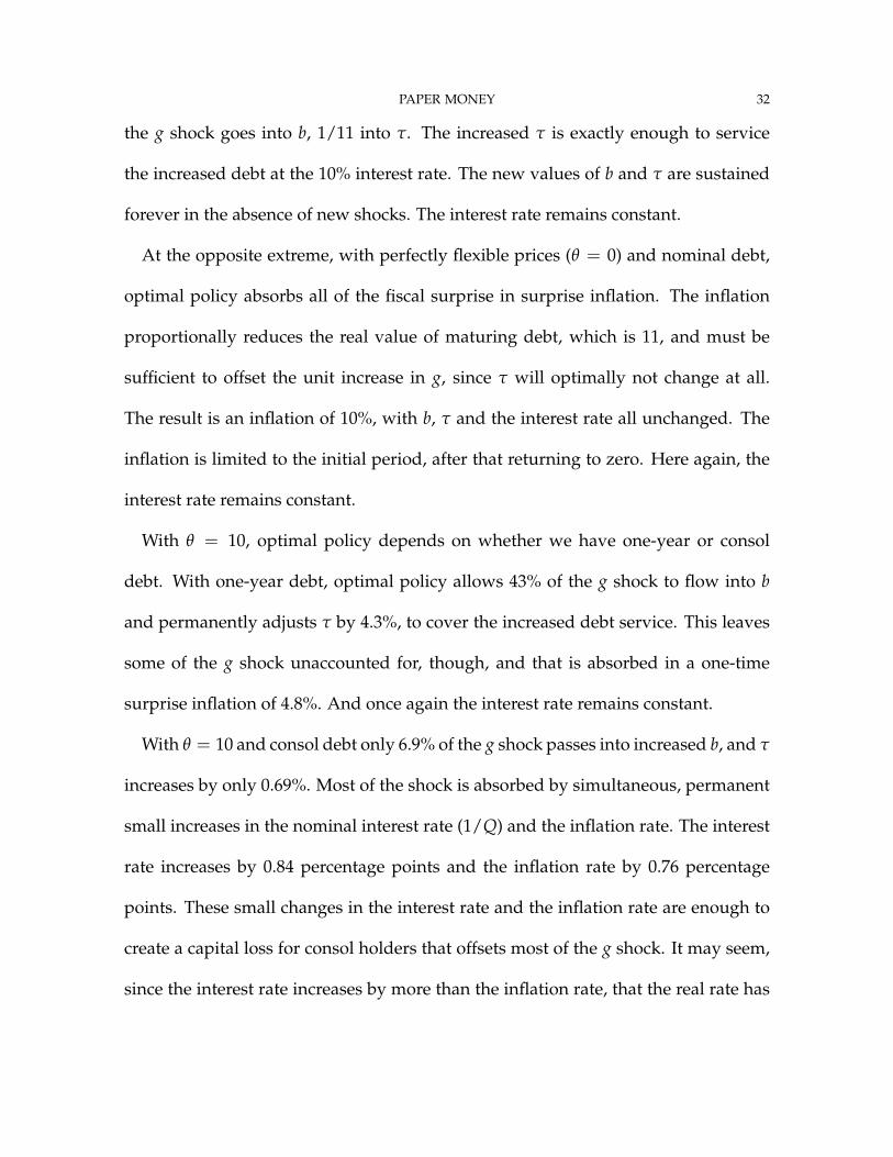
PAPER MONEY 32
the g shock goes into b, 1/11 into τ. The increased τ is exactly enough to service
the increased debt at the 10% interest rate. The new values of b and τ are sustained
forever in the absence of new shocks. The interest rate remains constant.
At the opposite extreme, with perfectly flexible prices (θ = 0) and nominal debt,
optimal policy absorbs all of the fiscal surprise in surprise inflation. The inflation
proportionally reduces the real value of maturing debt, which is 11, and must be
sufficient to offset the unit increase in g, since τ will optimally not change at all.
The result is an inflation of 10%, with b, τ and the interest rate all unchanged. The
inflation is limited to the initial period, after that returning to zero. Here again, the
interest rate remains constant.
With θ = 10, optimal policy depends on whether we have one-year or consol
debt. With one-year debt, optimal policy allows 43% of the g shock to flow into b
and permanently adjusts τ by 4.3%, to cover the increased debt service. This leaves
some of the g shock unaccounted for, though, and that is absorbed in a one-time
surprise inflation of 4.8%. And once again the interest rate remains constant.
With θ = 10 and consol debt only 6.9% of the g shock passes into increased b, and τ
increases by only 0.69%. Most of the shock is absorbed by simultaneous, permanent
small increases in the nominal interest rate (1/Q) and the inflation rate. The interest
rate increases by 0.84 percentage points and the inflation rate by 0.76 percentage
points. These small changes in the interest rate and the inflation rate are enough to
create a capital loss for consol holders that offsets most of the g shock. It may seem,
since the interest rate increases by more than the inflation rate, that the real rate has
PAPER MONEY 33
increased, even though we have assumed constant ρ. However, this happens only
because of the definition of the “nominal rate” as 1/Q. This is a good approximation
when there is no inflation, but when there is steady inflation, as in the wake of this
shock, a consol’s constant stream of nominal payments is front-loaded in real terms,
so that in fact the constant real rate is preserved by this combination of permanent
changes in inflation and 1/Q.
The response to the g shock in the four cases we have discussed in the preceding
paragraphs is displayed in Figure 2. Each column of plots shows the time path of
changes in the four variables listed on the left side of the chart, in the case labeled at
the top of the column. Note that the 1-year debt case with θ = 10 is about halfway
between the pure real debt case of Barro and the flex-price case. The consol case
is very close to the flex-price case for the time paths of the real variables b and τ,
though its time path for inflation and interest rates is quite different.
The point of this comparison is not to claim that a combination of long debt and
low response of taxes to fiscal shocks is optimal. The model is extremely stylized,
and the costs of inflation have been calibrated only to a value that makes contrasts
between cases easy to see. As is by now well understood, the first-order accurate so-
lution obtained as here by local linearization does not allow us directly to compute
expected welfare, even for the stylized objective function. Since both taxes and infla-
tion vary much less in the consol solution, it seems likely that it delivers higher wel-
fare, but because the budget constraint is nonlinear, we can’t be certain of this. The
amount of shock absorption available from surprise changes in prices and interest
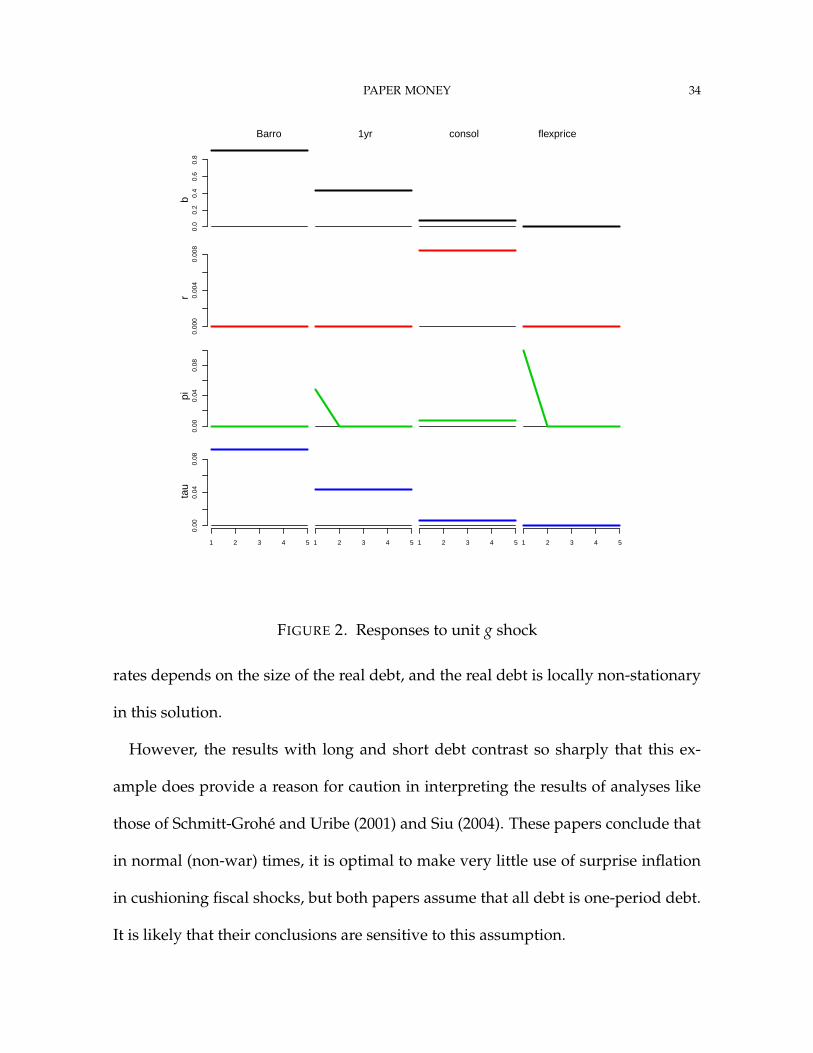
PAPER MONEY 34
0.0
0.2
0.4
0.6
0.8
0.00
00.
004
0.00
80.
000.
040.
080.
000.
040.
08
1 2 3 4 5 1 2 3 4 5 1 2 3 4 5 1 2 3 4 5
Barro 1yr consol flexprice
br
pita
u
FIGURE 2. Responses to unit g shock
rates depends on the size of the real debt, and the real debt is locally non-stationary
in this solution.
However, the results with long and short debt contrast so sharply that this ex-
ample does provide a reason for caution in interpreting the results of analyses like
those of Schmitt-Grohé and Uribe (2001) and Siu (2004). These papers conclude that
in normal (non-war) times, it is optimal to make very little use of surprise inflation
in cushioning fiscal shocks, but both papers assume that all debt is one-period debt.
It is likely that their conclusions are sensitive to this assumption.
PAPER MONEY 35
IV. CONCLUSION
The kinds of models that have been the staple of undergraduate macroeconomics
teaching, with price level determined by balance between “money supply” and “money
demand”, and money supply described using the “money multiplier”, are obsolete
and provide little insight into the policy issues facing fiscal and monetary authorities
in the last few years. There are relatively simple models available, though, that could
be taught in undergraduate and graduate courses and that would allow discussion
of current policy issues using clearer analytic foundations.
DATA APPENDIX
Surprise gains and losses on the debt. The calculations for Figure 1 were done as
follows. The unanticipated gains or losses were formed as
Bt(1 − πt) + St − (1 + rt−1)Bt−1 .
Bt is the market value of the marketable US debt, as calculated by the Federal Re-
serve Bank of Dallas. This series has recently been updated by them, and they sent
me the updated version. The time unit for this equation is one year. St is the pri-
mary surplus, calculated from the US national income and product accounts, Table
3.2, as net lending or borrowing, line 39, plus interest payments, line 22. rt is the
one-year interest rate on treasury securities at the beginning of the year. πt is the
error in a forecast of inflation for year t made at the beginning of year t. The logic
is that holders of debt at the beginning of the year expected their holdings to grow
to (1 + rt−1)Bt−1 at the end of the year. Some of the debt is retired, though, and that
PAPER MONEY 36
is accounted for by the St term. And the real value of the debt undergoes surprising
change because of errors in predicting inflation. This formula is at best approximate
for several reasons. One-year government debt carries some liquidity premium, and
indeed Figure 1 shows that “surprises” in yield are on average positive, probably
because of the liquidity premium. Some debt is of maturity less than one year, so as
information about inflation accumulates during the year, interest rates on these com-
ponents of the debt can compensate. Thus some gains and losses that were actually
anticipated within the year are treated as unanticipated in this formula. The calcula-
tion of the market value of the debt involves some interpolation and approximation,
though the quantity used here, total marketable debt, is the least affected by these
considerations of the three concepts reported by the Dallas Fed.
Total marketable debt excludes “debt” of the government to itself in Treasury ac-
counts, but it does include treasury securities held by the Federal Reserve system.
Since the Fed is not a profit or utility maximizing agent, it would be better to include
it as part of the government, and the Dallas Fed does report a concept that excludes
Fed holdings. But if the Fed is part of the government, then its interest-bearing li-
abilities are part of the public debt and changes in its holdings of debt that do not
correspond to changes in non-interest-bearing liabilities are part of the primary sur-
plus. These considerations are quantitatively important in recent years, with the
expansion of the Fed’s balance sheet and its beginning to pay interest on reserves.
Surprise inflation is not easy to quantify. During the late 1970’s and early 80’s
inflation underwent wide swings that were not well tracked by statistical models fit
PAPER MONEY 37
to historical data. Probably expectations about future inflation were diverse during
1973-83, not well summarized by any single number. A Bayesian VAR model using
the log of the chained PCE deflator and the one-year interest rate gives reasonable-
looking results, but its time series of forecast errors is quite different from what is
obtained by predicting inflation over year t as simply equal to inflation over year t −
1, and the sum of squared forecast errors is nearly the same for the two forecasting
methods. The simple πt = πt−1 forecasts were used to produce the figure, but the
figure would have looked noticeably different if the VAR forecasts had been used.
Hall and Sargent (2011) calculate ex post real and nominal returns on US govern-
ment debt by a method that does not rely on the NIPA data to compute a primary
surplus. It is possible to use their ex post real returns, together with the one-year
interest rate series and the inflation forecast error series and a series for the level of
the debt, to compute the same concept shown in Figure 1. I made those calculations,
and they produce fluctuations of the same order of magnitude as in the figure, but
again with a different time profile.
Sources for Table 1. These data were drawn from the international component of
the FRED database provided by the Federal Reserve Bank of St. Louis. The interest
rates are those labeled “government bond” interest rates. The debt to GDP ratios are
provided in that form by FRED.
REFERENCES
BARRO, R. J. (1979): “On the Determination of the Public Debt,” Journal of Political
Economy, 87(5:part 1), 940–971.
PAPER MONEY 38
CHARI, V., L. J. CHRISTIANO, AND P. J. KEHOE (1994): “Optimal Fiscal Policy in a
Business Cycle Model,” Journal of Political Economy, 102(4), 617–652.
COCHRANE, J. H. (1998): “A Frictionless View of US Inflation,” NBER Macroeco-
nomics Annual, 13, 323–384.
(2007): “Inflation Determination with Taylor Rules: A Critical Re-
view,” Discussion paper, Graduate School of Business, University of Chicago,
http://faculty.chicagogsb.edu/john.cochrane/research/Papers/.
DAVIG, T., AND E. M. LEEPER (2006): “Fluctuating Macro Policies and the Fiscal
Theory,” NBER Macroeconomics Annual, pp. 247–298.
HALL, G. J., AND T. J. SARGENT (2011): “Interest Rate Risk and Other Determinants
of Post-WWII US Government Debt/GDP Dynamics,” American Economic Journal:
Macroeconomics 3, 3, 192–214.
LEEPER, E. M. (1991): “Equilibria Under ‘Active’ and ‘Passive’ Monetary And Fiscal
Policies,” Journal of Monetary Economics, 27, 129–47.
LOYO, E. (2000): “Tight Money Paradox on the Loose: A Fiscalist Hy-
perinflation,” Discussion paper, John F. Kennedy School of Government,
http://sims.princeton.edu/yftp/Loyo/LoyoTightLoose.pdf.
LUCAS, R. E. J., AND N. STOKEY (1983): “Optimal Fiscal and Monetary Policy in an
Economy without Capital,” Journal of Monetary Economics, 12(1), 55–93.
SCHMITT-GROHÉ, S., AND M. URIBE (2001): “Optimal Fiscal and Monetary Pol-
icy Under Sticky Prices,” Discussion paper, Rutgers University and University of
Pennsylvania.
PAPER MONEY 39
SIMS, C. A. (1999): “The Precarious Fiscal Foundations of EMU,” De Economist,
147(4), 415–436, http://www.princeton.edu/~sims/.
(2001): “Fiscal Consequences for Mexico of Adopting the Dollar,” Journal of
Money, Credit, and Banking, 33(2,part2), 597–616.
(2004): “Fiscal Aspects of Central Bank Independence,” in European Monetary
Integration, ed. by H.-W. Sinn, M. Widgrén, and M. Köthenbürger, CESifo seminar
series, chap. 4, pp. 103–116. MIT Press, Cambridge, Massachusetts.
(2005): “Limits to Inflation Targeting,” in The Inflation-Targeting Debate, ed.
by B. S. Bernanke, and M. Woodford, vol. 32 of National Bureau of Economic Re-
search Studies in Business Cycles, chap. 7, pp. 283–310. University of Chicago Press,
Chicago and London, presented at an NBER conference in Miami, January 2003.
(2012): “Gaps in the Institutional Structure of the Euro
Area,” in Public Debt, Monetary Policy and Financial Stability, no. 16
in Financial Stability Review, pp. 217–223. Banque de France,
http://sims.princeton.edu/yftp/EuroGaps/EuroGaps.pdf.
SIU, H. E. (2004): “Optimal fiscal and monetary policy with sticky prices,” Journal of
Monetary Economics, 51, 575–607.
WALLACE, N. (1981): “A Modigliani-Miller Theorem for Open-Market Operations,”
The American Economic Review, 71(3), 267–274.
WOODFORD, M. (1995): “Price Level Determinacy Without Control of a Monetary
Aggregate,” Carnegie-Rochester Conference Series on Public Policy, 43, 1–46.