Paper folding myth Repeated Minimum: Code

Paper folding myth

• no paper can be foldedmore than 7 times

•WHY?

Sorting

Practice with Analysis

Repeated Minimum

• Search the list for the minimum element.

• Place the minimum element in the first position.

• Repeat for other n-1 keys.

• Use current position to hold current minimum to avoid large-scale movement of keys.

Repeated Minimum: Code

for i := 1 to n-1 dofor j := i+1 to n doif L[i] > L[j] thenTemp = L[i];L[i] := L[j];L[j] := Temp;

endifendfor

endfor

Fixed n-1 iterations

Fixed n-i iterations

Repeated Minimum: Analysis

Doing it the dumb way:

∑−

=

−1

1

)(n

i

in

The smart way: I do one comparison when i=n-1, two when i=n-2, … , n-1 when i=1.

)(2

)1( 21

1

nnn

kn

k

Θ∈−

=∑−

=

Bubble Sort

• Search for adjacent pairs that are out of order.

• Switch the out-of-order keys.

• Repeat this n-1 times.

• After the first iteration, the last key is guaranteed to be the largest.

• If no switches are done in an iteration, we can stop.

Bubble Sort: Code

for i := 1 to n-1 doSwitch := False;for j := 1 to n-i doif L[j] > L[j+1] thenTemp = L[j];L[j] := L[j+1];L[j+1] := Temp;Switch := True;

endifendforif Not Switch then break;

endfor

Worst case n-1 iterations

Fixed n-i iterations

Bubble Sort Analysis

Being smart right from the beginning:

)(2

)1( 21

1

nnn

in

i

Θ∈−

=∑−

=

Insertion Sort I

• The list is assumed to be broken into a sorted portion and an unsorted portion

• Keys will be inserted from the unsorted portion into the sorted portion.

Sorted Unsorted

Insertion Sort II

• For each new key, search backward through sorted keys

• Move keys until proper position is found

• Place key in proper position

Moved

Insertion Sort: Code

for i:= 2 to n dox := L[i];j := i-1;while j<0 and x < L[j] doL[j-1] := L[j];j := j-1;

endwhileL[j+1] := x;

endfor


Worst case i-1 comparisons

Insertion Sort: Analysis

•Worst Case: Keys are in reverse order

• Do i-1 comparisons for each new key, where i runs from 2 to n.

• Total Comparisons: 1+2+3+ … + n-1

( )in n

ni

n

=

−

∑ =−

∈1

121

2

( )Θ

Insertion Sort: Average I

• Assume: When a key is moved by the While loop, all positions are equally likely.

• There are i positions (i is loop variable of for loop) (Probability of each: 1/i.)

• One comparison is needed to leave the key in its present position.

• Two comparisons are needed to move key over one position.

Insertion Sort Average II

• In general: k comparisons are required to move the key over k-1 positions.

• Exception: Both first and second positions require i-1 comparisons.

1 2 3 ... ii-1i-2

i-1 i-1 i-2 3 2 1

Position

...

...

Comparisons necessary to place key in this position.

Insertion Sort Average III

( )∑−

=

−+1

1

111i

j

ii

ji

Average Comparisons to place one key

i

i

i

ii

iij

i

i

i

1

2

11

2

2

2

)1(111

1 1

1

−+

=−+−

=

−+= ∑

−

=

Solving

Insertion Sort Average IV

For All Keys:

∑∑∑∑====

−+=

−

+=

n

i

n

i

n

i

n

i ii

i

in

2222

11

2

1

2

11

2

1)A(

∑=

−−+−+

=n

i i

nnn

2

1

2

1

4

2

2

1

4

)1(

( )2

2

2 11

4

3

4n

i

nn n

i

Θ∈−−+= ∑=

Optimality Analysis I

• To discover an optimal algorithm we need to find an upper and lower asymptotic bound for a problem.

• An algorithm gives us an upper bound. The worst case for sorting cannot exceed Θ(n2) because we have Insertion Sort that runs that fast.

• Lower bounds require mathematical arguments.

Optimality Analysis II

• Making mathematical arguments usually involves assumptions about how the problem will be solved.

• Invalidating the assumptions invalidates the lower bound.

• Sorting an array of numbers requires at least Θ(n) time, because it would take that much time to rearrange a list that was rotated one element out of position.

Rotating One Element

2nd3rd4th

nth1st

2nd3rd

n-1stnth

1stn keys mustbe moved

Θ(n) time

Assumptions:

Keys must be movedone at a time

All key movements takethe same amount of time

The amount of timeneeded to move one keyis not dependent on n.

Other Assumptions

• The only operation used for sorting the list is swapping two keys.

• Only adjacent keys can be swapped.

• This is true for Insertion Sort and Bubble Sort.

• Is it true for Repeated Minimum? What about if we search the remainder of the list in reverse order?

Inversions

• Suppose we are given a list of elements L, of size n.

• Let i, and j be chosen so 1≤i<j≤n.

• If L[i]>L[j] then the pair (i,j) is an inversion.

1 2 3 45 6 7 8 910

Inversion Inversion Inversion

Not an Inversion

Maximum Inversions

• The total number of pairs is:

• This is the maximum number of inversions in any list.

• Exchanging adjacent pairs of keys removes at most one inversion.

2

)1(

2

−=

nnn

Swapping Adjacent Pairs

Swap Red and Green

The relative position of the Redand blue areas has not changed.No inversions between the red keyand the blue area have been removed.The same is true for the red key andthe orange area. The same analysis canbe done for the green key.

The only inversionthat could be removedis the (possible) onebetween the red andgreen keys.

Lower Bound Argument

• A sorted list has no inversions.

• A reverse-order list has the maximum number of inversions, Θ(n2) inversions.

• A sorting algorithm must exchange Θ(n2) adjacent pairs to sort a list.

• A sort algorithm that operates by exchanging adjacent pairs of keys must have a time bound of at least Θ(n2).

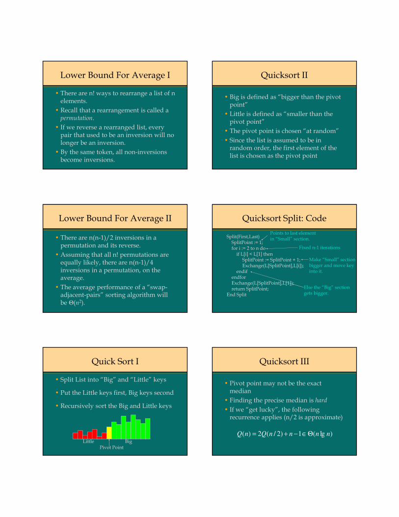
Lower Bound For Average I

• There are n! ways to rearrange a list of n elements.

• Recall that a rearrangement is called a permutation.

• If we reverse a rearranged list, every pair that used to be an inversion will no longer be an inversion.

• By the same token, all non-inversions become inversions.

Lower Bound For Average II

• There are n(n-1)/2 inversions in a permutation and its reverse.

• Assuming that all n! permutations are equally likely, there are n(n-1)/4 inversions in a permutation, on the average.

• The average performance of a “swap-adjacent-pairs” sorting algorithm will be Θ(n2).

Quick Sort I

• Split List into “Big” and “Little” keys

• Put the Little keys first, Big keys second

• Recursively sort the Big and Little keys

Little BigPivot Point

Quicksort II

• Big is defined as “bigger than the pivot point”

• Little is defined as “smaller than the pivot point”

• The pivot point is chosen “at random”

• Since the list is assumed to be in random order, the first element of the list is chosen as the pivot point

Quicksort Split: Code

Split(First,Last)SplitPoint := 1;for i := 2 to n doif L[i] < L[1] thenSplitPoint := SplitPoint + 1;Exchange(L[SplitPoint],L[i]);

endifendforExchange(L[SplitPoint],L[1]);return SplitPoint;

End Split


Points to last elementin “Small” section.

Else the “Big” sectiongets bigger.

Make “Small” sectionbigger and move keyinto it.

Quicksort III

• Pivot point may not be the exact median

• Finding the precise median is hard

• If we “get lucky”, the following recurrence applies (n/2 is approximate)

)lg(1)2/(2)( nnnnQnQ Θ∈−+=

Quicksort IV

• If the keys are in order, “Big” portion will have n-1 keys, “Small” portion will be empty.

• N-1 comparisons are done for first key

• N-2 comparisons for second key, etc.

• Result:

( )in n

ni

n

=

−

∑ =−

∈1

121

2

( )Θ

QS Avg. Case: Assumptions

•Average will be taken over Location of Pivot

•All Pivot Positions are equally likely

•Pivot positions in each call are independent of one another

QS Avg: Formulation

•A(0) = 0

• If the pivot appears at position i, 1≤≤≤≤i≤≤≤≤n then A(i-1) comparisons are done on the left hand list and A(n-i) are done on the right hand list.

•n-1 comparisons are needed to split the list

QS Avg: Recurrence

( )A i A n ii

n

( ) ( )− + −=

∑ 11

( ) ( )= + − + + − +A A n A A n( ) ( ) ( ) ( )0 1 1 2

( )A n A n n( ) ( )− + −1

+−−+−−+ ))1(()1)1(((... nnAnA

( )A n nn

A i A n ii

n

( ) ( ) ( )= − + − + −=

∑11

11

QS Avg: Recurrence II

( )A i A n ii

n

( ) ( )− + − ==

∑ 11

2 0 21

1

A A ii

n

( ) ( )+=

−

∑

A n nn

A ii

n

( ) ( ) ( )= +=

−

∑Θ2

1

1

QS Avg: Solving Recurr.

Guess: A n an n b( ) lg≤ + a>0, b>0

A n nn

A ii

n

( ) ( ) ( )= +=

−

∑Θ2

1

1

( )≤ + +=

−

∑Θ( ) lgnn

ai i bi

n2

1

1

( )= + + −=

−

∑Θ( ) lgna

ni i

b

nn

i

n2 21

1

1

QS Avg: Continuing

By Integration:

i i n n ni

n

lg lg=

−

∑ ≤ −1

12 21

2

1

8

QS Avg: Finally

( )A na

nn n n

b

nn n( ) lg ( )≤ −

+ − +

2 1

2

1

8

21

2 2Θ

≤ − + +an na

n b nlg ( )4

2 Θ

= − + +an na

n b nlg ( )4

2 Θ

≤ +an n blg

Merge Sort

• If List has only one Element, do nothing

• Otherwise, Split List in Half

• Recursively Sort Both Lists

• Merge Sorted Lists

The Merge Algorithm

Assume we are merging lists A and B into list C.

Ax := 1; Bx := 1; Cx := 1;while Ax ≤ n and Bx ≤ n doif A[Ax] < B[Bx] thenC[Cx] := A[Ax];Ax := Ax + 1;elseC[Cx] := B[Bx];Bx := Bx + 1;endifCx := Cx + 1;

endwhile

while Ax ≤ n doC[Cx] := A[Ax];Ax := Ax + 1;Cx := Cx + 1;

endwhilewhile Bx ≤ n doC[Cx] := B[Bx];Bx := Bx + 1;Cx := Cx + 1;

endwhile

Merge Sort: Analysis

• Sorting requires no comparisons

• Merging requires n-1 comparisons in the worst case, where n is the total size of both lists (n key movements are required in all cases)

• Recurrence relation:

( )W( ) W( / ) lgn n n n n= + − ∈2 2 1 Θ

Merge Sort: Space

• Merging cannot be done in place

• In the simplest case, a separate list of size n is required for merging

• It is possible to reduce the size of the extra space, but it will still be Θ(n)

Heapsort: Heaps

• Geometrically, a heap is an “almost complete” binary tree.

• Vertices must be added one level at a time from right to left.

• Leaves must be on the lowest or second lowest level.

• All vertices, except one must have either zero or two children.

Heapsort: Heaps II

• If there is a vertex with only one child, it must be a left child, and the child must be the rightmost vertex on the lowest level.

• For a given number of vertices, there is only one legal structure

Heapsort: Heap examples

Heapsort: Heap Values

• Each vertex in a heap contains a value

• If a vertex has children, the value in the vertex must be larger than the value in either child.

• Example:20

19 7

12 2 5 6

310

Heapsort: Heap Properties

• The largest value is in the root

• Any subtree of a heap is itself a heap

• A heap can be stored in an array by indexing the vertices thus:

• The left child of vertexv has index 2v andthe right child hasindex 2v+1

1

2 3

4 5 6 7

98

Heapsort: FixHeap

• The FixHeap routine is applied to a heap that is geometrically correct, and has the correct key relationship everywhere except the root.

• FixHeap is applied first at the root and then iteratively to one child.

Heapsort FixHeap Code

FixHeap(StartVertex)v := StartVertex;while 2*v ≤ n doLargestChild := 2*v;if 2*v < n thenif L[2*v] < L[2*v+1] thenLargestChild := 2*v+1;

endifendifif L[v] < L[LargestChild] ThenExchange(L[v],L[LargestChild]);v := LargestChild

elsev := n;

endifendwhile

end FixHeap

n is the size of the heap

Worst case run time isΘ(lg n)

Heapsort: Creating a Heap

• An arbitrary list can be turned into a heap by calling FixHeap on each non-leaf in reverse order.

• If n is the size of the heap, the non-leaf with the highest index has index n/2.

• Creating a heap is obviously O(n lg n).

• A more careful analysis would show a true time bound of Θ(n)

Heap Sort: Sorting

• Turn List into a Heap

• Swap head of list with last key in heap

• Reduce heap size by one

• Call FixHeap on the root

• Repeat for all keys until list is sorted

Sorting Example I

20

19 7

12 2 5 6

310

20 19 7 12 2 5 6 10 3

19 7

12 2 5 6

3

10

2019 7 12 2 5 6 103

Sorting Example II

19

7

12 2 5 6

3

10

2019 7 12 2 5 6 103

19

712

2 5 63

10

2019 712 2 5 6 103

Sorting Example III

19

712

2 5 6

3

10

2019 712 2 5 610 3

Ready to swap 3 and 19.

Heap Sort: Analysis

• Creating the heap takes Θ(n) time.

• The sort portion is Obviously Ο(nlgn)

• A more careful analysis would show an exact time bound of Θ(nlgn)

• Average and worst case are the same

• The algorithm runs in place

A Better Lower Bound

• The Θ(n2) time bound does not apply to Quicksort, Mergesort, and Heapsort.

• A better assumption is that keys can be moved an arbitrary distance.

• However, we can still assume that the number of key-to-key comparisons is proportional to the run time of the algorithm.

Lower Bound Assumptions

• Algorithms sort by performing key comparisons.

• The contents of the list is arbitrary, so tricks based on the value of a key won’t work.

• The only basis for making a decision in the algorithm is by analyzing the result of a comparison.

Lower Bound Assumptions II

• Assume that all keys are distinct, since all sort algorithms must handle this case.

• Because there are no “tricks” that work, the only information we can get from a key comparison is:

• Which key is larger

Lower Bound Assumptions III

• The choice of which key is larger is the only point at which two “runs” of an algorithm can exhibit divergent behavior.

• Divergent behavior includes, rearranging the keys in two different ways.

Lower Bound Analysis

•We can analyze the behavior of a particular algorithm on an arbitrary list by using a tree.

i,j

k,l m,n

q,p t,s r,w x,y

L[i]<L[j] L[i]>L[j]

L[k]<L[l] L[k]>L[l] L[m]<L[n] L[m]>L[n]

Lower Bound Analysis

• In the tree we put the indices of the elements being compared.

• Key rearrangements are assumed, but not explicitly shown.

• Although a comparison is an opportunity for divergent behavior, the algorithm does not need to take advantage of this opportunity.

The leaf nodes

• In the leaf nodes, we put a summary of all the key rearrangements that have been done along the path from root to leaf.

1->22->33->1

2->33->2

1->22->1

The Leaf Nodes II

• Each Leaf node represents a permutation of the list.

• Since there are n! initial configurations, and one final configuration, there must be n! ways to reconfigure the input.

• There must be at least n! leaf nodes.

Lower Bound: More Analysis

• Since we are working on a lower bound, in any tree, we must find the longest path from root to leaf. This is the worst case.

• The most efficient algorithm would minimize the length of the longest path.

• This happens when the tree is as close as possible to a complete binary tree

Lower Bound: Final

• A Binary Tree with k leaves must have height at least lg k.

• The height of the tree is the length of the longest path from root to leaf.

• A binary tree with n! leaves must have height at least lg n!

Lower Bound: Algebra

∑ ∑= =

==n

i

n

i

iin2 2

ln2ln

1lg!lg

∫ ∑ ∫=

+

≤≤

n n

i

n

dxxidxx1 2

1

2

lglglg xxxdxx −=∫ lnln

22ln21)1ln()1(lg1ln2

+−−−++≤≤+− ∑=

n

i

nnninnn

)ln(lg)ln(2

nninnn

i

Θ≤≤Θ ∑=

)lg(!lg nnn Θ∈

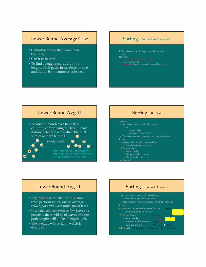
Lower Bound Average Case

• Cannot be worse than worst caseΘ(n lg n)

• Can it be better?

• To find average case, add up the lengths of all paths in the decision tree, and divide by the number of leaves.

Lower Bound Avg. II

• Because all non-leaves have two children, compressing the tree to make it more balanced will reduce the total sum of all path lengths.

C

X

A B

Switch X and C

C

X

A B

Path from root to C increases by 1,Path from root to A&B decreases by 1,Net reduction of 1 in the total.

Lower Bound Avg. III

• Algorithms with balanced decision trees perform better, on the average than algorithms with unbalanced trees.

• In a balanced tree with as few leaves as possible, there will be n! leaves and the path lengths will all be of length lg n!.

• The average will be lg n!, which isΘ(n lg n)

Sorting - Better than O(n log n) ?

• If all we know about the keys is an ordering rule

– No!

• However,

– If we can compute an address from the key(in constant time) then bin sort algorithms can provide better performance

Sorting - Bin Sort

• Assume

– All the keys lie in a small, fixed range

» eg

• integers 0-99

• characters ‘A’-’z’, ‘0’-’9’

– There is at most one item with each value of the key

• Bin sort

Allocate a bin for each value of the key

» Usually an entry in an array

For each item,

» Extract the key

» Compute it’s bin number

» Place it in the bin

Finished!

Sorting - Bin Sort: Analysis


» There are m possible key values


• Bin sort

Allocate a bin for each value of the key O(m)


For each item, n times

» Extract the key O(1)

» Compute it’s bin number O(1)

» Place it in the bin O(1) x n O(n)

Finished! O(n) + O(m) = O(n+m) = O(n) if n >> m

Key condition

Sorting - Bin Sort: Caveat

• Key Range


» There are m possible key values

– If this condition is not met, eg m >> n,

then bin sort is O(m) • Example

– Key is a 32-bit integer, m = 232

– Clearly, this isn’t a good way to sort a few thousand integers

– Also, we may not have enough space for bins!

• Bin sort trades space for speed!

– There’s no free lunch!

Sorting - Bin Sort with duplicates


• Bin sort

Allocate a bin for each value of the key O(m)


» Array of list heads

For each item, n times

» Extract the key O(1)

» Compute it’s bin number O(1)

» Add it to a list O(1) x n O(n)

» Join the lists O(m)

» Finished! O(n) + O(m) = O(n+m) = O(n) if n >> m

Relax?

Bucket Sort

• Bucket sort– Assumption: the keys are in the range [0, N)

– Basic idea: 1. Create N linked lists (buckets) to divide interval [0,N) into subintervals of size 1

2. Add each input element to appropriate bucket

3. Concatenate the buckets

– Expected total time is O(n + N), with n = size of original sequence» if N is O(n) sorting algorithm in O(n) !

Bucket Sort

Each element of the array is put in one of the N “buckets”

Bucket Sort

Now, pull the elements from

the buckets into the array

At last, the sorted array

(sorted in a stable way):

Does it Work for Real Numbers?

•What if keys are not integers?

– Assumption: input is n reals from [0, 1)

– Basic idea:

» Create N linked lists (buckets) to divide interval [0,1) into subintervals of size 1/N

» Add each input element to appropriate bucket and sort buckets with insertion sort

– Uniform input distribution O(1) bucket size

» Therefore the expected total time is O(n)

– Distribution of keys in buckets similar with …. ?

79

Non-Comparison Sort – Counting Sort

• Assumption: n input numbers are integers in the

range [0,k], k=O(n).

• Idea:

– Determine the number of elements less than x, for each input x.

– Place x directly in its position.

80

Counting Sort - pseudocode

Counting-Sort(A,B,k)

• for i←0 to k

• do C[i] ←0

• for j←1 to length[A]

• do C[A[j]] ←C[A[j]]+1

• // C[i] contains number of elements equal to i.

• for i←1 to k

• do C[i]=C[i]+C[i-1]

• // C[i] contains number of elements ≤ i.

• for j←length[A] downto 1

• do B[C[A[j]]] ←A[j]

• C[A[j]] ←C[A[j]]-1

81

Counting Sort - example

82

Counting Sort - analysis

1. for i←0 to k Θ(k)

2. do C[i] ←0 Θ(1)

3. for j←1 to length[A] Θ(n)

4. do C[A[j]] ←C[A[j]]+1 Θ(1) (Θ(1) Θ(n)= Θ(n))

5. // C[i] contains number of elements equal to i. Θ(0)

6. for i←1 to k Θ(k)

7. do C[i]=C[i]+C[i-1] Θ(1) (Θ(1) Θ(n)= Θ(n))

8. // C[i] contains number of elements ≤ i. Θ(0)

9. for j←length[A] downto 1 Θ(n)

10. do B[C[A[j]]] ←A[j] Θ(1) (Θ(1) Θ(n)= Θ(n))

11. C[A[j]] ←C[A[j]]-1 Θ(1) (Θ(1) Θ(n)= Θ(n))

Total cost is Θ(k+n), suppose k=O(n), then total cost is Θ(n).

So, it beats the ΩΩΩΩ(n log n) lower bound!

83

Stable sort

• Preserves order of elements with the same key.

• Counting sort is stable.

Crucial question: can counting sort be used to

sort large integers efficiently?

84

Radix sort

Radix-Sort(A,d)

• for i←1 to d

• do use a stable sort to sort A on digit i

Analysis:

Given n d-digit numbers where each digit takes on up to k values, Radix-Sort sorts these numbers

correctly in Θ(d(n+k)) time.

85

Radix sort - example

1019

3075

2225

2231

2231307522251019

1019222522313075

1019307522252231

Sorted!

101922312225 3075

1019222522313075

1019307522312225

Not sorted!

Introduction to Algorithms

Chapter 9: Median and Order Statistics.

87

Selection

• General Selection Problem:

– select the i-th smallest element form a set of n distinct

numbers

– that element is larger than exactly i - 1 other elements

• The selection problem can be solved in O(nlgn) time

– Sort the numbers using an O(nlgn)-time algorithm, such as

merge sort

– Then return the i-th element in the sorted array

88

Medians and Order Statistics

Def.: The i-th order statisticorder statisticorder statisticorder statistic of a set of n elements is the i-th smallest

element.

• The minimum of a set of elements:

– The first order statistic i = 1

• The maximum of a set of elements:

– The n-th order statistic i = n

• The median is the “halfway point” of the set

– i = (n+1)/2, is unique when n is odd

– i = (n+1)/2 = n/2 (lower median) and (n+1)/2 = n/2+1 (upper

median), when n is even

89

Finding Minimum or Maximum

Alg.:MINIMUM(A, n)min ← A[1]for i← 2 to n

do if min > A[i]then min ← A[i]

return min

• How many comparisons are needed?

– n – 1: each element, except the minimum, must be compared to a

smaller element at least once

– The same number of comparisons are needed to find the

maximum

– The algorithm is optimal with respect to the number of comparisons performed

90

Simultaneous Min, Max

• Find min and max independently

– Use n – 1 comparisons for each ⇒ total of 2n – 2

• At most 3n/2 comparisons are needed

– Process elements in pairs

– Maintain the minimum and maximum of elements seen so far

– Don’t compare each element to the minimum and maximum

separately

– Compare the elements of a pair to each other

– Compare the larger element to the maximum so far, and

compare the smaller element to the minimum so far

– This leads to only 3 comparisons for every 2 elements

91

Analysis of Simultaneous Min, Max

• Setting up initial values:

– n is odd:

– n is even:

• Total number of comparisons:

– n is odd: we do 3(n-1)/2 comparisons

– n is even: we do 1 initial comparison + 3(n-2)/2 more

comparisons = 3n/2 - 2 comparisons

set both min and max to the first element

compare the first two elements, assign the smallest one to min and the largest one to max

92

Example: Simultaneous Min, Max

• n = 5 (odd), array A = 2, 7, 1, 3, 4

1. Set min = max = 2

2. Compare elements in pairs:

– 1 < 7 ⇒ compare 1 with min and 7 with max

⇒ min = 1, max = 7


⇒ min = 1, max = 7

We performed: 3(n-1)/2 = 6 comparisons

3 comparisons

3 comparisons

93

Example: Simultaneous Min, Max

• n = 6 (even), array A = 2, 5, 3, 7, 1, 4

1. Compare 2 with 5: 2 < 5

2. Set min = 2, max = 5

3. Compare elements in pairs:


⇒ min = 2, max = 7


⇒ min = 1, max = 7

We performed: 3n/2 - 2 = 7 comparisons

3 comparisons

3 comparisons

1 comparison

9

Medians and Order Statistics

CLRS Chapter 9

upper median

3 4 13 14 23 27 41

lower median

54 65 75

The lower median is the -th order statistic

The upper median is the -th order statistic

If n is odd, lower and upper median are the same

What Are Order Statistics?

8th order statistic

3 4 13 14 23 27 41 54 65 75

The k-th order statistic is the k-th smallest element of an array.

2

n

2

n

9

What are Order Statistics?

Selecting ith-ranked item from a collection.

– First: i = 1

– Last: i = n

– Median(s): i =

2

n,

2

n

9

Order Statistics Overview

• Assume collection is unordered, otherwise trivial.

find ith order stat = A[i]

• Can sort first – Θ(n lg n), but can do better – Θ(n).

• I can find max and min in Θ(n) time (obvious)

9

Order Statistics Overview

How can we modify Quicksort to obtain

expected-case Θ(n)?

?

?

Pivot, partition, but recur only on one set of data. No join.

9

Using the Pivot Idea

• Randomized-Select(A[p..r],i) looking for ith o.s.

if p = rreturn A[p]

q <- Randomized-Partition(A,p,r)

k <- q-p+1 the size of the left partition

if i=k then the pivot value is the answer

return A[q]

else if i < k then the answer is in the front

return Randomized-Select(A,p,q-1,i)

1

Randomized Selection

• Analyzing RandomizedSelect()

– Worst case: partition always 0:n-1

T(n) = T(n-1) + O(n)

= O(n2)

» No better than sorting!

– “Best” case: suppose a 9:1 partition

T(n) = T(9n/10) + O(n)

= O(n) (Master Theorem, case 3)

» Better than sorting!

– Average case: O(n) remember from quicksort

1

Worst-Case Linear-Time Selection

• Randomized algorithm works well in practice

• What follows is a worst-case linear time algorithm, really of theoretical interest only

• Basic idea:

– Guarantee a good partitioning element

– Guarantee worst-case linear time selection

•Warning: Non-obvious & unintuitive algorithm ahead!

1

Worst-Case Linear-Time Selection

• The algorithm in words:1. Divide n elements into groups of 5

2. Find median of each group (How? How long?)

3. Use Select() recursively to find median x of the n/5medians

4. Partition the n elements around x. Let k = rank(x)

5. if (i == k) then return x

if (i < k) then use Select() recursively to find ith smallest element in first partitionelse (i > k) use Select() recursively to find (i-k)th smallest

element in last partition

1

Order Statistics: Algorithm

Select(A,n,i):Divide input into groups of size 5.

/* Partition on median-of-medians */

medians = array of each group’s median.

pivot = Select(medians, , )

Left Array L and Right Array G = partition(A, pivot)

/* Find ith element in L, pivot, or G */

k = |L| + 1

If i=k, return pivot

If i<k, return Select(L, k-1, i)

If i>k, return Select(G, n-k, i-k)

O(n)

T(n)

O(n)

T( )

O(n)

O(1)

O(1)

T(k)

T(n-k)

Only one

done.

All this

to find agood split.

n/5

n/5 n/5 n/10

1

Order Statistics: Analysis

( ) ( )( ) O(n)k-n1,-kmaxT5

nTnT ++

=

#less #greater

How to simplify?

1


One group of 5 elements.

Median

Greater

Elements

Lesser

Elements

1


All groups of 5 elements.(And at most one smaller group.)

Median of

Medians

Greater

Medians

Lesser

Medians

1


Definitely Lesser

Elements

Definitely Greater

Elements

1

Order Statistics: Analysis 1

Must recur on all elements outside one of these boxes.

How many?

1

Order Statistics: Analysis 1

At most 610

7n2

5

n22

5

n5 +≤

+

25n full groups of 5 partial groups of 2 25n

Count elements

outside smaller box.

1


A very unusual recurrence. How to solve?

( ) ( )nO610

7nT

5

nTnT +

++

=

??

1


Substitution: Prove .

( ) nd610

7nc

5

ncnT ×+

+×+

×≤

( ) ncnT ×≤

nc ×≤

nd7c10nc0 ×−−×≤when choose c,d such that

nd610

7nc1

5

nc ×+

+×+

+×≤ Overestimate ceiling

nd7cnc10

9×++×= Algebra

( )nd7c10ncnc ×−−×−×= Algebra

1

Order Statistics

Why groups of 5?

Sum of two recurrence sizes must be < 1.

Grouping by 5 is smallest size that works.

? ?

113

General Selection Problem

• Select the i-th order statistic (i-th smallest element) form a set of n distinct numbers

• Idea:– Partition the input array similarly with the approach used for Quicksort (use RANDOMIZED-PARTITION)

– Recurse on one side of the partition to look for the i-thelement depending on where i is with respect to the pivot

• Selection of the i-th smallest element of the array A can be done in Θ(n) time

qp r

i < k ⇒ search in this partition

i > k ⇒ search in this partition

A

114

Randomized Select

Alg.: RANDOMIZED-SELECT(A, p, r, i )

if p = r

then return A[p]

q←RANDOMIZED-PARTITION(A, p, r)

k ← q - p + 1

if i = k pivot value is the answer

then return A[q]

elseif i < k

then return RANDOMIZED-SELECT(A, p, q-1, i )

else return RANDOMIZED-SELECT(A, q + 1, r, i-k)

• Try: A=1,4,2,6,8,5

qp r

i < k ⇒ search in this partition

i > k ⇒ search in this partition

q-1 q+1

pivot

115

Analysis of Running Time

• Worst case running time:

– If we always partition around the largest/smallest remaining

element

– Partition takes Θ(n) time

– T(n) = O(1) (choose the pivot) + Θ(n) (partition) + T(n-1)

= 1 + n + T(n-1) = Θ(n2)

q

p r

n-1 elements

Θ(n2)

116

A Better Selection Algorithm

• Can perform Selection in O(n)Worst Case

• Idea: guarantee a good split on partitioning

– Running time is influenced by how “balanced” are the

resulting partitions

• Use a modified version of PARTITION

– Takes as input the element around which to partition

Selection in O(n)Worst Case

1. Divide the n elements into groups of 5 ⇒ n/5 groups 2. Find the median of each of the n/5 groups

• Use insertion sort, then pick the median3. Use SELECT recursively to find the median x of the n/5medians4. Partition the input array around x, using the modified version of

PARTITION

• There are k-1 elements on the low side of the partition and n-k on the high side

5. If i = k then return x. Otherwise, use SELECT recursively:

• Find the i-th smallest element on the low side if i < k• Find the (i-k)-th smallest element on the high side if i > k

A: x1 x2 x3 xn/5

xxk – 1 elements n - k elements

118

Example

• Find the –11th smallest element in array:A = 12, 34, 0, 3, 22, 4, 17, 32, 3, 28, 43, 82, 25, 27, 34, 2 ,19 ,12 ,5 ,18 ,20 ,33, 16, 33, 21, 30, 3, 47

1. Divide the array into groups of 5 elements

41732328

12340322

4382252734

21912518

2033163321

30347

119

Example (cont.)

2. Sort the groups and find their medians

3. Find the median of the medians

12, 12, 17, 21, 34, 30

43173228

03123422

2527344382

25121918

2016213333

33047

120

Example (cont.)

4. Partition the array around the median of medians (17)

First partition:

12, 0, 3, 4, 3, 2, 12, 5, 16, 3

Pivot:

17 (position of the pivot is q = 11)

Second partition:

34, 22, 32, 28, 43, 82, 25, 27, 34, 19, 18, 20, 33, 33, 21, 30, 47

To find the 6-th smallest element we would have to recurse our search in the first partition.

The End

Sorting - Generalised Bin Sort

• Radix sort

– Bin sort in phases

– Example

– Phase 1 - Sort by least significant digit

36 9 0 25 1 49 64 16 81 4

0 1 2 3 4 5 6 7 8 9

0 1

81

64

4

25 36

16

9

49


• Radix sort - Bin sort in phases


– Phase 2 - Sort by most significant digit

0 1 2 3 4 5 6 7 8 9

0 1

81

64

4

25 36

16

9

49

0 1 2 3 4 5 6 7 8 9

0





0 1 2 3 4 5 6 7 8 9

0 1

81

64

4

25 36

16

9

49

0 1 2 3 4 5 6 7 8 9

0

1

Be careful to

add after anythingin the bin already!





0 1 2 3 4 5 6 7 8 9

0 1

81

64

4

25 36

16

9

49

0 1 2 3 4 5 6 7 8 9

0

1

81





0 1 2 3 4 5 6 7 8 9

0 1

81

64

4

25 36

16

9

49

0 1 2 3 4 5 6 7 8 9

0

1

8164





0 1 2 3 4 5 6 7 8 9

0 1

81

64

4

25 36

16

9

49

0 1 2 3 4 5 6 7 8 9

0

1

4

8164

1 2 3 4 5 6 7 8 9

816425 3616 49





0 1 2 3 4 5 6 7 8 9

0 1

81

64

4

25 36

16

9

49

0

0

1

4

9

Note that the 0

bin had to bequite large!

1 2 3 4 5 6 7 8 9

816425 3616 49





0 1 2 3 4 5 6 7 8 9

0 1

81

64

4

25 36

16

9

49

0

0

1

4

9

How much

space is neededin each phase?

n items

m bins


• Radix sort - Analysis


» Create m bins O(m)

» Allocate n items O(n)

– Phase 2

» Create m bins O(m)

» Allocate n items O(n)

– Final

» Link m bins O(m)

– All steps in sequence, so add

– Total O(3m+2n) O(m+n) O(n) for m<<n

Radix Sort

• Start with least significant digit

• Separate keys into groups based on value of current digit

• Make sure not to disturb original order of keys

• Combine separate groups in ascending order

• Repeat, scanning digits in reverse order

Radix Sort: Example

0 0 00 0 1

0 1 00 1 1

1 0 01 0 11 1 0

1 1 1

0 0 0

0 0 1

0 1 0

0 1 1

1 0 0

1 0 1

1 1 0

1 1 1

0 0 0

0 0 1

0 1 0

0 1 1

1 0 0

1 0 1

1 1 0

1 1 1

0 0 0

0 0 1

0 1 0

0 1 1

1 0 0

1 0 1

1 1 0

1 1 1

0 0 0

0 0 10 1 0

0 1 1

1 0 0

1 0 1

1 1 0

1 1 1

0 0 00 0 10 1 00 1 1

1 0 01 0 11 1 01 1 1

Radix Sort: Analysis

• Each digit requires n comparisons

• The algorithm is Θ(n)

• The preceding lower bound analysis does not apply, because Radix Sort does not compare keys.

• Radix Sort is sometimes known as bucket sort. (Any distinction between the two is unimportant

• Alg. was used by operators of card sorters.

Documents

Paper folding myth Repeated Minimum: Code