1

Paper 1323-2017

Real AdaBoost: boosting for credit scorecards and similarity to WOE logistic regression

Paul K. Edwards, Dina Duhon, Suhail Shergill

Scotiabank

ABSTRACT

Adaboost is a machine learning algorithm that builds a series of small decision trees, adapting each tree to predict difficult cases missed by the previous trees and combining all trees into a single model. We will discuss the AdaBoost methodology and introduce the extension called Real AdaBoost. Real AdaBoost comes from a strong academic pedigree: its authors are pioneers of machine learning and the method has well-established empirical and theoretical support spanning 15 years. Practically speaking, Real AdaBoost is able to produce readable credit scorecards and offers attractive features including variable interaction and adaptive, stage-wise binning. We will contrast Real AdaBoost to the dominant methodology for creating credit scorecards: stepwise weight of evidence logistic regression (SWOELR). Real AdaBoost is remarkably similar to SWOELR and is well positioned to serve as a benchmark for SWOELR models; it may even offer a statistical framework by which we can understand the power of SWOELR. We offer a macro to generate Real AdaBoost models in SAS.

INTRODUCTION

Financial institutions (FIs) must develop a wide range of models for marketing, fraud detection, loan adjudication, etc. Modeling has undergone a recent renaissance as machine learning has exploded – spurned by the availability of advanced statistical techniques, the ubiquity of powerful computers to execute these techniques, and the well-publicized successes of the companies who have embraced these methods (Parloff 2016). Modeling departments within some FIs face opposing demands: executives want some of the famed value of advanced methods, while government regulators, internal deployment teams and front-line staff want models that are easy to implement, interpret and understand. In this paper we review Real AdaBoost, a machine learning technique that may offer a middle-ground between powerful, but opaque machine learning methods and transparent conventional methods.

CONSUMER RISK MODELS

One field of modeling where FIs must often strike a balance between power and transparency is consumer risk modeling. Consumer risk modeling involves ranking customers by their credit worthiness (the likelihood they will repay a loan): first by identifying customer characteristics that indicate risk of delinquency, and then combining them mathematically to calculate a relative risk score for each customer (common characteristics include: past loan delinquency, high credit utilization, etc.).

CREDIT SCORECARDS

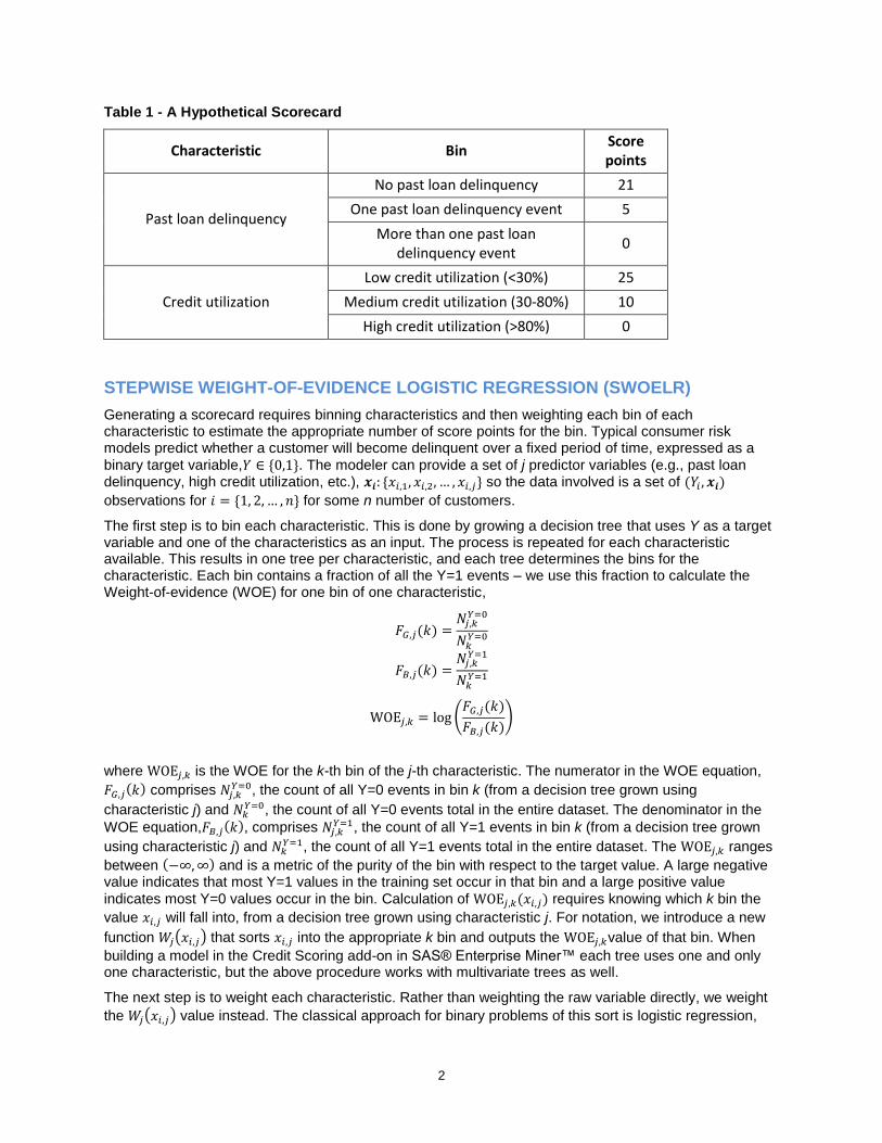
In order to keep the consumer risk models as transparent as possible, many FIs require that the final output of the model be in the form of a scorecard (an example is shown in Table 1). Credit scorecards are a popular way to represent customer risk models due to their simplicity, readability, and the ease with which business expertise can be incorporated during the modeling process (Maldonado et al. 2013).

A scorecard lists a number of characteristics that indicate risk and each characteristic is subdivided into a small number of bins defined by ranges of values for that characteristic (e.g., credit utilization: 30-80% is a bin for the credit utilization characteristic). Each bin is assigned a number of score points, a value derived from a statistical model and proportional to the risk of that bin (SAS 2012). A customer will fall into one and only one bin per characteristic and the final score of the applicant is the sum of the points assigned by each bin (plus an intercept). This final score is proportional to consumer risk. The procedure for developing scorecards is termed stepwise weight of evidence logistic regression (SWOELR) and is implemented in the Credit Scoring add-on in SAS® Enterprise Miner™.

2

Table 1 - A Hypothetical Scorecard

Characteristic Bin Score points

Past loan delinquency

No past loan delinquency 21

One past loan delinquency event 5

More than one past loan delinquency event

0

Credit utilization

Low credit utilization (<30%) 25

Medium credit utilization (30-80%) 10

High credit utilization (>80%) 0

STEPWISE WEIGHT-OF-EVIDENCE LOGISTIC REGRESSION (SWOELR)

Generating a scorecard requires binning characteristics and then weighting each bin of each characteristic to estimate the appropriate number of score points for the bin. Typical consumer risk models predict whether a customer will become delinquent over a fixed period of time, expressed as a

binary target variable,𝑌 ∈ {0,1}. The modeler can provide a set of j predictor variables (e.g., past loan delinquency, high credit utilization, etc.), 𝒙𝒊: {𝑥𝑖,1, 𝑥𝑖,2, … , 𝑥𝑖,𝑗} so the data involved is a set of (𝑌𝑖 , 𝒙𝒊)

observations for 𝑖 = {1, 2, … , 𝑛} for some n number of customers.

The first step is to bin each characteristic. This is done by growing a decision tree that uses Y as a target variable and one of the characteristics as an input. The process is repeated for each characteristic available. This results in one tree per characteristic, and each tree determines the bins for the characteristic. Each bin contains a fraction of all the Y=1 events – we use this fraction to calculate the Weight-of-evidence (WOE) for one bin of one characteristic,

𝐹𝐺,𝑗(𝑘) =𝑁𝑗,𝑘

𝑌=0

𝑁𝑘𝑌=0

𝐹𝐵,𝑗(𝑘) =𝑁𝑗,𝑘

𝑌=1

𝑁𝑘𝑌=1

WOE𝑗,𝑘 = log (𝐹𝐺,𝑗(𝑘)

𝐹𝐵,𝑗(𝑘))

where WOE𝑗,𝑘 is the WOE for the k-th bin of the j-th characteristic. The numerator in the WOE equation,

𝐹𝐺,𝑗(𝑘) comprises 𝑁𝑗,𝑘𝑌=0, the count of all Y=0 events in bin k (from a decision tree grown using

characteristic j) and 𝑁𝑘𝑌=0, the count of all Y=0 events total in the entire dataset. The denominator in the

WOE equation,𝐹𝐵,𝑗(𝑘), comprises 𝑁𝑗,𝑘𝑌=1, the count of all Y=1 events in bin k (from a decision tree grown

using characteristic j) and 𝑁𝑘𝑌=1, the count of all Y=1 events total in the entire dataset. The WOE𝑗,𝑘 ranges

between (−∞, ∞) and is a metric of the purity of the bin with respect to the target value. A large negative value indicates that most Y=1 values in the training set occur in that bin and a large positive value

indicates most Y=0 values occur in the bin. Calculation of WOE𝑗,𝑘(𝑥𝑖,𝑗) requires knowing which k bin the

value 𝑥𝑖,𝑗 will fall into, from a decision tree grown using characteristic j. For notation, we introduce a new

function 𝑊𝑗(𝑥𝑖,𝑗) that sorts 𝑥𝑖,𝑗 into the appropriate k bin and outputs the WOE𝑗,𝑘value of that bin. When

building a model in the Credit Scoring add-on in SAS® Enterprise Miner™ each tree uses one and only one characteristic, but the above procedure works with multivariate trees as well.

The next step is to weight each characteristic. Rather than weighting the raw variable directly, we weight

the 𝑊𝑗(𝑥𝑖,𝑗) value instead. The classical approach for binary problems of this sort is logistic regression,

3

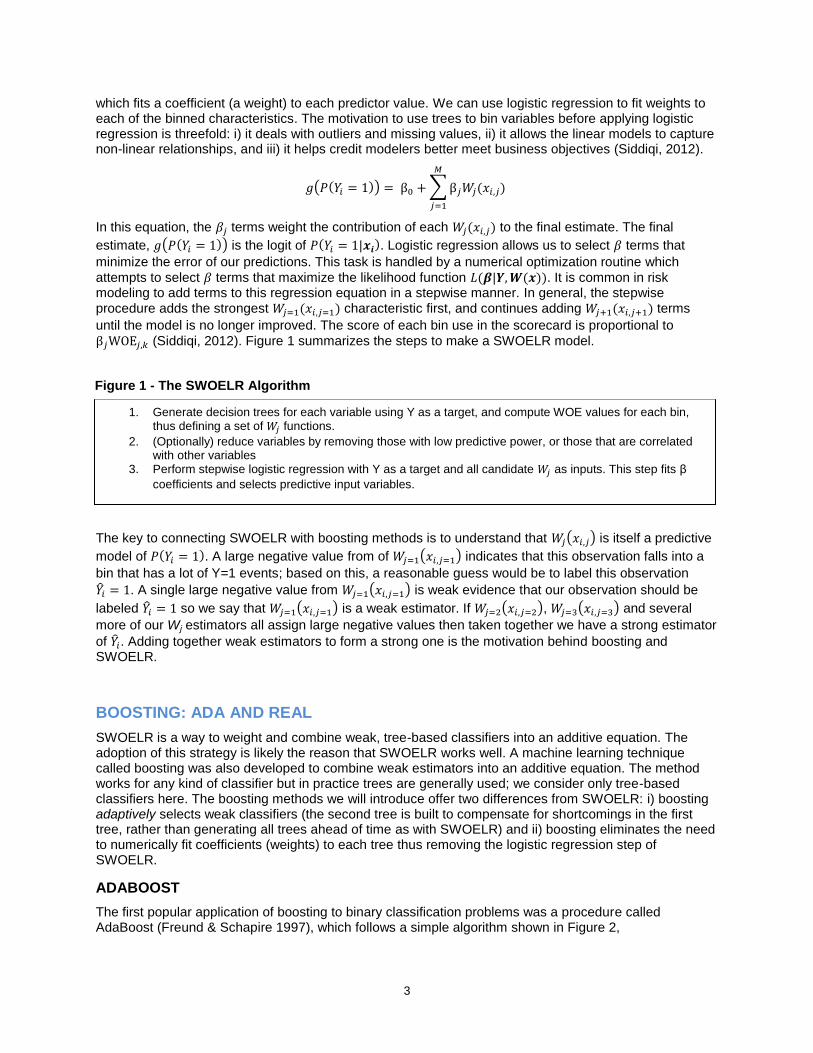
which fits a coefficient (a weight) to each predictor value. We can use logistic regression to fit weights to each of the binned characteristics. The motivation to use trees to bin variables before applying logistic regression is threefold: i) it deals with outliers and missing values, ii) it allows the linear models to capture non-linear relationships, and iii) it helps credit modelers better meet business objectives (Siddiqi, 2012).

𝑔(𝑃(𝑌𝑖 = 1)) = β0 + ∑ β𝑗𝑊𝑗(𝑥𝑖,𝑗)

𝑀

𝑗=1

In this equation, the 𝛽𝑗 terms weight the contribution of each 𝑊𝑗(𝑥𝑖,𝑗) to the final estimate. The final

estimate, 𝑔(𝑃(𝑌𝑖 = 1)) is the logit of 𝑃(𝑌𝑖 = 1|𝒙𝒊). Logistic regression allows us to select 𝛽 terms that

minimize the error of our predictions. This task is handled by a numerical optimization routine which

attempts to select 𝛽 terms that maximize the likelihood function 𝐿(𝜷|𝒀, 𝑾(𝒙)). It is common in risk modeling to add terms to this regression equation in a stepwise manner. In general, the stepwise procedure adds the strongest 𝑊𝑗=1(𝑥𝑖,𝑗=1) characteristic first, and continues adding 𝑊𝑗+1(𝑥𝑖,𝑗+1) terms

until the model is no longer improved. The score of each bin use in the scorecard is proportional to

β𝑗WOE𝑗,𝑘 (Siddiqi, 2012). Figure 1 summarizes the steps to make a SWOELR model.

The key to connecting SWOELR with boosting methods is to understand that 𝑊𝑗(𝑥𝑖,𝑗) is itself a predictive

model of 𝑃(𝑌𝑖 = 1). A large negative value from of 𝑊𝑗=1(𝑥𝑖,𝑗=1) indicates that this observation falls into a

bin that has a lot of Y=1 events; based on this, a reasonable guess would be to label this observation

�̂�𝑖 = 1. A single large negative value from 𝑊𝑗=1(𝑥𝑖,𝑗=1) is weak evidence that our observation should be

labeled �̂�𝑖 = 1 so we say that 𝑊𝑗=1(𝑥𝑖,𝑗=1) is a weak estimator. If 𝑊𝑗=2(𝑥𝑖,𝑗=2), 𝑊𝑗=3(𝑥𝑖,𝑗=3) and several

more of our Wj estimators all assign large negative values then taken together we have a strong estimator

of �̂�𝑖. Adding together weak estimators to form a strong one is the motivation behind boosting and SWOELR.

BOOSTING: ADA AND REAL

SWOELR is a way to weight and combine weak, tree-based classifiers into an additive equation. The adoption of this strategy is likely the reason that SWOELR works well. A machine learning technique called boosting was also developed to combine weak estimators into an additive equation. The method works for any kind of classifier but in practice trees are generally used; we consider only tree-based classifiers here. The boosting methods we will introduce offer two differences from SWOELR: i) boosting adaptively selects weak classifiers (the second tree is built to compensate for shortcomings in the first tree, rather than generating all trees ahead of time as with SWOELR) and ii) boosting eliminates the need to numerically fit coefficients (weights) to each tree thus removing the logistic regression step of SWOELR.

ADABOOST

The first popular application of boosting to binary classification problems was a procedure called AdaBoost (Freund & Schapire 1997), which follows a simple algorithm shown in Figure 2,

1. Generate decision trees for each variable using Y as a target, and compute WOE values for each bin, thus defining a set of 𝑊𝑗 functions.

2. (Optionally) reduce variables by removing those with low predictive power, or those that are correlated with other variables

3. Perform stepwise logistic regression with Y as a target and all candidate 𝑊𝑗 as inputs. This step fits β

coefficients and selects predictive input variables.

Figure 1 - The SWOELR Algorithm

4

The concept is very similar to SWOELR: AdaBoost constructs an equation, 𝑓(𝒙𝒊), which adds up a series of weak classifiers, ℎ𝑗, each weighted by 𝛼𝑗,

𝐺(𝑃(𝑌𝑖 = 1)) = 𝑓(𝒙𝒊) = ∑ 𝛼𝑗ℎ𝑗(𝒙𝒊)

𝑀

𝑗=1

Just like SWOELR, the classifiers are trees which transform their input: ℎ𝑗(𝒙𝒊), like 𝑊𝑗(𝑥𝑖,𝑗) first assigns a

bin using a decision tree. Instead of returning the WOE, which is proportional to the number of Y=1

events in the bin, the ℎ𝑗(𝒙𝒊) function returns a 1 or a 0, depending on the most common event in the bin.

Instead of a prediction in the range (−∞, ∞) like WOE, each ℎ𝑗 simply returns a binary label for each Y

indicating the most likely label. In contrast to SWOELR, the coefficient 𝛼𝑗 does not have to be estimated

numerically, but is calculated analytically using the error on ℎ𝑗. Similar to the stepwise procedure used by

SWOELR, AdaBoost terms are added sequentially up to (a user-defined) M terms. The final estimate

𝐺(𝑃(𝑌𝑖 = 1)) ∈ (−∞, ∞) is proportional to risk and can be scaled to the domain [0,1] with

logit−1 (𝐺(𝑃(𝑌𝑖 = 1))).

The AdaBoost procedure is an established machine learning algorithm and has undergone intense theoretical and empirical testing and has guaranteed bounds of error (Schapire 2003). Even still,

researchers studied whether the ℎ𝑗 classifier could be made to return a continuous prediction (like WOE)

rather than a binary one and if the 𝛼𝑗 coefficient could be done away with completely.

REAL ADABOOST

Following the publication of the AdaBoost procedure, Friedman, Hastie, and Tibshirani (2000) analyzed the procedure through a formal statistical lens. They also offered a modification of the AdaBoost procedure which they called Real AdaBoost. They proved that Real AdaBoost (and AdaBoost) asymptotically fits an additive logistic regression meaning that Real AdaBoost attains the same goal as SWOELR: a relaxed, non-linear version of logistic regression. Real AdaBoost also extends AdaBoost with

a real-valued classifier, 𝐻𝑗 =1

2𝑙𝑜𝑔 (

𝑃𝑤(𝑌=1|𝑥)

𝑃𝑤(𝑌=0|𝑥)), or one-half the weighted log-odds predicted by the classifier.

This classifier bears a striking similarity to the proportional odds used in the WOE equation as part of the

𝑊𝑗 function in SWOELR. Friedman and co-authors show that adopting Real AdaBoost removes the need

for a coefficient as the optimal coefficient is always 𝛼𝑗 = 1. Their empirical results suggest that Real

AdaBoost can reach a strong classifier with fewer trees than AdaBoost.

The final equation of Real AdaBoost is,

𝐺(𝑃(𝑌𝑖 = 1)) = 𝐹(𝑥𝑖 ) = ∑ 𝐻𝑗(𝑥𝑖)

𝑀

𝑗=1

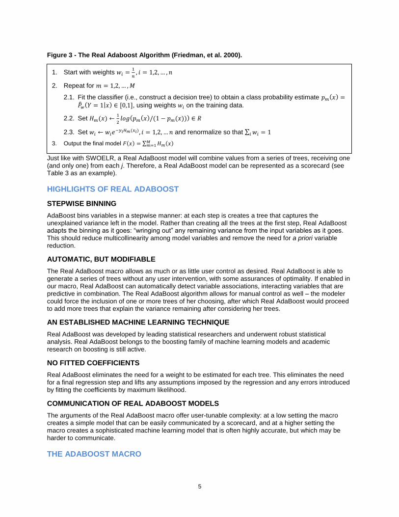
and the full Real AdaBoost algorithm is shown in Figure 3.

1. Set initial weights: 𝑤1, 𝑤2, … , 𝑤𝑛 = 1/𝑛 2. Find the weak classifier ℎ𝑡(𝑥) (i.e., construct a decision tree) that minimizes the weighted

misclassification error. This step tries harder to correctly classify observations with high weights. 3. Add ℎ𝑡(𝑥) to the final model ensemble.

4. Update the weights, increasing the weight of observations that the final model ensemble misclassifies. 5. Return to step 2.

Figure 2 - The Adaboost algorithm

5

Just like with SWOELR, a Real AdaBoost model will combine values from a series of trees, receiving one (and only one) from each j. Therefore, a Real AdaBoost model can be represented as a scorecard (see Table 3 as an example).

HIGHLIGHTS OF REAL ADABOOST

STEPWISE BINNING

AdaBoost bins variables in a stepwise manner: at each step is creates a tree that captures the unexplained variance left in the model. Rather than creating all the trees at the first step, Real AdaBoost adapts the binning as it goes: “wringing out” any remaining variance from the input variables as it goes. This should reduce multicollinearity among model variables and remove the need for a priori variable reduction.

AUTOMATIC, BUT MODIFIABLE

The Real AdaBoost macro allows as much or as little user control as desired. Real AdaBoost is able to generate a series of trees without any user intervention, with some assurances of optimality. If enabled in our macro, Real AdaBoost can automatically detect variable associations, interacting variables that are predictive in combination. The Real AdaBoost algorithm allows for manual control as well – the modeler could force the inclusion of one or more trees of her choosing, after which Real AdaBoost would proceed to add more trees that explain the variance remaining after considering her trees.

AN ESTABLISHED MACHINE LEARNING TECHNIQUE

Real AdaBoost was developed by leading statistical researchers and underwent robust statistical analysis. Real AdaBoost belongs to the boosting family of machine learning models and academic research on boosting is still active.

NO FITTED COEFFICIENTS

Real AdaBoost eliminates the need for a weight to be estimated for each tree. This eliminates the need for a final regression step and lifts any assumptions imposed by the regression and any errors introduced by fitting the coefficients by maximum likelihood.

COMMUNICATION OF REAL ADABOOST MODELS

The arguments of the Real AdaBoost macro offer user-tunable complexity: at a low setting the macro creates a simple model that can be easily communicated by a scorecard, and at a higher setting the macro creates a sophisticated machine learning model that is often highly accurate, but which may be harder to communicate.

THE ADABOOST MACRO

Figure 3 - The Real Adaboost Algorithm (Friedman, et al. 2000).

1. Start with weights 𝑤𝑖 =1

𝑛, 𝑖 = 1,2, … , 𝑛

2. Repeat for 𝑚 = 1,2, … , 𝑀

2.1. Fit the classifier (i.e., construct a decision tree) to obtain a class probability estimate 𝑝𝑚(𝑥) =�̂�𝑤(𝑌 = 1|𝑥) ∈ [0,1], using weights 𝑤𝑖 on the training data.

2.2. Set 𝐻𝑚(𝑥) ←1

2𝑙𝑜𝑔(𝑝𝑚(𝑥)/(1 − 𝑝𝑚(𝑥))) ∈ 𝑅

2.3. Set 𝑤𝑖 ← 𝑤𝑖𝑒−𝑦𝑖𝐻𝑚(𝑥𝑖), 𝑖 = 1,2, … 𝑛 and renormalize so that ∑ 𝑤𝑖 = 1𝑖

3. Output the final model 𝐹(𝑥) = ∑ 𝐻𝑚(𝑥)𝑀𝑚=1

6

This section explains the inputs and outputs of the Real AdaBoost macro. The most recent version of this code will always be available via Github

1.

REQUIREMENTS

Due to its reliance on the ARBOR procedure, the macro requires a license for SAS® Enterprise Miner™.

RUNNING THE MACRO

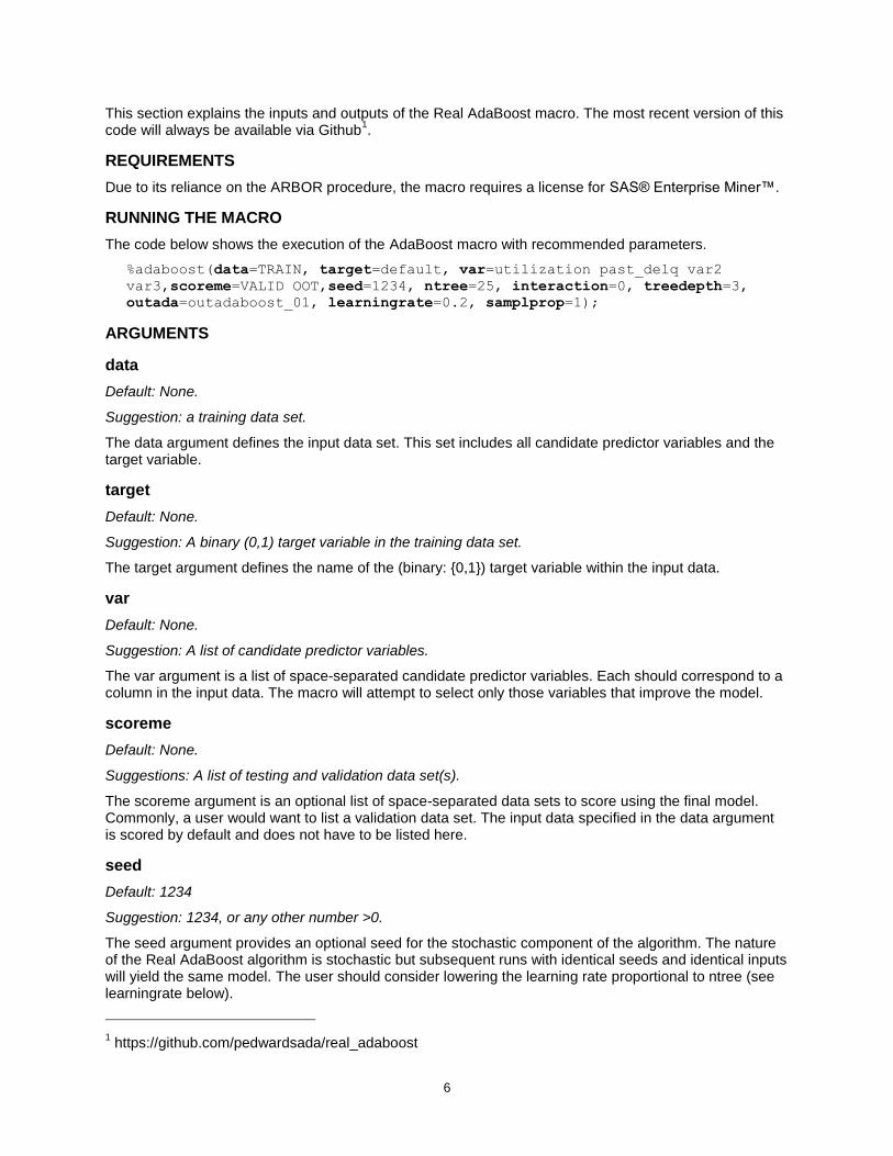
The code below shows the execution of the AdaBoost macro with recommended parameters.

%adaboost(data=TRAIN, target=default, var=utilization past_delq var2

var3,scoreme=VALID OOT,seed=1234, ntree=25, interaction=0, treedepth=3,

outada=outadaboost_01, learningrate=0.2, samplprop=1);

ARGUMENTS

data

Default: None.

Suggestion: a training data set.

The data argument defines the input data set. This set includes all candidate predictor variables and the target variable.

target

Default: None.

Suggestion: A binary (0,1) target variable in the training data set.

The target argument defines the name of the (binary: {0,1}) target variable within the input data.

var

Default: None.

Suggestion: A list of candidate predictor variables.

The var argument is a list of space-separated candidate predictor variables. Each should correspond to a column in the input data. The macro will attempt to select only those variables that improve the model.

scoreme

Default: None.

Suggestions: A list of testing and validation data set(s).

The scoreme argument is an optional list of space-separated data sets to score using the final model. Commonly, a user would want to list a validation data set. The input data specified in the data argument is scored by default and does not have to be listed here.

seed

Default: 1234

Suggestion: 1234, or any other number >0.

The seed argument provides an optional seed for the stochastic component of the algorithm. The nature of the Real AdaBoost algorithm is stochastic but subsequent runs with identical seeds and identical inputs will yield the same model. The user should consider lowering the learning rate proportional to ntree (see learningrate below).

1 https://github.com/pedwardsada/real_adaboost

7

ntree

Default: 25

Suggestion: A number 10-25.

The ntree argument specifies the number of trees to add together into a final model. A smaller number will yield a simpler model and a larger number (say, 25) will tend to yield a more predictive (but more complex) model.

treedepth

Default: 3

Suggestion: 2 or 3

The treedepth argument specifies the maximum depth of each tree. The maximum number of terminal nodes in each tree is thus 2

x. Boosting literature (Hastie et al. 2009 [pp. 363]) suggests that this number

should be small, like 2 or 3.

learningrate

Default: 0.2

Suggestion: High number (~1) when ntree is small, low number (0.1) when ntree is large.

The learningrate argument sets a coefficient to scale the contribution of each tree to the final model

score, 𝐹(𝑥𝑖 ) = ∑ 𝑐𝑓𝑗(𝑥𝑖)𝑀𝑗=1 , where 𝑐 ∈ (0,1] is the learning rate. The canonical Real AdaBoost uses

learningrate=1 but subsequent boosting literature recommends setting a value<1 (Hastie et al. 2009 [pp. 364–365]). In practice the user may find that a model built using a smaller value for learning rate may have low generalized error on a validation set, but may require many trees to attain this level of performance. Models with a higher learning rate will more “aggressively” fit a model so they may have good performance with a low number of at the expense of lower generalization.

interaction

Default: 1

Suggestion: 1 or 0.

The interaction argument toggles variable interaction within each tree. Setting a value of 1 means that each tree in the model may include splits based on any number of variables. A value of 0 forces each tree to include one and only one variable. Variables may be re-used in several trees. A value of 0 may result in a far simpler model that will be far easier to communicate – possibly at the expense of performance. Technically, the Real AdaBoost algorithm does not include any option like this so setting a value of 0 deviates from the published method.

outada

Default: outadaboost

Suggestion: outadaboost, or any named data set.

The outada argument sets the name of a new dataset that will be created to store the entire model. The dataset may be used later to score another data set using the macro adaboostscore.

samplprop

Default: 1

Suggestion: Generally 1, but for a large data set with E(Y)>>1%, try 0.5.

The sampleprop argument sets the proportion of the training population to “bag” (randomly subsample) at each iteration. With sampleprop<1, the j-th tree is built using only a fraction of full training set and the remaining 1-samplprop of the training is used to prune the tree. In general this should result in more

8

generalizable trees. Note that if the target is very sparse, (e.g., 𝐸(𝑌) <= 1%) setting sampleprop<1 may result in a worsened model as very few targets could be present in some bagged samples. Setting samplprop=1 disables this subsampling procedure entirely.

EXAMPLE

To demonstrate the macro usage and show sample outputs, we execute the macro on a synthetic data set created with the example code available on Github

2.

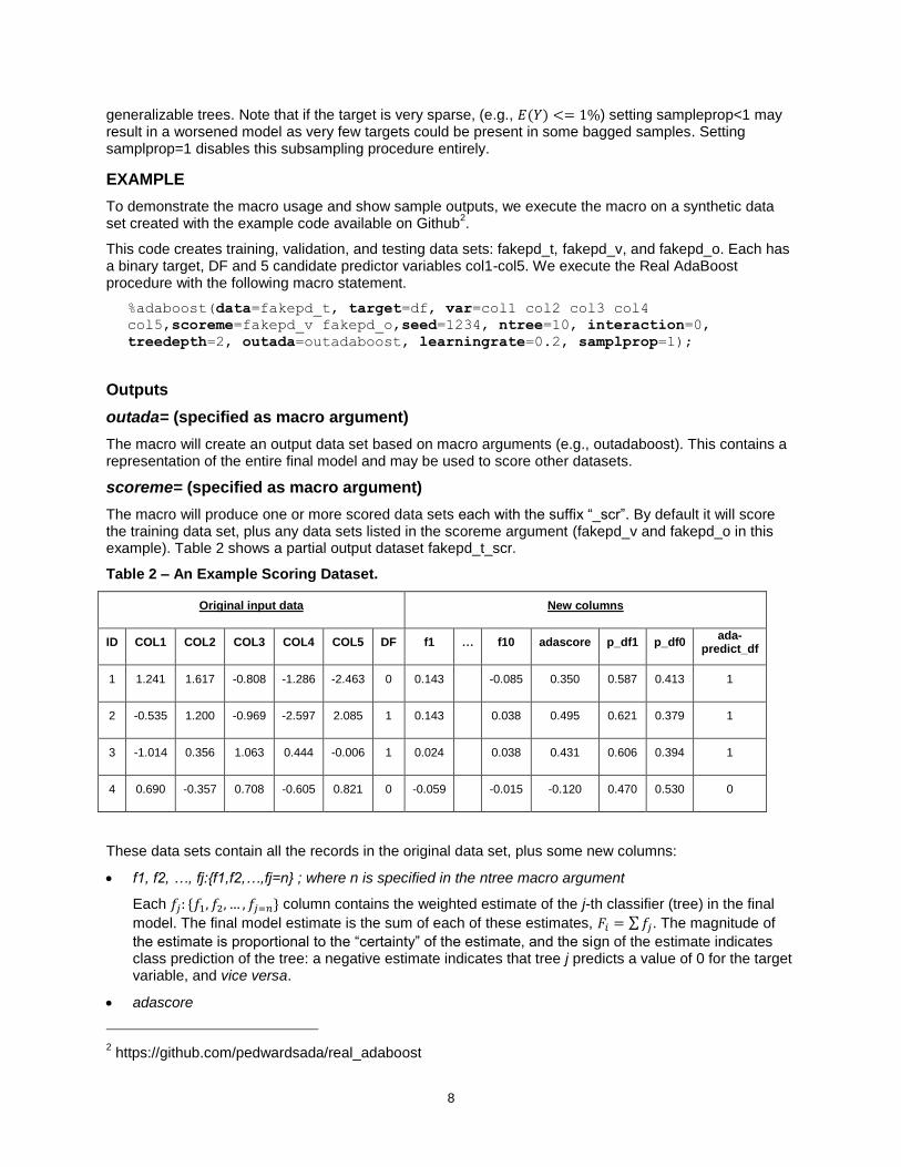
This code creates training, validation, and testing data sets: fakepd_t, fakepd_v, and fakepd_o. Each has a binary target, DF and 5 candidate predictor variables col1-col5. We execute the Real AdaBoost procedure with the following macro statement.

%adaboost(data=fakepd_t, target=df, var=col1 col2 col3 col4

col5,scoreme=fakepd_v fakepd_o,seed=1234, ntree=10, interaction=0,

treedepth=2, outada=outadaboost, learningrate=0.2, samplprop=1);

Outputs

outada= (specified as macro argument)

The macro will create an output data set based on macro arguments (e.g., outadaboost). This contains a representation of the entire final model and may be used to score other datasets.

scoreme= (specified as macro argument)

The macro will produce one or more scored data sets each with the suffix “_scr”. By default it will score the training data set, plus any data sets listed in the scoreme argument (fakepd_v and fakepd_o in this example). Table 2 shows a partial output dataset fakepd_t_scr.

Table 2 – An Example Scoring Dataset.

Original input data New columns

ID COL1 COL2 COL3 COL4 COL5 DF f1 … f10 adascore p_df1 p_df0 ada-

predict_df

1 1.241 1.617 -0.808 -1.286 -2.463 0 0.143 -0.085 0.350 0.587 0.413 1

2 -0.535 1.200 -0.969 -2.597 2.085 1 0.143 0.038 0.495 0.621 0.379 1

3 -1.014 0.356 1.063 0.444 -0.006 1 0.024 0.038 0.431 0.606 0.394 1

4 0.690 -0.357 0.708 -0.605 0.821 0 -0.059 -0.015 -0.120 0.470 0.530 0

These data sets contain all the records in the original data set, plus some new columns:

f1, f2, …, fj:{f1,f2,…,fj=n} ; where n is specified in the ntree macro argument

Each 𝑓𝑗: {𝑓1, 𝑓2, … , 𝑓𝑗=𝑛} column contains the weighted estimate of the j-th classifier (tree) in the final

model. The final model estimate is the sum of each of these estimates, 𝐹𝑖 = ∑ 𝑓𝑗. The magnitude of

the estimate is proportional to the “certainty” of the estimate, and the sign of the estimate indicates class prediction of the tree: a negative estimate indicates that tree j predicts a value of 0 for the target variable, and vice versa.

adascore

2 https://github.com/pedwardsada/real_adaboost

9

This column is the prediction of the final model, 𝐹𝑖 = ∑ 𝑓𝑗.

p_df1, p_df0

The p_df1 column is an estimate of 𝑃(𝑌𝑖 = 1) = logit−1(adascore). This value is within the range (0,1) and is proportional to the final score. The p_df0 column is the compliment of p_df1.

adapredict_df

This column gives an estimate of the most likely target value, 𝑌�̂� = sign(adascore).

scorecard (default output)

The scorecard dataset gives a summary of the final model. A partial example scorecard from a model built on our synthetic data is shown in Table 3.

Table 3 - Scorecard Example Produced by Real AdaBoost

LEAF rule score ADATREENUMBER

1 ;COL2<-0.99 -0.183 1

2 ;COL2>=-0.99;COL2<-0.07 -0.059 1

3 ;COL2>=-0.07;COL2<0.57 0.024 1

4 ;COL2>=0.57 0.143 1

1 ;COL2<-1.06 -0.156 2

2 ;COL2>=-1.06;COL2<-0.02 -0.045 2

3 ;COL2>=-0.02;COL2<0.74 0.029 2

4 ;COL2>=0.74 0.137 2

Table 3 contains 4 columns: leaf, rule, score, adatreenumber. It lists all the splits made in each tree of the final model. Each record describes the rule(s) which, when all met, would indicate the record’s membership to that leaf (terminal node) in the corresponding adatreenumber. Each observation in the training data will fall into one and only one leaf of each adatreenumber. The score of each observation is the sum of the scores it receives from one leaf per adatreenumber. This data set is meant to mimic a traditional credit scorecard. Scaling of score to yield score points is left to the user.

importance

Although it is not a part of the default output, the Real AdaBoost macro also contains a macro (adaimp) to estimate the importance of each input variable in the final model. The approach is simple: the macro just averages the importance of each variable across all trees in the final model. Larger values indicate greater variable importance. The user may run the macro as shown.

%adaimp(inmodel=outadaboost);

graphical view of trees

The outadaboost data set contains all the information about each tree in the final model. The individual trees are build using PROC ARBOR and we are not aware of a supported way to translate this tree information into a graphical representation of the tree. Users of higher versions of SAS may find that PROC HPSPLIT can produce graphical trees and may be able to modify the macro to use this it instead.

10

We have constructed an experimental macro (makegv) that converts PROC ARBOR tree information into a file using the DOT language

3, which can be displayed graphically with free software The most up-to-

date version of the macro is available on Github4. The user may run the following code to produce trees,

%adatrees(inmodel=outadaboost, prefix=ada);

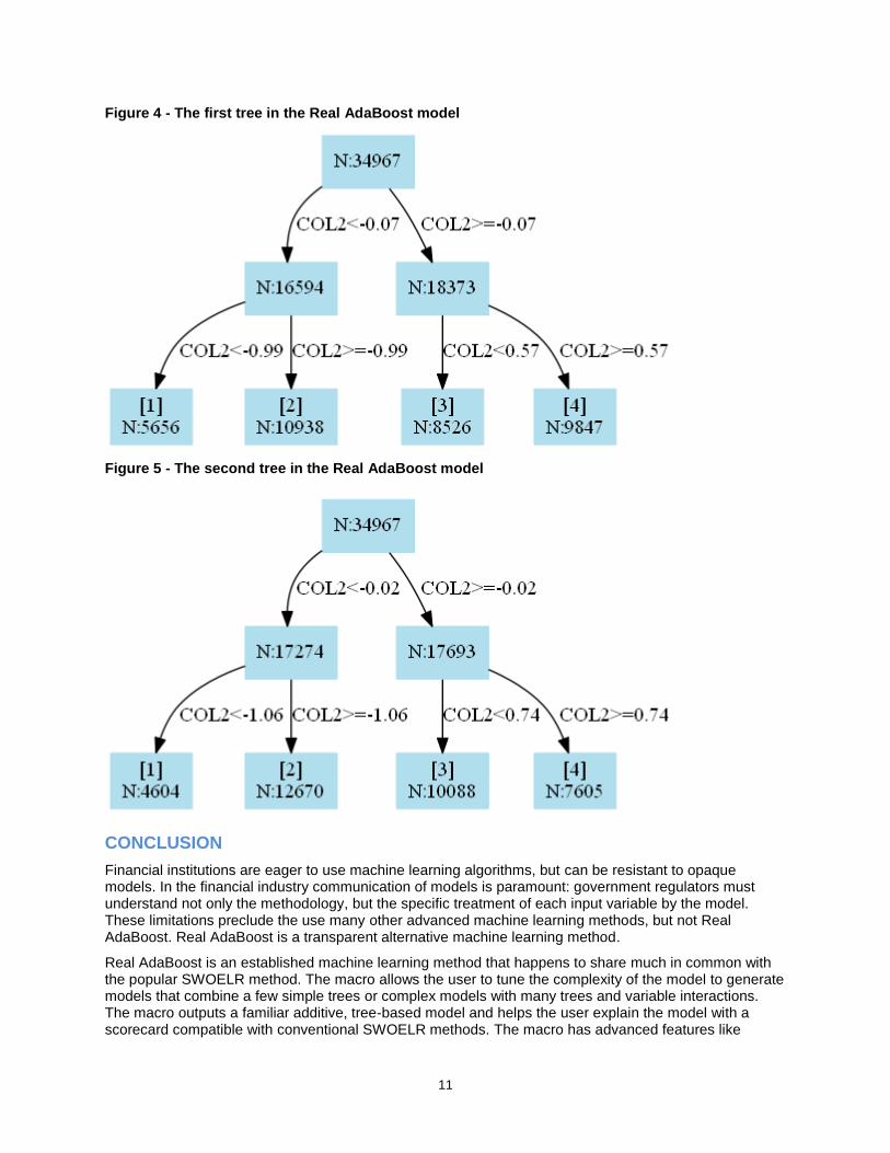
The macro creates *.gv files in the UNIX home directory, which can be processed with the free GraphViz software. GraphViz generates graphical representations of the trees as shown in Figure 4 and Figure 5. The trees can be used to understand the relationships that drive the model predictions. The terminal nodes in the trees correspond to rows of the scorecard.

3 https://en.wikipedia.org/wiki/DOT_(graph_description_language)

4 https://github.com/pedwardsada/real_adaboost

11

Figure 4 - The first tree in the Real AdaBoost model

Figure 5 - The second tree in the Real AdaBoost model

CONCLUSION

Financial institutions are eager to use machine learning algorithms, but can be resistant to opaque models. In the financial industry communication of models is paramount: government regulators must understand not only the methodology, but the specific treatment of each input variable by the model. These limitations preclude the use many other advanced machine learning methods, but not Real AdaBoost. Real AdaBoost is a transparent alternative machine learning method.

Real AdaBoost is an established machine learning method that happens to share much in common with the popular SWOELR method. The macro allows the user to tune the complexity of the model to generate models that combine a few simple trees or complex models with many trees and variable interactions. The macro outputs a familiar additive, tree-based model and helps the user explain the model with a scorecard compatible with conventional SWOELR methods. The macro has advanced features like

12

adaptive binning and automatic variable interaction, and yet requires no fitting of tree coefficients. Real AdaBoost is a powerful method to consider when building your next model.

REFERENCES

Chen, T. and Guestrin, C. 2016. “XGBoost: A Scalable Tree Boosting System”

Freund,Y. and Schapire, R.E. 1997. “A Decision-Theoretic Generalization of On-Line Learning and an Application to Boosting.” Journal of Computer and System Sciences, 55:1 119-139. Available at: http://dx.doi.org/10.1006/jcss.1997.1504.

Friedman, H. Hastie, T., and Tibshirani, R. 2000. “Additive logistic regression: a statistical view of boosting.” The Annals of Statistics, 28(2):337-407. Available at: https://web.stanford.edu/~hastie/Papers/AdditiveLogisticRegression/alr.pdf

Hastie, T., Tibshirani, R., and Friedman, J. 2009. The Elements of Statistical Learning. 10th ed., New York: Springer. Available at: http://statweb.stanford.edu/~tibs/ElemStatLearn/

Maldonado, M., Haller, S., Czika, W., Siddiqi, N.. 2013. “Creating Interval Target Scorecards with Credit Scoring for SAS® Enterprise Miner™”. Proceedings of the SAS Global 2013 Conference. Cary, NC: SAS Institute Inc. Available at https://support.sas.com/resources/papers/proceedings13/094-2013.pdf

Parloff, R. (2016, Oct). “Why Deep Learning Is Suddenly Changing Your Life.” Fortune Magazine. Available at: http://fortune.com/ai-artificial-intelligence-deep-machine-learning/

SAS Institute Inc. 2012. Developing Credit Scorecards Using Credit Scoring for SAS® Enterprise Miner™ 12.1. Cary, NC: SAS Institute Inc.

Schapire, R.E., 2003. The boosting approach to machine learning: An overview. In Nonlinear estimation and classification (pp. 149-171). Springer New York. Available at https://www.cs.princeton.edu/courses/archive/spring07/cos424/papers/boosting-survey.pdf

ACKNOWLEDGMENTS

We wish to thank Gordon Mcgregor for reviewing a draft of this manuscript.

CONTACT INFORMATION

Your comments and questions are valued and encouraged. Contact the author at:

Paul Edwards Scotiabank paul.edwards2@scotiabank.com https://www.linkedin.com/in/paul-edwards-37785391/