Embed Size (px)
Citation preview
1
Metaheuristic Algorithms for Combinatorial Optimization
Massimo [email protected])
010-353 2996
DIST – Università di Genova
Metaheuristic Algorithms - Massimo Paolucci 2
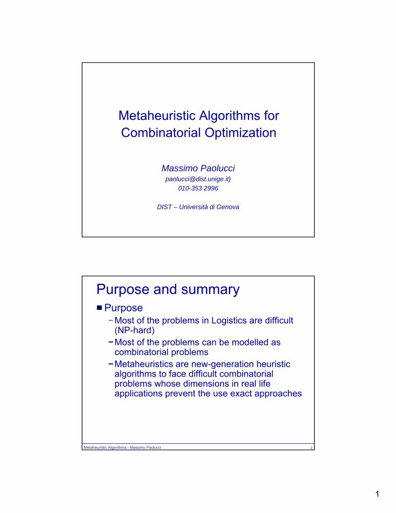
Purpose and summaryPurpose
Most of the problems in Logistics are difficult (NP-hard) Most of the problems can be modelled as combinatorial problemsMetaheuristics are new-generation heuristic algorithms to face difficult combinatorial problems whose dimensions in real life applications prevent the use exact approaches
2
Metaheuristic Algorithms - Massimo Paolucci 3
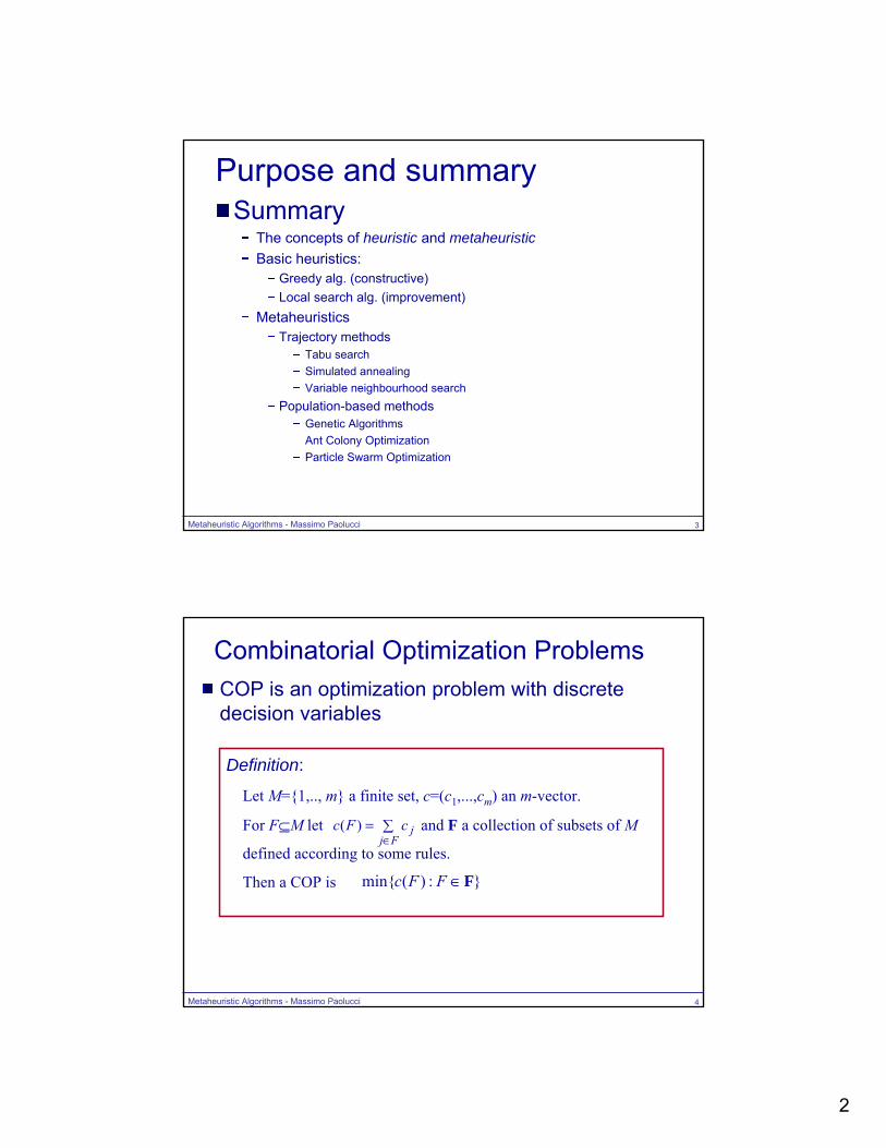
Purpose and summarySummary
The concepts of heuristic and metaheuristicBasic heuristics:
Greedy alg. (constructive)Local search alg. (improvement)
MetaheuristicsTrajectory methods
Tabu searchSimulated annealingVariable neighbourhood search
Population-based methodsGenetic AlgorithmsAnt Colony OptimizationParticle Swarm Optimization
Metaheuristic Algorithms - Massimo Paolucci 4
Combinatorial Optimization ProblemsCOP is an optimization problem with discrete decision variables
Definition:
Let M={1,.., m} a finite set, c=(c1,...,cm) an m-vector.
For F⊆M let and F a collection of subsets of M
defined according to some rules.
Then a COP is
∑=∈Fj
jcFc )(
}:)(min{ F∈FFc

3
Metaheuristic Algorithms - Massimo Paolucci 5
Combinatorial Optimization ProblemsA TSP problem is a COP (1):
Given a graph G=(V, E) let:M={1,.., m} the set of edge indexes E={e1,..., em}, m=|E|c=(c1,...,cm) the edge costsF a collection of subsets F of M such that
F={an edge sequence corresponding to a hamiltonian cycle in G}
Then the TSP is the COP
}:)(min{ F∈FFc
Metaheuristic Algorithms - Massimo Paolucci 6
Combinatorial Optimization ProblemsA TSP problem is a COP (2):
Given a graph G=(V, E) let:N={1,.., n} the set of vertex indexes V={v1,..., vn}, n=|V|D=[dij] an n×n distance matrixF a collection of subsets F of V such that
F={a cyclic permutation π of n items}π (i) the vertex visited after vertex i in π
Then the TSP is the COP }:)(min{ F∈FFc
F∈∀∑===
Fdc(πc(F)n
jjj
1)() π
4
Metaheuristic Algorithms - Massimo Paolucci 7
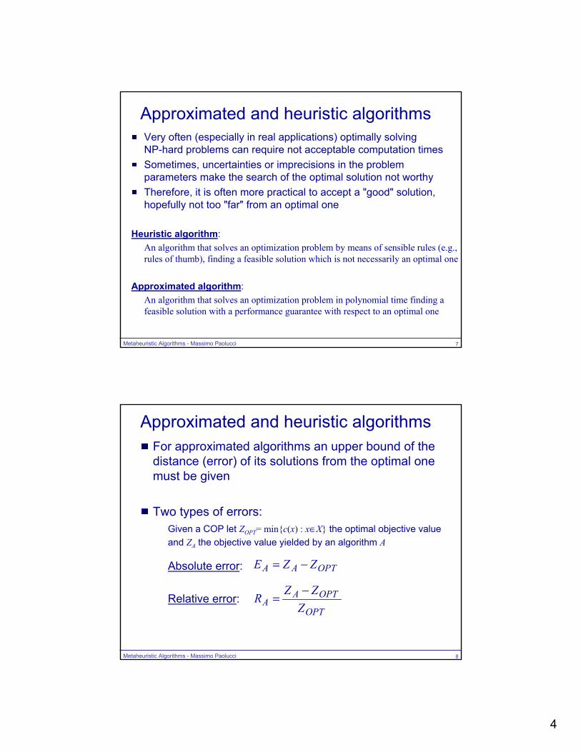
Approximated and heuristic algorithmsVery often (especially in real applications) optimally solving NP-hard problems can require not acceptable computation timesSometimes, uncertainties or imprecisions in the problem parameters make the search of the optimal solution not worthyTherefore, it is often more practical to accept a "good" solution, hopefully not too "far" from an optimal one
Heuristic algorithm:An algorithm that solves an optimization problem by means of sensible rules (e.g., rules of thumb), finding a feasible solution which is not necessarily an optimal one
Approximated algorithm:An algorithm that solves an optimization problem in polynomial time finding a feasible solution with a performance guarantee with respect to an optimal one
Metaheuristic Algorithms - Massimo Paolucci 8
Approximated and heuristic algorithmsFor approximated algorithms an upper bound of the distance (error) of its solutions from the optimal one must be given
Two types of errors:Given a COP let ZOPT= min{c(x) : x∈X} the optimal objective value and ZA the objective value yielded by an algorithm A
Absolute error:
Relative error:
OPTAA ZZE −=
OPT
OPTAA Z
ZZR
−=

5
Metaheuristic Algorithms - Massimo Paolucci 9
Approximated and heuristic algorithmsApproximated algorithms should be preferred when availableNo performance guarantee is defined for heuristic algorithmsApproximated algorithms are not always available or the upper bound for the error they guarantee is not so good (e.g., ≥50%)Design (and prove) an approximated algorithm is often difficultVery often heuristic algorithm are preferred since they are:
simpler to implementgenerally provide good/acceptable performancegenerally faster
Metaheuristic Algorithms - Massimo Paolucci 10
Basic heuristic algorithmsTwo main kinds of classic heuristics:
Constructive heuristicsBuild the solution step by step at each iterationExamples (TSP): Nearest Neighbourhood, Insertion, Christofides alg.
Improvement heuristicsStart from a complete feasible solution and try at each iteration to improve itExamples (TSP): 2-OPT, 3-OPT, Lin-Kernigham
Note that this classification is not comprehensiveE.g., Lagrangean heuristics basically found non-feasible solutions that try to improve towards feasibility
6
Metaheuristic Algorithms - Massimo Paolucci 11
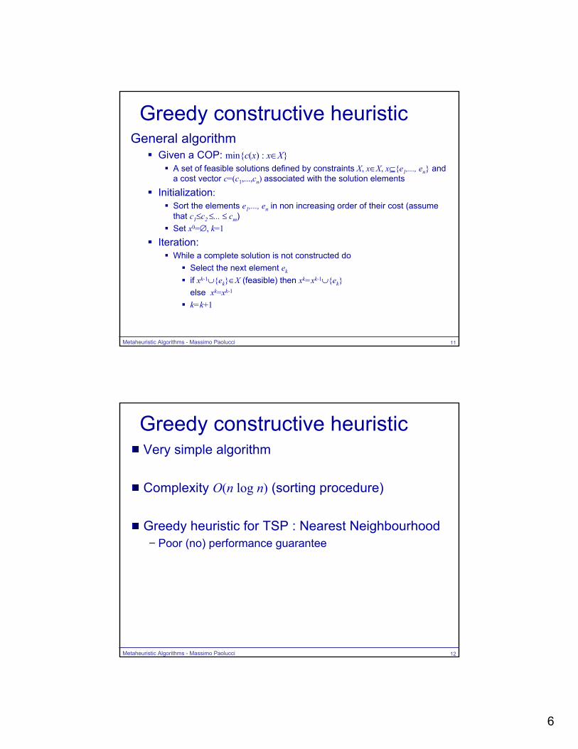
Greedy constructive heuristicGeneral algorithm
Given a COP: min{c(x) : x∈X}A set of feasible solutions defined by constraints X, x∈X, x⊆{e1,..., en} and a cost vector c=(c1,...,cn) associated with the solution elements
Initialization:Sort the elements e1,..., en in non increasing order of their cost (assume that c1≤c2 ≤... ≤ cm)Set x0=∅, k=1
Iteration:While a complete solution is not constructed do
Select the next element ek
if xk-1∪{ek}∈X (feasible) then xk=xk-1∪{ek}else xk=xk-1
k=k+1
Metaheuristic Algorithms - Massimo Paolucci 12
Greedy constructive heuristicVery simple algorithm
Complexity O(n log n) (sorting procedure)
Greedy heuristic for TSP : Nearest NeighbourhoodPoor (no) performance guarantee

7
Metaheuristic Algorithms - Massimo Paolucci 13
Decomposition heuristicGeneral algorithm
Initialization:Decompose the original problem into subproblems with a fixed hierarchy
Iteration:Solve the subproblems starting from the one on the top of the herarchyThe solutions of subproblems are fixed and not revised anymore and may constrain the feasible space of subsequent subproblems
VRP decomposition heuristics:Cluster-First Route-Second
A main clustering problem is solved and then a series of TSPs on the clusters so determined
Route-First Cluster-SecondA main unconstrained TSP problem is solved and then a series of clustering problems conditioned by the service order previously found
Metaheuristic Algorithms - Massimo Paolucci 14
Local Search (LS)LS algorithm is basically an improvement heuristicLS starts from a feasible initial solution and tries to improve it by exploring the solution neighbourhoodLS iterates the exploration step from the new solution until no further improvement is possibleLS is a descent method: it founds a local optimumThe computation time needed by LS (improvement heuristics) is generally much longer than the one of constructive algorithmsLS for COP needs a proper definition of the neighbourhood of solutions
8
Metaheuristic Algorithms - Massimo Paolucci 15
Local Search (LS)Basic LS Algorithm
Initialization:Generate a initial solution xSet the current solution and objective xc=x; Zc= Z(x)
RepeatSet xb=xc; Zb= Zc
For each candidate solution x∈N(xb) If Z(x)<Zc then xc=x; Zc= Z(x)
Until Zc< Zb
N(x) is the neighbourhood of solution xA neighbourhood of x is made of solutions that can be generated by modifying xIf xa∈N(xb) then xb∈N(xa)
Metaheuristic Algorithms - Massimo Paolucci 16
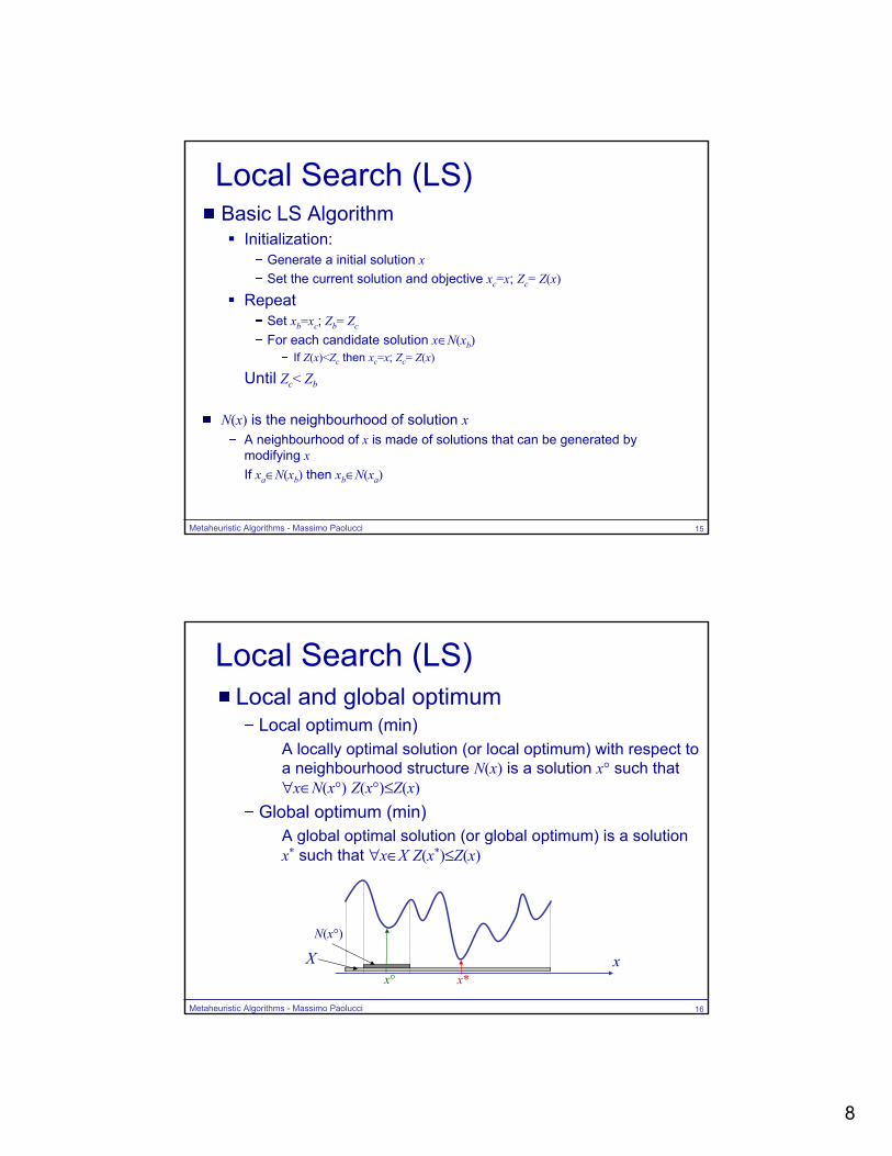
Local Search (LS)Local and global optimum
Local optimum (min)A locally optimal solution (or local optimum) with respect to a neighbourhood structure N(x) is a solution x° such that ∀x∈N(x°) Z(x°)≤Z(x)
Global optimum (min)A global optimal solution (or global optimum) is a solution x* such that ∀x∈X Z(x*)≤Z(x)
xx*x°
XN(x°)
9
Metaheuristic Algorithms - Massimo Paolucci 17
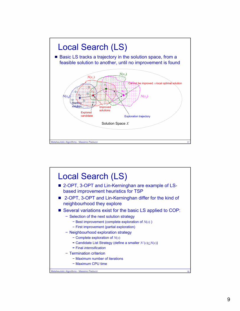
Local Search (LS)Basic LS tracks a trajectory in the solution space, from a feasible solution to another, until no improvement is found
Solution Space X
Starting solution
N(x0)x0
Explored candidate
Improved solutions
x1
x2
x3
Cannot be improved ⇒local optimal solution
Exploration trajectory
N(x1)N(x2)
N(x3)
Metaheuristic Algorithms - Massimo Paolucci 18
Local Search (LS)2-OPT, 3-OPT and Lin-Kerninghan are example of LS-based improvement heuristics for TSP2-OPT, 3-OPT and Lin-Kerninghan differ for the kind of
neighbourhood they exploreSeveral variations exist for the basic LS applied to COP:
Selection of the next solution strategyBest improvement (complete exploration of N(x) )First improvement (partial exploration)
Neighbourhood exploration strategyComplete exploration of N(x)Candidate List Strategy (define a smaller N’(x)⊆N(x))Final intensification
Termination criterionMaximum number of iterationsMaximum CPU time
10
Metaheuristic Algorithms - Massimo Paolucci 19
Local Search (LS)The starting solution x0 does not need to be an high quality one
It is convenient to iterate the whole LS starting from differentinitial solutions (Multi-Start LS - MSLS):
In MSLS the starting solutions are usually randomly generates
Often LS is applied as final intensification step of constructive heuristics:
purpose: to discover if the constructed solution can be trivially improved
Metaheuristic Algorithms - Massimo Paolucci 20
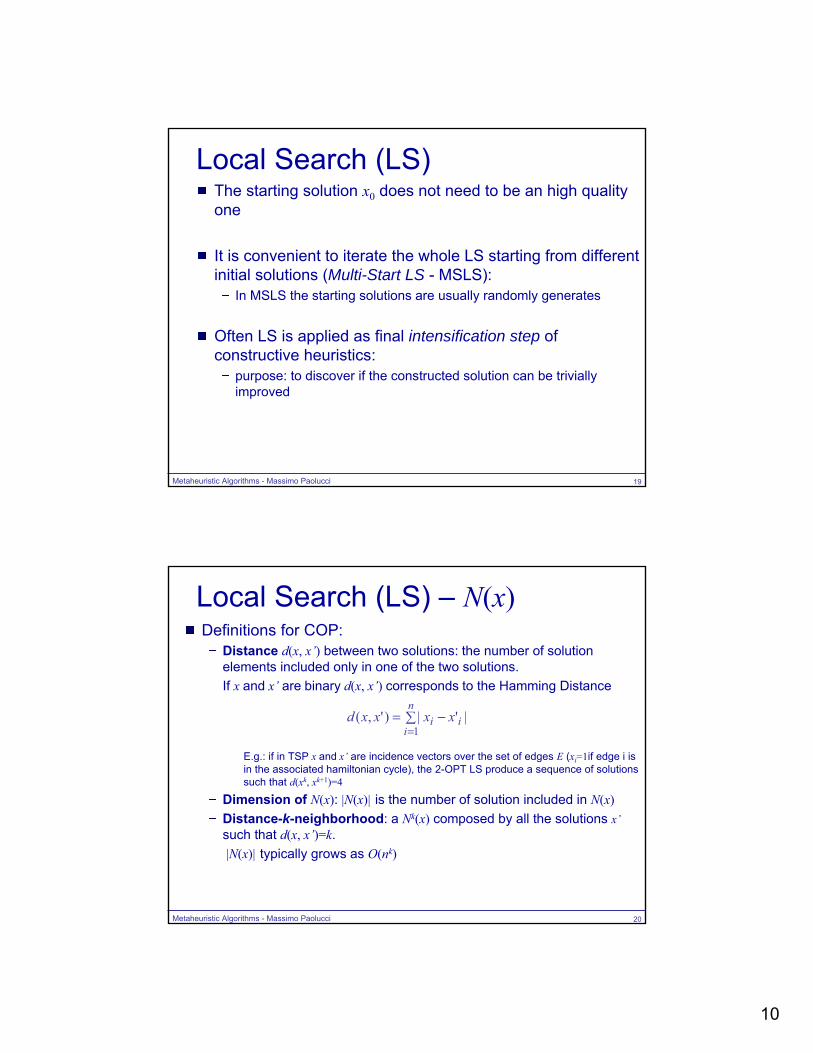
Local Search (LS) – N(x)Definitions for COP:
Distance d(x, x’) between two solutions: the number of solution elements included only in one of the two solutions. If x and x’ are binary d(x, x’) corresponds to the Hamming Distance
E.g.: if in TSP x and x’ are incidence vectors over the set of edges E (xi=1if edge i is in the associated hamiltonian cycle), the 2-OPT LS produce a sequence of solutions such that d(xk, xk+1)=4
Dimension of N(x): |N(x)| is the number of solution included in N(x)Distance-k-neighborhood: a Nk(x) composed by all the solutions x’such that d(x, x’)=k. |N(x)| typically grows as O(nk)
∑ −==
n
iii xxxxd
1|'|)',(
11
Metaheuristic Algorithms - Massimo Paolucci 21
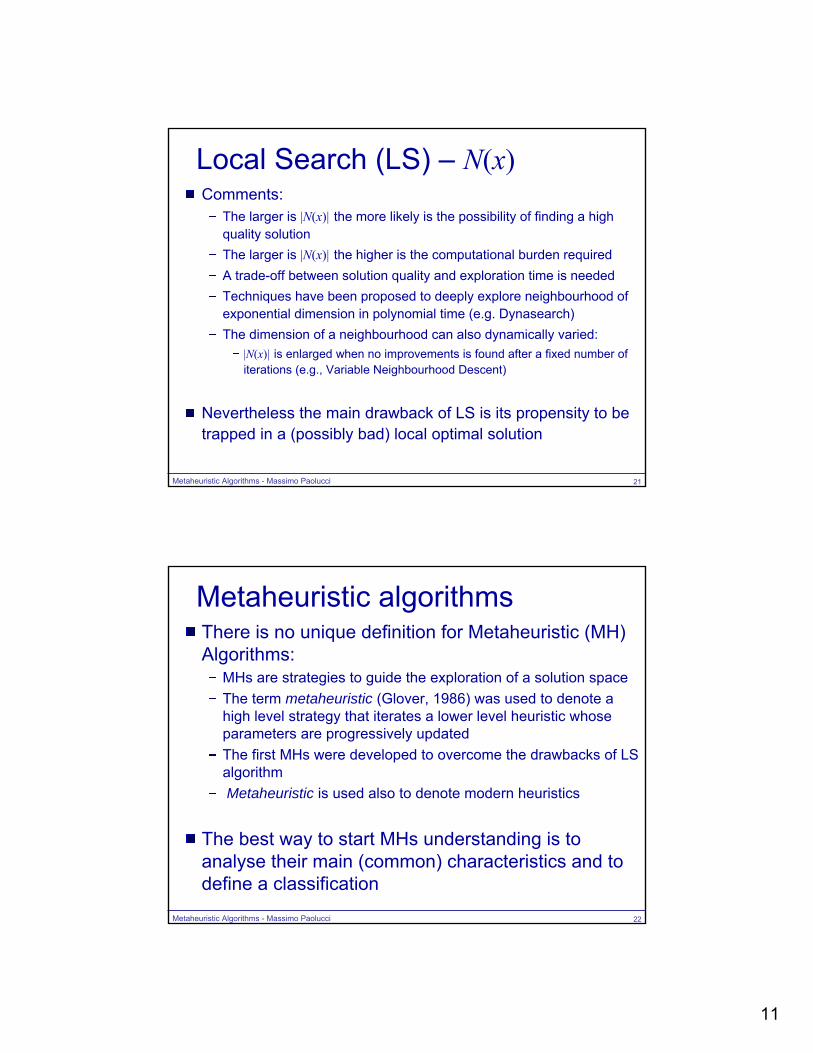
Local Search (LS) – N(x)Comments:
The larger is |N(x)| the more likely is the possibility of finding a high quality solutionThe larger is |N(x)| the higher is the computational burden requiredA trade-off between solution quality and exploration time is neededTechniques have been proposed to deeply explore neighbourhood ofexponential dimension in polynomial time (e.g. Dynasearch)The dimension of a neighbourhood can also dynamically varied:
|N(x)| is enlarged when no improvements is found after a fixed number of iterations (e.g., Variable Neighbourhood Descent)
Nevertheless the main drawback of LS is its propensity to be trapped in a (possibly bad) local optimal solution
Metaheuristic Algorithms - Massimo Paolucci 22
Metaheuristic algorithmsThere is no unique definition for Metaheuristic (MH) Algorithms:
MHs are strategies to guide the exploration of a solution spaceThe term metaheuristic (Glover, 1986) was used to denote a high level strategy that iterates a lower level heuristic whose parameters are progressively updatedThe first MHs were developed to overcome the drawbacks of LS algorithmMetaheuristic is used also to denote modern heuristics
The best way to start MHs understanding is to analyse their main (common) characteristics and to define a classification
12
Metaheuristic Algorithms - Massimo Paolucci 23
Metaheuristic algorithmsTwo possible definitions:
“A metaheuristic is formally defined as an iterative generation process which guides a subordinate heuristic by combining intelligently different concepts for exploring and exploiting the search space, learning strategies are used to structure information in order to find efficiently near-optimal solutions.” (Osman and Laporte 1996)
“A metaheuristic is an iterative master process that guides and modifies the operations of subordinate heuristics to efficiently produce high-quality solutions. It may manipulate a complete (or incomplete) single solution or a collection of solutions at each iteration. The subordinate heuristics may be high (or low) level procedures, or a simple local search, or just a construction method.” (Voß et al. 1999)
Metaheuristic Algorithms - Massimo Paolucci 24
Metaheuristic algorithmsCharacteristics (Blum and Roli, 2003):
MHs are strategies that “guide” the search process.The goal is to efficiently explore the search space in order to find (near) optimal solutions.Techniques which constitute MH algorithms range from simple local search procedures to complex learning processes.MH algorithms are approximate and usually non-deterministic.MH may incorporate mechanisms to avoid getting trapped in confined areas of the search space.The basic concepts of MHs permit an abstract level description.MHs are not problem-specific.MHs may make use of domain-specific knowledge in the form of heuristics that are controlled by the upper level strategy.Todays more advanced MHs use search experience (embodied in some form of memory) to guide the search.

13
Metaheuristic Algorithms - Massimo Paolucci 25
Metaheuristic algorithmsMH “philosophies”:Intelligent extensions of LS algorithms (Trajectory methods):
The goal is to escape from local minima in order to proceed in the exploration of the search space and to move on to find other hopefully better local minima. They use one or more neighbourhood structure(s) Examples: Tabu Search, Iterated Local Search, Variable Neighbourhood Search, GRASP and Simulated Annealing
Use of learning components (Learning Population-based methods):They implicitly or explicitly try to learn correlations between decision variables to identify high quality areas in the search space. They perform a biased sampling of the search spaceExamples: Ant Colony Optimization, Particle Swarm Optimization and Evolutionary Computation.
Metaheuristic Algorithms - Massimo Paolucci 26
Metaheuristic algorithmsPossible MH classifications:
Nature-inspired vs non-nature inspired
Population-based vs single point search
Dynamic vs static objective function
One vs various neighbourhood structures
Memory usage vs memory-less methods
14
Metaheuristic Algorithms - Massimo Paolucci 27
Metaheuristic algorithmsMHs outline:
Trajectory methods:Tabu SearchSimulated AnnealingVariable Neighbourhood Search
Population-based methods:Evolutionary Computation (Genetic Algorithms)Ant Colony OptimizationParticle Swarm Optimization
Metaheuristic Algorithms - Massimo Paolucci 28
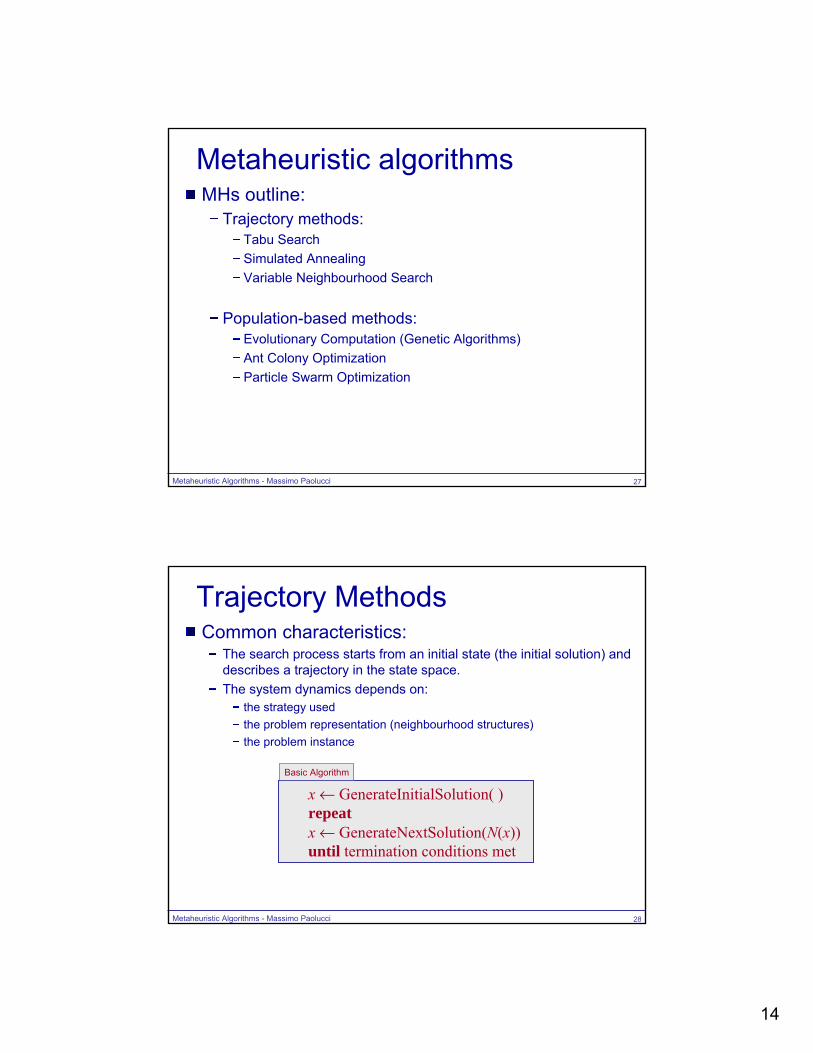
Trajectory MethodsCommon characteristics:
The search process starts from an initial state (the initial solution) and describes a trajectory in the state space. The system dynamics depends on:
the strategy usedthe problem representation (neighbourhood structures) the problem instance
x ← GenerateInitialSolution( )repeatx ← GenerateNextSolution(N(x))until termination conditions met
Basic Algorithm

15
Metaheuristic Algorithms - Massimo Paolucci 29
Tabu Search (TS)A deterministic method first introduced by Glover (1986)TS explicitly uses the history of the search, both to escape from local minima and to implement an explorative strategyTS is an extended LS since it can continue the exploration after a local optimal solution is foundThe Tabu List (TL) is a short-term memory to escape from local optima
x ← GenerateInitialSolution( )TabuList ← ∅while termination conditions not metx ← ChooseBestOf(N(x)\TabuList )Update(TabuList)endwhile
Basic TS
TL keeps memory of the recent search history
The next solution may not improve the current one
Metaheuristic Algorithms - Massimo Paolucci 30
Tabu Search (TS)The TL restricts the neighbourhood of the current solution
The Tabu List: a FIFO list list dimension n ⇒ Tabu Tenurestore information about the latest solutions of the exploration trajectory used to forbid the selection of solutions recently visited (cycling)
TabuListxNxAllowed \)()( =
xkxk+1xk-1xk+n-2xk+n-1xk+n ...
n
previous current solution
next current solution

16
Metaheuristic Algorithms - Massimo Paolucci 31
Tabu Search (TS)TS vs LS
Solution Space X
Starting solution
N(x0)x0
x1
x2x3
Local optimal solution
N(x1) N(x2)
N(x3)
Solution Space X
Starting solution
N(x0)x0
x1
x2
x3
Local optimal solution
N(x1)N(x2)
N(x3)
Local Search
Tabu SearchForbidden (in the TL)
Best in N(x3)\TL
N(x4)x4
Next improved solution
x5
x0 x1 x2 x4x3 x5
Z(x)
Metaheuristic Algorithms - Massimo Paolucci 32
Tabu Search (TS)The TL restricts the neighbourhood of the current solutionTL prevents from returning to recently visited solutions (cycling)TL forces the search to accept even uphill movesThe tabu tenure controls the memory of the search process:
Small ⇒ the search concentrates on small areas of the search spaceLarge ⇒ the search process is forced to explore larger regions
The tabu tenure can be fixed or varied during the search
17
Metaheuristic Algorithms - Massimo Paolucci 33
Tabu Search (TS)Storing complete solutions in the TL is highly inefficient TL usually stores solution attributes :
solution componentsmovesdifferences between two solutions
A single or more attributes ⇒ a single or more TLsThe set of TLs define the tabu conditions filtering N(x)Storing attributes ⇒ loss of information:
the tabu status assigned to more than one solution ⇒ unvisited good solutions may be excluded
Aspiration criteria: allow promising solutions that are forbidden
Best Objective criterion
Metaheuristic Algorithms - Massimo Paolucci 34
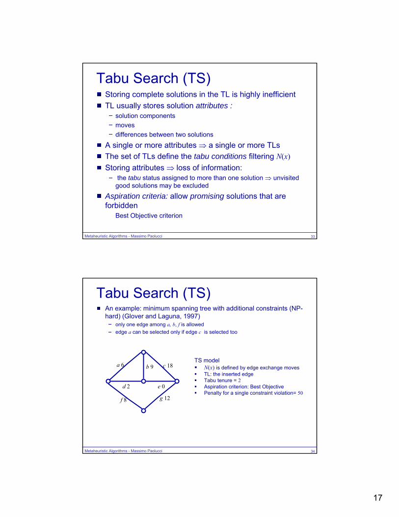
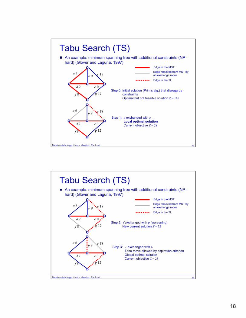
Tabu Search (TS)An example: minimum spanning tree with additional constraints (NP-hard) (Glover and Laguna, 1997)
only one edge among a, b, f is allowededge a can be selected only if edge c is selected too
a 6 c 18
f 8 g 12
d 2 e 0
b 9TS model
N(x) is defined by edge exchange moves TL: the inserted edgeTabu tenure = 2Aspiration criterion: Best ObjectivePenalty for a single constraint violation= 50
18
Metaheuristic Algorithms - Massimo Paolucci 35
Tabu Search (TS)An example: minimum spanning tree with additional constraints (NP-hard) (Glover and Laguna, 1997)
a 6 c 18
f 8 g 12
d 2 e 0
b 9
Step 0: Initial solution (Prim’s alg.) that disregards constraintsOptimal but not feasible solution Z = 116
Step 1: a exchanged with cLocal optimal solutionCurrent objective Z = 28
Edge in the MSTEdge removed from MST by an exchenge move
Edge in the TL
a 6 c 18
f 8 g 12
d 2 e 0
b 9
Metaheuristic Algorithms - Massimo Paolucci 36
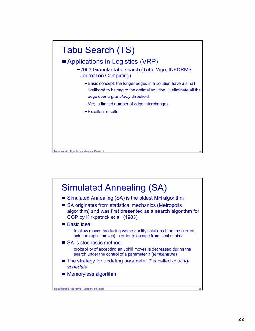
Tabu Search (TS)An example: minimum spanning tree with additional constraints (NP-hard) (Glover and Laguna, 1997)
a 6 c 18
f 8 g 12
d 2 e 0
b 9
Step 2: f exchanged with g (worsening)New current solution Z = 32
Step 3: c exchanged with bTabu move allowed by aspiration criterionGlobal optimal solutionCurrent objective Z = 23
Edge in the MSTEdge removed from MST by an exchenge move
Edge in the TL
a 6 c 18
f 8 g 12
d 2 e 0
b 9

19
Metaheuristic Algorithms - Massimo Paolucci 37
Tabu Search (TS)Candidate List Strategies (CLS):
Used to heuristically restrict the N(x) dimension to the subset of most promising solutions (e.g., execute the moves that should produce the greater improvements)
Long-Term Memory (LTM) can be used for :Storing elite complete solutions: quality solutions whose improvement require a great number of iterationsStoring solution attributes frequent appeared during the search
TS may include two mechanisms based on LTM:Intensification: a thorough LS is finally executed starting from elite solutions (especially if CLS are used)Diversification: it forces the search to abandon the already visited regions of the solution space after a fixed number of iteration without any improvements (non-improving iterations)
Metaheuristic Algorithms - Massimo Paolucci 38
Tabu Search (TS)x ← GenerateInitialSolution( ) InitializeTabuLists(TL1,..., TLr )k ←0kNI ←0while termination conditions not met
AllowedSet(x, k)←{x’∈N(x): not ViolateTabuCond(x’) or SatisfyAspirCrit(x’)}xc ← ChooseBestOf(AllowedSet(x, k))if Improve(xc, x) then kNI ←0else kNI ← kNI +1x ←xc
CheckAndUpdateEliteSolutions( )UpdateTabuListsAndAspirationConditions( )k ←k+1if kNI > MaxNonImprovingIteration then Divesification( )
endwhileIntesificationFromEliteSolutions( )
General TS

20
Metaheuristic Algorithms - Massimo Paolucci 39
Tabu Search (TS)Applications in Logistics (VRP)
1989 First TS implementation (Willard, M.Sc. thesis, Imperial College)
a solution transformed in a giant tour by replicating the depot
N(x): feasible solutions reached by a 2-opt or 3-opt moves
next solution: best non tabu move
not competitive with known approximation approach
1991 Second TS implementation (Pureza and França)N(x): feasible solutions obtained by moving a vertex to a different route or swapping vertices
not particularly good results
Metaheuristic Algorithms - Massimo Paolucci 40
Tabu Search (TS)Applications in Logistics (VRP)
1991 First version of Taburoute (Gendreau, Hertz, Laporte, Tristan I Conference)
N(x): feasible solutions reached by moving a vertex to a different route containing one of its p nearest neighbours
after each insertion a local re-optimization is performed (GENI+US)
may accept not feasible solutions (max capacity or duration) butpenalize violations with adjustable weights ⇒ favour excaping from local optima
random tabu tags instead of TL (a move executed at t is tabu for t+δ with δ ~U[5, 10])
diversification (frequently moved vertices are penalized)
false starts

21
Metaheuristic Algorithms - Massimo Paolucci 41
Tabu Search (TS)Applications in Logistics (VRP)
1993 Taillard (Networks)Similar to Taburoute (random tabu tags, diversification)
N(x): λ-interchanges (combination of λ-opt, vertex reassignments to different routes, vertex interchanges between two routes)
Standard insertion (not GENI) maintaining feasibility
Initial problem decomposition (in planar problem: sector centred in the depot and concentric areas) and move of vertices between adjacent sectors
Metaheuristic Algorithms - Massimo Paolucci 42
Tabu Search (TS)Applications in Logistics (VRP)
2001 Unified tabu search algorithm (Cordeau, Laporte, Mercier, Journal of the Operational Research Society)
Several of the features of Taburoute (GENI insertions, intermediate infeasible solutions and long-term frequency based penalties)single initial solution, fixed tabu durations, no intensificationtabu on an attribute set B(x) = {(i, k) : vi is visited by vehicle k in solution x}N(x): remove (i, k) from B(x) replacing it with (i, k’) with k≠ k’Attribute (i, k) is tabu for a number of iterationsaspiration criterionVery few parameters and flexible (applied with success to many VRP variants)
22
Metaheuristic Algorithms - Massimo Paolucci 43
Tabu Search (TS)Applications in Logistics (VRP)
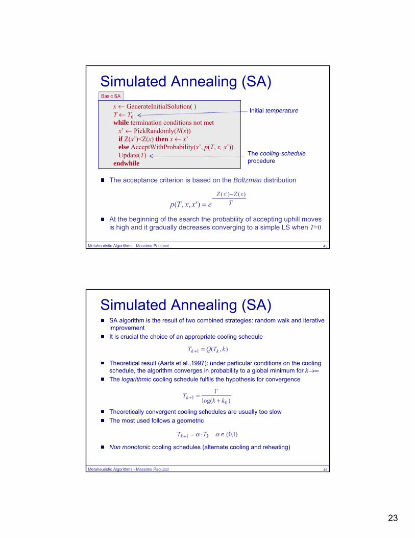
2003 Granular tabu search (Toth, Vigo, INFORMS Journal on Computing)
Basic concept: the longer edges in a solution have a small likelihood to belong to the optimal solution ⇒ eliminate all the edge over a granularity threshold
N(x): a limited number of edge interchanges
Excellent results
Metaheuristic Algorithms - Massimo Paolucci 44
Simulated Annealing (SA)Simulated Annealing (SA) is the oldest MH algorithmSA originates from statistical mechanics (Metropolis algorithm) and was first presented as a search algorithm for COP by Kirkpatrick et al. (1983) Basic idea:
to allow moves producing worse quality solutions than the current solution (uphill moves) in order to escape from local minima
SA is stochastic method:probability of accepting an uphill moves is decreased during thesearch under the control of a parameter T (temperature)
The strategy for updating parameter T is called cooling-scheduleMemoryless algorithm
23
Metaheuristic Algorithms - Massimo Paolucci 45
Simulated Annealing (SA)
The acceptance criterion is based on the Boltzman distribution
At the beginning of the search the probability of accepting uphill moves is high and it gradually decreases converging to a simple LS when T=0
x ← GenerateInitialSolution( )T ← T0while termination conditions not met
x’ ← PickRandomly(N(x))if Z(x’)<Z(x) then x ← x’else AcceptWithProbability(x’, p(T, x, x’))Update(T)
endwhile
Basic SA
The cooling-scheduleprocedure
Initial temperature
TxZxZ
exxTp)()'(
)',,(−−
=
Metaheuristic Algorithms - Massimo Paolucci 46
Simulated Annealing (SA)SA algorithm is the result of two combined strategies: random walk and iterative improvementIt is crucial the choice of an appropriate cooling schedule
Theoretical result (Aarts et al.,1997): under particular conditions on the cooling schedule, the algorithm converges in probability to a global minimum for k→∞The logarithmic cooling schedule fulfils the hypothesis for convergence
Theoretically convergent cooling schedules are usually too slow The most used follows a geometric
Non monotonic cooling schedules (alternate cooling and reheating)
),(1 kTQT kk =+
)log( 01 kk
Tk +Γ=+
)1,0(1 ∈⋅=+ αα kk TT

24
Metaheuristic Algorithms - Massimo Paolucci 47
Simulated Annealing (SA)Applications in Logistics
1993 Simulated Annealing and local search (Osman,Annals of Operations Research)
N(x): λ-interchange generation mechanism (two route are selected with two subsets of vertices with cardinality less than λ, and the vertices in the two sets are swapped as long this is feasible) (λ=1 or 2)Two phases:
Descent alg. (determine a good starting solution from Clark and Wright heuristic and a LS)SA with a cooling schedule that decrease and increase the temperature depending on the quality of the solution found at each iteration
2004 Deterministic annealing (Li, Golden, Wasil, Computers & Operations Research)
Similar to SA but with a deterministic solution acceptance rule
Metaheuristic Algorithms - Massimo Paolucci 48
Variable neighbourhood search (VNS)VNS proposed by Hansen and Mladenovć (1999, 2001)Idea: improve the LS process with a strategy that dynamically change the neighborhood structure A very general algorithm with many degrees of freedomInitialization: define a set of neighborhood structures arbitrarily chosenOften a sequence |N1|<|N2|<...<|Nkmax| with increasing cardinality is usedThe main cycle is composed of three phases:
shakinglocal searchmove

25
Metaheuristic Algorithms - Massimo Paolucci 49
Variable neighbourhood search (VNS)
Note that LS is not restricted to explore the set of Nk(x)
Select a set of neighborhood structures Nk , k=1,... , kmaxx ← GenerateInitialSolution( )while termination conditions not met
k ← 1while k<kmax
x’ ← PickRandomly(Nk(x))x” ← LocalSearch(x’)if Z(x”)<Z(x) then
x ← x”k ← 1
else k ← k +1endif
endwhileendwhile
Basic VNS
Shaking Phase
Inner loop
LS Phase
Move Phase
Metaheuristic Algorithms - Massimo Paolucci 50
Variable neighbourhood search (VNS)Comments:
The shaking phase perturbs x to find a good starting point x’ for LSx’ should belong to the basin of attraction of a local minimum different from the current one, but should not “too far” from it (to avoid the algorithm degenerate into a simple random multi-start)x’ in Nk(x) is likely to maintains some good features of the current x
Changing neighbourhood (no improvements) ⇒ diversification
Core idea: A solution locally optimal with respect to a neighbourhood is probably not locally optimal with respect to another neighbourhoodThe neighbourhood structure determines the topological properties of the search landscapeThe properties of a landscape are in general different from those of other landscapes

26
Metaheuristic Algorithms - Massimo Paolucci 51
Variable neighbourhood search (VNS)
x
x*x°
Nk+1(x°)
x
x*x°
Nk(xi)
xi x’
x
x*x’Nk+1(x’)
Shaking
LS
LS
Changing neighbourhood (k+1) ⇒ changing landscape
Metaheuristic Algorithms - Massimo Paolucci 52
Variable neighbourhood search (VNS)Variant: Variable Neighbourhood Descent (VND)
Select a set of neighborhood structures Nk , k=1,... , kmaxx ← GenerateInitialSolution( )
while termination conditions not metk ← 1while k<kmax
x’ ← ChooseBestOf(Nk(x))if Z(x’)<Z(x) then x ← x’else k ← k +1endif
endwhileendwhile
VND
LS Phase in Nk(x)
k not reset to 1

27
Metaheuristic Algorithms - Massimo Paolucci 53
Variable neighbourhood search (VNS)Applications in Logistics
Pickup-and-Delivery TSP with LIFO loading (Cassani, L., G. Righini. 2004) (Carrabs, Cordeau, Laporte 2005)
definition of new operators to generate neighbourhoodA Reactive Variable Neighborhood Search for the Vehicle-Routing Problem with Time Windows (Bräysy, 2003)
VND based methodBoth inter-route and intra-route exchange operators
Multi-Depot Vehicle Routing Problems with Time Windows (Polaceck, Hart, Doener, 2005):
neighbourhoods generated by CROSS-exchange (Taillard et al.,1997) and inverted-CROSS exchange operatorsparameters are the length of the exchanged segment and the number of depots involvedexperiments showed good performance
Metaheuristic Algorithms - Massimo Paolucci 54
Population-based methodsCommon characteristics:
At every iteration search process considers a set (a population) of solutions instead of a single oneThe performance of the algorithms depends on the way the solution population is manipulatedTake inspiration from natural phenomenaThree approaches:
Evolutionary Computation (Genetic Algorithms)Ant Colony OptimizationParticle Swarm Optimization
28
Metaheuristic Algorithms - Massimo Paolucci 55
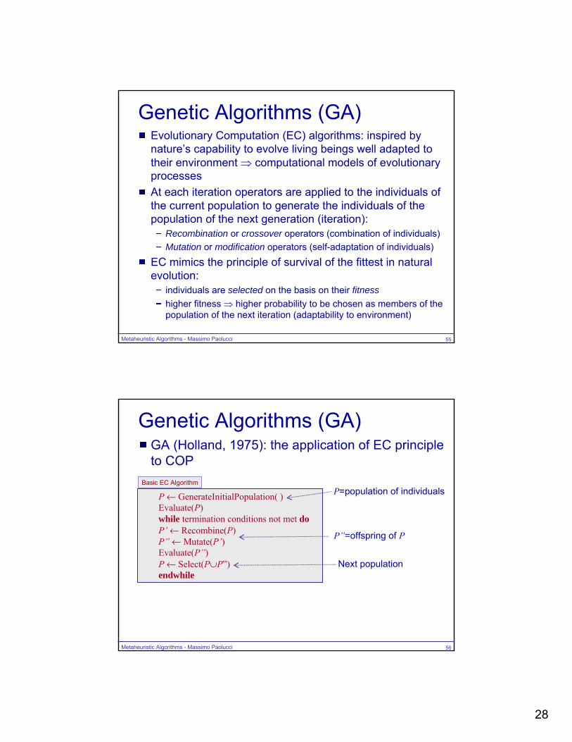
Genetic Algorithms (GA)Evolutionary Computation (EC) algorithms: inspired by nature’s capability to evolve living beings well adapted to their environment ⇒ computational models of evolutionary processesAt each iteration operators are applied to the individuals of the current population to generate the individuals of the population of the next generation (iteration):
Recombination or crossover operators (combination of individuals)Mutation or modification operators (self-adaptation of individuals)
EC mimics the principle of survival of the fittest in natural evolution:
individuals are selected on the basis on their fitnesshigher fitness ⇒ higher probability to be chosen as members of the population of the next iteration (adaptability to environment)
Metaheuristic Algorithms - Massimo Paolucci 56
Genetic Algorithms (GA)GA (Holland, 1975): the application of EC principle to COP
P ← GenerateInitialPopulation( )Evaluate(P)while termination conditions not met doP’ ← Recombine(P)P” ← Mutate(P’)Evaluate(P”)P ← Select(P∪P”)endwhile
Basic EC AlgorithmP=population of individuals
P”=offspring of P
Next population

29
Metaheuristic Algorithms - Massimo Paolucci 57
Genetic Algorithms (GA)Individuals:
solutions, partial solutions, sets of solutions, any object which can be transformed into one or more solutions in a structured wayIn COP bit-strings or permutations of integers are often used
GA:Individuals ⇒ genotypessolutions encoded by individuals ⇒ phenotypes
Crucial aspect: the choice of an appropriate representation
Metaheuristic Algorithms - Massimo Paolucci 58
Genetic Algorithms (GA)An example (bit string)
)1,0,0,1,1,0(=x
100110
Chromosome
Gene
Solution100110
001011
100111
Single point crossover (random)
Parents
Offspring
Ax
Bx
001010
crossover
mutation
100111
Mutation (random)
100101

30
Metaheuristic Algorithms - Massimo Paolucci 59
Genetic Algorithms (GA)An example: a sequencing problem – TSP
Vertex sequences instead of a bit strings
152340543210Position
Vertex
01
5 4 3
2
Metaheuristic Algorithms - Massimo Paolucci 60
Genetic Algorithms (GA)An example: a sequencing problem – TSP
Straightforward one-point crossover
152340Parent 1
Cut point
543210Parent 2
Offspring 1
Offspring 2
543340
152210Not feasible

31
Metaheuristic Algorithms - Massimo Paolucci 61
Genetic Algorithms (GA)An example: a sequencing problem – TSP
Specialized crossover operator: an example Order Crossover (OX) (Oliver, Smith, Holland, 1987)
the offspring inherits the relative order of the parents
152340Parent 1
Two cut points
543210Parent 2
Offspring 1 452310
Metaheuristic Algorithms - Massimo Paolucci 62
Genetic Algorithms (GA)An example: a sequencing problem – TSP
Mutation operator: Simple insert (remove and reinsert – RAR) or swap moves
451320Mutated Offspring 1
mutation
Offspring 1 452310

32
Metaheuristic Algorithms - Massimo Paolucci 63
Genetic Algorithms (GA)Evolution Process
At each iteration which individuals will enter the population of the next iteration is decided by a selection scheme:
generational replacement: the individuals for the next population are selected exclusively from the offspringsteady state evolution process: it is possible to transfer individuals of the current population into the next population
Fixed population size vs variable population size In case of shrinking population size a situation where only one individual is left in the population (or no crossover partners can be found for any member of the population) might be one of the stopping conditions of the algorithm
Metaheuristic Algorithms - Massimo Paolucci 64
Genetic Algorithms (GA)Neighbourhood Structure
∀i∈I NEC(i)⊆I assigns to every individual a set of individuals which are permitted to act as recombination partners for i to create offspringStructured vs Unstructured populations: in unstructured populations individuals can be recombined with any other individual (e.g., in simple GA)
Information Sources (to create offspring)The most commonly used: a couple of parents (two-parent crossover)Generally recombination operators may operate on more than two individuals to create a new individual (multi-parent crossover)

33
Metaheuristic Algorithms - Massimo Paolucci 65
Genetic Algorithms (GA)Infeasibility
Recombining individuals, the offspring might be potentially infeasible. Three basic strategies:
reject (simplest)penalizing infeasible individuals in the quality functionrepair
Intensification StrategyApplication of LS to improve the fitness of individuals. Approaches with LS applied to every individual of a population are often called Memetic AlgorithmsLinkage learning or building block learning: a strategy that uses recombination operators to explicitly try to combine “good” parts of individuals (rather than, e.g., a simple one-point crossover for bit-strings)
Metaheuristic Algorithms - Massimo Paolucci 66
Genetic Algorithms (GA)Diversification Strategy
Purpose: avoid the premature convergence into sub-optimal solutions
The simplest diversification mechanism: use a mutation operator ⇒ a small random perturbation of an individual that introduces a kind of noiseTechniques to maintain the population diversity:
preselection: offspring replace the parent only if the offspring's fitness exceeds that of the inferior parentcrowding: offspring are compared with a few (typically 2 or 3) randomly-chosen individuals from the population. The offspring replaces the most similar one found

34
Metaheuristic Algorithms - Massimo Paolucci 67
Genetic Algorithms (GA)Applications in Logistics
Many TSP applications but rather scarce for VRP Some effective implementations for VRPTW (Potwin, Bengio, 1996)Comparison of GA+LS with TS and SA (Van Breedam, 1996):
similar performance but greater computation timeimportant role of LS (memetic)
CVRP (time constrained) (Schmitt, 1994, 1995)GA for the route phase of a route-first cluster-second approach (clustering is based on a sweep procedure)OX crossover with random 2-opt LSnot clear effectiveness
VRPBaker, Ayechew 2003: GA model a GAP to assign customers to vehicles + TSPDVRP: Prins, 2004, Mester and Bräysy, 2004 (AGES): chromosome=giant tour + optimal splitting proc.Lacomme, Prins, Sevaux, 2006: bi-objective CARP
Metaheuristic Algorithms - Massimo Paolucci 68
Ant Colony Optimization (ACO)ACO was introduced by Dorigo in his PhD thesis (1992)Natural inspiration
The foraging behaviour of real ants that enables ants to find shortest paths between food sources and their nest
While walking from food sources to the nest and vice versa, antsdeposit on the ground an essence, the pheromoneWhen they decide about a direction to go, they choose with higher probability paths that are marked by stronger pheromone concentrations. This basic behaviour is the basis for a cooperative interaction which leads to the emergence of shortest paths

35
Metaheuristic Algorithms - Massimo Paolucci 69
Ant Colony Optimization (ACO)The behaviour of real ants
Metaheuristic Algorithms - Massimo Paolucci 70
Ant Colony Optimization (ACO)Example: a group of 30 ants leaves every minute the nest searching food
A
B
C
30 ants
H
D
E
15 ants 20 ants
30 ants
15 ants 15 ants
t=0
dABHDE=1dABCDE=0.5
A
B
C
30 ants
H
D
E
15 ants
t=1
τ=30τ=15
10 ants
τ=0τ=0A
B
CH
D
E
15 ants
15 ants
15 ants
t=0.5
τ=15τ=0
36
Metaheuristic Algorithms - Massimo Paolucci 71
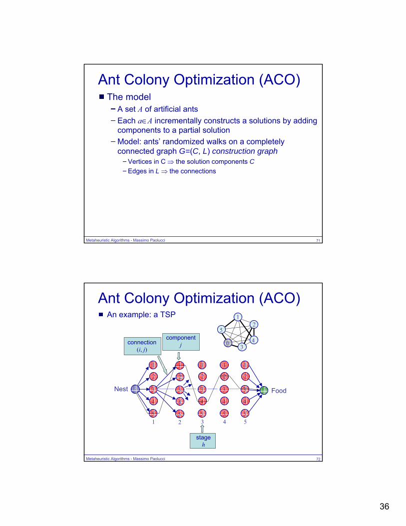
Ant Colony Optimization (ACO)The model
A set A of artificial antsEach a∈A incrementally constructs a solutions by adding components to a partial solution Model: ants’ randomized walks on a completely connected graph G=(C, L) construction graph
Vertices in C ⇒ the solution components C Edges in L ⇒ the connections
Metaheuristic Algorithms - Massimo Paolucci 72
An example: a TSP
Ant Colony Optimization (ACO)
1
Nest Food
1
2
3
4
52
1
2
3
4
5
12
34
5
0
3
1
2
3
4
54
1
2
3
4
55
1
2
3
4
5
componentjconnection
(i, j)
stageh

37
Metaheuristic Algorithms - Massimo Paolucci 73
Ant Colony Optimization (ACO)Generally a pheromone trail is associated with components and connections:
τ(j) ⇒ ∀j∈Cτ(i, j) ⇒ ∀(i, j)∈L (the default assumed in the following)
Pheromone trails are updated during the algorithm iterationsSimilarly, components and connections can have associated a heuristic value representing some a priori heuristic information about the problem instance:
η(j) ⇒ ∀ i∈Cη(i, j) ⇒ ∀(i, j)∈L (the default assumed in the following)
Pheromone trails and heuristic values are used by the ants to make probabilistic decisions on how to move on the construction graph
Metaheuristic Algorithms - Massimo Paolucci 74
Ant Colony Optimization (ACO)
InitializePheromone( )while termination conditions not met do
ScheduleActivitiesSimulateAntSolutionConstruction( )PheromoneUpdate( )DeamonActions( ) end ScheduleActivities
endwhile
Basic ACO Algorithm
Ants build the solution with a random walk
Pheromone trails are updated according to the solutions’ quality
Optional global actions (e.g., offline pheromone updates, local search steps)
No fixed constraint about the order of the phases of the algorithm
38
Metaheuristic Algorithms - Massimo Paolucci 75
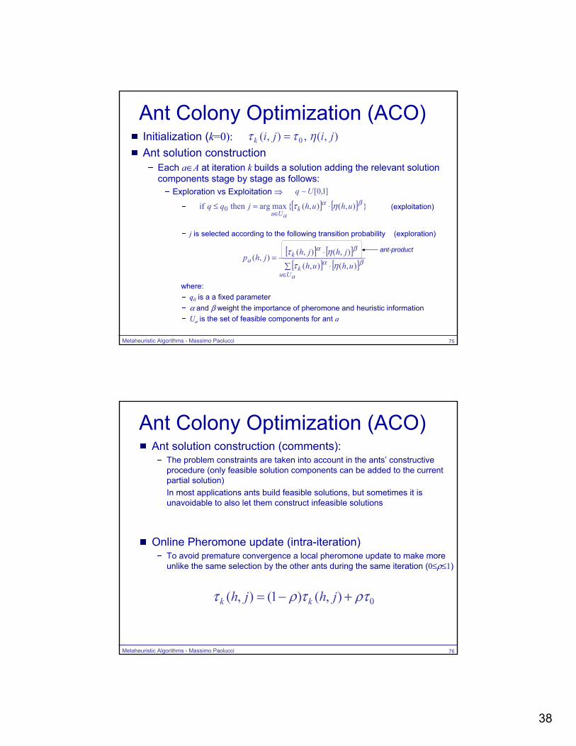
Ant Colony Optimization (ACO)Initialization (k=0):Ant solution construction
Each a∈A at iteration k builds a solution adding the relevant solution components stage by stage as follows:
Exploration vs Exploitation ⇒
(exploitation)
j is selected according to the following transition probability (exploration)
where:q0 is a a fixed parameterα and β weight the importance of pheromone and heuristic informationUa is the set of feasible components for ant a
[ ] [ ][ ] [ ]∑ ⋅
⋅=
∈ aUuk
ka
uhuhjhjh
jhp βα
βα
ητητ
),(),(),(),(
),(
),(,),( 0 jijik ηττ =
]1,0[~ Uq
[ ] [ ] }),(),({maxarg then if 0βα ητ uhuhjqq k
aUu⋅=≤
∈
ant-product
Metaheuristic Algorithms - Massimo Paolucci 76
Ant Colony Optimization (ACO)Ant solution construction (comments):
The problem constraints are taken into account in the ants’ constructive procedure (only feasible solution components can be added to the current partial solution)In most applications ants build feasible solutions, but sometimes it is unavoidable to also let them construct infeasible solutions
Online Pheromone update (intra-iteration)To avoid premature convergence a local pheromone update to make more unlike the same selection by the other ants during the same iteration (0≤ρ≤1)
0),()1(),( ρττρτ +−= jhjh kk

39
Metaheuristic Algorithms - Massimo Paolucci 77
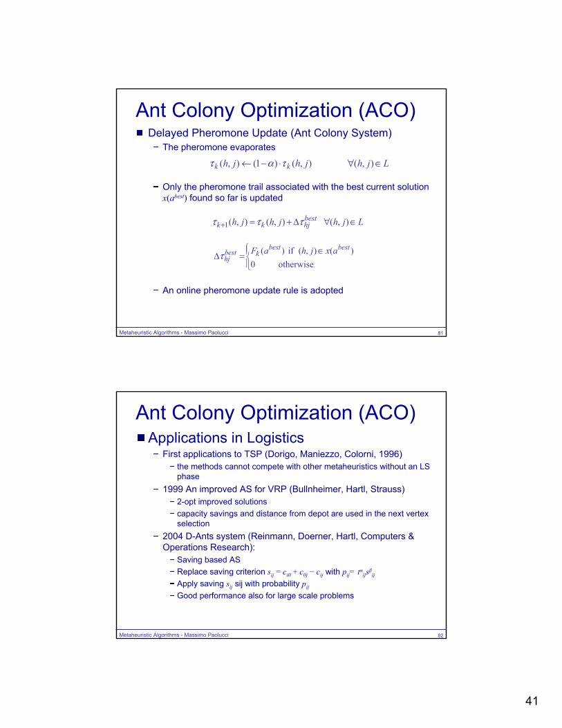
Ant Colony Optimization (ACO)Delayed Pheromone Update (DeamonAction)
After all the ants complete an iteration the pheromone trails are updated: pheromone evaporates but trails associated with qualitysolutions are reinforced
A quality function Fk(x(a)) is associated with the solution x(a) found by ant aProperty: x, x’ solutions if Z(x)<Z(x’) then F(x)≥F(x’)Simple choice: F(x(a)) = -Z(x(a))
α denotes the evaporation rate (0<α ≤1)
Alternative ant colony algorithms mainly differ for the pheromone update rule:
Ant System (AS)Max Min Ant System (MMAS)Elitist Ant System (EAS)Ant Colony System (ACS)
Metaheuristic Algorithms - Massimo Paolucci 78
Ant Colony Optimization (ACO)Delayed Pheromone Update (Ant System)
The pheromone evaporates
Every ant updates the pheromone for the components of the solution found according to solution quality (n is the number of components)
Ljhjhjh kk ∈∀⋅−← ),(),()1(),( τατ
LjhjhjhAa
ahjkk ∈∀Δ+= ∑
∈+ ),(),(),(1 τττ
⎩⎨⎧ ∈
=Δotherwise 0
)(),( if ))(( axjhaxF kkahjτ

40
Metaheuristic Algorithms - Massimo Paolucci 79
Ant Colony Optimization (ACO)Delayed Pheromone Update (Max Min Ant System)
The pheromone evaporates
Only the ant a* that found the best solution updated the pheromone trail
Ant a* may corresponds to the best ant from the beginning of the search or to the best ant in the last iterationτ(h, j)∈[τmin, τmax] to avoid null transition probability
Ljhjhjh kk ∈∀⋅−← ),(),()1(),( τατ
Ljhjhjh hjkk ∈∀Δ+=+ ),(),(),( *1 τττ
⎩⎨⎧ ∈=Δ
otherwise 0)(),( if ))(( **
* axjhaxF kkhjτ
Metaheuristic Algorithms - Massimo Paolucci 80
Ant Colony Optimization (ACO)Delayed Pheromone Update (Elitist Ant System)
The pheromone evaporates
After every ant updates the pheromone as in AS, the trail associated with the best current solution x(abest) found so far is reinforced
Ljhjhjh kk ∈∀⋅−← ),(),()1(),( τατ
Ljhjhjh besthj
Aa
ahjkk ∈∀Δ+Δ+= ∑
∈+ ),(),(),(1 ττττ
⎩⎨⎧ ∈=Δ
otherwise 0)(),( if ))(( bestbest
kbesthj
axjhaxFτ
41
Metaheuristic Algorithms - Massimo Paolucci 81
Ant Colony Optimization (ACO)Delayed Pheromone Update (Ant Colony System)
The pheromone evaporates
Only the pheromone trail associated with the best current solution x(abest) found so far is updated
An online pheromone update rule is adopted
Ljhjhjh kk ∈∀⋅−← ),(),()1(),( τατ
Ljhjhjh besthjkk ∈∀Δ+=+ ),(),(),(1 τττ
⎪⎩
⎪⎨⎧ ∈=Δ
otherwise 0)(),( if )( bestbest
kbesthj
axjhaFτ
Metaheuristic Algorithms - Massimo Paolucci 82
Ant Colony Optimization (ACO)Applications in Logistics
First applications to TSP (Dorigo, Maniezzo, Colorni, 1996)the methods cannot compete with other metaheuristics without an LS phase
1999 An improved AS for VRP (Bullnheimer, Hartl, Strauss)2-opt improved solutionscapacity savings and distance from depot are used in the next vertex selection
2004 D-Ants system (Reinmann, Doerner, Hartl, Computers & Operations Research):
Saving based ASReplace saving criterion sij = ci0 + c0j − cij with pij= tαijsβij
Apply saving sij sij with probability pij
Good performance also for large scale problems
42
Metaheuristic Algorithms - Massimo Paolucci 83
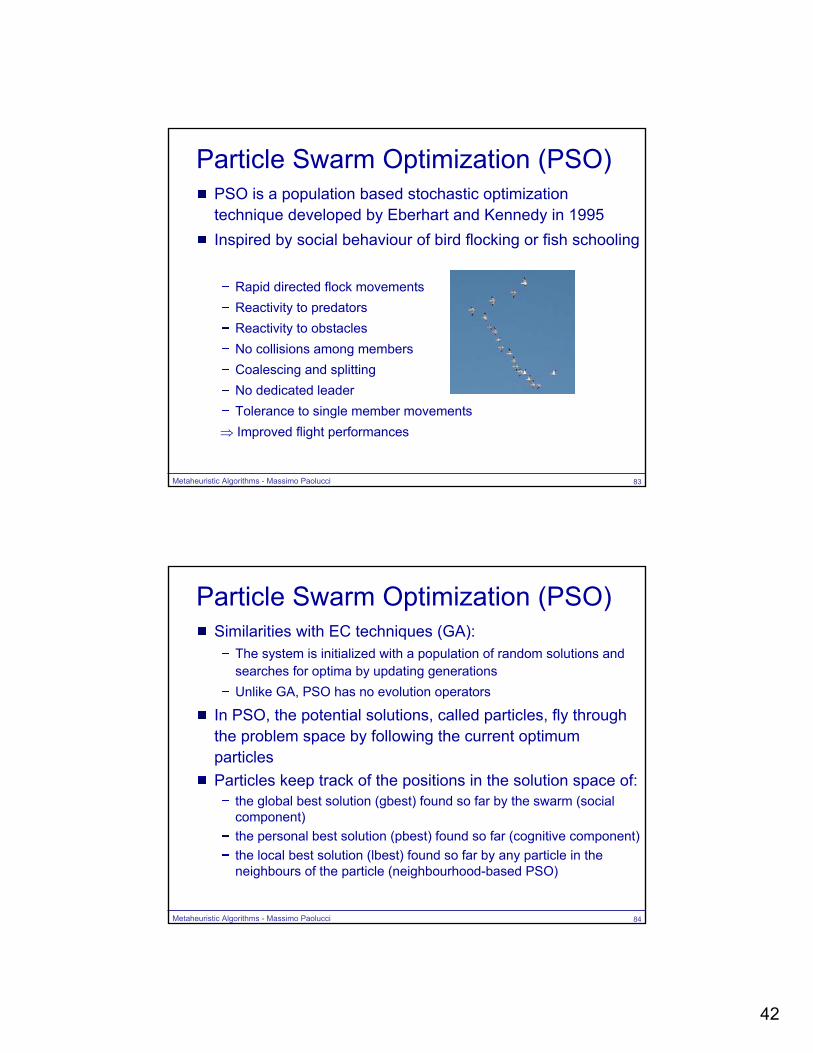
Particle Swarm Optimization (PSO)PSO is a population based stochastic optimization technique developed by Eberhart and Kennedy in 1995Inspired by social behaviour of bird flocking or fish schooling
Rapid directed flock movementsReactivity to predatorsReactivity to obstaclesNo collisions among membersCoalescing and splittingNo dedicated leaderTolerance to single member movements
⇒ Improved flight performances
Metaheuristic Algorithms - Massimo Paolucci 84
Particle Swarm Optimization (PSO)Similarities with EC techniques (GA):
The system is initialized with a population of random solutions and searches for optima by updating generationsUnlike GA, PSO has no evolution operators
In PSO, the potential solutions, called particles, fly through the problem space by following the current optimum particlesParticles keep track of the positions in the solution space of:
the global best solution (gbest) found so far by the swarm (social component)the personal best solution (pbest) found so far (cognitive component)the local best solution (lbest) found so far by any particle in the neighbours of the particle (neighbourhood-based PSO)
43
Metaheuristic Algorithms - Massimo Paolucci 85
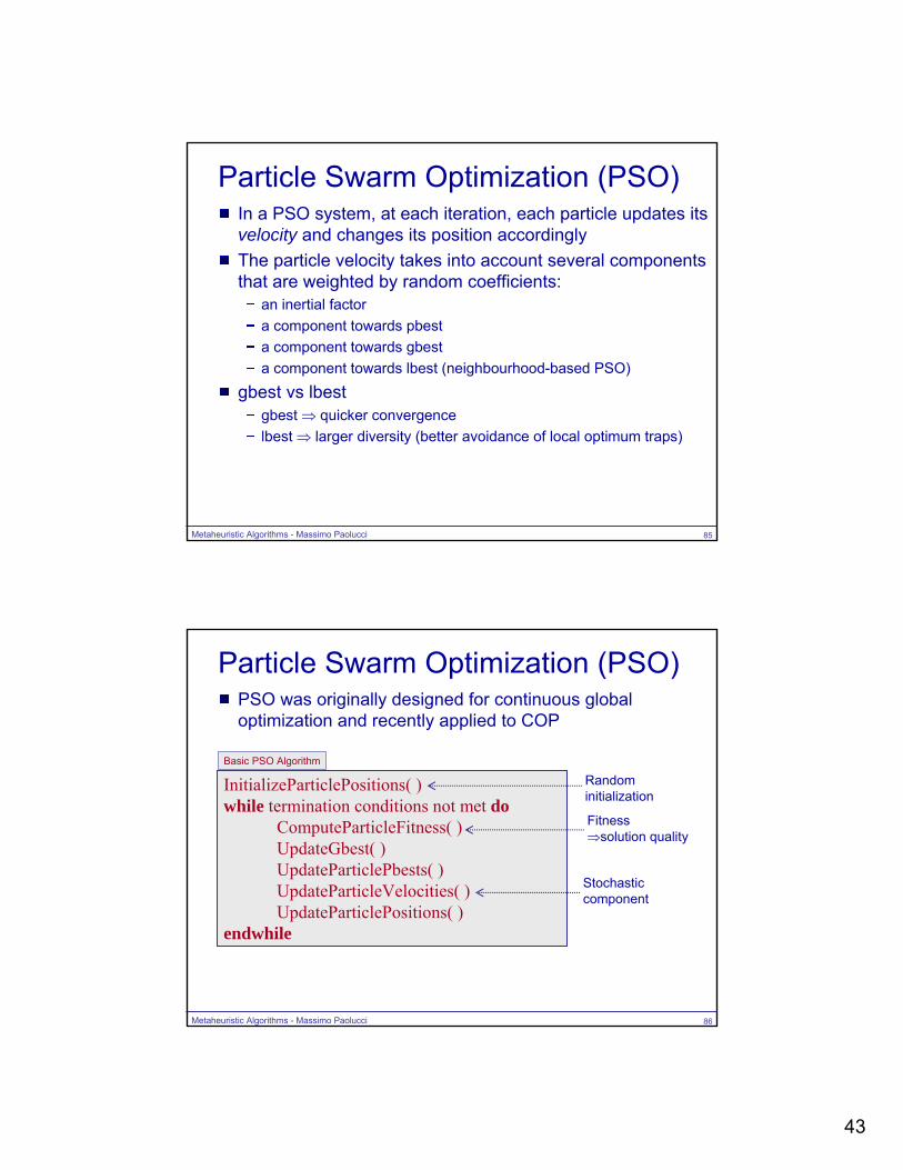
Particle Swarm Optimization (PSO)In a PSO system, at each iteration, each particle updates its velocity and changes its position accordinglyThe particle velocity takes into account several components that are weighted by random coefficients:
an inertial factora component towards pbesta component towards gbesta component towards lbest (neighbourhood-based PSO)
gbest vs lbestgbest ⇒ quicker convergencelbest ⇒ larger diversity (better avoidance of local optimum traps)
Metaheuristic Algorithms - Massimo Paolucci 86
Particle Swarm Optimization (PSO)PSO was originally designed for continuous global optimization and recently applied to COP
InitializeParticlePositions( )while termination conditions not met do
ComputeParticleFitness( )UpdateGbest( )UpdateParticlePbests( )UpdateParticleVelocities( )UpdateParticlePositions( )
endwhile
Basic PSO Algorithm
Fitness ⇒solution quality
Random initialization
Stochastic component

44
Metaheuristic Algorithms - Massimo Paolucci 87
Particle Swarm Optimization (PSO)The particle position update rule
Note that the notion of “time” is implicit ⇒ an iteration corresponds to a discrete time interval
The particle velocity update rule
Neighbourhood-based PSO
are the pbest, lbest and gbest respectively
vxx +←
)ˆ()ˆ( 2211 xxrcxxrcvv g −⋅+−⋅+⋅← ω
gl xxx ˆ,ˆ,ˆ
)ˆ()ˆ( 2211 xxrcxxrcvv l −⋅+−⋅+⋅← ω
Metaheuristic Algorithms - Massimo Paolucci 88
Particle Swarm Optimization (PSO)The particle velocity update rule (cont.)
ω is the inertial weight (real constant) c1, c2 are learning factors (real constants)
c1 weights the personal experiencec2 weights the population experience
low values ⇒ slow convergencehigh values ⇒ good solutions may be missedr1, r2 are random numbers in U[0, 1] introduced to avoid too rapid convergence
)ˆ()ˆ( 2211 xxrcxxrcvv g −⋅+−⋅+⋅← ω

45
Metaheuristic Algorithms - Massimo Paolucci 89
Particle Swarm Optimization (PSO)A pictures of particles’ movement
After a sufficient number ofiterations the particlesconverge to a goodlocal/global optimum
v
v⋅ω
)ˆ(11 xxrc −⋅)ˆ(22 xxrc g −⋅
gx̂
x
previousposition
currentposition
pbest
nextposition
Metaheuristic Algorithms - Massimo Paolucci 90
Particle Swarm Optimization (PSO)Modelling a COP ⇒ Discrete PSO require the definition of:
the correspondence between solutions and particle positions (search space)the particle fitness (objective function)the distance between a pair of particles (subtraction) ⇒ the velocitythe velocity by constant multiplication operatorthe velocity sum operatorthe move ⇒ the sum of a position with a velocity
Several models have been recently defined for Discrete PSO applied to combinatorial problems in Logistics ...

46
Metaheuristic Algorithms - Massimo Paolucci 91
Particle Swarm Optimization (PSO)Discrete PSO for TSP (Clerc, 2000)
G=(V, E) where |V|=nPosition ⇒ x=(v1,v2,...,vn-1, vn) where vi∈V and x is feasible if (vi,vi+1)∈EFitness ⇒ cost of the sequence (to be minimized)Velocity ⇒ a list of changes of positions
Example
Position plus velocity (+)⇒ apply the changes of positions in order
Example
||||,},...,1),,{( vkVjilkjiv kkkk =∈==
)5,4,2,1,3()}2,3(),1,2{()5,4,3,2,1( =+== vxvx
}5,...,1{=V )}2,3(),1,2{(=v
Metaheuristic Algorithms - Massimo Paolucci 92
Particle Swarm Optimization (PSO)Discrete PSO for TSP (Clerc, 2000)
Subtraction position minus position (-)⇒ an algorithm that produce the velocity made of the list of position changes to be applied to the second position to reach the first one
Addition velocity plus velocity (⊕)⇒ the ordered union of the lists of changes of two velocities
Opposite of a velocity (¬) ⇒ reverse the order of the changes of positions
21 xxv −=
)}5,4(),2,3(),1,2{()}5,4{()}2,3(),1,2{( 2121 =⊕== vvvv
)}1,2(),2,3{()}2,3(),1,2{( =¬= vv∅=¬⊕ vv

47
Metaheuristic Algorithms - Massimo Paolucci 93
Particle Swarm Optimization (PSO)Discrete PSO for TSP (Clerc, 2000)
Multiplication coefficient times velocity (cv) ⇒ three cases:c=0 ⇒ v = cv =∅0<c≤1 ⇒ truncate v: v’⊆v such that ||v’||=⎣c||v||⎦c>1 ⇒ c=k+c’ with k integer, 0<c’<1, then
c<0 ⇒ cv =(-c)¬v
Distance between two positions ⇒ d(x1, x2)=||x2-x1||Termination criteria:
reduction of the swarm size under a thresholdmaximum number of non-improving iterations
Possible restarting of the particles’ movement
vcvcvk
i'
1+⊕=
=
Metaheuristic Algorithms - Massimo Paolucci 94
Particle Swarm Optimization (PSO)Applications in Logistics
Discrete PSO is a quite recent approach Powerful but few published applications:
A discrete PSO method for generalized TSP problemZhi, X.H., Xing, X.L., Wang, Q.X., Zhang, L.H., Yang, X.W., Zhou, C.G., Liang, Y.C. Machine Learning and Cybernetics, 2004. Proceedings of 2004 InternationalConference, Vol 4, 2004, pp.2378 – 2383Fuzzy discrete particle swarm optimization for solving traveling salesman problemPang W, Wang K P, Zhou C G, at el., Proceedings of the 4th International Conference on Computer and Information Technology, IEEE CS Press, 2004. Hybrid discrete particle swarm optimization algorithm for capacitated vehicle routing problemCHEN Ai-ling†, YANG Gen-ke, WU Zhi-ming, Journal of Zhejiang University SCIENCE A, vol.7, 2006, pp. 607-614
48
Metaheuristic Algorithms - Massimo Paolucci 95
Neural Networks (NN)NN are networks of interconnected elementary units (weighted links)NN learn from experience by progressively adjusting the involved weights Successful applications in recognition problems and continuous control and optimizationNot competitive applications in combinatorial optimization
Metaheuristic Algorithms - Massimo Paolucci 96
Computational resultsAn excerpt from G. Laporte, Metaheuristics for the Vehicle Routing Problem: Fifteen Years of Research (www.hec.ca/chairedistributique/metaheuristics.pdf)
Regular instances:14 Christofides, Mingozzi, Toth (1979) instances (50 ≤ n ≤ 199)
Large instances:20 Golden et al. (1998) instances (200 ≤ n ≤ 480)
Comparisons with best known results (two average statistics are reported):
% over best (%ob): average deviation over bestminutes (min): CPU time in minutes
49
Metaheuristic Algorithms - Massimo Paolucci 97
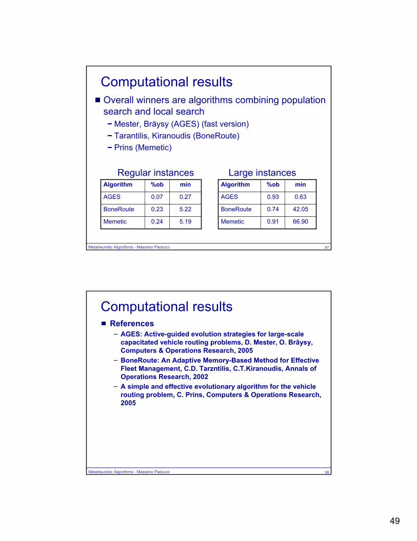
Computational resultsOverall winners are algorithms combining population search and local search
Mester, Bräysy (AGES) (fast version) Tarantilis, Kiranoudis (BoneRoute)Prins (Memetic)
5.220.23BoneRoute
5.190.24Memetic
0.270.07AGES
min%obAlgorithm
Regular instances
42.050.74BoneRoute
66.900.91Memetic
0.630.93AGES
min%obAlgorithm
Large instances
Metaheuristic Algorithms - Massimo Paolucci 98
Computational resultsReferences
AGES: Active-guided evolution strategies for large-scale capacitated vehicle routing problems, D. Mester, O. Bräysy, Computers & Operations Research, 2005BoneRoute: An Adaptive Memory-Based Method for Effective Fleet Management, C.D. Tarzntilis, C.T.Kiranoudis, Annals of Operations Research, 2002A simple and effective evolutionary algorithm for the vehicle routing problem, C. Prins, Computers & Operations Research, 2005

50
Metaheuristic Algorithms - Massimo Paolucci 99
BibliographyMetaheuristics Network (http://www.metaheuristics.org)R.K. Ahuja, Ö. Ergun, J.B. Orlin, A. P. Punnen, “A survey of very large-scaleneighborhood search tecniques”, Discrete Applied Mathematics 123 (2002) 75-102.P. Hansen, N. Mladenović, “Variable neighborhood search: Principle and applications”, European Journal of Operational Research, 130 (2001) 449-467.Bonabeau E, Dorigo M and Theraulaz G (1999) Swarm Intelligence: From Natural to Artifcial Systems. New York, NY: Oxford University PressKennedy J and Eberhart R (2001) Swarm intelligence. Morgan Kaufmann Publishers, Inc., San Francisco, CA.Pang W, Wang K P, Zhou C G, at el. (2004) Fuzzy discrete particle swarm optimization for solving traveling salesman problem. Proceedings of the 4th International Conference on Computer and Information Technology, IEEE CS Press.P. Toth and D. Vigo, The Vehicle Routing Problem, SIAM Monographs on Discrete Mathematics and Applications, Philadelphia, 2002.M. Dorigo, V. Maniezzo, A. Colorni.“The Ant System: Optimization by a colony of cooperating agents”, IEEE Transactions on Systems, Man, and Cybernetics–Part B, Vol.26, 1996, pp.1-13