PANG InformationHigherOrderBSDerivative

Additional Information in Higher Order Derivatives

of the Black-Scholes formula

Department of Economics Supervisor: Birger NilssonBachelor's thesis, Aug 09 Author: Jenny Pang

Abstract

Volatility smile arising from the Black-Scholes model is a long studied subject in option

pricing theory. By analysing higher order derivatives of the model, I hope to put another

perspective to the problem. Accoridng to a study on the American S&P 500 future options,

about 90% of the risks of holding an option in five days can be removed by using higher order

derivatives of Black-Scholes. The objective of this thesis is to investigate whether or not the

price changes of Swedish OMX-index options follow the Taylor expansion of Black-Scholes.

The method used here is to compare the observed option price changes after five holding days

with the price changes predicted by first, second and third order Taylor serie.

The findings and conclusions of this study can be summarised as follow: 1. The mean of

prediction errors increases as higher order derivatives are used to predict the price changes,

suggesting that the OMX-index options do not follow Taylor expansion of Black-Scholes. 2.

As the standard deviation of the prediction errors is decreasing when orders of derivatives in

use increase, I conclude that there is additional information in the second and third order

derivatives of Black-Scholes. 3. Increasing maturity leads to better predictions, suggesting

that the Black-Scholes differential equation is better at describing the movement of long

maturity options.

Keywords: Greeks, Black-Scholes, Higher order derivatives, Taylor expansion.

Acknownledgement

I would like to propose special thanks to those who have helped me on this thesis; Birger

Nilsson, Ignacio Lujan, Peter Gustafsson, and last but not least, Yuesheng Jin.

Table of contents

I. BackgroundBasics about options ....................................................................................1Black-Scholes – theory and practice ...........................................................2Volatility smile ............................................................................................ 4Criticism and justification ...........................................................................5

II. ProblemIssues and former study ...............................................................................7

III. DataIssues of data ...............................................................................................10Sample framing ........................................................................................... 11

IV. Mathematics & FormulaeBlack-Scholes ..............................................................................................13The five greeks ............................................................................................13Higher order derivatives ..............................................................................14Taylor expansion ......................................................................................... 15The test model .............................................................................................16

V. ProcedureData management ........................................................................................18Calculations .................................................................................................18Making samples .......................................................................................... 19Analysis .......................................................................................................19

VI. AnalysisConclusion .................................................................................................. 24Discussion ................................................................................................... 25

Endnotes ..................................................................................................................26References ...............................................................................................................27Appendix:

TablesFormulaeProgrammes

I. Background

The Black-Scholes model is the most famous model for option pricing. The elegance of the

model lies in that it only uses a few parameters, the calculation is simple, and it creates a

perfect hedge to the underlying asset. However, it is also the most debated model. In spite of

its elegance it also has deficiencies. One of the variables in the model, volatility, which is

assumed to be constant for all strikes and maturities, appears to be different when observing

the market. The market prices implies higher volatility for low strikes and lower volatility for

high strikes. It forms a pattern known as the volatility smile. Numerous research have studied

this phenomenon, some researchers conclude that the volatility smile is merely a post crash

fear caused by hedging pressure, which is not seen before 1987. While others have proposed a

modified Black-Scholes model with jump diffusion or stochastic volatility incorporated, or

both, in order to fit the market better. An analysis of higher order derivatives of the Black-

Scholes will put another perspective to this contradiction. The objective of this thesis is to

investigate whether or not the price change of the Swedish OMX index option will follow a

Taylor expansion of the Black-Scholes model.

Basics about options

Option is a contract between a buyer and a seller in which the buyer has the right, but not the

obligation, to buy or sell a certain asset (called the underlying asset) to a predetermined price

(called strike price), in a predetermined time in the future (time-to-maturity). If the buyer

(long position) chooses to exercise the right, the seller (short position) is obliged to sell or buy

the asset at the agreed price. Call options gives the right to buy whereas put option gives the

right to sell.

The concept of option is known to be used since ancient time. However the first well-known

option market was established in Holland in the early 17th century, trading tulips. The purpose

of options served as security for producers and merchandisers at the beginning, but soon the

1

market had attracted many speculaters. This incidence, known as the tulip mania, is the first

recorded economic bubble in history[1].

Today it is possible to trade options on all kinds of assets, stocks, foreign exchange,

commodities, energy etc. The variety of option styles is even more substantial. There are

standardised options like European option, American option and Asian option. A standardised

option can be traded in a market to a bid-ask spread and supposely free from arbitrage.

Options that are not standardised are exotic options, barrier options, shout options, rainbow

option, binary option, power options to name a few. Exotic options can usually not be found

in a market but are tailor made and traded over the counter. Usually there are no standardised

models for pricing different types of exotic options. Depending on the contract, pricing exotic

options can be very complex.

The option style discussed here is European options. At the expiration day if the price of the

underlying asset exceeds the strike price of a call option, the buyer receives the difference.

However if the price of the underlying asset is below the strike price, the buyer loses the

premium he paid for the option. It is the same principle for an European put option.

The Black-Scholes model – theory and practice

The Black-Scholes model was first published in 1973 and it's impact on option pricing is

evolutionary. It is believed that the Black-Scholes model laid the foundation for the rapid

growth of markets for derivatives since publishing[2]. The beginning of today's modern option

pricing theory dates back to the early 20th century. A French mathematician, Louis Bachelier,

offered the earliest known analytic valuation for options using stochastic process, now known

as the Brownian motion. This is presented in his Ph.d. dissertation, “The Theory of

Speculation”[3][4]. Since Bachelier, the model has been developed and improved by later

researchers. One of them is James Boness, who derived a formula which laid the foundation

for today's Black-Scholes. All predecessors of Black-Scholes suffered from one shortcoming,

the risk premium were not dealt with in a proper way. To estimate the risk premium, one had

2

to know or make assumptions on the invester's risk preferences. But Black and Scholes found

a way to derive so that the risk premium was removed in the formula. This does not mean that

the risk premium has disappeared, in fact, it is already included in the stock price[5]. This

improvement earned Fisher Black, Myron Scholes and Robert Merton the Economy price in

honour of Nobel 1997.

The central idea of Black-Scholes (here after BS) is dynamic delta hedging. By rebalancing a

portfolio consisting of bonds and the underlying asset, it is possible to replicate the value of

the option. The proportion of the underlying asset in the portfolio is depended on the delta of

the option. A portfolio that is delta neutral is relatively insensitive to change in the price of the

underlying asset.

While the academics praise the BS-models, it is not as appreciated or maybe even used by the

practitioners*[6]. To be able to remove the risks related to the underlying asset, continuous

hedging (rebalancing portfolio with infinitly small time intervals) is required. As this is not

implementable in reality, static hedging (rebalacing the portfolio once in a while) will creat

risks. If the time intervall between each rebalancing is large, then movement of the underlying

asset creates risks. In contrast, if the time intervall between each rebalancing is small,

transaction fees quickly adds up. Further more it is evident that some of the assumptions made

by the BS do not conform to reality. The assumptions used to derive the Black-Scholes-

Merton differential equation[7]:

1. The stock price follows a geometric Brownien Motion with constant drift and

volatility.

2. There are no restrictions on short selling.

3. There are no transaction costs or taxes. All securities are perfectly divisible.

4. There are no dividends during the life of the derivative.

5. The are no riskless arbitrage opportunities.

6. The riskless rate is constant during the life of the option.

* Practitioners here refers to traders operating on option markets.

3

The first assumption is sometimes formulated as stock price has log normal proporties. Many

studies have tried to recover the empirical stock price distribution. Often the empirical

distribution is more skewed to the left than log normal distribution[8]. Also, the volatility of the

stock is not constant over the option's lifetime. As new informations arriving to the market

continuously, the market's expectation on the asset's volatility will change. This risk is not

included in the BS-model.

The third assumption is conditions of an ideal world. While in the real world there are

transaction costs and taxes, and securities are not perfectly divisible. These are the

technicalities that prevent dynamic replication.

The last assumption, riskfree rate is a stochastic variable and not constant. It is possible to

hedge the riskless rate though. There are other option pricing models that relaxis this

assumption.

The volatility smile

All parameters in the BS-formula can be observed, all exept for one, the stock price volatility.

The implied volatility can be obtained by substituting all parameters, stock price, strike price,

riskfree interest rate, time to maturity, and the market price of the option into the BS formula.

This is the volatility estimated by the market. When plotting implied volatility of the options

against strikes and maturities, it appears not to be constant, as the BS-model assumes. For

equity options, the implied volatility is higher for low strikes and diminishes as the strike

compounds[9][10]. It is often refered to as the volatility smirk in the literature. For foreign

exchange options, the implied volatility forms a smile pattern when plotted against the strikes.

Term structure of volatility refers to that the smile is more pronounced closer to the maturity.

Over the years the research about the volatility smile has been extensive but so far it is a

debate without an solution. Some researchers claim that the smile found in stock options is

caused by hedging pressure, crash-o-phobia after the stock market crash in 1987[11]. While

some others argue that BS underestimates extreme events which the market have priced.

4

Criticism and justification

If the BS-model is correct, one could theoretically profit from the market abnormality.

Literature testing market inefficiencies are extensive, for example Black and Scholes(1972),

Galai(1977), Chiras and Manaster(1978) and Ederington and Guan(2002). The general

conclusion is without transacting fee, there are substantial winnings. But once transaction fee

is included, there are no arbitrage opportunities. Ederington and Guan (2002) even found that

the true smile is some what flatter than the observed smile but it is not completely flat as

assumed in the BS*. In another paper Ederington and Guan (2007: Higher Order Greeks)

showed that the 2:nd and 3:rd order derivatives of BS are quite good in explaining price

changes of the S&P 500 future options, 90% of the risks are removed when higher order

derivatives are considerated. This justifies the BS-model. Baksi, Cao and Chen (1995)

compared the empirical performance of BS and other alternative models that allowed

stochastic volatility, or jump diffusion, or stochastic interest rate. They tested the models'

performance based on three yardsticks, internal consistancy of implied parameters (implied

volatility), the out of sample data, and the hedging ability. Overall, BS had the worst

performance in all three categories whereas stochastic volatility model had the best

performance. Jump-diffusion added to stochastic volatility improved the fit of the short

maturity options. They also found that delta hedging BS consistantly resulted in overhedging.

According to Haug and Taleb (2008), Nelson (1904) pointed out that delta hedging worked

better in theory than in practice. Delta hedging is not a new idea coming with BS, it wasn't

used because it wasn't considered as a good hedging strategy.

Analysing Taylor expansion of BS is one way to evaluate the model. Based on the idea of

Ederington and Guan (2007), I will do a study on Swedish OMX-index options. The thesis

have the following disposition; in section two the issues arising from implemeting the study is

discussed. Followed by an analysis of data in section three. In section four the mathematics

* The authors meant that the true smile is the part of the smile one can not profit from even before transaction costs. The true smile should be due to model deficiencies. Whereas a part of the observed smile is due to market inefficiency and one can profit from it before transaction costs.

5

and formulae are described. In the next section programming process is described in detail. In

the last section the results are analysed, followed by a conclusion and a discussion.

6

II. Problem

One way to find out whether or not BS is an adequate model for options pricing is to analyse

it's power to predict option's price changes. Traditionally only the four first order derivatives

and a second order derivative, gamma, are mentioned in the literature. Ederington and Guan

are the first and the only ones to publish a study of all second and third order derivatives of

BS. Could the second and third order derivatives of the BS-model contain useful information

as well? Does the importance of the additional information from the derivatives depend on the

option's strike or maturity? To be able to answer these question I will compare the observed

option price change with the price changes predicted by first, second and third order Taylor

expansion of BS.

Issues and former study

In Higher Order Greeks the authors concluded that the option price changes follow the Taylor

expansion (here after T-E) of BS. This conclusion could be wrongly interpreted since their

result suggests, based on a study of a prespecified holding period, to which they set to five

days, most of the option price changes can be explained by combining first, second and third

order derivatives of BS. However, nothing is known about when the holding period is less

than five days nor when it is more than five days. To verify that option price changes follow

T-E of BS, studying different holding days is nessesary. If the prediction of option price

changes is more precise when holding period is short and less precise as holding period

extends, then we can conclude that option prices follow T-E of BS and BS could be an

adequate option pricing model. But if the prediction for shorter holding period is less accurate

or equally precise as predictions for longer holding period, in both cases the price changes do

not follow a T-E of BS. Since nothing is known about the prediction ability for other holding

days, we cannot come to any conclusion. However, the author's motivation for setting holding

period to five days is that it is long enough to eliminate bid-ask spread and short enough for

7

the derivatives to remain relatively unchanged. Doing a study on different holding days is

prefered, but since the thesis will become too extensive, I limited this thesis to study only five

days.

The second issue is the choice of volatility. Since the constant volatility property is violated,

the choice of volatility is not obvious. The authors of Higher Order Greeks have chosen to use

an average of five implied volatilities, volatilities from the strike above and below the option

concerned, and the opposite option type with the three strikes closest to the option. For

example if we are calculating an averaged volatility for a put option with strike 800, we take

an average of implied volatilities from put with strikes 810 and 790, calls with strikes 810,

800 and 790. Motivation for this method is that the observed volatility increase or decrease

arising from bid-ask spread will be eliminated by averaging the implied volatilities. This is a

good idea, but, if the authors use implied volatility, which is already a deviation from the BS-

model, whatever result they will get will not justify the BS-model but a modified BS-model.

Second, if using an average implied volatility which most likely will differ from the implied

volatility of the option concerned, we will derive a new call or put price when putting back

the average implied volatility into the BS-model. When calculating the observed price change

of the option, should we use the observed prices or the option prices derived from the

averaged implied volatility? This study will focus on how well the BS model fits the market.

Since the bid-ask spread is a reality, I will not attempt to eliminate or compromise it.

The last issue concerns framing the subsamples, i.e. dividing the data into maturity and strike

subsamples. Refering to Higher Order Greeks again, their data was divided into two maturity

samples and each maturity sample had five strike samples. The division of maturity samples,

one short maturity sample with options within 4-12 weeks to maturity, and one long maturity

sample, with options within 13-26 weeks to maturity, is due to the S&P 500 futures having

maturity four times a year. Option from the long maturity sample uses an S&P future different

from options of the short maturity sample. The strike samples are respectivly one ITM

sample, one ATM sample and three OTM samples. There are three OTM-samples and only

8

one ITM-sample because trading in OTMs is much heavier than trading in ITMs. The samples

here will be framed in a simular way as in Higher Order Greeks. The motivation for the

framing needs data analysis and is therefore discussed in the next section instead.

9

III. Data

The options chosen to be examined here are options on index of Swedish exchange,

OMXS30. The analysing period is 2001-2006. The reason for the choice of the underlying

asset is firstly, I want to evaluate BS-model for equity. Secondly, the options traded most

frequently on the exchange are prefered. I have collected the closing prices for all options on

OMXS30 during the selected period. Closing quotes of the index and daily rate of the

STIBOR (riskfree rate) are collected from the homepage of OMX[12] respectively from the

homepage of the Swedish Central Bank[13].

Issues of data

Closing quotations are not the ideal data to use since they can give missleading information.

By analysing the daily highs and lows of OMXS30, I found that during the period of

2001-2006, the range of OMXS30 could be up to 12% a day. For example if OMX is 1000kr

some day and the range that day is 12%, then at least 6 strikes could be ATM that day. When

options are categorised according to strikes, an ITM-option traded earlier that day could be

treated as an OTM-option according to closing quote information. If tick data is used instead,

it is then possible to match the option's moneyness with the OMX quote at the time the option

is executed. But since neither the exchange nor other public sources provide tick data, I can

only use closing quotes here. Since the mismatching problem will only trouble options that

are thinly traded, I will only use option strikes that are with certainty traded until closing.

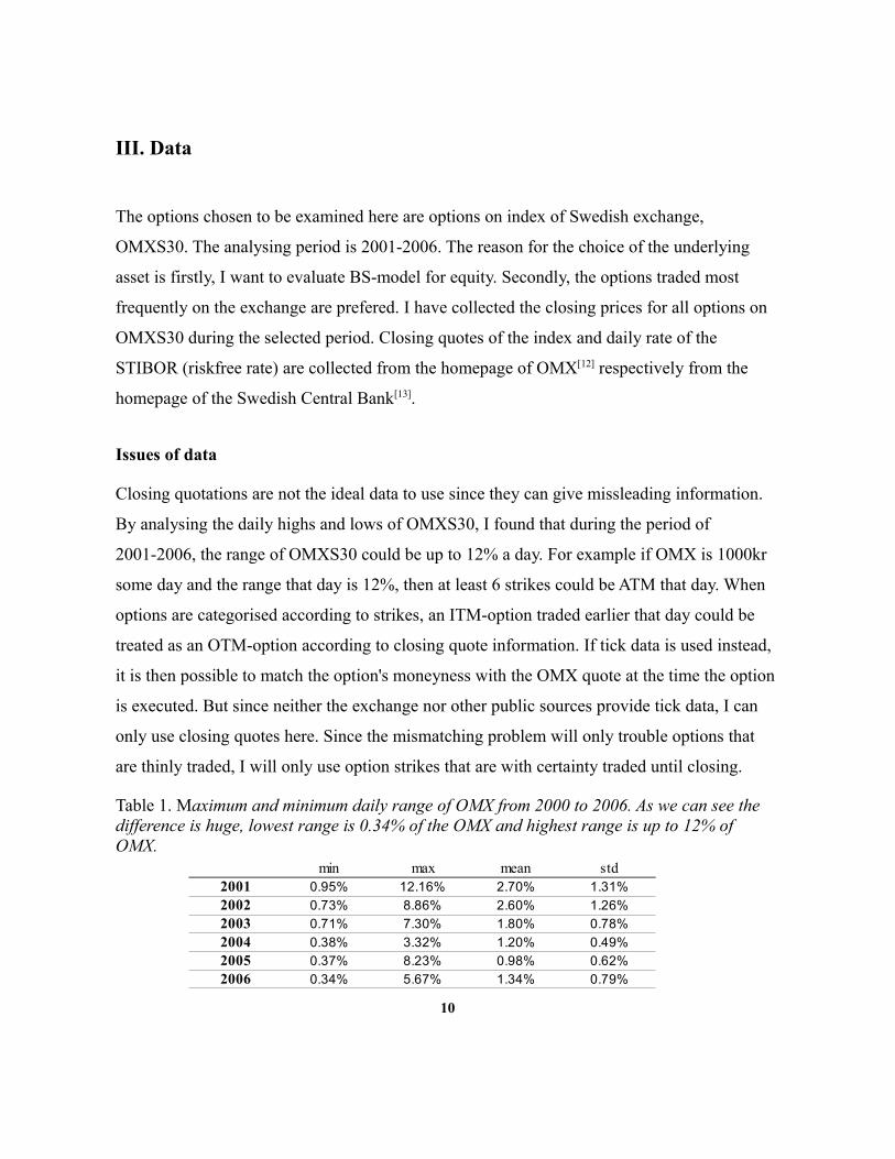
Table 1. Maximum and minimum daily range of OMX from 2000 to 2006. As we can see the difference is huge, lowest range is 0.34% of the OMX and highest range is up to 12% of OMX.

10

min max mean std2001 0.95% 12.16% 2.70% 1.31%2002 0.73% 8.86% 2.60% 1.26%2003 0.71% 7.30% 1.80% 0.78%2004 0.38% 3.32% 1.20% 0.49%2005 0.37% 8.23% 0.98% 0.62%2006 0.34% 5.67% 1.34% 0.79%

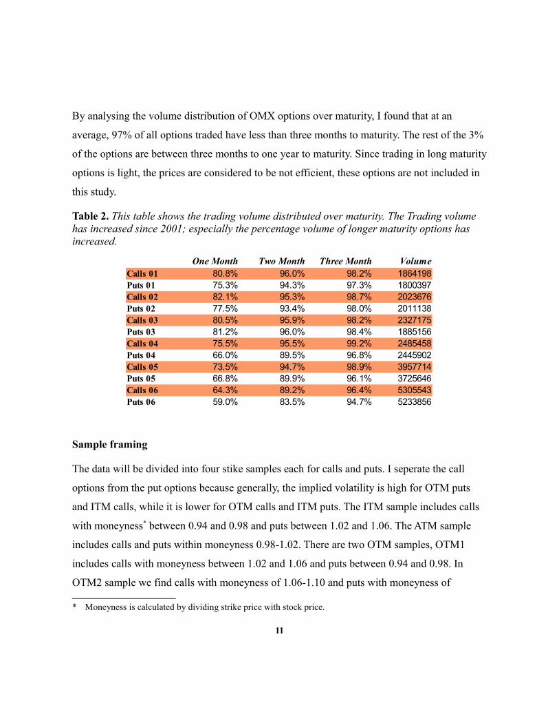
By analysing the volume distribution of OMX options over maturity, I found that at an

average, 97% of all options traded have less than three months to maturity. The rest of the 3%

of the options are between three months to one year to maturity. Since trading in long maturity

options is light, the prices are considered to be not efficient, these options are not included in

this study.

Table 2. This table shows the trading volume distributed over maturity. The Trading volume has increased since 2001; especially the percentage volume of longer maturity options has increased.

Sample framing

The data will be divided into four stike samples each for calls and puts. I seperate the call

options from the put options because generally, the implied volatility is high for OTM puts

and ITM calls, while it is lower for OTM calls and ITM puts. The ITM sample includes calls

with moneyness* between 0.94 and 0.98 and puts between 1.02 and 1.06. The ATM sample

includes calls and puts within moneyness 0.98-1.02. There are two OTM samples, OTM1

includes calls with moneyness between 1.02 and 1.06 and puts between 0.94 and 0.98. In

OTM2 sample we find calls with moneyness of 1.06-1.10 and puts with moneyness of

* Moneyness is calculated by dividing strike price with stock price.

11

One Month Two Month Three Month VolumeCalls 01 80.8% 96.0% 98.2% 1864198Puts 01 75.3% 94.3% 97.3% 1800397Calls 02 82.1% 95.3% 98.7% 2023676Puts 02 77.5% 93.4% 98.0% 2011138Calls 03 80.5% 95.9% 98.2% 2327175Puts 03 81.2% 96.0% 98.4% 1885156Calls 04 75.5% 95.5% 99.2% 2485458Puts 04 66.0% 89.5% 96.8% 2445902Calls 05 73.5% 94.7% 98.9% 3957714Puts 05 66.8% 89.9% 96.1% 3725646Calls 06 64.3% 89.2% 96.4% 5305543Puts 06 59.0% 83.5% 94.7% 5233856

0.90-0.94. Other data will be excluded from this study, since the options outside this range are

considered thinly traded. The moneyness calculated from options that are thinly traded are not

always reliable.

Options with maturities longer than 13 weeks are not included in this study. The maturity-

samples will be divided on a weekly bases. For example the sample that has 13 weeks to

maturity includes options that have 61 to 65 business days to maturity. (which means it uses

option prices from same the week as the option expires. Usually it is not recommended to use

this data since the options prices can be manipulated. But I have used it in my study anyway

and as we can see the data looks a bit strange.)

12

IV. Mathematics and formulae

Black-Scholes

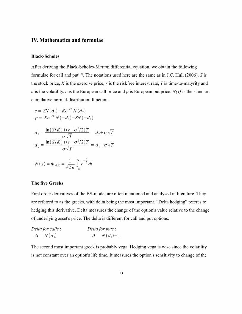
After deriving the Black-Scholes-Merton differential equation, we obtain the following

formulae for call and put[14]. The notations used here are the same as in J.C. Hull (2006). S is

the stock price, K is the exercise price, r is the riskfree interest rate, T is time-to-matyrity and

σ is the volatility. c is the European call price and p is European put price. N(x) is the standard

cumulative normal-distribution function.

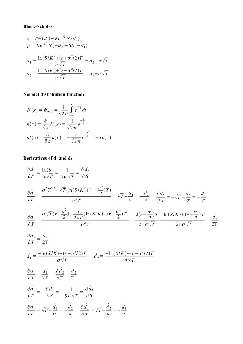
c = SN d 1−Ke−rT N d 2p = Ke−rT N −d 2−SN −d 1

d 1 =ln S /K r 2/2T

T= d 2 T

d 2 =lnS /K r−2/2T

T= d 1−T

N x = 0,1 =1

2∫−∞x

e− t2

2 dt

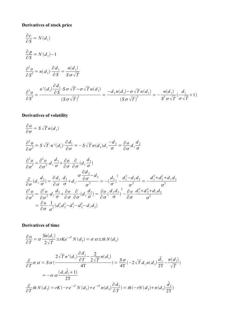
The five Greeks

First order derivatives of the BS-model are often mentioned and analysed in literature. They

are referred to as the greeks, with delta being the most important. “Delta hedging” referes to

hedging this derivative. Delta measures the change of the option's value relative to the change

of underlying asset's price. The delta is different for call and put options.

Delta for calls : Delta for puts : = N d 1 = N d 1−1

The second most important greek is probably vega. Hedging vega is wise since the volatility

is not constant over an option's life time. It measures the option's sensitivity to change of the

13

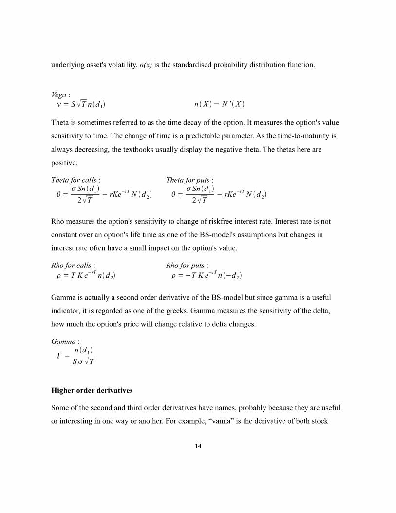
underlying asset's volatility. n(x) is the standardised probability distribution function.

Vega : = S T nd 1 n X = N ' X

Theta is sometimes referred to as the time decay of the option. It measures the option's value

sensitivity to time. The change of time is a predictable parameter. As the time-to-maturity is

always decreasing, the textbooks usually display the negative theta. The thetas here are

positive.

Theta for calls : Theta for puts :

= Sn d 1

2T rKe−rT N d 2 =

Sn d 12T

− rKe−rT N d 2

Rho measures the option's sensitivity to change of riskfree interest rate. Interest rate is not

constant over an option's life time as one of the BS-model's assumptions but changes in

interest rate often have a small impact on the option's value.

Rho for calls : Rho for puts : = T K e−rT nd 2 =−T K e−rT n −d 2

Gamma is actually a second order derivative of the BS-model but since gamma is a useful

indicator, it is regarded as one of the greeks. Gamma measures the sensitivity of the delta,

how much the option's price will change relative to delta changes.

Gamma :

=n d 1S T

Higher order derivatives

Some of the second and third order derivatives have names, probably because they are useful

or interesting in one way or another. For example, “vanna” is the derivative of both stock

14

price and volatility, and “color” is the derivative of gamma and time. There are fifteen second

and third order derivatives in total, excluding gamma and all derivatives of rho. The

derivatives of rho are not included here due to their impact on option price changes are very

small[15].The formulae are shown in Appendix Formulae. Since not all of the derivatives have

names I will present the derivatives with symbols.

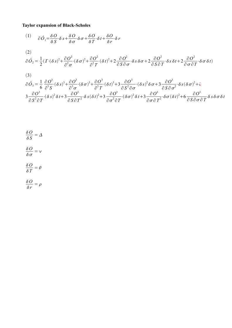
Taylor expansion

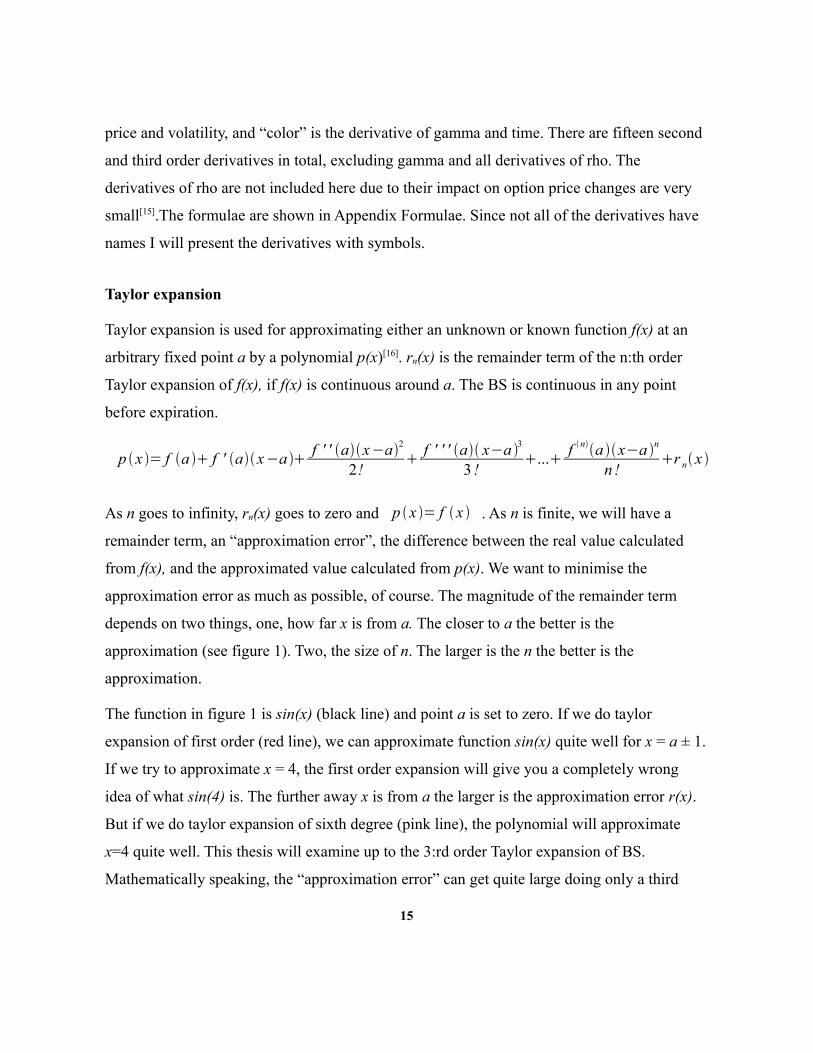
Taylor expansion is used for approximating either an unknown or known function f(x) at an

arbitrary fixed point a by a polynomial p(x)[16]. rn(x) is the remainder term of the n:th order

Taylor expansion of f(x), if f(x) is continuous around a. The BS is continuous in any point

before expiration.

p x = f a f ' ax−a f ' ' ax−a2

2! f ' ' ' a x−a 3

3 !... f na x−a n

n!r nx

As n goes to infinity, rn(x) goes to zero and p x = f x . As n is finite, we will have a

remainder term, an “approximation error”, the difference between the real value calculated

from f(x), and the approximated value calculated from p(x). We want to minimise the

approximation error as much as possible, of course. The magnitude of the remainder term

depends on two things, one, how far x is from a. The closer to a the better is the

approximation (see figure 1). Two, the size of n. The larger is the n the better is the

approximation.

The function in figure 1 is sin(x) (black line) and point a is set to zero. If we do taylor

expansion of first order (red line), we can approximate function sin(x) quite well for x = a ± 1.

If we try to approximate x = 4, the first order expansion will give you a completely wrong

idea of what sin(4) is. The further away x is from a the larger is the approximation error r(x).

But if we do taylor expansion of sixth degree (pink line), the polynomial will approximate

x=4 quite well. This thesis will examine up to the 3:rd order Taylor expansion of BS.

Mathematically speaking, the “approximation error” can get quite large doing only a third

15

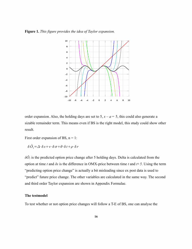
Figure 1. This figure provides the idea of Taylor expansion.

order expansion. Also, the holding days are set to 5, x – a = 5, this could also generate a

sizable remainder term. This means even if BS is the right model, this study could show other

result.

First order expansion of BS, n = 1:

O1=⋅ s⋅⋅ t⋅ r

δÔ1 is the predicted option price change after 5 holding days. Delta is calculated from the

option at time t and δs is the difference in OMX-price between time t and t+5. Using the term

“predicting option price change” is actually a bit misleading since ex post data is used to

“predict” future price change. The other variables are calculated in the same way. The second

and third order Taylor expansion are shown in Appendix Formulae.

The testmodel

To test whether or not option price changes will follow a T-E of BS, one can analyse the

16

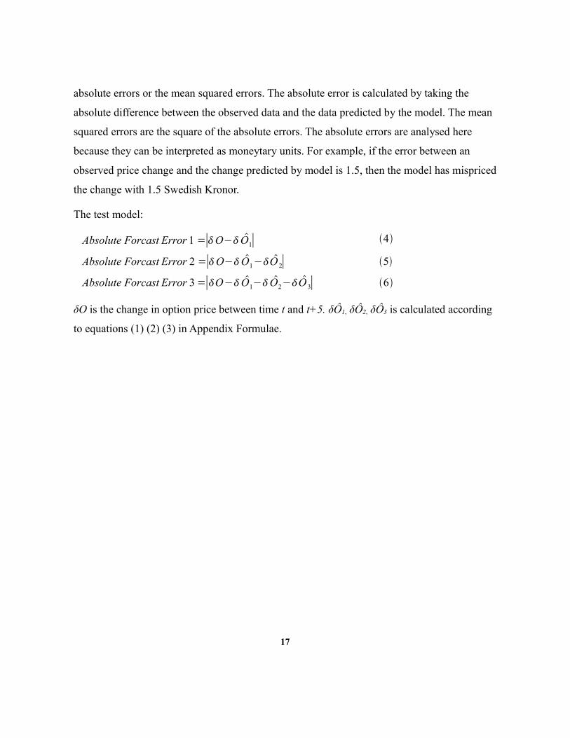
absolute errors or the mean squared errors. The absolute error is calculated by taking the

absolute difference between the observed data and the data predicted by the model. The mean

squared errors are the square of the absolute errors. The absolute errors are analysed here

because they can be interpreted as moneytary units. For example, if the error between an

observed price change and the change predicted by model is 1.5, then the model has mispriced

the change with 1.5 Swedish Kronor.

The test model:

Absolute Forcast Error 1 =∣O− O1∣ 4

Absolute Forcast Error 2 =∣O− O1− O 2∣ 5

Absolute Forcast Error 3=∣O− O1− O2− O 3∣ 6

δO is the change in option price between time t and t+5. δÔ1, δÔ2, δÔ3 is calculated according

to equations (1) (2) (3) in Appendix Formulae.

17

V. Procedure

To be able to handle the massive option data and make computations efficient, programming

is inevitable. I choose to use MatLab because it is powerful for calculations and matrix

operations. The programming is carried out in 4 steps, the first step is to handle the collected

data, to read it into Matlab, sorting the data and make them easy to manage. The second step

is to perform calculations of implied volatilities, moneyness and all derivatives of the options.

The third step is to find data with specific attributes, for example, to find all ATM call options

with 10-15 days to maturity. After, the observed option price change and the AFEs (absolute

forecast errors from equations (4)(5)(6)) are calculated for all samples. At the fourth and final

step the means and standard deviations of observed price change and AFEs are calculated and

put together in the Appendix Tables. The rest of the programmes are made to help analysing

the results.

Data management

The option data collected from OMX are in text format and one file contains data from one

month. All options that were listed on OMX each day. Program extractdata reads the text files

into Matlab and sorts the options that are not OMX options or were not traded. The read-in

data is then processed in the next program sortera, where the option data is sorted by their

names. For example an option is named OMXS305A700, the program finds all options with

this name in the monthly data and save the date it was traded and the closing prices. In

october 2004 the OMX options changed names from OMX/year/month/type/strike to

OMXS30/year/month/type/strike, hence the treatment of option data from 2004-2005 required

special care.

Calculations

To proceed with calculations of derivatives we must first find implied volatilities for all

18

options. I use a built-in Matlab function, blsimpvol, to obtain implied volatilities. The built-in

function was able to solve most but not all implied volatilities. The reason why some implied

volatilities could not be obtained is unknown. The problem could be the data or the built-in

function. After, moneyness is computed for all options in program moneyness. Before

proceeding to calculations of derivatives, options with invalid implied volatility had to be

deleted first in invimpvol. I choose not to use options with implied volatility higher than 45%

because high volatilities are more likely to be caused by bid-ask spread or non-syncronised

data rather than estimated by the market. These data are also deleted in invimpvol.

Making subsamples

The main program at this step is run, it is mainly for getting datas and sending variables

between the functions sampcol and forcaster. The parameters are set in run, the strikes,

maturity and holding period. Sampcol finds the options that fit the parameters, and if it finds

the very same option traded 5 days later, it saves the option's name and traded dates in a table.

For example we are looking for all ATM calls that expires in March 2003 and have 3 weeks to

maturity. The program first looks for the date of expiration, then it finds the dates between

15-11 days before expiration. The matlab class fints is used to find whether or not an option is

traded in those specified days. The programme forcaster starts with converting all option

information (including implied volatilities and all derivatives) from class struct to class fints.

By using fints, it is easy to calculate δs, δσ, δt, δr, which are needed for calculating δO, δÔ1,

δÔ2 and δÔ3.

Analysis

At the first attempt, I intend to analyse the data annually, considering the fact that market's up

and down trends or the variation in volatility could have effect on prediction abilities.

However I realised it would be too much data to be analyse. Instead, I put together the data of

six years to be one sample. Even by doing this way, a total of 16 tables were resulted, let alone

19

how many tables I would have had if the data are analysed annually. The programme

gruppering begins with putting together the data of six years, following by calculating the

AFEs. Analys calculates the mean and standard deviation for all AFEs. After the first

observation, analys was extended to carry out some linear regressions. Analys put the data

together in a table while linreg is the programme actually perfoming the linear regression[17].

The programme acrosstrikes tests the relation between moneyness and mean of AFEs and the

relation between moneyness and standard deviation of AFEs. Programme lilliefors makes

lilliefors test for all samples and puts the result in tables 17-18. More details about the test and

why it is used is explained in the next section. I used the built-in Matlab function, lillietest

when testing for normality. When testing for log normality, I take the logarithm of the AFEs

before doing the normal lilliefors test. After, a hypothesis test was made for AFEs that showed

normality or log normality in program diffm. The program ny puts the result in table 19.

20

VI. Analysis

Results from the test model are put together in tables 1-16 in Appendix Tables. First, we want

to analyse the result by strike categories. The first four tables are the result of the four strikes

of the calls. The following four tables are result of the four strikes of puts. In continuing, the

result will be analysed by categorising the AFEs. For example, table 9 contains the result of

all call AFEs using first order T-E. The a-tables (of tables 1-16) are the means of δO (observed

option price change) or any of the AFEs. The b-tables are the standard deviations of δO or any

of the AFEs. I have made the following observations:

I. The mean of AFEs is increasing as more derivatives are used to explain price changes. This

seems to be true for most strikes and maturities. The standard deviation of AFEs on the other

hand, seems to be decreasing as more derivatives are considerated.

II. Both mean and standard deviation of the AFEs decreases with increasing maturity. While

for the observed price change, the mean is rather random and standard deviation is more less

constant.

III. Mean and standard deviation of AFEs decreases as options go from ITM to OTM2. In

contrast, for the observed option price change, the mean increases as the options go from ITM

to OTM2. Standard deviation decreases quite dramatically with increasing/decreasing

moneyness for calls/put.

IV. The difference between mean of AFE2 and AFE3 is only mariginal.

Because the observations should be varified in a more scientific way, simple linear regressions

will be used to test the relations. To verify a positive relation, i.e. increasing x yields

increasing y, I set a constraint for beta from the regressions, slope of the line, must be greater

than zero, and R2 * must be greater than 0.5. To varify a negative relation, i.e. increasing x

yields decreasing y, beta estimated from the regression must be less than zero and R2 must be

* R2 measures how much of the data can be explained by the regression.

21

greater than 0.5. In the following text each observation will be tested by the method metioned

above.

I. Mean of AFEs increases as orders of derivatives in use increase. Standard deviation of

AFEs decreases as orders of derivatives in use increase.

Here the variable x is the number of orders of derivatives in use, so x = [1,2,3]. Variable y is

the respective calculated mean of AFEs. Note that δO is not included in the regression. Tables

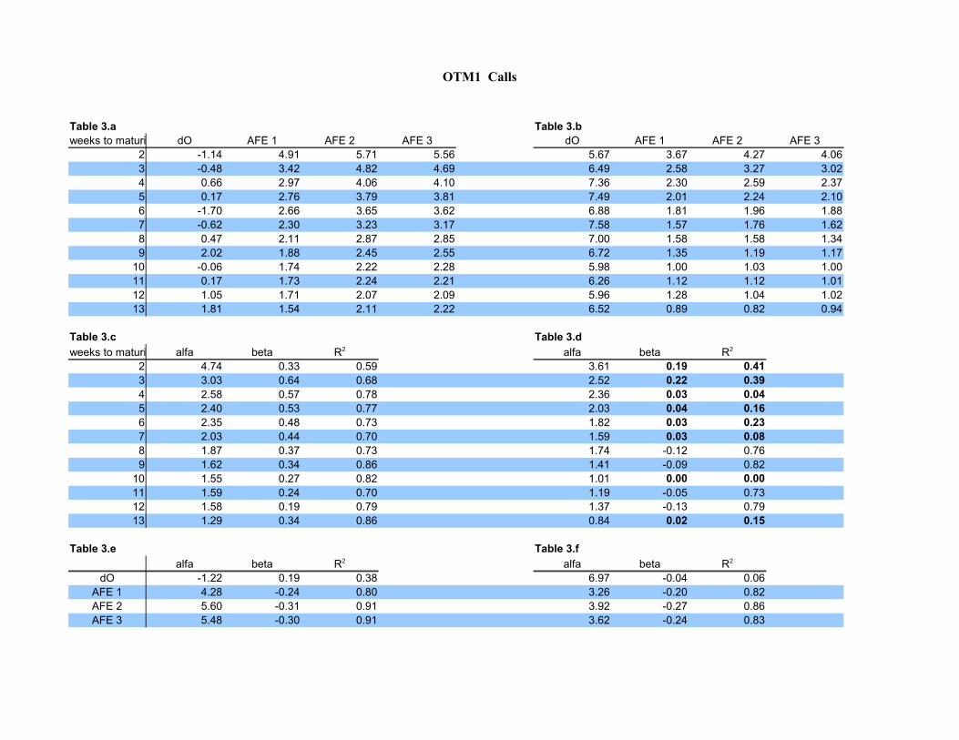
1.c – 8.c show results from the regressions. I found that only 4 of 96 regressions did not show

a positive relation. Tables 1.d – 8.d summarise the regression result of the second statement.

Here, 36 of 96 regressions did not show negative relation. The regressions revealed that the

mean of AFEs increases as orders of derivatives in use increase. As the expected or desirable

result is the other way around, the mean should go towards zero. The Taylor approximation is

less exact when more derivatives are considered, the option price changes does not follow a T-

E of BS. The standard deviation on the other hand is often decreasing when higher order

derivatives are considered. This is true for about 2/3 of the data. Interpretation of decreasing

standard deviation is that BS always predicts price changes with about the same error.

II. The mean of AFEs decreases as time-to-maturity increases. Standard deviation of AFEs

also decreases as time-to-maturity increases.

Tables 1.e – 8.e show regression results from relation between mean of AFEs and time to

maturity. Tables 1.f-8.f shows regression result from relation between standard deviation of

AFEs and time to maturity. All regressions show downward trend for increasing maturity

except for ITM puts. Regressions are also made for observing the relation between δO and

maturity. The regressions show no relation between observed option price and maturity. This

result suggests that while the observed option price changes are rather random and it's

standard deviation is rather constant, the models prediction is more precise as the maturity

increases.

III. Mean of AFEs decreases as moneyness goes from ITM to OTM2. Standard deviation of

22

AFEs also decreases as moneyness goes from ITM to OTM2.

Tables 9.c – 14.c summarise the regression results of the first statement. Only 3 out of 72

regression failed to show positive relation. Tables 9.d – 14.d show how standard deviation

vary with moneyness. Out of 72 regressions, 28 did not show a negative relation. Same

regression was made for observed option price changes for comparison. I found that the mean

of δO increases as moneyness increases/decreases for call/put. As for standard deviation, the

regression betas decreases drastically as strikes go from ITM to OTM2*. For the observed

price changes, the difference between the standard deviation estimated from the ITM options

and from the OTM2 options is large. But once the higher order derivatives are considered, the

difference gets smaller. If standard deviation is considered as risk, the BS derivatives can

eliminate some risk for high risk options, i.e. ITMs and ATMs. Where as for options with less

risk, hedging with BS derivatives will not have much effect.

IV. The difference of AFE from second and third derivatives is only marginal.

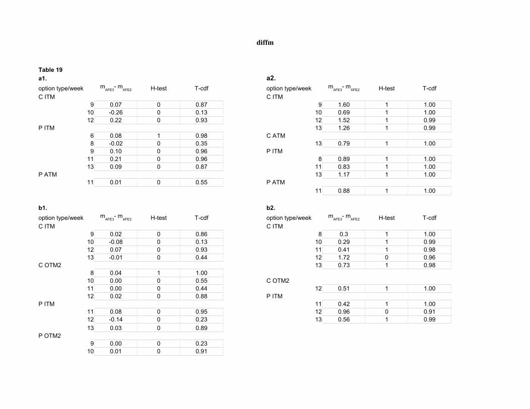
To test the difference between the means of two samples, I will do a two side hypothesis

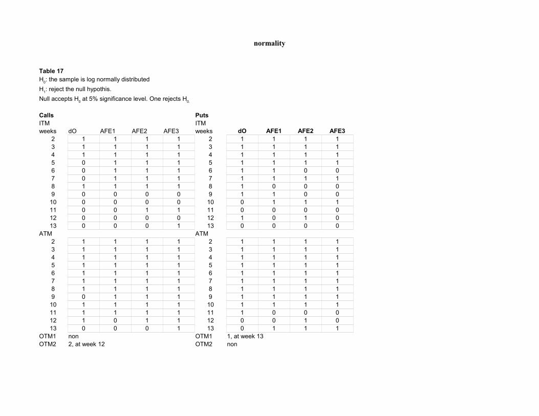
test[18]. This test takes the assumption that the samples are normally distributed. First I have to

perform a normality test on all samples. I use Lilliefors test[19] to test for normality because it

is a non-parametric tes and the mean and standard deviation of the samples does not have to

be known. The mean and standard deviation estimated from the samples are not to be mixed

up with the “real” mean and standard deviation, that is the reason why it is best to use a non-

parametric test. Result from Lilliefors test for all samples are shown in table 17. Most of the

samples are not normally distributed. Normality appears mostly in ITM samples for both calls

and puts, and almost non-existent in OTM-samples. By looking at distributions from

randomly picked samples, I observed that the distributions are often skewed to the left and

leaves a long tail to the right. Since we are analysing absolute errors, all values are greater

than zero. One possible distribution for left side skewness and positive numbers is log normal

* The betas estimated from δO has a range from –1.47 to –5.41, compared to betas estimated from AFEs, which are almost never less than –1

23

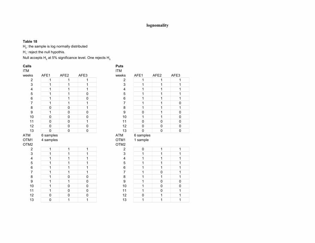
distribution. If AFEs are log normally distributed, then the logarithm of AFEs are normally

distributed. The samples are tested for log normality and the result is shown in table 18. I

found that log normality appear mostly in ITMs and OTM2s and often in maturities longer

than 5 weeks. The mean comparisons will only be made for samples that are nomal or log

normal. The result is shown in 19a. Also I made mean comparisons between AFE1 and AFE2.

The result is shown in 19b. As we can see, statistically speaking, we cannot show that there is

difference between means of AFE2 and AFE3. Whereas we can find significant difference

between means of AFE1 and AFE2. This also supports that option prices do not follow T-E of

BS.

Conclusion

I have come to the following conclusions:

1. Higher order derivatives of BS failed to explain option price changes after 5 holding days.

The mean of AFEs does not decrease as more derivatives are used, which is the result we

expected. This is a parallel to delta vs. gamma hedging. In theory the hedging performance

should be improved by making both delta and gamma neutral, but in practise it is quite the

opposite. Also we cannot find statistic significance in the difference between the means of

AFE2 and AFE3. Should options price follow T-E of BS the mean of AFE 3 should be smaller

than AFE2.

2. Is there additional information in 2:nd and 3:rd order derivatives? Yes, considering the

standard deviation of AFEs are substantially smaller once higher order derivatives are

considered. BS fails to predict the price changes, on the other hand we can predict the

prediction error within a small interval.

3. BS is much better at predicting the longer maturity samples than the short maturity

samples. One explaination could be that the differential equation of BS can describe the

movement of long maturity options quite well, while short maturity options are more sensitive

to new information arrived in the market and cannot be described by the differential equation.

24

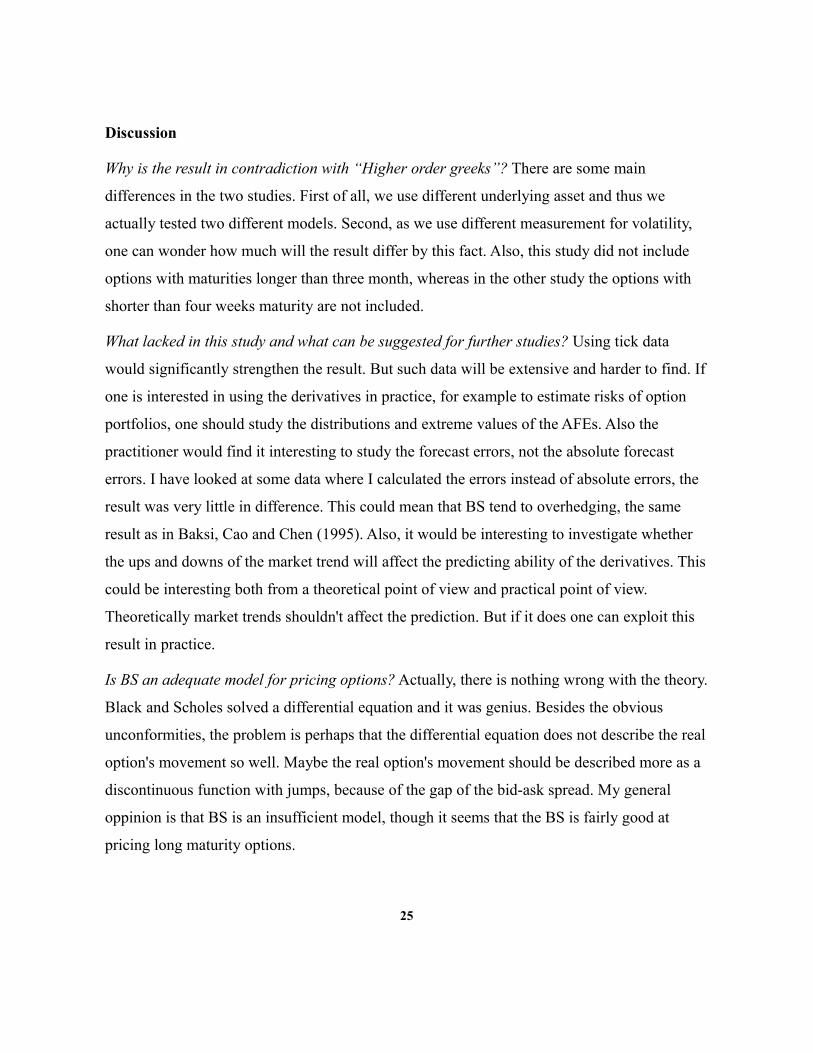
Discussion

Why is the result in contradiction with “Higher order greeks”? There are some main

differences in the two studies. First of all, we use different underlying asset and thus we

actually tested two different models. Second, as we use different measurement for volatility,

one can wonder how much will the result differ by this fact. Also, this study did not include

options with maturities longer than three month, whereas in the other study the options with

shorter than four weeks maturity are not included.

What lacked in this study and what can be suggested for further studies? Using tick data

would significantly strengthen the result. But such data will be extensive and harder to find. If

one is interested in using the derivatives in practice, for example to estimate risks of option

portfolios, one should study the distributions and extreme values of the AFEs. Also the

practitioner would find it interesting to study the forecast errors, not the absolute forecast

errors. I have looked at some data where I calculated the errors instead of absolute errors, the

result was very little in difference. This could mean that BS tend to overhedging, the same

result as in Baksi, Cao and Chen (1995). Also, it would be interesting to investigate whether

the ups and downs of the market trend will affect the predicting ability of the derivatives. This

could be interesting both from a theoretical point of view and practical point of view.

Theoretically market trends shouldn't affect the prediction. But if it does one can exploit this

result in practice.

Is BS an adequate model for pricing options? Actually, there is nothing wrong with the theory.

Black and Scholes solved a differential equation and it was genius. Besides the obvious

unconformities, the problem is perhaps that the differential equation does not describe the real

option's movement so well. Maybe the real option's movement should be described more as a

discontinuous function with jumps, because of the gap of the bid-ask spread. My general

oppinion is that BS is an insufficient model, though it seems that the BS is fairly good at

pricing long maturity options.

25

Endnotes[1] Garber, P.M., Famous first bubbles,1990[2] http://nobelprize.org/nobel_prizes/economics/laureates/1997/press.html[3] http://en.wikipedia.org/wiki/Louis_Bachelier [4] http://hilltop.bradley.edu/~arr/bsm/pg03.html[5] http://nobelprize.org/nobel_prizes/economics/laureates/1997/press.html[6] Haug, E.G. and N.N. Taleb, Why we have never used the Black-Scholes-Merton Option

Pricing Formula, 2008[7] Black, F. and M. Scholes, The pricing of options and corporate liabilities, 1973[8] Hull, J.C. Options, futures and other derivatives. 2006 p.335[9] Hull, J.C. Options, futures and other derivatives. 2006 p.334[10] Ederington, L. and W. Guan, Why are these options smiling, 2002[11] Foresi, S. and L. Wu, Crashophobia: a domestic fear or world wild concern?, 2005[12] http://www.nasdaqomxnordic.com/indexes/historical_prices/ ?

Instrument=SSESE0000337842 [13] http://www.riksbank.se/templates/Page.aspx?id=15963 [14] Black, F. and M. Scholes, The pricing of options and corporate liabilities, 1973[15] Ederington, L. and W. Guan, Higher Order Greeks, 2007[16] Forsling, G. and M. Neymark, Matematisk analys en variabel, 2004 p.353[17] Blom, G. and B. Holmquist, Statistikteori med tillämpningar, 1998 p.149[18] Blom, G. and B. Holmquist, Statistikteori med tillämpningar, 1998 p.102[19] Matlab Help, lillietest.

26

http://nobelprize.org/nobel_prizes/economics/laureates/1997/press.html

http://www.riksbank.se/templates/Page.aspx?id=15963

http://www.nasdaqomxnordic.com/indexes/historical_prices/?Instrument=SSESE0000337842



http://www.nasdaqomxnordic.com/indexes/historical_prices/



http://hilltop.bradley.edu/~arr/bsm/pg03.html


http://en.wikipedia.org/wiki/Louis_Bachelier



References

Books

Forsling, G. and M. Neymark, Matematisk analys en variabel, 2004Blom, G. and B. Holmquist, Statistikteori med tillämpningar, 1998Nelson, S.A., The A B C of Options and Arbitrage, 1904

Articles

Baksi, G., C. Cao and Z. Chen, Empirical performance of alternative option pricing model, 1995Black, F. and M. Scholes, The valuation of option contracts and a test of market efficiency, 1972Black, F. and M. Scholes, The pricing of options and corporate liabilities, 1973Chiras, D. and S. Manaster, The information content of option prices and a test of market efficiency, 1978Ederington, L. and W. Guan, Why are these options smiling, 2002Ederington, L. and W. Guan, Higher Order Greeks, 2007Foresi, S. and L. Wu, Crashophobia: a domestic fear or world wild concern?, 2005Galai, D., Tests of market efficiency and the Chicago Board Options Exchange, 1977Garber, P.M., Famous first bubbles,1990Haug, E.G. and N.N. Taleb, Why we have never used the Black-Scholes-Merton option pricing formula, 2008

Internet

http://nobelprize.org/nobel_prizes/economics/laureates/1997/press.htmlhttp://en.wikipedia.org/wiki/Louis_Bachelier http://hilltop.bradley.edu/~arr/bsm/pg03.html http://www.nasdaqomxnordic.com/indexes/historical_prices/?Instrument=SSESE0000337842http://www.riksbank.se/templates/Page.aspx?id=15963

27

http://www.riksbank.se/templates/Page.aspx?id=15963


http://hilltop.bradley.edu/~arr/bsm/pg03.html

http://en.wikipedia.org/wiki/Louis_Bachelier


Appendix:

Tables

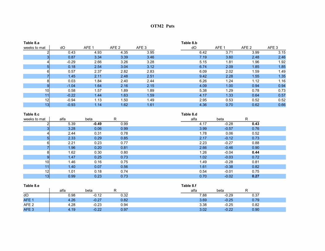
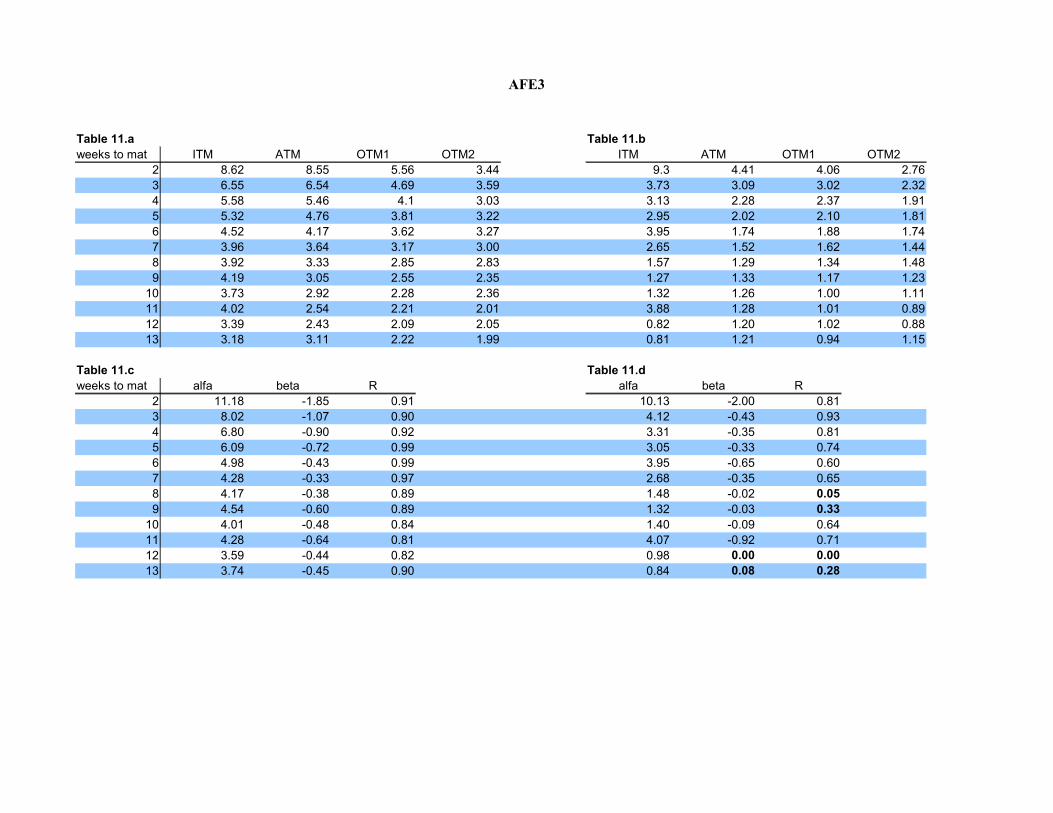
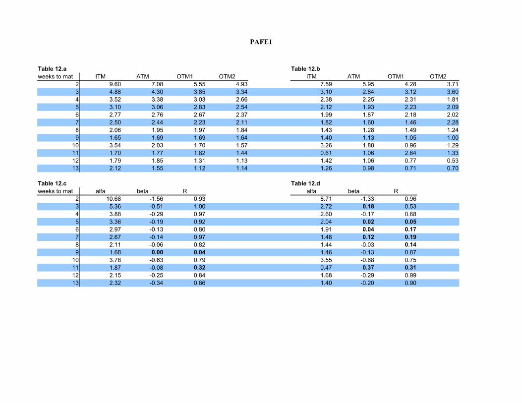
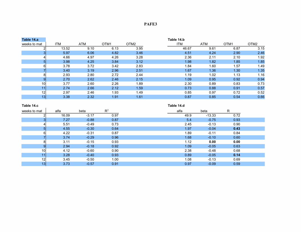
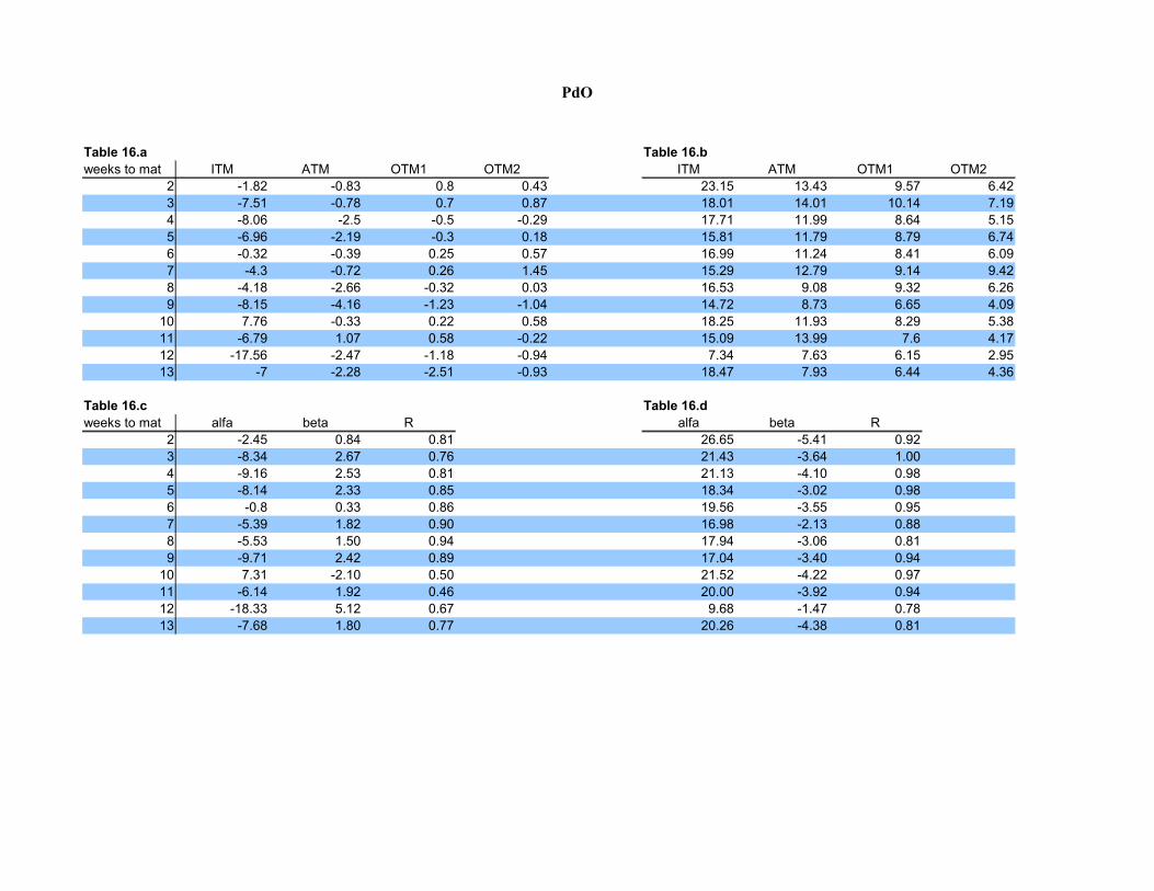
Tables 1-4 show the result of the four call strike samples. Table 5-8 show the result of the four put strike samples. Tables 9-16 show the same result as tables 1-8 but are organised after AFE (absolute forecast error). For the tables 1-16, the a-tables show the means of the samples, whereas b-tables show the standard deviations. C-tables display the regression results from testing the relation between mean and AFE. Alfa is where the linear function intersect with the y-axe. Beta is the slope of the line and R2 is how much of the data can be explained by the function. D-tables are regression result from testing the relation between standard deviation and AFE. E-tables are the results from testing the relation between mean and maturity. F-tables are the results from testing the relation between standard deviation and maturity. The numbers that are bold mark the regressions that violate against the assumed relations. Table 17 displays the test result from testing normality. Table 18 shows test result from testing log normality. Table 19.a1 and b1 show the test result from testing whether there or not there is difference between the mean of AFE2 and AFE3. Table 19.a2 and b2 show the test result from testing the difference between the mean of AFE1 and AFE2. Table 19.a test the samples that showed normality, based on result from table 17. Table 19.b test the sample that showed log normality, based on result from table 18.

ITM Calls

Table 1.a Table 1.bweeks to maturity dO AFE 1 AFE 2 AFE 3 dO AFE 1 AFE 2 AFE 3

2 -9.09 7.73 8.61 8.62 16.44 5.66 5.55 9.33 -8.95 5.51 6.00 6.55 16.80 4.59 2.93 3.734 -4.94 4.32 5.64 5.58 17.49 3.27 5.06 3.135 -7.17 4.37 5.03 5.32 15.14 4.54 2.19 2.956 -6.61 3.76 4.51 4.52 12.31 3.20 2.75 3.957 -6.43 3.52 3.93 3.96 14.14 5.14 2.74 2.658 -8.91 3.45 3.74 3.92 18.03 3.41 1.33 1.579 -8.33 2.52 4.12 4.19 14.76 1.76 1.22 1.27

10 -7.78 3.30 3.99 3.73 12.93 1.53 1.26 1.3211 -4.06 2.89 3.78 4.02 13.28 2.19 1.43 3.8812 -3.54 1.65 3.17 3.39 12.99 1.86 0.84 0.8213 -5.89 1.92 3.17 3.18 10.93 1.18 0.61 0.81

Table 1.c Table 1.dweeks to maturity alfa beta alfa beta

2 7.43 0.44 0.76 3.19 1.82 0.733 4.98 0.52 1.00 4.61 -0.43 0.274 3.93 0.63 0.71 3.96 -0.07 0.005 3.96 0.47 0.95 4.82 -0.80 0.446 3.50 0.38 0.77 2.56 0.37 0.387 3.36 0.22 0.81 6.00 -1.24 0.788 3.23 0.24 0.98 3.94 -0.92 0.659 1.94 0.84 0.78 1.90 -0.24 0.67

10 3.24 0.21 0.38 1.58 -0.10 0.5411 2.43 0.57 0.90 0.81 0.84 0.4512 1.00 0.87 0.84 2.22 -0.52 0.7613 1.49 0.63 0.75 1.24 -0.19 0.41

Table 1.e Table 1.falfa beta alfa beta

dO -8.89 0.28 0.27 17.86 -0.43 0.49AFE 1 6.84 -0.41 0.81 5.88 -0.36 0.73AFE 2 7.39 -0.37 0.74 5.19 -0.38 0.75AFE 3 7.58 -0.38 0.76 6.4 -0.46 0.51

R2 R2

R2 R2

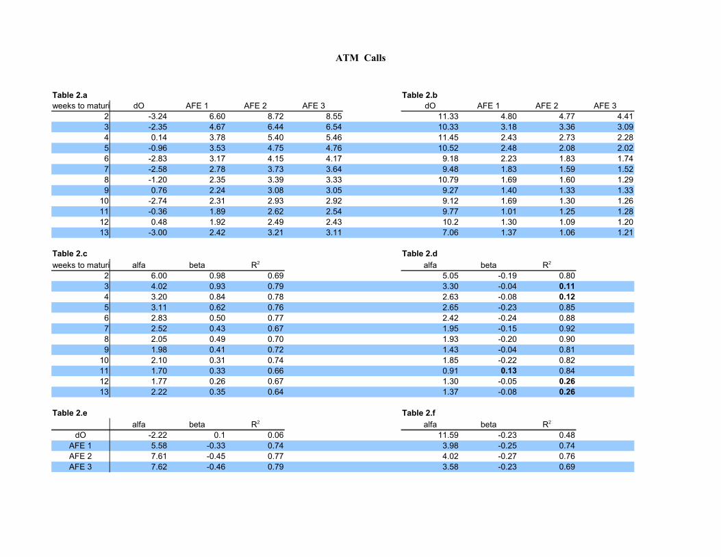
ATM Calls


2 -3.24 6.60 8.72 8.55 11.33 4.80 4.77 4.413 -2.35 4.67 6.44 6.54 10.33 3.18 3.36 3.094 0.14 3.78 5.40 5.46 11.45 2.43 2.73 2.285 -0.96 3.53 4.75 4.76 10.52 2.48 2.08 2.026 -2.83 3.17 4.15 4.17 9.18 2.23 1.83 1.747 -2.58 2.78 3.73 3.64 9.48 1.83 1.59 1.528 -1.20 2.35 3.39 3.33 10.79 1.69 1.60 1.299 0.76 2.24 3.08 3.05 9.27 1.40 1.33 1.33

10 -2.74 2.31 2.93 2.92 9.12 1.69 1.30 1.2611 -0.36 1.89 2.62 2.54 9.77 1.01 1.25 1.2812 0.48 1.92 2.49 2.43 10.2 1.30 1.09 1.2013 -3.00 2.42 3.21 3.11 7.06 1.37 1.06 1.21


2 6.00 0.98 0.69 5.05 -0.19 0.803 4.02 0.93 0.79 3.30 -0.04 0.114 3.20 0.84 0.78 2.63 -0.08 0.125 3.11 0.62 0.76 2.65 -0.23 0.856 2.83 0.50 0.77 2.42 -0.24 0.887 2.52 0.43 0.67 1.95 -0.15 0.928 2.05 0.49 0.70 1.93 -0.20 0.909 1.98 0.41 0.72 1.43 -0.04 0.81

10 2.10 0.31 0.74 1.85 -0.22 0.8211 1.70 0.33 0.66 0.91 0.13 0.8412 1.77 0.26 0.67 1.30 -0.05 0.2613 2.22 0.35 0.64 1.37 -0.08 0.26


dO -2.22 0.1 0.06 11.59 -0.23 0.48AFE 1 5.58 -0.33 0.74 3.98 -0.25 0.74AFE 2 7.61 -0.45 0.77 4.02 -0.27 0.76AFE 3 7.62 -0.46 0.79 3.58 -0.23 0.69

R2 R2

R2 R2

OTM1 Calls


2 -1.14 4.91 5.71 5.56 5.67 3.67 4.27 4.063 -0.48 3.42 4.82 4.69 6.49 2.58 3.27 3.024 0.66 2.97 4.06 4.10 7.36 2.30 2.59 2.375 0.17 2.76 3.79 3.81 7.49 2.01 2.24 2.106 -1.70 2.66 3.65 3.62 6.88 1.81 1.96 1.887 -0.62 2.30 3.23 3.17 7.58 1.57 1.76 1.628 0.47 2.11 2.87 2.85 7.00 1.58 1.58 1.349 2.02 1.88 2.45 2.55 6.72 1.35 1.19 1.17

10 -0.06 1.74 2.22 2.28 5.98 1.00 1.03 1.0011 0.17 1.73 2.24 2.21 6.26 1.12 1.12 1.0112 1.05 1.71 2.07 2.09 5.96 1.28 1.04 1.0213 1.81 1.54 2.11 2.22 6.52 0.89 0.82 0.94


2 4.74 0.33 0.59 3.61 0.19 0.413 3.03 0.64 0.68 2.52 0.22 0.394 2.58 0.57 0.78 2.36 0.03 0.045 2.40 0.53 0.77 2.03 0.04 0.166 2.35 0.48 0.73 1.82 0.03 0.237 2.03 0.44 0.70 1.59 0.03 0.088 1.87 0.37 0.73 1.74 -0.12 0.769 1.62 0.34 0.86 1.41 -0.09 0.82

10 1.55 0.27 0.82 1.01 0.00 0.0011 1.59 0.24 0.70 1.19 -0.05 0.7312 1.58 0.19 0.79 1.37 -0.13 0.7913 1.29 0.34 0.86 0.84 0.02 0.15


dO -1.22 0.19 0.38 6.97 -0.04 0.06AFE 1 4.28 -0.24 0.80 3.26 -0.20 0.82AFE 2 5.60 -0.31 0.91 3.92 -0.27 0.86AFE 3 5.48 -0.30 0.91 3.62 -0.24 0.83

R2 R2

R2 R2

OTM2 Calls


2 -0.68 4.08 3.65 3.44 3.21 2.78 2.79 2.763 0.36 3.36 3.58 3.59 5.27 2.47 2.32 2.324 0.62 2.47 2.99 3.03 4.96 1.91 1.95 1.915 -0.25 2.35 3.14 3.22 4.93 1.64 1.82 1.816 -1.40 2.39 3.34 3.27 5.07 1.63 1.80 1.747 0.93 2.29 2.99 3.00 7.21 1.52 1.53 1.448 0.57 2.09 2.77 2.83 5.57 1.42 1.52 1.489 1.74 1.66 2.23 2.35 4.74 1.30 1.25 1.23

10 1.12 1.66 2.41 2.36 7.48 1.21 1.26 1.1111 0.62 1.57 2.02 2.01 4.38 1.08 0.87 0.8912 2.25 1.33 1.99 2.05 7.40 0.71 0.80 0.8813 3.51 1.26 1.81 1.99 5.17 0.84 1.06 1.15


2 4.37 -0.32 0.97 2.8 -0.01 0.663 3.28 0.11 0.78 2.52 -0.07 0.784 2.26 0.28 0.81 1.92 0.00 0.035 2.04 0.43 0.82 1.59 0.08 0.736 2.13 0.44 0.69 1.61 0.06 0.427 2.04 0.36 0.77 1.58 -0.04 0.698 1.82 0.37 0.81 1.41 0.03 0.359 1.39 0.34 0.88 1.33 -0.04 0.97

10 1.44 0.35 0.70 1.30 -0.05 0.4111 1.42 0.22 0.75 1.14 -0.1 0.6912 1.08 0.36 0.81 0.63 0.08 1.0013 0.97 0.36 0.92 0.70 0.16 0.95


dO -1.29 0.28 0.58 4.22 0.16 0.21AFE 1 3.82 -0.21 0.86 2.75 -0.16 0.90AFE 2 4.01 -0.17 0.92 2.75 -0.16 0.91AFE 3 3.92 -0.15 0.91 2.68 -0.15 0.88

R2 R2

R2 R2

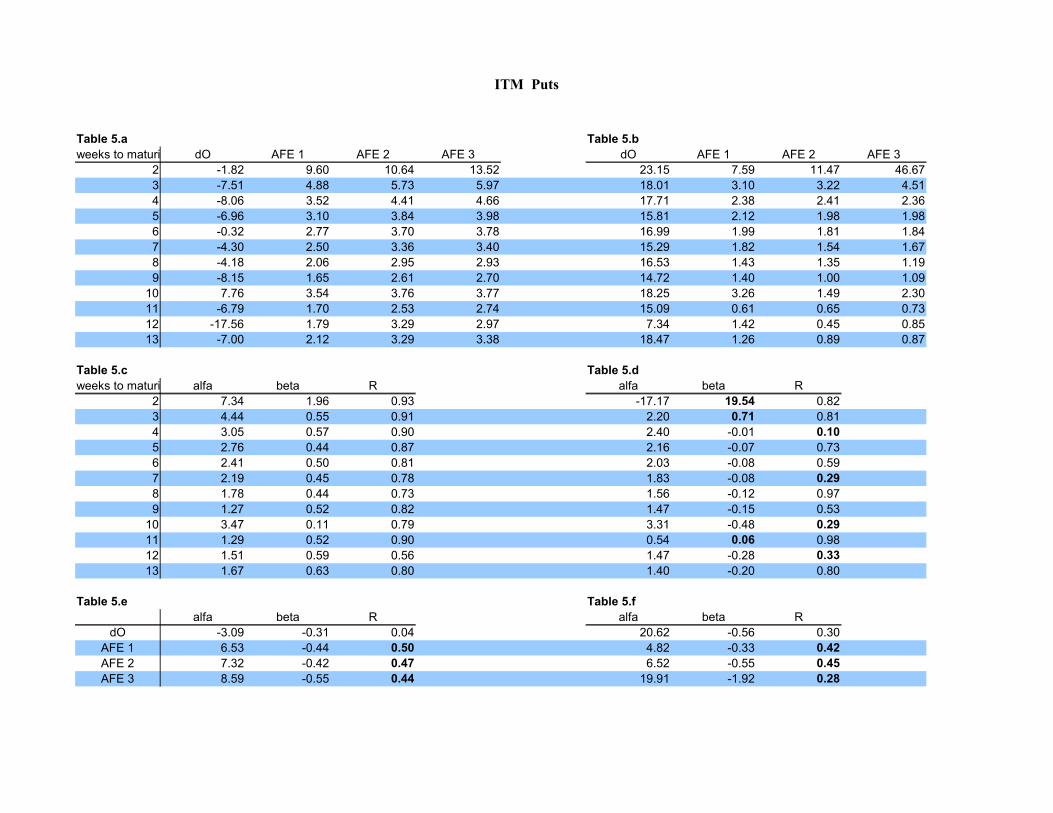
ITM Puts


2 -1.82 9.60 10.64 13.52 23.15 7.59 11.47 46.673 -7.51 4.88 5.73 5.97 18.01 3.10 3.22 4.514 -8.06 3.52 4.41 4.66 17.71 2.38 2.41 2.365 -6.96 3.10 3.84 3.98 15.81 2.12 1.98 1.986 -0.32 2.77 3.70 3.78 16.99 1.99 1.81 1.847 -4.30 2.50 3.36 3.40 15.29 1.82 1.54 1.678 -4.18 2.06 2.95 2.93 16.53 1.43 1.35 1.199 -8.15 1.65 2.61 2.70 14.72 1.40 1.00 1.09

10 7.76 3.54 3.76 3.77 18.25 3.26 1.49 2.3011 -6.79 1.70 2.53 2.74 15.09 0.61 0.65 0.7312 -17.56 1.79 3.29 2.97 7.34 1.42 0.45 0.8513 -7.00 2.12 3.29 3.38 18.47 1.26 0.89 0.87

Table 5.c Table 5.dweeks to maturity alfa beta R alfa beta R

2 7.34 1.96 0.93 -17.17 19.54 0.823 4.44 0.55 0.91 2.20 0.71 0.814 3.05 0.57 0.90 2.40 -0.01 0.105 2.76 0.44 0.87 2.16 -0.07 0.736 2.41 0.50 0.81 2.03 -0.08 0.597 2.19 0.45 0.78 1.83 -0.08 0.298 1.78 0.44 0.73 1.56 -0.12 0.979 1.27 0.52 0.82 1.47 -0.15 0.53

10 3.47 0.11 0.79 3.31 -0.48 0.2911 1.29 0.52 0.90 0.54 0.06 0.9812 1.51 0.59 0.56 1.47 -0.28 0.3313 1.67 0.63 0.80 1.40 -0.20 0.80

Table 5.e Table 5.falfa beta R alfa beta R

dO -3.09 -0.31 0.04 20.62 -0.56 0.30AFE 1 6.53 -0.44 0.50 4.82 -0.33 0.42AFE 2 7.32 -0.42 0.47 6.52 -0.55 0.45AFE 3 8.59 -0.55 0.44 19.91 -1.92 0.28

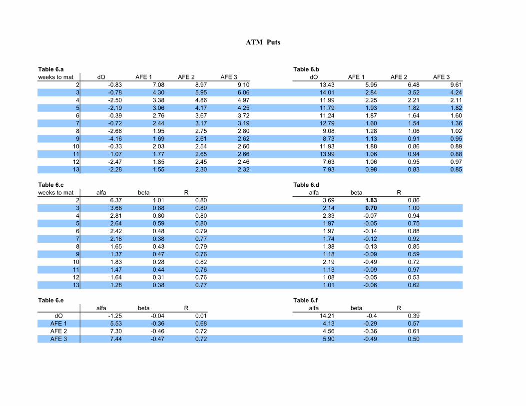
ATM Puts

Table 6.a Table 6.bweeks to mat dO AFE 1 AFE 2 AFE 3 dO AFE 1 AFE 2 AFE 3

2 -0.83 7.08 8.97 9.10 13.43 5.95 6.48 9.613 -0.78 4.30 5.95 6.06 14.01 2.84 3.52 4.244 -2.50 3.38 4.86 4.97 11.99 2.25 2.21 2.115 -2.19 3.06 4.17 4.25 11.79 1.93 1.82 1.826 -0.39 2.76 3.67 3.72 11.24 1.87 1.64 1.607 -0.72 2.44 3.17 3.19 12.79 1.60 1.54 1.368 -2.66 1.95 2.75 2.80 9.08 1.28 1.06 1.029 -4.16 1.69 2.61 2.62 8.73 1.13 0.91 0.95

10 -0.33 2.03 2.54 2.60 11.93 1.88 0.86 0.8911 1.07 1.77 2.65 2.66 13.99 1.06 0.94 0.8812 -2.47 1.85 2.45 2.46 7.63 1.06 0.95 0.9713 -2.28 1.55 2.30 2.32 7.93 0.98 0.83 0.85

Table 6.c Table 6.dweeks to mat alfa beta R alfa beta R

2 6.37 1.01 0.80 3.69 1.83 0.863 3.68 0.88 0.80 2.14 0.70 1.004 2.81 0.80 0.80 2.33 -0.07 0.945 2.64 0.59 0.80 1.97 -0.05 0.756 2.42 0.48 0.79 1.97 -0.14 0.887 2.18 0.38 0.77 1.74 -0.12 0.928 1.65 0.43 0.79 1.38 -0.13 0.859 1.37 0.47 0.76 1.18 -0.09 0.59

10 1.83 0.28 0.82 2.19 -0.49 0.7211 1.47 0.44 0.76 1.13 -0.09 0.9712 1.64 0.31 0.76 1.08 -0.05 0.5313 1.28 0.38 0.77 1.01 -0.06 0.62


dO -1.25 -0.04 0.01 14.21 -0.4 0.39AFE 1 5.53 -0.36 0.68 4.13 -0.29 0.57AFE 2 7.30 -0.46 0.72 4.56 -0.36 0.61AFE 3 7.44 -0.47 0.72 5.90 -0.49 0.50

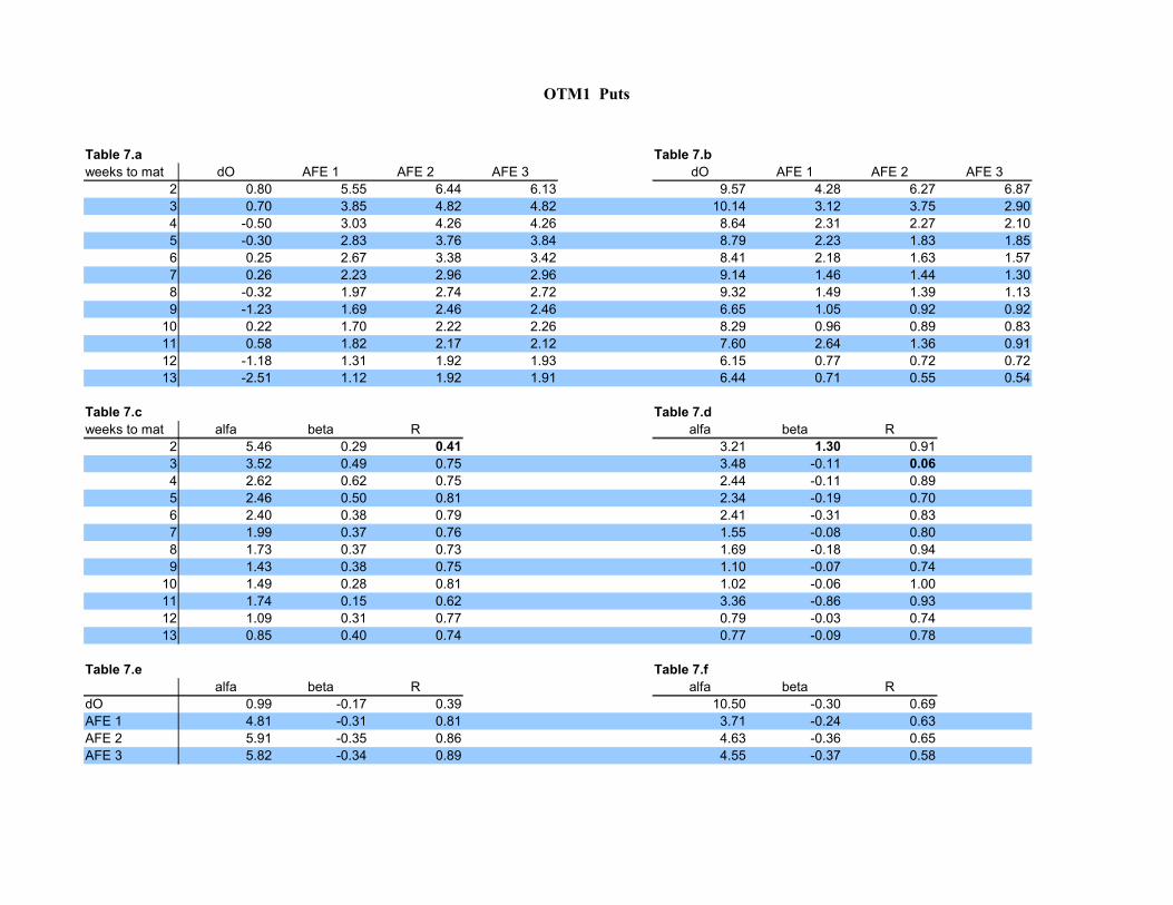
OTM1 Puts


2 0.80 5.55 6.44 6.13 9.57 4.28 6.27 6.873 0.70 3.85 4.82 4.82 10.14 3.12 3.75 2.904 -0.50 3.03 4.26 4.26 8.64 2.31 2.27 2.105 -0.30 2.83 3.76 3.84 8.79 2.23 1.83 1.856 0.25 2.67 3.38 3.42 8.41 2.18 1.63 1.577 0.26 2.23 2.96 2.96 9.14 1.46 1.44 1.308 -0.32 1.97 2.74 2.72 9.32 1.49 1.39 1.139 -1.23 1.69 2.46 2.46 6.65 1.05 0.92 0.92

10 0.22 1.70 2.22 2.26 8.29 0.96 0.89 0.8311 0.58 1.82 2.17 2.12 7.60 2.64 1.36 0.9112 -1.18 1.31 1.92 1.93 6.15 0.77 0.72 0.7213 -2.51 1.12 1.92 1.91 6.44 0.71 0.55 0.54


2 5.46 0.29 0.41 3.21 1.30 0.913 3.52 0.49 0.75 3.48 -0.11 0.064 2.62 0.62 0.75 2.44 -0.11 0.895 2.46 0.50 0.81 2.34 -0.19 0.706 2.40 0.38 0.79 2.41 -0.31 0.837 1.99 0.37 0.76 1.55 -0.08 0.808 1.73 0.37 0.73 1.69 -0.18 0.949 1.43 0.38 0.75 1.10 -0.07 0.74

10 1.49 0.28 0.81 1.02 -0.06 1.0011 1.74 0.15 0.62 3.36 -0.86 0.9312 1.09 0.31 0.77 0.79 -0.03 0.7413 0.85 0.40 0.74 0.77 -0.09 0.78


dO 0.99 -0.17 0.39 10.50 -0.30 0.69AFE 1 4.81 -0.31 0.81 3.71 -0.24 0.63AFE 2 5.91 -0.35 0.86 4.63 -0.36 0.65AFE 3 5.82 -0.34 0.89 4.55 -0.37 0.58

OTM2 Puts


2 0.43 4.93 4.35 3.95 6.42 3.71 3.99 3.153 0.87 3.34 3.39 3.46 7.19 3.60 2.48 2.464 -0.29 2.66 3.26 3.28 5.15 1.81 1.96 1.925 0.18 2.54 3.04 3.12 6.74 2.09 1.85 1.856 0.57 2.37 2.82 2.83 6.09 2.02 1.59 1.497 1.45 2.11 2.48 2.51 9.42 2.28 1.55 1.358 0.03 1.84 2.40 2.44 6.26 1.24 1.12 1.169 -1.04 1.64 2.16 2.15 4.09 1.00 0.94 0.94

10 0.58 1.57 1.89 1.89 5.38 1.29 0.78 0.7311 -0.22 1.44 1.63 1.59 4.17 1.33 0.64 0.5712 -0.94 1.13 1.50 1.49 2.95 0.53 0.52 0.5213 -0.93 1.14 1.62 1.61 4.36 0.70 0.62 0.66


2 5.39 -0.49 0.99 4.17 -0.28 0.433 3.28 0.06 0.99 3.99 -0.57 0.764 2.44 0.31 0.78 1.78 0.06 0.525 2.33 0.29 0.85 2.17 -0.12 0.736 2.21 0.23 0.77 2.23 -0.27 0.887 1.96 0.20 0.81 2.66 -0.46 0.908 1.62 0.30 0.80 1.26 -0.04 0.449 1.47 0.25 0.73 1.02 -0.03 0.72

10 1.46 0.16 0.75 1.49 -0.28 0.8111 1.40 0.07 0.56 1.61 -0.38 0.8212 1.01 0.18 0.74 0.54 -0.01 0.7513 0.99 0.23 0.73 0.70 -0.02 0.27


dO 0.98 -0.12 0.32 7.88 -0.29 0.37AFE 1 4.26 -0.27 0.82 3.69 -0.25 0.79AFE 2 4.28 -0.23 0.94 3.38 -0.25 0.82AFE 3 4.19 -0.22 0.97 3.02 -0.22 0.90

AFE1

Table 9.a Table 9.bweeks to mat ITM ATM OTM1 OTM2 ITM ATM OTM1 OTM2

2 7.73 6.60 4.91 4.08 5.66 4.80 3.67 2.783 5.51 4.67 3.42 3.36 4.59 3.18 2.58 2.474 4.32 3.78 2.97 2.47 3.27 2.43 2.30 1.915 4.37 3.53 2.76 2.35 4.54 2.48 2.01 1.646 3.76 3.17 2.66 2.39 3.20 2.23 1.81 1.637 3.52 2.78 2.30 2.29 5.14 1.83 1.57 1.528 3.45 2.35 2.11 2.09 3.41 1.69 1.58 1.429 2.52 2.24 1.88 1.66 1.76 1.40 1.35 1.30

10 3.30 2.31 1.74 1.66 1.53 1.69 1.00 1.2111 2.89 1.89 1.73 1.57 2.19 1.01 1.12 1.0812 1.65 1.92 1.71 1.33 1.86 1.30 1.28 0.7113 1.92 2.42 1.54 1.26 1.18 1.37 0.89 0.84


2 8.99 -1.26 0.98 6.67 -0.97 1.003 6.16 -0.77 0.91 4.95 -0.70 0.854 4.98 -0.64 0.99 3.53 -0.42 0.905 4.95 -0.68 0.98 4.96 -0.91 0.846 4.15 -0.46 0.97 3.5 -0.51 0.897 3.77 -0.42 0.87 5.29 -1.11 0.678 3.58 -0.43 0.75 3.54 -0.61 0.719 2.81 -0.29 0.99 1.81 -0.14 0.79

10 3.63 -0.55 0.88 1.77 -0.17 0.4711 3.05 -0.41 0.80 2.16 -0.32 0.5512 1.94 -0.12 0.37 2.16 -0.35 0.9113 2.49 -0.28 0.54 1.45 -0.15 0.60

AFE2


2 8.61 8.72 5.71 3.65 5.55 4.77 4.27 2.793 6.00 6.44 4.82 3.58 2.93 3.36 3.27 2.324 5.64 5.40 4.06 2.99 5.06 2.73 2.59 1.955 5.03 4.75 3.79 3.14 2.19 2.08 2.24 1.826 4.51 4.15 3.65 3.34 2.75 1.83 1.96 1.807 3.93 3.73 3.23 2.99 2.74 1.59 1.76 1.538 3.74 3.39 2.87 2.77 1.33 1.60 1.58 1.529 4.12 3.08 2.45 2.23 1.22 1.33 1.19 1.25

10 3.99 2.93 2.22 2.41 1.26 1.30 1.03 1.2611 3.78 2.62 2.24 2.02 1.43 1.25 1.12 0.8712 3.17 2.49 2.07 1.99 0.84 1.09 1.04 0.8013 3.17 3.21 2.11 1.81 0.61 1.06 0.82 1.06


2 11.14 -1.79 0.89 6.54 -0.88 0.953 7.43 -0.89 0.80 3.44 -0.19 0.274 6.85 -0.93 0.94 5.45 -0.95 0.815 5.84 -0.67 0.96 2.32 -0.10 0.456 4.91 -0.40 0.99 2.76 -0.27 0.617 4.3 -0.33 0.97 2.77 -0.35 0.638 4.05 -0.34 0.95 1.38 0.05 0.319 4.54 -0.63 0.92 1.26 0.00 0.01

10 4.25 -0.55 0.79 1.28 -0.03 0.0711 4.08 -0.57 0.87 1.62 -0.18 0.9812 3.42 -0.40 0.89 0.99 -0.02 0.0213 3.87 -0.52 0.86 0.61 0.11 0.45

AFE3


2 8.62 8.55 5.56 3.44 9.3 4.41 4.06 2.763 6.55 6.54 4.69 3.59 3.73 3.09 3.02 2.324 5.58 5.46 4.1 3.03 3.13 2.28 2.37 1.915 5.32 4.76 3.81 3.22 2.95 2.02 2.10 1.816 4.52 4.17 3.62 3.27 3.95 1.74 1.88 1.747 3.96 3.64 3.17 3.00 2.65 1.52 1.62 1.448 3.92 3.33 2.85 2.83 1.57 1.29 1.34 1.489 4.19 3.05 2.55 2.35 1.27 1.33 1.17 1.23

10 3.73 2.92 2.28 2.36 1.32 1.26 1.00 1.1111 4.02 2.54 2.21 2.01 3.88 1.28 1.01 0.8912 3.39 2.43 2.09 2.05 0.82 1.20 1.02 0.8813 3.18 3.11 2.22 1.99 0.81 1.21 0.94 1.15


2 11.18 -1.85 0.91 10.13 -2.00 0.813 8.02 -1.07 0.90 4.12 -0.43 0.934 6.80 -0.90 0.92 3.31 -0.35 0.815 6.09 -0.72 0.99 3.05 -0.33 0.746 4.98 -0.43 0.99 3.95 -0.65 0.607 4.28 -0.33 0.97 2.68 -0.35 0.658 4.17 -0.38 0.89 1.48 -0.02 0.059 4.54 -0.60 0.89 1.32 -0.03 0.33

10 4.01 -0.48 0.84 1.40 -0.09 0.6411 4.28 -0.64 0.81 4.07 -0.92 0.7112 3.59 -0.44 0.82 0.98 0.00 0.0013 3.74 -0.45 0.90 0.84 0.08 0.28

PAFE1


2 9.60 7.08 5.55 4.93 7.59 5.95 4.28 3.713 4.88 4.30 3.85 3.34 3.10 2.84 3.12 3.604 3.52 3.38 3.03 2.66 2.38 2.25 2.31 1.815 3.10 3.06 2.83 2.54 2.12 1.93 2.23 2.096 2.77 2.76 2.67 2.37 1.99 1.87 2.18 2.027 2.50 2.44 2.23 2.11 1.82 1.60 1.46 2.288 2.06 1.95 1.97 1.84 1.43 1.28 1.49 1.249 1.65 1.69 1.69 1.64 1.40 1.13 1.05 1.00

10 3.54 2.03 1.70 1.57 3.26 1.88 0.96 1.2911 1.70 1.77 1.82 1.44 0.61 1.06 2.64 1.3312 1.79 1.85 1.31 1.13 1.42 1.06 0.77 0.5313 2.12 1.55 1.12 1.14 1.26 0.98 0.71 0.70


2 10.68 -1.56 0.93 8.71 -1.33 0.963 5.36 -0.51 1.00 2.72 0.18 0.534 3.88 -0.29 0.97 2.60 -0.17 0.685 3.36 -0.19 0.92 2.04 0.02 0.056 2.97 -0.13 0.80 1.91 0.04 0.177 2.67 -0.14 0.97 1.48 0.12 0.198 2.11 -0.06 0.82 1.44 -0.03 0.149 1.68 0.00 0.04 1.46 -0.13 0.87

10 3.78 -0.63 0.79 3.55 -0.68 0.7511 1.87 -0.08 0.32 0.47 0.37 0.3112 2.15 -0.25 0.84 1.68 -0.29 0.9913 2.32 -0.34 0.86 1.40 -0.20 0.90

PAFE2


2 10.64 8.97 6.44 4.35 11.47 6.48 6.27 3.993 5.73 5.95 4.82 3.39 3.22 3.52 3.75 2.484 4.41 4.86 4.26 3.26 2.41 2.21 2.27 1.965 3.84 4.17 3.76 3.04 1.98 1.82 1.83 1.856 3.70 3.67 3.38 2.82 1.81 1.64 1.63 1.597 3.36 3.17 2.96 2.48 1.54 1.54 1.44 1.558 2.95 2.75 2.74 2.40 1.35 1.06 1.39 1.129 2.61 2.61 2.46 2.16 1.00 0.91 0.92 0.94

10 3.76 2.54 2.22 1.89 1.49 0.86 0.89 0.7811 2.53 2.65 2.17 1.63 0.65 0.94 1.36 0.6412 3.29 2.45 1.92 1.50 0.45 0.95 0.72 0.5213 3.29 2.30 1.92 1.62 0.89 0.83 0.55 0.62


2 12.94 -2.14 0.99 12.71 -2.26 0.863 7.01 -0.81 0.82 3.74 -0.20 0.214 5.21 -0.41 0.61 2.54 -0.13 0.795 4.4 -0.28 0.58 1.97 -0.04 0.486 4.13 -0.29 0.85 1.84 -0.07 0.817 3.71 -0.29 0.94 1.54 -0.01 0.048 3.12 -0.17 0.88 1.31 -0.03 0.079 2.83 -0.15 0.83 0.98 -0.02 0.28

10 4.08 -0.59 0.88 1.53 -0.21 0.6811 3.04 -0.32 0.80 0.81 0.04 0.0212 3.77 -0.59 0.97 0.66 0.00 0.0013 3.63 -0.54 0.92 1 -0.11 0.74

PAFE3


2 13.52 9.10 6.13 3.95 46.67 9.61 6.87 3.153 5.97 6.06 4.82 3.46 4.51 4.24 2.90 2.464 4.66 4.97 4.26 3.28 2.36 2.11 2.10 1.925 3.98 4.25 3.84 3.12 1.98 1.82 1.85 1.856 3.78 3.72 3.42 2.83 1.84 1.60 1.57 1.497 3.40 3.19 2.96 2.51 1.67 1.36 1.30 1.358 2.93 2.80 2.72 2.44 1.19 1.02 1.13 1.169 2.70 2.62 2.46 2.15 1.09 0.95 0.92 0.94

10 3.77 2.60 2.26 1.89 2.30 0.89 0.83 0.7311 2.74 2.66 2.12 1.59 0.73 0.88 0.91 0.5712 2.97 2.46 1.93 1.49 0.85 0.97 0.72 0.5213 3.38 2.32 1.91 1.61 0.87 0.85 0.54 0.66

Table 14.c Table 14.dweeks to mat alfa beta alfa beta R

2 16.09 -3.17 0.97 49.9 -13.33 0.723 7.27 -0.88 0.87 5.4 -0.75 0.934 5.51 -0.49 0.73 2.45 -0.13 0.905 4.55 -0.30 0.64 1.97 -0.04 0.436 4.22 -0.31 0.87 1.89 -0.11 0.847 3.74 -0.29 0.96 1.68 -0.10 0.608 3.11 -0.15 0.93 1.12 0.00 0.009 2.94 -0.18 0.92 1.09 -0.05 0.63

10 4.12 -0.60 0.90 2.38 -0.48 0.6811 3.28 -0.40 0.93 0.89 -0.05 0.1412 3.45 -0.50 1.00 1.08 -0.13 0.6913 3.73 -0.57 0.91 0.97 -0.09 0.59

R2

dO


2 -9.09 -3.24 -1.14 -0.68 16.44 11.33 5.67 3.213 -8.95 -2.35 -0.48 0.36 16.8 10.33 6.49 5.274 -4.94 0.14 0.66 0.62 17.49 11.45 7.36 4.965 -7.17 -0.96 0.17 -0.25 15.14 10.52 7.49 4.936 -6.61 -2.83 -1.7 -1.4 12.31 9.18 6.88 5.077 -6.43 -2.58 -0.62 0.93 14.14 9.48 7.58 7.218 -8.91 -1.2 0.47 0.57 18.03 10.79 7 5.579 -8.33 0.76 2.02 1.74 14.76 9.27 6.72 4.74

10 -7.78 -2.74 -0.06 1.12 12.93 9.12 5.98 7.4811 -4.06 -0.36 0.17 0.62 13.28 9.77 6.26 4.3812 -3.54 0.48 1.05 2.25 12.99 10.2 5.96 7.413 -5.89 -3 1.81 3.51 10.93 7.06 6.52 5.17


2 -10.37 2.73 0.83 20.5 -4.53 0.983 -10.3 2.98 0.83 19.33 -3.84 0.914 -5.18 1.72 0.67 20.73 -4.17 0.965 -7.52 2.19 0.67 17.93 -3.37 0.986 -7.32 1.67 0.82 14.37 -2.40 0.987 -8.18 2.40 0.95 15.27 -2.27 0.858 -9.8 3.01 0.75 20.64 -4.12 0.919 -8.82 3.15 0.67 17.03 -3.26 0.94

10 -9.71 2.94 0.92 13.75 -1.95 0.7111 -4.55 1.46 0.77 15.97 -3.02 0.9812 -4.43 1.80 0.85 14.38 -2.10 0.7613 -9.14 3.30 0.97 11.87 -1.78 0.87

PdO


2 -1.82 -0.83 0.8 0.43 23.15 13.43 9.57 6.423 -7.51 -0.78 0.7 0.87 18.01 14.01 10.14 7.194 -8.06 -2.5 -0.5 -0.29 17.71 11.99 8.64 5.155 -6.96 -2.19 -0.3 0.18 15.81 11.79 8.79 6.746 -0.32 -0.39 0.25 0.57 16.99 11.24 8.41 6.097 -4.3 -0.72 0.26 1.45 15.29 12.79 9.14 9.428 -4.18 -2.66 -0.32 0.03 16.53 9.08 9.32 6.269 -8.15 -4.16 -1.23 -1.04 14.72 8.73 6.65 4.09

10 7.76 -0.33 0.22 0.58 18.25 11.93 8.29 5.3811 -6.79 1.07 0.58 -0.22 15.09 13.99 7.6 4.1712 -17.56 -2.47 -1.18 -0.94 7.34 7.63 6.15 2.9513 -7 -2.28 -2.51 -0.93 18.47 7.93 6.44 4.36


2 -2.45 0.84 0.81 26.65 -5.41 0.923 -8.34 2.67 0.76 21.43 -3.64 1.004 -9.16 2.53 0.81 21.13 -4.10 0.985 -8.14 2.33 0.85 18.34 -3.02 0.986 -0.8 0.33 0.86 19.56 -3.55 0.957 -5.39 1.82 0.90 16.98 -2.13 0.888 -5.53 1.50 0.94 17.94 -3.06 0.819 -9.71 2.42 0.89 17.04 -3.40 0.94

10 7.31 -2.10 0.50 21.52 -4.22 0.9711 -6.14 1.92 0.46 20.00 -3.92 0.9412 -18.33 5.12 0.67 9.68 -1.47 0.7813 -7.68 1.80 0.77 20.26 -4.38 0.81

normality

Table 17

Calls PutsITM ITMweeks dO AFE1 AFE2 AFE3 weeks dO AFE1 AFE2 AFE3

2 1 1 1 1 2 1 1 1 13 1 1 1 1 3 1 1 1 14 1 1 1 1 4 1 1 1 15 0 1 1 1 5 1 1 1 16 0 1 1 1 6 1 1 0 07 0 1 1 1 7 1 1 1 18 1 1 1 1 8 1 0 0 09 0 0 0 0 9 1 1 0 0

10 0 0 0 0 10 0 1 1 111 0 0 1 1 11 0 0 0 012 0 0 0 0 12 1 0 1 013 0 0 0 1 13 0 0 0 0

ATM ATM2 1 1 1 1 2 1 1 1 13 1 1 1 1 3 1 1 1 14 1 1 1 1 4 1 1 1 15 1 1 1 1 5 1 1 1 16 1 1 1 1 6 1 1 1 17 1 1 1 1 7 1 1 1 18 1 1 1 1 8 1 1 1 19 0 1 1 1 9 1 1 1 1

10 1 1 1 1 10 1 1 1 111 1 1 1 1 11 1 0 0 012 1 0 1 1 12 0 0 1 013 0 0 0 1 13 0 1 1 1

OTM1 non OTM1 1, at week 13OTM2 2, at week 12 OTM2 non

H0: the sample is log normally distributed H1: reject the null hypothis. Null accepts H0 at 5% significance level. One rejects H0.

lognomality

Table 18

Calls PutsITM ITMweeks AFE1 AFE2 AFE3 weeks AFE1 AFE2 AFE3

2 1 1 1 2 1 1 13 1 1 1 3 1 1 14 1 1 1 4 1 1 15 1 1 0 5 1 1 16 1 1 0 6 1 1 17 1 1 1 7 1 1 08 0 0 1 8 1 1 19 1 0 0 9 0 1 0

10 0 0 0 10 1 1 011 0 0 1 11 0 0 012 0 0 0 12 0 0 013 0 0 0 13 0 0 0

ATM 6 samples ATM 6 samplesOTM1 4 samples OTM1 1 sampleOTM2 OTM2

2 1 1 1 2 0 1 13 1 1 1 3 1 1 14 1 1 1 4 1 1 15 1 1 1 5 1 1 16 1 1 1 6 1 1 17 1 1 1 7 1 0 18 1 0 0 8 1 1 19 1 1 0 9 1 0 0

10 1 0 0 10 1 0 011 1 0 0 11 1 0 112 0 0 0 12 0 1 113 0 1 1 13 1 1 1

H0: the sample is log normally distributed H1: reject the null hypothis. Null accepts H0 at 5% significance level. One rejects H0.

diffm

Table 19a1. a2.option type/week H-test T-cdf option type/week H-test T-cdfC ITM C ITM

9 0.07 0 0.87 9 1.60 1 1.0010 -0.26 0 0.13 10 0.69 1 1.0012 0.22 0 0.93 12 1.52 1 0.99

P ITM 13 1.26 1 0.996 0.08 1 0.98 C ATM8 -0.02 0 0.35 13 0.79 1 1.009 0.10 0 0.96 P ITM

11 0.21 0 0.96 8 0.89 1 1.0013 0.09 0 0.87 11 0.83 1 1.00

P ATM 13 1.17 1 1.0011 0.01 0 0.55 P ATM

11 0.88 1 1.00

b1. b2.option type/week H-test T-cdf option type/week H-test T-cdfC ITM C ITM

9 0.02 0 0.86 8 0.3 1 1.0010 -0.08 0 0.13 10 0.29 1 0.9912 0.07 0 0.93 11 0.41 1 0.9813 -0.01 0 0.44 12 1.72 0 0.96

C OTM2 13 0.73 1 0.988 0.04 1 1.00

10 0.00 0 0.55 C OTM211 0.00 0 0.44 12 0.51 1 1.0012 0.02 0 0.88 P ITM

P ITM 11 0.42 1 1.0011 0.08 0 0.95 12 0.96 0 0.9112 -0.14 0 0.23 13 0.56 1 0.9913 0.03 0 0.89

P OTM29 0.00 0 0.23

10 0.01 0 0.91

mAFE3

- mAFE2

mAFE3

- mAFE2

mAFE3

- mAFE2

mAFE3

- mAFE2

Appendix:

Formulae

Black-Scholes

c = SN d 1−Ke−rT N d 2

p = Ke−rT N −d 2−SN −d 1

d 1 =ln S /K r 2/2T

T= d 2 T

d 2 =ln S /K r− 2/2T

T= d 1−T

Normal distribution function

N x = 0,1 =1

2∫−∞x

e− t

2

2 dt

n x = ∂∂ xN x = 1

2e− x

2

2

n ' x = ∂∂ xnx =−

x2

e− x

2

2 =− xn x

Derivatives of d1 and d2

∂d 1

∂ S=

ln S T

= 1S T

=∂ d 2

∂ S

∂d 1

∂=

2T 3 / 2−T ln S /K r2

2T

2T= T−d 1

=−d 2

∂d 2

∂=−T−

d 2

=−d 1

∂d 1

∂T=

T r2

2−

2T ln S /K r2

2T

2T=

2r2

2T

2TT−

ln S /K r2

2T

2T T=

d 1

2T

∂d 2

∂T=

d 2

2T

d 1 =−ln S /K r2/ 2T

Td 2 =

−ln S /K r− 2/2TT

∂ d 1

∂T=d 1

2T∂ d 2

∂T=d 2

2T

∂ d 1

∂ S=−

∂ d 1

∂ S=− 1

ST=

∂ d 2

∂ S

∂ d 1

∂= T−

d 1

=−

d 2

∂ d 2

∂= T−

d 2

=−

d1

Derivatives of stock price

∂c∂ S

= N d 1

∂ p∂ S

= N d 1−1

∂2o∂ S2 = nd 1⋅

∂ d 1

∂ S=nd 1ST

∂3o∂ S3 =

n ' d 1∂ d 1

∂ S⋅S T−T nd 1

S T 2=

−d 1nd 1− T n d 1

S T 2=−

nd 1

S2 Td 1

T1

Derivatives of volatility

∂ o∂

= S T n d 1

∂2o∂2 = S T⋅n ' d1⋅

∂ d1

∂=−S T n d 1d 1

−d 2

= ∂ o∂

d 1

d 2

∂3o∂3 =

∂2o∂ 2⋅d 1

d 2

∂o∂

⋅ ∂∂

d 1

d 2

∂∂

d 1

d 2

=∂ d 1

∂⋅d 2

d 1⋅∂d 2

∂−d 2

2 =−d 2

2

−d 1

2−d 1d 2

2 =−d 1

2d 22d 1d 2

2

∂3o∂3 =

∂2o∂ 2⋅d 1

d 2

∂o∂

⋅ ∂∂

d 1d 2

= ∂o∂

d 1d 2

2

− ∂ o∂

⋅d 1

2d 22d 1d 2

2

= ∂ o∂

⋅ 12 d 1

2d 22−d 1

2−d 22−d 1d 2

Derivatives of time

∂ o∂T

=Snd 12T

±rKe−rT N d 2 = st±th N d 2

∂∂T

st = S 2T n ' d 1

∂ d 1

∂T− 2

2Tnd 1

4T = S

4T−2T d 1nd 1

d 1

2T−nd 1T

=− std 1

d 112T

∂∂Tth N d 2 = rK −r e−rT N d 2e

−rT nd 2∂ d 2

∂T = th −rN d 2n d 2

d 2

2T

∂2o∂T 2 = st

d 1d 112T

±th −rN d 2nd 2d 2

2T

Partial derivatives of stock price and volatility

∂c∂ S

= N d 1

∂2o∂ S ∂

= n d 1∂d 1

∂=−nd 1

d 2

∂2o∂ S2∂

=−n ' d 1∂ d 1

∂ Sd 2

−nd 1

∂ d 2

∂ S=

n d 1

S 2Td 1d 2−1

∂2o∂S ∂ 2 =−n ' d1

∂d 1

∂d 2

−n d 1∂ d 2

∂−d 2

2 =−d 1n d 1d 2

2

−n d 1−d 1−d 2

2

=n d 1

2 −d 1d 22d 1d 2

Partial derivatives of stock price and time

∂c∂ S

= N d 1

∂2o∂ S ∂T

= n d 1∂d 1

∂T= nd 1

d 1

2T

∂3o∂ S2∂T

= 12T

n ' d 1∂ d 1

∂ Sd 1nd 1

∂ d 1

∂ S = 1

2T−d 1n d 1S T

d 1−nd 1S T

=−n d 1

2TSTd 1

d 11

∂3o∂ S ∂T 2 = n ' d 1

∂ d 1

∂T⋅d 1

2Tn d 1

2T∂ d 1

∂T−2 d 1

4T2 =−d 1nd 1d 1

2T2

nd 14T2 d 1−2 d 1

=n d 1

4T2 −d 1d 1

2d 1−2 d 1

Partial derivatives of volatility and time

∂ o∂

= S T n d 1

∂2o∂∂T

= S 12T

nd 1T n ' d 1∂ d 1

∂T = S 1

2Tn d 1−T d 1nd 1

d 1

2T = st 1−d 1

d 1

∂3o∂2∂T

=Sn ' d 1

∂ d 1

∂2T

1−d 1d 1−

Snd 12T

∂ d 1

∂d 1

∂ d 1

∂d 1

= st⋅d 1d 2

1−d 1

d 1−st −d 2

d 1−

d 2

d 1 =

std 1d 2−d 1

2d 2d 1d 2

d 1 d 2d 1

∂∂T

st = ∂∂T

st⋅1=− st

2Td 1

d 11

∂∂T

d 1d 1 =

d 1

2Td 1

d 1

2Td 1 =

12T

d 12 d 1

2

∂3o∂∂T 2 =− st

2Td 1

d 111−d 1d 1−

st2T

d 12 d 1

2 =− st2T

−d 12 d 1

21d 12 d1

2

Derivative of stock price, volatility and time

∂2o∂ S ∂T

= n d 1d 1

2T

∂3o∂ S ∂∂T

=nd 12T

d 1d 2d 1− d 2

Other notations

st=Sn d 12T

theta2 = rKe−rT

Taylor expansion of Black-Scholes

1 ∂ O1=O S

⋅ sO

⋅OT

⋅ tO r

⋅ r

2

∂ O2 =12⋅ s2∂O2

∂2⋅2∂O2

∂2T⋅ t 22 ∂O2

∂ S ∂⋅ s 2 ∂O2

∂ S ∂T⋅ s t2 ∂O 2

∂∂T⋅ t

3

∂ O3 =16

∂O3

∂3S⋅ s3∂O3

∂3⋅3∂O 3

∂3T⋅ t 33 ∂O3

∂ S 2∂⋅ s 23 ∂O3

∂ S ∂2⋅ s 2¿

3 ∂O3

∂ S 2∂T⋅ s2 t3 ∂O3

∂ S ∂T 2⋅ s t 23 ∂O3

∂2∂T⋅2 t3 ∂O3

∂∂T 2⋅ t 26 ∂O3

∂ S ∂∂T s t

OS

=

O

=

OT

=

O r

=

Appendix:

Programmes

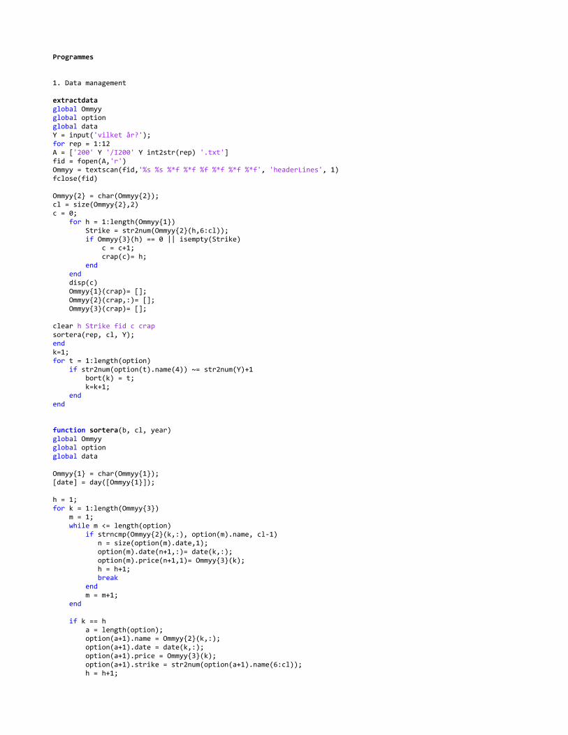
Programmes

1. Data management

extractdataglobal Ommyyglobal optionglobal dataY = input('vilket år?');for rep = 1:12A = ['200' Y '/I200' Y int2str(rep) '.txt']fid = fopen(A,'r')Ommyy = textscan(fid,'%s %s %*f %*f %f %*f %*f %*f', 'headerLines', 1)fclose(fid) Ommyy{2} = char(Ommyy{2});cl = size(Ommyy{2},2)c = 0; for h = 1:length(Ommyy{1}) Strike = str2num(Ommyy{2}(h,6:cl)); if Ommyy{3}(h) == 0 || isempty(Strike) c = c+1; crap(c)= h; end end disp(c) Ommyy{1}(crap)= []; Ommyy{2}(crap,:)= []; Ommyy{3}(crap)= []; clear h Strike fid c crapsortera(rep, cl, Y);endk=1;for t = 1:length(option) if str2num(option(t).name(4)) ~= str2num(Y)+1 bort(k) = t; k=k+1; endend

function sortera(b, cl, year)global Ommyyglobal optionglobal data Ommyy{1} = char(Ommyy{1});[date] = day([Ommyy{1}]); h = 1;for k = 1:length(Ommyy{3}) m = 1; while m <= length(option) if strncmp(Ommyy{2}(k,:), option(m).name, cl-1) n = size(option(m).date,1); option(m).date(n+1,:)= date(k,:); option(m).price(n+1,1)= Ommyy{3}(k); h = h+1; break end m = m+1; end if k == h a = length(option); option(a+1).name = Ommyy{2}(k,:); option(a+1).date = date(k,:); option(a+1).price = Ommyy{3}(k); option(a+1).strike = str2num(option(a+1).name(6:cl)); h = h+1;

endend a = size(option)clear s h k m n s1 = [year,char(64+b)]s2 = [year,char(76+b)]h = 1;g = 1;k = 1;for i =1:length(option) if option(i).name(4:5) == s1 data.(genvarname(s1))(h) = option(i); del(k) = i; k = k+1; h = h+1; elseif option(i).name(4:5) == s2 data.(genvarname(s2))(g) = option(i); del(k) = i; k = k+1; g = g+1; endend option(del) = [];b = size(option)

2. Calculations

impvol[TS] = TScreaterer(y);for month = 1:24 code = ['x' int2str(y),char(month+64)]; if month<13, exp = expiration(month,year,TS); else exp = expiration(month-12,year,TS); end for t = 1:length(data.(code)) omxprice = fts2mat(TS(data.(code)(t).date).OMXS30); ld = size(omxprice); strike = data.(code)(t).strike*ones(ld); time = (fts2mat(TS(exp).busday)-fts2mat(TS(data.(code)(t).date).busday))/250; value = data.(code)(t).price; if month<13, type = ones(ld); else type = zeros(ld); end for m = 1:ld(1) if time(m) <= 1/6 interest(m) = fts2mat(TS(data.(code)(t).date(m)).rf1m); elseif time(m) <= 1/4 interest(m) = fts2mat(TS(data.(code)(t).date(m)).rf2m); elseif time(m) <= 1/2 interest(m) = fts2mat(TS(data.(code)(t).date(m)).rf3m); elseif time(m) <= 3/4 interest(m) = fts2mat(TS(data.(code)(t).date(m)).rf6m); elseif time(m) <= 1 interest(m) = fts2mat(TS(data.(code)(t).date(m)).rf9m); else interest(m) = fts2mat(TS(data.(code)(t).date(m)).rf12m); end end interest = interest'; data.(code)(t).impvol = blsimpv(omxprice,strike,interest,time,value,[],[],[],type); clear interest disp(ld) endend

moneynessb = input('year?')a = b-1;s = ['OMX/OMX200' int2str(a) '.txt']fid = fopen(s,'r');omx = textscan(fid, '%s %*f %*f %f', 'headerLines',1);fclose(fid)

s = ['OMX/OMX200' int2str(b) '.txt']fid = fopen(s,'r');omx2 = textscan(fid, '%s %*f %*f %f', 'headerLines',1);fclose(fid)TS = fints([omx{1};omx2{1}],[omx{2};omx2{2}],'OMXS30'); for g = 65:88 s = ['x' int2str(b),char(g)] for i = 1:length(data.(s)) data.(s)(i).moneyness = data.(s)(i).strike./fts2mat(TS(data.(s)(i).date).OMXS30); endend

invimpvolfor h=65:88 code=['x1' char(h)] for i=1:length(data.(code)) mu=0; for j=1:length(data.(code)(i).impvol) if isnan(data.(code)(i).impvol(j)) || data.(code)(i).impvol(j)>45 mu=mu+1; elim(mu)=j; end end if mu >=1 data.(code)(i).date(elim)=[]; data.(code)(i).price(elim)=[]; data.(code)(i).moneyness(elim)=[]; data.(code)(i).impvol(elim)=[]; elim = []; end endend

calculationsfunction calculations(year)global data TS = TScreater([year,year-1],['1m ';'2m ';'3m ';'6m ';'9m ';'12m']);y = num2str(year); for month = 1:24 s = ['x' y,char(month+64)] if month<13 exp = expiration(month,year,TS); else exp = expiration(month-12,year,TS); end for k = 1:length(data.(s)) disp(k) OTS = fints(data.(s)(k).date,data.(s)(k).impvol,'iv'); omxprice = fts2mat(TS(data.(s)(k).date).OMXS30); ld = size(omxprice,1); strike = data.(s)(k).strike*ones(ld,1); time = (fts2mat(TS(exp).busday)-fts2mat(TS(data.(s)(k).date).busday))/250; volatility = fts2mat(OTS.iv); for m = 1:ld if time(m) <= 1/6 interest(m) = fts2mat(TS(data.(s)(k).date(m)).rf1m); elseif time(m) <= 1/4 interest(m) = fts2mat(TS(data.(s)(k).date(m)).rf2m); elseif time(m) <= 1/2 interest(m) = fts2mat(TS(data.(s)(k).date(m)).rf3m); elseif time(m) <= 3/4 interest(m) = fts2mat(TS(data.(s)(k).date(m)).rf6m); elseif time(m) <= 1 interest(m) = fts2mat(TS(data.(s)(k).date(m)).rf9m); else interest(m) = fts2mat(TS(data.(s)(k).date(m)).rf12m); end end

interest = interest'; t1 = log(omxprice./strike); t2 = interest.*time; t3 = volatility.^2./2.*time; n = volatility.*sqrt(time); d1 = (t1+t2+t3)./n; d2 = (t1+t2-t3)./n; d1star = (-t1+t2+t3)./n; d2star = (-t1+t2-t3)./n; st = FORM1(omxprice,d1,time); th = FORM2(interest,strike,time); clear m t1 t2 t3 n if month<13, data.(s)(k).delta = S(d1); else data.(s)(k).delta = S(d1)-1; end data.(s)(k).vega = V(omxprice,time,d1); if month<13, [data.(s)(k).theta,U] = blstheta(omxprice,strike,interest,time,volatility); else [U,data.(s)(k).theta] = blstheta(omxprice,strike,interest,time,volatility); end if month<13, [data.(s)(k).rho,U] = blsrho(omxprice,strike,interest,time,volatility); else [U,data.(s)(k).rho] = blsrho(omxprice,strike,interest,time,volatility); end data.(s)(k).gamma = blsgamma(omxprice,strike,interest,time,volatility); data.(s)(k).v2 = V2(volatility,d1,d2,data.(s)(k).vega); if month<13, data.(s)(k).t2 = T2(interest,time,volatility,d1,d2,d1star,d2star,th,st,'c'); else data.(s)(k).t2 = T2(interest,time,volatility,d1,d2,d1star,d2star,th,st,'p'); end data.(s)(k).sv = SV(volatility,d1,d2); data.(s)(k).st = ST(time,d1,d1star); data.(s)(k).vt = VT(d1,d1star,st); data.(s)(k).s3 = S3(omxprice,time,volatility,d1,data.(s)(k).gamma); data.(s)(k).v3 = V3(volatility,d1,d2,data.(s)(k).vega); % data.(s)(k).t3 = T3(volatility,d1,d2,data.(s)(k).theta); data.(s)(k).s2v = S2V(volatility,d1,d2,data.(s)(k).gamma); data.(s)(k).s2t = S2T(time,d1,d1star,data.(s)(k).gamma); data.(s)(k).sv2 = SV2(volatility,d1,d2); data.(s)(k).st2 = ST2(time,d1,d1star); data.(s)(k).v2t = V2T(volatility,d1,d2,d1star,d2star,st); data.(s)(k).vt2 = VT2(time,d1,d1star,st); data.(s)(k).svt = SVT(time,volatility,d1,d2,d1star,d2star); clear interest endend

function st = FORM1(P,d1,T)st=P.*normpdf(d1)./(2*sqrt(T));

function th = FORM2(R,S,T)th=R.*S.*exp(-R.*T);

function delta = S(d1)delta = normcdf(d1);

function dS2dT = S2T(T,d1,d1star,gamma)dS2dT = -gamma./(2*T).*(d1.*d1star+1);

function dS2dV = S2V(V,d1,d2,gamma)dS2dV = gamma./V.*(d1.*d2-1);

function dS3 = S3(P,T,V,d1,gamma)dS3 = (-gamma./P).*(d1./(V.*sqrt(T))+1);

function dSdT = ST(T,d1,d1star)dSdT = normpdf(d1).*d1star./(2*T);

function dSdT2 = ST2(T,d1,d1star)dSdT2 = normpdf(d1)./(4*T.^2).*(-d1.*d1star.^2+d1-2*d1star);

function dSdV = SV(V,d1,d2)dSdV = -normpdf(d1).*d2./V;

function dSdV2 = SV2(V,d1,d2)

dSdV2 = normpdf(d1)./V.^2.*(-d1.*d2.^2+d1+d2);

function dSdVdT = SVT(T,V,d1,d2,d1star,d2star)dSdVdT=normpdf(d1)./(2*T.*V).*(d1.*d2.*d1star-d2star);

function dT2 = T2(R,T,V,d1,d2,d1star,d2star,th,st,type)if type=='c' dT2 = V.*st.*(d1.*d1star+1)./(2*T)+th.*(-R.*normcdf(d2)+normpdf(d2).*d2star./(2*T));elseif type=='p' dT2 = V.*st.*(d1.*d1star+1)./(2*T)-th.*(-R.*normcdf(d2)+normpdf(d2).*d2star./(2*T));end

function vega = V(P,T,d1)vega = P.*sqrt(T).*normpdf(d1);

function dV2 = V2(V,d1,d2,vega)dV2 = vega.*d1.*d2./V;

function dV2dT = V2T(V,d1,d2,d1star,d2star,st)dV2dT = st./V.*(d1.*d2-d1.^2.*d2.*d1star+d2.*d1star+d2star.*d1);

function dV3 = V3(V,d1,d2,vega)dV3=vega./V.^2.*(d1.^2.*d2.^2-d1.^2-d2.^2-d1.*d2);

function dVdT = VT(d1,d1star,st)dVdT=st.*(1-d1.*d1star);

function dVdT2 = VT2(T,d1,d1star,st)dVdT2=-st./(2*T).*(-d1.^2.*d1star.^2+1+d1.^2+d1star.^2);

3. Forming samples

runglobal TSfor y=1:6 TScreater([y,y-1],['1m ';'2m ';'3m ';'6m ';'9m ';'12m']);eval(['load P0' int2str(y) '.mat']) for vecka = 2:13 boundary = [1.02,1.06]; holding = 5; eval(['C=sampcol(y,vecka,holding,boundary,P0' int2str(y) ')']) if isempty(C)==0 eval(['T=forecaster(C,y,vecka,P0' int2str(y) ')']) h = length(T); L = []; for i=1:h, if isempty(T{i})==0, for k=1:size(T{i},1),L(length(L)+1:length(L)+length(T{i}{k,1}),1)=T{i}{k,1};end,end,end L1 = []; for i=1:h, if isempty(T{i})==0, for k=1:size(T{i},1),L1(length(L1)+1:length(L1)+length(T{i}{k,2}),1)=T{i}{k,2};end,end,end L2 = []; for i=1:h, if isempty(T{i})==0, for k=1:size(T{i},1),L2(length(L2)+1:length(L2)+length(T{i}{k,3}),1)=T{i}{k,3};end,end,end L3 = []; for i=1:h, if isempty(T{i})==0, for k=1:size(T{i},1),L3(length(L3)+1:length(L3)+length(T{i}{k,4}),1)=T{i}{k,4};end,end,end eval(['X' int2str(y),'IV' int2str(vecka) '=[L,L1,L2,L3];']) endendclear global TSeval(['clear P0' int2str(y)])end

sampcolfunction C=reldates(year,vecka,holding,boundary,data)global TS C={};y = num2str(year);next=1;

for month = 1:12s = ['x' y,char(month+76)];exp = expiration(month,year);b = fts2mat(TS(exp).busday)-vecka*5;c = b+4;st = 0;bla = {};for k = 1:length(data.(s)) count=0; for loop = b:c OTS = fints(data.(s)(k).date,data.(s)(k).moneyness,'moneyness'); starting = TS.dates(loop); ending = TS.dates(loop+holding); if OTS.dates(1) <= starting && OTS.dates(length(OTS)) >= ending && isempty(OTS(datestr(starting)))==0 mnn = fts2mat(OTS(datestr(starting)).moneyness); if mnn >= min(boundary) && mnn < max(boundary) && isempty(OTS(datestr(ending)))==0 count = count+1; sdate(count,:)=datestr(starting); edate(count,:)=datestr(ending); end end end if count >=1 st = st+1; bla(st,:) = {k,sdate,edate}; clear sdate edate endendif isempty(bla)==0C{next,1}=s;C{next,2}=bla;next=next+1;endend

forecasterfunction T=statbuild(C,year,vecka,data)global TS if vecka/52 < 1/12 RF = 'rf1m'elseif vecka/52 < 1/6 RF = 'rf2m'elseif vecka/52 < 1/4 RF = 'rf3m'elseif vecka/52 < 1/2 RF = 'rf6m'end for i = 1:size(C,1) exp = expiration(i,year); A = C{i,1}; if isempty(C{i,2})==0 for k = 1:size(C{i,2},1) B = C{i,2}{k,1}; OTS = fints(data.(A)(B).date,[data.(A)(B).price,data.(A)(B).impvol],{'price','iv'}); OTS.delta = data.(A)(B).delta; OTS.vega = data.(A)(B).vega; OTS.theta = data.(A)(B).theta; OTS.rho = data.(A)(B).rho; OTS.gamma = data.(A)(B).gamma; OTS.v2 = data.(A)(B).v2; OTS.t2 = data.(A)(B).t2; OTS.sv = data.(A)(B).sv; OTS.st = data.(A)(B).st; OTS.vt = data.(A)(B).vt; OTS.s3 = data.(A)(B).s3; OTS.v3 = data.(A)(B).v3; OTS.s2v = data.(A)(B).s2v; OTS.s2t = data.(A)(B).s2t;

OTS.sv2 = data.(A)(B).sv2; OTS.st2 = data.(A)(B).st2; OTS.v2t = data.(A)(B).v2t; OTS.vt2 = data.(A)(B).vt2; OTS.svt = data.(A)(B).svt; ds = fts2mat(TS(C{i,2}{k,3}).OMXS30)-fts2mat(TS(C{i,2}{k,2}).OMXS30); dv = fts2mat(OTS(C{i,2}{k,3}).iv)-fts2mat(OTS(C{i,2}{k,2}).iv); dt = 1/250.*(fts2mat(TS(C{i,2}{k,2}).busday)-fts2mat(TS(C{i,2}{k,3}).busday)); dr = fts2mat(TS(C{i,2}{k,3}).(RF))-fts2mat(TS(C{i,2}{k,2}).(RF)); dO = fts2mat(OTS(C{i,2}{k,3}).price)-fts2mat(OTS(C{i,2}{k,2}).price); dO1 = fts2mat(OTS(C{i,2}{k,2}).delta).*ds+fts2mat(OTS(C{i,2}{k,2}).vega).*dv+fts2mat(OTS(C{i,2}{k,2}).theta).*dt+fts2mat(OTS(C{i,2}{k,2}).rho).*dr; dO2 = 1/2*(fts2mat(OTS(C{i,2}{k,2}).gamma).*ds.^2+fts2mat(OTS(C{i,2}{k,2}).v2).*dv.^2+fts2mat(OTS(C{i,2}{k,2}).t2).*dt.^2+2*fts2mat(OTS(C{i,2}{k,2}).sv).*ds.*dv+2*fts2mat(OTS(C{i,2}{k,2}).st).*ds.*dt+2*fts2mat(OTS(C{i,2}{k,2}).vt).*dv.*dt); dO3 = 1/6*(fts2mat(OTS(C{i,2}{k,2}).s3).*ds.^3+fts2mat(OTS(C{i,2}{k,2}).v3).*dv.^3+3*fts2mat(OTS(C{i,2}{k,2}).s2v).*ds.^2.*dv+3*fts2mat(OTS(C{i,2}{k,2}).sv2).*ds.*dv.^2+3*fts2mat(OTS(C{i,2}{k,2}).s2t).*ds.^2.*dt+3*fts2mat(OTS(C{i,2}{k,2}).st2).*ds.*dt.^2+3*fts2mat(OTS(C{i,2}{k,2}).v2t).*dv.^2.*dt+3*fts2mat(OTS(C{i,2}{k,2}).vt2).*dv.*dt.^2+6*fts2mat(OTS(C{i,2}{k,2}).svt).*ds.*dv.*dt); T{i}{k,1}=dO; T{i}{k,2}=dO1; T{i}{k,3}=dO2; T{i}{k,4}=dO3;

end endendT=T';

4. Analysis

grupperings=input('strike?');eval(['load P' s 'tmAll.mat'])for j=2:13 num=int2str(j) for k=1:6 eval(['exist X' int2str(k) s 'V' num ';']) if ans==0 eval(['X' int2str(k) s 'V' num '=[];']) end end eval(['ny=[X1' s 'V' num ';X2' s 'V' num ';X3' s 'V'... num ';X4' s 'V' num ';X5' s 'V' num ';X6' s 'V' num '];']) Ny1=abs(ny(:,1)-ny(:,2)); Ny2=abs(ny(:,1)-ny(:,2)-ny(:,3)); Ny3=abs(ny(:,1)-ny(:,2)-ny(:,3)-ny(:,4)); eval(['P' s 'V' num '=[ny(:,1),Ny1,Ny2,Ny3];']) end

analysfor i=2:13 for j=1:4 eval(['it=P' s 'V' int2str(i) '(:,' int2str(j) ');']) M(i,j)=mean(it); S(i,j)=std(it); end ss(i)=length(it); [a,b,c]=linreg([1:3],M(i,2:4)); regDM(i,:)=[a,b,c]; [a,b,c]=linreg([1:3],S(i,2:4)); regDS(i,:)=[a,b,c];endfor j=1:4 x=[2:13]'; [a,b,c]=linreg(x,M(2:13,j)); regTM(j,:)=[a,b,c];

[a,b,c]=linreg(x,S(2:13,j)); regTS(j,:)=[a,b,c];end

Linregfunction [a,b,r]=linreg(x,y)if length(x)~=length(y) disp('error') a=[];b=[];r=[];else n=length(x); Sxx=sum(x.^2)-1/n*sum(x)^2; Sxy=sum(x.*y)-1/n*sum(x)*sum(y); Syy=sum(y.^2)-1/n*sum(y)^2; b=Sxy/Sxx; a=sum(y)/n-b/n*sum(x); r=Sxy^2/Sxx/Syy;end

Acrosstrikesj=4;for i=2:13 a=['PIV' int2str(i)]; b=['PAV' int2str(i)]; c=['PO1V' int2str(i)]; d=['PO2V' int2str(i)]; col=['(:,' int2str(j) ')']; eval(['SM(i,:)=[mean(' a col '),mean(' b col '),mean(' c col '),mean(' d col ')];']) eval(['SS(i,:)=[std(' a col '),std(' b col '),std(' c col '),std(' d col ')];']) [a,b,c]=linreg([1:4],SM(i,:)); regSM(i,:)=[a,b,c]; [a,b,c]=linreg([1:4],SS(i,:)); regSS(i,:)=[a,b,c];end

lillieforss=input('strike');eval(['load ' s 'klar.mat'])for i=2:13 eval(['it=' s 'V' int2str(i) ';']) for j=2:4 eval(['ny=it(:,' int2str(j) ');']) lt(i,j)=lillietest(log(ny)); endend

nydessa = [8,10,11,12];for i=1:length(dessa) eval(['[m,h,t]=diffm(log(O2V' int2str(dessa(i)) '));']) tabell(i,:)=[m,h,t];end

diffmfunction [m,h,t]=diffm(samp)x=samp(:,4)-samp(:,3);n=length(x);m=mean(x);s=std(x);d=s/sqrt(n);u=m/d;t=tcdf(u,n-1);if t>0.975 h=1;else h=0;end

Documents

PANG InformationHigherOrderBSDerivative