Panel Stationarity Tests for Purchasing Power Paritywith Cross-sectional Dependence

David HarrisDepartment of EconomicsUniversity of Melbourne

Stephen Leybourne1

School of EconomicsUniversity of Nottingham

Brendan McCabeSchool of ManagementUniversity of Liverpool

30 August 2004

We investigate the purchasing power parity hypothesis for a group of 17 countries using a newpanel based test of stationarity that allows for arbitrary cross-sectional dependence. We treatthe short run time series dynamics non-parametrically and thus avoid the need to fit separate,and potentially misspecified, models for the individual series. The statistic is simple to computeand uses standard Normal critical values, even in the presence of a wide range of deterministiccomponents. We also show how the test can be applied using an approximate factor model forcross sectional dependence. Taken together, these features provide a generally applicable solutionto the problem of testing for stationarity versus unit roots in macro-panel based data. The testsfind significant evidence against the purchasing power parity hypothesis being true.

1Corresponding author, School of Economics, University of Nottingham, Nottingham NG7 2RD, UK. Email:steve.leybourne@nottingham.ac.uk

1

1 Introduction

Relatively long time series of many core macroeconomic variables are now available for the major-ity of developed economies. The use of panel data, and in particular unit root or stationarity tests,to empirically validate various important macroeconomic theories has become a rapid growth areaof applied econometric research. For example, panel tests have been used to assess the evidencefor the hypotheses of purchasing power parity (PPP), for convergence of growth rates, for meanreversion of inflation rates and for the real interest rate parity hypothesis. These tests attempt toexploit the potential power gains that are offered by analyzing a time series panel as opposed toindividual series and, as such, they have the potential to provide more compelling evidence for,or against, certain models of economic behaviour. Recent tests have been proposed by, inter alia,O’Connell (1998), Maddala and Wu (1999), Hadri (2000), Choi (2001, 2002), Chang and Song(2002), Levin, Lin and Chu (2002), Shin and Snell (2002), Chang (2003) and Im, Pesaran andShin (2003).

One of the major factors that any panel test needs to be able to address, if reliable inference isto be made in practical situations, is cross-sectional dependence. Cross-sectional dependencies arelikely to be the rule rather than the exception in studying cross-country data due to the existenceof strong inter-economy linkages. The tests of Hadri (2000), Choi (2001), Levin, Lin and Chu(2002), Shin and Snell (2002) and Im, Pesaran and Shin (2003) all assume independence acrossthe panel and their size properties are uncertain when this rather unrealistic assumption does nothold.2 The test of O’Connell (1998) allows for cross-sectional dependence, but this is restrictedto the innovation term driving an assumed finite order AR process in the model. Choi (2002)permits cross-sectional dependence but only after imposing a common additive error componentacross the panel. The testing approach adopted by Chang and Song (2002) provides, at leastin theory, a general treatment of the problem of cross-sectional dependence but their procedurerelies on user-supplied parameters, whose values are a function of the dependence structure itself,which rather limits its practical appeal. Maddala and Wu (1999) and Chang (2003) approachthe problem indirectly, relying on bootstrap procedures but the underlying tests are not pivotal.Regarding time series dynamics, with the exception of the test of Hadri (2000), all of these testsrely on fitting an appropriately specified time series regression model to each individual series inthe panel (a tedious and error prone undertaking unless the cross-sectional dimension is relativelysmall). For tests that allow cross-sectional dependence, this is a doubly vital requirement, as anynotion of these tests’ robustness to cross-sectional dependence is intimately reliant on the correctmodelling of the time series dynamics.

Recently, Bai and Ng (2004a,b) have suggested the use of an approximate factor model toaccount for cross sectional dependence in panel data. Their idea is to orthogonally decompose apanel of time series into a fixed number of independent common factors and remaining idiosyn-cratic components which are independent or weakly dependent. Bai and Ng (2004a,b) respectivelyconstruct Dickey-Fuller and KPSS tests for estimates of the unobserved components although theydo not explicitly provide tests for the observed series. While the performance of the Dickey-Fullerapproach may be deemed satisfactory, that of the KPSS procedure is much less so due to significantproblems with the size of the tests.

It would seem, then, that none of the extant approaches offers a totally satisfactory solutionto the problem of testing for stationarity, when the cross-sectional dependence structure and timeseries dynamics are both unknown. In contrast, the new stationarity test statistic we suggest inthis paper is constructed so as to overcome both these problems. We allow for arbitrary unknowncross-sectional dependence between the series in the panel; the series may be contemporaneously

2O’Connell (1998) shows that the test of Levin, Lin and Chu (2002) can suffer severe size distortions if appliedto panels where independence does not hold.

2

or cross-serially dependent. We also permit a wide range of heterogeneous stationary time seriesdynamics, which includes the conventional ARMA class.

Our statistic is based on a vector version of the stationarity test of Harris, McCabe andLeybourne (2003) (HML) (rather than a KPSS-type stationarity test as in Hadri (2000)). Thestatistic is, in essence, the sum of the lag-k sample autocovariances across the panel, suitablystudentized, where we allow k to be a simple increasing function of the time dimension. Bycontrolling k in such a way, we remove any need to explicitly model the time series dynamicsof each series in the panel, even though their time series dynamics may be quite heterogeneous.At the same time, the studentization automatically robustifies the statistic to the presence ofany form of cross-sectional dependence. Our statistic is simple to construct and, conveniently,possesses a limiting null distribution which is standard normal under quite general linear processassumptions.3 Asymptotic normality also holds when the statistic is calculated using residualsfrom deterministic regression models fitted to each series. These may include polynomial trendsor even structural breaks and there is no requirement that the same deterministic model be fittedto each series. As such, the test can be applied across a range of empirically relevant modellingsituations without reference to model-dependent null critical values, or the need to computebootstrap critical values. We also show how our new statistic can be applied to the factor modelshould such a model be deemed appropriate. The test, when applied to the factor model, is forstationarity of the observed series and has significantly more power than the original when thefactor model is correct. We also show how to construct a KPSS test for the observed series (asopposed to the components) in the factor model and compare its performance with the new testby means of some Monte Carlo experiments.

The plan of the paper is as follows. In the next section we introduce our statistic by explaininghow it can be used to distinguish between stationarity and unit roots in the panel context. Wealso derive its asymptotic properties and show how to incorporate deterministic regression effects.In Section 3 we show how our test may be applied to the observed series in the context of Baiand Ng’s (2004a) factor model. We also demonstrate how a KPSS test may be constructed forthe observed data. Section 4 reports the results of a number of Monte Carlo experiments togauge the empirical size and power of the tests. The results are very encouraging. In particular,the robustness of the new test’s size to different patterns of cross-sectional dependence and timeseries dynamics stands out as a prominent characteristic. In addition, there are useful powergains available by using our new statistic in combination with Bai and Ng’s (2004a) factor modelwhen appropriate. Finally, Section 5 assesses the evidence for PPP in a panel of US Dollar realexchange rates using the new test. We include the structural breaks version of PPP, as expoundedby Papell (2002), in the analysis and conclude by finding no evidence in favour of the hypothesis.

2 A Panel Test of Stationarity with Cross Sectional Correlation

Consider a panel of N time series zi,t, t = 1, ..., T generated by the processes

zi,t = φizi,t−1 + εi,t (1)

i = 1, 2, ..., N , t = 1, 2, ..., T

where each zero mean disturbance term εi,t, t = 1, ..., T is I (0) and εi,t and εj,t may be correlatedfor any i and j. Throughout, we considerN to be fixed and we shall let T grow in our limit theory.4

3Our asymptotics are based on a fixed cross-section dimension, and passing the time series dimension to infinity.For many macroeconomic applications, the assumption of a fixed cross-section dimension would appear reasonable.

4 It is possible to allows the number of observations to vary with the individual time series involved but we usea single T for notational convenience.

3

We wish to test the null hypothesis of joint stationarity

H0 : |φi| < 1 for all i

against the unit root alternative

H1 : φi = 1 for at least one i.

2.1 Motivation

To motivate our statistic, fix i and suppose for simplicity that εi,t, t = 1, ..., T in (1) is i.i.d. withvariance σ2i and, following Section 2.1 of HML, consider a test statistic for the variable zi,t basedon the scaled first order sample autocovariance Ci,1 = T−1/2

PTt=2 zi,tzi,t−1. Suitably centered and

studentized, this is the Dickey-Fuller statistic for testing the null hypothesis φi = 1. However,for testing H0 : |φi| < 1, the difficulty is that E (Ci,1) ' T 1/2σ2iφi/

¡1− φ2i

¢, so that the null

distribution depends on φi. We consider instead the corresponding kth order autocovariance

Ci,k = (T − k)−1/2TX

t=k+1

zi,tzi,t−k.

If k is chosen so that k →∞ and k/T → 0 as T →∞ then E (Ci,k) ' T 1/2σ2iφki /¡1− φ2i

¢→ 0 as

T →∞, so that the dependence of E (Ci,k) on φi disappears asymptotically. It is shown in Section5 of HML that Ci,k is asymptotically standard normal when suitably studentized and hence anydependence of the null distribution on φi (and σ2i ) is removed. When φi = 1, E (Ci,k) ' T 3/2σ2iand it can be shown the studentized statistic is divergent. Hence, for a single zi,t, a consistenttest with standard normal asymptotic null distribution can be based on Ci,k with k →∞.

To construct a joint test ofH0 : |φi| < 1 for all i, we follow the literature on panel Dickey-Fullertests and consider the sum of the individual test statistics

Ck =NXi=1

Ci,k.

Under H0, it is easily seen that

E [Ck] ' T 1/2NXi=1

σ2iφki /(1− φ2i )

and, setting k as before, E [Ck]→ 0 as T →∞ since N is fixed. This eliminates the dependence ofE (Ck) on all of the φi simultaneously. In fact Ck, when suitably studentized, has an asymptoticstandard normal distribution under H0. Under H1, suppose without loss of generality that φi = 1for i = 1, . . . , sN for some s ≤ 1 and |φi| < 1 for any i such that sN < i ≤ N . Then

E [Ck] ' T 3/2sNXi=1

σ2i + T 1/2NX

i=sN+1

σ2iφki /(1− φ2i ),

so that the leading right hand side term once more suggests that the test should be consistent.

4

2.2 The Test Statistic and its Distribution Theory

We assume that εt = (ε1,t, ..., εN,t)0 follows the stationary linear process assumption (Assumption

LP) of HML. This assumption permits cross-sectional correlation of any form between the seriesin the panel; this correlation may be contemporaneous or cross-serial. In addition, it allows forheterogeneity in the dynamics and variation across the panel. The series may exhibit a range ofindividual temporal dependence structures, including those of stationary ARMA processes.

Defining ak,t =PN

i=1 zi,tzi,t−k, the statistic Ck can be written Ck = T−1/2PT

t=k+1 ak,t. Thestudentized version of Ck is then given by

Sk =Ck

ω ak,t,

where ω2 at is the generic long-run variance estimator (LRV) of a sequence of variables a1, ..., aT :

ω2at = γ0at+ 2lX

j=1

µ1− j

l + 1

¶γjat, γjat = T−1

TXt=j+1

atat−j . (2)

Written this way, the statistic Sk can be seen to be the standardized mean of the constructed seriesak,t divided by its long run standard deviation, which provides some intuition for the followingresult.

Lemma 1 If the conditions of Theorems FCLT and LRV of HML hold and k = O¡T 1/2

¢then,

as T →∞,(i) Sk ⇒ N [0, 1] under H0,(ii) Sk diverges to +∞ under H1.

The Lemma is a special case of Theorem 1 below and so its proof is omitted. Theorems FCLTand LRV of HML impose conditions on the choice of k and l, the truncation parameter of theLRV. In this paper, we require k =

l(δT )1/2

mfor some constant δ > 0 and l/k → 0 as T →∞.

The role of the appropriate specification of k and ω2 ak,t is to remove the effects of thetemporal dependence in individual series from the asymptotic null distribution of Sk. SinceSk depends on zi,t and zi,t−k only through the cross section sum ak,t =

PNi=1 zi,tzi,t−k, any

valid estimate of the long run variance of ak,t will automatically correct for any pattern ofcross sectional dependence in zi,t. Hence, there is no need to parametrically model the dynamicstructure of each series or their cross-sectional dependencies. A similar LRV approach is adoptedby Driscoll and Kraay (1998) to GMM inference for panel data with cross sectional dependencebut without the added complication of k→∞.

2.3 Deterministic Regression Effects

The statistic Sk is generally not feasible because in practice each zi,t will be estimated from aregression on some deterministic terms. Such vectors of deterministics are denoted xi,t and maybe different for each i if required. In place of (1), we consider the model given by

yi,t = β0ixi,t + zi,t. (3)

zi,t = φizi,t−1 + εi,t

i = 1, 2, ..., N , t = 1, 2, ..., T.

Let zi,t denote an OLS residual from the regression (3) i.e. zi,t = yi,t− β0ixi,t where βi is the usual

OLS estimator. It is desirable that the statistic be invariant to relative rescaling of the series, so

5

in place of zi,t in the definition of Sk we will use instead the standardized residuals

zi,t = zi,t/si, (4)

where si is the sample standard deviation of zi,t. The resulting statistic is

Sk =Ck

ω ak,t

where Ck = T−1/2PT

t=k+1 ak,t and ak,t =PN

i=1 zi,tzi,t−k.

It can be shown that Sk has an asymptotic standard normal null distribution and, whendealing with a small number of series, this often proves to be an adequate approximation for thefinite sample distribution. However, if the panel dimension is not relatively small, individual finitesample errors that arise from the estimation of the regression models combine in the constructionof the aggregate numerator Ck =

PNi=1 Ci,k and can significantly affect the finite sample null

distribution of Sk. To see how this arises, write the numerator of Sk as Ck =PN

i=1 Ci,k whereCi,k = T−1/2

PTt=k+1 zi,tzi,t−k . After some manipulation, Ci,k may be expressed as

Ci,k =1

s2iT−1/2

TXt=k+1

zi,tzi,t−k

−T−1/2⎡⎣ 1s2iT−1/2

TXt=1

zi,tx0i,t

ÃT−1

TXt=1

xi,tx0i,t

!−1T−1/2

TXt=1

xi,tzi,t

⎤⎦+ op(T−1/2) (5)

The first term in this expression is asymptotically normal under the null and the effect of theregression estimation error is captured by (5). Under H0, the term in square brackets in (5) isOp(1) and so the whole term is Op(T

−1/2). Because the term (5) is clearly negative it inducesa negative finite sample error into each individual statistic and the amplification of this problemis obvious when we subsequently consider Ci,k summed over N . Since we are conducting uppertail tests, ceteris paribus, the effect of this is to reduce the finite sample size of the test5. It ispossible to produce a finite sample correction for this regression estimation error by subtractingan estimate of the term (5) from Ci,k. It is shown in the proof of Theorem 1 below that theexpectation of the term in square brackets in (5) can be consistently estimated by

ci = tr

⎡⎣ÃT−1 TXt=1

xi,tx0i,t

!−1Ωxi,tzi,t

⎤⎦ (6)

where for any vector sequence a1, ..., aT ,

Ωat = Γ0at+lX

j=1

µ1− j

l + 1

¶³Γjat+ Γjat0

´, Γjat = T−1

TXt=j+1

ata0t−j . (7)

This is the usual matrix version of the scalar long run variance ω .2. Specializing to the caseof a constant, xi,t = 1, we can compute ci = ωzit2 and in the case of xi,t = [1, wi,t]

0, ci =ωzit2 + ωzitwi,t2 where wi,t = (wi,t − wi) /sw,i and sw,i is the standard deviation of thevariable wi,t.

5Simulation results, available from the authors, emphatically confirm this for moderate values of N and T .

6

To summarize, our recommended statistic for application is

Sk =Ck + c

ω ak,t(8)

where c = (T − k)−1/2PN

i=1 ci, ci is given in (6), Ck = (T − k)−1/2PT

t=k+1 ak,t where ak,t =PNi=1 zi,tzi,t−k and zi,t is obtained from (4) and ω ak,t is obtained from (2). The proof of the

following theorem is given in the Appendix.

Theorem 1 If the conditions of Theorem RES of HML hold and k = (δT )1/2 (for some constantδ > 0) then as T →∞(i) Sk ⇒ N (0, 1) under H0,(ii) Sk diverges to +∞ under H1.

Theorem RES of HML specifies quite general conditions on xi,t, allowing for a wide range of deter-ministic regression functions including constants, linear and polynomial trends, dummy variables,structural breaks and various other models. The theorem shows that a consistent test is obtainedby rejectingH0 for values of Sk greater than the appropriate upper tail critical value from the stan-dard normal distribution. We implement the test in Sections 4 and 5 using l =

l12 (T/100)1/4

min ω ak,t and k =

l(3T )1/2

m.

3 Panel Tests for Stationarity in Factor Models

An alternative approach to panel stationarity testing in the presence of cross sectional correlationis based on the factor model of Bai and Ng (2004a,b). Instead of the nonparametric model (1),consider the factor model

yi,t = µi + zi,t, (9)

zi,t = λ0ift + ei,t, (10)

where µi is a constant term6, ft is an r× 1 vector of latent factors, λi is an r× 1 vector of loading

parameters and ei,t is an idiosyncratic component for each i. It is assumed that ft = (f1,t, . . . , fr,t)0

and ei,t satisfy

fj,t = αjfj,t−1 + uj,t, j = 1, . . . , r, (11)

ei,t = ρiei,t−1 + vi,t, i = 1, . . . , N, (12)

for t = 1, . . . , T , where uj,t, t = 1, ..., T and vi,t, t = 1, ..., T are mutually independent I (0)disturbances7 for all i and j.

Bai and Ng (2004a) give a detailed analysis of the estimation of the unobserved componentsfj,t and ei,t by principal components, showing that it is necessary to carry out the principal com-ponents analysis on ∆zi,t rather than zi,t for consistent estimation under both null and alternativehypotheses8. To briefly summarize their estimation method, let ∆Y be the (T − 1)×N matrix ofobservations on ∆yi,t and let d∆F be the (T − 1)× r matrix of eigenvectors corresponding to the

6Other deterministic components may be included, with some complications noted below.7The asymptotic theory of the tests based on this model allows weak correlation among uj,t and εi,t, see

Assumption C of Bai and Ng (2004a). Independence is maintained here for ease of interpretation and is imposedin the simulations below.

8 In contrast to our asymptotic theory for the Sk test, this consistency follows as both N and T go to infinity.Although this consistency is not required for our results, we adopt their estimation strategy as it provides a testwith good finite sample properties.

7

largest r eigenvalues of ∆Y∆Y 0 (i.e. the r largest principal components of ∆Y ). The estimatedidiosyncratic components d∆E in first difference form are the residuals from an OLS regressionof ∆Y on d∆F . Letting d∆fj,t and d∆ei,t denote the individual elements of d∆F and d∆E respec-tively, the estimated components are found by partial summation, that is fj,t =

Pts=2

d∆fj,s andei,t =

Pts=2

d∆ei,s for t = 2, . . . , T (j = 1, . . . , r and i = 1, . . . , N ). Since r is unknown in practice,it is estimated using the Bai and Ng (2002) BIC type criterion

r = arg min0≤r≤rmax

½log σ2 (r) + r log

µNT

N + T

¶µN + T

NT

¶¾(13)

where σ2 (r) = (NT )−1PT

t=2

PNi=1 e

2i,t to give an estimate of r. Bai and Ng (2002) prove consis-

tency of r when r ≤ rmax and N,T →∞.Bai and Ng (2004a) construct unit root tests for the estimated components and Bai and

Ng (2004b) provide stationarity tests based on the well known univariate stationarity test ofKwiatkowski, Phillips, Schmidt and Shin (1992, KPSS). By testing the unit root or stationarityproperties of the components rather than the observable series, Bai and Ng are able to avoid theproblems arising from cross sectional correlations among the series and to deduce much detailedinformation about the time series properties of the panel. However, in this paper we aim to finda single test for the null hypothesis that the series zi,t, t = 1, ..., T are stationary for all i.

The null hypothesis for the panel stationarity test based on (9)—(12) is

H0 : |αj | < 1, |ρi| < 1 for all i, j,

against the alternative hypothesis

H1 : αj = 1 for at least one j and/or ρi = 1 for at least one i.

The approach is apply a stationarity test to all of the estimated components jointly.

3.1 A Stationarity Test for the Estimated Components

The Sk test can be calculated for the estimated components fj,t and ei,t. Let fj,t and ei,t denotefj,t and ei,t each individually demeaned and standardized to have unit standard deviation. Thestatistic (8) can be calculated for these standardized estimated components by redefining zi,t to

be the ith element of the (N + r)×1 vector³f1,t, . . . , fr,t, e1,t, . . . , eN,t

´0and the resulting statistic

is denoted SFk . The asymptotic properties of S

Fk follow from Theorem 2 below, which shows that

a consistent test is obtained by rejecting H0 for values of SFk greater than the appropriate upper

tail critical value from the standard normal distribution.Equation (9) can be extended to a general deterministic regression of the form

yi,t = β0ixi,t + zi,t. (14)

This deterministic formulation extends that of Bai and Ng (2004a) who allowed only for a constantand trend. For example, xi,t in Section 5 contains trend functions with structural breaks whosedates differ for each i. The computation of SF

k is outlined where xi,t = xt for all i, while detailsof how to handle fully general deterministic terms are available in Appendix 6.2. The estimationof the factor model (14), (10)—(12) in first differences begins with the estimation of the OLSregressions of ∆yi,t on ∆xt9 for each i = 1, . . . , N to obtain residuals ∆zi,t which are arranged inthe (T − 1)×N matrix d∆Z. Equation (10) is estimated by principal components as discussed in

9 If xt contains a constant then the corresponding element of ∆xt is deleted.

8

the previous section, with ∆Y replaced byd∆Z. The resulting estimated components, fj,t and ei,tfor j = 1, . . . , r and i = 1, . . . , N are individually regressed on xt to give residuals which are eachstandardized to have unit variance. Again zi,t is redefined to be the ith element of the (N + r)×1vector

³f1,t, . . . , fr,t, e1,t, . . . , eN,t

´0of standardized residuals, and the statistic (8) is calculated

from this vector to give SFk .

Theorem 2 Under the conditions of Theorem 1,(i) SF

k ⇒ N (0, 1) under H0,(ii) SF

k diverges to +∞ under H1.

Note that the theorem is proved for general deterministic regressions as outlined in Appendix6.2. It follows essentially because SF

k is computed on a linear transformation (determined bythe principal components analysis) of the observed data, provided the linear transformation isappropriately de-trended. The asymptotic theory is not informative about the relative merits ofSFk and Sk, but the simulations in Section 4 reveal that SF

k has superior finite sample power inthe factor model.

3.2 A KPSS Test for the Estimated Components

A point of comparison for the SFk and Sk tests is provided by a simple adaptation of the pooled

KPSS test of Bai and Ng (2004b)10. It is also a variation of Hadri (2000) where the pooled KPSStest was applied directly to yi,t assuming no cross sectional correlation. For the factor model(9)—(12), let fj,t and ei,t be standardized versions of fj,t and ei,t obtained from the principalcomponents estimation. The individual KPSS statistics for the estimated components are

ηf,j =T−2

PTt=2

³Pts=2 fj,s

´2ω2nfj,t

o , ηe,i =T−2

PTt=2

¡Pts=2 ei,s

¢2ω2 ei,t

for j = 1, . . . , r and i = 1, . . . , N . The pooled test of H0 : |αj | < 1, |ρi| < 1 for all i, j is

ηµ =1

c2√N + r

⎛⎝ rXj=1

¡ηf,j − c1

¢+

NXi=1

¡ηe,i − c1

¢⎞⎠ (15)

where c1 = 0.167 and c2 = 0.149 are asymptotic constants whose values are taken from Hadri(2000). The µ subscript denotes the inclusion of a constant in (9). It follows from Theorem 1 ofBai and Ng (2004b) and Theorem 1 of Hadri (2000) that ηµ has an asymptotic standard normalnull distribution as N and T approach infinity. Under the alternative, those individual statisticscorresponding to nonstationary components diverge to +∞, so the pooled test is defined to rejectthe null when ηµ is larger than the appropriate upper tail critical value from the standard normaldistribution.

The consistency of the test when both N and T approach infinity requires consideration. Ifan individual component (fj,t or ei,t) is I (1) then its corresponding statistic diverges to +∞ atrate11 Op (T/l) where l is the bandwidth parameter in the long run variance ω2 .. If any of10Bai and Ng (2004b) provide a test of the stationarity of the individual factors and a separate pooled test for the

idiosyncratic components, but testing the components separately obviously introduces a multiple testing problemfor our null.11This follows from the consistency of the component estimates under the alternative shown by Bai and Ng

(2004a) and then from the well known divergence rate of the KPSS statistic.

9

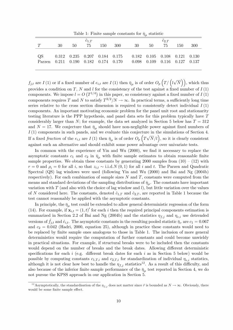
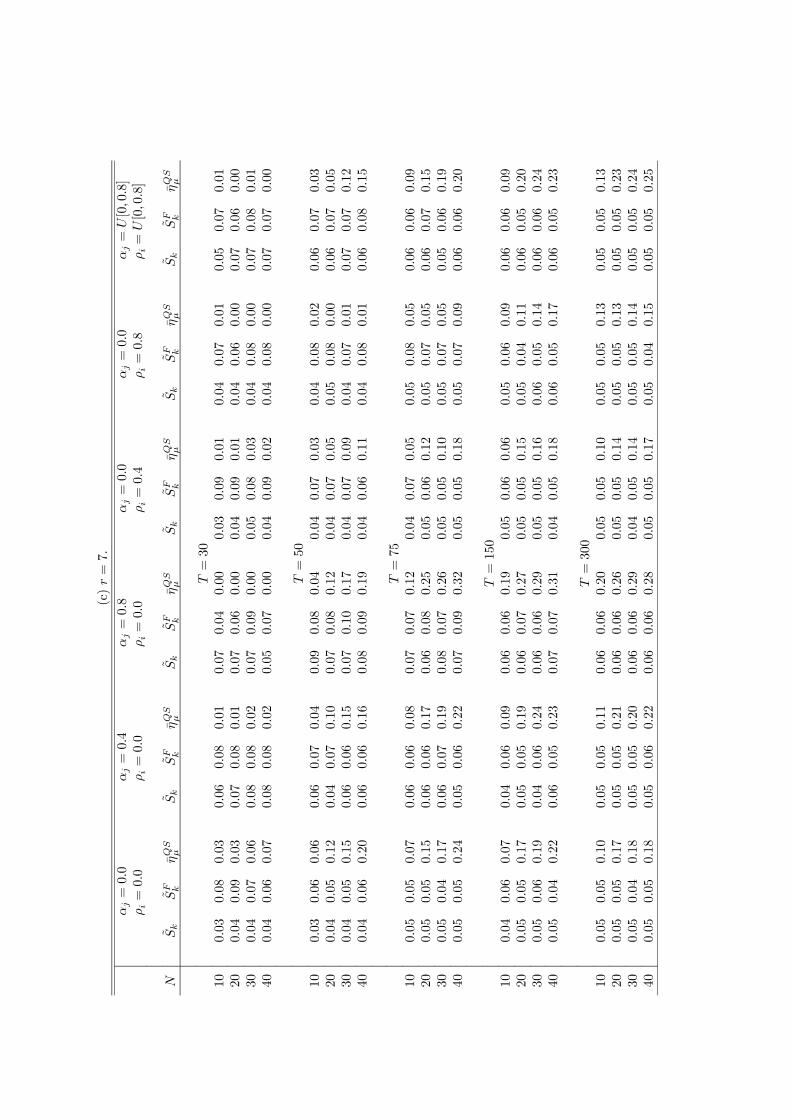
Table 1: Finite sample constants for ηµ statistic

c1,T c2,TT 30 50 75 150 300 30 50 75 150 300

QS 0.312 0.235 0.207 0.184 0.175 0.182 0.105 0.108 0.121 0.130Parzen 0.211 0.190 0.182 0.174 0.170 0.098 0.109 0.116 0.127 0.137

fj,t are I (1) or if a fixed number of ei,t are I (1) then ηµ is of order Op

³T/³l√N´´, which thus

provides a condition on T , N and l for the consistency of the test against a fixed number of I (1)components. We impose l = O

¡T 1/4

¢in this paper, so consistency against a fixed number of I (1)

components requires T and N to satisfy T 3/2/N →∞. In practical terms, a sufficiently long timeseries relative to the cross section dimension is required to consistently detect individual I (1)components. An important motivating economic problem for the panel unit root and stationaritytesting literature is the PPP hypothesis, and panel data sets for this problem typically have Tconsiderably larger than N ; for example, the data set analyzed in Section 5 below has T = 312and N = 17. We conjecture that ηµ should have non-negligible power against fixed numbers ofI (1) components in such panels, and we evaluate this conjecture in the simulations of Section 4.

If a fixed fraction of the ei,t are I (1) then ηµ is of order Op

³T√N/l

´, so it is clearly consistent

against such an alternative and should exhibit some power advantage over univariate tests.In common with the experience of Yin and Wu (2000), we find it necessary to replace the

asymptotic constants c1 and c2 in ηµ with finite sample estimates to obtain reasonable finitesample properties. We obtain these constants by generating 2000 samples from (10) — (12) withr = 0 and ρi = 0 for all i, so that zi,t ∼ i.i.d.N (0, 1) for all i and t. The Parzen and QuadraticSpectral (QS) lag windows were used (following Yin and Wu (2000) and Bai and Ng (2004b)respectively). For each combination of sample sizes N and T , constants were computed from themeans and standard deviations of the sampling distributions of ηµ. The constants have importantvariation with T (and also with the choice of lag window and l), but little variation over the valuesof N considered here. The constants, denoted c1,T and c2,T , are reported in Table 1 because thetest cannot reasonably be applied with the asymptotic constants.

In principle, the ηµ test could be extended to allow general deterministic regression of the form(14). For example, if xi,t = (1, t)

0 for each i then the required principal components estimation issummarized in Section 2.2 of Bai and Ng (2004b) and the statistics ηf,j and ηe,i use detrendedversions of fj,t and ei,t. The asymptotic constants in the resulting pooled statistic ητ are c1 = 0.067and c2 = 0.042 (Hadri, 2000, equation 25), although in practice these constants would need tobe replaced by finite sample ones analogous to those in Table 1. The inclusion of more generaldeterministics would require the computation of further constants and could become unwieldyin practical situations. For example, if structural breaks were to be included then the constantswould depend on the number of breaks and the break dates. Allowing different deterministicspecifications for each i (e.g. different break dates for each i as in Section 5 below) would bepossible by computing constants c1,T,i and c2,T,i for standardization of individual ηe,i statistics,although it is not clear how best to handle the ηf,j statistics

12. As a result of this difficulty, andalso because of the inferior finite sample performance of the ηµ test reported in Section 4, we donot pursue the KPSS approach in our application in Section 5.

12Asymptotically, the standardisation of the ηf,j does not matter since r is bounded as N →∞. Obviously, therewould be some finite sample effect.

10

3.3 Comparison of the two approaches

A theoretical difference between testing via Sk (or SFk ) and ηµ is that Sk and S

Fk use an asymptotic

approximation with T →∞ and N fixed, while ηµ uses both T and N approaching infinity. Weconsider the resulting difference in interpretation of how each approach handles the cross sectionalcorrelation.

Since Sk holds N fixed, it may be regarded as being parametric with respect to cross sectionalcorrelation since there are a fixed number (N (N − 1) /2) of correlations13. However, these cor-relations have no structure imposed upon them so the approach is otherwise completely flexible.Any lagged cross correlations between individual series are modelled nonparametrically withinthe multivariate linear process assumption (HML, Assumption LP) and their effects on the teststatistic are implicitly catered for by the long run variance in the denominator.

Since ηµ is based upon a factor model with a fixed number of factors, it may also be regardedas being parametric with respect to the cross sectional correlation, although there is also a non-parametric aspect to the approach since the factor loadings are unrestricted for each i = 1, . . . , N .The requirement that N →∞ is important for the consistent estimation of the factors and idio-syncratic components in model (9). Compared to Sk and SF

k , we believe the parametric aspectof the ηµ test imposes the more restrictive assumption because model (9) can potentially be mis-specified if insufficient factors are included or if a factor model is inappropriate. Note that SF

k

remains valid in the presence of misspecification of the factor model. We include some simulationsin Section 4 that address the possible practical consequences of such a misspecification.

4 Finite Sample Properties

In this section we report the results of a simulation experiment to evaluate the finite sampleproperties of the three tests considered in this paper. To our knowledge there is no other existingpanel test for stationarity that is valid in the presence of cross sectional correlation that canbe included in the experiment. All experiments include a constant term in the deterministicspecification.

For all experiments the data generating process is the factor model (9) — (12) with disturbances(u1,t, . . . , ur,t, ε1,t, . . . , εN,t)

0 drawn from the N (0, IN+r) distribution. The sample sizes are N =10, 20, 30, 40 and T = 30, 50, 75, 150, 300, which are chosen to include realistic sample sizes formacroeconometric applications. The number of factors included are r = 0, 2 and 7. The estimationof the factor model is implemented using rmax = 6 when choosing the number of factors, so thefactor model can be correctly specified when r = 0 or 2, but is misspecified when r = 7. Weinclude the r = 7 case to give some idea of the consequences of misspecifying the factor model,which in practice could be due to underspecification of the number of factors or to a model witha fixed number of factors being inappropriate. There is no cross sectional correlation when r = 0.When r = 2, 7 we consider λi ∼ i.i.d.N

¡κ, κ2

¢(fixed across replications) with κ = 3, which is the

same as used by Bai and Ng (2004b) except for the multiplicative constant κ. Since uj,t and εi,tare standard normal variates, κ is used to control the relative standard deviations of the factorscompared to the idiosyncratic components. The value of κ turns out to be unimportant for r = 2,but is important for r = 7 when the factor model is misspecified because it determines the relativemagnitude of the factor14 that is omitted. The choice of κ = 3 is within the range of empiricalstandard deviation ratios reported in Table 4 of Bai and Ng (2004b) for a panel of quarterly real13We conjecture that the approach remains valid if N → ∞ sufficiently slowly as T → ∞, and hence may be

classed fully nonparametric, but we defer this technical issue for other research.14We find that r = 6 in every replication in this case, so one factor can be considered to be omitted. Obviously

finding r = rmax in practice would lead to some model respecification, with at least an increase in rmax. The pointhere is to evaluate the effect of a model misspecification.

11

exchange rates. Predictably, unreported simulations reveal that the consequences of the modelspecification are worse when κ is increased from 3, and better when κ is decreased.

After preliminary experimentation, we implement the Sk and SFk statistics using k =

l(3T )1/2

mand the long run variances are estimated using a Bartlett lag window with l =

l12 (T/100)1/4

m.

Following Bai and Ng (2004b), the long run variances are computed using the Quadratic Spectral15

lag window with l =l12 (T/100)1/4

mgiving ηQSµ .

All tests are taken to reject the null hypothesis at the 5% significance level when the teststatistic is larger than 1.65. All experiments use 5000 replications.

4.1 Size

Under the null hypothesis, the values of αi and ρj in (11) and (12) considered are (αj , ρi) = (0, 0),(0.4, 0), (0.8, 0), (0, 0.4), (0, 0.8) for all i and j. Any difference in the effect of autocorrelation inthe factors and idiosyncratic components can be evaluated. We also consider αj and ρi drawn fromindependently from a U [0, 0.8] distribution for all i and j (fixed across replications) to includesome heterogeneity across the components.

Table 2(a) contains estimated finite sample sizes for r = 0; the case of no cross-correlation.The results for ρi = 0 reveal actual sizes near to the asymptotic 0.05 level. The only exceptionis some mild oversizing for the Sk and SF

k tests for T = 30, although it is not surprising that anasymptotic approximation based on T → ∞ with N fixed is not very accurate when T is smalland N is about the same magnitude. Increasing ρi to introduce idiosyncratic autocorrelationreveals that Sk and SF

k are well behaved for ρi = 0.4 and somewhat undersized for small T andρi = 0.8. The η

QSµ test is undersized for ρi = 0.4 and small T and displays a worrying mixture of

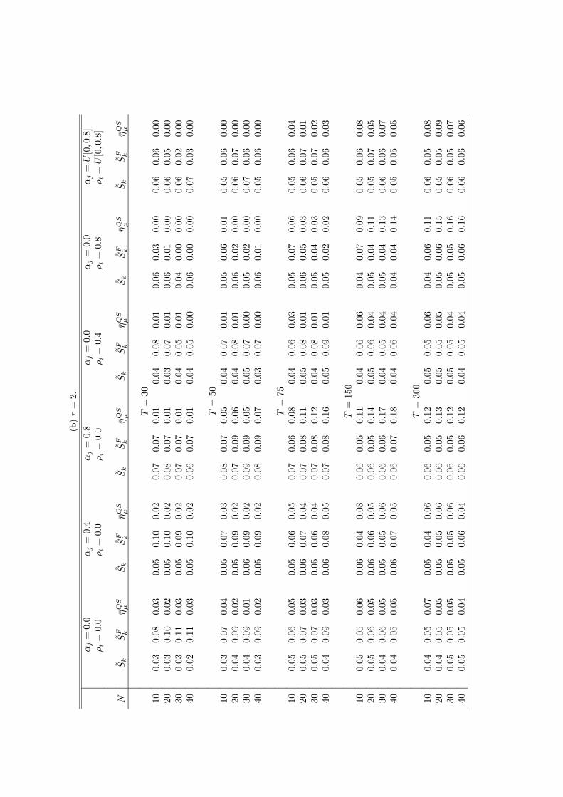
undersizing and oversizing when ρi = 0.8.Table 2(b) gives the results for the cross-correlated case where r = 2. The Sk and SF

k testshave good size properties in all cases and quickly approach correct levels for realistic macro-economic sample sizes. The ηQSµ is somewhat undersized for small T in the presence of strongautocorrelation, then becomes oversized as T increases, even with T = 300.

Table 2(c) gives the results for r = 7. The properties of Sk and SFk are essentially the same

as for r = 2, illustrating the robustness to cross correlation and factor model misspecificationof these tests. The interest is in ηQSµ since it relies on the correct specification of the model –across all values of the autoregressive parameters, it is clear that ηQSµ becomes progressively veryoversized as T increases. This gives some quantitative idea of the possible price of relying on amisspecified model for this testing problem.

In summary, it is clear that Sk and SFk provide generally much superior finite sample size

properties across a range of data generating processes.

4.2 Power

Under the alternative hypothesis, we set ρi = 1 for i = 1, . . . , sN and ρi = 0 for i = sN+1, . . . , Nwhere s = 0.1, 0.2, 0.4 and 0.6. When r = 2, we also consider an alternative of the formα1 = α2 = 1 with ρi = 0 for all i. Results for r = 7 are not reported for brevity and sincethe model for computing ηQSµ is misspecified and size control for that test is poor. Powers arereported in Table 3. Table 4 reports size adjusted powers (using the finite sample critical valuescalculated with s = 0 and α1 = α2 = 0 in the case of r = 2), which may have some theoreticalinterest but very limited practical relevance since they are based on infeasible tests.

15Unreported simulations show the Parzen lag window suggested by Yin and Wu (2000) for the test of Hadri(2000) to be inferior to the QS lag window in this case.

12

Table 3(a) reports powers for the non cross-correlated case r = 0. The results for Sk and SFk

reveal power increasing with T as expected, and interestingly power also increasing with N . Thepattern is similar for ηQSµ , although the effect of increasing N is not as uniform. Table 2(a) showsthe sizes of all three tests for ρi = 0 are very similar for T = 150 and 300, so comparing powersfor these sample sizes reveals a considerable power advantage for the Sk and SFk tests. There islittle difference between these latter two tests.

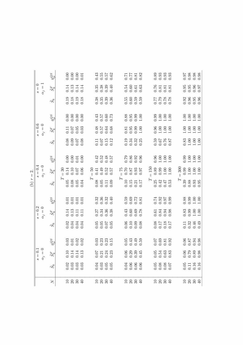
Table 3(b) reports powers for r = 2, and shows a significant change from the results in Table3(a). The Sk test is now least powerful by some margin against idiosyncratic unit roots while SF

k

is occasionally most powerful and ηQSµ is frequently most powerful. The Sk test does, however,have highly competitive against common factors with unit roots (the s = 0, αj = 1 alternative).Overall though, these results show a clear power advantage for SF

k over Sk, so it is well worth thepreliminary estimation of the factor model to calculate SF

k . The size adjusted powers in Table 4again confirm the superiority of SF

k over Sk when r = 2.Overall, the size and power results show SF

k to be the preferred panel stationarity test forfactor models. The Sk has good size properties but inferior power against idiosyncratic unitroots in the presence of stationary common factors. The ηQSµ test has poor size control in thepresence of strongly autocorrelated idiosyncratic components in any model and is susceptible tomisspecification of the factor model, so it cannot be recommended for use from this comparison.

5 Testing the Purchasing Power Parity Hypothesis

In this section, we empirically test the purchasing power parity hypothesis, which is a fundamentalingredient of macroeconomic models of bilateral exchange rate behaviour. The validity of the PPPhypothesis has been an issue that has attracted a vast amount of attention in recent times andhas been tested extensively using different panel unit root tests. In general, little evidence insupport of PPP has been uncovered. For example, Papell (1997), Cheung and Lai (2000), Wuand Wu (2001) and Chang and Song (2002) are unable to provide strong evidence against the unitroot null.16 A failure to reject this null does not, however, provide compelling evidence againstthe PPP hypothesis, not least because low test power may be an issue here since real exchangerates tend to be highly correlated as they are typically constructed using a common numerairecurrency and price index. Conversely, even if a rejection of the unit root null were to be obtained,this could not be interpreted as evidence for PPP holding in the entire panel because it may bethat only a subset of the real exchange rates are stationary. In view of this, it makes some senseto apply our panel stationarity tests, Sk and SF

k , in this context. Here, the PPP hypothesis isrepresented by the stationary null and a rejection can, ceteris paribus, fairly unambiguously beinterpreted as evidence against the PPP hypothesis being true.

We consider monthly real exchange rates against the US Dollar for the following countries:Austria, Belgium, Canada, Denmark, Finland, France, Germany, Greece, Italy, Japan, Nether-lands, Norway, Portugal, Spain, Sweden, Switzerland and the UK. The real exchange rate datawas constructed from raw nominal exchange rate and consumer price index data taken from theIMF International Financial Statistics database. It covers the period of the recent float, 1973.01to 1998.12. We have N = 17 and T = 312. In our notation we take yi,t to be the natural log ofthe real exchange rate, each standardized to have unit variance17.

16 In fact, what little empirical evidence there is in support of PPP has mainly arisen from application of teststhat do not account for cross-sectional dependence at all; see Oh (1996) and Wu (1996).17The data files and Gauss program for this application may be downloaded from

www.economics.unimelb.edu.au/dharris

13

5.1 PPP with a Mean

As usual in PPP analysis, we first hypothesize that yi,t has a constant mean represented by

yi,t = µi + zi,t,

where the null hypothesis of PPP requires that zi,t is I (0) and the alternative hypothesis is thatzi,t is I (1). The Sk test statistics for each of the 17 series individually (i.e. each test has N = 1)are given in Table 5 under the “Constant” heading, together with the p-value of each test. Atthe 0.05 and 0.10 levels, the null hypothesis is rejected for 4 and 10 countries respectively, so theevidence against PPP is mixed.

The panel Sk statistic pooled across the 17 countries gives Sk = 1.93 (p = 0.027). The esti-mation of the factor model (9)—(12), for this data, gives r = 2 when rmax = 5, and the resultingtest statistic is SF

k = 3.75 (p = 0.000). Thus the panel tests clearly reject the null hypothesis ofPPP.

5.2 PPP with Structural Breaks

Papell (2002) suggests that rejections of PPP, such as that we have just found, are due to anunusual one-off episode in the 1980’s when there was a large unexplained appreciation of the USdollar followed by an equally large offsetting depreciation. In econometric terms, this translatesto a generalization of the deterministic specification so that

yi,t = µi,t + zi,t, (16)

where

µi,t =

⎧⎪⎪⎨⎪⎪⎩β1,i, t ≤ τ1,i,β2,i + β3,it, τ1,i ≤ t ≤ τ2,i,β4,i + β5,it, τ2,i ≤ t ≤ τ3,i,β1,i, τ3,i ≤ t,

(17)

and all the βj,i and τ j,i have to be estimated. Papell (2002) suggests that PPP holds around aconstant long run real exchange rate before break point τ1,i and after break point τ3,i; note thatthe same mean, β1,i, applies in these two time periods and that this restriction is imposed onour test. The middle two time periods correspond to the great appreciation (τ1,i ≤ t ≤ τ2,i) andthe great depreciation (τ2,i ≤ t ≤ τ3,i). The null hypothesis of PPP in this setting is that yi,t hasrepresentation (16) where µi,t satisfies (17) and zi,t is I (0).

As in Papell (2002), note that the representation of µi,t in (17) is constrained to be continuousin t and it is therefore convenient to reparameterize µi,t as

µi,t = α1,i + α2,ix1,i,t + α3,ix2,i,t + α4,ix3,i,t,

where for h = 1, 2, 3xh,i,t = (t− τh,i) · 1 (t > τh,i) ,

subject to the additional restrictions that α2,i + α3,i + α4,i = 0 (so that there is no trend fort > τ3,i) and α2,i (τ3,i − τ1,i) + α3,i (τ3,i − τ2,i) (so that the constant means for t ≤ τ1,i andt ≥ τ3,i are equal). The substitution of these restrictions gives

µi,t = α1,i + α2,ixi,t. (18)

where

xi,t =

µx1,i,t −

τ3,i − τ1,iτ3,i − τ2,i

x2,i,t +τ2,i − τ1,iτ3,i − τ2,i

x3,i,t

¶. (19)

14

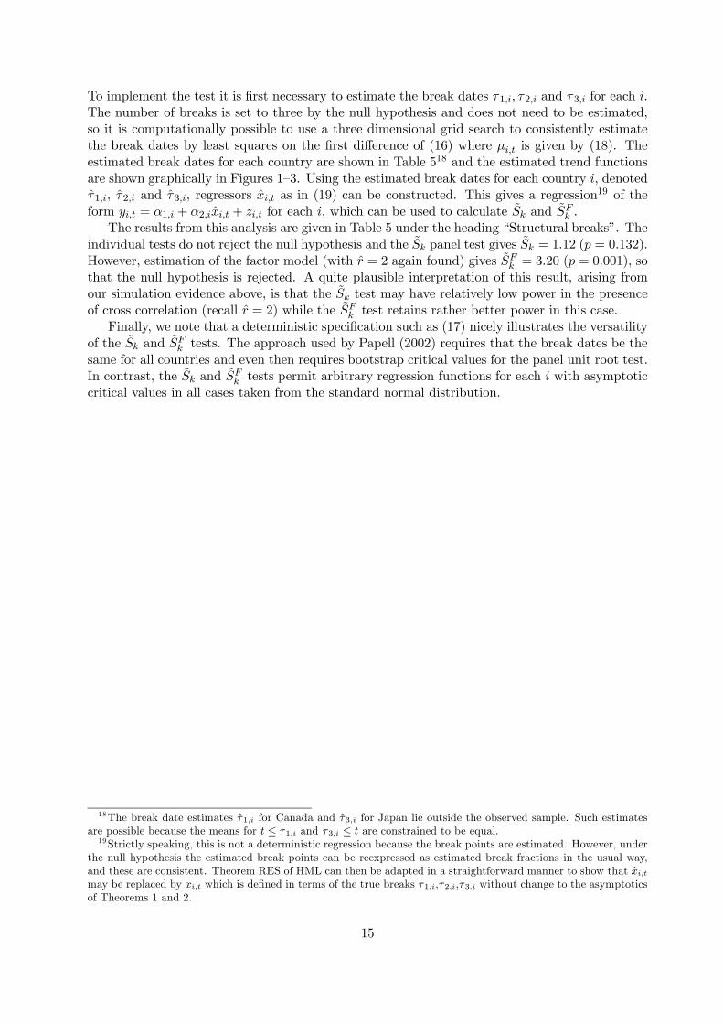
To implement the test it is first necessary to estimate the break dates τ1,i, τ2,i and τ3,i for each i.The number of breaks is set to three by the null hypothesis and does not need to be estimated,so it is computationally possible to use a three dimensional grid search to consistently estimatethe break dates by least squares on the first difference of (16) where µi,t is given by (18). Theestimated break dates for each country are shown in Table 518 and the estimated trend functionsare shown graphically in Figures 1—3. Using the estimated break dates for each country i, denotedτ1,i, τ2,i and τ3,i, regressors xi,t as in (19) can be constructed. This gives a regression19 of theform yi,t = α1,i + α2,ixi,t + zi,t for each i, which can be used to calculate Sk and SF

k .The results from this analysis are given in Table 5 under the heading “Structural breaks”. The

individual tests do not reject the null hypothesis and the Sk panel test gives Sk = 1.12 (p = 0.132).However, estimation of the factor model (with r = 2 again found) gives SF

k = 3.20 (p = 0.001), sothat the null hypothesis is rejected. A quite plausible interpretation of this result, arising fromour simulation evidence above, is that the Sk test may have relatively low power in the presenceof cross correlation (recall r = 2) while the SF

k test retains rather better power in this case.Finally, we note that a deterministic specification such as (17) nicely illustrates the versatility

of the Sk and SFk tests. The approach used by Papell (2002) requires that the break dates be the

same for all countries and even then requires bootstrap critical values for the panel unit root test.In contrast, the Sk and SF

k tests permit arbitrary regression functions for each i with asymptoticcritical values in all cases taken from the standard normal distribution.

18The break date estimates τ1,i for Canada and τ3,i for Japan lie outside the observed sample. Such estimatesare possible because the means for t ≤ τ1,i and τ3,i ≤ t are constrained to be equal.19Strictly speaking, this is not a deterministic regression because the break points are estimated. However, under

the null hypothesis the estimated break points can be reexpressed as estimated break fractions in the usual way,and these are consistent. Theorem RES of HML can then be adapted in a straightforward manner to show that xi,tmay be replaced by xi,t which is defined in terms of the true breaks τ1,i,τ2,i,τ3.i without change to the asymptoticsof Theorems 1 and 2.

15

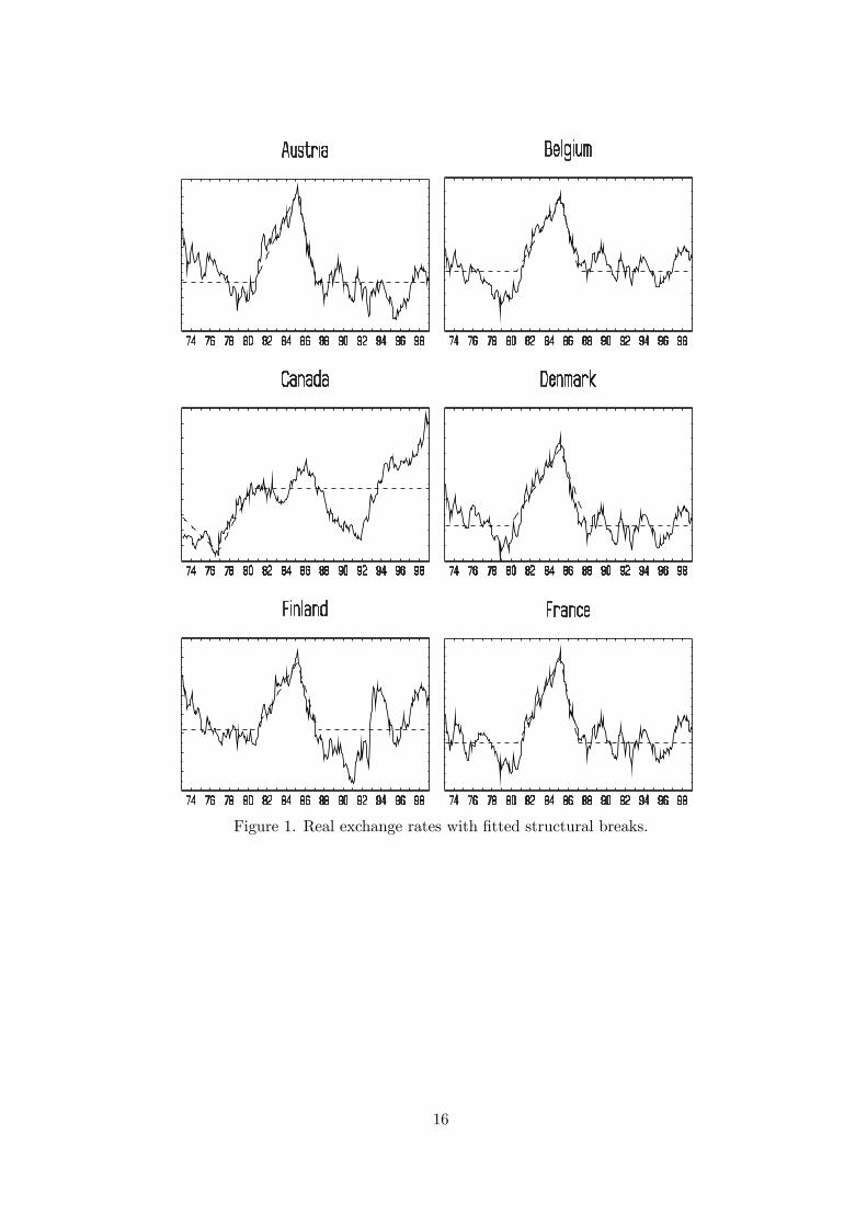
Figure 1. Real exchange rates with fitted structural breaks.

16

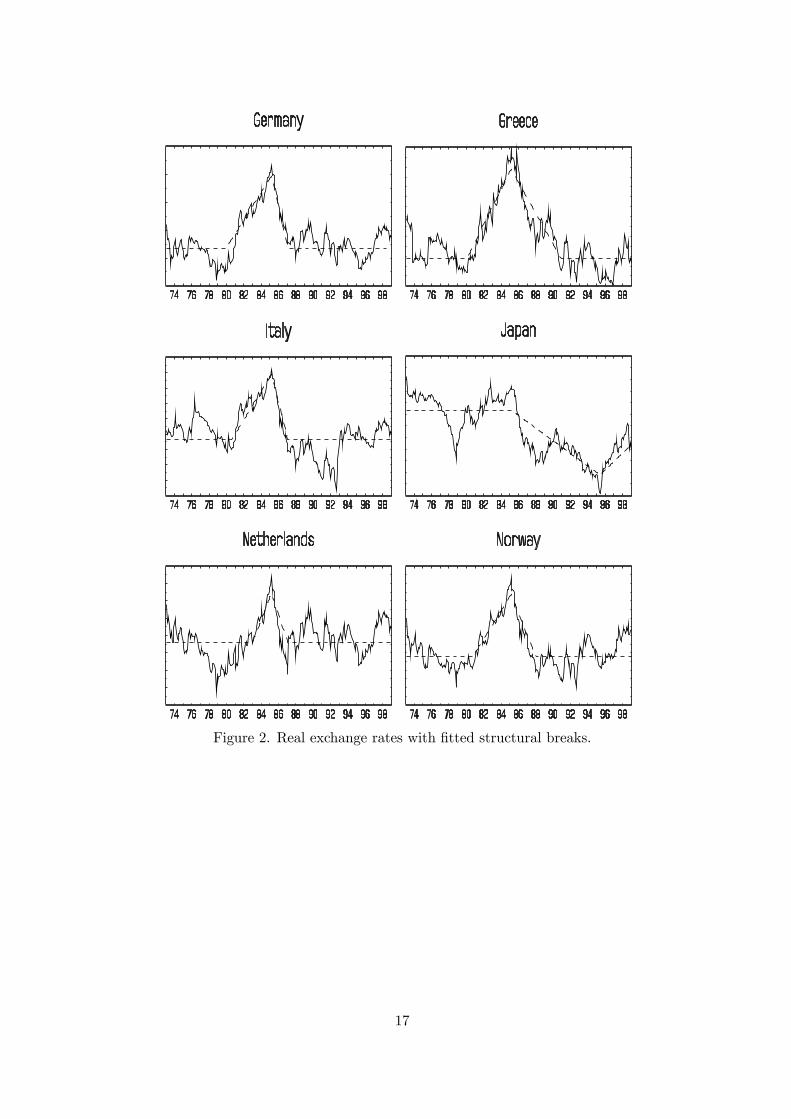
Figure 2. Real exchange rates with fitted structural breaks.

17

Figure 3. Real exchange rates with fitted structural breaks.

18

REFERENCES

Andrews, D.W.K., 1991. Heteroskedasticity and autocorrelation consistent covariance matrixestimation, Econometrica, 59, 817—858.

Bai, J. and S. Ng, 2002. Determining the number of factors in approximate factor models.Econometrica 70, 191—221.

Bai, J. and S. Ng, 2004a. A PANIC attach on unit roots and cointegration. Econometrica 72,1127—1177.

Bai, J. and S. Ng, 2004b. A new look at panel testing of stationarity and the PPP hypothesis. InIdentification and Inference in Econometric Models: Essays in Honor of Thomas J. Rothenberg,Andrews, D. and J.H. Stock (eds) Cambridge University Press.

Bai, J. and P. Perron, 1998. Estimating and testing linear models with multiple structural changes.Econometrica 66, 47—78.

Chang, Y., 2003. Bootstrap unit root tests in panels with cross-sectional dependency. Forthcom-ing, Journal of Econometrics.

Chang, Y. and Song, W., 2002. Panel unit root tests in the presence of cross-sectional dependencyand heterogeneity. Mimeo., Rice University.

Cheung, Y.W. and Lai, K., 2000. On cross-country differences in the persistence of real exchangerates. Journal of International Economics, 50, 375-397.

Choi, I., 2001. Unit root tests for panel data. Journal of International, Money and Finance, 20,219-247.

Choi, I., 2002. Combination unit root tests for cross-sectionally correlated panels. Mimeo., HongKong University.

Driscoll, J.C. and Kraay, A.C., 1998, Consistent Covariance Estimation with Spatially DependentPanel Data, Review of Economics and Statistics, 80, 549-560.

Hadri, K., 2000. Testing for stationarity in heterogeneous panel data. Econometrics Journal, 3,148-161.

Harris, D., McCabe, B.P.M. and Leybourne, S.J., 2003. Some limit theory for infinite orderautocovariances. Econometric Theory, 19, 829-864.

Kwiatkowski, D., P.C.B. Phillips, P. Schmidt and Y. Shin, 1992. Testing the null hypothesis ofstationarity against the alternative of a unit root. Journal of Econometrics 54, 159—178.

Im, K.S., Pesaran, M.H. and Shin Y., 2003. Testing for unit roots in heterogeneous panels.Journal of Econometrics, 115, 53-74.

Levin A., Lin C.F. and Chu C.S., 2002. Unit root tests in panel data: Asymptotic and finitesample properties. Journal of Econometrics, 108, 1-24.

Maddala, G.S. and Wu, S., 1999. A comparative study of unit root tests with panel data and anew simple approach. Oxford Bulletin of Economics and Statistics, 61, 631-652.

O’Connell P.G.J., 1998. The overvaluation of purchasing power parity. Journal of InternationalEconomics, 44, 1-19.

Oh., K.Y., 1996. Purchasing power parity and unit root tests using panel data. Journal ofInternational, Money and Finance, 15, 405-418.

Papell, D.H., 1997. Searching for stationarity: Purchasing power parity under the current float.Journal of International Economics, 43, 313-332.

Papell, D.H., 2002. The Great Appreciation, the Great Depreciation and the Purchasing PowerParity Hypothesis. Journal of International Economics 57, 51—82.

Shin, Y. and A. Snell (2002) Mean Group Tests for Stationarity in Heterogeneous Panels. Man-uscript, University of Edinburgh.

Wu, Y., 1996. Are real exchange rates nonstationary? Evidence from a panel-data test. Journalof Money, Credit and Banking, 28, 54-63.

19

Wu, S. and Wu, J.L., 2001. Is purchasing power parity overvalued ? Journal of Money, Creditand Banking, 33, 804-812.

Yin, Y. and S. Wu, 2000. Stationarity tests in heterogeneous panels. In Nonstationary Panels,Panel Cointegration and Dynamic Panels, Baltagi, B. (ed.) Elsevier Science.

6 Appendix

6.1 Proof of Theorem 1.

(i) Let zt = (z1,t, ..., zN,t)0 and zt = (z1,t, ..., zN,t)

0. Then Ck can be written

Ck = d0 vec

"T−1/2

TXt=k+1

ztz0t−k

#

for a selector vector d defined as d = vec[IN2 ]. Now,

vec

"T−1/2

TXt=k+1

ztz0t−k

#= vec

"T−1/2G−10

TXt=k+1

ztz0t−kG

−10

#

= (G−10 ⊗ G−10 ) vec"T−1/2

TXt=k+1

ztz0t−k

#

where G0 = diag[γ0z1,t1/2, ..., γ0zN,t1/2]. It follows from HML, Theorem 8, that

vec

"T−1/2

TXt=k+1

ztz0t−k

#⇒ N [0,Ω]

on noting that ηt = diag[(1−φ1L)−1, .., (1−φNL)−1]εt also satisfies the conditions of AssumptionLP of HML. Moreover, since G0

p→G0 = diag[E(ηtη0t)1/2],

Ck ⇒ N [0,d0(G−10 ⊗G−10 )Ω(G−10 ⊗G−10 )d]

by the continuous mapping theorem (CMT). Next, with at =PN

i=1 zi,tzi,t−k and bt = vec[ztz0t−k]

and ct = vec[ztz0t−k], we may write

ωat2 = d0Ωbtd = d0(G−10 ⊗ G−10 )Ωct(G−10 ⊗ G−10 )d

where Ω. is given in (7). From HML, Theorem 8, for a specified matrix Ω, Ωctp→ Ω and

hence, by the CMT,ωat2

p→ d0(G−10 ⊗G−10 )Ω(G−10 ⊗G−10 )dso that

Ck

ωat⇒ N [0, 1]. (20)

To deal with the bias correction c, the expectation of the estimation error under H0 using thestandardized residuals zi,t can be written

ci = trE

⎡⎣ 1s2i

ÃT−1/2

TXt=1

xi,tzi,t

!ÃT−1/2

TXt=1

xi,tzi,t

!0⎤⎦20

where xi,t =³T−1

PTt=1 xi,tx

0i,t

´−1/2xi,t. In this form ci is clearly O (1) and moreover by Theorem

1 of Andrews (1991) ci is consistently estimated by ci. Thus Sk = ωat−1³Ck +

PNi=1 T

−1/2ci´=

ωat−1Ck +Op

¡T−1/2

¢⇒ N [0, 1] from (20).

(ii) Suppose, without loss of generality, that φi = 1 for i = 1, ..., sN, 0 < s ≤ 1 and φi < 1 fori = sN + 1, ...,N (with the obvious modification for s = 1). Now

T−1/2Ck =sNXi=1

T−1TX

t=k+1

zi,tzi,t−k +NX

i=sN+1

T−1TX

t=k+1

zi,tzi,t−k,

and the second term is Op

¡T−1/2

¢from the proof of Theorem 1. Noting that T−1γ0zi,t = Op (1)

for i = 1, . . . ,M , the first term satisfies

sNXi=1

T−1TX

t=k+1

zi,tzi,t−k =sNXi=1

1

T−1γ0zitT−2

TXt=k+1

zi,tzi,t−k

=sNXi=1

1

T−1γ0zi,tT−2

TXt=1

z2i,t + op (1)

= sN + op (1) .

Thus,Ck = T 1/2sN + op

³T 1/2

´. (21)

Next, with at =PN

i=1 zi,tzi,t−k,

l−1ωat2 = l−1

⎛⎝γ0at+ 2lX

j=1

µ1− j

l

¶γjat

⎞⎠ ≤ 3γ0at (22)

where γ0at = T−1PT

t=k+1

³PNi=1 zi,tzi,t−k

´2.Thus

γ0at ≤NXi=1

NXj=1

T−1TXt=1

z2i,tz2j,t = Op (1) (23)

since for i, j = sN + 1, . . . , N ,

T−1TX

t=k+1

z2i,tz2j,t =

1

γ0zi,t.γ0zj,tT−1

TXt=k+1

z2i,tz2j,t = Op (1)

for i, j = 1, . . . , sN ,

T−1TX

t=k+1

z2i,tz2j,t =

1

T−1γ0zi,t.T−1γ0zj,tT−3

TXt=k+1

z2i,tz2j,t = Op (1)

and for i = sN + 1, . . . , N and j = 1, . . . , sN,

T−1TX

t=k+1

z2i,tz2j,t =

1

γ0zi,t.T−1γ0zj,tT−2

TXt=k+1

z2i,tz2j,t = Op (1) .

21

(and similarly for j = sN + 1, . . . , N and i = 1, . . . , sN). Combining (21), (22) and (23) we findfor any critical value c, as T →∞,

P

"Ck

ωat> c

#= P

"sN + op(1)

lT 1/2

Op(1)> c

#→ 1

since l = o(T 1/2). The bias correction c obviously does not affect test consistency since eachT−1/2ci is non-negative.

6.2 Deterministic Regressions in the Factor Model

In standard notation, the model (14) (where xi,t is an mi× 1 vector of regressors) can be written

y(NT×1)

= X(NT×m)

β(m×1)

+ z(NT×1)

, (24)

where y = (y01, . . . ,y0N )

0, X = diag (X1, . . . ,XN), β =¡β01, . . . ,β

0N

¢0, z = (z01, . . . , z0N)

0, m =PNi=1mi and yi = (yi,1, . . . , yi,T )

0, Xi = (xi,1, . . . ,xi,T )0, zi = (zi,1, . . . , zi,T )

0. The factor model(10) can be written

Z(T×N)

= F(T×r)

Λ(r×N)

+ E(T×N)

(25)

where Z = (z1, . . . , zN), F = (f1, . . . , fr)0, Λ = (λ1, . . . ,λN ) and E = (e1, . . . , eN ) where ei =

(ei,1, . . . , ei,T )0 for each i = 1, . . . , N .

The estimation of the factor model in first differences proceeds as follows. The first differenceof equation (24) can be written

∆y(N(T−1)×1)

= (∆XC)(N(T−1)×m∆)

βC(m∆×1)

+ ∆z(N(T−1)×1)

,

where βC = (C0C)−1C0β and C is an m×m∆ matrix chosen to exclude columns of ∆X corre-

sponding to constant terms in X so that ∆XC has full column rank m∆ ≤ m. The residuals fromthis regression can be written c∆z = ∆y− (∆XC) βC , where βC = (C

0∆X0∆XC)−1C0∆X0∆y is

the usual OLS estimator, and the (T − 1) ×N matrix d∆Z is defined to satisfy c∆z = vec³d∆Z´.The estimated factors can then be writtend∆F =d∆ZΓ where Γ is the N×r matrix of eigenvectorscorresponding to the largest r eigenvalues of d∆Z0d∆Z. The estimated idiosyncratic componentsare thend∆E =d∆Z−d∆FΛ where Λ = ³d∆F0d∆F´−1d∆F0d∆Z. Taking the partial sums ofd∆F andd∆E gives the component estimates F and E, with corresponding r (T − 1)× 1 and N (T − 1)× 1vectors f = vec

³F´and e = vec

³E´.

The deterministic regressions for the estimated factors f proceed as follows. Since f canbe written f =

³Γ0 ⊗ IT−1

´ c∆z, it is necessary to regress f on ³Γ0 ⊗ IT−1´X. However thisregressor matrix may not have full column rank, in which case it is sufficient to regress f onXf =

³Γ0 ⊗ IT−1

´XCf where Cf is a matrix chosen such that Xf has full column rank and its

columns form a basis for the vector space containing the columns of³Γ0 ⊗ IT−1

´X. In practice,

if³Γ0 ⊗ IT−1

´X has less than full column rank, a simple choice for Cf is the matrix of eigen-

vectors corresponding to the non-zero eigenvalues of X0³ΓΓ

0 ⊗ IT−1´X. The residuals from the

regression of f on Xf are denotedbf . The corresponding (T − 1)× r matrix bF is defined to satisfy

22

bf = vec

³bF´. Each of the r columns of bF is standardized by its sample standard deviation to give

the (T − 1)×r matrix F, whose individual elements are denoted fj,t, j = 1, . . . , r and t = 2, . . . , T .The deterministic regressions for the estimated idiosyncratic components e proceed similarly.

We can write d∆E = d∆Z −d∆Z³ΓΛ´ since d∆F = d∆ZΓ, so e = ³IN(T−1) −

³Λ0Γ0 ⊗ IT−1

´´z .

Therefore it is necessary to regress e on³IN(T−1) −

³Λ0Γ0 ⊗ IT−1

´´X. If this regressor matrix

does not have full rank then it is replaced by Xe =³IN(T−1) −

³Λ0Γ0 ⊗ IT−1

´´XCe where, like

Cf , Ce is chosen (by principal components or other means) so that the columns of Xe provide a

basis for those of³IN(T−1) −

³Λ0Γ0 ⊗ IT−1

´´X. The residuals from the regression of e on Xe are

denoted be and the columns of the corresponding matrix bE (i.e. be = vec³bE´) and standardizedby their respective standard deviations to give E with individual elements ei,t.

To calculate the statistic (8), define ak,t =Pr

j=1 fj,tfj,t−k +PN

i=1 ei,tei,t−k. Then Ck andω ak,t are calculated as described following equation (8). The bias correction term c in (8) isgiven by

c = (T − k)−1/2 trh¡X0fXf/T

¢−1Ω wf,s+

¡X0eXe/T

¢−1Ω we,s

i,

where wf = Xf ¯ fι0mf

=nw0f,s

or(T−1)s=1

and we = Xe ¯ eι0me=©w0e,s

ªN(T−1)s=1

, where ¯ is the

Hadamard product, ιm is an m× 1 vector of ones, mf and me are the column dimensions of Xf

and Xe respectively.

6.3 Proof of Theorem 2

In the notation defined in Section 6.2, the residuals c∆z can be writtenc∆z = ∆z−∆XC ¡C0∆X0∆XC¢−1C0∆X0∆z.

Taking partial sums of c∆z givesz = z−XC

¡C0∆X0∆XC

¢−1C0∆X0∆z

apart from some asymptotically negligible initial value effects, so that z andX now haveN (T − 1)rows.

The partial sum of c∆f = vec³d∆F´ = ³Γ0 ⊗ IT−1´ c∆z givesf =

³Γ0 ⊗ IT−1

´z−XfBf

where Xf =³Γ0 ⊗ IT−1

´XCf and Bf =

³C0fCf

´−1C0fC (C

0∆X0∆XC)−1C0∆X0∆z. Thus

regressing f on Xf will remove the XfBf term from the residuals, giving

bf = Pf f = Pf

³Γ0 ⊗ IT−1

´z, (26)

where Pf = Ir(T−1) −Xf

³X0fXf

´−1X0f = Ir(T−1) − Pf . The corresponding matrix

bF satisfiesb

f = vec³bF´ and the standardized matrix F is found by F = bFG−1f , where Gf is an r×r diagonal

matrix containing the sample standard deviations of the columns of bF on the diagonal. Thus

f =³G−1f ⊗ IT−1

´bf .

23

The partial sum of c∆e = Ac∆z where A = IN(T−1) −³Λ0Γ0 ⊗ IT−1

´gives

e = Az−XeBe

whereXe =³IN(T−1) −

³Λ0Γ0⊗IT−1

´´XCe andBe = (C

0eCe)

−1C0eC (C0∆X0∆XC)−1C0∆X0∆z

so regressing e on Xe will remove Xe. This leavesbe = Pee = PeAz (27)

where Pe is the orthogonal projection on Xe. The corresponding matrixbE satisfies be = vec³bE´

and the standardized matrix E is found by E =bEG−1e , where Ge is an r × r diagonal matrix

containing the sample standard deviations of the columns of bE on the diagonal. These stepsshow that the appropriate regressions of f on Xf and e on Xe remove the effects of the initialdeterministic regression in first differences.

Since the model is estimated in differences, it follows that under both null and alternatived∆Z0d∆Z/T = Σ∆∆+Op

¡T−1/2

¢and hence Γ = Γ+Op

¡T−1/2

¢where Γ is the matrix of eigenvec-

tors corresponding to the largest r eigenvalues of Σ∆∆. Thus Λ =³Γ0d∆Z0d∆ZΓ´−1 Γ0d∆Z0d∆Z =

(Γ0Σ∆∆Γ)−1ΓΣ∆∆+Op

¡T−1/2

¢. Recalling the definitions of bf and be in (26) and (27) respectively,

consider f =³Γ0⊗IT−1

´z and e = Az. We can write

¡f 0, e0

¢0= vec

³WC

´whereW = ZΣ

−1/2∆∆

and C = Σ1/2∆∆

³Γ, P

´where P = IN−ΓΛ and Σ∆∆= E (∆zt∆z

0t). Now C = C + Op

¡T−1/2

¢where C = Σ

1/2∆∆ (Γ,P) and P = IN−Γ (Γ0Σ∆∆Γ)

−1ΓΣ∆∆. Note that C has rank N since (i)Γ has full column rank r, (ii) P has rank20 N − r and (iii) Γ0Σ∆∆P = 0. This shows that¡f 0, e0

¢0= vec

³WC

´is, even asymptotically, a rank N linear transformation of Z and hence that

all series of¡f 0, e0

¢0 are I (0) if all series of Z are I (0) and also that¡f 0, e0

¢0 must contain I (1)

elements if Z does. Therefore Theorem 1 can be applied to¡f 0, e0

¢0. The effect of the detrendingregressions represented by the projections Pf and Pe can be handled as in Theorem RES of HML.The preceding arguments hold for every r = 0, 1, . . . , rmax and hence hold when r is replaced byr ∈ 0, 1, . . . , rmax.

20P 0 = Σ1/2∆∆P

∗Σ−1/2∆∆ where P ∗ = IN − Σ

1/2∆∆Γ (Γ

0Σ∆∆Γ)−1

Γ0Σ1/2∆∆ is idempotent with trP ∗ = N − r and hence

has rank N − r.

24

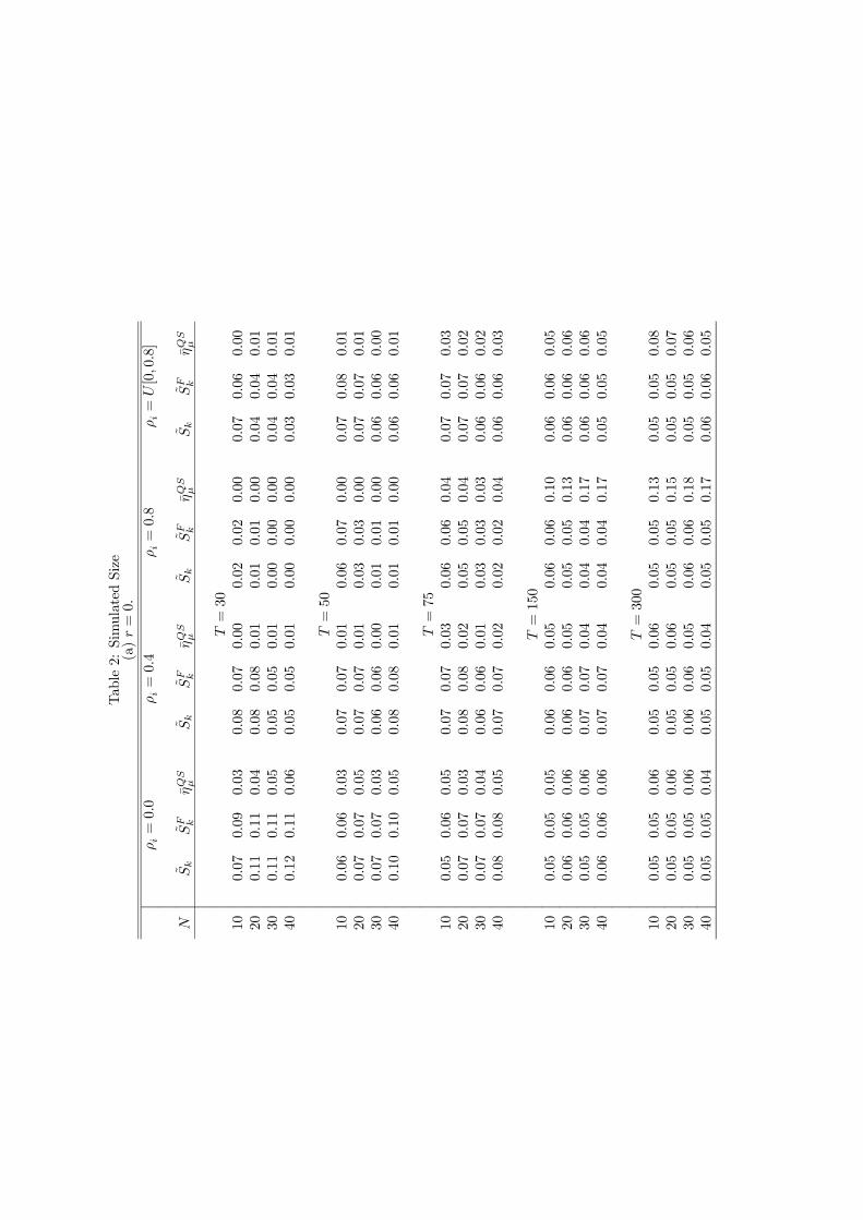
Table2:SimulatedSize

(a)r=0.

ρi=0.0

ρi=0.4

ρi=0.8

ρi=U[0,0.8]

NSk

SF k

ηQS

µSk

SF k

ηQS

µSk

SF k

ηQS

µSk

SF k

ηQS

µ

T=30

100.07

0.09

0.03

0.08

0.07

0.00

0.02

0.02

0.00

0.07

0.06

0.00

200.11

0.11

0.04

0.08

0.08

0.01

0.01

0.01

0.00

0.04

0.04

0.01

300.11

0.11

0.05

0.05

0.05

0.01

0.00

0.00

0.00

0.04

0.04

0.01

400.12

0.11

0.06

0.05

0.05

0.01

0.00

0.00

0.00

0.03

0.03

0.01

T=50

100.06

0.06

0.03

0.07

0.07

0.01

0.06

0.07

0.00

0.07

0.08

0.01

200.07

0.07

0.05

0.07

0.07

0.01

0.03

0.03

0.00

0.07

0.07

0.01

300.07

0.07

0.03

0.06

0.06

0.00

0.01

0.01

0.00

0.06

0.06

0.00

400.10

0.10

0.05

0.08

0.08

0.01

0.01

0.01

0.00

0.06

0.06

0.01

T=75

100.05

0.06

0.05

0.07

0.07

0.03

0.06

0.06

0.04

0.07

0.07

0.03

200.07

0.07

0.03

0.08

0.08

0.02

0.05

0.05

0.04

0.07

0.07

0.02

300.07

0.07

0.04

0.06

0.06

0.01

0.03

0.03

0.03

0.06

0.06

0.02

400.08

0.08

0.05

0.07

0.07

0.02

0.02

0.02

0.04

0.06

0.06

0.03

T=150

100.05

0.05

0.05

0.06

0.06

0.05

0.06

0.06

0.10

0.06

0.06

0.05

200.06

0.06

0.06

0.06

0.06

0.05

0.05

0.05

0.13

0.06

0.06

0.06

300.05

0.05

0.06

0.07

0.07

0.04

0.04

0.04

0.17

0.06

0.06

0.06

400.06

0.06

0.06

0.07

0.07

0.04

0.04

0.04

0.17

0.05

0.05

0.05

T=300

100.05

0.05

0.06

0.05

0.05

0.06

0.05

0.05

0.13

0.05

0.05

0.08

200.05

0.05

0.06

0.05

0.05

0.06

0.05

0.05

0.15

0.05

0.05

0.07

300.05

0.05

0.06

0.06

0.06

0.05

0.06

0.06

0.18

0.05

0.05

0.06

400.05

0.05

0.04

0.05

0.05

0.04

0.05

0.05

0.17

0.06

0.06

0.05

(b)r=2.

αj=0.0

ρi=0.0

αj=0.4

ρi=0.0

αj=0.8

ρi=0.0

αj=0.0

ρi=0.4

αj=0.0

ρi=0.8

αj=U[0,0.8]

ρi=U[0,0.8]

NSk

SF k

ηQS

µSk

SF k

ηQS

µSk

SF k

ηQS

µSk

SF k

ηQS

µSk

SF k

ηQS

µSk

SF k

ηQS

µ

T=30

100.03

0.08

0.03

0.05

0.10

0.02

0.07

0.07

0.01

0.04

0.08

0.01

0.06

0.03

0.00

0.06

0.06

0.00

200.03

0.10

0.02

0.05

0.10

0.02

0.08

0.07

0.01

0.03

0.07

0.01

0.06

0.01

0.00

0.06

0.05

0.00

300.03

0.11

0.03

0.05

0.09

0.02

0.07

0.07

0.01

0.04

0.05

0.01

0.04

0.00

0.00

0.06

0.02

0.00

400.02

0.11

0.03

0.05

0.10

0.02

0.06

0.07

0.01

0.04

0.05

0.00

0.06

0.00

0.00

0.07

0.03

0.00

T=50

100.03

0.07

0.04

0.05

0.07

0.03

0.08

0.07

0.05

0.04

0.07

0.01

0.05

0.06

0.01

0.05

0.06

0.00

200.04

0.09

0.02

0.05

0.09

0.02

0.07

0.09

0.06

0.04

0.08

0.01

0.06

0.02

0.00

0.06

0.07

0.00

300.04

0.09

0.01

0.06

0.09

0.02

0.09

0.09

0.05

0.05

0.07

0.00

0.05

0.02

0.00

0.07

0.06

0.00

400.03

0.09

0.02

0.05

0.09

0.02

0.08

0.09

0.07

0.03

0.07

0.00

0.06

0.01

0.00

0.05

0.06

0.00

T=75

100.05

0.06

0.05

0.05

0.06

0.05

0.07

0.06

0.08

0.04

0.06

0.03

0.05

0.07

0.06

0.05

0.06

0.04

200.05

0.07

0.03

0.06

0.07

0.04

0.07

0.08

0.11

0.05

0.08

0.01

0.06

0.05

0.03

0.06

0.07

0.01

300.05

0.07

0.03

0.05

0.06

0.04

0.07

0.08

0.12

0.04

0.08

0.01

0.05

0.04

0.03

0.05

0.07

0.02

400.04

0.09

0.03

0.06

0.08

0.05

0.07

0.08

0.16

0.05

0.09

0.01

0.05

0.02

0.02

0.06

0.06

0.03

T=150

100.05

0.05

0.06

0.06

0.04

0.08

0.06

0.05

0.11

0.04

0.06

0.06

0.04

0.07

0.09

0.05

0.06

0.08

200.05

0.06

0.05

0.06

0.06

0.05

0.06

0.05

0.14

0.05

0.06

0.04

0.05

0.04

0.11

0.05

0.07

0.05

300.04

0.06

0.05

0.05

0.05

0.06

0.06

0.06

0.17

0.04

0.05

0.04

0.05

0.04

0.13

0.06

0.06

0.07

400.04

0.05

0.05

0.06

0.07

0.05

0.06

0.07

0.18

0.04

0.06

0.04

0.04

0.04

0.14

0.05

0.05

0.05

T=300

100.04

0.05

0.07

0.05

0.04

0.06

0.06

0.05

0.12

0.05

0.05

0.06

0.04

0.06

0.11

0.06

0.05

0.08

200.04

0.05

0.05

0.05

0.05

0.06

0.06

0.05

0.13

0.05

0.05

0.05

0.05

0.06

0.15

0.05

0.05

0.09

300.05

0.05

0.05

0.05

0.05

0.06

0.06

0.05

0.12

0.05

0.05

0.04

0.05

0.05

0.16

0.06

0.05

0.07

400.05

0.05

0.04

0.05

0.06

0.04

0.06

0.06

0.12

0.04

0.05

0.04

0.05

0.06

0.16

0.06

0.06

0.06

(c)r=7.

αj=0.0

ρi=0.0

αj=0.4

ρi=0.0

αj=0.8

ρi=0.0

αj=0.0

ρi=0.4

αj=0.0

ρi=0.8

αj=U[0,0.8]

ρi=U[0,0.8]

NSk

SF k

ηQS

µSk

SF k

ηQS

µSk

SF k

ηQS

µSk

SF k

ηQS

µSk

SF k

ηQS

µSk

SF k

ηQS

µ

T=30

100.03

0.08

0.03

0.06

0.08

0.01

0.07

0.04

0.00

0.03

0.09

0.01

0.04

0.07

0.01

0.05

0.07

0.01

200.04

0.09

0.03

0.07

0.08

0.01

0.07

0.06

0.00

0.04

0.09

0.01

0.04

0.06

0.00

0.07

0.06

0.00

300.04

0.07

0.06

0.08

0.08

0.02

0.07

0.09

0.00

0.05

0.08

0.03

0.04

0.08

0.00

0.07

0.08

0.01

400.04

0.06

0.07

0.08

0.08

0.02

0.05

0.07

0.00

0.04

0.09

0.02

0.04

0.08

0.00

0.07

0.07

0.00

T=50

100.03

0.06

0.06

0.06

0.07

0.04

0.09

0.08

0.04

0.04

0.07

0.03

0.04

0.08

0.02

0.06

0.07

0.03

200.04

0.05

0.12

0.04

0.07

0.10

0.07

0.08

0.12

0.04

0.07

0.05

0.05

0.08

0.00

0.06

0.07

0.05

300.04

0.05

0.15

0.06

0.06

0.15

0.07

0.10

0.17

0.04

0.07

0.09

0.04

0.07

0.01

0.07

0.07

0.12

400.04

0.06

0.20

0.06

0.06

0.16

0.08

0.09

0.19

0.04

0.06

0.11

0.04

0.08

0.01

0.06

0.08

0.15

T=75

100.05

0.05

0.07

0.06

0.06

0.08

0.07

0.07

0.12

0.04

0.07

0.05

0.05

0.08

0.05

0.06

0.06

0.09

200.05

0.05

0.15

0.06

0.06

0.17

0.06

0.08

0.25

0.05

0.06

0.12

0.05

0.07

0.05

0.06

0.07

0.15

300.05

0.04

0.17

0.06

0.07

0.19

0.08

0.07

0.26

0.05

0.05

0.10

0.05

0.07

0.05

0.05

0.06

0.19

400.05

0.05

0.24

0.05

0.06

0.22

0.07

0.09

0.32

0.05

0.05

0.18

0.05

0.07

0.09

0.06

0.06

0.20

T=150

100.04

0.06

0.07

0.04

0.06

0.09

0.06

0.06

0.19

0.05

0.06

0.06

0.05

0.06

0.09

0.06

0.06

0.09

200.05

0.05

0.17

0.05

0.05

0.19

0.06

0.07

0.27

0.05

0.05

0.15

0.05

0.04

0.11

0.06

0.05

0.20

300.05

0.06

0.19

0.04

0.06

0.24

0.06

0.06

0.29

0.05

0.05

0.16

0.06

0.05

0.14

0.06

0.06

0.24

400.05

0.04

0.22

0.06

0.05

0.23

0.07

0.07

0.31

0.04

0.05

0.18

0.06

0.05

0.17

0.06

0.05

0.23

T=300

100.05

0.05

0.10

0.05

0.05

0.11

0.06

0.06

0.20

0.05

0.05

0.10

0.05

0.05

0.13

0.05

0.05

0.13

200.05

0.05

0.17

0.05

0.05

0.21

0.06

0.06

0.26

0.05

0.05

0.14

0.05

0.05

0.13

0.05

0.05

0.23

300.05

0.04

0.18

0.05

0.05

0.20

0.06

0.06

0.29

0.04

0.05

0.14

0.05

0.05

0.14

0.05

0.05

0.24

400.05

0.05

0.18

0.05

0.06

0.22

0.06

0.06

0.28

0.05

0.05

0.17

0.05

0.04

0.15

0.05

0.05

0.25

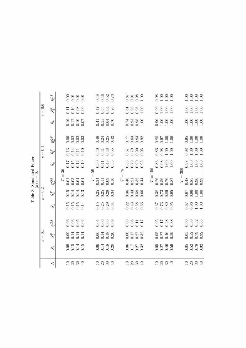
Table3:SimulatedPower

(a)r=0.

s=0.1

s=0.2

s=0.4

s=0.6

NSk

SF k

ηQS

µSk

SF k

ηQS

µSk

SF k

ηQS

µSk

SF k

ηQS

µ

T=30

100.09

0.09

0.03

0.15

0.15

0.01

0.17

0.13

0.00

0.16

0.11

0.00

200.15

0.14

0.03

0.15

0.14

0.03

0.15

0.14

0.02

0.12

0.10

0.01

300.14

0.14

0.05

0.15

0.14

0.04

0.12

0.11

0.02

0.10

0.08

0.01

400.15

0.14

0.04

0.14

0.13

0.04

0.10

0.10

0.02

0.07

0.06

0.01

T=50

100.06

0.06

0.04

0.15

0.25

0.34

0.30

0.40

0.46

0.41

0.47

0.48

200.14

0.14

0.06

0.25

0.25

0.11

0.41

0.41

0.24

0.55

0.55

0.46

300.18

0.18

0.05

0.29

0.29

0.09

0.48

0.48

0.25

0.64

0.64

0.52

400.20

0.20

0.09

0.34

0.34

0.16

0.55

0.55

0.42

0.70

0.70

0.73

T=75

100.06

0.06

0.05

0.22

0.36

0.46

0.55

0.67

0.77

0.74

0.81

0.87

200.17

0.17

0.08

0.43

0.43

0.21

0.79

0.79

0.63

0.93

0.93

0.91

300.27

0.27

0.11

0.58

0.58

0.32

0.90

0.90

0.83

0.98

0.98

0.98

400.32

0.32

0.17

0.66

0.66

0.44

0.95

0.95

0.92

1.00

1.00

1.00

T=150

100.05

0.05

0.05

0.37

0.38

0.26

0.83

0.86

0.88

0.96

0.96

0.98

200.27

0.27

0.17

0.73

0.73

0.56

0.98

0.98

0.97

1.00

1.00

1.00

300.46

0.46

0.28

0.89

0.89

0.76

1.00

1.00

1.00

1.00

1.00

1.00

400.59

0.59

0.38

0.95

0.95

0.87

1.00

1.00

1.00

1.00

1.00

1.00

T=300

100.05

0.05

0.06

0.67

0.67

0.48

0.98

0.98

0.95

1.00

1.00

1.00

200.52

0.52

0.30

0.96

0.96

0.85

1.00

1.00

1.00

1.00

1.00

1.00

300.79

0.79

0.52

1.00

1.00

0.96

1.00

1.00

1.00

1.00

1.00

1.00

400.92

0.92

0.65

1.00

1.00

0.99

1.00

1.00

1.00

1.00

1.00

1.00

(b)r=2.

s=0.1

αj=0

s=0.2

αj=0

s=0.4

αj=0

s=0.6

αj=0

s=0

αj=1

NSk

SF k

ηQS

µSk

SF k

ηQS

µSk

SF k

ηQS

µSk

SF k

ηQS

µSk

SF k

ηQS

µ

T=30

100.02

0.10

0.03

0.02

0.14

0.01

0.05

0.14

0.00

0.08

0.11

0.00

0.19

0.14

0.00

200.03

0.14

0.01

0.04

0.13

0.01

0.08

0.10

0.00

0.09

0.07

0.00

0.18

0.13

0.00

300.03

0.14

0.02

0.04

0.11

0.01

0.05

0.07

0.01

0.07

0.05

0.00

0.19

0.14

0.00

400.03

0.13

0.02

0.04

0.11

0.01

0.04

0.06

0.00

0.08

0.03

0.00

0.18

0.14

0.01

T=50

100.04

0.07

0.03

0.05

0.27

0.32

0.08

0.41

0.42

0.11

0.48

0.43

0.38

0.35

0.43

200.03

0.21

0.23

0.05

0.34

0.36

0.05

0.49

0.52

0.07

0.57

0.57

0.35

0.38

0.55

300.05

0.24

0.23

0.07

0.36

0.32

0.11

0.52

0.48

0.15

0.64

0.60

0.39

0.39

0.57

400.05

0.23

0.15

0.05

0.38

0.40

0.09

0.57

0.57

0.12

0.68

0.73

0.36

0.40

0.62

T=75

100.04

0.06

0.05

0.06

0.43

0.59

0.10

0.70

0.79

0.19

0.81

0.88

0.55

0.54

0.71

200.06

0.29

0.43

0.10

0.60

0.69

0.15

0.87

0.86

0.34

0.95

0.95

0.60

0.60

0.77

300.06

0.39

0.49

0.09

0.69

0.72

0.21

0.93

0.92

0.32

0.99

0.99

0.59

0.61

0.81

400.06

0.45

0.59

0.08

0.78

0.81

0.17

0.97

0.96

0.25

1.00

1.00

0.59

0.63

0.82

T=150

100.05

0.05

0.07

0.08

0.61

0.74

0.25

0.89

0.96

0.59

0.96

0.99

0.77

0.76

0.89

200.08

0.54

0.69

0.17

0.84

0.92

0.42

0.99

1.00

0.67

1.00

1.00

0.79

0.81

0.93

300.08

0.63

0.81

0.18

0.94

0.97

0.47

1.00

1.00

0.76

1.00

1.00

0.78

0.81

0.93

400.07

0.83

0.92

0.17

0.98

0.99

0.53

1.00

1.00

0.87

1.00

1.00

0.78

0.81

0.93

T=300

100.05

0.06

0.06

0.11

0.83

0.88

0.39

0.99

0.99

0.83

1.00

1.00

0.92

0.95

0.97

200.11

0.79

0.87

0.32

0.99

0.99

0.88

1.00

1.00

1.00

1.00

1.00

0.96

0.95

0.98

300.16

0.89

0.94

0.46

1.00

1.00

0.93

1.00

1.00

1.00

1.00

1.00

0.95

0.96

0.98

400.16

0.98

0.98

0.49

1.00

1.00

0.95

1.00

1.00

1.00

1.00

1.00

0.96

0.97

0.98

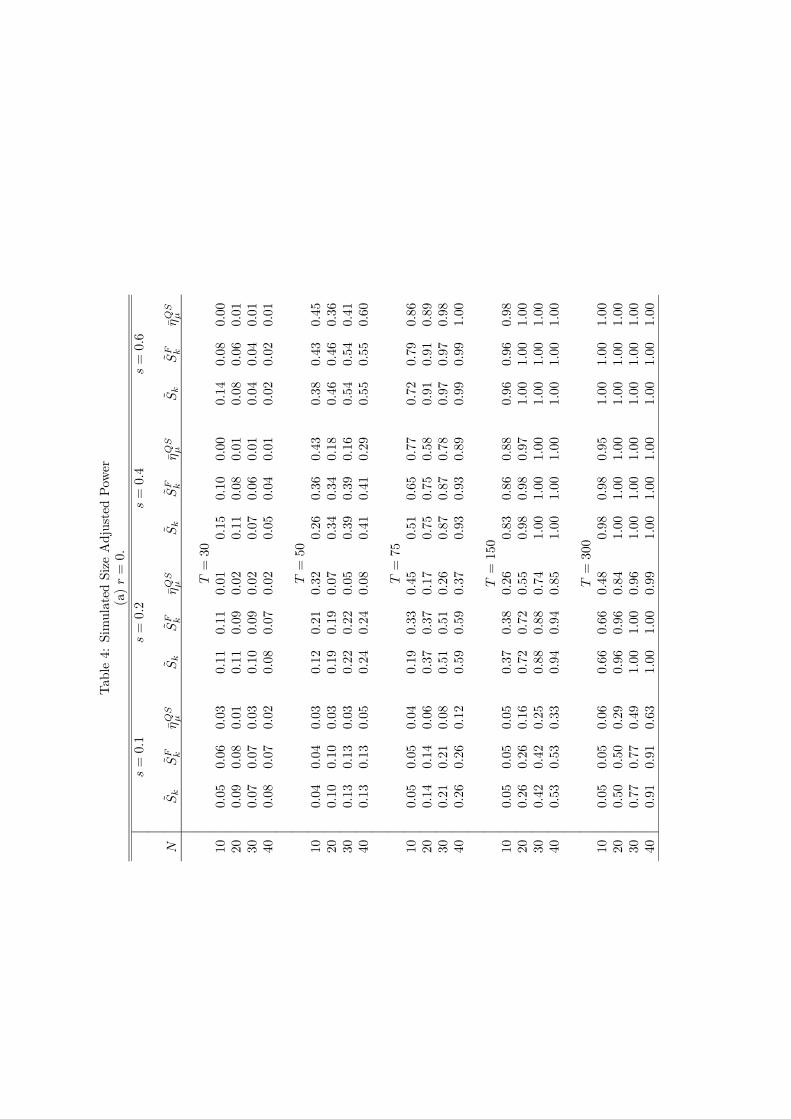
Table4:SimulatedSizeAdjustedPower

(a)r=0.

s=0.1

s=0.2

s=0.4

s=0.6

NSk

SF k

ηQS

µSk

SF k

ηQS

µSk

SF k

ηQS

µSk

SF k

ηQS

µ

T=30

100.05

0.06

0.03

0.11

0.11

0.01

0.15

0.10

0.00

0.14

0.08

0.00

200.09

0.08

0.01

0.11

0.09

0.02

0.11

0.08

0.01

0.08

0.06

0.01

300.07

0.07

0.03

0.10

0.09

0.02

0.07

0.06

0.01

0.04

0.04

0.01

400.08

0.07

0.02

0.08

0.07

0.02

0.05

0.04

0.01

0.02

0.02

0.01

T=50

100.04

0.04

0.03

0.12

0.21

0.32

0.26

0.36

0.43

0.38

0.43

0.45

200.10

0.10

0.03

0.19

0.19

0.07

0.34

0.34

0.18

0.46

0.46

0.36

300.13

0.13

0.03

0.22

0.22

0.05

0.39

0.39

0.16

0.54

0.54

0.41

400.13

0.13

0.05

0.24

0.24

0.08

0.41

0.41

0.29

0.55

0.55

0.60

T=75

100.05

0.05

0.04

0.19

0.33

0.45

0.51

0.65

0.77

0.72

0.79

0.86

200.14

0.14

0.06

0.37

0.37

0.17

0.75

0.75

0.58

0.91

0.91

0.89

300.21

0.21

0.08

0.51

0.51

0.26

0.87

0.87

0.78

0.97

0.97

0.98

400.26

0.26

0.12

0.59

0.59

0.37

0.93

0.93

0.89

0.99

0.99

1.00

T=150

100.05

0.05

0.05

0.37

0.38

0.26

0.83

0.86

0.88

0.96

0.96

0.98

200.26

0.26

0.16

0.72

0.72

0.55

0.98

0.98

0.97

1.00

1.00

1.00

300.42

0.42

0.25

0.88

0.88

0.74

1.00

1.00

1.00

1.00

1.00

1.00

400.53

0.53

0.33

0.94

0.94

0.85

1.00

1.00

1.00

1.00

1.00

1.00

T=300

100.05

0.05

0.06

0.66

0.66

0.48

0.98

0.98

0.95

1.00

1.00

1.00

200.50

0.50

0.29

0.96

0.96

0.84

1.00

1.00

1.00

1.00

1.00

1.00

300.77

0.77

0.49

1.00

1.00

0.96

1.00

1.00

1.00

1.00

1.00

1.00

400.91

0.91

0.63

1.00

1.00

0.99

1.00

1.00

1.00

1.00

1.00

1.00

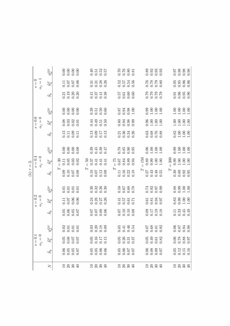
(b)r=2.

s=0.1

αj=0

s=0.2

αj=0

s=0.4

αj=0

s=0.6

αj=0

s=0

αj=1

NSk

SF k

ηQS

µSk

SF k

ηQS

µSk

SF k

ηQS

µSk

SF k

ηQS

µSk

SF k

ηQS

µ

T=30

100.06

0.05

0.02

0.05

0.11

0.01

0.09

0.11

0.00

0.13

0.08

0.00

0.21

0.11

0.00

200.05

0.08

0.01

0.06

0.07

0.01

0.10

0.05

0.00

0.11

0.03

0.00

0.19

0.07

0.00

300.05

0.07

0.01

0.05

0.06

0.01

0.07

0.03

0.00

0.09

0.02

0.00

0.20

0.07

0.00

400.07

0.07

0.01

0.07

0.06

0.01

0.08

0.02

0.00

0.11

0.01

0.00

0.20

0.06

0.00

T=50

100.05

0.05

0.03

0.07

0.24

0.30

0.10

0.37

0.39

0.13

0.44

0.39

0.41

0.31

0.40

200.05

0.16

0.20

0.07

0.28

0.32

0.07

0.41

0.45

0.09

0.49

0.51

0.37

0.31

0.51

300.06

0.17

0.18

0.08

0.27

0.26

0.12

0.41

0.39

0.17

0.51

0.50

0.41

0.28

0.52

400.06

0.15

0.09

0.06

0.26

0.30

0.09

0.41

0.47

0.13

0.50

0.60

0.38

0.26

0.57

T=75

100.05

0.05

0.05

0.07

0.41

0.58

0.11

0.67

0.78

0.21

0.80

0.87

0.57

0.52

0.70

200.06

0.26

0.41

0.10

0.57

0.67

0.16

0.84

0.85

0.36

0.94

0.94

0.61

0.57

0.76

300.07

0.31

0.46

0.10

0.61

0.68

0.22

0.89

0.90

0.34

0.98

0.98

0.60

0.54

0.80

400.07

0.37

0.54

0.08

0.71

0.78

0.18

0.94

0.95

0.26

0.99

1.00

0.60

0.56

0.81

T=150

100.06

0.05

0.07

0.09

0.61

0.74

0.27

0.89

0.96

0.63

0.96

0.99

0.79

0.76

0.89

200.08

0.49

0.68

0.17

0.81

0.92

0.43

0.99

1.00

0.68

1.00

1.00

0.79

0.78

0.92

300.09

0.61

0.81

0.19

0.94

0.97

0.48

1.00

1.00

0.76

1.00

1.00

0.79

0.79

0.93

400.07

0.82

0.92

0.18

0.97

0.99

0.55

1.00

1.00

0.88

1.00

1.00

0.79

0.80

0.93

T=300

100.05

0.06

0.06

0.11

0.83

0.88

0.39

0.99

0.99

0.82

1.00

1.00

0.91

0.95

0.97

200.12

0.78

0.87

0.33

0.99

0.99

0.89

1.00

1.00

1.00

1.00

1.00

0.96

0.95

0.98

300.15

0.88

0.94

0.45

1.00

1.00

0.92

1.00

1.00

1.00

1.00

1.00

0.95

0.96

0.98

400.16

0.97

0.98

0.49

1.00

1.00

0.95

1.00

1.00

1.00

1.00

1.00

0.96

0.96

0.98

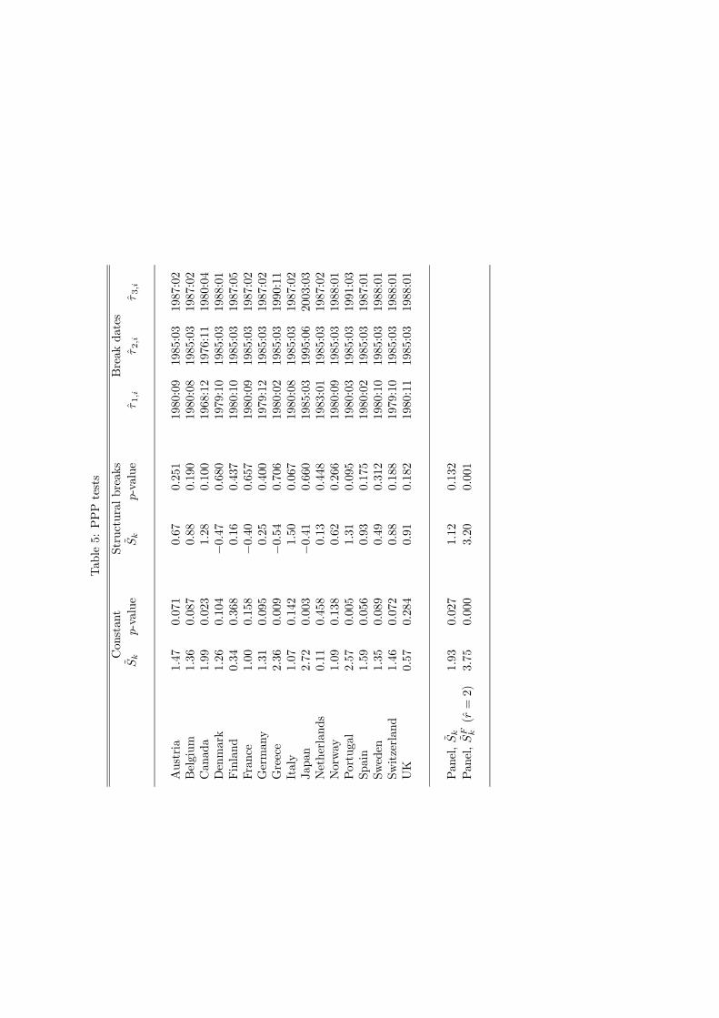
Table5:PPPtests

Constant

Structuralbreaks

Breakdates

Sk

p-value

Sk

p-value

τ1,i

τ2,i

τ3,i

Austria

1.47

0.071

0.67

0.251

1980:09

1985:03

1987:02

Belgium

1.36

0.087

0.88

0.190

1980:08

1985:03

1987:02

Canada

1.99

0.023

1.28

0.100

1968:12

1976:11

1980:04

Denmark

1.26

0.104

−0.47

0.680

1979:10

1985:03

1988:01

Finland

0.34

0.368

0.16

0.437

1980:10

1985:03

1987:05

France

1.00

0.158

−0.40

0.657

1980:09

1985:03

1987:02

Germany

1.31

0.095

0.25

0.400

1979:12

1985:03

1987:02

Greece

2.36

0.009

−0.54

0.706

1980:02

1985:03

1990:11

Italy

1.07

0.142

1.50

0.067

1980:08

1985:03

1987:02

Japan

2.72

0.003

−0.41

0.660

1985:03

1995:06

2003:03

Netherlands

0.11

0.458

0.13

0.448

1983:01

1985:03

1987:02

Norway

1.09

0.138

0.62

0.266

1980:09

1985:03

1988:01

Portugal

2.57

0.005

1.31

0.095

1980:03

1985:03

1991:03

Spain

1.59

0.056

0.93

0.175

1980:02

1985:03

1987:01

Sweden

1.35

0.089

0.49

0.312

1980:10

1985:03

1988:01

Switzerland

1.46

0.072

0.88

0.188

1979:10

1985:03

1988:01

UK

0.57

0.284

0.91

0.182

1980:11

1985:03

1988:01

Panel,Sk

1.93

0.027

1.12

0.132

Panel,SF k(r=2)

3.75

0.000

3.20

0.001