Panel Size and Overbooking Decisions forAppointment-based Services under Patient No-shows

Nan Liu • Serhan Ziya

Department of Health Policy and Management, Mailman School of Public Health, ColumbiaUniversity, New York, New York 10032, USA

Department of Statistics and Operations Research, University of North Carolina, ChapelHill, North Carolina 27599, USA

nl2320@columbia.edu • ziya@unc.edu

December 19, 2013

Abstract

Many service systems that work with appointments, particularly those in healthcare, suffer

from high no-show rates. While there are many reasons why patients become no-shows,

empirical studies found that the probability of a patient being a no-show typically increases

with the patient’s appointment delay, i.e., the time between the call for the appointment and

the appointment date. This paper investigates how demand and capacity control decisions

should be made while taking this relationship into account. We use stylized single server

queueing models to model the appointments scheduled for a provider, and consider two

different problems. In the first problem, the service capacity is fixed and the decision variable

is the panel size; in the second problem, both the panel size and the service capacity (i.e.,

overbooking level) are decision variables. The objective in both cases is to maximize some net

reward function, which reduces to system throughput for the first problem. We give partial

or complete characterizations for the optimal decisions, and use these characterizations to

provide insights into how optimal decisions depend on patient’s no-show behavior in regards

to their appointment delay. These insights especially provide guidance to service providers

who are already engaged in or considering interventions such as sending reminders in order to

decrease no-show probabilities. We find that in addition to the magnitudes of patient show-

up probabilities, patients’ sensitivity to incremental delays is an important determinant of

how demand and capacity decisions should be adjusted in response to anticipated changes

in patients’ no-show behavior.

Key words: service operations; health care management; queueing theory

1 Introduction

Patient nonattendance (commonly known as “no-shows”) at scheduled medical appointments

is a serious problem faced by many outpatient clinics (Ulmer and Troxler 2004). Patient no-

shows not only cause administrative difficulties for clinics, but can also lead to disruption of

the patient-provider relationship and as a result reduced quality of care (Jones and Hedley

1988, Pesata et al. 1999). The financial loss due to patient no-shows can also be substantial

(Moore et al. 2001). Studies have identified a variety of factors that correlate with patients’

no-show behavior. These include patient characteristics such as age, sex, ethnicity, marital

status, and socioeconomic status, but also provider related factors such as the physician

scheduled to be seen and the patient’s appointment delay, i.e., the time between the pa-

tient’s call for an appointment and the day the appointment is scheduled (Kopach et al.

2007, Daggy et al. 2010, Norris et al. 2012, Gupta and Wang 2012). In particular, a strong

relationship between appointment delays and patients’ no-show behavior has been identi-

fied in many settings including primary care clinics (Grunebaum et al. 1996), outpatient

clinics in academic medical centers (Liu et al. 2010), mental health clinics (Gallucci et al.

2005), outpatient OB/GYN clinics (Dreiher et al. 2008), and health care referral services

(Bean and Talaga 1995). The main goal of this article is to investigate the optimal demand

and capacity control decisions for a clinic which is cognizant of such a relationship.

There are mainly two leverages that can be used strategically by clinics to control or at

least influence appointment delays and thereby reduce the inefficiencies caused by no-shows.

One is the size of the population (panel size) the physician (or the clinic) is committed to

provide services for (Green and Savin 2008); the other is the number of patients to be seen on

each day via perhaps choosing to overbook (Shonick and Klein 1977, LaGanga and Lawrence

2007). These two decisions can be seen as mechanisms that control no-shows indirectly. Many

clinics also engage in practices that directly aim to reduce no-shows. These include sending

reminders one or two days before patient appointments, providing financial incentives such

as transport vouchers, and charging fines to no-show patients. While such interventions

do not eliminate the no-show problem altogether, they typically have a positive effect (see

review articles such as Macharia et al. (1992) and Guy et al. (2012)). Because patient pop-

ulation and baseline no-show rates are different, the effects of these interventions may vary

significantly (Hashim et al. 2001, Geraghty et al. 2007).

This paper mainly has two objectives. First, to provide insights into the optimal panel

1

size and capacity/overbooking decisions. Second, to investigate how these decisions should

be revised in response to changes in patients’ no-show behavior, which might be a result

of a newly implemented no-show reduction intervention such as those mentioned above.

To that end, we adopt the framework used by Green and Savin (2008) and use a stylized

representation of a clinic’s appointment backlog, which views the scheduled appointments

as a single-server queue. Our objective is not to develop a decision support tool that can

readily be used to make actual panel size and overbooking decisions in practice but rather

to inform such decisions by investigating how the two decisions “should” depend on each

other, system characteristics, and patients’ no-show behavior.

Specifically, we consider two different scenarios. First, we assume that the daily service

capacity is fixed and the clinic does not have the option of overbooking patients. In this

scenario, the only decision variable is the arrival rate of the patients, which can equivalently

be interpreted as the panel size, and the objective is to maximize throughput, i.e., the long-

run average number of patients served per day. For the second scenario, we assume that the

clinic’s service capacity is somewhat flexible and thus is a decision variable together with

the arrival rate. This capacity decision can be seen as the clinic’s overbooking decision. We

assume that the clinic has a regular daily capacity, but at extra cost it can make additional

number of appointment slots available beyond this capacity on a daily basis. A nominal

reward of one is accrued for each patient served. The objective of the clinic is to maximize

the long-run average net reward. For both models, we provide characterizations of the

optimal decisions and investigate how the optimal decisions change with changes in patients’

show-up probabilities, which might be predicted in response to one of the newly adopted

interventions such as sending reminders to patients. One key finding of our analysis is that

when making panel size and overbooking decisions patients’ sensitivity to incremental delays

(i.e., how no-show probabilities change with additional delays) may play a more important

role than the magnitude of the no-show probabilities.

One simplifying assumption we make in our mathematical formulation is that patients

neither cancel their appointments nor balk. (A patient is said to balk if s/he chooses not

to book an appointment when offered a long appointment delay). Patient cancellation and

balking are commonly observed in practice and there is evidence to suggest that patients

are more likely to cancel or balk when their appointment delays are longer (Liu et al. 2010,

KC and Osadchiy. 2012). It is thus natural to suspect that incorporating such effects could

have changed some of the insights that come out of our analysis. However, our simulation

2

study, which we carried out to investigate this question among others, suggested that the

key insights generated by our mathematical analysis continue to hold even when patients

may cancel their appointments or balk without making any appointments.

Our work is closely related to the operations literature on appointment systems; see

Cayirli and Veral (2003) and Gupta and Denton (2008) for in-depth reviews. One way of

classifying earlier work is according to the type of waiting modeled. Gupta and Denton

(2008) define direct waiting for a patient as the time between the patient’s arrival to the

clinic on the day of her appointment and the time the doctor sees her, and indirect waiting

as the time between the patient’s request for an appointment and the time of her scheduled

appointment. Majority of the work in the appointment scheduling literature deals with direct

waiting times mostly focusing on the trade-off between patients’ waiting time on the day of

their appointment and physician utilization.

Since we study the design of systems in which patients exhibit appointment delay-

dependent no-show behavior, we use a formulation that captures patients’ indirect waiting

times. As Gupta and Denton (2008) discuss, very few articles in the literature deal with indi-

rect waiting times. Among the few, Patrick et al. (2008), Gupta and Wang (2008), Liu et al.

(2010), Wang and Gupta (2011), and Schutz and Kolisch (2012) all deal with developing ef-

fective dynamic scheduling policies to determine whether or not to admit or when to sched-

ule incoming appointment requests given the record of scheduled appointments. Among this

group of work, the most relevant one to ours is Green and Savin (2008), from which we adopt

the single server queue framework. However, our research questions and the nature of our

contribution differ significantly from theirs. Green and Savin (2008) focus on the panel size

decisions for a clinic that uses Open Access. In contrast, we are interested in both panel size

and overbooking decisions that optimize some system-level objective such as throughput or

long-run average net reward. While Green and Savin (2008) develop a model for estimat-

ing the largest panel size that an Open Access clinic can handle, we develop analytically

tractable models that lead to useful insights on panel size and overbooking level decisions.

The remainder of this article is organized as follows. In Section 2, we introduce our basic

formulation and investigate optimal panel size decisions for a clinic that does not overbook.

Section 3 builds on the model of Section 2 to incorporate overbooking decisions. In Section

4, we report the results of our numerical study. Section 5 provides our concluding remarks.

The proofs of all the analytical results can be found in the Online Appendix.

3

2 Panel Size Decisions without an Overbooking Option

We consider an appointment-based service system (e.g., a primary care clinic) where the

service provider can control the appointment demand arrival rate. In this section, we as-

sume that the service provider does not have the option of overbooking appointments and

thus the service capacity is fixed. Because our objective is to provide insights on general

design questions, following Green and Savin (2008), we assume a macroscopic view of the

appointment system and model the scheduled appointments as a single server queue. In the

rest of the paper, we use the words patient and customer interchangeably.

2.1 Model description

Suppose that new appointment requests arrive according to a Poisson process with rate λ,

and they are scheduled for the earliest available time. We assume that customers do not

cancel their appointments, and therefore the new appointment requests join the appointment

queue from the very end. To better interpret how our model approximates what happens

in practice, suppose for now that the length of each appointment slot is deterministic with

length 1/µ. Note that the actual service time of customers may have some variability, but the

server is assumed to be able to finish the service within 1/µ units of time. Therefore, when a

new patient arrives, the service provider can tell the patient precisely when her appointment

is. Our queue is a “virtual” queue for the appointments, a list of scheduled customers. It does

not empty out at the end of each day. During the times when the clinic is closed, there will

not be any activity in this queue. No one will join and no one will leave. Therefore, we can

ignore those “dead” periods, merge the time periods during which the appointment queue is

active, and carry out a steady-state analysis with the understanding that time is measured

in terms of work days and work hours. Note that in our model, customer waiting time is not

determined by waiting in the clinic (called direct waiting) but by waiting elsewhere for the

day and time of the appointment to come (called indirect waiting).

When the time for the patient’s appointment arrives, the patient may not show up.

However, if she shows up, she shows up on time. We assume that whether or not a customer

shows up for her appointment depends on the number of customers ahead of her, i.e., the

appointment queue length, upon the arrival of her request for appointment.1 Consider a

1The queue length at the appointment time serves as a proxy for the delay that the patient will experience.Note that there is no one-to-one relationship between the queue length at the time of an appointment request

4

customer who finds j ∈ Z scheduled appointments in the queue (including the customer in

service), where Z denotes the set of non-negative integers. We use pj ∈ [0, 1] to denote the

probability that this customer will show up for her appointment. It is possible that some of

these j customers ahead of her may not show up for their appointments, but this does not

change the fact that this new customer will have to “wait” for j appointment slots to pass

because she will not show up at the clinic until her scheduled appointment time (if she shows

up at all). (It might be helpful for the reader to view the server of this queue as “serving”

appointment slots as opposed to patients. The server does not idle when the appointment

is a no-show, it ”serves” the no-show appointment slot. Serving the appointment slot takes

the same amount of time regardless of whether the holder of that appointment slot showed

up or not and therefore the waiting time of a new patient is determined by the number of

currently scheduled appointment slots.)

Motivated by empirical studies (see, e.g., Grunebaum et al. 1996) which find that the

length of a patient’s appointment delay is positively correlated with her no-show probability,

we assume that pj ≥ pj+1 for j ∈ Z and let p∞ = limj→∞ pj. To avoid a trivial scenario,

we also assume that there exists 0 < j < k such that pj > pk, which also implies that

p0 > 0. We assume that for every scheduled customer who shows up, the system accrues one

nominal unit of reward. If a scheduled patient does not show up or there are no scheduled

patients in the queue, the provider might be able to fill in the slot by a walk-in patient

who also leaves a reward of one. If neither a scheduled nor a walk-in patient appears in

an appointment slot, the provider collects zero reward. We assume that the probability of

successfully filling in an empty slot by a walk-in patient is ξ independently of the system

state. This assumption is a better fit in cases where the clinic has dedicated providers to

serve walk-ins. For example, in two large community health centers, each of which serves

more than 26,000 patients annually in New York City, walk-in patients are seen by providers

who exclusively see walk-ins and may be diverted to physicians who see scheduled patients

only when some of these scheduled ones do not show up (Rosenthal 2011, Fleck 2012). To

avoid an unrealistic and trivial scenario, we assume that ξ ∈ [0, 1).

Defining qj as the probability that the appointment slot assigned to a patient who sees

arrival and the expected delay until the appointment. In particular, the expected delay for any two patientswho see the same number of appointments upon their request may be different in practice because of thetimes (e.g., nights and weekends) during which the clinic will be closed. However, for a clinic which seesthe same number of patients everyday, the difference is guaranteed to be less than one workday under theassumption that the clinic is open all workdays.

5

j appointments ahead will not be wasted (i.e., used by either that particular patient or a

walk-in), we have

qj = pj + (1− pj)ξ. (1)

We call {qj, j = 0, 1, . . . } fill-in probabilities. Then, qj+1 = ξ+(1−ξ)pj+1 ≤ ξ+(1−ξ)pj = qj,

which in turn implies that the limit of qj as j → ∞ exists. We use q∞ to denote this limit.

Define Πj(λ, µ) to be the steady-state probability that there are j appointments in the

queue including the ongoing service (which may actually be a “no-show service”). Let T (λ, µ)

denote the long-run average reward that the system will collect and ρ = λ/µ be the traffic

intensity in the system. Then, we can write

T (λ, µ) = λ∞∑j=0

Πj(λ, µ)qj + µ(1− ρ)ξ. (2)

The first term on the right side of (2) is the reward obtained from patients who show up

for their scheduled appointments and walk-in patients who are served in place of no-show

patients. From PASTA (e.g., Kulkarni (1995)), Πj(λ, µ) is the probability that there are

j scheduled appointments at the arrival time of a new appointment in steady state and

with probability qj this appointment will be filled in either by the patient who makes the

appointment or a walk-in patient in case of a no-show. The second term is the reward

obtained from walk-in patients when there are no scheduled patients in the queue. To see

that, we note that the steady-state probability that the server has no scheduled customers

waiting is 1−ρ. That is, in the long run, µ(1−ρ) slots per day have no scheduled customers

in them. Since each of these slots will be filled by a walk-in with probability ξ, the long-run

average reward rate accrued from these slots is µ(1− ρ)ξ.

Because appointment arrivals occur according to a Poisson process and time spent on each

appointment is deterministic, the appointment queue can be modeled as an M/D/1 queue.

One can numerically compute the steady state distribution for this queue, i.e., {Πj(λ, µ)}∞j=0

but we do not have a closed-form expression and as a result it is very difficult if not impos-

sible to carry out mathematical analysis and establish structural properties. To overcome

this problem, we approximate the steady-state probabilities assuming that service times are

exponentially distributed, i.e., the appointment queue is an M/M/1 queue.

For the M/M/1 queue, it is well-known that (e.g., Kulkarni (1995))

Πj(λ, µ) = (1− ρ)ρj, ∀j ∈ Z, (3)

6

if ρ = λ/µ < 1. Then, using (1) and (3), one can write (2) as

T (λ, µ) = (1− ξ)λ∞∑j=0

(1− ρ)ρjpj + µξ. (4)

LetW denote the waiting time (appointment delay) for a random customer before her service

in steady state (regardless of whether the customer shows up or not). It is well known that

in an M/M/1 queue with an arrival rate of λ and service rate of µ such that λ < µ,

E(W ) =λ

µ(µ− λ). (5)

The service provider’s objective is to maximize the long-run average reward collected,

by choosing the appointment demand rate λ for a fixed service capacity µ while making

sure that the expected delay (time until appointment for a newly arriving patient) does not

exceed a prespecified level κ. Thus, under the M/M/1 approximation, the optimal λ can be

found by solving the following optimization problem:

max0≤λ≤µ T (λ, µ)s.t. E(W ) ≤ κ.

(P1)

with T (µ, µ) defined as T (µ, µ) = limλ→µ T (λ, µ) = µ[ξ + (1 − ξ)p∞] = µq∞ (see Lemma

1 in the appendix) and E(W ) = ∞ for λ = µ. Note that the long-run average reward

T (λ, µ) = T (µ, µ) for any λ > µ and therefore one can restrict attention to λ ∈ [0, µ] in

problem (P1). That is, the optimal panel size will never lead to an overloaded system, where

the arrival rate exceeds the service rate even when κ = ∞.

In the following, we provide characterizations of the optimal arrival rate for a fixed value

of service capacity with and without a service level constraint on the expected appointment

delay, and investigate how these optimal arrival rates change with customers’ show-up prob-

abilities. As in Green and Savin (2008), if one assumes that each individual in the panel calls

to make an appointment with an exponential rate λ0, choosing λ is equivalent to choosing

the panel size N = ⌊λ/λ0⌋ where ⌊x⌋ is the integer part of x. Thus, our results for the

optimal arrival rate have direct interpretations in the context of optimal panel size decisions.

Table 1 summarizes our notation some of which will be introduced in Section 3.

2.2 Characterization of the optimal panel size

We first investigate how the reward function T (λ, µ) changes with the arrival rate λ and give

a characterization of the unique optimal arrival rate for Problem (P1) for a given µ.

7

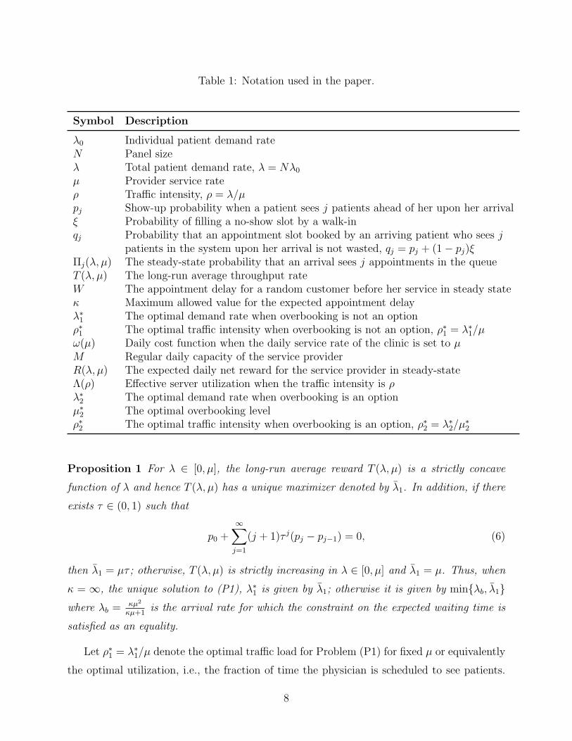
Table 1: Notation used in the paper.

Symbol Description

λ0 Individual patient demand rateN Panel sizeλ Total patient demand rate, λ = Nλ0

µ Provider service rateρ Traffic intensity, ρ = λ/µpj Show-up probability when a patient sees j patients ahead of her upon her arrivalξ Probability of filling a no-show slot by a walk-inqj Probability that an appointment slot booked by an arriving patient who sees j

patients in the system upon her arrival is not wasted, qj = pj + (1− pj)ξΠj(λ, µ) The steady-state probability that an arrival sees j appointments in the queueT (λ, µ) The long-run average throughput rateW The appointment delay for a random customer before her service in steady stateκ Maximum allowed value for the expected appointment delayλ∗1 The optimal demand rate when overbooking is not an option

ρ∗1 The optimal traffic intensity when overbooking is not an option, ρ∗1 = λ∗1/µ

ω(µ) Daily cost function when the daily service rate of the clinic is set to µM Regular daily capacity of the service providerR(λ, µ) The expected daily net reward for the service provider in steady-stateΛ(ρ) Effective server utilization when the traffic intensity is ρλ∗2 The optimal demand rate when overbooking is an option

µ∗2 The optimal overbooking level

ρ∗2 The optimal traffic intensity when overbooking is an option, ρ∗2 = λ∗2/µ

∗2

Proposition 1 For λ ∈ [0, µ], the long-run average reward T (λ, µ) is a strictly concave

function of λ and hence T (λ, µ) has a unique maximizer denoted by λ1. In addition, if there

exists τ ∈ (0, 1) such that

p0 +∞∑j=1

(j + 1)τ j(pj − pj−1) = 0, (6)

then λ1 = µτ ; otherwise, T (λ, µ) is strictly increasing in λ ∈ [0, µ] and λ1 = µ. Thus, when

κ = ∞, the unique solution to (P1), λ∗1 is given by λ1; otherwise it is given by min{λb, λ1}

where λb =κµ2

κµ+1is the arrival rate for which the constraint on the expected waiting time is

satisfied as an equality.

Let ρ∗1 = λ∗1/µ denote the optimal traffic load for Problem (P1) for fixed µ or equivalently

the optimal utilization, i.e., the fraction of time the physician is scheduled to see patients.

8

One important observation we can make from Proposition 1 is that the walk-in probability

ξ has no effect on the optimal panel size.

If there is no restriction on the expected delay, i.e., κ = ∞, the optimal traffic load is

independent of the service capacity. In this case, when the appointment delays do not have

a significant impact on customers’ show-up probabilities, we have ρ∗1 = 1. If, however, the

no-show rate drops fast as the appointment delay increases, then there exists an optimal

arrival rate, which is strictly less than the service rate, i.e., ρ∗1 < 1. Thus, even when there

is no restriction on the expected waiting time, the service provider does not prefer demand

to be as high as possible since high demand would lead to long waiting times, which in turn

would result in low show-up rates diminishing the system reward rate. Low demand rates

would lead to high show-up rates, but clearly, the service provider would not want to set it

so low as to cause the server idle frequently. Thus, there is an ideal value for the arrival rate

(an ideal panel size for a healthcare clinic) that helps the system hit the “right” balance.

2.3 Effects of introducing policies to improve show-up probabili-ties

In this section, we investigate how the panel size should be adjusted in response to the adop-

tion of a new policy, which is expected to change customers’ show-up rate. As we discussed

in Section 1, such policies include making reminder phone calls, sending text messages or

email reminders, providing financial incentives, and charging no-show fees. Specifically, we

investigate how the optimal panel size changes with the show-up probabilities p = {pj}∞j=0.

Consider the service system described in Section 2.1 with show-up probabilities denoted

by {pj}∞j=0. Suppose that once the new policy is adopted, the only change will be in customer

show-up probabilities, which we will denote by {pj}∞j=0. Also, suppose that once the new

policy is adopted, customers are more likely to show-up, i.e., pj ≥ pj for all j ∈ Z. Now,

when is the optimal panel size larger, before the new policy takes effect or after? More

precisely, letting λ∗1 denote the optimal arrival rate when show up probabilities are given by

{pj}∞j=0, which one is larger, λ∗1 or λ∗

1?

There are two different ways of coming up with an answer to this question based on intu-

ition. First, if patients are more likely to show up under the new policy, i.e., the probability

of showing up is higher for any given queue length, the provider might tend to believe that

the clinic can handle more patients effectively (after all there is less loss of efficiency due to

no-shows) and choose to increase its panel size. Alternatively, one might argue that because

9

patients are more likely to show up, the expected load per patient on the system is higher

and thus there is less incentive to admit more patients. Consequently, the optimal panel size

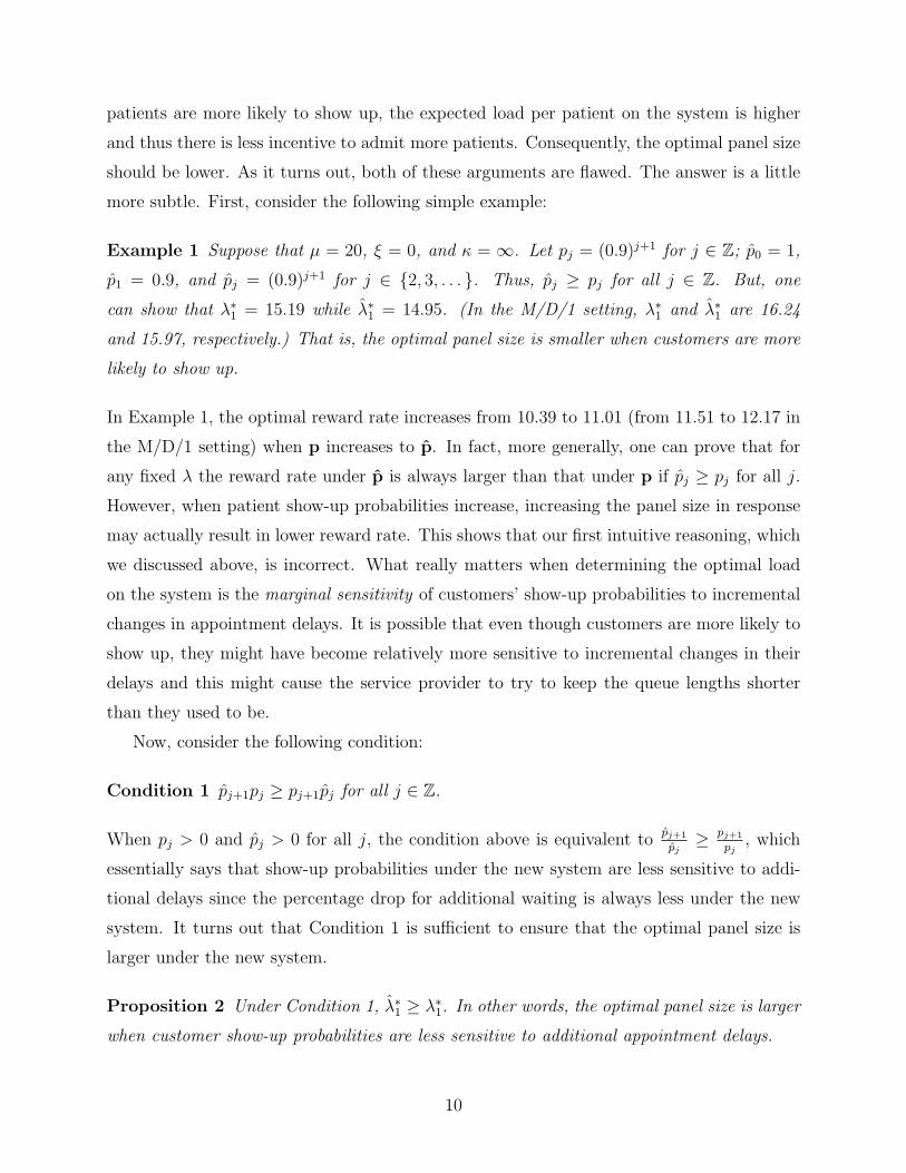
should be lower. As it turns out, both of these arguments are flawed. The answer is a little

more subtle. First, consider the following simple example:

Example 1 Suppose that µ = 20, ξ = 0, and κ = ∞. Let pj = (0.9)j+1 for j ∈ Z; p0 = 1,

p1 = 0.9, and pj = (0.9)j+1 for j ∈ {2, 3, . . . }. Thus, pj ≥ pj for all j ∈ Z. But, one

can show that λ∗1 = 15.19 while λ∗

1 = 14.95. (In the M/D/1 setting, λ∗1 and λ∗

1 are 16.24

and 15.97, respectively.) That is, the optimal panel size is smaller when customers are more

likely to show up.

In Example 1, the optimal reward rate increases from 10.39 to 11.01 (from 11.51 to 12.17 in

the M/D/1 setting) when p increases to p. In fact, more generally, one can prove that for

any fixed λ the reward rate under p is always larger than that under p if pj ≥ pj for all j.

However, when patient show-up probabilities increase, increasing the panel size in response

may actually result in lower reward rate. This shows that our first intuitive reasoning, which

we discussed above, is incorrect. What really matters when determining the optimal load

on the system is the marginal sensitivity of customers’ show-up probabilities to incremental

changes in appointment delays. It is possible that even though customers are more likely to

show up, they might have become relatively more sensitive to incremental changes in their

delays and this might cause the service provider to try to keep the queue lengths shorter

than they used to be.

Now, consider the following condition:

Condition 1 pj+1pj ≥ pj+1pj for all j ∈ Z.

When pj > 0 and pj > 0 for all j, the condition above is equivalent topj+1

pj≥ pj+1

pj, which

essentially says that show-up probabilities under the new system are less sensitive to addi-

tional delays since the percentage drop for additional waiting is always less under the new

system. It turns out that Condition 1 is sufficient to ensure that the optimal panel size is

larger under the new system.

Proposition 2 Under Condition 1, λ∗1 ≥ λ∗

1. In other words, the optimal panel size is larger

when customer show-up probabilities are less sensitive to additional appointment delays.

10

Proposition 2 makes it clear that what matters for the panel size decision is the customers’

sensitivity to delays. In Example 1, Condition 1 holds in the opposite direction becausepj+1

pj= 0.9, but

pj+1

pj= 0.9 for j = 0, 2, 3, . . . and p2

p1= 0.81. Therefore, it is not surprising

for the optimal panel size to drop under the new show-up probabilities. Proposition 2 also

implies that the intuitive argument that the optimal panel size should decrease when show-up

probabilities increase is incorrect because one can easily come up with examples in which the

show-up probabilities satisfy Condition (1) and pj ≥ pj for all j.

In short, our analysis in this section suggests that with a new intervention that is strongly

expected to improve patient show-up rates, providers would realize higher patient throughput

if they do not change their panel size. However, one should be careful when choosing a new

panel size in order to further benefit from changes in show-up probabilities since changes

based on one’s intuition alone might be counterproductive. It appears that, it is particularly

important for the service provider to get a good sense of how the customers’ sensitivities

to additional delays will change with the new intervention. If the intervention helps reduce

customer sensitivity to additional delays, then our results suggest that there is room for

further improvement in throughput by increasing the panel size.

3 Joint Panel Size and Overbooking Level Decisions

One approach clinics use in order to improve the utilization of the appointment slots is

to book more appointments than the clinic’s regular daily capacity typically allows. In this

section, we assume that in addition to the panel size, the service provider can also choose the

number of appointments scheduled per day. We model this in a stylized manner by making

service rate (i.e., number of appointments scheduled per day) another decision variable in

addition to the arrival rate.

3.1 Description of the model

The assumptions regarding the arrival of the appointment requests, service, and customer

no-show behavior are the same as those for the model described in Section 2.1. In order

to integrate overbooking and panel size decisions, we adopt a reward/cost formulation that

is similar to the one used in Liu et al. (2010). Specifically, we assume that for every filled

appointment slot, the service provider collects a nominal reward. The daily cost incurred

to the clinic is a function of the service rate µ it sets, i.e., the number of appointments

11

scheduled per day. We use ω(µ) to represent this cost function. We assume that there is a

fixed cost of operating the clinic independently of the service rate chosen by the clinic and

we assume that this cost is zero without loss of generality. As for the variable cost, we let

M ≥ 0 be the regular daily capacity of the clinic and thus max{0, µ −M} can be thought

of as the overbooking level. We assume that there is a cost if the clinic chooses to go above

this capacity. This cost can be seen as the direct financial cost (e.g., overtime cost for the

staff) and/or the indirect cost of patient dissatisfaction as a result of long waits on the day of

the appointment and less time devoted to the care of each patient. Intuitively, the more the

clinic overbooks, the higher this cost would be; in addition, it seems reasonable to assume

that this cost increases faster at a higher overbooking level. Thus, we assume that ω(µ) = 0

if µ ≤ M , ω(·) is continuous on [0,∞), strictly increasing and strictly convex on [M,∞),

and twice differentiable on (M,∞).

Let R(λ, µ) denote the expected daily net reward for the service provider. Then,

R(λ, µ) = T (λ, µ)− ω(µ) = (1− ξ)λ∞∑j=0

(1− ρ)ρjpj + µξ − ω(µ) (7)

where T (λ, µ) is given by (4). The objective of the service provider is to choose the arrival

and service rates which maximize R(λ, µ) while enforcing the expected appointment delay

to remain below a certain level κ. Then, our problem (P2) can be written as

maxλ,µ:0≤λ≤µ R(λ, µ)s.t. E(W ) ≤ κ

(P2)

with R(µ, µ) defined as R(µ, µ) = limλ→µR(λ, µ) = µq∞ − ω(µ) and limλ→µE(W ) = ∞.

3.2 Characterization of the optimal solution

In this section, we establish some structural properties of the optimal solution to Problem

(P2). We first study the model without the service level constraint, i.e., setting κ = ∞. We

know from Proposition 1 that for a fixed µ, there exists a unique value of λ that maximizes

the reward T (λ, µ). We denote this optimal value by λ(µ). Then, maximizing R(λ, µ) with

respect to λ and µ is equivalent to maximizing R(λ(µ), µ) with respect to µ only.

Let λ2 and µ2 denote the optimal values for λ and µ in Problem (P2) without the waiting

time constraint. From Lemma 2, which is provided in the Appendix, we know that for

0 ≤ µ ≤ M , R(λ(µ), µ) is a linear and strictly increasing function of µ, which immediately

implies that the optimal service rate is no less than the regular daily capacity, i.e., µ2 ≥ M .

12

This is not surprising since there is no incentive for the service provider not to use the

capacity that is already available with zero additional cost. In order to derive a complete

characterization of λ2 and µ2, we rewrite the reward function T (λ, µ) as follows

T (λ, µ) = µΛ(ρ),

where

Λ(ρ) = (1− ξ)∞∑j=0

(1− ρ)ρj+1pj + ξ. (8)

Hence Λ(ρ) can be regarded as the “effective” server utilization (proportion of time the server

is busy with serving patients, either scheduled ones who actually show up or walk-ins) when

the traffic intensity, λ/µ equals ρ.

Let ω+(µ) denote the right derivative of ω(µ). Then, ω+(µ) is a strictly increasing func-

tion for µ ∈ [M,∞) and it has an inverse, denoted by (ω+)−1(·), which is also strictly

increasing in its domain. Let ρ1 denote the optimal traffic intensity for Problem (P1) when

κ = ∞. Recall that ρ1 does not depend on µ. Hence, Λ(ρ1) is the effective server utilization

when system throughput (i.e., long-run average rate at which patients are served) is max-

imized when there is no restriction on the expected waiting time. Then we can prove the

following proposition.

Proposition 3 Suppose that κ = ∞, i.e., there is no restriction on the expected appointment

delay. Then, given the show-up probability vector p = {pj}∞j=0, the optimal service rate µ2

and arrival rate λ2 for Problem (P2) take the following form:

µ2 =

∞ if ω+(µ) ≤ Λ(ρ1), ∀µ ≥ M ,M if ω+(M) ≥ Λ(ρ1),

(ω+)−1(Λ(ρ1)) otherwise,

and λ2 = ρ1µ2. Furthermore, (λ2, µ2) is the unique optimal solution to problem (P2).

The expression for µ2 provided in Proposition 3 may seem technical but in fact it has

a straightforward interpretation. Notice that ω+(µ) is the marginal cost of additional unit

capacity when the service capacity is µ. The service provider would be willing to increase

the service capacity (and the arrival rate along with it) up to the point where marginal

cost equals the rate with which the system generates revenue, which is equal to the effective

server utilization. This corresponds to the third case in the statement for µ2 in Proposition

3. However, if the marginal cost is below this revenue generation rate no matter what the

13

service capacity is (which is unlikely in practice), then there is no point in restricting the

number of people to be seen on a given day and thus µ2 = ∞. If the marginal cost is higher

even at the regular capacity, then there is no incentive to overbook and thus µ2 = M .

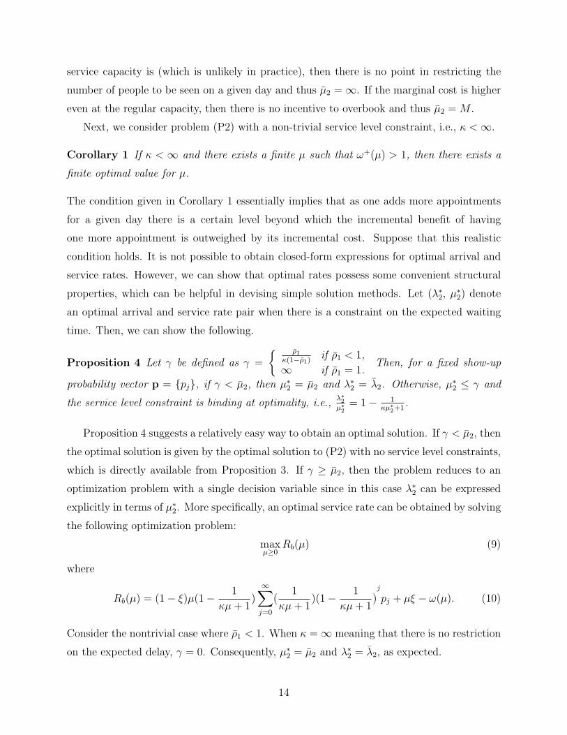
Next, we consider problem (P2) with a non-trivial service level constraint, i.e., κ < ∞.

Corollary 1 If κ < ∞ and there exists a finite µ such that ω+(µ) > 1, then there exists a

finite optimal value for µ.

The condition given in Corollary 1 essentially implies that as one adds more appointments

for a given day there is a certain level beyond which the incremental benefit of having

one more appointment is outweighed by its incremental cost. Suppose that this realistic

condition holds. It is not possible to obtain closed-form expressions for optimal arrival and

service rates. However, we can show that optimal rates possess some convenient structural

properties, which can be helpful in devising simple solution methods. Let (λ∗2, µ

∗2) denote

an optimal arrival and service rate pair when there is a constraint on the expected waiting

time. Then, we can show the following.

Proposition 4 Let γ be defined as γ =

{ ρ1κ(1−ρ1)

if ρ1 < 1,

∞ if ρ1 = 1.Then, for a fixed show-up

probability vector p = {pj}, if γ < µ2, then µ∗2 = µ2 and λ∗

2 = λ2. Otherwise, µ∗2 ≤ γ and

the service level constraint is binding at optimality, i.e.,λ∗2

µ∗2= 1− 1

κµ∗2+1

.

Proposition 4 suggests a relatively easy way to obtain an optimal solution. If γ < µ2, then

the optimal solution is given by the optimal solution to (P2) with no service level constraints,

which is directly available from Proposition 3. If γ ≥ µ2, then the problem reduces to an

optimization problem with a single decision variable since in this case λ∗2 can be expressed

explicitly in terms of µ∗2. More specifically, an optimal service rate can be obtained by solving

the following optimization problem:

maxµ≥0

Rb(µ) (9)

where

Rb(µ) = (1− ξ)µ(1− 1

κµ+ 1)

∞∑j=0

(1

κµ+ 1)(1− 1

κµ+ 1)j

pj + µξ − ω(µ). (10)

Consider the nontrivial case where ρ1 < 1. When κ = ∞ meaning that there is no restriction

on the expected delay, γ = 0. Consequently, µ∗2 = µ2 and λ∗

2 = λ2, as expected.

14

Since Rb(µ) defined in (10) is not necessarily unimodal in µ, multiple optimal solutions

may exist. Therefore, in the following, we shall refer to µ∗2 as the smallest optimal service

rate, i.e., µ∗2 = inf{µo : Rb(µ

o) ≥ Rb(µ) for all µ ≥ 0}. Then, we know from Proposition 4

that the corresponding optimal arrival rate λ∗2 and the optimal traffic load defined as ρ∗2 =

λ∗2

µ∗2

are also the smallest choices for these two variables.

3.3 Effects of introducing policies for improving show-up proba-bilities and changing the service level requirement

In this section, we investigate the sensitivity of the optimal panel size and overbooking

decisions (optimal arrival and service rates in our formulation) to customers’ show-up prob-

abilities and κ, the service level requirement on the expected waiting time. In Section 2.3,

we showed that when overbooking is not an option and there is a fixed daily capacity, the

optimal panel size is larger when customers’ show-up probabilities are less sensitive to ad-

ditional delays. When overbooking level is also a decision variable together with the panel

size, it is not clear how “improvements” in show-up probabilities would affect the optimal

decisions. When show-up rates of appointment slots are less sensitive to additional delays,

does that mean that the service provider has less incentive to overbook since there is less

uncertainty regarding whether or not the scheduled appointments will actually be filled?

As for the panel size, if the optimal overbooking level is higher, intuition suggests that the

optimal panel size would be larger as well but it is difficult to predict how it would change

otherwise. In any case, we find that the optimal panel size and overbooking level might

change in unpredictable ways.

We first investigate the sensitivity of the optimal decisions to show-up probabilities.

As in Section 2.3, suppose that as a result of a new policy that aims to improve show-up

rates, customer show-up probabilities {pj}∞j=0 become {pj}∞j=0 and let λ∗2 and µ∗

2 respectively

denote the optimal demand and service rates under this new policy (the smallest optimal

values in the unlikely event that there are multiple optimal solutions). Then, we can prove

the following proposition:

Proposition 5 If pj ≥ pj for all j ∈ Z, then µ∗2 ≥ µ∗

2. If pj ≥ pj for all j ∈ Z and Condition

1 holds (i.e., pj+1pj ≥ pj+1pj for all j ∈ Z), then λ∗2 ≥ λ∗

2, µ∗2 ≥ µ∗

2, and ρ∗2 ≥ ρ∗2, where

ρ∗2 =λ∗2

µ∗2and ρ∗2 =

λ∗2

µ∗2.

15

Remark 1 In the second part of Proposition 5, it is sufficient to assume that p0 ≥ p0

(instead of pj ≥ pj for all j ∈ Z) together with Condition 1.

According to Proposition 5, if customers are more likely to show up under the new policy,

the service provider chooses to increase the overbooking level. There is a cost of working

with a higher overbooking level but the service provider knows that appointment slots are

more likely to be filled in and thus the system is more likely to benefit from an increase

in the capacity. However, it turns out that even if the service provider chooses to work at

a higher overbooking level, it does not mean that she would choose to work with a larger

panel as well (see Example 2 below). A larger panel size and a higher overbooking level are

not guaranteed to be optimal when customers are more likely to show up. These show-up

rates also need to be less delay sensitive for the service provider to choose both a higher

overbooking level and a larger panel size.

Example 2 Suppose that p0 = 0.4 and pj = 0.38 for all j ≥ 1, and p0 = 1 and pj = 0.4

for all j ≥ 1. Let ξ = 0, κ = ∞ and ω(µ) = aµ2 where a is a positive constant. Then,

T (λ, µ) = λ[0.4(1−ρ)+0.38ρ] = µ(0.4ρ−0.02ρ2). For a fixed µ, T (λ, µ) is strictly increasing

in ρ ∈ [0, 1]. Hence ρ1 = 1 and R(λ(µ), µ) = 0.38µ − aµ2. It then follows that λ∗2 = µ∗

2 =

19100a

. Now, note that T (λ, µ) = λ[(1 − ρ) + 0.4ρ] = µ(ρ − 0.6ρ2). Hence λ∗2 = 5

6µ∗2, and

R(λ(µ), µ) = 512µ − aµ2. It follows that µ∗

2 = 524a

> µ∗2 = 19

100aas expected since pj > pj for

all j; however, λ∗2 =

56× 5

24a= 25

144a< λ∗

2 =19

100aand ρ∗2 =

56< 1 = ρ∗2.

Next, we investigate how changes in the service level requirement, which is determined

by κ, affect the optimal decisions. For example, if the service provider commits herself to

providing customers shorter waiting times, how should she adjust the panel size and the

daily overbooking level? Intuition suggests that because the goal is to reduce the average

waiting time, a reasonable adjustment would be to reduce the panel size and increase the

overbooking level appropriately. Interestingly however, that is not necessarily the case. As

an example, suppose that pj = 0.99j for j ∈ Z and ω(µ) = 0.01µ2. In this case, Figure 1

shows how the optimal demand rate λ∗2, the optimal service rate µ∗

2, and the optimal traffic

load ρ∗2 =λ∗2

µ∗2change with the service level parameter κ which varies from 0.07 to 0.27. Recall

that κ is the allowable maximum value set by the provider for the average waiting time of

scheduled customers. One can observe that the optimal arrival rate and service rate are not

monotone in κ. Interestingly, for small values of κ, the optimal decision is to increase the

16

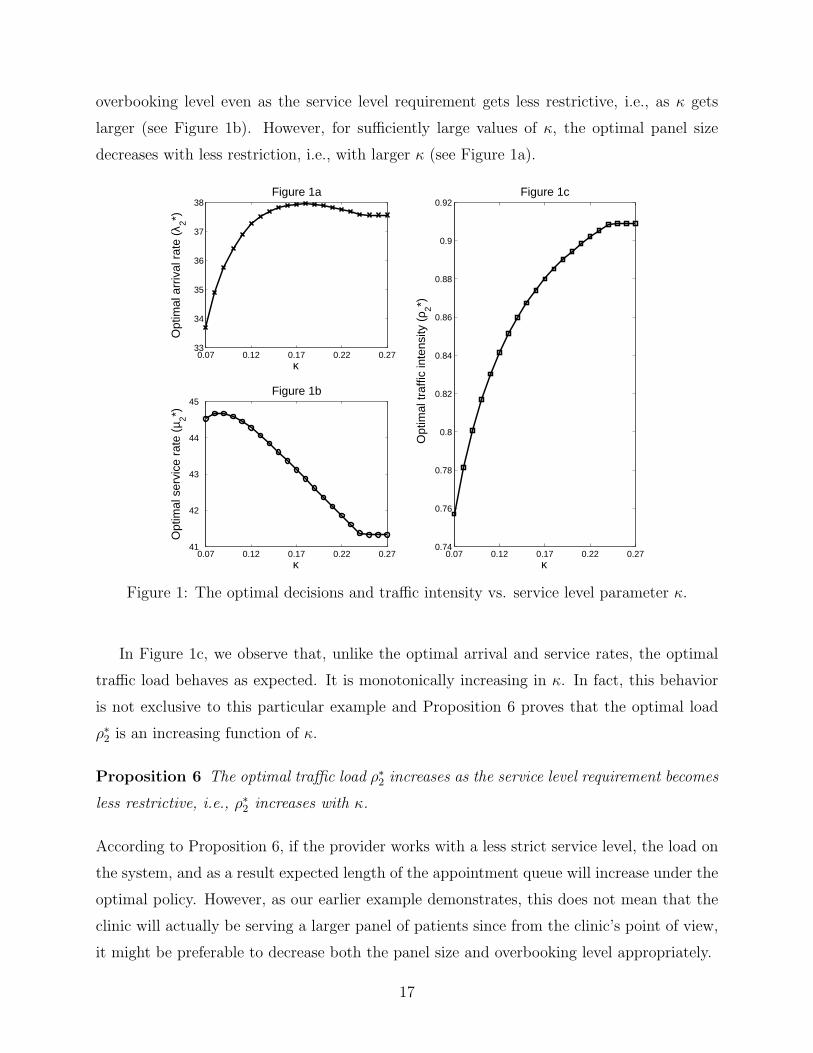
overbooking level even as the service level requirement gets less restrictive, i.e., as κ gets

larger (see Figure 1b). However, for sufficiently large values of κ, the optimal panel size

decreases with less restriction, i.e., with larger κ (see Figure 1a).

0.07 0.12 0.17 0.22 0.2733

34

35

36

37

38

κ

Opt

imal

arr

ival

rat

e (λ

2*)Figure 1a

0.07 0.12 0.17 0.22 0.2741

42

43

44

45

κ

Opt

imal

ser

vice

rat

e (µ

2*)

Figure 1b

0.07 0.12 0.17 0.22 0.270.74

0.76

0.78

0.8

0.82

0.84

0.86

0.88

0.9

0.92

κ

Opt

imal

traf

fic in

tens

ity (

ρ 2*)

Figure 1c

Figure 1: The optimal decisions and traffic intensity vs. service level parameter κ.

In Figure 1c, we observe that, unlike the optimal arrival and service rates, the optimal

traffic load behaves as expected. It is monotonically increasing in κ. In fact, this behavior

is not exclusive to this particular example and Proposition 6 proves that the optimal load

ρ∗2 is an increasing function of κ.

Proposition 6 The optimal traffic load ρ∗2 increases as the service level requirement becomes

less restrictive, i.e., ρ∗2 increases with κ.

According to Proposition 6, if the provider works with a less strict service level, the load on

the system, and as a result expected length of the appointment queue will increase under the

optimal policy. However, as our earlier example demonstrates, this does not mean that the

clinic will actually be serving a larger panel of patients since from the clinic’s point of view,

it might be preferable to decrease both the panel size and overbooking level appropriately.

17

Finally, in this section we investigate how the optimal panel size and overbooking level

change with walk-in probability ξ. When overbooking is not an option, we found that the

walk-in probability has no effect on the optimal panel size. However, it turns out that when

overbooking is an option, higher walk-in probabilities not only lead to higher overbooking

levels but also larger panel sizes and traffic intensities.

Proposition 7 When ξ increases, the optimal demand rate λ∗2, the optimal overbooking level

µ∗2 and the optimal traffic intensity ρ∗2 for problem (P2) increase.

When the probability that an appointment slot is not wasted is higher, overbooking is

more likely to benefit the clinic and thus the optimal overbooking level is higher. This

result may seem counterintuitive at first. After all one reason clinics overbook is to alleviate

the effect of no-shows on the system. However, one should note that the increase in the

overbooking level is mainly due to the fact that the panel size is also a decision variable.

When the overbooking level is higher the clinic can handle more patients on a daily basis and

therefore the optimal panel size is also larger. In fact, it turns out that the fractional change

in the optimal panel size is larger than the fractional change in the optimal overbooking

level, leading to a larger traffic load. When the no-show slots are more likely to be filled in

by walk-ins, the clinic can handle a larger load efficiently.

In summary, lower no-show rates will always help if one is willing to keep the same

panel size and overbooking level. There is room for further improvement if the provider

is willing to make some changes. However, our analysis in this section suggests that one

needs to be careful when choosing a new panel size and overbooking level as it might have

some unexpected consequences. For example, even though a lower no-show rate encourages

the provider to see more patients in a day, it does not mean that the provider should

increase the panel size. Only when patient sensitivity to additional delays also decreases,

a larger panel size would necessarily be more beneficial. On a separate note, our results

also point to interesting relationships among expected appointment delay (the service level

requirement), optimal panel size, and overbooking level. As it turns out, requiring the

expected appointment delay to be lower may lead to a larger optimal panel size or a lower

overbooking level.

Before we move on to the description and discussion of our numerical study, it might be

helpful to provide a summary of our key analytical findings established in Sections 2 and

3. In particular, Table 2 sorts out the conditions needed for the optimal panel size and

18

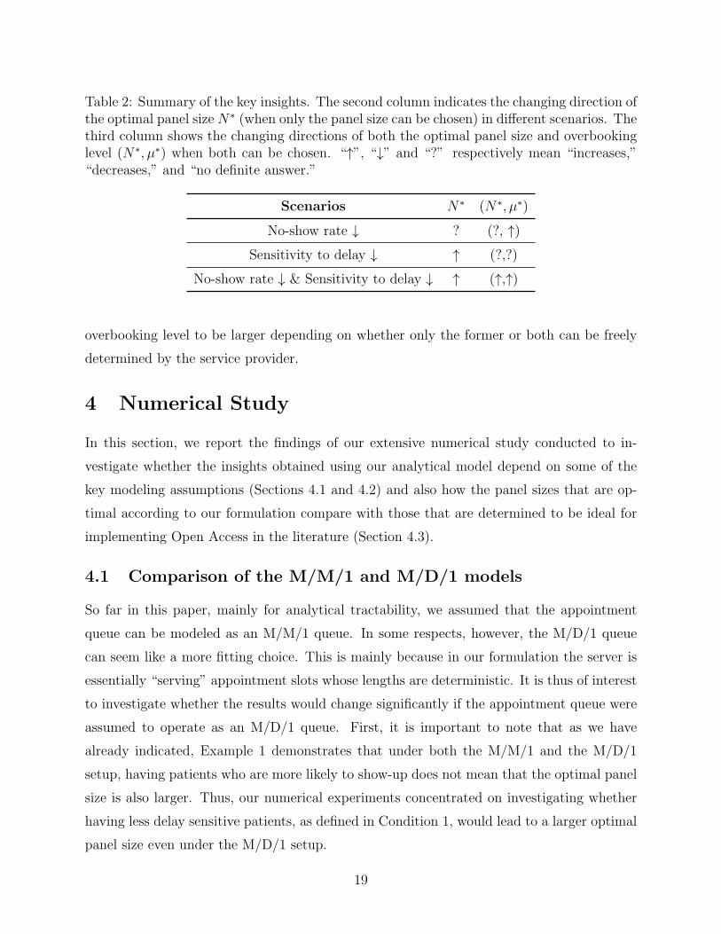
Table 2: Summary of the key insights. The second column indicates the changing direction ofthe optimal panel size N∗ (when only the panel size can be chosen) in different scenarios. Thethird column shows the changing directions of both the optimal panel size and overbookinglevel (N∗, µ∗) when both can be chosen. “↑”, “↓” and “?” respectively mean “increases,”“decreases,” and “no definite answer.”

Scenarios N∗ (N∗, µ∗)

No-show rate ↓ ? (?, ↑)

Sensitivity to delay ↓ ↑ (?,?)

No-show rate ↓ & Sensitivity to delay ↓ ↑ (↑,↑)

overbooking level to be larger depending on whether only the former or both can be freely

determined by the service provider.

4 Numerical Study

In this section, we report the findings of our extensive numerical study conducted to in-

vestigate whether the insights obtained using our analytical model depend on some of the

key modeling assumptions (Sections 4.1 and 4.2) and also how the panel sizes that are op-

timal according to our formulation compare with those that are determined to be ideal for

implementing Open Access in the literature (Section 4.3).

4.1 Comparison of the M/M/1 and M/D/1 models

So far in this paper, mainly for analytical tractability, we assumed that the appointment

queue can be modeled as an M/M/1 queue. In some respects, however, the M/D/1 queue

can seem like a more fitting choice. This is mainly because in our formulation the server is

essentially “serving” appointment slots whose lengths are deterministic. It is thus of interest

to investigate whether the results would change significantly if the appointment queue were

assumed to operate as an M/D/1 queue. First, it is important to note that as we have

already indicated, Example 1 demonstrates that under both the M/M/1 and the M/D/1

setup, having patients who are more likely to show-up does not mean that the optimal panel

size is also larger. Thus, our numerical experiments concentrated on investigating whether

having less delay sensitive patients, as defined in Condition 1, would lead to a larger optimal

panel size even under the M/D/1 setup.

19

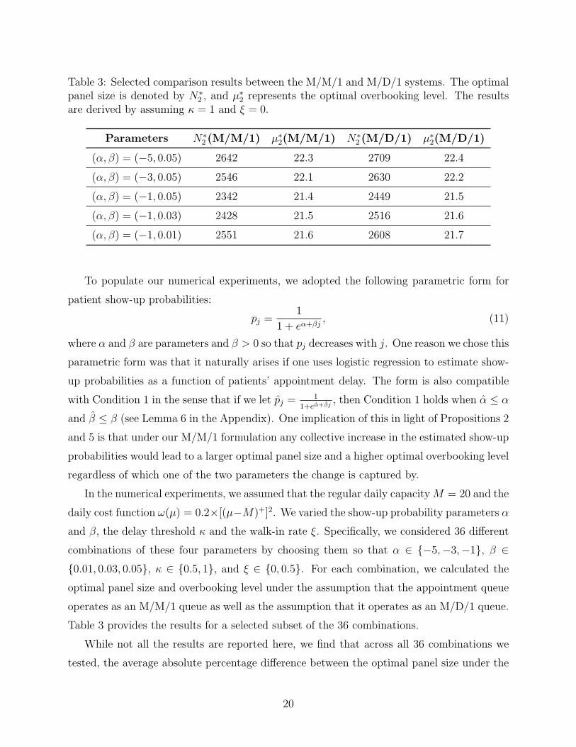
Table 3: Selected comparison results between the M/M/1 and M/D/1 systems. The optimalpanel size is denoted by N∗

2 , and µ∗2 represents the optimal overbooking level. The results

are derived by assuming κ = 1 and ξ = 0.

Parameters N∗2 (M/M/1) µ∗

2(M/M/1) N∗2 (M/D/1) µ∗

2(M/D/1)

(α, β) = (−5, 0.05) 2642 22.3 2709 22.4

(α, β) = (−3, 0.05) 2546 22.1 2630 22.2

(α, β) = (−1, 0.05) 2342 21.4 2449 21.5

(α, β) = (−1, 0.03) 2428 21.5 2516 21.6

(α, β) = (−1, 0.01) 2551 21.6 2608 21.7

To populate our numerical experiments, we adopted the following parametric form for

patient show-up probabilities:

pj =1

1 + eα+βj, (11)

where α and β are parameters and β > 0 so that pj decreases with j. One reason we chose this

parametric form was that it naturally arises if one uses logistic regression to estimate show-

up probabilities as a function of patients’ appointment delay. The form is also compatible

with Condition 1 in the sense that if we let pj =1

1+eα+βj, then Condition 1 holds when α ≤ α

and β ≤ β (see Lemma 6 in the Appendix). One implication of this in light of Propositions 2

and 5 is that under our M/M/1 formulation any collective increase in the estimated show-up

probabilities would lead to a larger optimal panel size and a higher optimal overbooking level

regardless of which one of the two parameters the change is captured by.

In the numerical experiments, we assumed that the regular daily capacityM = 20 and the

daily cost function ω(µ) = 0.2×[(µ−M)+]2. We varied the show-up probability parameters α

and β, the delay threshold κ and the walk-in rate ξ. Specifically, we considered 36 different

combinations of these four parameters by choosing them so that α ∈ {−5,−3,−1}, β ∈{0.01, 0.03, 0.05}, κ ∈ {0.5, 1}, and ξ ∈ {0, 0.5}. For each combination, we calculated the

optimal panel size and overbooking level under the assumption that the appointment queue

operates as an M/M/1 queue as well as the assumption that it operates as an M/D/1 queue.

Table 3 provides the results for a selected subset of the 36 combinations.

While not all the results are reported here, we find that across all 36 combinations we

tested, the average absolute percentage difference between the optimal panel size under the

20

M/M/1 setup and that under the M/D/1 setup is only 3.3%. That for the overbooking level

and the average net reward are only 0.23% and 2.98%, respectively. Furthermore, all the key

structural results obtained under the M/M/1 setup continue to hold under M/D/1 setup.

In particular, for any fixed combination of κ and ξ, the optimal panel size and overbooking

level in both cases are decreasing in α for fixed β and decreasing in β for fixed α.

4.2 Impact of customer cancellation and balking

One simplifying assumption we made in our mathematical analysis was that patients neither

cancel their appointments nor balk, i.e., choose not to join the appointment queue when they

find the appointment delay long. In this section, we investigate the effect of this simplification

on our key findings via simulation.

In our simulation model, we assumed that a patient who finds j scheduled appointments

in the queue, independently of the others, would choose to join the appointment queue with

probability e−ηj, where η > 0 is the parameter for balking intensity. This probability model

captures the fact that patients are more likely not to schedule an appointment when the

appointment queue/delay is longer. Note also that, a larger η indicates a higher likelihood

to balk for any given queue length j.

To model cancellations, we assumed that each patient who joined the appointment queue,

independently of the others and the system state, would choose to cancel her appointment

after some random amount of time that has exponential distribution. However, cancelation

only occurs if the patient has not received service until then. In line with what mostly

happens in practice, when an appointment is canceled, appointments that follow the can-

celed appointment are not rescheduled to fill in the newly vacated slot. Thus, the canceled

appointment slot leaves a “hole” in the queue leaving other scheduled appointments intact.

When a new appointment request arrives, rather than scheduling it at the end of the queue,

one of these holes is filled if there are any. Specifically, the patient is scheduled for the slot

that is closest to service. (If the first available slot happens to be the first one in the queue,

then the second hole in the queue is filled because the “service” for the first slot has already

started. This is to capture the fact that very late cancelations cannot be filled.) If there

are no holes in the queue, the appointment is scheduled at the end of the queue. As in the

previous section, patients who do not cancel their appointments, show up with probabilities

that follow the parametric form (11).

21

We considered three different balking intensities η ∈ {0, 0.001, 0.003} and three different

cancelation rates θ ∈ {0.1, 0.2, 0.5}. For each combination of η and θ, we varied the show-up

probability parameters. In particular, we chose α ∈ {−5,−1} and β ∈ {0.01, 0.05}. In order

to get a better sense of what exactly these choices mean, consider a provider who sees 20

patients per day. Then, when η = 0.001, for a patient who finds an appointment queue length

of 2 days, 5 days, and 10 days at the time of her arrival, the balking probability is respectively

4%, 10%, and 18%. When θ = 0.1, her cancelation probability before appointment is

respectively 18%, 39%, and 63%. Finally, when α = −5 and β = 0.01 her no-show probability

is respectively 1%, 2%, and 5%.

We assumed that the regular daily capacity M = 20, the daily cost function ω(µ) =

0.2× [(µ−M)+]2 and service times were deterministic. We also assumed there were no walk-

in patients and there is no restriction on the expected delay, i.e., ξ = 0 and κ = ∞. Thus,

in total, we considered 36 combinations for the choice of (η, θ, α, β). For each combination,

we varied the panel size N with a step size of 10 and the daily service capacity level µ with

a step size of 0.1, and ran simulation for each pair of (N,µ). We used the batch-means

method with a batch length of 3000 days and 11 batches, where the first batch was used as

the warm-up period. We computed the average reward for each pair of (N,µ) and named the

pair that gave the largest average reward the optimal solution. We summarize our results in

Table 4, where Cases 1 through 4 correspond to four different combinations of the show-up

probability parameters (α, β) = (−5, 0.01), (−5, 0.05), (−1, 0.01) and (−1, 0.05), respectively.

One can observe from Table 4 that the higher the balking intensity, the larger the optimal

panel size. This is not surprising because balking makes the appointment queue lengths (and

hence delays) shorter on average, which in turn means that patients are more likely to show-

up giving the clinic an incentive to increase its panel size. The effect of balking on the

overbooking level is more salient. We observe that, the optimal overbooking level does not

appear to have a monotone relationship with the balking intensity, most likely due to the

fact that the clinic has the flexibility to choose the panel size as well. The clinic can manage

different degrees of balking behavior by playing with the panel size appropriately but keeping

the overbooking level more or less constant.

As in the case of balking, a higher cancelation rate leads to a larger optimal panel size

(see Tables 3 and 4). However, the reader should note that in our simulation model, patients

who cancel their appointments do not reschedule, and thus cancellation has the effect of

reducing the load on the clinic and thereby enabling it to handle a lager panel of patients.

22

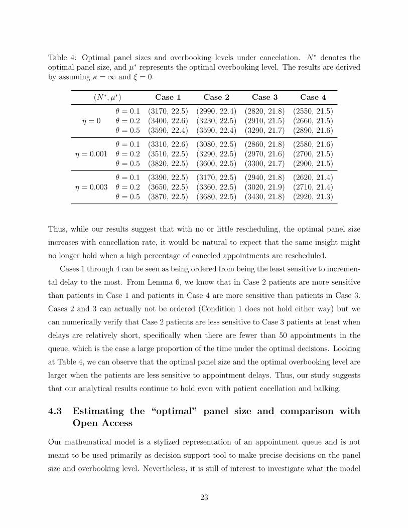
Table 4: Optimal panel sizes and overbooking levels under cancelation. N∗ denotes theoptimal panel size, and µ∗ represents the optimal overbooking level. The results are derivedby assuming κ = ∞ and ξ = 0.

(N∗, µ∗) Case 1 Case 2 Case 3 Case 4

η = 0θ = 0.1 (3170, 22.5) (2990, 22.4) (2820, 21.8) (2550, 21.5)θ = 0.2 (3400, 22.6) (3230, 22.5) (2910, 21.5) (2660, 21.5)θ = 0.5 (3590, 22.4) (3590, 22.4) (3290, 21.7) (2890, 21.6)

η = 0.001θ = 0.1 (3310, 22.6) (3080, 22.5) (2860, 21.8) (2580, 21.6)θ = 0.2 (3510, 22.5) (3290, 22.5) (2970, 21.6) (2700, 21.5)θ = 0.5 (3820, 22.5) (3600, 22.5) (3300, 21.7) (2900, 21.5)

η = 0.003θ = 0.1 (3390, 22.5) (3170, 22.5) (2940, 21.8) (2620, 21.4)θ = 0.2 (3650, 22.5) (3360, 22.5) (3020, 21.9) (2710, 21.4)θ = 0.5 (3870, 22.5) (3680, 22.5) (3430, 21.8) (2920, 21.3)

Thus, while our results suggest that with no or little rescheduling, the optimal panel size

increases with cancellation rate, it would be natural to expect that the same insight might

no longer hold when a high percentage of canceled appointments are rescheduled.

Cases 1 through 4 can be seen as being ordered from being the least sensitive to incremen-

tal delay to the most. From Lemma 6, we know that in Case 2 patients are more sensitive

than patients in Case 1 and patients in Case 4 are more sensitive than patients in Case 3.

Cases 2 and 3 can actually not be ordered (Condition 1 does not hold either way) but we

can numerically verify that Case 2 patients are less sensitive to Case 3 patients at least when

delays are relatively short, specifically when there are fewer than 50 appointments in the

queue, which is the case a large proportion of the time under the optimal decisions. Looking

at Table 4, we can observe that the optimal panel size and the optimal overbooking level are

larger when the patients are less sensitive to appointment delays. Thus, our study suggests

that our analytical results continue to hold even with patient cacellation and balking.

4.3 Estimating the “optimal” panel size and comparison withOpen Access

Our mathematical model is a stylized representation of an appointment queue and is not

meant to be used primarily as decision support tool to make precise decisions on the panel

size and overbooking level. Nevertheless, it is still of interest to investigate what the model

23

would suggest as the optimal panel size and how it would compare with panel sizes that are

recommended for Open Access implementation using data from an actual clinic.

To that end, in this section, we estimate the “throughput maximizing” panel size using

our model and compare our numbers with those suggested by Green and Savin (2008) for

Open Access implementation. To make a proper comparison, we use exactly the same data

and the same no-show estimates used in Green and Savin (2008). Specifically, we let the

individual appointment demand rate λ0 to be 0.008 per day and the service rate to be 20

customers per day, i.e., µ = 20. We use the following parametrical model for show-up

probabilities, pj, j ∈ Z:

pj = 1− (γmax − (γmax − γ0)e−⌊j/µ⌋/C)

where γ0 is the minimum observed no-show rate, γmax is the maximum observed no-show

rate, and C is the no-show backlog sensitivity parameter. Using data from a Magnetic

Resonance Imaging (MRI) facility, Green and Savin (2008) estimated γ0, γmax, and C to be

0.01, 0.31, and 50, respectively. Using these estimates, we find that the optimal panel size

under the M/M/1 setup is 2459 while that under the M/D/1 setup is 2471. The M/M/1

model estimate simply uses λ1 obtained through Proposition 1; the M/D/1 model estimate

is obtained by numerically maximizing T (λ, 20) as defined in (2) under the assumptions of

Poisson arrivals and deterministic service times with the queue length truncated at 1000.

As we discussed before, the goal of Green and Savin (2008) is to estimate the ideal panel

size for Open Access, i.e., the panel size that will keep the clinic “in balance” for Open Access

implementation. Using four different models (M/D/1/K, M/M/1/K, and two simulation

models) and four different desired values for the same-day appointment probability, they

obtained 16 different panel size estimates ranging from 2205 to 2368. Our throughput max-

imizing panel size estimates are larger than what Green and Savin (2008) suggest for Open

Access. This is not surprising mainly due to two reasons. First, having to provide same-day

service forces the service provider to keep the panel sizes smaller. Second, our model as-

sumes that no-show customers do not reschedule new appointments while Green and Savin

(2008) assumed that all no-show customers immediately scheduled a new appointment. Since

rescheduling means more work load per customer, it leads to a smaller optimal panel size.

One question of interest is the secondary effects of using a throughput maximizing panel

size. The clinic might be maximizing throughput, but how about the effect on the delays

the patients experience? Do they wait for a long time, at least significantly longer than they

24

Table 5: Computed values for the key performance measures under the M/M/1 model withno rescheduling. E(Q) is the average appointment queue length. E(W ) is the averagepatient appointment delay. PS is the probability that an arriving appointment request isaccommodated in the same day. PT is the probability that an arriving appointment requestis accommodated within the next two days.

Panel Size Throughput E(Q) E(W ) PS PT

2220 17.572 7.929 0.396 0.907 0.991

2300 18.191 11.500 0.575 0.811 0.964

2380 18.783 19.833 0.992 0.626 0.860

2460 19.194 60.877 3.043 0.276 0.476

2540 18.134 338.191 16.860 0.000 0.002

would under the same-day scheduling policy? Table 5 clearly demonstrates the trade-off

among system throughput, customer delays, and the fraction of customers who can book

appointments within a day or two. To be able to make a more meaningful comparison,

following Green and Savin (2008), we truncate the queue length at 400 here, i.e., we assume

an M/M/1/K queue with K = 400 instead of an M/M/1 queue. This does not affect the

results in the first four rows in the table significantly; however, it is necessary for the last

row since otherwise, the queue would have been unstable.

In Table 5, the maximum throughput is 19.194 with a panel size of 2460. In this case,

the average appointment delay is 3 days (since the daily service rate is 20 patients) and

approximately 28% of the patients can be seen on the day they call for an appointment. The

clinic can improve the waiting times and same-day access probabilities by reducing the panel

size. For example, if the panel size is 2220, approximately 90% of the customers can get

same-day appointments, but the throughput drops to about 17.572. This is more than an

8% decrease, which suggests that committing to same-day appointments may not be optimal

from a system efficiency point of view. If the clinic is interested in providing a high service

level and throughput is a secondary concern, then same-day appointment scheduling could

work well. If efficiency is more important, it might pay off to be more flexible. One can still

stick with Open Access but perhaps implement it a little less strictly by promising customers

appointments within two or three days as opposed to the same day.

25

5 Conclusion

This paper uses stylized models to investigate the relationships between patients’ no-show

behavior and the optimal panel size and overbooking decisions. Our results provide insights

particularly for clinics interested in reducing patient no-shows by behavioral interventions

such as sending reminders for appointments. These interventions typically improve patient

attendance but cannot eliminate no-shows completely. In general, clinics prefer higher show-

up probabilities, which not only mean less time wasted and more patients served, but also

help clinics make better operational decisions because of the reduced uncertainty. What

is far less clear is how clinics should alter their decisions in response to changes in patient

show-up probabilities. Our findings suggest that responses based on one’s intuition might

not work as expected. For example, having patients who are more likely to show-up does

not necessarily imply that the optimal panel size should be larger or smaller. What appears

to be more important is whether patients are more or less sensitive to additional delays.

Past empirical studies on the effectiveness of intervention policies have largely focused on

changes in no-show rates (Macharia et al. 1992, Guy et al. 2012), but did not investigate the

changes in the sensitivity of no-show probabilities to incremental changes in appointment

delays. This is an important avenue for future research.

The generic nature of our formulation allows us to generate insights without restricting

ourselves to any specific appointment scheduling policy, and our main finding, which says

that panel size decisions should be informed by the sensitivity of the show-up probabilities

to incremental changes in appointment delays is likely to hold under more general conditions

and various appointment scheduling schemes. Nevertheless, our formulation is stylized and

more research is needed to provide support for this claim. It is also important to note that

how exactly one defines “sensitivity to incremental delays” may need to be reconsidered if

one uses a more detailed formulation of an appointment system. Our Condition 1 in this

paper, however, can help in identifying similar conditions in other formulations. Thus, one

avenue for future work is to model clinics that use standard appointment scheduling policies

in more detail (for example by explicitly considering day and time of the appointment,

patient preferences etc.) and investigate the connection between optimal panel sizes and

show-up probabilities. Proving analytical results may not be possible, but investigation via

a simulation study would likely be fruitful.

26

References

Bean, A. G., J. Talaga. 1995. Predicting appointment breaking. Journal of Health Care

Marketing 15(1) 29–34.

Browder, A. 1996. Mathematical Analysis: An Introduction. Springer Verlag, New York,

New York.

Cayirli, T., E. Veral. 2003. Outpatient scheduling in health care: A review of literature.

Production and Operations Management 12(4) 519–549.

Daggy, J., M. Lawley, D. Willis, D. Thayer, C. Suelzer, P.C. DeLaurentis, A. Turkcan,

S. Chakraborty, L. Sands. 2010. Using no-show modeling to improve clinic performance.

Health Informatics Journal 16(4) 246–259.

Dreiher, J., M. Froimovici, Y. Bibi, D.A. Vardy, A. Cicurel, A.D. Cohen. 2008. Nonatten-

dance in obstetrics and gynecology patients. Gynecologic and Obstetric Investigation

66(1) 40–43.

Fleck, E. 2012. Director, Internal Medicine, NewYork-Presbyterian Hospital/Ambulatory

Care Network. Personal communication. July 19, 2012.

Gallucci, G., W. Swartz, F. Hackerman. 2005. Brief reports: Impact of the wait for an initial

appointment on the rate of kept appointments at a mental health center. Psychiatric

Services 56(3) 344–346.

Geraghty, M., F. Glynn, M. Amin, J. Kinsella. 2007. Patient mobile telephone text reminder:

a novel way to reduce non-attendance at the ENT out-patient clinic. The Journal of

Laryngology and Otology 122(3) 296–298.

Green, L. V., S. Savin. 2008. Reducing delays for medical appointments: A queueing ap-

proach. Operations Research 56(6) 1526–1538.

Grunebaum, M., P. Luber, M. Callahan, A.C. Leon, M. Olfson, L. Portera. 1996. Predictors

of missed appointments for psychiatric consultations in a primary care clinic. Psychiatric

Services 47(8) 848–852.

Gupta, D., B. Denton. 2008. Appointment scheduling in health care: Challenges and oppor-

tunities. IIE Transactions 40(9) 800–819.

Gupta, D., L. Wang. 2008. Revenue management for a primary-care clinic in the presence

of patient choice. Operations Research 56(3) 576–592.

27

Gupta, D., W.Y. Wang. 2012. Patient appointments in ambulatory care. Randolph Hall, ed.,

Handbook of Healthcare System Scheduling , International Series in Operations Research

and Management Science, vol. 168. Springer US, 65–104.

Guy, R., J. Hocking, H. Wand, S. Stott, H. Ali, J. Kaldor. 2012. How effective are short mes-

sage service reminders at increasing clinic attendance? a meta-analysis and systematic

review. Health Services Research 47(2) 614–632.

Hashim, M. J. P. Franks, K. Fiscella. 2001. Effectiveness of telephone reminders in improving

rate of appointments kept at an outpatient clinic: a randomized controlled trial. The

Journal of the American Board of Family Practice 14(3) 193–196.

Jones, RB, AJ Hedley. 1988. Reducing non-attendance in an outpatient clinic. Public Health

102(4) 385–391.

KC, Diwas, N. Osadchiy. 2012. Matching supply with demand in an outpatient clinic.

Working Paper. Emory University, Goizueta Business School, Atlanta, GA.

Kopach, R., P. C. DeLaurentis, M. Lawley, K. Muthuraman, L. Ozsen, R. Rardin, H. Wan,

P. Intrevado, X. Qu, D. Willis. 2007. Effects of clinical characteristics on successful open

access scheduling. Health Care Management Science 10(2) 111–124.

Kulkarni, V. G. 1995. Modeling and Analysis of Stochastic Systems . Chapman & Hall/CRC,

Boca Raton, FL.

LaGanga, L. R., S. R. Lawrence. 2007. Clinic overbooking to improve patient access and

increase provider productivity. Decision Sciences 38(2) 251–276.

Liu, N, S. Ziya, V. G. Kulkarni. 2010. Dynamic scheduling of outpatient appointments under

patient no-shows and cancellations. Manufacturing & Service Operations Management

12(2) 347–364.

Macharia, W. M., G. Leon, B. H. Rowe, B. J. Stephenson, R. B. Haynes. 1992. An overview

of interventions to improve compliance with appointment keeping for medical services.

The Journal of the American Medical Association 267(13) 1813–1817.

Moore, C. G., P. Wilson-Witherspoon, J. C. Probst. 2001. Time and money: Effects of

no-showsat a family practice residency clinic. Family Medicine 33(7) 522–527.

Norris, J.B., C. Kumar, S. Chand, H. Moskowitz, S.A. Shade, D.R. Willis. 2012. An empirical

investigation into factors affecting patient cancellations and no-shows at outpatient

clinics. Decision Support Systems .

28

Patrick, J., M. L. Puterman, M. Queyranne. 2008. Dynamic multi-priority patient scheduling

for a diagnostic resource. Operations Research 56(6) 1507–1525.

Pesata, V., G. Pallija, A. A. Webb. 1999. A descriptive study of missed appointments:

Families’ perceptions of barriers to care. Journal of Pediatric Health Care 13(4) 178–

182.

Rosenthal, D. 2011. Director of Behavioral Science of Center for Family and Community

Medicine at Columbia University. Personal communication. March 16, 2011.

Schutz, Hans-Jorg, Rainer Kolisch. 2012. Approximate dynamic programming for capacity

allocation in the service industry. European Journal of Operational Research 218(1)

239–250.

Shonick, W., B.W. Klein. 1977. An approach to reducing the adverse effects of broken ap-

pointments in primary care systems: development of a decision rule based on estimated

conditional probabilities. Medical Care 15(5) 419–429.

Ulmer, T., C. Troxler. 2004. The economic cost of missed appointments and the open access

system. Community Health Scholars. University of Florida, Gainsville, FL.

Wang, W.Y., D. Gupta. 2011. Adaptive appointment systems with patient preferences.

Manufacturing & Service Operations Management 13(3) 373–389.

29

Online Supplement for “Panel Size and Overbooking Decisions forAppointment-based Services under Patient No-shows”

Throughout the appendix, for a given function f(·), we use the notation f ′(·) and f ′′(·)to denote the first and second derivatives of f(·) unless otherwise specified.

Online Appendix - Proofs of the Results

Lemma 1

limλ→µ

T (λ, µ) = limλ→µ

[(1− ξ)λ∞∑j=0

(1− ρ)ρjpj + µξ] = µ[ξ + (1− ξ)p∞].

Proof of Lemma 1:

It suffices to show that limλ→µ λ∑∞

j=0(1 − ρ)ρjpj = µp∞, which is equivalent to show that

limρ→1 µ∑∞

j=0(1−ρ)ρj+1pj = µp∞. To further simplify the proof, we only need to show that,

limρ→1

∞∑j=0

(1− ρ)ρjpj = p∞,

since limρ→1 ρ = 1.

Now, fix an arbitrary ϵ > 0. Since {pj, j = 0, 1, 2, . . . } is a non-increasing sequence and

limj→∞ pj = p∞, there exists a positive integer K such that pj − p∞ < 12ϵ for all j ≥ K + 1.

Pick a ρ′ ∈ (0, 1) such that 1− ρK+1 < 12ϵ for all ρ ∈ [ρ′, 1). It then follows that, ∀ρ ∈ [ρ′, 1),

0 ≤ |∞∑j=0

(1− ρ)ρjpj − p∞| =∞∑j=0

(1− ρ)ρj(pj − p∞)

=K∑j=0

(1− ρ)ρj(pj − p∞) +∞∑

j=K+1

(1− ρ)ρj(pj − p∞)

≤K∑j=0

(1− ρ)ρj +∞∑

j=K+1

(1− ρ)ρj(pK+1 − p∞)

= (1− ρK+1) + (pK+1 − p∞)ρK+1

<1

2ϵ+

1

2ϵ

= ϵ,

which completes the proof. �

1

Proof of Proposition 1:

Consider

T (λ, µ) = (1− ξ)λ∞∑j=0

(1− ρ)ρjpj + µξ = (1− ξ)µ∞∑j=0

(ρj+1 − ρj+2)pj + µξ = µΛ(ρ),

where ρ = λ/µ and Λ(ρ) = (1 − ξ)∑∞

j=0(1 − ρ)ρj+1pj + ξ. Thus, for fixed µ, maximizing

T (λ, µ) with respect to λ is equivalent to maximizing Λ(ρ) with respect to ρ. Since ξ is a

constant and does not affect the optimal value for ρ, we can assume ξ = 0 without loss of

generality. Then, we can write

Λ(ρ) = ρp0 +∞∑j=1

ρj+1(pj − pj−1). (12)

Notice that Λ(ρ) is a power series of ρ and its radius of convergence, denoted by r, satisfies

the following condition (by Proposition 4.35 in Browder (1996)): 1/r = lim sup |pj−pj−1|1/j.Since |pj − pj−1| ≤ 1 for all j ≥ 1, we have r ≥ 1 and Λ(ρ) converges in [0, 1). Lemma 1

implies that as ρ → 1, Λ(ρ) → p∞ and hence we define Λ(1) = p∞. It also follows from

Theorem 4.36 in Browder (1996) that Λ(ρ) is a function of class C∞ on (0, 1), implying that

its first and second order derivatives exist in (0, 1). Then, for ρ ∈ (0, 1), we have

Λ′(ρ) = p0 +∞∑j=1

(j + 1)ρj(pj − pj−1), (13)

and

Λ′′(ρ) =∞∑j=1

j(j + 1)ρj−1(pj − pj−1),

Recall that pj ≥ pj+1 for all j and there exists a pair of j and k such that pj > pk for

0 ≤ j < k. Thus, Λ′′(ρ) < 0 for ρ ∈ (0, 1) and Λ(ρ) is strictly concave in [0, 1]. Since

Λ′(0) = p0 > 0, we conclude that if there exists a τ ∈ (0, 1) such that Λ′(τ) = 0, then τ is

the global optimizer to Λ(ρ) and λ1 = µτ ; otherwise, Λ(ρ) is strictly increasing in [0, 1] and

hence the optimal value of ρ is 1 and λ1 = µ.

Now, consider the optimal demand rate for Problem (P1) with a nontrivial constraint

that E(W ) ≤ κ < ∞. When µ is fixed, E(W ) is strictly increasing in λ, and the constraint

is binding when

λ = λb =κµ2

κµ+ 1.

Since T (λ, µ) is a strictly concave function of λ as implied above, λ∗1 = min{λb, λ1}. �

2

Proof of Proposition 2:

We are comparing the optimal traffic intensities under {pj, j ≥ 0} and {pj, j ≥ 0}. Since ξ

does not affect the choice of the optimal traffic intensities, we can assume ξ = 0 without loss

of generality. Suppose that Condition 1 holds and let

Λ(ρ) =∞∑j=0

(1− ρ)ρj+1pj

and hence

Λ′(ρ) = p0 +∞∑j=1

(j + 1)ρj(pj − pj−1).

Notice that Λ′(0) = p0 > 0 and Λ′(0) = p0 > 0; and both Λ′(ρ) and Λ′(ρ) are strictly

decreasing in ρ. To show λ∗1 ≥ λ∗

1, we only need to show λ1 ≥ λ1 where λ1 and λ1 are

the optimal arrival rates for Problem (P1) with κ = ∞ under show-up probabilities {pj}∞j=0

and {pj}∞j=0, respectively. Thus, it suffices to show that, for 0 < ρ < 1, if Λ′(ρ) ≥ 0 then

Λ′(ρ) ≥ 0. We can rewrite Λ′(ρ) ≥ 0 as∑∞j=0(j + 1)ρjpj∑∞j=0(j + 2)ρjpj

≥ ρ,

and Λ′(ρ) ≥ 0 in a similar form. Notice that the right hand sides of these two inequalities

are both ρ; and that at ρ = 0,∑∞j=0(j + 1)ρjpj∑∞j=0(j + 2)ρjpj

=

∑∞j=0(j + 1)ρj pj∑∞j=0(j + 2)ρj pj

=1

2> ρ.

Therefore, to show the desired result, it suffices to show that∑∞j=0(j + 1)ρjpj∑∞j=0(j + 2)ρjpj

−∑∞

j=0(j + 1)ρj pj∑∞j=0(j + 2)ρj pj

≤ 0, (14)

for 0 ≤ ρ < 1. We can rewrite (14) as

∞∑j=0

(j + 1)ρjpj

∞∑k=0

(k + 2)ρkpk −∞∑j=0

(j + 2)ρjpj

∞∑k=0

(k + 1)ρkpk ≤ 0. (15)

3

We can write the left hand side of the above inequality as

∞∑j=0

∞∑k=0

(j + 1)(k + 2)ρj+kpj pk −∞∑j=0

∞∑k=0

(j + 2)(k + 1)ρj+kpj pk

=∞∑j=0

∞∑k=0

(j − k)ρj+kpj pk

=∞∑k=0

∞∑j=k+1

(j − k)ρj+kpj pk +∞∑k=0

k−1∑j=0

(j − k)ρj+kpj pk

=∞∑k=0

∞∑j=k+1

(j − k)ρj+kpj pk +∞∑j=0

∞∑k=j+1

(j − k)ρj+kpj pk

=∞∑k=0

∞∑j=k+1

(j − k)ρj+kpj pk +∞∑k=0

∞∑j=k+1

(k − j)ρj+kpkpj

=∞∑k=0

∞∑j=k+1

(j − k)ρj+k(pj pk − pkpj).

It is sufficient to show that pj pk ≤ pkpj for j > k. From Condition 1 we know that this holds

for j = k + 1. Assume that the statement holds for j = k + s where s ∈ Z and s ≥ 1. We

need to show that it also holds for j = k + s+ 1. Notice that we have

pk+spk ≤ pkpk+s (by induction argument) (16)

and

pk+s+1pk+s ≤ pk+spk+s+1 (by Condition 1). (17)

We would like to show that

pk+s+1pk ≤ pkpk+s+1. (18)

If pk+s = 0, then pk+s+1 = 0 since pi is non-increasing in i, proving (18). Otherwise

(pk+s > 0), if pk+s = 0 then in order for (16) to hold we must have pk = 0, again prov-

ing (18). Otherwise (pk+s > 0 and pk+s > 0), then we can multiply (16) and (17) together

and divide by the positive product pk+spk+s proving (18). This completes the proof. �

Lemma 2 If µ ≤ M , R(λ(µ), µ) is a linear and strictly increasing function of µ; otherwise,

R(λ(µ), µ) is a strictly concave function of µ, and in particular, R′′(λ(µ), µ) = −ω′′(µ).

4

Proof of Lemma 2:

By Proposition 1, we have that λ(µ) = ρ1µ, and thus

T (λ(µ), µ) = µΛ(ρ1),

where Λ(·) is as defined in (8). It follows that

R(λ(µ), µ) =

{µΛ(ρ1) if µ ≤ M ,µΛ(ρ1)− ω(µ) if µ > M .

Since ω(µ) is twice differentiable on (M,∞), the results follow. �

Proof of Proposition 3:

Notice that ω(µ) = 0 if µ ≤ M . Thus Lemma 2 implies that µ2 ≥ M and we only need to

consider the following optimization problem:

maxµ≥M

R(λ(µ), µ) = maxµ≥M

{µΛ(ρ1)− ω(µ)}.

Since ω(µ) is continuous on [M,∞), R(λ(µ), µ) is also continuous on [M,∞). Also notice

that R(λ(µ), µ) is a strictly concave function for µ ≥ M since ω(µ) is strictly convex for

µ ≥ M . Hence we do not need to consider the boundary point µ = M separately. Consider

R+(λ(µ), µ) = Λ(ρ1)− ω+(µ) for µ ≥ M ,

where R+ represent the right derivative of R(λ(µ), µ) with respect to µ. Notice that

R+(λ(µ), µ) is a strictly decreasing function of µ due to strict convexity of ω(µ) on [M,∞).

We conclude that if ω+(M) ≥ Λ(ρ1), then µ2 = M ; if limµ→∞ ω+(µ) ≤ Λ(ρ1), then µ2 = ∞;

otherwise, µ2 solves the following equation,

R+(λ(µ), µ) = Λ(ρ1)− ω+(µ) = 0. (19)

Since ω(·) is strictly convex on [M,∞) and twice differentiable on (M,∞), we know that

ω+(µ) is a continuous and strictly increasing function on [M,∞), and hence its inverse

function (ω+)−1(·) exists on the domain Y = {ω+(µ), µ ≥ M}. From (19), we obtain

µ2 = (ω+)−1(Λ(ρ1)).

The uniqueness of µ2 and λ2 comes from the strict convexity of R(λ(µ), µ) when µ ≥ M

(shown in Lemma 2) and Proposition 1, respectively. �

5

Proof of Corollary 1:

Suppose that there exists a finite µ, denoted as µ, such that ω+(µ) > 1. From the assump-

tions on ω(·), we have µ ≥ M . We will show that the optimal solution for the following

problem is the same as that of Problem (P2):

maxµ,λ:0≤λ≤µ R(λ, µ)s.t. E(W ) ≤ κ

µ ≤ µ.(P3)

Assume otherwise for an contradiction. Let X2 and X3 represent the feasible regions of

Problem (P2) and (P3), respectively. Suppose that there exists (λ∗2, µ

∗2) such that λ∗

2, µ∗2) ∈

X2, µ∗2 > µ and R(λ∗

2, µ∗2) > R(λ, µ) for all (λ, µ) ∈ X3. Notice that the service level

constraint can be rewritten as follows.

λ ≤ µ(1− 1

κµ+ 1).

Consider two cases. Case (1): the service level constraint is not binding at (λ∗2, µ

∗2), i.e.,

λ∗2 < µ∗

2(1−1

κµ∗2 + 1

).

Let ρ∗2 = λ∗2/µ

∗2. Since the constraint above is not binding, we can identify a pair of (λ∗

2, µ∗2)

such that ρ∗2 = λ∗2/µ

∗2 and µ∗

2 < µ∗2. We can choose µ∗

2 close enough to µ∗2 such that µ∗

2 > µ.

It follows that

R(λ∗2, µ

∗2) = µ∗

2Λ(ρ∗2)− ω(µ∗

2) < µ∗2Λ(ρ

∗2)− ω(µ∗

2) = R(λ∗2, µ

∗2),

since ω+(µ∗2) ≥ ω+(µ∗

2) > 1 ≥ Λ(ρ∗2). This contradicts the optimality of (λ∗2, µ

∗2).

Case (2): the service level constraint is binding at (λ∗2, µ

∗2), i.e.,

λ∗2 = µ∗

2(1−1

κµ∗2 + 1

).

We will show that there exist other solutions that make the service level constraint binding

but at the same time achieve a strictly larger objective value. It can be shown that when

the above equality holds, the objective function can be expressed in terms of µ alone as in

the following:

Rb(µ) = (1− ξ)µ(1− 1

κµ+ 1)

∞∑j=0

(1

κµ+ 1)(1− 1

κµ+ 1)j

pj + µξ − ω(µ).

6

First notice that

Rb(µ) = (1− ξ)µ(1− 1

κµ+ 1)

∞∑j=0

(1

κµ+ 1)(1− 1

κµ+ 1)j

pj + µξ − ω(µ)

= (1− ξ)1

κ

κ2µ2

κµ+ 1

∞∑j=0

(1

κµ+ 1)(1− 1

κµ+ 1)j

pj + µξ − ω(µ)

= (1− ξ)1

κ

∞∑j=0

(κµ

κµ+ 1)j+2

pj + µξ − ω(µ). (20)

For µ > M , ω+(µ) = ω′(µ) = dω(µ)dµ

. Thus,

dRb(µ)

dµ= (1− ξ)

∞∑j=0

(j + 2)(κµ

κµ+ 1)j+1 1

(κµ+ 1)2pj + ξ − ω′(µ)

≤ (1− ξ)∞∑j=0

(j + 2)(κµ

κµ+ 1)j+1 1

(κµ+ 1)2+ ξ − ω′(µ)

= (1− ξ)κ2µ2 + 2κµ

(κµ+ 1)2+ ξ − ω′(µ)

≤ 1− ω′(µ).

Now, since ω′(µ∗2) ≥ ω+(µ) > 1, there exists ε > 0 such that Rb(µ

∗2 − ε) > Rb(µ

∗2). This is a

contradiction to the optimality of (λ∗2, µ

∗2).

Thus we have proved the equivalence of Problem (P3) and (P2). Now, since R(λ, µ) is

continuous and the feasible region of Problem (P3) is closed and bounded (i.e., compact), it

follows that there exists a finite optimal solution for this problem (Corollary 6.57 in Browder

1996). This completes the proof. �

Proof of Proposition 4:

To see the first part of the proposition, first note that the constraint on the expected service

time can equivalently be written as

λ

µ≤ κµ

κµ+ 1= 1− 1

κµ+ 1.

Then, since γ < µ2, we have

λ2

µ2

= ρ1 = 1− 1

κγ + 1≤ 1− 1

κµ2 + 1, (21)

and therefore (λ2, µ2) satisfies the waiting time constraint and is the optimal solution to the

constrained problem as well. Consequently, we have λ∗2 = λ2.

7

Now, let

Rc(λ, µ) =

{R(λ, µ) if the waiting time constraint is satisfied,−∞ otherwise.

If γ = ∞, it is obvious that µ∗2 ≤ γ. Consider the case where γ < ∞. To prove that µ∗

2 ≤ γ

if µ2 ≤ γ, it suffices to show that for any µ > γ and λ ≥ 0,

Rc(ρ1γ, γ) > Rc(λ, µ).

Fix µ > γ and λ > 0. Then,

µ > γ ≥ µ2 ≥ M, (22)

and

Rc(λ, µ) ≤ maxx≥0

R(x, µ) (recall that λ and µ are fixed)

= R(ρ1µ, µ) (by Proposition 1)

< R(ρ1γ, γ) (by the strict concavity of R(ρ1y, y) in y when y ≥ M and (22))

= Rc(ρ1γ, γ).

The last equality is due to the fact that when µ = γ and λ = ρ1γ, the waiting time constraint

is satisfied. Now it is left to show that at optimality, the waiting time constraint is binding.

This can be proved by constructing a contradiction. Suppose that the constraint is not

binding, then

λ∗2 < µ∗

2(1−1

κµ∗2 + 1

) ≤ µ∗2(1−

1

κγ + 1) = µ∗

2ρ1,

since µ∗2 ≤ γ. Notice that for fixed µ = µ∗

2, R(λ, µ) is strictly concave in λ and is strictly

increasing in λ when λ ≤ ρ1µ. Therefore,

Rc(µ∗2(1−

1

κµ∗2 + 1

), µ∗2) = R(µ∗

2(1−1

κµ∗2 + 1

), µ∗2) > R(λ∗

2, µ∗2) = Rc(λ

∗2, µ

∗2),

which is a contradiction to the optimality of (λ∗2, µ

∗2). This completes the proof. �

Lemma 3 Let λ2 and µ2 denote the optimal arrival rate and service rate in the unconstrained

problem under the show-up probability vector p = {pj}. If pj ≥ pj for all j, then µ2 ≥ µ2. If

pj ≥ pj and pj+1pj ≥ pjpj+1 for all j, then µ2 ≥ µ2 and λ2 ≥ λ2.

8

Proof of Lemma 3:

Let ρ1 be the optimal traffic intensity in Problem (P1) with κ = ∞ when the show-up

probability vector is p = {pj}. To prove µ2 ≥ µ2, it suffices to show that Λ(ρ1) ≥ Λ(ρ1),

where

Λ(ρ) = (1− ξ)∞∑j=0

(1− ρ)ρj+1pj + ξ. (23)

From the proof of Proposition 1 we know that,

Λ(ρ1) = max0≤ρ≤1

Λ(ρ),

and

Λ(ρ1) = max0≤ρ≤1

Λ(ρ).

Since pj ≥ pj for all j, we have

Λ(ρ1) = max0≤ρ≤1

Λ(ρ) ≥ max0≤ρ≤1

Λ(ρ) = Λ(ρ1).

Therefore, µ2 ≥ µ2. From the proof of Proposition 2, if

pj+1pj ≥ pjpj+1 ∀j,

then ρ1 ≥ ρ1, and hence λ2 = µ2ρ1 ≥ µ2ρ1 = λ2. �

Lemma 4 Let µ∗b be the smallest maximizer to the following problem

maxµ≥0

Rb(µ) = (1− ξ)µ(1− 1

κµ+ 1)

∞∑j=0

(1

κµ+ 1)(1− 1

κµ+ 1)j

pj + µξ − ω(µ), (24)

which is the same as problem (9) with pj replaced by pj. If pj ≥ pj for all j, then µ∗b ≥ µ∗

b ,

where µ∗b is the smallest maximizer to problem (9).

Proof of Lemma 4:

It suffices to show that

R+b (µ) ≥ R+

b (µ), ∀µ > 0,

where f+ represent the right derivative of function f . First notice that Rb(µ) can be simpli-

fied as in (20):

Rb(µ) = (1− ξ)1

k

∞∑j=0

(κµ

κµ+ 1)j+2

pj + µξ − ω(µ).

9

Thus,

R+b (µ) = (1− ξ)

∞∑j=0

(j + 2)(κµ

κµ+ 1)j+1 1

(κµ+ 1)2pj + ξ − ω+(µ).

Then the result immediately follows. �

Lemma 5 If µ2 ≥ γ, then µ∗b ≤ µ2.

Proof of Lemma 5:

Fix an arbitrary µ > µ2 ≥ M . It suffices to show that Rb(µ2) > Rb(µ), where Rb(µ) is as

defined in (10). Let

ρµ2 = 1− 1

κµ2 + 1,

and

ρµ = 1− 1

κµ+ 1.

Let f(x, r) = rx− ω(x) where r ≥ 0. We claim that

Rb(µ2) = f(µ2,Λ(ρµ2)) ≥ f(µ,Λ(ρµ2)) > f(µ,Λ(ρµ)) = Rb(µ).

The first and the last equality follow by definition. To show the first inequality, first notice

that f(x, r) is a strictly concave function of x for fixed r when x ≥ M . Let f+(x, r)

denote the right derivative of f(x, r) with respect to x for a fixed r. It suffices to show that

f+(µ2,Λ(ρµ2)) ≤ 0, which follows from

f+(µ2,Λ(ρµ2)) = Λ(ρµ2)− ω+(µ2)

≤ Λ(ρµ2)− Λ(ρ1) (by Proposition 3 and the fact that µ2 < ∞)

≤ 0. (by the fact that Λ(ρ1) = max0≤ρ≤1

Λ(ρ))

To show the second inequality, it suffices to show that Λ(ρµ2) > Λ(ρµ). Notice that Λ(ρ)

is strictly concave in ρ and maximized at ρ1. Since µ > µ2 ≥ γ, it follows that ρµ > ρµ2 ≥ ρ1,

and hence Λ(ρµ) < Λ(ρµ2) ≤ Λ(ρ1), which completes the proof. �

Proof of Proposition 5:

Let γ be such that the following holds:

ρ1 = 1− 1

κγ + 1.

10

If pj+1pj ≥ pjpj+1 for all j, then it follows from Proposition 2 that ρ1 ≥ ρ1 and hence

γ ≥ γ. (25)

We consider the following four cases:

Case (i): γ > µ2 and γ ≤ µ2.

From Proposition 4, we have µ∗2 = µ∗

b and µ∗2 = µ2. Then, using Lemmas 4, 5 and the fact

that pj ≥ pj for all j, we can conclude that µ∗b ≤ µ∗

b and µ∗b ≤ µ2. It then follows that

µ∗2 ≥ µ∗

2. If we also have pj+1pj ≥ pjpj+1 for all j, then by Proposition 4 and (25), we know

that µ∗2 ≤ γ ≤ γ ≤ µ2 = µ∗

2, and hence

λ∗2 = µ∗

2ρ1 = µ∗2(1−

1

κγ + 1) ≥ µ∗

2(1−1

κµ∗2 + 1

) = λ∗2.

Case (ii): γ > µ2 and γ > µ2.

From Proposition 4, we know that µ∗2 = µ∗

b and µ∗2 = µ∗

b . It follows from Lemma 4 and

pj ≥ pj that µ∗2 = µ∗

b ≥ µ∗b = µ∗

2, and by Proposition 4, we have

λ∗2 = µ∗

2(1−1

κµ∗2 + 1

) ≥ µ∗2(1−

1

κµ∗2 + 1

) = λ∗2.

Case (iii): γ ≤ µ2 and γ ≤ µ2.

From Proposition 4 and Lemma 3, we have µ∗2 = µ2 ≤ µ2 = µ∗

2 if pj ≥ pj for all j; and

λ∗2 = λ2 ≤ λ2 = λ∗

2 if pj ≥ pj and pj+1pj ≥ pjpj+1 for all j.

Case (iv): γ ≤ µ2 and γ > µ2.

First consider the situation when γ = µ2 and γ > µ2. In this case, µ2 = µ∗2 = µ∗

b = γ, i.e.,

the solution to the unconstrained problem is the same as the solution to the constrained

problem under the show-up probability vector p. By Proposition 4, we know that µ∗b = µ∗

2.

The proof then follows as in Case (ii).

Now, suppose that γ < µ2 and γ > µ2. We claim that (A) if pj ≥ pj for all j, then there

exists a show-up probability vector p = {pj}∞j=0 such that p satisfies the same assumptions

the sequence p = {pj} does (i.e., decreasing in j and there exists some j < k such that

pj > pk), pj ≥ pj ≥ pj for all j and γ = µ2, where γ satisfies the following equation

ρ1 = 1− 1

κγ + 1. (26)

Note that µ2 is the optimal service rate for the unconstrained problem under show-up prob-

ability vector p = {pj} and ρ1 is the optimal traffic intensity defined in Proposition 1 by

11

using pj instead of pj; and (B) the vector p = {pj} also has the following property: if

pj+1pj ≥ pj+1pj, then pj+1pj ≥ pj+1pj and pj+1pj ≥ pj+1pj, i.e., it preserves the order of

sensitivity to delay. These two claims (A and B) will be shown at the end of this proof.

Now, given that Claim A holds, if pj ≥ pj, then pj ≥ pj ≥ pj and γ = µ2. It follows from

Lemma 3 that µ2 ≥ µ2 ≥ µ2. Since γ = µ2, γ < µ2 and γ > µ2, we also have γ ≥ γ ≥ γ.

Given γ ≤ µ2 and γ ≤ µ2, we conclude, following as in the proof of Case (iii), that µ∗2 ≤ µ∗

2.

Since γ = µ2 and γ > µ2, we obtain, from the first part of analysis in case (iv), that µ∗2 ≤ µ∗

2.

Combining the results together, we conclude that µ∗2 ≥ µ∗

2 if pj ≥ pj for all j.

If we further assume pj+1pj ≥ pj+1pj, then by claim B, we have pj+1pj ≥ pj+1pj and

pj+1pj ≥ pj+1pj. Given γ ≤ µ2 and γ ≤ µ2, we conclude, by using results obtained in case

(iii), that λ∗2 ≤ λ∗

2. Since γ = µ2 and γ > µ2, we can use the the first part of analysis in

case (iv) to conclude that λ∗2 ≤ λ∗

2. Combining the results together, we have that λ∗2 ≥ λ∗

2 if

pj ≥ pj and pj+1pj ≥ pj+1pj for all j.

Proof of Claims A and B: We will prove claim A by showing that if pj ≥ pj, then there

exists a β ∈ [0, 1] such that pj = (1 − β)pj + βpj, pj ≥ pj ≥ pj and γ = µ2. First, it is

obvious that ∀β ∈ [0, 1], pj ≥ pj ≥ pj since pj is a convex combination of pj and pj. It is

also easy to see that p carries the properties assumed for p = {pj} (i.e., decreasing in j and

there exist some j < k such that pj > pk).

Next, we will show that there exists a β ∈ [0, 1] such that γ = µ2. Since γ < ∞, we know

that ρ1 < 1. Consider two cases.

Case (1): if γ = ∞, this implies that ρ1 = 1. For any ρ ∈ [ρ1, 1), Proposition 1 implies

that Λ′(ρ) ≤ 0 and Λ′(ρ) ≥ 0. Thus there exists a β ∈ [0, 1] such that βΛ′(ρ)+(1−β)Λ′(ρ) = 0

where Λ(ρ) and Λ(ρ) are defined in (12) and (23), respectively; in other words, there exist

a β and its corresponding p such that ρ1 = ρ ∈ [ρ1, 1) where ρ1 denotes the optimal traffic

intensity under p. For such a β, ρ1 is unique (by Proposition 1) and hence can be regarded

as a function of β. Consider the set Θ = {β : 0 ≤ β ≤ 1, ρ1(β) ∈ [ρ1, 1)}. By Implicit

Function Theorem, one can show that ρ1 is a continuous function of β in Θ. Claim B (which

will be shown shortly) and Proposition 2 imply that ρ1 increases in β ∈ [0, 1]. Recall that

for all ρ ∈ [ρ1, 1), there is a β such that ρ1 = ρ. Since ρ1 ≤ 1, we know when supΘ ≤ β ≤ 1,

ρ1 = 1, and as β approaches supΘ from the left, ρ1 approaches 1 because it is a continuous

and increasing function of β. Thus the left and right limits of ρ1 are the same at β = supΘ.

This concludes that ρ1 is continuous for β ∈ [0, 1].

Case (2): if γ < ∞, this implies that ρ1 < 1. Following a similar proof in Case (1) we

12

can show that ρ1 is continuous for β ∈ [0, 1].

It then follows that γ is also a continuous function of β (see (26)). Define Λ(ρ) as Λ(ρ)

by replacing pj’s with pj’s. Notice that Λ(ρ1) is also a continuous function of β since every

component of it is continuous in β. Proposition 3 implies that µ2 is a continuous function

of Λ(ρ1) (and hence β). Thus, both γ and µ2 are continuous functions of β. When β = 0,

i.e., pj = pj, γ = γ < µ2 = µ2; and when β = 1, i.e., pj = pj, γ = γ > µ2 = µ2. Therefore,

there must exist a β ∈ [0, 1] such that γ = µ2.

It is left to show Claim B that if pj+1pj ≥ pj+1pj, then pj+1pj ≥ pj+1pj and pj+1pj ≥pj+1pj. Consider an arbitrary β ∈ [0, 1] and notice that

pj+1pj− pj+1pj = pj+1[(1−β)pj+βpj]−[(1−β)pj+1+βpj+1]pj = (1−β)(pj+1pj−pj+1pj) ≥ 0,

which shows the first inequality. The second inequality follows using similar arguments. This

completes the proof of the proposition. �

Proof of Proposition 6:

When κ is large enough, i.e., κ > ρ1(1−ρ1)µ2

, the optimal solution to the constrained problem is

the same as the optimal solution to the unconstrained problem and ρ∗2 =λ2

µ2. If κ ≤ ρ1

(1−ρ1)µ2,

then the constraint is always binding and the problem reduces to (9). We first rewrite (10)

as follows

Rb(ρ) = (1− ξ)1

κ

∞∑j=0

ρj+2pj + ξρ

(1− ρ)κ− ω(

ρ

(1− ρ)κ),

where

ρ =λ

µ= 1− 1

κµ+ 1.

Denote the smallest optimal maximizer of the above function as ρ∗b , and notice that ρ∗b = ρ∗2

if κ ≤ ρ1(1−ρ1)µ2

. Therefore, it suffices to show that ρ∗b increases in κ.

For ease of presentation, we write ρ∗b = ρ∗b(κ). Take arbitrary 0 ≤ κ1 ≤ κ2. We will show

that ρ∗b(κ1) ≤ ρ∗b(κ2). Consider the following problem for some α > 0.

maxρ≥0

(1− ξ)1

κ1

∞∑j=0

ρj+2pj + ξρ

(1− ρ)κ1

− αω(ρ

(1− ρ)ακ1

). (27)

It is clear that ρ∗b(κ1) is the maximizer to problem (27) with α = 1. We claim that ρ∗b(κ2)

is the maximizer to problem (27) with α = κ2

κ1≥ 1, which will be proved at the end. Thus,

13

to show that ρ∗b(κ1) ≤ ρ∗b(κ2), it suffices to prove that the maximizer to the problem (27)

increases in α. Let

Rb(α, ρ) = (1− ξ)1

κ1

∞∑j=0

ρj+2pj + ξρ

(1− ρ)κ1

− αω(ρ

(1− ρ)ακ1

).

It is then sufficient to show that Rb(α, ρ) is supermodular. Notice that

∂Rb(α, ρ)

∂ρ= (1− ξ)

1

κ1

∞∑j=0

(j + 2)ρj+1pj + ξ1

(1− ρ)2κ1

− αω′(ρ

(1− ρ)ακ1

)1

ακ1

1

(1− ρ)2

= (1− ξ)1

κ1

∞∑j=0

(j + 2)ρj+1pj + ξ1

(1− ρ)2κ1

− ω′(ρ

(1− ρ)ακ1

)1

κ1

1

(1− ρ)2,

and thus

∂2Rb(α, ρ)

∂ρ∂α= −ω′′(

ρ

(1− ρ)ακ1

)1

κ1

1

(1− ρ)2ρ

(1− ρ)κ1

(− 1

α2)

= ω′′(ρ

(1− ρ)ακ1

)1

κ21α

2

ρ

(1− ρ)3≥ 0 (by the convexity of ω),

where ω′ and ω′′ represent the first and the second right derivatives of ω.

Now, it is left to show the claim made above that ρ∗b(κ2) is the maximizer to problem

(27) with α = κ2

κ1≥ 1. To show that, first notice that for κ = κ2,

Rb(ρ) = (1− ξ)1

κ2

∞∑j=0

ρj+2pj + ξρ

(1− ρ)κ2

− ω(ρ

(1− ρ)κ2

)

=κ1

κ2

[(1− ξ)1

κ1

∞∑j=0

ρj+2pj + ξρ

(1− ρ)κ1

− κ2

κ1

ω(ρ

(1− ρ)κ1

κ1

κ2

)]

=1

α[(1− ξ)

1

κ1

∞∑j=0

ρj+2pj + ξρ

(1− ρ)κ1

− αω(ρ

(1− ρ)ακ1

)],

where α = κ2

κ1≥ 1. To maximize the above equation with respect to ρ for fixed κ2, the first

term 1αis irrelevant and can be ignored for optimization. Therefore ρ∗b(κ2) is the maximizer

to the following problem for α = κ2

κ1≥ 1:

maxρ≥0

(1− ξ)1

κ1

∞∑j=0

ρj+2pj + ξρ

(1− ρ)κ1

− αω(ρ

(1− ρ)ακ1

),

which is problem (27). This completes the proof. �.

14

Proof of Proposition 7:

The case when κ = ∞ is evident as ρ1 does not change with ξ and thus Λ(ρ1) as a function

of ξ increases in ξ. It follows from Proposition 3 that the optimal service rate µ2 increases

in ξ. Since ρ1 is independent of ξ, the optimal arrival rate λ2 = ρ1µ2 increases with ξ.

Now, consider the case when κ < ∞, and write λ∗2 = λ∗

2(ξ), µ∗2 = µ∗

2(ξ), ρ∗2 = ρ∗2(ξ),

λ2 = λ2(ξ) and µ2 = µ2(ξ) to explicitly express their dependence on ξ. Take arbitrary ξ1

and ξ2 such that 0 ≤ ξ1 ≤ ξ2 ≤ 1 and fix all other parameters in the model. We examine

the following three cases.

Case 1: if (λ∗2(ξ1), µ

∗2(ξ1)) = (λ2(ξ1), µ2(ξ1)), then

λ2(ξ1)

µ2(ξ1)(µ2(ξ1)− λ2(ξ1))=

ρ1µ2(ξ1)(1− ρ1)

≤ κ. (28)

Since ξ2 ≥ ξ1, we have µ2(ξ2) ≥ µ2(ξ1). Noting λ2(ξ2) = ρ1µ2(ξ2), it follows from (28) that

(λ2(ξ2), µ2(ξ2)) also satisfies the wait time constraint and thus (λ∗2(ξ2), µ

∗2(ξ2)) = (λ2(ξ2), µ2(ξ2)),

completing the proof of this case.

Case 2: if (λ∗2(ξ1), µ

∗2(ξ1)) = (λ2(ξ1), µ2(ξ1)) and (λ∗

2(ξ2), µ∗2(ξ2)) = (λ2(ξ2), µ2(ξ2)). This

means that both the optimal solutions when ξ = ξ1 and ξ = ξ2 occur when the wait time

constraint is binding. To show µ∗2(ξ2) ≥ µ∗

2(ξ1), it suffices to show that dRb(µ)dµdξ

≥ 0, where

Rb(µ) is defined in (20). This can be shown as follows

dRb(µ)

dµdξ= −

∞∑j=0

(j + 2)(κµ

κµ+ 1)j+1 1

(κµ+ 1)2pj + 1

≥ −∞∑j=0

(j + 2)(κµ

κµ+ 1)j+1 1

(κµ+ 1)2+ 1

= −κ2µ2 + 2κµ

(κµ+ 1)2+ 1 ≥ 0.

Since the expected waiting time constraint is binding, we have

ρ∗2(ξ) =κµ∗

2(ξ)

κµ∗2(ξ) + 1

,

which is increasing in µ∗2(ξ). Hence λ∗

2(ξ) increases in ξ, completing the proof of this case.

Case 3: if (λ∗2(ξ1), µ

∗2(ξ1)) = (λ2(ξ1), µ2(ξ1)) and (λ∗

2(ξ2), µ∗2(ξ2)) = (λ2(ξ2), µ2(ξ2)), then

we claim that there exists a ξ ∈ [ξ1, ξ2] such that the optimal solutions with the expected

waiting time constraint coincide with those without. That is, λ2(ξ) = λ∗2(ξ), µ2(ξ) = µ∗

2(ξ),

and λ2(ξ)

µ2(ξ)(µ2(ξ)−λ2(ξ))= κ. Then we have ρ∗2(ξ1) ≤ ρ∗2(ξ) ≤ ρ∗2(ξ2) where the first inequality

15

follows from a similar proof of Case (2) above and the second inequality follows from Case

(1). Similar ordering also holds for the optimal demand rate and overbooking level. To

complete the proof of this case, we only need to show the existence of ξ. First note that

(λ∗2(ξ2), µ

∗2(ξ2)) = (λ2(ξ2), µ2(ξ2)) implies that the expected waiting time is no larger than κ

at (λ2(ξ2), µ2(ξ2)). Let ξ = ξ2 − ϵ where 0 ≤ ϵ ≤ ξ2 − ξ1. When ϵ is sufficiently small, the

expected waiting time is no larger than κ at (λ2(ξ), µ2(ξ)) because the expected waiting time

is a continuous decreasing function of ξ. (To see this continuity and monotonicity, recall that

ρ1 does not depend on ξ; and Proposition 3 implies that µ2(ξ) is continuously increasing in

ξ.) Increasing ϵ we decrease ξ and increase the expected wait time at (λ2(ξ), µ2(ξ)), and

we will eventually arrive at some ξ ∈ [ξ1, ξ2] where the expected wait time is exactly κ for

λ2(ξ) and µ2(ξ). This ξ is the ξ we are searching for. If we cannot find such ξ, then it

implies that the expected wait time is no larger than κ at (λ2(ξ), µ2(ξ)), ∀ξ ∈ [ξ1, ξ2]. Thus,

(λ2(ξ1), µ2(ξ1)) should be optimal for P2, leading to a contradiction with the assumption for

this case (that (λ∗2(ξ1), µ

∗2(ξ1)) = (λ2(ξ1), µ2(ξ1))). This completes the proof of the result. �.

Lemma 6 If pj takes the form (11), then for j = 0, 1, 2, . . . ,pj+1

pjis decreasing in α and β,

respectively, given that the other parameter is fixed.

Proof of Lemma 6:

Let r denote the ratio between pj+1 and pj, i.e.,

r =pj+1

pj=

1 + eα+βj

1 + eα+β(j+1).

It follows that

∂r

∂α=

1

(1 + eα+β(j+1))2[eα+βj(1 + eα+β(j+1))− (1 + eα+βj)eα+β(j+1)]

=eα+βj

(1 + eα+β(j+1))2(1− eβ) < 0;

and

∂r

∂β=

1

(1 + eα+β(j+1))2[jeα+βj(1 + eα+β(j+1))− (1 + eα+βj)(j + 1)eα+β(j+1)]

=1

(1 + eα+β(j+1))2(jeα+βj − (j + 1)eα+β(j+1) − e2α+2βj+1) < 0.

�.

16