PANEL ESTIMATION OF THE IMPACT OF EXCHANGE

RATE UNCERTAINTY ON INVESTMENT IN THE MAJOR

INDUSTRIAL COUNTRIES

Joseph P. Byrne and E. Philip Davis∗

NIESR and Brunel University

17 February 2003

Abstract

We estimate the impact of exchange rate uncertainty on investment, using panel estimation

featuring a decomposition of exchange rate volatility derived from the components

GARCH model of Engle and Lee (1999). For a poolable subsample of EU countries, it is

the transitory and not the permanent component of volatility which adversely affects

investment, implying high frequency shocks of the type that may be generated by volatile

short term capital flows are most deleterious for investment. Results based on EGARCH

also suggest that the response of investment to exchange rate uncertainty may depend

partly on the sign of the initial shock. (100 words)

Keywords: Investment; Uncertainty; Panel Estimation, Components GARCH.

JEL Classification Numbers: E22, F31.

∗ Byrne: NIESR, 2 Dean Trench Street, London SW1P 3HE. e-mail: jbyrne@niesr.ac.uk. Davis: Brunel University, Uxbridge, Middlesex, UB8 3PH and NIESR. e-mail: e_philip_davis@msn.com. The authors wish to thank Ray Barrell, Stephen Hall and Martin Weale for helpful suggestions. This research was financed by ESRC project L138250122: Fluctuations and Long-Term Prosperity: A study of UK and international economies.

2

1. Introduction

There is growing interest in economic uncertainty and its influence on the level of

investment. Some early neoclassical models emphasised that there is a positive impact

from uncertainty on investment; see Hartman (1972) and Abel (1983). Recently, following

the work of Dixit and Pindyck (1994) there has been a greater emphasis on the deleterious

impact of economic and financial volatility on investment. Generally, empirical work tends

to imply a negative impact, although zero or even positive results have also been found by

some researchers. For example, Goldberg (1993) and Darby et al. (1999) found evidence

that exchange rate uncertainty can have significant negative long run effects on investment.

Using recent developments in panel econometrics, Byrne and Davis (2002) presented

formal statistical evidence of similarities between the larger European countries, with

uncertainty having a significant negative effect on investment. Their work highlighted the

importance of exchange rate and, to a certain extent, long interest rate volatility. From a

UK perspective, this is interesting because differences between European countries will

determine the benefits of a single currency, and the reduction in exchange rate uncertainty

is one of the primary benefits of Euro Area membership.

There has been some recent work on further decomposing macroeconomic volatility

and assessing its impact on the real economy, which emphasise that the source of

uncertainty matters. Recent theoretical work by Baum et al. (2001) has highlighted the

potential importance of separating permanent from transitory volatility in assessing the real

impact of uncertainty. Chadha and Sarno (2002) provide evidence of a differential impact

of price uncertainty on investment, depending upon whether the uncertainty is long or short

run, with short run volatility being most damaging. The authors use an unobserved-

components technique employing Kalman Filtering and maximum likelihood estimation to

separate permanent and transitory components of price uncertainty. Chadha and Sarno

suggest their results are a useful first attempt at this problem, but would benefit from

further corroboration – as is provided here. Developing from these strands of work, we

investigate the impact on investment of permanent versus transitory components of

exchange rate uncertainty, using the methods of Engle and Lee (1999). These authors

decompose the conditional volatility from a GARCH model into a time varying trend and

deviations from that trend. As a second issue Baum et al. (2001) also highlight the

potential for asymmetries in uncertainty depending on the sign of the initial shock. We

3

consider whether there are non-linearities from exchange rate uncertainty to investment

using the exponential GARCH of Nelson (1991).

To motivate our approach, we first provide a brief overview of relevant work on

theoretical effects of uncertainty on investment; investment functions; empirical work on

uncertainty and investment; measurement of uncertainty; and panel estimation. Against

this background, we then proceed to our empirical work, firstly presenting results for

component GARCH and exponential GARCH, followed by a direct assessment of

uncertainty in investment functions. We employ the Pesaran et al. (1999) Pooled Mean

Group approach to panel estimation in investment functions. This panel estimation

approach is, we contend, a useful tool for conducting our analysis, given panel methods

benefit from the additional information contained in the cross sections and provides us

with a framework to test differences across countries. Besides looking at the G7 as a

whole, we focus on the behaviour of the UK, France, Italy and Germany given the EMU

context. We assess against a baseline of GARCH (1,1) results the evidence for differential

impact on investment of temporary and permanent components of exchange rate

uncertainty derived using a components GARCH model, as well as asymmetric effects of

positive and negative shocks using EGARCH.

2. Literature survey

2.1 Uncertainty and investment

The basic intuition of the effect of uncertainty on investment stems from the option

characteristics of an investment project, given the option of delaying the project and its

irreversibility once begun, together with the uncertainty over future prices that will

determine its profitability. The value of the option arises from the fact that delaying the

project may give a more accurate view of market conditions (see Dixit and Pindyck, 1994).

The call option implies a difference between the net present value (NPV) of an investment

and its current worth to the investor. To lead to expenditure, the NPV has to exceed zero so

as to cover the option value of waiting. The expectation is that heightened uncertainty, by

leading to delay in projects, would lead to a fall in aggregate investment. There may also

be threshold effects, i.e. rates of return below which investment is not undertaken,

depending on investors’ risk aversion.

4

This contrasts with the views of Hartman (1972) and Abel (1983) who show,

counter to the above, that where there is perfect competition and constant returns to scale

as well as symmetric adjustment costs, an increase in uncertainty may also raise the value

of a marginal unit of capital and hence the incentive to invest. Lee and Shin (2000) argue

that the balance between the positive and negative effects of uncertainty may depend

strongly on the labour share of firms’ costs.

2.2 Investment functions

To investigate such effects empirically at a macro level requires an appropriate

specification for investment. The neoclassical model of investment behaviour from

Jorgenson (1963) suggests the capital stock is determined by output and the user cost of

capital

σ

α

kCYK =* (1)

where K* is the desired capital stock, α is a constant, Y is the level of output, Ck is the user

cost of capital and σ is the elasticity of substitution. Substituting investment for the capital

stock, we obtain the following long-run relationship

( ) ( ) ( )ttt CYI lnlnln 210 θθθ ++= (2)

Equation (2) provides the basis for our approach to modelling investment, as developed by

Bean (1981) and utilised in work such as Darby et al. (1999). As set out in equation (2), the

long run determination of investment is based on a simple accelerator model and presumes

costs of adjustment apply to this long run equilibrium. Short run dynamics may be added to

form a model in error correction format.

An alternative broad approach to the determination of aggregate investment

behaviour (Tobin, 1969), whose insights we also employ in our empirical work, argues that

investment should be increasing in the ratio of the equity value of the firm to the

replacement cost of the capital stock. This ratio is known as Tobin’s Q or average Q.

Consequently the investment function can be represented as

QI β= (3)

the parameter β is strictly positive. Further investment should be undertaken and the capital

stock increased, if Q is greater than one, and vice versa for values of Q less than one. Abel

5

(1980) and others have shown that if there are adjustment costs, then investment is

dependent on the level of marginal Q, the ratio of the future marginal returns on

investment to the current marginal costs of investment. Values of marginal Q above one

will provide a stimulus to investment.

Unfortunately marginal Q is unobservable; however Hayashi (1982) demonstrated

that when the production and adjustment cost functions adhere to certain homogeneity

conditions (implying inter alia that there is no market power) then marginal and average Q

are equal. So in practice, empirical researchers have included measures of average Q in

their investment equations.1 Often, as in Ashworth and Davis (2001) and the current work,

the specification chosen is a hybrid including a term in Q to the basic neoclassical function

instead of the cost of capital.

2.3 Empirical work on investment and uncertainty

An extensive survey of the literature on investment and uncertainty is provided in

Carruth et al. (2000) and they suggest there is a reasonable consensus in the empirical

literature that the effect of uncertainty on aggregate investment is negative. However, a

number of issues arise in the literature. One is choosing the variable to measure volatility.

For example, it is argued in Carruth et al. (2000) that use of stock market based measures

may reveal cash flow uncertainty for the firm, but are not relevant indicators of future

economic shocks and policy changes. Meanwhile, macroeconomic proxies are generally

partial – the exchange rate is most relevant to an exporting company for example, but less

so to a producer of non-traded goods or services. In this context, Byrne and Davis (2002)

assessed a range of uncertainty measures in the G-7, including measures based on volatility

of exchange rates, long term interest rates, inflation, share prices and industrial production.

Only uncertainty measures based on exchange rates and, to a lesser extent, long rates were

found to be significant.

There is then the issue of how to measure volatility. Papers that have used ARCH

or GARCH measures of macroeconomic variables when modelling investment include

Huizinga (1993), Episcopes (1995) and Price (1995). Huizinga (1993), for example,

considered volatility of US inflation, real wages and real profits and generally found a

1 See for example Cuthbertson and Gasparro (1995) for UK evidence and Sensenbrenner (1991) for evidence from 6 OECD countries.

6

negative effect on investment. See also Callen, Hall and Henry (1990) for an application of

GARCH for measuring effects of output volatility on inventory investment. As regards

work using alternative measures, Driver and Moreton (1991) modelled uncertainty using

the standard deviation across 12 forecasting teams of the output growth and inflation rate

over the next 12 months. They found a negative long-run effect from output growth

uncertainty on investment but no long-run effect from inflation uncertainty on investment.

Darby et al. (1999) employed the Kenen-Rodrick (1986) approach of a moving average of

the variance. A further issue is the specification of the investment function. One key

empirical finding of Leahy and Whited (1996) was that uncertainty proxies may be

irrelevant in the presence of Tobin’s Q.

Looking specifically at work on exchange rate uncertainty, empirical evidence for

a negative effect of exchange rate volatility on investment is provided inter alia by

Goldberg (1993) for the US (using rolling standard deviations) and Darby et al. (1999) for

the G7 estimated country-by-country (using the Kenen-Rodrick method outlined above). In

the latter paper, long run investment in Germany and France was found to be negatively

affected by exchange rate uncertainty, whilst there was weaker evidence for Italy and the

UK and none for the US. More recent work by Darby et al. (2002) concentrated on the

impact of exchange rate misalignment on investment and found evidence of non-linearities

and asymmetries. They used a different measure of uncertainty, which extracts the trend

component of the real exchange rate before calculating volatility. They found that volatility

in the US then has a positive effect. This underlines the fact that the method of extracting

volatility is important empirically.

Byrne and Davis (2002) provided evidence for similarities across the G7 in the

negative response of investment to uncertainty in nominal and real effective exchange rates

estimated using GARCH and Pooled Mean Group Panel Estimation. This was also found

in poolable subgroups including all four larger EU countries. The authors noted that to the

extent EMU favours lower exchange rate and long rate volatility, it is implied to be

beneficial to investment. In complementary work, Serven (2003) using GARCH measures

of uncertainty, found that real exchange rate uncertainty has a highly significant impact on

investment using evidence from the developing countries. The impact was larger at higher

levels of uncertainty – in line with analytical literature underscoring ‘threshold effects’.

Moreover, the investment effect of real exchange rate uncertainty was shaped by the

7

degree of trade openness and financial development: higher openness and weaker financial

systems are associated with a more significantly negative uncertainty- investment link.

The literature on exchange rate uncertainty and investment has been extended by

recent studies such as Nucci and Pozzolo (2001) who presented results where permanent

changes in the exchange rate are important for the level of investment whilst changes in the

transitory component are not. However, they used a specific method of decomposing

exchange rate changes (Beveridge and Nelson 1981) whose outcome suggested that the

variance of the change in the transitory component made a minor contribution to overall

volatility. Recent theoretical work by Baum et al. (2001) investigated the impact of the

permanent and transitory components of exchange rate uncertainty on firms’ profits. They

suggested that it is difficult to identify the effect of volatility of the exchange rate on

growth in profits, since the effect of a positive change in exchange rates will be different

from a negative change.2 On the other hand there is an unambiguous result that a rise in

volatility of the permanent component will boost profit volatility (as firms act to take

advantage of related permanent shifts in the exchange rate) while a rise in temporary

volatility will dampen it (as firms become more conservative under heightened

uncertainty). We suggest that a corollary could be that investment is broadly maintained if

there are shifts in permanent volatility (i.e. the firm “acts” to invest in a way to maximise

profits in the new situation) while in the case of temporary volatility there may be inertia

and a fall in investment from the level predicted by other macroeconomic variables. Such a

pattern is shown in terms of the first moment of the interest rate by Moore and Shaller

(2002) who assessed the impact of transitory and permanent interest rate shocks on

investment where firms seek to learn about persistent changes in a way that is influenced

by the pattern of noise generated by transitory shocks.

Empirically, a differential impact from long run and short run uncertainty in prices

on investment was emphasised by Chadha and Sarno (2002). They found evidence of a

clear link between uncertainty in the price level and investment. Moreover, they found that

short-run uncertainty is more important in determining real activity than long-run

uncertainty. This point was also raised by Ball and Cecchetti (1990) when considering the

impact of uncertainty in inflation on the level of inflation itself. Darby et al. (1999)

2 We accommodate this by incorporating income into our regression analysis: any effect of a permanent devaluation should feed through that variable. We also test directly for uncertainty measures with asymmetries via use of EGARCH.

8

examined the impact of deviations from equilibrium relationships as important factors

underlying the response of investment to the effective exchange rate.

2.4 Volatility Measurement

As noted above, there are a numbers of ways of modelling the impact of

uncertainty on investment. These include simple rolling standard deviations or variance,

and time series conditional heteroscedastic methods. Engle (1982) introduced the ARCH

methodology which was later extended to incorporate a lagged dependent variable in the

conditional variance (GARCH). This method is presumed to capture risk in each period

more sensitively that simple rolling standard deviations, which give equal weight to

correlated shocks and single large outliers. As noted above, GARCH methods have been

used to derive measures of uncertainty and numerous studies have found a relationship

between the resultant variable and investment.

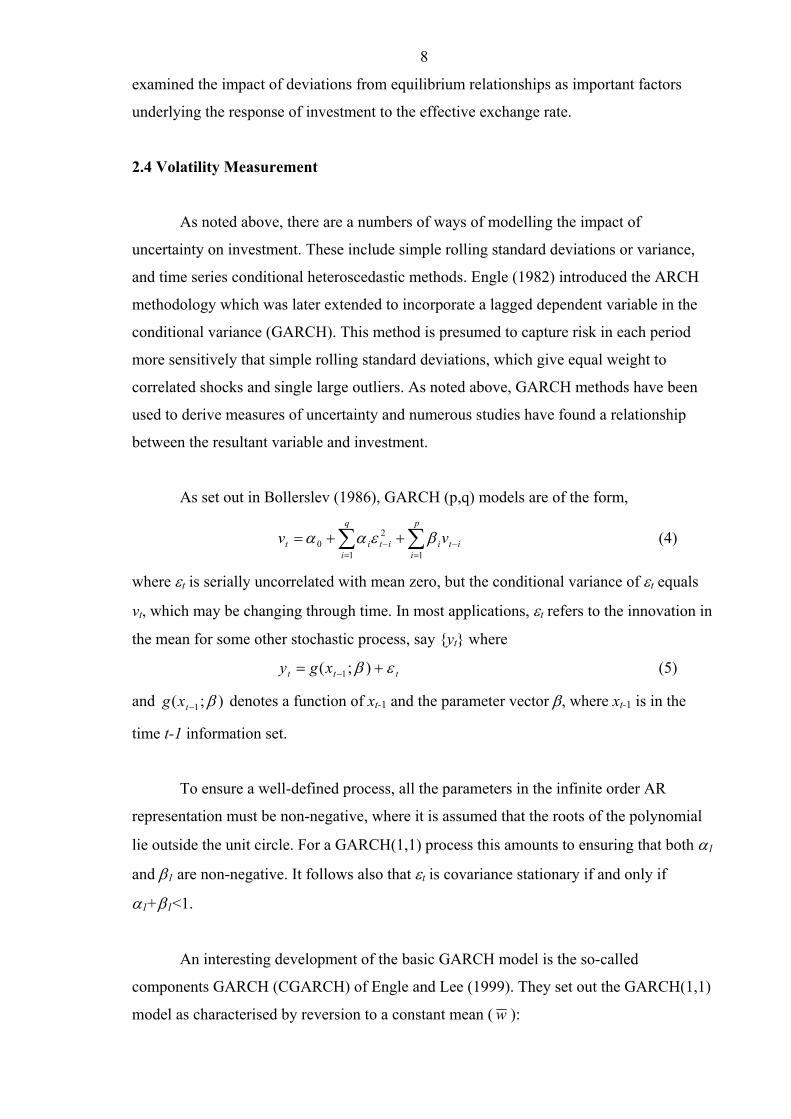
As set out in Bollerslev (1986), GARCH (p,q) models are of the form,

∑ ∑= =

−− ++=q

i

p

iitiitit vv

1 1

20 βεαα (4)

where εt is serially uncorrelated with mean zero, but the conditional variance of εt equals

vt, which may be changing through time. In most applications, εt refers to the innovation in

the mean for some other stochastic process, say {yt} where

ttt xgy εβ += − );( 1 (5)

and );( 1 β−txg denotes a function of xt-1 and the parameter vector β, where xt-1 is in the

time t-1 information set.

To ensure a well-defined process, all the parameters in the infinite order AR

representation must be non-negative, where it is assumed that the roots of the polynomial

lie outside the unit circle. For a GARCH(1,1) process this amounts to ensuring that both α1

and β1 are non-negative. It follows also that εt is covariance stationary if and only if

α1+β1<1.

An interesting development of the basic GARCH model is the so-called

components GARCH (CGARCH) of Engle and Lee (1999). They set out the GARCH(1,1)

model as characterised by reversion to a constant mean ( w ):

9

( ) ( )www ttt −+−+= −−2

112

112 σβεασ (6)

The components model allows reversion to a varying mean tq using an autoregressive term

ρ, modelled as

( ) ( )wwwq tttt −+−+=− −−2

112

112 σβεασ (7)

( ) ( )21

21010 −−− −+−+= tttt qq σεφαρα (8)

Equation (7) defines the temporary component ( tt q−2σ ), whilst equation (8) is the

permanent equation. When 0 < ( ) 111 <+ βα , short run volatility converges to its mean of 0,

while if 0 < ρ < 1 the long run component converges to its mean of α0 /(1- ρ). As the long

run volatility is more persistent than the short run, it is also assumed that 0 < (α1 + β1) < ρ

< 1. For negative variance to be ruled out, sufficient conditions are that α1, β1 and α0 are

positive and that β1 > φ > 0.

An objection to both GARCH and CGARCH is that they assume symmetry

between positive and negative shocks in terms of their effect on conditional volatility. For

example, it is plausible that a negative shock to exchange rates gives rise to higher

uncertainty as it could entail heightened expectations of a speculative attack.

The Exponential GARCH model was introduced by Nelson (1991) with the

following specification.

1

1

1

121

2 loglog−

−

−

−− +++=

t

t

t

ttt w

σε

γσε

ασβσ (9)

Hence the EGARCH describes the relationship between the past shocks and the log of the

conditional variance. Since it is specified in logs, no parameter restrictions have to be

imposed to ensure that the conditional variance is non-negative. Negative shocks have an

impact of α - γ on the log of the conditional variance and positive shocks have an effect of

α + γ. Hence there is an asymmetry if γ ≠ 0. For example, if γ < 0, 0 < α < 1 and α + β < 1,

negative shocks have a larger effect on conditional variance than positive shocks of the

same size.

2.5 Panel Estimation

The impact of uncertainty on investment is usefully captured in a cross-country

sample by using Pesaran, Shin and Smith’s (1999) Pooled Mean Group Estimator (PMGE)

10

for dynamic heterogeneous panel models. Panel methods have become popular in cross

sectional macro data sets, since they provide greater power that individual country studies

and hence greater efficiency.

Pesaran et al. emphasised that there are two traditional methods when estimating

panel models: averaging and pooling. The former involves running N separate regressions

and calculating coefficient means (see for example the Mean Group Estimator method

suggested by Pesaran and Smith, 1995). A drawback to averaging is that it does not

account for the fact that certain parameters may be equal over cross sections. Alternatively,

pooling the data typically assumes that the slope coefficients and error variances are

identical. This is unlikely to be valid for short-run dynamics and error variances, although

it could be appropriate for the long run.

Pesaran et al. (1999) proposed the PMGE method, which is an intermediate case

between the averaging and pooling methods of estimation, and involves aspects of both.

The PMGE method restricts the long-run coefficients to be equal over the cross-section,

but allows for the short-run coefficients and error variances to differ across groups on the

cross-section. We can therefore obtain pooled long-run coefficients and averaged short run

dynamics as an indication of mean reversion.

The PMGE is based on an Autoregressive Distributive Lag ARDL(p,q,…,q) model

∑∑=

−=

− ++′+=q

jitijitij

p

jjitijit yy

01

εµδλ x (10)

where itx (kx1) is the vector of explanatory variables for group i, µi represents the fixed

effects, the coefficients of the lagged dependent variables (λij) are scalars and δij are (kx1)

coefficient vectors. T must be large enough so that the model can be estimated for each

cross section.

Equation (10) can be re-parameterised as:

itijit

q

jij

p

jjitijitiitiit yyy εµδλβφ ++∆+∆+′+=∆ −

−

=

∗−

=−

∗− ∑∑ xx

1

0

1

11 ' (11)

where

−−= ∑ =

p

j iji 11 λφ , ∑ =

=q

j iji 0δβ , ∑ +=

∗ −=p

jm imij 1λλ and ∑ +=

∗ −=q

jm imij 1δδ

In addition, we assume that the residuals in (11) are i.i.d. with zero mean, variance greater

than zero and finite fourth moments. Secondly, the roots of equation (11) must lie outside

11

the unit circle. The latter assumption ensures that φi<0, and hence that there exist a long-

run relationship between yit and xit defined by

( ) ititiiity ηφβ +′−= x/ (12)

The long-run homogeneous coefficient is equal to ( )iii φβθθ /′−== , which is the same

across groups. The PMGE uses a maximum likelihood approach to estimate the model and

a Newton-Raphson algorithm. The lag length for the model can be determined using, for

instance, the Schwarz Bayesian Information Criteria. The estimated coefficients in the

model are not dependent upon whether the variables are I(1) or I(0). The key feature of the

PMGE is to make the long-run relationships homogenous while allowing for

heterogeneous dynamics and error variances.

2.6 Specification

Drawing on the insights provided in the discussion of Sections 2.1-2.5, we

estimated the impact of exchange rate uncertainty in a neoclassical investment function

which also allows in variants for the influence of Tobin's Q. Estimation was carried out

using Pooled-Mean-Group estimation with exchange-rate uncertainty proxies estimated by

CGARCH and EGARCH. As a baseline, we first set out the main result of Byrne and

Davis (2002) using a simple GARCH (1,1) approach. This was itself a considerable

advance on previous work for adopting the PMGE approach and testing for poolability. We

sought to further refine the approach to investment and exchange rate uncertainty, adopting

the insights of Chadha and Sarno (2002) by decomposing uncertainty into a permanent and

transitory component. However, our approach uses the Engle and Lee (1999) approach to

modelling GARCH, in contrast to the methods of Chadha and Sarno (2002) who utilise a

unobserved components model and maximum likelihood estimation to identify the

permanent and temporary aspects of price uncertainty. The authors also consider their

methods in terms of single equation estimation for each country, and we try to move

beyond this with panel estimation. Finally, we focus on exchange rate uncertainty, whereas

Chadha and Sarno look at price level uncertainty. Additionally we consider the point raised

by Baum et al. (2001) that there could be asymmetries from exchange rate uncertainty

depending on whether they link to an appreciation or depreciation. We do this by

employing the EGARCH approach of Nelson (1991), which allows for such asymmetries

in conditional volatility generation from positive and negative shocks.

12

In our estimation, besides using PMGE, we also calculated the Mean Group (MGE)

estimator, which is an average of the individual country coefficients. This provides

consistent estimates of the mean of the long-run coefficients, although they are inefficient

if slope homogeneity holds. Under long-run homogeneity, PMG estimates are consistent

and efficient. We test for long-run homogeneity using a joint Hausman test based on the

null of equivalence between the PMG and MG estimation (see Pesaran, Smith and Im,

1996, for details). If we reject the null (obtain a probability value of less that 0.05), we

reject homogeneity of our cross section’s long run coefficients. Significant statistical

difference between our two estimators would be indicative of panel misspecification.3 The

likelihood ratio test for long run parameter heterogeneity is much more conventional in this

setting and has homogeneity as the null hypothesis (see Hsiao, 1986).

3. Results

3.1 Data

The main source of data for the G7 countries is the OECD Business Sector

Database. A typical problem with private sector investment data is the distortion caused by

transfer of ownership e.g. in privatisations. Our quarterly OECD data set circumvents this

problem by incorporating business investment and output irrespective of ownership. Our

monthly effective exchange rate data is obtained from Primark Datastream. As shown in

Appendix A, all the macroeconomic variables, namely investment, output and Tobin’s Q

are non stationary according to Elliott, Rothemberg and Stock (1996) and Ng and Perron’s

(2001) feasible point optimal test and the modified point optimal test. The GARCH

outturns also were generally seen as non-stationary, albeit to an extent that depended upon

the lag length in the unit root tests as determined by the modified AIC tests. A similar

result was found by Ng and Perron (2001) for inflation. The non-stationary properties of

the data suggest an error correction approach to modelling investment is appropriate, so

long as cointegration is present.

3.2 GARCH estimation

The results for the CGARCH are presented in Table 1 below. It can be seen that the

transitory equations are fairly conventional, with significant positive ARCH terms of 0.07-

3 Pesaran and Smith (1995) illustrate that traditional approaches to estimation of pooled models (e.g. fixed effects, IV and generalised method of moments) produce potentially misleading coefficient estimates for

13

0.43. The GARCH terms in the transitory equations are more variable, with those for the

UK and Germany being insignificant and that for Japan being negative. Stability of short

run volatility is established (the sum of coefficients being between zero and one) except for

Japan. As regards the determinants of the long run component, there is a positive constant,

which is significant except for Italy, and a very large autoregressive component, implying

slow convergence of permanent volatility on its mean level. The size of the autoregressive

component exceeds that of the transitory components, implying slower mean reversion in

the long run. The component is below one in all cases, implying the process is stable.

Finally the permanent ARCH less GARCH term is significant except in the US and is

negative in Canada and France, positive elsewhere,

Table 1: Components GARCH estimate for nominal effective exchange rate UK US Germany Japan Canada France Italy Perm: Constant (α0)

0.00177 (0.295)

0.0004 (5.168)

0.0001 (10.148)

0.00118 (1.189)

0.000112 (9.427)

0.0000346 (4.465)

0.0041 (0.281)

Perm [q- α0] (ρ)

0.998 (969.623)

0.993 (740.677)

0.934 (28.330)

0.997 (513.209)

0.981 (257.540)

0.995 (6149.583)

0.998 (204.582)

perm [arch-garch] (φ)

0.043 (2.470)

-0.041 (0.997)

0.027 (0.793)

0.022 (12.595)

-0.053 (3.042

-0.027 (2.837)

0.243 (4.045)

Tran [arch-q] (α)

0.37 (6.076)

0.089 (1.954)

0.132 (2.396)

0.179 (3.709)

0.0973 (2.399)

0.339 (7.473)

0.334 (6.268)

Tran [garch-q] (β)

0.168 (1.239)

0.877 (22.878)

0.417 (1.597)

-0.27 (2.046)

0.725 (9.180)

-0.016 (0.138)

0.402 (4.536)

Notes: T-statistics are in parentheses. Bold indicates significance at 5%.

Table 2: Exponential GARCH estimate for nominal effective exchange rate UK US Germany Japan Canada France Italy Constant (w) -1.4

(6.505) -0.375 (6.249)

-2.7 (4.383)

-0.141 (252.989)

-0.75 (5.057)

-8.7 (4.511)

-2.77 (11.273)

Absolute (α) (res/garch)

0.485 (7.797)

0.06 (2.295)

0.354 (7.245)

-0.064 (9.253)

0.038 (0.763)

0.39 (6.295)

0.998 (24.614)

(res/garch) (γ) -0.064 (1.520)

-0.005 (0.290)

0.107 (3.070)

-0.057 (3.591)

-0.079 (2.369)

0.064 (1.225)

-0.0089 (0.230)

EGARCH (β) 0.875 (39.076)

0.96 (182.938)

0.74 (11.175)

0.974 (1636.8)

0.922 (69.3712)

0.086 (0.422)

0.775 (31.391)

Notes: T-statistics are in parentheses. Bold indicates significance at 5%

implying a possibility of negative volatility in those countries. The charts appended show

the estimated transitory and permanent components of volatility for the G7 countries.4

The results for the EGARCH are given in Table 2. We noted above that there are

no required constraints on signs for avoiding negative volatility, since the specification is

large T, unless cross section coefficients are identical.

14

set out in logs. In fact asymmetric effects are only significant in Germany, Japan and

Canada. In Japan and Canada it is negative shocks that give rise to heightened volatility

and in Germany it is appreciation (probably a reflection of ERM crises when the DM was

under upward pressure – and thus consistent with depreciation in the UK, France and

Italy).

3.3 Panel Estimation

We now go on to present the results of PMGE and MGE estimation. The

Likelihood Ratio (LR) test statistic and the Hausman test statistic (both distributed as χ2)

examine panel heterogeneity. The LR statistic always suggests that homogeneity is not a

reasonable assumption in the Pesaran et al. (1999) study of aggregate consumption and, as

such, can be considered a much more stringent test for poolability than the Hausman test

(which typically accepts poolability in the Pesaran et al. study). Accordingly, we focus

largely on the LR test in the following results.

As a baseline, Table 3 replicates the result of Byrne and Davis (2002) using

GARCH (1,1). Columns 1 and 2 show the results for PMG and MGE estimation of the

long run components of our basic investment function in the G7 with nominal exchange

rate uncertainty effects. We show estimated long run coefficients of business output,

ln(YB), the conditional variance of the nominal effective exchange rate, estimated error

correction terms, the Likelihood Ratio and Hausman statistics. In the equation, the long run

elasticity on output is significant and the estimated coefficient is slightly larger than one in

magnitude. Also, the error correction term is significant and gives evidence of mean

reversion to a long-run relationship and cointegration. The user cost was omitted as

insignificant. In terms of the measures of volatility, we find that the measure of nominal

exchange rate uncertainty is significant in influencing long-run business investment across

the G7 with a PMG estimated elasticity of –8.018. We see from the probability values

associated with the Hausman test of equivalence of PMG and MG that it accepts (p-value >

0.05) and hence, according to this test there is parameter homogeneity across the G-7 as a

whole. However, we cannot accept parameter homogeneity for the LR test for the G-7 (test

statistic χ2{12} = 30.72, whilst the critical value is 21.03). This suggests a need to focus on

4 The quarterly conditional volatility time series is based on the last month of each quarter. Alternative methods were tried and did not materially effect the results.

15

subgroups, and indeed as shown in columns 4 and 5, the EU-4 of the UK, France, Germany

and Italy do allow for pooling as well as having a significant exchange rate effect.

Table 3: PMG Estimation of Investment and Exchange Rate Uncertainty: G7 and EU4 Countries PMGE MGE PMGE MGE G7 EU4 Ln(YB) 1.346

(24.944) 1.439

(11.637) 1.233

(21.371) 1.202

(63.534) CV(DER) -8.018

(2.887) -25.198 (2.097)

-11.808 (3.312)

-12.670 (2.852)

Error Correction

-0.077 (5.270)

-0.083 (4.431)

-0.094 (3.855)

-0.097 (4.578)

Likelihood (Unrestricted)

1652.252 (1667.613)

935.335 (937.006)

LR Statistic χ2 {df}

30.72 {12} [p=0.00]

4.19 {6} [0.65]

Hausman χ2 {df}

3.44 {12} [0.18]

Na

Notes: Dependent variable Business Investment. PMGE is Pooled Mean Group Estimation. MGE is Mean Group Estimation. Sample period 1973Q1 to 1996Q4. T statistics are in parentheses. P-values are in square brackets. The lag structure is determined by the Schwarz Bayesian Criteria. The LR Statistic is a likelihood ratio test for the null hypothesis of poolability. Hausman test for poolability is a test for the equivalence of PMGE and MGE. If the null hypothesis is accepted (i.e. p-value greater than 0.05) we can accept homogeneity of cross sectional long run coefficients. CV(.) is the conditional variance from GARCH (1,1) estimation. DER is the log first difference of the nominal effective exchange rate.

Table 4: PMG Estimation of Investment and Exchange Rate Uncertainty: G7 Countries

PMGE MGE PMGE MGE PMGE MGE ln(YB) 1.347

(26.881) 1.240

(22.196) 1.359

(26.178) 2.347

(2.510) 1.333

(24.685) 1.339

(10.480) CV(PERM) 261.184

(1.378) 1334.829 (0.796)

679.584 (2.243)

1190.854 (0.647)

CV(TEMP) -150.574 (1.677)

-6383.884 (1.166)

-372.750 (2.627)

-759.049 (1.701)

Error Correction

-0.082 (5.946)

-0.082 (5.314)

-0.080 (5.840)

-0.082 (4.23)

-0.079 (4.808)

-0.079 (4.197)

Likelihood (Unrestricted)

1653.899 (1669.610)

1652.139 (1670.381)

1652.565 (1675.343)

LR Statistic χ2 {df}

31.442 [0.002]

36.484 [0.000]

38.424 [0.003]

Hausman Test χ2 {df}

Na 3.35 [0.19]

25.04 [0.00]

Notes: See Table 3, also CV (PERM) represents permanent component from CGARCH, CV (TEMP) the corresponding transitory component. These results are for the G7: the US, Canada, Japan, Italy, France, Germany and the UK. Sample period 1973Q1 to 1996Q4.

Table 4 shows the results in the G7 of the estimation of separate components of the

CGARCH separately and together.5 The results show that neither transitory nor permanent

volatility entered separately has a significant effect on investment, although there is some

evidence of a negative effect from the transitory component at the 10% significance level.

5 The stationarity properties of the data are considered in appendix A. Typically all variables are I(1) and the small amount of evidence of stationarity is not unexpected give the large number of tests we conduct.

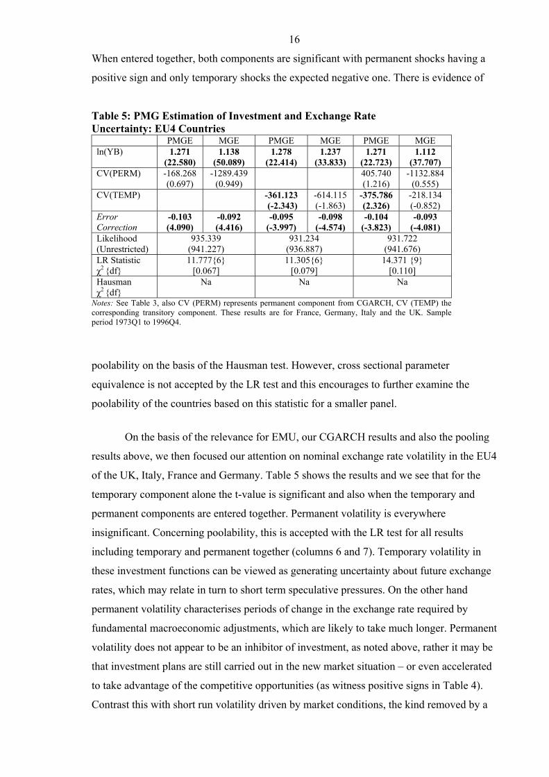
16

When entered together, both components are significant with permanent shocks having a

positive sign and only temporary shocks the expected negative one. There is evidence of

Table 5: PMG Estimation of Investment and Exchange Rate Uncertainty: EU4 Countries

PMGE MGE PMGE MGE PMGE MGE ln(YB) 1.271

(22.580) 1.138

(50.089) 1.278

(22.414) 1.237

(33.833) 1.271

(22.723) 1.112

(37.707) CV(PERM) -168.268

(0.697) -1289.439

(0.949) 405.740

(1.216) -1132.884

(0.555) CV(TEMP) -361.123

(-2.343) -614.115 (-1.863)

-375.786 (2.326)

-218.134 (-0.852)

Error Correction

-0.103 (4.090)

-0.092 (4.416)

-0.095 (-3.997)

-0.098 (-4.574)

-0.104 (-3.823)

-0.093 (-4.081)

Likelihood (Unrestricted)

935.339 (941.227)

931.234 (936.887)

931.722 (941.676)

LR Statistic χ2 {df}

11.777{6} [0.067]

11.305{6} [0.079]

14.371 {9} [0.110]

Hausman χ2 {df}

Na Na Na

Notes: See Table 3, also CV (PERM) represents permanent component from CGARCH, CV (TEMP) the corresponding transitory component. These results are for France, Germany, Italy and the UK. Sample period 1973Q1 to 1996Q4.

poolability on the basis of the Hausman test. However, cross sectional parameter

equivalence is not accepted by the LR test and this encourages to further examine the

poolability of the countries based on this statistic for a smaller panel.

On the basis of the relevance for EMU, our CGARCH results and also the pooling

results above, we then focused our attention on nominal exchange rate volatility in the EU4

of the UK, Italy, France and Germany. Table 5 shows the results and we see that for the

temporary component alone the t-value is significant and also when the temporary and

permanent components are entered together. Permanent volatility is everywhere

insignificant. Concerning poolability, this is accepted with the LR test for all results

including temporary and permanent together (columns 6 and 7). Temporary volatility in

these investment functions can be viewed as generating uncertainty about future exchange

rates, which may relate in turn to short term speculative pressures. On the other hand

permanent volatility characterises periods of change in the exchange rate required by

fundamental macroeconomic adjustments, which are likely to take much longer. Permanent

volatility does not appear to be an inhibitor of investment, as noted above, rather it may be

that investment plans are still carried out in the new market situation – or even accelerated

to take advantage of the competitive opportunities (as witness positive signs in Table 4).

Contrast this with short run volatility driven by market conditions, the kind removed by a

17

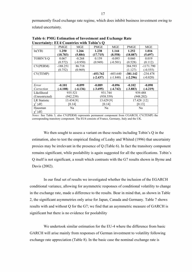
permanently fixed exchange rate regime, which does inhibit business investment owing to

related uncertainty.

Table 6: PMG Estimation of Investment and Exchange Rate Uncertainty: EU4 Countries with Tobin’s Q

PMGE MGE PMGE MGE PMGE MGE ln(YB) 1.250

(18.783) 1.266

(5.884) 1.238

(17.715) 1.144

(8.558) 1.252

(18.887) 1.016

(5.697) TOBIN’S Q 0.067

(0.572) -0.268

(-0.950) 0.159

(0.949) -0.093

(-0.501) 0.060

(0.528) 0.019

(0.112) CV(PERM) -188.251

(0.752) 86.718 (0.969)

384.593 (1.127)

-1171.790 (-0.555)

CV(TEMP) -453.762 (-2.437)

-603.640 (-1.848)

-381.142 (-2.296)

-234.478 (-0.820)

Error Correction

-0.101 (-4.108)

-0.099 (-4.136)

-0.089 (-3.695)

-0.096 (-4.742)

-0.102 (-3.883)

-0.090 (-4.219)

Likelihood (Unrestricted)

935.521 (942.239)

931.744 (938.559)

939.488 (948.202)

LR Statistic χ2 {df}

13.434{9} [0.14]

13.629{9} [0.14]

17.428 {12} [0.13]

Hausman χ2 {df}

Na Na Na

Notes: See Table 3, also CV(PERM) represents permanent component from CGARCH, CV(TEMP) the corresponding transitory component. The EU4 consists of France, Germany, Italy and the UK.

We then sought to assess a variant on these results including Tobin’s Q in the

estimation, also to test the empirical finding of Leahy and Whited (1996) that uncertainty

proxies may be irrelevant in the presence of Q (Table 6). In fact the transitory component

remains significant, while poolability is again suggested for all the specifications. Tobin’s

Q itself is not significant, a result which contrasts with the G7 results shown in Byrne and

Davis (2002).

In our final set of results we investigated whether the inclusion of the EGARCH

conditional variance, allowing for asymmetric responses of conditional volatility to change

in the exchange rate, made a difference to the results. Bear in mind that, as shown in Table

2, the significant asymmetries only arise for Japan, Canada and Germany. Table 7 shows

results with and without Q for the G7; we find that an asymmetric measure of GARCH is

significant but there is no evidence for poolability

We undertook similar estimation for the EU-4 where the difference from basic

GARCH will arise mainly from responses of German investment to volatility following

exchange rate appreciation (Table 8). In the basic case the nominal exchange rate is

18

significant but poolability is not indicated. However, when Tobin’s q is added we also

accept poolability.

Table 7: Panel Estimation of Investment and Uncertainty: G7 Countries EGARCH

PMGE MGE PMGE MGE Ln(YB) 1.465

(21.859) 1.239

(6.224) 1.310

(22.864) 0.962

(3.722) TOBIN'S Q 0.265

(2.998) 0.616

(1.295) CV(DER) -280.845

(-2.484) -131.376 (-0.104)

-307.296 (-2.771)

216.84 (0.144)

Error Correction

-0.069 (-5.979)

-0.076 (-3.434)

-0.074 (-5.229)

-0.081 (-3.558)

Likelihood (Unrestricted)

1646.136 (1667.913)

1649.387 (1679.189)

LR Statistic χ2 {df}

43.555 {12} [0.00]

59.604{18} [0.00]

Hausman χ2 {df}

7.86 {12} [0.02]

18.30 {18} [0.00]

Notes: Dependent variable Business Investment. PMGE is Pooled Mean Group Estimation. MGE is Mean Group Estimation. Sample period 1973Q1 to 1996Q4. T statistics are in parentheses. P-values are in brackets. The lag structure is determined by the Schwarz Bayesian Criteria. The LR Statistic is a likelihood ratio test for the null hypothesis of poolability. Hausman test for poolability is a test for the equivalence of PMGE and MGE. If the null hypothesis is accepted (i.e. p-value greater than 0.05) we can accept homogeneity of cross sectional long run coefficients. CV(.) is the conditional variance from EGARCH estimation. DER is the first difference of the nominal effective exchange rate.

Table 8 Panel Estimation of Investment and Uncertainty: EU4 Countries EGARCH

PMGE MGE PMGE MGE Ln(YB) 1.273

(23.296) 1.216

(25.579) 1.188

(15.552) 1.091

(7.547) TOBIN'S Q 0.262

(1.193) -0.034

(-0.195) ECV(DER) -294.348

(-2.213) -1070.079 (-1.574)

-644.395 (-2.287)

-1096.323 (-1.605)

Error Correction

-0.097 (-3.582)

-0.096 (-4.395)

-0.078 (-2.808)

-0.092 (-4.685)

Likelihood (Unrestricted)

931.898 (938.482)

932.046 (940.417)

LR Statistic χ2 {df}

13.168{6} [0.040]

16.743 {9} [0.053]

Hausman χ2

Na Na

Notes: Dependent variable Business Investment. PMGE is Pooled Mean Group Estimation. MGE is Mean Group Estimation. Sample period 1973Q1 to 1996Q4. T statistics are in parentheses. P-values are in brackets. The LR Statistic is a likelihood ratio test for the null hypothesis of poolability. Hausman test for poolability is a test for the equivalence of PMGE and MGE. ECV(.) is the conditional variance from EGARCH estimation. DER is the first difference of the nominal effective exchange rate. EU4 represents France, Germany, Italy and the UK.

19

4. Conclusion

In this paper we have sought to shed light on the importance of exchange rate uncertainty

for business investment at a macroeconomic level. In particular, we have estimated the

impact on investment of temporary and permanent components of exchange rate

uncertainty derived using a components GARCH model. Additionally we have considered

asymmetric responses to exchange rate changes using an EGARCH. The key result is that

for a poolable subsample of EU countries, it is the transitory and not the permanent

component which adversely affects investment. This is consistent with an adaptation of the

suggestion in Baum et al. (2001) regarding profitability, namely, that permanent volatility

will not hinder investment as firms act to take advantage of related permanent shifts in the

exchange rate - while a rise in temporary volatility will dampen investment as firms

become more conservative under heightened uncertainty and delay their investment. Or,

following Moore and Schaller (2002), the different impact of persistent and temporary

economic shocks on investment decisions may be due to the evolution of beliefs under

learning.

The results imply that to the extent that EMU favours lower transitory exchange

rate volatility, it will also be beneficial to investment. EMU after all eliminates short run

volatility among the component currencies, linked inter alia to currency speculation, that

was rife in the ERM. Equally, there is some support for asymmetries in response of

uncertainty to shocks in Germany, Japan and Canada, and the results for investment

functions suggest that the conditional variances derived are successful in an investment

function specification for the EU-4 including Tobin’s Q.

20

References

Abel, A. (1980) Empirical investment equations: An integrated framework. Carnegie Rochester

Conference Series on Public Policy 12, 39-91.

Abel, A. (1983) Optimal investment under uncertainty. American Economic Review 73, 228-233.

Ashworth, P.D. and Davis, E.P. (2001) Some evidence on financial factors in the determination of

aggregate business investment for the G7 countries. NIESR Discussion Paper #187.

Ball, L., Cecchetti, S. (1990) Inflation and uncertainty at short and long Horizons. Brookings Paper

on Economic Activity 215-54.

Baum, C. F., Caglayan, M., Barkoulas, J.T. (2001) Exchange Rate Uncertainty and Firm

Profitability. Journal of Macroeconomics 23, 565-76.

Bean, C. (1981) An econometric model of manufacturing investment in UK manufacturing.

Economic Journal, 91, 106-121.

Beveridge S and Nelson C R (1981), “New approach to decomposition of economic time series into

permanent and transitory components with particular attention to measurement of the “Business

Cycle””, Journal of Monetary Economics, 7, 151-174

Byrne, J.P., Davis, E.P. (2002) Investment and Uncertainty in the G7. NIESR Discussion Paper

199.

Bollerslev, T. (1990) Modelling the coherence in short run nominal exchange rates: A multivariate

generalised ARCH model, Review of Economics and Statistics 72, 498-505.

Callen, T.S., Hall S.G., and S G B Henry (1990), Manufacturing stocks, expectations, risk and

cointegration, Economic Journal, 100, 756-772

Carruth A., Dickerson A., Henley, A. (2000b) What do we know about investment under

uncertainty? Journal of Economic Surveys 14, 119-153.

Chadha, J.S. and Sarno, L. (2002) Short- and long-run price level uncertainty under different

monetary policy regimes: An international comparison. Oxford Bulletin of Economics and Statistics

64, 183-212.

Cuthbertson, K. and Gasparro (1995) Fixed investment decision in UK manufacturing: The

importance of Tobin's Q, output and debt. European Economic Review 39, 919-941.

Darby, J. Hughes Hallett, A. Ireland, J. and Piscatelli, L. (1999) The impact of exchange rate

uncertainty on the level of investment. Economic Journal 109, C55-C67.

Darby, J., Hughes Hallett, A., Ireland, J., Piscatelli, L. (2002) Exchange rate uncertainty, price

misalignments and business sector investment. University of Strathclyde, mimeo.

Dixit, A., Pindyck, R.S. (1994) Investment under Uncertainty. Princeton University Press.

21

Driver, C., Moreton, D. (1991) The influence of uncertainty on aggregate spending. Economic

Journal 101, 1452-59.

Elliott, G., Rothemberg, T.J. and Stock, J.H. (1996) Efficient tests for an autoregressive unit root.

Econometrica 64, 813-836.

Engle, R.F. (1982) Autoregressive Conditional Heteroscedasticity with estimates of the variance of

UK inflation. Econometrica 50, 987-1008.

Engle, R.F., Lee, G.J. (1999) A Long Run and Short Run Component Model of Stock Return

Volatility. In Engle, R.F. and White, H. (eds.) Cointegration, Causality and forecasting: a

Festschrift in honour of Clive W.J. Granger.

Episcopes, A. (1995) Evidence on the relationship between uncertainty and aggregate investment.

Quarterly Journal of Economics and Finance 35, 41-52.

Goldberg, L.S. (1993) Exchange rates and investment in United States industry. Review of

Economics and Statistics 75, 575-589.

Hartman, R. (1972) The effect of price and cost uncertainty on investment. Journal of Economic

Theory 5, 258-266.

Hayashi, F. (1982) Tobin’s marginal Q and average Q: A neo-classical interpretation.

Econometrica 50, 213-24.

Huizinga, H. (1993) Inflation uncertainty, relative price uncertainty and investment in US

manufacturing. Journal of Money, Credit and Banking 25, 521-554.

Jorgenson, D.W. (1963) Capital theory and investment behaviour. American Economic Review 53,

247-259.

Kenen, P., Rodrick, D. (1986) Measuring and Analysing the effect of short term volatility in

exchange rates. Review of Economics and Statistics LXVIII, 311-319.

Lee, J., Shin, K. (2001) The role of variable input in the relationship between investment and

uncertainty. American Economic Review 90, 667-680.

Leahy, J., Whited, T. (1996) The effects of uncertainty on investment: Some stylised facts. Journal

of Money, Credit and Banking 28, 64-83.

Moore, B. and Schaller, L. (2002) Persistent and transitory shocks, learning, and investment

dynamics. Journal of Money, Credit and Banking 34(3), 650-677.

Nelson, D.B. (1991) Conditional heteroscedasticity in asset returns; a new approach. Econometrica

59, 347-70.

Ng, S., Perron, P. (2001) Lag Length Selection and the Construction of Unit Root Tests with Good

Size and Power. Econometrica 69(6), 1519-54.

22

Nucci, F., Pozzolo, A.F. (2001) Investment and the exchange rate: An analysis with firm-level

panel data. European Economic Review 45, 259-83.

Pagan, A., Ullah, A. (1988) The econometric analysis of models with risk terms. Journal of

Applied Econometrics 3, 87-106.

Pesaran, M.H., Shin, Y., Smith, R. (1999) Pooled Mean Group estimation of dynamic

heterogeneous panels. Journal of the American Statistical Association 94, 621-634.

Pesaran, M.H., Smith, R. (1995) Estimating long-run relationships from dynamic heterogeneous

panels. Journal of Econometrics 68, 79-113.

Pesaran, M.H., Smith, R., Im, K-S. (1996) Dynamic linear models for heterogeneous panels. In L.

Matyas and P. Sevestre (eds.) The Econometrics of Panel Data, Kluwer Academic Publishers.

Price, S. (1995) Aggregate uncertainty, capacity utilization and manufacturing investment. Applied

Economics 27, 147-154.

Sensenbrenner, G. (1991) Aggregate investment, the stock market, and the Q model - robust results

for six OECD countries. European Economic Review 35, 769-825.

Serven, L. (2003) Real exchange rate uncertainty and private investment in developing countries,

forthcoming, Review of Economics and Statistics

Tobin, J. (1969) A general equilibrium approach to monetary theory. Journal of Money, Credit and

Banking 1, 15-29.

23

Table A1 Unit Root Tests Components GARCH Permanent and Temporary Conditional Volatility US CA FR GE IT JP UK

Ln(IB) k 1 2 0 0 2 2 0 (trend) AR(α): 0.925 0.943 0.965 0.964 0.923 0.961 0.947 ERS Pt 6.534 9.921 30.981 34.608 7.761 9.39 20.619 M Pt 6.592 8.869 28.389 28.895 7.84 8.472 18.854 Ln(YB) k 1 1 2 0 1 3 3 (trend) AR(α): 0.919 0.945 0.942 0.97 0.946 0.942 0.963 ERS Pt 8.528 9.917 9.347 35.442 11.009 8.764 15.751 M Pt 7.83 9.341 8.855 32.837 9.31 8.28 12.957 Tobin’s Q k 0 4 6 2 1 4 2 (trend) AR(α): 0.99 0.948 0.98 0.988 0.917 0.97 0.955 ERS Pt 65.784 10.809 64.417 40.762 8.448 16.945 27.892 M Pt 51.038 9.075 54.514 35.741 8.623 16.063 21.385 Ln(IB) k 1 1 2 0 1 3 3 (constant) AR(α): 0.919 0.945 0.942 0.97 0.946 0.942 0.963 ERS Pt 8.528 9.917 9.347 35.442 11.009 8.764 15.751 M Pt 7.83 9.341 8.855 32.837 9.31 8.28 12.957 Ln(YB) k 9 3 12 4 11 4 4 (constant) AR(α): 1.003 1.005 1.002 1.006 1.001 1.001 1.005 ERS Pt 36.351 114.525 72.892 67.288 38.025 27.053 56.244 M Pt 28.302 84.843 54.207 53.91 27.687 20.927 46.814 Tobin’s Q k 0 4 11 2 7 4 2 (constant) AR(α): 0.992 0.963 1.008 0.983 0.972 0.974 0.983 ERS Pt 25.957 3.824 35.481 17.76 11.129 5.229 12.373 M Pt 22.201 3.707 31.705 14.904 9.732 5.311 12.544 Notes: K is the lag length determined by the Modified AIC, see Ng and Perron (2001). Sample period 1973Q1 1996Q4. AR(α) is the estimated autoregressive coefficient. All variables have been detrended by GLS for both the statistic and spectral density. Estimated statistics in bold indicate stationarity. ERS Pt is the Elliott, Rothemberg and Stock (1996) feasible point optimal test. M Pt is the modified point optimal test. 5% critical value is 5.48 for case with trend. 5% Critical Value is 3.17 with constant. Test statistics of less than the critical value reject the null hypothesis of unit root.

24

Table A2 Unit Root Tests Components GARCH Permanent and Temporary Conditional Volatility -Trend

US CA FR GE IT JP UK CV(NEER) k 6 7 1 5 11 0 1 (trend) AR(α): 0.911 0.610 0.915 0.722 0.491 0.931 0.785 Permanent ERS Pt 141.630 36.435 18.543 23.263 12.889 15.173 6.995 M Pt 107.410 33.669 15.791 23.591 12.922 14.636 6.484 CV(NEER) k 5 5 12 9 9 6 4 (trend) AR(α): 0.879 0.602 0.793 0.499 0.615 0.845 0.282 Temporary ERS Pt 17.533 8.608 192.901 122.701 17.597 84.182 4.077 M Pt 17.845 8.774 175.514 123.644 17.945 66.216 4.142 CV(NEER) k 1 4 5 9 9 6 3 (trend) AR(α): 0.884 0.796 0.817 0.615 0.607 0.791 0.330 total ERS Pt 9.805 9.849 41.548 137.853 15.413 48.247 4.168 M Pt 9.671 9.974 35.877 139.030 15.657 40.864 4.248 Notes: K is the lag length determined by the Modified AIC see Ng and Perron (2001). Sample period 1973Q1 1996Q4. Alpha-hat is the estimated autoregressive coefficient. All variables have been detrended by GLS for both the statistic and spectral density. Estimated statistics in bold indicate stationarity. ERS Pt is the Elliott, Rothemberg and Stock (1996) feasible point optimal test. M Pt is the modified point optimal test. 5% Critical Value 5.48. Test statistics of less than the critical value reject the null hypothesis of unit root. Table A3 Unit Root Tests Components GARCH Permanent and Temporary Conditional Volatility -Constant

US CA FR GE IT JP UK CV(NEER) k 6 7 1 5 11 0 1 (constant) AR(α): 1.010 0.908 1.008 0.914 0.770 0.998 0.934 Permanent ERS Pt 179.375 25.143 86.098 12.380 13.303 37.104 8.263 M Pt 118.162 24.986 60.577 11.372 12.063 27.166 5.988 CV(NEER) k 5 5 5 9 9 6 1 (constant) AR(α): 0.880 0.946 0.946 0.807 0.684 0.989 0.147 Temporary ERS Pt 4.970 18.278 31.476 62.383 6.848 104.892 0.995 M Pt 5.048 14.880 23.069 62.773 6.754 70.210 0.988 CV(NEER) k 1 4 5 7 9 5 3 (constant) AR(α): 0.922 0.988 1.012 0.779 0.724 0.871 0.336 Total ERS Pt 4.308 27.154 77.956 14.608 7.601 18.788 1.921 M Pt 3.739 22.276 53.960 14.502 7.282 14.666 1.801 Notes: K is the lag length determined by the Modified AIC see Ng and Perron (2001). Sample period 1973Q1 1996Q4. Alpha-hat is the estimated autoregressive coefficient. All variables have been detrended by GLS for both the statistic and spectral density. Estimated statistics in bold indicate stationarity. ERS Pt is the Elliott, Rothemberg and Stock (1996) feasible point optimal test. M Pt is the modified point optimal test. 5% Critical Value 3.17. Test statistics of less than the critical value reject the null hypothesis of unit root.

25

Table A4 Unit Root Tests : Asymmetric GARCH (EGARCH) US CA FR GE IT JP UK

ECV(NEER) k 0 2 10 11 9 0 0 (trend) AR(α): 0.965 0.834 0.906 0.615 0.739 0.881 0.460 ERS Pt 27.705 9.862 235.484 197.344 31.808 9.854 2.465 M Pt 24.090 9.262 181.575 199.943 32.026 8.749 2.511 ECV(NEER) k 0 2 11 10 9 0 0 (constant) AR(α): 0.984 0.950 1.015 0.851 0.886 0.980 0.455 ERS Pt 25.054 9.626 967.020 60.855 19.584 16.060 0.705 M Pt 17.832 7.204 640.281 59.440 17.617 11.268 0.710 Notes: K is the lag length determined by the Modified AIC see Ng and Perron (2001). Sample period 1973Q1 1996Q4. Alpha-hat is the estimated autoregressive coefficient. All variables have been detrended by GLS for both the statistic and spectral density. Estimated statistics in bold indicate stationarity. ERS Pt is the Elliott, Rothemberg and Stock (1996) feasible point optimal test. M Pt is the modified point optimal test. 5% critical value is 5.48 for case with trend. 5% Critical Value is 3.17 with constant. Test statistics of less than the critical value reject the null hypothesis of unit root.

26

Figure B1 Total (CGVAR), Transitory (CGMQ) and Permanent component measures of volatility for G7 Key UK: United Kingdom; DE: Germany; IT: Italy; FR: France.

-0.0002

0

0.0002

0.0004

0.0006

0.0008

0.001

0.001219

73Q

119

74Q

2

1975

Q3

1976

Q4

1978

Q1

1979

Q2

1980

Q3

1981

Q4

1983

Q1

1984

Q2

1985

Q3

1986

Q4

1988

Q1

1989

Q2

1990

Q3

1991

Q4

1993

Q1

1994

Q2

1995

Q3

1996

Q4

CGVARUK QUK CGMQUK

-0.0001

0

0.0001

0.0002

0.0003

0.0004

0.0005

0.0006

1973

Q1

1974

Q2

1975

Q3

1976

Q4

1978

Q1

1979

Q2

1980

Q3

1981

Q4

1983

Q1

1984

Q2

1985

Q3

1986

Q4

1988

Q1

1989

Q2

1990

Q3

1991

Q4

1993

Q1

1994

Q2

1995

Q3

1996

Q4

CGVARDE QGE CGMQGE

-0.0001

0

0.0001

0.0002

0.0003

0.0004

0.0005

0.0006

1973

Q1

1974

Q2

1975

Q3

1976

Q4

1978

Q1

1979

Q2

1980

Q3

1981

Q4

1983

Q1

1984

Q2

1985

Q3

1986

Q4

1988

Q1

1989

Q2

1990

Q3

1991

Q4

1993

Q1

1994

Q2

1995

Q3

1996

Q4

CGVARFR QFR CGMQFR

-0.00050

0.00050.001

0.00150.002

0.00250.003

0.00350.004

0.0045

1973

Q1

1974

Q2

1975

Q3

1976

Q4

1978

Q1

1979

Q2

1980

Q3

1981

Q4

1983

Q1

1984

Q2

1985

Q3

1986

Q4

1988

Q1

1989

Q2

1990

Q3

1991

Q4

1993

Q1

1994

Q2

1995

Q3

1996

Q4

CGVARIT QIT CGMQIT

27

Figure B2: Total (CGVAR), Transitory (CGMQ) and Permanent (Q) component measures of volatility for G7 Key JP: Japan; CA: Canada; US: United States

-0.0002

-0.0001

0

0.0001

0.0002

0.0003

0.0004

0.000519

73Q

119

74Q

219

75Q

319

76Q

419

78Q

119

79Q

219

80Q

319

81Q

419

83Q

119

84Q

219

85Q

319

86Q

419

88Q

119

89Q

219

90Q

319

91Q

419

93Q

119

94Q

219

95Q

319

96Q

4

CGVARUS QUS CGMQUS

-0.0004-0.0002

00.00020.00040.00060.00080.001

0.00120.00140.0016

1973

Q1

1974

Q2

1975

Q3

1976

Q4

1978

Q1

1979

Q2

1980

Q3

1981

Q4

1983

Q1

1984

Q2

1985

Q3

1986

Q4

1988

Q1

1989

Q2

1990

Q3

1991

Q4

1993

Q1

1994

Q2

1995

Q3

1996

Q4

CGVARJP QJP CGMQJP

-0.0001

-0.00005

0

0.00005

0.0001

0.00015

0.0002

1973

Q1

1974

Q2

1975

Q3

1976

Q4

1978

Q1

1979

Q2

1980

Q3

1981

Q4

1983

Q1

1984

Q2

1985

Q3

1986

Q4

1988

Q1

1989

Q2

1990

Q3

1991

Q4

1993

Q1

1994

Q2

1995

Q3

1996

Q4

CGVARCA QCA CGMQCA

28

Figure B3. Exponential GARCH conditional volatility

0

0.0002

0.0004

0.0006

0.0008

0.001

73017502770379048201840286038804910193029503

0

0.001

0.002

0.003

0.004

0.005

US E G V A R CA E G V A R JP E G V A R ITE G V A R

00.00020.00040.00060.0008

0.0010.0012

730175017701790181018301850187018901910193019501

FREGVAR DEEGVAR UKEGVAR

JP: Japan; CA: Canada; US: United States UK: United Kingdom; DE: Germany; FR: France; IT: Italy (second y-axis)