Panel Data and Unobservable Individual EffectsAuthor(s): Jerry A. Hausman and William E. TaylorReviewed work(s):Source: Econometrica, Vol. 49, No. 6 (Nov., 1981), pp. 1377-1398Published by: The Econometric SocietyStable URL: http://www.jstor.org/stable/1911406 .Accessed: 19/04/2012 17:04

Your use of the JSTOR archive indicates your acceptance of the Terms & Conditions of Use, available at .http://www.jstor.org/page/info/about/policies/terms.jsp

JSTOR is a not-for-profit service that helps scholars, researchers, and students discover, use, and build upon a wide range ofcontent in a trusted digital archive. We use information technology and tools to increase productivity and facilitate new formsof scholarship. For more information about JSTOR, please contact support@jstor.org.

The Econometric Society is collaborating with JSTOR to digitize, preserve and extend access to Econometrica.

http://www.jstor.org

Econometrica, Vol. 49, No. 6 (November, 1981)

PANEL DATA AND UNOBSERVABLE INDIVIDUAL EFFECTS'

BY JERRY A. HAUSMAN AND WILLIAM E. TAYLOR2

An important purpose in combining time-series and cross-section data is to control for individual-specific unobservable effects which may be correlated with other explanatory variables. Using exogeneity restrictions and the time-invariant characteristic of the latent variable, we derive (i) a test for the presence of this effect and for the over-identifying restrictions we use, (ii) necessary and sufficient conditions for identification, and (iii) the asymptotically efficient instrumental variables estimator and conditions under which it differs from the within-groups estimator. We calculate efficient estimates of a wage equation from the Michigan income dynamics data which indicate substantial differences from within-groups or Balestra-Nerlove estimates-particularly, a significantly higher estimate of the returns to schooling.

1. INTRODUCTION

AN IMPORTANT BENEFIT from pooling time-series and cross-section data is the ability to control for individual-specific effects-possibly unobservable-which may be correlated with other included variables in the specification of an economic relationship. Analysis of cross-section data alone can neither identify nor control for such individual effects. To consider a specific model, let

(1.) Yit = X.,/

+ Z,y + a.

+ 7i (i = 1. * * N; t = 1,. ..,T)

where : and -y are k and g vectors of coefficients associated with time-varying and time-invariant observable variables respectively. The disturbance Nit is as- sumed uncorrelated with the columns of (X, Z, a) and has zero mean and constant variance a2 conditional on Xi, and Z,. The latent individual effect a,. is assumed to be a time-invariant random variable, distributed independently across individuals, with variance a,.

Our primary focus is the potential correlation of al, with the columns of X and Z. In the presence of such correlations, least squares (OLS) and generalized least squares (GLS) yield biased and inconsistent estimates of the parameters (/-y, Ca2), . The traditional technique to overcome this problem is to eliminate the individual effects in the sample by transforming the data into deviations from individual means.3 Unfortunately, the OLS coefficient estimates from the trans- formed data (known as "within-groups" or "fixed effects" estimators) have two important defects: (1) all time-invariant variables are eliminated by the transfor- mation, so that -y cannot be estimated, and (2) under certain circumstances, the within-groups estimator is not fully efficient since it ignores variation across

'Early versions of this paper were presented at the Econometric Society Summer Meetings in Montreal and at the Fourth World Congress in Aix en Provence.

2Hausman thanks the NSF for financial support. Rob Engle and Paul Ruud have given useful comments.

3This technique corresponds to Model I of the analysis of variance, e.g., Scheffe [19]. When used in analysis of covariance, errors in measured variables can create a serious problem since they are exacerbated by the data transformation.

1377

1378 J. A. HAUSMAN AND W. E. TAYLOR

individuals in the sample. The first problem is generally the more serious since in some applications, primary interest is attached to the unknown coefficients of the time-invariant variables, e.g., to the coefficients of schooling in the wage equa- tion below.

Another possible approach in the simultaneous equations model is to find instruments for those columns of X and Z which are potentially correlated with ai. However, it may be difficult to find appropriate instruments, excluded from equation (1.1), which are uncorrelated with ai, and, in any case, such procedures ignore the time-invariant characteristic of the latent effect.

Specifications similar to equation (1.1) have been used in at least two empirical contexts. In the cost and production function literature where ai denotes the managerial efficiency of the ith firm, Hoch [9] and Mundlak [14] have suggested the use of the within-groups estimator to produce unbiased estimates of the remaining parameters. If Yi, denotes the wages of the ith individual in the tth time period, one of the Zi's measures his schooling, and ai denotes his unmeasur- able ability or ambition, then equation (1.1) represents a standard specification for measuring the returns to education. To the extent that ability and schooling are correlated, the OLS estimates are biased and inconsistent. Griliches [4] has relied on an instrumental variables approach, using family background variables excluded from equation (1.1) as instruments.4 Another approach is the factor analytic model, pioneered in this context by Joreskog [10] and applied to the schooling problem by Chamberlain and Griliches [2] and Chamberlain [1]. This model relies for identification upon orthogonality assumptions imposed upon observable and unobservable components of ai. The method we propose does not assume a specification of the components of ai and may be less sensitive to our lack of knowledge about the unobservable individual-specific effect.

Instead, our method uses assumptions about the correlations between the columns of (X, Z) and ai . If we are willing to assume that certain variables among the X and Z are uncorrelated with ai, then conditions may hold such that all of the /B's and -y's may be consistently and efficiently estimated. Intuitively, the columns of Xi, which are uncorrelated with ai can serve two functions because of their variation across both individuals and time: (i) using deviations from individual means, they produce unbiased estimates of the /3's, and (ii) using the individual means, they provide valid instruments for the columns of Zi that are correlated with ai.

One needs to be quite careful in choosing among the columns of X for those variables which are uncorrelated with ai. For instance, in the returns to schooling example, it may be safe to assume that ability is uncorrelated with health or age but less so with unemployment. An important feature of our method is that, in certain circumstances, the non-correlation assumptions can be tested, so that the method need not rely on totally a priori assumptions.

4A specification test developed below suggests that, in our sample, family background is likely to be correlated with the latent individual effect.

PANEL DATA 1379

The plan of the paper is as follows. In Section 2, we formally set up the model and consider the standard estimation procedures. Using these procedures, we develop and compare three specification tests for correlation between a, and the columns of X and Z, generalizing results of Hausman [6]. In the event of such correlation, we propose a consistent but inefficient estimator of all the parame- ters of the model. In Section 3, we find conditions under which the parameters are identified and develop an efficient instrumental variables estimator that accounts for the variance components structure of the disturbance. We also derive a test of the correlation assumptions necessary for identification and estimation, applying results from Hausman and Taylor [8]. Finally, in Section 4, we apply the procedure to an earnings function, focusing on the returns to schooling. The results indicate that when the correlation of ao with the indepen- dent variables is taken into account, traditional estimates of the return to schooling are revised markedly.

2. PRELIMINARIES

2.1 Conventional Estimation

We begin by developing the model in equation (1.1) slightly and examining properties of conventional estimators in the absence and presence of specifica- tion errors of the form E(ao I Xi,, Z;) # 0. Thus

(2.1) yi' =it + Z"y

+ lE,,

Ej, = ai + 7i,,,

where we have reason to believe that E(Ei, I Xt,, Z;) = E(ao I Xi,, Z;) # 0. Note that, somewhat unconventionally, Xi, and Z, denote TN x k and TN x g matrices respectively, whose subscripts indicate variation over individuals (i = 1, . .. , N) and time (t = 1, . . , T). Observations are ordered first by individual and then by time, so that a,. and each column of Z; are TN vectors having blocks of T identical entries within each i = 1, . . . N.

The prior information our procedure uses is the ability to distinguish columns of X and Z which are asymptotically uncorrelated with ao from those which are not. For fixed T, let

plim 1 Xi a = 0, plim I Z a1 = 0, (2.2) N-*oo N

plim I a, = hX, plim Z'iai = h, N--oo N->oo

where Xi, = [Xlit X2i,t of dimensions [TN x k* TN x k2], Zi = [Zli Z2i] of dimensions [TN x g, TN x g2], and the k2, g2 vectors h, ,hz are assumed un- equal to zero.

1380 J. A. HAUSMAN AND W. E. TAYLOR

It will prove helpful to recall the menu of conventional estimators for (/,,y) in equation (2.1), ignoring the misspecification in equations (2.2). Letting tT denote a T vector of ones, two convenient orthogonal projection operators can be defined as

P= [ IN 0 #T lTI QV INT PV'

which are idempotent matrices of rank N and TN - N respectively. With data grouped by individuals, Pv transforms a vector of observations into a vector of group means: i.e., P.Yt1 = (1/ T)E Yt-_ Y,. . Similarly Qv produces a vector of deviations from group means: i.e., QvYi, = fit= Yi- Yi. . Moreover, Qv is orthogonal by construction to any time-invariant vector of observations: QvZ1

= Zi-1 ) T), JZ_ = ?- Transform model (2.1) by Qv, obtaining

QJ Yit = Q Xit P + QvZi'y + Qvai + Q vqit,

which simplifies to

(2.3) Yit = Xit/ + j1it.

Least squares estimates of /3 in equation (2.3) are Gauss-Markov (for the transformed equation) and define the within-groups estimator

P w = (Xi,; QX)t )Xi, QYv Yit -(Xj',X)t )Xi' Yt.

Since the columns of X,t are uncorrelated with 7it, /w is unbiased and consistent for /3 regardless of possible correlation between ai and the columns of X1t or Z1. The sum of squared residuals from this equation can be used to obtain an unbiased and consistent estimate of a2, as we shall see shortly.

To make use of between-group variation, transform model (2.1) by Pv, obtaining

(2.4) Y,. = Xi. , + Zi-y + a,i +

Least squares estimates of /3 and -y in equation (2.4) are known as between- A A

groups estimators (denoted /3B and fYB) and because of the presence of ai, both /3B

and AB are biased and inconsistent if E(aI Xt,, Zi) # 0. Similarly, the sum of squared residuals from equation (2.4) provides a biased and inconsistent estima- tor for var(a. + ai.) = a2 + (1 / T)a2 when E(ai I Xjt, Z.) 7# 0.

In the absence of misspecification, the optimal use of within and between groups information is a straightforward calculation. From equation (2.1), cov(c1 I Xit, Z1) =iQ = a2ITN + a2W[IN 0 lT^+I =

2 + TPV a familiar block-

diagonal matrix. Observe that the problem is merely a linear regression equation with a non-scalar disturbance covariance matrix. Assunming a1,-ij,l to be normally distributed, the within-groups and between-groups coefficient estimators and the sums of squared residuals from equations (2.3) and (2.4) are jointly sufficient

PANEL DATA 1381

statistics for (/,-y,Go, 09 ). The Gauss-Markov estimator, then, is the minimum variance matrix-weighted average of the within and between groups estimators, where the weights depend upon the variance components. Following Maddala [13], the solution can be written as

/3GLS~ - B

( / (Y ( ) + ( YGLS \YB 0O

where A =(VB + VW)- VW and VB, VW denote the covariance matrices of the between and within groups estimators of : and -y. This is frequently known as the Balestra-Nerlove estimator. It requires knowledge of the variance components a 2a and 2 but consistent estimates may be substituted for the variance components without loss of asymptotic efficiency.5 Of course, if E(a I Xi,, Z.) #& 0, this GLS estimator will be biased and if h( or hz is unequal to 0, it will be inconsistent, since it is a matrix-weighted average of the consistent within-groups estimator and the inconsistent between-groups estimator.

For both numerical and analytical convenience, we can express the Gauss- Markov estimator in a slightly different form. Let 9 = [a2/(a 2 + TG2)]112. Then:

PROPOSITION 2.1: The TN x TN non-singular matrix

Q-I/2 = oPV + QV = ITN -(1 - 9)PV

transforms the disturbance covariance matrix Q into a scalar matrix.

PROOF:

Q-I/2QQ-1/2 = [ 9Pv + Q1/] [ 2ITN + T72Pv] [ 9Pv + QV]

= 2(a2 + Ta2)PV + a QV = ITN

This works because the N and TN - N basis vectors of the column spaces of P. and Q. respectively span the eigenspaces of Q corresponding to the two distinct eigenvalues a. + T.a2 and 192; see Nerlove [171.

Transforming equation (2.1) by Q- 1/2 is thus equivalent to a simple differenc- ing of the observations, as pointed out by Hausman [6].

Q- l/2y = - 12XItp + Q - 212ZIy + Q /2a, + 1/2N,

or

(2.5) Yit - (I- )Yi. = [Xj, - (I - )X,. ]/+ + zi,y

+ Oa + [in, -(1 -O )m.].

5The small sample implications of this substitution are explored in Taylor [201.

1382 J. A. HAUSMAN AND W. E. TAYLOR

OLS estimates of (/3, -y) in equation (2.5) are Gauss-Markov, provided E(ai I xit, Zi) = 0. If misspecification is present, the fact that ai appears in equation (2.5) means that the GLS estimates will be inconsistent.

2.2 Specification Tests Using Panel Data

A crucial assumption of the cross-section regression specification is that the conditional expectation of the disturbances given knowledge of the explanatory variables is zero. An extremely useful property of panel data is that by following the cross-section panel over time, we can test this assumption. Moreover, the fact that the within, between, and GLS estimators are affected differently by the failure of this assumption, suggests that we may base a test of it on functions of these statistics.

The specification tests which we consider test the null hypothesis Ho: E(a- I Xit, Z,) = 0 against the alternative HI: E(ai I Xi,, Zi) 7& 0. If Ho is rejected, we might try to reformulate the cross-section specification in the hope of finding a model in which the orthogonality property holds. Alternatively, we might well be satisfied with using an estimator which permits consistent estimation of ( /, -y) by controlling for the correlation between the explanatory variables and the latent a,. An asymptotically efficient procedure for doing this is outlined below.

From the three classical estimators for ,8 in equation (2.1), we are naturally led to construct three different specification tests. Let A denote the upper-left k x k block of A.

(i) GLS vs. within: Form the vector q' = / wG1S-/. Under H0,plim Aq1

= 0, while under H1, plimNNo A

= plimNoo/ GLS - ?- 0. Hausman [6] showed that cov(q1) = cov( /w) - cov( /3GLS)' so that a x2 test is easily constructed, based on the length of q,. This test has been used fairly frequently and has appeared to be quite powerful.

(ii) GLS vs. between: Form the vector q2 = /GLS -_ B - Again, under Ho, plimN-*A2 = 0, while under H1,plimc2 = (I - A)plimNoo(JB - /3), so that de- viations of q2 from the zero vector cast doubt upon Ho. Using the asymptotic Rao-Blackwell argument in Hausman [6], cov(q2) = cov( 3)- cov( /GLS)' which gives rise to another x2 statistic.

(iii) Within vs. between: Form the vector q3 = / -/B. Under H0, plim q3

= 0 and under H1, plimN-,iq3 = /3 - plimN, /3B #0. Also cov(q3) =

cov( /W) + cov( /B) since the within and between estimators lie in orthogonal subspaces. Thus the length of q3 yields a third x2 statistic.

In considering these three tests, Hausman [6] conjectured that the first test might be better than the third, since cov(q2) ? cov(q1); while Pudney [18] conjectured that the second might be better than the third because /GLS is efficient.6 (Actually, cov(q3) q cov(1).) However, since /3GLS = A/3B + (I - A)/3

6Pudney actually considered using estimates of (i from the three estimators and basing tests upon the sample covariance X'E, using either the within or GLS estimate of /3 to form e. However, the tests are conAsiderably simpler to apply by directly comparing the estimates of /3; Pudney was unaware that using cGLS to form e is equivalent to the second test.

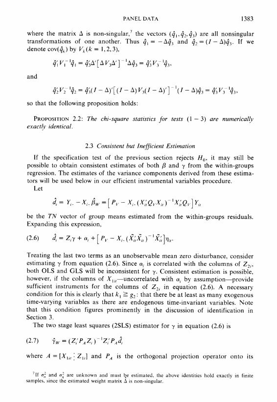
PANEL DATA 1383

where the matrix A is non-singular,7 the vectors (q q2 Aq3) are all nonsingular transformations of one another. Thus q, = -q3 and q2 = (I - )q3. If we denote cov(qk)by Vk(k= 1,2,3),

A iIAI= All[ 3/ 1 A

lv;'7I3, ql Il Iql q3Z\ \VZ q q3 q3 q3,

and

q2F V = -q3 V3(I- - q3= q3V3q3,

so that the following proposition holds:

PROPOSITION 2.2: The chi-square statistics for tests (1 - 3) are numerically exactly identical.

2.3 Consistent but Inefficient Estimation

If the specification test of the previous section rejects HO, it may still be possible to obtain consistent estimates of both ,B and y from the within-groups regression. The estimates of the variance components derived from these estima- tors will be used below in our efficient instrumental variables procedure.

Let

d, = Y. - Xi.,8w = [ PvXi. (Xi,QVXit), )Xj Qv] Yit

be the TN vector of group means estimated from the within-groups residuals. Expanding this expression,

A -

(2.6) d, = Z-y + a,. +[Pv- Xi. (XiX>,- ) Xi,]mIq.

Treating the last two terms as an unobservable mean zero disturbance, consider estimating -y from equation (2.6). Since a, is correlated with the columns of Z2 both OLS and GLS will be inconsistent for y. Consistent estimation is possible, however, if the columns of XI,, uncorrelated with a, by assumption provide sufficient instruments for the columns of Z21 in equation (2.6). A necessary condition for this is clearly that k- 9g2: that there be at least as many exogenous time-varying variables as there are endogenous time-invariant variables. Note that this condition figures prominently in the discussion of identification in Section 3.

The two stage least squares (2SLS) estimator for y in equation (2.6) is

(2.7) Yw (Zi PA Z ) Z PA di

where A = [X11j Zli] and PA is the orthogonal projection operator onto its

71f a2 and a2 are unknown and must be estimated, the above identities hold exactly in finite samples, since the estimated weight matrix A is non-singular.

1384 J. A. HAUSMAN AND W. E. TAYLOR

column space. The sampling error is given by

-Y Y (Z'PA ) 'ZPA[Pai + { P, Xi. (- ii,

and under the usual assumptions governing X and Z, the 2SLS estimator is consistent for -y, since for fixed T, plimN (l/(l/N)A'ao = 0 and plimNo(1/N)

= 0. The fact that the di are calculated from the within-groups residuals suggests that if P. is not fully efficient, then Yw may not be fully efficient either.

Having consistent estimates of / and under certain circumstances--y, we can construct consistent estimators for the variance components. First, a consis- tent estimate of a. can always be derived from the within-groups residuals. If Qx denotes ITN- X,(Xi',Xi,)-< X',, we can write the sum of squares of within-group residuals as

Yi'tQYit = 7i1Q-ij = Q 7It it (x ) Xjt

Thus

pliM 2 = pliM 1 YQY=pi 4 N-*oo N -oo N(T -1) NQoo N(T -1)

= plim N(_1) 21,Q71t

since rank ( Qv) = N(T - 1). Finally, whenever we have consistent estimators for both / and -y, a consistent

estimator for aa can be obtained. Let s2= ( 1/N)( Y. .-X,./3W- ZjYW)'(Y, -

X. i PW- Zi W); then

plims2= plim I (a. + -)'(a. + -)=a2+i2 Nv N-Xoc

so that s2 = -2 - (1/T)S2 is consistent for a2

3. INSTRUMENTAL VARIABLES ESTIMATORS

3.1 Identification

In this section, we discuss identification of some or all of the elements of (/3, y), using only the prior information in equations (2.2) and the time-invariant nature of the latent variable. Because the only component of the disturbance which is correlated with an explanatory variable is time-invariant, any vector orthogonal to a time-invariant vector can be used as an instrument. In particular, Qvai = 0 by construction, so that time-invariance provides at least TN - N

linearly independent instruments in equation (2.1): namely, TN - N basis vec- tors of the column space of Qv.

Unfortunately, as noted in the Introduction, Qv is also orthogonal to Zi, which violates the requirement that instruments be correlated with all of the explana-

PANEL DATA 1385

tory variables.8 The familiar results on identification in linear models are easily extended to cover this case: consider the canonical linear simultaneous equations model

(3.1) Y = X/ + e

where some of the k columns of X are endogenous and the matrix Z contains T observations on all variables for which plimT,(l / T)Z'e = 0. Project equation (3.1) onto the column space of Z:

(3.2) Pz Y = PzX,8 + Pze.

Now, if X is a k vector of known constants, we have the following lemma.

LEMMA: A necessary and sufficient condition for a particular (set of) linear function(s) X'/8 to be identifiable in equation (3.1) is that X'/8 be estimable in equation (3.2).

The proof follows readily from a result of F. Fisher [3, Theorem 2.7.2, p. 56]; details are available in Hausman-Taylor [7].

Using this result, it is easy to see that without any prior information in equations (2.2), all of the elements of /8 in equation (2.1) are identifiable. Simply project equation (2.1) onto the column space of all the exogenous variables- such a projection operator is Qv-and observe that all linear functions of /8 are estimable, since Xi,QvXi, is non-singular. No linear functions of y are estimable.9

If prior information is provided by equations (2.2) (i.e., k, > 0, g1 > 0), then the columns of X,1, and Z11 must be added to the list of instruments. Let A denote the matrix [ Qv* Xli* ZJ] and let PA be the orthogonal projection operator onto its column space. Then, corresponding to the familiar rank condition, we have the following proposition:

PROPOSITION 3.1: A necessary and sufficient condition that the entire vector of parameters (/3, y) be identified in equation (2.1) is that the matrix

Xit ...PA (Xit Zi)

Zi'

be non-singular.

Corresponding to the order condition, we have the following proposition:

PROPOSITION 3.2: A necessary condition for the identification of (/3, y) in equa- tion (2.1) is that k1- 9g2

8In this case, the order condition is grossly overfulfilled and the rank condition fails. 9This fact underscores the importance of the observation that the disturbance in equation (2.6) is

correlated with Zj, so that prior information from equations (2.2) is necessary to estimate y.

1386 J. A. HAUSMAN AND W. E. TAYLOR

PROOF: The rank condition follows from the Lemma. For the order condition, rank[PA (X1., Z1)] rank[PA4Xi] + rank[PAZi] = k + rank[PA4ZJ, so that a neces- sary condition for the matrix in Proposition 3.1 to be non-singular is that rank[PA Zi] - g. Since Z. is orthogonal to Qv, k -g2 is necessary for rank[PA Zi] to equal g, which completes the proof.

Identification in structural equations with panel data thus has a number of noteworthy features. First, given the assumption that a1 is correlated with the columns of X and Z, it is remarkable to find that the coefficients of the time-varying variables are identified while those of the time-invariant variables are not. Similarly, one variance component (ag) is identifiable while the other (as) is not. The parameters (y, a.) can be identified if the prior information (2.2) provides enough instruments-at least one for every endogenous column of Z1. Curiously, the k, exogenous columns of Xi, which are included in the structural equation (2.1) are the only candidates for these identifying instruments. This contrasts with the conventional simultaneous equations model in which excluded exogenous variables such as family background in the traditional measurement of the return to education are required to identify and estimate the parameters of a structural equation. Intuitively, this works because only the time-invariant component of the disturbance is correlated with (X2, Z2). Since XK1, = X111 + X11., X11, can be used as an instrument for X, and X11. can be an instrument for Z2i-

3.2 Estimation

When the parameters of equation (2.1) are identified by means of a specified set of variables which can be used as instruments, a consistent and asymptoti- cally efficient estimator for (/,, -y) can be constructed. Except for the fact that the disturbance covariance matrix Q is non-scalar, equations (2.1) and (2.2) represent an ordinary structural equation and a list of exogenous and endogenous variables from which the reduced form can be calculated. Thus if Q were known, 2SLS estimates of (/3, y) in

(3.3) Q2 1/2 yi = Q - /12X I,,8 + Q - t /2ZI. y + Q -2I i2e

taking X,, Z, as exogenous, would be asymptotically efficient in the sense of converging in distribution to the limited information maximum likelihood estima- tor.

More precisely, the information in equations (2.1) and (2.2) can be expressed as a system consisting of a single structural equation and two multivariate reduced form equations:

1/2 yi = Q - 12X1,, + Q - X/2Z.y + Q - I/2f

(3.4) X2it = Xli1l + Z1'7712 + QV7TI3 + Vli,

Z2= Xlit721 + Z11722 + QV723 + V2it1

PANEL DATA 1387

This system is a convenient form for discussing the efficiency of 2SLS estimators in equations (2.1) and (2.2). Equations (3.4) are triangular (because the bottom two equations are reduced forms) but not recursive (because v1 and v2 are correlated with ai). In addition, the reduced form equations are, of course, just-identified. Since the disturbance covariance matrix in equations (3.4) is unknown, OLS is inconsistent while 3SLS is fully efficient; see Lahiri-Schmidt [11]. Finally, since the reduced forms are just-identified, 3SLS estimates of ( 13, y) in the entire system are identical to 3SLS estimates of ( 13, -y) in the first equation alone (see Narayanan [161), and these are, of course, just the 2SLS estimates. Thus 2SLS estimates of (13, -y) in equation (3.3) are fully efficient in the sense that they coincide asymptotically with FIML estimators from the system (3.4).

Finally, 2SLS estimates of (1,, -y) in equation (3.3) are equivalent to OLS estimates of ( 1, -y) in

(3.5) pA 2yit = PAQ / Xit' + PA / 2ZiY + pA -

1ti

where PA is the orthogonal projection operator onto the column space of the instruments A = [Qv Z111 Least squares applied to this equation is com- putationally convenient: (i) the transformation Q- 1/2 can be done by (1 - 9)- differencing the data as in equation (2.5), (ii) the projection of the exogenous variables onto the column space of A yields the variables themselves, and (iii) the projection of the endogenous variables onto the column space of A can be calculated using only time averages, rather than the entire TN vectors of observations (see Appendix B).

For Q known, then, the calculation of asymptotically efficient estimators is straightforward; but the only case of practical interest is where Q is unknown and must be estimated. The question that immediately arises is how S2 should be estimated and whether an iterative procedure is necessary for efficient estimation of (13,y).

Consider the feasible analog of equation (3.5), where Q-1/2 is any consistent estimator for Q, e.g., from Section 2.3:

(3.6) 0A -1/2yt PA Q X + PA Q -i2ZiY + PA 2Eit.

PROPOSITION 3.3: For any consistent estimator Q of 0, OLS estimates of (1,-y) in equation (3.6) have the same limiting distribution as OLS estimates in equation (3.5), based upon a known U.

PROOF: For fixed T, it is straightforward to verify that VN 8[,1(Q)- 3(Q)]40; details are available in Hausman-Taylor [7].

We have thus shown that the 2SLS estimates of the parameters in equation (3.3)-using any consistent estimate of Q-are asymptotically efficient. These estimators are identical to OLS estimates of (13, -y) in equation (3.6); for future reference, we denote them by (,B* ,*).

1388 J. A. HAUSMAN AND W. E. TAYLOR

In Appendix A, we derive the following characteristics of (/*, *), depending upon the degree of over-identification. If the model is under-identified (k1 < g2), /3* = /Bw and A* does not exist. If the model is just-identified (k1 = g2), 3* = 1w and A* =

A as defined in equation (2.7). If the model is overidentified (k, > g2), (3'(, 9*) differ from and are more efficient than (j3BW, Y) Finally, following Mundlak [15], we explore the relationship between ,B* and the Gauss- Markov estimator, when the latter exists.

3.3 Testing the Identifying Restrictions

More efficient estimates of ,3 and consistent estimates of y require prior knowledge that certain columns of X and Z are uncorrelated with the latent ai. An important feature of our procedure is that when the parameters are over- identified, all of these prior restrictions can be tested. This is an extremely useful and unusual characteristic: unusual in that it provides a test for the identification of y, and useful since the maintained hypothesis need contain only the relatively innocuous structure of equation (2.1). It works, basically, because /3 is always identified and /3w provides a consistent benchmark against which all (or some) of the restrictions in equation (2.2) can be tested by comparing ,B* with /3w. The principles of such tests are outlined in Hausman [6], and extended in Hausman- Taylor [8].

The null hypothesis is of the form

Ho: plim N X a.= O and plim NZa.= O. N-*oo NN-*o N

Under Ho, both /3w and /* are consistent, while under the alternative, plim ,B* 7 plim /3w = /3; thus deviations of q = /3* - /3w from the zero vector cast doubt on the null hypothesis.

To form ax2 text based on q, premultiply equation (2.1) by QA2 1/2 - [,TN-

Zi(Zi'Z.) - IZ']Qi- 1/2 and consider the within-groups and efficient estimators for /3 in the transformed equation. Letting X* -QzQ- =2Xi,

(3.8) '2 = [(X*,PAX*) -X PA Qz - (X* QVX*) X* QvQz]Qi l/2y,

= DY*

where QVQZQ- I1/2 = Qv and y* = Q- l/2y has a scalar covariance matrix. The specification test statistic is given by

m= q q[cov(2)] q=q [cov(w) - cov(g*)] q

=q' [ JDD '] +

q

where the second equality follows from the asymptotic Rao-Blackwell argument in Hausman [6] and ( )+ denotes any generalized inverse. Following Hausman- Taylor [8], we have the next proposition.

PANEL DATA 1389

PROPOSITION 3.4: Under the null hypothesis, (J2m converges in distribution to a X2 random variable, where a 2 is any consistent estimate of a, and d = rank(D) = min[k, - g2,TN - k].

PROOF: From Propositions 4.1 and 4.2 of Hausman-Taylor [8], we obtain the limiting distribution of m and the fact that

rank(D) = min [rank(X*'PH ), rank(I - X*(X*'QvX*)- X*'Qv)j

where PH projects onto the orthocomplement of the column space of QV in the column space of A: i.e., onto the column space of [Xli. Zli]. Under the usual linear independence assumptions, the second term in brackets equals TN - k. For the first term, rank(X*'PH) = min[k, rank( QzPH)], and since PH = PZPH +

QZPH, rank( QZPH) = (k1 + g1) (g1 + g2) = (k, - g2). This specification test of the identifying restrictions in equation (2.2) has some

noteworthy features. The number of restrictions nominally being tested is k, + gl, in the sense that if any of the restrictions in equation (2.2) is false, q should differ from 0. Yet the degrees of freedom for the x2 test depend upon the number of overidentifying restrictions (k9-g2). Indeed, when the model is just-identified, ,B* = ]w (see Section 3.2), so that cq is identically zero and the degrees of freedom are zero. Finally, note that the alternative hypothesis does not require that any of the columns of X or Z be uncorrelated with ai. Hence all of the exogeneity information about X and Z is subject to test by this procedure.'0

4. ESTIMATING THE RETURNS TO SCHOOLING

Measuring the returns to schooling has received extensive attention lately, and much discussion has focused on the potential correlation between individual- specific latent ability and schooling. (See Griliches [4] for an excellent survey.) Since the sample we use does not contain an IQ measure, it would seem likely on a priori grounds that the schooling variable and ai are correlated. Yet as Griliches [4] points out, it is not clear in which direction the schooling coefficient will be biased. While a simple story of positive correlation between ability and schooling leads to an upward bias in the OLS estimate, a model in which the choice of the amount of schooling is made endogenous can lead to a negative correlation between the chosen amount of schooling and ability. In fact, both Griliches [4] and Griliches, Hall, and Hausman [5] find that treating schooling as endogenous and using family background variables as instruments leads to a rise in the estimated schooling coefficient of about 50 percent." Since our method does not

'0This test compares instrumental variables estimators under nested subsets of instruments: /3* uses [ Q, xI Z1] and /3w uses [ Q,]. If one wishes to test particular columns of XI or Z, for exogeneity, while maintaining a just-identifying set of instruments, a similar test can be con- structed by comparing (,B*,y*) with (,8w, Yw). If the model is overidentified under the main- tained hypothesis, compare (/3*,y*) using the different instruments. See Hausman-Taylor [8j for details.

"'Using a specification test of the type Wu [21] and Hausman [6] propose, we find a statistically significant difference between the IV and OLS estimates. Chamberlain [1] also finds a significant increase in the schooling coefficient, comparing OLS with estimates from his two factor model.

1390 J. A. HAUSMAN AND W. E. TAYLOR

require excluded exogenous instruments, it is of some interest to see if the estimated return to schooling remains higher than the OLS estimate.

Our sample consists of 750 randomly chosen prime age males, age 25-55, from the non-Survey of Economic Opportunity portion of the Panel Study on Income Dynamics (PSID) sample. We consider two years, 1968 and 1972, to minimize problems of serial correlation apart from the permanent individual component.'2 The sample contains 70 non-whites for which we use a 0-1 variable, a union variable also treated as 0-1, a bad health binary variable, and a previous year unemployment binary variable. The two continuous explanatory variables are schooling and either experience or age.'3 The PSID data do not include IQ. The National Longitudinal Survey (NLS) sample for young men would provide an IQ measure, but problems of sample selection would need to be treated (as in Griliches, Hall, and Hausman [5]) which would cause further econometric complications. Perhaps of more importance is the fact that for the NLS sample, IQ has an extremely small coefficient in a log wage specification (e.g., between .0006 and .002 in Griliches, Hall, and Hausman [5]); and if it is included in the specification, it has only a small effect on the schooling coefficient. Thus we use the PSID sample without an IQ measure, and our results should be interpreted with this exclusion in mind.

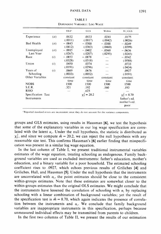
Table I gives the results of traditional estimators for our sample. The first two columns show the OLS and GLS estimates respectively, which assume no correlation between the explanatory variables and ai. The estimates are reason- ably similar, especially the schooling coefficient, which in both cases equals .067. The effects of experience and race stay the same, while the remaining three coefficients change somewhat, though they are not estimated very precisely. Note that the correlation coefficient across the four year period (p =.623) indicates that the latent individual effect is important. The finding that an additional year of schooling leads to a 6.7 percent higher wage is very similar to other OLS results from both PSID and other data sets.

In the third column of Table I, we present the within-groups estimate of the wage equation specification. All the time-invariant variables are eliminated by the data transformation, leaving only experience, bad health, and unemployed last year. As we have seen, the estimates of these coefficients are unbiased even if the variables are correlated with the latent individual effect. The point estimates change markedly from the first two columns: bad health by 26 percent, unem- ployment by 33 percent, and experience by 59 percent.'4 Comparing the within-

12Lillard and Willis [121 demonstrate within a random coefficients framework that a first order autoregressive process remains even after the permanent individual effect is accounted for. Our estimation technique can easily be extended to account for an autoregressive process, but for expository purposes we use a simpler case. Note that we are not investigating the dynamics of wages or earnings here.

13Experience was used as either experience with present employer or as (age - schooling - 5). Qualitatively, the results are similar, so we report results using the latter definition. As the results show, use of age yields very similar results for the schooling coefficient. Unlike Griliches [4], we are not attempting to separate the influence of age from that of experience.

'4Percentage changes are calculated as differences in natural logarithms.

PANEL DATA 1391

TABLE I

DEPENDENT VARIABLE: LOG WAGE

OLSa GLS Within IV/GLS

Experience (it) .0132 .0133 .0241 .0175 (.0011) (.0017) (.0042) (.0026)

Bad Health (it) -.0843 -.0300 -.0388 -.0249 (.0412) (.0363) (.0460) (.0399)

Unemployed (it) -.0015 -.0402 -.0560 -.0636 Last Year (.0267) (.0207) (.0295) (.0245)

Race (i) -.0853 -.0878 -.0542 (.0328) (.0518) (.0588)

Union (i) .0450 .0374 .0733 (.0191) (.0296) (.0434)

Years of (i) .0669 .0676 .0927 Schooling (.0033) (.0052) (.0191)

Other Variables constant constant constant constant time time time time

NOBS 1500 1500 1500 1500 S.E.R. .321 .192 .160 .193 RHO - .623 - Specification Test X2 = 20.2 2 = 8.70 Instruments father's ed.

mother's ed. poor

'Reported standard errors are inconsistent since they do not account for the variance components.

groups and GLS estimates, using results in Hausman [6], we test the hypothesis that some of the explanatory variables in our log wage specification are corre- lated with the latent ai. Under the null hypothesis, the statistic is distributed as X32 and since we compute m = 20.2, we can reject the null hypothesis with any reasonable size test. This confirms Hausman's [6] earlier finding that misspecifi- cation was present in a similar log wage equation.

In the last column of Table I, we present traditional instrumental variables estimates of the wage equation, treating schooling as endogenous. Family back- ground variables are used as excluded instruments: father's education, mother's education, and a binary variable for a poor household. The estimated schooling coefficient rises to .0927, which echoes previous results of Griliches [4] and Griliches, Hall, and Hausman [5]. Under the null hypothesis that the instruments are uncorrelated with ai, the point estimates should be close to the consistent within-groups estimates. Note that these estimates are somewhat closer to the within-groups estimates than the original OLS estimates. We might conclude that the instruments have lessened the correlation of schooling with ai by replacing schooling with a linear combination of background variables; yet the result of the specification test is mh = 8.70, which again indicates the presence of correla- tion between the instruments and ai. We conclude that family background variables are inappropriate instruments in this specification, perhaps because unmeasured individual effects may be transmitted from parents to children.

In the first two columns of Table II, we present the results of our estimation

1392 J. A. HAUSMAN AND W. E. TAYLOR

TABLE II

DEPENDENT VARIABLE: LOG WAGE

HT/IV IHT/GLS fIT/GLS HT/GLS HT/GLS

Experience .0217 .0217 - .0268 .024 h

(it) (.0027) (.0031) - (.0037) (.0045) Experience

Squared -.00012 (it) - - - (.00015)

Age .0147 (it) (.0028) - -

Bad Health -.0535 -.0278 -.0228 -.0243 -.0388 (it) (.0468) (.0307) (.0318) (.0318) (.0348)

Unemployment Last Year -.0556 -.0559 -.0634 -.0634 -.0560

(it) (.0311) (.0246) (.0265) (.0236) (.0279) Race -.0257 -.0278 -.0046 -.0014 -.0175

(i) (.0531) (.07518) (.0824) (.0662) (.0764) Union .1245 .1227 .1648 .1449 .2240

(i) (.0560) (.0473) (.0721) (.0598) (.2863) Years of

Schooling .1247 .1246 b 131 b .1315b .2169 (i) (.0380) (.0434) (.0490) (.0319) (.0979)

Other Variables constant constant constant constant constant time time time time time

NOBX 1500 1500 1500 1500 1500 S. E. R. .352 .190 .196 .189 .629 RHO - .661 .678 .674 .817 Specification

Test - 2= 2.24 _X = 0.0

'Reported standard errors are inconsistent since they do not account for the variance components.

bTreated as if correlated with a,.

method. We assume that X, contains experience, bad health, and unemployment last year, all initially assumed to be uncorrelated with ai. Z, is assumed to contain race and union status, while Z2 contains schooling, which is allowed to be correlated with al. The estimated schooling coefficient rises to .125, which is 62 percent above the original OLS estimate and 30 percent above the traditional instrumental variables estimate. The effect of race has now almost disappeared: its coefficient has fallen from -.085 in the OLS regression to -.028. The effects of experience and union status have risen substantially, while that of bad health has fallen.

Using the test from Section 3.3, we compare the within-groups and efficient estimates of the Xl coefficients. Observe that the unemployment coefficient is now very close to the within estimate, while bad health and experience have moved considerably closer to the within-groups estimates from either the OLS or instrumental variables estimates. The specification test statistic is m4 = 2.24 which is distributed as X2 under the null hypothesis of no correlation between the instruments and a.. While m is somewhat higher than its expected value of 2.0 under Ho0 we would not reject the hypothesis that the columns of X, and Z, are uncorrelated with the latent individual effect.

PANEL DATA 1393

We next examine how robust these estimates are to small changes in specifica- tion. Column 3 of Table II replaces experience with age. While experience is arguably correlated with ai through its schooling component, age can be taken as uncorrelated unless important cohort effects are present. The results are quite similar to our previous findings. The effect of schooling is .131, only slightly higher than the .125 found previously. Race again has little or no effect, while the coefficients of health and unemployment are similar to those in the specification with experience. In the next column of Table II, we include experience and experience squared as explanatory variables.'5 Again, the results are in general agreement with the original specification. The schooling coefficient increases from .125 to .132, and race still has little effect. We conclude that our main results are reinforced by these alternative specifications.

Our final specification relaxes some of the noncorrelation assumptions be- tween ai and the explanatory variables. We remove experience and unemploy- ment from the X, category, allowing them to be correlated with ai. Now X, contains only bad health. The model is just-identified, so that the efficient estimates of the coefficients of the Xi, variables are identical to the within-groups estimates. The specification test of Section 3.3 has zero degrees of freedom, and no specification test can be performed. The asymptotic standard errors have now risen to the point where coefficient estimates are quite imprecise, especially the schooling coefficient. Nevertheless, it is interesting to note that the point estimate of the schooling coefficient has risen to .217.

Thus all of our different estimation methods have led to a rise in the size of the schooling coefficient. Removing potentially correlated instruments has had a substantial effect: the point estimates change and their standard errors increase. All methods which control for correlation with the latent individual effects increase the schooling coefficient over those which do not; and this is certainly not the direction that many people concerned about ability bias would have expected.

5. SUMMARY

In this paper, we have developed a method for use with panel data which treats the problem of correlation between explanatory variables and latent individual effects. Making use of time-varying variables in two ways-to estimate their own coefficients and to serve as instruments for endogenous time-invariant variables-allows identification and efficient estimation of both /B and -y. The method is a two-fold improvement over the within-groups estimator: it is more efficient and it produces estimates of the coefficients of time-invariant variables. In the wage equation example, it performs better than traditional instrumental variables methods, which rely on excluded exogenous variables for instruments.

'5Neither of these alternative specifications pass the specification test if estimated by OLS and compared with the appropriate within-groups estimator. In both specifications, the latent individual effects are correlated with the explanatory variables.

1394 J. A. HAUSMAN AND W. E. TAYLOR

Perhaps most important, we derive a specification test of the appropriateness of the identifying exogeneity restrictions in equation (2.2). Since the within-groups estimates of /3 always exist and are consistent, they provide a benchmark against which further results-using the information in equations (2.2)-can be com- pared. If this specification test is satisfied, we can be confident in the consistency of our final results, since the maintained hypothesis embodied in the within- groups estimator is so weak.

Massachusetts Institute of Technology and

Bell Telephone Laboratories, Inc.

Manuscript received February, 1980; revision received October, 1980.

APPENDIX A

1. Special Cases

Depending upon (kl - g2). the degree of over-identification, the consistent and asymptotically efficient estimator (/3*, y*) exhibits some interesting peculiarities. Since we shall be interested in estimating /3 and y separately from equation (3.6), two generic formulae will prove convenient. Let Y = Xi /I + X2:2 + e.

LEMMA: The following two expressions for the OLS estimator of 81 are identical: (i) "parse out" X, bv premultiplving the model bv Q2 = I - X2(X2X2)- 2Xi, so that

/31 = (X |Q2X1Y) X'Q2Y:

(ii) remove the OLS estimates of X2,82 from Y and regress that on XI, so that

/, = (XX1) X[ 1 - X2(X 2QIX2Y)'XQl]

Now, suppose the parameters in equation (2.1) are under-identified. (a) k1 = g, = 0. Here, the set of instruments is only A = [Q.]. Since - 1/2=- _ -(I-_

PA Q- = so that 8*=/ w. (b) kI <g2. Here, the instruments are [Q. * Z . * XI. ] which we write as A = Qv * HI.

Consider equation (3.6). PAQ l 2Z = pH "2Z, since Q QI2Z - 0 When k < g QI z is not of full column rank since the dimension of the column space of H is g1 + k1 and Z, has g1 + g2

linearly independent columns. Thus there exists a g vector ( such that p4Q- '/2Zit = 0, so that yis not identifiable since y and (y + () are observationally equivalent in equation (3.6). To calculate /3*, "parse out" PAQ- 1/2Zi in equation (3.6) and run OLS. The column space of pA- /2 Zi equals the columnr space of H, so projecting pAQ- I72Xit onto the orthocomplement of P Q-- I/2Z yields QIXi,. Thus /3* = 8w in the generic underidentified case, and there is no consistent estimator for y.

Consider the just-identified case. (c) k, = g2. Here, again, the rank of P11Qi /2Zi equals the rank of H, so that /3* = 83w. The OLS

estimate of y in equation (3.6) is identical to the OLS estimate of y in

p Q - I/ 2 Y i j W = PA Q /2Zi y + PA 2,Ei, A 'F ~ = Z4

PANEL DATA 1395

by the previous Lemma, since /3w is the OLS estimate of /3 in equation (3.6). Thus y* can be written as

^ (Z Q- i/2p p- 1/2Z 1Z Q-I/2p [PA 1/2yit - pAS2 1/2 XitWI

( Z' Q-1P/2 p -i2z, )ZQ 1/2PAY -x . Xi. W]

(Zi'PA Zi) Zi'PA d = y

since Qi /2Z = OZ. For the just-identified case, then, our instrumental variables estimator coincides with the within-groups estimator of both /3 and y.

Suppose the parameters in equation (2.1) are over-identified. (d) k2 = 92 = 0. Here, A coincides with the explanatory variables in equation (3.6), so that the

2SLS and OLS estimators are identical. For 2- i/2 it is identical to the feasible GLS estimator in Section 2.1; for known 2 - 1/2 it is Gauss-Markov.

(e) k, > g2. The column rank of PAQ- 72Z is now g and the column space of PAQ- '/2Z differs from that of H. Thus /3* will differ from /w in the over-identified case. By the Lemma, y * is calculated from the regression of PAQ '72Y-PA?2 72X/s on P Q-I/2Z so that -y* will differ from -w, which we derived from the regression of PA Q - I 7X on PAQo '2Z.

Since (/3*,y*) are asymptotically efficient, (/3w, 'w) are inefficient in the over-identified case. Intuitively, this can be explained by regarding the within-groups estimators as 2SLS estimators which ignore the instruments Xli. and Zl. . It is a peculiar feature of this model that ignoring these instruments only matters when the parameters are over-identified.

2. Mundlak s Model

A final special case is the model discussed at length by Mundlak [15] in which no time-invariant observables are present and all explanatory variables are correlated with ai:

(A.l) Yi, = Xi,t + a? + ?it,.

The relationship between a and X is expressed by Mundlak through the "auxillary" regression ao = Xj-77 + wi where no prior information is assumed about g. Mundlak shows that (i) if ai is correlated with every column of Xi. (77 is unconstrained), the Gauss-Markov estimator for /3 is the within-groups estimator /3w, and (ii) if ai is uncorrelated with every column of Xi. (77 = 0), the G-M estimator for /3 is the GLS estimator /3GLS in equation (2.5), assuming 2 to be known.

Recognizing that case (i) is just-identified (kl = = 0) and case (ii) is overidentified (k2 = = 0) the discussion in (c) and (d) above shows that the 2SLS estimator /3* is identical to the G-M estimator in both cases. More to the point, if a is uncorrelated with some columns of X.. and correlated with others (77 obeys some linear restrictions), the model is overidentified (k, > g2 = 0) and case (e) above shows that /3* is asymptotically efficient relative to I8w. Thus it is only in the two extremes (i) and (ii) that /3[ or /36LS is appropriate.

We can use this characterization of the G-M estimator, however, to examine the relationship between /3* and the G-M estimator, should the latter exist. Suppose 2 is known, and we premultiply Mundlak's model (A.l) by 2- 1/2 and reparameterize for convenience:

(A.2) 2- 1/2 Yt = - 12Xit,SS - /? + ?2/2a? + 1- 2qit

= 2 -112M + ?*

where Mi, = X,S S = S - 1,, E.*= Oa + q,i- (I - 0)qi. = a?' + q?* and the non-singular transforma- tion S is chosen so that

S'(Xi'X1,)S= 'k

Since the Xi, are random variables in the analysis, the matrix S, being a function of the Xi,, will be random also; since some Xi, are endogenous S will also be endogenous.

1396 J. A. HAUSMAN AND W. E. TAYLOR

Let us specify prior information about the correlation between X,, and a in a somewhat more flexible manner than Mundlak's. Let h, denote the k vector of probability limits (for fixed T)

plim X' h = plim NS-'M,'a,ot S - hM VNX1!a N't1 N

where h,,1 denotes the corresponding vector of (asymptotic) correlations between ai and Mi,. We can express prior information on h, as r(r < k) homogeneous linear restrictions

Rh, = 0 = RS - 'Sh =_-R*hvm

which yield r homogeneous restrictions on hM. Note that (i) the exogeneity information in equations (2.2) can be expressed as Rh, = 0 where each row of R has a single I and the rest zeroes; (ii) the previous results on identification and estimation go through, taking the columns of Xi, R' as exogeneous where Ri(i = 1, . . ., r) is a row of R; (iii) homogeneous restrictions on h' correspond uniquely to homogeneous restrictions on-77 in Mundlak's specification; i.e., Rh, = 0 => Pl M N I:0

l /N) R(Xi'.XXi. ) (Xi'. Xi. )-'Xi'.ai Rzrk, = 0 where R = R (Xi'. Xi, .

In the model (A.2), then, certain linear combinations of the colums of Mi, are assumed uncorre- lated with a7* and all of the columns of Mi, are orthogonal.

PROPOSITION A.l: The 2SLS estimator , in equation (A.2) is Gauss-Markov for ,.

PROOF: Let F denote the k x k non-singular matrix

F= R' B']

where the columns of B'(k x k - r) are k - r basis vectors for the column space of IA - R'(RR')- 'R. Now, reparameterize equation (A.2) as

Q- 1/2y =y Q- 12Mi,FF- 't + E,

= Q- 1/2[ MitR' MitB]F F +

which we write as

(A.3) 2-2 /2yt = 52- 1/2L1i,tl + Q- 1/2L2it62 + (XT

where 6 = [SI * S,] = F- ',. Consider 2SLS estimates of 8 in equation (A.3), using as instruments A = [ Qv LJ,] since plimN (l/N)L',,a* = plim(l/N)RMi,2-lai = 0 by assumption. By con- struction, 2 LI and Q'72L2 are orthogonal, and PALI = LI, so the 2SLS estimator

61 = (Li,0- iL1j,) 'Llj,Q- '1,

coincides with the GLS estimator (for known 2). It is Gauss-Markov for 61 in this model since all columns of L, are uncorrelated with E* and L2 is orthogonal to LI. Similarly, the 2SLS estimator for 62 is

622= (L. i 2Q,Q- /212) lLQ i/2Q - i/2y

since P4L2 = QvL2. Since Q,Q-- /2= Qv. this simplifies to 6. =(LQtL,) -'L Qu,Y which is the within-groups estimator. Using Mundlak's result (i) above, 6* is G-M for 82 since every column of L, is correlated with a,, and L2 is orthogonal to LI. Hence '* = [61': 62']' is G-M for 6, and since F is a non-singular, non-stochastic matrix. = F6* is Gauss-Markov for FS = (. This completes the proof.

Two related questions immediately emerge. First, is /* = St* Gauss-Markov for ,B since S is non-singular? Secondly, what became of the intuition that 2SLS estimates were biased and thus not Gauss-Markov?

PANEL DATA 1397

PROPOSITION A.2: The 2SLS estimator /3* coincides with SS,* but /3* is biased for /3 and not Gauss- Markov.

PROOF: Calculate ,B* directly using 2SLS in the model

p Q-1/2y = p X Q -

I/X1,8/ +

PA&2 /72Ei,

where A = Ql Ll,] is the appropriate set of instruments here, as well as in equation (A.3). Then

= [Xi,Q -2/2 p 1/2X, ]- X - 1/2p 7 -1/2 y

=S[ SX52 -I/ 2PA 0 -

XS ISXQ - 2PA 0 1/2 y

= St*.

Thus ,B* is a non-singular transformation of the G-M estimator (*: i.e.,

/3=St* and 3- St

so that /*-/ = S(Z* - (). However, recall that S is a function of the matrix Xi,; it is endqgenous and in calculating moments of 3* - /, we cannot condition on it. Hence, in general, E(/3* - /3) = ES($* - + SE($-* = 0, and cov[/8* - /] = cov[S((*- )] -

S[cov(Q - ()]S' where cov($* - () attains the Cramer-Rao bound.

A final anomalous property of /3* follows from these propositions. Suppose the original design matrix Xi, were orthogonal, so that Xi'Xi, = 'k. Then the 2SLS estimator /* using [Qv Xt,R'] as instruments would be both unbiased and Gauss-Markov. One rarely finds a G-M estimator in a simultaneous equations problem; one does in this model because 2SLS estimates when all the explanatory variables are correlated with ai are identical to the within-groups estimators, and these are unbiased in finite samples. This is because the set of instruments in this model is just the columns of Qv, which are orthogonal to ai in the sample, not just in expectation or as a probability limit.

APPENDIX B

Computational Details

We now consider the estimation method proposed in Section 3.2 from the standpoint of computational convenience. Equation (3.6) and Proposition 3.3 state the basic theoretical results. Given initial consistent instrumental variables estimates of ( /, y), we can estimate Q and transform the variables by 0-differencing the data. The model now is of the form of equation (3.6) and OLS estimates will be asymptotically efficient.

The main difficulty that arises is computational: how to do instrumental variables when the data matrix (of order T x N) may exceed the computational capacity of much econometric software. If this occurs, using equation (3.4), calculate predicted values of X2 and Z2 from their reduced forms. The predicted Z2i's are formed from a sample size N regression of Z2i on the columns of X1i. and Z1i. For the X2,'s, rather than doing a sample size T x N regression, an equivalent procedure is to form X2i, = Xi- X2. + X2i. . The last term, X2i. , is calculated from the sample size N regression of X2i. on X1i. and Z1i. Then the calculated X2;, and Z2i are used with the Xl, and the Zl in an OLS regression to obtain consistent estimates of both /3 and y.16 A similar technique works with the transformed variables in equtation (3.6) which yields asymptotically efficient estimates of /3 and y. The reason that calculating X2i, in this manner is equivalent to the more cumbersome approach of a T x N sample regression of X2i, on instruments as indicated in equation (3.4) is that Qv is orthogonal

160ne note of caution, however. The estimates of the variance from the second stage are inconsistent, for the same reason that doing 2SLS in two steps yields inconsistent variance estimates in the second stage. One must use the estimated coefficients and equation (2.1) without the estimated variables on the right hand side.

1398 J. A. HAUSMAN AND W. E. TAYLOR

to any time-invariant variable. Thus parsing out Qv in the second and third equations of (3.4) is equivalent to premultiplying them by PV. and X2i. and Z2i can be calculated from the sample size N regressions on X1i. and Z,.. To get X2i,, we must add QV713 to X2., so that X21, is given by X2i, + X2,. -

If computational capacity is not a difficulty, a standard instrumental variables package can be used, with Xli,, X i., X2ji, and Zl as instruments. The variables which are time invariant have T identical entries for each individual i. So long as Proposition 3.1 is satisfied, the parameters are identified and the number of columns of X1i. is at least as great as the number of columns of Z2i (i.e., k g92). Note again how the columns of Xli, serve two roles: both in estimation of their own coefficients and as instruments for the columns of Z2i-

REFERENCES

[1] CHAMBERLAIN, G.: "Omitted Variable Bias in Panel Data: Estimating the Returns to Schooling," Annales de l'INSEE, 30/31,(1978), 49-82.

[2] CHAMBERLAIN, G., AND Z. GRILICHES: "Unobservables with a Variance Components Structure: Ability, Schooling, and the Economic Success of Brothers," International Economic Review, 16(1975), 422-449.

[3] FISHER, F.: The Identification Problem in Econometrics. New York: McGraw-Hill, 1966. [4] GRILICHES, Z.: "Estimating the Returns to Schooling: Some Econometric Problems,"

Econometrica, 45(1977), 1-22. [5] GRIIICHES, Z., B. HALL, AND J. HAUSMAN: "Missing Data and Self-Selection in Large Panels,"

Annales de l'INSEE, 30/31(1978), 137-176. [6] HAUSMAN, J.: "Specification Tests in Econometrics," Econometrica, 46(1978), 1251-1272. [7] HAUSMAN, J., AND W. TAYLOR: "Panel Data and Unobservable Individual Effects," M.I.T.

Discussion Paper, January, 1980. [8] "Comparing Specification Tests and Classical Tests," M.I.T. Discussion Paper, Septem-

ber, 1980. [9] HOCH, I.: "Estimation of Production Function Parameters and Testing for Efficiency,"

Econometrica, 23(1955), 325. [10] JORESKOG, K.: "A General Method for Estimating a Linear Structural Equation System," in

Structural Equation Models in the Social Sciences, ed. by A. S. Goldberger and 0. D. Duncan. New York: Seminar Press, 1973.

[11] LAHIRI, K., AND P. SCHMIDT: "On the Estimation of Triangular Structural Systems," Econometrica, 46(1978), 1217-1222.

[12] LILLARD, L., AND R. WILLIS: "Dynamic Aspects of Earning Mobility," Econometrica, 46(1978), 985-1012.

[13] MADDALA, G. S.,: "The Use of Variance Components Models in Pooling Cross Section and Time Series Data," Econometrica, 39(1971), 341-358.

[14] MUNDLAK, Y.: "Empirical Production Function Free of Management Bias," Journal of Farm Economics, 43(1961), 44-56.

[15] : "On the Pooling of Time Series and Cross Section Data," Econometrica, 46(1978), 69-86.

[16] NARAYANAN, R.: "Computation of Zellner-Theil's Three Stage Least Squares Estimates," Econometrica, 37(1969), 298-306.

[17] NERLOVE, M.: "A Note on Error Components Models," Econometrica, 39(1971), 359-382. [181 PUDNEY, S.: "The Estimation and Testing of Some Error Components Models," London School

of Economics Discussion Paper, 1979. [191 SCHEFFE, H.: The Analysis of Variance. New York: John Wiley & Sons, 1959. [201 TAYLOR, W.: "Small Sample Considerations in Estimation from Panel Data," Journal of

Econometrics, 13(1980), 203-223. [211 Wu, D.: "Alternative Tests of Independence Between Stochastic Regressors and Disturbances,"

Econometrica, 41(1973), 733-750.