PALAEOCLIMATE ANALYSIS

OF SOUTHWESTERN YUKON TERRITORY

USING SUBFOSSIL CHIRONOMID REMAINS

FROM ANTIFREEZE POND

Erin Margaret Barley

B.Sc., University of Guelph, 1998

THESIS SUBMITTED IN PARTIAL FULFILLMENT OF THE REQUIREMENTS FOR THE DEGREE OF

MASTER OF SCIENCE

in the Department of Biological Sciences

OErin Margaret Barley 2004

SIMON FRASER UNIVERSITY

July 2004

All rights reserved. This work may not be reproduced in whole or in part, by photocopy or other means,

without permission of the author.

APPROVAL,

Name: Erin Margaret Barley

Degree: Master of Science

Title of Thesis:

PALAEOCLIMATE ANALYSIS OF SOUTHWESTERN YUKON TERRITORY USING SUBFOSSIL CHIRONOMID REMAINS FROM ANTIFREEZE POND

Examining Committee:

Chair: Dr. C. Lowenberger, Professor

Dr. R. Mathewes, Professor, Senior Supervisor Department of Biological Sciences, SFU

Dr. I. Walker, Adjunct Professor Department of Biological Sciences, SFU

Dr. J. Clague, Professor Department of Earth Sciences, SFU

Dr. I. Hutchinson, Professor Department of Geography, SFU Public Examiner

Date Approved:

. . 11

Partial Copyright Licence

The author, whose copyright is declared on the title page of this work, has

granted to Simon Fraser University the right to lend this thesis, project or

extended essay to users of the Simon Fraser University Library, and to

make partial or single copies only for such users or in response to a

request from the library of any other university, or other educational

institution, on its own behalf or for one of its users.

The author has further agreed that permission for multiple copying of this

work for scholarly purposes may be granted by either the author or the

Dean of Graduate Studies.

It is understood that copying or publication of this work for financial gain

shall not be allowed without the author's written permission.

The original Partial Copyright Licence attesting to these terms, and signed /

by this author, may be found in the original bound copy of this work,

retained in the Simon Fraser University Archive.

Bennett Library Simon Fraser University

Burnaby, BC, Canada

ABSTRACT

Freshwater midges, consisting of Chironomidae, Chaoboridae and Ceratopogonidae,

were assessed as a biological proxy for palaeoclimate in Beringia. The Beringia training

set consists of midge assemblages and data for 25 environmental variables collected from

12 1 lakes in Alaska, British Columbia, Yukon and the Northwest Territories. Canonical

correspondence analyses revealed that lake depth, mean July air temperature and seven

other variables contributed significantly to explaining the midge distributions. Weighted

averaging partial least squares (WA-PLS) was used to develop midge inference models

for transformed depth (In (x+l); r2bo,,t=0.43 1, and RMSEP=0.574) and mean July air

temperature (r2b,ot=0.507, RMSEP=l .34SoC).

Antifreeze Pond in the southwest Yukon provides one of the oldest lacustrine records in

eastern Beringia, though a precise chronology for the lower core remains elusive. Mean

~ u l y air temperature and lake depth were inferred for the record using the WA-PLS

models as well as the Modem Analogue Technique (MAT). Midge analysis revealed a

sequence of five distinctive biostratigraphic zones that show general agreement with an

existing pollen record (Rampton, 197 1). Midge inferences point to a transition fi-om cold

and arid to warm and likely wetter conditions in the lower core. Midge remains were

extremely rare through the organic poor middle zone; extrapolation from adjacent zones

points to temperatures at least 2-3•‹C below modern. Temperature warmed to modem by

12,500 "C yr BP, then cooled again from 10,800 to 8,500 14c yr BP. By 8,000 "C yr

BP, inferred temperatures recovered to modem, and varied little through the rest of the

Holocene.

DEDICATION

To my grandfather Maurice V. Smith whose constant engagement with the natural world

is truly infectious.

ACKNOWLEDGEMENTS

Many people contributed directly and indirectly to this research. Thanks to Les

Cwynar for putting together such an interesting and enticing project, and to

Bronwen Whitney, Josh Kurek and the project collaborators for contributions of

data, ideas and enthusiasm.

In the lab at Okanagan University College, Christina Bleskie, Lydia Stepanovic,

Shelley MacIsaac, Sandra Rosenberg and the research assistants contributed to the

more laborious aspects of the project, and fueled the lab with an endless source of

energy and creativity. At Simon Fraser University, Grant Zazula was a tremendous

resource for all things Beringian, Marian McCoy offered her ears as a soundboard

for my ideas, and Terri Lacourse helped with the hows and whys of the palaeo

world.

Data was provided by Rene Gregory-Eaves and Andre Levesque. Steve Juggins'

program c2 and his prompt assistance were invaluable in the analysis and graphing

of data. Funding was generously provided by a CRO from NSERC (to Les Cwynar

as PI), and an NSTP grant to the author for fieldwork in the Yukon.

The examining committee of Rolf Mathewes, Ian Walker, John Clague and Ian

Hutchinson provided interesting questions and discussion during the exam, and

useful comments on the thesis. An additional thanks to Rolf for keeping me

focussed, and especially to Ian Walker for inspiration, knowledge and patience.

TABLE OF CONTENTS

. . Approval Page.. . . . . . . . . . . . . . . . . . . . . . . . . . . . .. . . . . ..... . . . . . . . . . . . . . . . . ..... . . . . . . . . . . . . . . . . . . . ...... 11 . . . Abstract ............................................................................................. 111

. . Ded~cation ...........................................,.............,.....................+......... iv ~cknowledgements . . . . . . . . . . . . . . . . . . . . . . . . . . . . . . . . . . . . . . . . . . . . . . . . . . . . . . . . . . . . . . . . . . . . . . . . . . . . . . . v Table of Contents.. . . . . . . . . . . . . . . . . . . . . . . . . . . . . . . . . . . . . . . . . . . . . . . . . . . . . . . . . . . . . . . . . . . . . . . . . . . . ... vi . . . List of Tables.. . . . . . . . . . . . . . . . . . . . . . . . . . . . . . . . . . . . . . . . . . . . . . . . . . . . . . . . . . . . . . . . . . . . . . . . . . . . . . . . . . . VIII

List of Figures.. . . . . . . . . . . . . . . . . . . . . . . . . . . . . . . . . . . . . . . . . . . . . . . . . . . . . . . . . . . . . . . . . . . . . . , . . . . . . . . .... Chapters

1 Introduction. . . . . . . . . . . . . . . . . . . . . . . . . . . . . . . . . . . . . . . . . . . . . . . . . . . . . . . . . . . . . . . . . . . . . . . . .

2 Literature Review 2.1 Palaeoecology of Eastern Beringia

2.1.1 Geography.. . . . . . . . . . . . . . . . . . . . . . . . . . . . . . . . . . . . . . . . . . . . . . .. . . . . . ... 2.1.2 The Palaeoenvironment from 26,000 to 10,000 ' 4 ~ yr BP. 2.1.3 The Palaeoclimate from 26,000 to 10,000 14c yr BP.. . . . . .

2.2 Chironomids as Indicators of Past Environments 2.2.1 Chironomids in Lake Sediments. . . . . . . . . . . . . . . . . . . . . . .. . . . . . . .. 2.2.2 Sensitivity to Environmental Variables. . . . . . . . . . . . . . . . . . . . . . . 2.2.3 Transfer Functions. . . . . . . . . . . . . . . . . . . . . . . . . . . . . . . . . . . . . . . . . . . . . . .

3 Development of Midge Inference Models for Beringia Introduction. . . . . . . . . . . . . . . . . . . . . . . . . . . . . . . . . . . . . . . . . . . . . . . . . . . . . . . . . . . . . . . . . Methods 3.2.1 Study Area.. . .. . . . . . . . . . . . . . . . .. . . . . . . . . . . . . . . . . . . . . . . . . . . . . . . . . . .. 3.2.2 Midge Analysis. . . . . . . . . . . . . . . . . . . . . . . . . . . . . . . . . . . . . . . . . . . . . . . . . . . 3.2.3 Environmental Variables. . . . . . . . . . . . . . . . . . . . . . . . . . . . . . . . . , . . , . . . Data Analysis 3.3.1 Datascreening .................................................... 3.3.2 Ordinations. . . . . . . . . . . . . . . . . . . . . . . . . . . . . . . . . . . . . . . . . . . . . . . . . . . . . . . . 3.3.3 Model Development . . . . . . . . . . . . . . . . . . . . . . . , . . . . . . . . . . . . . . . . . . .. . Results 3.4.1 Faunistic Description.. . . . . . . . . . . . . . . . . . . . . . . . . . . . . . . . . . . . . . . . . . . 3.4.2 Ordinations. . . . . . . . . . . . . . . . . . . . . . . . . . . . . . . . . . . . . . . . . . . . . . . . . . . . . . .. 3.4.3 Model Development. . . . . . . . . . . . . . . . . . . . . . . . . . . . . . . . . . . . . . . . . . . . . . Discussion 3.5.1 Fauna.. . . . . . . . . . . . . . . . . . . . . . . . . . . . . . . . . . . . , . . . . . . . . . . . . . . . .... . .. . . . 3.5.2 Models and Training Set.. . . . . . . . . . . . . . , . . . . . . . . . . . ..... . . . . . . . . .

4 A Palaeoclimatic Reconstruction for Antifreeze Pond, Yukon Territory 4.1 Introduction . . . . . . . . . . . . . . . . . . . . . . . . . . . . . . . . . . . . . . . . . . . . . . . . . . . . . . .... . . . . .. 4.2 Study Area.. . . . . . . . . . . . . . . . . . . . , . . . . . . . . . . . . . . . . . . . . . . . . . . . . . . . . . . .... . . . . .

4.3 Methods 4.3.1 Field and Laboratory Methods .................................. 52 4.3.2 Chronology ....................................................... 52 4.3.3 Data Analysis ..................................................... 61

4.4 Results 4.4.1 Midge Stratigraphy ............................................... 62 4.4.2 Temperature and Depth Reconstructions ..................... 66

4.5 Discussion and Regional Synthesis ..................................... 76

5 Conclusion .......................................................................... 84

References ........................................................................................ 87 Appendix .......................................................................................... 99

vii

LIST OF TABLES

Table 2.1

Table 2.2

Table 3.1

Table 3.2

Table 3.3

Table 3.4

Table 3.5

Table 3.6

Table 4.1

Table 4.2

Table 4.3

Table 4.4

A selection of Beringian pollen studies covering the herb zone 14 ...................................... (approx. 30,000 to 14,000 C yr BP). 7

A selection of Beringian pollen studies covering the birch zone 14 (approx. 14,000 to 10,000 C yr BP). ..................................... 9

The Beringia training set: environmental, limnological and chemical data for 12 1 lakes.. ............................................................ 22

Variance explained before and after forward selection in CCA. Results are presented for: run 1) CCA with covariables AK, KW and U, and all variables selected in the order presented; run 2) CCA with covariables AK, KW and U, TPU selected first, and all other variables selected in the order presented; run 3) CCA without covariables, and all variables selected in the order presented; and run 4) CCA without covariables, JTEMP selected first, and all other variables selected in the order presented.. ................................. 35

Eigenvalues, taxon-environmental correlations, cumulative % ......... variance and significance of the four axes for the final CCA.. 37

Canonical coefficients, their t-values and interset correlations for the final CCA. ...................................................................... 38

A comparison of WA and WA-PLS models for reconstructing a) depth, and b) mean July air temperature.. .................................. 42

Values for all non-rare taxa for: taxon occurrence (i.e., percentage of 12 1 lakes in which taxon was present), and for each of depth and mean July air temperature: taxon range, WA optimum (bootstrapped), WA tolerance (bootstrapped) and WA-PLS Beta coefficient (bootstrapped). ................................................... 43

AMS radiocarbon dates for Antifreeze Pond.. ............................ 53

A comparison of the theoretical contamination required to produce the three different radiocarbon dates at 450 cm ............................. 58

Bulk sediment radiocarbon dates from Rampton (197 1). ................ 60

Raw midge data (number of head capsules recovered) for intervals 260 to 360 cm of Antifreeze Pond.. ......................................... 65

... Vll l

LIST OF FIGURES

Figure 3.1

Figure 3.2

Figure 3.3

Figure 3.4

Figure 3.5

Figure 3.6

Figure 4.1

Figure 4.2

Location of 12 1 lakes of the Beringia training set. Outliers are .................................................... identified by open circles

A chironomid diagram for the Beringia training set, with taxa ranked by latitude (N to S) as determined by a constrained CCA. All taxon abundances are presented as a % of the total identifiable chironomids. Taxa that were rare or never exceeded 5% have been omitted. Vegetation type is indicated at right with some abbreviations: T-ARC, arctic tundra; T-ALP, alpine tundra; L- WOOD, lichen woodland .......................................................

A chironomid diagram for the Beringia training set, with select taxa ranked by mean July air temperature (cold to warm) as determined by a constrained CCA. All taxon abundances are presented as a % of the total identifiable chironomids.. ..........................................

A chironomid diagram for the Beringia training set, with select taxa ranked by mean depth (shallow to deep) as determined by a constrained CCA. All taxon abundances are presented as a % of the total identifiable chironomids.. ................................................

Canonical correspondence analysis ordination showing the dispersion of sites by vegetation type, relative to nine significant environmental variables ...................................................

Canonical correspondence analysis ordination showing the dispersion of taxa relative to nine significant environmental variables. Taxon codes correspond with full taxon names listed in Table 3.6 .....................................................................

.... Map locating Antifreeze Pond in southwestern Yukon Territory

A-C) Depth-age profiles for Antifreeze Pond, showing all AMS radiocarbon dates with errors (small error bars not visible). In the upper core, linear interpolation (solid lines) between accepted dates was used to create a depth-age model. For the lower core, three possible chronologies (broken lines) are illustrated: A) chronology 1, B) chronology 2 and C) chronology 3. Source of dated material:

terrestrial or emergent macrofossils (accepted), 0 terrestrial or emergent macrofossils (rejected in the upper core, status uncertain in the lower core), chironomid head capsules (status uncertain), A aquatic macrofossils (status uncertain). D) A loss on ignition (LOI) curve for Antifreeze Pond. The LO1 curve, with midge based zonation, is included as it reflects changes in sediment composition ...

Figure 4.3 A chironomid stratigraphy for Antifreeze Pond. Select taxa are sh~wn, and all taxon abundances are presented as a % of the total identifiable chironomids. Data is presented for intervals with greater than 15 chironomid head capsules; intervals with low counts (1 5-35

.......................... chironomid head capsules) are indicated by a + 63

Figure 4.4 An analogue comparison of intervals from Antifreeze Pond with sites from the Beringia training set. Intervals with squared chord distances below the 75% confidence interval have good analogues, those between 75% and 95% have weak analogues, and those greater than 95% have no analogues. Intervals with low counts (15-35 chironomid head capsules) are indicated by a + .......................... 67

Figure 4.5 Mean July air temperatures as inferred by WA-PLS and MAT. Lowess smooths (thick lines) are superimposed on the temperature curves (thin lines). Error bars represent sample specific bootstrapped squared errors of prediction. The modern mean July air temperature of 13.2"C is plotted for reference. Intervals with low

......... counts (1 5-35 chironomid head capsules) are indicated by a + 69

Figure 4.6 Depths as inferred by WA-PLS and MAT. The potential overflow level is plotted for reference. Lowess smooths (thick lines) are superimposed on the depth curves (thin lines). Error bars represent sample specific bootstrapped squared errors of prediction. Intervals with low counts (1 5-35 chironomid head capsules) are indicated by a

Figure 4.7 A correlation of the midge record with Rampton's (1 97 1) pollen record ............................................................................. 7 1

Figure 4.8 Mean July air temperatures for the late glacial and Holocene as inferred by WA-PLS and MAT, and plotted against age. Lowess smooths (thick lines) are superimposed on the temperature curves (thin lines). Error bars represent sample specific bootstrapped squared errors of prediction. The modern mean July air temperature of l3.2"C is plotted for reference. Intervals with low counts (1 5-35 chironomid head capsules) are indicated by a + .......................... 75

1 Introduction

Climate has always impacted humans, influencing both where we live at regional and

global scales, and how we feed and shelter ourselves. Cultures have thrived during

periods of climatic stability only to weaken or disappear with changes in temperature,

precipitation, or frequency of climate driven disasters (Brenner et al., 2002; Nufiez et al.,

2002). For all of human existence, climate has been a dynamic system. However, it is

only in the past century that we have really begun to understand the components and

processes which influence climate, and to recognize the roles they play in driving climate

change (Bradley, 1999).

With a growing understanding of climate comes a new awareness of the potential effects

of global climate change. Changes in precipitation and temperature threaten current

agricultural regions, clean water sources, and communities dependent on a stable sea-

level (Government of Canada, 2003). Our greatest asset in dealing with these threats is

an ability to foresee what changes will occur, and how they will unfold. This requires

sound knowledge of past climates, in order to understand the long term cycles and

patterns ofclimate change. It is only by studying past changes, and the effects these had

on past peoples and environments, that we begin to understand our current predicament,

and to properly prepare for the future.

During the Last Glacial Maximum1 (LGM, 26,000 - 14,000 I4c yr BP), much of the

Northern Hemisphere was covered by glaciers that scoured away sediments, erasing the

palaeoecological records they contained (Bradley, 1999). Undisturbed by these glaciers

was Beringia, a region extending from the Yukon, through Alaska, across the exposed

Bering Land Bridge and into Siberia. With sediments extending back through the late

Pleistocene, Beringia is an extensive repository for palaeoclimatic and palaeoecological

data (Elias, 200 1 a). Beringia is located at sub-arctic and arctic latitudes, making it

particularly sensitive to climate change. Extensive permafrost and short growing seasons

1 Terminology follows Elias (200 la).

characterize the modem landscape, and even small changes in climate can have

pronounced effects on the environment and the life it contains.

To date, palaeoclimates in Beringia have been inferred primarily from pollen records.

The full glacial was cold and dry, with increases in temperature and moisture through the

late glacial before reaching near modem conditions at the start of the Holocene (Elias et

al., 1996; Lozhkin et al., 1993). However, the broad picture of climate painted by pollen

records contributes little to the quantitative data needed to answer questions such as: how

cold and dry was the full glacial? How rapidly did climate ameliorate through the late

glacial? Was the amelioration punctuated by any reversals? Beetle data obtained by

Elias (2000,20Olb), provide the first quantitative estimates of temperatures during the

full glacial, suggesting summer temperatures 2-4•‹C colder, and winter temperatures 8•‹C

colder than at present.

Chironomids, as well as Ceratopogonidae and Chaoboridae, constitute the freshwater

midges, another insect group whose usefulness as a palaeoclimatic indicator has been

demonstrated (Porinchu and MacDonald, 2003; Walker et al., 1997). Chironomid-

temperature transfer functions have been developed, that allow for the reconstruction of

mean July temperatures with errors of less than 2•‹C (Porinchu and MacDonald, 2003).

When applied to lake sediment records with good chronology, these provide excellent

high resolution temperature reconstructions. Similarly, where significant changes in lake

depth have occurred, chironomid-depth transfer functions can illustrate these changes

(Korhola et al., 2000). As an independent indicator of palaeoclimates, chironomids have

the potential to contribute new and much needed high resolution data, and to further our

understanding of the nature of past climate changes.

The objectives of the research presented here are two-fold: 1) to create midge-

temperature and midge-depth transfer functions for western Canada and Alaska, and 2) to

reconstruct palaeoclimates of Eastern Beringia from midge analysis of Antifreeze Pond in

southwest Yukon.

2 Literature Review

2.1 Palaeoeccdogy of Eastern Beringia

2.1.1 Geography

In 1937 Hultkn hypothesized a land bridge connecting Alaska to Siberia and called this

land Beringia, after the Bering Strait (in Hopkins, 1996). Since then, the concept of

Beringia has expanded to include contiguous regions to the east and west that remained

unglaciated during the last glacial period. The western limit of Beringia is recognized as

the Lena River in Siberia. This is a practical boundary and somewhat arbitrary as the ice-

free landscape continued and expanded westward into Eurasia, with glaciers restricted to

the Chukotka Mountains (Alfimov and Berman, 2001). Eastern Beringia is more clearly

demarcated by glacial boundaries along the Alaska and Coastal Ranges in the south, and

in the east by the Laurentide Ice Sheet reaching to the eastern foot of the Richardson

Mountains (Hughes, 1972).

Eastern Beringia's mountains run east-west with the Brooks and Cordilleran Range

located in the north and the Alaska and Coastal Range in the south. Most other features

such as the major river systems and vegetation zones, run parallel to the mountains. To

the far north is tundra; between the mountain ranges, uplands and lowlands alternate and

boreal forest dominates with regions of muskeg. Coastal forest is found along the

southern (formerly glaciated) foot of the mountains (Anderson and Lozhkin, 2001 ;

Ritchie, 1984).

The modem vegetation of Eastern Beringia consists mainly of boreal forest and tundra

(Anderson and Lozhkin, 2001 ; Muhs et al., 2001 ; and Ritchie, 1984). The forests are

dominated by Picea glauca (Moench) Voss and Picea mariana Mill., and filled out by

other tree species including Larix laricina (Du Roi) K. Koch, Betula papyrifera Marsh.,

Populus balsamifera L., and Populus tremuloides Michx. Tundra is found in the north,

and at higher elevations. Poaceae and Cyperaceae dominate with shrubs of Salix and

Betula. Other vegetational types are scattered across the landscape including fell-field at

high elevations and steppe slopes in areas too dry to support trees (Laxton et al., 1996).

Climate in Alaska and the Yukon varies with distance from the oceans and local

topography. In thc north, air temperatures are influenced by the perennially frozen Arctic

Ocean and are cold year round. In most of the Yukon and central Alaska, a continental

climate creates warm summers and cold winters, with a temperature range of 40•‹c

between the warmest and coldest months (Phillips, 1990). High air pressure and long

days provide abundant clear sunny skies and an accumulation of summer heat. In winter,

temperature inversions can lead to cold air in the valleys, with less extreme temperatures

at higher elevations. Precipitation is moderate and peaks in late summer. Topography

also has a strong influence on precipitation, with the wettest regions located on the south

and west slopes of mountains. In the south, Alaska is under a maritime influence, and has

a more moderate climate. Precipitation increases with proximity to the Pacific; inland,

moderate levels of precipitation peak in late summer. Permafrost ranges from continuous

through most of the north, to sporadic in southern Yukon (Natural Resources Canada,

2003).

2.1.2 The Palaeoenvironment from 26,000 to 10,000 I4c yr BP

For over a century, miners and researchers in Beringia have been digging up fossils

belonging to an interesting and now extinct assemblage of large mammals including

mammoths, camels, bison, mastodons, horses, saber-toothed cats, giant beavers, and

saiga antelope. In 1968, Guthrie, a mammalogist, published the first of a series of papers

that sparked a vigorous debate over the character of the full glacial landscape in Beringia.

From fossil records, including tooth morphology and stomach content of some frozen

specimens, and observations of close relatives of the extinct species, he determined that

the large fauna was predominantly composed of grazers, and secondarily browsers

(republished in Guthrie, 1996). Guthrie reasoned that a more productive than present

vegetation must have been necessary to support the diversity and dietary requirements of

this megafauna. Guthrie put forth the hypothesis that the fauna was supported by a

'mammoth steppe', an extensive grassland contiguous with that of Eurasia. He proposed

(Guthrie 1982, 1985) that it had the following properties:

fertile and productive soils capable of providing sufficient quality and quantity of

forage

herbaceous vegetation with lots of grasses that were high in nutrients, and low in

antiherbivory components

a deeper thaw and longer growing season than at present

shallow snow cover (from low snowfall and/or windy conditions) to permit winter

grazing and browsing by fauna

a firm dry substrate to support the foot morphology of the fauna

a diversity of habitats to support varying dietary requirements

In a series of publications, Ritchie and Cwynar (Cwynar, 1982; Cwynar and Ritchie,

1980; Ritchie, 1984; Ritchie and Cwynar, 1982) challenged Guthrie's proposal of a

mammoth steppe, based on pollen analyses of cores from two northern Yukon lakes. For

the herb zone (33,000 to 14,000 I4c yr BP), they note low pollen influx values suggesting

sparse vegetation. They found pollen taxa of arctic and alpine vegetation, and interpreted

the Artemisia and grass dominated assemblage to be analogous to the modem fell-field

vegetation of the surrounding area. They concluded that there was no productive

mammoth steppe; on the contrary, a sparse tundra or polar desert covered the landscape

of eastern Beringia.

The strong evidence of both healthy and complex megafaunal communities, coeval with

sparse vegetation, presented an apparent productivity paradox (Schweger et al., 1982).

This controversy was the fuel of much debate, and culminated in a heated exchange of

articles between Guthrie and palynologist Colinvaux (Colinvaux, 1986; Colinvaux and

West, 1984; Guthne, 1985). The debate eventually deteriorated into a semantic argument

over the definition of 'tundra', until a compromise of sorts was reached with the adoption

of the term tundra-steppe, long used by the Russians (or the North Americanized 'steppe-

tundra'). This term suggests ecotones of cohabiting steppe and tundra species, and

supports a mosaic interpretation of a landscape that could have contained both tundra and

steppe-like patches (developed by Schweger and Habgood, 1976; reiterated by many

including Ager, 1982; Anderson and Brubaker 1996; Mathewes, 199 1 ; Schweger et al.,

1982).

While use of the term tundra-steppe has been widely adopted by proponents of both

sides, the debate as to what exactly this tundra-steppe was, is far from over. General

vegetation trends were noted by Livingstone (in Colinvaux, 1967) and classified into

three consecutive zones: herb, birch and alder. The herb zone is a prominent feature in

cores spanning the LGM, although it varies in its dating, composition, and interpretation.

A selection of studies is summarized in Table 2.1. The dominance of herbs is apparent,

with frequent high percentages of grasses and Artemisia. This is the zone that is central

to the productivity paradox. The range of results, conspicuous absence of Artemisia in

some cores, and various interpretations of pollen influx levels are at the heart of this

debate.

During the late glacial period and leading into the Holocene is an interval commonly

referred to as the Birch Zone (studies summarized in Table 2.2). The birch zone is

generally interpreted to indicate an amelioration of climate indicated by higher pollen

accumulation rates, and an increase of shrubs, particularly of Betula (Colinvaux, 1967;

Eisner and Colinvaux, 1992; Oswald et al., 1999).

Palaeoecologists have used pollen stratigraphies to make generalized landscape

reconstmctions in Beringia. Some studies note, and it should be emphasized, that there

are limitations to interpretations of high-latitude pollen data that must be recognized in

order to maximize the quality of interpretations (see especially: Anderson and Brubaker,

1996; Cwynar, 1982). The common use of stratigraphies comparing taxa by percentage

can mask important quantitative information about pollen estimates that change over

time. However pollen influx levels, used to measure quantitative abundance and total

productivity (Cwynar, 1982), are also problematic (Guthrie, 1985). Pollen accumulation

rates can vary greatly from year to year in surficial samples (Ritchie, 1977), and

inaccurate or insufficient dates in a core will invalidate influx estimates. Typically, tree

and shrub taxa are over-represented and pollen can be blown in from distant vegetation

Tab

le 2

.1 A

sel

ectio

n of

Ber

ingi

an p

olle

n st

udie

s co

veri

ng th

e he

rb z

one

(app

rox.

30,

000

to 1

4,00

0 14

C yr

BP)

.

AU

TH

OR

L

OC

AT

ION

D

AT

ES

(14c

YR

BP)

Z

ON

E

TA

XA

~

INTE

RPRE

TATI

ON^

Sum

mar

y in

Loz

hkin

w

este

rn B

erin

gia,

27

,000

to 1

2,50

0 he

rb

Poac

eae

et a

l., 1

993

(3 s

ites)

C

yper

acea

e A

rtem

isia

C

aryo

phyl

lace

ae

Loz

hkin

et a

l., 1

993

Jack

Lon

don

and

22,0

00 to

12,

500

herb

A

rtem

isia

20-

60%

A

rtem

isia

- Poa

ceae

tund

ra;

Sose

dnee

Lak

es,

Bet

ula

to 3

0%

(har

sh h

erb

tund

ra)

Upp

er K

olym

a,

Ah

us

to 3

0%

Rus

sia

Elia

s et

al.,

199

6 B

erin

g an

d 20

,000

to 1

4,00

0 B

etul

a 15

-60%

bi

rch-

gram

inoi

d tu

ndra

C

hukc

hi S

ea

Poac

eae

28-4

4%

floo

rs (

1 0 c

ores

) C

yper

acea

e 13

-30%

Sp

hagn

um 2

6-58

%

Eis

ner a

nd C

olin

vaux

, O

il a

nd F

enia

k da

ting

unre

liabl

e he

rb

Cyp

erac

eae

10-3

4%

disc

ontin

uous

xer

ic h

erb

tund

ra;

4

1992

L

akes

, Po

acea

e 8-

35%

O

il L

ake

sim

ilar t

o m

oder

n hi

gh

N A

lask

a A

rtem

isia

to 2

5%

tund

ra o

f Ban

ks I

slan

d ot

her

herb

s O

swal

d et

al.,

199

9 T

ukut

o L

ake,

30

,000

to 1

0,00

0 he

rb

herb

s do

min

ant

spar

se x

eric

tund

ra c

hang

ing

to

NW

Ala

ska

Cyp

erac

eae

to 3

5%

mes

ic tu

ndra

Po

acea

e 1 0

-55%

Sa

lix 1

0-25

%

And

erso

n et

al.,

199

4a

Joe

Lak

e, N

W

26,0

00 to

14,

000

herb

C

yper

acea

e 30

-40%

te

mpo

ral m

osai

c of

tund

ras;

A

lask

a (a

~~

rox

) Po

acea

e 20

-30%

he

rb, m

esic

, and

gra

min

oid

Salix

5- 1

5%

tund

ras

--

-

-

' All

refe

renc

es to

the

fam

ily G

ram

inea

e w

ere

repl

aced

with

the

upd

ated

fam

ily n

ame

Poac

eae

2 In

terp

reta

tions

are

thos

e of

resp

ectiv

e au

thor

(s)

Tab

le 2

.1

cont

inue

d

AU

TH

OR

L

OC

AT

ION

D

AT

ES

('~

C YR

BP)

Z

ON

E

TA

XA

IN

TE

RPR

ET

AT

ION

Sh

ort e

t al.,

199

2 N

usha

gak

and

poor

dat

ing

tran

sitio

n he

rbs

dom

inan

t tr

ansi

tion

from

dry

H

olit

na

zone

A

rtem

isia

gr

amin

oid

tund

ra to

bir

ch

Low

land

s, S

W

Poac

eae

zone

A

lask

a C

yper

acea

e m

oder

ate

shru

bs

Lea

et a

l., 1

99 1

Nus

haga

k B

eyon

d ra

dioc

arbo

n Fl

ound

er

Cyp

erae

ae 1

4-60

%

Low

land

, S

W

dati

ng li

mits

Fl

at

Poac

eae

22-6

8%

Ala

ska

com

plex

Sa

lix

4-22

%

Art

emis

ia 3

-13%

C

wyn

ar,

1982

H

angi

ng L

ake,

N

33,0

00 to

18,

450

herb

to

tal h

erb

>60%

sp

arse

veg

etat

ion;

lik

e lo

cal

Yuk

on

Poac

eae

>30

%

mod

ern

fell-

fiel

d A

rtem

isia

10-

40%

B

etul

a 10

-40%

o0

C

wyn

ar, 1

982

Han

ging

Lak

e, N

18

,450

to 1

4,60

0 Sa

lix-

to

tal h

erb

25-6

5%

tund

ra m

osai

c Y

ukon

C

yper

acea

e Po

acea

e 15

-27%

Sa

lix

to 3

5%

Cyp

erac

eae

to 5

3%

Cw

ynar

and

Ritc

hie,

L

ater

al P

ond,

N

15,5

00 to

12,

500

herb

Po

acea

e to

40%

sp

arse

, dis

cont

inuo

us

1980

Y

ukon

C

yper

acea

e to

25%

ve

geta

tion;

her

bace

ous

Art

emis

ia t

o 40

%

tund

ra (

upla

nds)

, sed

ge-g

rass

ot

her h

erbs

m

eado

ws

(low

land

s)

Tab

le 2

.2 A

sel

ectio

n of

Ber

ingi

an p

olle

n st

udie

s co

veri

ng th

e bi

rch

zone

(ap

prox

. 14,

000

to 1

0,00

0 I4

c yr

BP)

.

AU

TH

OR

L

OC

AT

ION

D

AT

ES

(14c

yr

BP)

Z

ON

E

TA

XA

' IN

TE

RPR

ET

AT

ION

" L

ozhk

in e

t al.,

199

3 Ja

ck L

ondo

n 12

,500

to 9

200

Bet

ula

to 6

0%

Bet

ula-

Aln

us s

hrub

tund

ra,

and

Sose

dnee

A

lms

to 6

0%

then

Lar

ix d

ahur

ica

Lak

es, U

pper

L

arix

w

oodl

ands

K

olym

a, R

ussi

a S

al ix

E

lias

et a

l., 1

996

Ber

ing

and

14,0

00 to

900

0 A

lask

an

Bet

ula

15

60

%

birc

h-he

ath-

gram

inoi

d C

hukc

hi S

ea

Bir

ch

Poac

eae

20-4

0%

tund

ra w

ith p

onds

fl

oors

(64

core

s)

Cyp

erac

eae

10-3

0%

Spha

gnum

5-5

0%

Eis

ner a

nd

Oil

and

Feni

ak

datin

g un

relia

ble

Bir

ch

Bet

ula

to 7

0%

Col

inva

ux, 1

992

Lak

es, N

Ala

ska

Cyp

erac

eae

15

50

%

Aln

us to

30%

Sa

lix to

15%

Eis

ner,

199 1

Im

nava

it C

reek

, 1 1

,000

to 8

000

Bir

ch

Bet

ula

to 8

0%

tund

ra m

osai

c of

her

b an

d N

Ala

ska

Cyp

erae

ae 2

00%

? sh

rub

asse

mbl

ages

Po

acea

e to

15%

Sa

lix

Hu

et a

l., 1

993

Wie

n L

ake,

12

,500

to 1

0,50

0 B

irch

B

etul

a 65

-75%

sh

rub

Bet

ula

tund

ra; t

usso

ck

cent

ral A

lask

a C

yper

acea

e 10

-20%

tu

ndra

in m

esic

mic

rosi

tes

Salix

10%

' All

refe

renc

es to

the

fam

ily G

ram

inea

e w

ere

repl

aced

with

the

upda

ted

fam

ily n

ame

Poac

eae

Inte

rpre

tatio

ns a

re th

ose

of re

spec

tive

auth

or(s

)

Tab

le 2

.2 c

onti

nued

A

UT

HO

R

LO

CA

TIO

N

DA

TE

S (1

4c y

r B

P)

ZO

NE

T

AX

A

INT

ER

PRE

TA

TIO

N

Osw

ald

et a

l., 1

999

Tuk

uto

and

13,0

00 to

800

0 B

irch

B

etul

a 20

-50%

m

esic

shr

ub tu

ndra

E

tivl

ik L

akes

, N

W A

lask

a C

yper

acea

e 20

-45%

Sa

lix 1

5%

Pop

ulus

A

nder

son

et a

l.,

Joe

Lak

e, N

W

14,0

00 to

10,

000

tran

sitio

nal

Bet

ula

35-7

5%

Bet

ula

shru

b tu

ndra

, and

A

lask

a Sa

lix 5

-20%

P

opul

us w

oodl

and-

Bet

ula

Cyp

erac

eae

5-35

%

shru

b tu

ndra

Po

acea

e 5-

30%

Sh

ort e

t al.,

199

2 N

usha

gak

and

unre

liabl

e da

ting

B

irch

B

etul

a 30

%

dive

rse,

mes

ic, b

irch

shr

ub

Hol

itna

Po

acea

e 25

-40%

tu

ndra

L

owla

nds,

SW

C

yper

acea

e 7-

25%

A

lask

a L

acou

rse

and

Sulp

hur L

ake,

1 1

,250

to 1

0,25

0 B

irch

B

etul

a to

8 1 %

bi

rch

shru

b tu

ndra

+

G

ajew

ski,

2000

S

W Y

ukon

Sa

lix 5

-13%

0

Pop

ulus

A

lnus

C

wyn

ar,

1982

H

angi

ng L

ake,

14

,600

to 1

1,10

0 B

irch

B

etul

a to

80%

tu

ndra

with

birc

h N

E Y

ukon

he

rbs

20%

m

icro

habi

tats

Sa

lix 1

0%

Cw

ynar

, 19

82

Lat

eral

Pon

d,

12,5

00 to

700

0 B

irch

B

etul

a to

70%

sh

rub

tund

ra; b

irch-

heat

h N

E Y

ukon

Sa

lix to

20%

sh

rub

tund

ra o

n m

esic

site

s,

Pic

ea to

20%

he

rb tu

ndra

on

xeri

c si

tes

herb

s

(Ritchie, 1977); insect pollinated taxa are rare. The minor presence of taxa with low

~o l l en production rates can provide valuable information, and should be given

consideration (as in Anderson et al., 19943; Cwynar, 1982; Cwynar and Ritchie, 1980).

Taxonomic resolution has improved for some taxa (Brubaker et al., 1987), while others

remain undifferentiated and have broad ecological requirements that require careful

consideration. Cwynar (1 982) makes the point for Artemisia, commonly interpreted to

represent steppe, whose different species are found on dry hills as well as riverbanks.

Integration of additional data sources into reconstructions is providing some excellent

results. Elias et al. (1996) analysed pollen, macrofossils and insect assemblages from 20

cores retrieved from the Bering and Chukchi sea floors. Birch-graminoid tundra was

interpreted fiom pollen, while macrofossils gave evidence of aquatic plant communities

in small ponds. Insects indicated an arctic climate, and gave strength to his vegetation

reconstructions. A mere 100 lm away, a wealth of plant macrofossils has provided

excellent local species specific data for vegetation reconstructions on the Seward

Peninsula. Goetcheus and Birks (2001) recovered macrofossils from a preserved

landscape buried at 18,000 I4c yr BP by the Devil Mountain Lake tephra. Kobresia and

Draba were dominant in the graminoid and forb rich vegetation. The soils were dry,

alkaline, calcareous, and enriched with loess. This interpretation conjures up images of

Guthrie's mammoth steppe. The sharp contrasts in these two sites with species specific

data, and their strongly supported interpretations, add fuel to the fires of debate, and

reinforce the dangers of making landscape level extrapolations from individual sites.

One of the few issues agreed upon by all parties in the tundra-steppe debate is that it has

no exact modern analogue. Partial analogues, relics, and elements of tundra-steppe have

been proposed in abundance. In the Kluane Lake region of the Yukon, Laxton et al.

(1996) found increased grassland productivity (measured as biomass) at sites with active

loess deposition. Walker et al. (2001) find analogous properties to Guthrie's steppe in

what they term moist nonacidic tundra: vegetation with high vascular plant species

richness, few antiherbivory chemicals and more nutrients, on calcium rich, moderately

alkaline soils with sufficiently deep active layers. Inferred steppe relics have been noted

in Siberia (Alfimov and Berman 2001; Yurtsev 2001), as well as on south facing bluffs of

interior Alaska and Yukon (Edwards and Armbruster, 1989; Schwarz and Wein, 1997;

Yurtsev, 200 1).

2.1.3 The Palaeoclimate from 26,000 to 10,000 14c yr BP

The diversity of vegetation reconstructions leads to a fairly singular interpretation of the

Beringian climate during the LGM: it was cooler and more arid than at present (Cwynar,

1982; Elias et al., 1996; Lozhkin et al., 1993; Oswald et al., 1999). Windswept

conditions were interpreted at some sites (Goetcheus and Birks, 2001; Oswald et al.,

1999). These could have lead to differential snow depths (Oswald et al., 1999), and

spring patches with varying moisture availability supporting the dry and mesic plant

communities identified (Goetcheus and Birks, 2001). Winds are also believed to have

carried loess that enriched soils (Goetcheus and Birks, 2001). In a review of 24 Alaskan

sites, Anderson and Brubaker (1996) found east to west trends with colder and drier

conditions in the east (also Lozhkin et al., 1993). This is supported by data from Elias

(1 992) that indicates a maritime influence in southwestern Alaska, with more mesic

conditions than the interior. Likewise, Alfimov and Berman (2001) summarize support

for a cold maritime climate for the Land Bridge itself, characterized by cold wet

summers, and catabatic winds in winter.

The palaeoclimate reconstruction of the palynologists agrees well with that of Guthrie

(200 1) and Vereshchagin and Baryshnikov (1 982) based on interpretations of the

megafauna's environmental requirements. LGM fauna such as horse, bison, musk ox and

mammoth are well insulated with thick fur coats that enable them to withstand very cold

temperatures. A difference in fur structures for the megafauna compared with those fiom

modern arctic fauna suggests cooler temperatures than present. The greatest challenge to

survival was likely access to winter food sources (Guthrie, 1985). The requirement for

bare patches of ground or soft shallow snow cover implies dry windswept conditions

(also Guthrie, 1985). In summer, firm dry ground was necessary to support the small

hooves of the ungulates, most notably of horse and bison.

Through the late glacial and extending into the Holocene, climate change is noted. The

birch zone indicates widespread warming and increased precipitation (Cwynar, 1982;

Cwynar and Ritchie, 1980; Eisner and Colinvaux, 1992; Elias et al., 1996; Oswald et al.,

1999; Short et al., 1992). Some interpret warming to levels greater than present (Elias,

2000; Lozhkin et al., 1993). Deeper thawing of permafrost likely resulted from the

increased temperatures (Oswald et al., 1999), and insulation from the increased snow

cover (Short et al., 1992).

Insect assemblages are being used to generate quantitative data on climate. Elias (2000,

2001b) found that summer temperatures for the LGM in Alaska were colder than modern

by 2-2S0C in Western Alaska, and 4•‹C in the interior. Winter temperatures were 8•‹C

colder in both regions. Temperatures rose rapidly after 12,000 I4c yr BP, peaked as

much as 5-7•‹C above modern temperatures at 11,000 I4c yr BP, and show a sharp

cooling concurrent with the Younger Dryas event of 1 1,000 to 10,000 "C yr BP.

Engstrom et a1 (1 990) also interpret a Younger Dryas record at 10,800 to 9,800 I4c yr

BP from a vegetation reversal in their south Alaskan core, although more evidence is

needed before any conclusions can be drawn about such a signal in Beringia.

2.2 Chironomids as Indicators of Past Environments

2.2.1 Chironomids in Lake Sediments

The family Chironomidae, commonly referred to as non-biting midges, belongs to the

order of true flies (Diptera). While the adult is airborne, the life cycle is dominated by an

aquatic larval stage. The larvae have hard, chitinous head capsules, which are shed as the

larvae literally outgrow their head capsules, and progress through four instar stages. The

chitin in the head capsules is chemically inert, and the head capsules preserve well for

tens of thousands of years (Frey, 1976).

These head capsules are ubiquitous in lake sediments, and typically dominate the

invertebrate subfossil assemblages. With an estimated 15,000 plus species, chironomids

can be found on all continents, and can tolerate environmental extremes such as those

found in arctic ponds, saline lakes, at high altitudes, and at great depths (Cranston, 1995).

2.2.2 Sensitivity to Environmental Variables

Chironomid species are sensitive to environmental conditions, and the composition of

taxa in a given sediment provides information about the environmental conditions in

which the chironomids lived. Chironomid assemblages have been demonstrated to vary

with temperature, oxygen level, salinity, acidity, and trophic status (Walker, 1995).

Some environmental factors are represented by indicator taxa, as for example the

halobiont Cricotopus ornatus Meigen, or members of the subfamily Diamesinae which

are cold stenothermic. Where conditions allow for the deposition of undisturbed

sediment over time, chironomid assemblages with radiocarbon dates can provide

information about changing palaeoenvironmental conditions.

The abundance and wide distribution of chironomids combine with aspects of their life

cycle to make them excellent proxy indicators. The mobility of the adult stage allows

them to quickly disperse and re-colonize lakes as favourable conditions allow (Solem et

al., 1997). Generation times range from a few months to a few years (Tokeshi, 1995),

and enable chironomids to respond rapidly to environmental changes.

For decades, literature accumulated documenting the relationships between chironomids

and environmental factors such as oxygen availability (Carter, 1977), salinity (Cannings

and Scudder, 1978; Heinrichs et al., 1999), anthropogenic eutrophication (DCvai and

Moldovan, 1983; Wiederholm and Eriksson, 1979), acidification (Brodin and Gransberg,

1993; Henrikson et al., l982), lake siltation (Hohann, 1983; Warwick, 1989), and

climatic conditions (Hofinann, 1983; Walker and Mathewes, 1989a). With chironomids

showing responses to so many related environmental variables, debate arose over which

factors were most strongly influencing changes in chironomid distribution, especially

through the late glacial.

2.2.3 Transfer Functions

This debate prompted Walker et al. (1991) to undertake the first study using multivariate

statistics to explore the relationship between midge assemblages and various

environmental variables. Walker et al. collected environmental data and sediment

samples fiom 24 lakes along a north-south transect in Labrador. They found that midge

assemblages correlated most strongly with lake surface-water temperature, and created

the first midge transfer function from this data set.

The use of midge transfer functions for inferring past temperatures has endured

controversy (Hann et al., 1992; Korhola et al., 200 1 ; Seppalii, 200 1 ; Walker and

Mathewes, 1987, 1989b; Walker et al., 1992; Warner and Hann, 1987; Warwick, 1989).

The ecology of chironomids, including their relationship with temperature is poorly

understood. However, despite these unknowns, transfer functions appear to 'work' for

numerous biological proxies, and are now widely accepted by palaeoecologists

(Ammam, 2000; Battarbee, 2000; Pienitz et al., 1995). Several midge transfer functions

have been published for parts of North America, and Europe. These have been used to

reconstruct not only summer surface water temperature, but also mean July air

temperatures and lake depth. The application of these midge transfer functions have

provided high resolution quantitative estimates of past temperatures for numerous regions

and have also been used to detect climatic events such as the Younger Dryas (Brooks and

Birks, 2000; Cwynar and Levesque, 1995; Lotter et al., 2000) and the Killarney

Oscillation in North America (Levesque et al., 1993).

3 Development of Midge Inference Models for Beringia

3.1 Introduction

Palaeoecologists seeking to quantify past environmental changes are relying increasingly

on transfer functions that make use of biological proxies (Battarbee et al., 2002; Latter et

al., 1997). Midges have been shown to be an excellent proxy organism for climate, and

have been used in transfer functions to reconstruct summer water and air temperatures

(Brooks and Birks, 2001 ; Olander et al., 1999; Walker et al., 1997), and lake depth

(Korhola et al., 2000).

In addition to climate, the biogeographical distribution of chironomids can be affected by

limits to the dispersal of certain species. For example, in Canada Covynocera ambigua is

common and abundant in lakes of the northwest, but is absent east of Hudson Bay despite

comparable temperatures and a range of lake depths. Regional limnological trends in

variables such as extremes in chemistry or salinity also influence midge distribution, and

can override the impacts of climate (Walker, 1995). To minimize the confounding

influence of these factors, regional temperature models have been created for application

in eastern Canada (Walker et al., 199 1, 1997), Switzerland (Lotter et al., 1997), northern

Fennoscandia (Olander et al., 1999), and Norway (Brooks and Birks, 200 1).

Alaska and Yukon form the eastern portion of Beringia, a region that remained

unglaciated through the LGM. The sediments of this region are of great value for their

potential to provide continuous palaeoclimatic records for the arctic extending back

through the LGM. Few quantitative palaeoclimatic data exist for this region; no

chironomid temperature or lake depth reconstructions have yet been published. The

potential of midges as indicators in the Yukon and adjacent Northwest Territories (NWT)

was explored by Walker et al. (2003). In this data set of 56 lakes from Whitehorse to

Tuktoyaktuk, midge assemblages were statistically compared with 35 environmental

variables.

The models presented here expand on the results of Walker et al. (2003). Lakes from

Alaska and British Columbia (BC) are added to the data set, and temperature and depth

transfer functions are created and tested. The inclusion of sites from a broader

geographical area make these new models well suited for reconstructing temperature and

lake depth throughout eastern Beringia.

3.2 Methods

3.2.1 Study Area

Data were collected from 147 lakes in northwest Canada and Alaska. The majority of

these lakes fall along a roughly north-south transect, extending from Tuktoyaktuk, NWT

to central BC 3000 km farther south (Fig. 3.1). The remainder of the sites form a parallel

transect through the centre of Alaska. Collectively, these sites cover a range of latitude

of 20•‹, longitude of over 30•‹, and are distributed through 6 ecozones in Canada alone

(Natural Resources Canada, 2003).

At the north end of the range, sites are within the Arctic Circle, and lie within kilometers

of the Beaufort Sea, frozen for over 8 months of the year (Natural Resources Canada,

2003). The landscape is treeless, and the tundra is underlain by permafrost. The arctic

waters provide some moderating effect on climate, and temperatures at near-coastal sites

are cold, though not extreme, year round. On the Tuktoyaktuk Peninsula, lakes are ice-

free from late-June to early-October (Pienitz et al., 1997). Farther inland, sites are

subjected to some of the most extreme temperature ranges in Canada with a greater than

40•‹C difference between the mean temperatures of the warmest and coldest months

(Phillips, 1990). Precipitation is low (about 300 mm per year) and falls mostly during

late summer (Phillips, 1990). In contrast, the southern sites of central interior BC are

located in evergreen needleleaf forest that is free of permafrost. Summer temperatures of

15•‹C are only -4-5•‹C warmer than the northernmost sites, but with averages of about -

8•‹C in the winter, are 20•‹C milder. Interior BC is also relatively dry with an annual

precipitation of about 400 mm.

Between these north and south endpoints, climate and vegetation vary with latitude,

elevation and topography. Elevation for all sites ranges from near sea-level to 16 19 m

asl. Alpine tundra is found at high elevation sites in the mountainous regions. Most sites

are subject to a continental climate, with large daily and seasonal fluctuations. Winters

are long and cold; summers are short and warm. Conditions are generally dry, with most

of the precipitation falling during late summer.

Lakes selected for this study were ideally small, shallow and undisturbed. Lakes with

little or no inflow were sought to ensure that all midge assemblages were influenced

primarily by the local limnological and environmental data collected. Practical

considerations dictated that most sites were also accessible by road.

The sites included in this model represent a compilation of 3 independent data sets. The

56 sites in the Yukon and adjacent NWT were collected in July 1990 by inflatable boat

and on the Tuktoyaktuk Peninsula by helicopter. Chemical, diatom and midge data for

these sites have previously been published (Pienitz et al., 1995, 1997; Walker et al.,

2003). Samples and data from the Alaska sites were collected in summer of 1996.

Midge analysis of 34 Alaskan lakes is presented here; chemical and diatom data for these

and other lakes exist elsewhere (Gregory-Eaves et al., 1999,2000). These transects were

extended south in August of 2001, with the addition of 57 BC lakes between Kelowna

and Whitehorse. Data from the BC lakes are presented here for the first time. Most lakes

are unnamed, and all are referred to by number (Alaska sites are prefaced by 'AK', BC

by 'KW', and Yukon/NWT by 'U').

3.2.2 Midge Analysis

Sediment for midge analysis was obtained using a Kajak-Brinkhurst (Glew, 1989) or

mini-Glew (Glew, 199 1) gravity sediment corer. Samples were taken from

approximately the deepest part of each lake, with the exception of lakes whose depths

exceeded the 30 m limits of sampling equipment.

For each core, the top 1 cm of sediment was extruded on site, transferred to a whirlpakB

bag, and kept cool until analysis at a later date. The volume of sediment available for

analysis varied among data sets depending on the type of corer and number of cores

taken. For BC and YukodNWT, additional intervals of sediment were also extruded, and

stored individually.

In the laboratory, midges were processed for picking following the protocol outlined by

Walker et al. (1991). Samples were treated with warm 5% KOH to deflocculate

sediment, and 10% HC1 to dissolve carbonates. After each treatment, the samples were

washed with de-ionized water on a 95-pm mesh sieve. The residue remaining on the

sieve was transferred in small portions to a Bogorov tray for examination under a

dissecting microscope. Head capsules of chironomids and ceratopogonids, as well as

mandibles of chaoborids were picked, mounted on coverslips and preserved with

~ntellan' for identification at a later date.

Chironomids were identified primarily with reference to Oliver and Roussel(1983),

Walker (1988,2000) and Wiederholm (1983). Chironomid head capsules were only

rarely identified to species, and more often to genus, or to groups of species or genera. A

complete list of taxa and identification notes can be found in Appendix 1. Chironomid

head capsules are often fragmented, especially those belonging to the subfamilies

Tanypodinae and Orthocladiinae. Tanypodinae are often missing parts; provided there

were sufficient parts for them to be identified, they were always counted as whole. For

consistent and precise counting of all other subfamilies, fragments of head capsules

without the median teeth were not counted (except Cladopelma and Cryptochironomus

which are easily identified by the lateral teeth), those with exactly half the mentum were

counted as a half, and those with all median teeth were counted as whole. Each

ceratopogonid head capsule, and Chaoborus mandible was counted as an individual.

All samples from the Yukon/NWT data set were previously processed, mounted and

identified. Detailed records of identifications and counts were compared with the

taxonomy and counting procedures described above. Identifications were verified for

several lakes to ensure consistent taxonomy, and specimens of less common taxa (for

example Apedilum, Derotanypus, Lasiodiamesa, Mesocricotopus, Metriocnemus,

Pseudodiamesa) were verified in all lakes. Taxonomy was harmonized, for example

'DicrotendipeslEinfeldia/Glyptotendipes' was lumped with Glyptotendipes, and the 3

different types of Zalutschia were matched up with those in the model. Tanytarsina were

also lumped to match the groupings used in the model.

A minimum count of 75 identifiable chironomids per sample was used. This value was

chosen as a conservative estimate of the number of head capsules required to be

statistically representative of a given lake (Heiri and Lotter, 2001; Quinlan and Smol,

2001). The volume of sample required to meet this criterion ranged from 1 mL to over

30 mL, and depended on the characteristics of the lake as well as the water content of the

sample. Samples were first processed from the 0-1 cm interval, and where needed,

sediment from subsequent intervals was added to bring up the chironomid count. A

number of lakes had low yields of chironomids and were excluded from further analysis.

Reasons for low yields were apparent for some lakes (proglacial - KW18; man-made

industrial lake - KW16; small sample volumes - AK17, AK2 1, AK23, AK28, AK32-34,

AK36, AK37, AK40, AK42, AK44, AK45, AK48, KW 17) but unknown for others (U08,

AK27, AK41, AK51, KW09, KW22, KW36, KW37, KW47). One hundred and twenty

one lakes met the 75 capsule criterion, and constitute the sites of the Beringia training set.

3.2.3 Environmental Variables

Physical, chemical and environmental data for the Alaska and the YukonINWT data sets

were collected as part of independent studies, and are presented in greater detail

elsewhere (Gregory-Eaves et al., 2000; Pienitz et al., 1997). For the purpose of

simplification, only the 25 variables with data available for all 3 data sets (and values

above the limits of detection in >50% of lakes) are described here (Table 3.1).

Physical and environmental data were obtained from topographical maps (1 5 0 000) or

collected in the field. Latitude (LAT) and longitude (LONG) were obtained at each site

using a hand held geographical positioning system, and recorded in decimal format.

Tab

le 3

.1 T

he B

erin

gia

trai

ning

set:

envi

ronm

enta

l, lir

nnol

ogic

al a

nd c

hem

ical

dat

a fo

r 12

1 la

kes.

Lak

e L

AT

L

ON

G E

LE

V

SA

DE

PT

H S

EC

CH

I pH

C

ON

D v

eget

atio

n JT

EM

P

Ca

CI

Fe

K

Mn

Na

SO4

Si0

2 T

PU

T

PF

DO

C

DIC

dL

mv

n m

g/L

wUPII.

mcm

mv

k

AK

07*

64.1

2 14

5.50

29

0 29

4.

0 2.

6 8.

3 13

2 FO

RE

ST

15.6

17

.0

1.5

235

5.5

8 2.

0 7.

9 0.

2 47

5.8

<0.2

25

7.0

16.0

A

K13

64

.52

147.

52

AK

14

63.3

9 14

8.49

A

K19

* 63

.03

146.

00

AK

20

63.0

4 14

6.11

A

K22

62

.42

144.

04

AK

24

66.5

8 15

0.23

A

K25

67

.08

150.

21

AK

26

67.3

9 14

9.44

A

K29

68

.41

149.

05

AK

30

68.3

9 14

9.28

A

K31

69

.35

148.

38

AK

38

63.1

3 14

7.41

A

K43

61

.40

148.

52

AK

46

60.3

2 15

0.50

A

K47

60

.42

150.

48

AK

50

60.4

2 15

1.19

U

03

60.4

4 13

5.02

U

05

61.4

2 13

5.17

U

06

61.2

1 13

5.39

U

07

61.4

2 13

5.56

U

09

62.4

3 13

6.41

U

lO

63.0

1 13

6.28

U

11

63.0

9 13

6.30

U

12

63.3

9 13

5.54

U

13

63.5

9 13

5.24

U

14

63.5

9 13

5.22

U

15

63.3

9 13

5.51

U

16

63.4

5 13

7.43

U

17

63.5

1 13

8.02

U

18

64.3

5 13

8.18

U

19

64.3

9 13

8.23

FOR

EST

L

-WO

OD

T

-AL

P T

- AL

P FO

RE

ST

L-W

OO

D

L-W

OO

D

L-W

OO

D

T-A

RC

T

-AR

C

T-A

RC

T

-AL

P FO

RE

ST

FOR

EST

FO

RE

ST

FOR

EST

FO

RE

ST

FOR

EST

FO

RE

ST

FOR

EST

FO

RE

ST

FOR

EST

FO

RE

ST

FOR

EST

FO

RE

ST

FOR

EST

FO

RE

ST

FOR

EST

FO

RE

ST

T-A

LP

T- A

LP

Tab

le 3

.1 c

ontin

ued

Lak

e L

AT

L

ON

G E

LE

V

SA

DE

PT

H S

EC

CH

I pH

C

ON

D v

eget

atio

n JT

EM

P

Ca

CI

Fe

K

Mn

Na

SO4

Si0

2 T

PU

T

PF

DO

C

DIC

"N

"W

m

h a

m

m

uS

/cm

"C

m

a m

dL

UF/

L m

P/L

UP/

L

P/L

g/L

g/L

UP/

L UB/L

m

m

m

ma

md

L

T-A

LP

T-A

LP

L-W

OO

D

L-W

OO

D

L-W

OO

D

L-W

OO

D

T-A

RC

T

-AR

C

T-A

RC

T

- AR

C

T-A

RC

T

-AR

C

T-A

RC

T

-AR

C

T-A

RC

T

- AR

C

T-A

RC

T

-AR

C

T-A

RC

T

-AR

C

T-A

RC

T

-AR

C

T-A

RC

T

-AR

C

T- A

RC

T

-AR

C

T-A

RC

L

-WO

OD

L

-WO

OD

L

-WO

OD

L

-WO

OD

L

- WO

OD

L

-WO

OD

T

-AR

C

Tab

le 3

.1 c

onti

nued

L

ake

LA

T

LO

NG

EL

EV

SA

D

EP

TH

SE

CC

HI

pH

CO

ND

veg

etat

ion

JTE

MP

C

a C

I F

e K

M

n N

a SO

4 S

i02

TP

U

TP

F

DO

C

DIC

N

"W

m

ha

m

m

uS

/cm

C

m

dL

md

L u

dL

md

L u

dL

md

L m

p/L

md

L u

dL

u

dL

mp/

L m

dL

U

54

68.3

8 13

3.17

U

55

68.4

2 13

3.15

U

56

67.1

4 13

5.26

U

57

67.1

3 13

5.36

U

58

67.0

6 13

6.00

U

59

64.2

9 13

8.17

K

W02

49

.54

120.

10

KW

03*

52.0

9 12

2.04

K

W04

52

.40

122.

23

KW

05

53.1

9 12

2.21

K

W06

53

.52

123.

15

KW

07

53.5

5 12

3.39

K

W08

54

.03

125.

03

KW

lO

55.1

2 12

7.41

K

Wll

54

.19

128.

33

KW

12

55.4

2 12

8.46

K

W13

54

.37

128.

42

KW

14*

54.1

4 13

0.07

K

W15

54

.17

130.

16

KW

19

56.0

3 12

9.54

K

W20

56

.40

129.

45

KW

21

56.4

3 12

9.47

K

W23

58

.13

129.

50

KW

24

58.1

5 12

9.51

K

W25

58

.26

130.

00

KW

26

59.0

6 12

9.44

K

W27

59

.1 1

12

9.48

K

W28

59

.13

129.

44

KW

29

59.5

0 12

9.08

K

W30

59

.52

129.

09

KW

31

59.5

5 12

9.06

K

W32

* 59

.57

132.

00

KW

33

59.4

1 13

3.43

K

W34

59

.42

133.

18

T-A

RC

T

-AR

C

FOR

EST

L

-WO

OD

T

-AL

P T

-AL

P FO

RE

ST

FOR

EST

FO

RE

ST

FOR

EST

FO

RE

ST

FOR

EST

FO

RE

ST

FOR

EST

FO

RE

ST

FOR

EST

FO

RE

ST

FOR

EST

FO

RE

ST

FOR

EST

FO

RE

ST

FOR

EST

T

-AL

P T

-AL

P FO

RE

ST

FOR

EST

FO

RE

ST

T-A

LP

FOR

EST

FO

RE

ST

FOR

EST

FO

RE

ST

FOR

EST

FO

RE

ST

Tab

le 3

.1 c

ontin

ued

Lak

e L

AT

L

ON

G E

LE

V

SA

DE

PT

H S

EC

CH

I pH

C

ON

D v

eget

atio

n JT

EM

P

Ca

CI

Fe

K

Mn

Na

SO4

Si0

2 T

PU

T

PF

D

OC

D

IC

FOR

EST

FO

RE

ST

FOR

EST

FO

RE

ST

FOR

EST

FO

RE

ST

FOR

EST

FO

RE

ST

FOR

EST

FO

RE

ST

FOR

EST

FO

RE

ST

FOR

EST

FO

RE

ST

FOR

EST

FO

RE

ST

FOR

EST

FO

RE

ST

FOR

EST

FO

RE

ST

KW

58

51.5

7 12

0.53

10

11

17

7.5

2.7

7.9

80

FOR

EST

14

.0

14.0

0.

2 11

0 0.

8 12

1.

2 0.

6 8.

1 10

.0

7.0

11.8

13

.2

* Out

lier

s w

ere

not

incl

uded

in th

e m

odel

s

Elevation as1 (ELEV), and surface area (SA) for each lake were determined using

topographical maps. Maximum depth (DEPTH) was assessed by use of a depth sounder

where available, or by repeat sampling (except KW28 and KW46 where maximum depth

exceeded equipment limits and sampling depth was substituted). From near the lake

centre, secchi depth (SECCHI) was measured with a standard 22 cm secchi disk, and a

pH reading was taken (BC: Beckrnan FiD 255 pH/Temp/mV meter). Conductivity

measurements (COND) were obtained using meters for the Alaska and YukonLNWT data

sets. Due to equipment failure during sampling, conductivity values for BC were

estimated using a linear regression model developed from 300 paired salinity and

conductivity measurements (y = 0.8754~ + 0.6446, where y = log(cond), x = log(salin),

r2=0.987). The salinities used in this model were calculated as the sum of major cations

and anions (Ca, Na, Mg, K, C1, SO4, and DIC). The vegetation was entered as binary

variables after classification into one of the following 4 categories: arctic tundra (T-

ALP), alpine tundra (T-ALP), lichen woodland (L-WOOD), or boreal forest (FOREST).

Mean July air temperatures (JTEMP) for all sites except those in the NWT were obtained

from PRISM (Parameter-elevation Regressions on Independent Slopes Model) Climate

Layers (Spatial Climate Analysis Service, 2001). These climatic data have a grid

resolution of 2.5 min (-4 krn), and are available in a Geographical Information System

format. These climate maps were produced using a combination of data on elevation,

climate normals (30 years), distance from oceans and topography. PRISM data is not yet

available for NWT. Mean July air temperatures were estimated for NWT sites in the

Mackenzie Delta using climate normals from 10 climate stations in proximity to the delta.

Water samples were obtained in the field for detailed chemical analysis in a laboratory.

Samples were collected near the centre of the lake approximately 0.5 m below the lake's

surface. Where necessary, samples were filtered and treated on site following the

procedures outlined in the Analytical Methods Manual (Environment Canada, 1979,

1994a, b). Water samples were stored under cool and dark conditions. Those from

Alaska and Yukon/NWT were submitted for analysis to the National Water Research

Institute, Burlington, ON, while those from BC were analysed by Environment Canada's

Pacific Environmental Science Centre, Vancouver, BC. Values for the following

variables were obtained for all 3 data sets: calcium (Ca), chloride (Cl), iron (Fe),

potassium (K), manganese (Mn), sodium (Na), sulphate (S04), dissolved silica (SiOz),

total particulate and dissolved phosphorus (TPU), total dissolved phosphorus (TPF),

dissolved organic carbon (DOC), and dissolved inorganic carbon (DIC).

3.3 Data Analysis

3.3.1 Data Screening

All taxon data are presented as percent abundances, and were square-root transformed

prior to further analysis.

LAT, LONG and ELEV are fixed variables and so were entered as passive variables.

Environmental variables with skewed distributions were transformed using In (x + I), where x was the given environmental variable. Collinearity of environmental variables

was assessed using a series of detrended correspondence analyses (DCAs). Variables

with an inflation factor 220 were eliminated one per DCA run until all remaining

variables had values of <20. By this process, the variable FOREST was found to be

redundant and was eliminated.

Sites with unusual midge assemblages or environmental characteristics were eliminated.

A site was defined as an outlier if: (1) its sample score fell outside the 95% confidence

interval of the sample score mean for both a DCA of the taxon data and a principal

components analysis (PCA) of the environmental data; or (2) leverage diagnostics in

canonical correspondence analysis (CCA) showed a sample to have an environmental

variable with extreme influence (>8X). Following these criteria, AK07, KW03, KW14,

KW32, KW42 and KW54 were eliminated. AK19 was also eliminated as it had

significant abundances of rheophilous taxa (EukiefferiellalTvetenia and Rheotanytarsus).

Rare taxa, defined here as taxa that were present in fewer than 5% of the lakes (i.e., <6

lakes), were eliminated.

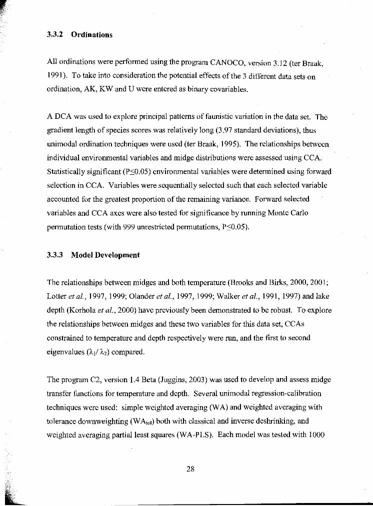
3.3.2 Ordinations

All ordinations were performed using the program CANOCO, version 3.12 (ter Braak,

199 1). To take into consideration the potential effects of the 3 different data sets on

ordination, AK, KW and U were entered as binary covariables.

A DCA was used to explore principal patterns of faunistic variation in the data set. The

gradient length of species scores was relatively long (3.97 standard deviations), thus

unimodal ordination techniques were used (ter Braak, 1995). The relationships between

individual environmental variables and midge distributions were assessed using CCA.

Statistically significant (P50.05) environmental variables were determined using forward

selection in CCA. Variables were sequentially selected such that each selected variable

accounted for the greatest proportion of the remaining variance. Forward selected

variables and CCA axes were also tested for significance by running Monte Carlo

permutation tests (with 999 unrestricted permutations, P50.05).

3.3.3 Model Development

The relationships between midges and both temperature (Brooks and Birks, 2000,2001 ;

Lotter et al., 1997, 1999; Olander et al., 1997, 1999; Walker et al., 199 1, 1997) and lake

depth (Korhola et al., 2000) have previously been demonstrated to be robust. To explore

the relationships between midges and these two variables for this data set, CCAs

constrained to temperature and depth respectively were run, and the first to second

eigenvalues (Al/ h2) compared.

The program C2, version 1.4 Beta (Juggins, 2003) was used to develop and assess midge

transfer fbnctions for temperature and depth. Several unimodal regression-calibration

techniques were used: simple weighted averaging (WA) and weighted averaging with

tolerance downweighting (WAtOr) both with classical and inverse deshrinking, and

weighted averaging partial least squares (WA-PLS). Each model was tested with 1000

bootstrap cycles, and evaluated by means of the bootstrapped co-efficient of

determination (Zboot) and root mean squared error of prediction (RMSEP).

3.4 Results

3.4.1 Faunistic Description

Over 27,000 midge subfossils from 78 taxa were examined. Ranking of taxa by latitude,

temperature and depth (Figs. 3.2-3.4) revealed patterns in the distribution of many taxa.

For the temperature and depth graphs, only the taxa showing relationships with the

variable were included. Abiskomyia, Mesocricotopus, Zalutschia type B, Parakiefferiella

nigra type and Eukiefferiella/Tvetenia were restricted to deep lakes in the colder regions,

the first two taxa being further restricted to only the northernmost lakes. Zalutschia type

A, Corynocera oliveri type and Derotanypus (in low abundances, not graphed) showed a

preference for cold and shallow lakes. Sergentia, commonly interpreted as a cold

indicator (Palmer et al., 2002; Walker, 1 WO), showed little relationship with temperature,

but did show a clear pattern of higher abundances in the deeper lakes. The warm

indicators (Labrundinia, Chaoborus, Pseudochironomus and Glyptotendipes) seemed to

show little correlation with depth. A few of the most common taxa were truly eurytopic

with uniform distributions across latitude, temperature, and depth. These included: other

Tanytarsina, Procladius and other Pentaneurini. Both ceratopogonids and Chaoborus

showed strong preferences for sites below treeline.

Corynocera ambigua and Corynocera oliveri type were mostly restricted to latitudes

north of -60" N. At these latitudes, they were common (found in 44% and 30% of lakes,

respectively) especially in shallow lakes, and often attained high abundances within a

lake (with maximums of 57% and 37% respectively). C. oliveri type was found in the

colder regions, while C. ambigua showed no correlation with temperature.

% a

bund

ance

Figu

re 3

.4 A

chi

rono

mid

dia

gram

for t

he B

erin

gia

trai

ning

set

, with

sel

ect t

axa

rank

ed b

y m

ean

dept

h (s

hallo

w to

dee

p) a

s de

term

ined

by

a c

onst

rain

ed C

CA

. A

ll ta

xon

abun

danc

es a

re p

rese

nted

as

a %

of t

he to

tal i

dent

ifia

ble

chir

onom

ids.

3.4.2 Ordinations

Ordination analyses included 60 taxa, 2 1 environmental variables and 1 14 sites. In order

to determine the extent to which individual environmental variables contributed to

variation, forward selection in CCA was performed. In the initial run (I), AK, KW and U

were entered as covariables, and all variables were selected in the order dictated by

forward selection. Ten environmental variables explained significant proportions

(P50.05) of the explainable variance. In order, these were DEPTH, JTEMP, pH, DOC,

T-ARC, Ca, DIC, TPU, SECCHI and SA (Table 3.2).

With the selection of each variable in forward selection, the relative importance of the

remaining variables is re-evaluated. A variable will decrease in relative importance if it

is correlated with (i.e., explains some of the same variation as) the variables already

selected. Thus, a variable that initially appears important might escape selection, if it is

correlated with variables already selected.

To test the robustness of the variables selected, a different order was forced by selecting

TPU ahead of DEPTH, since both initially explained equal amounts of the variation

(0.1110.66). Run 2 produced similar results: TPU, DEPTH, JTEMP, DIC, Ca, T-ARC,

SECCHI, Mn, DOC and SA. Run 3 was conducted without covariables, and again all

variables were selected in the order dictated by the forward selection procedure. This

produced ten significant variables: T-ARC, DEPTH, JTEMP, DIC, Ca, DOC, TPU,

SECCHI, SO4 and SA. Again a different order was forced (run 4) by selecting the

initially equal (0.1210.78) JTEMP before T-ARC, with similar results: JTEMP, DEPTH,

pH, T-ARC, S04, DOC, TPU, Ca, DIC, SECCHI and SA. Nine variables were

significant across all 4 runs, and were selected for a final CCA (without covariables).

These were DEPTH, JTEMP, T-ARC, TPU, Ca, DIC, DOC, SECCHI and SA.

Patterns in data structure of the final CCA run were compared with those of

correspondence analysis (CA) to explore the impact of the environmental data on species

and site ordination. Similar patterns were observed as assessed both visually, and by

Tab

le 3

.2

Var

ianc

e ex

plai

ned

befo

re a

nd a

fter

for

war

d se

lect

ion

in C

CA

. R

esul

ts a

re p

rese

nted

for:

run

1) C

CA

with

cov

aria

bles

AK

, KW

and

U, a

nd a

ll va

riab

les

sele

cted

in th

e or

der p

rese

nted

; run

2)

CC

A w

ith c

ovar

iabl

es A

K, K

W a

nd U

, TPU

sel

ecte

d fi

rst,

and

all o

ther

var

iabl

es se

lect

ed in

the

orde

r pr

esen

ted;

run

3) C

CA

with

out c

ovar

iabl

es, a

nd a

ll va

riab

les s

elec

ted

in th

e or

der p

rese

nted

; and

run

4) C

CA

with

out c

ovar

iabl

es, J

TE

MP

sele

cted

fir

st, a

nd

all o

ther

var

iabl

es s

elec

ted

in th

e or

der p

rese

nted

.

Cov

aria

bles

AK

, KW

, U

No

cova

riab

les

Var

iabl

e B

efor

e fo

rwar

d A

dded

with

sel

ectio

n V

aria

ble

Bef

ore

forw

ard

Add

ed w

ith s

elec

tion

DE

PTH

0.

1 1

TPU

JT

EM

P SE

CC

HI

DO

C

TPF

T

-AR

C

Ca

W

DIC

*

pH

Fe

CO

ND

T

-AL

P L

-WO

OD

K

M

n S

102

S A

C1

Na

SO4

Sum

of v

aria

nce

expl

aine

d as

a p

erce

nt

Tot

al e

xpla

inab

le v

aria

nce

2 0.

07

T-A

RC

0.

12

JTE

MP

DE

PTH

T

PU

SEC

CH

I D

OC

S A

C

a T

PF

C

ON

D

pH

DIC

C1

M

n Fe

SO

4 T

-AL

P K

L

-WO

OD

N

a S1

02

Sum

of

vari

ance

exp

lain

ed

as a

per

cent

T

otal

exp

lain

able

var

ianc

e T

otal

var

ianc

e 2.

32

Tot

al v

aria

nce

2.32

comparing CA and CCA values for the first 2 axes. Correlation between CA and CCA

species scores of the first axis (r2= 0.92) and second axis (r2=0.47), and site scores for the

first axis (r2=0.96) and second axis (r2=0.67) were good. This confirms that the

environmental variables included in CCA capture the general patterns of species

distribution observed in CA. As such, only CCA is further considered.

Eigenvalues for the first 4 axes of the final CCA account for 18.0% of the species

variance (Table 3.3). Monte Carlo tests (999 unrestricted permutations) confirmed the

significance of all four axes (P=0.001). Relationships between the significant

environmental variables and the individual axes were examined through correlation

coefficients, t-values and interset correlations (Table 3.4). All variables were

significantly correlated with at least the first or second CCA axis (PF0.05). DEPTH

showed a positive correlation with the first axis and negative correlation with the second

axis. JTEMP showed negative correlations with both the first and second axes.

A biplot of the final CCA sample scores shows a good distribution of sites with respect to

both axes (Fig. 3.5). Sites showed clustering by vegetation type with strong segregation

of forest and arctic tundra sites along the temperature gradient. Arctic tundra sites

clustered predominantly in the top right (coldest) quadrant. Forest sites clustered in the

bottom left (warmest) quadrant, and also extended into adjacent quadrants. The majority

of alpine tundra sites fell along the boundary between arctic tundra and forest sites. Sites

with lichen woodland vegetation were interspersed with the forest sites in the top left

(shallowest) quadrant.

The distribution of CCA species scores reflects the environmental preferences of

individual taxa. Clustered near the right end of axis 1 were deep lakes of the colder

regions, and the taxa associated with them (Fig. 3.6): Abiskomyia, Mesocricotopus,

Parakiefferiella nigra and Zalutschia type B. Bordering the shallow northern lakes of the

top quadrants were Derotanypus, Corynocera spp. and Parachironomus. Spanning the

bottom quadrants Einfeldia, Synorthocladius, Stempellina and CyphomellalHarnischia/

Paracladopelma showed preference for deep lakes in the warmer regions. Taxa clustered

Table 3.3 Eigenvalues, taxon-environmental correlations, cumulative % variance and significance of the four axes for the final CCA.

Axis1 h i s 2 Axis3 Axis4 Eigenvalue 0.227 0.090 0.060 0.041 Taxon-environment correlations 0.850 0.794 0.711 0.728 Cumulative % variance

of taxon data 9.8 13.7 16.2 18.0 of taxon-environment relation 42.2 58.9 70.0 77.5

Significance (probability) of axis 0.001 0.001 0.001 0.001 Sum of all unconstrained eigenvalues 2.325 Sum of canonical eigenvalues 0.539

Tab

le 3

.4 C

anon

ical

coe

ffic

ient

s, th

eir

t-va

lues

and

inte

rset

cor

rela

tions

for t

he f

inal

CC

A.

Can

onic

al c

oeff

icie

nts

t-va

lues

In

ters

et c

orre

latio

ns

Axi

s 1

Axi

s 2

Axi

s 3

Axi

s 4

Axi

s 1

Axi

s 2

Axi

s 3

Axi

s 4

Axi

s 1

Axi

s 2

Axi

s 3

Axi

s 4

DE

PT

Ht

0.54

-0

.85

-0.3

3 0.

04

5.35

" -6

.80"

-2

.06"

0.

23

0.42

-0

.50

-0.1

9 0.

21

SA

t 0.

00

0.34

0.

1 1

0.29

0.

01

3.57

" 0.

93

JTE

MP

-0

.38

-0.4

5 -0

.30

-0.2

4 -4

.39"

-4

.19*

-2

.14"

SE

CC

HIt

0.

09

0.69

-0

.13

-0.1

0 0.

8 1

4.74

" -0

.72

Cat

0.

78

0.38

-1

.12

-0.4

4 5.

67"

2.26

" -5

.09"

T

PU

t -0

.06

0.43

-0

.70

-0.6

9 -0

.61

3.66

" -4

.68*

D

OC

t 0.

00

0.4

1 0.

22

0.65

0.

03

4.23

" 1 .

80

DIC

t -0

.90

-0.3

1 0.

41

0.98

-6

.37"

-1

.77

1.81

T

-AR

C

0.44

-0

.06

0.04

-0

.28

5.18

" -0

.58

0.26

"s

igni

fica

nt a

t P50

.05

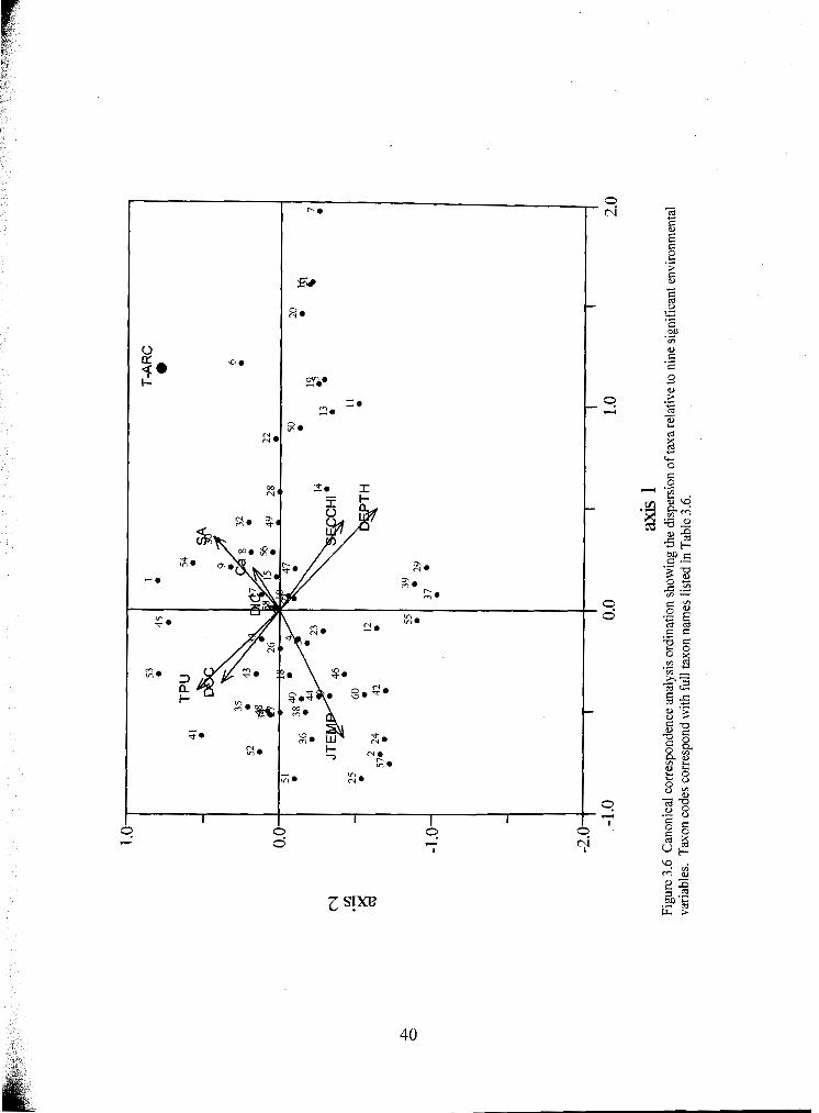
in the central part of the CCA show no distinctive environmental or vegetational

preferences.

3.4.3 Model Development

Depth was the strongest variable overall, as it ranked first or second in all four runs of

forward selection. Mean July air temperature was a close second, and ranked

consistently in the top three variables. CCAs constrained first to depth, and then to

temperature were run, and produced respective eigenvalue ratios of 0.354

(h,/h2=0.1 O5lO.296), and 0.439 (h1/h2=0. 12210.278). WA and WA-PLS models were

constructed using the screened training set (Table 3.5). For depth, WA-PLS with 2 and 3

components produced the strongest models as indicated by their coefficients of

determination and RMSEP7s. The 2 component model was selected as it was the simpler

of the two models (r2bOot=0.43 1, and RMSEP=0.574). For temperature, the WA-PLS

model with 2 components (r2boot=0.507, RMSEP=1.345"C) was again selected over the

WA-PLS model with 3 components.

Taxon specific optima and tolerances were generated using WA (Table 3.6). For depth,

Psectrocladius septentrionalis type generated the shallowest optimum of 3.3 m, while the

deepest was 14.4 m for Abiskomyia. For temperature, the range of optima was relatively

narrow: the lowest optimum of 1 1 .O•‹C was shared by Paracladius and Abiskomyia, and

the highest was 14.4"C for Labrundinia. This narrow range results fiom a short gradient

of mean July air temperatures for the sites (8.6"C to 16.6OC), as well as the tendency of

WA to overestimate low values, and to underestimate high values. Beta values were

generated by the WA-PLS models as coefficients to be used in calculating depth and

temperature estimates.

Table 3.5 A comparison of WA and WA-PLS models for reconstructing a) depth, and b) mean July air temperature.

a) depth

Apparent Bootstrapped

Model 3 RMSE MaxBias 3 RMSEP Max Bias WA inverse 0.454 0.530 1.327 0.346 0.594 1.424

classical 0.454 0.787 0.593 0.354 0.784 0.894 WAtol inverse 0.441 0.536 1.461 0.329 0.618 1.534

classical 0.441 0.808 0.847 0.334 0.858 1 .054 WA-PLS 1 component 0.454 0.530 1.313 0.346 0.596 1.419

2 components 0.634 0.434 1.110 0.431 0.574 1.385 3 components 0.722 0.379 0.91 1 0.434 0.601 1.3 15 4 components 0.769 0.345 0.798 0.424 0.642 1.30 1 5 components 0.788 0.330 0.745 0.404 0.688 1.293

b) mean July air temperature

Avvarent Bootstravved

Model 3 RMSE MaxBias 3 RMSEP Max Bias WA inverse 0.490 1.300 2.686 0.403 1.433 2.893

classical 0.490 1.857 1.952 0.412 1.862 2.413 WAtol inverse 0.438 1.365 2.920 0.341 1.537 3.086

classical 0.438 2.064 2.315 0.349 2.181 2.701 WA-PLS 1 component 0.490 1.300 2.719 0.403 1.432 2.92 1

2 components 0.676 1.036 1.862 0.507 1.345 2.435 3 components 0.744 0.921 1.597 0.504 1.406 2.474 4 components 0.779 0.856 1.529 0.472 1.529 2.641 5 components 0.794 0.827 1.49 1 0.449 1.641 2.758

Tab

le 3

.6 V

alue

s fo

r al

l non

-rar

e ta

xa f

or:

taxo

n oc

curr

ence

(i.e

., pe

rcen

tage

of

121

lake

s in

whi

ch ta

xon

was

pre

sent

), a

nd f

or e

ach

of d

epth

and

mea

n Ju

ly a

ir te

mpe

ratu

re:

taxo

n ra

nge,

WA

opt

imum

(bo

otst

rapp

ed),

WA

tole

ranc

e (b

oots

trat

pped

) and

WA

-PL

S B

eta

coef

fici

ent

(boo

tstr

appe

d).

TE

MPE

RA

TU

RE

D

EPT

H

Tax

on

Tax

on n

ame

occu

rren

ce

T-M

in

T-M

ax

T-O

pt

T-T

o1

WA

PLS

D-M

in

D-M

ax

D-O

pt

D-T

o1

WA

-PL

S

1 D

erot

anyp

us

2 La

brun

dini

a 3

Tr:

Pen

tane

urin

i 4

Pro

clad

ius

5 P

rota

nypu

s 6

Mon

odia

mes

a 7

Abi

skom

yia

8 Corynoneura/Thienernanniella

9 C

rico

topu

s/O

rtho

clad

ius

10 Doithrix/Pseudorthocladius

1 1 E

ukie

fferi

ella

/Tve

teni

a 12

Het

erot

an.v

tars

us

13 H

eter

otri

ssoc

ladi

us

14 H

ydro

baen

us/O

liver

idia

15

Lim

noph

yes

16 M

esoc

rico

topu

s 17

Nan

ocla

dius

18

Ort

hocl

adiin

ae s

p 2

19 P

arac

ladi

us

20 P

arak

ieffe

riel

la n

igra

typ

e 2

1 P

arak

ieffe

riel

la

sp B

22

Par

akie

fferi

ella

tri

quet

ra t

ype

23 P

aram

etri

ocne

mzr

s/P

arap

haen

o.

24 P

sect

rocl

adiu

s (A

llo. &

Mes

o.)

25 P

sect

rocl

adiu

s ca

lcar

atus

typ

e 26

Pse

ctro

clad

ius

(Pse

ctro

clad

ius)

27

Pse

ctro

clad

ius

sept

entr

iona

lis t

y 28

Pse

udos

mitt

ia I

Smitt

ia

29 S

ynor

thoc

ladi

us

30 Z

alut

schi

a ty

pe A

Tab

le 3

.6 c

onti

nued

TE

MPE

RA

TU

RE

D

EPT

H

Tax

on

Tax

on n

ame

occu

rren

ce

T-M

in

T-M

ax

T-O

pt

T-T

o1

WA

PLS

D-M

in

D-M

ax

D-O

pt

D-T

o1

WA

-PL

S co

de

(%)

("C

) ( "

C)

("C

) ("

C)

Bet

a (m

) ( m

) (m

) (m

) I

3 1

Zal

utsc

hia

type

B

14

9.4

14.8

11

.2

1.1

10.7

987

3.0

49.0

12

.3

0.7

4.87

88

32 Z

alut

schi

a za

luts

chic

ola

12

10.2

16

.2

12.7

1.

3 19

.576

2.

0 18

.5

4.4

0.6

-1.2

8516

33

Chi

rono

mus

84

8.

6 16

.6

12.8

1.

9 12

.804

2 0.

8 49

.0

5.2

0.9

1.94

375

34 C

lado

pelm

a 59

9.

0 16

.2

13.2

1.

5 16

.601

8 0.

8 49

.0

4.5

0.9

1.30

735

35 C

rypt

ochi

rono

mus

36

9.

3 16

.0

13.2

1.

6 16

.418

1 0.

8 30

.0

3.7

0.9

-0.2

9642

5 36

Cry

ptot

endi

pes

18

9.3

16.2

13

.3

1.5

16.9

933

1.1

49.0

4.

1 1.

3 0.

3592

71

37 Cyphomella/Harn./Paraclado.

7 10

.6

15.6

13

.1

1.6

20.0

024

3.1

30.0

8.

6 0.

8 4.

5220

1 3 8

Dic

rote

ndip

es

74

8.6

16.6

13

.2

1.6

16.0

121

0.8

49.0

4.

7 1.

2 1.

638

39 E

infe

ldia

8

10.6

16

.2

13.3

1.

7 20

.082

8 4.

0 30

.0

14.3

0.

8 11

.499

8 40

End

ochi

rono

mus

25

9.

3 16

.6

13.5

1.

7 19

.872

8 1.

5 20

.0

5.1

0.8

2.41

458

4 1

Gly

ptot

endi

pes

3 1

9.3

16.2

13

.5

1.7

19.0

994

1.2

49.0

3.

6 0.

8 -0

.483

85

42 Lauterborniella/Zavreliella

5 12

.3

14.8

13

.9

1.0

22.3

987

1.8

30.0

7.

2 1.

2 5.

0242

1 43

Mic

rote

ndip

es

7 1

8.6

16.6

12

.9

1.7

14.9

005

1.1

49.0

4.

3 0.

9 0.

2650

15

44 P

agas

tiel

la

33

9.0

15.3

13

.0

1.5

14.1

285

0.8

49.0

5.

4 1.

4 2.

6734

4 45

Par

achi

rono

mus

25

9.

1 15

.3

12.0

2.

0 5.

6605

7 1.

2 20

.0

. 3.

9 0.

7 -0

.115

844

46 P

arat

endi

pes

9 12

.3

15.6

13

.7

1.0

22.2

21 1

1.

5 49

.0

7.8

1.2

5.48

319

47 P

haen

opse

ctra

flav

ipes

typ

e 20

9.

3 15

.3

12.8

1.

5 14

.870

7 1.

5 49

.0

6.9

1.3

4.11

461

48 P

olyp

edil

um

64

9.2

16.6

13

.3

1.6

17.0

77

0.8

49.0

4.

4 1.

0 0.

8570

96

49 S

erge

ntia

60

8.

6 16

.6

12.1

1.

7 10

.049

5 1.

2 49

.0

7.6

1.2

4.35

293

50 S

tict

ochi

rono

mus

25

9.

3 15

.6

11.4

1.

8 7.

5431

1.

5 49

.0

6.8

0.9

1.20

621

5 1

Pse

udoc

hiro

nom

us

19

10.9

15

.3

13.8

1.

1 21

.146

2 0.

8 30

.0

4.1

1.2

0.03

5675

52

Cla

dota

nyta

rsus

man

cus

type

20

8.

6 16

.2

12.8

1.

9 11

.051

3 0.

8 30

.0

3.4

0.8

-0.3

5566

3 53

Cor

ynoc

era

ambi

gua

34

9.3

15.3

12

.5

1.4

11.8

048

1.5

30.0

3.

5 0.

7 -0

.106

34

54 C

oryn

ocer

a ol

iver

i ty

pe

20

9.3

13.5

11

.8

1.2

6.64

839

0.8

20.3

3.

5 0.

9 -1

.012

17

55 S

tem

pelli

na

13

10.6

16

.0

13.2

1.

2 17

.244

1.

6 30

.0

10.0

1.

0 7.

2159

8 56

Ste

mpe

llin

ella

/Zav

reli

a 69

8.

6 16

.6

12.4

1.

7 12

.362

9 1.

2 49

.0

5.7

1.0

1.70

644

57 T

anyt

arsu

s chi

nyen

sis

9 8.

6 15

.6

13.3

1.

6 16

.879

9 0.

8 13

.2

4.3

0.9

0.86

0915

58

Tan

ytar

sina

- oth

er

100

8.6

16.6

12

.4

1.8

11.3

617

0.8

49.0

5.

6 1.

1 2.

0844

7 59

Cer

atop

ogon

idae

35

10

.6

16.0

13

.5

1.2

17.9

414

0.8

49.0

5.

8 1.

3 2.

8153

7 60

Cha

obor

us

54

8.6

16.6

13

.9

1.5

21.2

15

0.8

20.0

7.

0 0.

7 4.

6028

9

1 T

he b

eta

coef

fici

ents

will

infe

r tra

nsfo

rmed

dep

ths,

whi

ch m

ust b

e co

nver

ted

to re

al d

epth

s by

ebe

ta -1

.

3.5 Discussion

3.5.1 Fauna

All taxa previously included in Canadian temperature models (Palmer et al., 2002;

Walker et al., 199 1, 1997) were also present in this training set. The higher number of

taxonomic groupings here is attributed both to the increased taxonomic resolution of

some groups (e.g., Psectrocladius, Zalutschia, other Tanytarsina; see Appendix I), and to

the presence of a greater number of taxa in this study's larger geographical area. The

most significant additions were 3 species of Corynocera, which were common and often

abundant in this training set, but were entirely absent in the eastern training sets. Among

the taxa included in the other Canadian models, only Pseudodiamesa and Tribelos were

rare in this training set, and excluded from the model.

Co ynocera ambigua has generated discussion for its unusual morphology, and

interesting temporal and spatial distributions (Brodersen and Lindegaard, 1999; Walker et

al., 2003). Distribution in the Beringia training set confirms C. ambigua as a primarily

arcticlsub-arctic taxon, that is rare below -60•‹N (i.e., only 7 head capsules were found in

northern BC). The results of this study also support the conclusion by Brodersen and

Lindegaard (1 999) that temperature is not a limiting factor in the distribution of C.

ambigua. Walker et al. (2003) suggest a Beringian refbgium for this taxon during the last

glacial interval, based on its present distribution and limited flight capabilities.

Some controversy surrounds the taxonomy and identification of Corynocera oliveri type.

A well defined feature of this taxon is the presence of a large surface tooth on the

mandible (Brooks, 2004; Walker, 2000). The median teeth are described as prominent or

on a separate plane, and where the mandibles are absent, C. oliveri type is sometimes

lumped with the similarly described Tanytarsus lugens type (e.g., Brooks and Birks,

2000; R o s h et al., 2003). To further complicate matters, observations on subfossils from

this training set and additional lakes from BC (lakes from Palmer et al., 2002; Walker

and Mathewes, 1988) revealed C. oliveri type mandibles on specimens with different

mentum types (personal observation). For the Beringia training set, the identification of

C. 0hw-i type agrees with available descriptions, but is further restricted to a single

mentum type by a dorso-lateral curvature of the mentum, and is confirmed by the

appearance of a very subtle accessory tooth (or tooth-like shading) often visible between

the median and first lateral teeth, as drawn in Wiederholm (1983; see Appendix 1 for

further details). In the Beringia training set, C. oliveri type resembles C. ambigua in

distribution: it is largely restricted to latitudes north of -60•‹N, is moderately common,

often abundant and is sometimes found in the same lakes as C. ambigua. Although it is

absent from the warmest YukodNWT and Alaska regions, latitude appears to be the

stronger determinant of distribution. Again, its distribution supports the hypothesis of a

Beringia refugium for this taxon.

First reported by Walker and Mathewes (1988), Co ynocera nr. ambigua was identified

at 4 sites in this training set and shows no geographical overlap with the other two

Coynocera spp. The composite records indicate a strongly western/coastal BC

distribution for this taxon. This again supports the suggestion that C. nr ambigua

survived the last glacial interval in a Queen Charlotte Island refugium (Walker and

Mathewes, 1988). Coynocera nr. ambigua was rare in the training set, and excluded

from the model.

3.5.2 Models and Training Set

As inference models get larger in terms of the number of sites, gradient lengths of the

environmental variables typically increase too. The tradeoff in having a training set with

more diverse sites can be larger errors, and weaker r2 values. In a comparison of errors,

this temperature model gives smaller error estimates (RMSEPboot=l 3 5 , RMSEPjack

=1.28) than those for other Canadian models (RMSEPjack= 1.98, Palmer et a/., 2002;

RMSEPjack= 1.87, Rosenberg et al., 2004; RMSEPjack = 2.26, Walker et al., 1997). This

positive result can be partially attributed to a relatively narrow range of mean July air

temperatures in the training set. However, the r2 values (r2boot=~.5 1, r2ja&=~.51) are 2

weaker (r2jack=~.70, Palmer et al., 2002; r jXk=0.73, Rosenberg et al., 2004; r2jaCk=0.88,

Walker et al., 1997), as expected for this larger and more diverse training set. The weak

r2boot (0.43) for the depth model is again expected given the great diversity and range of

depths in the training set. These results were also suggested by the ratios of the first to

second eigenvalues (depth: hd 1 ~ 0 . 3 5 ; temperature: Ill h2=0.44) in the constrained

CCAs. These modest ratios (as compared with hll h2=1. 15 for Walker et a!., 1991)

indicate the importance of multiple variables in explaining the distribution of taxa.

Forward selection in CCA indicates that at least nine environmental variables explained

significant portions of the midge distribution. However, the gap between the variance

explained by the significant environmental variables and the total variance (1.786; Table

3.3) indicates that the distribution of midge taxa is also affected by additional factors not

included in the statistical analyses. For example water temperature (surface and

profundal), lake substrate, sources of food (i.e., within lake flora and fauna) and predators

(i.e., presence of fish) might also contribute significantly to the dispersion of midge taxa.

Where practical, inclusion of additional variables could provide additional information on

distribution of midge taxa.

For the environmental variables that were included, diverse sites that increase the

gradient also increase the chance of capturing the conditions that correspond with past

assemblages. This is especially important in Beringia, as it presents the potential to apply

this model to some of the oldest midge assemblages in the country. To this end, at the

cost of higher errors, future studies might benefit from an even longer gradient of

temperatures. This could be achieved by (1) extending the transect farther north with

sites from the Canadian high arctic, or (2) selecting a different measure of temperature

that better captures the climatic gradient of the transect. The temperature gradient along

the transect is greatest in the winter, suggesting an index that incorporates winter

temperatures, as for example a simple mean annual temperature.

The paucity of quantitative climate data for Beringia makes these models important tools

for data generation. However, some caution is suggested in the interpretation of the

palaeotemperatures and palaeolake-levels derived from these models. Reconstructed

mean July air temperature in particular is constrained by the short gradient (8.6"C to

16.6'C) captured in the training set. The depth gradient is large (<lm to 49 m), but so too

is the error (for example, after correction to untransform the data, an inferred depth of 5

m would have error bars from 2-1 0 m ). As Walker et al. (2003) point out, fluctuations in

water-levels are often too small to be satisfactorily reconstructed. However, atypical

fluctuations of as much as 18m have recently been identified in central Alaska (Abbott et

al., 2000; Barber and Finney, 2000; Bigelow and Edwards, 2001). In regions where large

depth fluctuations have occurred, the midge depth model provides a means to detect and

describe these changes. Of most importance is the usefulness of both models to illustrate

past patterns (i.e., timing, magnitude and direction) of climatic change. Patterns

generated by these models will contribute data that is independent of existing data,

largely based on vegetation records.

In addition to providing data for the models, the training set provides an excellent

database for climate reconstruction by the Modem Analogue Technique. Here again, the

diversity of sites and assemblages captured by the long transect and environmental

gradients is an asset. Where close analogues exist, temperature and depth can be

reconstructed, and insights can be gained into additional elements of the

palaeoenvironment such as vegetation type.

4 A Palaeoclimatic Reconstruction for Antifreeze Pond, Yukon Territory

4.1 Introduction

As scientists work to put current climate change in the context of long tern patterns and

cycles of change, an understanding of past climates is essential. Beringia is an excellent

repository for such palaeoclimatic information. Composed of parts of Yukon, Alaska, the

former Bering Land Bridge and adjacent Siberia, Beringia remained unglaciated

throughout the Quaternary, and contains a wealth of climate sensitive proxies buried in its

sediments.

Early palaeoclimatic studies in Beringia focused largely on pollen, and provide an

understanding of the transition from a cold and dry full glacial to a warmer and wetter

Holocene (Elias, 200 1 a). More recently, additional proxies have proven useful for

addressing higher resolution questions in Beringia and elsewhere. Chironomids, diatoms,

cladocera, loss-on-ignition and other indicators have all contributed to temperature

reconstructions (Battarbee, 2000; Roskn et al., 2003), lake-level reconstructions (Abbott

et al., 2000; Edwards et al., 2000), and the detection of climate reversals (Levesque et al.,

1993). Chironomids (order Diptera) and other midges have been used repeatedly to

produce high resolution temperature reconstructions with errors of less than 2•‹C. No

midge temperature or depth reconstructions exist yet for Beringia.

Antifreeze Pond in southwest Yukon was first cored and the pollen analysed by Rampton

(1969, 1971). Bulk sediment radiocarbon dates obtained by Rampton produced four near

basal dates from 27,100 to 3 1,500 I4c yr BP. These dates are older than most eastern

Beringian cores, which often end with basal dates of late glacial age (for example Abbott

et al., 2000; Bigelow and Edwards, 2001; Hu et al., 1993). While bulk sediment dates

are less reliable than modem AMS dates, these old dates provided the impetus to revisit

and reanalyse Antifreeze Pond.

The aim of this research is to produce a palaeoclimatic record of southwest Yukon by

reconstructing mean July air temperature and depth from 1) recently developed Beringian

midge models, and 2) Modern Analogue Technique used in conjunction with the Beringia

training set.

4.2 Study Area

Antifreeze Pond (62O20.4' N, 140•‹49.2' W; 650 m asl), is situated about 5 km southeast of

the community of Beaver Creek, Yukon, off the east side of the Alaska Highway (Fig.

4.1). This is located in the southeast comer of the Yukon, a mountainous region where

the northwest-southeast trending St. Elias Mountains connect the Coastal Mountains of

Alaska with those of BC.

Protected from the Pacific Ocean by the St. Elias Mountains, Antifreeze Pond is

subjected to a pronounced continental climate (Wahl et al., 1987). Summers are mild

with a mean July air temperature of 13•‹C to 14•‹C (Spatial Climate Analysis Service,

2001 ; Wahl et al., 1987), though daytime highs typically reach 1 8•‹C to 23 "C and can hit

extremes near 30•‹C (Wahl et al., 1987). Winters are long and cold with four months

below -20•‹C, and January the coldest of those at -28•‹C. The region receives 3

approximately 400 mm of precipitation, most falling as rain during the summer months.

The frost-free period extends from late June to mid August, and Antifreeze Pond falls on

the transition between sporadic and extensive discontinuous permafrost. The climate is

hard on vegetation, and Antifreeze Pond is surrounded by stunted black spruce forest and

tussock muskeg, both typical for the region.

Antifreeze Pond is small, with a surface area of approximately 1 ha, and a diameter of

120 m. Late winter measurements gave a maximum lake depth of 1 19 cm, topped by 58

cm of ice. This is approximately equal to a summer depth of 1.7 m. There is no inflow

to the pond; a small outlet exists to the west. Patches of peat are immediately adjacent to

the pond, and the surrounding area is relatively flat. Rampton (197 1) situates Antifreeze

Pond on a moraine deposited by the Mirror Creek glaciation (tentatively equivalent to the

Reid glaciation), and places the maximum extent of the McConnell glaciation (locally

named the Macauley glaciation by Rampton) 6 km to the southeast.

Figure 4.1 Map locating Antifreeze Pond in southwestern Yukon Territory.

4.3 Methods

4.3.1 Field and Laboratory Methods

Antifreeze Pond was cored through the ice in April of 200 1. A modified Livingstone

piston corer was used to retrieve two parallel cores near the deepest part of the pond.

The first and second cores yielded 446 and 5 10 cm of sediment respectively. The cores

were transported to the University of New Brunswick for storage until sampling

The parallel cores were then carefully matched through comparison of their sediments,

and the basal meter from the second core was patched to the first core to form a

continuous 500 cm record. Samples from the patched record were obtained for loss-on-

ignition (LOI), a measure of the organic content of a sample (Dean, 1974; Kurek et al.,

2004).

Up to 3 mL of sediment from each 0.5 cm interval were designated for analysis of

midges. Midges were analyzed at 4 cm intervals, except between 368 and 256 cm where

a preliminary analysis at 8 cm intervals showed chironomid remains to be rare. Midge

processing and identification follows that outlined earlier in this thesis (3.2.2 Midge

Analysis, paragraphs 3 & 4). For statistical significance, a target minimum of 50

identifiable chironomid head capsules per interval was used (Heiri and Lotter, 200 1 ;.

Quinlan and Smol, 200 1). However, concentration of chironomid head capsules varied

greatly throughout the core, and several intervals yielded counts of less than 50 (488.5

cm, 368-256 cm, and 176-148 cm).

4.3.2 Chronology

Twenty six samples were obtained for AMS radiocarbon dating (Table 4.1). All samples

were submitted to the Lawrence Livermore National Laboratory in Livermore, California

for analysis. Dates of <20,000 I4c yr BP were calibrated using CALIB 4.4 (Stuiver and

Reimer, 1993).

Tab

le 4

.1

AM

S ra

dioc

arbo

n da

tes

for

Ant

ifre

eze

Pon

d.

Dep

th (c

m)

Lab

orat

ory

14c ag

e B

P C

alib

rate

d ag

e*

Rel

ativ

e ar

ea u

nder

M

ater

ial d

ated

nu

mbe

r (c

al. y

ears

BP)

pr

obab

ility

dis

trib

utio

n 40

-40.

5 C

AM

S-94

344

2555

=t 30

24

92 -

2596

0.

347

unid

entif

ied

woo

d fr

agm

ents

unid

entif

ied

woo

d fr

agm

ents

unid

entif

ied

woo

d fr

agm

ents

unid

entif

ied

twig

unid

entif

ied

woo

d fr

agm

ents

un

iden

tifie

d w

ood

frag

men

ts

spru

ce a

nd u

nide

ntif

ied

woo

d fr

agm

ents

, 2 s

edge

ach

enes

unid

entif

ied

twig

unid

entif

ied

woo

d fr

agm

ents

unid

entif

ied

woo

d fr

agm

ents

Tab

le 4

.1

cont

inue

d

Dep

th (

cm)

Lab

orat

ory

I4c

~p

Cal

ibra

ted

age*

R

elat

ive

area

und

er

Mat

eria

l dat

ed

num

ber

(cal

. yea

rs B

P)

prob

abili

ty d

istr

ibut

ion

1263

4 - 1

2750

12

789

- 130

07

1305

1 - 1

3.09

8 12

628

- 127

60

1277

6 - 1

3002

13

056

- 130

93

1384

1 - 1

3929

14

069

- 143

75

1461

3 - 1

5357

13

850

- 139

10

1408

0 - 1

4410

14

570

- 154

00

1384

9 - 1

3917

14

079

- 143

95

1459

0 - 1

5384

13

846

- 139

22

1407

6 - 1

4384

14

602

- 153

69

1410

0 - 1

4450

14

530

- 154

40

1387

0 - 1

3889

14

097

- 144

20

1456

0 - 1

5417

14

1 10

- 144

60

14.5

30 -

1543

0 14

120

- 154

40

1435

0 - 1

61 10

17

690

- 216

30

1823

0 - 1

9570

nl

a nl

a

0.24

6 0.

724

0.03

1

0.28

4 0.

699

0.01

8 0.

054

0.52

6 0.

421

0.02

1 0.

482

0.49

7 0.

029

0.50

2 0.

469

0.03

8 0.

516

0.44

6 0.

449

0.55

1

0.00

5 0.

467

0.52

8 0.

426

0.57

4 1 1 1 1 nla

nla

unid

entif

ied

woo

d fr

agm

ents

unid

entif

ied

twig

22.5

Hip

puri

s vu

lgar

is s

eeds

18 E

leoc

hari

s se

eds

40 H

ippu

ris

vulg

aris

see

ds

22.5

Hip

puri

s vu

lgar

is s

eeds

11 E

leoc

hari

s se

eds

1 1.5

Hip

puri

s vu

lgar

is s

eeds

17 E

leoc

hari

s se

eds

unid

entif

ied

twig

un

iden

tifie

d w

ood

frag

men

ts

-230

0 ch

iron

omid

hea

d ca

psul

es

-500

0 ch

iron

omid

hea

d ca

psul

es

5 Po

tam

oget

on f

ruit

ston

es

unid

entif

ied

woo

d fr

agm

ents

+ 2

Car

ex s

eed

coat

s 49

3-49

7 C

AM

S-10

7173

281

70*1

110

nla

nla

unid

entif

ied

woo

d fr

agm

ents

+ 1

Car

ex s

eed

* CA

LIB

4.4

,2 s

igm

a va

lues

(Stu

iver

and

Rei

mer

, 199

3)

** R

ejec

ted

AM

S da

te

Twenty terrestrial and emergent macrofossil samples provided dates for the upper portion

of the core. A date at 114.5 cm was rejected as it was out of line with both the underlying

and older overlying dates. A second reversal occurred in the date at either 50.5 - 5 1 cm

or 58 - 58.5 cm. The age at 58 cm was rejected as this allowed for a more constant rate

of sedimentation. This interval also coincides with the appearance of scmi-terrestrial

chironomids suggestive of fluctuating water levels (see 4.4.1 Midge Stratigraphy) that

could cause re-working of organic matter (Abbott et al., 2000). A tephra layer at 30 cm,

presumed to be the White River Ash, provides the youngest age at 1,250 ' 4 ~ yr BP

(Clague et al., 1995; Richter et al., 1995). A depth-age model for the upper core is

inferred by linear interpolation between the accepted AMS dates (Fig. 4.2).

In the lower core, terrestrial macrofossils were scarce and yielded only three samples

(Table 4.1). A date was also obtained on an aquatic macrofossil. Chironomid head

capsules were recently demonstrated to yield reliable radiocarbon ages (Fallu et al.,

2004), and two chironomid samples from the lower core were picked and dated.

Unfortunately, the lower core ages are problematic and indicate either errors or reversals

in dating (Fig. 4.2). Further, the sedimentation rate in the upper core is variable, and

precludes extrapolation to a basal date.

A date of 43,830 * 8 10 I4c yr BP was obtained on five Potamogeton fruitstones (449 -

450.5 cm). Given the presence of underlying undisturbed laminae (at 490 - 500 cmj, and

given that Potamogeton is an aquatic, the hitstones must have originated in the pond

during the timespan represented by the core. Dates obtained on aquatic macrofossils are

at risk of contamination with old carbon if a I4c reservoir effect exists (Abbott and

Stafford, 1996; Bjorck and Wohlfarth, 2001). At present, Antifreeze Pond is shallow

with no evidence of carbonates or local limestone to suggest such an effect, though past

sources of old carbon are hard to rule out (Hutchinson et al., 2004).

Despite the reliable chironomid dates obtained by Fallu et al. (2004), two factors

predispose the chironomid dates of this study to contamination errors. Firstly, these

samples are older than the Holocene aged samples of Fallu et al. (2004), and thus any

contamination with modern carbon would have a greater effect (i.e., produce a greater

error) on the reported age of the sample. In addition, these chironomid samples have a

greater probability of contamination from modern carbon, as they took longer to pick due

to their larger sizes (-2300 and -5000 chironomid headcapsules compared with an

average of -2000 for Fallu et al.). Despite efforts to maintain a clean work environment,

foreign fibres had to be removed from both samples prior to submission.

Terrestrial macrofossils are the preferred material for radiocarbon dating, as they

generally yield the most reliable dates (Bjorck and Wohlfarth, 2001). However, even the

terrestrial macrofossil dates in the lower core are problematic. The two older dates are on

macrofossils of mixed sources (unidentified wood fragments and Carex seed coats) and

have very large errors (1 110 and 6640 14c yr). In addition a reversal in these two older

terrestrial dates exists. Reversals are often explained by a re-working of older material

into younger sediments (Bjorck and Wohlfarth, 2001), though the older date is supported

by the (admittedly also problematic) aquatic date.

Dates from all three source materials were obtained at -450 cm, and gave a large age

range of -28,000 I4c yr. There is the potential that some of this discrepancy can be

attributed to contamination, as both the chironomid and aquatic samples are at risk of

contamination. Important differences exist between the effects of contamination with

younger and older carbon sources. To give some perspective on these effects, a

comparison was done of the percentage of contamination that would be required to

explain the different dates at 450 cm (Table 4.2). For simplification, all samples were

assumed to be of the same real age, and only modern and dead (i.e., inactive) sources of

carbon contamination were considered. Acceptance of the 15,8 10 I4c yr BP chironomid

date requires that a substantial >90% of the terrestrial and aquatic samples were

contaminated with dead carbon. Acceptance of the 38,O 10 "C yr BP terrestrial

macrofossil date requires significant contamination (5 1 %) of the aquatic sample with

dead carbon. This in turn requires a significant input of dead carbon into the watershed,

as atmospheric exchange with this shallow lake would provide a modernizing influence

on the carbon ratio. Acceptance of the 43,830 I4c yr BP aquatic date, or even of a date

Tab

le 4

.2 A

com

pari

son

of th

e th

eore

tical

con

tam

inat

ion

requ

ired

to p

rodu

ce th

e th

ree

diff

eren

t rad

ioca

rbon

dat

es a

t 450

cm

.

Pote

ntia

l rea

l age

on

t tam

in at

ion'

App

aren

t age

Age

%

C

Fml

Age

%

C

Fm

Age

Fm

15,8

10

100.

00

0.13

97

n!a 0.

00

n/a

15,8

10

0.13

97

15,8

10

6.30

0.

1397

de

ad

93.7

0 0

38,0

10

0.00

88

15,8

10

3.08

0.

1397

de

ad

96.9

2 0

43,8

30

0.00

43

38,0

10

86.7

9 0.

0088

m

oder

n 13

.21

1 15

,810

0.

1397

38

,010

10

0.00

0.

0088

n/

a 0.

00

nla

38,0

10

0.00

88

38,0

10

48.8

6 0.

0088

de

ad

51.1

4 0

43,8

30

0.00

43

43,8

30

86.4

0 0.

0043

m

oder

n 13

.60

1 15

,810

0.

1397

43

,830

99

.55

0.00

43

mod

ern

0.45

1

38,0

10

0.00

88

43,8

30

100.

00

0.00

43

nla

0.00

n/

a 43

,830

0.

0043

infi

nite

86

.03

0 m

oder

n 13

.97

1 15

,810

0.

1397

in

fini

te

99.1

2 0

mod

ern

0.88

1

38,0

10

0.00

88

infi

nite

99

.57

0 m

oder

n 0.

43

1 43

,830

0.

0043

1 Fm

(Fr

actio

n m

oder

n) o

f car

bon

in a

sam

ple

is c

alcu

late

d by

~m

=e

-"

~~

~,

whe

re t

is th

e ag

e of

the

sam

ple

rela

tive

to a

sta

ndar

d of

195

0 T

wo

cont

amin

atio

n so

urce

s are

con

side

red:

dea

d (i

.e.,

inac

tive)

, and

mod

ern

carb

on.

beyond the limits of radiocarbon dating, requires only 14% contamination with modem

carbon in the chironomid sample, and less than 1 % contamination of the terrestrial

sample. If the samples are all of the same age, the discrepancy in dates is most easily

attributed to contamination of the chironomid sample. This comparison supports an age

of >38,OOO 14c yr BP for the lowest section of the core.

Rampton (1 97 1) based his chronology on 10 bulk sediment radiocarbon dates (Table 4.3),

and the correlation of his sediment profile with others in the region. Prominent in the

sediment is a clayey silt layer that Rampton interpreted as loess deposited during the full

glacial. Rampton's date of 13,500 14c yr BP for the upper boundary of the loess provides

a defining date for the retreat of the McConnell glaciation (Fraser and Burn, 1997;

Jackson et al., 199 1). At some localities in the region, a thin layer of tephra, presumed to

be the Dawson tephra, is common near the base of the loess layer and provides a finite

date of -24,000 14c yr BP (Fraser and Burn, 1997; Froese et al., 2002; Rampton, 1969).

Bulk sediment samples in the lower core yielded four dates between -27,000 and

-3 1,000 I4c yr BP, but these were out of order and provide poor chronological control

for the lower core.

Despite efforts to date the lower half of the core, a precise chronology remains elusive.

The available dates are plagued by significant potential for error. Three possible

chronologies are proposed here, though none satisfies all the evidence available, and

other possibilities certainly exist.

Chronology 1. Chronology 1 agrees largely with Rampton, but with one modification.

It infers a hiatus at -375 cm such that the underlying two zones are of interstadial age, the

overlying zone (-375 to -250 cm) is sediment deposited near the end of the 111 glacial

(i.e., early deglaciation), and the peak of the full glacial is absent from the record. This

chronology attributes the two dates at -375 cm to the overlying sediments, and rejects the

chironomid date at -450 cm (1 5,X 10 I4c yr BP), and the terrestrial macrofossil date at

-495 cm (28,170 14c yr BP).

Table 4.3 Bulk sediment radiocarbon dates from Rampton (1971).

Depth (cm)* Laboratory number I4c age BP Material dated

130-135 GSC-1040 5690 5 140 detritus gyttja 173-178 GSC-1242 8710 * 160 detritus gyttja 197-200 GSC-1042 9980 =t 150 i d a 278-283 GSC-1110 13500 =t 300 clayey silt w organic detritus 392-412 GSC-1048 31500 * 700 organic silt 395-404 GSC-1257 28500 5 440 organic silt 417-432 GSC-1198 27100 * 390 organic silt 502-520 GSC-1230 29700 5 700 organic silt

base of adjacent bog GSC-496 > 36000 organic silt

* In order to better correlate Rampton's published depths with those of this thesis, a correction of 110 cm has been subtracted based on the depth of the White River Ash.

I

Chronology 2: This chronology infers a hiatus at -450 cm with the underlying I

I sediments deposited during the interstadial, the overlying sediments deposited during the

end of the full glacial (i.e., early deglaciation), and no sediments captured during the peak

of the full glacial. This chronology accounts for the dating discrepancy at 450 cm, as the

three dates could all be more or less accurate if the older two dates are associated with the

lower zone, and the younger chironomid date with the overlying sediment. The terrestrial I

macrofossil date at -495 cm (28,170 I4c yr BP) is rejected. 1 I

Chronology 3: Chronology 3 infers a continuous record that extends back to the full

glacial. Here, the lowermost three zones represent variation within the full glacial, with

the basal zone (-500 to -450 cm) deposited during the peak of glaciation, and the

overlying two zones (-450 to -250 cm) during deglaciation. The two older dates at -450

cm (38,010 and 43,830 14c yr BP) are rejected.

4.3.3 Data Analysis

For statistical analyses, taxon abundances were calculated as a percent of total

identifiable midges, while for graphing purposes taxon abundances were presented as a

percent of total identifiable chironomids. Percent abundance data for midges were

compiled and graphed using C2 v1.4 Beta (Juggins, 2003). Stratigraphically constrained

zones were delimited with reference to CONISS (Grimm, 1987) in the program ZONE

v1.2 (Juggins, 1991). Data were square root transformed for further analysis.

Intervals from Antifreeze Pond were compared with samples from a Beringia training set

to assess the similarity between assemblages past and present. The Beringia training set

consists of modem samples from 12 1 lakes from Alaska, Yukon, NWT and BC, and is

described earlier in this thesis (3.2 Methods). Similarity was measured as the squared

chord distance between closest analogues, using Modern Analogue Technique (MAT) in

the program C2 v1.4 Beta (Juggins, 2003). First, the self-similarity of modem

assemblages in the training set (excluding rare taxa and outliers, as defined in section

3.3.1 Data Screening) was assessed, and 75% and 95% confidence intervals for these

values determined. Assemblages from Antifreeze Pond (excluding rare taxa, defined as

above with intervals substituted for lakes) were then compared with those of the training

set to determine the closest analogue for each interval. Squared chord distances greater

than the 95% confidence interval were used to define intervals with no analogue, those

less than the 75% confidence interval indicated good analogues, and those in between

indicated weak analogues (Laing et al., 1999).

Data were then entered into the models for inferring mean July air temperatures and depth

that were developed from the Beringia training set earlier in this thesis (see 3.4.3 Model

Development). Mean July air temperatures and depth were also inferred using MAT to

compare intervals with lakes of the Beringia training set. Given the short gradient of

temperatures in the Beringia training set, and the shallowness of Antifreeze Pond, the five

best analogues (versus the standard 10) were used to calculate weighted averages of

temperature and depth. This procedure was followed to ensure the sensitivity of

reconstructions, although it came at the cost of higher sample specific errors.

4.4 Results

4.4.1 Midge Stratigraphy (Fig. 4.3)

Zone AF-1 (497.5-450.5 cm)

This basal zone consists of distinctive and unusual assemblages with a low taxon

richness. CricotopuslOrthocladius dominates, constituting -30-70% of the assemblages;

Sergentia is also prominent at -10-30%. Low abundances of Covynocera oliveri type,

Chironomus, Zalutschia sp A, Procladius, Psectrocladius (Psectrocladius), Tanytarsina -

other (not shown in fig. 4.3) and Covynoneura/Thienemanniella fill out the assemblages.

The organic component in the basal sediments is low, with an average LO1 of 5%. The

assemblages and LO1 throughout this zone are uniform until a sharp transition leads into

zone 2.

Zone AF-2 (450.5-366 cm)

The number of taxa present in zone AF-2 is twice that found in the previous zone. The

formerly dominant CricotopuslOrthocladius almost disappears (-1 %), whereas Sergentia

remains abundant (-10-50%). Corynocera oliveri type increases with peaks of up to

35%. The increased taxon richness is made up of Psectrocladius calcaratus type,

Psectrocladius septentrionalis type and an increase in Chironomini taxa. LOI also

increases to an average of 13%. Like AF-1, the assemblages within this zone are

generally uniform.

Zone AF-3 (366-258 cm)

Chironomids were rare in this zone with samples averaging one chironomidlcm3 (Table

4.4). These exceptionally low counts create unrepresentative percentage data, and so

were omitted from the stratigraphy and reconstructions. LO1 for this zone is the lowest in

the core at about 3%.

Zone AF-4 (258-146 cm)

CricotopuslOrthocladius increases from AF-2 levels to -I%, while the formerly

abundant Sergentia and Corynocera oliveri type are virtually absent. Chironomus

(-32%) and Cryptochironomus (-1 %) are at their maximum abundance in this zone,

while Glyptotendipes (-5%) is entirely restricted to this zone. Some of the taxa found in

zone AF-2 re-appear, for example Psectrocladius (Psectrocladius), Polypedilum, and

Dicrotendipes, while others such as Psectrocladius calcaratus type, Psectrocladius

septentrionalis type and Microtendipes do not. Four semi-terrestrial taxa appear in this

zone: Limnophyes, ParametriocnemuslParaphaenocladius, PseudosmittialSmittia and

Unknown sp 12. The top four intervals of this zone, with low counts (16-27 head

Unknown sp 1 is assumed to be semi-terrestrial based on its strong correlation with semi-terrestrial taxa here, and its co-occurrence with Limnophyes elsewhere (pers. obs.)

Table 4.4 Raw midge data (number of head capsules recovered) for intervals 260 to 360 cm of Antifreeze Pond.

depth (cm) # of head taxa capsules

260 5.0 Tanytarsina - other (3), Chironomus (I), Cricotopus/Orthocladius (1) 264 1.0 Chironomus (1) 272 0.0 280 1.0 Chironomus (1) 288 0.0 296 0.5 Microtendipes (0.5) 312 0.0 320 3.5 Tanytarsina - other (2), Chironomus (OS), Polypedilurn (1) 328 0.0 336 2.0 Tanytarsina -other (2) 344 0.0 352 4.0 Tanytarsina - other (I), Cryptochivonomus (l), chironomidae - unidentified (2) 360 1.0 Procladius (1)

capsules), require caution in their interpretation. The general uniformity of assemblages

through the remainder of this zone shows that counts of 235 head capsules are sufficient

to be statistically representative. LO1 increases somewhat, but remains low at 6%.

Zone AF-5 (146-0 cm)

No taxa dominate this zone, rather the assemblages are composed of a diverse fauna. At

the base of the zone, a peak in Zalutschia type A coincides with the appearance of

Propsilocerus. Following this, there is a synchronous appearance (at 130 cm) of

Psectrocladius calcaratus type, Psectrocladius septentrionalis type, Pagastiella and

Pseudochironomus. Three semi-terrestrial taxa Limnophyes, Parametriocnemusl

Paraphaenocladius and Unknown sp 1 re-appear from 58-30 cm. At 30 cm, the

deposition of the White River Ash further affects the assemblages: Tanytarsus chinyensis

type appears, Psectrocladius septentrionalis type increases, and Pseudochironomus and

Microtendipes decrease. LO1 for the zone begins with a sharp increase to 94% (from 6%

in the previous zone), then plateaus at 78% before dropping again to 42% following the

White River Ash.

4.4.2 Temperature and Depth Reconstructions

The Beringia training set provided adequate analogues (squared chord distance i 17.4)

for the majority of intervals in Antifreeze Pond (Fig. 4.4). The oldest zone (AF-1)

yielded good analogues (squared chord distance <14. I), for d l but one interval. In zones

AF-2 and AF-4, weak analogues (squared chord distance 14.1 to 17.3) dominated. The

intervals with no analogues occurred primarily in AF-2, at the AF-4lAF-5 boundary (late

glacial to Holocene transition), and following the deposition of the White River Ash at 30

cm. This method provides a conservative evaluation of analogues, and confirms that the

Beringia training set (and models derived therefrom) provides a good fit for Antifreeze

Pond.

The WA-PLS and MAT methods yielded very similar patterns in mean July air

66

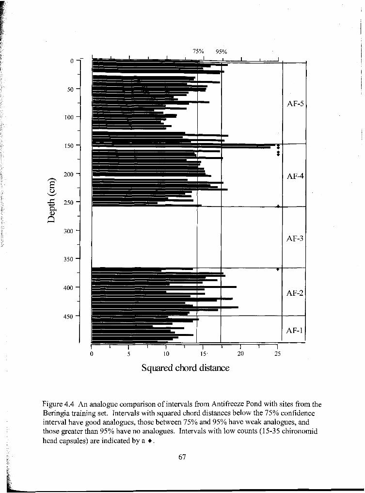
5 10 15. 20

Squared chord distance

AF- 1

Figure 4.4 An analogue comparison of intervals from Antifieeze Pond with sites from the Beringia training set. Intervals with squared chord distances below the 75% confidence interval have good analogues, those between 75% and 95% have weak analogues, and those greater than 95% have no analogues. Intervals with low counts (1 5-35 chironomid head capsules) are indicated by a + .

temperature. Temperatures inferred by the WA-PLS model ranged from 8.9"C to 14.6"C

(Fig. 4.5). The surface sample gave an inferred temperature of 13.OoC, well within the

model error (1.3"C) of the modem temperature obtained from PRISM (13.2"C; Spatial

Climate Analysis Service, 2001). For MAT, the temperature range was narrower at 9.7"C

to 14S0C, and the surface sample lower at 11 3•‹C. Lowess smooths were fitted to both

reconstructions to highlight broad patterns of temperature change.

Changes in lake depth are complicated by the accumulation of sediment over time. With

less accumulated sediment in the past, the overflow (i.e., maximum) depth of Antifreeze

Pond would have been deeper than the present 1.7 m. Inferred depths are compared with

inferred past overflow depths. These overflow depths are estimated by adding sediment

depth to lake depth. For the upper two zones, WA-PLS and MAT inferred very similar

patterns of lake level changes, however for the lower two zones, these patterns differed

(Fig 4.6). For the basal zone (AF-I), the high quality of analogues supports the

reconstruction inferred by MAT. For AF-2, the differences are significant, and it is

unclear which is the more probable reconstruction. Again, lowess smooths were fitted to

the data to highlight the patterns in the lake depth record.

For each zone, the climate as inferred by midges is compared with Rampton's (1 97 1)

climate inferences based on the pollen record. Correlation of the midge and pollen

records was determined primarily by comparison of sediment descriptions for the two

cores (Fig 4.7). Currently, the pollen record is being reanalysed (from the same cores as

the midges) and will allow for better correlation between the midge and vegetation

records.

Zone AF-1 (497.5-450.5 cm)

This basal zone represents the coldest and driest conditions captured by the midges.

Temperatures for this zone inferred by WA-PLS and MAT respectively averaged 3.3"C

and 2.3"C colder than modem. This is the only zone where the MAT inferred depth was

WA-PLS inferred mean July air temperature ( O C ) MAT inferred mean July air temperature ("C)

Figure 4.5 Mean July air temperatures as inferred by WA-PLS and MAT. Lowess smooths (thick lines) are superimposed on the temperature curves (thin lines). Error bars represent sample specific estimated standard errors of prediction. The modern mean July air temperature of 13.2"C is plotted for reference. Intervals with low counts (1 5-35 chironomid head capsules) are indicated by a + .

2 4 6 8 10 12 14 16 18 20 2 4 6 8 10 12 14 16 18 20

WA-PLS inferred depth (m) MAT inkrred depth (m)

-

AF-

AF-

-

A F-

Figure 4.6 Depths as inferred by WA-PLS and MAT. The potential overflow level is plotted for reference. Lowess smooths (thick lines) are superimposed on the depth curves (thin lines). Error bars represent sample specific estimated standard errors of prediction.

Intervals with low counts (1 5-35 chironomid head capsules) are indicated by a + .

mod

ern

tem

pera

ture

s w

et

Mid

ge r

ecor

d

AP

d3

b

AF

-3

-3%

at

leas

t 2-3

•‹C

cold

er th

an m

oder

n

zone

zo

ne

AF

-2

AF

-1

LO1

Pol

len

reco

rd

infe

rred

clim

ate

sedi

men

t

detr

itus

gyttj

a

43

%

-5%

qvtti

a I

shru

b tu

ndra

infe

rred

veg

etat

ion

spru

ce fo

rest

I

clay

ey s

ilts

(slig

htly

org

anic

) se

dge

mos

s tu

ndra

detr

itus

gyttj

a

up to

1 .O

0C co

lder

than

mod

ern

wet

2.3%

to

3.3"

C c

olde

r tha

n m

oder

n ar

id

spru

ce w

oodl

and

AP

d-3a

AP

d-2

AP

d-1

Fig.

4.7

A c

orre

latio

n of

the

mid

ge re

cord

with

Ram

pton

's (

1971

) pol

len

reco

rd. clay

ey s

ilts1

cl

ayey

silt

s w

ith

orga

nic

laye

rs

orga

nic

silts

clay

ey s

ilts

with

or

gani

cs1

orga

nic

silts

sedg

e m

oss

tund

ra

shru

b tu

ndra

fell

field

or

se

dge

mos

s tu

ndra

below the overflow level, at an average of about 4 m. At the base of the zone, the WA-

PLS inferred depth was at overflow (-7 m), and then decreased rapidly to about 2 m.

The good fit of modern analogues for these distinct assemblages prompts further

examination. The group of closest analogues for this zone is dominated by the shallower

tundra lakes (-2 - 4 m) of the Tuktoyaktuk Peninsula (north of treeline). Also, in a

dataset collected by Walker and MacDonald (1 995), four of the taxa from this zone

(Zalutschia, Co vynoneuralThienemanniella, Covynocera and Sergentia) are found to be

most common in shallow tundra lakes.

One of the distinctive features of this zone, is the high percentage of Cricotopusl

Orthocladius (-30-70%). In the Beringia training set, CricotopuslOrthocladius never

exceeds 37%, and the higher abundances are found most often at the northern end of the

transect (Fig. 3.2). Even farther north, abundances of Orthocladius of up to 95% have

been reported on Svalbard, in the high arctic north of Scandinavia (Brooks and Birks,

2004; Birks et al., 2004). Again, these high percentages occur in the shallow lakes (less

than -3 m). This suggests that certain species within this taxon have characteristics

which allow them to withstand the conditions imposed by extreme climates on shallow

lakes. Given the ecology of CricotopuslOrthocladius, Sergentia, Zalutschia sp A,

CorynoneuralThienemanniella and Corynocera oliveri type, the WA-PLS inferred depths

are likely overestimates of the real depths. The location of good analogues at the

northern limit of the transect and the similarity to assemblages of the high arctic, point to

an environment even colder and more extreme than those captured in the Beringia

training set.

Rampton's analysis of the pollen record leads to much the same interpretation. Pollen

spectra indicate that sedge-moss tundra or fell-field covered the landscape, representing a

much colder, and a drier climate than at present. Rampton interprets the low levels of

tree pollen (Picea and Alnus) as indicating long distance transport.

Zone AF-2 (450.5 -366 cm)

The transition to AF-2 is marked by a sharp change in climate. Inferred mean July air

temperatures warmed to modem (MAT) or nearly modem (1 .O•‹C below modern; WA-

PLS). This warming is reflected in the increased productivity, indicated by higher Lo1

and an increase in chironomid richness. Depth for this zone is problematic. WA-PLS

infers a drop in lake level, to below overflow depths of about 2-4 m. In contrast, MAT

infers a strong increase in lake level to depths of 5-8 m that fluctuate broadly at and

above the overflow depth.

Rampton's pollen record reveals a very strong and sudden increase in Betula pollen for

this zone. An increase in shrub birch is indicative of increasing moisture and

temperature, and Rampton interprets a shrub tundra vegetation for this zone. This

supports the MAT inferred increase in lake levels for this zone.

While inferred temperatures approach modem values, midge assemblages and LO1 are

different from modem. This points to environmental and climatic conditions different

from those captured in the Beringia training set.

Zone AF-3 (366-258 cm)

Midges are too rare in this zone to provide temperature and depth reconstructions. The

sediment in AF-3 consists of silt with very little organic matter (LO1 -3%). The near

absence of midges in this zone is most likely caused by low levels of organic matter that

reflect an unproductive environment with little available food. Temperatures at least 2-

3•‹C below modem are inferred by extrapolation from the adjacent zones. Rampton

interprets a cool and dry sedge moss tundra from the pollen record (pollen zone 3a).

Zone AF-4 (258-146 cm; 12,500+ to 9,400 14c BP)

With the re-appearance of midges, temperatures warmed to modem by 12,500 I4c yr BP

(Fig. 4.8). ~ollowing this, there was a rapid deposition of sediment between 230 and 180

cm (12,300 and 12,200 14c yr BP). MAT indicates the possibility that temperatures

surpassed modern by 1 'C at 1 1,500 "C BP. This possible warm peak was followed by a

cold reversal at the transition to zone AF-5. Both reconstructions show a modest cooling

(-1 .O•‹C below modem) from 10,800 I4c BP to 8,500 I4c BP interrupted by a single

warm interval at 9,700 14c BP. This warm interval (148 cm) is possibly an anomaly, as it

is a low midge count interval with high semi-terrestrials that drive the inferred

temperature up. Depth remained at the overflow level, though simultaneous peaks in four

semi-terrestrial taxa are conspicuous, and suggest some fluctuation of water levels and/or

peat development around the lake margin.

Coinciding with the re-appearance of midges, is the appearance of pollen from three

aquatic taxa: Potamogeton, Myriophyllum and Hippuris (pollen zone 3b; Rampton,

197 1). This indicates strong changes in the late glacial limnic environment. In the lower

portion of zone AF-4, a sedge-moss tundra (pollen zone 3b) indicates a climate similar to

that of the full glacial, with shrub tundra not far away. In the upper portion of zone AF-4

(pollen zone 4), Betula peaks again, indicating a change to shrub tundra. Peaks in

Sphagnum and Equisetum spores, and Ericaceae pollen, suggest bog development a r~und

the lake. This shows excellent correlation with the peak in semi-terrestrial chironomids.

The vegetation changes in the upper portion of the core indicate an increase in

precipitation, likely to levels greater than during AF-2.

Zone AF-5 (146-0 cm; 9,400 14c BP to present)

The beginning of the top zone dates to -9,400 I4c BP, and marks the start of the

Holocene record. A remarkable feature of this zone is the increase in organic matter from

6% LO1 in the previous zone to 94% LO1 at the beginning of this zone. Mean July air

temperatures recover from the cold period by -8,000 I4c BP, and modem temperatures

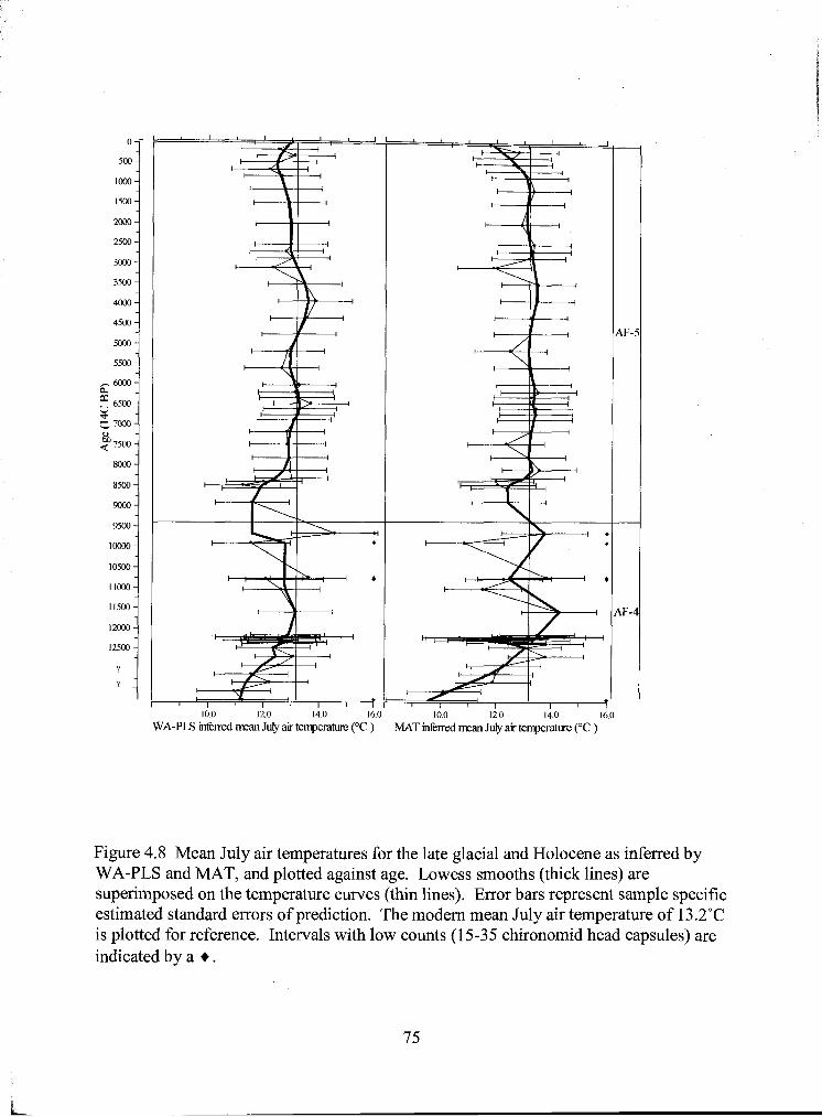
10.0 12.0 14.0 16S

WA-PLS mkrred man July air temperature (OC ) 10.0 12.0 14.0 16.0

MAT mkmd man July air tenperature ("C )

Figure 4.8 Mean July air temperatures for the late glacial and Holocene as inferred by WA-PLS and MAT, and plotted against age. Lowess smooths (thick lines) are superimposed on the temperature curves (thin lines). Error bars represent sample specific estimated standard errors of prediction. The modern mean July air temperature of 13.2"C is plotted for reference. Intervals with low counts (1 5-35 chironomid head capsules) are indicated by a + .

are sustained through the Holocene. Depth is at the overflow level (MAT and WA-PLS),

and remains stable for most the Holocene. Following deposition of the White River Ash

at 1,250 "C BP (Clague et al., 1995; Richter, 1995), inferred temperatures decrease,

especially those inferred by MAT. However, weak analogues for the uppermost intervals

suggest some confounding influence from the tephra. The continued influence of the

tephra in the top intervals is clear from the sustained drop in LOI.

4.5 Discussion and Regional Synthesis

The midge derived zones of Antifreeze Pond are based on robust changes in assemblages,

and coincide with changes in LOI. These sharp transitions imply strong and rapid

changes in the midge environment. The agreement between midge and pollen zones at

several boundaries further demonstrates that many of these changes extended beyond the

limnic environment, and were driven by climate. The vegetation record (pollen and

macrofossils) is currently being re-analyzed, and should help to further resolve the

relationships between the limnic and terrestrial environments, and climate.

A comparison of regional records is complicated by the poor chronological control for

the lower portion of Antifreeze Pond. However, acceptance of any of the near basal dates

makes Antifreeze Pond one of the older lacustrine records in eastern Beringia, as the

majority of lakes yield basal dates of less than 14,000 "C yr BP (for example: Abbott et

al., 2000; Anderson et al., 1994b; Bigelow and Edwards, 200 1 ; Hu et al., 1993; Oswald

et al., 1999). The problems at Antifreeze Pond are not unique: lacustrine and terrestrial

sites that pre-date 14,000 14C yr BP are commonly plagued by poor chronology owing to

gaps in the record, date reversals and/or a lack of finite dates (Anderson and Lozhkin,

2001).

There is good evidence to suggest at least a full glacial and possibly an interstadial age

for some of the lower zones of Antifreeze Pond. A number of full glacial and interstadial

records in east Beringia exist, though they are often plagued by dating problems

(Anderson and Lozhkin, 200 1 ; Schweger and Matthews, 199 1). A selection of some of

the better dated of these records is discussed.

At the Fox permafrost tunnel, Hamilton et al. (1 988) document a record extending from

beyond the limits of radiocarbon dating through the Holocene. Lower and upper units of

perennially frozen silts were deposited as loess during the interstadial and full glacial.

Silt in the lower unit accumulated rapidly, and contains large ice wedges. The base of

this lower silt unit is tentatively assigned a date of 43,000 14c yr BP, though several

infinite dates at the boundary suggest this could be a minimum date. Assemblages above

the base indicate a dry, open meadow with xeric conditions. Separating this lower unit

fkom the upper silt unit is an unconformity characterized by little or no loess deposition,

lenses of buried sod, thaw ponds, and the truncation of ice wedges. This unconforrnity

formed during a period of deep thaw, and defines the Fox Thermal interval (Beget, 1990).

Dates of 33,000 to 30,000 I4c yr BP have been assigned to this interval, though large

errors (>ZOO0 yrs) on a number of the constraining dates, suggest that these ages are

approximate. The development of ponds, and analyses of animal and plant remains,

indicate not only warm, but also mesic conditions. This interval terminates with the onset

of full glacial conditions, represented by the upper silt unit.

A similar climatic record is revealed by magnetic susceptibility analyses on loess sections

in the Goldstream Valley near Fairbanks, Alaska. Beget (1990) and Begkt and Hawkins

(1989) used magnetic susceptibility to track changes in wind intensity, and thus infer

changes in climate. The magnetic susceptibility records at four loess exposures are

correlated with a magnetic susceptibility record from the well dated Fox permafrost

tunnel (Hamilton et al., 1988). The records show a warm (low wind intensity) Holocene,

underlain by a cold (high wind intensity) full glacial, and below that a more variable

interstadial. Within the interstadial, are two warm intervals, interrupted by a cold section.

The chronology at the Fox permafrost tunnel correlates this cold section and the

overlying warm interval with the lower silt unit and overlying Fox Thermal interval.

In the Isabella basin, also located near Fairbanks, Alaska, Matthews (1974) shows a

vegetation response to the full glacial and two part interstadial. The inferred interstadial

pollen record is comprised of two subzones. Matthews interprets the lower of these (zone

Aa, including a bulk sediment date of >3 1,900 "C yr BP, 1-4775) as indicating scattered

spruce in an open sedge dominated vegetation. The late interstadial warming is captured

by zone Ab (including a bulk sediment date of 34,900 * 2950 14c yr BP, 1-3083). Plant

and animal macrofossils point to increases in moisture and temperature. Simultaneous

increases in Picea, Larix, Alnus and Betula (shrub and arboreal macrofossils) indicate

that a higher treeline accompanied the warming. Following this, steppe-like vegetation is

inferred from high levels of Artemisia (to 30%) in the herb zone. From this, Matthews

interprets a cold and arid full glacial climate.

In western Alaska, vegetation records reveal similarities at several sites that include and

pre-date the herb zone: Imuruk Lake (Colinvaux, 1964), Joe Lake (Anderson et al.,

1994a), Kaiyak Lake (Anderson, 1985), Zagoskin Lake (Ager, 2003) and the Kvichak

Peninsula exposure in Bristol Bay (Ager, 1982). Below the herb zone of the full glacial,

the pollen record contains not only herb pollen, but also modest levels of Betula pollen.

In a summary of western Alaskan sites, Ager (2003) characterizes this zone as herb

tundra with birch, and assigns it to the interstadial.

Inferred temperatures for the full glacial are provided by the application of Mutual

Climatic Range (MCR) analysis to beetle remains. Elias (2000,2001b) inferred summer

temperatures for the Last Glacial Maximum in Alaska of 4•‹C colder than modem in

interior Alaska. MCR on beetle remains also estimates winter temperatures as 8•‹C colder

than modern.

Lower Core - Chronology 1

Chronology 1 assumes a hiatus at -375 cm that separates interstadial sediments (AF-1 &

AF-2) from the overlying sediments deposited during the end of the full glacial (i.e., early

deglaciation; AF-3). The peak of the full glacial occurred during the hiatus, and is not

captured by the record. Here, the sequence of distinctive zones provides a basis for

comparing Antifreeze Pond with a selection of regional records.

The sharp transition from a cold and arid zone (AF-1) to a warmer and possibly wetter

zone (AF-2) is a prominent feature in the midge and pollen records at Antifreeze Pond.

This pattern also turns up in the interstadial records fiom Fox permafrost tunnel, the

Goldstream Valley loess and the Isabella basin pollen record (Beg&, 1990; Beg& and

Hawkins, 1989; Hamilton et al., 1988, Matthews, 1974). In addition, the peak in Betula

pollen (45%) during AF-2, correlates with the interstadial herb with birch zone fiom

several pollen records in western Alaska (Ager, 2003). For zone AF-3, a near absence of

midges and very low levels of organic matter could be attributed to rapid sedimentation

during deglaciation. The pollen record during AF-3 is dominated by herbaceous pollen

and correlates well with the herb zone, widespread in eastern Beringia during the full

glacial (Table 2.1).

If chronology 1 is accepted, Antifreeze Pond includes a two part interstadial with a cold

and dry climate (temperatures -2.5 to 3SoC colder than modern) followed by an increase

in moisture and a warming of mean July air temperatures to near modern. No midge

inferred temperatures are available for the full glacial, however extrapolation fiom

adjacent zones points to mean July air temperatures more than 2-3•‹C below modern for

this period.

Lower Core - Chronology 2

Chronology 2 infers a hiatus in the sediment record at -450 cm that separates interstadial

sediments (AF-1) from the overlying sediments deposited during the end of the full

glacial (AF-2 & AF-3).

According to chronology 2, AF-1 is near and possibly beyond the limits of radiocarbon

dating with an upper boundary of 38,000 "C yr BP or older. The lack of finite dates for

this zone, and for this time period at other sites, makes it very difficult to correlate this

zone with other records. It is not clear whether AF-1 is coeval with the earlier cold phase

of the interstadial as for chronology 1 (but why a hiatus during the late interstadial?), or

with the warmer late interstadial (but suggests a very different vegetation and climate

from the regional records). Following the hiatus (-450 cm), a productive environment

(AF-2) is followed by rapid sedimentation (AF-3). This pattern does not appear within

the full glacial in other vegetation records.

If chronology 2 is accepted, the poorly constrained interstadial is arid with mean July air

temperatures 2-3•‹C below modem. Warm and wet conditions much like modem arise

earlier than previously thought at -1 6,000 14c yr BP. However, these near modern

conditions are not continuous through the late glacial: they are punctuated by a zone of

cold and dry conditions with high loess deposition. This would indicate that for the

interstadial and full glacial record at Antifreeze pond, local climatic conditions overrode

any regional trends.

Lower Core - Chronology 3

Chronology 3 assumes a continuous record with the full glacial spanning zones AF-1

through AF-3. For AF-1 and AF-3, the evidence indicates a cold and arid climate, with a

treeless landscape. This agrees with the full glacial climate and conditions inferred from

the herb zone at other sites (Table 2.1). However, these zones are separated by a warm

and wet zone (AF-2) beginning at -16,000 14c yr BP. This fluctuation does not appear in

other herb zone records. The warming inferred here differs from the late glacial warming

at other sites in that it occurs much earlier, and is not sustained through the late glacial.

Acceptance of chronology 3 indicates a full glacial with a cold (mean July air

temperatures 2-3•‹C below modem) and arid climate, punctuated by the appearance of

conditions much like modern. While the cold and arid conditions are synchronous with

regional patterns, the warm and wet interruption is not observed elsewhere and suggests a

strong influence from local climate.

Upper Core

An increase in productivity at the start of AF-4 (shortly before -12,500 "C yr BP), is

shown by increases in LOI, midges and aquatic pollen. This boundary marks the start of

the late glacial. Despite the increased productivity, the telrestrial pollen record shows

little change at this transition. This suggests a higher sensitivity of the limnic

environment to a change in climate. Towards the end of the late glacial, a sharp peak in

Betula pollen indicates an increase in precipitation. In central Alaska, the increase in

birch is dated to -12,000 I4c yr BP at two sites by AMS radiocarbon dating (Bigelow and i Edwards, 2001). Bulk sediment dates at several sites give older dates of -13,500 to

- 12,500 I4c yr BP (Anderson et al., 199413; Bigelow and Edwards, 200 1 ; Hu et al.,

1993), and are likely influenced by a hard water effect. To the east, birch was established

prior to 1 1,300 "C yr BP at Sulphur Lake, southwest Yukon (Lacourse and Gajewski,

2000). At Antifreeze Pond, Rampton's bulk date of -1 0,000 I4c yr BP for the birch peak

is significantly younger than elsewhere, and lacks an explanation. The different timing in

changes to the limnic and terrestrial environments points to a two-step climatic

amelioration.

Midge inferred temperatures began rising before 12,500 I4c yr BP, reached modern by

-12,000 "C yr BP, and possibly peaked about 1 'C above modem (MAT) at 1 1,500 "C yr

BP. Applying MCR to beetle remains, Elias (2000,2001b) finds a similar pattern. The

rapid temperature rise began 12,000 I4c yr BP and peaked 11,000 l4c yr BP at 57•‹C

above modern.

Changing moisture regimes are also indicated by fluctuations in some or all of the four

semi-terrestrial chironomid taxa through the late glacial and Holocene. Their greatest

peak coincides with the rise of birch, and increases in spores of Sphagnum and Equisetum

that point to bog development around the margins of the lake. This further supports an

increase in available moisture, and places a date on the increase of -lO,7OO to -9,500 14c yr BP. Smaller peaks in some of the semi-terrestrial taxa occur at -12,500 to -12,000 14c yr BP and in the Holocene at -3,500 to -1,250 I4c yr BP.

At Birch Lake in central Alaska, Abbott et al. (2000) have used seismic profiles and

multiproxy sedimentary analyses to reconstruct changes in lake levels. From the late

glacial to the Holocene, the dry basin was transformed into a full lake (a change of 18 m)

through a series of fluctuations. The two largest increases in lake level occur from

12,700 to 12,200 I4c yr BP and 10,600 to 10,000 "C yr BP. These dates show excellent

correlation with moisture peaks inferred from the semi-terrestrial chironomids. A third

rise is documented from 8,800 to 8,000 yr BP. Re-examination of the chironomid

record shows a weak peak in two of the semi-terrestrial taxa that is tentatively interpreted

as a moisture signal. Birch Lake attains overflow level by mid-Holocene, and so is

unable to pick up any further moisture peaks (i.e., that suggested by the semi-terrestrial

chironomids from -3,500 to -1,250 14c yr BP).

Using MCR on beetle remains, Elias (2000,2001b) identifies a Younger Dryas cooling

from 1 1,000 to 10,000 I4c yr BP. Midge inferred temperatures also point to a cooling

fi-om 10,800 to 8,500 14c yr BP. While the onset of cooling coincides with the Younger

Dryas, the sustained cooling beyond -1 1,000 14c yr BP suggests that the Younger Dryas

is not the driving force behind this cold period. In addition, this cooling is not reflected

in the pollen record. Even in the chironomid record this cold period is curious, as it

straddles two zones, and a very sharp increase in productivity (i.e., large increases in both

LO1 and chironomid concentration). Closer analysis of these intervals suggests that the

inferred colder temperatures are driven in part by high percentages of Zalutschia type A

(to 18%). In the Beringia training set, Zalutschia type A shows a preference for shallow

lakes in cold regions. Though Propsilocems has no influence on the inferred

temperatures (it was absent in the Beringia training set), its appearance during this cold

peak is noteworthy, as it has only been recorded at two other sites in North America (see

Appendix I). Propsilocerus' distribution at higher latitudes suggests it is a cold indicator

(Szether and Wang, 1996), and it is reported to prefer shallow, eutrophic lakes. This is

consistent with temperature, depth and productivity inferences for Antifreeze Pond

during its appearance in the record. The peaks of these two cold taxa also coincide with

drops or delays in the appearance of several warm taxa (Microtendipes,

Pseudochironomus and Pagastiella).

Temperatures attained modern values by 8,000 "C BP, and were relatively unchanged

through the Holocene. Rampton's (1971) pollen record shows the staggered arrival of

spruce (-8,700 "C BP) and alder (-6,000 "C BP) in the region. These dates agree

generally with dates in central Alaska (Anderson et al., 1994b; Bigelow and Edwards,

200 1 ; Hu et al., 1993).

5 Conclusion

Following the development of the first midge transfer function (Walker et al., 1991),

criticism arose regarding the role temperature plays in directly affecting the distribution

of midge taxa (Ham et al., 1992). Over a decade later, the ecological questions of how

and why midges correlate with summer air temperature remain largely unanswered.

Regardless, multivariate analyses conducted on the Beringia training set confirm that

mean July air temperature is an important variable in determining midge distribution. In

addition, these analyses show that mean July air temperature is strongly correlated with

other variables (i.e., vegetation type, TPU) that also rank high in explaining midge

distribution. This points to a complex, and likely indirect relationship between midges

and mean July air temperature.

Whatever the specifics of the midge temperature relationship, it exists. This is

demonstrated not only by multivariate analyses and model statistics, but also by the

robust temperature reconstructions inferred using midge data. At Antifreeze Pond, both

the WA-PLS model and MAT yielded very similar records of inferred temperature.

These in turn showed excellent correlation with broad patterns in temperatures inferred

locally from pollen, and regionally from vegetation and sediment analyses. Differences

exist in temperatures inferred by midges and terrestrial pollen through the late glacial to

Holocene transition. Reasons for this are not clear; possible explanations include a

higher sensitivity to temperature change by the limnic environment, or a differential

response in midges and terrestrial vegetation to strongly fluctuating temperatures.

The depth midge relationship was explored statistically and through application of a WA-

PLS model and MAT to Antifreeze Pond. Multivariate analyses indicate that depth is the

most important variable in explaining midge distribution in the Beringia training set.

Despite this strong relationship, the WA-PLS model for depth is weaker than that for

temperature as evaluated by the bootstrapped coefficient of determination (r2boot). The

weaker correlation is attributed to the larger gradient of depths included in the model.

Again, the relationship between midges and depth is complex. Though not available for

the Beringia training set, temperature and 0 2 levels at the water sediment interface are

likely important variables that correlate with depth. In addition, depth varies within a

lake depending on the shape of the basin, such that assemblages collected at maximum

depth can be influenced by the lake's bathymetry.

Application of the WA-PLS model and MAT to reconstruct lake depth for Antifreeze

Pond yields mixed results. Inferred WA-PLS and MAT depths for the late glacial and

Holocene show excellent correlation. Further, both show a gradual shallowing consistent

with the inferred accumulation of sediment in the basin during this period. This suggests

a high sensitivity to subtle changes from both methods. Unfortunately, WA-PLS and

MAT show contradictory trends for the lower portion of the core. The trend yielded by

MAT is consistent with moisture changes inferred from the pollen at Antifreeze Pond,

and from other regional records. However, it would be premature to generalize from this

single site that it is the better approach. The discrepancy in results from both the WA-

PLS model and MAT can best be resolved through the application of both approaches to

lakes where the palaeo lake levels are known.

A very interesting correlation was observed here between semi-terrestrial chironomids

and moisture at Antifreeze Pond. Although depth was at overflow through the late

glacial and Holocene, peaks in four semi-terrestrial (i.e., depth or moisture sensitive)

chironomids were conspicuous. Comparison of these peaks with the well documented

palaeohydrology record of Birch Lake (Abbott et al., 2000) in central Alaska showed

remarkable correlation. Again, examination of other sites with well documented

palaeohydrology records is necessary to determine whether this record is unique to

Antifreeze Pond, or whether this approach can be applied elsewhere.

More than three decades after Antifreeze Pond was first cored (Rampton, 1969, 197 l), a

firm chronology is still lacking. New radiocarbon dates support a basal age in the h l l

glacial or interstadial, and suggest several possible chronologies. Resolution of the

chronology is important, as the acceptance of any of the options considered here has

significant implications. If the climatic changes at Antifreeze Pond are synchronous with

those in Alaska, this study provides some of the first quantitative climate data for eastern

Beringia. If, on the other hand, the chronology supports climatic changes that are

asynchronous with regional patterns, this could provide valuable information about the

timing and nature of the McConnell glaciation's retreat.

Improvements to the Beringia training set suggest themselves already: additional lakes

should be added, with particular emphases on expanding the temperature gradient, and

filling out the depth gradient. The promising results yielded by midges at Antifreeze

Pond re-affirm the value of midges as a proxy for climate. The continued application of,

and improvement to, the Beringia training set and its models shows great promise for

significant contributions to our understanding of climate change in eastern Beringia.

REFERENCES

Abbott, M.B., Stafford, T.W., 1996. Radiocarbon geochemistry of modem and ancient arctic lake systems, Baffin Island, Canada. Quaternary Research, 45: 300-3 1 1.

Abbott, M.B., Finney, B.P., Edwards, M.E., Kelts, K.R., 2000. Lake-level reconstructions and paleohydrology of Birch Lake, central Alaska, based on seismic reflection profiles and core transects. Quaternary Research, 53: 154- 166.

Ager, T.A., 1982. Vegetational history of Western Alaska during the Wisconsin glaciation interval and the Holocene. In: Hopkins, D.M., Matthews, J.V., Jr., Schweger, C.E., Young, S.B. (Eds.), Paleoecology of Beringia. Academic Press, New York, pp. 75-93.

Ager, T.A., 2003. Late Quaternary vegetation and climate history of the central Bering Land Bridge from St. Michael Island, western Alaska. Quaternary Research, 60: 19-32.

Alfimov, A.V., Berman, D.I., 2001. Beringian climate during the late Pleistocene and Holocene. Quaternary Science Reviews, 20: 127- 134.

Ammann, B., 2000. Biotic response to rapid climatic changes: introduction to a multidisciplinary study of the Younger Dryas and minor oscillations on an altitudinal transect in the Swiss Alps. Palaeogeography, Palaeoclimatology, Palaeoecology, 159: 191 -20 1.

Anderson, P.M., 1985. Late Quaternary vegetational change in the Kotzebue Sound area, northwestern Alaska. Quaternary Research, 24: 307-32 1.

Anderson, P.M., Brubaker, L.B., 1996. Late Pleistocene and early Holocene pollen records from the southern Brooks Range. In: West, F.H. (Ed.), American Beginnings: The Prehistory and Palaeoecology of Beringia. University of Chicago Press, Chicago, pp. 7 1-82.

Anderson, P.M., Lozhkin, A.V., 2001. The stage 3 interstadial complex (Karginskiilmiddle Wisconsinan interval) of Beringia: variations in paleoenvironrnents and implications for paleoclimatic interpretations. Quaternary Science Reviews, 20: 93- 125.

Anderson, P.M., Bartlein, P.J., Brubaker, L.B., 1994a. Late Quaternary history of tundra vegetation in northwestern Alaska. Quaternary Research, 4 1 : 306-3 15.

Anderson, P.M., Lozhkin, A.V., Eisner, W.R., Kozhevnikova, M.V., Hopkins, D.M., Brubaker, L.B., Colinvaux, P.A., 1994b. Two Late Quaternary pollen records from south-central Alaska. Geographic Physique et Quaternaire, 48: 13 1 - 143.

Barber, V.A., Finney, B.P., 2000. Late Quaternary paleoclimatic reconstructions for interior Alaska based on paleolake-level data and hydrologic models. Journal of Paleolimnology, 24: 29-4 1.

Battarbee, R.W., 2000. Palaeolimnological approaches to climate change, with special regard to the biological record. Quaternary Science Reviews, 19: 107- 124.

Battarbee, R.W., Grytnes, J.-A., Thompson, R., Appleby, P.G., Catalan, J., Korhola, A., Birks, H.J.B., Heegaard, E., Larni, A., 2002. Comparing palaeolimnological and instrumental evidence of climate change for remote mountain lakes over the last 200 years. Journal of Paleolimnology, 28: 1 6 1 - 1 79.

Beget, J.E., 1990. Middle Wisconsinan climate fluctuations recorded in central Alaskan loess. Geographic Physique et Quaternaire, 44: 3- 13.

Beget, J.E., Hawkins, D.B., 1989. Influence of orbital parameters on Pleistocene loess deposition in central Alaska. Nature, 337: 15 1 - 1 53.

Bigelow, N.H., Edwards, M.E., 2001. A 14,000 yr paleoenvironmental record fiom Windmill Lake, central Alaska: late glacial and Holocene vegetation in the Alaska range. Quaternary Science Reviews, 20: 203-2 15.

Birks, H.J.B., Monteith, D.T., Rose, N.L., Jones, V.J., Peglar, S.M., 2004. Recent environmental change and atmospheric contamination on Svalbard as recorded in lake sediments - modern limnology, vegetation, and pollen deposition. Journal of Paleolimnology, 3 1 : 4 1 1-43 1.

Bjorck, S., Wohlfarth, B., 2001. I4c chnostratigraphic techniques in paleolimnology. In: Last, W.M., Smol, J.P. (Eds.), Tracking Environmental Change Using Lake Sediments. Volume 1 : Basin Analysis, Coring, and Chronological Techniques. Kluwer Academic Publishers, Dordrecht, The Netherlands, pp. 205-245.

Bradley, R.S., 1999. Paleoclimatology: Reconstructing Climates of the Quaternary. Academic Press, Toronto.

Brenner, M., Rosenmeier, M.F., Hodell, D.A., Curtis, J.H., 2002. Paleolimnology of the Maya Lowlands. Ancient Mesoamerica, 13 : 141 - 157.

Brodersen, K.P., Lindegaard, C., 1999. Mass occurrence and sporadic distribution of Coynocera ambigua Zetterstedt (Diptera, Chironomidae) in Danish lakes. Neo- and palaeolimnological records. Journal of Paleolimnology, 22: 41 -52.

Brodin, Y.W., Gransberg, M., 1993. Response of insects, especially Chironomidae (Diptera), and mites to 130 years of acidification in a Scottish lake. Hydrobiologia, 250: 201 -2 12.

Brooks, S.J., 2004. Diagnosis of Tanytarsini (Feb. 2004). Unpublished.

Brooks, S.J., Birks, H.J.B., 2000. Chironomid-inferred late-glacial and early-Holocene mean July air temperatures for Kriikenes Lake, western Norway. Journal of Paleolimnology, 23: 77-89.

Brooks, S.J., Birks, H.J.B., 2001. Chironomid-inferred air temperatures from lateglacial and Holocene sites in north-west Europe: progress and problems. Quaternary Science Reviews, 20: 1723- 174 1.

Brooks, S.J., Birks, H.J.B., 2004. The dynamics of Chironomidae (Insecta: Diptera) assemblages in response to environmental change during the past 700 years on Svalbard. Journal of Paleolimnology, 3 1 : 483-498.

Brubaker, L.B., Graumlich, L.J., Anderson, P.M., 1987. An evaluation of statistical techniques for discriminating Picea glauca from Picea mariana pollen in northern Alaska. Canadian Journal of Botany, 63: 61 6-626.

Cannings, R., Scudder, G., 1978. The littoral Chironomidae (Diptera) of saline lakes in central British Columbia. Canadian Journal of Zoology, 56: 1 144- 1 155.

Carter, C., 1977. The recent history of the chironomid fauna of Lough Neagh, from the analysis of remains in sediment cores. Freshwater Biology, 7: 415-423.

Chase, G.E., 2004. Late-glacial chironomid assemblages in northern Maine. M.Sc. thesis, University of Maine, Orono, 36 pp.

Clague, J.J., Evans, S.G., Rampton, V.N., Woodsworth, G.J., 1995. Improved age estimates for the White River and Bridge River tephras, western Canada. Canadian Journal of Earth Sciences, 32: 1 172- 1 179.

Colinvaux, P.A., 1964. The environment of the Bering Land Bridge. Ecological Monographs, 34: 297-329.

Colinvaux, P.A., 1967. Quaternary vegetation history of arctic Alaska. In: Hopkins, D.M. (Ed.), The Bering Land Bridge. Stanford University Press, Stanford, pp. 207-23 1.

Colinvaux, P.A., 1986. Plain thinking on Bering Land Bridge vegetation and mammoth populations. The Quarterly Review of Archaeology, 7: 8-9.

Colinvaux, P.A., West, F.H., 1984. The Beringian ecosystem. The Quarterly Review of Archaeology, 5: 10- 16.

Cranston, P.S., 1995. Introduction. In: Armitage, P.D., Cranston, P.S., Pinder, L.C.V. (Eds.), Chironomidae: the Biology and Ecology of Non-Biting Midges. Chapman and Hall, New York, pp. 1-7.

Cwynar, L.C., 1982. A late-Quaternary vegetation history from Hanging Lake, Northern Yukon. Ecological Monographs, 52: 1-24.

Cwynar, L.C., Levesque, A.J., 1995. Chironomid evidence for late-glacial climatic reversals in Maine. Quaternary Research, 43: 405-4 13.

Cwynar, LC., Ritchie, J.C., 1980. Arctic steppe-tundra: a Yukon perspective. Science, 208: 1375-1377.

Dean, W.E., Jr., 1974. Determination of carbonate and organic matter in calcareous sediments and sedimentary rocks by loss on ignition: comparison with other methods. Journal of Sedimentary Petrology, 44: 242-248.

Dkvai, G., Moldovan, J., 1983. An attempt to trace eutrophication in a shallow lake (Balaton, Hungary) using chironomids. Hydrobiologia, 103: 169- 175.

Edwards, M.E., Arrnbruster, W.S., 1989. A tundra-steppe transition on Kathul Mountain, Alaska, U.S.A. Arctic and Alpine Research, 21: 296-304.

Edwards, M.E., Bigelow, N.H., Finney, B.P., Eisner, W.R., 2000. Records of aquatic pollen and sediment properties as indicators of late-Quaternary Alaskan lake levels. Journal of Paleolimnology, 24: 55-68.

Eisner, W.R., 199 1. Palynological analysis of a peat core from Imnavit Creek, the North Slope, Alaska. Arctic, 44: 279-282.

Eisner, W.R., Colinvaux, P.A., 1992. Late Quaternary pollen records from Oil Lake and Feniak Lake, Alaska, U.S.A. Arctic and Alpine Research, 24: 56-63.

Elias, S.A., 1992. Late Quaternary beetle faunas of southwestern Alaska: evidence of a refugium for mesic and hygrophilous species. Arctic and Alpine Research, 24: 133-144.

Elias, S.A., 2000. Late Pleistocene climates of Beringia, based on analysis of fossil beetles. Quaternary Research, 53: 229-235.

Elias, S.A., 200 1 a. Beringian paleoecology: results from the 1997 workshop. Quaternary Science Reviews, 20: 7- 13.

Elias, S.A., 200 1 b. Mutual climatic range reconstructions of seasonal temperatures based on late Pleistocene fossil beetle assemblages in Eastern Beringia. Quaternary Science Reviews, 20: 77-9 1.

Elias, S.A., Short, S.K., Nelson, C.H., Birks, H.H., 1996. Life and times of the Bering Land Bridge. Nature, 382: 60-63.

Engstrom, D.R., Hansen, B.C.S., Wright, H.E., Jr., 1990. A possible Younger Dryas record in southeastern Alaska. Science, 250: 1383- 1385.

Environment Canada, 1979. Analytical Methods Manual. Inland Waters Directorate, Water Quality Branch, Ottawa, Ontario.

Environment Canada, 1994a. Manual of Analytical Methods: Major Ions and Nutrients, Vol. 1. National Laboratory for Environmental Testing, Canadian Centre for Inland Waters, Burlington, Ontario.

Environment Canada, 1994b. Manual of Analytical Methods: Trace Metals, Vol. 2. National Laboratory for Environmental Testing, Canadian Centre for Inland Waters, Burlington, Ontario.

Fallu, M.-A., Pienitz, R., Walker, I.R., Overpeck, J.T., 2004. AMS 14c dating of tundra lake sediments using chironomid head capsules. Journal of ~a l eo l imno lo~~ , 3 1 : 11-22.

Fraser, T.A., Burn, C.R., 1997. On the nature and origin of "muck" deposits in the Klondike area, Yukon Territory. Canadian Journal of Earth Sciences, 34: 1333- 1344.

Frey, D.G., 1976. Interpretation of Quaternary paleoecology from cladocera and midges, and prognosis regarding usability of other organisms. Canadian Journal of Zoology, 54: 2208-2226.

Froese, D.G., Westgate, J.A., Preece, S.J., Storer, J., 2002. Age and significance of the late Pleistocene Dawson tephra in eastern Beringia. Quaternary Science Reviews, 21: 2137-2142.

Glew, J., 1989. A new trigger mechanism for sediment~samplers. Journal of Paleolimnology, 2: 24 1 -243.

Glew, J., 1991. Miniature gravity corer for recovering short sediment cores. Journal of Paleolimnology, 5: 285-287.

Goetcheus, V.G.; Birks, H.H., 200 1. Full-glacial upland tundra vegetation preserved under tephra in the Beringia National Park, Seward Peninsula, Alaska. Quaternary Science Reviews, 20: 135- 147.

Government of Canada, 2003. Government of Canada climate change website. www.climatechange.gc.ca

Gregory-Eaves, I., Smol, J.P., Finney, B.P., Edwards, M.E., 1999. Diatom-based transfer functions for inferring past climatic and environmental changes in Alaska, U.S.A. Arctic, Antarctic, and Alpine Research, 3 1 : 353-365.

Gregory-Eaves, I., Smol, J.P., Finney, B.P., Lean, D.R.S., Edwards, M.E., 2000. Characteristics and variation in lakes along a north-south transect in Alaska. Archiv fir Hydrobiologie, 147: 193-223.

Grirnm, E., 1987. CONISS: a FORTRAN 77 program for stratigraphically constrained cluster analysis by the method of incremental sum of squares. Computers and Geosciences, 13: 13-35.

Guthrie, R.D., 1968. Paleoecoogy of the large-mammal community in interior Alaska during the late Pleistocene. The American Midland Naturalist, 79: 346-363.

Guthrie, R.D., 1982. Mammals of the mammoth steppe as paleoenvironmental indicators. In: Hopkins, D.M., Matthews, J.V., Jr., Schweger, C.E., Young, S.B. (Eds.), Paleoecology of Beringia. Academic Press, New York, pp. 307-326.

Guthrie, R.D., 1985. Woolly arguments against the mammoth steppe - a new look at the palynological data. The Quarterly Review of Archaeology, 6: 9-1 6.

Guthne, R.D., 1996. Four late Pleistocene large-mammal localities in interior Alaska. In: West, F.H. (Ed.), American Beginnings: The Prehistory and Palaeoecology of Beringia. The University of Chicago Press, Chicago, pp. 1 19- 129.

Guthrie, R.D., 2001. Origin and causes of the mammoth steppe: a story of cloud cover, woolly mammoth tooth pits, buckles, and inside-out Beringia. Quaternary Science Reviews, 20: 549-574.

Hamilton, T.D., Craig, J.L., Sellmann, P.V., 1988. The Fox permafrost tunnel: a late Quaternary geologic record in central Alaska. Geological Society of America Bulletin, 100: 948-969.

Ham, B. J., Warner, B.G., Warwick, W.F., 1992. Aquatic invertebrates and climatic change: a comment on Walker et al. (1 991). Canadian Journal of Fisheries and Aquatic Science, 49: 1274- 1276.

Heinrichs, M.L., Walker, I.R., Mathewes, R.W., Hebda, R., 1999. Holocene chironomid- inferred salinity and paleovegetation reconstruction from Kilpoola Lake, British Columbia. Gkographie Physique et Quatemaire, 53 : 2 1 1-22 1.

Henrikson, L., Olofsson, J.B., Oscarson, H.G., 1982. The impact of acidification on Chironomidae (Diptera) as indicated by subfossil stratification. Hydrobiologia, 86: 223-229.

Heiri, O., Lotter, A.F., 2001. Effect of low count sums on quantitative environmental reconstructions: an example using subfossil chironomids. Journal of Palaeolimnology, 26: 343-350.

Hofinann, W., 1983. Stratigraphy of cladocera and Chironomidae in a core from a shallow north German lake. Hydrobiologia, 103: 235-239.

Hopkins, D.M., 1996. Introduction: the concept of Beringia. In: West, F.H. (Ed.), American Beginnings: The Prehistory and Palaeoecology of Beringia. The University of Chicago Press, Chicago, pp. xvii-xxi.

Hu, F.S., Brubaker, L.B., Anderson, P.M., 1993. A 12,000 year record of vegetation change and soil development from Wien Lake, central Alaska. Canadian Journal ofBotany, 71: 1133-1142.

Hutchinson, I., James, T.S., Reimer, P. J., Bornhold, B.D., Clague, J. J., 2004. Marine and limnic radiocarbon reservoir corrections for studies of late- and postglacial environments in Georgia Basin and Puget Lowlafld, British Columbia, Canada and Washington, USA. Quaternary Research, 6 1 : 193-203.

Hughes, 0. L., 1972. Surficial geology of northern Yukon Territory and northwestern District of Mackenzie, Northwest Territories. Paper 69-36, Geological Survey of Canada, Department of Energy, Mines, and Resources, Ottawa, Ontario.

Jackson, L.E., Jr., Ward, B., Duk-Rodkin, A., 199 1. The last Cordilleran ice sheet in southern Yukon Territory. Geographie Physique et Quaternaire, 45: 341 -354.

Juggins, S., 199 1. ZONE version 1.2. University of Newcastle.

Juggins, S., 2003. C2 version 1.4. University of Newcastle.

Korhola, A., Olander, H., Blom, T., 2000. Cladoceran and chironomid assemblages as quantitative indicators of water depth in subarctic Fennoscandian lakes. Journal of Palaeolimnology, 24: 43-54.

Korhola, A., Birks, H.J.B., Olander, H., Blom, T., 2001. Chironomids, temperature and numerical models: a reply to Seppala. The Holocene, 1 1 : 6 15-622.

Kurek, J., Cwynar, L.C., Spear, R.W., 2004. The 8200 cal yr BP cooling event in eastern North America and the utility of midge analysis for Holocene temperature reconstructions. Quaternary Science Reviews, 23: 627-639.

Lacourse, T., Gajewski, K., 2000. Late Quaternary vegetation history of Sulphur Lake, southwest Yukon Territory, Canada. Arctic, 53: 27-35.

Laing, T.E., Riihland, K.M., Smol, J.P., 1999. Past environmental and climatic changes related to tree-line shifts inferred from fossil diatoms from a lake near the Lena River Delta, Siberia. The Holocene, 9: 547-557.

Laxton, N.F., Bum, C.R., Smith, C.A.S., 1996. Productivity of loessal grasslands in the Kluane Lake region, Yukon Territory, and the beringian "productivity paradox". Arctic, 49: 129- 140.

Lea, P.D., Elias, S.A., Short, S.K., 1991. Stratigraphy and paleoenvironments of Pleistocene nonglacial deposits in the southern Nushagak Lowland, southwestern Alaska, U.S.A. Arctic and Alpine Research, 23: 375-39 1.

Levesque, A.J., Mayle, F.E., Walker, I.R., Cwynar, LC., 1993. The amphi-Atlantic oscillation: a proposed late-glacial climatic event. Quaternary Science Reviews, 12: 629-643.

Lotter, A.F., Birks, H.J.B., Hofmann, W., Marchetto, A., 1997. Modern diatom, cladocera, chironomid, and chrysophyte cyst assemblages as quantitative indicators for the reconstruction of past environmental conditions in the Alps. I. Climate. Journal of Palaeolirnnology, 18: 395-420.

Lotter, A.F., Walker, I.R., Brooks, S.J., Hofmann, W., 1999. An intercontinental comparison of chironomid palaeotemperature inference models: Europe vs North America. Quaternary Science Reviews, 18: 7 17-73 5.

Lotter, A.F., Birks, H.J.B., Eicher, U., Hofmann, W., Schwander, J., Wick, L., 2000. Younger Dryas and Allerod summer temperatures at Gerzensee (Switzerland) inferred from fossil pollen and cladoceran assemblages. Palaeogeography, Palaeoclimatology, Palaeoecology, 159: 349-36 1.

Lozhkin, A.V., Anderson, P.M., Eisner, W.R., Ravako, L.G., Hopkins, D.M., Brubaker, L.B., Colinvaux, P.A., Miller, M.C., 1993. Late Quaternary lacustrine pollen records from southwestern Beringia. Quaternary Research, 39: 3 14-324.

Mathewes, R.W., 1991. Climatic conditions in the western and northern Cordillera during the last glaciation: paleoecological evidence. Gkographie Physique et Quaternaire, 45: 333-339.

Matthews, J.V., Jr., 1974. Wisconsin environment of interior Alaska: pollen and macrofossil analysis of a 27 meter core from the Isabella Basin (Fairbanks, Alaska). Canadian Journal of Earth Sciences, 1 1 : 828-84 1.

Muhs, D.R., Ager, T.A., Beget, J.E., 2001. Vegetation and paleoclimate of the last interglacial period, central Alaska. Quaternary Science Reviews, 20: 4 1-6 1

Natural Resources Canada, 2003. Atlas of Canada. www.atlas.gc.ca/site/index

Nufiez, L., Grosjean, M., Cartajena, I., 2002. Human occupations and climate change in the Puna de Atacama, Chile. Science, 298: 82 1-824.

Olander, H., Korhola, A., Blom, T., 1997. Surface sediment Chironomidae (Insecta: Diptera) distributions along an ecotonal transect in subarctic Fennoscandia: developing a tool for palaeotemperature reconstructions. Journal of Palaeolimnology, 18: 45-59.

Olander, H., Birks, H.J.B., Korhola, A., Blom, T., 1999. An expanded calibration model for inferring lakewater and air temperatures from fossil chironomid assemblages in northern Fennoscandia. The Holocene, 9: 279-294.

Oliver, D.R., Roussel, M.E., 1983. The Insects and Arachnids of Canada, Part 1 1: The General of Larval Midges of Canada, Diptera: Chironomidae. Research Branch, Agriculture Canada, Ottawa.

Oswald, W. W., Brubaker, L.B., Anderson, P.M., 1999. Late Quaternary vegetational history of the Howard Pass area, northwestern Alaska. Canadian Journal of Botany, 77: 570-58 1.

Palmer, S.L., Walker, I.R., Heinrichs, M.L., Hebda, R., Scudder, G., 2002. Postglacial midge community change and Holocene palaeotemperature reconstructions near treeline, southern British Columbia (Canada). Journal of Palaeolimnology, 28: 469-490.

Phillips, D. (Ed.), 1990. The Climates of Canada. Canadian Government Publishing Centre, Environment Canada, 176 pp.

Pienitz, R., Smol, J.P., Birks, H.J.B., 1995. Assessment of freshwater diatoms as quantitative indicators of past climatic change in the Yukon and Northwest Territories, Canada. Journal of Palaeolimnology, 13: 2 1-49.

Pienitz, R., Smol, J.P., Lean, D.R.S., 1997. Physical and chemical limnology of 59 lakes located between the southern Yukon and the Tuktoyaktuk Peninsula, Northwest Territories (Canada). Canadian Journal of Fisheries and Aquatic Science, 54: 330-346.

Porinchu, D.F., MacDonald, G.M., 2003. The use and application of freshwater midges (Chironomidae: Insecta: Diptera) in geographical research. Progress in Physical Geography, 27: 378-422.

Quinlan, R., Smol, J.P., 2001. Setting minimum head capsule abundance and taxa deletion criteria in chironomid-based inference models. Journal of Palaeolimnology, 26: 327-342.

Rampton, V.N., 1969. Pleistocene geology of the Snag-Klutlan area, southwestern Yukon Territory, Canada. Ph.D. thesis, Minnesota University, Minneapolis, 237 PP-

Rampton, V.N., 197 1. Late Quaternary vegetational and climatic history of the Snag- Klutlan area, southwestern Yukon Territory, Canada. Geological Society of America Bulletin, 82: 959-978.

Richter, D.H., Preece, S. J., McGimsey, R.G., Westgate, J.A., 1995. Mount Churchill, Alaska: source of the late Holocene White River Ash. Canadian Journal of Earth Sciences, 32: 74 1-748.

Ritchie, J.C., 1977. The modern and late-Quaternary vegetation of the Campbell- Dolomite Uplands, near Inuvik, N.W.T. Canada. Ecological Monographs, 47: 40 1-423.

Ritchie, J.C., 1984. Past and Present Vegetation of the Far Northwest of Canada. University of Toronto Press, Toronto.

Ritchie, J.C., Cwynar, L.C., 1982. The late Quaternary vegetation of the north Yukon. In: Hopkins, D.M., Matthews, J.V., Jr., Schweger, C.E., Young, S.B. (Eds.), Paleoecology of Beringia. Academic Press, New York, pp. 113-126.

Rosenberg, S.M., Walker, I.R., Mathewes, R.W., Hallett, D.J., 2004. Midge-inferred Holocene climate history of two subalpine lakes in southern British Columbia. The Holocene, 14: 258-271.

Roskn, P., Segerstrom, U., Eriksson, L., Renberg, I., 2003. Do diatom, chironomid, and pollen records consistently infer Holocene July air temperature? A comparison using sediment cores from four alpine lakes in northern Sweden. Arctic, Antarctic, and Alpine Research, 35: 279-290.

Szther, O.A., Wang, X., 1996. Revision of the orthoclad genus Propsilocerus Kieffer (=Tokungayusurika Sasa) (Diptera: Chironomidae). Entomologica Scandinavica, 27: 441-479.

Schwarz, A.G., Wein, R.W., 1997. Threatened dry grasslands in the continental boreal forests of Wood Buffalo National Park. Canadian Journal of Botany, 75: 1363- 1370.

Schweger, C.E., Habgood, T., 1976. The late Pleistocene steppe-tundra in Beringia - a critique. American Quaternary Association Abstracts 4, 80-8 1.

Schweger, C.E., Matthews, J.V., Jr., 1991. The last (Koy-Yukon) interglaciation in the Yukon: comparisons with Holocene and interstadial pollen records. Quaternary International, 10- 12: 85-94.

Schweger, C.E., Matthews, J.V., Jr., Hopkins, D.M., Young, S.B., 1982. Paleoecology of Beringia - a synthesis. In: Hopkins, D.M., Matthews, J.V., Jr., Schweger, C.E., Young, S.B. (Eds.), Paleoecology of Beringia. Academic Press, Toronto, pp. 425- 444.

Seppalii, M., 2001. Unsatisfactory field data in a calibration model for inferring past temperatures from chironomid assemblages in northern Fennoscandia: a comment on Olander, Birks, Korhola and Blom. The Holocene, 1 1 : 6 13-6 15.

Short, S.K., Elias, S.A., Waythomas, C.F., Williams, N.E., 1992. Fossil pollen and insect evidence for postglacial environmental conditions, Nushagak and Holitna Lowland regions, southwest Alaska. Arctic, 45: 38 1-392.

Solem, J.O., Solem, T., Aagaard, K., Hanssen, O., 1997. Colonization and evolution of lakes on the central Norwegian coast following deglaciation and land uplift 9500 to 7000 years BP. Journal of Palaeolimnology, 18: 269-28 1.

Spatial Climate Analysis Service, 2001. PRISM spatial climate layers. Oregon State University.

Stuiver, M., Reimer, P.J., 1993. Extended I4c database and revised CALIB 3.0 14c age calibration program. Radiocarbon, 35: 2 15-230.

ter Braak, C.J.F., 199 1. CANOCO version 3.12. Agricultural Mathematics Group, University of Wageningen, Wageningen, The Netherlands.

ter Braak, C. J.F., 1995. Ordination. In: Jongman, R.H.G., ter Braak, C. J.F., van Tongeren, O.F.R. (Eds.), Data Analysis in Community and Landscape Ecology. Cambridge University Press, Cambridge, pp. 69- 173.

Tokeshi, M., 1995. Life cycles and populations dynamics. In: Armitage, P.D., Cranston, P.S., Pinder, L.C.V. (Eds.), Chironomidae: the Biology and Ecology of Non- Biting Midges. Chapman and Hall, New York, pp. 225-268.

Uutala, A.J., 1990. Chaoborus (Diptera: Chaoboridae) mandibles - paleolimnological indicators of the historical status of fish populations in acid sensitive lakes. Journal of Palaeolimnology, 4: 139- 15 1.

Vereshchagin, N.K., Baryshnikov, G.F., 1982. Paleoecology of the mammoth fauna in the Eurasian arctic. In: Hopkins, D.M., Matthews, J.V., Jr., Schweger, C.E., Young, S.B. (Eds.), Paleoecology of Beringia. Academic Press, New York, pp. 267-279.

Wahl, H.E., Fraser, D.B., Harvey, R.C., Maxwell, J.B., 1987. Climate of Yukon. Environment Canada, Climatological Studies No. 40.

Walker, D.A., Bockheim, J.G., Chapin, F.S., 111, Eugster, W., Nelson, F.E., Ping, C.L., 2001. Calcium-rich tundra, wildlife, and the 'mammoth steppe'. Quaternary Science Reviews, 20: 149- 163.

Walker, I.R., 1988. Late-Quaternary palaeoecology of Chironomidae (Diptera: Insecta) from lake sediments in British Columbia. Ph.D. thesis, Simon Fraser University, Burnaby, 204 pp.

Walker, I.R., 1990. Modern assemblages of arctic and alpine Chironomidae as analogues for late-glacial communities. Hydrobiologia, 214: 223-227.

Walker, I.R., 1995. Chironomids as indicators of past environmental change. In: Arrnitage, P.D., Cranston, P.S., Pinder, L.C.V. (Eds.), The Chironomidae: Biology and Ecology of Non-Biting Midges. Chapman & Hall, pp. 405-422.

Walker, I.R., 2000. The WWW field guide to subfossil midges. www.ouc.bc.ca/eesc/iwalker/wwwguide

Walker, I.R., MacDonald, G.M., 1995. Distributions of Chironomidae (Insecta: Diptera) and other freshwater midges with respect to treeline, Northwest Territories, Canada. Arctic and Alpine Research, 27: 258-263.

Walker, I.R., Mathewes, R.W., 1987. Chironomids, lake trophic status and climate. Quaternary Research, 28: 43 1 -437.

Walker, I.R., Mathewes, R.W., 1988. Late-Quaternary fossil Chironomidae (Diptera) from Hippa Lake, Queen Charlotte Islands, British Columbia, with special reference to Covynocera Zett. The Canadian Entomologist, 120: 739-75 1.

Walker, I.R., Mathewes, R.W., 1989a. Early postglacial chironomid succession in southwestern British Columbia, Canada, and its paleoenvironmental significance. Journal of Palaeolimnology, 2: 1 - 14.

Walker, I.R., Mathewes, R.W., 1989b. Much ado about dead diptera. Journal of Palaeolimnology, 2: 19-22.

Walker, I.R., Smol, J.P., Engstrom, D.R., Birks, H.J.B., 1991. An assessment of Chironomidae as quantitative indicators of past climatic change. Canadian Journal of Fisheries and Aquatic Science, 48: 975-987.

Walker, I.R., Smol, J.P., Birks, H.J.B., 1992. Aquatic invertebrates, climate, scale and statistical hypothesis testing: a response to Hann, Warner, and Warwick. Canadian Journal of Fisheries and Aquatic Science, 49: 1276-1280.

Walker, I.R., Levesque, A.J., Cwynar, L.C., Lotter, A.F., 1997. An expanded surface- water palaeotemperature inference model for use with fossil midges from eastern Canada. Journal of Palaeolimnology, 18: 165- 178.

Walker, I.R., Levesque, A.J., Pienitz, R., Smol, J.P., 2003. Freshwater midges of the Yukon and adjacent Northwest Territories: a new tool for reconstructing Beringian paleoenvironments? Journal of North American Benthological Society, 22: 323-337.

Warner, B.G., Hann, B.J., 1987. Aquatic invertebrates as paleoclimatic indicators? Quaternary Research, 28: 427-430.

Warwick, W.F., 1 989. Chironomids, lake development and climate: a commentary. Journal of Palaeolimnology, 2: 1 5- 1 7.

Wiederholm, T., 1983. Chironomidae of the Holarctic Region. Keys and Diagnoses. Part 1. Larvae. Entomologica Scandinavica, Suppl. 19.

Wiederholm, T., Eriksson, L., 1979. Subfossil chironomids as evidence of eutrophication in Ekoln Bay, central Sweden. Hydrobiologia, 62: 195-208.

Yurtsev, B.A., 2001. The Pleistocene "tundra-steppe" and the productivity paradox: the landscape approach. Quaternary Science Reviews, 20: 165- 174.

APPENDIX

The following bolded taxa constitute a complete list of all taxonomic groups recognized and included in this training set. The primary references used for each taxon are provided. Where identifications emphasized features other than those described in the references, additional notes are provided. Ventromental plates are abbreviated as VP.

Order: Diptera Family: Chironomidae Subfamily: Podonominae Lasiodiamesa (see Wiederholm, 1983)

Subfamily: Tanypodinae Derotanypus (see Wiederholm, 1983) Labrundinia (see Wiederholm, 1983) other Pentaneurini (see Walker, 1988; Wiederholm, 1983) Procladius (see Wiederholm, 1 983) Tanypus (see Wiederholm, 1983)

Subfamily: Diamesinae Diamesa (see Wiederholm, 1983) Potthastia (see Wiederholm, 1983) Protanypus (see Wiederholm, 1983) Pseudodiamesa (see Wiederholm, 1983)

Subfamily: Prodiamesinae Monodiamesa (see Wiederholm, 1983)

Subfamily: Orthocladiinae Abiskomyia (see Wiederholm, 1983) Acamptocladius (see Wiederholm, 1983) BrillidEuryhapsis (see Walker, 2000; Wiederholm, 1983)

Notes: median tooth often absent in half fragments, and mentum of very dark pigmentation.

Cardiocladius (see Wiederholm, 1983) CoryrzoneurdThienemanniella (see Wiederholm, 1 983) Cricotopus/Orthocladius (see Walker, 1988,2000; Wiederholm, 1983)

Notes: a highly variable group with more morphotypes than depicted in the references. Always 6 pairs of lateral teeth, 2nd lateral appressed to the 1" or independent, and VP very reduced and often ending in a dark 'knob'.

Doithrix/Pseudorthocladius (see Walker, 2000) Notes: identified primarily by the paired 4th & 5" pairs of lateral teeth and a slight indent in the edge of the mentum descending from the 5th lateral.

EukiefferielldTvetenia (see Walker, 2000; Wiederholm, 1983) Heterotanytarsus (see Walker, 1988; Wiederholm, 1983) Heterotrissocladius (see Walker, 1 98 8; Wiederholm, 1 983)

Hydrobaenus/Oliveridia (see Walker, 1988,2000; Wiederholm, 1983) Limnophyes (see Walker, 2000; Wiederholm, 1983)

Notes: outer edges of mentum descending from the last laterals are straight and nearly parallel to each other.

Mesocricotopus (see Walker, 2000; Wiederholm, 1983) Metriocnemus (see Wiederholm, 1 983) Nanocladius (see Walker, 1988,2000; Wiederholm, 1983) Orthocladiinae sp 2 (see Walker, 2000)

Notes: mentum similar to Cricotopus/Orthocladius, though taller and narrower with a slight concavity in each half, 6 pairs of lateral teeth though I" pair separated from median tooth only by fine notches, and median tooth sometimes subdivided by additional notches, VP sometimes overlapping lateral teeth.

Paracladius (see Wiederholm, 1983) Notes: whole mentum very pale and broad, single broad median tooth very pale at top edge with weak pigmentation partway down tooth, 6 small pigmented lateral teeth that can be hard to distinguish from each other, last lateral teeth often projecting out at a sharp angle relative to other laterals, VP sometimes overlapping lateral teeth.

Parakiefferiella nigra type (see Walker, 1988; Wiederholm, 1983) Parakiefferiella sp B type (see Walker, 2000; P. cf bathophila in Walker, 1988)

Notes: this taxon is complex, with a gradient of intermediates between two distinctive morphotypes. While the morphotypes at the ends of the spectrum are easily separated, the continuum of intermediates makes it difficult to split this taxon into reliable groups. The co-occurrence in samples of the two morphotypes and intermediates suggests that no ecological information is gained by dividing this complex group, thus they have been lumped. At one end of the spectrum, specimens resemble Parakiefferiella bathophila, with the following features: a single median tooth broader than laterals and rounded or slightly pointed, 1 St pair of lateral teeth appearing either as small accessory teeth attached to the median tooth or as independent teeth resembling the other lateral teeth, an additional 5 pairs of lateral teeth, individual lateral teeth are often hard to distinguish as they are somewhat squished together, and VP bulge out and overlap last lateral teeth. At the other end of the spectrum is the Parakiefferiella sp. B described in Walker (2000) with the following features: median tooth broader than laterals and slightly pointed, weak concavity in each half of the mentum, lSt pair of lateral teeth appearing either as accessory teeth cleaving off the median tooth or as independent teeth resembling the other lateral teeth, an additional 5 pairs of lateral teeth are easily distinguished, the shape of the last laterals is different from other laterals and creates a distinct angle with the other laterals, and VP rarely overlap last laterals.

Parakiefferiella triquetra type (see Walker, 1988; Wiederholm, 1983) Parametriocnemus/Paraphaenocladius (see Wiederholm, 1 98 3) Propsilocerus (see Wiederholm, 1983)

Note: the appearance of over a dozen subfossils of Propsilocerus in Antifreeze Pond is intriguing as this taxon is generally rare, and particularly so in North America. Additional specimens were also found at the same depths in nearby

Eikland Pond (pers. obs.), and subfossils have also been reported from a lake in Maine (Chase, 2004)

Psectrocladius (Allopsectrocladius & Mesopsectrocladius) (see Wiederholm, 1983) Psectrocladius (Psectrocladius) (see Wiederholm, 1 983) Psectrocladius calcaratus type (see Wiederholm, 1 983) Psectrocladius septentrionalis type (see Wiederholm, 1983) Pseudosmittia/Smittia (see Wiederholm, 1983) Rheocricotopus (see Walker, 198 8; Wiederholm, 1983) Symposiocladius lignicola (see Wiederholm, 1983)

Notes: this taxon is synonymous with Orthocladius (Symposiocladius) lignicola in Walker (1988,2000).

Synorthocladius (see Walker, 1988; Wiederholm, 1983) Unknown sp. 1

Notes: this orthoclad is distinctive in its characteristics, and while it shares some similarities with other taxa, it has no exact match in Wiederholm (1 983). The single median tooth is nipple shaped and broader than the laterals, it has 5 lateral teeth with teeth 4 & 5 somewhat paired, and an indentation in the edge of the mentum that descends fiom the 5th lateral. The VPs connect with and extend down from the median tooth; some specimens make it clear that these VPs are on a different plane than the lateral teeth. The edge of mentum continues down below the 5th lateral (and indentation) to give the appearance of a second set of VPs parallel to the first. Mandible with 4 inner teeth. The appearance of this taxon coincided with peaks in Limnophyes, Parametriocnemus/ Paraphaenocladius and Pseudosmittia/Smittia, and suggests that it is semi- terrestrial.

Zalutschia type A (see Walker, 1988) Notes: mental teeth medium to dark pigmentation, each median tooth with small accessory tooth unless worn, median teeth sometimes striated, 5 pairs of lateral teeth identical to each other, last laterals often lower and out of line with other laterals, and mandible with apical and 3 inner teeth all of same colour.

Zalutschia type B Notes: mental teeth medium to dark pigmentation, median teeth asymmetrical with peak on central side of each tooth, 1" lateral reduced and independent, 2nd to 6th laterals identical to each other, mandible with apical and 3 inner teeth all of same colour.

Zalutschia zalutschicola (see Wiederholm, 1983) Notes: median teeth often paler than laterals, 1" pair of lateral teeth reduced and independent, 2nd to 5th pairs identical to each other, 6th pair reduced and sometimes hard to see, and mandible with pale apical tooth and 3 dark inner teeth.

Subfamily: Chironominae Tribe: Chironomini Apedilum (see Wiederholm, 1983) Chironomus (see Walker, 1988; Wiederholm, 1983) Cladopelma (see Walker, 1 98 8; Wiederholm, 1 983) Cryptochironomus (see Walker, 1988; Wiederholm, 1983)

Cvptotendipes (see Walker, 1 988; Wiederholm, 1983) Cyphomella/HarnischidParacladopelma (see Walker, 1 98 8; Wiederholm, 1 983) Dicrotendipes (see Walker, 1988; Wiederholm, 1983) Einfeldia (see Wiederholm, 1983) Endochironomus (see Walker, 1988; Wiederholm, 1983)

Notes: mentum is similar to that of Phaenopsectraflavipes type, Sergentia, Stictochironomus and Tribelos. Tops of teeth darker than the rest of the mentum and median teeth (or rarely, tooth) not much smaller than first laterals. VP differ from the usual 'fan' (or 'triangle') shaped Chironomini VP: the bottom portion of the 'fan' much reduced or absent giving the VP a somewhat 'bar' shaped appearance; the ends of the VP furthest from the mentum often appear rounded. On the VP, upper and lower bands of striations separated by a very small gap, with striations often curving away from mentum near upper margin of VP. Mandibles usually with 3 inner teeth.

Glyptotendipes (see Walker, 1 98 8; Wiederholm, 1 983) Notes: a highly variable group, mentum broad or narrow, with single median tooth notched or simple, 6 pairs of lateral teeth, and VP with striations and ridges along top margin. This taxon also includes specimens originally identified as 'Dicrotendipes/Einfeldia/Glyptotendipes' in the YukonINWT dataset (Walker et al., 2003).

LauterborniellaJZavreliella (see Walker, 1988; Wiederholm, 1983) Microtendipes (see Walker, 1988; Wiederholm, 1983)

Notes: a tiny median tooth occasionally visible between dominant pale median teeth.

Nilothauma (see Walker, 1988; Wiederholm, 1983) Pagastiella (see Walker, 1988; Wiederholm, 1983) Parachironomus (see Walker, 1988; Wiederholm, 1983) Paralauterborniella (see Walker, 1988; Wiederholm, 1983) Paratendipes (see Walker, 1 988; Wiederholm, 1 983) Phaenopsectraflavipes type (see Walker, 1988,2000; Wiederholm, 1983)

Notes: Mentum narrower and usually darker than the similar taxa Endochironomus, Sergentia, Stictochironornus and Tribelos. VP with upper and lower bands of striations separated by a small gap, upper band of striations extends to upper margin of VP. A small indent appears in the VP where it is joined by the bottom edge of the mentum. Mandible with 3 inner teeth.

Polypedilum (see Walker, 1988; Wiederholm, 1983) Sergentia (see Walker, 1 98 8; Wiederholm, 1 983)

Notes: VP with two bands of striations separated by a gap: striations near the upper margin appear as paired ticks while lower band of striation appears more 'normal' (i.e., evenly spaced striae). Median teeth shorter but not much narrower than 1" laterals. Mandible with 4 inner teeth. Compare this taxon with Endochironomus, Phaenopsectrajlavipes type, Stictochironomus and Tribelos.

Stictochironomus (see Walker, 1988; Wiederholm, 1983) Notes: similar to Endochironomus, Phaenopsectrajlavipes type, Sergentia and Tribelos. Median teeth shorter and narrower than all other laterals. Median and lSt laterals of a squared shape (i.e., tops flat, not pointed). Upper part of VP with

no striations; a lower band of striation may be present. Mandible with 3 inner teeth.

Tribelos (see Walker, 1988; Wiederholm, 1983) notes: similar to Endochironomus, Phaenopsectraflavipes type, Sergentia and Stictochironomus. VP with upper and lower bands of striations; upper band does not extend to upper margin of VP (compare with Phaenopsectraflavipes). Mandible with 3 inner teeth.

Xenochironomus (see Wiederholm, 1983)

Tribe: Pseudochironomini Pseudochironomus (see Walker, 1988; Wiederholm, 1983)

Tribe: Tanytarsini Cladotanytarsus mancus type (see Brooks, 2004; Walker, 2000) Corynocera ambigua (see Walker, 2000; Wiederholm, 1983)

Notes: simple mentum with only 5 teeth, median and first pair of lateral teeth on separate plane from 2nd laterals, dorso-lateral curvature of mentum causes 2nd laterals to directly overlap 1" laterals, antennal pedestal elongate with no projection, and mandible with no visible teeth.

Corynocera nr. ambigua (see Walker, 1988,2000) Notes: mentum often very worn and with hard (or impossible) to distinguish teeth, mentum narrower than other Tanytarsini (resembling other Corynocera spp) and often dark, antennal pedestal elongate with small very blunt projection, and mandible with indistinct teeth.

Corynocera oliveri type (see Brooks, 2004; Walker, 2000; Wiederholm, 1983) Notes: an apparent dorso-lateral curvature to mentum (such that middle 3 teeth are never in focus at the same time as outer laterals), median tooth at least as wide as or often wider than first pair of laterals, first pair of lateral teeth taller and wider than other laterals and on the same plane as median tooth, a tiny and subtle accessory tooth (or tooth-like shading) between median and first laterals, 2nd to 5th pairs of laterals not on the same plane as the median trio and often squished together (i.e., overlapping), antennal pedestals elongate with no projection, and mandible with large surface tooth obscuring the inner teeth.

Identification keys for this taxon have relied heavily on the mandible (Brooks, 2004; Walker, 2000). This has created problems, as a survey of specimens from BC lakes (in addition to the Beringia training set) shows that more than one mentum type has a mandible matching the description for C. oliveri type. For this thesis, specimens were identified based on the above description of the mentum, and were confirmed (but not identified) by the mandible. The description of C. oliveri type given here is also consistent with specimens from Russia in the reference collection at University of New Brunswick, Canada (pers. obs).

Rheotanytarsus (see Wiederholm, 1983) Stempellina (see Walker, 1988; Wiederholm, 1983) Stempellinella/Zavrelia (see Walker, 1 98 8; Wiederholm, 1 98 3) Tanytarsus chinyensis (see Brooks, 2004; Walker, 2000)

Tanytarsina other (see Brooks, 2004; Walker, 2000; Wiederholm, 1983) Notes: undifferentiated Tanytarsina not belonging to any of the above listed groups.

Family: Ceratopogonidae (see Walker, 2000)

Family: Chaoboridae (see Uutala, 1990)