Padova, 25 novembre 2009

Padova, 25 novembre 2009

Omar Codemo

Senior Product Engineer

Application Engineering Dept.

e-mail: [email protected]

Algoritmi di calibrazione per telecamere

2

Global Footprint

� Place: Monopoli, Italy� Activity: R&D, Manufacturing� Employees: 225� Area: 7,398 sqm

� Place: Columbia, USA� Activity: R&D, Manufacturing� Employees: 36� Area: 4,325 sqm

� Place: Marseilles, France� Activity: R&D� Employees: 10� Area: 180 sqm

� Place: Treviso, Italy� Activity: R&D, Manufacturing� Employees: 65� Area: 1,500 sqm

MAIN OFFICE� Monopoli, Italy

BRANCH OFFICE� Norway

REP OFFICES� Roma, italy� Switzerland� China� Korea

MAIN OFFICE� Treviso, Italy

R&D LAB� Palermo, Italy

REP OFFICE� China

MAIN OFFICE� Columbia, USA

REP OFFICES� Chicago� Brasil� UK� Italy� Spain� Unghery� Poland� China� Taiwan� Australia

MAIN OFFICE� Marsiglia, France

GLOBAL LOCATIONS

3

MER MEC Group in Numbers

R & D

� 72 main clients in 35 countries worldwide

� 41 unique measuring systems in 6 distinct product families

� 8 Integrated diagnostic vehicles manufactured & sold worldwide

� 350,000 km of line measured by MER MEC Group’s customers

� 436 measuring systems sold worldwide

DIAGNOSTICS

�2,100 km of line equipped with SSC SCMT signaling systems

�SSC (1426 km)

• 1083 LEU

• 1083 Transponders

• 212 Transponder Tags

�SCMT (667 km)

• 100 boxes

• 508 LEU

• 3673 Eurobalise

�2000 entrance in signaling market with a 4 year time to market.

SIGNALLING

�Measuring Services

• 2 Hi-Rail diagnostic vehicles with variable gauge capability

• 1 measuring carriage for use on standard gauge rail lines

• 5 market segments served (Metro, Light Rail, Ordinary Rail, High-Speed, Heavy-Haul)

• Integrated services for data acquisition, analysis and maintenance planning

ADVANCED SERVICES

� 17 main clients in 8 countries worldwide

� 3 industrial sectors served: “Long Products”, “Ring Rollings” and “Large Open-die Forgings”

� 35 Systems installed

IRON & STEEL INDUSTRY

� 154 people involved in R&D

� MUIR authorized research laboratory since 2001

� 15% of revenues invested annually in R&D

� 14 new products commercially launched between 2004-2007

Algoritmi di calibrazione per telecamere 4

Definizione del problema

L’uso di telecamere per l’osservazione di una scena richiede l’uso di obiettivi costituiti da un insieme di lenti.

L’uso di tali lenti introduce una distorsione che bisogna compensare prima di poter procedere ad una qualsiasi misurazione.

Inoltre si osserva una scena 3D tramite un sensore (CCD) che produce un’immagine 2D. Questo porta all’introduzione di una mappatura dettaproiezione prospettica:

DIDS 23 ⊂→⊂Infine il frame grabber può introdurre distorsioni (line jitter, fattori di scala).


Distorsione delle lentiDistorsioni non lineare

Le distorsioni introdotte dalle lenti sono tipicamente non lineari. Si possono suddividere in:

⟩ radiale;

⟩ altre distorsioni delle lenti;

La distorsione radiale sposta i punti fuori dal centro ottico (Barrel o Pincushion) ed è causata principalmente da deviazioni dei raggi ai bordidella lente:

La distorsione delle lenti si può scomporre principalmente in:

⟩ Radiale (dr);

⟩ Tangenziale (dt).


Riassunto tipi di distorsione

Le seguenti distorsioni vanno compensate tramite un processo detto:

CALIBRAZIONE(o Camera resectioning)


Proiezione prospetticaDistorsione lineare

La proiezione prospettica non rispetta distanze e angoli perciò può essere considerata come una forma di distorsione. Tale distorsione si può esprimere tramite una matrice:

Z

fXx =

Zy

fY=

=

≈

Z

Y

X

f

f

Z

fY

fX

y

x

100

00

00

1


Proiezione prospetticaProprietà

1. La dimensione di un oggetto diminuisce all’allontanarsi dal centro di proiezione;

2. La dimensione della proiezione orizzontale diminuisce al ruotare dell’oggetto;

3. Preserva le rette;

4. Sono possibili più punti di fuga;


Pinhole camera model

Il modello Pinhole è molto semplice ed è costituito da una rototraslazione di un corporigido seguita da una proiezione prospettica.

Altre distorsioni a parte la proiezione prospettica (es. quelle delle lenti) non sonomodellizzate. Nonostante ciò è una buona approssimazione.

Dette [xi,yi,zi]T le coordinate di un punto della scena e [ui,vi] T le appropriate coordinate del punto corrispondente sull’immagine si hanno le coordinate intemedie :

È necessaria una ulteriore trasformazione per ottenere le coordinate immagine:

=

i

i~

i

~

i

y

x

v

u

iz

f

+

=

0

0

i

~

V

i

~

U

i

i

v

u

vD

uDv

uDove (u0,v0) tengono conto dello scostamento dell'origine e (Du,Dv) sono fattori di conversione tra le unità di misura del mondo e quelle immagine, e tengono conto dei diversi fattori di scala.



Modificando la scrittura della prima equazione (aggiungengo un vincolo esplicito) la si può rappresentare in forma di sistema :

Dove la matrice A è una matrice triangonale superiore, definita con 5 parametri.

=

i

i

i

z

y

x

Av

u

i

i

λλλ

=

=100

0

100tan2

0

tan2

0

0

0

0

vk

ukk

vH

ukW

A v

u

v

u γ

γ

α

α



Usando le coordinate omogenee:

Dove in molti casi si sottointende λ (dopotutto le coordinate omogenee sono definite a meno di un coefficiente di proporzionalità), e Π0 è una semplice matrice usata per sottointendere la quarta coordinata omogenea (W) non usata in questa trasformazione.

Definiamo la matrice per tener conto della rototraslazione. Da cui:

Π=

11

0i

i

i

i

i

Z

Y

X

Av

u

λ

[ ]0tRE =

=

=

11i

i

i

i

i

i

i

i

Z

Y

X

PZ

Y

X

AEv

u

λλλ


Parametri intrinseci ed estrinseci

Durante la calibrazione un bersaglio fornisce la corrispondenza tra i punti dell’immagine e quelli dello spazio.

Con la calibrazione si identifica la distanza focale f e il punto principale (X0,Y0) T. Tali parametri sono legati all’ottica e sono detti parametri intrinseci.

Il bersaglio non si può posizionare in modo perfetto allora si devono identificare anche le relazioni tra le coordinate della telecamera e quelle del bersaglio. Tali parametri sono detti parametri estrinseci.

Oltre a questi ci sono un fattore di scala che tiene conto del ricampionamento a livello di frame grabber e delle serie di potenze per modellare le distorsioni


Parametri intrinseci ed estrinseci

Ponendo Zi=0 per ogni i si ottiene:

=

=

111 76

43

10

i

i

i

i

Z

Y

X

i

i

Y

X

HY

X

Trr

Trr

Trr

v

u

λ

=

=

111 76

43

10~

~

i

i

i

i

Z

Y

X

i

i

Y

X

KY

X

Trr

Trr

Trr

v

u

λ

Indicando con (ui,vi ) le coordinate immagine normalizzate:~ ~


Calibrazione a forza bruta

Banalmente la calibrazione può essere fatta creando relazione tra due matrici di punti (scena ed immagine) ed andando ad interpolare nel caso il punto cada tra due coordinate di riferimento. Tenendo come indice la riga, colonna del CDD si ha una tabella T(CCDROW,CCDCOL) indicante il punto della scena corrispondente ad un dato punto del CCD.

⟩ E’ il metodo più semplice;

⟩ Non fa alcun uso di modelli;

⟩ Molto efficace;

⟩ Molto sensibile ai distrurbi;

⟩ Può richiedere grosse quantità di memoria;


Calibrazione secondo Abdel-Aziz e Karara

I sistemi determinati da K ed H sono lineari in 9 incognite (8 imponendo un elemento costante) più λ. Se si rimuove la dipendenza da λ si ha un sistema che fornisce con 5 punti una prima stima delle 9 incognite:

( )TZYX

iiiiiii

iiiiiii

TTTrrrrrra

vYvXvYX

uYuXuYX

,,,,,,,,

1000

0100L

764310

~~~

~~~

=

−−−

−−−=

Si hanno 2xN equazioni per N punti di controllo per risolvere:

0La =


Calibrazione secondo Abdel-Aziz e Karara

Sotto il vincolo h8=1 si può fare qualcosa di simile per H:

=

−−−−

i

i

iiiiii

iiiiii

v

u

h

h

vYvXYX

vYvXYX

7

0

1000

0001M

Ogni punto da 2 vicoli dunque si possono usare 4 punti.

Una soluzione può essere trovata con l’uso della pseudoinversa.


Algoritmo di TsaiGeneralità

E’ basato sulla proiezione prospettica della pinhole camera e nella sua forma classica è composto da 11 parametri:

1. Lunghezza focale della telecamera (f);

2. Coefficiente di distorsione radiale del primo ordine (k);

3. Coordinate del centro ottico della lente (xC,yC);

4. Fattore di scala orizzontale (SX);

5. Angoli di rotazione tra coordinate scena e coordinate camera (RX RY RZ) T;

6. Vettore di traslazione tra coordinate scena e coordinate camera (TX TY TZ) T;

Si riconoscono facilmente i parametri intrinseci ed estrinseci.


Algoritmo di TsaiParametri intrinseci

Indicando con z l’asse ottico, si identifica un sistema di coordinate con origine nel centro di proiezione e assi x ed y paralleli agli stessi assi dell’immagine.

Usando le relazioni della proiezione prospettica si ha :

C

Ci

z

x

f

xx =− 0

C

Ci

z

y

f

yy =− 0


Algoritmo di TsaiParametri estrinseci

Le relazioni tra il sistema di coordinate associate alla scena e quelle della telecamera è data da una matrice di rototraslazione:

+

=

Z

Y

X

S

S

S

C

C

C

t

t

t

z

y

x

rrr

rrr

rrr

z

y

x

333231

232221

131211

Si hanno 3 angoli + 3 traslazioni più 3 parametri intrinseci = 9 parametri (finora)

Vediamo i due parametri mancanti...


Algoritmo di TsaiFattore di scala orizzontale

Molte telecamere hanno un filtro passa basso che rende smooth la transizione tra le celle. L’immagine inoltre dopo tale filtraggio viene digitalizzata dal frame grabber. Il campionamento di quest’ultimo tipicamente NON è uguale alla quello spaziale delle celle del sensore.

Al contrario nella direzione verticale il campionamento è controllato della spaziatura delle righe delle celle del sensore.

In questi casi, il rapporto tra dimensioni verticali e orizzontali non è calcolabile a priori basandosi sulle dimensioni delle celle. Dunque si introduce un fattore di scala orizzontale:

C

CX

i

z

xS

f

xx =− 0

ZSSS

XSSSX

i

tzryrxr

tzryrxrS

f

xx

++++++=−

333231

1312110

ZSSS

YSSSi

tzryrxr

tzryrxr

f

yy

++++++=−

333231

2322210


Algoritmo di TsaiDistorsioni

Come abbiamo visto esistono molte distorsioni nelle lenti. Se le superfici sono sferiche e centrate sull’asse ottico le distorsioni sono di tipo radiale (pin-cushion o barrel).

Dato il punto (xU,yU) ripreso da una lente ideale viene trasformato nel punto (xD,yD) distorto da una funzione dipendente dalla distanza rd dal centro di distorsione (di solito diverso dal centro prospettico o dal centro geometrico dell’immagine:

La funzione fd è ovviamente pari e da qui le potenze di multiple di 2.

Le distorsioni tangenziali sono di solito trascurabili.

L+++== 42

211)( rrrf

r

rdd

d

U κκ


Algoritmo di TsaiL’algoritmo

La strategia totale è la seguente:

1. Si stima con un metodo di fitting least-square più parametri possibile (siusa la pseudo-inversa). Durante questo primo passo non si minimizzal’errore nel piano immagine ma un’altra quantità;

2. Si procede con un’ottimizzazione non lineare che cerca il miglior fit tra ipunti osservati e quelli predetti con modello.


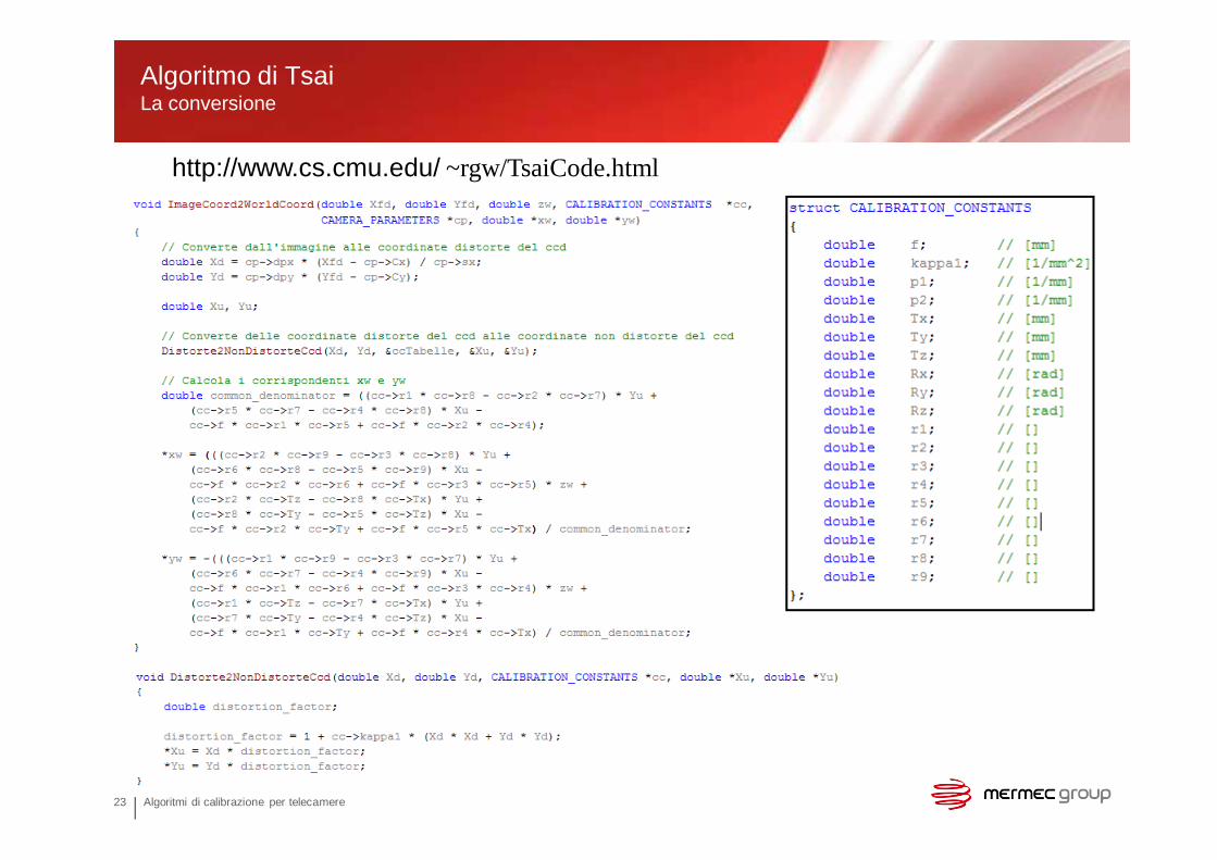
Algoritmo di TsaiLa conversione

http://www.cs.cmu.edu/ ~rgw/TsaiCode.html


Algoritmo di Zhang

Zhang esegue un aggiornamento delle tecniche di calibrazione di Tsai.

Zhang calcola la matrice H e da questa cerca di ricavare i parametri in maniera esplicita. H è una matrice omografica e pertanto possiede 8 gradi di libertà. Da questa matrice è possibile porre due vincoli basati sulla ortonormalità della matrice di rotazione forzando almeno 2 dei parametri della matrice dei parametri intrinseci.

Esprimendo l'ortonormalità tra i vettori colonna:

=

=

~~

2

~

1

~

3

~

2

~

1 trrAhhhH λ

0~

2

~

1 =hWhT ~

2

~

2

~

1

~

1 hWhhWh TT = 11)( −−= AAW T

Le incognite della matrice W possono essere risolte usando almeno 2 (o 3) piani diversi, ovvero matrici le cui colonne non siano linearmente dipendenti tra loro.Determinata la matrice con una decomposizione di Choleski si può determinare la matrice originale. Tuttavia Zhang fornisce le equazioni per ottenere i parametri direttamente da W decomponendola.


Cenni di triangolazione laserPrincipio 1

Si lega la posizione del target ad una posizione su un CCD basandosi sulle caratteristiche geometriche che dunque devono restare invariate. Quando queste variano si deve ricalibrare il sistema.


Cenni di triangolazione laserPrincipio 2

Si lega la posizione del target ad una posizione su un CCD basandosi sulle caratteristiche geometriche. Il laser fornisce il piano su cui si effettueranno le misure.

D1 = distanza tra sorgente laser P1 e telecamera P2 è costante e dettata da considerazioni meccaniche, come A1 angolo del fascio laser posto a 90°.L’inclinazione dell’asse delle telecamera A2 è anch’essocalcolato in funzione di considerazioni sulla misura.

In conclusione la distanza Da tra P1 e il punto damisurare Pa è:

Da = D1*tan(A2)


Cenni di triangolazione laserDiodi laser 1

Se su un atomo allo stato eccitato incide un fotone di frequenza opportuna, l'atomo si diseccita cedendo la sua energia sotto forma di fotone avente la stessa frequenza e la stessa fase di quello incidente.

Se si provoca la cosiddetta inversione della popolazione, cioè si fa in modo che gli atomi allo stato eccitato siano più numerosi di quelli allo stato fondamentale, si ha prevalenza dell'emissione stimolata sull'assorbimento. Il processo con cui si attua tale inversione prende il nome di pompaggio.

In un semiconduttore non si può considerare un atomo isolato, ma bisogna considerare tutto il cristallo nel suo insieme, con una certa distribuzione degli elettroni, che si dispongono in "bande" di energia. Operando una semplificazione si può dire che in un semiconduttore avremo una "banda di valenza" che risulterà "piena" di elettroni, ed una "banda di conduzione", ad energia più elevata, a distanza DE dalla banda di valenza, che conterrà pochi elettroni. Con diversi metodi è possibile ottenere all'interno del cristallo una vera e propria inversione di popolazione. Se non si inserisce il sistema in un risonatore (che può essere costituito dallo stesso cristallo di semiconduttore) si ottiene un LED altrimenti avremo un laser a semiconduttore. Esistono molti di questi laser, che emettono potenze medie di 10 mW in continua e raggiungono i 100 W in regime impulsato.


Cenni di triangolazione laserDiodi laser 2


Cenni di triangolazione laserClassi laser 1

.

CLASSE 1MLaser che emettono radiazione nell’ intervallo di lunghezze d’onda tra 302,5 nm e 4000 nm, sicuri nelle condizioni di funzionamento ragionevolmente prevedibili, ma che possono essere pericolosi se l’utilizzatore impiega ottiche (lenti di ingrandimento, etc.) all’ interno del fascio.CLASSE 2I laser in questa classe possono emettere radiazione pericolosa, ma la loro potenza è così bassa da risultare in qualche modo dannosa solo in caso di esposizione diretta e prolungata ovvero per un tempo superiore ai 0,25 secondi. Sono compresi in questa classe i laser ad emissione continua e nel visibile (400-700nm), con potenza ≤ 1mW.CLASSE 2MLaser che emettono radiazione visibile nell’ intervallo di lunghezze d’onda tra 400nm e 700nm, in cui la protezione dell’occhio è normalmente assicurata dalle reazioni di difesa compreso il riflesso palpebrale. Tuttavia l’osservazione dell’emissione può risultare pericolosa se, all’ interno del fascio, l’utilizzatore impiega ottiche (lenti di ingrandimento, etc.)


Cenni di triangolazione laserClassi laser 2

.

CLASSE 3R (CLASSE 3A)Sono compresi in questa classe i laser con emissione nel visibile e una potenza in uscita fino da 1mW a 5mW.Possono emettere radiazioni sia nel campo del visibile che in quello del non visibile e i loro fasci non sono pericolosi se osservati direttamente in maniera non continua, mentre lo possono diventare se si utilizzano strumenti che amplificano e concentrano il fascio ottico (quali microscopi, binocoli, ecc.).CLASSE 3BI laser di classe 3B hanno potenze medie comprese tra i 5mW e i 500 mW. I laser di classe 3B, sia perradiazione visibile che per quella non visibile, sono pericolosi per gli occhi se non protetti e possono essere pericolosi per la pelle; anche le riflessioni diffuse da questi sistemi possono essere pericolosi. Devono essere prese precauzioni per evitare lo stazionamento nella direzione del fascio o del fascio riflesso da una superficie.CLASSE 4Sono i laser più pericolosi in quanto, oltre ad avere una potenza tale da causare seri danni ad occhi e pelle anche se il fascio è diffuso, possono costituire un potenziale rischio di incendio, causare fuoruscita di materiale tossico e spesso il voltaggio e l’amperaggio di alimentazione sono pericolosamente elevati. Comprende tutti quei sistemi che superano i livelli imposti alla classe 3B.


Cenni di triangolazione laserSicurezza

Un fascio di luce laser sia diretto, che riflesso da superfici speculari può causare danni anche irreversibili alle strutture oculari e alla pelle; la natura di questi danni dipende dalla lunghezza d’onda della radiazione, mentre la gravità è legata alla densità di potenza E (per sorgenti in funzionamento continuo) o alla densità di energia H (per fasci in funzionamento impulsato) e al tempo in cui la struttura oculare è esposta al fascio laser.

Confronto tra il sole e un laser:

SOLE: Intensitàmassima luce solare a terra = 1 kW/m2 o 1 mW/mm2

Assumendo un diametro pupillare di 2 mm l’area è circa 3 mm2

Quindi la potenza raccolta dall’occhio è = 3 mWIl sole forma un’ immagine ≈ 100 µm di raggio sulla retina (area = 0.03 mm2)L’intensità sulla retina (Potenza/Area) = 3 mW/0.03 mm2 = 100 mW/mm2.

Tipico laser He Ne da 1 mW (o laser pointer):Potenza (P) = 1 mW (Classe 3R), raggio del fascio = 1 mmForma un’ immagine con raggio di 10 µm (area dello spot = 3 10-4 mm2)L’ intensità dell’He-Ne sulla retina è 1 mW/(3 10-4 mm2) = 3100 mW/mm2

31 volte l ’ intensit à del sole!!


Cenni di triangolazione laserTipi di Superificie

Il sistema a triangolazione laser fa uso della luce rifratta (non riflessa) da una superficie lambertiana.

Notare che parte della potenza del laser viene persa nel raggio riflesso. Il caso peggiore si ha nel caso di superfici lucide come gli specchi o superfici levigate.


Trasformata di Hough (HT)Cenni

Il problema del riconoscimento di oggetti in un immagine è spesso risolto usando algoritmi di pattern matching o simili minimizzando un indice di errore

Tali algoritmi sono spesso molto onerosi e soffrono in presenza di immagini rumorose o di sovrapposizione tra oggetti.

Permette di individuare forme descritte da equazioni analitiche (es. Rette). Essa trasforma un problema di ricerca di una curva in un più semplice problema di ricerca di massimi.

La HT gode delle seguenti proprietà:

⟩ Ogni punto dello spazio immagine corrisponde ad una superficie generalizzata nello spazio dei parametri;

⟩ N punti nello spazio immagine appartenenti alla stessa curva generano N superfici che si intersecano nello stesso punto dello spazio dei parametri;

Esistono poi le proprietà duali.


Trasformata di HoughCelle e voto

Si discretizza lo spazio dei parametri in celle di dimensione dipendente dalle precisioni richieste. Ad ogni cella corrisponde un’istanza quantizzata della curva. Definiamo dunque un accumulatore:

Un processo di voto viene poi implementato cosicchè ad ogni cella corrispondano tanti voti quante le superfici che la intersecano, ognuna delle quali generata da una curva dello spazio immagine.

Un processo di ricerca del massimo andrà poi a indentificare la curva con piùvoti, dunque molteintersezioni indicano la presenza della curva analiticacercata.

),( ρθAcc


Trasformata di Hough (HT) Esempio - rette 1

Per prima cosa si passa a coordinate polari perchè hanno variazione limitata:

La HT di una linea è un punto. Una stella di rette diviene un insieme di punticonnessi nello spazio di Hough:

θθρ sincos yx +=

Considerando un punto come centrodi una stella. L’intersezione dei punticorrispondenti (voto maggiore) nellospazio di Hough indica la retta i cui parametri sono identificati dalla cella.


Trasformata di Hough (HT) Esempio - rette 2

Andando a fare un esempio pratico si vede bene come trasformando tutti i punti dell’immagine una regione ristretta nello spazio di Hough (cella) è interessata da molte intersezioni cioè da molti voti.

Dalla cella cui è possibile ricavare le caratteristiche (pendenza ed intercetta) della retta che unisce i vari punti che l’hanno votata.

In altre parole vi sono N stelle di rette generate da N punti dell’immagine che hanno in comune la retta illustrata e questo si evince dal voto alto ad una cella.


Processo di calibrazioneAcquisizione del bersaglio in varie posizioni

Acquisizione del bersaglio forato in varie posizioni.

Il bersaglio è movimentato tramite un sistema motorizzato ad alta precisione. Si possono acquisire più telecamere alla volta:


Processo di calibrazione Identificazione primo set di parabole

Identificazione delle parabole:

1. eliminazione degli spigoli;

2. primo tentativo di fit con una retta;

3. Eliminazione punti troppoortoganli alla retta trovata;

4. Nuovo fit di una nuovaretta (miglioro la stima);

5. Eliminazione punti troppodistanti;

6. fit con una parabola;

Non si stima una retta perchè vi sono le distorsionidell’ottica


Processo di calibrazioneAssieme di tutte le acquisizioni del bersaglio

Si ricaricano in memoria tutte le tracce acquisite, una per ogni posizione del bersaglio. Si usano tutti i punti non appartenenti alle parabole già trovate per andare a fare una ricerca con Hough.


Processo di calibrazione Identificazione rette mediante trasformata di Hough

Tramite la trasformata di Hough si possono individure le rette ortogonali alle parabole già trovate imponendo un angolo di 90 gradi (con tolleranza!!!).

Se non si trovano tutte le rette si possono“suggerire” manualmente.

Per far ciò si eliminano ipunti già usati considerandola distanza tra punto e parabola e poi si da tutto in pasto alla HT.


Processo di calibrazione Trasformata di Hough


Processo di calibrazione Identificazione secondo set di parabole

Per prima cosa si ordinano le rette trovate con la HT in base all’intercetta.

Considerando solo i punti vicini alle rette trovate con la trasformata di Hough si identifica il secondo set di parabole.


Processo di calibrazione Identificazione degli incroci

A questo punto si hanno due set di parabole tra loro ortogonali. Si procede a determinare tutte le intersezioni che saranno i dati di ingresso all’algoritmo di calibrazione dato che si conoscono le distanze reali in X ed Y tra tali punti (1 cm).


Processo di calibrazione Algoritmo di Tsai - Verifica

Identificati i punti, si possono dare in ingresso all’algoritmo di calibrazione (qui Tsai) che identifica i parametri del modello.

A questo si possono trasformare i punti di incrocio dei due set di parabole usando la calibrazione appena fatta e confrontare il risultato con reticolo dato in pasto per la calibrazione.

La focale è un parametro importante perchèda subito l’idea della bonta della calibrazione.

L’errore massimo dipende dal grado diadeguatezza del modello e spesso riguardaporzioni di campo che poi non verrannoutilizzate.

La media dell’errore e la standard deviation sonogli indici della bontà della calibrazione.


L’obiettivo


Il diaframma

Come si nota dalla figura i raggi che sono raccolti dal bordo della lente subiscono la maggior deflessione. Questo fa si che in tali zone il modello usato sia meno efficace.

Per attenuare tale fenomeno è conveniente chiudereun pò il diaframma tenendo presente anche le seguenticaratteristiche:

• Chiudendo il diaframma la profondità di campo aumenta (cosa non molto utile se si inclina ilCCD);• Aprendo il diaframma la luminosità aumenta;

Bisogna dunque bilanciare i due fenomeni.


10 Regole d’oro

1. Raccogliere tutte le informazioni di progetto, in particolare:– i disegni 3D del montaggio della dima di calibrazione;– gli schemi recanti il campo di visione con le quote orizzontali, verticali

(e oblique se possibile) rispetto alla base del calibratore e rispetto ad un punto ben identificabile della cassa;

2. Raccogliere i dati sulla focale degli obiettivi;3. Verificare che il sistema non si debba più manopolare; 4. Test del sistema di movimentazione del bersaglio;5. Verificare la messa a fuoco del laser e della telecamera in tutto il campo

di visione e dell'allineamento dei laser sul bersaglio posto a metà del campo di visione;

6. Regolare i parametri in tutto il campo di visione per eliminare i disturbi e vedere bene il bersaglio;

7. Effettuare la calibrazione in modo che la cassa od il bersaglio non vibrino o peggio si spostino;

8. Verifica risultati di calibrazione (focale, errore medio e massimo); 9. Convertire in millimetri e verificare che si misurino bene le distanze in X

ed Y movimentando il calibro; 10.Verificare che un bersaglio rettilineo posto obliquo non venga convertito

con una spezzata.


Esempi applicazioni Tecnogamma Mermec GroupTipi di veicolo


Esempi applicazioni Tecnogamma Mermec GroupInstallazione sezione per Track Geometry

Track Gauge

Rolling Plane

Calculated from

Real Rail Profiles

Laser Beam

Gauge Point 14 mm under Rolling Plane


Esempi applicazioni Tecnogamma Mermec GroupTrack Geometry e Rail Profile

Usura

ScartamentoLivelli Longitudinali

via Oberdan, 7070043 Monopoli (BA) Italyph. +39 080 8876570fax +39 080 8874028www.mermec.com

Technical Center220 Outlet Pointe Blvd.Columbia, SC 29210, USAph. +1 803 213 1200fax +1 803 798 1909www.imagemap.com

Technopôle de Château-GombertLes Baronnies - Bat. Arue Paul Langevin13013 Marseille (France)ph. +33 (0)4 91100190fax +33 (0)4 91086040www.inno-tech.fr

www.mermecgroup.com

vicolo Ongarie, 1331050 Morgano (TV), Italyph. +39 0422 8391fax +39 0422 839200www.tecnogamma.eu

Tsai’s camera calibration method revisited

Berthold K.P. Horn

Copright © 2000

Introduction

Basic camera calibration is the recovery of the principle distance f and the princi-ple point (x0, y0)

T in the image plane — or, equivalently, recovery of the positionof the center of projection (x0, y0, f )T in the image coordinate system. This isreferred to as interior orientation in photogrammetry.

A calibration target can be imaged to provide correspondences betweenpoints in the image and points in space. It is, however, generally impractical toposition the calibration target accurately with respect to the camera coordinatesystem using only mechanical means. As a result, the relationship between thetarget coordinate system and the camera coordinate system typically also needs tobe recovered from the correspondences. This is referred to as exterior orientationin photogrammetry.

Since cameras often have appreciable geometric distortions, camera calibra-tion is often taken to include the recovery of power series coefficients of thesedistortions. Furthermore, an unknown scale factor in image sampling may alsoneed to be recovered, because scan lines are typically resampled in the framegrabber, and so picture cells do not correspond discrete sensing elements.

Note that in camera calibration we are trying to recover the transforma-tions, based on measurements of coordinates, where one more often uses knowntransformation to map coordinates from one coordinate system to another.

Tsai’s method for camera calibration recovers the interior orientation, theexterior orientation, the power series coefficients for distortion, and an imagescale factor that best fit the measured image coordinates corresponding to knowntarget point coordinates. This is done in stages, starting off with closed form least-squares estimates of some parameters and ending with an iterative non-linearoptimization of all parameters simultaneously using these estimates as startingvalues. Importantly, it is error in the image plane that is minimized.

Details of the method are different for planar targets than for targets occu-pying some volume in space. Accurate planar targets are easier to make, but leadto some limitations in camera calibration, as pointed out below.

2

Interior Orientation — Camera to Image

Interior Orientation is the relationship between camera-centric coordinates andimage coordinates. The camera coordinate system has its origin at the center ofprojection, its z axis along the optical axis, and its x and y axes parallel to the xand y axes of the image.

Camera coordinates and image coordinates are related by the perspectiveprojection equations:

xI − x0

f= xC

zCand

yI − y0

f= yC

zCwhere f is the principle distance (distance from the center of projection to theimage plane), and (x0, y0) is the principle point (foot of the perpendicular fromthe center of projection to the image plane). That is, the center of projection isat (x0, y0, f )T , as measured in the image coordinate system.

Interior orientation has three degrees of freedom. The problem of interiororientation is the recovery of x0, y0, and f . This is the basic task of cameracalibration. However, as indicated above, in practice we also need to recover theposition and attitude of the calibration target in the camera coordinate system.

Exterior Orientation — Scene to Camera

Exterior Orientation is the relationship between a scene-centered coordinate sys-tem and a camera-centered coordinate system. The transformation from sceneto camera consists of a rotation and a translation. This transformation has sixdegrees of freedom, three for rotation and three for translation.

The scene coordinate system can be any system convenient for the partic-ular design of the target. In the case of a planar target, the z axis is chosenperpendicular to the plane, and z = 0 in the target plane.

If rS are the coordinates of a point measured in the scene coordinate systemand rC coordinates measured in the camera coordinate system, then

rC = R(rS )+ t

where t is the translation and R(. . .) the rotation.If we chose for the moment to use an orthonormal matrix to represent rota-

tion, then we can write this in component form:⎛⎝xC

yCzC

⎞⎠ =

⎛⎝r11 r12 r13r21 r22 r23r31 r32 r33

⎞⎠⎛⎝xS

ySzS

⎞⎠+

⎛⎝txtytz

⎞⎠

where rC = (xC , yC , zC )T , rS = (xS , yS , zS )

T , and t = (tx , ty , tz)T .

The unknowns to be recovered in the problem of exterior orientation are thetranslation vector t and the rotation R(. . .).

3

The Unknown Horizontal Scale Factor

A complicating factor in the calibration of many modern electronic cameras isthat the discrete nature of image sampling is not preserved in the signal.

In typical CCD or CMOS cameras, the initially discrete (staircase) sensorsignal in analog form is low pass filtered to produce a smooth video output signalin standard form that hides the transitions between cells of the sensor. Thiswaveform is then digitized in the frame grabber. The sampling in the horizontaldirection in the frame grabber is typically not equal to the spacing of sensorcells, and is not known accurately. The horizontal spacing between pixels in thesampled image do not in general correspond to the horizontal spacing betweencells in the image sensor.

This is in contrast with the vertical direction where sampling is controlled bythe spacing of rows of sensor cells. Some digital cameras avoid the intermediateanalog waveform and the low pass filtering, but many cameras — particularlycheaper ones intended for the consumer market — do not.

In this case the ratio of picture cell size in the horizontal and in the verticaldirection is not known a priori from the dimensions of the sensor cells and needsto be determined. This can be done separately using frequency domain methodsexploiting limitations of the approximate low pass filter and resulting aliasingeffects.

Alternatively, the extra scaling parameter can be recovered as part of thecamera calibration process. In this case we use a modified equation for xI :

xI − x0

f= s

xC

zC

where s is the unknown ratio of the pixel spacing in the x- and y-directions

It is not possible to recover this extra parameter when using planar targets,as discussed below, and so it has to be estimated separately in that case.

Combining Interior and Exterior Orientation

If we combine the equations for interior and exterior orientation we obtain:

xI − x0

f= s

r11xS + r12yS + r13zS + tx

r31xS + r32yS + r33zS + tzyI − y0

f= r21xS + r22yS + r23zS + ty

r31xS + r32yS + r33zS + tz

4

Distortion

Projection in an ideal imaging system is governed by the pin-hole model. Realoptical systems suffer from a number of inevitable geometric distortions. Inoptical systems made of spherical surfaces, with centers along the optical axis,a geometric distortion occurs in the radial direction. A point is imaged at adistance from the principle point that is larger (pin-cushion distortion) or smaller(barrel distortion) than predicted by the perspective projection equations; thedisplacement increasing with distance from the center. It is small for directionsthat are near parallel to the optical axis, growing as some power series of theangle. The distortion tends to be more noticable with wide-angle lenses thanwith telephoto lenses.

The displacement due to radial distortion can be modelled using the equa-tions:

δx = x(κ1r2 + κ2r

4 + . . .)

δy = y(κ1r2 + κ2r

4 + . . .)

where x and y are measured from the center of distortion, which is typicallyassumed to be at the principle point. Only even powers of the distance r fromthe principle point occur, and typically only the first, or perhaps the first and thesecond term in the power series are retained.

Electro-optical systems typically have larger distortions than optical systemsmade of glass. They also suffer from tangential distortion, which is at right angleto the vector from the center of the image. Like radial distortion, tangentialdistortion grows with distance from the center of distortion.

δx = −y(ε1r2 + ε2r

4 + . . .)

δy = +x(ε1r2 + ε2r

4 + . . .)

In calibration, one attempts to recover the coefficients (κ1, . . . , ε1, . . .) of thesepower series. It is also possible to recover distortion parameters separately using,for example, the method of plumb lines.

Note that one can express the actual (distorted) image coordinates as apower series using predicted (undistorted) image coordinates as variables, or onecan express predicted image coordinates as a power series in the actual imagecoordinates (that is, the r in the above power series can be either based on actualimage coordinates or predicted image coordinates). The power series in the twocases are related by inversion.

If the power series to adjust distorted coordinates to undistorted coordinatesis used, then it is more convenient to do the final optimization in undistorted imagecoordinates rather than distorted (actual) image coordinates.

5

If instead the power series to adjust undistorted coordinates to distortedcoordinates is used, then it is more convenient to do the final optimization in dis-torted (actual) image coordinates rather than the undistorted image coordinates.

Overall strategy

In calibration, a target of known geometry is imaged. Correspondences betweentarget points and their images are obtained. These form the basic data on whichthe calibration is based.

Tsai’s method first tries to obtain estimates of as many parameters as possibleusing linear least-squares fitting methods. This is convenient and fast since suchproblems can be solved using the pseudo-inverse matrix.

In this initial step, constraints between parameters (such as the orthonormal-ity of a rotation matrix) are not enforced, and what is minimized is not the errorin the image plane, but a quantity that simplifies the analysis and leads to linearequations. This does not affect the final result, however, since these estimatedparameter values are used only as starting values for the final optimization.

In a subsequent step, the rest of the parameters are obtained using a non-linear optimization method that finds the best fit between the observed imagepoints and those predicted from the target model. Parameters estimated in thefirst step are refined in the process.

Details of the calibration method are different when the target is planarthen when it is not. Accurate planar targets are easier to make and maintainthan three-dimensional targets, but limit calibration in ways that will becomeapparent. We start by analysing the case of the non-coplanar target.

Estimating the rotation, and part of the translation

Initally we assume that we have a reasonable estimate of the position of theprinciple point (x0, y0). This point is usually near the middle of the CCD orCMOS sensor. We refer coordinates to this point using

x′I = xI − x0 and y′

I = yI − y0

so thatx′I

f= s

xC

zCand

y′I

f= yC

zCNext, we consider only the direction of the point in the image as measured fromthe principle point. This yields a result that is independent of the unknownprinciple distance f . It is also independent of radial distortion.

x′I

y′I

= sxC

yC

6

Using the expansion in terms of components of the rotation matrix R we obtain:

x′I

y′I

= sr11xS + r12yS + r13zS + tx

r21xS + r22yS + r23zS + ty

which becomes, after cross multiplying:

s(r11xS + r12yS + r13zS + tx)y′I − (r21xS + r22yS + r23zS + ty)x

′I = 0

or(xSy

′I )sr11 + (ySy

′I )sr12 + (zSy

′I )sr13 + y′

I stx

−(xSx′I )r21 − (ySx

′I )r22 − (zSx

′I )r23 − x′

I ty = 0

which we can view as a linear homogeneous equation in the eight unknowns

sr11, sr12, sr13, r21, r22, r23, stx , and ty

The coefficients in the equation are products of components of correspondingscene and image coordinates.

We obtain one such equation for every correspondence between a calibrationtarget point (xS i , yS i , zS i)

T and an image point (xI i , yI i)T .

Note that there is an unknown scale factor here because these equations arehomogeneous. That is, if we have a solution for the eight unknowns, then anymultiple of that solution is also a solution. In order to obtain a solution, we canconvert the homogeneous equation into inhomogeneous equation by arbitrarilysetting one unknown — ty say — to one.

We then have seven unknowns for which we can solve if we have seven corre-spondences between target coordinates and image coordinates. If we have morethan seven correspondences, we can minimize the sum of squares of errors usingthe pseudo-inverse method.

When we obtain the solution, we do have to remember that the eight un-knowns (the seven we solved for plus the one we set to one) can be scaled by anarbitrary factor. Suppose that the best fit solution of the set of equations is

sr ′11, sr ′12, sr ′13, st ′x , r ′21, r ′22, r ′23, and t ′y = 1

We can estimate the correct scale factor by noting that the rows of the rotationmatrix are supposed to be normal, that is

r211 + r212 + r213 = 1 and r221 + r222 + r223 = 1

We need to find the scale factor c to be applied to the solution to satisfy theseequalities. It is easy to see that

c = 1/√r ′221 + r ′222 + r ′223

andc/s = 1/

√(sr ′11)2 + (sr ′12)2 + (sr ′13)2

These equations allow us to recover the factor c as well as the ratio s of thehorizontal pixel spacing to the vertical pixel spacing.

7

Note that we did not enforce the orthogonality of the first two rows ofthe rotation matrix. We can improve matters by adjusting them to make themorthogonal.

Forcing orthonormality of the first two rows

Given the vectors a and b, we can find two orthogonal vectors a′ and b′ that areas near as possible to a and b as follows:

a′ = a + kb and b′ = b + ka

a′ · b′ = a · b + k(a · a + b · b)+ k2a · b = 0

The solution of this quadratic for k tends to be numerically ill behaved since thefirst and last coefficients (a · b) are small when the vectors are already close tobeing orthogonal. The following approximate solution can be used then

k ≈ −(1/2)a · b

(since k is expected to be small and a · a and b · b near one).We have to renormalize the first two rows of the rotation matrix after ad-

justing them to make them orthogonal.Finally we can obtain the third row of the rotation matrix simply by tak-

ing the cross-product of the first two rows. The resulting 3 × 3 matrix will beorthonormal if we performed the above orthonormalization of the first two rows.

Note that there may be problems with this method of solution if the un-known (ty) that we decided to set equal to one in order to solve the homogeneousequations happens to be near zero. In this case a solution may be obtained bysetting another unknown (tx perhaps) equal to one. An alternative is to translatethe experimental data by some offset in y.

Also note that we did not minimize the error in the image, but some otherquantitity that led to convenient, linear equations. The resulting rotation matrixand translation components are not especially accurate as a result. This is ac-ceptable only because we use the recovered values merely as estimates in the fullnon-linear optimization described below.

Coplanar Target

The above method cannot be used as is when the target is planar. It turns outthat we cannot recover the scale factor s in this case, so we assume that imagecoordinates have already been adjusted to account for any differences in scalingin the x and y directions.

With a planar target we can always arrange the coordinate system such thatzS = 0 for points on the target. This means the products with r13, r23, and r33

8

drop out of the equations for the image coordinates and we obtain:

x′I

y′I

= r11xS + r12yS + tx

r21xS + r22yS + ty

which becomes, after cross multiplying:

(r11xS + r12yS + tx)y′I − (r21xS + r22yS + ty)x

′I = 0

or

(xSy′I )r11 + (ySy

′I )r12 + y′

I tx − (xSx′I )r21 − (ySx

′I )r22 − x′

I ty = 0

a linear homogeneous equation in the six unknowns

r11, r12, r21, r22, tx , and ty

The coefficients in this equation are products of components of correspondingscene and image coordinates.

We obtain one such equation for every correspondence between a calibrationtarget point (xS i , yS i , zS i)

T and an image point (xI i , yI i)T .

As in the non-coplanar case, there is an unknown scale factor because theseequations are homogeneous. If we have a solution for the six unknowns, thenany multiple of that solution is also a solution. We can convert the homogeneousequations into inhomogeneous equations by arbitrarily setting one unknown —ty say — to one.

We then have five unknowns for which we can solve if we have five corre-spondences between target coordinates and image coordinates. If we have morethan five correspondences, we can minimize the sum of squares of errors usingthe pseudo-inverse.

We do have to remember though that the six unknowns (the five we solvedfor plus the one we set equal to one) can be scaled by an arbitrary factor.

Suppose that the best fit solution of the set of equations is

r ′11, r ′12, r ′21, r ′22, t ′x , and t ′y = 1

We now are faced with the task of estimating the full 3× 3 rotation matrix basedonly on its top left 2× 2 sub-matrix.

Recovering the full rotation matrix for planar target

We can estimate the correct scale factor by noting that the rotation matrix issupposed to be orthonormal and hence

r211 + r212 + r213 = 1

r221 + r222 + r223 = 1

r11r21 + r12r22 + r13r23 = 0

9

so we haver ′211 + r ′212 + r ′213 = k2

r ′221 + r ′222 + r ′223 = k2

r ′11r ′21 + r ′12r ′22 + r ′13r ′23 = 0

From the first two equations we have

(r ′211 + r ′212)(r ′221 + r ′222) = (k2 − r ′213)(k2 − r ′223)From the third equation we get

(r ′11r ′21 + r ′12r ′22)2 = (r ′13r ′23)2

Subtracting we obtain

(r ′11r ′22 − r ′12r ′21)2 = k4 − k2(r ′213 + r ′223)Since

(r ′213 + r ′223) = 2k2 − (r ′211 + r ′212 + r ′221 + r ′222)we end up with

k4 − k2(r ′211 + r ′212 + r ′221 + r ′222)+ (r ′11r ′22 − r ′12r ′21)2 = 0

a quadratic in k2. This then allows us to calculate the missing coefficients r ′13and r ′23 in the first two rows of the rotation matrix using

r ′213 = k2 − (r ′211 + r ′212)

r ′223 = k2 − (r ′221 + r ′222)Only the more positive of the two roots for k2 makes the right hand sides of theseequations positive, so we only need to consider that root.

k2 = 1

2

((r ′211 + r ′212 + r ′221 + r ′222)

+√(

(r ′11 − r ′22)2 + (r ′12 + r ′21)2)((r ′11 + r ′22)2 + (r ′12 − r ′21)2

))

We normalize the first two rows of the rotation matrix by dividing by k. Finally,we make up the third row by taking the cross-product of the first two rows.

There are, however, sign ambiguities in the calculation of r ′13 and r ′23. Wecan get the sign of the product r ′13r ′23 using the fact that

r13r23 = −(r11r21 + r12r22)

so there is only a two-way ambiguity — but we do need to pick the proper signto get the proper rotation matrix.

One way to pick the correct signs for r13 and r23 is to use the resulting trans-formation to project the target points back into the image. If the signs are correct,the predicted image positions will be close to the observed image positions. Ifthe signs of these two components of the rotation matrix are picked incorrectly,then the first two components of the third row of the estimated rotation matrixwill be wrong also, since that row is the cross-product of the first two. As a result

10

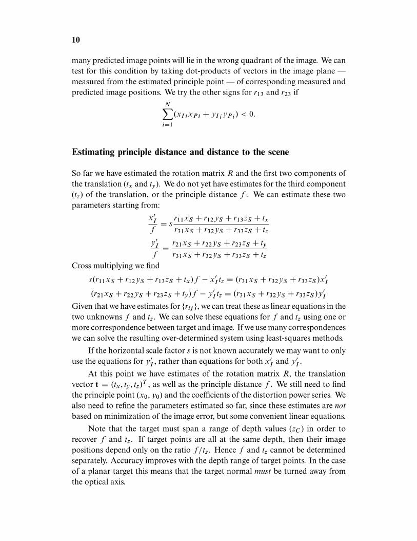
many predicted image points will lie in the wrong quadrant of the image. We cantest for this condition by taking dot-products of vectors in the image plane —measured from the estimated principle point — of corresponding measured andpredicted image positions. We try the other signs for r13 and r23 if

N∑i=1

(xI ixP i + yI iyP i) < 0.

Estimating principle distance and distance to the scene

So far we have estimated the rotation matrix R and the first two components ofthe translation (tx and ty). We do not yet have estimates for the third component(tz) of the translation, or the principle distance f . We can estimate these twoparameters starting from:

x′I

f= s

r11xS + r12yS + r13zS + tx


y′I

f= r21xS + r22yS + r23zS + ty


Cross multiplying we find

s(r11xS + r12yS + r13zS + tx)f − x′I tz = (r31xS + r32yS + r33zS )x

′I

(r21xS + r22yS + r23zS + ty)f − y′I tz = (r31xS + r32yS + r33zS )y

′I

Given that we have estimates for {rij }, we can treat these as linear equations in thetwo unknowns f and tz . We can solve these equations for f and tz using one ormore correspondence between target and image. If we use many correspondenceswe can solve the resulting over-determined system using least-squares methods.

If the horizontal scale factor s is not known accurately we may want to onlyuse the equations for y′

I , rather than equations for both x′I and y′

I .

At this point we have estimates of the rotation matrix R, the translationvector t = (tx , ty , tz)

T , as well as the principle distance f . We still need to findthe principle point (x0, y0) and the coefficients of the distortion power series. Wealso need to refine the parameters estimated so far, since these estimates are notbased on minimization of the image error, but some convenient linear equations.

Note that the target must span a range of depth values (zC ) in order torecover f and tz . If target points are all at the same depth, then their imagepositions depend only on the ratio f/tz . Hence f and tz cannot be determinedseparately. Accuracy improves with the depth range of target points. In the caseof a planar target this means that the target normal must be turned away fromthe optical axis.

11

Non-linear optimization

At this point we minimize the image errors, that is, the difference between theobserved image positions (xI , yI )

T and the positions (xP , yP )T predicted based

on the known target coordinates (xS , yS , zS )T . The parameters of interior ori-

entation, exterior orientation and distortion are adjusted to minimizeN∑i=1

(xI i − xP i)2 +

N∑i=1

(yI i − yP i)2

This is best done using iterative numerical optimization such as a modifiedLevenberg-Marquardt method.

Non-linear optimization methods work best when they have full access tothe components of the error. In the case here, it is best to treat (xI i − xP i) and(yI i−yP i) as separate error components rather than, for example, lumping theminto a combined error term of the form√

(xI i − xP i)2 + (yI i − yP i)2

Representation of rotation

To use non-linear optimization methods we need a non-redundant parameter-ization for rotation. Orthonormal matrices are redundant since they use ninenumbers to represent just three degrees of freedom. Maintaining the six con-straints of orthonormality in the minimization is very difficult.

Tsai’s original method used Euler angles to represent rotations. An alterna-tive is the Gibb’s vector

ω tan(θ/2)

The direction of the Gibb’s vector is the axis about which the rotation takes place,ω, while its magnitude is the tangent of half the angle of rotation, θ . Like all non-redundant representations for rotation, the Gibb’s vector has a singularity. Itoccurs when the rotation is through π radians.

An alternative is to use a redundant representation that has no singularities— and enforce the required non-linear constraint. The axis-and-angle repre-sentation of rotation can be related to the unit quaternion notation. The unitquaternion for the rotation is

q = (cos(θ/2), ω sin(θ/2)

)

The needed constraint that this be a unit vector is easily incorporated in thenon-linear optimization by adding an error term of the form

(q · q − 1)2

12

Sensitivity of solution

Error in the calibration parameters is directly proportional to error in imagemeasurements. The proportionality factor depends on the imaging geometry,and on the design of the target. Some parameters of the calibration are moresensitive to error than others, and some behave worse when the field of view isnarrow or the depth range of the target limited.

It is difficult to investigate the sensitivities to noise analytically because of thenon-linearity of the imaging model. However, the sensitivity issue can be studiedeasily using Monte Carlo simulation. Add random noise to the calibration imagedata and recompute the calibration parameters. Repeat and collect mean andcovariance statistics.

References and Acknowledgements

Horn, B.K.P. (1986) Robot Vision, MIT Press, Cambridge, Massachusetts andMcGraw-Hill, New York.

Horn, B.K.P. (1987) “Closed Form Solution of Absolute Orientation using UnitQuaternions,’’ Journal of the Optical Society A, Vol. 4, No. 4, pp. 629–642,April.

Horn, B.K.P., H. M. Hilden & S. Negahdaripour, (1988) “Closed Form Solu-tion of Absolute Orientation using Orthonormal Matrices,’’ Journal of theOptical Society A, Vol. 5, No. 7, pp. 1127–1135, July.

Horn, B.K.P. (1990) “Relative Orientation,’’ International Journal of ComputerVision, Vol. 4, No. 1, pp. 59–78, January.

Horn, B.K.P. (1991) “Relative Orientation Revisited,’’ Journal of the Optical So-ciety of America, A, Vol. 8, pp. 1630–1638, October.

Tsai, Roger Y. (1986) “An Efficient and Accurate Camera Calibration Techniquefor 3D Machine Vision,’’ Proceedings of IEEE Conference on Computer Vi-sion and Pattern Recognition, Miami Beach, FL, 1986, pp. 364–374.

Tsai, Roger Y. (1987) “A Versatile Camera Calibration Technique for High-Accuracy 3D Machine Vision Metrology Using Off-the-Shelf TV Camerasand Lenses,’’ IEEE Journal of Robotics and Automation, Vol. RA–3, No. 4,August 1987, pp. 323–344.

An implementation of Tsai’s method dating to 1995 by Reg Willson of 3M inSt. Paul, MN may be found on the web. Willson further acknowledges PiotrJasiobedzki, Jim Vaughan, Ron Steriti, Torfi Thorhallsson, Frederic Devernay,Volker Rodehorst, and Jon Owen.

13

The public domain MINPACK “lmdif’’ package can be used for the non-linear optimization. This uses a modified Levenberg-Marquardt algorithm witha Jacobian calculated by a forward-difference approximation.

A Flexible New Technique for CameraCalibration

Zhengyou Zhang

December 2, 1998(updated on December 14, 1998)

(updated on March 25, 1999)(updated on Aug. 10, 2002; a typo in Appendix B)

(last updated on Aug. 13, 2008; a typo in Section 3.3)

Technical ReportMSR-TR-98-71

Microsoft ResearchMicrosoft Corporation

One Microsoft WayRedmond, WA 98052

[email protected]://research.microsoft.com/˜zhang

A Flexible New Technique for Camera Calibration

Zhengyou ZhangMicrosoft Research, One Microsoft Way, Redmond, WA 98052-6399, USA

[email protected] http://research.microsoft.com/˜zhang

Contents

1 Motivations 2

2 Basic Equations 32.1 Notation . . . . . . . . . . . . . . . . . . . . . . . . . . . . . . . . . . . . . . . . . 32.2 Homography between the model plane and its image . . . . . . . . . . . . . . . . . 42.3 Constraints on the intrinsic parameters . . . . . . . . . . . . . . . . . . . . . . . . . 42.4 Geometric Interpretation† . . . . . . . . . . . . . . . . . . . . . . . . . . . . . . . . 4

3 Solving Camera Calibration 53.1 Closed-form solution . . . . . . . . . . . . . . . . . . . . . . . . . . . . . . . . . . 53.2 Maximum likelihood estimation . . . . . . . . . . . . . . . . . . . . . . . . . . . . 63.3 Dealing with radial distortion . . . . . . . . . . . . . . . . . . . . . . . . . . . . . . 73.4 Summary . . . . . . . . . . . . . . . . . . . . . . . . . . . . . . . . . . . . . . . . 8

4 Degenerate Configurations 8

5 Experimental Results 95.1 Computer Simulations . . . . . . . . . . . . . . . . . . . . . . . . . . . . . . . . . 95.2 Real Data . . . . . . . . . . . . . . . . . . . . . . . . . . . . . . . . . . . . . . . . 105.3 Sensitivity with Respect to Model Imprecision‡ . . . . . . . . . . . . . . . . . . . . 14

5.3.1 Random noise in the model points . . . . . . . . . . . . . . . . . . . . . . . 145.3.2 Systematic non-planarity of the model pattern . . . . . . . . . . . . . . . . . 15

6 Conclusion 17

A Estimation of the Homography Between the Model Plane and its Image 17

B Extraction of the Intrinsic Parameters from Matrix B 18

C Approximating a 3× 3 matrix by a Rotation Matrix 18

D Camera Calibration Under Known Pure Translation§ 19

†added on December 14, 1998‡added on December 28, 1998; added results on systematic non-planarity on March 25, 1998§added on December 14, 1998, corrected (based on the comments from Andrew Zisserman) on January 7, 1999

1

A Flexible New Technique for Camera Calibration

Abstract

We propose a flexible new technique to easily calibrate a camera. It is well suited for usewithout specialized knowledge of 3D geometry or computer vision. The technique only requiresthe camera to observe a planar pattern shown at a few (at least two) different orientations. Eitherthe camera or the planar pattern can be freely moved. The motion need not be known. Radial lensdistortion is modeled. The proposed procedure consists of a closed-form solution, followed by anonlinear refinement based on the maximum likelihood criterion. Both computer simulation andreal data have been used to test the proposed technique, and very good results have been obtained.Compared with classical techniques which use expensive equipment such as two or three orthog-onal planes, the proposed technique is easy to use and flexible. It advances 3D computer visionone step from laboratory environments to real world use.

Index Terms— Camera calibration, calibration from planes, 2D pattern, absolute conic, projectivemapping, lens distortion, closed-form solution, maximum likelihood estimation, flexible setup.

1 Motivations

Camera calibration is a necessary step in 3D computer vision in order to extract metric informationfrom 2D images. Much work has been done, starting in the photogrammetry community (see [2,4] to cite a few), and more recently in computer vision ([9, 8, 23, 7, 26, 24, 17, 6] to cite a few).We can classify those techniques roughly into two categories: photogrammetric calibration and self-calibration.

Photogrammetric calibration. Camera calibration is performed by observing a calibration objectwhose geometry in 3-D space is known with very good precision. Calibration can be done veryefficiently [5]. The calibration object usually consists of two or three planes orthogonal to eachother. Sometimes, a plane undergoing a precisely known translation is also used [23]. Theseapproaches require an expensive calibration apparatus, and an elaborate setup.

Self-calibration. Techniques in this category do not use any calibration object. Just by moving acamera in a static scene, the rigidity of the scene provides in general two constraints [17, 15]on the cameras’ internal parameters from one camera displacement by using image informa-tion alone. Therefore, if images are taken by the same camera with fixed internal parameters,correspondences between three images are sufficient to recover both the internal and externalparameters which allow us to reconstruct 3-D structure up to a similarity [16, 13]. While this ap-proach is very flexible, it is not yet mature [1]. Because there are many parameters to estimate,we cannot always obtain reliable results.

Other techniques exist: vanishing points for orthogonal directions [3, 14], and calibration from purerotation [11, 21].

Our current research is focused on a desktop vision system (DVS) since the potential for usingDVSs is large. Cameras are becoming cheap and ubiquitous. A DVS aims at the general public,who are not experts in computer vision. A typical computer user will perform vision tasks only fromtime to time, so will not be willing to invest money for expensive equipment. Therefore, flexibility,robustness and low cost are important. The camera calibration technique described in this paper wasdeveloped with these considerations in mind.

2

The proposed technique only requires the camera to observe a planar pattern shown at a few (atleast two) different orientations. The pattern can be printed on a laser printer and attached to a “rea-sonable” planar surface (e.g., a hard book cover). Either the camera or the planar pattern can be movedby hand. The motion need not be known. The proposed approach lies between the photogrammet-ric calibration and self-calibration, because we use 2D metric information rather than 3D or purelyimplicit one. Both computer simulation and real data have been used to test the proposed technique,and very good results have been obtained. Compared with classical techniques, the proposed tech-nique is considerably more flexible. Compared with self-calibration, it gains considerable degree ofrobustness. We believe the new technique advances 3D computer vision one step from laboratoryenvironments to the real world.

Note that Bill Triggs [22] recently developed a self-calibration technique from at least 5 views ofa planar scene. His technique is more flexible than ours, but has difficulty to initialize. Liebowitz andZisserman [14] described a technique of metric rectification for perspective images of planes usingmetric information such as a known angle, two equal though unknown angles, and a known lengthratio. They also mentioned that calibration of the internal camera parameters is possible provided atleast three such rectified planes, although no experimental results were shown.

The paper is organized as follows. Section 2 describes the basic constraints from observing asingle plane. Section 3 describes the calibration procedure. We start with a closed-form solution,followed by nonlinear optimization. Radial lens distortion is also modeled. Section 4 studies con-figurations in which the proposed calibration technique fails. It is very easy to avoid such situationsin practice. Section 5 provides the experimental results. Both computer simulation and real data areused to validate the proposed technique. In the Appendix, we provides a number of details, includingthe techniques for estimating the homography between the model plane and its image.

2 Basic Equations

We examine the constraints on the camera’s intrinsic parameters provided by observing a single plane.We start with the notation used in this paper.

2.1 Notation

A 2D point is denoted by m = [u, v]T . A 3D point is denoted by M = [X,Y, Z]T . We use x to denotethe augmented vector by adding 1 as the last element: m = [u, v, 1]T and M = [X, Y, Z, 1]T . A camerais modeled by the usual pinhole: the relationship between a 3D point M and its image projection m isgiven by

sm = A[R t

]M , (1)

where s is an arbitrary scale factor, (R, t), called the extrinsic parameters, is the rotation and trans-lation which relates the world coordinate system to the camera coordinate system, and A, called thecamera intrinsic matrix, is given by

A =

α γ u0

0 β v0

0 0 1

with (u0, v0) the coordinates of the principal point, α and β the scale factors in image u and v axes,and γ the parameter describing the skewness of the two image axes.

We use the abbreviation A−T for (A−1)T or (AT )−1.

3

2.2 Homography between the model plane and its image

Without loss of generality, we assume the model plane is on Z = 0 of the world coordinate system.Let’s denote the ith column of the rotation matrix R by ri. From (1), we have

s

uv1

= A

[r1 r2 r3 t

]

XY01

= A[r1 r2 t

]

XY1

.

By abuse of notation, we still use M to denote a point on the model plane, but M = [X, Y ]T since Z isalways equal to 0. In turn, M = [X, Y, 1]T . Therefore, a model point M and its image m is related by ahomography H:

sm = HM with H = A[r1 r2 t

]. (2)

As is clear, the 3× 3 matrix H is defined up to a scale factor.

2.3 Constraints on the intrinsic parameters

Given an image of the model plane, an homography can be estimated (see Appendix A). Let’s denoteit by H =

[h1 h2 h3

]. From (2), we have

[h1 h2 h3

]= λA

[r1 r2 t

],

where λ is an arbitrary scalar. Using the knowledge that r1 and r2 are orthonormal, we have

hT1 A−TA−1h2 = 0 (3)

hT1 A−TA−1h1 = hT

2 A−TA−1h2 . (4)

These are the two basic constraints on the intrinsic parameters, given one homography. Because ahomography has 8 degrees of freedom and there are 6 extrinsic parameters (3 for rotation and 3 fortranslation), we can only obtain 2 constraints on the intrinsic parameters. Note that A−TA−1 actuallydescribes the image of the absolute conic [16]. In the next subsection, we will give an geometricinterpretation.

2.4 Geometric Interpretation

We are now relating (3) and (4) to the absolute conic.It is not difficult to verify that the model plane, under our convention, is described in the camera

coordinate system by the following equation:[

r3

rT3 t

]T [xyzw

]= 0 ,

where w = 0 for points at infinity and w = 1 othewise. This plane intersects the plane at infinity at a

line, and we can easily see that[r1

0

]and

[r2

0

]are two particular points on that line. Any point on it

4

is a linear combination of these two points, i.e.,

x∞ = a

[r1

0

]+ b

[r2

0

]=

[ar1 + br2

0

].

Now, let’s compute the intersection of the above line with the absolute conic. By definition, thepoint x∞, known as the circular point, satisfies: xT∞x∞ = 0, i.e.,

(ar1 + br2)T (ar1 + br2) = 0, or a2 + b2 = 0 .

The solution is b = ±ai, where i2 = −1. That is, the two intersection points are

x∞ = a

[r1 ± ir2

0

].

Their projection in the image plane is then given, up to a scale factor, by

m∞ = A(r1 ± ir2) = h1 ± ih2 .

Point m∞ is on the image of the absolute conic, described by A−TA−1 [16]. This gives

(h1 ± ih2)TA−TA−1(h1 ± ih2) = 0 .

Requiring that both real and imaginary parts be zero yields (3) and (4).

3 Solving Camera Calibration

This section provides the details how to effectively solve the camera calibration problem. We startwith an analytical solution, followed by a nonlinear optimization technique based on the maximumlikelihood criterion. Finally, we take into account lens distortion, giving both analytical and nonlinearsolutions.

3.1 Closed-form solution

Let

B = A−TA−1 ≡

B11 B12 B13

B12 B22 B23

B13 B23 B33

=

1α2 − γ

α2βv0γ−u0β

α2β

− γα2β

γ2

α2β2 + 1β2 −γ(v0γ−u0β)

α2β2 − v0β2

v0γ−u0βα2β

−γ(v0γ−u0β)α2β2 − v0

β2(v0γ−u0β)2

α2β2 + v20

β2 +1

. (5)

Note that B is symmetric, defined by a 6D vector

b = [B11, B12, B22, B13, B23, B33]T . (6)

Let the ith column vector of H be hi = [hi1, hi2, hi3]T . Then, we have

hTi Bhj = vT

ijb (7)

5

with

vij = [hi1hj1, hi1hj2 + hi2hj1, hi2hj2,

hi3hj1 + hi1hj3, hi3hj2 + hi2hj3, hi3hj3]T .

Therefore, the two fundamental constraints (3) and (4), from a given homography, can be rewritten as2 homogeneous equations in b: [

vT12

(v11 − v22)T

]b = 0 . (8)

If n images of the model plane are observed, by stacking n such equations as (8) we have

Vb = 0 , (9)

where V is a 2n×6 matrix. If n ≥ 3, we will have in general a unique solution b defined up to a scalefactor. If n = 2, we can impose the skewless constraint γ = 0, i.e., [0, 1, 0, 0, 0, 0]b = 0, which isadded as an additional equation to (9). (If n = 1, we can only solve two camera intrinsic parameters,e.g., α and β, assuming u0 and v0 are known (e.g., at the image center) and γ = 0, and that is indeedwhat we did in [19] for head pose determination based on the fact that eyes and mouth are reasonablycoplanar.) The solution to (9) is well known as the eigenvector of VTV associated with the smallesteigenvalue (equivalently, the right singular vector of V associated with the smallest singular value).

Once b is estimated, we can compute all camera intrinsic matrix A. See Appendix B for thedetails.

Once A is known, the extrinsic parameters for each image is readily computed. From (2), we have

r1 = λA−1h1

r2 = λA−1h2

r3 = r1 × r2

t = λA−1h3

with λ = 1/‖A−1h1‖ = 1/‖A−1h2‖. Of course, because of noise in data, the so-computed matrixR = [r1, r2, r3] does not in general satisfy the properties of a rotation matrix. Appendix C describesa method to estimate the best rotation matrix from a general 3× 3 matrix.

3.2 Maximum likelihood estimation

The above solution is obtained through minimizing an algebraic distance which is not physicallymeaningful. We can refine it through maximum likelihood inference.

We are given n images of a model plane and there are m points on the model plane. Assumethat the image points are corrupted by independent and identically distributed noise. The maximumlikelihood estimate can be obtained by minimizing the following functional:

n∑

i=1

m∑

j=1

‖mij − m(A,Ri, ti, Mj)‖2 , (10)

where m(A,Ri, ti, Mj) is the projection of point Mj in image i, according to equation (2). A rotationR is parameterized by a vector of 3 parameters, denoted by r, which is parallel to the rotation axisand whose magnitude is equal to the rotation angle. R and r are related by the Rodrigues formula [5].Minimizing (10) is a nonlinear minimization problem, which is solved with the Levenberg-MarquardtAlgorithm as implemented in Minpack [18]. It requires an initial guess of A, {Ri, ti|i = 1..n}which can be obtained using the technique described in the previous subsection.

6

3.3 Dealing with radial distortion

Up to now, we have not considered lens distortion of a camera. However, a desktop camera usuallyexhibits significant lens distortion, especially radial distortion. In this section, we only consider thefirst two terms of radial distortion. The reader is referred to [20, 2, 4, 26] for more elaborated models.Based on the reports in the literature [2, 23, 25], it is likely that the distortion function is totallydominated by the radial components, and especially dominated by the first term. It has also beenfound that any more elaborated modeling not only would not help (negligible when compared withsensor quantization), but also would cause numerical instability [23, 25].

Let (u, v) be the ideal (nonobservable distortion-free) pixel image coordinates, and (u, v) thecorresponding real observed image coordinates. The ideal points are the projection of the modelpoints according to the pinhole model. Similarly, (x, y) and (x, y) are the ideal (distortion-free) andreal (distorted) normalized image coordinates. We have [2, 25]

x = x + x[k1(x2 + y2) + k2(x2 + y2)2]

y = y + y[k1(x2 + y2) + k2(x2 + y2)2] ,

where k1 and k2 are the coefficients of the radial distortion. The center of the radial distortion is thesame as the principal point. From∗ u = u0 +αx+ γy and v = v0 +βy and assuming γ = 0, we have

u = u + (u− u0)[k1(x2 + y2) + k2(x2 + y2)2] (11)

v = v + (v − v0)[k1(x2 + y2) + k2(x2 + y2)2] . (12)

Estimating Radial Distortion by Alternation. As the radial distortion is expected to be small, onewould expect to estimate the other five intrinsic parameters, using the technique described in Sect. 3.2,reasonable well by simply ignoring distortion. One strategy is then to estimate k1 and k2 after havingestimated the other parameters, which will give us the ideal pixel coordinates (u, v). Then, from (11)and (12), we have two equations for each point in each image:

[(u−u0)(x2+y2) (u−u0)(x2+y2)2

(v−v0)(x2+y2) (v−v0)(x2+y2)2

] [k1

k2

]=

[u−uv−v

].

Given m points in n images, we can stack all equations together to obtain in total 2mn equations, orin matrix form as Dk = d, where k = [k1, k2]T . The linear least-squares solution is given by

k = (DTD)−1DTd . (13)

Once k1 and k2 are estimated, one can refine the estimate of the other parameters by solving (10) withm(A,Ri, ti, Mj) replaced by (11) and (12). We can alternate these two procedures until convergence.

Complete Maximum Likelihood Estimation. Experimentally, we found the convergence of theabove alternation technique is slow. A natural extension to (10) is then to estimate the complete set ofparameters by minimizing the following functional:

n∑

i=1

m∑

j=1

‖mij − m(A, k1, k2,Ri, ti, Mj)‖2 , (14)

∗A typo was reported by Johannes Koester [[email protected]] via email on Aug. 13, 2008.

7

where m(A, k1, k2,Ri, ti, Mj) is the projection of point Mj in image i according to equation (2),followed by distortion according to (11) and (12). This is a nonlinear minimization problem, whichis solved with the Levenberg-Marquardt Algorithm as implemented in Minpack [18]. A rotation isagain parameterized by a 3-vector r, as in Sect. 3.2. An initial guess of A and {Ri, ti|i = 1..n} canbe obtained using the technique described in Sect. 3.1 or in Sect. 3.2. An initial guess of k1 and k2 canbe obtained with the technique described in the last paragraph, or simply by setting them to 0.

3.4 Summary

The recommended calibration procedure is as follows:

1. Print a pattern and attach it to a planar surface;2. Take a few images of the model plane under different orientations by moving either the plane

or the camera;3. Detect the feature points in the images;4. Estimate the five intrinsic parameters and all the extrinsic parameters using the closed-form

solution as described in Sect. 3.1;5. Estimate the coefficients of the radial distortion by solving the linear least-squares (13);6. Refine all parameters by minimizing (14).

4 Degenerate Configurations

We study in this section configurations in which additional images do not provide more constraints onthe camera intrinsic parameters. Because (3) and (4) are derived from the properties of the rotationmatrix, if R2 is not independent of R1, then image 2 does not provide additional constraints. Inparticular, if a plane undergoes a pure translation, then R2 = R1 and image 2 is not helpful forcamera calibration. In the following, we consider a more complex configuration.

Proposition 1. If the model plane at the second position is parallel to its first position, then the secondhomography does not provide additional constraints.

Proof. Under our convention, R2 and R1 are related by a rotation around z-axis. That is,

R1

cos θ − sin θ 0sin θ cos θ 0

0 0 1

= R2 ,

where θ is the angle of the relative rotation. We will use superscript (1) and (2) to denote vectorsrelated to image 1 and 2, respectively. It is clear that we have

h(2)1 = λ(2)(Ar(1) cos θ + Ar(2) sin θ) =

λ(2)

λ(1)(h(1)

1 cos θ + h(1)2 sin θ)

h(2)2 = λ(2)(−Ar(1) sin θ + Ar(2) cos θ) =

λ(2)

λ(1)(−h(1)

1 sin θ + h(1)2 cos θ) .

Then, the first constraint (3) from image 2 becomes:

h(2)1

TA−TA−1h(2)

2 =λ(2)

λ(1)[(cos2 θ− sin2 θ)(h(1)

1

TA−TA−1h(1)

2 )

− cos θ sin θ(h(1)1

TA−TA−1h(1)

1 − h(1)2

TA−TA−1h(1)

2 )] ,

8

which is a linear combination of the two constraints provided by H1. Similarly, we can show that thesecond constraint from image 2 is also a linear combination of the two constraints provided by H1.Therefore, we do not gain any constraint from H2.

The result is self-evident because parallel planes intersect with the plane at infinity at the samecircular points, and thus according to Sect. 2.4 they provide the same constraints.

In practice, it is very easy to avoid the degenerate configuration: we only need to change theorientation of the model plane from one snapshot to another.

Although the proposed technique will not work if the model plane undergoes pure translation,camera calibration is still possible if the translation is known. Please refer to Appendix D.

5 Experimental Results

The proposed algorithm has been tested on both computer simulated data and real data. The closed-form solution involves finding a singular value decomposition of a small 2n × 6 matrix, where n isthe number of images. The nonlinear refinement within the Levenberg-Marquardt algorithm takes 3to 5 iterations to converge.

5.1 Computer Simulations

The simulated camera has the following property: α = 1250, β = 900, γ = 1.09083 (equivalent to89.95◦), u0 = 255, v0 = 255. The image resolution is 512 × 512. The model plane is a checkerpattern containing 10× 14 = 140 corner points (so we usually have more data in the v direction thanin the u direction). The size of pattern is 18cm×25cm. The orientation of the plane is representedby a 3D vector r, which is parallel to the rotation axis and whose magnitude is equal to the rotationangle. Its position is represented by a 3D vector t (unit in centimeters).

Performance w.r.t. the noise level. In this experiment, we use three planes with r1 = [20◦, 0, 0]T ,t1 = [−9,−12.5, 500]T , r2 = [0, 20◦, 0]T , t2 = [−9,−12.5, 510]T , r3 = 1√

5[−30◦,−30◦,−15◦]T ,

t3 = [−10.5,−12.5, 525]T . Gaussian noise with 0 mean and σ standard deviation is added to theprojected image points. The estimated camera parameters are then compared with the ground truth.We measure the relative error for α and β, and absolute error for u0 and v0. We vary the noise levelfrom 0.1 pixels to 1.5 pixels. For each noise level, we perform 100 independent trials, and the resultsshown are the average. As we can see from Fig. 1, errors increase linearly with the noise level. (Theerror for γ is not shown, but has the same property.) For σ = 0.5 (which is larger than the normalnoise in practical calibration), the errors in α and β are less than 0.3%, and the errors in u0 and v0 arearound 1 pixel. The error in u0 is larger than that in v0. The main reason is that there are less data inthe u direction than in the v direction, as we said before.

Performance w.r.t. the number of planes. This experiment investigates the performance with re-spect to the number of planes (more precisely, the number of images of the model plane). The orien-tation and position of the model plane for the first three images are the same as in the last subsection.From the fourth image, we first randomly choose a rotation axis in a uniform sphere, then apply arotation angle of 30◦. We vary the number of images from 2 to 16. For each number, 100 trialsof independent plane orientations (except for the first three) and independent noise with mean 0 and

9

0.0

0.1

0.2

0.3

0.4

0.5

0.6

0.7

0.8

0.9

1.0

0.0 0.2 0.4 0.6 0.8 1.0 1.2 1.4 1.6

Noise leve l (pixels )

Re

lati

ve

err

or

(%)

alpha

beta

0.0

0.51.0

1.52.0

2.5

3.03.5

4.04.5

5.0

0.0 0.2 0.4 0.6 0.8 1.0 1.2 1.4 1.6

Noise level (pixels)

Ab

so

lute

err

or

(pix

els

)

u0

v0

Figure 1: Errors vs. the noise level of the image points

0.1

0.2

0.3

0.4

0.5

0.6

0.7

0.8

1 3 5 7 9 11 13 15 17

number of planes

Re

lati

ve

err

or

(%)

alpha

beta

0

1

2

3

4

1 3 5 7 9 11 13 15 17

number of planes

Ab

so

lute

err

or

(pix

els

)

u0

v0

Figure 2: Errors vs. the number of images of the model plane

standard deviation 0.5 pixels are conducted. The average result is shown in Fig. 2. The errors decreasewhen more images are used. From 2 to 3, the errors decrease significantly.

Performance w.r.t. the orientation of the model plane. This experiment examines the influenceof the orientation of the model plane with respect to the image plane. Three images are used. Theorientation of the plane is chosen as follows: the plane is initially parallel to the image plane; a rotationaxis is randomly chosen from a uniform sphere; the plane is then rotated around that axis with angle θ.Gaussian noise with mean 0 and standard deviation 0.5 pixels is added to the projected image points.We repeat this process 100 times and compute the average errors. The angle θ varies from 5◦ to 75◦,and the result is shown in Fig. 3. When θ = 5◦, 40% of the trials failed because the planes are almostparallel to each other (degenerate configuration), and the result shown has excluded those trials. Bestperformance seems to be achieved with an angle around 45◦. Note that in practice, when the angleincreases, foreshortening makes the corner detection less precise, but this is not considered in thisexperiment.

5.2 Real Data

The proposed technique is now routinely used in our vision group and also in the graphics group atMicrosoft Research. Here, we provide the result with one example.

The camera to be calibrated is an off-the-shelf PULNiX CCD camera with 6 mm lens. The imageresolution is 640×480. The model plane contains a pattern of 8× 8 squares, so there are 256 corners.The size of the pattern is 17cm×17cm. It was printed with a high-quality printer and put on a glass.

10

0.0

0.5

1.0

1.5

2.02.5

3.0

3.5

4.0

4.5

0 10 20 30 40 50 60 70 80

Angle with the image plane (degrees)

Re

lati

ve

err

or

(%)

alpha

beta

1.0

1.5

2.0

2.5

3.0

3.5

4.0

4.5

5.0

0 10 20 30 40 50 60 70 80

Angle with the image plane (degrees)

Ab

so

lute

err

or

(pix

els

)

u0

v0

Figure 3: Errors vs. the angle of the model plane w.r.t. the image plane

Table 1: Results with real data of 2 through 5 imagesnb 2 images 3 images 4 images 5 images

initial final σ initial final σ initial final σ initial final σα 825.59 830.47 4.74 917.65 830.80 2.06 876.62 831.81 1.56 877.16 832.50 1.41β 825.26 830.24 4.85 920.53 830.69 2.10 876.22 831.82 1.55 876.80 832.53 1.38γ 0 0 0 2.2956 0.1676 0.109 0.0658 0.2867 0.095 0.1752 0.2045 0.078u0 295.79 307.03 1.37 277.09 305.77 1.45 301.31 304.53 0.86 301.04 303.96 0.71v0 217.69 206.55 0.93 223.36 206.42 1.00 220.06 206.79 0.78 220.41 206.59 0.66k1 0.161 −0.227 0.006 0.128 −0.229 0.006 0.145 −0.229 0.005 0.136 −0.228 0.003k2 −1.955 0.194 0.032 −1.986 0.196 0.034 −2.089 0.195 0.028 −2.042 0.190 0.025

RMS 0.761 0.295 0.987 0.393 0.927 0.361 0.881 0.335

Five images of the plane under different orientations were taken, as shown in Fig. 4. We can observe asignificant lens distortion in the images. The corners were detected as the intersection of straight linesfitted to each square.

We applied our calibration algorithm to the first 2, 3, 4 and all 5 images. The results are shown inTable 1. For each configuration, three columns are given. The first column (initial) is the estima-tion of the closed-form solution. The second column (final) is the maximum likelihood estimation(MLE), and the third column (σ) is the estimated standard deviation, representing the uncertainty ofthe final result. As is clear, the closed-form solution is reasonable, and the final estimates are veryconsistent with each other whether we use 2, 3, 4 or 5 images. We also note that the uncertainty ofthe final estimate decreases with the number of images. The last row of Table 1, indicated by RMS,displays the root of mean squared distances, in pixels, between detected image points and projectedones. The MLE improves considerably this measure.

The careful reader may remark the inconsistency for k1 and k2 between the closed-form solutionand the MLE. The reason is that for the closed-form solution, camera intrinsic parameters are esti-mated assuming no distortion, and the predicted outer points lie closer to the image center than thedetected ones. The subsequent distortion estimation tries to spread the outer points and increase thescale in order to reduce the distances, although the distortion shape (with positive k1, called pincush-ion distortion) does not correspond to the real distortion (with negative k1, called barrel distortion).The nonlinear refinement (MLE) finally recovers the correct distortion shape. The estimated distor-tion parameters allow us to correct the distortion in the original images. Figure 5 displays the firsttwo such distortion-corrected images, which should be compared with the first two images shown inFigure 4. We see clearly that the curved pattern in the original images is straightened.

11

Figure 4: Five images of a model plane, together with the extracted corners (indicated by cross)

12

Figure 5: First and second images after having corrected radial distortion

Table 2: Variation of the calibration results among all quadruples of images

quadruple (1234) (1235) (1245) (1345) (2345) mean deviationα 831.81 832.09 837.53 829.69 833.14 832.85 2.90β 831.82 832.10 837.53 829.91 833.11 832.90 2.84γ 0.2867 0.1069 0.0611 0.1363 0.1096 0.1401 0.086u0 304.53 304.32 304.57 303.95 303.53 304.18 0.44v0 206.79 206.23 207.30 207.16 206.33 206.76 0.48k1 −0.229 −0.228 −0.230 −0.227 −0.229 −0.229 0.001k2 0.195 0.191 0.193 0.179 0.190 0.190 0.006

RMS 0.361 0.357 0.262 0.358 0.334 0.334 0.04

Variation of the calibration result. In Table 1, we have shown the calibration results with 2 through5 images, and we have found that the results are very consistent with each other. In order to furtherinvestigate the stability of the proposed algorithm, we have applied it to all combinations of 4 imagesfrom the available 5 images. The results are shown in Table 2, where the third column (1235), forexample, displays the result with the quadruple of the first, second, third, and fifth image. The lasttwo columns display the mean and sample deviation of the five sets of results. The sample deviationsfor all parameters are quite small, which implies that the proposed algorithm is quite stable. The valueof the skew parameter γ is not significant from 0, since the coefficient of variation, 0.086/0.1401 =0.6, is large. Indeed, γ = 0.1401 with α = 832.85 corresponds to 89.99 degrees, very close to 90degrees, for the angle between the two image axes. We have also computed the aspect ratio α/β foreach quadruple. The mean of the aspect ratio is equal to 0.99995 with sample deviation 0.00012. It istherefore very close to 1, i.e., the pixels are square.

Application to image-based modeling. Two images of a tea tin (see Fig. 6) were taken by the samecamera as used above for calibration. Mainly two sides are visible. We manually picked 8 pointmatches on each side, and the structure-from-motion software we developed ealier [27] was run onthese 16 point matches to build a partial model of the tea tin. The reconstructed model is in VRML, andthree rendered views are shown in Fig. 7. The reconstructed points on each side are indeed coplanar,and we computed the angle between the two reconstructed planes which is 94.7◦. Although we do not

13

Figure 6: Two images of a tea tin

Figure 7: Three rendered views of the reconstructed tea tin

have the ground truth, but the two sides of the tea tin are indeed almost orthogonal to each other.All the real data and results are available from the following Web page:

http://research.microsoft.com/˜zhang/Calib/

5.3 Sensitivity with Respect to Model Imprecision

In the example described above, the 2D model pattern was printed on a paper with a high-qualityprinter. Although it is significantly cheaper to make such a high-quality 2D pattern than the classicalcalibration equipment, it is possible that there is some imprecision on the 2D model pattern if we printit on a normal printer, or the pattern is not on a flat surface. This section investigates the sensitivity ofthe proposed calibration technique with respect to model imprecision.

5.3.1 Random noise in the model points

We conducted this experiment on the same real data as in the last subsection. All five real images wereused. To simulate model imprecision, we added Gaussian noise with zero mean to the corners of eachsquare in the model. The standard deviation of the added noise varies from 1% to 15% of the sideof each square, which is equal to 1.27cm (more precisely, 0.5inches). 15% corresponds to a standarddeviation of 2mm, and people may not want to use such a poor model. For each noise level, 100trials were conducted, and average errors (deviations from the results obtained with the true model as

14

0.0000.0020.0040.0060.0080.0100.0120.0140.0160.0180.020

0 2 4 6 8 10 12 14 16

noise level in model points (%)

rela

tiv

e e

rro

rs (

%)

alpha

beta

0

5

10

15

20

25

0 2 4 6 8 10 12 14 16


ab

so

lute

err

ors

(p

ixe

ls)

u0

v0

0

10

20

30

40

50

60

70

0 2 4 6 8 10 12 14 16


rela

tiv

e e

rro

r (%

)

k1

Figure 8: Sensitivity of camera calibration with respect to Gaussian noise in the model points

0

5

10

15

20

0 1 2 3 4 5 6 7 8 9 10

Systematic error in the model (%)

Re

lati

ve

err

ors

(%

)

alpha

beta

aspect

0.0

0.5

1.0

1.5

2.0

2.5

3.0

3.5

4.0

0 1 2 3 4 5 6 7 8 9 10


ab

so

lute

err

or

(pix

els

)

u0

v0

Figure 9: Sensitivity of camera calibration with respect to systematic spherical non-planarity

shown in Table 1) were calculated, and are depicted in Fig. 8. Obviously, all errors increase with thelevel of noise added to the model points. The pixel scale factors (α and β) remain very stable: theerror is less than 0.02%. The coordinates of the principal point are quite stable: the errors are about20 pixels for the noise level 15%. The estimated radial distortion coefficient k1 becomes less useful,and the second term k2 (not shown) is even less than k1.

In our current formulation, we assume that the exact position of the points in the model plane isknown. If the model points are only known within certain precision, we can reformulate the problem,and we could expect smaller errors than reported here.

5.3.2 Systematic non-planarity of the model pattern

In this section, we consider systematic non-planarity of the model pattern, e.g., when a printed patternis attached to a soft book cover. We used the same configuration as in Sect. 5.1. The model plane

15

02468

1012141618

0 1 2 3 4 5 6 7 8 9 10


Re

lati

ve

err

ors

(%

)

alpha

beta

aspect

0

20

40

60

80

100

0 2 4 6 8 10


ab

so

lute

err

ors

(p

ixe

ls)

u0

v0

Figure 10: Sensitivity of camera calibration with respect to systematic cylindrical non-planarity

was distorted in two systematic ways to simulate the non-planarity: spherical and cylindrical. Withspherical distortion, points away from the center of the pattern are displaced in z according to z =p√

x2 + y2, where p indicates the non-planarity (the model points are coplanar when p = 0). Thedisplacement is symmetric around the center. With Cylindrical distortion, points are displaced in zaccording to z = px. Again, p indicates the non-planarity. This simulates bending of the modelpattern around the vertical axis. Four images of the model pattern were used: the first is parallel tothe image plane; the second is rotated from the first around the horizontal axis by 30 degrees; thethird is rotated from the first around the vertical axis by 30 degrees; the fourth is rotated from the firstaround the diagonal axis by 30 degrees. Although model points are not coplanar, they were treated ascoplanar, and the proposed calibration technique was applied. Gaussian noise with standard deviation0.5 pixels was added to the image points, and 100 independent trials were conducted. The averagecalibration errors of the 100 trials are shown in Fig. 9 for spherical non-planarity and in Fig. 10 forcylindrical non-planarity. The horizontal axis indicates the increase in the non-planarity, which ismeasured as the ratio of the maximum z displacement to the size of the pattern. Therefore, 10% ofnon-planarity is equivalent to maximum 2.5cm of displacement in z, which does not likely happen inpractice. Several observations can be made:

• Systematic non-planarity of the model has more effect on the calibration precision than randomerrors in the positions as described in the last subsection;

• Aspect ratio is very stable (0.4% of error for 10% of non-planarity);• Systematic cylindrical non-planarity is worse than systematic spherical non-planarity, espe-

cially for the coordinates of the principal point (u0, v0). The reason is that cylindrical non-planarity is only symmetric in one axis. That is also why the error in u0 is much larger than inv0 in our simulation;

• The result seems still usable in practice if there is only a few percents (say, less than 3%) ofsystematic non-planarity.

The error in (u0, v0) has been found by many researchers to have little effect in 3D reconstruction.As pointed out by Triggs in [22], the absolute error in (u0, v0) is not geometrically meaningful. Heproposes to measure the relative error with respect to the focal length, i.e., ∆u0/α and ∆v0/α. Thisis equivalent to measuring the angle between the true optical axis and the estimated one. Then, for10% of cylindrical non-planarity (see Fig. 10), the relative error for u0 is 7.6%, comparable with thoseof α and β.

16

6 Conclusion

In this paper, we have developed a flexible new technique to easily calibrate a camera. The techniqueonly requires the camera to observe a planar pattern from a few (at least two) different orientations.We can move either the camera or the planar pattern. The motion does not need to be known. Radiallens distortion is modeled. The proposed procedure consists of a closed-form solution, followed by anonlinear refinement based on maximum likelihood criterion. Both computer simulation and real datahave been used to test the proposed technique, and very good results have been obtained. Comparedwith classical techniques which use expensive equipment such as two or three orthogonal planes, theproposed technique gains considerable flexibility.

Acknowledgment

Thanks go to Brian Guenter for his software of corner extraction and for many discussions, and to BillTriggs for insightful comments. Thanks go to Andrew Zisserman for bringing his CVPR98 work [14]to my attention, which uses the same constraint but in different form, and for pointing out an errorin my discussion on the case of pure translation. Thanks go to Bill Triggs and Gideon Stein forsuggesting experiments described in Sect. 5.3. Thanks also go to the members of the Vision Group atMSR for encouragement and discussions. Anandan and Charles Loop have checked the English.

A Estimation of the Homography Between the Model Plane and its Im-age

There are many ways to estimate the homography between the model plane and its image. Here,we present a technique based on maximum likelihood criterion. Let Mi and mi be the model andimage points, respectively. Ideally, they should satisfy (2). In practice, they don’t because of noisein the extracted image points. Let’s assume that mi is corrupted by Gaussian noise with mean 0 andcovariance matrix Λmi . Then, the maximum likelihood estimation of H is obtained by minimizingthe following functional ∑

i

(mi − mi)TΛ−1mi

(mi − mi) ,

where mi =1

hT3 Mi

[hT

1 Mi

hT2 Mi

]with hi, the ith row of H.

In practice, we simply assume Λmi = σ2I for all i. This is reasonable if points are extracted indepen-dently with the same procedure. In this case, the above problem becomes a nonlinear least-squaresone, i.e., minH

∑i ‖mi − mi‖2. The nonlinear minimization is conducted with the Levenberg-

Marquardt Algorithm as implemented in Minpack [18]. This requires an initial guess, which canbe obtained as follows.

Let x = [hT1 , hT

2 , hT3 ]T . Then equation (2) can be rewritten as

[MT 0T −uMT

0T MT −vMT

]x = 0 .

When we are given n points, we have n above equations, which can be written in matrix equation asLx = 0, where L is a 2n× 9 matrix. As x is defined up to a scale factor, the solution is well known

17

to be the right singular vector of L associated with the smallest singular value (or equivalently, theeigenvector of LTL associated with the smallest eigenvalue).

In L, some elements are constant 1, some are in pixels, some are in world coordinates, and someare multiplication of both. This makes L poorly conditioned numerically. Much better results can beobtained by performing a simple data normalization, such as the one proposed in [12], prior to runningthe above procedure.

B Extraction of the Intrinsic Parameters from Matrix B

Matrix B, as described in Sect. 3.1, is estimated up to a scale factor, i.e., , B = λA−TA with λ anarbitrary scale. Without difficulty†, we can uniquely extract the intrinsic parameters from matrix B.

v0 = (B12B13 −B11B23)/(B11B22 −B212)

λ = B33 − [B213 + v0(B12B13 −B11B23)]/B11

α =√

λ/B11

β =√

λB11/(B11B22 −B212)

γ = −B12α2β/λ

u0 = γv0/β −B13α2/λ .

C Approximating a 3× 3 matrix by a Rotation Matrix

The problem considered in this section is to solve the best rotation matrix R to approximate a given3× 3 matrix Q. Here, “best” is in the sense of the smallest Frobenius norm of the difference R−Q.That is, we are solving the following problem:

minR‖R−Q‖2

F subject to RTR = I . (15)

Since

‖R−Q‖2F = trace((R−Q)T (R−Q))

= 3 + trace(QTQ)− 2trace(RTQ) ,

problem (15) is equivalent to the one of maximizing trace(RTQ).Let the singular value decomposition of Q be USVT , where S = diag (σ1, σ2, σ3). If we define

an orthogonal matrix Z by Z = VTRTU, then

trace(RTQ) = trace(RTUSVT ) = trace(VTRTUS)

= trace(ZS) =3∑

i=1

ziiσi ≤3∑

i=1

σi .

It is clear that the maximum is achieved by setting R = UVT because then Z = I. This gives thesolution to (15).

An excellent reference on matrix computations is the one by Golub and van Loan [10].†A typo was reported in formula u0 by Jiyong Ma [mailto:[email protected]] via an email on April 18, 2002.

18

D Camera Calibration Under Known Pure Translation

As said in Sect. 4, if the model plane undergoes a pure translation, the technique proposed in thispaper will not work. However, camera calibration is possible if the translation is known like the setupin Tsai’s technique [23]. From (2), we have t = αA−1h3, where α = 1/‖A−1h1‖. The translationbetween two positions i and j is then given by

t(ij) = t(i) − t(j) = A−1(α(i)h(i)3 − α(j)h(j)

3 ) .

(Note that although both H(i) and H(j) are estimated up to their own scale factors, they can be rescaledup to a single common scale factor using the fact that it is a pure translation.) If only the translationdirection is known, we get two constraints on A. If we know additionally the translation magnitude,then we have another constraint on A. Full calibration is then possible from two planes.

19

References

[1] S. Bougnoux. From projective to euclidean space under any practical situation, a criticism ofself-calibration. In Proceedings of the 6th International Conference on Computer Vision, pages790–796, Jan. 1998.

[2] D. C. Brown. Close-range camera calibration. Photogrammetric Engineering, 37(8):855–866,1971.

[3] B. Caprile and V. Torre. Using Vanishing Points for Camera Calibration. The InternationalJournal of Computer Vision, 4(2):127–140, Mar. 1990.

[4] W. Faig. Calibration of close-range photogrammetry systems: Mathematical formulation. Pho-togrammetric Engineering and Remote Sensing, 41(12):1479–1486, 1975.

[5] O. Faugeras. Three-Dimensional Computer Vision: a Geometric Viewpoint. MIT Press, 1993.

[6] O. Faugeras, T. Luong, and S. Maybank. Camera self-calibration: theory and experiments. InG. Sandini, editor, Proc 2nd ECCV, volume 588 of Lecture Notes in Computer Science, pages321–334, Santa Margherita Ligure, Italy, May 1992. Springer-Verlag.

[7] O. Faugeras and G. Toscani. The calibration problem for stereo. In Proceedings of the IEEEConference on Computer Vision and Pattern Recognition, pages 15–20, Miami Beach, FL, June1986. IEEE.

[8] S. Ganapathy. Decomposition of transformation matrices for robot vision. Pattern RecognitionLetters, 2:401–412, Dec. 1984.

[9] D. Gennery. Stereo-camera calibration. In Proceedings of the 10th Image Understanding Work-shop, pages 101–108, 1979.

[10] G. Golub and C. van Loan. Matrix Computations. The John Hopkins University Press, Balti-more, Maryland, 3 edition, 1996.

[11] R. Hartley. Self-calibration from multiple views with a rotating camera. In J.-O. Eklundh, editor,Proceedings of the 3rd European Conference on Computer Vision, volume 800-801 of LectureNotes in Computer Science, pages 471–478, Stockholm, Sweden, May 1994. Springer-Verlag.

[12] R. Hartley. In defence of the 8-point algorithm. In Proceedings of the 5th International Confer-ence on Computer Vision, pages 1064–1070, Boston, MA, June 1995. IEEE Computer SocietyPress.

[13] R. I. Hartley. An algorithm for self calibration from several views. In Proceedings of the IEEEConference on Computer Vision and Pattern Recognition, pages 908–912, Seattle, WA, June1994. IEEE.

[14] D. Liebowitz and A. Zisserman. Metric rectification for perspective images of planes. In Pro-ceedings of the IEEE Conference on Computer Vision and Pattern Recognition, pages 482–488,Santa Barbara, California, June 1998. IEEE Computer Society.

20

[15] Q.-T. Luong. Matrice Fondamentale et Calibration Visuelle sur l’Environnement-Vers une plusgrande autonomie des systemes robotiques. PhD thesis, Universite de Paris-Sud, Centre d’Orsay,Dec. 1992.

[16] Q.-T. Luong and O. Faugeras. Self-calibration of a moving camera from point correspondencesand fundamental matrices. The International Journal of Computer Vision, 22(3):261–289, 1997.

[17] S. J. Maybank and O. D. Faugeras. A theory of self-calibration of a moving camera. TheInternational Journal of Computer Vision, 8(2):123–152, Aug. 1992.

[18] J. More. The levenberg-marquardt algorithm, implementation and theory. In G. A. Watson,editor, Numerical Analysis, Lecture Notes in Mathematics 630. Springer-Verlag, 1977.

[19] I. Shimizu, Z. Zhang, S. Akamatsu, and K. Deguchi. Head pose determination from one imageusing a generic model. In Proceedings of the IEEE Third International Conference on AutomaticFace and Gesture Recognition, pages 100–105, Nara, Japan, Apr. 1998.

[20] C. C. Slama, editor. Manual of Photogrammetry. American Society of Photogrammetry, fourthedition, 1980.

[21] G. Stein. Accurate internal camera calibration using rotation, with analysis of sources of er-ror. In Proc. Fifth International Conference on Computer Vision, pages 230–236, Cambridge,Massachusetts, June 1995.

[22] B. Triggs. Autocalibration from planar scenes. In Proceedings of the 5th European Conferenceon Computer Vision, pages 89–105, Freiburg, Germany, June 1998.

[23] R. Y. Tsai. A versatile camera calibration technique for high-accuracy 3D machine visionmetrology using off-the-shelf tv cameras and lenses. IEEE Journal of Robotics and Automa-tion, 3(4):323–344, Aug. 1987.

[24] G. Wei and S. Ma. A complete two-plane camera calibration method and experimental compar-isons. In Proc. Fourth International Conference on Computer Vision, pages 439–446, Berlin,May 1993.

[25] G. Wei and S. Ma. Implicit and explicit camera calibration: Theory and experiments. IEEETransactions on Pattern Analysis and Machine Intelligence, 16(5):469–480, 1994.

[26] J. Weng, P. Cohen, and M. Herniou. Camera calibration with distortion models and accuracyevaluation. IEEE Transactions on Pattern Analysis and Machine Intelligence, 14(10):965–980,Oct. 1992.

[27] Z. Zhang. Motion and structure from two perspective views: From essential parametersto euclidean motion via fundamental matrix. Journal of the Optical Society of America A,14(11):2938–2950, 1997.

21

Documents

Padova, 25 novembre 2009