University of South FloridaScholar Commons

Graduate Theses and Dissertations Graduate School

2003

Packet loss concealment in voice over the InternetRishikesh S. GokhaleUniversity of South Florida

Follow this and additional works at: http://scholarcommons.usf.edu/etd

Part of the American Studies Commons

This Thesis is brought to you for free and open access by the Graduate School at Scholar Commons. It has been accepted for inclusion in GraduateTheses and Dissertations by an authorized administrator of Scholar Commons. For more information, please contact scholarcommons@usf.edu.

Scholar Commons CitationGokhale, Rishikesh S., "Packet loss concealment in voice over the Internet" (2003). Graduate Theses and Dissertations.http://scholarcommons.usf.edu/etd/1374

Packet Loss Concealment in Voice Over Internet

by

Rishikesh S. Gokhale

A thesis submitted in partial fulfillment of the requirement for the degree of

Master of Science in Electrical Engineering Department of Electrical Engineering

College of Engineering University of South Florida

Major Professor: Wilfrido A. Moreno, Ph.D. James T. Leffew, Ph.D.

Wei Qian, Ph.D.

Date of Approval: July 31, 2003

Keywords: pitch detection, layered internet, matlab

© Copywright 2003, Rishikesh Gokhale

i

TABLE OF CONTENTS

LIST OF FIGURES............................................................................................... iii

ABSTRACT .......................................................................................................... v Chapter 1. INTRODUCTION ................................................................................ 1

1.1 Layered Model of the Internet .............................................................. 1 1.1.1 Network Layer ........................................................................ 2 1.1.2 Transport Layer...................................................................... 6

1.2 Motivation ............................................................................................ 8 Chapter 2. PITCH DETECTION ......................................................................... 10

2.1 Introduction ........................................................................................ 10 2.1.1 Quantization......................................................................... 11 2.1.2 Linear Prediction Coefficients (LPC) .................................... 12

2.2 Pitch Detector .................................................................................... 15 2.2.1 Finding a Set of Candidate Pulses ....................................... 16 2.2.2 Finding a Subset of the Set of Candidate Pulses................. 19 2.2.3 Performing Linear Interpolation on Selected Pulses ............ 22 2.2.4 Pitch Consistency Test......................................................... 23

Chapter 3. PACKET LOSS CONCEALMENT..................................................... 25

3.1 Time Scale Modifications of Speech.................................................. 25 3.2 Short Time Fourier Transform (STFT) ............................................... 27 3.3 Packet Loss Concealment ................................................................. 28 3.4 Overlap-Add Synthesis Method ......................................................... 30 3.5 The Synchronized Overlap Add Method ............................................ 32 3.6 Waveform Similarity Overlap Add (WSOLA)...................................... 37

3.6.1 Practical Implementation of WSOLA.................................... 37 3.6.2 Drawbacks of WSOLA.......................................................... 41

3.7 Modified WSOLA ............................................................................... 42 3.7.1 Practical Implementation of Modified WSOLA...................... 43

Chapter 4. RESULTS AND CONCLUSION........................................................ 52

4.1 Measuring the Quality of Speech....................................................... 52 4.2 Tests and Results .............................................................................. 53

4.2.1 Test 1 ................................................................................... 53

ii

4.2.2 PESQ Scores ....................................................................... 53

REFERENCES................................................................................................... 57

iii

LIST OF FIGURES

Figure 1.1 Network Layer Datagram....................................................................... 4

Figure 1.2 Transport Layer Datagram .................................................................... 7

Figure 2.1 Speech Waveform Shows Lack of Clear Periodicity Due to Formants .............................................................................................. 13

Figure 2.2 LPC Residual Shows Lack of Clear Periodicity ..................................... 14

Figure 2.3 Block Diagram of Pitch Detector............................................................ 15

Figure 2.4 Flowchart For Finding a Set of Candidate Pulses.................................. 19

Figure 2.5 Flowchart For Finding a Subset of the Candidate Pulse Set ................. 21

Figure 2.6 Example Showing a Candidate Pulse Set ............................................. 21

Figure 2.7 Linear Interpolation................................................................................ 23

Figure 3.1 Time Scaled Waveform with Reverse Frequency Scaling..................... 26

Figure 3.2 Lost Packet Reconstructed Using Two Previously Received Packets.................................................................................................. 29

Figure 3.3 Periodicity Change ................................................................................ 32

Figure 3.4 Time Scale Modification Using The SOLA Method................................ 33

Figure 3.5 Input For The 1st Iteration of The WSOLA Method ................................ 39

Figure 3.6 Output For the1st Iteration of The WSOLA Method................................ 40

Figure 3.7 Input For The 2nd Iteration of The WSOLA Method ............................... 40

Figure 3.8 Output For The 2nd Iteration of The WSOLA Method............................. 41

Figure 3.9 Input for The1st Iteration of The Modified WSOLA Method.................... 45

iv

Figure 3.10 Output for The 1st Iteration of The Modified WSOLA Method .............. 46

Figure 3.11 Input For The 2nd Iteration of The Modified WSOLA Method............... 46

Figure 3.12 Output For The 2nd Iteration of The Modified WSOLA Method ............ 47

Figure 3.13 Flowchart For Matlab Simulation of The Modified WSOLA Method................................................................................................. 50

Figure 4.1 PESQ Scores For 1 Random Packet Loss ............................................ 54

Figure 4.2 PESQ Scores For 2 Consecutive Random Packet Losses.................... 55

Figure 4.3 PESQ Scores For 3 Consecutive Random Packet Losses.................... 56

v

PACKET LOSS CONCEALMENT

IN VOICE OVER INTERNET

Rishikesh S. Gokhale

ABSTRACT

Traditional telephony networks with their cumbersome and costly infrastructures

are being replaced with voice being transmitted over the Internet. The Internet is

a very commonly used technology that was traditionally used to transmit data.

With the availability of large bandwidth and high data rates the transmission of

data, voice and video over the Internet is gaining popularity. Voice is a real time

application and the biggest problem it faces is the loss of packets due to network

congestion. The Internet implements protocols to detect and retransmit the lost

packets. However, for a real time application it is too late before a lost

intermediate packet is retransmitted. This causes a need for reconstruction of

the lost packet. Therefore, good reconstruction techniques are being

researched. In this thesis a new concealment algorithm to reconstruct lost voice

packets is reported. The algorithm is receiver based and its functionality is

based on Time Scale Modifications of speech and autocorrelation of a speech

signal. The new technique is named the Modified Waveform Similarity Overlap

Add, (WSOLA) technique. All simulations were performed in MATLAB

1

CHAPTER 1

INTRODUCTION

The transmission of voice over packet switched networks such as an

Internet Protocol (IP) network, like the Internet, is presently an area of active

research. Much of the past work has focused on using packet switching for both

voice and data in a single network. Renewed interest in packet voice and more

generally packet audio applications has been fuelled by the availability of

supporting hardware, increased bandwidth throughout the Internet and the desire

to integrate data and voice services in the networks.

The motivation for transporting voice over IP networks is the potential cost

saving, which are achieved by eliminating the circuit-switched telephony

infrastructure. PC based programs such as Free Phone and MSN messenger

services have demonstrated the feasibility of voice transport over the Internet.

These successes have stirred a desire for wider deployment of VoIP.

1.1 Layered Model of the Internet

As is common with many communications systems, the protocols involved

in Voice over IP, (VoIP), follow a layered hierarchy. The hierarchy follows from

and can be compared with the theoretical model developed by the International

2

Standards Organization, (OSI seven layer model). Breaking a system into

defined layers can make that system more manageable and flexible. Each layer

has its separate functions and does not require detailed data or information from

the layers around it. For example, IP datagrams can be transported across a

variety of link layer systems including serial lines (using PPP), Ethernet and

Token Ring. The link layer protocol, for the most part, is irrelevant to IP unless

the protocol limits the size of its datagram’s. Additionally, the link layer protocol

is incompatible with IP since there is no need to be the same for the first link of a

VOIP call and the final link of a VoIP call. As always there are exceptions such as

IP over an ATM where the simple discreet layered model is considered.

The effect of each layer's contribution to the communication process is an

additional header preceding the information being transmitted. The complete

packet, which a layer creates, header and data, becomes the data passed to the

next level for processing. Each layer adds an additional header portion as the

message progresses. To illustrate, two basic layers, the Network layer and the

transport layer along with the protocols used at these layers for voice

transmission, are discussed.

1.1.1 Network Layer

The Internet Protocol is the lowest level protocol considered in this

document. It is responsible for the delivery of packets between host computers.

IP is a connectionless protocol. Therefore, it does not establish a virtual

3

connection through a network prior to commencing transmission, which is a job

for higher-level protocols. IP makes no guarantees concerning reliability, flow

control, error detection or error correction. The result is that datagrams can

arrive at the destination computer out of sequence, with errors or not even arrive

at all. Nevertheless, IP succeeds in making the network transparent to the upper

layers involved in voice transmission through an IP based network.

Any Voice over IP transmission must use the Internet Protocol (IP).

However, IP is not well suited to voice transmission. Real time applications such

as voice and video require a guaranteed connection with consistent delay

characteristics. Higher layer protocols address these issues.

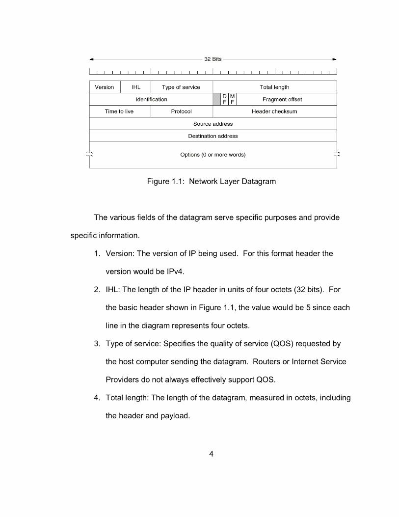
Figure 1.1 presents the structure of the datagram header that precedes

the data to be transmitted. In its most basic form, the header is comprised of 20

octets. There are optional fields that can be appended to the basic header that

offer additional capabilities. However, they are not relevant to the VoIP

transmission studied in this research.

4

Figure 1.1: Network Layer Datagram

The various fields of the datagram serve specific purposes and provide

specific information.

1. Version: The version of IP being used. For this format header the

version would be IPv4.

2. IHL: The length of the IP header in units of four octets (32 bits). For

the basic header shown in Figure 1.1, the value would be 5 since each

line in the diagram represents four octets.

3. Type of service: Specifies the quality of service (QOS) requested by

the host computer sending the datagram. Routers or Internet Service

Providers do not always effectively support QOS.

4. Total length: The length of the datagram, measured in octets, including

the header and payload.

5

5. Identification: As well as handling the addressing of datagrams

between two computers or hosts, IP needs to handle the splitting of

data payloads into smaller packages. This process, known as

fragmentation, is required since lower link layer protocols such as

Ethernet cannot always handle large packet sizes even though a single

IP datagram can handle a theoretical maximum length of 65,515

octets. This field is a unique reference number assigned by the

sending host to aid in the reassembly of a fragmented datagram.

6. Flags: Flags indicate whether the datagram may be fragmented and if

it has been fragmented, whether further fragments follow the current

fragment.

7. Fragment offset: This field indicates where this fragment belongs in the

datagram. It is measured in units of 8 octets or 64 bits.

8. Time to live: This field indicates the maximum time the datagram is

permitted to remain in the Internet system. This parameter ensures

that a datagram that cannot reach its destination host is given a finite

lifetime.

9. Protocol: This field indicates the higher-level protocol in use for this

datagram. Numbers have been assigned for use with this field to

represent such transport layer protocols as TCP and UDP.

10. Header checksum: This is a checksum covering the header only.

6

11. Source address: The IP address of the host that generated this

datagram. IPv4 addresses are 32 bits in length. When written or

spoken a dotted decimal notation is used (e.g.: 192.168.0.1).

12. Destination address: The IP address of the destination host. This is the

last field of the datagram.

1.1.2 Transport Layer

Generally, there are two protocols available at the transport layer when

transmitting information through an IP network. These are the Transmission

Control Protocol (TCP) and the User Datagram Protocol (UDP). These protocols

enable the transmission of information between the correct processes or

applications on host computers. These processes are associated with unique

port numbers. For example, the HTTP application is usually associated with port

80.

TCP is a connection-oriented protocol. Therefore, TCP establishes a

communications path prior to transmitting data and handles sequencing and error

detection, which ensures that a reliable stream of data is received by the

destination application.

Voice is a real-time application and mechanisms must be in place to

ensure that information is reliably received in the correct sequence and with

predictable delay characteristics. Although TCP would address these

requirements to a certain extent, there are some functions, which are reserved

7

for the layer above TCP. Therefore, for the transport layer, TCP is not used and

the alternative protocol, UDP, is commonly used.

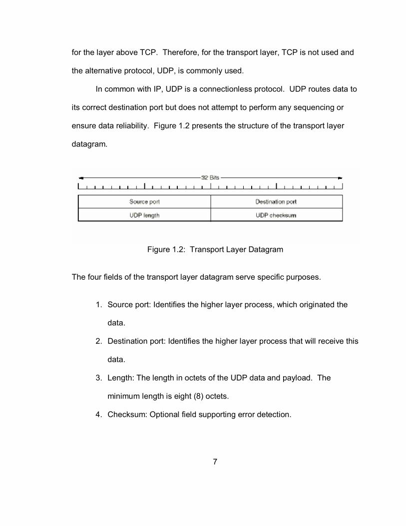
In common with IP, UDP is a connectionless protocol. UDP routes data to

its correct destination port but does not attempt to perform any sequencing or

ensure data reliability. Figure 1.2 presents the structure of the transport layer

datagram.

Figure 1.2: Transport Layer Datagram

The four fields of the transport layer datagram serve specific purposes.

1. Source port: Identifies the higher layer process, which originated the

data.

2. Destination port: Identifies the higher layer process that will receive this

data.

3. Length: The length in octets of the UDP data and payload. The

minimum length is eight (8) octets.

4. Checksum: Optional field supporting error detection.

8

1.2 Motivation

In a Voice over IP, (VoIP), application, the voice is digitized and

packetized at the sending facility at regular intervals, (e.g., every 10 ms), using

an encoding algorithm. Then the voice packet is sent over the IP network to the

receiver where it is decoded and played-out to the listener.

These voice packets are typically transported over an IP using the User

Datagram Protocol (UDP). The UDP, unlike the Transmission Control Protocol,

(TCP), does not have provisions for retransmission of lost packets. Lost packets

are packets that do not arrive at the proper time or at any receiver. For this

reason, UDP is characterized as a send and pray, (SNP), protocol. IP networks

such as the Internet are inherently best effort networks with variable delay and

loss.

The question is often asked. “Why not use TCP instead of UDP for the

transmission on voice packets?” The simple reason is that, in the case of voice

packets, “never” is significantly better than “late” for lost packets. By the time a

lost packet is detected and retransmitted the delay is more than sufficient to

render the voice packet useless. Therefore, a good concealment algorithm

needs to be designed for lost packets.

Packet loss tends to be a major cause of lost voice signals. It arises

primarily from network congestion. Voice traffic can tolerate some packet loss.

However, if the packet loss rate is greater than 5% it is considered harmful to the

voice quality and a good concealment technique is required for reconstruction of

9

the lost packets. In this research an effort was directed to the development of a

concealment algorithm that would maintain the quality of voice for lost packets.

Chapter 2 details the process of pitch detection, which is essential for a

good concealment algorithm. Afterwards, some existing concealment techniques

are explored. Then the new algorithm for packet loss concealment is introduced.

Test results for the algorithm are given in the last chapter.

10

CHAPTER 2

PITCH DETECTION

The main work of this research consisted of developing an improved

packet loss concealment algorithm based on time-scale modifications of speech.

Existing time-scale modification algorithms did not take the pitch period of the

speech signal waveform into consideration. As will be shown later, taking into

consideration the pitch of the speech signal and modifying the existing time scale

yields a much better quality for the reconstructed speech signal. Thus pitch

detection for the signal is important. This chapter presents and explains an

algorithm for pitch detection.

2.1 Introduction

A speech signal is passed through a low pass filter before pitch detection

is performed. The low pass filtered speech signal is sampled at 8KHz and then

quantized using a 16-bit quantizer. The digitized speech signal X(n) is processed

as 20ms frames and a Linear Predictive Coding (LPC) error signal e(n)

generated using a 10th order LPC analyzer. The signal, which is sampled at

8KHz and processed as 20ms frames, yields 160 sample points per frame.

11

2.1.1 Quantization

Sampling takes a snapshot of the input signal at an instant of time. When

the snapshot is taken the sampled analog value must be converted to a binary

number. The conversion from infinitely precise amplitude to a binary number is

called quantization. During quantization the analog to digital converter uses a

finite number of evenly spaced values to represent the analog signal. The

number of bits used for the conversion determines the number of different values

possible. Most modern converters use 12 or 16 bits. Typically, the converter

selects the digital value that is closest to the actual sampled value. In Matlab a

function exists for implementing quantization. The function is named “Quant” and

digitizes values as multiples of a quantity. The syntax of “Quant” is quant(x, q),

where x and q are the inputs to the function. The variable x is a, scalar or

vector, matrix and the variable q is the minimum value. For example, if

x = [1.333 4.756 3.897] (2.1)

and

y = quant(x, 0.1) (2.2)

then

y=[1.3 4.8 3.9]. (2.3)

Thus x is rounded to the nearest multiple of q.

12

2.1.2 Linear Prediction Coefficients (LPC)

LPC is a method of separating out the effects of the source from a speech

signal. LPC can be thought of as a way of encoding the information in a speech

signal into a smaller space for transmission over a restricted channel. LPC

encodes a signal by finding a set of weights for earlier signal values that can

predict the next signal value. The next signal value is given by

y[n] = a[1]y[n - 1] + a[2]y[n - 2] + a[3]y[n - 3] + e[n]. (2.4)

If values for a[1], a[2] and a[3] can be found such that the error signal e[n]

is very small for a segment of speech, (for example, one frame), then only a[1],

a[2], a[3] need to be transmitted instead of the signal values in the window. The

speech frame can be reconstructed at the other end by using a default e[n] signal

and predicting subsequent values from earlier ones.

A function exists in Matlab for implementing LPC. The function is named

“lpc”. The function and the syntax is given by

A = LPC (X,N), (2.5)

where X is the signal whose linear prediction coefficients needs to be found and

N is the order or the number of coefficients. A is represented by

A = [1, A(2), ..., A(N+1)]. (2.6)

The pitch information is present in both the original digitized signal X(n) and the

error signal e(n). Therefore, pitch detection is performed on both signals.

Typically, any periodicity that appears in the original signal X(n) also appears in

13

the error signal. However, as shown in later examples, several cases exist

where pitch detection needs to be performed on both signals.

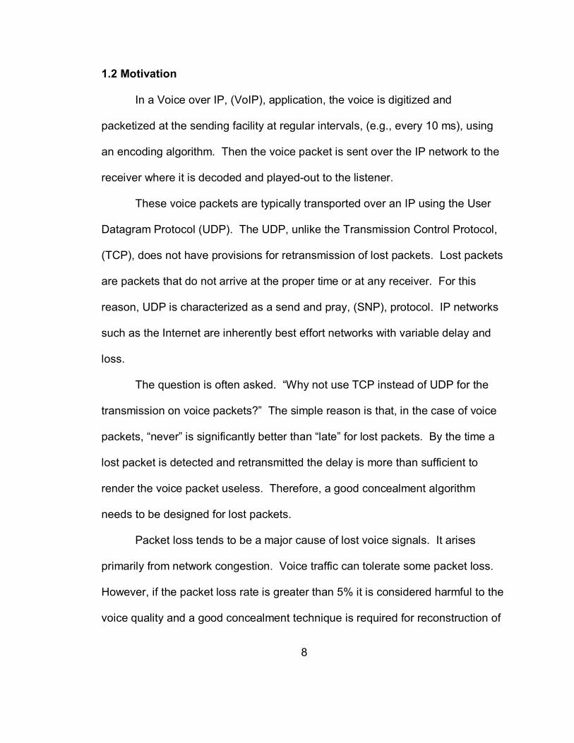
As shown in Figure 2.1, a particular formant structure in the waveform

causes the periodicity of the waveform to be obscure. When a person is

speaking the variations produced in the speech signal by acts such as opening

the teeth or rounding the lips causes the frequency response of the speech

signal to have several peaks. These peaks are known as formants. Since the

LPC residual signal e(n) represents the speech waveform with the formant

structure removed, pitch detection performed on e(n) provides a correct estimate

of the pitch.

Figure 2.1: Speech Waveform Shows Lack of Clear Periodicity Due to Formants

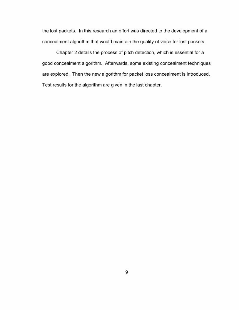
Another case arises when the residual waveform fails to show clear

periodicity in voiced frames. This condition is presented in Figure 2.2. Such a

situation occurs when the fundamental frequency of the excitation information,

which is found in the residual, is removed by LPC inverse filtering. The inverse

filtering causes the residual to look noisy while the original speech signal appears

to be clearly periodic.

14

Figure 2.2: LPC Residual Shows Lack of Clear Periodicity

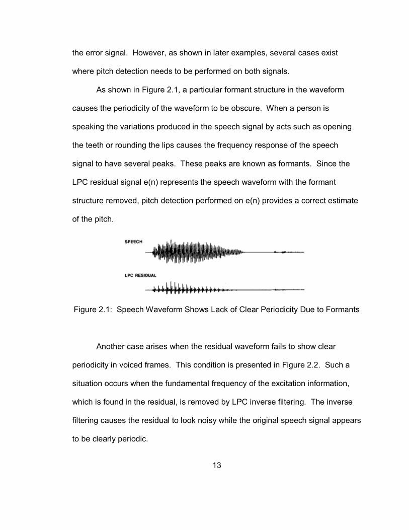
Once the LPC error signal is generated, the LPC error signal e(n) and the

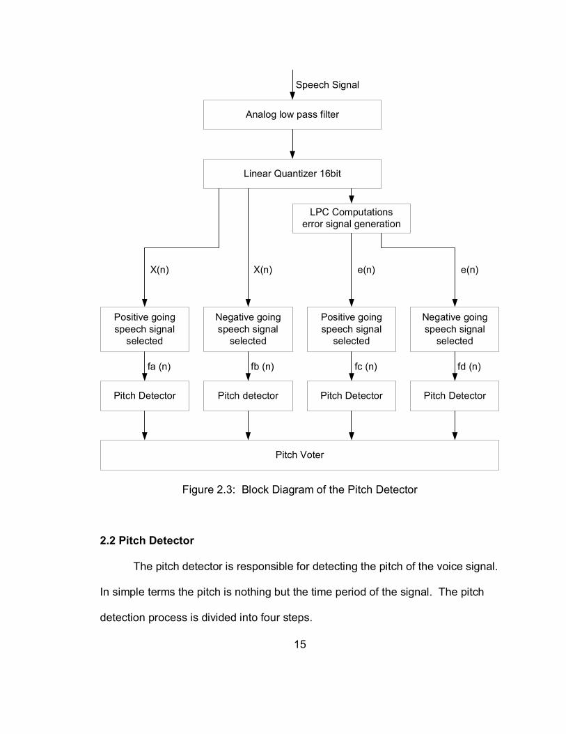
digitized speech signal X(n) is split into positive going and negative going signals.

The resulting four signals are positive going X(n), negative going X(n), positive

going e(n) and negative going e(n). These signals are named fa(n), fb(n), fc(n)

and fd(n) respectively. Pitch detection analysis is performed on each of these

signals individually by four pitch detectors that operate in parallel. The structure

of the pitch detectors is identical. The pitch detector structure is described in the

next section and differences occur only in the values of their control parameters.

The pitch voter combines the four pitch detection estimates to produce a final

pitch estimate. Figure 2.3 presents a block diagram of the entire process.

15

Analog low pass filter

Speech Signal

Linear Quantizer 16bit

LPC Computationserror signal generation

Positive goingspeech signal

selected

Negative goingspeech signal

selected

Positive goingspeech signal

selected

Negative goingspeech signal

selected

X(n) X(n) e(n) e(n)

Pitch Detector Pitch DetectorPitch DetectorPitch detector

Pitch Voter

fa (n) fd (n)fc (n)fb (n)

Figure 2.3: Block Diagram of the Pitch Detector

2.2 Pitch Detector

The pitch detector is responsible for detecting the pitch of the voice signal.

In simple terms the pitch is nothing but the time period of the signal. The pitch

detection process is divided into four steps.

16

1. Find a set of candidate pulses.

2. Find a subset of the set of candidate pulses such that a candidate

distance (DC) separates all the selected pulses.

3. Perform linear interpolation on the selected pulses.

4. Perform a Pitch consistency test.

Each of these steps is described along with a flowchart and an algorithm of how

this process is implemented in Matlab.

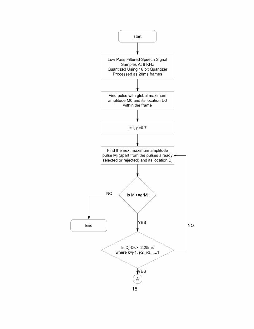
2.2.1 Finding a Set of Candidate Pulses

The operation starts by identifying a set of samples, called a Candidate

Pulse Set, over a frame on which the pitch or periodicity is to be detected. In

order to find these pulses the global maximum amplitude, M0, is found. M0 is the

sample or pulse that has the highest amplitude among all the samples in the

frame. Its location within the frame is D0. This global maximum is the first

sample that enters the set of candidate pulses. All pulses selected after M0 must

satisfy three conditions.

1. First: The next pulse selected must be a local maximum, which means it

must have the maximum amplitude after excluding the pulses that have

already been selected. This selection is reasonable since pitch pulses

normally have amplitudes higher than any other pulses in the frame. Mj

denotes the amplitude of this local maximum and its location within the

frame is denoted by Dj.

17

2. Second: Any selected pulse must have amplitude at least equal to a

fraction of the global maximum amplitude M0. That is

3. Mj >= g*M0, (2.7)

where g is called the threshold amplitude percentage. The value of g is

normally set between 0.175 and 0.525 for a good pitch estimate.

4. Third: All the selected pulses must be separated by at least 2.25ms, which

is 18 sample periods from all other selected pulses. The reason for

including this condition is that the largest human speech frequency

encountered is 400Hz. A frequency of 400Hz corresponds to a time

period of 2.55ms. Therefore, the smallest human speech pitch is 2.55ms.

If a small tolerance level, of approximately 10%, is allowed, it is only

necessary for the selected pulses to be separated by 2.25 ms. Figure 2.4

presents a block diagram of the entire process.

18

start

Find pulse with global maximumamplitude M0 and its location D0

within the frame

Low Pass Filtered Speech SignalSamples At 8 KHz

Quantized Using 16 bit QuantizerProcessed as 20ms frames

j=1, g=0.7

Find the next maximum amplitudepulse Mj (apart from the pulses alreadyselected or rejected) and its location Dj

Is Mj>=g*Mj

YES

NO

End

Is Dj-Dk>=2.25mswhere k=j-1, j-2, j-3......1

NO

A

YES

19

Add selected pulse's amplitude andlocation to candidate pulse set

CANDIDATE PULSES

YES

A

end

Figure 2.4: Flowchart For Finding a Set of Candidate Pulses

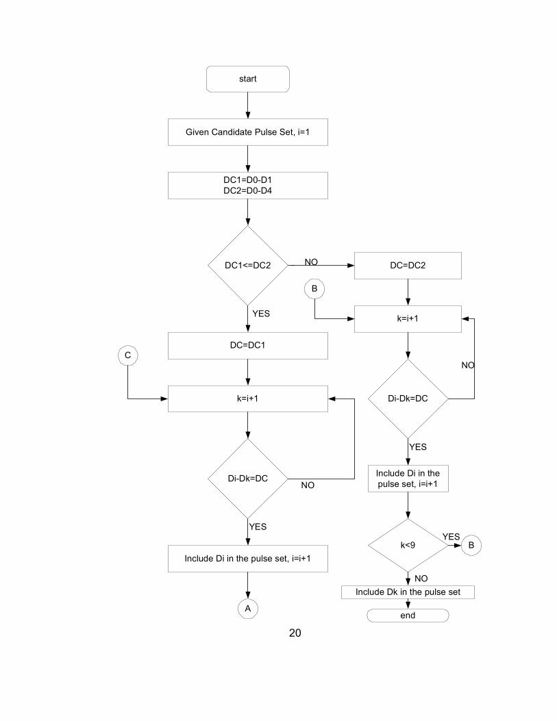
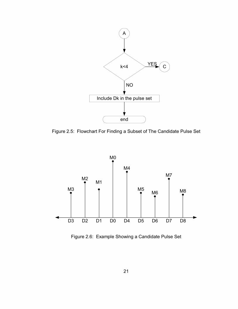
2.2.2 Finding a Subset of the Set of Candidate Pulses

The candidate pulse set consists of pulses with amplitudes Mj and

locations Dj. These amplitudes and their locations are used to find a distance

that is the smallest distance over which a subset of these pulses is periodic. The

periodic distance is determined recursively by considering the distance from the

global framing maximum M0 to the closest adjacent pulse. This distance is

called the candidate distance (DC) and is given by

DC = |D0 – Dj| (2.8)

If this distance does not separate a subset of maxima in the frame, plus or minus

a breathing threshold B, then the candidate distance is discarded and the

process begins again with the next closest adjacent candidate pulse. Figure 2.5

flowcharts the process of finding a subset of the candidate pulse set. Figure 2.6

presents an example set of candidate pulses.

20

start

Given Candidate Pulse Set, i=1

DC1=D0-D1DC2=D0-D4

DC1<=DC2

DC=DC1

YES

DC=DC2NO

k=i+1

Di-Dk=DCNO

YES

k=i+1

Di-Dk=DC

YES

NO

Include Di in the pulse set, i=i+1

Include Di in thepulse set, i=i+1

k<9YES

B

A

B

C

NOInclude Dk in the pulse set

end

21

A

k<4

end

Include Dk in the pulse set

CYES

NO

Figure 2.5: Flowchart For Finding a Subset of The Candidate Pulse Set

D0D1D2D3 D7D6D5D4 D8

M8

M7

M6M5

M4

M0

M1M2

M3

Figure 2.6: Example Showing a Candidate Pulse Set

22

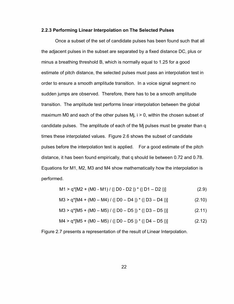
2.2.3 Performing Linear Interpolation on The Selected Pulses

Once a subset of the set of candidate pulses has been found such that all

the adjacent pulses in the subset are separated by a fixed distance DC, plus or

minus a breathing threshold B, which is normally equal to 1.25 for a good

estimate of pitch distance, the selected pulses must pass an interpolation test in

order to ensure a smooth amplitude transition. In a voice signal segment no

sudden jumps are observed. Therefore, there has to be a smooth amplitude

transition. The amplitude test performs linear interpolation between the global

maximum M0 and each of the other pulses Mj, i > 0, within the chosen subset of

candidate pulses. The amplitude of each of the Mj pulses must be greater than q

times these interpolated values. Figure 2.6 shows the subset of candidate

pulses before the interpolation test is applied. For a good estimate of the pitch

distance, it has been found empirically, that q should lie between 0.72 and 0.78.

Equations for M1, M2, M3 and M4 show mathematically how the interpolation is

performed.

M1 > q*[M2 + (M0 - M1) / (| D0 - D2 |) * (| D1 – D2 |)] (2.9)

M3 > q*[M4 + (M0 – M4) / (| D0 – D4 |) * (| D3 – D4 |)] (2.10)

M3 > q*[M5 + (M0 – M5) / (| D0 – D5 |) * (| D3 – D5 |)] (2.11)

M4 > q*[M5 + (M0 – M5) / (| D0 – D5 |) * (| D4 – D5 |)] (2.12)

Figure 2.7 presents a representation of the result of Linear Interpolation.

23

D0D1D2 D4D3

M4

M3

M0

M1M2

D5

M5

DCDC DC DC DC

Figure 2.7: Linear Interpolation

The interpolation is performed with respect to all the pulses following a

particular pulse in a particular direction. If the subset of the candidate pulse set

passes the interpolation test, then it contains a valid set of pulses and DC is a

valid pitch distance. If any of the above equations fails to provide a valid result

then the DC is not valid and must be computed again from the previous process

of finding a subset of the set of candidate pulses.

2.2.4 Pitch Consistency Test

If a pitch DC estimate is found over two consecutive frames T(i) and T(i -

1) then the two estimates must be consistent with each other such that

|T(i - 1) – T(i)| <= A, (2.13)

where A is the pitch threshold. If the pitch threshold is valid then the DC is a

good estimate of the pitch distance. If the calculation, for pitch threshold, in

24

Equation (2.13) is not valid then and a new pitch threshold is calculated in

accordance with Equation (2.14), which is given by

|T(i - 1) – 2*T(i)| <= A. (2.14)

Equation (2.14) corrects any pitch doubling error that might have occurred. If

neither Equation (2.13) nor Equation (2.14) is valid then a new candidate

distance must be calculated. The best value for pitch threshold A is 1.25 ms.

The algorithm presented in this chapter for pitch detection proves to be a

very effective and accurate algorithm. The pitch value detected was used in the

packet loss concealment algorithm that was developed for this research. The

packet loss concealment algorithm is discussed in Chapter 3.

25

CHAPTER 3

PACKET LOSS CONCEALMENT

In this research, Time Scale Modification, (TSM), of speech was used to

conceal lost packets in a voice packet stream. TSM is traditionally used to alter

the rate of a signal in order to either expand or compress the signal.

3.1 Time Scale Modification of Speech

TSM is the process of changing the perceived rate of articulation of

speech. It is a process of compressing, hastening, or expanding, slowing down,

the time scale of an audio segment. A signal, which is time scale compressed

has shorter duration while a signal, which is time scale expanded has a longer

duration. Uses of time scale compression are fast listening of messages on

answering machines, voice mail systems or synchronizing speech with the typing

speed for dictation. Similarly a simple use of time scale expansion or slowing

down speech is that it helps in the comprehension of rapidly spoken speech

segments.

As stated earlier, Time Scale Modification of the speech signal is required

in order to conceal packet loss in a voice stream. Thus Time Scale Modification

should keep the principal characteristics of speech such as timbre, pitch and

26

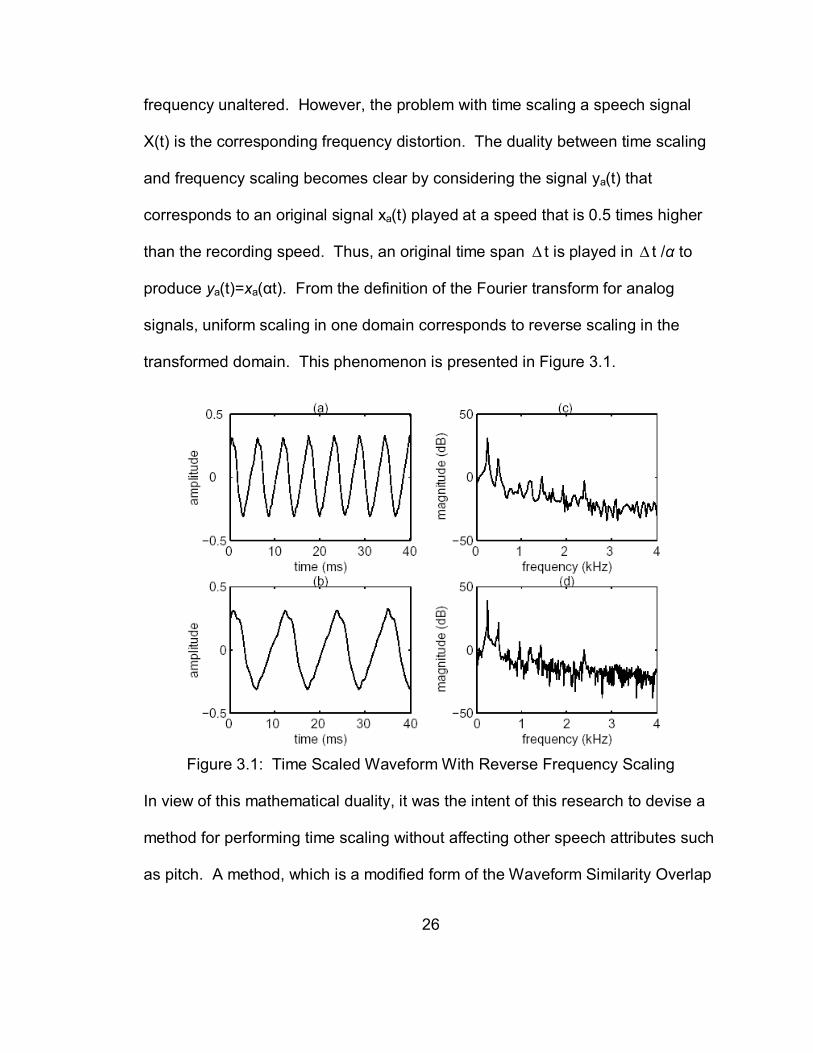
frequency unaltered. However, the problem with time scaling a speech signal

X(t) is the corresponding frequency distortion. The duality between time scaling

and frequency scaling becomes clear by considering the signal ya(t) that

corresponds to an original signal xa(t) played at a speed that is 0.5 times higher

than the recording speed. Thus, an original time span ∆ t is played in ∆ t /α to

produce ya(t)=xa(αt). From the definition of the Fourier transform for analog

signals, uniform scaling in one domain corresponds to reverse scaling in the

transformed domain. This phenomenon is presented in Figure 3.1.

Figure 3.1: Time Scaled Waveform With Reverse Frequency Scaling

In view of this mathematical duality, it was the intent of this research to devise a

method for performing time scaling without affecting other speech attributes such

as pitch. A method, which is a modified form of the Waveform Similarity Overlap

27

Add, (WSOLA), algorithm was devised to achieve the objective. The next

sections discuss existing methods, including conventional WSOLA, for Time

Scale Modification.

3.2 Short Time Fourier Transform (STFT)

The Fourier Transform is the most commonly used frequency domain

representation of signals in signal processing. The Discrete Fourier Transform is

defined as follows

∑+∞=

−∞=

ω−=+ n

n

nje)n(x)jωe(X (3.1)

Speech evolves slowly. Therefore, if a short time analysis strategy is used along

with the Fourier Transform a Short Time Fourier Transform is obtained. A short

time strategy implies segmenting the signal and applying the Fourier Transform

to the segments. Segmenting is achieved by windowing. A common window

function that is used is the Hamming window. A mathematical definition of the

STFT is developed as follows. Signal x(n) is segmented using windowing

function w(n)

Xω(n, m)=ω(n) x(n +m) (3.2)

Next the Fourier transform is applied to obtain

∑+∞=

−∞=

ω−ω+=ωn

n)nje()mn(x)m,(X , (3.3)

28

which is the Short Time Fourier Transform representation. Since windowing is

used, the precision of the Fourier Transform is limited. However, the STFT

works well for consecutive overlapping signal segments.

The Short Time Fourier Transform is the basic mathematical tool that is

applied for implementation of packet loss concealment. Two techniques that are

presently used are first discussed. They also form the basis for the technique

implemented in this research. The two methods are termed Overlap Add, (OLA),

and Synchronization Overlap Add, (SOLA).

3.3 Packet Loss Concealment

In an audio communication system speech in encoded and packetized at

the transmitter, sent over a network and then decoded at the receiver. Packet

loss concealment algorithms are needed to conceal the packets of the speech

signal that are lost during transmission. The basic function of these algorithms is

to generate a synthetic speech signal to cover the missing speech packets.

There are basically two types of techniques. These techniques are termed

transmitter based and receiver based techniques for packet loss concealment.

The techniques described in this chapter are receiver based and are applicable

to the ITU recommendation G.711. G.711, unlike some CELP based coders,

does not have built-in packet loss concealment algorithms so a receiver-based

algorithm is required. One advantage of G.711 is that the signal returns to its

original form immediately after a missing packet. With CELP based coders the

signal takes time to recover after a missing packet.

29

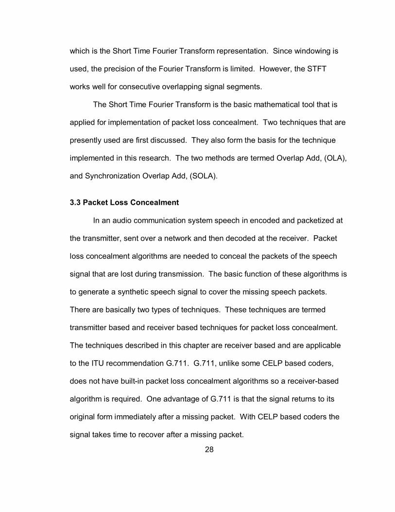
Time Scale Modification techniques for speech signals are used to cover

up the missing packets at the receiver end. In simple terms the packets that

precede the lost packets are stretched in time to cover up the length of the

missing packets. This action is presented in figure 3.2. In Figure3.3 three

preceding packets are stretched to make up for the loss of one packet. As

shown packet 2 is lost during transmission and Time Scale Modification is

performed on packets 3, 4 and 5 in order to cover the missing packet.

The next sections deal with some of the existing packet loss concealment

techniques and section 3.7 introduces the modified WSOLA technique of packet

loss concealment by Time Scale Modification.

0 20 40 60 80 100 120

1 2 3 4 5 6

0 20 40 60 80 100 120

1 3 4 5 6

Time (ms)

Time (ms)

Figure 3.2: Lost Packet Reconstructed Using Two Previously Received Packets

30

3.4 Overlap-Add Synthesis Method

Considering a signal x(n) and performing a STFT on it produces a

transformed signal X(n,m) as discussed in section 3.2. If this signal is modified

to achieve time scaling, another signal Ŷ(w,n) is produced that is different from

x(n) when the inverse STFT performed. In fact, Ŷ(w,n) may not even have an

inverse STFT. However, this time scaled signal will contain information that best

characterizes the signal modification. A synthesis formula that provides a correct

value of Ŷ(w,n) such that it’s inverse STFT is valid was derived by using the least

mean squared error technique. In this method y(n), the inverse STFT of Y(w,n),

is constructed such that Ŷ(w,n) is maximally close to Ŷ in the mean square error

sense. The mean square error

∑ ∫+− ωω−ωΠ

= ΠΠk d2|)k,(Y)k,(Y|

21E (3.4)

is minimized over all signals y(n). Parseval’s theorem allows equation 3.4 to be

written as

∑ ∑+∞=

−∞=ω+−ω= k

m

m2))m()km(y)k,m(y(E (3.5)

The signal y(n) which minimizes E is obtained by solving

∑ =−ω−ω−−ω−=∂∂k

0)kn())kn()n(y)k,kn(y(2)n(y/E , (3.6)

which yields

∑ −ω

∑ −ω−ω=

k)kn(2

k )k,kn(y)kn()n(y . (3.7)

31

The OLA synthesis formula reconstructs the original signal if X(ω,m) is a

valid STFT or a signal whose STFT is maximally close to X(ω,m) in the least

squares sense is constructed. Furthermore, the denominator in equation 3.7 is

required only to compensate for a possible non-uniform weighting of samples in

the windowing procedure. The synthesis operation can be simplified if the

windowing function and the synthesis time instants k can be chosen such that

1)kn(2k

=−ω∑ (3.8)

A common choice in speech processing, that satisfies this simplifying condition,

is the choice of a Hanning window with 50% overlap between successive

segments.

The OLA synthesis yields a close realization of the time-scale modification in the

time domain. By adopting a short-time analysis strategy for constructing X(ω,m)

and by using the OLA criteria for synthesizing a signal y(n) from the modified

representation

Ŷ(ω,m) = Mxy[X(ω,m)] (3.9)

will always provide modification algorithms that can be operated in the time

domain if the modification operator Mxy [.] works only on the time index m such

that

Ŷ(ω,m) = X(ω,Mxy[m]). (3.10)

Taking the inverse Fourier transform yields

Ŷ(ω,m) = Xω(n,Mxy[m]). (3.11)

Combining equation (3.7) and equation (3.11) yields

32

∑∑

−ω

−−ω=

ω

m

2m

xy

)mn(

])m[M,mn(x)mn()n(y . (3.12)

It is clear from the equation (3.12) that modification is obtained by excising

segments xω(n,Mxy[m]) from the input signal by using the window and repositions

them along the time axis before constructing the output signal by the weighted

overlap-addition of the segments. However, the periodicity of the time-scale

modified signal, presented in Figure 3.3(b), is changed from the original signal,

presented in Figure 3.3(a), if the above formula is applied to the time warping,

τ(m), of a signal. In general, poor results are obtained when using

Ŷ(ω,m) = X(ω, τ-1(m)). (3.13)

Figure 3.3: Periodicity Change

3.5 The Synchronized Overlap Add Method

Roucos and Wilgus developed the Synchronized Overlap-Add (SOLA)

algorithm. They sought to accomplish Time Scale Modification by providing the

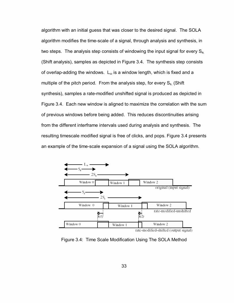
33

algorithm with an initial guess that was closer to the desired signal. The SOLA

algorithm modifies the time-scale of a signal, through analysis and synthesis, in

two steps. The analysis step consists of windowing the input signal for every Sa,

(Shift analysis), samples as depicted in Figure 3.4. The synthesis step consists

of overlap-adding the windows. Lω is a window length, which is fixed and a

multiple of the pitch period. From the analysis step, for every Ss, (Shift

synthesis), samples a rate-modified unshifted signal is produced as depicted in

Figure 3.4. Each new window is aligned to maximize the correlation with the sum

of previous windows before being added. This reduces discontinuities arising

from the different interframe intervals used during analysis and synthesis. The

resulting timescale modified signal is free of clicks, and pops. Figure 3.4 presents

an example of the time-scale expansion of a signal using the SOLA algorithm.

Figure 3.4: Time Scale Modification Using The SOLA Method

34

In the “Synchronized Overlap-Add” algorithm, windows are added

synchronously with the local period. The time-scale modified signal, y(n), which

is obtained from the “Synchronized Overlap-Add” of windowed segments is given

by xω(n) = ω(n)x(n), where x(n) is the input signal and ω(n) is the window

function, is given by:

1. Initializing the signals yω (n) and r(n):

yω(n) = xω(n); for n = 0,···,Lω – 1 (3.14)

r(n) = ω(n); for n = 0,···,Lω – 1 (3.15)

2. Updating yω(n) and r(n) by each new frame of the input signal, xω(n), is

effected as·follows

yω(mSs – k(m) + j) = yω(mSs – k(m) + j) + xω(mSa + j) for 0 <= j <= Lm –1

yω(mSs – k(m) + j) = xω( mSa + j) for Lm <= j <= Lω –1 (3.16)

where Lm is the number of overlapping points between the new window

xω(mSa+j) and the existing sequence yω (mSs – k (m) + j) for the current frame m.

r(mSs – k(m) + j) = r(mSs – k(m) + j) + ω(mSa + j) for 0 <= j <= Lm –1

r(mSs – k(m) + j) = ω(mSa + j) for Lm <= j <= Lω –1 (3.17)

k(m) = max )(kRmxy (3.18)

+

+−

++−=

∑∑

∑−

=ω

=ω

ωω

−

=

1Lm

0ja

21-Lm

0js

2

as

1L

0jmxy

)jmS(x)jkmS(y

)jmS(x)jkmS(y)k(R

m

(3.19)

3. Normalizing yw(n) by the buffer of appropriately shifted windowing functions

r(n) to obtain the final output y(n) yields

35

)j(r)j(y)j(y ω= for all j. (3.20)

As outlined in the above equations, k(m) > 0 corresponds to a shift

backwards along the time-axis of the mth frame that maximizes the normalized

cross correlation )k(Rmxy between the mth window and the rate-modified shifted

signal composed of windows 0 to window (m-1). Lω is the number of data points

in each window frame xω(mSa + j). Maximizing the cross-correlation insures the

current window is added and averaged with the most similar region of the

reconstructed signal as it exists at that point. The shifting operation insures that

the largest amplitude periodicity of the signal will be preserved in the rate-

modified signal. The resulting signal is called the rate-modified shifted signal to

distinguish it from the rate-modified unshifted signal, which is obtained simply by

overlap adding (see Figure 3.4).

It is known that the straightforward OLA synthesis from the time-scaled

and down sampled STFT

Ŷ (ω, kS) = X (ω, τ-1(kS)) (3.21)

results in a signal

∑∑

−ω

τ+−−ω=

−

k

2k

12

1 )kSn(

))kS(kSn(x)kSn()n(y (3.22)

that is heavily distorted, as illustrated in Fig 3.3. In equation (3.22), ‘S’ is a down

sampling factor introduced to reduce the amount of information that needs to be

processed. In order to avoid pitch period discontinuities or phase jumps at

36

waveform-segment joins, each input segment needs to be realigned to the

already formed portion of the output signal before performing the OLA operation.

Thus, the synchronized OLA algorithm produces the time-scale modified signal

∑∑

∆+−

∆+τ+−∆+−=

−

k

k

1

)kkSn(v

)k)kS(kSn(x)kkSn(v)n(y (3.23)

in a left-to-right fashion with a windowing function v(n) and a shift factor ∆k

belonging to the set [-∆max ··· +∆max] that is chosen to maximize the cross-

correlation coefficient between the current segment

v(n-kS+∆k) x(n+τ-1(kS)-kS+∆k) (3.24)

and the already formed portion of the output signal

∑

∑−

−∞=

−

−∞=

−

∆+−

∆+−τ+∆+−=− 1k

l

1k

l

1

)tlSn(v

)tlS)lS(n(x)tlSn(v)1k;n(y . (3.25)

SOLA is computationally efficient since it requires no iterations and can be

operated in the time domain. The time domain operation implies that the

corresponding STFT modification affects the time axis only. Application of

SOLA, yields

Ŷ(ω,kS-∆k) = X(ω,τ-1(kS)). (3.26)

The shift parameter ∆k implies a tolerance on the time warp function. However,

in order to ensure a synchronized overlap-addition of segments, the desired time

warp function, τ(n), is not realized exactly. A deviation on the order of a pitch

period is allowed.

37

3.6 Waveform Similarity Overlap Add (WSOLA)

Further enhancement of the SOLA algorithm is the (WSOLA) technique. It

considers that a time-scaled version of an original signal should be perceived to

consist of the same acoustic events as the original signal but with these events

being produced according to a modified timing stricture. In WSOLA, this can be

achieved by constructing a synthetic waveform y(n) that maintains maximal local

similarity to the original waveform x(m) in all neighborhoods of related sample

indices m= 1−τ (n). Using the symbol ‘ ⇔ ’ to denote “the maximal similarity” and

using the window ω(n) to select such neighborhoods

y(n+m) ω(n) ⇔ x(n+ 1−τ (m) + ∆m)ω(n) (3.27)

Ŷ(ω,m) ⇔ X(ω, 1−τ (m) + ∆m) (3.28)

Comparing equations (3.27) and 3.28 yields an alternative interpretation for the

timing tolerance parameters ∆k since the waveform similarity criterion and the

synchronization problem are closely related. As shown in the above equations,

the ∆m was introduced in order to obtain a meaningful formulation of the

waveform similarity criterion since two signals need to be considered as identical

if they only differ by a small time offset.

3.6.1 Practical Implementation of WSOLA

Analysis segment size, (Ss), is fixed irrespective of the input speech

characteristics. Time scale factor alpha is set to less that 1 depending on the

38

desired expansion. Overlap segment size, (S0), is computed as 0.5 times Ss

and is fixed. Once these parameters are fixed the output signal is formed from

the input speech signal. The first two iterations for the procedure are depicted in

Figure 3.5.

During the first iteration the first Ss samples of the input are directly copied

to the output. If1 denotes the index of the last sample of the output and overlap

index O1 is determined as S0 samples from the end of the last available samples

of the output. The samples of the output between If1 and O1 are the ones that

are overlap added. The first search index, (S1), is determined as alpha times

O1. This search index is marked on the input signal and a search window is

determined. The search window consists of samples around S1. Once within

the window the best cross correlating samples are determined using the cross

correlation equation

2/10

0

0

0

22

0

0

))()((

)()()(

∑ ∑

∑=

=

=

=

=

=

+++

+++=

Sj

j

Sj

j

Sj

j

jOiYkjSiX

jOiYkjSiXKR (3.29)

where K=Si – Loff to Si + Hoff. Loff and Hoff are both 10 samples each. The

maximum m is k=m where normalized R(k) is maximum. The best index B1 is

determined as (S1+m).

Using equation (3.29) the beginning of the best correlating samples is

determined as index B1 and is marked in the input as shown in Figure 3.5. Next

the S0 samples beginning at B1 are multiplied by an increasing ramp function,

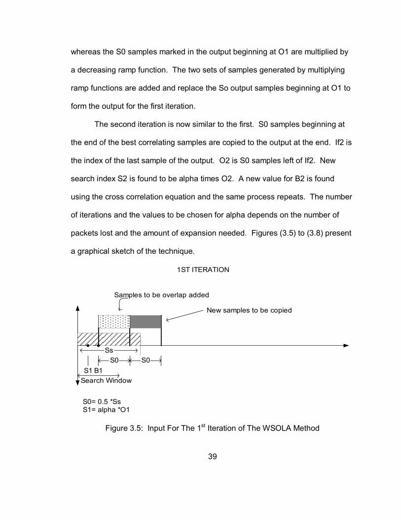
39

whereas the S0 samples marked in the output beginning at O1 are multiplied by

a decreasing ramp function. The two sets of samples generated by multiplying

ramp functions are added and replace the So output samples beginning at O1 to

form the output for the first iteration.

The second iteration is now similar to the first. S0 samples beginning at

the end of the best correlating samples are copied to the output at the end. If2 is

the index of the last sample of the output. O2 is S0 samples left of If2. New

search index S2 is found to be alpha times O2. A new value for B2 is found

using the cross correlation equation and the same process repeats. The number

of iterations and the values to be chosen for alpha depends on the number of

packets lost and the amount of expansion needed. Figures (3.5) to (3.8) present

a graphical sketch of the technique.

Ss

S0= 0.5 *SsS1= alpha *O1

B1S1S0 S0

New samples to be copied

Samples to be overlap added

Search Window

1ST ITERATION

Figure 3.5: Input For The 1st Iteration of The WSOLA Method

40

Ss

S0

If1O1

New samples copied from Input

OUTPUT

S0

overlap added samples

1ST ITERATION

Figure3.6: Output For The 1st Iteration of The WSOLA Method

Ss

S2= alpha *O2

B1S1S0 S0

INPUT

2ND ITERATION

S2 B2S0 S0

Samples to be overlap added

New samples to be copied

Figure3.7: Input For The 2nd Iteration of The WSOLA Method

41

Ss

S0

If1O1

OUTPUT

S0

overlap added samples fromiteration 1

O2If2

overlap added samples

New samples copied from Input

2ND ITERATION

Figure3.8: Output For The 2nd Iteration of The WSOLA Method

3.6.2 Drawbacks of WSOLA

The Waveform Similarity Overlap Add technique has been discussed in

the above sections. It is now summarized with respect to the constraints

involved and the drawbacks of the method are discussed. Following sections

introduce a new modified technique that overcomes these drawbacks.

WSOLA and its constraints:

1. Analysis segment size (Ss) is fixed irrespective of the input speech

signal characteristics.

2. Time scale factor (alpha) is set to less that 1 to achieve the required

expansion.

3. Overlap segment size (S0) is 0.5 times Ss.

4. If1 is the index of the last sample of the output.

5. Overlap index (O1) is S0 samples to the left of If1.

42

Two major drawbacks exist for WSOLA that greatly affect the quality of

speech produced upon expansion of a speech signal. First, the analysis

segment size (Ss) is fixed irrespective of the input speech signal characteristics.

Therefore, the optimum quality of the time scale expanded signal is not obtained.

If Ss is too large for the input speech signal, the resultant speech upon

expansion includes echoes and reverberations. Second, the overlap segment

size if 0.5 times Ss. Therefore, the user does not have the flexibility, for a given

time scale factor, of design with respect to quality of speech and complexity of

computations for a given system that has restraints. If a particular system has

limitations with respect to processing power and memory a complicated algorithm

will not be processed efficiently and the quality produced by the processing

algorithm (speech quality) cannot be enhanced. Vice versa, a system with good

processing power and memory will handle a complex algorithm and speech

quality can be enhanced. With these issues in mind the WSOLA algorithm was

modified to overcome the drawbacks and provide a better quality output signal

for speech.

3.7 Modified WSOLA

The new algorithm was modified with respect to the analysis segment size

(Ss) and the degree of overlap (f) in order to overcome the drawbacks of WSOLA

mentioned previously.

43

The segment size (Ss) is computed as a function of the pitch period of the

input speech signal. If P is the pitch period of the input speech signal then,

depending on P, Ss is defined as follows:

For P > 60,

Ss = 2 * p. (3.30)

For 40 < P < 60,

Ss = 120. (3.31)

For P < 40,

Ss = 100. (3.32)

The overlap segment size (S0) is f times Ss where f is the degree of

overlap. The degree of overlap is chosen as a function of quality and complexity.

An f > 0.5 provides higher quality at the expense of more complexity while an

f < 0.5 provides reduced complexity at the cost of quality.

The other constraints remain the same as in the WSOLA method. However,

introducing these changes produced a higher quality speech signal. A

discussion of this effect is presented in the results chapter. The practical

implementation of the modified WSOLA technique is described next.

3.7.1 Practical Implementation of Modified WSOLA

As discussed earlier, the degree of overlap, (f), is chosen according to the

requirements of the system and user flexibility. Analysis segment size, (Ss), is

optimized to input speech characteristics, in particular the pitch, of the input

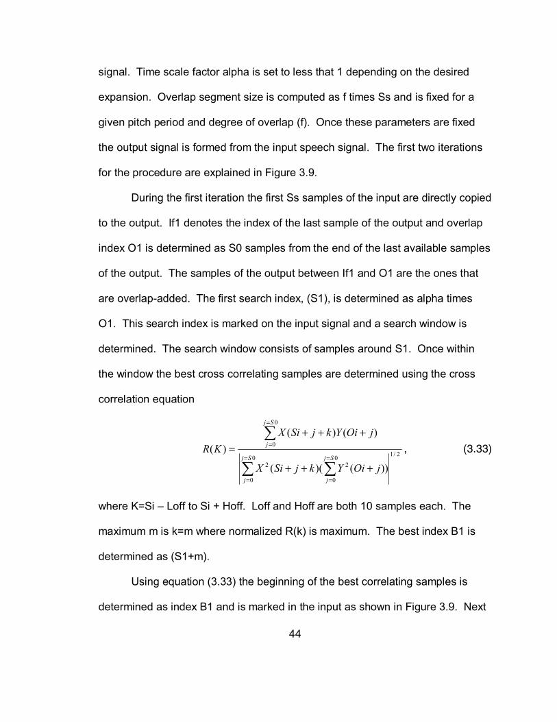
44

signal. Time scale factor alpha is set to less that 1 depending on the desired

expansion. Overlap segment size is computed as f times Ss and is fixed for a

given pitch period and degree of overlap (f). Once these parameters are fixed

the output signal is formed from the input speech signal. The first two iterations

for the procedure are explained in Figure 3.9.

During the first iteration the first Ss samples of the input are directly copied

to the output. If1 denotes the index of the last sample of the output and overlap

index O1 is determined as S0 samples from the end of the last available samples

of the output. The samples of the output between If1 and O1 are the ones that

are overlap-added. The first search index, (S1), is determined as alpha times

O1. This search index is marked on the input signal and a search window is

determined. The search window consists of samples around S1. Once within

the window the best cross correlating samples are determined using the cross

correlation equation

2/10

0

0

0

22

0

0

))()((

)()()(

∑ ∑

∑=

=

=

=

=

=

+++

+++=

Sj

j

Sj

j

Sj

j

jOiYkjSiX

jOiYkjSiXKR , (3.33)

where K=Si – Loff to Si + Hoff. Loff and Hoff are both 10 samples each. The

maximum m is k=m where normalized R(k) is maximum. The best index B1 is

determined as (S1+m).

Using equation (3.33) the beginning of the best correlating samples is

determined as index B1 and is marked in the input as shown in Figure 3.9. Next

45

the S0 samples beginning at B1 are multiplied by an increasing ramp function,

whereas the S0 samples marked in the output beginning at O1 are multiplied by

a decreasing ramp function. The two sets of samples generated by multiplying

by ramp functions are added and replace the S0 output samples beginning at O1

in order to form the output for the first iteration.

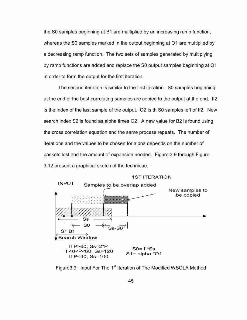
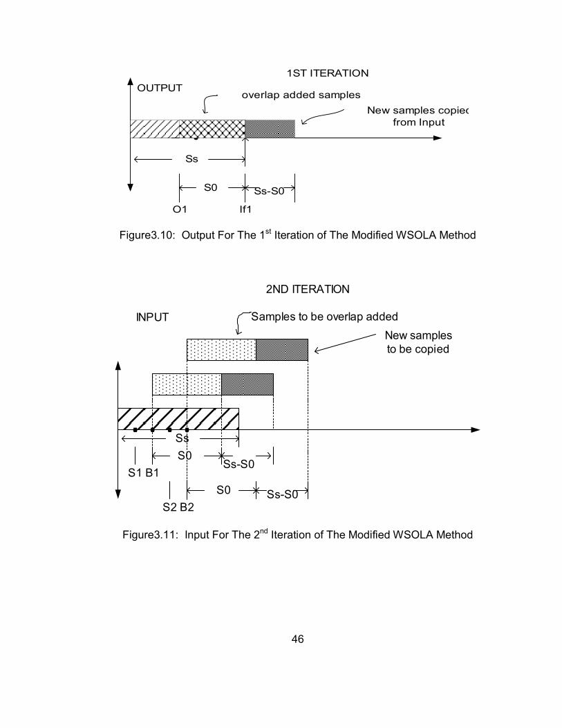
The second iteration is similar to the first iteration. S0 samples beginning

at the end of the best correlating samples are copied to the output at the end. If2

is the index of the last sample of the output. O2 is th S0 samples left of If2. New

search index S2 is found as alpha times O2. A new value for B2 is found using

the cross correlation equation and the same process repeats. The number of

iterations and the values to be chosen for alpha depends on the number of

packets lost and the amount of expansion needed. Figure 3.9 through Figure

3.12 present a graphical sketch of the technique.

If P>60; Ss=2*PIf 40<P<60; Ss=120

If P<40; Ss=100

Ss

S0= f *SsS1= alpha *O1

B1S1S0

Ss-S0

New samples tobe copied

Samples to be overlap added

Search Window

INPUT1ST ITERATION

Figure3.9: Input For The 1st Iteration of The Modified WSOLA Method

46

Ss

S0

If1O1

New samples copiedfrom Input

OUTPUToverlap added samples

Ss-S0

1ST ITERATION

Figure3.10: Output For The 1st Iteration of The Modified WSOLA Method

Ss

B1S1S0

Ss-S0

New samplesto be copied

Samples to be overlap addedINPUT

2ND ITERATION

S2 B2S0 Ss-S0

Figure3.11: Input For The 2nd Iteration of The Modified WSOLA Method

47

SsS0

If1O1

New samplescopied from Input

OUTPUT overlap added samples fromiterarion 2

Ss-S0

If2O2S0

Region of overlapbetween iteration

1 and 2

overlap added samples fromiterarion 1

Figure3.12: Output For The 2nd Iteration of The Modified WSOLA Method

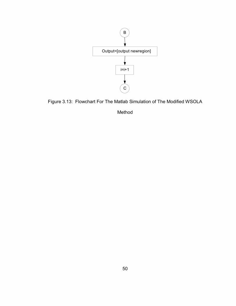
The modified WSOLA technique was simulated in Matlab. The flowchart

for the simulation is as presented in Figure 3.13.

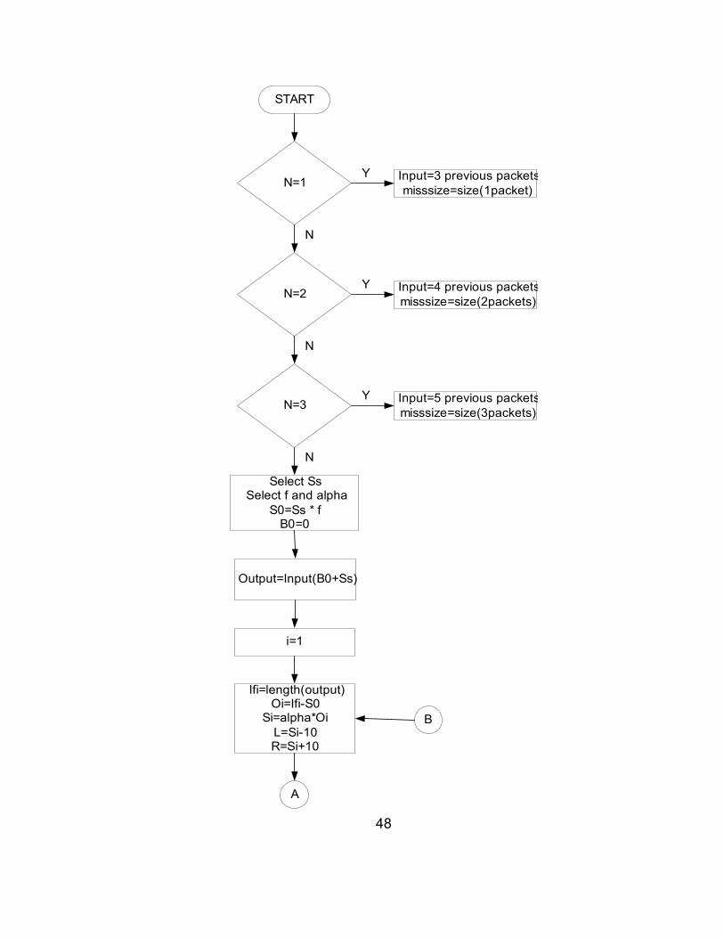
48

N=1

N=2

N=3

Input=3 previous packetsmisssize=size(1packet)

Input=4 previous packetsmisssize=size(2packets)

Input=5 previous packetsmisssize=size(3packets)

Y

Y

Y

N

N

N

Select SsSelect f and alpha

S0=Ss * fB0=0

START

Output=Input(B0+Ss)

i=1

Ifi=length(output)Oi=Ifi-S0

Si=alpha*OiL=Si-10R=Si+10

A

B

49

A

L<0 L=0Y

N

L=Si-10

Search region=Input(L:R)

Find Bi by performingnormalized cross correlation

on search region andOutput(Oi:Ifi)

R1=Input(Bi:Bi+S0) *Ramp1R2=(Oi:Ifi) *Ramp2

Overlapadd=R1+R2

Output=output[(1:Oi) overlapadd]

Length(output)>missize END

Newregion=(Bi+S0:Bi+So+So)

B

Y

N

50

Output=[output newregion]

B

C

i=i+1

Figure 3.13: Flowchart For The Matlab Simulation of The Modified WSOLA

Method

51

CHAPTER 4

RESULTS AND CONCLUSIONS

The pitch detection module and the modified WSOLA module work

together to form the entire packet loss reconstruction process. In this research

receiver based packet loss reconstruction was investigated. At the receiver, as

the first packet of the voice signal arrived it was stored in a buffer before it was

played out to the listener. The next five consecutive packets were also stored in

the buffer for a total of six packets. The six most recent packets were always

stored in the buffer at any given time. As the next packets arrived the most

recent packets were stored and the earlier packets erased. Packet loss

concealment was performed as follows:

1. The 3 most recently arrived packets concealed a lost packet.

2. The 4 most recently arrived packets concealed Consecutive lost

packets.

3. The 3 most recently arrived packets concealed consecutive packets.

If more than three consecutive packets were lost the quality of the recovered

speech was not good and the speech signal severely affected. In the case that

52

packets among the first six packets were lost, the preceding packets were used

for reconstruction.

At the receiver as the speech signal arrived it was first sampled at the rate of

20 KHz, then packetized to include 160 samples per packet and send through

the pitch detection module to calculate its pitch. The samples went through the

buffer where the six most recent samples were stored before they were played

out to the listener. Whenever the receiver detected lost packets the modified

WSOLA module activated to perform packet reconstruction and then the voice

signal was played out.

4.1 Measuring the Quality of Speech

In voice communications, the mean opinion score (MOS) provides a

numerical measure of the quality of human speech at the destination end of the

circuit. MOS is a widely accepted scheme used to test the quality of coders and

many other signal processing devices. The scheme uses subjective tests in the

form of opinionated scores that are mathematically averaged to obtain a

quantitative indicator of system performance. To determine MOS, a number of

listeners rate the quality of the speech spoken by male and female speakers. A

listener gives each sentence a rating from 1 to 5 where (1) is bad, (2) is poor, (3)

is fair, (4) is good and (5) is excellent. The MOS is the arithmetic mean of all the

individual scores and can range from 1, which is worst to 5, which is best.

53

4.2 Tests and Results

In order to test the new algorithm two tests were conducted. Eight voice

samples, four male and four female, with typical voice conversation were

recorded. Each sample had a length of 5 seconds. A sampling rate of 8 KHz

was used and the packet length was 160 samples per packet. Each speech

signal consisted of 250 packets, which were sampled at an 8 KHZ rate to yield

40,000 samples.

4.2.1 Test 1

Each of the eight voice samples was distorted in order to produce 1 lost

packet, 2 consecutive lost packets and 3 consecutive lost packets.

Reconstruction was performed using WSOLA and the modified WSOLA using

the following criteria:

1. The 3 most recently arrived packets concealed 1 lost packet.

2. The 4 most recently arrived packets concealed 2 consecutive lost

packets.

3. The 3 most recently arrived packets concealed 3 consecutive packets.

4.2.2 PESQ Score

PESQ stands for Perceptual Evaluation of Sound Quality and is an

enhanced perceptual quality measurement for voice quality in communication

networks. It was specifically developed to be applicable to end-to-end voice

54

quality testing under real network conditions. It is specified by the International

Telecommunications Union recommendation ITU-T P.861 [10]. This test rates

the quality of speech on a scale of 1 to 5. The worst score is 1 and the best

score is 5. The voice samples reconstructed by the modified WSOLA method

were subjected to the PESQ test.

A comparison of the PESQ test results for 1 random packet loss for the

WSOLA AND modified WSOLA methods are presented in Figure 4.1.

Figure 4.1: PESQ Scores For 1 Random Packet Loss

55

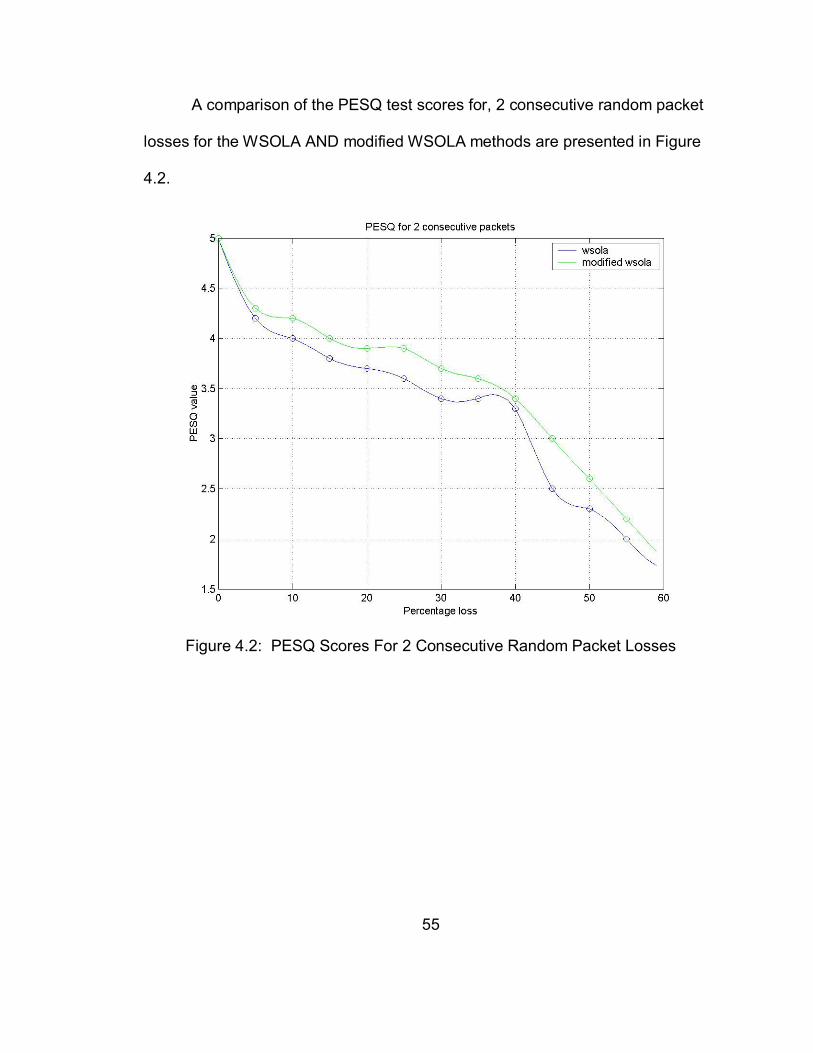
A comparison of the PESQ test scores for, 2 consecutive random packet

losses for the WSOLA AND modified WSOLA methods are presented in Figure

4.2.

Figure 4.2: PESQ Scores For 2 Consecutive Random Packet Losses

56

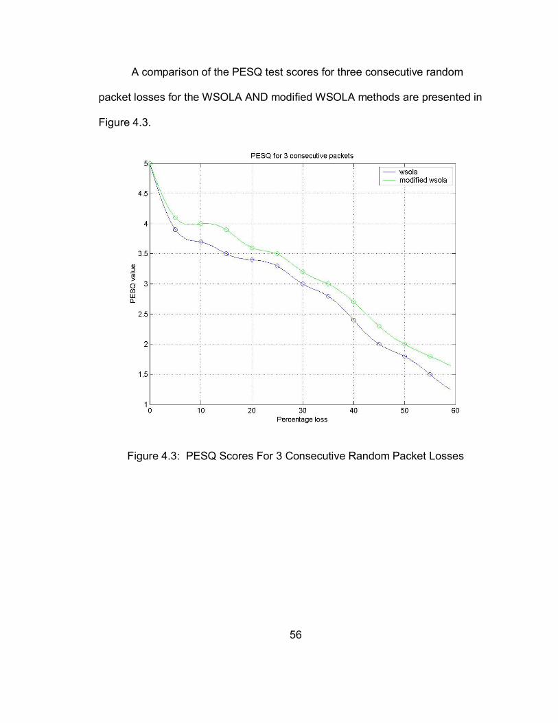
A comparison of the PESQ test scores for three consecutive random

packet losses for the WSOLA AND modified WSOLA methods are presented in

Figure 4.3.

Figure 4.3: PESQ Scores For 3 Consecutive Random Packet Losses

57

REFERENCES

[1] Werner Verhelst and Marc Roelands: “An overlap-add technique based on waveform similarity (WSOLA) for high quality time scale modification of speech”, 1993 IEEE International Conference on Acoustics, Speech, and Signal Processing, 1993. ICASSP-93., Volume: 2, 27-30 April 1993 Page(s): 554 -557 vol.2

[2] Alexander Stenger, Khaled Ben Younes, Bernd Girod: “A new error

concealment technique for audio transmission with packet loss”, Global Telecommunications Conference, 1996. GLOBECOM '96. 18-22 Nov.

1996, Page(s): 48 -52 [3] Yi Liang: “Loss Recovery and Adaptive Playout Control for Packet Voice

Communications over IP:, Presentation at Stanford University, April 19, 2000 http://ivms.stanford.edu/~liang/research/presentations/talk_2/talk2.pdf [4] S Yim, B Pawate: “Computationally efficient algorithms for time scale

modifications”, Conference Proceedings., 1996 IEEE International Conference on Acoustics, Speech, and Signal Processing, 1996. ICASSP-96. Volume: 2, 7-10 May 1996, Page(s): 1009 -1012 vol. 2

[5] Mei Yong: “Study of voice packet reconstruction methods applied to CELP

speech coding”, 1992 IEEE International Conference on Acoustics, Speech, and Signal Processing, 1992. ICASSP-92 Volume: 2, 23-26 March 1992, Page(s): 125 -128 vol.2

[6] Yi Liang, Bernd Girod: “Adaptive playout scheduling and loss concealment for

voice communication over Ip networks”, 2001 IEEE International Conference on Acoustics, Speech, and Signal Processing, 2001. Proceedings. (ICASSP '01). Volume: 3, 7-11 May 2001 Page(s): 1445 -1448 vol.3

[7] Luiz Dasilva, David Petr, Victor Frost: “A class oriented replacement

technique for lost speech packets”, INFOCOM '89. Proceedings of the Eighth Annual Joint Conference of the IEEE Computer and Communications Societies. Technology: Emerging or Converging? IEEE, 23-27 April 1989,

58

Page(s): 1098 -1105 vol.3 [8] Henning Sanneck: “Packet loss recovery and control for voice transmission over the internet”

[9] H. Sanneck: “Concealment of Lost Speech Packets Using Adaptive

Packetization”, IEEE International Conference on Multimedia Computing and Systems, 1998, 28 June-1 July 1998 Page(s): 140 -149

[10] Telecommunications Union recommendation ITU-T P.861, www.itu.org [11] Google search engine, www.google.com [12] Rafid A Sukkar, Joseph L LoCicero: “Design and Inplementation of a robust

pitch detector based on a parallel processing technique”, IEEE journal on selected areas in communication. Vol6, No2, February 1988

[13] Ejaz Mahfuz, “ Packet loss concealment for voice transmission over IP

networks” McGill University Canada, September 2001