Package ‘SARP.compo’ - cran.r-project.org · Package ‘SARP.compo’ May 21, 2018 Type Package Title Network-based Interpretation of Changes in Compositional Data Version 0.0.7

Package ‘SARP.compo’May 21, 2018

Type Package

Title Network-based Interpretation of Changes in Compositional Data

Version 0.0.7

Date 2018-05-10

Maintainer Emmanuel Curis <[email protected]>

License Artistic-2.0

Description Provides a set of functions to interpret changes incompositional data based on a network representation of all pairwise ratiocomparisons: computation of all pairwise ratio, construction of ap-value matrix of all pairwise tests of these ratios betweenconditions, conversion of this matrix to a network.

Suggests lme4

Depends igraph

Imports car

Encoding UTF-8

Language uk

NeedsCompilation no

Author Emmanuel Curis [aut, cre]

Repository CRAN

Date/Publication 2018-05-21 21:55:50 UTC

R topics documented:arbre.Mp . . . . . . . . . . . . . . . . . . . . . . . . . . . . . . . . . . . . . . . . . . . 2BpLi . . . . . . . . . . . . . . . . . . . . . . . . . . . . . . . . . . . . . . . . . . . . . 4calc.rapports . . . . . . . . . . . . . . . . . . . . . . . . . . . . . . . . . . . . . . . . . 5choisir.seuil . . . . . . . . . . . . . . . . . . . . . . . . . . . . . . . . . . . . . . . . . 6conversions . . . . . . . . . . . . . . . . . . . . . . . . . . . . . . . . . . . . . . . . . 8coupures.Mp . . . . . . . . . . . . . . . . . . . . . . . . . . . . . . . . . . . . . . . . 10creer_data.frame . . . . . . . . . . . . . . . . . . . . . . . . . . . . . . . . . . . . . . 12creer_graphe . . . . . . . . . . . . . . . . . . . . . . . . . . . . . . . . . . . . . . . . 14

1

2 arbre.Mp

creer_matrice . . . . . . . . . . . . . . . . . . . . . . . . . . . . . . . . . . . . . . . . 16modele . . . . . . . . . . . . . . . . . . . . . . . . . . . . . . . . . . . . . . . . . . . . 18poteries . . . . . . . . . . . . . . . . . . . . . . . . . . . . . . . . . . . . . . . . . . . 20puissance . . . . . . . . . . . . . . . . . . . . . . . . . . . . . . . . . . . . . . . . . . 21tests . . . . . . . . . . . . . . . . . . . . . . . . . . . . . . . . . . . . . . . . . . . . . 25

Index 28

arbre.Mp Grouping composants by changes in cut-off separation

Description

These functions construct a tree based on the successive disjunctions between nodes of the graphwhen increasing the cut-off value.

Usage

arbre.Mp( Mp, en.log = FALSE, reference = NA )

## S3 method for class 'Arbre'plot(x, seuil.p = 0.05,

xlab = "Composant",ylab = if ( TRUE == en.log ) "-log seuil" else "Seuil",col.seuil = "red" , lwd.seuil = 1, lty.seuil = 1,horiz = FALSE, center = TRUE, edge.root = TRUE,...)

Arguments

Mp A square, symmetric matrix containing p-values. Element in row i and line jshould contain the p-value for testing the i

j ratio. The diagonal is ignored.

en.log If TRUE, p-values are log-transformed (using decimal logarithm) to construct thetree. It does not change the tree structure, it only helps visualisation of the smallp-value part of the tree.

reference Either NA (the default) or a vector giving the names of reference genes. Cor-responding leaves will then be drawn in orange, whereas leaves for genes ofinterests will be drawn in palegreen (like graphs).

x The tree to be drawn

seuil.p Selected cut-off for analysis. Can also be a SARPcompo.H0 object, as returnedby choisir.seuil, in which case the bounds of the confidence interval are alsodrawn, with dashed lines by default.

xlab,ylab Legends for the axescol.seuil, lwd.seuil, lty.seuil

Graphical parameters for drawing the analysis cut-off

arbre.Mp 3

horiz, center, edge.root

Options from plot.dendrogram with different defaults or needed for comple-mentary plottings. If TRUE, the tree is drawn, respectivally, horizontally insteadof vertically, with edges “centered”, and with edge to the root node. See thedocumentation from plot.dendrogram for details.

... Additionnal parameters for plot.dendrogram, which is used internally.

Details

By increasing the cut-off from 0 to 1, more and more edges between nodes are removed, anddisjoint subgraphs appear. This can be used to build a tree of the composants, with nodes of thetree corresponding to the apparition of a new distinct subgraph. Leafs of the tree are the individualcomponents.

Value

The arbre.Mp function returns a dendrogram.

Author(s)

Emmanuel Curis (<[email protected]>)

See Also

creer.Mp to create a matrix of p-values for all possible ratios of a compositional vector.

grf.Mp to convert such a matrix to a graph, once a cut-off is selected.

coupures.Mp to obtain the set of p-values corresponding to the nodes of the tree, that is to theapparition of new sets of composants.

plot.dendrogram and as.dendrogram for more details on dendrogram drawing and structure.

Examples

# load the potery data setdata( poteries )

# Compute one-way ANOVA p-values for all ratios in this data setMp <- creer.Mp( poteries, c( 'Al', 'Na', 'Fe', 'Ca', 'Mg' ),

f.p = anva1.fpc, v.X = 'Site' )

# Build the tree (in log scale, p-values are all < 0.01)arbre <- arbre.Mp( Mp, en.log = TRUE )

# It is a dendrogram as defined in the cluster packagestr( arbre )class( arbre )

# Drawing this treeplot( arbre )

4 BpLi

BpLi Circadian Genes Expression in Bipolar Disorder Patients

Description

These two datasets give the expression level of main circadian genes in lymphoblastoid cells frombipolar disorder patients, as determined by qRT-PCR. Results are expressed in cycle thresholds(CT) units.

Usage

data(BpLi_J2)data(BpLi_J4)

Format

Each dataset is a data frame with 78 rows and 26 columns. Each row give the RNA quantificationof circadian and control genes for lymphoblastoid cells of a given patient, either with or withoutlithium in the culture medium.

Phenotype factor Patient phenotype, either responding (R) or not (NR) to lithiumPatient integer Patient code

Li factor Is lithium present (Oui) or not (Non) in the culture medium of the cells

Other columns are the different circadian genes and reference genes expression levels, expressedas quantities in arbitrary units after quantitative reverse transcription PCR assays, using the SyberGreen technology. Three sets of assays were done, using three different dilutions according tothe explored gene: 1/20 (PER3, BHLHE41, NR1D1, DBP), 1/100 (GSK3b, RORA, PER1, PER2,CLOCK, ARNTL, CRY2, BHLHE40) and 1/200 (ARNTL2, TIMELESS, CRY1, CSNK1E). Thenumerical suffixe after the reference gene name (SDHA or HPRT) gives this dilution level – forinstance, SDHA_20 is for the 1/20 dilution level, HRPT_100 for the 1/100 level...

Patients were classified as presenting a good response (R) or a lack of responce (NR) to lithiumtreatment based on the ALDA scale, see the original publication for details. Lymphoblastoid cellsfrom each patients, obtained from blood samples, were cultivated for 2 (BpLi_J2) or 4 (BpLi_J4)days either with or without LiCl.

Source

Data courtesy allowed to be included in the package, by Cynthia Marie-Claire.

References

Geoffrey, P. A., Curis E., Courtin, C., Moreira, J., Morvillers, T., Etain, B., Laplanche, J.-L., Bel-livier, F. and Marie-Claire, C. (2017). Lithium response in bipolar disorders and core clock genesexpression. World J Biol Psychiatry, doi: 10.1080/15622975.2017.1282174.

calc.rapports 5

calc.rapports Compute all pairwise ratios of a set of variables

Description

This function computes all pairwise ratios or differences of a set of variables in a given data frame

Usage

calc.rapports( d, noms, log = FALSE, isoler = FALSE )

Arguments

d The data frame that contains the variables. Other objects will be coerced as dataframes using as.data.frame

noms A character vector containing the column names of the compositional variablesto be used for ratio computations. Names absent from the data frame will beignored with a warning.Optionnally, an integer vector containing the column numbers can be given in-stead. They will be converted to column names before further processing.

log If TRUE, values in the columns are assumed to be log-transformed, and conse-quently ratios are computed as differences of the columns. The result is in thelog scale.If FALSE, values are assumed to be raw data and ratios are computed directly.

isoler If TRUE, the result data frame will not include the original values.

Details

Use this function to compute all pairwise ratio of a set of numerical variables. If non-numericalvariables are given in the list of variables, they will be ignores with a warning.

Since the ratio of variables i and j is the inverse of the ratio of variables j and i, only one of them iscomputed. The order is determined by the order of the variables in noms. In matrix notations, onlythe upper right matrix is computed, withour the diagonal.

Value

These function returns the original data.frame with additional columns corresponding to all pairwiseratios added as the last columns of the data.frame.

These variables have their name constructed as the concatenation of the names of the two variablesused, the first one being at the numerator, separated with a dot and with the additional suffix .r (or.r.log is working on difference of logarithms).

Their order is determined by the order given in noms: the first variable of the list, V1, is used tocompute ratios with all others (V1/V2, V1/V3 and so on). Then the second one is used for ratiosfurther ones (V2/V3 and so on), and so on until the last one.

6 choisir.seuil

Note

This function is mainly for designing a step-by-step analysis or control purposes. To avoid waste ofmemory, most of the functions in the package actually compute “on fly” the ratios when constructingthe matrix or the data frame of p-values.

Author(s)


See Also

creer.Mp to create a matrix of p-values for all pairwise tests of ratio changes.

Examples


# Compute all ratios in the potery data setd.r <- calc.rapports( d = poteries, noms = c( 'Al', 'Fe', 'Mg', 'Ca','Na' ) )names( d.r )head( d.r )

identical( d.r$Al.Fe.r, d.r$Al / d.r$Fe )

choisir.seuil Cut-off selection by simulations

Description

Obtaining the optimal p-value cut-off for individual tests to achieve a given Type I error level ofobtaining disjoint components of the graph

Usage

choisir.seuil( n.genes,taille.groupes = c( 10, 10 ),alpha.cible = 0.05,seuil.p = (5:30)/100,B = 3000, conf.level = 0.95,f.p = student.fpc, frm = R ~ Groupe,normaliser = FALSE, en.log = TRUE,n.quantifies = n.genes,masque, ... )

choisir.seuil 7

Arguments

n.genes Number of genes to be quantified simultaneously

taille.groupes An integer vector containing the sample size for each group. The number ofgroups is determined by the length of this vector. Unused if masque is provided.

alpha.cible The target type I error level of obtaining disjoint subnetworks under the nullhypothesis that gene expressions are the same in all groups. Should be between0 and 1.

seuil.p A numeric vector of candidate cutoffs. Values outside the [0,1] interval areautomatically removed. The default (from 0.05 to 0.30) is suited for a targettype I error of 0.05 and less than 30 genes, roughly.

B How many simulations to do.

conf.level The confidence level of the interval given as a result (see Details).

f.p The function to use for individual tests of each ratio. See creer.Mp for details.

frm The formula to use. The default is suited for the structure of the simulated data,with R the ratio and Groupe the variable with group membership.

normaliser Should the simulated data by normalised, that is should their sum be equal to1? Since ratio are insensitive to the normalisation (by contrast with individualquantities), it is a useless step for usual designs, hence the default.

en.log If TRUE, generated data are seen as log of quantities, hence the normalisationstep is performed after exponentiation of the data and data are converted back inlog.The option is also used in the call of creer.Mp.

n.quantifies The number of quantified genes amongst the n.genes simulated. Must be atmost equal to n.genes, which is the default.

masque A data.frame containing the values of needed covariates for all replicates. Ifmissing, a one-column data.frame generated using taille.groupes, the col-umn (named ‘Groupe’) containing values ‘G1’ repeated taille.groupes[ 1 ]times, ‘G2’ repeated taille.groupes[ 2 ] times and so on.

... additional arguments, to be used by the analysis function f.p

Details

The choisir.seuil function simulates B datasets of n.genes “quantities” measured several times,under the null hypothesis that there is only random variations between samples. For each of these Bdatasets, creer.Mp is called with the provided test function, then converted to a graph using in turnall cut-offs given in seuil.p and the number of components of the graph is determined. Havingmore than one is a type I error.

For each cut-off in seuil.p, the proportion of false-positive is then determined, along with itsconfidence interval (using the exact, binomial formula). The optimal cut-off to achieve the targettype I error is then found by linear interpolation.

Simulation is done assuming a log-normal distribution, with a reduced, centered Gaussian on thelog scale. Since under the null hypothesis nothing changes between the groups, the only neededinformations is the total number of values for a given gene, which is determined from the numberof rows of masque. All columns of masque are transfered to the analysis function, so simulation

8 conversions

under virtually any experimental design should be possible, as far as a complete null hypothesis iswanted (not any effect of any covariate).

Value

choisir.seuil returns a data.frame with four columns, corresponding to the candidate cut-offs,the corresponding estimated type-I error and its lower and upper confidence bounds, and attributesgiving the estimated optimal cut-off, its confidence interval and details on simulation condition.This data.frame has the additional class SARPcompo.H0, allowing specific print and plot methodsto be used.

Warning

The simulated ratios are stored in a column called R, appended to the simulated data.frame. For thisreason, do not use any column of this name in the provided masque: it would be overwritten duringthe simulation process.

Author(s)


See Also

creer.Mp.

Examples

# What would be the optimal cut-off for 10 genes quantified in two# groups of 5 replicates?# For speed reason, only 50 simulations are done here,# but obviously much more are needed to have a good estimate f the cut-off.

seuil <- choisir.seuil( 10, c( 5, 5 ), B = 50 )seuil

# Get the cut-off and its confidence intervalattr( seuil, "seuil" )

# Plot the resultsplot( seuil )

conversions Convert between matrix and data-frame format

Description

These functions convert all pairwise ratio tests between the matrix format and the data.frame format

conversions 9

Usage

Mp.DFp(DFp, col.noms = c( 1, 2 ), col.p = 'p')

Arguments

DFp Results in the data.frame format.

col.noms A length two character vector giving the columns in the data.frame format thatcontain the names of the two components of which the ratio is tested. If con-verting from a data.frame, can be given by number.

col.p A length one character vector giving the column containing the p-values of thetest in the data.frame format. If converting from a data.frame, can be given bynumber.

Details

The matrix format is more convenient for manipulations like finding cut-off probabilities or buildingthe hierarchical tree of the components. However, it can only store one value per couple and is morememory consuming.

The data.frame format is more efficient for computations, since it allows to store several resultsat once. It can also be easily saved and read using text-files and read.table or write.table.However, finding the hierarchical tree of components or building the graph is not so straightforward.

These utilitary functions allow to convert between the two formats.

Value

The results in the other format: a matrix for Mp.DFp and a 3-columns data.frame for DFp.Mp.

In the matrix form, components will be sorted by alphabetical order.

Warning

When converting a data.frame to a matrix, there is no control that all possible combinations arepresent once, and only once, in the data.frame. Missing combinations will have 0 in the matrix;combinations present several time will have the value of the last replicate.

When converting a matrix to a data.frame, the diagonal is not included in the data.frame. The matrixis expected to be symmetric, and only the upper right part is used.

Author(s)


See Also


creer.DFp to create a data.frame of p-values for all possible ratios of a compositional vector.

10 coupures.Mp

Examples

# load the potery data set data( poteries )

coupures.Mp Finding cut-offs for graph disjonctions

Description

These functions detect the experimental cut-offs to create distinct subgraphs, and propose adaptedgraphical representation.

Usage

coupures.Mp( Mp )

## S3 method for class 'Coupures'plot(x, seuil.p = 0.05, en.log = TRUE,

xlab = "Seuil de p", ylab = "Nombre de composantes",col.trait = "black", lwd.trait = 1, lty.trait = 1,col.seuil = "red" , lwd.seuil = 1, lty.seuil = 1,pch.fin = 19, cex.fin = 1, col.fin ="darkgreen",pch.deb = ")", cex.deb = 1, col.deb = "darkgreen",...)

Arguments



x The set of critical values, as obtained by coupures.Mp

seuil.p Selected cut-off for analysis. Can also be a SARPcompo.H0 object, as returnedby choisir.seuil, in which case the bounds of the confidence interval are alsodrawn, with dashed lines by default.

en.log If TRUE, the p-values axis uses a decimal logarithm scale. It may help visualisa-tion of the small critical p-values.

xlab,ylab Legends for the axescol.trait, lwd.trait, lty.trait, pch.fin, cex.fin, col.fin, pch.deb, cex.deb, col.deb

Graphical parameters for drawing the number of components in function of thecut-off. ‘trait’ refers to the function itself, ‘deb’ to the first point of a region ofconstant components number (that does not belong to it: the function is right-discontinuous) and ‘fin’ to the last point of this region (that belongs to it)

col.seuil, lwd.seuil, lty.seuil

Graphical parameters for drawing the analysis cut-off

... Additionnal parameters for plot, which is used internally.

coupures.Mp 11

Details

By increasing the cut-off from 0 to 1, more and more edges between nodes are removed, and disjointsubgraphs appear. This function detects in a matrix of p-values which are the “critical” ones, that isthe one for which the number of components changes.

Because the edge removal is defined by p < cut− off , the cut-off returned for a given number ofcomponents is to be understand as the maximal one that gives this number of components.

The plot method allows to visualize the evolution of the number of components with the cut-off,and writes the critical cut-off values.

Value

The coupures.Mp function returns a data.frame with additionnal class ‘Coupures’. It contains threecolumns: one with the p-value cut-offs, one with the opposite of their decimal logarithm and onewith the number of components when using exactly this cut-off. The additionnal class allows toprovide a plot method.

Author(s)


See Also


grf.Mp to convert such a matrix to a graph, once a cut-off is selected.

arbre.Mp to convert such a matrix to a classification tree of the components of the compositionalvector.

Examples



f.p = anva1.fpc, v.X = 'Site' )

# Where would be the cut-offs?seuils <- coupures.Mp( Mp )seuils

# Drawing this, in log10 scaleplot( seuils, en.log = TRUE )

12 creer_data.frame

creer_data.frame Create p-values data-frame from pairwise tests of all possible ratiosof a compositional vector

Description

This function performs hypothesis testing on all possible pairwise ratios or differences of a set ofvariables in a given data frame, and store their results in a data.frame

Usage

creer.DFp( d, noms, f.p = student.fpc,log = FALSE, en.log = !log,nom.var = 'R',noms.colonnes = c( "Cmp.1", "Cmp.2", "p" ),add.col = "delta",... )

Arguments

d The data frame that contains the compositional variables. Other objects will becoerced as data frames using as.data.frame


f.p An R function that will perform the hypothesis test on a single ratio (or log ratio,depending on log and en.log values).This function should return a numeric vector, of which the first one will typicallybe the p-value from the test — see creer.Mp for details.Such functions are provided for several common situations, see references at theend of this manual page.


en.log If TRUE, the ratio will be log-transformed before applying the hypothesis testcomputed by f.p. Don’t change the default unless you really know what youare doing.

nom.var A length-one character vector giving the name of the variable containing a singleratio (or log-ratio). No sanity check is performed on it: if you experience strangebehaviour, check you gave a valid column name, for instance using make.names.

creer_data.frame 13

noms.colonnes A length-three character vector giving the names of, respectively, the two columnsof the data frame that will contain the components identifiers and of the columnthat will contain the p-value from the test (the first value returned by f.p).

add.col A character vector giving the names of additional columns of the data.frame,used for storing additional return values of f.p (all but the first one).

... additional arguments to f.p, passed unchanged to it.

Details

This function constructs a data.frame with n× (n− 1)/2 rows, where n = length( noms ) (aftereventually removing names in noms that do not correspond to numeric variables). Each line of thedata.frame is the result of the f.p function when applied on the ratio of variables whose names aregiven in the first two columns (or on its log, if either (log == TRUE) && (en.log == FALSE)or (log == FALSE) && (en.log == TRUE)).

Value

These function returns the data.frame obtained as described above.

Note

Creating a data.frame seems slightly less efficient (in terms of speed) than creating a dense matrix,so for compositionnal data with only a few components and simple stastitical analysis were only asingle p-value is needed, consider using creer.Mp instead.

Author(s)


See Also

Predefined f.p functions: anva1.fpc for one-way analysis of variance; kw.fpc for the non-parametricequivalent (Kruskal-Wallis test).

grf.DFp to create a graphe from the obtained matrix.

Examples

# load the Circadian Genes Expression dataset, at day 4data( "BpLi_J4" )ng <- names( BpLi_J4 )[ -c( 1:3 ) ] # Name of the genes

# analysis function (complex design)# 1. the formula to be usedfrm <- R ~ (1 | Patient) + Phenotype + Li + Phenotype:Li

# 2. the function itself# needs the lme4 packageif ( TRUE == require( "lme4" ) ) {

f.p <- function( d, variable, ... ) {# Fit the model

14 creer_graphe

md <- lmer( frm, data = d )

# Get coefficients and standard errorscf <- fixef( md )se <- sqrt( diag( vcov( md ) ) )

# Wald tests on these coefficientsp <- 2 * pnorm( -abs( cf ) / se )

# Sending back the 4 p-valuesp

}

# CRAN does not like 'long' computations# => analyse only the first 6 genes# (remove for real exemple!)ng <- ng[ 1:6 ]

# Create the data.frame with all resultsDF.p <- creer.DFp( d = BpLi_J4, noms = ng,

f.p = f.p, add.col = c( 'p.NR', 'p.Li', 'p.I' ) )

# Make a graphe from it and plot it# for the interaction term, at the p = 0.2 thresholdplot( grf.DFp( DF.p, p = 0.20, col.p = 'p.I' ) )

}

creer_graphe Create a graph using a set of p-values from pairwise tests

Description

These functions construct an undirected graph, using the igraph package, to represent and investi-gate the results of all testing of all ratios of components of a compositional vector.

Usage

grf.Mp( Mp, p = 0.05, reference = NULL, groupes = NULL )

grf.DFp( DFp, col.noms = c( 1, 2 ), p = 0.05, col.p = 'p',reference = NULL, groupes = NULL )

Arguments



DFp A data frame containing at least three columns: two with component names andone with p-values for the corresponding ratio.

creer_graphe 15

col.noms A length two vector giving the names of the two columns containing the com-ponents names.

p The p-value cutoff for adding an edge between two nodes. See details.

col.p The name of the column containing the p-values to use to create the graph.

reference A character vector giving the names of nodes that should be displayed with adifferent color in the created graph. These names should match column namesused in Mp. Typical use would be for reference genes in qRT-PCR experiments.By default, all nodes are displayed in palegreen; reference nodes, if any, will bedisplayed in orange.

groupes

Details

Consider a compositional vector of n components. These n are seen as the nodes of a graph. Nodesi and j will be connected if and only if the p-value for the test of the i

j ratio is higher than the cutoff,p – that is, if the test is not significant at the level p.

Strongly connected sets of nodes will represent components that share a similar behaviour betweenthe conditions tested, whereas unrelated sets of nodes will have a different behaviour.

Value

These function returns the created graph. It is an igraph object on which any igraph function can beapplied, including plotting, and searching for graph components, cliques or communities.

Author(s)


See Also


creer.DFp to create a data.frame of p-values for all possible ratios of a compositional vector.

Examples



f.p = anva1.fpc, v.X = 'Site' )Mp

# Make a graphe from it and plot itplot( grf.Mp( Mp ) )

16 creer_matrice

creer_matrice Create p-values matrix from pairwise tests of all possible ratios of acompositional vector

Description

This function performs hypothesis testing on all possible pairwise ratios or differences of a set ofvariables in a given data frame, and store their results in a (symmetric) matrix

Usage

creer.Mp( d, noms, f.p, log = FALSE, en.log = !log,nom.var = 'R', ... )

Arguments

d The data frame that contains the compositional variables. Other objects will becoerced as data frames using as.data.frame


f.p An R function that will perform the hypothesis test on a single ratio (or log ratio,depending on log and en.log values).This function should return a single numerical value, typically the p-value fromthe test.This function must accept at least two named arguments: d that will contain thedata frame containing all required variables and variable that will contain thename of the column that contains the (log) ratio in this data frame. All otherneeded arguments can be passed through ....Such functions are provided for several common situations, see references at theend of this manual page.


en.log If TRUE, the ratio will be log-transformed before applying the hypothesis testcomputed by f.p. Don’t change the default unless you really know what youare doing.

nom.var A length-one character vector giving the name of the variable containing a singleratio (or log-ratio). No sanity check is performed on it: if you experience strangebehaviour, check you gave a valid column name, for instance using make.names.

... additional arguments to f.p, passed unchanged to it.

creer_matrice 17

Details

This function constructs a n×n matrix, where n = length( noms ) (after eventually removingnames in noms that do not correspond to numeric variables). Term (i, j) in this matrix is the resultof the f.p function when applied on the ratio of variables noms[ i ] and noms[ j ] (or on its log,if either (log == TRUE) && (en.log == FALSE) or (log == FALSE) && (en.log == TRUE)).

The f.p function is always called only once, for i < j, and the other term is obtained by symmetry.

The diagonal of the matrix is filled with 1 without calling f.p, since corresponding ratios are alwaysidentically equal to 1 so nothing useful can be tested on.

Value

These function returns the matrix obtained as described above, with row an column names set tothe names in noms (after conversion into column names and removing all non-numeric variables).

Note

Since the whole matrix is stored and since it is a dense matrix, memory consumption (and com-putation time) increases as n2. For compositional data with a large number of components, like inRNA-Seq data, consider instead creating a file.

Author(s)


See Also

Predefined f.p functions: anva1.fpc for one-way analysis of variance; kw.fpc for the non-parametricequivalent (Kruskal-Wallis test).

grf.Mp to create a graphe from the obtained matrix.

Examples



f.p = anva1.fpc, v.X = 'Site' )Mp


18 modele

modele Create a compositional model for simulations

Description

These functions create and plot a model of compositionnal data for two or more conditions.

Usage

modele_compo( medianes, en.log = FALSE,noms = colnames( medianes ),conditions = rownames( medianes ),reference = NULL, total = 1 )

## S3 method for class 'SARPcompo.modele'plot( x,

xlab = "Composant",ylab.absolu = "Quantit\u00e9", ylab.relatif = "Fraction",taille.noeud = 50, ... )

Arguments

medianes A matrix giving the medians of all components quantities in each condition.Each row of this matrix corresponds to a different condition; each column, toone of the components.

en.log If TRUE, the values in the matrix are given in the log scale.

noms Names of the components. If provided, should be a character vector whoselength is equal to the number of columns of medianes.

conditions Names of the different conditions. If provided, should be a character vectorwhose length is equal to the number of rows of medianes.

reference A character vector giving the names of the components used as reference (typi-cally, reference genes in qRT-PCR).

total The total amount. The sum of amounts in each condition will equal this total,when the data are made compositionnal.Arguments for the plot method

x The modele to be plotted

xlab Legend for the X axis

ylab.absolu Legend for the Y axis, in the amount scale (no constrain)

ylab.relatif Legend for the Y axis, in the compositional scale.

taille.noeud The plot size of nodes of the theoretical graph

... Additionnal parameters for plot, which is used internally.

modele 19

Details

The modele_compo function creates a compositionnal data model using the quantites provided: itconverts amounts in fractions of the total amount for each condition, then computes the theoreticalgraph showing classes of equivalents components, that is components that have the same evolutionbetween the two conditions. If more than two conditions are given, graphs correspond to compari-son of each condition with the first one.

The plot methods represents the original quantities, the quantities after conversion in compositionaldata ant the theoretical graph.

Value

An object of class SARPcompo.modele, with a plot method. It is a list with the following elements:

Absolue The matrix of quantities in amount scale

Relative The matrix of quantities in compositional data scale

Graphes A list of length nrow(medianes) - 1. Each element of the list gives, forthe corresponding condition, the matrix of all ratios of pairwise ratios betweencondition and the first condition (element M.rapports), the corresponding con-nectivity matrix (element M.connexion), the graph of component changes com-pared to the first condition (element Graphe, an igraph object) and the list ofcomponents of this graph (element Connexe, obtained from the componentsfunction.

It also stores a few informations as attributes.

Author(s)


See Also

estimer.puissance and estimer.alpha to use these models in simulations to study power andtype I error of the method in a given situation.

Examples

## Create a toy example: four components, two conditions## components 1 and 2 do not change between conditions## component 3 is doubled## component 4 is halfedme <- rbind( 'A' = c( 1, 1, 1, 1 ),

'B' = c( 1, 1, 2, 0.5 ) )colnames( me ) <- paste0( "C-", 1:4 )

md <- modele_compo( me )

## Plot it...plot( md )

20 poteries

## What is approximately the power to detect that something changes## between conditions A and B using a Student test## with a CV of around 50 % ?## (only a few simulations for speed, should be increased )puissance <- estimer.puissance( md, cv = 0.50, B = 50, f.p = student.fpc )plot( puissance )

poteries Composition of Roman poteries

Description

This data set gives the oxide composition of several potteries found in five different archaelogicsites of the United Kingdom. Composition was obtained using atomic absorption spectrometry.

Usage

data(poteries)

Format

A data frame with 14 columns and 48 rows. Each row gives the composition of a pottery (columns2 to 10), the archaelogical site where it was found (columns 6 and 7):

ID factor Pottery sample identifier (see original paper appendix)Al numeric Percentage of aluminium oxideFe numeric Percentage of iron oxide

Mg numeric Percentage of magnesium oxideCa numeric Percentage of calcium oxideNa numeric Percentage of natrium oxideK numeric Percentage of kalium oxideTi numeric Percentage of titanim oxide

Mn numeric Percentage of manganese oxideBa numeric Percentage of baryum oxide

Site factor Kiln sitePays factor Location of the kiln site

Couleur factor External color of the potteryDate factor Approximate date of the pottery

Note

The DASL version of the dataset, as presented in the "Pottery stoty", does not include data on thepoteries from the Gloucester site, neither the data on K, Ti, Mn and Ba oxides. It neither includesthe color and date informations, and codes sites as their first letter only.

The DASL version of the dataset exists in the car package, as the Pottery dataset (with twolocations differently spelled).

puissance 21

Source

Downloaded from the DASL (Data and Story Library) website, and completed from the originalpaper of Tubb et al.

References

A. Tubb, A. J. Parker, and G. Nickless (1980). The analysis of Romano-British pottery by atomicabsorption spectrophotometry. Archaeometry, 22, 153-171.

Hand, D. J., Daly, F., Lunn, A. D., McConway, K. J., and E., O. (1994) A Handbook of Small DataSets. Chapman and Hall – for the short version of the dataset.

Examples

data( poteries )# Reconstruct the car version of this datasetdcar <- poteries[ , c( 'Al', 'Fe', 'Mg', 'Ca', 'Na', 'Site' ) ]dcar <- droplevels( dcar[ -which( dcar$Site == "College of Art" ), c( 6, 1:5 ) ] )levels( dcar$Site )[ c( 1, 3, 4 ) ] <- c( "AshleyRails", "Islethorns", "Llanedyrn" )

# Reconstruct the DASL version of this datasetdasl <- dcar[ , c( 2:6, 1 ) ]levels( dasl$Site ) <- c( 'A', 'C', 'I', 'L' )

puissance Estimate the power and the type-I error of the disjoint-subgraphsmethod

Description

Estimate the power and the type-I error of the disjoint-graph method to detect a change in compo-sitions between different conditions

Usage

estimer.puissance( composition, cv.composition,taille.groupes = 10, masque,f.p, v.X = 'Condition',seuil.candidats = ( 5:30 ) / 100,f.correct = groupes.identiques,groupes.attendus = composition$Graphes[[ 1 ]]$Connexe,

avec.classique = length( attr( composition, "reference" ) ) > 0,f.correct.classique = genes.trouves,genes.attendus,B = 3000,... )

estimer.alpha( composition, cv.composition,

22 puissance

taille.groupes = 10, masque,f.p, v.X = 'Condition',seuil.candidats = ( 5:30 ) / 100,avec.classique = length( attr( composition, "reference" ) ) > 0,B = 3000,... )

Arguments

composition A composition model, as obtained by modele_compo. For simulations under thenull hypothesis (estimer.alpha), the first condition is duplicated to other con-ditions (but not the cv.composition, if provided as a matrix, allowing to exploresome kinds of pseudo-null hypothesis).

cv.composition The expected coefficient of variation of the quantified amounts. Should be eithera single value, that will be used for all components and all conditions, or amatrix with the same structure than composition$Absolue: one row for eachcondition, one column for each component, in the same order and with the samenames. Coefficients of variations are expected in the amount scale, in raw form(that is, give 0.2 for a 20% coefficient of variation).

taille.groupes The sample size for each condition. Unused if masque is given. If a single value,it will be used for all conditions. Otherwise, should have the same length thatthe number of conditions in the provided model.

masque A data.frame that will give the dataset design for a given experiment. Shouldcontain at least one column containing the names of the conditions, with valuesbeing in the conditions names in composition. If not provided, it is generatedfrom taille.groupes as a single column named ‘Condition’.

f.p The function used to analyse the dataset. See creer.Mp for details.v.X The name of the column identifying the different conditions in masque.seuil.candidats

A vector of p-value cut-offs to be tested. All values should be between 0 and 1.f.correct A function to determine if the result of the analysis is the expected one. Defaults

to a function that compares the disjoint sub-graphs of a reference graph and theobtained one.

groupes.attendus

The reference graph for the above function. Defaults to the theoretical graph ofthe model, for the comparison between the first and the second conditions.

avec.classique If TRUE, analysis is also done using an additive log-ratio (alr)-like method, usingthe geometric mean of the reference components as the “normalisation factor”.This correspond to the Delta-Delta-Ct method, or similar methods, in qRT-PCR.With this method, each non-reference component is tested in turn after divisionby the normalisation factor.If requested, the analysis is done with and without multiple testing correction(with Holm’s method). The “cut-off p-value” is used as the nominal type~Ierror level for the individual tests.

f.correct.classique

A function to determine if the alr-like method finds the correct answer. Defaultsto a function that compares the set of significant tests with the set of expectedcomponents.

puissance 23

genes.attendus A character vector giving the names of components expected to behave differ-ently than the reference set.

B The number of simulations to be done.

... Additionnal parameters for helper functions, including f.p, f.correct andf.correct.classique

Details

Use this function to simulate experiments and explore the properties of the disjoint graph methodin a specified experimental context. Simulations are done using a log-normal model, so analysis isalways done on the log scale. Coefficients of variation in the original scale hence directly translateinto standard deviations in the log-scale.

For power analysis, care should be taken that any rejection of the null hypothesis “nothing is dif-ferent between conditions” is counted as a success, even if the result does not respect the originalchanges. This is the reason for the additional correct-finding probability estimation. However,defining what is a correct, or at least acceptable, result may be not straightforward, especially forcomparison with other analysis methods.

Note also that fair power comparisons can be done only for the same type I error level. Hence, forinstance, power of the corrected alr-like method at p = 0.05 should be compared to the power of thedisjoint-graph method at its “optimal” cut-off.

Value

An object of class SARPcompo.simulation, with a plot method. It is a data.frame with the followingcolumns:

Seuil The cut-offs used to build the graph

Disjoint The number of simulations that led to disjoint graphs.

Correct The number of simulations that led to the correct graph (as defined by thef.correct function).

If avec.classique is TRUE, it has additionnal columns:

DDCt The number of simulations that led at least one significant test using the alr-likemethod.

DDCt.H The number of simulations that led at least one significant test using the alr-likemethod, after multiple testing correction using Holm’s method.

DDCt.correct The number of simulations that detected the correct components (as defined bythe f.correct.classique function) using the alr-like method.

DDCt.H.correct As above, but after multiple testing correction using Holm’s method.

It also stores a few informations as attributes, including the total number of simulations (attributen.simulations).

Author(s)


24 puissance

See Also

modele_compo to create a compositional model for two or more conditions.

creer.Mp, which is used internally, for details about analysis functions.

choisir.seuil for a simpler interface to estimate the optimal cut-off.

Examples

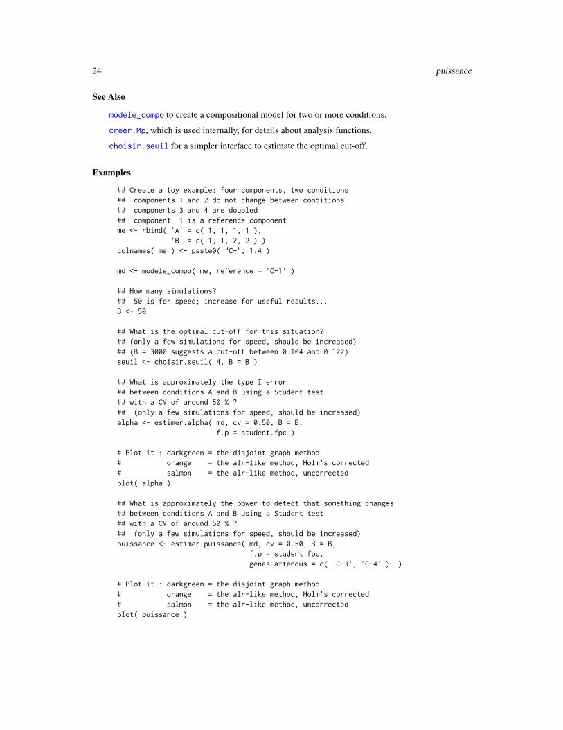
## Create a toy example: four components, two conditions## components 1 and 2 do not change between conditions## components 3 and 4 are doubled## component 1 is a reference componentme <- rbind( 'A' = c( 1, 1, 1, 1 ),

'B' = c( 1, 1, 2, 2 ) )colnames( me ) <- paste0( "C-", 1:4 )

md <- modele_compo( me, reference = 'C-1' )

## How many simulations?## 50 is for speed; increase for useful results...B <- 50

## What is the optimal cut-off for this situation?## (only a few simulations for speed, should be increased)## (B = 3000 suggests a cut-off between 0.104 and 0.122)seuil <- choisir.seuil( 4, B = B )

## What is approximately the type I error## between conditions A and B using a Student test## with a CV of around 50 % ?## (only a few simulations for speed, should be increased)alpha <- estimer.alpha( md, cv = 0.50, B = B,

f.p = student.fpc )

# Plot it : darkgreen = the disjoint graph method# orange = the alr-like method, Holm's corrected# salmon = the alr-like method, uncorrectedplot( alpha )

## What is approximately the power to detect that something changes## between conditions A and B using a Student test## with a CV of around 50 % ?## (only a few simulations for speed, should be increased)puissance <- estimer.puissance( md, cv = 0.50, B = B,

f.p = student.fpc,genes.attendus = c( 'C-3', 'C-4' ) )

# Plot it : darkgreen = the disjoint graph method# orange = the alr-like method, Holm's corrected# salmon = the alr-like method, uncorrectedplot( puissance )

tests 25

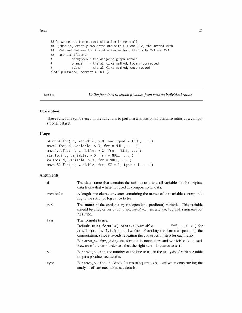
## Do we detect the correct situation in general?## (that is, exactly two sets: one with C-1 and C-2, the second with## C-3 and C-4 --- for the alr-like method, that only C-3 and C-4## are significant)# darkgreen = the disjoint graph method# orange = the alr-like method, Holm's corrected# salmon = the alr-like method, uncorrectedplot( puissance, correct = TRUE )

tests Utility functions to obtain p-values from tests on individual ratios

Description

These functions can be used in the functions to perform analysis on all pairwise ratios of a compo-sitional dataset

Usage

student.fpc( d, variable, v.X, var.equal = TRUE, ... )anva1.fpc( d, variable, v.X, frm = NULL, ... )anva1vi.fpc( d, variable, v.X, frm = NULL, ... )rls.fpc( d, variable, v.X, frm = NULL, ... )kw.fpc( d, variable, v.X, frm = NULL, ... )anva_SC.fpc( d, variable, frm, SC = 1, type = 1, ... )

Arguments

d The data frame that contains the ratio to test, and all variables of the originaldata frame that where not used as compositional data.

variable A length-one character vector containing the names of the variable correspond-ing to the ratio (or log-ratio) to test.

v.X The name of the explanatory (independant, predictor) variable. This variableshould be a factor for anva1.fpc, anva1vi.fpc and kw.fpc and a numeric forrls.fpc.

frm The formula to use.Defaults to as.formula( paste0( variable, "~", v.X ) ) foranva1.fpc, anva1vi.fpc and kw.fpc. Providing the formula speeds up thecomputation, since it avoids repeating the construction step for each ratio.For anva_SC.fpc, giving the formula is mandatory and variable is unused.Beware of the term order to select the right sum of squares to test!

SC For anva_SC.fpc, the number of the line to use in the analysis of variance tableto get a p-value, see details.

type For anva_SC.fpc, the kind of sums of square to be used when constructing theanalysis of variance table, see details.

26 tests

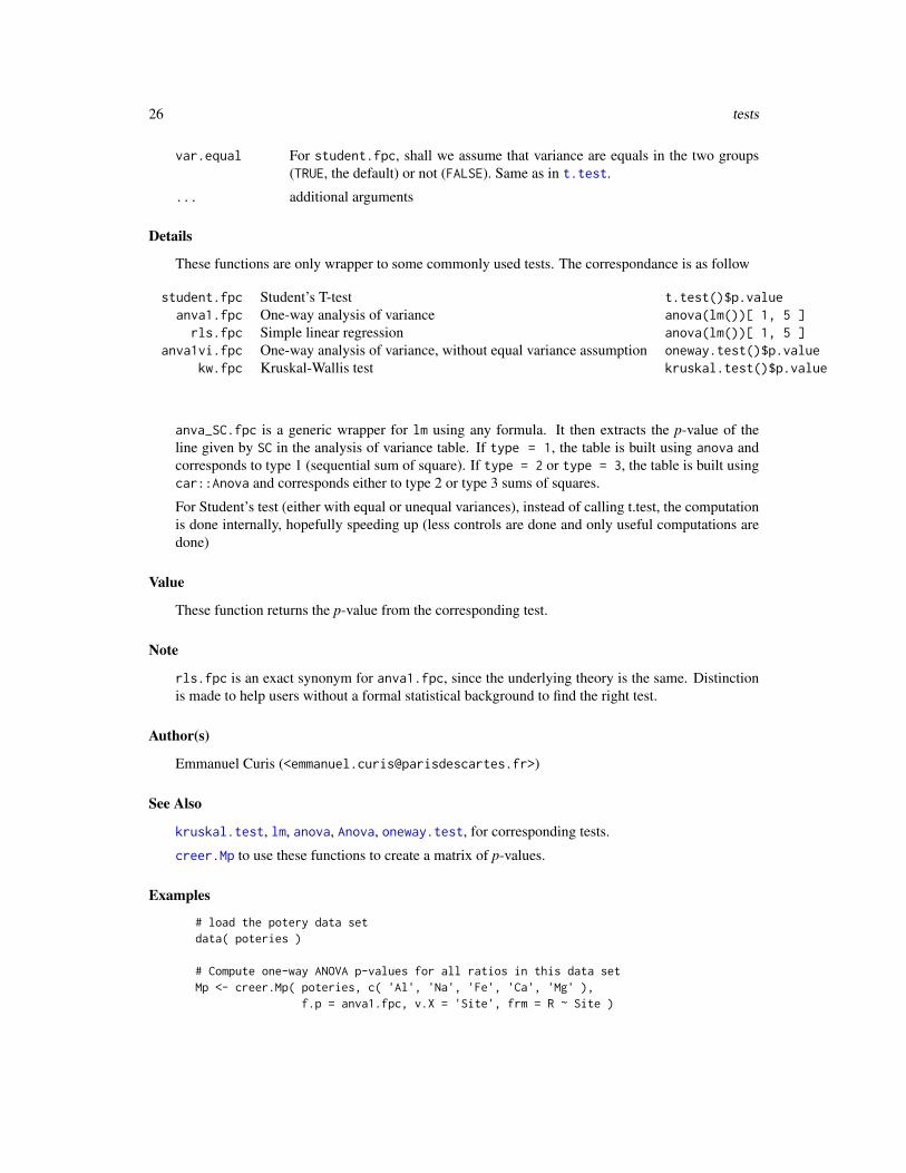
var.equal For student.fpc, shall we assume that variance are equals in the two groups(TRUE, the default) or not (FALSE). Same as in t.test.

... additional arguments

Details

These functions are only wrapper to some commonly used tests. The correspondance is as follow

student.fpc Student’s T-test t.test()$p.valueanva1.fpc One-way analysis of variance anova(lm())[ 1, 5 ]rls.fpc Simple linear regression anova(lm())[ 1, 5 ]

anva1vi.fpc One-way analysis of variance, without equal variance assumption oneway.test()$p.valuekw.fpc Kruskal-Wallis test kruskal.test()$p.value

anva_SC.fpc is a generic wrapper for lm using any formula. It then extracts the p-value of theline given by SC in the analysis of variance table. If type = 1, the table is built using anova andcorresponds to type 1 (sequential sum of square). If type = 2 or type = 3, the table is built usingcar::Anova and corresponds either to type 2 or type 3 sums of squares.

For Student’s test (either with equal or unequal variances), instead of calling t.test, the computationis done internally, hopefully speeding up (less controls are done and only useful computations aredone)

Value

These function returns the p-value from the corresponding test.

Note

rls.fpc is an exact synonym for anva1.fpc, since the underlying theory is the same. Distinctionis made to help users without a formal statistical background to find the right test.

Author(s)


See Also

kruskal.test, lm, anova, Anova, oneway.test, for corresponding tests.

creer.Mp to use these functions to create a matrix of p-values.

Examples



f.p = anva1.fpc, v.X = 'Site', frm = R ~ Site )

tests 27

Mp


Index

∗Topic \textasciitildekwd1calc.rapports, 5

∗Topic \textasciitildekwd2calc.rapports, 5

∗Topic compositionalarbre.Mp, 2choisir.seuil, 6conversions, 8coupures.Mp, 10creer_data.frame, 12creer_graphe, 14creer_matrice, 16modele, 18puissance, 21tests, 25

∗Topic datasetsBpLi, 4poteries, 20

alpha (puissance), 21Anova, 26anova, 26anva1.fpc, 13, 17anva1.fpc (tests), 25anva1vi.fpc (tests), 25anva_SC.fpc (tests), 25arbre.Mp, 2, 11as.data.frame, 5, 12, 16as.dendrogram, 3

BpLi, 4BpLi_J2 (BpLi), 4BpLi_J4 (BpLi), 4

calc.rapports, 5choisir.seuil, 2, 6, 10, 24components, 19conversions, 8coupures.Mp, 3, 10create.DFp (creer_data.frame), 12

create.graphe (creer_graphe), 14create.Mp (creer_matrice), 16creer.DFp, 9, 15creer.DFp (creer_data.frame), 12creer.Mp, 3, 6–9, 11–13, 15, 22, 24, 26creer.Mp (creer_matrice), 16creer_data.frame, 12creer_graphe, 14creer_matrice, 16

DFp.Mp (conversions), 8

estimer.alpha, 19estimer.alpha (puissance), 21estimer.puissance, 19estimer.puissance (puissance), 21

grf.DFp, 13grf.DFp (creer_graphe), 14grf.Mp, 3, 11, 17grf.Mp (creer_graphe), 14

kruskal.test, 26kw.fpc, 13, 17kw.fpc (tests), 25

lm, 26

make.names, 12, 16modele, 18modele_compo, 22, 24modele_compo (modele), 18Mp.DFp (conversions), 8

oneway.test, 26

plot, 10, 18plot.Arbre (arbre.Mp), 2plot.Coupures (coupures.Mp), 10plot.dendrogram, 3plot.SARPcompo.H0 (choisir.seuil), 6

28

INDEX 29

plot.SARPcompo.modele (modele), 18poteries, 20print.SARPcompo.H0 (choisir.seuil), 6puissance, 21

read.table, 9rls.fpc (tests), 25

student.fpc (tests), 25

t.test, 26tests, 25

write.table, 9

Documents

Package ‘SARP.compo’ - cran.r-project.org · Package ‘SARP.compo’ May 21, 2018 Type Package Title Network-based Interpretation of Changes in Compositional Data Version 0.0.7