Package ‘rr’ - The Comprehensive R Archive Network · Package ‘rr’ August 17, 2016 Version 1.4 Date 2016-8-15 Title Statistical Methods for the Randomized Response Technique

Package ‘rr’August 17, 2016

Version 1.4

Date 2016-8-15

Title Statistical Methods for the Randomized Response Technique

Author Graeme Blair [aut, cre], Yang-Yang Zhou [aut, cre],Kosuke Imai [aut, cre], Winston Chou [ctb]

Maintainer Graeme Blair <[email protected]>

Depends R (>= 3.0.0), utils

Imports MASS, arm, coda, magic

Description Enables researchers to conduct multivariate statistical analysesof survey data with randomized response technique items from several designs,including mirrored question, forced question, and unrelated question. Thisincludes regression with the randomized response as the outcome and logisticregression with the randomized response item as a predictor. In addition,tools for conducting power analysis for designing randomized response itemsare included. The package implements methods described in Blair, Imai, and Zhou(2015) ''Design and Analysis of the Randomized Response Technique,'' Journalof the American Statistical Association<http://graemeblair.com/papers/randresp.pdf>.

LazyLoad yes

LazyData yes

License GPL (>= 3)

Suggests testthat

RoxygenNote 5.0.1

NeedsCompilation yes

Repository CRAN

Date/Publication 2016-08-17 00:49:19

R topics documented:rr-package . . . . . . . . . . . . . . . . . . . . . . . . . . . . . . . . . . . . . . . . . . 2nigeria . . . . . . . . . . . . . . . . . . . . . . . . . . . . . . . . . . . . . . . . . . . . 3

1

2 rr-package

nigeria-data . . . . . . . . . . . . . . . . . . . . . . . . . . . . . . . . . . . . . . . . . 4power.rr.plot . . . . . . . . . . . . . . . . . . . . . . . . . . . . . . . . . . . . . . . . . 5power.rr.test . . . . . . . . . . . . . . . . . . . . . . . . . . . . . . . . . . . . . . . . . 7predict.rrreg . . . . . . . . . . . . . . . . . . . . . . . . . . . . . . . . . . . . . . . . . 10predict.rrreg.predictor . . . . . . . . . . . . . . . . . . . . . . . . . . . . . . . . . . . . 12rrreg . . . . . . . . . . . . . . . . . . . . . . . . . . . . . . . . . . . . . . . . . . . . . 14rrreg.bayes . . . . . . . . . . . . . . . . . . . . . . . . . . . . . . . . . . . . . . . . . 17rrreg.predictor . . . . . . . . . . . . . . . . . . . . . . . . . . . . . . . . . . . . . . . . 20

Index 24

rr-package R Package for the Randomized Response Technique

Description

rr implements methods developed by Blair, Imai, and Zhou (2015) such as multivariate regres-sion and power analysis for the randomized response technique. Randomized response is a surveytechnique that introduces random noise to reduce potential bias from non-response and social de-sirability when asking questions about sensitive behaviors and beliefs. The current version of thispackage conducts multivariate regression analyses for the sensitive item under four standard ran-domized response designs: mirrored question, forced response, disguised response, and unrelatedquestion. Second, it generates predicted probabilities of answering affirmatively to the sensitiveitem for each respondent. Third, it also allows users to use the sensitive item as a predictor in anoutcome regression under the forced response design. Additionally, it implements power analysesto help improve research design. In future versions, this package will extend to new modified de-signs that are based on less stringent assumptions than those of the standard designs, specifically toallow for non-compliance and unknown distribution to the unrelated question under the unrelatedquestion design.

Details

Package: rrType: PackageVersion: 1.2Date: 2015-3-8License: GPL (>= 2)

Author(s)

Graeme Blair, Experiments in Governance and Politics, Columbia University <[email protected]>,http://graemeblair.com

Kosuke Imai, Department of Politics, Princeton University <[email protected]>, http://imai.princeton.edu

http://graemeblair.com

http://imai.princeton.edu

http://imai.princeton.edu

nigeria 3

Yang-Yang Zhou, Department of Politics, Princeton University <[email protected]>, http://yangyangzhou.com

Maintainer: Graeme Blair <[email protected]>

References

Blair, Graeme, Kosuke Imai and Yang-Yang Zhou. (2015) "Design and Analysis of the Random-ized Response Technique." Journal of the American Statistical Association. Available at http://graemeblair.com/papers/randresp.pdf.

nigeria Nigeria Randomized Response Survey Experiment on Social Connec-tions to Armed Groups

Description

This data set is a subset of the data from the randomized response technique survey experimentconducted in Nigeria to study civilian contact with armed groups. The survey was implemented byBlair (2014).

Usage

data(nigeria)

Format

A data frame containing 2457 observations. The variables are:

• Quesid: Survey ID of civilian respondent.

• rr.q1: Randomized response survey item using the Forced Response Design asking the re-spondent whether they hold direct social connections with members of armed groups. 0 if noconnection; 1 if connection.

• cov.age: Age of the respondent.

• cov.asset.index: The number of assets owned by the respondent from an index of nineassets including radio, T.V., motorbike, car, mobile phone, refrigerator, goat, chicken, andcow.

• cov.married: Marital status. 0 if single; 1 if married.

• cov.education: Education level of the respondent. 1 if no school; 2 if started primary school;3 if finished primary school; 4 if started secondary school; 5 if finished secondary school; 6 ifstarted polytechnic or college; 7 if finished polytechnic or college; 8 if started university; 9 iffinished university; 10 if received graduate (masters or Ph.D) education.

• cov.female: Gender. 0 if male; 1 if female.

• civic: Whether or not the respondent is a member of a civic group in their communities, suchas youth groups , women’s groups, or community development committees.

http://yangyangzhou.com

http://yangyangzhou.com

http://graemeblair.com/papers/randresp.pdf


4 nigeria-data

Source

Blair, Graeme, Kosuke Imai and Yang-Yang Zhou. (2014) Replication data for: Design and Analy-sis of the Randomized Response Technique.

References

Blair, G. (2014). "Why do civilians hold bargaining power in state revenue conflicts? Evidencefrom Nigeria."

Blair, Graeme, Kosuke Imai and Yang-Yang Zhou. (2014) "Design and Analysis of the RandomizedResponse Technique." Working Paper. Available at http://imai.princeton.edu/research/randresp.html.

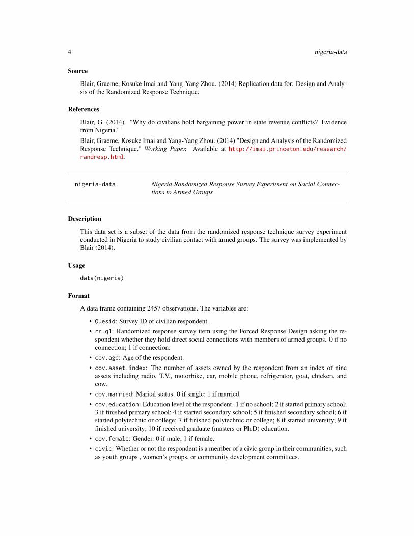
nigeria-data Nigeria Randomized Response Survey Experiment on Social Connec-tions to Armed Groups

Description

This data set is a subset of the data from the randomized response technique survey experimentconducted in Nigeria to study civilian contact with armed groups. The survey was implemented byBlair (2014).

Usage

data(nigeria)

Format

A data frame containing 2457 observations. The variables are:

• Quesid: Survey ID of civilian respondent.• rr.q1: Randomized response survey item using the Forced Response Design asking the re-

spondent whether they hold direct social connections with members of armed groups. 0 if noconnection; 1 if connection.

• cov.age: Age of the respondent.• cov.asset.index: The number of assets owned by the respondent from an index of nine

assets including radio, T.V., motorbike, car, mobile phone, refrigerator, goat, chicken, andcow.

• cov.married: Marital status. 0 if single; 1 if married.• cov.education: Education level of the respondent. 1 if no school; 2 if started primary school;

3 if finished primary school; 4 if started secondary school; 5 if finished secondary school; 6 ifstarted polytechnic or college; 7 if finished polytechnic or college; 8 if started university; 9 iffinished university; 10 if received graduate (masters or Ph.D) education.

• cov.female: Gender. 0 if male; 1 if female.• civic: Whether or not the respondent is a member of a civic group in their communities, such

as youth groups , women’s groups, or community development committees.

http://imai.princeton.edu/research/randresp.html


power.rr.plot 5

Source

Blair, Graeme, Kosuke Imai and Yang-Yang Zhou. (2014) Replication data for: Design and Analy-sis of the Randomized Response Technique.

References

Blair, G. (2014). "Why do civilians hold bargaining power in state revenue conflicts? Evidencefrom Nigeria."


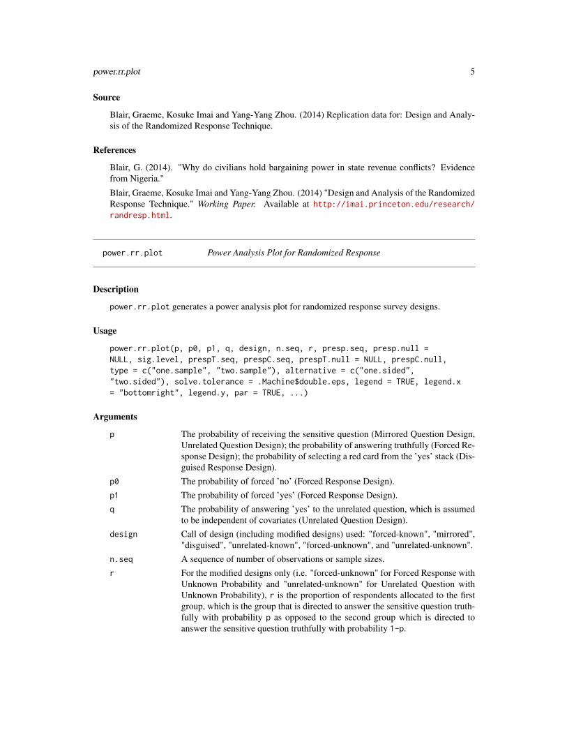
power.rr.plot Power Analysis Plot for Randomized Response

Description

power.rr.plot generates a power analysis plot for randomized response survey designs.

Usage

power.rr.plot(p, p0, p1, q, design, n.seq, r, presp.seq, presp.null =NULL, sig.level, prespT.seq, prespC.seq, prespT.null = NULL, prespC.null,type = c("one.sample", "two.sample"), alternative = c("one.sided","two.sided"), solve.tolerance = .Machine$double.eps, legend = TRUE, legend.x= "bottomright", legend.y, par = TRUE, ...)

Arguments

p The probability of receiving the sensitive question (Mirrored Question Design,Unrelated Question Design); the probability of answering truthfully (Forced Re-sponse Design); the probability of selecting a red card from the ’yes’ stack (Dis-guised Response Design).

p0 The probability of forced ’no’ (Forced Response Design).p1 The probability of forced ’yes’ (Forced Response Design).q The probability of answering ’yes’ to the unrelated question, which is assumed

to be independent of covariates (Unrelated Question Design).design Call of design (including modified designs) used: "forced-known", "mirrored",

"disguised", "unrelated-known", "forced-unknown", and "unrelated-unknown".n.seq A sequence of number of observations or sample sizes.r For the modified designs only (i.e. "forced-unknown" for Forced Response with

Unknown Probability and "unrelated-unknown" for Unrelated Question withUnknown Probability), r is the proportion of respondents allocated to the firstgroup, which is the group that is directed to answer the sensitive question truth-fully with probability p as opposed to the second group which is directed toanswer the sensitive question truthfully with probability 1-p.



6 power.rr.plot

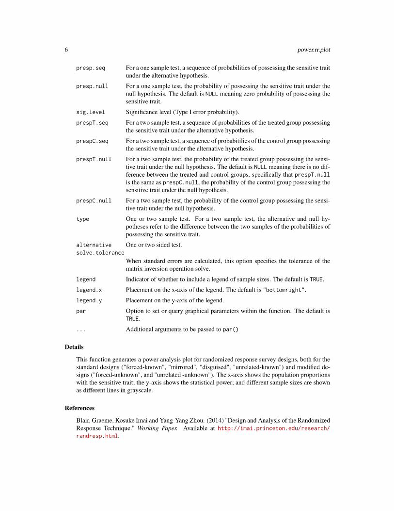
presp.seq For a one sample test, a sequence of probabilities of possessing the sensitive traitunder the alternative hypothesis.

presp.null For a one sample test, the probability of possessing the sensitive trait under thenull hypothesis. The default is NULL meaning zero probability of possessing thesensitive trait.

sig.level Significance level (Type I error probability).

prespT.seq For a two sample test, a sequence of probabilities of the treated group possessingthe sensitive trait under the alternative hypothesis.

prespC.seq For a two sample test, a sequence of probabitilies of the control group possessingthe sensitive trait under the alternative hypothesis.

prespT.null For a two sample test, the probability of the treated group possessing the sensi-tive trait under the null hypothesis. The default is NULL meaning there is no dif-ference between the treated and control groups, specifically that prespT.nullis the same as prespC.null, the probability of the control group possessing thesensitive trait under the null hypothesis.

prespC.null For a two sample test, the probability of the control group possessing the sensi-tive trait under the null hypothesis.

type One or two sample test. For a two sample test, the alternative and null hy-potheses refer to the difference between the two samples of the probabilities ofpossessing the sensitive trait.

alternative One or two sided test.solve.tolerance

When standard errors are calculated, this option specifies the tolerance of thematrix inversion operation solve.

legend Indicator of whether to include a legend of sample sizes. The default is TRUE.

legend.x Placement on the x-axis of the legend. The default is "bottomright".

legend.y Placement on the y-axis of the legend.

par Option to set or query graphical parameters within the function. The default isTRUE.

... Additional arguments to be passed to par()

Details

This function generates a power analysis plot for randomized response survey designs, both for thestandard designs ("forced-known", "mirrored", "disguised", "unrelated-known") and modified de-signs ("forced-unknown", and "unrelated -unknown"). The x-axis shows the population proportionswith the sensitive trait; the y-axis shows the statistical power; and different sample sizes are shownas different lines in grayscale.

References




power.rr.test 7

Examples

## Generate a power plot for the forced design with known## probabilities of 2/3 in truth-telling group, 1/6 forced to say "yes"## and 1/6 forced to say "no", varying the number of respondents from## 250 to 2500 and the population proportion of respondents## possessing the sensitive trait from 0 to .15.

presp.seq <- seq(from = 0, to = .15, by = .0025)n.seq <- c(250, 500, 1000, 2000, 2500)power.rr.plot(p = 2/3, p1 = 1/6, p0 = 1/6, n.seq = n.seq,

presp.seq = presp.seq, presp.null = 0,design = "forced-known", sig.level = .01,type = "one.sample",alternative = "one.sided", legend = TRUE)

## Replicates the results for Figure 2 in Blair, Imai, and Zhou (2014)

power.rr.test Power Analysis for Randomized Response

Description

power.rr.test is used to conduct power analysis for randomized response survey designs.

Usage

power.rr.test(p, p0, p1, q, design, n = NULL, r, presp, presp.null =NULL, sig.level, prespT, prespC, prespT.null = NULL, prespC.null, power =NULL, type = c("one.sample", "two.sample"), alternative = c("one.sided","two.sided"), solve.tolerance = .Machine$double.eps)

Arguments


p0 The probability of forced ’no’ (Forced Response Design).

p1 The probability of forced ’yes’ (Forced Response Design).

q The probability of answering ’yes’ to the unrelated question, which is assumedto be independent of covariates (Unrelated Question Design).

design Call of design (including modified designs) used: "forced-known", "mirrored","disguised", "unrelated-known", "forced-unknown", and "unrelated-unknown".

8 power.rr.test

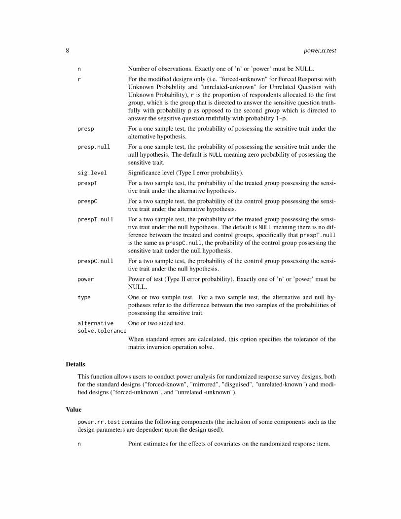
n Number of observations. Exactly one of ’n’ or ’power’ must be NULL.

r For the modified designs only (i.e. "forced-unknown" for Forced Response withUnknown Probability and "unrelated-unknown" for Unrelated Question withUnknown Probability), r is the proportion of respondents allocated to the firstgroup, which is the group that is directed to answer the sensitive question truth-fully with probability p as opposed to the second group which is directed toanswer the sensitive question truthfully with probability 1-p.

presp For a one sample test, the probability of possessing the sensitive trait under thealternative hypothesis.

presp.null For a one sample test, the probability of possessing the sensitive trait under thenull hypothesis. The default is NULL meaning zero probability of possessing thesensitive trait.


prespT For a two sample test, the probability of the treated group possessing the sensi-tive trait under the alternative hypothesis.

prespC For a two sample test, the probability of the control group possessing the sensi-tive trait under the alternative hypothesis.

prespT.null For a two sample test, the probability of the treated group possessing the sensi-tive trait under the null hypothesis. The default is NULL meaning there is no dif-ference between the treated and control groups, specifically that prespT.nullis the same as prespC.null, the probability of the control group possessing thesensitive trait under the null hypothesis.

prespC.null For a two sample test, the probability of the control group possessing the sensi-tive trait under the null hypothesis.

power Power of test (Type II error probability). Exactly one of ’n’ or ’power’ must beNULL.

type One or two sample test. For a two sample test, the alternative and null hy-potheses refer to the difference between the two samples of the probabilities ofpossessing the sensitive trait.

alternative One or two sided test.solve.tolerance


Details

This function allows users to conduct power analysis for randomized response survey designs, bothfor the standard designs ("forced-known", "mirrored", "disguised", "unrelated-known") and modi-fied designs ("forced-unknown", and "unrelated -unknown").

Value

power.rr.test contains the following components (the inclusion of some components such as thedesign parameters are dependent upon the design used):

n Point estimates for the effects of covariates on the randomized response item.

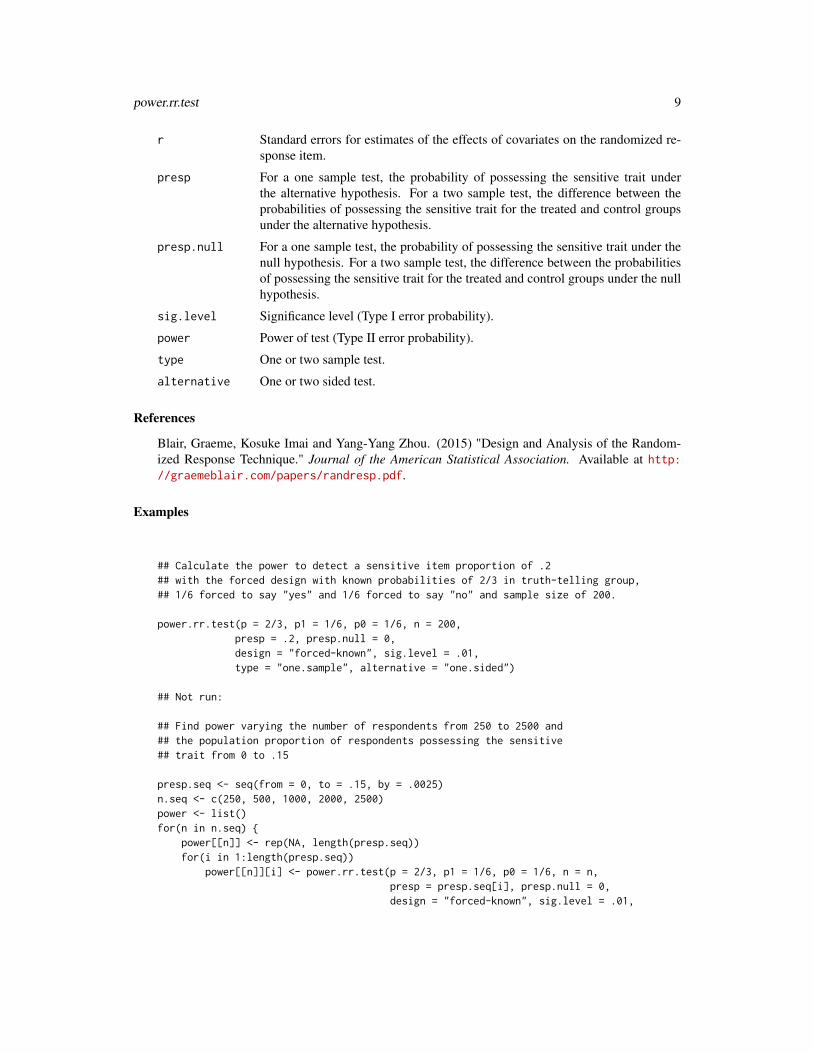
power.rr.test 9

r Standard errors for estimates of the effects of covariates on the randomized re-sponse item.

presp For a one sample test, the probability of possessing the sensitive trait underthe alternative hypothesis. For a two sample test, the difference between theprobabilities of possessing the sensitive trait for the treated and control groupsunder the alternative hypothesis.

presp.null For a one sample test, the probability of possessing the sensitive trait under thenull hypothesis. For a two sample test, the difference between the probabilitiesof possessing the sensitive trait for the treated and control groups under the nullhypothesis.


power Power of test (Type II error probability).

type One or two sample test.

alternative One or two sided test.

References

Blair, Graeme, Kosuke Imai and Yang-Yang Zhou. (2015) "Design and Analysis of the Random-ized Response Technique." Journal of the American Statistical Association. Available at http://graemeblair.com/papers/randresp.pdf.

Examples

## Calculate the power to detect a sensitive item proportion of .2## with the forced design with known probabilities of 2/3 in truth-telling group,## 1/6 forced to say "yes" and 1/6 forced to say "no" and sample size of 200.

power.rr.test(p = 2/3, p1 = 1/6, p0 = 1/6, n = 200,presp = .2, presp.null = 0,design = "forced-known", sig.level = .01,type = "one.sample", alternative = "one.sided")

## Not run:

## Find power varying the number of respondents from 250 to 2500 and## the population proportion of respondents possessing the sensitive## trait from 0 to .15

presp.seq <- seq(from = 0, to = .15, by = .0025)n.seq <- c(250, 500, 1000, 2000, 2500)power <- list()for(n in n.seq) {

power[[n]] <- rep(NA, length(presp.seq))for(i in 1:length(presp.seq))

power[[n]][i] <- power.rr.test(p = 2/3, p1 = 1/6, p0 = 1/6, n = n,presp = presp.seq[i], presp.null = 0,design = "forced-known", sig.level = .01,



10 predict.rrreg

type = "one.sample",alternative = "one.sided")$power

}

## Replicates the results for Figure 2 in Blair, Imai, and Zhou (2014)

## End(Not run)

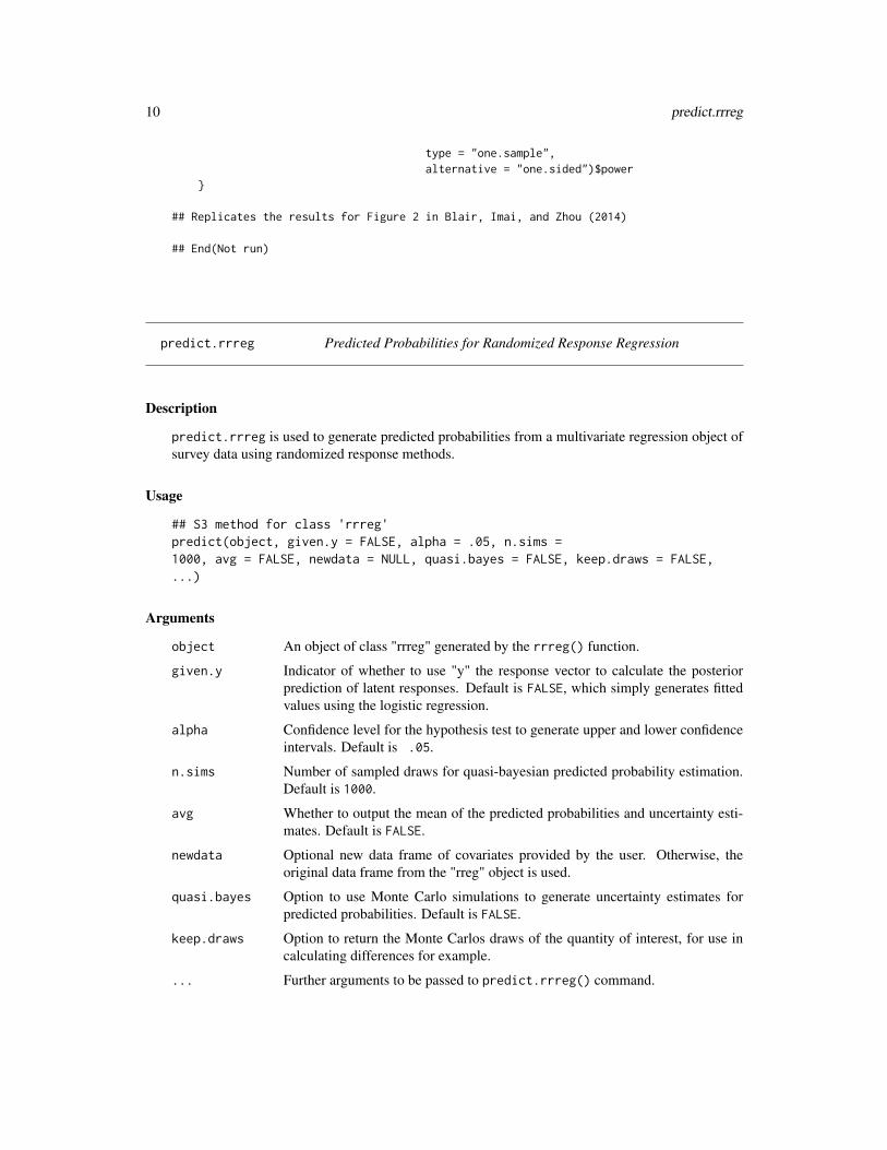
predict.rrreg Predicted Probabilities for Randomized Response Regression

Description

predict.rrreg is used to generate predicted probabilities from a multivariate regression object ofsurvey data using randomized response methods.

Usage

## S3 method for class 'rrreg'predict(object, given.y = FALSE, alpha = .05, n.sims =1000, avg = FALSE, newdata = NULL, quasi.bayes = FALSE, keep.draws = FALSE,...)

Arguments

object An object of class "rrreg" generated by the rrreg() function.

given.y Indicator of whether to use "y" the response vector to calculate the posteriorprediction of latent responses. Default is FALSE, which simply generates fittedvalues using the logistic regression.

alpha Confidence level for the hypothesis test to generate upper and lower confidenceintervals. Default is .05.

n.sims Number of sampled draws for quasi-bayesian predicted probability estimation.Default is 1000.

avg Whether to output the mean of the predicted probabilities and uncertainty esti-mates. Default is FALSE.

newdata Optional new data frame of covariates provided by the user. Otherwise, theoriginal data frame from the "rreg" object is used.

quasi.bayes Option to use Monte Carlo simulations to generate uncertainty estimates forpredicted probabilities. Default is FALSE.

keep.draws Option to return the Monte Carlos draws of the quantity of interest, for use incalculating differences for example.

... Further arguments to be passed to predict.rrreg() command.

predict.rrreg 11

Details

This function allows users to generate predicted probabilities for the randomized response itemgiven an object of class "rrreg" from the rrreg() function. Four standard designs are accepted bythis function: mirrored question, forced response, disguised response, and unrelated question. Thedesign, already specified in the "rrreg" object, is then directly inputted into this function.

Value

predict.rrreg returns predicted probabilities either for each observation in the data frame or theaverage over all observations. The output is a list that contains the following components:

est Predicted probabilities for the randomized response item generated either usingfitted values, posterior predictions, or quasi-Bayesian simulations. If avg is setto TRUE, the output will only include the mean estimate.

se Standard errors for the predicted probabilities of the randomized response itemgenerated using Monte Carlo simulations. If quasi.bayes is set to FALSE, nostandard errors will be outputted.

ci.lower Estimates for the lower confidence interval. If quasi.bayes is set to FALSE, noconfidence interval estimate will be outputted.

ci.upper Estimates for the upper confidence interval. If quasi.bayes is set to FALSE, noconfidence interval estimate will be outputted.

qoi.draws Monte Carlos draws of the quantity of interest, returned only if keep.draws isset to TRUE.

References


See Also

rrreg to conduct multivariate regression analyses in order to generate predicted probabilities forthe randomized response item.

Examples

## Not run:data(nigeria)

set.seed(1)

## Define design parametersp <- 2/3 # probability of answering honestly in Forced Response Designp1 <- 1/6 # probability of forced 'yes'p0 <- 1/6 # probability of forced 'no'

## Fit linear regression on the randomized response item of



12 predict.rrreg.predictor

## whether citizen respondents had direct social contacts to armed groups

rr.q1.reg.obj <- rrreg(rr.q1 ~ cov.asset.index + cov.married + I(cov.age/10) +I((cov.age/10)^2) + cov.education + cov.female,data = nigeria, p = p, p1 = p1, p0 = p0,design = "forced-known")

## Generate the mean predicted probability of having social contacts to## armed groups across respondents using quasi-Bayesian simulations.

rr.q1.reg.pred <- predict(rr.q1.reg.obj, given.y = FALSE,avg = TRUE, quasi.bayes = TRUE,n.sims = 10000)

## Replicates Table 3 in Blair, Imai, and Zhou (2014)

## End(Not run)

predict.rrreg.predictor

Predicted Probabilities for Randomized Response as a RegressionPredictor

Description

predict.rrreg.predictor is used to generate predicted probabilities from a multivariate regres-sion object of survey data using the randomized response item as a predictor for an additionaloutcome.

Usage

predict.rrreg.predictor(object, fix.z = NULL, alpha = .05,n.sims = 1000, avg = FALSE, newdata = NULL, quasi.bayes = FALSE, keep.draws= FALSE, ...)

Arguments

object An object of class "rrreg.predictor" generated by the rrreg.predictor() func-tion.

fix.z An optional value or vector of values between 0 and 1 that the user inputs as theproportion of respondents with the sensitive trait or probability that each respon-dent has the sensitive trait, respectively. If the user inputs a vector of values, thevector must be the length of the data from the "rrreg.predictor" object. Defaultis NULL in which case predicted probabilities are generated for the randomizedresponse item.

alpha Confidence level for the hypothesis test to generate upper and lower confidenceintervals. Default is .05.

predict.rrreg.predictor 13

n.sims Number of sampled draws for quasi-bayesian predicted probability estimation.Default is 1000.

avg Whether to output the mean of the predicted probabilities and uncertainty esti-mates. Default is FALSE.

newdata Optional new data frame of covariates provided by the user. Otherwise, theoriginal data frame from the "rreg" object is used.

quasi.bayes Option to use Monte Carlo simulations to generate uncertainty estimates forpredicted probabilities. Default is FALSE meaning no uncertainty estimates areoutputted.

keep.draws Option to return the Monte Carlos draws of the quantity of interest, for use incalculating differences for example.

... Further arguments to be passed to predict.rrreg.predictor() command.

Details

This function allows users to generate predicted probabilities for the additional outcome variableswith the randomized response item as a covariate given an object of class "rrreg.predictor" fromthe rrreg.predictor() function. Four standard designs are accepted by this function: mirroredquestion, forced response, disguised response, and unrelated question. The design, already specifiedin the "rrreg.predictor" object, is then directly inputted into this function.

Value

predict.rrreg.predictor returns predicted probabilities either for each observation in the dataframe or the average over all observations. The output is a list that contains the following compo-nents:

est Predicted probabilities of the additional outcome variable given the random-ized response item as a predictor generated either using fitted values or quasi-Bayesian simulations. If avg is set to TRUE, the output will only include themean estimate.

se Standard errors for the predicted probabilities of the additional outcome vari-able given the randomized response item as a predictor generated using MonteCarlo simulations. If quasi.bayes is set to FALSE, no standard errors will beoutputted.

ci.lower Estimates for the lower confidence interval. If quasi.bayes is set to FALSE, noconfidence interval estimate will be outputted.

ci.upper Estimates for the upper confidence interval. If quasi.bayes is set to FALSE, noconfidence interval estimate will be outputted.

qoi.draws Monte Carlos draws of the quantity of interest, returned only if keep.draws isset to TRUE.

References




14 rrreg

See Also

rrreg.predictor to conduct multivariate regression analyses with the randomized response aspredictor in order to generate predicted probabilities.

Examples

## Not run:data(nigeria)

## Define design parameters

set.seed(44)

p <- 2/3 # probability of answering honestly in Forced Response Designp1 <- 1/6 # probability of forced 'yes'p0 <- 1/6 # probability of forced 'no'

## Fit joint model of responses to an outcome regression of joining a civic## group and the randomized response item of having a militant social connection

rr.q1.pred.obj <-rrreg.predictor(civic ~ cov.asset.index + cov.married + I(cov.age/10) +

I((cov.age/10)^2) + cov.education + cov.female+ rr.q1, rr.item = "rr.q1", parstart = FALSE, estconv = TRUE,data = nigeria, verbose = FALSE, optim = TRUE,p = p, p1 = p1, p0 = p0, design = "forced-known")

## Generate predicted probabilities for the likelihood of joining## a civic group across respondents using quasi-Bayesian simulations.

rr.q1.rrreg.predictor.pred <- predict(rr.q1.pred.obj,avg = TRUE, quasi.bayes = TRUE,n.sims = 10000)

## End(Not run)

rrreg Randomized Response Regression

Description

rrreg is used to conduct multivariate regression analyses of survey data using randomized responsemethods.

rrreg 15

Usage

rrreg(formula, p, p0, p1, q, design, data, start = NULL,h = NULL, group = NULL, matrixMethod = "efficient",maxIter = 10000, verbose = FALSE, optim = FALSE, em.converge = 10^(-8),glmMaxIter = 10000, solve.tolerance = .Machine$double.eps)

Arguments

formula An object of class "formula": a symbolic description of the model to be fitted.p The probability of receiving the sensitive question (Mirrored Question Design,

Unrelated Question Design); the probability of answering truthfully (Forced Re-sponse Design); the probability of selecting a red card from the ’yes’ stack (Dis-guised Response Design). For "mirrored" and "disguised" designs, p cannotequal .5.

p0 The probability of forced ’no’ (Forced Response Design).p1 The probability of forced ’yes’ (Forced Response Design).q The probability of answering ’yes’ to the unrelated question, which is assumed

to be independent of covariates (Unrelated Question Design).design One of the four standard designs: "forced-known", "mirrored", "disguised", or

"unrelated-known".data A data frame containing the variables in the model.start Optional starting values of coefficient estimates for the Expectation-Maximization

(EM) algorithm.h Auxiliary data functionality. Optional named numeric vector with length equal

to number of groups. Names correspond to group labels and values correspondto auxiliary moments.

group Auxiliary data functionality. Optional character vector of group labels withlength equal to number of observations.

matrixMethod Auxiliary data functionality. Procedure for estimating optimal weighting matrixfor generalized method of moments. One of "efficient" for two-step feasible and"cue" for continuously updating. Default is "efficient". Only relevant if h andgroup are specified.

maxIter Maximum number of iterations for the Expectation-Maximization algorithm.The default is 10000.

verbose A logical value indicating whether model diagnostics counting the number ofEM iterations are printed out. The default is FALSE.

optim A logical value indicating whether to use the quasi-Newton "BFGS" methodto calculate the variance-covariance matrix and standard errors. The default isFALSE.

em.converge A value specifying the satisfactory degree of convergence under the EM algo-rithm. The default is 10^(-8).

glmMaxIter A value specifying the maximum number of iterations to run the EM algorithm.The default is 10000.

solve.tolerance


16 rrreg

Details

This function allows users to perform multivariate regression analysis on data from the randomizedresponse technique. Four standard designs are accepted by this function: mirrored question, forcedresponse, disguised response, and unrelated question. The method implemented by this function isthe Maximum Likelihood (ML) estimation for the Expectation-Maximization (EM) algorithm.

Value

rrreg returns an object of class "rrreg". The function summary is used to obtain a table of theresults. The object rrreg is a list that contains the following components (the inclusion of somecomponents such as the design parameters are dependent upon the design used):

est Point estimates for the effects of covariates on the randomized response item.

vcov Variance-covariance matrix for the effects of covariates on the randomized re-sponse item.

se Standard errors for estimates of the effects of covariates on the randomized re-sponse item.

data The data argument.

coef.names Variable names as defined in the data frame.

x The model matrix of covariates.

y The randomized response vector.

design Call of standard design used: "forced-known", "mirrored", "disguised", or "unrelated-known".

p The p argument.

p0 The p0 argument.

p1 The p1 argument.

q The q argument.

call The matched call.

References


See Also

predict.rrreg for predicted probabilities.

Examples

data(nigeria)

set.seed(1)



rrreg.bayes 17

## Define design parametersp <- 2/3 # probability of answering honestly in Forced Response Designp1 <- 1/6 # probability of forced 'yes'p0 <- 1/6 # probability of forced 'no'

## Fit linear regression on the randomized response item of whether## citizen respondents had direct social contacts to armed groups

rr.q1.reg.obj <- rrreg(rr.q1 ~ cov.asset.index + cov.married +I(cov.age/10) + I((cov.age/10)^2) + cov.education + cov.female,data = nigeria, p = p, p1 = p1, p0 = p0,design = "forced-known")

summary(rr.q1.reg.obj)

## Replicates Table 3 in Blair, Imai, and Zhou (2014)

rrreg.bayes Bayesian Randomized Response Regression

Description

Function to conduct multivariate regression analyses of survey data with the randomized responsetechnique using Bayesian MCMC.

Usage

rrreg.bayes(formula, p, p0, p1, design, data, group.mixed,formula.mixed = ~1, verbose = FALSE, n.draws = 10000, burnin = 5000, thin =1, beta.start, beta.mu0, beta.A0, beta.tune, Psi.start, Psi.df, Psi.scale,Psi.tune)

Arguments

formula An object of class "formula": a symbolic description of the model to be fitted.




design Character indicating the design. Currently only "forced-known" is supported.

data A data frame containing the variables in the model.

group.mixed A string indicating the variable name of a numerical group indicator specifyingwhich group each individual belongs to for a mixed effects model.

18 rrreg.bayes

formula.mixed To specify a mixed effects model, include this formula object for the group-levelfit. ~1 allows intercepts to vary, and including covariates in the formula allowsthe slopes to vary also.

verbose A logical value indicating whether model diagnostics are printed out during fit-ting.

n.draws Number of MCMC iterations.

burnin The number of initial MCMC iterations that are discarded.

thin The interval of thinning between consecutive retained iterations (1 for no thin-ning).

beta.start Optional starting values for the sensitive item fit. This should be a vector oflength the number of covariates.

beta.mu0 Optional vector of prior means for the sensitive item fit parameters, a vector oflength the number of covariates.

beta.A0 Optional matrix of prior precisions for the sensitive item fit parameters, a matrixof dimension the number of covariates.

beta.tune A required vector of tuning parameters for the Metropolis algorithm for the sen-sitive item fit. This must be set and refined by the user until the acceptance ratiosare approximately .4 (reported in the output).

Psi.start Optional starting values for the variance of the random effects in the mixedeffects models. This should be a scalar.

Psi.df Optional prior degrees of freedom parameter for the variance of the randomeffects in the mixed effects models.

Psi.scale Optional prior scale parameter for the variance of the random effects in themixed effects models.

Psi.tune A required vector of tuning parameters for the Metropolis algorithm for vari-ance of the random effects in the mixed effects models. This must be set andrefined by the user until the acceptance ratios are approximately .4 (reported inthe output).

Details

This function allows the user to perform regression analysis on data from the randomized responsetechnique using a Bayesian MCMC algorithm.

The Metropolis algorithm for the Bayesian MCMC estimators in this function must be tuned to workcorrectly. The beta.tune and, for the mixed effects model Psi.tune, are required, and the values,one for each estimated parameter, will need to be manipulated. The output of the rrreg.bayesfunction displays the acceptance ratios from the Metropolis algorithm. If these values are far from0.4, the tuning parameters should be changed until the ratios approach 0.4.

Convergence is at times difficult to achieve, so we recommend running multiple chains from overdis-persed starting values by, for example, running an MLE using the rrreg() function, and then gen-erating a set of overdispersed starting values using those estimates and their estimated variance-covariance matrix. An example is provided below for each of the possible designs. Runningsummary() after such a procedure will output the Gelman-Rubin convergence statistics in additionto the estimates. If the G-R statistics are all below 1.1, the model is said to have converged.

rrreg.bayes 19

Value

rrreg.bayes returns an object of class "rrreg.bayes". The function summary is used to obtain atable of the results.

beta The coefficients for the sensitive item fit. An object of class "mcmc" that can beanalyzed using the coda package.






p The p argument.

p0 The p0 argument.

p1 The p1 argument.

beta.tune The beta.tune argument.

mixed Indicator for whether a mixed effects model was run.

call the matched call.

If a mixed-effects model is used, then several additional objects are included:

Psi The coefficients for the group-level fit. An object of class "mcmc" that can beanalyzed using the coda package.

gamma The random effects estimates. An object of class "mcmc" that can be analyzedusing the coda package.

coef.names.mixed

Variable names for the predictors for the second-level model

z The predictors for the second-level model.

groups A vector of group indicators.

Psi.tune The Psi.tune argument.

References


Examples

data(nigeria)

## Define design parametersp <- 2/3 # probability of answering honestly in Forced Response Designp1 <- 1/6 # probability of forced 'yes'



20 rrreg.predictor

p0 <- 1/6 # probability of forced 'no'

## run three chains with overdispersed starting values

set.seed(1)

## starting values constructed from MLE modelmle.estimates <- rrreg(rr.q1 ~ cov.asset.index + cov.married +

I(cov.age/10) + I((cov.age/10)^2) + cov.education + cov.female,data = nigeria,

p = p, p1 = p1, p0 = p0,design = "forced-known")

library(MASS)draws <- mvrnorm(n = 3, mu = coef(mle.estimates),

Sigma = vcov(mle.estimates) * 9)

## Not run:## run three chainsbayes.1 <- rrreg.bayes(rr.q1 ~ cov.asset.index + cov.married +

I(cov.age/10) + I((cov.age/10)^2) + cov.education + cov.female,data = nigeria, p = p, p1 = p1, p0 = p0,beta.tune = .0001, beta.start = draws[1,],design = "forced-known")

bayes.2 <- rrreg.bayes(rr.q1 ~ cov.asset.index + cov.married +I(cov.age/10) + I((cov.age/10)^2) + cov.education + cov.female,

data = nigeria, p = p, p1 = p1, p0 = p0,beta.tune = .0001, beta.start = draws[2,],design = "forced-known")

bayes.3 <- rrreg.bayes(rr.q1 ~ cov.asset.index + cov.married +I(cov.age/10) + I((cov.age/10)^2) + cov.education + cov.female,

data = nigeria, p = p, p1 = p1, p0 = p0,beta.tune = .0001, beta.start = draws[3,],design = "forced-known")

bayes <- as.list(bayes.1, bayes.2, bayes.3)

summary(bayes)

## End(Not run)

rrreg.predictor Randomized Response as a Regression Predictor

Description

rrreg.predictor is used to jointly model the randomized response item as both outcome andpredictor for an additional outcome given a set of covariates.

rrreg.predictor 21

Usage

rrreg.predictor(formula, p, p0, p1, q, design, data, rr.item,model.outcome = "logistic", fit.sens = "bayesglm", fit.outcome = "bayesglm",bstart = NULL, tstart = NULL, parstart = TRUE, maxIter = 10000, verbose =FALSE, optim = FALSE, em.converge = 10^(-4), glmMaxIter = 20000, estconv =TRUE, solve.tolerance = .Machine$double.eps)

Arguments

formula An object of class "formula": a symbolic description of the model to be fittedwith the randomized response item as one of the covariates.




q The probability of answering ’yes’ to the unrelated question, which is assumedto be independent of covariates (Unrelated Question Design).

design One of the four standard designs: "forced-known", "mirrored", "disguised", or"unrelated-known".

data A data frame containing the variables in the model. Observations with missing-ness are list-wise deleted.

rr.item A string containing the name of the randomized response item variable in thedata frame.

model.outcome Currently the function only allows for logistic regression, meaning the outcomevariable must be binary.

fit.sens Indicator for whether to use Bayesian generalized linear modeling (bayesglm)in the Maximization step for the Expectation-Maximization (EM) algorithm togenerate coefficients for the randomized response item as the outcome. Defaultis "bayesglm"; otherwise input "glm".

fit.outcome Indicator for whether to use Bayesian generalized linear modeling (bayesglm)in the Maximization step for the EM algorithm to generate coefficients for theoutcome variable given in the formula with the randomized response item as acovariate. Default is "bayesglm"; otherwise input "glm".

bstart Optional starting values of coefficient estimates for the randomized responseitem as outcome for the EM algorithm.

tstart Optional starting values of coefficient estimates for the outcome variable givenin the formula for the EM algorithm.

parstart Option to use the function rrreg to generate starting values of coefficient esti-mates for the randomized response item as outcome for the EM algorithm. Thedefault is TRUE, but if starting estimates are inputted by the user in bstart, thisoption is overidden.

22 rrreg.predictor

maxIter Maximum number of iterations for the Expectation-Maximization algorithm.The default is 10000.

verbose A logical value indicating whether model diagnostics counting the number ofEM iterations are printed out. The default is FALSE.

optim A logical value indicating whether to use the quasi-Newton "BFGS" methodto calculate the variance-covariance matrix and standard errors. The default isFALSE.

em.converge A value specifying the satisfactory degree of convergence under the EM algo-rithm. The default is 10^(-4).

glmMaxIter A value specifying the maximum number of iterations to run the EM algorithm.The default is 20000 .

estconv Option to base convergence on the absolute value of the difference between sub-sequent coefficients generated through the EM algorithm rather than the subse-quent log-likelihoods. The default is TRUE.

solve.tolerance


Details

This function allows users to perform multivariate regression analysis with the randomized responseitem as a predictor for a separate outcome of interest. It does so by jointly modeling the randomizedresponse item as both outcome and predictor for an additional outcome given the same set of co-variates. Four standard designs are accepted by this function: mirrored question, forced response,disguised response, and unrelated question.

Value

rrreg.predictor returns an object of class "rrpredreg" associated with the randomized responseitem as predictor. The object rrpredreg is a list that contains the following components (theinclusion of some components such as the design parameters are dependent upon the design used):

est.t Point estimates for the effects of the randomized response item as predictor andother covariates on the separate outcome variable specified in the formula.

se.t Standard errors for estimates of the effects of the randomized response itemas predictor and other covariates on the separate outcome variable specified informula.

est.b Point estimates for the effects of covariates on the randomized response item.

vcov Variance-covariance matrix for estimates of the effects of the randomized re-sponse item as predictor and other covariates on the separate outcome variablespecified in formula as well as for estimates of the effects of covariates on therandomized response item.

se.b Standard errors for estimates of the effects of covariates on the randomized re-sponse item.



rrreg.predictor 23



o The separate outcome of interest vector.


p The p argument.

p0 The p0 argument.

p1 The p1 argument.

q The q argument.

call The matched call.

References


See Also

rrreg for multivariate regression.

Examples

data(nigeria)

## Define design parameters

set.seed(44)

p <- 2/3 # probability of answering honestly in Forced Response Designp1 <- 1/6 # probability of forced 'yes'p0 <- 1/6 # probability of forced 'no'

## Fit joint model of responses to an outcome regression of joining a civic## group and the randomized response item of having a militant social connection## Not run:rr.q1.pred.obj <-

rrreg.predictor(civic ~ cov.asset.index + cov.married + I(cov.age/10) +I((cov.age/10)^2) + cov.education + cov.female+ rr.q1, rr.item = "rr.q1", parstart = FALSE, estconv = TRUE,data = nigeria, verbose = FALSE, optim = TRUE,p = p, p1 = p1, p0 = p0, design = "forced-known")

summary(rr.q1.pred.obj)

## End(Not run)## Replicates Table 4 in Blair, Imai, and Zhou (2014)



Index

∗Topic analysispower.rr.plot, 5power.rr.test, 7

∗Topic datasetnigeria, 3nigeria-data, 4

∗Topic fittedpredict.rrreg, 10predict.rrreg.predictor, 12

∗Topic jointrrreg.predictor, 20

∗Topic modelrrreg.predictor, 20

∗Topic packagerr-package, 2

∗Topic powerpower.rr.plot, 5power.rr.test, 7

∗Topic predictedpredict.rrreg, 10predict.rrreg.predictor, 12

∗Topic predictorrrreg.predictor, 20

∗Topic probabilitiespredict.rrreg, 10predict.rrreg.predictor, 12

∗Topic regressionrrreg, 14rrreg.predictor, 20

∗Topic valuespredict.rrreg, 10predict.rrreg.predictor, 12

nigeria, 3nigeria-data, 4

power.rr.plot, 5power.rr.test, 7predict.rrreg, 10, 16predict.rrreg.predictor, 12

rr (rr-package), 2rr-package, 2rrreg, 11, 14, 23rrreg.bayes, 17rrreg.predictor, 14, 20

24

Documents

Package ‘rr’ - The Comprehensive R Archive Network · Package ‘rr’ August 17, 2016 Version 1.4 Date 2016-8-15 Title Statistical Methods for the Randomized Response Technique