Package ‘PReMiuM’ - The Comprehensive R Archive Network · PReMiuM-package 3 Program to implement Dirichlet Process Bayesian Clustering as described in Liverani et al. 2014. This

Package ‘PReMiuM’September 26, 2018

Type Package

Title Dirichlet Process Bayesian Clustering, Profile Regression

Version 3.2.1

Author David I. Hastie, Silvia Liverani <[email protected]> and Sylvia Richardson with contri-butions from Aurore J. Lavigne, Lucy Leigh, Lamiae Azizi, Xi Liu, Ruizhu Huang, Austin Grat-ton, Wei Jing

Maintainer Silvia Liverani <[email protected]>

DescriptionBayesian clustering using a Dirichlet process mixture model. This model is an alternative to re-gression models, non-parametrically linking a response vector to covariate data through clus-ter membership. The package allows Bernoulli, Binomial, Poisson, Normal, survival and categor-ical response, as well as Normal and discrete covariates. It also allows for fixed effects in the re-sponse model, where a spatial CAR (conditional autoregressive) term can be also included. Ad-ditionally, predictions may be made for the response, and missing values for the covari-ates are handled. Several samplers and label switching moves are implemented along with diag-nostic tools to assess convergence. A number of R functions for post-processing of the out-put are also provided. In addition to fitting mixtures, it may additionally be of interest to deter-mine which covariates actively drive the mixture components. This is implemented in the pack-age as variable selection. The main reference for the package is Liverani, Hastie, Azizi, Papath-omas and Richardson (2015) <doi:10.18637/jss.v064.i07>.

URL http://www.silvialiverani.com/software/

License GPL-2

LazyLoad yes

Depends R (>= 3.4.0)

Imports Rcpp (>= 0.12.13), ggplot2 (>= 2.2), cluster, plotrix (>=3.6-6), gamlss.dist (>= 4.3-1), ald (>= 1.1), data.table (>=1.10.4-3), spdep (>= 0.7-7), rgdal (>= 1.3-3)

Suggests testthat (>= 1.0.2)

LinkingTo Rcpp, RcppEigen (>= 0.3.3.3.0), BH (>= 1.65.0-1)

SystemRequirements GNU make

NeedsCompilation yes

1

http://www.silvialiverani.com/software/

2 PReMiuM-package

Repository CRAN

Date/Publication 2018-09-26 14:20:02 UTC

R topics documented:PReMiuM-package . . . . . . . . . . . . . . . . . . . . . . . . . . . . . . . . . . . . . 2calcAvgRiskAndProfile . . . . . . . . . . . . . . . . . . . . . . . . . . . . . . . . . . . 5calcDissimilarityMatrix . . . . . . . . . . . . . . . . . . . . . . . . . . . . . . . . . . . 7calcOptimalClustering . . . . . . . . . . . . . . . . . . . . . . . . . . . . . . . . . . . 8calcPredictions . . . . . . . . . . . . . . . . . . . . . . . . . . . . . . . . . . . . . . . 10clusSummaryBernoulliDiscrete . . . . . . . . . . . . . . . . . . . . . . . . . . . . . . . 13computeRatioOfVariance . . . . . . . . . . . . . . . . . . . . . . . . . . . . . . . . . . 16generateSampleDataFile . . . . . . . . . . . . . . . . . . . . . . . . . . . . . . . . . . 17globalParsTrace . . . . . . . . . . . . . . . . . . . . . . . . . . . . . . . . . . . . . . . 18heatDissMat . . . . . . . . . . . . . . . . . . . . . . . . . . . . . . . . . . . . . . . . . 19is.wholenumber . . . . . . . . . . . . . . . . . . . . . . . . . . . . . . . . . . . . . . . 20mapforGeneratedData . . . . . . . . . . . . . . . . . . . . . . . . . . . . . . . . . . . . 21margModelPosterior . . . . . . . . . . . . . . . . . . . . . . . . . . . . . . . . . . . . 22plotPredictions . . . . . . . . . . . . . . . . . . . . . . . . . . . . . . . . . . . . . . . 23plotRiskProfile . . . . . . . . . . . . . . . . . . . . . . . . . . . . . . . . . . . . . . . 24profRegr . . . . . . . . . . . . . . . . . . . . . . . . . . . . . . . . . . . . . . . . . . . 26setHyperparams . . . . . . . . . . . . . . . . . . . . . . . . . . . . . . . . . . . . . . . 33simBenchmark . . . . . . . . . . . . . . . . . . . . . . . . . . . . . . . . . . . . . . . 36summariseVarSelectRho . . . . . . . . . . . . . . . . . . . . . . . . . . . . . . . . . . 38vec2mat . . . . . . . . . . . . . . . . . . . . . . . . . . . . . . . . . . . . . . . . . . . 39

Index 41

PReMiuM-package Dirichlet Process Bayesian Clustering

Description

Dirichlet process Bayesian clustering and functions for the post-processing of its output.

Details

Package: PReMiuMType: PackageVersion: 3.1.8Date: 2018-06-06License: GPL2LazyLoad: yes

PReMiuM-package 3

Program to implement Dirichlet Process Bayesian Clustering as described in Liverani et al. 2014.This is a package for Bayesian clustering using a Dirichlet process mixture model. This model isan alternative to regression models, non-parametrically linking a response vector to covariate datathrough cluster membership. The package allows Bernoulli, Binomial, Poisson, Normal, survivaland categorical response, as well as Normal and discrete covariates. It also allows for fixed effectsin the response model, where a spatial CAR (conditional autoregressive) term can be also included.Additionally, predictions may be made for the response, and missing values for the covariates arehandled. Several samplers and label switching moves are implemented along with diagnostic toolsto assess convergence. A number of R functions for post-processing of the output are also provided.In addition to fitting mixtures, it may additionally be of interest to determine which covariatesactively drive the mixture components. This is implemented in the package as variable selection.

The R package PReMiuM is supported through research grants. One key requirement of such fund-ing applications is the ability to demonstrate the impact of the work we seek funding for can. What-ever you are using PReMiuM for, it would be very helpful for us to learn about our users, to tailorour future methodological developments to your needs. Please email us at [email protected] orvisit http://www.silvialiverani.com/support-premium/.

Details

PReMiuM provides the following:

• Implements an infinite Dirichlet process model

• Can do dependent or independent slice sampling (Kalli et al., 2011) or truncated Dirichletprocess model (Ishwaran and James, 2001)

• Handles categorical or Normal covariates, or a mixture of them

• Handles Bernoulli, Binomial, Categorical, Poisson, survival or Normal responses

• Handles inclusion of fixed effects in the response model, including a spatial CAR (conditionalautoregressive) term

• Handles Extra Variation in the response (for Bernoulli, Binomial and Poisson response only)

• Handles variable selection (tested in Discrete covariate case only)

• Includes label switching moves for better mixing

• Allows user to exclude the response from the model

• Allows user to compute the entropy of the allocation

• Allows user to run with a fixed alpha or update alpha (default)

• Allows users to run predictive scenarios (at C++ run time)

• Basic or Rao-Blackwellised predictions can be produced

• Handling of missing data

• C++ for model fitting

• Uses Eigen Linear Algebra Library and Boost C++

• Completely self contained (all library code in included in distribution)

• Adaptive MCMC where appropriate

• R package for generating simulation data and post processing

• R plotting functions allow user choice of what to order clusters by

4 PReMiuM-package

Authors

David Hastie, Department of Epidemiology and Biostatistics, Imperial College London, UK

Silvia Liverani, Department of Epidemiology and Biostatistics, Imperial College London and MRCBiostatistics Unit, Cambridge, UK

Aurore J. Lavigne, Department of Epidemiology and Biostatistics, Imperial College London, UK

Maintainer: Silvia Liverani <[email protected]>

Acknowledgements

Silvia Liverani thanks The Leverhulme Trust for financial support.


References

Molitor J, Papathomas M, Jerrett M and Richardson S. (2010) Bayesian Profile Regression with anApplication to the National Survey of Children’s Health, Biostatistics 11: 484-498.

Papathomas M, Molitor J, Richardson S. et al (2011) Examining the joint effect of multiple riskfactors using exposure risk profiles: lung cancer in non smokers. Environmental Health Perspectives119: 84-91.

Hastie, D. I., Liverani, S., Azizi, L., Richardson, S. and Stucker I. (2013) A semi-parametric ap-proach to estimate risk functions associated with multi-dimensional exposure profiles: applicationto smoking and lung cancer. BMC Medical Research Methodology. 13 (1), 129.

Molitor, J., Brown, I. J., Papathomas, M., Molitor, N., Liverani, S., Chan, Q., Richardson, S., VanHorn, L., Daviglus, M. L., Stamler, J. and Elliott, P. (2014) Blood pressure differences associatedwith DASH-like lower sodium compared with typical American higher sodium nutrient profile: IN-TERMAP USA. Hypertension 64 (6), 1198-1204. Available at http://www.ncbi.nlm.nih.gov/pubmed/25201893

Silvia Liverani, David I. Hastie, Lamiae Azizi, Michail Papathomas, Sylvia Richardson (2015).PReMiuM: An R Package for Profile Regression Mixture Models Using Dirichlet Processes. Jour-nal of Statistical Software, 64(7), 1-30. URL http://www.jstatsoft.org/v64/i07/.

Hastie, D. I., Liverani, S. and Richardson, S. (2014) Sampling from Dirichlet process mixture mod-els with unknown concentration parameter: Mixing issues in large data implementations. Statistics\& Computing. Available at http://link.springer.com/article/10.1007

Examples

## Not run:# example for Poisson outcome and Discrete covariatesinputs <- generateSampleDataFile(clusSummaryPoissonDiscrete())runInfoObj<-profRegr(yModel=inputs$yModel,

xModel=inputs$xModel, nSweeps=10, nClusInit=20,nBurn=20, data=inputs$inputData, output="output",covNames = inputs$covNames, outcomeT = inputs$outcomeT,

calcAvgRiskAndProfile 5

fixedEffectsNames = inputs$fixedEffectNames)

dissimObj<-calcDissimilarityMatrix(runInfoObj)clusObj<-calcOptimalClustering(dissimObj)riskProfileObj<-calcAvgRiskAndProfile(clusObj)clusterOrderObj<-plotRiskProfile(riskProfileObj,"summary.png")

## End(Not run)

calcAvgRiskAndProfile Calculation of the average risks and profiles

Description

Calculation of the average risks and profiles.

Usage

calcAvgRiskAndProfile(clusObj, includeFixedEffects=F,proportionalHazards=F)

Arguments

clusObj Object of type clusObj.includeFixedEffects

By default this is set to FALSE. If it is set to FALSE then the risk profile iscomputed with the parameters beta of the fixed effects assumed equal to zero. Ifit is set to TRUE, then risk profile at each sweep is computed adjusting for thesample of the beta parameter at that sweep.

proportionalHazards

Whether the risk matrix should include lambda only for the yModel="Survival"case so that the proportional hazards can be computed in the plotting function.The default is the average survival time.

Value

A list with the following components. This is an object of type riskProfileObj.

riskProfClusObj

The object of type clusObj as given in the input of this function.risk A matrix that has a column for each cluster and a row for each sweep. Each el-

ement of the matrix represents the estimated risk at each sweep for each cluster.profile An array whose first dimension is the number of sweeps, the second is the num-

ber of clusters, the third is the number of discrete covariates and the fourth is thenumber of categories of each of the covariates. Each element of the array repre-sents the covariate profile at each sweep for each cluster. The fourth dimensiondoes not exists if the covariate type is Normal. If the covariate type is mixed,then instead of this element, the two elements below are defined, ’profilePhi’and ’profileMu’.

6 calcAvgRiskAndProfile

profileStar This is NULL if there has not been any variable selection. otherwise it containsthe

empiricals A vector of length of the optimal number of clusters, where each value is theempirical mean of the outcome for each cluster.

profileStdDev An array whose first dimension is the number of sweeps, the second is the num-ber of clusters, the third and the fourth are the number of continuous covariates.Each square matrix identified by the first and second dimension of the array rep-resents the standard deviation at each sweep for each cluster. This element isonly available if the covariate type is continuous or mixed.

profilePhi This array is the equivalent of the ’profile’ above for discrete covariates in caseof mixed covariates.

profileStarPhi This array is defined as profile and profilePhi, but the values are computed onlyif a variable selection procedure has been run. The definition of the star profileis given in Liverani, S., Hastie, D. I. and Richardson, S. (2013) PReMiuM: AnR package for Bayesian profile regression.

profileMu This array is the equivalent of the ’profile’ above for Normal covariates in caseof mixed covariates.

profileStarMu This array is defined as profile and profileMu, but the values are computed onlyif a variable selection procedure has been run. The definition of the star profileis given in Liverani, S., Hastie, D. I. and Richardson, S. (2013) PReMiuM: AnR package for Bayesian profile regression.

nuArray For yModel=Survival when weibullFixedShape=FALSE this array contains thesampled values of the shape parameter nu. The first dimension is the number ofsweeps, the second is the number of clusters.

Authors




References


Examples

## Not run:generateDataList <- clusSummaryBernoulliDiscrete()inputs <- generateSampleDataFile(generateDataList)runInfoObj<-profRegr(yModel=inputs$yModel, xModel=inputs$xModel, nSweeps=10,

nBurn=20, data=inputs$inputData, output="output", nClusInit=15,covNames=inputs$covNames)

calcDissimilarityMatrix 7

dissimObj<-calcDissimilarityMatrix(runInfoObj)clusObj<-calcOptimalClustering(dissimObj)riskProfileObj<-calcAvgRiskAndProfile(clusObj)

## End(Not run)

calcDissimilarityMatrix

Calculates the dissimilarity matrix

Description

Calculates the dissimilarity matrix.

Usage

calcDissimilarityMatrix(runInfoObj, onlyLS=FALSE)

Arguments

runInfoObj Object of type runInfoObj.

onlyLS Logical. It is set to FALSE by default. When it is equal to TRUE the dissimilar-ity matrix is not returned and the only method available to identify the optimalpartition using ’calcOptimalClustering’ is least squares. This parameter is to beused for datasets with many subjects, as C++ can compute the dissimilarity ma-trix but it cannot pass it to R for usage in the function ’calcOptimalClustering’.As guidance, be aware that a dataset with 85,000 subjects will require a RAMof about 26Gb, even if onlyLS=TRUE.

Value

Need to write this

disSimRunInfoObj

These are details regarding the run and in the same format as runInfoObj.

disSimMat The dissimilarity matrix, in vector format. Note that it is diagonal, so this con-tains the upper triangle diagonal entries.

disSimMatPred The dissimilarity matrix, again in vector format as above, for the predicted sub-jects.

lsOptSweep The optimal partition among those explored by the MCMC, as defined by theleast squares method. See Dahl (2006).

onlyLS Logical. If it set to TRUE the only method available to identify the optimalpartition using ’calcOptimalClustering’ is least squares.

8 calcOptimalClustering

Authors




References

Liverani, S., Hastie, D. I., Azizi, L., Papathomas, M. and Richardson, S. (2014) PReMiuM: AnR package for Profile Regression Mixture Models using Dirichlet Processes. Forthcoming in theJournal of Statistical Software. Available at http://uk.arxiv.org/abs/1303.2836

Examples

generateDataList <- clusSummaryBernoulliDiscrete()inputs <- generateSampleDataFile(generateDataList)runInfoObj<-profRegr(yModel=inputs$yModel, xModel=inputs$xModel,

nSweeps=10, nBurn=20, data=inputs$inputData, output="output",covNames=inputs$covNames,nClusInit=15)

dissimObj<-calcDissimilarityMatrix(runInfoObj)

calcOptimalClustering Calculation of the optimal clustering

Description

Calculates the optimal clustering.

Usage

calcOptimalClustering(disSimObj, maxNClusters=NULL, useLS=F)

Arguments

disSimObj A dissimilarity matrix (in vector format, as the output of the function calcDis-similarityMatrix(), and as described in ?calcDissimilarityMatrix) or a list of dis-similarity matrix, to combine the output of several runs of the MCMC.

maxNClusters Set the maximum number of clusters allowed. This is set to the maximum num-ber explored.

useLS This is set to FALSE by default. If it is set to TRUE then the least-squaresmethod is used for the calculation of the optimal clustering, as described in Moli-tor et al (2010). Note that this is set to TRUE by default if disSimObj$onlyLSis set to TRUE.

calcOptimalClustering 9

Value

the output is a list with the following elements. This is an object of type clusObj.

clusObjRunInfoObj

Details on this run. An object of type runInfoObj.

clusterSizes Cluster sizes.

clusteringPred The predicted cluster memberships for the predicted scenarios.

clusObjDisSimMat

Dissimilarity matrix.

clustering Cluster memberships.

nClusters Optimal number of clusters.

avgSilhouetteWidth

Average silhouette width when using medoids method for clustering.

Authors




References


Examples

## Not run:generateDataList <- clusSummaryBernoulliDiscrete()inputs <- generateSampleDataFile(generateDataList)runInfoObj<-profRegr(yModel=inputs$yModel, xModel=inputs$xModel,

nSweeps=10, nBurn=20, data=inputs$inputData, output="output",covNames=inputs$covNames, nClusInit=15)

dissimObj<-calcDissimilarityMatrix(runInfoObj)clusObj<-calcOptimalClustering(dissimObj)

## End(Not run)

10 calcPredictions

calcPredictions Calculates the predictions

Description

Calculates the predictions.

Usage

calcPredictions(riskProfObj, predictResponseFileName=NULL,doRaoBlackwell=F, fullSweepPredictions=F, fullSweepLogOR=F,fullSweepHazardRatio=F,referenceClusterOR=NA)

Arguments

riskProfObj Object of type riskProfObj.predictResponseFileName

If this function is run after the function profRegr, and outcome (and possiblyfixed effects) are known for the predicted profiles, then there is no need to setthis, as the function profRegr will have produced a file ending in "_predict-Full.txt". This file allows the computation of measures of fit for cross-validation.If the file has not been produced automatically, it can be produced manually andit can be provided here. We discourage this and we provide no documentationfor doing so.

doRaoBlackwell By default this is set to FALSE. If it is set to TRUE then Rao-Blackwell predic-tions are computed.

fullSweepPredictions

By default this is set to FALSE. If it is set to TRUE then a prediction is computedfor each sweep.

fullSweepLogOR By default this is set to FALSE. If it is set to TRUE then a prediction log OR iscomputed for each sweep.

fullSweepHazardRatio

By default this is set to FALSE. If it is set to TRUE then a prediction hazardratio is computed for each sweep, only for Survival response.

referenceClusterOR

The cluster of reference for the odds ratios. If this is not provided then the firstof the predictive profiles provided is used as the reference.

Value

The output is a list with the following elements.

bias The bias of the predicted values with respect to the observed outcome. If theresponse is not provided, this is set to NA.

rmse The root mean square error of the predicted values with respect to the observedoutcome. If the response is not provided, this is set to NA.

calcPredictions 11

mae The mean absolute error of the predicted values with respect to the observedoutcome. If the response is not provided, this is set to NA.

observedY The values of the outcome provided by the user. This is in the case that predic-tions are run as a validation tool. If the response is not provided, this is set toNA.

predictedY This matrix has as many rows as predictions requested by the user. It is themedian of the predicted values over all the sweeps that have been run after theburn-in period.

doRaoBlackwell This is set to TRUE if it has done Rao-Blackwell predictions, and FALSE oth-erwise.

predictedYPerSweep

This array has the first dimension equivalent to the number of sweeps and thesecond dimension as large as the number of predictions requested by the user. Itcontains the predicted values per sweep.

logORPerSweep This array has the first dimension equivalent to the number of sweeps and thesecond dimension as large as the number of predictions requested by the user. Itcontains the predicted log OR values per sweep (not available for Poisson andNormal outcome).

fullHR This array has the first dimension equivalent to the number of sweeps and thesecond dimension as large as the number of predictions requested by the user.It contains the predicted hazard ratio values per sweep (only for Survival out-come).

Details

This functions computes predicted responses, for various prediction scenarios. It is assumed thatthe predictive allocations and Rao-Blackwell predictions have already been done in profRegr usingthe ’predict’ input.

The user can provide the function profRegr with a data.frame through the predict argument. Thisdata.frame has a row for each subject, where each row contains values for the response, fixed effectsand offset / number of trials (depending on the response model) where available. Missing valuesin this data.frame are denoted by ’NA’. If the data.frame is not provided then the response, fixedeffect and offset data is treated as missing for all subjects. If a subject is missing fixed effectvalues, then the mean value or 0 category fixed effect is used in the predictions (i.e. no fixed effectcontribution to predicted response). If the offset / number of trials is missing this value is taken tobe 1 when making predictions. If the response is provided for all subjects, the predicted responsesare compared with the observed responses and the bias and rmse are computed. If the response isprovided in the data frame it must be in a column called "outcome".

The function can produce predicted values based on simple allocations (the default), or a Rao-Blackwellised estimate of predictions, where the probabilities of allocations are used instead ofactually performing a random allocation.

Authors



12 calcPredictions


References


Examples

## Not run:inputs <- generateSampleDataFile(clusSummaryBernoulliDiscrete())

# prediction profilespreds<-data.frame(matrix(c(0, 0, 1, 0, 0,0, 0, 1, NA, 0),ncol=5,byrow=TRUE))colnames(preds)<-names(inputs$inputData)[2:(inputs$nCovariates+1)]

# run profile regressionrunInfoObj<-profRegr(yModel=inputs$yModel, xModel=inputs$xModel,

nSweeps=100, nBurn=1000, data=inputs$inputData, output="output",covNames=inputs$covNames,predict=preds)

# postprocessingdissimObj <- calcDissimilarityMatrix(runInfoObj)clusObj <- calcOptimalClustering(dissimObj)riskProfileObj <- calcAvgRiskAndProfile(clusObj)clusterOrderObj <- plotRiskProfile(riskProfileObj,"summary.png",

whichCovariates=c(1,2))output_predictions <- calcPredictions(riskProfileObj,fullSweepPredictions=TRUE)

# example where the fixed effects can be provided for prediction# but the observed response is missing# (there are 2 fixed effects in this example).# in this example we also use the Rao Blackwellised predictions

inputs <- generateSampleDataFile(clusSummaryPoissonNormal())

# prediction profilespredsPoisson<- data.frame(matrix(c(7, 2.27, -0.66, 1.07, 9,

-0.01, -0.18, 0.91, 12, -0.09, -1.76, 1.04, 16, 1.55, 1.20, 0.89,10, -1.35, 0.79, 0.95),ncol=5,byrow=TRUE))

colnames(predsPoisson)<-names(inputs$inputData)[2:(inputs$nCovariates+1)]

# run profile regressionrunInfoObj<-profRegr(yModel=inputs$yModel,

xModel=inputs$xModel, nSweeps=100,nBurn=100, data=inputs$inputData, output="output",covNames = inputs$covNames, outcomeT="outcomeT",fixedEffectsNames = inputs$fixedEffectNames,predict=predsPoisson)

# postprocessing

clusSummaryBernoulliDiscrete 13

dissimObj<-calcDissimilarityMatrix(runInfoObj)clusObj<-calcOptimalClustering(dissimObj)riskProfileObj<-calcAvgRiskAndProfile(clusObj)output_predictions <- calcPredictions(riskProfileObj,fullSweepPredictions=TRUE)

# example where both the observed response and fixed effects are present#(there are no fixed effects in this example, but# these would just be added as columns between the first and last columns).

inputs <- generateSampleDataFile(clusSummaryPoissonNormal())

# prediction profilespredsPoisson<- data.frame(matrix(c(NA, 2.27, -0.66, 1.07, NA,

-0.01, -0.18, 0.91, NA, -0.09, -1.76, 1.04, NA, 1.55, 1.20, 0.89,NA, -1.35, 0.79, 0.95),ncol=5,byrow=TRUE))

colnames(predsPoisson)<-names(inputs$inputData)[2:(inputs$nCovariates+1)]

# run profile regressionrunInfoObj<-profRegr(yModel=inputs$yModel,

xModel=inputs$xModel, nSweeps=10,nBurn=20, data=inputs$inputData, output="output",covNames = inputs$covNames, outcomeT="outcomeT",fixedEffectsNames = inputs$fixedEffectNames,nClusInit=15, predict=predsPoisson)

# postprocessingdissimObj<-calcDissimilarityMatrix(runInfoObj)clusObj<-calcOptimalClustering(dissimObj)riskProfileObj<-calcAvgRiskAndProfile(clusObj)output_predictions <- calcPredictions(riskProfileObj,fullSweepPredictions=TRUE)

## End(Not run)

clusSummaryBernoulliDiscrete

Sample datasets for profile regression

Description

Definition of skeleton of sample datasets for profile regression.

Usage

clusSummaryBernoulliDiscrete()clusSummaryBernoulliNormalclusSummaryBernoulliDiscreteSmall()clusSummaryBinomialNormal()clusSummaryCategoricalDiscrete()

14 clusSummaryBernoulliDiscrete

clusSummaryNormalDiscrete()clusSummaryNormalNormal()clusSummaryNormalNormalSpatial()clusSummaryPoissonDiscrete()clusSummaryPoissonNormal()clusSummaryPoissonNormalSpatial()clusSummaryVarSelectBernoulliDiscrete()clusSummaryBernoulliMixed()clusSummaryWeibullDiscrete()clusSummaryQuantileNormal()

Value

The output of these function is a list with the following components. These can be used as inputsfor profile regression function profRegr().

outcomeType The outcome type of the dataset.

covariateType The covariate type of the dataset.

nCovariates The number of covariates generated.

nCategories The number of categories of the covariates if the covariates are discrete or mixed.

nFixedEffects The number of fixed effects.fixedEffectsCoeffs

The names of the fixed effects.missingDataProb

The pobability of generating missing data.

nClusters The number of clusters.

clusterSizes The number of observations in each cluster.

clusterData The dataset, including the outcome, the covariates, the fixed effects, the numberof trials (if Binomial outcome) and the offset (for Poisson outcome).

covNames The names of the covariates of the dataset.

nDiscreteCovs The number of discrete covariates, if the covariate type is mixed.nContinuousCovs

The number of continuous covariates, if the covariate type is mixed.

outcomeT The name of the column of the dataset containing the number of trials (if Bino-mial outcome) or the offset (for Poisson outcome).

includeCAR A boolean specifying wether a spatial CAR term is included.

TauCAR The precision for the spatial CAR term.

Details

clusSummaryBernoulliDiscrete generates a dataset with Bernoulli outcome and discrete covariates.

clusSummaryBernoulliNormal generates a dataset with Bernoulli outcome and Normal covariates.

clusSummaryBernoulliDiscreteSmall generates a dataset with Bernoulli outcome and discrete co-variates (with smaller cluster sizes).

clusSummaryBernoulliDiscrete 15

clusSummaryBinomialNormal generates a dataset with Binomial outcome and discrete covariates.

clusSummaryCategoricalDiscrete generates a dataset with categorical outcome and discrete covari-ates.

clusSummaryNormalDiscrete generates a dataset with Normal outcome and discrete covariates.

clusSummaryNormalNormal generates a dataset with Normal outcome and Normal covariates.

clusSummaryNormalNormalSpatial generates a dataset with Normal outcome, Normal covariatesand a spatial conditional autoregressive term in the log relative risk.

clusSummaryPoissonDiscrete generates a dataset with Poisson outcome and discrete covariates.

clusSummaryPoissonNormal generates a dataset with Poisson outcome and Normal covariates.

clusSummaryPoissonNormalSpatial generates a dataset with Poisson outcome, Normal covariatesand a spatial conditional autoregressive term in the log relative risk.

clusSummaryVarSelectBernoulliDiscrete generates a dataset with Bernoulli outcome and discretecovariates, suitable for variable selection as some covariates are not driving the clustering.

clusSummaryBernoulliMixed generates a dataset with Bernoulli outcome and mixed covariates.

clusSummaryWeibullDiscrete generates a dataset with a Weibull outcome and censored observa-tions.

clusSummaryQuantileNormal generates a dataset with a Quantile outcome and censored observa-tions.

Authors





References


Examples

names(clusSummaryBernoulliDiscrete())

16 computeRatioOfVariance

computeRatioOfVariance

computeRatioOfVariance

Description

Computes of the ratio between the variance of the extra variation and the total variance.

Usage

computeRatioOfVariance(runInfoObj)

Arguments

This function can only be used when the extra variation is included in the re-sponse model.

Object of type runInfoObj

Value

runInfoObj For each sweep this function outputs the ratio between the variance of the thetas’ and the sum ofthe variances of the thetas’ and the extra variation epsilon as described in Liverani et al. (2013).

Authors




References


generateSampleDataFile 17

generateSampleDataFile

Generate sample data files for profile regression

Description

Generation of random sample datasets for profile regression.

Usage

generateSampleDataFile(clusterSummary, pQuantile=0.05)

Arguments

clusterSummary A vector of strings of the covariate names as by the column names in the dataargument.

pQuantile pQuantile is the quantile parameter of the Asymmetric Laplace Distribution usedto generate data to test the model for the quantiles.

Value

The output of this function is a list with the following elements

yModel The outcome model according to which the data has been generated.

xModel The covariate model according to which the data has been generated.

inputData The data.frame that contains the data.

covNames The names of the covariates.fixedEffectNames

The names of the fixed effects.

uCAR The spatial gaussian effect. It is sample into the intrinsic autoregressive modelwith precision TauCAR under the constraint that the sum of term is null. Onlyused if includeCAR is TRUE.

TauCAR The precision of the spatial CAR effect. Only used if includeCAR is TRUE.

Permutation A vector of size nSubject given the cluster name of each subject. When spatialCAR is added to the model, for preventing potential identifiability problems, theclusters are randomly distributed within the all subjects. Only used if include-CAR is TRUE.

Authors





18 globalParsTrace

References


Examples

# generation of data for clustering

generateDataList <- clusSummaryBernoulliDiscrete()inputs <- generateSampleDataFile(generateDataList)

globalParsTrace Plot of the trace of some of the global parameters

Description

Function to lot the trace of some global parameters

Usage

globalParsTrace(runInfoObj, parameters = "nClusters",plotBurnIn=FALSE,whichBeta=1)

Arguments

This function allows to visualise the trace of the global parameters.Note that this function has not been optimised for large datasets.

An object of class runInfoObj.

runInfoObjparameters The parameter whose trace will be plotted. This can be set equal to "nClusters"(default), "alpha", "mpp" and "beta", as by the model. As beta can be a vector,we advise to also set the option "whichBeta" below to select which fixed effectparameter to visualise in the plot. "mpp" stands for marginal partition posterior,also referred to as marginal model posterior.

plotBurnIn Set to FALSE (default) it does not plot the trace for the burn in period. Set toTRUE it plots the trace including the burn in period.

whichBeta Integer which selects which fixed effect parameter is plotted.

Value

Plot of trace of some global parameters.

Authors



heatDissMat 19

References


Examples

# generate simulated datasetgenerateDataList <- clusSummaryBernoulliDiscreteSmall()inputs <- generateSampleDataFile(generateDataList)

# run profile regressionrunInfoObj<-profRegr(yModel=inputs$yModel, xModel=inputs$xModel,nSweeps=10, nBurn=20, data=inputs$inputData, output="output", nFilter=3,covNames=inputs$covNames,nClusInit=15,reportBurnIn=FALSE,fixedEffectsNames = inputs$fixedEffectNames)

# plot trace for alphaglobalParsTrace(runInfoObj,parameters="alpha",plotBurnIn=FALSE)

heatDissMat Plot the heatmap of the dissimilarity matrix

Description

Function to plot the heatmap of the dissimilarity matrix

Usage

heatDissMat(dissimObj, main=NULL, xlab=NULL, ylab=NULL)

Arguments

dissimObj An object of class dissimObj.

main The usual plot option, to be passed to the heatmap function.

ylab The usual plot option, to be passed to the heatmap function.

xlab The usual plot option, to be passed to the heatmap function.

Value

Plot of the heatmap of the dissimilary matrix. This functions uses the function ’heatmap’ of package’stats’. Note that this function has not been optimised for large datasets.

20 is.wholenumber

Authors



References


Examples

## Not run:# generate simulated datasetgenerateDataList <- clusSummaryBernoulliDiscreteSmall()inputs <- generateSampleDataFile(generateDataList)

# run profile regressionrunInfoObj<-profRegr(yModel=inputs$yModel, xModel=inputs$xModel,nSweeps=10, nBurn=2000, data=inputs$inputData, output="output",covNames=inputs$covNames,nClusInit=15)

# compute dissimilarity matrixdissimObj<-calcDissimilarityMatrix(runInfoObj)

# plot heatmapheatDissMat(dissimObj)

## End(Not run)

is.wholenumber Function to check if a number is a whole number

Description

Function to check if a number is whole, accounting for a rounding error.

Usage

is.wholenumber(x, tol = .Machine$double.eps^0.5)

Arguments

x The number to be checked.

tol Tolerance level.

mapforGeneratedData 21

Value

The default method for ’is.wholenumber’ returns ’TRUE’ if the number provided is a whole number.

Authors




References


Examples

is.wholenumber(4) # TRUEis.wholenumber(3.4) # FALSE

mapforGeneratedData Map generated data

Description

Function to draw the map of a vector when data are generated.

Usage

mapforGeneratedData(u, del=NULL, palette='RGB', main='' )

Arguments

u A vector of size nSubject to map. The function is only useful when data aregenerated by generateSampleDataFile.

del A numeric vector of increasing order given the breaks to color the map. Bydefault the centiles of u are used.

palette Color palette to be used. Either ’RGB’ (default) Red-Green-Blue, or ’BW’ forblack and white.

main A string for title.

Authors

Aurore J. Lavigne, Department of Epidemiology and Biostatistics, Imperial College London andMRC Biostatistics Unit, Cambridge, UK


22 margModelPosterior

References


Examples

inputs=generateSampleDataFile(clusSummaryPoissonNormalSpatial())mapforGeneratedData(inputs$uCAR)

margModelPosterior Marginal Model Posterior

Description

Compute the marginal model posterior.

Usage

margModelPosterior(runInfoObj,allocation)

Arguments

runInfoObj An object of type runInfoObj.allocation By default, if allocation is not provided, the _z.txt file is read to compute the

marginal model posterior for all the partitions available there. If allocation isequal to a vector that corresponds to a partition, the marginal model posterior iscomputed for that given partition.

Value

It returns a file in the output folder, with name ending in "_margModPost.txt", that contains themarginal model posterior. It also returns a list. The first argument is called margModPost andit is the mean of the values of the marginal model posterior as they appear in the file ending in"_margModPost.txt" in the output folder. The second argument is an updated runInfoObj whichalso include some hyperparameter values.

Authors



References


plotPredictions 23

Examples

inputs <- generateSampleDataFile(clusSummaryBernoulliDiscrete())

runInfoObj<-profRegr(yModel=inputs$yModel,xModel=inputs$xModel, nSweeps=5,nBurn=10, data=inputs$inputData, output="output",covNames = inputs$covNames, nClusInit=15,fixedEffectsNames = inputs$fixedEffectNames)

margModelPost<-margModelPosterior(runInfoObj)

plotPredictions Plot the conditional density using the predicted scenarios

Description

Plots the conditional density for the predicted scenarios provided. It produces a pdf with a page foreach predictive scenario provided. Each page has a plot of the predicted response, in the order asthey were provided to the function. Note that fixed effects are not processed in this function. Thisfunction has been developed for Bernoulli, Normal and Survival response only. This function hasbeen developed for Discrete and Normal covariates only.

Usage

plotPredictions(outfile, runInfoObj, predictions,logOR=FALSE)

Arguments

outfile String. The name of the output PDF file. The default is "condDensity.pdf".

runInfoObj An object of type runInfoObj which contains all the details about the run ofprofRegr.

predictions An object of type predictions which contains all the details about the run ofcalcPredictions.

logOR Whether to plot the response probability or log odds ratios. The default isFALSE and the response probability is plotted.

Value

The output is a plot in PDF format.

Authors



24 plotRiskProfile

References


Examples

## Not run:# example with Bernoulli outcome and Discrete covariatesinputs <- generateSampleDataFile(clusSummaryBernoulliDiscrete())# prediction profilespreds<-data.frame(matrix(c(2, 2, 2, 2, 2,0, 0, NA, 0, 0),ncol=5,byrow=TRUE))

colnames(preds)<-names(inputs$inputData)[2:(inputs$nCovariates+1)]# run profile regressionrunInfoObj<-profRegr(yModel=inputs$yModel, xModel=inputs$xModel,nSweeps=10000, nBurn=10000, data=inputs$inputData, output="output",covNames=inputs$covNames,predict=preds,fixedEffectsNames = inputs$fixedEffectNames)

dissimObj <- calcDissimilarityMatrix(runInfoObj)clusObj <- calcOptimalClustering(dissimObj)riskProfileObj <- calcAvgRiskAndProfile(clusObj)predictions <- calcPredictions(riskProfileObj,fullSweepPredictions=TRUE,fullSweepLogOR=TRUE)

plotPredictions(outfile="predictiveDensity.pdf",runInfoObj=runInfoObj,predictions=predictions,logOR=TRUE)

## End(Not run)

plotRiskProfile Plot the Risk Profiles

Description

Plots the risk profiles for a profile regression model.

Usage

plotRiskProfile(riskProfObj, outFile, showRelativeRisk=F,orderBy=NULL, whichClusters=NULL,whichCovariates=NULL, useProfileStar=F,riskLim=NULL)

plotRiskProfile 25

Arguments

riskProfObj An object of type riskProfObj.

outFile Path and file name to save the plot.showRelativeRisk

Whether to show the relative risk (with respect to the risk of the first cluster).This option is not available for Normal outcome. For Survival outcomes it com-puted proportional hazards, but only if the option proportionalHazards=T wasused in the function calcAvgRiskAndProfile().

orderBy Order by which the clusters are to be displayed. It can take values "Empirical","ClusterSize" and "Risk" (the latter only if the outcome is provided). It can alsotake the name of a covariate to order the clusters, in which case the clusters areordered.

whichClusters Either a vector of indeces that corresponds to the clusters that are to be displayed.The length of this vector must be greater than 1. The default is that all clustersare shown.

whichCovariates

Either a vector of indeces or a vector of strings that corresponds to the covariatesthat are to be displayed. The length of this vector must be greater than 1. Thedefault is that all covariates are shown.

useProfileStar To be set equal to TRUE only if a variable selection procedure has been run. Thedefinition of the star profile is given in Liverani, S., Hastie, D. I. and Richardson,S. (2013) PReMiuM: An R package for Bayesian profile regression.

riskLim Limits of the y-axis for the plot of the boxplots for the response variable. Thedefault is NULL. If the riskLim are provided, they should be a vector of length2.

Value

This function creates a png plot saved in the path given by outFile. All clusters are visually displayedtogether.

For discrete covariates, instead of plotting the probability that a phi is above or below the meanvalue, we plot the actual phi values (and plot the mean value across clusters as a horizontal line).

For normal covariates, for each covariate the upper plot is the posterior distribution for the meanmu, and the lower plot is the posterior distribution of sqrt(Sigma[j,j]) (i.e. the standard deviationfor that covariate).

It also returns the following vector.

meanSortIndex This vector is the index that represents the order that the clusters are represented.The default ordering is by empirical risk.

Authors




26 profRegr

References


Examples

## Not run:# example for Poisson outcome and Discrete covariatesinputs <- generateSampleDataFile(clusSummaryPoissonDiscrete())runInfoObj<-profRegr(yModel=inputs$yModel,

xModel=inputs$xModel, nSweeps=10, nClusInit=15,nBurn=20, data=inputs$inputData, output="output",covNames = inputs$covNames, outcomeT = inputs$outcomeT,fixedEffectsNames = inputs$fixedEffectNames)

dissimObj<-calcDissimilarityMatrix(runInfoObj)clusObj<-calcOptimalClustering(dissimObj)riskProfileObj<-calcAvgRiskAndProfile(clusObj)clusterOrderObj<-plotRiskProfile(riskProfileObj,"summary.png")

## End(Not run)

profRegr Profile Regression

Description

Fit a profile regression model.

Usage

profRegr(covNames, fixedEffectsNames, outcome="outcome",outcomeT=NA, data, output="output", hyper, predict,

predictType="RaoBlackwell",nSweeps=1000, nBurn=1000, nProgress=500, nFilter=1,nClusInit, seed, yModel="Bernoulli", xModel="Discrete",sampler="SliceDependent", alpha=-2, dPitmanYor = 0, excludeY=FALSE,extraYVar=FALSE, varSelectType="None", entropy,reportBurnIn=FALSE,run=TRUE, discreteCovs, continuousCovs, whichLabelSwitch="123",includeCAR=FALSE, neighboursFile="Neighbours.txt", uCARinit=FALSE,

PoissonCARadaptive=FALSE,weibullFixedShape=TRUE,useNormInvWishPrior=FALSE, useHyperpriorR1=FALSE)

profRegr 27

Arguments

covNames A vector of strings of the covariate names as by the column names in the dataargument. The names of the covariates cannot include space characters.

fixedEffectsNames

A vector of strings of the fixed effect names as by the column names in the dataargument. Each fixed effect must be of class ’numeric’. If a fixed effect is ofclass ’character’, an error message will appear and the fixed effect will needto be recoded as numeric. The names of the fixed effects cannot include spacecharacters.

outcome A string of column of the data argument that contains the outcome. The outcomecannot have missing values - you could consider predicting the value of theoutcome for those subjects for which it has not been observed. The name cannotinclude space characters.

outcomeT A string of column of the data argument that contains the offset (for Poisson out-come) or the number of trials (for Binomial outcome) or censoring for Survivalreponse (coded as 0 or 1). The name cannot include space characters.

data A data frame which has as columns the outcome, the covariates, the fixed effectsif any and the offset (for Poisson outcome) or the number of trials (for Binomialoutcome) or censoring (for Survival outcome). The outcome cannot have miss-ing values - you could consider predicting the value of the outcome for thosesubjects for which it has not been observed. For Survival response censoringmust be coded as 0 if the event has not occurred (ie, there has been censoring)and 1 if the event has occurred (no censoring has taken place). The names of thecolumns cannot include space characters.

output Path to folder to save all output files. The covariates can have missing values,which must be coded as ’NA’. There cannot be missing values in the fixed effectsif there are, use an imputation method before using profile regression.

hyper Object of type setHyperparams with hyperparameters specifications. This isoptional, default values are provided for all hyperparameters. See ?setHyper-params for details.

predict Data frame containing the predictive scenarios. This is only required if predic-tions are requested.At each iteration the predictive subjects are assigned to one of the current clus-ters according to their covariate profiles (but ignoring missing values), or theirRao Blackwellised estimate of theta is recorded (a weighted average of all theta,weighted by the probability of allocation into each cluster. For Normal andQuantile response they can also be randomly allocated. See also the option pre-dictType below.The predictive subjects have no impact on the likelihood and so do not determinethe clustering or parameters at each iteration. The predictive allocations are thenrecorded as extra entries in each row of the output_z.txt file. This can then beprocessed in the post processing to create a dissimilarity matrix with the fit-ting subjects. The post procesing function calcPredictions will create predictedresponse values for these subjects.See ?calcPredictions for more details and examples.

28 profRegr

predictType This can be set equal to "RaoBlackwell" and "random". The default is RaoBlack-well. The random option can only be used for Normal and Quantile response,where the estimated variance of the clusters is considered and the predictive sub-jects are randomly assigned to a mixture component and then are also randomlysampled within that component.

nSweeps Number of iterations of the MCMC after the burn-in period. By default this is1000.

nBurn Number of initial iterations of the MCMC to be discarded. By default this is1000.

reportBurnIn If TRUE then the burn in iterations are reported in the output files, if set toFALSE they are not. It is set to FALSE by default.

nProgress The number of sweeps at which to print a progress update. By default this is500.

nFilter The frequency (in sweeps) with which to write the output to file. The defaultvalue is 1.

nClusInit The number of clusters individuals should be initially randomly assigned to(Unif[50,60]).

seed The value for the seed for the random number generator. The default value isthe current time.

yModel The model type for the outcome variable. The options currently available are"Bernoulli", "Poisson", "Binomial", "Categorical", "Normal", "Quantile" and"Survival". The default value is Bernoulli.

xModel The model type for the covariates. The options currently available are "Dis-crete", "Normal" and "Mixed". The default value is "Discrete".

sampler The sampler type to be used. Options are "SliceDependent", "SliceIndependent"and "Truncated". The default value is "SliceDependent".

alpha The value to be used if alpha is fixed. If a value smaller than or equal to -1 is usedthen alpha is random, if dPitmanYor is equal to zero (the random alpha optionis available for Dirichlet process prior only). The default value is -2 (randomalpha). For fixed alpha, if dPitmanYor is in the interval (0,1) then a Pitman-Yorprocess prior is used instead of a Dirichlet process prior.

dPitmanYor The discount parameter for the Pitman-Yor process prior. The default value is0, which is equivalent to a Dirichlet process prior. This parameter must belongto the interval [0,1) and it must be provided together with a non-negative valuefor alpha. The Pitman-Yor process prior is only available for non-random pa-rameters. Note that the third label switching move is only available for Dirichletprocess priors, so it will not be run if dPitmanYor>0. Therefore setting dPit-manYor to a value greater than zero will forse whichLabelSwitch=12.

excludeY If TRUE only the covariate data X is modelled. By default this is set to FALSE.

extraYVar If set equal to TRUE extra Gaussian variance is included in the response model.This option is available only for Bernoulli, Binomial and Poisson response. Bydefault the extra Gaussian variance is not included, so extraYVar=FALSE.

varSelectType The type of variable selection to be used "None", "BinaryCluster" or "Con-tinuous". The "Continuous" variable selection is the implementation of the

profRegr 29

novel variable selection formulation proposed by Papathomas, Molitor, Hog-gart, Hastie, Richardson (2012) "Exploring data from genetic association stud-ies using Bayesian variable selection and the Dirichlet process: application tosearching for gene x gene patterns" in Genetic Epidemiology. The "BinaryClus-ter" variable selection is based on the method proposed by Chung and Dunson(2009) "Nonparametric Bayes conditional distribution modelling with variableselection" in the Journal of the American Statistical Association. Both typesof variable selection can be used with discrete, continuous or mixed covariates.The default value is "None".

entropy If included then we compute allocation entropy. By default the allocation en-tropy is not included.

run Logical. If TRUE then the MCMC is run. Set run=FALSE if the MCMC hasbeen run already and it is only required to collect information about the run.

discreteCovs The names of the discrete covariates among the covariate names, if xModel="Mixed".This and continuousCovs must be defined if xModel="Mixed", while covNamesis ignored.

continuousCovs The names of the discrete covariates among the covariate names, if xModel="Mixed".This and continuousCovs must be defined if xModel="Mixed", while covNamesis ignored.

whichLabelSwitch

The label switching moves to run. The options available are moves 1, 2 and 3("123"), moves 1 and 2 ("12") and move 3 only ("3"). The moves are describedin Hastie et al. (2013). Note that the third label switching move is only availablefor Dirichlet process priors, so it will not be run if dPitmanYor>0. Therefore set-ting dPitmanYor to a value greater than zero will forse whichLabelSwitch=12.

includeCAR A boolean specifying wether a conditional autoregressive term should be intro-duced within the model, to take into account possible spatial correlation withinresiduals. Only for Poisson and Normal response models.

neighboursFile The file name of the file specifying neighbourhood graph. It should have thesame structure than neighbourhood graph files used in the "INLA" package,and can be produced from a nb object of package "spdep", by the function"nb2INLA" of package "spdep". See ?nb2INLA for details. Each file musthave at least one neighbour.

uCARinit This parameter gives the possibility of giving initialisation values for the spatialresiduals u of the spatial CAR. It is set to FALSE by default (meaning that thespatial residuals are initialised randomly). It can be set alternatively to a vectorof values, one for each of the observations available.

PoissonCARadaptive

This parameter controls which sampler is used for the parameters of the spatialrandom effect when the outcome is Poisson. When it is set to TRUE, the adap-tive rejection sampler is used. When it is set to FALSE (default) a random walkMetropolis is used.

weibullFixedShape

This parameter controls whether the shape parameter of the Weibull distribution(for yModel=Survival only) is a global parameter (fixed) or cluster specific. It isequal to TRUE by default.

30 profRegr

useNormInvWishPrior

By default this variable equals FALSE. When this variable equals TRUE, theconjugate Normal-inverse-Wishart prior is used rather than the independant nor-mal and inverse Wishart priors. If this prior is used, variable selection cannot beused as it has not been implemented.

useHyperpriorR1

Adds a hyperprior for R1, which is the (global) scale parameter for Tau, which isthe precision matrix for xModel=Normal or Mixed. The default for this optionis TRUE.

Value

Once the C++ has completed the output from fitting the regression is stored in a number of text filesin the directory specified. Files are produced containing the MCMC traces for all of the values ofinterest, along with a log file and files for monitoring the acceptance rates of the adaptive MetropolisHastings moves.

It returns a number of files in the output directory as well as a list with the following elements.This an object of type runInfoObj. The files that are produced in the output directory are describedbelow.

directoryPath String. Directory path of the output files.

fileStem String. The

inputFileName String. Location and file name of input dataset as created by this function forthe C++ routines

nSweeps Integer. The number of sweeps of the MCMC after the burn-in.

nBurn Integer. The number of iterations in the burn-in period of the MCMC.

reportBurnIn Logical. Whether the output of the burn-in report should be included.

nFilter Integer. The frequency (in sweeps) with which to write the output to file.

nProgress The number of sweeps at which to print a progress update.

nSubjects Integer. The number of subjects.nPredictSubjects

Integer. The number of subjects for which to run predictions.fullPredictFile

Logical. It is FALSE by default. It is equal to TRUE if the outcome or theoutcome and the fixed effects were included in the dataframe provided in theinput predict. If TRUE, the function will have a produced a file ending in "_pre-dictFull.txt" which contains the values of the outcome and fixed effects for thecomputation of measures of fit in the function calcPredictions.

covNames A vector of strings with the names of the covariates.

xModel String. The model type for the covariates.includeResponse

Logical. If FALSE only the covariate data X is modelled.

yModel String. The model type for the outcome.

varSelect Logical. If FALSE no variable selection is performed.

profRegr 31

varSelectType String. It specifies what type of variable selection has been performed, if any.

nCovariates Integer. The number of covariates.

nFixedEffects Integer. The number of fixed effects.

nCategoriesY Integer. The number of categories of the outcome, if yModel = "Categorical". Itis 1 otherwise.

nCategories Vector of integers. The number of categories of each covariate, if xModel ="Discrete". It is 1 otherwise.

extraYVar TRUE if extra Gaussian variance is included in the response model.

xMat A matrix of the covariate data.

yMat A matrix of the outcome data, including the offset if the outcome is Poisson, thenumber of trials if the outcome is Binomial and 0 or 1 for Survival outcome (1for censored individuals, 0 otherwise).

wMat A matrix of the fixed effect data.whichLabelSwitch

The label switching moves that have been run. The options available are moves1, 2 and 3 ("123"), moves 1 and 2 ("12") and move 3 only ("3"). The moves aredescribed in Hastie et al. (2013).

includeCAR Logical. Whether a spatial CAR term is included.

predictType String. Whether a RaoBlackwell or random predictions have been computed.

weibullFixedShape

Logical. Whether the shape parameter of the Weibull distribution for the survivalresponse is fixed or cluster specific.

These are the files produced in the output directory. We refer to Liverani et al. (2015)

_alpha.txt If alpha is random, each row is a draw from a posterior distribution of alpha(including burn in if reportBurnIn=TRUE).

_beta.txt If fixed effects are included, this file provides the draws from the posterior dis-tribution of the beta parameters at each sweep. Each row represents the vectorof beta’s at each sweep (including burn in if reportBurnIn=TRUE).

_hyper.txt Internal file to communicate between R and C++ the values of the hyperparamters.

_input_txt Internal file to communicate the data between R and C++.

_log.txt This file logs some information about the run, such as what variables were in-cluded, which hyperparameters were used, the seed of the random numbers, theacceptance rates of the MCMC moves that were included in the run.

_logPost.txt This file report the logPosterior, the logLikelihood and logPrior for the model fitat each sweep (including burn in if reportBurnIn=TRUE).

_nClusters.txt This file includes the number of clusters at each sweep. Each row represents asweep (including burn in if reportBurnIn=TRUE) and each element in the rowsis the number of clusters per sweep. This includes the number of empty clusters,if any.

32 profRegr

_nMembers.txt This file includes the number of observations in each cluster at each sweep. Eachrow represents a sweep (including burn in if reportBurnIn=TRUE) and eachelement in the rows is the number of observations in each cluster per sweep.The last number in each row is the total number of observations, computed asthe sum of the elements in the row as a check that all observations have beenassigned to a cluster.

_theta.xt This file includes the value of theta (cluster specific parameter for the responsevariable) for each cluster at each sweep. Each row represents a sweep (includingburn in if reportBurnIn=TRUE) and each element in the rows is the value oftheta for each cluster at that sweep. The thetas provided her are in the sameorder as the clusters in _nMembers.txt and they are drawn from the prior whenthey correspond to empty clusters.

_z.txt This file includes the cluster membership for each observation at each sweep.Each row represents a sweep (including burn in if reportBurnIn=TRUE) andeach element in the rows is the cluster membership for each of the observations,ordered as they are provided to profRegr in the dataframe.

There are more files that can be in the output, depending on which options are used in profRegr.The file _mu.txt for example reports the mean for xModel=Normal, _phi.txt reports the multinomialprobabilities for xModel=Discrete, _rho.txt reports the paramters for variable selection, etc. Thefiles usually report one line for each sweep (including burn in if reportBurnIn=TRUE). See Liveraniet al. (2015) for more details of the parameters.

Note that for the _gamma.txt for variable selection the results are reported per sweep (each line isa sweep) and within each line by cluster (so for each covariate the switches per cluster are reportedin order, before the second covariate is reported for each cluster, etc).

Authors




Lamiae Azizi, MRC Biostatistics Unit, Cambridge, UK



References


setHyperparams 33

Hastie, D. I., Liverani, S. and Richardson, S. (2014) Sampling from Dirichlet process mixture mod-els with unknown concentration parameter: Mixing issues in large data implementations. Forth-coming in the Statistics \& Computing. Available at http://link.springer.com/article/10.1007

Examples

# example for Poisson outcome and Discrete covariatesinputs <- generateSampleDataFile(clusSummaryPoissonDiscrete())runInfoObj<-profRegr(yModel=inputs$yModel,

xModel=inputs$xModel, nSweeps=10, nClusInit=20,nBurn=20, data=inputs$inputData, output="output",covNames = inputs$covNames, outcomeT = inputs$outcomeT,fixedEffectsNames = inputs$fixedEffectNames)

# example with Bernoulli outcome and Mixed covariatesinputs <- generateSampleDataFile(clusSummaryBernoulliMixed())runInfoObj<-profRegr(yModel=inputs$yModel,

xModel=inputs$xModel, nSweeps=10, nClusInit=15,nBurn=20, data=inputs$inputData, output="output",discreteCovs = inputs$discreteCovs,continuousCovs = inputs$continuousCovs)

setHyperparams Definition of characteristics of sample datasets for profile regression

Description

Hyperparameters for the priors can be specified here and passed as an argument to profRegr.

The user can specify some or all hyperparameters. Those hyperparameters not specified will taketheir default values. Where the file is not provided, all hyperparameters will take their defaultvalues.

Usage

setHyperparams(shapeAlpha=NULL,rateAlpha=NULL,aPhi=NULL,mu0=NULL,Tau0=NULL,R0=NULL,kappa0=NULL, kappa1=NULL,nu0=NULL,muTheta=NULL,sigmaTheta=NULL,dofTheta=NULL,muBeta=NULL,sigmaBeta=NULL,dofBeta=NULL,shapeTauEpsilon=NULL,rateTauEpsilon=NULL,aRho=NULL,bRho=NULL,atomRho=NULL,shapeSigmaSqY=NULL,scaleSigmaSqY=NULL,pQuantile=NULL,rSlice=NULL,truncationEps=NULL,shapeTauCAR=NULL,rateTauCAR=NULL,shapeNu=NULL,scaleNu=NULL,initAlloc=NULL)

34 setHyperparams

Arguments

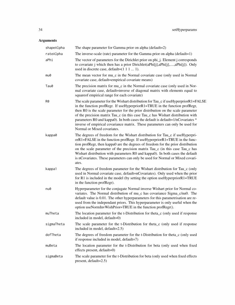
shapeAlpha The shape parameter for Gamma prior on alpha (default=2)

rateAlpha The inverse-scale (rate) parameter for the Gamma prior on alpha (default=1)

aPhi The vector of parameters for the Dirichlet prior on phi_j. Element j correspondsto covariate j which then has a prior Dirichlet(aPhi[j],aPhi[j],....,aPhi[j]). Onlyused in discrete case, default=(1 1 1 ... 1).

mu0 The mean vector for mu_c in the Normal covariate case (only used in Normalcovariate case, default=empirical covariate means)

Tau0 The precision matrix for mu_c in the Normal covariate case (only used in Nor-mal covariate case, default=inverse of diagonal matrix with elements equal tosquareof empirical range for each covariate)

R0 The scale parameter for the Wishart distribution for Tau_c if useHyperpriorR1=FALSEin the function profRegr. If useHyperpriorR1=TRUE in the function profRegr,then R0 is the scale parameter for the prior distribution on the scale parameterof the precision matrix Tau_c (in this case Tau_c has Wishart distribution withparameters R0 and kappa0). In both cases the default is default=1/nCovariates *inverse of empirical covariance matrix. These parameters can only be used forNormal or Mixed covariates.

kappa0 The degrees of freedom for the Wishart distribution for Tau_c if useHyperpri-orR1=FALSE in the function profRegr. If useHyperpriorR1=TRUE in the func-tion profRegr, then kappa0 are the degrees of freedom for the prior distributionon the scale parameter of the precision matrix Tau_c (in this case Tau_c hasWishart distribution with parameters R0 and kappa0). In both cases the defaultis nCovariates. These parameters can only be used for Normal or Mixed covari-ates.

kappa1 The degrees of freedom parameter for the Wishart distribution for Tau_c (onlyused in Normal covariate case, default=nCovariates). Only used when the priorfor R1 is included in the model (by setting the option useHyperpriorR1=TRUEin the function profRegr).

nu0 Hyperparameter for the conjugate Normal inverse Wishart prior for Normal co-variates. The Normal distribution of mu_c has covariance Sigma_c/nu0. Thedefault value is 0.01. The other hyperparameters for this parametrisation are re-used from the independant priors. This hyperparameter is only useful when theoption useNormInvWishPrior=TRUE in the function profRegr().

muTheta The location parameter for the t-Distribution for theta_c (only used if responseincluded in model, default=0)

sigmaTheta The scale parameter for the t-Distribution for theta_c (only used if responseincluded in model, default=2.5)

dofTheta The degrees of freedom parameter for the t-Distribution for theta_c (only usedif response included in model, default=7)

muBeta The location parameter for the t-Distribution for beta (only used when fixedeffects present, default=0)

sigmaBeta The scale parameter for the t-Distribution for beta (only used when fixed effectspresent, default=2.5)

setHyperparams 35

dofBeta The dof parameter for the t-Distribution for beta (only used when fixed effectspresent, default=7)

shapeTauEpsilon

Shape parameter for gamma distribution for prior for precision tau of extra vari-ation errors epsilon (only used if extra variation is used i.e. extraYVar argumentis included, default=5.0)

rateTauEpsilon Inverse-scale (rate) parameter for gamma distribution for prior for precision tauof extra variation errors epsilon (only used if extra variation is used i.e. extraY-Var argument is used, default=0.5)

aRho Parameter for beta distribution for prior on rho in variable selection (default=0.5)

bRho Parameter for beta distribution for prior on rho in variable selection (default=0.5)

atomRho Parameter for the probability for the atom at zero, i.e. the 0.5 probability inw_j distributed Bernoulli(0.5) in the formulation of the sparsity inducing prior(default=0.5). This parameter must be in the interval (0,1], where atomRho=1corresponds to the case where the prior for rho is a Beta(aRho,bRho).

shapeSigmaSqY Shape parameter of inverse-gamma prior for sigma_Y^2 (only used in the Nor-mal response model, default =2.5)

scaleSigmaSqY Scale parameter of inverse-gamma prior for sigma_Y^2 (only used in the Nor-mal response model, default =2.5)

pQuantile Quantile for the yModel=Quantile option (default = 0.5)

rSlice Slice parameter for independent slice sampler such that xi_c = (1-rSlice)*rSlice^cfor c=0,1,2,... (only used for slice independent sampler i.e. sampler=SliceIndependent,default 0.75).

truncationEps Parameter for determining the truncation level of the finite Dirichlet process(only used for truncated sampler i.e. sampler=Truncated

shapeTauCAR Shape parameter for gamma distribution for precision TauCAR of spatial CARterm (only used if a spatial term is included i.e. includeCAR argument is TRUE,default=0.001)

rateTauCAR Inverse-scale (rate) parameter for gamma distribution for precision TauCAR ofspatial CAR term (only used if a spatial term is included i.e. includeCAR argu-ment is TRUE, default=0.001)

shapeNu Shape parameter of Gamma prior for the shape parameter of the Weibull forsurvival response (only used in the Survival response model, default = 2.5)

scaleNu Scale parameter of Gamma prior for the shape parameter of the Weibull forsurvival response (only used in the Survival response model, default = 1)

initAlloc Vector of the initial allocation of the individuals to clusters. This is NULL bydefault, which implies a random start. Useful for starting the MCMC from aspecific partition. Note that if this overwrites the option nClusInit in the functionprofRegr: nClusInit is set equal to the maximum value in initAlloc.

Value

The output of this function is a list with the components defined as above.

36 simBenchmark

Authors




References


Examples

hyp <- setHyperparams(shapeAlpha=3,rateAlpha=2,mu0=c(30,13),R0=3.2*diag(2))

inputs <- generateSampleDataFile(clusSummaryPoissonNormal())runInfoObj<-profRegr(yModel=inputs$yModel,

xModel=inputs$xModel, nSweeps=2, nClusInit=15,nBurn=2, data=inputs$inputData, output="output",covNames = inputs$covNames, outcomeT = inputs$outcomeT,fixedEffectsNames = inputs$fixedEffectNames,hyper=hyp)

simBenchmark Benchmark for simulated examples

Description

This function checks the cluster allocation of profile regression against the generating clusters fora selection of the simulated dataset provided within the package. This can be used to computeconfusion matrices for simulated examples, as shown in the example below.

Usage

simBenchmark(whichModel = "clusSummaryBernoulliDiscrete",nSweeps = 1000, nBurn = 1000, seedProfRegr = 123)

Arguments

whichModel Which simulated dataset this benchmark should be carried out for. At the mo-ment this function works only for these datasets structures provided in the pack-age: "clusSummaryBernoulliNormal","clusSummaryBernoulliDiscreteSmall","clusSummaryCategoricalDiscrete","clusSummaryNormalDiscrete","clusSummaryNormalNormal", "clusSummaryNor-malNormalSpatial", "clusSummaryVarSelectBernoulliDiscrete", "clusSumma-ryBernoulliMixed". These dataset structures can be used by the function gener-ateSampleDataFile to create simulated datasets.

simBenchmark 37

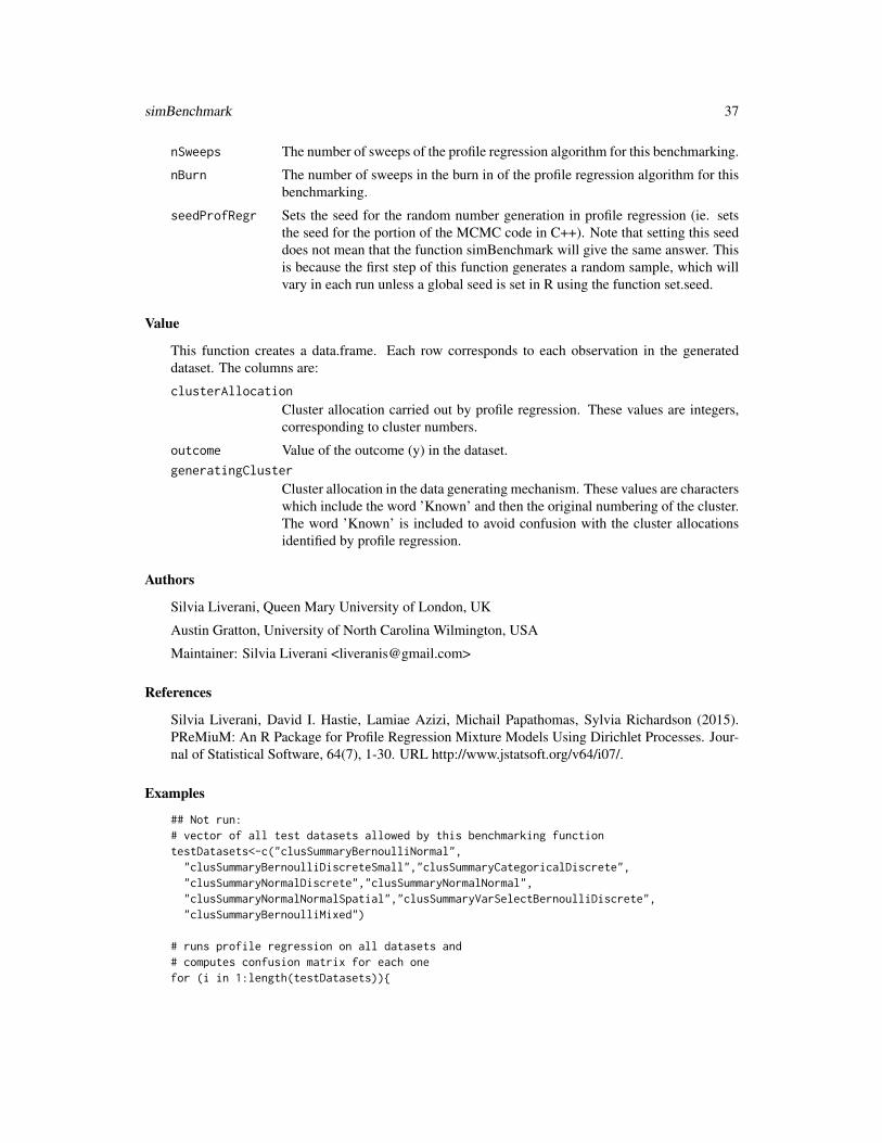
nSweeps The number of sweeps of the profile regression algorithm for this benchmarking.

nBurn The number of sweeps in the burn in of the profile regression algorithm for thisbenchmarking.

seedProfRegr Sets the seed for the random number generation in profile regression (ie. setsthe seed for the portion of the MCMC code in C++). Note that setting this seeddoes not mean that the function simBenchmark will give the same answer. Thisis because the first step of this function generates a random sample, which willvary in each run unless a global seed is set in R using the function set.seed.

Value

This function creates a data.frame. Each row corresponds to each observation in the generateddataset. The columns are:

clusterAllocation

Cluster allocation carried out by profile regression. These values are integers,corresponding to cluster numbers.

outcome Value of the outcome (y) in the dataset.generatingCluster

Cluster allocation in the data generating mechanism. These values are characterswhich include the word ’Known’ and then the original numbering of the cluster.The word ’Known’ is included to avoid confusion with the cluster allocationsidentified by profile regression.

Authors

Silvia Liverani, Queen Mary University of London, UK

Austin Gratton, University of North Carolina Wilmington, USA


References


Examples

## Not run:# vector of all test datasets allowed by this benchmarking functiontestDatasets<-c("clusSummaryBernoulliNormal",

"clusSummaryBernoulliDiscreteSmall","clusSummaryCategoricalDiscrete","clusSummaryNormalDiscrete","clusSummaryNormalNormal","clusSummaryNormalNormalSpatial","clusSummaryVarSelectBernoulliDiscrete","clusSummaryBernoulliMixed")

# runs profile regression on all datasets and# computes confusion matrix for each onefor (i in 1:length(testDatasets)){

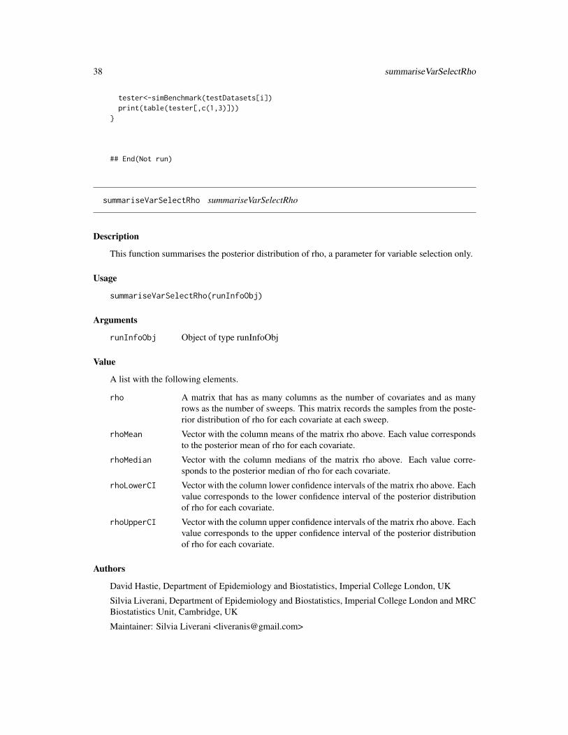
38 summariseVarSelectRho

tester<-simBenchmark(testDatasets[i])print(table(tester[,c(1,3)]))

}

## End(Not run)

summariseVarSelectRho summariseVarSelectRho

Description

This function summarises the posterior distribution of rho, a parameter for variable selection only.

Usage

summariseVarSelectRho(runInfoObj)

Arguments

runInfoObj Object of type runInfoObj

Value

A list with the following elements.

rho A matrix that has as many columns as the number of covariates and as manyrows as the number of sweeps. This matrix records the samples from the poste-rior distribution of rho for each covariate at each sweep.

rhoMean Vector with the column means of the matrix rho above. Each value correspondsto the posterior mean of rho for each covariate.

rhoMedian Vector with the column medians of the matrix rho above. Each value corre-sponds to the posterior median of rho for each covariate.

rhoLowerCI Vector with the column lower confidence intervals of the matrix rho above. Eachvalue corresponds to the lower confidence interval of the posterior distributionof rho for each covariate.

rhoUpperCI Vector with the column upper confidence intervals of the matrix rho above. Eachvalue corresponds to the upper confidence interval of the posterior distributionof rho for each covariate.

Authors




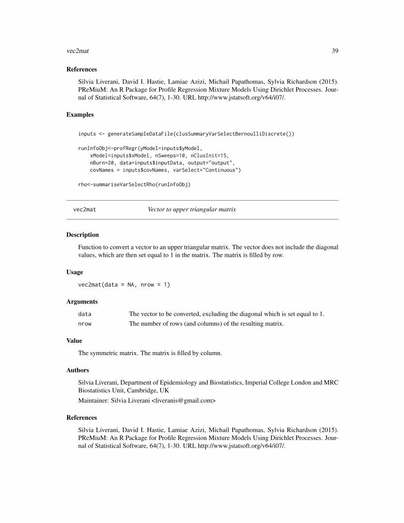
vec2mat 39

References


Examples

inputs <- generateSampleDataFile(clusSummaryVarSelectBernoulliDiscrete())

runInfoObj<-profRegr(yModel=inputs$yModel,xModel=inputs$xModel, nSweeps=10, nClusInit=15,nBurn=20, data=inputs$inputData, output="output",covNames = inputs$covNames, varSelect="Continuous")

rho<-summariseVarSelectRho(runInfoObj)

vec2mat Vector to upper triangular matrix

Description

Function to convert a vector to an upper triangular matrix. The vector does not include the diagonalvalues, which are then set equal to 1 in the matrix. The matrix is filled by row.

Usage

vec2mat(data = NA, nrow = 1)

Arguments

data The vector to be converted, excluding the diagonal which is set equal to 1.nrow The number of rows (and columns) of the resulting matrix.

Value

The symmetric matrix. The matrix is filled by column.

Authors



References


40 vec2mat

Examples

vec2mat(data=c(1,2,3),nrow=3)

Index

∗Topic benchmarksimBenchmark, 36

∗Topic hyperparameterssetHyperparams, 33

∗Topic margModelPosteriormargModelPosterior, 22

∗Topic plotsplotRiskProfile, 24

∗Topic postprocessingcalcAvgRiskAndProfile, 5calcDissimilarityMatrix, 7calcOptimalClustering, 8plotRiskProfile, 24

∗Topic predictions, plotsplotPredictions, 23

∗Topic predictionscalcPredictions, 10

∗Topic profileRegressionprofRegr, 26

∗Topic simulationssimBenchmark, 36

∗Topic simulationclusSummaryBernoulliDiscrete, 13generateSampleDataFile, 17

∗Topic testingsimBenchmark, 36

∗Topic variableSelectionsummariseVarSelectRho, 38

calcAvgRiskAndProfile, 5calcDissimilarityMatrix, 7calcOptimalClustering, 8calcPredictions, 10clusSummaryBernoulliDiscrete, 13clusSummaryBernoulliDiscreteSmall

(clusSummaryBernoulliDiscrete),13

clusSummaryBernoulliMixed(clusSummaryBernoulliDiscrete),13

clusSummaryBernoulliNormal(clusSummaryBernoulliDiscrete),13

clusSummaryBinomialNormal(clusSummaryBernoulliDiscrete),13

clusSummaryCategoricalDiscrete(clusSummaryBernoulliDiscrete),13

clusSummaryNormalDiscrete(clusSummaryBernoulliDiscrete),13

clusSummaryNormalNormal(clusSummaryBernoulliDiscrete),13

clusSummaryNormalNormalSpatial(clusSummaryBernoulliDiscrete),13

clusSummaryPoissonDiscrete(clusSummaryBernoulliDiscrete),13

clusSummaryPoissonNormal(clusSummaryBernoulliDiscrete),13

clusSummaryPoissonNormalSpatial(clusSummaryBernoulliDiscrete),13

clusSummaryQuantileNormal(clusSummaryBernoulliDiscrete),13

clusSummaryVarSelectBernoulliDiscrete(clusSummaryBernoulliDiscrete),13

clusSummaryWeibullDiscrete(clusSummaryBernoulliDiscrete),13

computeRatioOfVariance, 16

generateSampleDataFile, 17globalParsTrace, 18

41

42 INDEX

heatDissMat, 19

is.wholenumber, 20

mapforGeneratedData, 21margModelPosterior, 22

plotPredictions, 23plotRiskProfile, 24PReMiuM (PReMiuM-package), 2PReMiuM-package, 2PReMiuMpackage (PReMiuM-package), 2profRegr, 26

setHyperparams, 33simBenchmark, 36summariseVarSelectRho, 38

vec2mat, 39

Documents

Package ‘PReMiuM’ - The Comprehensive R Archive Network · PReMiuM-package 3 Program to implement Dirichlet Process Bayesian Clustering as described in Liverani et al. 2014. This