Package ‘joineR’March 30, 2012

Version 1.0-1

Date 2012-03-28

Author Pete Philipson, Ines Sousa, Peter Diggle, Paula Williamson,Ruwanthi Kolamunnage-Dona, Robin Henderson

Maintainer Pete Philipson <pete.philipson@northumbria.ac.uk>

Title Joint modelling of repeated measurements and time-to-event data

Description Analysis of repeated measurements and time-to-event datavia random effects joint models. Some plotting functions and the variogram are also included.

Depends R (>= 2.13.0), nlme, MASS, boot, survival, lattice, statmod

License Unlimited

URL http://www.r-project.org

Repository CRAN

Date/Publication 2012-03-30 10:56:43

R topics documented:epileptic . . . . . . . . . . . . . . . . . . . . . . . . . . . . . . . . . . . . . . . . . . . 2heart.valve . . . . . . . . . . . . . . . . . . . . . . . . . . . . . . . . . . . . . . . . . . 3joint . . . . . . . . . . . . . . . . . . . . . . . . . . . . . . . . . . . . . . . . . . . . . 4jointdata . . . . . . . . . . . . . . . . . . . . . . . . . . . . . . . . . . . . . . . . . . . 7jointplot . . . . . . . . . . . . . . . . . . . . . . . . . . . . . . . . . . . . . . . . . . . 8jointSE . . . . . . . . . . . . . . . . . . . . . . . . . . . . . . . . . . . . . . . . . . . 10lines.jointdata . . . . . . . . . . . . . . . . . . . . . . . . . . . . . . . . . . . . . . . . 12liver . . . . . . . . . . . . . . . . . . . . . . . . . . . . . . . . . . . . . . . . . . . . . 13mental . . . . . . . . . . . . . . . . . . . . . . . . . . . . . . . . . . . . . . . . . . . . 14plot.jointdata . . . . . . . . . . . . . . . . . . . . . . . . . . . . . . . . . . . . . . . . 15plot.vargm . . . . . . . . . . . . . . . . . . . . . . . . . . . . . . . . . . . . . . . . . . 16points.jointdata . . . . . . . . . . . . . . . . . . . . . . . . . . . . . . . . . . . . . . . 17sample.jointdata . . . . . . . . . . . . . . . . . . . . . . . . . . . . . . . . . . . . . . . 18

1

2 epileptic

subset.jointdata . . . . . . . . . . . . . . . . . . . . . . . . . . . . . . . . . . . . . . . 19summary.joint . . . . . . . . . . . . . . . . . . . . . . . . . . . . . . . . . . . . . . . . 20summary.jointdata . . . . . . . . . . . . . . . . . . . . . . . . . . . . . . . . . . . . . . 21to.balanced . . . . . . . . . . . . . . . . . . . . . . . . . . . . . . . . . . . . . . . . . 22to.unbalanced . . . . . . . . . . . . . . . . . . . . . . . . . . . . . . . . . . . . . . . . 23UniqueVariables . . . . . . . . . . . . . . . . . . . . . . . . . . . . . . . . . . . . . . . 24variogram . . . . . . . . . . . . . . . . . . . . . . . . . . . . . . . . . . . . . . . . . . 25

Index 27

epileptic Dose calibration of anti-epileptic drugs

Description

The SANAD (Standard and New Antiepileptic Drugs) study (Marson et al, 2007) is a randomisedcontrol trial of standard and new antiepileptic drugs, comparing effects on longer term clinicaloutcomes. The data consists of longitudinal measurements of calibrated dose for the groups ran-domised to a standard drug (CBZ) and a new drug (LTG). The objective of the analysis is to in-vestigate the effect of drug titration on the relative effects of LTG and CBZ on treatment failure(withdrawal of the randomized drug). There are several baseline covariates available, and also dataon the time to withdrawal from randomized drug.

Usage

data(epileptic)

Format

This is a data frame in the unbalanced format, that is, with one row per observation. The dataconsists of columns for patient identifier, time of measurement, calibrated dose, baseline covariates,and survival data. The column names are identified as follows:

• [,1] - id - patient identifier

• [,2] - dose - calibrated dose

• [,3] - time - timing of clinic visit at which dose recorded

• [,4] - with.time - time of drug withdrawal/maximum follow up time

• [,5] - with.status - censoring indicator (1 = withdrawal of randomised drug and 0 = not with-drawn from randomised drug/lost to follow up)

• [,6] - with.status.uae - 1 if withdrawal due to unacceptable adverse effects, 0 otherwise

• [,7] - with.status.isc - 1 if withdrawal due to inadequate seizure control, 0 otherwise

• [,8] - treat - randomized treatment (CBZ or LTG)

• [,9] - age - age of patient at randomization

• [,10] - gender - gender of patient

• [,11] - learn.dis - learning disability

heart.valve 3

Source

SANAD Trial - University of Liverpool

References

Williamson P.R. , Kolamunnage-Dona R, Philipson P, Marson A. G. Joint modelling of longitudinaland competing risks data. Statistics in Medicine, . 27, No. 30. (2008), pp. 6426-6438.

heart.valve Heart Valve surgery

Description

This is longitudinal data on an observational study on detecting effects of different heart valves,differing on type of tissue. The data consists of longitudinal measurements on three different heartfunction outcomes, after surgery occurred. There are several baseline covariates available, and alsosurvival data.

Usage

data(heart.valve)

Format

This is a data frame in the unbalanced format, that is, with one row per observation. The data con-sists in columns for patient identification, time of measurements, longitudinal multiple longitudinalmeasurements, baseline covariates, and survival data. The column names are identified as follows:

• num -number for patient identification

• sex -gender of patient (0=Male and 1=Female)

• age - age of patient at day of surgery

• time - observed time point, with surgery date as the time zero (/years)

• fuyrs - maximum follow up time , with surgery date as the time zero (/years)

• status -censoring indicator (1=died and 0=lost of follow up)

• grad -Gradient, heart function longitudinal outcome

• log.grad -logarithm transformation, with base e, of the Gradient longitudinal outcome

• lvmi -Left Ventricular Mass Index, standardised by mass index, heart function longitudinaloutcome

• log.lvmi -logarithm transformation, with base e, of the lvmi longitudinal outcome

• ef -Ejection Fraction, heart function longitudinal outcome

• bsa -body surface area, baseline covariate

• lvh -Left Ventricular pre-surgery hypertrophy, baseline covariate (0=good and 1=bad)

4 joint

• prenyha -pre-surgery New York Heart Association (NYHA) Classification, baseline covariate(1=I/II and 3=III/IV)

• redo -revision procedure, baseline covariates (0=no and 1=yes)

• size -size of the valve , baseline covariate

• con.cabg -concomitant coronary artery bypass, baseline covariate (0=no and 1=yes)

• creat -creatinine at baseline

• dm -diabetes at baseline (0=no and 1=yes)

• acei -ace inhibitor at baseline (0=no and 1=yes)

• lv -left ventricular pre-surgery function, baseline covariate (1=good and 2=moderate and3=poor)

• emergenc -operative urgency, baseline covariate (0=elective and 1=urgent and 3=emergency)

• hc -high cholesterol , baseline covariate (0=absent and 1=present treated and 2=present un-treated)

• sten.reg.mix -aortic type (1=stenosis and 2=regurgitation and 3=mixed)

• hs -valve type used in the surgery (1=Homograft=human tissue and 0=Stentless=pig tissue)

Source

Eric Lim - Royal Brompton Hospital

References

Lim E., Ali A., Theodorou P., Sousa I., Ashrafian H., Chamageorgakis T., Duncan M., Diggle P.and Pepper J. (2007), A longitudinal study of the profile and predictors of left ventricular massregression after stentless aortic valve replacement, The Annals of Thoracic Surgery 85 (6), June2008, 2026-2029

Examples

data(heart.valve)

joint Fit joint model for survival and longitudinal data measured with error

Description

This generic function fits a joint model with random latent association, building on the formula-tion described in Wulfsohn and Tsiatis (1997) while allowing for the presence of longitudinal andsurvival covariates, and three choices for the latent process. The link between the longitudinal andsurvival processes can be proportional or separate.

joint 5

Usage

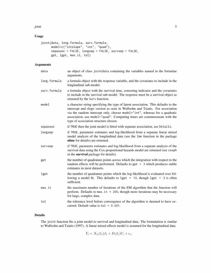
joint(data, long.formula, surv.formula,model=c("intslope", "int", "quad"),sepassoc = FALSE, longsep = FALSE, survsep = FALSE,gpt, lgpt, max.it, tol)

Arguments

data an object of class jointdata containing the variables named in the formulaearguments.

long.formula a formula object with the response variable, and the covariates to include in thelongitudinal sub-model.

surv.formula a formula object with the survival time, censoring indicator and the covariatesto include in the survival sub-model. The response must be a survival object asreturned by the Surv function.

model a character string specifying the type of latent association. This defaults to theintercept and slope version as seen in Wulfsohn and Tsiatis. For associationvia the random intercept only, choose model="int", whereas for a quadraticassociation, use model="quad". Computing times are commensurate with thetype of association structure chosen.

sepassoc if TRUE then the joint model is fitted with separate association, see Details.

longsep if TRUE, parameter estimates and log-likelihood from a separate linear mixedmodel analysis of the longitudinal data (see the lme function in the packagenlme for details) are returned.

survsep if TRUE, parameter estimates and log-likelihood from a separate analysis of thesurvival data using the Cox proportional hazards model are returned (see coxphin the survival package for details).

gpt the number of quadrature points across which the integration with respect to therandom effects will be performed. Defaults to gpt = 3 which produces stableestimates in most datasets.

lgpt the number of quadrature points which the log-likelihood is evaluated over fol-lowing a model fit. This defaults to lgpt = 10, though lgpt = 3 is oftensufficient.

max.it the maximum number of iterations of the EM algorithm that the function willperform. Defaults to max.it = 200, though more iterations may be necessaryfor large, complex data.

tol the tolerance level before convergence of the algorithm is deemed to have oc-curred. Default value is tol = 0.001.

Details

The joint function fits a joint model to survival and longitudinal data. The formulation is similarto Wulfsohn and Tsiatis (1997). A linear mixed effects model is assumed for the longitudinal data

Yi = Xi1(ti)β1 +Di(ti)Ui + εi,

6 joint

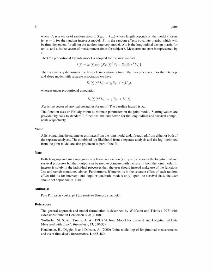
where Ui is a vector of random effects, (U0i, . . . Uqi) whose length depends on the model chosen,ie. q = 1 for the random intercept model. Di is the random effects covariate matrix, which willbe time-dependent for all but the random intercept model. Xi1 is the longitudinal design matrix forunit i, and ti is the vector of measurement times for subject i. Measurement error is represented byεi.

The Cox proportional hazards model is adopted for the survival data,

λ(t) = λ0(t) exp{Xi2(t)Tβ2 +Di(t)(γ

TUi)}.

The parameter γ determines the level of association between the two processes. For the interceptand slope model with separate association we have

Di(t)(γTUi) = γ0U0i + γ1U1it,

whereas under proportional association

Di(t)(γTUi) = γ(U0i + U1it).

Xi2 is the vector of survival covaraites for unit i. The baseline hazard is λ0.

The function uses an EM algorithm to estimate parameters in the joint model. Starting values areprovided by calls to standard R functions lme and coxph for the longitudinal and survival compo-nents respectively.

Value

A list containing the parameter estimates from the joint model and, if required, from either or both ofthe separate analyses. The combined log-likelihood from a separate analysis and the log-likelihoodfrom the joint model are also produced as part of the fit.

Note

Both longsep and survsep ignore any latent association (i.e. γ = 0) between the longitudinal andsurvival processes but their output can be used to compare with the results from the joint model. Ifinterest is solely in the individual processes then the user should instead make use of the functionslme and coxph mentioned above. Furthermore, if interest is in the separate effect of each randomeffect (this is for intercept and slope or quadratic models only) upon the survival data, the usershould set sepassoc = TRUE.

Author(s)

Pete Philipson <pete.philipson@northumbria.ac.uk>

References

The general approach and model formulation is described by Wulfsohn and Tsiatis (1997) withextensions found in Henderson et al (2000).

Wulfsohn, M. S. and Tsiatis, A. A. (1997) ‘A Joint Model for Survival and Longitudinal DataMeasured with Error’. Biometrics, 53, 330-339.

Henderson, R., Diggle, P. and Dobson, A. (2000) ‘Joint modelling of longitudinal measurementsand event time data’. Biostatistics, 1, 465-480.

jointdata 7

See Also

lme, coxph, jointdata, jointplot.

Examples

data(heart.valve)heart.surv <- UniqueVariables(heart.valve,

var.col = c("fuyrs","status"),id.col = "num")

heart.long <- heart.valve[, c("num", "time", "log.lvmi")]heart.cov <- UniqueVariables(heart.valve,

c("age", "hs", "sex"),id.col = "num")

heart.valve.jd <- jointdata(longitudinal = heart.long,baseline = heart.cov,survival = heart.surv,id.col = "num",time.col = "time")

fit <- joint(data = heart.valve.jd,long.formula = log.lvmi ~ 1 + time + hs,surv.formula = Surv(fuyrs,status) ~ hs,model = "intslope")

jointdata Creates an object of class ’jointdata’

Description

This function creates an object of class jointdata. This is an object with information on at leastone of, longitudinal data or survival data. Moreover, it can also have data on baseline covariates.

Usage

jointdata(longitudinal = NA, survival = NA, baseline = NA,id.col = "ID", time.col = NA)

Arguments

longitudinal a data frame or matrix in the unbalanced format (one row per observation), withsubject identification, time of measurements, and longitudinal measurementsand/or time dependent covariates. This must be given if no survival argumentis.

survival a data frame or matrix with survival data for all the subjects. This must be givenif no longitudinal argument is.

baseline a data frame or matrix with baseline covariates, or non-time dependent covari-ates, for the same subjects as in survival and/or longitudinal. This has to bein the balanced format (one row per subject). By default an object of this classdoes not include baseline covariates.

8 jointplot

id.col an element of class character with the name identification of subject. This isto identify the subject identification in the data frames.

time.col an element of class character with the time measurements identification. Thisis to identify the time column in the data frames.

Details

This function creates an object of class jointdata. This is a list with elements used in joint mod-elling, mainly longitudinal and/or survival data. The output has to have at least one of the data sets,longitudinal or survival. However, for joint modelling is necessary to have both data sets. Moreover,a third data frame is possible to be given as input, for the baseline (non-time dependent) covariates.The subject identification and time measurement column names are necessary.

Value

This function returns a list of length six. The first element is the vector of subjects identification.The second is, if exists a data frame of the longitudinal data. The third element of the list is, ifexists a data frame of the survival data. The fourth element of the list is, if exists a data frame onthe baseline covariates. The fifth is, if longitudinal data is given, the column name identification oflongitudinal times. And the sixth and last element of the list is the column name identification ofsubjects.

Author(s)

Ines Sousa (isousa@math.uminho.pt)

Examples

data(heart.valve)heart.surv <- UniqueVariables(heart.valve,

var.col = c("fuyrs", "status"),id.col = "num")

heart.valve.jd <- jointdata(survival = heart.surv,id.col = "num",time.col = "time")

jointplot Joint plot of longitudinal and survival data

Description

This function views the longitudinal profile of each unit with the last longitudinal measurementprior to event-time (censored or not) taken as the end-point, referred to as time zero. In doing so,the shape of the profile prior to event-time can be inspected. This can be done over a user-specifiednumber of time units.

jointplot 9

Usage

jointplot(object, Y.col, Cens.col, lag, split = TRUE, col1, col2,xlab, ylab, gp1lab, gp2lab, smooth,mean.profile = FALSE, mcol1, mcol2)

Arguments

object Name of the jointdata object

Y.col An element of class character identifying the longitudinal response part of thejointdata object.

Cens.col An element of class character identifying the survival status or censoring in-dicator part of the jointdata object.

lag Argument which specifies how many units in time we look back through. De-faults to the maximum observation time across all units.

split TRUE/FALSE argument which allows the profiles of units which ‘fail’ and thosewhich are ‘censored’ to be viewed in separate panels of the same graph. Thisis the default option. Using split = FALSE will plot all profiles overlaid on asingle plot.

col1 argument to choose the colour for the profiles of the ‘censored’ units.

col2 argument to choose the colour for the profiles of the ‘failed’ units.

xlab An element of class character indicating the title for the x-axis.

ylab An element of class character indicating the title for the x-axis.

gp1lab An element of class character for the group corresponding to a censoring in-dicator of zero. Typically, the censored group.

gp2lab An element of class character for the group corresponding to a censoring in-dicator of one. Typically, the group experiencing the event of interest.

smooth the smoother span. This gives the proportion of points in the plot which influ-ence the smooth at each value. Defaults to a value of 2/3. Larger values givemore smoothness. See lowessfor further details.

mean.profile draw mean profiles if TRUE. Only applies to the split = TRUE case.

mcol1 argument to choose the colour for the mean profile of the units with a censoringindicator of zero.

mcol2 argument to choose the colour for the mean profile of the units with a censoringindicator of one.

Details

The function tailors the xyplot function in lattice to produce a representation of joint data withlongitudinal and survival components.

Author(s)

Pete Philipson <pete.philipson@northumbria.ac.uk>

10 jointSE

References

Wulfsohn, M. S. and Tsiatis, A. A. (1997) ‘A Joint Model for Survival and Longitudinal DataMeasured with Error’, Biometrics, 53, 330-339.

See Also

xyplot, joint, jointdata

Examples

data(heart.valve)heart.surv <- UniqueVariables(heart.valve,

var.col = c("fuyrs", "status"),id.col = "num")

heart.long <- heart.valve[,c("num", "time", "log.lvmi")]heart.cov <- UniqueVariables(heart.valve,

c("age", "sex"),id.col = "num")

heart.valve.jd <- jointdata(longitudinal = heart.long,baseline = heart.cov,survival = heart.surv,id.col = "num",time.col = "time")

jointplot(heart.valve.jd, Y.col = "log.lvmi",Cens.col = "status", lag = 5)

jointSE Standard errors via bootstrap for a joint model fit

Description

This function takes a model fit from a joint model and calculates standard errors, with optionalconfidence intervals, for the main longitudinal and survival covariates.

Usage

jointSE(fitted, n.boot, gpt, lgpt, max.it, tol,print.detail = FALSE)

Arguments

fitted A list containing as components the parameter estimates obtained by fitting ajoint model along with the respective formulae for the longitudinal and survivalsub-models and the model chosen, see joint for further details.

n.boot Argument specifying the number of bootstrap samples to use in order to ob-tain the standard error estimates and confidence intervals. Note that at leastn.boot=100 is required in order for the function to return non-zero confidenceintervals.

jointSE 11

gpt the number of quadrature points across which the integration with respect tothe random effects will be performed. Defaults to gpt=3 which produces stableestimates in most datasets.

lgpt the number of quadrature points which the log-likelihood is evaluated over fol-lowing a model fit. This defaults to lgpt = 10, though lgpt = 3 is oftensufficient.

max.it the maximum number of iterations of the EM algorithm that the function willperform. Defaults to max.it = 200, though more iterations may be necessaryfor large, complex data.

tol the tolerance level before convergence of the algorithm is deemed to have oc-curred. Default value is tol = 0.001.

print.detail This argument determines the level of printing that is done during the boot-strapping. If TRUE then the parameter estimates from each bootstrap sample areoutput.

Details

Standard errors and confidence intervals are obtained by repeated fitting of the requisite joint modelto bootstrap samples of the original longitudinal and survival data. It is rare that more than 200bootstrap samples are needed for estimating a standard error. The number of bootstrap samplesneeded for accurate confidence intervals can be as large as 1000.

Author(s)

Ruwanthi Kolamunnage-Dona (Ruwanthi.Kolamunnage-Dona@liverpool.ac.uk) and Pete Philip-son (pete.philipson@northumbria.ac.uk)

References

Wulfsohn, M. S. and Tsiatis, A. A. (1997) ‘A Joint Model for Survival and Longitudinal DataMeasured with Error’. Biometrics, 53, 330-339.

Efron, B. and Tibshirani, J. (1994) ‘An Introduction to the Bootstrap’. Chapman & Hall.

See Also

lme, coxph, joint, jointdata.

Examples

data(heart.valve)heart.surv <- UniqueVariables(heart.valve,

var.col = c("fuyrs", "status"),id.col="num")

heart.long <- heart.valve[, c("num", "time", "log.lvmi")]heart.cov <- UniqueVariables(heart.valve,

c("age", "hs", "sex"),id.col="num")

heart.valve.jd <- jointdata(longitudinal = heart.long,baseline = heart.cov,

12 lines.jointdata

survival = heart.surv,id.col = "num",time.col = "time")

fit <- joint(heart.valve.jd,long.formula = log.lvmi ~ 1 + time + hs,surv.formula = Surv(fuyrs,status) ~ hs,model = "int")

jointSE(fitted = fit, n.boot = 10)

lines.jointdata Add lines to an existing jointdata plot

Description

Add lines to an existing plot of an object of Class ’jointdata’, for a longitudinal variable. It ispossible to plot all the subjects in the data set, or just a selected subset. See subset.jointdata

Usage

## S3 method for class ’jointdata’lines(x, Y.col, ...)

Arguments

x object of class ’jointdata’

Y.col column number, or column name, of longitudinal variable to be plotted

... other graphical arguments

Value

A graphical device with a plot for longitudinal data. Other functions are useful to be used with thisas plot and points

Author(s)

Ines Sousa (isousa@math.uminho.pt)

Examples

data(heart.valve)heart.surv <- UniqueVariables(heart.valve, var.col = c("fuyrs", "status"),

id.col = "num")heart.long <- heart.valve[, c(1, 4, 5, 7, 8, 9, 10, 11)]heart.jd <- jointdata(longitudinal = heart.long,

survival = heart.surv, id.col = "num", time.col = "time")# Randomly select a pair of subjects to plot profiles oftake <- sample(1 : max(heart.jd$survival$num), 2)heart.jd.1 <- subset(heart.jd, take[1])heart.jd.2 <- subset(heart.jd, take[2])

liver 13

plot(heart.jd.1, Y.col = 4)lines(heart.jd.2, Y.col = 4, lty = 2)

liver Liver cirrhosis longitudinal data

Description

This dataset gives the longitudinal observations of prothrombin index, a measure of liver function,for patients from a controlled trial into prednisone treatment of liver cirrhosis. Time-to-event infor-mation in the form of the event time and associated censoring indicator are also recorded along witha solitary baseline covariate - the allocated treatment arm in this instance. The data are taken fromAndersen et al (1993, p. 19) and were analysed in Henderson, Diggle and Dobson (2002). This isa subset of the full data where a number of variables were recorded both at entry and during thecourse of the trial.

Usage

data(liver)

Format

A data frame in the unbalanced format with longitudinal observations from 488 subjects. Thecolumn form of the data is subject identifier, prothrombin index measurement, time of prothrombinindex measurement, treatment indicator and then the survival data. The column names are detailedbelow:

• id -number for patient identification

• prothrombin -prothrombin index measurement (?units)

• time -time of prothrombin index measurement

• treatment -patient treatment indicator (0 = placebo, 1 = prednisone)

• survival -patient survival time (in years)

• cens -censoring indicator (1 = died and 0 = censored)

Source

Andersen, P. K., Borgan O., Gill, R. D. and Kieding, N. (1993). Statistical Models Based onCounting Processes. New York: Springer.

References

Andersen, P. K., Borgan O., Gill, R. D. and Kieding, N. (1993). Statistical Models Based onCounting Processes. New York: Springer.

Henderson, R., Diggle, P. and Dobson, A. (2002). Identification and efficacy of longitudinal markersfor survival. Biostatistics 3, 33-50.

14 mental

Examples

data(liver)

mental Mental Health Trial Data

Description

The data is obtained from a trial in which chronically ill mental health patients were randomisedacross two treatments: placebo and an active drug. A questionnaire instrument was used to assesseach patient’s mental state at weeks 0, 1, 2, 4, 6 and 8 post-randomisation, a high recorded scoreimplying a severe condition. Some of the 100 patients dropped out of the study for reasons that werethought to be related to their mental state, and therefore potentially informative; others dropped outfor reasons unrelated to their mental state.

Usage

data(mental)

Format

A balanced data set with respect to the times at which observations recorded. The data consists ofthe following variables on each patient:

• [,1] - id - patient identifier (1,2,...,100)

• [,2] - Y.t0 - mental state assessment in week 0 (coded NA if missing)

• [,3] - Y.t1 - mental state assessment in week 1

• [,4] - Y.t2 - mental state assessment in week 2

• [,5] - Y.t4 - mental state assessment in week 4

• [,6] - Y.t6 - mental state assessment in week 6

• [,7] - Y.t8 - mental state assessment in week 8

• [,8] - treat - treatment allocation (0=placebo; 1=active drug)

• [,9] - n.obs - number of non-missing mental state assessments

• [,10] - event.time - imputed dropout time in weeks (coded 8.002 for completers)

• [,11] - status - censoring indicator (0=completer or non-informative dropout, 1=potentiallyinformative dropout)

plot.jointdata 15

plot.jointdata Plot longitudinal data

Description

Plot longitudinal data of an object of class jointdata, for a longitudinal variable. It is possible toplot all the subjects in the data set, or just a selected subset. See subset.jointdata.

Usage

## S3 method for class ’jointdata’plot(x, Y.col, type, xlab, xlim, ylim, main, pty, ...)

Arguments

x object of class jointdata

Y.col column number, or column name, of longitudinal variable to be plotted. Defaultsto Y.col = NA, plotting all longitudinal variables

type the type of line to be plotted, see plot for further details.

xlab a title for the x-axis, see title.

xlim, ylim numeric vectors of length 2, giving the x and y coordinates ranges, see plot.windowfor further details.

main an overall title for the plot: see title.

pty A character specifying the type of plot region to be used, see par for details.

... other graphical arguments (see plot)

Value

A graphical device with a plot for longitudinal data. Other functions are useful to be used with thisas lines and points

Author(s)

Ines Sousa (isousa@math.uminho.pt)

Examples

data(heart.valve)heart.surv <- UniqueVariables(heart.valve, var.col = c("fuyrs", "status"),

id.col = "num")heart.long <- heart.valve[, c(1, 4, 5, 7, 8, 9, 10, 11)]heart.jd <- jointdata(longitudinal = heart.long,

survival = heart.surv, id.col = "num", time.col = "time")plot(heart.jd, Y.col = "grad", col = "grey")

16 plot.vargm

plot.vargm Plots the empirical variogram for longitudinal data

Description

Plots the empirical variogram for observed measurements, of an object of class ’vargm’, obtainedby using function variogram.

Usage

## S3 method for class ’vargm’plot(x, smooth = FALSE, bdw = NULL, follow.time = NULL, points = TRUE, ...)

Arguments

x object of class vargm obtained by using function variogram

smooth Logical value to use a non-parametric estimator to calculate the variogram of all$v_ijk$. The default is FALSE, as it uses time averages

bdw bandwidth to use in the time averages. The default is NULL, because this iscalculated automatically.

follow.time the interval of time we want to construct the variogram for. When NULL this isthe maximum of the data

points Logical value if the points $v_ijk$ should be plotted

... other graphical options as in par

Value

The function returns a graphical device with the plot of empirical variogram

Author(s)

Ines Sousa (isousa@math.uminho.pt)

Examples

data(mental)mental.unbalanced <- to.unbalanced(mental, id.col = 1,

times = c(0,1,2,4,6,8),Y.col = 2:7,other.col = c(8,10,11))

names(mental.unbalanced)[3] <- "Y"vgm <- variogram(indv = mental.unbalanced[, 1],

time = mental.unbalanced[, 2],Y = mental.unbalanced[, 3])

plot(vgm, ylim = c(0, 500))

points.jointdata 17

points.jointdata Add points to an existing jointdata plot

Description

Add points to an existing plot of an object of class jointdata, for a longitudinal variable. It ispossible plot all the subjects in the data set, or just a selected subset. See subset.jointdata

Usage

## S3 method for class ’jointdata’points(x, Y.col, ...)

Arguments

x object of class jointdata

Y.col column number, or column name, of longitudinal variable to be plotted

... other graphical arguments

Value

A graphical device with a plot for longitudinal data. Other functions are useful to be used with thisas plot and lines

Author(s)

Ines Sousa (isousa@math.uminho.pt)

Examples

data(heart.valve)heart.surv <- UniqueVariables(heart.valve, var.col = c("fuyrs", "status"),

id.col = "num")heart.long <- heart.valve[, c(1, 4, 5, 7, 8, 9, 10, 11)]heart.jd <- jointdata(longitudinal = heart.long,

survival = heart.surv, id.col = "num", time.col = "time")# Randomly select a pair of subjects to plot profiles oftake <- sample(1 : max(heart.jd$survival$num), 2)heart.jd.1 <- subset(heart.jd, take[1])heart.jd.2 <- subset(heart.jd, take[2])plot(heart.jd.1, Y.col = "grad", type = "p")points(heart.jd.2, Y.col = "grad", col = "blue", pch = 20)

18 sample.jointdata

sample.jointdata Sample from a jointdata object

Description

Generic function used to sampling a subset of data from an object of class jointdata, with aspecific size of number of subjects.

Usage

sample.jointdata(object, size, replace = FALSE)

Arguments

object an object of class jointdata

size number of subjects to include in the sampled subset

replace should sampling be with replacement?

Value

The function returns an object of class jointdata, with data only on the subjects sampled.

Author(s)

Ines Sousa (isousa@math.uminho.pt)

See Also

sample, jointdata, UniqueVariables.

Examples

data(heart.valve)heart.surv <- UniqueVariables(heart.valve,

var.col=c("fuyrs", "status"),id.col = "num")

heart.valve.jd <- jointdata(survival = heart.surv,id.col = "num",time.col = "time")

sample.jointdata(heart.valve.jd, size = 10)

subset.jointdata 19

subset.jointdata Subsetting object of class ’jointdata’

Description

Returns an object of class jointdata which is a subset of an original object of class jointdata.

Usage

## S3 method for class ’jointdata’subset(x, subj.subset, ...)

Arguments

x an object of class jointdata

subj.subset vector of subject identifiers, to include in the data subset. This must be a uniquevector of patient identifiers.

... further arguments to be passed to or from other methods.

Value

The function returns an object of class jointdata, with data only on a subset of subjects.

Author(s)

Ines Sousa (isousa@math.uminho.pt)

Examples

data(heart.valve)heart.surv <- UniqueVariables(heart.valve, var.col = c("fuyrs", "status"),

id.col = "num")heart.long <- heart.valve[, c(1, 4, 5, 7, 8, 9, 10, 11)]heart.jd <- jointdata(longitudinal = heart.long,

survival = heart.surv, id.col = "num", time.col = "time")take <- heart.jd$survival$num[heart.jd$survival$status == 0]heart.jd.cens <- subset(heart.jd, take)

20 summary.joint

summary.joint Summarise a random effects joint model fit

Description

Generic function used to produce summary information from a fitted random effects joint model asrepresented by object of class joint.

Usage

## S3 method for class ’joint’summary(object, variance, ...)

Arguments

object an object inheriting from class joint representing a fitted random effects jointmodel.

variance should the variance components be output as variances or standard deviations?Defaults to variance = TRUE.

... further arguments for the summary

Value

an object inheriting from class summary.joint with all components included in object (see jointfor a full description of the components) plus the following components:

nobs the total number of (typically longitudinal) observations (i.e. rows in an unbal-anced data set).

ngrps the number of groups in the analysed dataset, often individual subjects.

Author(s)

Pete Philipson (pete.philipson@northmbria.ac.uk)

Examples

data(heart.valve)heart.surv <- UniqueVariables(heart.valve,

var.col=c("fuyrs","status"),id.col="num")

heart.long <- heart.valve[, c("num", "time", "log.lvmi")]heart.cov <- UniqueVariables(heart.valve,

c("age", "hs", "sex"),id.col = "num")

heart.valve.jd <- jointdata(longitudinal = heart.long,baseline = heart.cov,survival = heart.surv,id.col = "num",

summary.jointdata 21

time.col = "time")fit <- joint(data = heart.valve.jd,

long.formula = log.lvmi ~ 1 + time + hs,surv.formula = Surv(fuyrs,status) ~ hs,model = "intslope")

summary(fit)

summary.jointdata Summarise a jointdata object

Description

Generic function used to produce summaries of objects of class jointdata

Usage

## S3 method for class ’jointdata’summary(object, ...)

Arguments

object an object of class jointdata

... further arguments for the summary

Value

The function returns a list with five elements. Each summarises each element of the jointdataobject.

subjects Gives the number of subjects in the data set.

longitudinal If longitudinal data is available, it gives the names and class, of the longitudinalvariables.

survival If survival data is available, it gives the number of subjects with failure andcensored survival times.

baseline If baseline covariates is available, it gives the names and class, of the baselinecovariates.

times If longitudinal data is available, it gives the unique longitudinal time measure-ments, if it is a balanced study. In case of unbalanced study , it will only state itis an unbalanced study.

Author(s)

Ines Sousa (isousa@math.uminho.pt)

See Also

jointdata, UniqueVariables.

22 to.balanced

Examples

data(heart.valve)heart.surv <- UniqueVariables(heart.valve,

var.col = c("fuyrs", "status"),id.col = "num")

heart.valve.jd <- jointdata(survival = heart.surv,id.col = "num",time.col = "time")

summary(heart.valve.jd)

to.balanced Transform data to the longitudinal balanced format

Description

Transforms a longitudinal data set in the unbalanced format TO the balanced format

Usage

to.balanced(data, id.col, time.col, Y.col, other.col = NA)

Arguments

data a data frame with longitudinal data in the unbalanced format. That is, in theformat of ’one row per observation’.

id.col a column number, or column name, in the data frame data, where the patientidentifier is located.

time.col a column number, or column name, in the data frame data, where the timemeasurements are.

Y.col a vector of column numbers, or column names, of longitudinal variables, and/ortime dependent covariates in the data frame data.

other.col a vector of column numbers, or column names, of baseline covariates, and/orother subject level data, as for example, survival data. Default does not includeother.col.

Value

The function returns a data frame with longitudinal data in the balanced format. The balanced for-mat is considered in this context as the format where each row has data on each subject. Notice thatin this format we will have multiple columns for the same longitudinal variable, each correspondingto the variable observed at each time point.

Author(s)

Ines Sousa (isousa@math.uminho.pt)

to.unbalanced 23

See Also

to.unbalanced.

Examples

simul <- data.frame(num = 1:10, Y1.1 = rnorm(10), Y1.2 = rnorm(10),Y2.1 = rnorm(10),Y2.2 = rnorm(10), age = rnorm(10))

simul <- to.unbalanced(simul, id.col = 1, times = c(1,2),Y.col = 2:5, other.col = 6)

simul<-to.balanced(simul, id.col = "num", time.col = "time",Y.col = c("Y1.1","Y2.1"), other.col = "age")

to.unbalanced Transform data to the longitudinal unbalanced format

Description

Transforms a longitudinal data set in the balanced format TO the unbalanced format

Usage

to.unbalanced(data, id.col, times, Y.col, other.col = NA)

Arguments

data a data frame with longitudinal data in the balanced format. That is, in the formatof ’one row per subject’.

id.col a column number, or column name, in the data frame data, where the patientidentifications is.

times a vector with the unique time points where the patients are observed. This is thestudy design time points in a balanced data set.

Y.col a vector of column numbers, or column names, of longitudinal variables, and/ortime dependent covariates in the data frame data.

other.col a vector of column numbers, or column names, of baseline covariates, and/orother subject level data, as for example, survival data. Default does not includeother.col.

Value

The function returns a data frame with longitudinal data in the unbalanced format. The unbal-anced format is considered in this context as the format where each row has data on each subjectobservation.

Author(s)

Ines Sousa (isousa@uminho.pt)

24 UniqueVariables

See Also

to.balanced.

Examples

simul <- data.frame(num = 1:10,Y1.1 = rnorm(10),Y1.2 = rnorm(10),Y2.1 = rnorm(10),Y2.2 = rnorm(10), age = rnorm(10))

to.unbalanced(simul, id.col = 1, times = c(1,2), Y.col = 2:5,other.col = 6)

UniqueVariables Extracts the unique non-time dependent variables per patient, from anunbalanced data set

Description

This function extracts a set of unique variables within a patient, returning a data frame with columns,patient identification and variables selected. Each row corresponds to the data for each individual.

Usage

UniqueVariables(data,var.col,id.col="ID")

Arguments

data data frame, or matrix, with at least a column of patient identification and a co-variate column

var.col vector of column names or column numbers, of the variables (non-time depen-dent). Cannot have mix of numbers and column names.

id.col column name or column number of the patient identification

Details

This function can be used, when longitudinal data is in the unbalanced format, and it is necessary,for example, to extract the set of unique baseline covariates, or any non-time dependent variables,that in the unbalanced format, are repeated for each observation row. Also, if the original data framehas survival data, this can also be used to extract the survival information from the original data set.

Value

The function returns a data frame with patient identification and covariates selected. Each rowcorresponds to the data for each individual. Note that, this can be only used for non-time dependentcovariates. If extracting unique time dependent covariates, the function gives an error, because itcan’t select what is the unique covariate.

Author(s)

Ines Sousa (isousa@math..pt)

variogram 25

Examples

data(heart.valve)heart.cov <- UniqueVariables(heart.valve,

c(2, 3, 5, 6, 12:25),id.col = "num")

variogram Empirical variogram for longitudinal data

Description

Calculates the variogram for observed measurements, with two components, the total variability inthe data, and the variogram for all time lags in all individuals.

Usage

variogram(indv, time, Y)

Arguments

indv vector of individual identification, as in the longitudinal data, repeated for eachtime point

time vector of observation time, as in the longitudinal data

Y vector of observed measurements. This can be a vector of longitudinal data, orresiduals after fitting a model for the mean response

Details

The empirical variogram in this function is calculated from observed half-squared-differences be-tween pairs of measurements, $$v_ijk = 0.5 * (r_ij-r_ik)^2$$ and the corresponding time differ-ences $$u_ijk=t_ij-t_ik$$. The variogram is plotted for averages of each time lag for the $v_ijk$for all $i$

Value

The function returns a list with two elements. The first svar is a matrix with columns for all values$(u_ijk,v_ijk)$, and the second sigma2 is the total variability in the data. This is an object of classvargm

Note

There is a function plot.vargm which should be used to plot the empirical variogram.

Author(s)

Ines Sousa (isousa@math.uminho.pt)

26 variogram

Examples

data(mental)mental.unbalanced <- to.unbalanced(mental, id.col = 1,

times = c(0,1,2,4,6,8),Y.col = 2:7,other.col = c(8,10,11))

names(mental.unbalanced)[3] <- "Y"vgm <- variogram(indv = mental.unbalanced[, 1],

time = mental.unbalanced[, 2],Y = mental.unbalanced[, 3])

Index

∗Topic balancedto.balanced, 22to.unbalanced, 23

∗Topic datasetsepileptic, 2heart.valve, 3liver, 13mental, 14

∗Topic jointdatasubset.jointdata, 19

∗Topic lines, longitudinal, jointdatalines.jointdata, 12

∗Topic modelsjoint, 4jointplot, 8jointSE, 10summary.joint, 20

∗Topic plot, longitudinal, jointdataplot.jointdata, 15

∗Topic points, longitudinal, jointdatapoints.jointdata, 17

∗Topic survivaljoint, 4jointdata, 7jointplot, 8jointSE, 10sample.jointdata, 18summary.jointdata, 21UniqueVariables, 24

∗Topic variogramplot.vargm, 16variogram, 25

epileptic, 2

heart.valve, 3

joint, 4jointdata, 7jointplot, 8

jointSE, 10

lines, 15, 17lines.jointdata, 12liver, 13

mental, 14

plot, 12, 17plot.jointdata, 15plot.vargm, 16, 25points, 12, 15points.jointdata, 17

sample.jointdata, 18subset.jointdata, 12, 15, 17, 19summary.joint, 20summary.jointdata, 21

to.balanced, 22to.unbalanced, 23

UniqueVariables, 24

variogram, 16, 25

27