Package ‘FD’ ‘FD’ February 19, 2015 Type Package Title Measuring functional diversity (FD) from multiple traits, and other tools for functional ecology

Package ‘FD’February 19, 2015

Type PackageTitle Measuring functional diversity (FD) from multiple traits, and

other tools for functional ecologyVersion 1.0-12Date 2014-19-08Author Etienne Laliberté, Pierre Legendre, Bill ShipleyMaintainer Etienne Laliberté <[email protected]>

Description FD is a package to compute different multidimensional FD indices. It implements a dis-tance-based framework to measure FD that allows any number and type of func-tional traits, and can also consider species relative abundances. It also contains other use-ful tools for functional ecology.

License GPL-2LazyLoad yesLazyData yesDepends ade4, ape, geometry, veganEncoding latin1NeedsCompilation yesRepository CRANDate/Publication 2014-08-19 13:42:17

R topics documented:FD-package . . . . . . . . . . . . . . . . . . . . . . . . . . . . . . . . . . . . . . . . . 2dbFD . . . . . . . . . . . . . . . . . . . . . . . . . . . . . . . . . . . . . . . . . . . . 3dummy . . . . . . . . . . . . . . . . . . . . . . . . . . . . . . . . . . . . . . . . . . . 10fdisp . . . . . . . . . . . . . . . . . . . . . . . . . . . . . . . . . . . . . . . . . . . . . 10functcomp . . . . . . . . . . . . . . . . . . . . . . . . . . . . . . . . . . . . . . . . . . 12gowdis . . . . . . . . . . . . . . . . . . . . . . . . . . . . . . . . . . . . . . . . . . . . 14mahaldis . . . . . . . . . . . . . . . . . . . . . . . . . . . . . . . . . . . . . . . . . . . 17maxent . . . . . . . . . . . . . . . . . . . . . . . . . . . . . . . . . . . . . . . . . . . . 18maxent.test . . . . . . . . . . . . . . . . . . . . . . . . . . . . . . . . . . . . . . . . . 22simul.dbFD . . . . . . . . . . . . . . . . . . . . . . . . . . . . . . . . . . . . . . . . . 24tussock . . . . . . . . . . . . . . . . . . . . . . . . . . . . . . . . . . . . . . . . . . . 26

1

2 FD-package

Index 28

FD-package Measuring Functional Diversity from Multiple Traits, and Other Toolsfor Functional Ecology

Description

FD is a package to compute different multidimensional functional diversity (FD) indices. It imple-ments a distance-based framework to measure FD that allows any number and type of functionaltraits, and can also consider species relative abundances. It also contains other tools for functionalecologists (e.g. maxent).

Details

Package: FDType: PackageVersion: 1.0-12Date: 2014-08-19License: GPL-2LazyLoad: yesLazyData: yes

FD computes different multidimensional FD indices. To compute FD indices, a species-by-trait(s)matrix is required (or at least a species-by-species distance matrix). gowdis computes the Gowerdissimilarity from different trait types (continuous, ordinal, nominal, or binary), and tolerates NAs. Itcan treat ordinal variables as described by Podani (1999), and can handle asymetric binary variablesand variable weights. gowdis is called by dbFD, the main function of FD.

dbFD uses principal coordinates analysis (PCoA) to return PCoA axes, which are then used as ‘traits’to compute FD. dbFD computes several multidimensional FD indices, including the three indicesof Villéger et al. (2008): functional richness (FRic), functional evenness (FEve), and functionaldivergence (FDiv). It also computes functional dispersion (FDis) (Laliberté and Legendre 2010),Rao’s quadratic entropy (Q) (Botta-Dukát 2005), a posteriori functional group richness (FGR), andthe community-level weighted means of trait values (CWM), an index of functional composition.Some of these indices can be weighted by species abundances. dbFD includes several options forflexibility.

Author(s)

Etienne Laliberté, Pierre Legendre and Bill Shipley

Maintainer: Etienne Laliberté <[email protected]> http://www.elaliberte.info

References

Botta-Dukát, Z. (2005) Rao’s quadratic entropy as a measure of functional diversity based on mul-tiple traits. Journal of Vegetation Science 16:533-540.

http://www.elaliberte.info

dbFD 3

Laliberté, E. and P. Legendre (2010) A distance-based framework for measuring functional diversityfrom multiple traits. Ecology 91:299-305.

Podani, J. (1999) Extending Gower’s general coefficient of similarity to ordinal characters. Taxon48:331-340.

Villéger, S., N. W. H. Mason and D. Mouillot (2008) New multidimensional functional diversityindices for a multifaceted framework in functional ecology. Ecology 89:2290-2301.

Examples

# examples with a dummy dataset

ex1 <- gowdis(dummy$trait)ex1

ex2 <- functcomp(dummy$trait, dummy$abun)ex2

ex3 <- dbFD(dummy$trait, dummy$abun)ex3

# examples with real data from New Zealand short-tussock grasslands# these examples may take a few seconds to a few minutes each to run

ex4 <- gowdis(tussock$trait)

ex5 <- functcomp(tussock$trait, tussock$abun)

# 'lingoes' correction used because 'sqrt' does not work in that caseex6 <- dbFD(tussock$trait, tussock$abun, corr = "lingoes")

## Not run:# ward clustering to compute FGR, cailliez correctionex7 <- dbFD(tussock$trait, tussock$abun, corr = "cailliez",calc.FGR = TRUE, clust.type = "ward")# choose 'g' for number of groups# 6 groups seems to make good ecological senseex7

# however, calinksi criterion in 'kmeans' suggests# that 6 groups may not be optimalex8 <- dbFD(tussock$trait, tussock$abun, corr = "cailliez",calc.FGR = TRUE, clust.type = "kmeans", km.sup.gr = 10)

## End(Not run)

dbFD Distance-Based Functional Diversity Indices

4 dbFD

Description

dbFD implements a flexible distance-based framework to compute multidimensional functional di-versity (FD) indices. dbFD returns the three FD indices of Villéger et al. (2008): functional richness(FRic), functional evenness (FEve), and functional divergence (FDiv), as well functional dispersion(FDis; Laliberté and Legendre 2010), Rao’s quadratic entropy (Q) (Botta-Dukát 2005), a posteriorifunctional group richness (FGR) (Petchey and Gaston 2006), and the community-level weightedmeans of trait values (CWM; e.g. Lavorel et al. 2008). Some of these FD indices consider speciesabundances. dbFD includes several options for flexibility.

Usage

dbFD(x, a, w, w.abun = TRUE, stand.x = TRUE,ord = c("podani", "metric"), asym.bin = NULL,corr = c("sqrt", "cailliez", "lingoes", "none"),calc.FRic = TRUE, m = "max", stand.FRic = FALSE,scale.RaoQ = FALSE, calc.FGR = FALSE, clust.type = "ward",km.inf.gr = 2, km.sup.gr = nrow(x) - 1, km.iter = 100,km.crit = c("calinski", "ssi"), calc.CWM = TRUE,CWM.type = c("dom", "all"), calc.FDiv = TRUE, dist.bin = 2,print.pco = FALSE, messages = TRUE)

Arguments

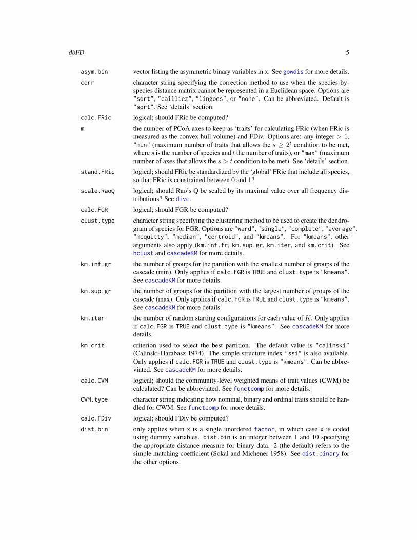
x matrix or data frame of functional traits. Traits can be numeric, ordered, orfactor. Binary traits should be numeric and only contain 0 and 1. charactertraits will be converted to factor. NAs are tolerated.x can also be a species-by-species distance matrix of class dist, in which caseNAs are not allowed.When there is only one trait, x can be also be a numeric vector, an orderedfactor, or a unordered factor.In all cases, species labels are required. .

a matrix containing the abundances of the species in x (or presence-absence, i.e.0 or 1). Rows are sites and species are columns. Can be missing, in which casedbFD assumes that there is only one community with equal abundances of allspecies. NAs will be replaced by 0. The number of species (columns) in a mustmatch the number of species (rows) in x. In addition, the species labels in a andx must be identical and in the same order.

w vector listing the weights for the traits in x. Can be missing, in which case alltraits have equal weights.

w.abun logical; should FDis, Rao’s Q, FEve, FDiv, and CWM be weighted by the rela-tive abundances of the species?

stand.x logical; if all traits are numeric, should they be standardized to mean 0 and unitvariance? If not all traits are numeric, Gower’s (1971) standardization by therange is automatically used; see gowdis for more details.

ord character string specifying the method to be used for ordinal traits (i.e. ordered)."podani" refers to Eqs. 2a-b of Podani (1999), while "metric" refers to his Eq.3. Can be abbreviated. See gowdis for more details.

dbFD 5

asym.bin vector listing the asymmetric binary variables in x. See gowdis for more details.

corr character string specifying the correction method to use when the species-by-species distance matrix cannot be represented in a Euclidean space. Options are"sqrt", "cailliez", "lingoes", or "none". Can be abbreviated. Default is"sqrt". See ‘details’ section.

calc.FRic logical; should FRic be computed?

m the number of PCoA axes to keep as ‘traits’ for calculating FRic (when FRic ismeasured as the convex hull volume) and FDiv. Options are: any integer > 1,"min" (maximum number of traits that allows the s ≥ 2t condition to be met,where s is the number of species and t the number of traits), or "max" (maximumnumber of axes that allows the s > t condition to be met). See ‘details’ section.

stand.FRic logical; should FRic be standardized by the ‘global’ FRic that include all species,so that FRic is constrained between 0 and 1?

scale.RaoQ logical; should Rao’s Q be scaled by its maximal value over all frequency dis-tributions? See divc.

calc.FGR logical; should FGR be computed?

clust.type character string specifying the clustering method to be used to create the dendro-gram of species for FGR. Options are "ward", "single", "complete", "average","mcquitty", "median", "centroid", and "kmeans". For "kmeans", otherarguments also apply (km.inf.fr, km.sup.gr, km.iter, and km.crit). Seehclust and cascadeKM for more details.

km.inf.gr the number of groups for the partition with the smallest number of groups of thecascade (min). Only applies if calc.FGR is TRUE and clust.type is "kmeans".See cascadeKM for more details.

km.sup.gr the number of groups for the partition with the largest number of groups of thecascade (max). Only applies if calc.FGR is TRUE and clust.type is "kmeans".See cascadeKM for more details.

km.iter the number of random starting configurations for each value of K. Only appliesif calc.FGR is TRUE and clust.type is "kmeans". See cascadeKM for moredetails.

km.crit criterion used to select the best partition. The default value is "calinski"(Calinski-Harabasz 1974). The simple structure index "ssi" is also available.Only applies if calc.FGR is TRUE and clust.type is "kmeans". Can be abbre-viated. See cascadeKM for more details.

calc.CWM logical; should the community-level weighted means of trait values (CWM) becalculated? Can be abbreviated. See functcomp for more details.

CWM.type character string indicating how nominal, binary and ordinal traits should be han-dled for CWM. See functcomp for more details.

calc.FDiv logical; should FDiv be computed?

dist.bin only applies when x is a single unordered factor, in which case x is codedusing dummy variables. dist.bin is an integer between 1 and 10 specifyingthe appropriate distance measure for binary data. 2 (the default) refers to thesimple matching coefficient (Sokal and Michener 1958). See dist.binary forthe other options.

6 dbFD

print.pco logical; should the eigenvalues and PCoA axes be returned?

messages logical; should warning messages be printed in the console?

Details

Typical usage is

dbFD(x, a, ...)

If x is a matrix or a data frame that contains only continuous traits, no NAs, and that no weightsare specified (i.e. w is missing), a species-species Euclidean distance matrix is computed via dist.Otherwise, a Gower dissimilarity matrix is computed via gowdis. If x is a distance matrix, it istaken as is.

When x is a single trait, species with NAs are first excluded to avoid NAs in the distance matrix. Ifx is a single continuous trait (i.e. of class numeric), a species-species Euclidean distance matrix iscomputed via dist. If x is a single ordinal trait (i.e. of class ordered), gowdis is used and argumentord applies. If x is a single nominal trait (i.e. an unordered factor), the trait is converted to dummyvariables and a distance matrix is computed via dist.binary, following argument dist.bin.

Once the species-species distance matrix is obtained, dbFD checks whether it is Euclidean. Thisis done via is.euclid. PCoA axes corresponding to negative eigenvalues are imaginary axes thatcannot be represented in a Euclidean space, but simply ignoring these axes would lead to biasedestimations of FD. Hence in dbFD one of four correction methods are used, following argumentcorr. "sqrt" simply takes the square root of the distances. However, this approach does not alwayswork for all coefficients, in which case dbFD will stop and tell the user to select another correctionmethod. "cailliez" refers to the approach described by Cailliez (1983) and is implemented viacailliez. "lingoes" refers to the approach described by Lingoes (1971) and is implemented vialingoes. "none" creates a distance matrix with only the positive eigenvalues of the Euclideanrepresentation via quasieuclid. See Legendre and Legendre (1998) and Legendre and Anderson(1999) for more details on these corrections.

Principal coordinates analysis (PCoA) is then performed (via dudi.pco) on the corrected species-species distance matrix. The resulting PCoA axes are used as the new ‘traits’ to compute the threeindices of Villéger et al. (2008): FRic, FEve, and FDiv. For FEve, there is no limit on the numberof traits that can be used, so all PCoA axes are used. On the other hand, FRic and FDiv both relyon finding the minimum convex hull that includes all species (Villéger et al. 2008). This requiresmore species than traits. To circumvent this problem, dbFD takes only a subset of the PCoA axesas traits via argument m. This, however, comes at a cost of loss of information. The quality of theresulting reduced-space representation is returned by qual.FRic, which is computed as describedby Legendre and Legendre (1998) and can be interpreted as a R2-like ratio.

In dbFD, FRic is generally measured as the convex hull volume, but when there is only one contin-uous trait it is measured as the range (or the range of the ranks for an ordinal trait). Conversely,when only nominal and ordinal traits are present, FRic is measured as the number of unique traitvalue combinations in a community. FEve and FDiv, but not FRic, can account for species relativeabundances, as described by Villéger et al. (2008).

Functional dispersion (FDis; Laliberté and Legendre 2010) is computed from the uncorrectedspecies-species distance matrix via fdisp. Axes with negatives eigenvalues are corrected followingthe approach of Anderson (2006). When all species have equal abundances (i.e. presence-absencedata), FDis is simply the average distance to the centroid (i.e. multivariate dispersion) as originally

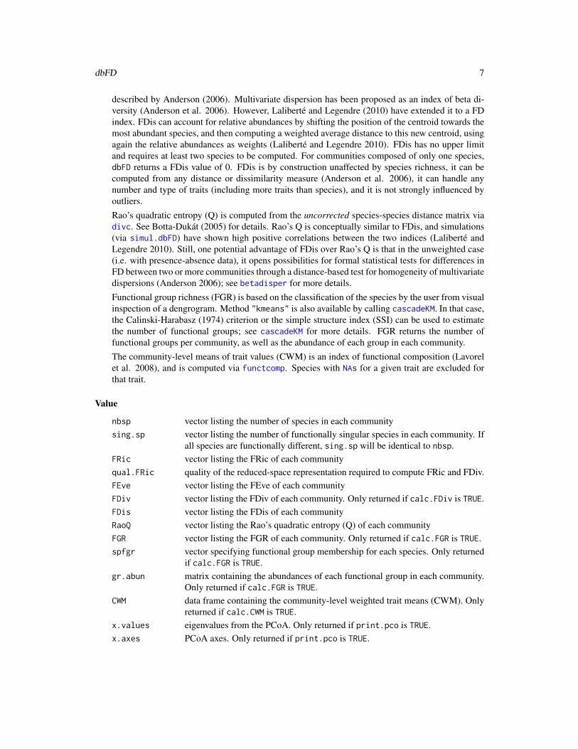
dbFD 7

described by Anderson (2006). Multivariate dispersion has been proposed as an index of beta di-versity (Anderson et al. 2006). However, Laliberté and Legendre (2010) have extended it to a FDindex. FDis can account for relative abundances by shifting the position of the centroid towards themost abundant species, and then computing a weighted average distance to this new centroid, usingagain the relative abundances as weights (Laliberté and Legendre 2010). FDis has no upper limitand requires at least two species to be computed. For communities composed of only one species,dbFD returns a FDis value of 0. FDis is by construction unaffected by species richness, it can becomputed from any distance or dissimilarity measure (Anderson et al. 2006), it can handle anynumber and type of traits (including more traits than species), and it is not strongly influenced byoutliers.Rao’s quadratic entropy (Q) is computed from the uncorrected species-species distance matrix viadivc. See Botta-Dukát (2005) for details. Rao’s Q is conceptually similar to FDis, and simulations(via simul.dbFD) have shown high positive correlations between the two indices (Laliberté andLegendre 2010). Still, one potential advantage of FDis over Rao’s Q is that in the unweighted case(i.e. with presence-absence data), it opens possibilities for formal statistical tests for differences inFD between two or more communities through a distance-based test for homogeneity of multivariatedispersions (Anderson 2006); see betadisper for more details.Functional group richness (FGR) is based on the classification of the species by the user from visualinspection of a dengrogram. Method "kmeans" is also available by calling cascadeKM. In that case,the Calinski-Harabasz (1974) criterion or the simple structure index (SSI) can be used to estimatethe number of functional groups; see cascadeKM for more details. FGR returns the number offunctional groups per community, as well as the abundance of each group in each community.The community-level means of trait values (CWM) is an index of functional composition (Lavorelet al. 2008), and is computed via functcomp. Species with NAs for a given trait are excluded forthat trait.

Value

nbsp vector listing the number of species in each communitysing.sp vector listing the number of functionally singular species in each community. If

all species are functionally different, sing.sp will be identical to nbsp.FRic vector listing the FRic of each communityqual.FRic quality of the reduced-space representation required to compute FRic and FDiv.FEve vector listing the FEve of each communityFDiv vector listing the FDiv of each community. Only returned if calc.FDiv is TRUE.FDis vector listing the FDis of each communityRaoQ vector listing the Rao’s quadratic entropy (Q) of each communityFGR vector listing the FGR of each community. Only returned if calc.FGR is TRUE.spfgr vector specifying functional group membership for each species. Only returned

if calc.FGR is TRUE.gr.abun matrix containing the abundances of each functional group in each community.

Only returned if calc.FGR is TRUE.CWM data frame containing the community-level weighted trait means (CWM). Only

returned if calc.CWM is TRUE.x.values eigenvalues from the PCoA. Only returned if print.pco is TRUE.x.axes PCoA axes. Only returned if print.pco is TRUE.

8 dbFD

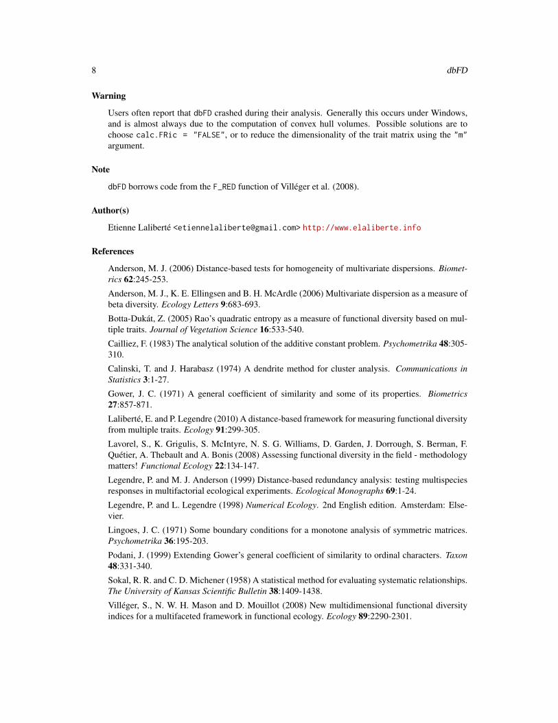
Warning

Users often report that dbFD crashed during their analysis. Generally this occurs under Windows,and is almost always due to the computation of convex hull volumes. Possible solutions are tochoose calc.FRic = "FALSE", or to reduce the dimensionality of the trait matrix using the "m"argument.

Note

dbFD borrows code from the F_RED function of Villéger et al. (2008).

Author(s)

Etienne Laliberté <[email protected]> http://www.elaliberte.info

References

Anderson, M. J. (2006) Distance-based tests for homogeneity of multivariate dispersions. Biomet-rics 62:245-253.

Anderson, M. J., K. E. Ellingsen and B. H. McArdle (2006) Multivariate dispersion as a measure ofbeta diversity. Ecology Letters 9:683-693.


Cailliez, F. (1983) The analytical solution of the additive constant problem. Psychometrika 48:305-310.

Calinski, T. and J. Harabasz (1974) A dendrite method for cluster analysis. Communications inStatistics 3:1-27.

Gower, J. C. (1971) A general coefficient of similarity and some of its properties. Biometrics27:857-871.

Laliberté, E. and P. Legendre (2010) A distance-based framework for measuring functional diversityfrom multiple traits. Ecology 91:299-305.

Lavorel, S., K. Grigulis, S. McIntyre, N. S. G. Williams, D. Garden, J. Dorrough, S. Berman, F.Quétier, A. Thebault and A. Bonis (2008) Assessing functional diversity in the field - methodologymatters! Functional Ecology 22:134-147.

Legendre, P. and M. J. Anderson (1999) Distance-based redundancy analysis: testing multispeciesresponses in multifactorial ecological experiments. Ecological Monographs 69:1-24.

Legendre, P. and L. Legendre (1998) Numerical Ecology. 2nd English edition. Amsterdam: Else-vier.

Lingoes, J. C. (1971) Some boundary conditions for a monotone analysis of symmetric matrices.Psychometrika 36:195-203.


Sokal, R. R. and C. D. Michener (1958) A statistical method for evaluating systematic relationships.The University of Kansas Scientific Bulletin 38:1409-1438.

Villéger, S., N. W. H. Mason and D. Mouillot (2008) New multidimensional functional diversityindices for a multifaceted framework in functional ecology. Ecology 89:2290-2301.


dbFD 9

See Also

gowdis, functcomp, fdisp, simul.dbFD, divc, treedive, betadisper

Examples

# mixed trait types, NA'sex1 <- dbFD(dummy$trait, dummy$abun)ex1

# add variable weights# 'cailliez' correction is used because 'sqrt' does not workw<-c(1, 5, 3, 2, 5, 2, 6, 1)ex2 <- dbFD(dummy$trait, dummy$abun, w, corr="cailliez")

# if 'x' is a distance matrixtrait.d <- gowdis(dummy$trait)ex3 <- dbFD(trait.d, dummy$abun)ex3

# one numeric trait, one NAnum1 <- dummy$trait[,1] ; names(num1) <- rownames(dummy$trait)ex4 <- dbFD(num1, dummy$abun)ex4

# one ordered trait, one NAord1 <- dummy$trait[,5] ; names(ord1) <- rownames(dummy$trait)ex5 <- dbFD(ord1, dummy$abun)ex5

# one nominal trait, one NAfac1 <- dummy$trait[,3] ; names(fac1) <- rownames(dummy$trait)ex6 <- dbFD(fac1, dummy$abun)ex6

# example with real data from New Zealand short-tussock grasslands# 'lingoes' correction used because 'sqrt' does not work in that caseex7 <- dbFD(tussock$trait, tussock$abun, corr = "lingoes")

## Not run:# calc.FGR = T, 'ward'ex7 <- dbFD(dummy$trait, dummy$abun, calc.FGR = T)ex7

# calc.FGR = T, 'kmeans'ex8 <- dbFD(dummy$trait, dummy$abun, calc.FGR = T,clust.type = "kmeans")ex8

# ward clustering to compute FGRex9 <- dbFD(tussock$trait, tussock$abun,corr = "cailliez", calc.FGR = TRUE, clust.type = "ward")

10 fdisp

# choose 'g' for number of groups# 6 groups seems to make good ecological senseex9

# however, calinksi criterion in 'kmeans' suggests# that 6 groups may not be optimalex10 <- dbFD(tussock$trait, tussock$abun, corr = "cailliez",calc.FGR = TRUE, clust.type = "kmeans", km.sup.gr = 10)

## End(Not run)

dummy Dummy Functional Trait Dataset

Description

A dummy dataset containing 8 species and 8 functional traits (2 continuous, 2 nominal, 2 ordinal,and 2 binary), with some missing values. Also includes a matrix of species abundances from 10communities.

Usage

dummy

Format

trait data frame of 8 functional traits on 8 species

abun matrix of abundances of the 8 species from 10 communities

Source

Etienne Laliberté <[email protected]>

fdisp Functional Dispersion

Description

fdisp measures the functional dispersion (FDis) of a set of communities, as described by Lalibertéand Legendre (2010).

Usage

fdisp(d, a, tol = 1e-07)

fdisp 11

Arguments

d a species-by- species distance matrix computed from functional traits, such asthat returned by dist or gowdis. NAs are not allowed.

a matrix containing the abundances of the species in d (or presence-absence, i.e.0 or 1). Rows are sites and species are columns. Can be missing, in which casefdisp assumes that there is only one community with equal abundances of allspecies. NAs will be replaced by 0. The number of species (columns) in a mustmatch the number of species in d. In addition, the species labels in a and d mustbe identical and in the same order.

tol tolerance threshold to test whether the distance matrix is Euclidean : an eigen-value is considered positive if it is larger than -tol*λ1, where λ1 is the largesteigenvalue.

Details

fdisp computes, for a set of communities, the average distance of individual objects (species) inPCoA space from any distance or dissimilarity measure, as described by Anderson (2006). Theaverage distance to the centroid is a measure of multivariate dispersion and as been suggested as anindex of beta diversity (Anderson et al. 2006). However, in fdisp both the centroid and the averagedistance to this centroid can be weighted by individual objects. In other words, fdisp returnsthe weighted average distance to the weighted centroid. This was suggested so that multivariatedispersion could be used as a multidimensional functional diversity (FD) index that can be weightedby species abundances. This FD index has been called functional dispersion (FDis) and is describedby Laliberté and Legendre (2010).

In sum, FDis can account for relative abundances by shifting the position of the centroid towardsthe most abundant species, and then computing a weighted average distance to this new centroid,using again the relative abundances as weights (Laliberté and Legendre 2010). FDis has no upperlimit and requires at least two species to be computed. For communities composed of only onespecies, dbFD returns a FDis value of 0. FDis is by construction unaffected by species richness, itcan be computed from any distance or dissimilarity measure (Anderson et al. 2006), it can handleany number and type of traits (including more traits than species), and it is not strongly influencedby outliers.

FDis is conceptually similar to Rao’s quadratic entropy Q (Botta-Dukát 2005), and simulations(via simul.dbFD) have shown high positive correlations between the two indices (Laliberté andLegendre 2010). Still, one potential advantage of FDis over Rao’s Q is that in the unweighted case(i.e. with presence-absence data), it opens possibilities for formal statistical tests for differences inFD between two or more communities through a distance-based test for homogeneity of multivariatedispersions (Anderson 2006); see betadisper for more details.

Corrections for PCoA axes corresponding to negative eigenvalues are applied following Anderson(2006); see also betadisper for more details on these corrections.

Value

FDis vector listing the FDis of each community

eig vector listing the eigenvalues of the PCoA

vectors matrix containing the PCoA axes

12 functcomp

Note

fdisp is implemented in dbFD and is used to compute the functional dispersion (FDis) index.

Author(s)


References

Anderson, M. J. (2006) Distance-based tests for homogeneity of multivariate dispersions. Biomet-rics 62:245-253.

Anderson, M. J., K. E. Ellingsen and B. H. McArdle (2006) Multivariate dispersion as a measure ofbeta diversity. Ecology Letters 9:683-693.


Laliberté, E. and P. Legendre (2010) A distance-based framework for measuring functional diversityfrom multiple traits. Ecology 91299:305.

See Also

dbFD for computing multidimensional FD indices and betadisper from which fdisp borrowssome code.

Examples

# dummy datasetdummy.dist <- gowdis(dummy$trait)ex1 <- fdisp(dummy.dist, dummy$abun)ex1

# example with real data from New Zealand short-tussock grasslandsex2 <- fdisp(gowdis(tussock$trait), tussock$abun)ex2

functcomp Functional Composition

Description

functcomp returns the functional composition of a set of communities, as measured by the community-level weighted means of trait values (CWM; e.g. Lavorel et al. 2008).

Usage

functcomp(x, a, CWM.type = c("dom", "all"), bin.num = NULL)


functcomp 13

Arguments

x matrix or data frame containing the functional traits. Traits can be numeric,ordered, or factor. Binary traits should be numeric and only contain 0 and 1.character traits will be converted to factor. For a given trait, species with NAare excluded.

a matrix containing the abundances of the species in x (or presence-absence, i.e. 0or 1). Rows are sites and species are columns. The number of species (columns)in a must match the number of species (rows) in x. In addition, the species labelsin a and x must be identical and in the same order. NAs will be replaced by 0.

CWM.type character string indicating how nominal, binary and ordinal traits should be han-dled. See ‘details’.

bin.num vector indicating binary traits to be treated as continuous.

Details

functcomp computes the community-level weighted means of trait values for a set of communi-ties (i.e. sites). For a continuous trait, CWM is the mean trait value of all species present in thecommunity (after excluding species with NAs), weighted by their relative abundances.

For ordinal, nominal and binary traits, either the dominant class is returned (when CWM.type is"dom"), or the abundance of each individual class is returned (when CWM.type is "all").

The default behaviour of binary traits being treated as nominal traits can be over-ridden by specify-ing bin.num, in which case they are treated as numeric traits.

When CWM.type = "dom", if the maximum abundance value is shared between two or more classes,then one of these classes is randomly selected for CWM. Because species with NAs for a giventrait are excluded for that trait, it is possible that when CWM.type is set to "all", the sum of theabundances of all classes for a given ordinal/nominal/binary trait does not equal the sum of thespecies abundances. Thus, it is definitely not recommended to have NAs for very abundant species,as this will lead to biased estimates of functional composition.

Value

a data frame containing the CWM values of each trait for each community.

Note

functcomp is implemented in dbFD and will be returned if calc.CWM is TRUE.

Author(s)


References

Lavorel, S., K. Grigulis, S. McIntyre, N. S. G. Williams, D. Garden, J. Dorrough, S. Berman, F.Quétier, A. Thébault and A. Bonis (2008) Assessing functional diversity in the field - methodologymatters! Functional Ecology 22:134-147.


14 gowdis

See Also

dbFD for measuring distance-based multidimensional functional diversity indices, including CWM.

Examples

# for ordinal, nominal and binary variables# returns only the most frequent classex1 <- functcomp(dummy$trait, dummy$abun)ex1

# returns the frequencies of each classex2 <- functcomp(dummy$trait, dummy$abun, CWM.type = "all")ex2

# example with real data from New Zealand short-tussock grasslandsex3 <- functcomp(tussock$trait, tussock$abun)ex3

gowdis Gower Dissimilarity

Description

gowdis measures the Gower (1971) dissimilarity for mixed variables, including asymmetric binaryvariables. Variable weights can be specified. gowdis implements Podani’s (1999) extension toordinal variables.

Usage

gowdis(x, w, asym.bin = NULL, ord = c("podani", "metric", "classic"))

Arguments

x matrix or data frame containing the variables. Variables can be numeric, ordered,or factor. Symmetric or asymmetric binary variables should be numeric andonly contain 0 and 1. character variables will be converted to factor. NAs aretolerated.

w vector listing the weights for the variables in x. Can be missing, in which caseall variables have equal weights.

asym.bin vector listing the asymmetric binary variables in x.

ord character string specifying the method to be used for ordinal variables (i.e.ordered). "podani" refers to Eqs. 2a-b of Podani (1999), while "metric"refers to his Eq. 3 (see ‘details’); both options convert ordinal variables to ranks."classic" simply treats ordinal variables as continuous variables. Can be ab-breviated.

gowdis 15

Details

gowdis computes the Gower (1971) similarity coefficient exactly as described by Podani (1999),then converts it to a dissimilarity coefficient by using D = 1− S. It integrates variable weights asdescribed by Legendre and Legendre (1998).

Let X = {xij} be a matrix containing n objects (rows) and m columns (variables). The similarityGjk between objects j and k is computed as

Gjk =

∑ni=1 wijksijk∑n

i=1 wijk

,

where wijk is the weight of variable i for the j-k pair, and sijk is the partial similarity of variable ifor the j-k pair,

and where wijk = 0 if objects j and k cannot be compared because xij or xik is unknown (i.e. NA).

For binary variables, sijk = 0 if xij 6= xik, and sijk = 1 if xij = xik = 1 or if xij = xik = 0.

For asymmetric binary variables, same as above except that wijk = 0 if xij = xik = 0.

For nominal variables, sijk = 0 if xij 6= xik and sijk = 1 if xij = xik.

For continuous variables,

sijk = 1− |xij − xik|xi.max − xi.min

where xi.max and xi.min are the maximum and minimum values of variable i, respectively.

For ordinal variables, when ord = "podani" or ord = "metric", all xij are replaced by theirranks rij determined over all objects (such that ties are also considered), and then

if ord = "podani"

sijk = 1 if rij = rik, otherwise

sijk = 1− |rij − rik| − (Tij − 1)/2− (Tik − 1)/2

ri.max − ri.min − (Ti.max − 1)/2− (Ti.min − 1)/2

where Tij is the number of objects which have the same rank score for variable i as object j (in-cluding j itself), Tik is the number of objects which have the same rank score for variable i asobject k (including k itself), ri.max and ri.min are the maximum and minimum ranks for variable i,respectively, Ti,max is the number of objects with the maximum rank, and Ti.min is the number ofobjects with the minimum rank.

if ord = "metric"

sijk = 1− |rij − rik|ri.max − ri.min

When ord = "classic", ordinal variables are simply treated as continuous variables.

16 gowdis

Value

an object of class dist with the following attributes: Labels, Types (the variable types, where ’C’is continuous/numeric, ’O’ is ordinal, ’B’ is symmetric binary, ’A’ is asymmetric binary, and ’N’ isnominal), Size, Metric.

Author(s)

Etienne Laliberté <[email protected]> http://www.elaliberte.info, with somehelp from Philippe Casgrain for the C interface.

References

Gower, J. C. (1971) A general coefficient of similarity and some of its properties. Biometrics27:857-871.



See Also

daisy is similar but less flexible, since it does not include variable weights and does not treat ordinalvariables as described by Podani (1999). Using ord = "classic" reproduces the behaviour ofdaisy.

Examples

ex1 <- gowdis(dummy$trait)ex1

# check attributesattributes(ex1)

# to include weightsw <- c(4,3,5,1,2,8,3,6)ex2 <- gowdis(dummy$trait, w)ex2

# variable 7 as asymmetric binaryex3 <- gowdis(dummy$trait, asym.bin = 7)ex3

# example with trait data from New Zealand vascular plant speciesex4 <- gowdis(tussock$trait)


mahaldis 17

mahaldis Mahalanobis Distance

Description

mahaldis measures the pairwise Mahalanobis (1936) distances between individual objects.

Usage

mahaldis(x)

Arguments

x matrix containing the variables. NAs are not tolerated.

Details

mahaldis computes the Mahalanobis (1936) distances between individual objects. The Maha-lanobis distance takes into account correlations among variables and does not depend on the scalesof the variables.

mahaldis builds on the fact that type-II principal component analysis (PCA) preserves the Maha-lanobis distance among objects (Legendre and Legendre 2012). Therefore, mahaldis first performsa type-II PCA on standardized variables, and then computes the Euclidean distances among (repo-sitioned) objects whose positions are given in the matrix G. This is equivalent to the Mahalanobisdistances in the space of the original variables (Legendre and Legendre 2012).

Value

an object of class dist.

Author(s)

Pierre Legendre <[email protected]>

http://www.bio.umontreal.ca/legendre/indexEn.html

Ported to FD by Etienne Laliberté.

References


See Also

mahalanobis computes the Mahalanobis distances among groups of objects, not individual objects.

http://www.bio.umontreal.ca/legendre/indexEn.html

18 maxent

Examples

mat <- matrix(rnorm(100), 50, 20)

ex1 <- mahaldis(mat)

# check attributesattributes(ex1)

maxent Estimating Probabilities via Maximum Entropy: Improved IterativeScaling

Description

maxent returns the probabilities that maximize the entropy conditional on a series of constraints thatare linear in the features. It relies on the Improved Iterative Scaling algorithm of Della Pietra et al.(1997). It has been used to predict the relative abundances of a set of species given the trait valuesof each species and the community-aggregated trait values at a site (Shipley et al. 2006; Shipley2009; Sonnier et al. 2009).

Usage

maxent(constr, states, prior, tol = 1e-07, lambda = FALSE)

Arguments

constr vector of macroscopical constraints (e.g. community-aggregated trait values).Can also be a matrix or data frame, with constraints as columns and data sets(e.g. sites) as rows.

states vector, matrix or data frame of states (columns) and their attributes (rows).

prior vector, matrix or data frame of prior probabilities of states (columns). Can bemissing, in which case a maximally uninformative prior is assumed (i.e. uniformdistribution).

tol tolerance threshold to determine convergence. See ‘details’ section.

lambda Logical. Should λ-values be returned?

Details

The biological model of community assembly through trait-based habitat filtering (Keddy 1992) hasbeen translated mathematically via a maximum entropy (maxent) model by Shipley et al. (2006)and Shipley (2009). A maxent model contains three components: (i) a set of possible states and theirattributes, (ii) a set of macroscopic empirical constraints, and (iii) a prior probability distributionq = [qj ].

In the context of community assembly, states are species, macroscopic empirical constraints arecommunity-aggregated traits, and prior probabilities q are the relative abundances of species ofthe regional pool (Shipley et al. 2006, Shipley 2009). By default, these prior probabilities q are

maxent 19

maximally uninformative (i.e. a uniform distribution), but can be specificied otherwise (Shipley2009, Sonnier et al. 2009).

To facilitate the link between the biological model and the mathematical model, in the followingdescription of the algorithm states are species and constraints are traits.

Note that if constr is a matrix or data frame containing several sets (rows), a maxent model is runon each individual set. In this case if prior is a vector, the same prior is used for each set. Adifferent prior can also be specified for each set. In this case, the number of rows in prior must beequal to the number of rows in constr.

If q is not specified, set pj = 1/S for each of the S species (i.e. a uniform distribution), where pjis the probability of species j, otherwise pj = qj .

Calulate a vector c = [ci ] = {c1, c2, . . . , cT }, where ci =

S∑j=1

tij ; i.e. each ci is the sum of the

values of trait i over all species, and T is the number of traits.

Repeat for each iteration k until convergence:

1. For each trait ti (i.e. row of the constraint matrix) calculate:

γi(k) = ln

t̄i

S∑j=1

(pj(k) tij)

(

1

ci

)

This is simply the natural log of the known community-aggregated trait value to the calculatedcommunity-aggregated trait value at this step in the iteration, given the current values of the proba-bilities. The whole thing is divided by the sum of the known values of the trait over all species.

2. Calculate the normalization term Z:

Z(k) =

S∑

j=1

pj(k) e

(T∑

i=1

γi(k) tij

)3. Calculate the new probabilities pj of each species at iteration k + 1:

pj(k + 1) =pj(k) e

(T∑

i=1

γi(k) tij

)Z(k)

4. If |max (p (k + 1)− p (k)) | ≤ tolerance threshold (i.e. argument tol) then stop, else repeatsteps 1 to 3.

When convergence is achieved then the resulting probabilities (p̂j) are those that are as close aspossible to qj while simultaneously maximize the entropy conditional on the community-aggregatedtraits. The solution to this problem is the Gibbs distribution:

20 maxent

p̂j =qje

(−

T∑i=1

λitij

)

S∑j=1

qje

(−

T∑i=1

λitij

) =qje

(−

T∑i=1

λitij

)Z

This means that one can solve for the Langrange multipliers (i.e. weights on the traits, λi) bysolving the linear system of equations:

ln (p̂1)ln (p̂2)

...ln (p̂S)

= (λ1, λ2, . . . , λT )

t11 t12 . . . t1S − ln(Z)

t21 t22... t2S − ln(Z)

......

......

tT1 tT2 . . . tTS − ln(Z)

− ln(Z)

This system of linear equations has T+1 unknowns (the T values of λ plus ln(Z)) and S equations.So long as the number of traits is less than S − 1, this system is soluble. In fact, the solution is thewell-known least squares regression: simply regress the values ln(p̂j) of each species on the traitvalues of each species in a multiple regression.

The intercept is the value of ln(Z) and the slopes are the values of λi and these slopes (Lagrangemultipliers) measure by how much the ln(p̂j), i.e. the ln(relative abundances), changes as the valueof the trait changes.

maxent.test provides permutation tests for maxent models (Shipley 2010).

Value

prob vector of predicted probabilities

moments vector of final moments

entropy Shannon entropy of prob

iter number of iterations required to reach convergence

lambda λ-values, only returned if lambda = T

constr macroscopical constraints

states states and their attributes

prior prior probabilities

Author(s)

Bill Shipley <[email protected]>

http://pages.usherbrooke.ca/jshipley/recherche/

Ported to FD by Etienne Laliberté.

http://pages.usherbrooke.ca/jshipley/recherche/

maxent 21

References

Della Pietra, S., V. Della Pietra, and J. Lafferty (1997) Inducing features of random fields. IEEETransactions Pattern Analysis and Machine Intelligence 19:1-13.

Keddy, P. A. (1992) Assembly and response rules: two goals for predictive community ecology.Journal of Vegetation Science 3:157-164.

Shipley, B., D. Vile, and É. Garnier (2006) From plant traits to plant communities: a statisticalmechanistic approach to biodiversity. Science 314: 812–814.

Shipley, B. (2009) From Plant Traits to Vegetation Structure: Chance and Selection in the Assemblyof Ecological Communities. Cambridge University Press, Cambridge, UK. 290 pages.

Shipley, B. (2010) Inferential permutation tests for maximum entropy models in ecology. Ecologyin press.

Sonnier, G., Shipley, B., and M. L. Navas. 2009. Plant traits, species pools and the predictionof relative abundance in plant communities: a maximum entropy approach. Journal of VegetationScience in press.

See Also

functcomp to compute community-aggregated traits, and maxent.test for the permutation testsproposed by Shipley (2010).

Another faster version of maxent for multicore processors called maxentMC is available from Eti-enne Laliberté (<[email protected]>). It’s exactly the same as maxent but makesuse of the multicore, doMC, and foreach packages. Because of this, maxentMC only works onPOSIX-compliant OS’s (essentially anything but Windows).

Examples

# an unbiased 6-sided dice, with mean = 3.5# what is the probability associated with each side,# given this constraint?maxent(3.5, 1:6)

# a biased 6-sided dice, with mean = 4maxent(4, 1:6)

# example with tussock datasettraits <- tussock$trait[, c(2:7, 11)] # use only continuous traitstraits <- na.omit(traits) # remove 2 species with NA'sabun <- tussock$abun[, rownames(traits)] # abundance matrixabun <- t(apply(abun, 1, function(x) x / sum(x) )) # relative abundancesagg <- functcomp(traits, abun) # community-aggregated traitstraits <- t(traits) # transpose matrix

# run maxent on site 1 (first row of abun), all speciespred.abun <- maxent(agg[1,], traits)

## Not run:# do the constraints give predictive ability?maxent.test(pred.abun, obs = abun[1,], nperm = 49)

22 maxent.test

## End(Not run)

maxent.test Inferential Permutation Tests for Maximum Entropy Models

Description

maxent.test performs the permutation tests proposed by Shipley (2010) for maximum entropymodels. Two different null hypotheses can be tested: 1) the information encoded in the entire set ofconstraints C is irrelevant for predicting the probabilities, and 2) the information encoded in subsetB of the entire set of constraints C = A ∪ B is irrelevant for predicting the probabilities. A plotcan be returned to facilitate interpretation.

Usage

maxent.test(model, obs, sub.c, nperm = 99, quick = TRUE,alpha = 0.05, plot = TRUE)

Arguments

model list returned by maxent.

obs vector, matrix or data frame of observed probabilities of the states (columns).

sub.c character or numeric vector specifying the subset of constraints B associatedwith null hypothesis 2. If missing, null hypothesis 1 is tested.

nperm number of permutations for the test.

quick if TRUE, the algorithm stops when alpha is outside the confidence interval of theP-value. Can be useful to speed up the routine.

alpha desired alpha-level for the test. Only relevant if quick is TRUE.

plot if TRUE, a plot is returned to facilitate interpretation.

Details

maxent.test is a direct translation of the permutation tests described by Shipley (2010). Pleaserefer to this article for details.

Using quick = FALSE will return the true null probability for a given nperm. However, if nperm islarge (a rule-of-thumb is >= 999 permutations for allowing inference at α = 0.05), this can take avery long time. Using quick = TRUE is a much faster and highly recommended alternative if one isonly interested in accepting/rejecting the null hypothesis at the specified α-level given by argumentalpha.

If maxent was run with multiple data sets (i.e. if constr had more than one row), then maxent.testperforms the test for all sets simultaneously, following the ‘omnibus’ procedure described by Ship-ley (2010).

The following measure of fit between observed and predicted probabilities is returned:

maxent.test 23

fit = 1−

D∑j=1

S∑i=1

(oij − pij)2

D∑j=1

S∑i=1

(oij − qij)2

where oij , pij , and qij are the observed, predicted and prior probabilities of state i from data set j,respectively, S is the number of states, and D the number of data sets (i.e. rows in obs). A value of1 indicates perfect predictive capacity, while a value near zero indicates that the constraints provideno additional information beyond what is already contained in the prior q (Sonnier et al. 2009).

Value

fit measure of fit giving the predictive ability of the entire set of constraints C,beyond that already provided by the prior distribution.

fit.a measure of fit giving the predictive ability of the subset of constraints A, beyondthat already provided by the prior distribution; only returned if sub.c is specified

r2 Pearson r2 between observed and predicted probabilities, using the entire set ofconstraints C

r2.a Pearson r2 between observed and predicted probabilities, using the subset ofconstraints A; only returned if sub.c is specified

r2.q Pearson r2 between observed and prior probabilities; only returned when sub.cis missing

obs.stat observed statistic used for the permutation test; see Shipley (2010)

nperm number of permutations; can be smaller than the specified nperm when quick isTRUE

pval P-value

ci.pval approximate confidence intervals of the P-value

Warning

maxent.test is a computationally intensive function. The tests can take a very long time whennperm is large and quick = FALSE. It is highly recommended to use quick = TRUE because ofthis, unless you are interested in obtaining the true null probability.

Author(s)




24 simul.dbFD

References

Sonnier, G., Shipley, B., and M. L. Navas. 2009. Plant traits, species pools and the predictionof relative abundance in plant communities: a maximum entropy approach. Journal of VegetationScience in press.

Shipley, B. (2010) Inferential permutation tests for maximum entropy models in ecology. Ecologyin press.

See Also

maxent to run the maximum entropy model that is required by maxent.test.

Another faster version of maxent.test for multicore processors called maxent.testMC is availablefrom Etienne Laliberté (<[email protected]>). It’s exactly the same as maxent.testbut makes use of the multicore, doMC, and foreach packages. Because of this, maxentMC onlyworks on POSIX-compliant OS’s (essentially anything but Windows).

Examples

# example with tussock datasettraits <- tussock$trait[, c(2:7, 11)] # use only continuous traitstraits <- na.omit(traits) # remove 2 species with NA'sabun <- tussock$abun[, rownames(traits)] # abundance matrixabun <- t(apply(abun, 1, function(x) x / sum(x) )) # relative abundancesagg <- functcomp(traits, abun) # community-aggregated traitstraits <- t(traits) # transpose matrix

# run maxent on site 1 (first row of abun), all speciespred.abun <- maxent(agg[1,], traits)

## Not run:# do the constraints give predictive ability?maxent.test(pred.abun, obs = abun[1,], nperm = 49)

# are height, LDMC, and leaf [N] important constraints?maxent.test(pred.abun, obs = abun[1,], sub.c = c("height","LDMC", "leafN"), nperm = 49)

## End(Not run)

simul.dbFD Simulations to Explore Relationships Between Functional DiversityIndices

Description

simul.dbFD generates artificial communities of species with artificial functional traits. Differentfunctional diversity (FD) indices are computed from these communities using dbFD to explore theirinter-relationships.

simul.dbFD 25

Usage

simul.dbFD(s = c(5, 10, 15, 20, 25, 30, 35, 40), t = 3,r = 10, p = 100, tr.method = c("unif", "norm", "lnorm"),abun.method = c("lnorm", "norm", "unif"), w.abun = TRUE)

Arguments

s vector listing the different levels of species richness used in the simulations

t number of traits

r number of replicates per species richness level

p number of species in the common species pool

tr.method character string indicating the sampling distribution for the traits. "unif" is auniform distribution, "norm" is a normal distribution, and "lnorm" is a lognor-mal distribution.

abun.method character string indicating the sampling distribution for the species abundances.Same as for tr.method.

w.abun logical; should FDis, FEve, FDiv, and Rao’s quadratic entropy (Q) be weightedby species abundances?

Value

A list contaning the following elements:

results data frame containing the results of the simulations

traits matrix containing the traits

abun matrix containing the abundances

abun.gamma species abundances from the pooled set of communities

FDis.gamma FDis of the pooled set of communities

FDis.mean mean FDis from all communities

FDis.gamma and FDis.mean can be used to explore the set concavity criterion (Ricotta 2005) forFDis.

A graph plotting the results of the simulations is also returned.

Warning

The simulations performed by simul.dbFD can take several hours if length(s) and/or r is large.Run a test with the default parameters first.

Author(s)



26 tussock

References

Laliberté, E. and P. Legendre (2010) A distance-based framework for measuring functional diversityfrom multiple traits. Ecology 91299:305.

Ricotta, C. (2005) A note on functional diversity measures. Basic and Applied Ecology 6:479-486.

See Also

dbFD, the function called in simul.dbFD

Examples

# this should take just a few minutes## Not run:ex1 <- simul.dbFD(s = c(10, 20, 30, 40, 50), r = 5)ex1

## End(Not run)

tussock Functional Composition of Short-Tussock Grasslands

Description

tussock contains data on 16 functional traits measured on 53 vascular plant species from NewZealand short-tussock grasslands. It also contains the relative abundances (percent cover) of these53 species from 30 8x50-m plots.

Usage

tussock

Format

tussock is a list of 2 components:

trait data frame of 16 functional traits measured on 53 plant species: growth form (sensu Cornelis-sen et al. 2003), reproductive plant height (m), leaf dry matter content (mg g−1), leaf nitrogenconcentration (mg g−1), leaf phosphorous concentration (mg g−1), leaf sulphur concentra-tion (mg g−1), specific leaf area (m2 kg−1), nutrient uptake strategy (sensu Cornelissen etal. 2003), Raunkiaer life form, clonality, leaf size (mm2), primary dispersal mode, seed mass(mg), resprouting capacity, pollination syndrome, and lifespan (an ordinal variable stored asordered).

abun matrix containing the relative abundances (percent cover) of the 53 species in 30 plots

tussock 27

Details

The functional traits were measured using standardized methodologies (Cornelissen et al. 2003).Each of the 30 experimental plots from which species cover was estimated is 8x50 m. Relativeabundances of all vascular plant species were estimated in November 2007. To do so, 20 1x1-m quadrats per plot were randomly positioned along two longitudinal transects and cover of eachspecies was estimated using a modified Braun-Blanquet scale. This data was pooled at the plot scaleto yield the percent cover data.

Source



References

Cornelissen, J. H. C., S. Lavorel, E. Garnier, S. Diaz, N. Buchmann, D. E. Gurvich, P. B. Reich,H. ter Steege, H. D. Morgan, M. G. A. van der Heijden, J. G. Pausas and H. Poorter. (2003) Ahandbook of protocols for standardised and easy measurement of plant functional traits worldwide.Australian Journal of Botany 51:335-380.

Laliberté, E., Norton, D. A. and D. Scott. (2008) Impacts of rangeland development on plantfunctional diversity, ecosystem processes and services, and resilience. Global Land Project (GLP)Newsletter 4:4-6.

Scott, D. (1999) Sustainability of New Zealand high-country pastures under contrasting develop-ment inputs. 1. Site, and shoot nutrients. New Zealand Journal of Agricultural Research 42:365-383.


Index

∗Topic datagensimul.dbFD, 24

∗Topic datasetsdummy, 10tussock, 26

∗Topic distributionmaxent, 18maxent.test, 22

∗Topic mathmaxent, 18maxent.test, 22

∗Topic modelsmaxent, 18maxent.test, 22

∗Topic multivariatedbFD, 3fdisp, 10functcomp, 12gowdis, 14mahaldis, 17

∗Topic packageFD-package, 2

betadisper, 7, 9, 11, 12

cailliez, 6cascadeKM, 5, 7character, 4, 13, 14

daisy, 16dbFD, 2, 3, 12–14, 24, 26dist, 4, 6, 11, 16, 17dist.binary, 5, 6divc, 5, 7, 9dudi.pco, 6dummy, 10

factor, 4–6, 13, 14FD (FD-package), 2FD-package, 2

fdisp, 6, 9, 10functcomp, 5, 7, 9, 12, 21

gowdis, 2, 4–6, 9, 11, 14

hclust, 5

is.euclid, 6

lingoes, 6

mahalanobis, 17mahaldis, 17maxent, 2, 18, 22, 24maxent.test, 20, 21, 22

NA, 2, 4, 6, 7, 11, 13–15, 17numeric, 4, 6, 13, 14

ordered, 4, 6, 13, 14, 26

quasieuclid, 6

simul.dbFD, 7, 9, 11, 24

treedive, 9tussock, 26

28

Documents

Package ‘FD’ ‘FD’ February 19, 2015 Type Package Title Measuring functional diversity (FD) from multiple traits, and other tools for functional ecology