Package ‘elsa’

Package ‘elsa’March 19, 2020

Type Package

Title Entropy-Based Local Indicator of Spatial Association

Version 1.1-28

Date 2020-03-13

Depends methods, sp (>= 1.2-0), raster, R (>= 3.0.0)

Suggests knitr, rmarkdown

DescriptionA framework that provides the methods for quantifying entropy-based local indicator of spatial as-sociation (ELSA) that can be used for both continuous and categorical data. In addition, this pack-age offers other methods to measure local indicators of spatial associations (LISA). Further-more, global spatial structure can be measured using a variogram-like diagram, called entro-gram. For more information, please check that paper: Naimi, B., Hamm, N. A., Groen, T. A., Skid-more, A. K., Toxopeus, A. G., & Alibakhshi, S. (2019) <doi:10.1016/j.spasta.2018.10.001>.

License GPL (>= 3)

VignetteBuilder knitr

URL http://r-gis.net

BugReports https://github.com/babaknaimi/elsa/issues/

NeedsCompilation yes

Author Babak Naimi [cre, aut] (<https://orcid.org/0000-0001-5431-2729>),Roger Bivand [ctb] (part of the dnn C code, from the spdep package),William Venables [ctb] (part of the dnn C code, taken from the spdeppackage),Brian Ripley [ctb] (part of the dnn C code, taken from the spdeppackage)

Maintainer Babak Naimi <[email protected]>

Repository CRAN

Date/Publication 2020-03-19 14:30:09 UTC

1

http://r-gis.net

https://github.com/babaknaimi/elsa/issues/

2 categorize

R topics documented:categorize . . . . . . . . . . . . . . . . . . . . . . . . . . . . . . . . . . . . . . . . . . 2correlogram . . . . . . . . . . . . . . . . . . . . . . . . . . . . . . . . . . . . . . . . . 3dif2list . . . . . . . . . . . . . . . . . . . . . . . . . . . . . . . . . . . . . . . . . . . . 4dneigh . . . . . . . . . . . . . . . . . . . . . . . . . . . . . . . . . . . . . . . . . . . . 6elsa . . . . . . . . . . . . . . . . . . . . . . . . . . . . . . . . . . . . . . . . . . . . . 8elsa.test . . . . . . . . . . . . . . . . . . . . . . . . . . . . . . . . . . . . . . . . . . . 10entrogram . . . . . . . . . . . . . . . . . . . . . . . . . . . . . . . . . . . . . . . . . . 11Entrogram-class . . . . . . . . . . . . . . . . . . . . . . . . . . . . . . . . . . . . . . . 13lisa . . . . . . . . . . . . . . . . . . . . . . . . . . . . . . . . . . . . . . . . . . . . . . 13moran . . . . . . . . . . . . . . . . . . . . . . . . . . . . . . . . . . . . . . . . . . . . 15nclass . . . . . . . . . . . . . . . . . . . . . . . . . . . . . . . . . . . . . . . . . . . . 16neighbours-class . . . . . . . . . . . . . . . . . . . . . . . . . . . . . . . . . . . . . . 17Variogram . . . . . . . . . . . . . . . . . . . . . . . . . . . . . . . . . . . . . . . . . . 18

Index 20

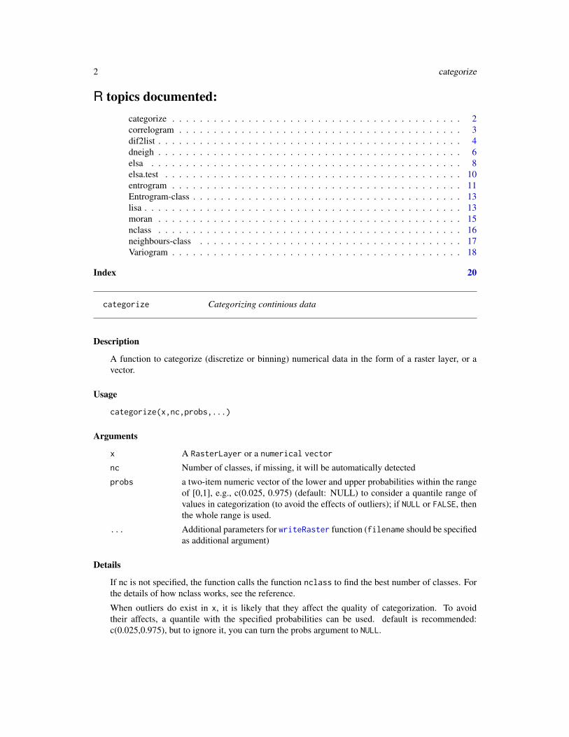
categorize Categorizing continious data

Description

A function to categorize (discretize or binning) numerical data in the form of a raster layer, or avector.

Usage

categorize(x,nc,probs,...)

Arguments

x A RasterLayer or a numerical vector

nc Number of classes, if missing, it will be automatically detected

probs a two-item numeric vector of the lower and upper probabilities within the rangeof [0,1], e.g., c(0.025, 0.975) (default: NULL) to consider a quantile range ofvalues in categorization (to avoid the effects of outliers); if NULL or FALSE, thenthe whole range is used.

... Additional parameters for writeRaster function (filename should be specifiedas additional argument)

Details

If nc is not specified, the function calls the function nclass to find the best number of classes. Forthe details of how nclass works, see the reference.

When outliers do exist in x, it is likely that they affect the quality of categorization. To avoidtheir affects, a quantile with the specified probabilities can be used. default is recommended:c(0.025,0.975), but to ignore it, you can turn the probs argument to NULL.

correlogram 3

Value

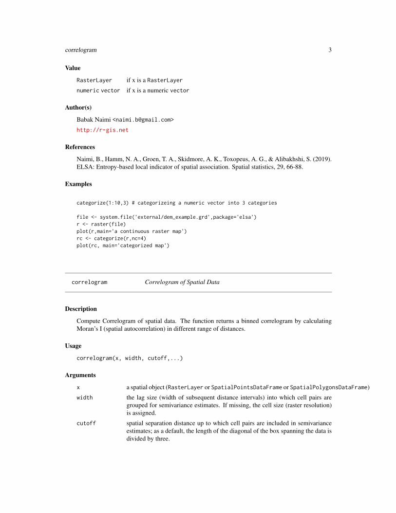
RasterLayer if x is a RasterLayer

numeric vector if x is a numeric vector

Author(s)

Babak Naimi <[email protected]>

http://r-gis.net

References

Naimi, B., Hamm, N. A., Groen, T. A., Skidmore, A. K., Toxopeus, A. G., & Alibakhshi, S. (2019).ELSA: Entropy-based local indicator of spatial association. Spatial statistics, 29, 66-88.

Examples

categorize(1:10,3) # categorizeing a numeric vector into 3 categories

file <- system.file('external/dem_example.grd',package='elsa')r <- raster(file)plot(r,main='a continuous raster map')rc <- categorize(r,nc=4)plot(rc, main='categorized map')

correlogram Correlogram of Spatial Data

Description

Compute Correlogram of spatial data. The function returns a binned correlogram by calculatingMoran’s I (spatial autocorrelation) in different range of distances.

Usage

correlogram(x, width, cutoff,...)

Arguments

x a spatial object (RasterLayer or SpatialPointsDataFrame or SpatialPolygonsDataFrame)

width the lag size (width of subsequent distance intervals) into which cell pairs aregrouped for semivariance estimates. If missing, the cell size (raster resolution)is assigned.

cutoff spatial separation distance up to which cell pairs are included in semivarianceestimates; as a default, the length of the diagonal of the box spanning the data isdivided by three.

http://r-gis.net

4 dif2list

... Additional arguments including zcol (when x is Spatial* object, specifies thename of the variable in the dataset; longlat (when x is Spatial* object, spacifieswhether the dataset has a geographic coordinate system); s (only when x is aRaster object, it would be useful when the dataset is big, so then by specifyings, the calculation would be based on a sample with size s drawn from the dataset,default is NULL means all cells should be contributed in the calculations)

Details

Correlogram is a graph to explore spatial structure in a single variable. A correlogram summarizesthe spatial relations in the data, and can be used to understand within what range (distance) the datais spatially autocorrelated.

Value

Correlogram an object containing Moran’s I values within each distance interval

Author(s)


http://r-gis.net

References


Examples

file <- system.file('external/dem_example.grd',package='elsa')r <- raster(file)plot(r,main='a continuous raster map')

co <- correlogram(r, width=2000,cutoff=30000)

plot(co)

dif2list Convert differences in the level of categorical map to a list

Description

This function converts a data.frame including the values specifying the differences (contrast ordegrees of dissimilarities) between the classes (categories) in a categoricl map, to a list.

http://r-gis.net

dif2list 5

Usage

dif2list(x,pattern,fact=1)

Arguments

x a data.frame containing degrees of dissimilarities between different categories

pattern a numeric vector, specifies the pattern the data is organised in x; (only when thenumber of classes or subclasses is greater than 9; see the examples)

fact a numeric value (default = 1), specifies the factor that multiplied to the estimateddissimilarities

Details

When ELSA is calculated for a categorical map, by default it is assumed that the level of dissimilar-ities (or level of contrast) between different classes are the same. For example, if a categorical maphas four classes of "A","B","C", and "D", dissimilarity or contrast between "A" & "B" is the sameas between "A" & "C", or between "C" & "D", etc. Sometimes, it is not a valid assumption as someclasses might be more similar than the others. For example, a landuse map may contain severalclasses of forest, and several classes of agriculture. The level of dissimilarity between a class offorest and a class of agriculture is not the same as between two different types of forest.

ELSA is flexible enough to incorporate different levels of dissimilarity. To do that, a list can bespecified in which you specify the contrast or dissimilarity between each class (name of an itemin the list) to the other classes (named vector with items corresponsing to the other classes). Forinstance, list(A=c(A=0,B=1,C=2,D=2), B=c(A=1,B=0,C=2,D=2),...) simply specifies the dissimi-larities between class A and class B (the first two items in the list) to the four classes of A, B, C,and D (the vectors assigned to the first and second item in the list).

Alternatively, a simple coding approach can be used when the classes can be organised in a hierar-chical way (see Naimi et al. (2019) for more details), and if that is the case, a code can be assignedto each class within a data.frame. Then, dif2list function can be used to convert the data.frameto a list with the structure required by the function (like the above example). Using diff2list isnot necessary to introduce the differences between different categories, as a user can either specifythem directly in a list. However, defining them in a data.frame would be easier specially when theclasses are in related in a hierarchical form.

In the data.frame required by dif2list, a code is assigned to each class. The code is specifiedaccording to a hierarchical structure and the number of levels in it. For instance, a land cover mayhave four classes including forest broadleaves, forest needle-leaves, cropland rainfed, and croplandirrigated. These four classes can be organised hierarchically at two levels, the first level would beforst and cropland, and the second level would be the name of the classes. The codes assigned tothese four classes can be 11, 12, 21, and 22, respectively. The dissimilarities between, for example,classes of 11 & 12 would be 1 and between 11 & 21 would be 2. The estimated dissimilarities canbe adjusted by changing the fact that is multiplied to the dissimilarity values.

Value

A list

6 dneigh

Author(s)


http://r-gis.net

References


Examples

# imagine we have a categorical map including 4 classes (values 1:4), and the first two classes# (i.e., 1 and 2) belong to the major class 1 (so can have legends of 11, 12, respectively), and# the second two classes (i,e, 3 and 4) belong to the major class 2 (so can have legends of 21,# and 22 respectively). Then we can construct the data.frame as:

d <- data.frame(g=c(1,2,3,4),leg=c(11,12,21,22))

d

# dif2list generates a list including 4 values each corresponding to each value (class in the map#, i,e, 1:4). Each item then has a numeric vector containing a relative dissimilarity between the# main class (the name of the item in the list) and the other classes. If one wants to change# the relative dissimilarity between two specific classes, then the list can easily be edited and# used in the elsa function

dif2list(d)

# As you see in the legend, each value contains a sequence of numbers specifying the class,#subclass, sub-subclass, .... and so on in a hierarchical manner (for example, 12 means class 1# and subclass 2). In case if there is more than 9 classes or subclasses (for example, 112 should# refer to class 1, and subclass 12, not class 1 , subclass 1, and sub-subclass 2), then the# pattern should be specified as a vector like c(1,2) means that the length of the major class in# the hierarchy is 1, while the length of the sub class is 2.

d <- data.frame(g=c(1,2,3,4),leg=c(101,102,201,202))

d

dif2list(d,pattern=c(1,2))

dif2list(d,pattern=c(1,2), fact=2) # dissimilarities are multiplied by 2 (fact=2).

dneigh Construct neighbours list

http://r-gis.net

dneigh 7

Description

This function identifies the neighbours features (points or polygons) given the specified distance(in kilometer for geographic coordinates, i.e., if longlat=TRUE; and in the map unit for projecteddatasets, i.e., if longlat = FALSE) and builds a list of neighbours.

The neighd function returns a list including distance of each feature to neighbourhood locations.

Usage

dneigh(x,d1,d2,longlat,method,...)

neighd(x,d1,d2,longlat,...)

Arguments

x a SpatialPoints, or SpatialPolygons or a matrix (or data.frame) of point coordi-nates or a SpatialPoints object

d1 lower local distance bound (if longlat = TRUE, in kilometer; otherwise in thespatial unit of the dataset, e.g., meter)

d2 upper local distance bound (if longlat = TRUE, in kilometer; otherwise in thespatial unit of the dataset, e.g., meter)

longlat TRUE if point coordinates are longitude-latitude

method if x is SpatialPolygons, specifies the method to identify the neighbour polygons;see details

... additional arguments; see details

Details

The function is mostly based on dnearneigh (for points), and poly2nb (for polygons), implementedin the spdep package by Roger Bivand.

When x is SpatialPolygons, there is two methods (can be specified through method) to identifythe neighbour polygons. The default method (’bound’) seeks the polygons that has one or morepoints in their boundaries within the specified distance (d), while the method ’centroid’ considersany polygon with a centriod within the given distance.

One additional argument is queen (default is TRUE), can beused only when x is SpatialPolygons,and method=’bound’, if TRUE, a single shared boundary point meets the contiguity condition, ifFALSE, more than one shared point is required.

neighd for SpatialPolygons returns distances of each polygon to centroids of neighbor polygons.

Value

An object of class neighbours

Author(s)


http://r-gis.net

http://r-gis.net

8 elsa

References


Examples

#

elsa Entropy-based Local indicator of Spatial Association

Description

Calculate ELSA statistic for a categorical or continuous spatial dataset.

Usage

elsa(x,d,nc,categorical,dif,classes,stat,...)

Arguments

x a raster object (RasterLayer or SpatialPointsDataFrame or SpatialPolygonsDataFrame

d numeric local distance, or an object of class neighbours created by dneigh whenx is SpatialPoints or SpatialPolygons

nc optional, for continuous data it specifies the number of classes through catego-rizing the variable. If missing, it is automatically calculated (recommended)

categorical logical, specified whether x is a continuous or categorical. If missed the functiontries to detect it

dif the difference between categories, only for categorical

classes Optional, only when x is categorical is a character vector contains classes; wouldbe useful when the dataset is part of a bigger dataset or when it does not containall the categories, then by specifying the full set of categories, they will be takeninto account to calculate ELSA, and therefore, it would be comparable withthe other dataset with the same list of classes (these classes may alternativelyintroduce by dif, as the classes considered to specify dissimilarities in dif list,would be used as classes)

stat specifies which statistic should be calculated by the function; it can be "elsa"(default), or either of the two components of the statistic, "Ea", or "Ec"; ELSAis the product of Ea and Ec. (it is possible to select more than one statistic); thisargument is ignored if x is Spatial* object as all the three statistics are returned(see details)

elsa 9

... additional arguments including:cells - a numeric vector to specify for which raster cells the ELSA statisticshould be calculated; it works when x is RasterLayer, and if it is specified,ELSA is calculated only for the specified cells;filename - only if x is RasterLayer, specifies the name of the raster file to bewritten in the working directory.zcol - only if x is SpatialPointsDataFrame or SpatialPolygonsDataFrame,specifies the name of the column (variable) in the attribute table for which theelsa statistics are calcualted (i.e., ELSA, Ea, Ec).drop - logical; only if x is SpatialPointsDataFrame or SpatialPolygonsDataFrame,specifies whether the output should be a data.frame or a Spatial* object.method - only if SpatialPolygonsDataFrame, specifies the method for identi-fying the neighbourhood polygons; default: ’centroid’ (see dneigh).

Details

dif can be used when categorical values are sorted into hierarchical system (e.g., CORINE landcover). This make it possible to difine different weights of similarity between each pairs of cate-gories when the level of similarity is not the same between different classes in the variable. Forexample, two categories belong to two forest types are more similar than two categories, one a for-est type and the other one an agriculture type. So, it can take this differences into account when thespatial autocorrelation for categorical variables is quantified.

the ELSA statistics has two terms, "Ea" and "Ec", in the reference. It can be specified in the statargument if either of these terms should be returned from the function or ELSA ("E"), which is theproduct of these two terms, Ea * Ec. All three terms can also be selected.

Value

Raster* if x is a RasterLayer

Spatial* or data.frame

if x is a Spatial*

Author(s)


http://r-gis.net

References


Examples

file <- system.file('external/dem_example.grd',package='elsa')r <- raster(file)

plot(r, main='a continuous raster map')

http://r-gis.net

10 elsa.test

e <- elsa(r,d=2000,categorical=FALSE)

plot(e)

elsa.test Elsa test for local spatial autocorrelation

Description

This function uses a non-parametric approach to test whether local spatial autocorrelation (charac-terised by ELSA) is significant. It generates a p-value at each spatial location (a raster cell or spatialpoint/polygon) that can be used to infer the significancy of local spatial autocorrelation.

Usage

elsa.test(x, d, n, method, null, nc, categorical, dif,classes,...)

Arguments

x A Raster or Spatial* dataset

d the local distance, or an object of class neighbours created by dneigh function

n number of simulation, default is 999 for small datasets, and 99 for large datasets

null Optional, a null distribution of data (a Raster if x is Raster or a numerical vectorif x is either Raster or Spatial dataset ); if not provided, a null distribution isgenerated by the function

method resampling method for nonparametric simulation, can be either ’boot’ (boot-straping; default) or ’perm’ (permutation)

nc number of classes (only if x is a continuous variable); if not specified, it isestimated using nclass function

categorical logical, specifies whether x is a categorical; if not specified, it is guessed by thefunction

dif the level of dissimilarities between different categories (only if x is a categoricalvariable); see dif2list for more details

classes Optional, only when x is categorical is a character vector contains classes; wouldbe useful when the dataset is part of a bigger dataset or when it does not containall the categories, then by specifying the full set of categories, they will be takeninto account to calculate ELSA, and therefore, it would be comparable withthe other dataset with the same list of classes (these classes may alternativelyintroduce by dif, as the classes considered to specify dissimilarities in dif list,would be used as classes)

... Aditional arguments passed to writeRaster function (applied only when x isRaster)

entrogram 11

Details

This function test how significant the local spatial autocorrelation is at each location, so it generatesa p-value at each location through a Monte Carlo simulation and a non-parametric approach. Seethe reference for the details about the method.

If null distribution is not provided, the function generates a null distribution by randomly shufflingthe values in the dataset.

Value

An object same as the input (x)

Author(s)


http://r-gis.net

References


Examples

file <- system.file('external/dem_example.grd',package='elsa')

r <- raster(file)

plot(r,main='a continuous raster map')

et <- elsa.test(r,d=2000,n=99, categorical=FALSE)

plot(et)

entrogram Entrogram for Spatial Data

Description

Compute sample (empirical) entrogram from spatial data. The function returns a binned entrogramand an entrogram cloud.

Usage

entrogram(x, width, cutoff,...)

http://r-gis.net

12 entrogram

Arguments

x a spatial object (RasterLayer or SpatialPoints or SpatialPolygons)width the lag size (width of subsequent distance intervals) into which cell pairs are

grouped for ELSA estimates. If missing, the cell size (raster resolution) is as-signed.

cutoff spatial separation distance up to which cell pairs are included in ELSA esti-mates; as a default, the length of the diagonal of the box spanning the data isdivided by three.

... Additional arguments including zcol (when x is Spatial* object, specifies thename of the variable in the dataset; longlat (when x is Spatial* object, spacifieswhether the dataset has a geographic coordinate system); s (only when x is aRaster object, it would be useful when the dataset is big, so then by specifyings, the calculation would be based on a sample with size s drawn from the dataset,default is NULL means all cells should be contributed in the calculations)

Details

Entrogram is a variogram-like graph to explore spatial structure in a single variable. An entro-gram summarizes the spatial relations in the data, and can be used to understand within what range(distance) the data is spatially autocorrelated.

Value

Entrogram an object containing entrogram cloud and the entrogram within each distanceinterval

Author(s)


http://r-gis.net

References


Examples


en <- entrogram(r, width=2000)

plot(en)

http://r-gis.net

Entrogram-class 13

Entrogram-class An S4 class for Entrogram

Description

An S4 class representing Entrogram dataset generated by entrogram function

Slots

width the width of susequent distance intervals

cutoff spatial separation distance up to which point pairs are included in entrogram estimates

entrogramCloud A matrix containing the elsa for each location and the neighbourhood distance

entrogram A data.frame containing mean elsa values at each distance interval

Author(s)


http://r-gis.net

References


lisa Local indicators of Spatial Associations

Description

Calculate local indicators of spatial association (LISA) for a continuous (numeric) variable at eachlocation in a Raster layer or a SpatialPointsDataFrame or a SpatialPolygonsDataFrame.

Usage

lisa(x,d1,d2,statistic,...)

Arguments


d1 numeric lower bound of local distance (default=0), or an object of class neigh-bours created by dneigh when x is SpatialPoints or SpatialPolygons

d2 numeric upper bound of local distance, not needed if d1 is a neighbours object,

http://r-gis.net

14 lisa

statistic a character string specifying the LISA statistic that should be calculated. Thiscan be one of "I" (or "localmoran" or "moran"), "c" (or "localgeary" or "geary"),"G" (or "localG"), "G*" (or "localG*")

... additional arguments including filename (only when x is Raster, specifies thename of the raster file when the output should be written; additional argumentsfor writeRaster function can also be specified); mi (only when x is Rasterand statistic='I', specifies whether raw Local Moran’s I statistic (Ii) shouldbe returned, or standardized value (Z.Ii). e.g., mi="I", mi=’Z’ (default)); zcol(only when x is a Spatial* object specifies the name of the variable column in thedata); longlat (logical, only when x is a Spatial* object specifies whether thecoordinate system is geographic); drop (logical, only when x is a Spatial* ob-ject, if TRUE, the original data structure (Spatial* object) is returned, otherwisea numeric vector is returned)

Details

This function can calculate different LISA statistics at each location in the input dataset. The statis-tics, implemented in this function, include local Moran’s I ("I"), local Geary’s c ("c"), local G andG* ("G" and "G*"). This function returns standardized value (Z) for Moran, G and G*.

Value

RasterLayer if x is a RasterLayer

Spatial* if x is a Spatial* and drop=FALSE

numeric vector if x is a Spatial* and drop=TRUE

Author(s)


http://r-gis.net

References

Naimi, B., Hamm, N. A., Groen, T. A., Skidmore, A. K., Toxopeus, A. G., & Alibakhshi, S. (2019).ELSA: Entropy-based local indicator of spatial association. Spatial statistics, 29, 66-88. Anselin,L. 1995. Local indicators of spatial association, Geographical Analysis, 27, 93–115;

Getis, A. and Ord, J. K. 1996 Local spatial statistics: an overview. In P. Longley and M. Batty (eds)Spatial analysis: modelling in a GIS environment (Cambridge: Geoinformation International), 261–277.

Examples


plot(r,main='a continuous raster map')

http://r-gis.net

moran 15

mo <- lisa(r,d2=2000,statistic='i') # local moran's I (Z.Ii value)

plot(mo, main="local Moran's I (Z.Ii)")

mo <- lisa(r,d2=2000,statistic='i',mi='I') # local moran's I (Ii value (non-standardized))

plot(mo, main="local Moran's I (Ii))")

gc <- lisa(r,d2=2000,statistic='c') # local Geary's c

plot(gc, main="local Geary's c")

g <- lisa(r,d2=2000,statistic='g') # local G

plot(g, main="local G")

moran Global Spatial Autocorrelation Statistics

Description

Functions to calculate Moran’s I and Geary’s c statistics.

Usage

moran(x,d1,d2,...)geary(x,d1,d2,...)

Arguments


d1 lower bound local distance, or an object of class neighbours created by dneighwhen x is SpatialPoints or SpatialPolygons

d2 upper bound local distance

... additional arguments including zcol (when x is Spatial* object, specifies thename of the variable in the dataset; longlat (when x is Spatial* object, spacifieswhether the dataset has a geographic coordinate system

Details

moran and geary are two functions to measure global spatial autocorrelation within the range ofdistance specified through d1 and d2. It returns a single numeric value than can show the degree ofspatial autocorrelation in the whole dataset.

Value

A numeric value.

16 nclass

Author(s)


http://r-gis.net

References


Examples


moran(r, d1=0, d2=2000)

geary(r, d1=0, d2=2000)

nclass Best number of classes for categorizing a continuous variable

Description

This function explores the best number of classes to categorize (discretize) a continuous variable.

Usage

nclass(x,th,...)

Arguments

x a RasterLayer or a numeric vector

th A threshold (default = 0.005) used to find the best number of classes

... Additional arguments; currently probs implemented that specifies which ex-treme values (outliers) should be ignored; specified as a percentile probabilities,e.g., c(0.005,0.995), default is NULL

Details

The function uses an approach introduced in Naimi et al. (under review), to find the best numberof classes (categories) when a continuous variable is discretizing. The threhold is correspondingto the acceptable level of information loose through discretizing procedure. For the details, see thereference.

Value

An object with the same class as the input x

http://r-gis.net

neighbours-class 17

Author(s)


http://r-gis.net

References


Examples


nclass(r)

nclass(r, th=0.01)

nclass(r, th=0.1)

neighbours-class An S4 class of neighbour features

Description

An S4 class representing a list of neighbour features generated by dneigh function

Slots

distance1 the distance from which the neighbour features are seeked

distance2 the distance up to which the neighbour features are seeked

neighbours A list containing numeric vectors each specifies which the neighbours for the corre-sponsing feature

Author(s)


http://r-gis.net

References


http://r-gis.net

http://r-gis.net

18 Variogram

Variogram Empirical Variogram from Spatial Data

Description

Compute sample (empirical) variogram from spatial data. The function returns a binned variogramand a variogram cloud.

Usage

Variogram(x, width, cutoff,...)

Arguments

x a spatial object (RasterLayer or SpatialPointsDataFrame or SpatialPolygonsDataFrame)

width the lag size (width of subsequent distance intervals) into which cell pairs aregrouped for semivariance estimates. If missing, the cell size (raster resolution)is assigned.

cutoff spatial separation distance up to which cell pairs are included in semivarianceestimates; as a default, the length of the diagonal of the box spanning the data isdivided by three.

... Additional arguments including cloud that specifies whether a variogram cloudshould be included to the output (default is FALSE), zcol (when x is Spatial*object, specifies the name of the variable in the dataset; longlat (when x isSpatial* object, spacifies whether the dataset has a geographic coordinate sys-tem; s (only when x is a Raster object, it would be useful when the dataset is big,so then by specifying s, the calculation would be based on a sample with size sdrawn from the dataset, default is NULL means all cells should be contributed inthe calculations)

Details

Variogram is a graph to explore spatial structure in a single variable. A variogram summarizes thespatial relations in the data, and can be used to understand within what range (distance) the data isspatially autocorrelated.

Value

Variogram an object containing variogram cloud and the variogram within each distanceinterval

Author(s)


http://r-gis.net

http://r-gis.net

Variogram 19

References


Examples


en <- Variogram(r, width=2000)

plot(en)

Index

∗Topic spatialcategorize, 2correlogram, 3dif2list, 4dneigh, 6elsa, 8elsa.test, 10entrogram, 11Entrogram-class, 13lisa, 13moran, 15nclass, 16neighbours-class, 17Variogram, 18

categorize, 2categorize,list-method (categorize), 2categorize,numeric-method (categorize),

2categorize,RasterLayer-method

(categorize), 2categorize,RasterStackBrick-method

(categorize), 2correlogram, 3correlogram,RasterLayer-method

(correlogram), 3correlogram,Spatial-method

(correlogram), 3Correlogram-class (Entrogram-class), 13

data.frameORmatrix-class(Entrogram-class), 13

dif2list, 4, 10dif2list,data.frameORmatrix,ANY-method

(dif2list), 4dif2list,data.frameORmatrix-method

(dif2list), 4dneigh, 6dneigh,data.frameORmatrix-method

(dneigh), 6

dneigh,SpatialPoints-method (dneigh), 6dneigh,SpatialPolygons-method (dneigh),

6

elsa, 8elsa,RasterLayer-method (elsa), 8elsa,SpatialPointsDataFrame-method

(elsa), 8elsa,SpatialPolygonsDataFrame-method

(elsa), 8elsa.test, 10elsa.test,RasterLayer-method

(elsa.test), 10elsa.test,Spatial-method (elsa.test), 10entrogram, 11entrogram,RasterLayer-method

(entrogram), 11entrogram,SpatialPointsDataFrame-method

(entrogram), 11entrogram,SpatialPolygonsDataFrame-method

(entrogram), 11Entrogram-class, 13

geary (moran), 15geary,RasterLayer-method (moran), 15geary,Spatial-method (moran), 15

lisa, 13lisa,RasterLayer-method (lisa), 13lisa,Spatial-method (lisa), 13

matrixORnull-class (Entrogram-class), 13moran, 15moran,RasterLayer-method (moran), 15moran,Spatial-method (moran), 15

nclass, 16nclass,numeric-method (nclass), 16nclass,RasterLayer-method (nclass), 16neighbours-class, 17neighd (dneigh), 6

20

INDEX 21

neighd,data.frameORmatrix-method(dneigh), 6

neighd,SpatialPoints-method (dneigh), 6neighd,SpatialPolygons-method (dneigh),

6

Variogram, 18Variogram,RasterLayer-method

(Variogram), 18Variogram,Spatial-method (Variogram), 18Variogram-class (Entrogram-class), 13

writeRaster, 2, 14

Documents

Package ‘elsa’