Package ‘BSL’ - download.nust.na

Package ‘BSL’July 10, 2019

Type Package

Title Bayesian Synthetic Likelihood

Version 3.0.0

Date 2019-07-01

DescriptionBayesian synthetic likelihood (BSL, Price et al. (2018) <doi:10.1080/10618600.2017.1302882>)is an alternative to standard, non-parametric approximate Bayesiancomputation (ABC). BSL assumes a multivariate normal distributionfor the summary statistic likelihood and it is suitable when thedistribution of the model summary statistics is sufficiently regular.This package provides a Metropolis Hastings Markov chain Monte Carloimplementation of three methods (BSL, uBSL and semiBSL) and twoshrinkage estimations (graphical lasso and Warton's estimation).uBSL (Price et al. (2018) <doi:10.1080/10618600.2017.1302882>) usesan unbiased estimator to the normal density. A semi-parametric versionof BSL (semiBSL, An et al. (2018) <arXiv:1809.05800>) is more robustto non-normal summary statistics. Shrinkage estimations can help tobring down the number of simulations when the dimension of the summarystatistic is high (e.g., BSLasso, An et al. (2019)<doi:10.1080/10618600.2018.1537928>). Extensions to this package areplanned.

Depends R (>= 3.4.0)

License GPL (>= 2)

LazyLoad yes

Imports glasso, ggplot2, MASS, mvtnorm, copula, graphics, gridExtra,foreach, coda, Rcpp, methods

Suggests elliplot, doParallel

LinkingTo Rcpp, RcppArmadillo

LazyData true

RoxygenNote 6.1.1

Encoding UTF-8

1

2 R topics documented:

Collate 'BSL_model.R' 'BSL_package.R' 'RcppExports.R' 'S3_penbsl.R''S4Functions.R' 'S4.R' 'bsl.R' 'cell.R' 'combinePlotsBSL.R''covWarton.R' 'gaussianRankCorr.R' 'gaussianSynLike.R''gaussianSynLikeGhuryeOlkin.R' 'imports.R' 'kernelCDF.R''logitTransform.R' 'ma2.R' 'multignk.R' 'selectPenalty.R''semiparaKernelEstimate.R'

NeedsCompilation yes

Author Ziwen An [aut, cre] (<https://orcid.org/0000-0002-9947-5182>),Leah F. South [aut] (<https://orcid.org/0000-0002-5646-2963>),Christopher C. Drovandi [aut] (<https://orcid.org/0000-0001-9222-8763>)

Maintainer Ziwen An <[email protected]>

Repository CRAN

Date/Publication 2019-07-10 07:30:29 UTC

R topics documented:

BSL-package . . . . . . . . . . . . . . . . . . . . . . . . . . . . . . . . . . . . . . . . 3bsl . . . . . . . . . . . . . . . . . . . . . . . . . . . . . . . . . . . . . . . . . . . . . . 4bsl-class . . . . . . . . . . . . . . . . . . . . . . . . . . . . . . . . . . . . . . . . . . . 7BSLMODEL-class . . . . . . . . . . . . . . . . . . . . . . . . . . . . . . . . . . . . . 10cell . . . . . . . . . . . . . . . . . . . . . . . . . . . . . . . . . . . . . . . . . . . . . . 12combinePlotsBSL . . . . . . . . . . . . . . . . . . . . . . . . . . . . . . . . . . . . . . 15cor2cov . . . . . . . . . . . . . . . . . . . . . . . . . . . . . . . . . . . . . . . . . . . 17fn . . . . . . . . . . . . . . . . . . . . . . . . . . . . . . . . . . . . . . . . . . . . . . 17gaussianRankCorr . . . . . . . . . . . . . . . . . . . . . . . . . . . . . . . . . . . . . . 18gaussianSynLike . . . . . . . . . . . . . . . . . . . . . . . . . . . . . . . . . . . . . . 19gaussianSynLikeGhuryeOlkin . . . . . . . . . . . . . . . . . . . . . . . . . . . . . . . 20ma2 . . . . . . . . . . . . . . . . . . . . . . . . . . . . . . . . . . . . . . . . . . . . . 22mgnk . . . . . . . . . . . . . . . . . . . . . . . . . . . . . . . . . . . . . . . . . . . . 24penbsl . . . . . . . . . . . . . . . . . . . . . . . . . . . . . . . . . . . . . . . . . . . . 27plot.bsl . . . . . . . . . . . . . . . . . . . . . . . . . . . . . . . . . . . . . . . . . . . 28selectPenalty . . . . . . . . . . . . . . . . . . . . . . . . . . . . . . . . . . . . . . . . 29semiparaKernelEstimate . . . . . . . . . . . . . . . . . . . . . . . . . . . . . . . . . . 32setns . . . . . . . . . . . . . . . . . . . . . . . . . . . . . . . . . . . . . . . . . . . . . 33show.bsl . . . . . . . . . . . . . . . . . . . . . . . . . . . . . . . . . . . . . . . . . . . 33summary.bsl . . . . . . . . . . . . . . . . . . . . . . . . . . . . . . . . . . . . . . . . . 34

Index 35

BSL-package 3

BSL-package Bayesian synthetic likelihood

Description

Bayesian synthetic likelihood (BSL, Price et al (2018)) is an alternative to standard, non-parametricapproximate Bayesian computation (ABC). BSL assumes a multivariate normal distribution for thesummary statistic likelihood and it is suitable when the distribution of the model summary statisticsis sufficiently regular.

In this package, a Metropolis Hastings Markov chain Monte Carlo (MH-MCMC) implementationof BSL is available. We also include implementations of three methods (BSL, uBSL and semiBSL)and two shrinkage estimations (graphical lasso and Warton’s estimation).

Methods: (1) BSL (Price et al., 2018), which is the standard form of Bayesian synthetic likelihood,assumes the summary statistic is roughly multivariate normal; (2) uBSL (Price et al., 2018), whichuses an unbiased estimator to the normal density; and (3) semiBSL (An et al. 2018), which relaxesthe normality assumption to an extent and maintains the computational advantages of BSL withoutany tuning.

Shrinkage estimations are designed particularly to reduce the number of simulations if method isBSL or semiBSL: (1) graphical lasso (Friedman et al., 2008) finds a sparse precision matrix witha L1-regularised log-likelihood. (An et al., 2019) use graphical lasso within BSL to bring downthe number of simulations significantly when the dimension of the summary statistic is high; and(2) Warton’s estimator (Warton 2008) penalises the correlation matrix and is straightforward tocompute.

Parallel computing is supported through the foreach package and users can specify their ownparallel backend by using packages like doParallel or doMC. Alternatively a vectorised simulationfunction that simultaneously generates n simulation results is also supported.

The main functionality is available through

• bsl: The general function to perform BSL, uBSL, and semiBSL (with or without parallelcomputing).

• selectPenalty: A function to select the penalty for BSL and semiBSL.

Several examples have also been included. These examples can be used to reproduce the results ofAn et al. (2019), and can help practitioners learn how to use the package.

• ma2: The MA(2) example from An et al. (2019).

• mgnk: The multivariate G&K example from An et al. (2019).

• cell: The cell biology example from Price et al. (2018) and An et al. (2019).

Extensions to this package are planned.

Author(s)

Ziwen An, Leah F. South and Christopher C. Drovandi

4 bsl

References

Price, L. F., Drovandi, C. C., Lee, A., & Nott, D. J. (2018). Bayesian synthetic likelihood. Journal ofComputational and Graphical Statistics. https://doi.org/10.1080/10618600.2017.1302882

An, Z., South, L. F., Nott, D. J. & Drovandi, C. C. (2019). Accelerating Bayesian syntheticlikelihood with the graphical lasso. Journal of Computational and Graphical Statistics. https://doi.org/10.1080/10618600.2018.1537928

An, Z., Nott, D. J. & Drovandi, C. (2018). Robust Bayesian Synthetic Likelihood via a Semi-Parametric Approach. ArXiv Preprint https://arxiv.org/abs/1809.05800

Friedman, J., Hastie, T., Tibshirani, R. (2008). Sparse inverse covariance estimation with the graph-ical lasso. Biostatistics. https://doi.org/10.1093/biostatistics/kxm045

Warton, D. I. (2008). Penalized Normal Likelihood and Ridge Regularization of Correlation andCovariance Matrices, Journal of the American Statistical Association. https://doi.org/10.1198/016214508000000021

bsl Performing BSL, BSLasso and semiBSL

Description

This is the main function for performing MCMC BSL, MCMC uBSL, MCMC BSLasso and MCMCsemiBSL. Parallel computing is supported with the R package foreach. Several input arguments in2.0.0 or earlier versions are replaced by model in the new update and will be deprecated in a futurerelease.

Usage

bsl(y, n, M, model, covRandWalk, theta0, fnSim, fnSum, method = c("BSL","uBSL", "semiBSL")[1], shrinkage = NULL, penalty = NULL,fnPrior = NULL, simArgs = NULL, sumArgs = NULL,logitTransformBound = NULL, standardise = FALSE, GRC = FALSE,parallel = FALSE, parallelArgs = NULL, thetaNames = NULL,plotOnTheFly = FALSE, verbose = FALSE)

Arguments

y The observed data. Note this should be the raw dataset NOT the set of summarystatistics.

n The number of simulations from the model per MCMC iteration for estimatingthe synthetic likelihood.

M The number of MCMC iterations.

model A “BSLMODEL” object generated with function BSLModel. See BSLModel.

covRandWalk The covariance matrix of a multivariate normal random walk proposal distribu-tion used in the MCMC.

https://doi.org/10.1080/10618600.2017.1302882

https://doi.org/10.1080/10618600.2018.1537928

https://doi.org/10.1080/10618600.2018.1537928

https://arxiv.org/abs/1809.05800

https://doi.org/10.1093/biostatistics/kxm045

https://doi.org/10.1198/016214508000000021

https://doi.org/10.1198/016214508000000021

bsl 5

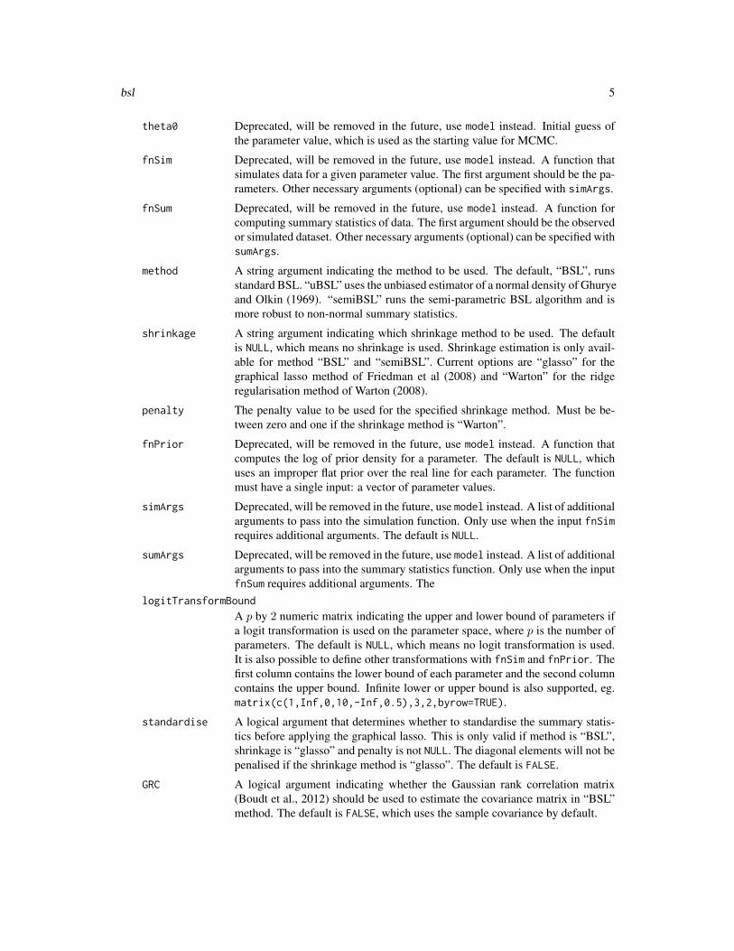
theta0 Deprecated, will be removed in the future, use model instead. Initial guess ofthe parameter value, which is used as the starting value for MCMC.

fnSim Deprecated, will be removed in the future, use model instead. A function thatsimulates data for a given parameter value. The first argument should be the pa-rameters. Other necessary arguments (optional) can be specified with simArgs.

fnSum Deprecated, will be removed in the future, use model instead. A function forcomputing summary statistics of data. The first argument should be the observedor simulated dataset. Other necessary arguments (optional) can be specified withsumArgs.

method A string argument indicating the method to be used. The default, “BSL”, runsstandard BSL. “uBSL” uses the unbiased estimator of a normal density of Ghuryeand Olkin (1969). “semiBSL” runs the semi-parametric BSL algorithm and ismore robust to non-normal summary statistics.

shrinkage A string argument indicating which shrinkage method to be used. The defaultis NULL, which means no shrinkage is used. Shrinkage estimation is only avail-able for method “BSL” and “semiBSL”. Current options are “glasso” for thegraphical lasso method of Friedman et al (2008) and “Warton” for the ridgeregularisation method of Warton (2008).

penalty The penalty value to be used for the specified shrinkage method. Must be be-tween zero and one if the shrinkage method is “Warton”.

fnPrior Deprecated, will be removed in the future, use model instead. A function thatcomputes the log of prior density for a parameter. The default is NULL, whichuses an improper flat prior over the real line for each parameter. The functionmust have a single input: a vector of parameter values.

simArgs Deprecated, will be removed in the future, use model instead. A list of additionalarguments to pass into the simulation function. Only use when the input fnSimrequires additional arguments. The default is NULL.

sumArgs Deprecated, will be removed in the future, use model instead. A list of additionalarguments to pass into the summary statistics function. Only use when the inputfnSum requires additional arguments. The

logitTransformBound

A p by 2 numeric matrix indicating the upper and lower bound of parameters ifa logit transformation is used on the parameter space, where p is the number ofparameters. The default is NULL, which means no logit transformation is used.It is also possible to define other transformations with fnSim and fnPrior. Thefirst column contains the lower bound of each parameter and the second columncontains the upper bound. Infinite lower or upper bound is also supported, eg.matrix(c(1,Inf,0,10,-Inf,0.5),3,2,byrow=TRUE).

standardise A logical argument that determines whether to standardise the summary statis-tics before applying the graphical lasso. This is only valid if method is “BSL”,shrinkage is “glasso” and penalty is not NULL. The diagonal elements will not bepenalised if the shrinkage method is “glasso”. The default is FALSE.

GRC A logical argument indicating whether the Gaussian rank correlation matrix(Boudt et al., 2012) should be used to estimate the covariance matrix in “BSL”method. The default is FALSE, which uses the sample covariance by default.

6 bsl

parallel A logical value indicating whether parallel computing should be used for sim-ulation and summary statistic evaluation. The default is FALSE. When modelsimulation is fast, it may be preferable to perform serial computations to avoidsignificant communication overhead between workers.

parallelArgs A list of additional arguments to pass into the foreach function. Only usedwhen parallel computing is enabled, default is NULL.

thetaNames Deprecated, will be removed in the future, use model instead. A string vectorof parameter names, which must have the same length as the parameter vector.The default is NULL.

plotOnTheFly A logical or numeric argument defining whether or by how many iterations aposterior figure will be plotted during running. If TRUE, a plot of approximateunivariate posteriors based on the current accepted samples will be shown byevery one thousand iterations. The default is FALSE.

verbose A logical argument indicating whether the iteration numbers (1:M) and acceptedproposal flags should be printed to track progress. The default is FALSE.

Value

An object of class bsl is returned, containing the following components:

• theta: MCMC samples from the joint approximate posterior distribution of the parameters.

• loglike: Accepted MCMC samples of the estimated log-likelihood values.

• call: The original code that was used to call the method.

• model: The “BSLMODEL” object.

• acceptanceRate: The acceptance rate of the MCMC algorithm.

• earlyRejectionRate: The early rejection rate of the algorithm (early rejection may occurwhen using bounded prior distributions).

• errorRate: The error rate. If any infinite summary statistic or positive infinite loglike occursduring the process, it is marked as an error and the proposed parameter will be rejected.

• y: The input observed data.

• n: The number of simulations from the model per MCMC iteration.

• M: The number of MCMC iterations.

• covRandWalk: The covariance matrix used in multivariate normal random walk proposals.

• method: The string argument indicating the used method.

• shrinkage: The string argument indicating the shrinkage method.

• penalty: The penalty value.

• standardise: Logical, whether to standardise the summary statistics.

• GRC: Logical, if Gaussian rank correlation matrix is used.

• logitTransform: Logical, whether a logit transformation is used in the algorithm.

• logitTransformBound: The matrix of logitTransformBound.

• parallel: Logical, whether parallel computing is used in the process.

• parallelArgs: The list of additional arguments to pass into the foreach function.

• time: The running time of class difftime.

bsl-class 7

Author(s)


References



An, Z., Nott, D. J. & Drovandi, C. (2018). Robust Bayesian Synthetic Likelihood via a Semi-Parametric Approach. ArXiv Preprint https://arxiv.org/abs/1809.05800

Friedman J, Hastie T, & Tibshirani R. (2008). Sparse inverse covariance estimation with the graph-ical lasso. Biostatistics. https://doi.org/10.1093/biostatistics/kxm045


Ghurye, S. G., & Olkin, I. (1969). Unbiased estimation of some multivariate probability densitiesand related functions. The Annals of Mathematical Statistics. https://projecteuclid.org/euclid.aoms/1177697501

Boudt, K., Cornelissen, J., and Croux, C. (2012). The Gaussian rank correlation estimator: robust-ness properties. Statistics and Computing, 22(2):471-483.

See Also

ma2, cell and mgnk for examples. selectPenalty for a function to tune the BSLasso tuningparameter and plot for functions related to visualisation.

bsl-class S4 class “bsl”.

Description

The result from function bsl is saved as class “BSL”.

Summarise a “bsl” class object.

Plot the univariate marginal posterior plot of a “bsl” class object.

Usage

## S4 method for signature 'bsl'show(object)

summary(object, ...)

https://doi.org/10.1080/10618600.2017.1302882

https://doi.org/10.1080/10618600.2018.1537928

https://doi.org/10.1080/10618600.2018.1537928



https://doi.org/10.1198/016214508000000021

https://doi.org/10.1198/016214508000000021

https://projecteuclid.org/euclid.aoms/1177697501


8 bsl-class

## S4 method for signature 'bsl'summary(object, thetaNames = NULL)

plot(x, y, ...)

## S4 method for signature 'bsl,missing'plot(x, which = 1L, thin = 1,thetaTrue = NULL, options.plot = NULL,top = "Approximate Univariate Posteriors", options.density = list(),options.theme = list())

Arguments

object A “bsl” class object to be displayed.

... Other arguments.

thetaNames Parameter names to be shown in the summary table. If not given, parameternames of the “bsl” object will be used by default.

x A “bsl” class object to plot.

y Ignore.

which An integer argument indicating which plot function to be used. The default, 1L,uses the plain plot to visualise the result. 2L uses ggplot2 to draw the plot.

thin A numeric argument indicating the gap between samples to be taken when thin-ning the MCMC draws. The default is 1, which means no thinning is used.

thetaTrue A set of values to be included on the plots as a reference line. The default isNULL.

options.plot A list of additional arguments to pass into the plot function. Only use whenwhich is 1L.

top A character argument of the combined plot title if which is 2L.options.density

A list of additional arguments to pass into the geom_density function. Only usewhen which is 2L.

options.theme A list of additional arguments to pass into the theme function. Only use whenwhich is 2L.

Value

A vector of the number of simulations per iteration, acceptance rate of the Markov chain annd scaledeffective sample size for each parameter.

Methods (by generic)

• show: Display the basic information of a “bsl” object. See show.bsl.

• summary: Summarise a bsl class object. See summary.bsl.

• plot: Plot the univariate marginal posterior plot of a “bsl” class object. See plot.bsl.

bsl-class 9

Slots

theta Object of class “matrix”. MCMC samples from the joint approximate posterior distributionof the parameters.

loglike Object of class “numeric”. Accepted MCMC samples of the estimated log-likelihoodvalues.

call Object of class “call”. The original code that was used to call the method.

model Object of class “BSLMODEL”.

acceptanceRate Object of class “numeric”. The acceptance rate of the MCMC algorithm.

earlyRejectionRate Object of class “numeric”. The early rejection rate of the algorithm (earlyrejection may occur when using bounded prior distributions).

errorRate Object of class “numeric”. The error rate. If any infinite summary statistic or positiveinfinite loglike occurs during the process, it is marked as an error and the proposed parameterwill be rejected.

y Object of class “ANY”. The observed data.

n Object of class “numeric”. The number of simulations from the model per MCMC iteration.

M Object of class “numeric”. The number of MCMC iterations.

covRandWalk Object of class “matrix”. The covariance matrix used in multivariate normal randomwalk proposals.

method Object of class “character”. The character argument indicating the used method.

shrinkage Object of class “characterOrNULL”. The character argument indicating the shrinkagemethod.

penalty Object of class “numericOrNULL”. The penalty value.

GRC Object of class “logical”. Whether the Gaussian rank correlation matrix is used.

logitTransform Object of class “logical”. The logical argument indicating whether a logit trans-formation is used in the algorithm.

logitTransformBound Object of class “matrixOrNULL”. The matrix of logitTransformBound.

standardise Object of class “logical”. The logical argument that determines whether to standard-ise the summary statistics.

parallel Object of class “logical”. The logical value indicating whether parallel computing isused in the process.

parallelArgs Object of class “listOrNULL”. The list of additional arguments to pass into theforeach function.

time Object of class “difftime”. The running time.

10 BSLMODEL-class

BSLMODEL-class S4 class “BSLMODEL”

Description

The S4 class contains the simulation and summary statistics function and other necessary argumentsfor a model to run in the main bsl function.

BSLModel is the constructor function for a BSLMODEL object.

initialize.BSLMODEL initialises a “BSLMODEL” object.

validBSLModelObject check the validity of a “BSLMODEL” object.

Usage

BSLModel(fnSim, fnSimVec, fnSum, fnLogPrior, simArgs, sumArgs, theta0,thetaNames, test = TRUE)

initialize.BSLMODEL(.Object, fnSim, fnSimVec, simArgs, fnSum, sumArgs,fnLogPrior, theta0, thetaNames, test = TRUE)

validBSLModelObject(object)

## S4 method for signature 'BSLMODEL'fn(.Object)

## S4 method for signature 'BSLMODEL'setns(.Object)

Arguments

fnSim A function that simulates data for a given parameter value. The first argumentshould be the parameters. Other necessary arguments (optional) can be specifiedwith simArgs.

fnSimVec A vectorised function that simulates a number of datasets simultaneously for agiven parameter value. The first two arguments should be the number of simula-tions to run and parameters, respectively. Other necessary arguments (optional)can be specified with simArgs. The output must be a list of each simulationresult.

fnSum A function for computing summary statistics of data. The first argument shouldbe the observed or simulated dataset. Other necessary arguments (optional) canbe specified with sumArgs.

fnLogPrior A function that computes the log of prior density for a parameter. If this ismissing, the prior by default is an improper flat prior over the real line for eachparameter. The function must have a single input: a vector of parameter values.

simArgs A list of additional arguments to pass into the simulation function. Only usewhen the input fnSim requires additional arguments.

BSLMODEL-class 11

sumArgs A list of additional arguments to pass into the summary statistics function. Onlyuse when the input fnSum requires additional arguments.

theta0 Initial guess of the parameter value.thetaNames A string vector of parameter names, which must have the same length as the

parameter vector.test Logical, whether a short simulation test will be ran upon initialisation..Object A “BSLMODEL” object.object A “BSLMODEL” object.

Methods (by generic)

• fn: Generate the generic simulation and summary statistics function for n simulations andfixed theta (for internal use).

• setns: Find and set the length of summary statistics with a test run (for internal use).

Slots

fnSim A function that simulates data for a given parameter value. The first argument should be theparameters. Other necessary arguments (optional) can be specified with simArgs.

fnSimVec A vectorised function that simulates a number of datasets simultaneously for a givenparameter value. If this is not NULL, vectorised simulation function will be used instead offnSim. The first two arguments should be the number of simulations to run and parameters,respectively. Other necessary arguments (optional) can be specified with simArgs. The outputmust be a list of each simulation result.

fnSum A function for computing summary statistics of data. The first argument should be theobserved or simulated dataset. Other necessary arguments (optional) can be specified withsumArgs. The users should code this function carefully so the output have fixed length andnever contain any Inf value.

fnLogPrior A function that computes the log of prior density for a parameter. The default is NULL,which uses an improper flat prior over the real line for each parameter. The function musthave a single input: a vector of parameter values.

simArgs A list of additional arguments to pass into the simulation function. Only use when theinput fnSim or fnSimVec requires additional arguments. The default is NULL.

sumArgs A list of additional arguments to pass into the summary statistics function. Only use whenthe input fnSum requires additional arguments. The default is NULL.

theta0 Initial guess of the parameter value, which is used as the starting value for MCMC.thetaNames Expression, parameter names.ns The number of summary statistics of a single observation. Note this will be generated automat-

ically, thus is not required for initialisation.test Logical indicator of whether a short simulation test will be ran upon initialisation.

Examples

data(ma2)model <- BSLModel(fnSim = ma2_sim, fnSum = ma2_sum, simArgs = ma2$sim_options, theta0 = ma2$start,

fnLogPrior = ma2_logPrior)validObject(model)

12 cell

cell Cell biology example

Description

This example estimates the probabilities of cell motility and cell proliferation for a discrete-timestochastic model of cell spreading. We provide the data and tuning parameters required to reproducethe results in An et al. (2019).

Usage

cell_sim(theta, Yinit, rows, cols, sim_iters, num_obs)

cell_sum(Y, Yinit)

cell_prior(theta)

cell_logPrior(theta)

Arguments

theta A vector of proposed model parameters, Pm and Pp.

Yinit The initial matrix of cell presences of size rows by cols.

rows The number of rows in the lattice (rows in the cell location matrix).

cols The number of columns in the lattice (columns in the cell location matrix).

sim_iters The number of discretisation steps to get to when an observation is actuallytaken. For example, if observations are taken every 5 minutes but the dis-cretisation level is 2.5 minutes, then sim_iters would be 2. Larger values ofsim_iters lead to more “accurate” simulations from the model, but they alsoincrease the simulation time.

num_obs The total number of images taken after initialisation.

Y A rows by cols by num_obs array of the cell presences at times 1:num_obs (nottime 0).

Details

Cell motility (movement) and proliferation (reproduction) cause tumors to spread and wounds toheal. If we can measure cell proliferation and cell motility under different situations, then we maybe able to use this information to determine the efficacy of different medical treatments.

A common method for measuring in vitro cell movement and proliferation is the scratch assay.Cells form a layer on an assay and, once they are completely covering the assay, a scratch is madeto separate the cells. Images of the cells are taken until the scratch has closed up and the cells are incontact again. Each image can be converted to a binary matrix by forming a lattice and recordingthe binary matrix (of size rows x cols) of cell presences.

cell 13

The model that we consider is a random walk model with parameters for the probability of cellmovement (Pm) and the probability of cell proliferation (Pp) and it has no tractable likelihoodfunction. We use the uninformative priors Pm U(0, 1) and Pp U(0, 1).

We have a total of 145 summary statistics, which are made up of the Hamming distances betweenthe binary matrices for each time point and the total number of cells at the final time.

Details about the types of cells that this model is suitable for and other information can be found inPrice et al. (2018) and An et al. (2019). Johnston et al. (2014) use a different ABC method anddifferent summary statistics for a similar example.

A simulated dataset

An example “observed” dataset and the tuning parameters relevant to that example can be obtainedusing data(cell). This “observed” data is a simulated dataset with Pm = 0.35 and Pp = 0.001.The lattice has 27 rows and 36 cols and there are num_obs = 144 observations after time 0 (tomimic images being taken every 5 minutes for 12 hours). The simulation is based on there initiallybeing 110 cells in the assay.

Further information about the specific choices of tuning parameters used in BSL and BSLasso canbe found in An et al. (2019).

• data: The rows x cols x num_obs array of the cell presences at times 1:144.

• sim_options: Values of sim_options relevant to this example.

• sum_options: Values of sum_options relevant to this example, i.e. just the value of Yinit.

• start: A vector of suitable initial values of the parameters for MCMC.

• cov: The covariance matrix of a multivariate normal random walk proposal distribution usedin the MCMC, in the form of a 2 by 2 matrix

Author(s)


References


Johnston, S., Simpson, M. J., McElwain, D. L. S., Binder, B. J. & Ross, J. V. (2014). Interpret-ing Scratch Assays Using Pair Density Dynamic and Approximate Bayesian Computation. OpenBiology, 4, 1-11.


Examples

require(doParallel) # You can use a different package to set up the parallel backend

# Loading the data for this example

https://doi.org/10.1080/10618600.2018.1537928

https://doi.org/10.1080/10618600.2018.1537928

https://doi.org/10.1080/10618600.2017.1302882

14 cell

data(cell)model <- BSLModel(fnSim = cell_sim, fnSum = cell_sum, simArgs = cell$sim_options,

sumArgs = cell$sum_options, theta0 = cell$start, fnLogPrior = cell_logPrior,thetaNames = expression(P[m], P[p]))

true_cell <- c(0.35, 0.001)

# Performing BSL (reduce the number of iterations M if desired)# Opening up the parallel pools using doParallelcl <- makeCluster(detectCores() - 1)registerDoParallel(cl)resultCellBSL <- bsl(cell$data, n = 5000, M = 10000, model = model, covRandWalk = cell$cov,

parallel = TRUE, verbose = TRUE)stopCluster(cl)registerDoSEQ()show(resultCellBSL)summary(resultCellBSL)plot(resultCellBSL, thetaTrue = true_cell, thin = 20)

# Performing uBSL (reduce the number of iterations M if desired)# Opening up the parallel pools using doParallelcl <- makeCluster(detectCores() - 1)registerDoParallel(cl)resultCelluBSL <- bsl(cell$data, n = 5000, M = 10000, model = model, covRandWalk = cell$cov,

method = 'uBSL', parallel = TRUE, verbose = TRUE)stopCluster(cl)registerDoSEQ()show(resultCelluBSL)summary(resultCelluBSL)plot(resultCelluBSL, thetaTrue = true_cell, thin = 20)

# Performing tuning for BSLassossy <- cell_sum(cell$data, cell$sum_options$Yinit)lambda_all <- list(exp(seq(0.5,2.5,length.out=20)), exp(seq(0,2,length.out=20)),

exp(seq(-1,1,length.out=20)), exp(seq(-1,1,length.out=20)))# Opening up the parallel pools using doParallelcl <- makeCluster(detectCores() - 1)registerDoParallel(cl)set.seed(100)sp_cell <- selectPenalty(ssy, n = c(500, 1000, 1500, 2000), lambda_all, theta = true_cell,

M = 100, sigma = 1.5, model = model, method = 'BSL', shrinkage = 'glasso',parallelSim = TRUE, parallelMain = FALSE)

stopCluster(cl)registerDoSEQ()sp_cellplot(sp_cell)

# Performing BSLasso with a fixed penalty (reduce the number of iterations M if desired)# Opening up the parallel pools using doParallelcl <- makeCluster(detectCores() - 1)registerDoParallel(cl)resultCellBSLasso <- bsl(cell$data, n = 1500, M = 10000, theta0 = cell$start,

covRandWalk = cell$cov, fnSim = cell_sim, fnSum = cell_sum,shrinkage = 'glasso', penalty = 1.3, fnPrior = cell_prior,

combinePlotsBSL 15

simArgs = cell$sim_options, sumArgs = cell$sum_options,parallel = TRUE, parallelArgs = list(.packages = 'BSL'),thetaNames = expression(P[m], P[p]), verbose = TRUE)

stopCluster(cl)registerDoSEQ()show(resultCellBSLasso)summary(resultCellBSLasso)plot(resultCellBSLasso, thetaTrue = true_cell, thin = 20)

# Performing semiBSL (reduce the number of iterations M if desired)# Opening up the parallel pools using doParallelcl <- makeCluster(detectCores() - 1)registerDoParallel(cl)resultCellSemiBSL <- bsl(cell$data, n = 5000, M = 10000, theta0 = cell$start,

covRandWalk = cell$cov, fnSim = cell_sim, fnSum = cell_sum,method = 'semiBSL', fnPrior = cell_prior,simArgs = cell$sim_options, sumArgs = cell$sum_options,parallel = TRUE, parallelArgs = list(.packages = 'BSL'),thetaNames = expression(P[m], P[p]), verbose = TRUE)

stopCluster(cl)registerDoSEQ()show(resultCellSemiBSL)summary(resultCellSemiBSL)plot(resultCellSemiBSL, thetaTrue = true_cell, thin = 20)

# Plotting the results together for comparison# plot using the R default plot functionpar(mar = c(5, 4, 1, 2), oma = c(0, 1, 2, 0))combinePlotsBSL(list(resultCellBSL, resultCelluBSL, resultCellBSLasso, resultCellSemiBSL),

which = 1, thetaTrue = true_cell, thin = 20, label = c('bsl', 'ubsl', 'bslasso', 'semiBSL'),col = 1:4, lty = 1:4, lwd = 1)

mtext('Approximate Univariate Posteriors', outer = TRUE, cex = 1.5)

combinePlotsBSL Plot the densities of multiple “bsl” class objects.

Description

The function combinePlotsBSL can be used to plot multiple BSL densities together, optionallywith the true values for the parameters.

Usage

combinePlotsBSL(objectList, which = 1L, thin = 1, thetaTrue = NULL,label = NULL, legendPosition = c("auto", "right", "bottom")[1],legendNcol = NULL, col = NULL, lty = NULL, lwd = NULL,cex.lab = 1, cex.axis = 1, cex.legend = 0.75,top = "Approximate Marginal Posteriors", options.color = list(),

16 combinePlotsBSL

options.linetype = list(), options.size = list(),options.theme = list())

Arguments

objectList A list of “bsl” class objects.which An integer argument indicating which plot function to be used. The default, 1L,

uses the plain plot to visualise the result. 2L uses ggplot2 to draw the plot.thin A numeric argument indicating the gap between samples to be taken when thin-

ning the MCMC draws. The default is 1, which means no thinning is used.thetaTrue A set of values to be included on the plots as a reference line. The default is

NULL.label A string vector indicating the labels to be shown in the plot legend. The default

is NULL, which uses the names from objectList.legendPosition One of the three string arguments, “auto”, “right” or “bottom”, indicating the

legend position. The default is “auto”, which automatically choose from “right”and “bottom”. Only used when which is 1L.

legendNcol A integer argument indicating the number of columns of the legend. The default,NULL, put all legends in the same row or column depending on legendPosition.Only used when which is 1L.

col A vector argument containing the plotting color for each density curve. Eachelement of the vector will be passed into lines. Only used when which is 1L.

lty A vector argument containing the line type for each density curve. Each elementof the vector will be passed into lines. Only used when which is 1L.

lwd A vector argument containing the line width for each density curve. Each ele-ment of the vector will be passed into lines. Only used when which is 1L.

cex.lab The magnification to be used for x and y labels relative to the current setting ofcex. To be passed into plot. Only used when which is 1L.

cex.axis The magnification to be used for axis annotation relative to the current settingof cex. To be passed into plot. Only used when which is 1L.

cex.legend The magnification to be used for legend annotation relative to the current settingof cex. Only used when which is 1L.

top A string argument of the combined plot title. Only used when which is 2L.options.color A list of additional arguments to pass into function ggplot2::scale_color_manual.

Only used when which is 2L.options.linetype

A list of additional arguments to pass into function ggplot2::scale_linetype_manual.Only used when which is 2L.

options.size A list of additional arguments to pass into function ggplot2::scale_size_manual.Only used when which is 2L.


See Also

ma2 for an example

cor2cov 17

cor2cov Convert a correlation matrix to a covariance matrix

Description

This function converts a correlation matrix to a covariance matrix

Usage

cor2cov(corr, std)

Arguments

corr The correlation matrix to be converted. This must be symmetric.

std A vector that contains the standard deviations of the variables in the correlationmatrix.

Value

The covariance matrix.

fn Functions to be used in bsl (for internal use)

Description

Generate the generic simulation and summary statistics function for n simulations and fixed theta(for internal use).

Usage

fn(.Object)

Arguments

.Object A “BSLMODEL” object.

18 gaussianRankCorr

gaussianRankCorr Gaussian rank correlation

Description

This function computes the Gaussian rank correlation of Boudt et al. (2012).

Usage

gaussianRankCorr(x, vec = FALSE)

Arguments

x A numeric matrix representing data where the number of rows is the number ofindependent data points and the number of columns are the number of variablesin the dataset.

vec A logical argument indicating if the vector of correlations should be returnedinstead of a matrix.

Value

Gaussian rank correlation matrix (default) or a vector of pair correlations.

References

Boudt, K., Cornelissen, J., and Croux, C. (2012). The Gaussian rank correlation estimator: robust-ness properties. Statistics and Computing, 22(2):471-483.

See Also

cor2cov for converting a correlation matrix to a covariance matrix.

Examples

data(ma2)set.seed(100)

# generate 1000 simualtions from the ma2 simulation functionx <- t(replicate(1000, ma2_sim(ma2$start, 10)))

corr1 <- cor(x) # traditional correlation matrixcorr2 <- gaussianRankCorr(x) # Gaussian rank correlation matrixpar(mfrow = c(1, 2))image(corr1, main = 'traditional correlation matrix')image(corr2, main = 'Gaussian rank correlation matrix')

std <- apply(x, MARGIN = 2, FUN = sd) # standard deviationscor2cov(gaussianRankCorr(x), std) # convert to covariance matrix

gaussianSynLike 19

gaussianSynLike Estimating the Gaussian synthetic likelihood

Description

This function estimates the Gaussian synthetic likelihood function of Wood (2010). Shrinkage onthe Gaussian covariance matrix is also available (see An et al 2019).

Usage

gaussianSynLike(ssy, ssx, shrinkage = NULL, penalty = NULL,standardise = FALSE, GRC = FALSE, log = TRUE, verbose = FALSE)

Arguments

ssy The observed summary statisic.

ssx A matrix of the simulated summary statistics. The number of rows is the sameas the number of simulations per iteration.

shrinkage A string argument indicating which shrinkage method to be used. The defaultis NULL, which means no shrinkage is used. Shrinkage estimation is only avail-able for method “BSL” and “semiBSL”. Current options are “glasso” for thegraphical lasso method of Friedman et al (2008) and “Warton” for the ridgeregularisation method of Warton (2008).




log A logical argument indicating if the log of likelihood is given as the result. Thedefault is TRUE.

verbose A logical argument indicating whether an error message should be printed if thefunction fails to compute a likelihood. The default is FALSE.

Value

The estimated synthetic (log) likelihood value.

20 gaussianSynLikeGhuryeOlkin

References





See Also

gaussianSynLikeGhuryeOlkin for the unbiased synthetic likelihood estimator, semiparaKernelEstimatefor the semi-parametric likelihood estimator.

Examples

data(ma2)y <- ma2$data # the observed data

theta_true <- c(0.6, 0.2)x <- matrix(0, 300, 50)set.seed(100)for(i in 1:300) x[i, ] <- ma2_sim(theta_true, 50)

# the standard Gaussian synthetic likelihood (the likelihood estimator used in BSL)gaussianSynLike(y, x)# the Gaussian synthetic likelihood with glasso shrinkage estimation# (the likelihood estimator used in BSLasso)gaussianSynLike(y, x, shrinkage = 'glasso', penalty = 0.1)# the Gaussian synthetic likelihood with Warton shrinkage estimationgaussianSynLike(y, x, shrinkage = 'Warton', penalty = 0.9)

gaussianSynLikeGhuryeOlkin

Estimating the Gaussian synthetic likelihood with an unbiased estima-tor

Description

This function computes an unbiased, nonnegative estimate of a normal density function from simu-lations assumed to be drawn from it. See Price et al. (2018) and Ghurye and Olkin (1969).

https://doi.org/10.1080/10618600.2017.1302882

https://doi.org/10.1080/10618600.2018.1537928

https://doi.org/10.1080/10618600.2018.1537928


https://doi.org/10.1198/016214508000000021

https://doi.org/10.1198/016214508000000021

gaussianSynLikeGhuryeOlkin 21

Usage

gaussianSynLikeGhuryeOlkin(ssy, ssx, log = TRUE, verbose = FALSE)

Arguments

ssy The observed summary statisic.


log A logical argument indicating if the log of likelihood is given as the result. Thedefault is TRUE.

verbose A logical argument indicating whether an error message should be printed if thefunction fails to compute a likelihood. The default is FALSE.

Value


References


Ghurye, S. G., & Olkin, I. (1969). Unbiased estimation of some multivariate probability densitiesand related functions. The Annals of Mathematical Statistics. https://projecteuclid.org/euclid.aoms/1177697501

See Also

gaussianSynLike for the standard synthetic likelihood estimator, semiparaKernelEstimate forthe semi-parametric likelihood estimator.

Examples



# unbiased estimate of the Gaussian synthetic likelihood# (the likelihood estimator used in uBSL)gaussianSynLikeGhuryeOlkin(y, x)

https://doi.org/10.1080/10618600.2017.1302882



22 ma2

ma2 An MA(2) model

Description

In this example we wish to estimate the parameters of a simple MA(2) time series model. Weprovide the data and tuning parameters required to reproduce the results in An et al. (2019).

Usage

data(ma2)

ma2_sim(theta, T)

ma2_sum(x)

ma2_prior(theta)

ma2_logPrior(theta)

Arguments

theta A vector of proposed model parameters, θ1 and θ2.T The number of observations.x Observed or simulated data in the format of a vector of length T .

Details

This example is based on estimating the parameters of a basic MA(2) time series model of the form

yt = zt + θ1zt−1 + θ2zt−2,

where t = 1, . . . , T and zt N(0, 1) for t = −1, 0, . . . , T . A uniform prior is used for this example,subject to the restrictions that −2 < θ1 < 2, θ1 + θ2 > −1 and θ1 − θ2 < 1 so that invertibility ofthe time series is satisfied. The summary statistics are simply the full data.

A simulated dataset

An example “observed” dataset and the tuning parameters relevant to that example can be obtainedusing data(ma2). This “observed” data is a simulated dataset with θ1 = 0.6, θ2 = 0.2 and T = 50.Further information about this model and the specific choices of tuning parameters used in BSL andBSLasso can be found in An et al. (2019).

• data: A time series dataset, in the form of a vector of length T• sim_options: A list containing T = 50

• start: A vector of suitable initial values of the parameters for MCMC• cov: The covariance matrix of a multivariate normal random walk proposal distribution used

in the MCMC, in the form of a 2 by 2 matrix

ma2 23

Author(s)


References


Examples

## Not run:# Loading the data for this exampledata(ma2)model <- BSLModel(fnSim = ma2_sim, fnSum = ma2_sum, simArgs = ma2$sim_options, theta0 = ma2$start,

fnLogPrior = ma2_logPrior)true_ma2 <- c(0.6,0.2)

# Performing BSL (reduce the number of iterations M if desired)resultMa2BSL <- bsl(y = ma2$data, n = 500, M = 300000, model = model, covRandWalk = ma2$cov,

method = 'BSL', verbose = TRUE)show(resultMa2BSL)summary(resultMa2BSL)plot(resultMa2BSL, which = 1, thetaTrue = true_ma2, thin = 20)

# Performing uBSL (reduce the number of iterations M if desired)resultMa2uBSL <- bsl(y = ma2$data, n = 500, M = 300000, model = model, covRandWalk=ma2$cov,

method = 'uBSL', verbose = TRUE)show(resultMa2uBSL)summary(resultMa2uBSL)plot(resultMa2uBSL, which = 1, thetaTrue = true_ma2, thin = 20)

# Performing tuning for BSLassossy <- ma2_sum(ma2$data)lambda_all <- list(exp(seq(-3,0.5,length.out=20)), exp(seq(-4,-0.5,length.out=20)),

exp(seq(-5.5,-1.5,length.out=20)), exp(seq(-7,-2,length.out=20)))set.seed(100)sp_ma2 <- selectPenalty(ssy = ssy, n = c(50, 150, 300, 500), lambda_all, theta = true_ma2,

M = 100, sigma = 1.5, model = model, method = 'BSL', shrinkage = 'glasso')sp_ma2plot(sp_ma2)

# Performing BSLasso with a fixed penalty (reduce the number of iterations M if desired)resultMa2BSLasso <- bsl(y = ma2$data, n = 300, M = 250000, model = model, covRandWalk=ma2$cov,

method = 'BSL', shrinkage = 'glasso', penalty = 0.027, verbose = TRUE)show(resultMa2BSLasso)summary(resultMa2BSLasso)plot(resultMa2BSLasso, which = 1, thetaTrue = true_ma2, thin = 20)

# Performing semiBSL (reduce the number of iterations M if desired)resultMa2SemiBSL <- bsl(y = ma2$data, n = 500, M = 300000, model = model, covRandWalk=ma2$cov,

https://doi.org/10.1080/10618600.2018.1537928

https://doi.org/10.1080/10618600.2018.1537928

24 mgnk

method = 'semiBSL', verbose = TRUE)show(resultMa2SemiBSL)summary(resultMa2SemiBSL)plot(resultMa2SemiBSL, which = 1, thetaTrue = true_ma2, thin = 20)

# Plotting the results together for comparison# plot using the R default plot functionpar(mar = c(5, 4, 1, 2), oma = c(0, 1, 2, 0))combinePlotsBSL(list(resultMa2BSL, resultMa2uBSL, resultMa2BSLasso, resultMa2SemiBSL), which = 1,

thetaTrue = true_ma2, thin = 20, label = c('bsl', 'uBSL', 'bslasso', 'semiBSL'),col = c('black', 'red', 'blue', 'green'), lty = 1:4, lwd = 1)

mtext('Approximate Univariate Posteriors', outer = TRUE, cex = 1.5)

# plot using the ggplot2 packagecombinePlotsBSL(list(resultMa2BSL, resultMa2uBSL, resultMa2BSLasso, resultMa2SemiBSL), which = 2,

thetaTrue = true_ma2, thin = 20, label = c('bsl', 'ubsl', 'bslasso', 'semiBSL'),options.color = list(values=c('black', 'red', 'blue', 'green')),options.linetype = list(values = 1:4), options.size = list(values = rep(1, 4)),options.theme = list(plot.margin = grid::unit(rep(0.03,4), 'npc'),

axis.title = ggplot2::element_text(size=12), axis.text = ggplot2::element_text(size = 8),legend.text = ggplot2::element_text(size = 12)))

## End(Not run)

mgnk The multivariate G&K example

Description

Here we provide the data and tuning parameters required to reproduce the results from the multi-variate G & K (Drovandi and Pettitt, 2011) example from An et al. (2019).

Usage

mgnk_sim(theta_tilde, T, J, bound)

mgnk_sum(y)

Arguments

theta_tilde A vector with 15 elements for the proposed model parameters.

T The number of observations in the data.

J The number of variables in the data.

bound A matrix of boundaries for the uniform prior.

y A T x J matrix of data.

mgnk 25

Details

It is not practical to give a reasonable explanation of this example through R documentation giventhe number of equations involved. We refer the reader to the BSLasso paper (An et al., 2019)at https://doi.org/10.1080/10618600.2018.1537928 for information on the model and sum-mary statistic used in this example.

An example dataset

We use the foreign currency exchange data available from http://www.rba.gov.au/statistics/historical-data.html as in An et al. (2019).

• data: A 1651 by 3 matrix of data.

• sim_options: Values of sim_options relevant to this example.

• start: A vector of suitable initial values of the parameters for MCMC.

• cov: The covariance matrix of a multivariate normal random walk proposal distribution usedin the MCMC, in the form of a 15 by 15 matrix

Author(s)


References


Drovandi, C. C. and Pettitt, A. N. (2011). Likelihood-free Bayesian estimation of multivariatequantile distributions. Computational Statistics and Data Analysis. https://doi.org/10.1016/j.csda.2011.03.019

Examples

require(doParallel) # You can use a different package to set up the parallel backendrequire(MASS)require(elliplot)

# Loading the data for this exampledata(mgnk)model <- BSLModel(fnSim = mgnk_sim, fnSum = mgnk_sum, simArgs = mgnk$sim_options,

theta0 = mgnk$start, thetaNames = expression(a[1],b[1],g[1],k[1],a[2],b[2],g[2],k[2],a[3],b[3],g[3],k[3],delta[12],delta[13],delta[23]))

# Performing BSL (reduce the number of iterations M if desired)# Opening up the parallel pools using doParallelcl <- makeCluster(detectCores() - 1)registerDoParallel(cl)resultMgnkBSL <- bsl(mgnk$data, n = 60, M = 80000, model = model, covRandWalk = mgnk$cov,

method = 'BSL', parallel = TRUE, parallelArgs = list(.packages='MASS',.export='ninenum'),

https://doi.org/10.1080/10618600.2018.1537928

http://www.rba.gov.au/statistics/historical-data.html

http://www.rba.gov.au/statistics/historical-data.html

https://doi.org/10.1080/10618600.2018.1537928

https://doi.org/10.1080/10618600.2018.1537928

https://doi.org/10.1016/j.csda.2011.03.019

https://doi.org/10.1016/j.csda.2011.03.019

26 mgnk

verbose = TRUE)stopCluster(cl)registerDoSEQ()show(resultMgnkBSL)summary(resultMgnkBSL)plot(resultMgnkBSL, which = 2, thin = 20)

# Performing uBSL (reduce the number of iterations M if desired)# Opening up the parallel pools using doParallelcl <- makeCluster(detectCores() - 1)registerDoParallel(cl)resultMgnkuBSL <- bsl(mgnk$data, n = 60, M = 80000, model = model, covRandWalk = mgnk$cov,

method = 'uBSL', parallel = TRUE, parallelArgs = list(.packages='MASS',.export='ninenum'),verbose = TRUE)

stopCluster(cl)registerDoSEQ()show(resultMgnkuBSL)summary(resultMgnkuBSL)plot(resultMgnkuBSL, which = 2, thin = 20)

# Performing tuning for BSLassossy <- mgnk_sum(mgnk$data)lambda_all <- list(exp(seq(-2.5,0.5,length.out=20)), exp(seq(-2.5,0.5,length.out=20)),

exp(seq(-4,-0.5,length.out=20)), exp(seq(-5,-2,length.out=20)))

# Opening up the parallel pools using doParallelcl <- makeCluster(detectCores() - 1)registerDoParallel(cl)set.seed(100)sp_mgnk <- selectPenalty(ssy, n = c(15, 20, 30, 50), lambda_all = lambda_all, theta = mgnk$start,

M = 100, sigma = 1.5, model = model, method = 'BSL', shrinkage = 'glasso', standardise = TRUE,parallelSim = TRUE, parallelSimArgs = list(.packages = 'MASS', .export = 'ninenum'),parallelMain = TRUE)

stopCluster(cl)registerDoSEQ()sp_mgnkplot(sp_mgnk)

# Performing BSLasso with a fixed penalty (reduce the number of iterations M if desired)# Opening up the parallel pools using doParallelcl <- makeCluster(detectCores() - 1)registerDoParallel(cl)resultMgnkBSLasso <- bsl(mgnk$data, n = 20, M = 80000, model = model, covRandWalk = mgnk$cov,

method = 'BSL', shrinkage = 'glasso', penalty = 0.3, standardise = TRUE, parallel = TRUE,parallelArgs = list(.packages = 'MASS', .export = 'ninenum'), verbose = TRUE)

stopCluster(cl)registerDoSEQ()show(resultMgnkBSLasso)summary(resultMgnkBSLasso)plot(resultMgnkBSLasso, which = 2, thin = 20)

penbsl 27

# Performing semiBSL (reduce the number of iterations M if desired)# Opening up the parallel pools using doParallelcl <- makeCluster(detectCores() - 1)registerDoParallel(cl)resultMgnkSemiBSL <- bsl(mgnk$data, n = 60, M = 80000, model = model, covRandWalk = mgnk$cov,

method = 'semiBSL', parallel = TRUE, parallelArgs = list(.packages='MASS',.export='ninenum'),verbose = TRUE)

stopCluster(cl)registerDoSEQ()show(resultMgnkSemiBSL)summary(resultMgnkSemiBSL)plot(resultMgnkSemiBSL, which = 2, thin = 20)

# Plotting the results together for comparison# plot using the R default plot functionpar(mar = c(4, 4, 1, 1), oma = c(0, 1, 2, 0))combinePlotsBSL(list(resultMgnkBSL, resultMgnkuBSL, resultMgnkBSLasso, resultMgnkSemiBSL),

which = 1, thin = 20, label = c('bsl', 'bslasso', 'semiBSL'), col = c('red', 'blue', 'green'),lty = 2:4, lwd = 1)

mtext('Approximate Univariate Posteriors', outer = TRUE, line = 0.75, cex = 1.2)

# plot using the ggplot2 packagecombinePlotsBSL(list(resultMgnkBSL, resultMgnkuBSL, resultMgnkBSLasso, resultMgnkSemiBSL),

which = 2, thin = 20, label=c('bsl','bslasso','semiBSL'),options.color=list(values=c('red','blue','green')),options.linetype = list(values = 2:4), options.size = list(values = rep(1, 3)),options.theme = list(plot.margin = grid::unit(rep(0.03,4),'npc'),

axis.title = ggplot2::element_text(size=12), axis.text = ggplot2::element_text(size = 8),legend.text = ggplot2::element_text(size = 12)))

penbsl S3 reference class of the result from tuning to select the optimal penaltyfor BSLasso

Description

Two functions (print and plot) are provided for class “penbsl".

Usage

## S3 method for class 'penbsl'print(x, digits = max(3L, getOption("digits") - 4L),...)

## S3 method for class 'penbsl'plot(x, logscale = TRUE, ...)

28 plot.bsl

Arguments

x A “penbsl" class object, typically the output of function selectPenalty.

digits The number of digits to print.

... Other arguments.

logscale A logical indicator whether the x-axis (penalty) should be log transformed. Thedefault is TRUE.

Author(s)


plot.bsl Plot method for class “bsl”

Description

Plot the univariate marginal posterior plot of a bsl class object.

Usage

plot.bsl(x, which = 1L, thin = 1, thetaTrue = NULL,options.plot = NULL, top = "Approximate Univariate Posteriors",options.density = list(), options.theme = list())

marginalPostDefault(x, thin = 1, thetaTrue = NULL,options.plot = NULL)

marginalPostGgplot(x, thin = 1, thetaTrue = NULL,top = "Approximate Univariate Posteriors", options.density = list(),options.theme = list())

Arguments

x A “bsl” class object to plot.

which An integer argument indicating which plot function to be used. The default,1L, uses the plain plot to visualise the result. 2L uses ggplot2 to generate anaesthetically nicer figure.

thin A numeric argument indicating the gap between samples to be taken when thin-ning the MCMC draws. The default is 1L, which means no thinning is used.

thetaTrue A set of values to be included on the plots as a reference line. The default isNULL.

options.plot A list of additional arguments to pass into the plot function. Only use whenwhich is 1L.

top A string argument of the combined plot title if which is 2L.

selectPenalty 29

options.density

A list of additional arguments to pass into the geom_density function. Only usewhen which is 2L.


Author(s)


See Also

combinePlotBSL for a function to plot multiple BSL densities.

Examples

## Not run:# pretend we had a bsl resultresult <- new('bsl')result@theta <- MASS::mvrnorm(10000, c(0.6, 0.2), diag(c(1, 1)))result@M <- 10000

# plot using the R default plot functionpar(mar = c(5, 4, 1, 2), oma = c(0, 1, 3, 0))plot(result, which = 1, thin = 10, thetaTrue = c(0.6, 0.2),

options.plot = list(cex.main = 1, col = 'red', lty = 2, lwd = 2, main = NA))mtext('Approximate Univariate Posteriors', outer = TRUE, cex = 1.5)

# plot using the ggplot2 packageplot(result, which = 2, thin = 10, thetaTrue = c(0.6, 0.2),

options.density = list(colour = 'darkblue', fill = 'grey80', size = 1),options.theme = list(plot.margin = grid::unit(rep(0.05,4), 'npc'),

axis.text = ggplot2::element_text(size = 10)))

## End(Not run)

selectPenalty Selecting BSLasso Penalty

Description

This is the main function for selecting the shrinkage (graphical lasso or Warton’s estimation) penaltyparameter for method BSL or semiBSL based on a point estimate of the parameters. Parallel com-puting is supported with the R package foreach.

30 selectPenalty

Usage

selectPenalty(ssy, n, lambda_all, M, sigma, model, theta = model@theta0,method = c("BSL", "semiBSL")[1], shrinkage = c("glasso","Warton")[1], standardise = FALSE, GRC = FALSE,parallelSim = FALSE, parallelSimArgs = NULL, parallelMain = FALSE,verbose = TRUE, fnSim, fnSum, simArgs, sumArgs)

Arguments

ssy A summary statistic vector for the observed data.

n A vector of possible values of n, the number of simulations from the model perMCMC iteration for estimating the synthetic likelihood.

lambda_all A list, with each entry containing the vector of penalty values to test for thecorresponding choice of n.

M The number of repeats to use in estimating the standard deviation of the esti-mated log synthetic likelihood.

sigma The standard deviation of the log synthetic likelihood estimator to aim for, usu-ally a value between 1 and 2. This reflects the mixing of a Markov chain.

model A “BSLMODEL” object generated with function BSLModel. See BSLModel.

theta A point estimate of the parameter value which all of the simulations will bebased on.

method A string argument indicating the method to be used. The default, “BSL”, runsBSL. “semiBSL” runs the semi-parametric BSL algorithm and is more robust tonon-normal summary statistics.

shrinkage A string argument indicating which shrinkage method to be used. Current op-tions are “glasso” for the graphical lasso method of Friedman et al (2008) and“Warton” for the ridge regularisation method of Warton (2008).



parallelSim A logical value indicating whether parallel computing should be used for simu-lation and summary statistic evaluation. Default is FALSE.

parallelSimArgs

A list of additional arguments to pass into the foreach function. Only usedwhen parallelSim is TRUE, default is NULL.

parallelMain A logical value indicating whether parallel computing should be used to com-puting the graphical lasso function. Default is FALSE.

verbose A logical argument indicating whether the iteration numbers (1:M) should beprinted to track progress. The default is FALSE.

selectPenalty 31

fnSim Deprecated, will be removed in the future, use model instead. A function thatsimulates data for a given parameter value. The first argument should be the pa-rameters. Other necessary arguments (optional) can be specified with simArgs.

fnSum Deprecated, will be removed in the future, use model instead. A function forcomputing summary statistics of data. The first argument should be the observedor simulated dataset. Other necessary arguments (optional) can be specified withsumArgs.

simArgs Deprecated, will be removed in the future, use model instead. A list of additionalarguments to pass into the simulation function. Only use when the input fnSimrequires additional arguments. The default is NULL.

sumArgs Deprecated, will be removed in the future, use model instead. A list of additionalarguments to pass into the summary statistics function. Only use when the inputfnSum requires additional arguments. The

Value

An object of class penbsl is returned, containing the following components:

• resultsDF: A data frame containing the following:

– n: The choices of n that were specified.– penalty: The choices of the penalty that were specified.– sigma: The standard deviation of the log synthetic likelihood estimator under the above

choices.– sigmaOpt: An indicator of whether it was the closest sigma to the desired one for each

choice of n.

• call: The original code that was used to call the method.

The functions print() and plot() are both available for types of class penbsl.

Author(s)


References



See Also

ma2, cell and mgnk for examples. bsl for a function to run BSLasso after selecting the tuningparameter and penbsl for functions related to visualisation.

https://doi.org/10.1080/10618600.2018.1537928

https://doi.org/10.1080/10618600.2018.1537928

https://doi.org/10.1198/016214508000000021

https://doi.org/10.1198/016214508000000021

32 semiparaKernelEstimate

semiparaKernelEstimate

Estimating the semi-parametric joint likelihood

Description

This function computes the semi-parametric likelihood estimator of An et al (2018). Kernel densityestimates are used for modelling each univariate marginal distribution, and the dependence structurebetween summaries are captured using a Gaussian copula.

Usage

semiparaKernelEstimate(ssy, ssx, kernel = "gaussian", shrinkage = NULL,penalty = NULL, log = TRUE)

Arguments

ssy The observed summary statistic.


kernel A string argument indicating the smoothing kernel to pass into density forestimating the marginal distribution of each summary statistic. Only “gaussian"and “epanechnikov" are available. The default is “gaussian".

shrinkage A string argument indicating which shrinkage method to be used on the correla-tion matrix of the Gaussian copula. The default is NULL, which means no shrink-age is used. Current options are “glasso" for graphical lasso and “Warton" forthe ridge regularisation method of Warton (2008).


log A logical argument indicating if the log of the likelihood is given as the result.The default is TRUE.

Value


References

An, Z., Nott, D. J. & Drovandi, C. (2018). Robust Bayesian Synthetic Likelihood via a Semi-Parametric Approach. https://arxiv.org/abs/1809.05800


Warton, D. I. (2008). Penalized Normal Likelihood and Ridge Regularization of Correlation andCovariance Matrices, Journal of the American Statistical Association. https://www.tandfonline.com/doi/abs/10.1198/016214508000000021



https://www.tandfonline.com/doi/abs/10.1198/016214508000000021

https://www.tandfonline.com/doi/abs/10.1198/016214508000000021

setns 33

See Also

gaussianSynLike for the standard synthetic likelihood estimator, gaussianSynLikeGhuryeOlkinfor the unbiased synthetic likelihood estimator.

Examples



# the default semi-parametric synthetic likelihood estimator of semiBSLsemiparaKernelEstimate(y, x)# using shrinkage on the correlation matrix of the Gaussian copula is also possiblesemiparaKernelEstimate(y, x, shrinkage = 'Warton', penalty = 0.6)

setns Find the length of summary statistics (for internal use)

Description

Find and set the length of summary statistics with a test run (for internal use).

Usage

setns(.Object)

Arguments

.Object A “BSLMODEL” object.

show.bsl Show method for class “bsl”. Display the basic information of a bslobject.

Description

Display the basic information of a bsl object.

Usage

show.bsl(object)

34 summary.bsl

Arguments

object A “bsl” class object.

summary.bsl Summary method for class “bsl”

Description

Summarise a bsl class object.

Usage

summary.bsl(object, thetaNames = NULL)

Arguments

object A “bsl” class object to be summarised.

thetaNames Parameter names to be shown in the summary table. Parameter names of the bslobject will be used by default.

Value

A vector of the number of simulations per iteration, acceptance rate of the Markov chain and effec-tive sample size for each parameter.

Index

BSL (BSL-package), 3bsl, 3, 4, 31bsl,bsl-method (bsl-class), 7bsl-class, 7BSL-package, 3BSLModel, 4, 30BSLModel (BSLMODEL-class), 10BSLMODEL-class, 10

cell, 3, 7, 12, 31cell_logPrior (cell), 12cell_prior (cell), 12cell_sim (cell), 12cell_sum (cell), 12combinePlotBSL, 29combinePlotsBSL, 15cor2cov, 17, 18

fn, 17fn,BSLMODEL-method (BSLMODEL-class), 10

gaussianRankCorr, 18gaussianSynLike, 19, 21, 33gaussianSynLikeGhuryeOlkin, 20, 20, 33

initialize.BSLMODEL (BSLMODEL-class), 10

ma2, 3, 7, 16, 22, 31ma2_logPrior (ma2), 22ma2_prior (ma2), 22ma2_sim (ma2), 22ma2_sum (ma2), 22marginalPostDefault (plot.bsl), 28marginalPostGgplot (plot.bsl), 28mgnk, 3, 7, 24, 31mgnk_sim (mgnk), 24mgnk_sum (mgnk), 24

new.bsl (bsl-class), 7

penbsl, 27, 31

plot, 7plot (bsl-class), 7plot,bsl,missing-method (bsl-class), 7plot.bsl, 8, 28plot.penbsl (penbsl), 27print.penbsl (penbsl), 27

selectPenalty, 3, 7, 28, 29semiparaKernelEstimate, 20, 21, 32setns, 33setns,BSLMODEL-method (BSLMODEL-class),

10show,bsl-method (bsl-class), 7show.bsl, 8, 33summary (bsl-class), 7summary,bsl-method (bsl-class), 7summary.bsl, 8, 34

validBSLModelObject (BSLMODEL-class), 10

35

Documents

Package ‘BSL’ - download.nust.na