Embed Size (px)
Citation preview
Package ‘aod’February 19, 2015
Version 1.3
Date 2012-04-10
Title Analysis of Overdispersed Data
Author Matthieu Lesnoff <[email protected]> and RenaudLancelot <[email protected]>
Maintainer Renaud Lancelot <[email protected]>
Depends R (>= 2.0.0), methods, stats
Suggests MASS, boot, lme4
Description This package provides a set of functions to analyseoverdispersed counts or proportions. Most of the methods arealready available elsewhere but are scattered in differentpackages. The proposed functions should be considered ascomplements to more sophisticated methods such as generalizedestimating equations (GEE) or generalized linear mixed effectmodels (GLMM).
License GPL (>= 2)
URL http://cran.r-project.org/package=aod
LazyData yes
Repository CRAN
Date/Publication 2012-04-10 07:30:34
NeedsCompilation no
R topics documented:aic-class . . . . . . . . . . . . . . . . . . . . . . . . . . . . . . . . . . . . . . . . . . . 2AIC-methods . . . . . . . . . . . . . . . . . . . . . . . . . . . . . . . . . . . . . . . . 3anova-methods . . . . . . . . . . . . . . . . . . . . . . . . . . . . . . . . . . . . . . . 4antibio . . . . . . . . . . . . . . . . . . . . . . . . . . . . . . . . . . . . . . . . . . . . 5aod-pkg . . . . . . . . . . . . . . . . . . . . . . . . . . . . . . . . . . . . . . . . . . . 6betabin . . . . . . . . . . . . . . . . . . . . . . . . . . . . . . . . . . . . . . . . . . . . 7coef-methods . . . . . . . . . . . . . . . . . . . . . . . . . . . . . . . . . . . . . . . . 10
1
2 aic-class
cohorts . . . . . . . . . . . . . . . . . . . . . . . . . . . . . . . . . . . . . . . . . . . . 11deviance-methods . . . . . . . . . . . . . . . . . . . . . . . . . . . . . . . . . . . . . . 11df.residual-methods . . . . . . . . . . . . . . . . . . . . . . . . . . . . . . . . . . . . . 12dja . . . . . . . . . . . . . . . . . . . . . . . . . . . . . . . . . . . . . . . . . . . . . . 12donner . . . . . . . . . . . . . . . . . . . . . . . . . . . . . . . . . . . . . . . . . . . . 13drs-class . . . . . . . . . . . . . . . . . . . . . . . . . . . . . . . . . . . . . . . . . . . 15fitted-methods . . . . . . . . . . . . . . . . . . . . . . . . . . . . . . . . . . . . . . . . 15glimML-class . . . . . . . . . . . . . . . . . . . . . . . . . . . . . . . . . . . . . . . . 16glimQL-class . . . . . . . . . . . . . . . . . . . . . . . . . . . . . . . . . . . . . . . . 17iccbin . . . . . . . . . . . . . . . . . . . . . . . . . . . . . . . . . . . . . . . . . . . . 17iccbin-class . . . . . . . . . . . . . . . . . . . . . . . . . . . . . . . . . . . . . . . . . 19invlink . . . . . . . . . . . . . . . . . . . . . . . . . . . . . . . . . . . . . . . . . . . . 20link . . . . . . . . . . . . . . . . . . . . . . . . . . . . . . . . . . . . . . . . . . . . . 21lizards . . . . . . . . . . . . . . . . . . . . . . . . . . . . . . . . . . . . . . . . . . . . 21logLik-methods . . . . . . . . . . . . . . . . . . . . . . . . . . . . . . . . . . . . . . . 22mice . . . . . . . . . . . . . . . . . . . . . . . . . . . . . . . . . . . . . . . . . . . . . 23negbin . . . . . . . . . . . . . . . . . . . . . . . . . . . . . . . . . . . . . . . . . . . . 24orob1 . . . . . . . . . . . . . . . . . . . . . . . . . . . . . . . . . . . . . . . . . . . . 26orob2 . . . . . . . . . . . . . . . . . . . . . . . . . . . . . . . . . . . . . . . . . . . . 27predict-methods . . . . . . . . . . . . . . . . . . . . . . . . . . . . . . . . . . . . . . . 27quasibin . . . . . . . . . . . . . . . . . . . . . . . . . . . . . . . . . . . . . . . . . . . 28quasipois . . . . . . . . . . . . . . . . . . . . . . . . . . . . . . . . . . . . . . . . . . 30rabbits . . . . . . . . . . . . . . . . . . . . . . . . . . . . . . . . . . . . . . . . . . . . 32raoscott . . . . . . . . . . . . . . . . . . . . . . . . . . . . . . . . . . . . . . . . . . . 33rats . . . . . . . . . . . . . . . . . . . . . . . . . . . . . . . . . . . . . . . . . . . . . . 34residuals-methods . . . . . . . . . . . . . . . . . . . . . . . . . . . . . . . . . . . . . . 35salmonella . . . . . . . . . . . . . . . . . . . . . . . . . . . . . . . . . . . . . . . . . . 36splitbin . . . . . . . . . . . . . . . . . . . . . . . . . . . . . . . . . . . . . . . . . . . 37summary,aic-method . . . . . . . . . . . . . . . . . . . . . . . . . . . . . . . . . . . . 38summary.glimML-class . . . . . . . . . . . . . . . . . . . . . . . . . . . . . . . . . . . 39varbin . . . . . . . . . . . . . . . . . . . . . . . . . . . . . . . . . . . . . . . . . . . . 40varbin-class . . . . . . . . . . . . . . . . . . . . . . . . . . . . . . . . . . . . . . . . . 42vcov-methods . . . . . . . . . . . . . . . . . . . . . . . . . . . . . . . . . . . . . . . . 43wald.test . . . . . . . . . . . . . . . . . . . . . . . . . . . . . . . . . . . . . . . . . . . 43
Index 45
aic-class Representation of Objects of Formal Class "aic"
Description
Representation of the output of function AIC.
AIC-methods 3
Slots
istats A data frame with 3 columns describing the models indicated by the row names:
• dfnumber of parameters in the model,• AICAkaike information criterion for the model (see AIC),• AICcsmall-sample corrected Akaike information criterion for the model (see AIC).
Methods
summary signature(object = "aic")
show signature(object = "aic")
AIC-methods Akaike Information Criteria
Description
Extracts the Akaike information criterion (AIC) and the corrected AIC (AICc) from fitted modelsof formal class “glimML” and possibly computes derived statistics.
Usage
## S4 method for signature 'glimML'AIC(object, ..., k = 2)
Arguments
object fitted model of formal class “glimML” (functions betabin or negbin).
... optional list of fitted models separated by commas.
k numeric scalar, with a default value set to 2, thus providing the regular AIC.
Details
AIC = −2˜log-likelihood + 2∗npar, where npar represents the number of parameters in the fittedmodel.AICc = AIC+ 2∗npar ∗ (npar + 1)/(nobs−npar + 1), where nobs is the number of observationsused to compute the log-likelihood. It should be used when the number of fitted parameters is largecompared to sample size, i.e., when nobs/npar < 40 (Hurvich and Tsai, 1995).
Methods
glimML Extracts the AIC and AICc from models of formal class “glimML”, fitted by functionsbetabin and negbin.
4 anova-methods
References
Burnham, K.P., Anderson, D.R., 2002. Model selection and multimodel inference: a practicalinformation-theoretic approach. New-York, Springer-Verlag, 496 p.Hurvich, C.M., Tsai, C.-L., 1995. Model selection for extended quasi-likelihood models in smallsamples. Biometrics, 51 (3): 1077-1084.
See Also
Examples in betabin and see AIC in package stats.
anova-methods Likelihood-Ratio Tests for Nested ML Models
Description
Performs likelihood-ratio tests on nested models. Currently, one method was implemented for beta-binomial models (betabin) or negative-binomial models (negbin).
Usage
## S4 method for signature 'glimML'anova(object, ...)
Arguments
object Fitted model of class “glimML”.
... Further models to be tested or arguments passed to the print function.
Details
The anova method for models of formal class “glimML” needs at least 2 nested models of the sametype (either beta-binomial or negative-binomial models: they cannot be mixed). The quantity ofinterest is the deviance difference between the compared models: it is a log-likelihood ratio statistic.Under the null hypothesis that 2 nested models fit the data equally well, the deviance differencehas an approximate χ2 distribution with degrees of freedom = the difference in the number ofparameters between the compared models (Mc Cullagh and Nelder, 1989).
Value
An object of formal class “anova.glimML” with 3 slots:
models A vector of character strings with each component giving the name of the modelsand the formulas for the fixed and random effects.
antibio 5
anova.table A data frame containing the results. Row names correspond to the models.
logL numeric maximized log-likelihoodk numeric number of parameters in the modelAIC numeric Akaike information criterion for the modelAICc numeric Corrected Akaike information criterion for the modelBIC numeric Bayesian information criterion the modelResid. dev. numeric Residual devianceResid. Df numeric df of the residualsTest character Nested models which are testedDeviance numeric Deviance difference between the 2 modelsDf numeric df associated with deviance differenceP(> Chi2) numeric P value associated with H0.
type A character chain indicating the kind of fitted model: “BB” for beta-binomial,or “NB” for negative-binomial model.
Warning
The comparison between 2 or more models will only be valid if they are fitted to the same data set.
References
McCullagh, P., Nelder, J.A., 1989. Generalized linear models. London, Chapman & Hall, 511 p.See Appendix C. Likelihood ratio statistics, p. 476-478.
See Also
anova.glm, AIC
Examples
data(orob2)# likelihood ratio test for the effect of rootfm1 <- betabin(cbind(y, n - y) ~ seed, ~ 1, data = orob2)fm2 <- betabin(cbind(y, n - y) ~ seed + root, ~ 1, data = orob2)anova(fm1, fm2)
antibio Antibiotics against Shipping Fever in Calves
Description
Hypothetical drug trial to compare the effect of four antibiotics against Shipping fever in calves(Shoukri and Pause, 1999, Table 3.11).
6 aod-pkg
Usage
data(antibio)
Format
A data frame with 24 observations on the following 3 variables.
treatment A factor with levels 1, 2, 3 and 4
n A numeric vector: the number of treated animals within a two-week period.
y A numeric vector: the number of deaths at the end of the two weeks.
References
Shoukri, M.M., Pause, C.A., 1999, 2nd ed. Statistical methods for health sciences. CRC Press,London.
aod-pkg Analysis of Overdispersed Data
Description
This package provides a set of functions to analyse overdispersed counts or proportions. Most ofthe methods are already available elsewhere but are scattered in different packages. The proposedfunctions should be considered as complements to more sophisticated methods such as generalizedestimating equations (GEE) or generalized linear mixed effect models (GLMM).
Details
Package: aodVersion: 1.1-32Date: 2010-04-02Depends: R (>= 2.0.0), methods, statsSuggests: MASS, nlme, bootLicense: GPL version 2 or newerURL: http://cran.r-project.org/package=aodLazyLoad: yesLazyData: yes
Index :
AIC-methods Akaike Information Criteriaaic-class Representation of Objects of Formal Class “aic”anova-method Likelihood-Ratio Tests for Nested ML Modelsantibio Antibiotics against Shipping Fever in Calvesbetabin Beta-Binomial Model for Proportions
betabin 7
coef-methods Methods for Function “coef” in Package aodcohorts Data set: Age, Period and Cohort Effects for Vital Ratesdeviance-methods Methods for Function deviance in Package aoddf.residual-methods Methods for Function df.residual in Package aoddja Mortality of Djallonke Lambs in Senegaldonner Test of Proportion Homogeneity using Donner’s Adjustmentdrs-class Representation of Objects of Formal Class “drs”fitted-methods Methods for Function fitted in Package aodglimML-class Representation of Models of Formal Class “glimML”glimQL-class Representation of Models of Formal Class “glimQL”icc Intra-Cluster Correlationicc-class Representation of Objects of Formal Class “icc”invlink Transformation from the Link Scale to the Observation Scalelink Transformation from the Observation Scale to the Link Scalelizards A Comparison of Site Preferences of Two Species of LizardlogLik-methods Methods for Functions “logLik” in Package aodmice Pregnant Female Mice Experimentnegbin Negative-Binomial Model for Countsorob1 Germination Dataorob2 Germination Datapredict-methods Methods for Function “predict” in Package aodquasibin Quasi-Likelihood Model for Proportionsquasipois Quasi-Likelihood Model for Countsrabbits Rabbits Foetuses Survival Experimentraoscott Test of Proportion Homogeneity using Rao and Scott’s Adjustmentrats Rats Diet Experimentresiduals-methods Residuals for Maximum-Likelihood and Quasi-Likelihood Modelssalmonella Salmonella Reverse Mutagenicity Assaysplitbin Splits Binomial Data into Bernoulli Datasummary,aic-method Akaike Information Statisticssummary.glimML-class Summary of Objects of Class “summary.glimML”varbin Mean, Variance and Confidence Interval of a Proportionvarbin-class Representation of Objects of Formal Class “varbin”vcov-methods Methods for Function “vcov” in Package aodwald.test Wald Test for Model Coefficients
Author(s)
Matthieu Lesnoff <[email protected]> and Renaud Lancelot <[email protected]>Maintainer: Renaud Lancelot
betabin Beta-Binomial Model for Proportions
8 betabin
Description
Fits a beta-binomial generalized linear model accounting for overdispersion in clustered binomialdata (n, y).
Usage
betabin(formula, random, data, link = c("logit", "cloglog"), phi.ini = NULL,warnings = FALSE, na.action = na.omit, fixpar = list(),hessian = TRUE, control = list(maxit = 2000), ...)
Arguments
formula A formula for the fixed effects b. The left-hand side of the formula must be ofthe form cbind(y, n - y) where the modelled probability is y/n.
random A right-hand formula for the overdispersion parameter(s) φ.
link The link function for the mean p: “logit” or “cloglog”.
data A data frame containing the response (n and y) and explanatory variable(s).
phi.ini Initial values for the overdispersion parameter(s) φ. Default to 0.1.
warnings Logical to control the printing of warnings occurring during log-likelihood max-imization. Default to FALSE (no printing).
na.action A function name: which action should be taken in the case of missing value(s).
fixpar A list with 2 components (scalars or vectors) of the same size, indicating whichparameters are fixed (i.e., not optimized) in the global parameter vector (b, φ)and the corresponding fixed values.For example, fixpar = list(c(4, 5), c(0, 0)) means that 4th and 5thparameters of the model are set to 0.
hessian A logical. When set to FALSE, the hessian and the variances-covariances matri-ces of the parameters are not computed.
control A list to control the optimization parameters. See optim. By default, set themaximum number of iterations to 2000.
... Further arguments passed to optim.
Details
For a given cluster (n, y), the model is:
y˜|˜λ ∼ Binomial(n, ˜λ)
with λ following a Beta distribution Beta(a1, ˜a2).If B denotes the beta function, then:
P (λ) =λa1˜−˜1 ∗ (1˜− ˜λ)a2−1
B(a1, ˜a2)
E[λ] =a1
a1 + a2
betabin 9
V ar[λ] =a1 ∗ a2
(a1 + a2 + 1) ∗ (a1 + a2)2
The marginal beta-binomial distribution is:
P (y) =C(n, ˜y) ∗B(a1 + y, a2 + n− y)
B(a1, ˜a2)
The function uses the parameterization p = a1a1+a2 = h(Xb) = h(η) and φ = 1
a1+a2+1 , whereh is the inverse of the link function (logit or complementary log-log), X is a design-matrix, b is avector of fixed effects, η = Xb is the linear predictor and φ is the overdispersion parameter (i.e.,the intracluster correlation coefficient, which is here restricted to be positive).The marginal mean and variance are:
E[y] = n ∗ p
V ar[y] = n ∗ p ∗ (1− p) ∗ [1 + (n− 1) ∗ φ]
The parameters b and φ are estimated by maximizing the log-likelihood of the marginal model(using the function optim). Several explanatory variables are allowed in b, only one in φ.
Value
An object of formal class “glimML”: see glimML-class for details.
Author(s)
Matthieu Lesnoff <[email protected]>, Renaud Lancelot <[email protected]>
References
Crowder, M.J., 1978. Beta-binomial anova for proportions. Appl. Statist. 27, 34-37.Griffiths, D.A., 1973. Maximum likelihood estimation for the beta-binomial distribution and anapplication to the household distribution of the total number of cases of disease. Biometrics 29,637-648.Prentice, R.L., 1986. Binary regression using an extended beta-binomial distribution, with discus-sion of correlation induced by covariate measurement errors. J.A.S.A. 81, 321-327.Williams, D.A., 1975. The analysis of binary responses from toxicological experiments involvingreproduction and teratogenicity. Biometrics 31, 949-952.
See Also
glimML-class, glm and optim
Examples
data(orob2)fm1 <- betabin(cbind(y, n - y) ~ seed, ~ 1, data = orob2)fm2 <- betabin(cbind(y, n - y) ~ seed + root, ~ 1, data = orob2)fm3 <- betabin(cbind(y, n - y) ~ seed * root, ~ 1, data = orob2)# show the modelfm1; fm2; fm3# AICAIC(fm1, fm2, fm3)
10 coef-methods
summary(AIC(fm1, fm2, fm3), which = "AICc")# Wald test for root effectwald.test(b = coef(fm3), Sigma = vcov(fm3), Terms = 3:4)# likelihood ratio test for root effectanova(fm1, fm3)# model predictionsNew <- expand.grid(seed = levels(orob2$seed),
root = levels(orob2$root))data.frame(New, predict(fm3, New, se = TRUE, type = "response"))# Djallonke sheep datadata(dja)betabin(cbind(y, n - y) ~ group, ~ 1, dja)# heterogeneous phibetabin(cbind(y, n - y) ~ group, ~ group, dja,
control = list(maxit = 1000))# phi fixed to zero in group TREATbetabin(cbind(y, n - y) ~ group, ~ group, dja,fixpar = list(4, 0))
# glim without overdispersionsummary(glm(cbind(y, n - y) ~ group,
family = binomial, data = dja))# phi fixed to zero in both groupsbetabin(cbind(y, n - y) ~ group, ~ group, dja,
fixpar = list(c(3, 4), c(0, 0)))
coef-methods Methods for Function "coef" in Package "aod"
Description
Extract the fixed-effect coefficients from fitted objects.
Methods
ANY Generic function: see coef.
glimML Extract the estimated fixed-effect coefficients from objects of formal class “glimML”.Presently, these objects are generated by functions betabin and negbin.
glimQL Extract the estimated fixed-effect coefficients from objects of formal class “glimQL”.Presently, these objects are generated by functions quasibin and quasipois.
cohorts 11
cohorts Age, Period and Cohort Effects for Vital Rates
Description
Number of prostate cancer deaths and midperiod population for nonwhites in the USA by age andperiod. The cohort index k is related to age and period indices (i and j, respectively) by k = j+I−i,where I = max(i) (Holford, 1983, Table 2).
Usage
data(cohorts)
Format
A data frame with 49 observations on the following 4 variables.
period A factor with levels 1935-, 1940-, . . . , 1965-.
age A factor with levels 50-, 55-, . . . , 80-.
y Numeric: the number of prostate cancer deaths.
n Numeric: the midperiod population size.
References
Holford, T.R., 1983. The estimation of age, period and cohort effects for vital rates. Biometrics 39,311-324.
deviance-methods Methods for Function "deviance" in Package "aod"
Description
Extracts the deviance fitted models.
Methods
ANY Generic function: see deviance.
glimML Extracts the deviance from models fitted by betabin or negbin.
12 dja
df.residual-methods Methods for Function "df.residual" in Package "aod"
Description
Computes the number of degrees of freedom of the residuals from fitted objects.
Methods
ANY Generic function: see df.residual.
glimML Computes the df of residuals for models fitted by betabin or negbin.
glimQL Computes the df of residuals for models fitted by quasibin or quasipois.
dja Mortality of Djallonke Lambs in Senegal
Description
Field trial to assess the effect of ewes deworming (prevention of gastro-intestinal parasitism) on themortality of their offspring (age < 1 year). This data set is extracted from a large database on smallruminants production and health in Senegal (Lancelot et al., 1998). Data were collected in a sampleof herds in Kolda (Upper Casamance, Senegal) during a multi-site survey (Faugère et al., 1992). Seealso the references below for a presentation of the follow-up survey (Faugère and Faugère, 1986)and a description of the farming systems (Faugère et al., 1990).
Usage
data(dja)
Format
A data frame with 21 observations on the following 4 variables.
group a factor with 2 levels: CTRL and TREAT, indicating the treatment.
village a factor indicating the village of the herd.
herd a factor indicating the herd.
n a numeric vector: the number of animals exposed to mortality.
trisk a numeric vector: the exposition time to mortality (in year).
y a numeric vector: the number of deaths.
donner 13
References
Faugère, O., Faugère, B., 1986. Suivi de troupeaux et contrôle des performances individuelles despetits ruminants en milieu traditionnel africain. Aspects méthodologiques. Rev. Elev. Méd. vét.Pays trop., 39 (1): 29-40.Faugère, O., Dockès, A.-C., Perrot, C., Faugère, B., 1990. L’élevage traditionnel des petits rumi-nants au Sénégal. I. Pratiques de conduite et d’exploitation des animaux chez les éleveurs de larégion de Kolda. Revue Elev. Méd. vét. Pays trop. 43: 249-259.Faugère, O., Tillard, E., Faugère, B., 1992. Prophylaxie chez les petits ruminants au Sénégal :régionalisation d’une politique nationale de protection sanitaire. In: B. Rey, S. H. B. Lebbie, L.Reynolds (Ed.), First biennial conference of the African Small Ruminant Research Network, ILCA,1990, ILRAD, Nairobi, pp. 307-314.Lancelot, R., Faye, B., Juanès, X., Ndiaye, M., Pérochon, L., Tillard, E., 1998. La base de donnéesBAOBAB: un outil pour modéliser la production et la santé des petits ruminants dans les systèmesd’élevage traditionnels au Sénégal. Revue Elev. Méd. vét. Pays trop., 51 (2): 135-146.
donner Test of Proportion Homogeneity using Donner’s Adjustment
Description
Tests the homogeneity of proportions between I groups (H0: p1 = p2 = ... = pI ) from clusteredbinomial data (n, y) using the adjusted χ2 statistic proposed by Donner (1989).
Usage
donner(formula = NULL, response = NULL,weights = NULL, group = NULL, data, C = NULL)
Arguments
formula An optional formula where the left-hand side is either a matrix of the formcbind(y, n-y), where the modelled probability is y/n, or a vector of pro-portions to be modelled (y/n). In both cases, the right-hand side must specify asingle grouping variable. When the left-hand side of the formula is a vector ofproportions, the argument weight must be used to indicate the denominators ofthe proportions.
response An optional argument indicating either a matrix of the form cbind(y, n-y),where the modelled probability is y/n, or a vector of proportions to be modelled(y/n).
weights An optional argument used when the left-hand side of formula or response isa vector of proportions: weight is the denominator of the proportion.
group An optional argument only used when response is used. In this case, this argu-ment is a factor indicating a grouping variable.
data A data frame containing the response (n and y) and the grouping variable.
C If not NULL, a numerical vector of I cluster correction factors.
14 donner
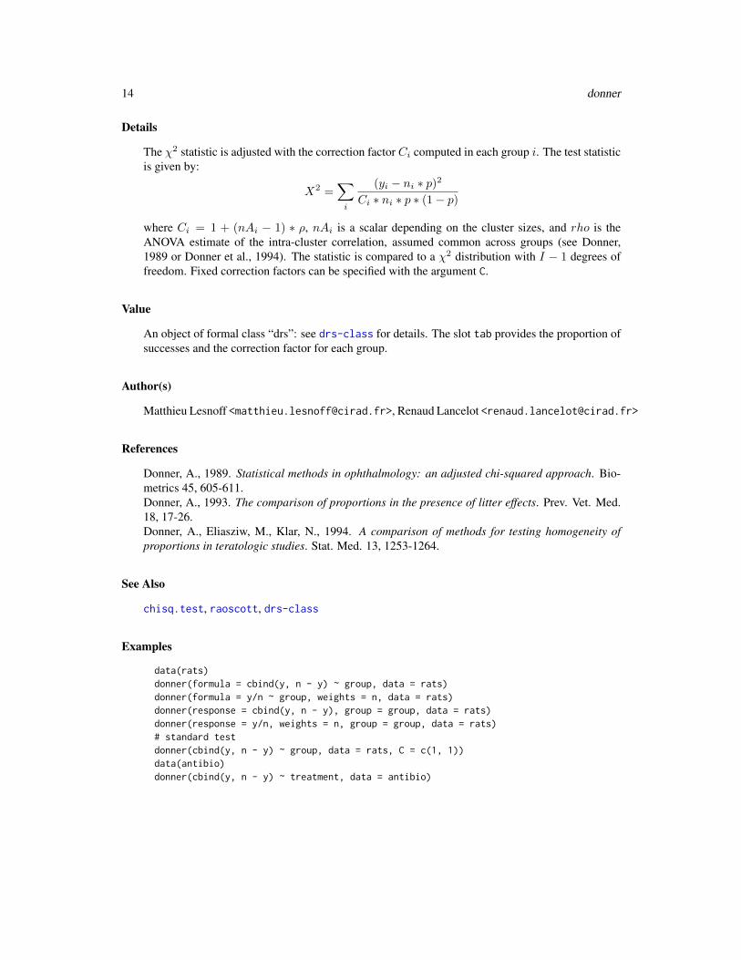
Details
The χ2 statistic is adjusted with the correction factor Ci computed in each group i. The test statisticis given by:
X2 =∑i
(yi − ni ∗ p)2
Ci ∗ ni ∗ p ∗ (1− p)
where Ci = 1 + (nAi − 1) ∗ ρ, nAi is a scalar depending on the cluster sizes, and rho is theANOVA estimate of the intra-cluster correlation, assumed common across groups (see Donner,1989 or Donner et al., 1994). The statistic is compared to a χ2 distribution with I − 1 degrees offreedom. Fixed correction factors can be specified with the argument C.
Value
An object of formal class “drs”: see drs-class for details. The slot tab provides the proportion ofsuccesses and the correction factor for each group.
Author(s)
Matthieu Lesnoff <[email protected]>, Renaud Lancelot <[email protected]>
References
Donner, A., 1989. Statistical methods in ophthalmology: an adjusted chi-squared approach. Bio-metrics 45, 605-611.Donner, A., 1993. The comparison of proportions in the presence of litter effects. Prev. Vet. Med.18, 17-26.Donner, A., Eliasziw, M., Klar, N., 1994. A comparison of methods for testing homogeneity ofproportions in teratologic studies. Stat. Med. 13, 1253-1264.
See Also
chisq.test, raoscott, drs-class
Examples
data(rats)donner(formula = cbind(y, n - y) ~ group, data = rats)donner(formula = y/n ~ group, weights = n, data = rats)donner(response = cbind(y, n - y), group = group, data = rats)donner(response = y/n, weights = n, group = group, data = rats)# standard testdonner(cbind(y, n - y) ~ group, data = rats, C = c(1, 1))data(antibio)donner(cbind(y, n - y) ~ treatment, data = antibio)
drs-class 15
drs-class Representation of Objects of Formal Class "drs"
Description
Representation of the output of functions donner and raoscott.
Objects from the Class
Objects can be created by calls of the form new("drs", ...) or, more commonly, via the donneror raoscott functions.
Slots
CALL The call of the function.
tab A data frame containing test information. The content of the data frame depends on the typeof the function which generated it.
rho The ANOVA estimate of the intra-cluster correlation (function donner).
X2 The adjusted χ2 statistic.
Methods
donner signature(object = "drs"): see donner.
raoscott signature(object = "drs"): see raoscott.
fitted-methods Methods for Function "fitted" in Package "aod"
Description
Extracts the fitted values from models.
Methods
ANY Generic function: see fitted.
glimML Extract the fitted values from models of formal class “glimML”, presently generated byfunctions betabin and negbin.
glimQL Extract the fitted values from models of formal class “glimQL”, presently generated byfunctions quasibin and quasibin.
16 glimML-class
glimML-class Representation of Models of Formal Class "glimML"
Description
Representation of models of formal class "glimML" fitted by maximum-likelihood method.
Objects from the Class
Objects can be created by calls of the form new("glimML", ...) or, more commonly, via thefunctions betabin or negbin.
Slots
CALL The call of the function.
link The link function used to transform the mean: “logit”, “cloglog” or “log”.
method The type of fitted model: “BB” for beta-binomial and “NB” for negative-binomial models.
formula The formula used to model the mean.
random The formula used to model the overdispersion parameter φ.
data Data set to which model was fitted. Different from the original data in case of missingvalue(s).
param The vector of the ML estimated parameters b and φ.
varparam The variance-covariance matrix of the ML estimated parameters b and φ.
fixed.param The vector of the ML estimated fixed-effect parameters b.
random.param The vector of the ML estimated random-effect (correlation) parameters φ.
logL The log-likelihood of the fitted model.
logL.max The log-likelihood of the maximal model (data).
dev The deviance of the model, i.e., - 2 * (logL - logL.max).
df.residual The residual degrees of freedom of the fitted model.
nbpar The number of estimated parameters, i.e., nbpar = total number of parameters - number offixed parameters. See argument fixpar in betabin or negbin.
iterations The number of iterations performed in optim.
code An integer (returned by optim) indicating why the optimization process terminated.
1 Relative gradient is close to 0, current iterate is probably solution.2 Successive iterates within tolerance, current iterate is probably solution.3 Last global step failed to locate a point lower than estimate. Either estimate is an approxi-
mate local minimum of the function or steptol is too small.4 Iteration limit exceeded.5 Maximum step size stepmax exceeded 5 consecutive times. Either the function is un-
bounded below, becomes asymptotic to a finite value from above in some direction orstepmax is too small.
glimQL-class 17
msg Message returned by optim.
singular.hessian Logical: true when fitting provided a singular hessian, indicating an overpara-materized model.
param.ini The initial values provided to the ML algorithm.
na.action A function defining the action taken when missing values are encountered.
glimQL-class Representation of Models of Formal Class "glimQL"
Description
Representation of models of formal class "glimQL" fitted by quasi-likelihood method.
Objects from the Class
Objects can be created by calls of the form new("glimQL", ...) or, more commonly, via thequasibin or quasipois functions.
Slots
CALL The call of the function.
fm A fitted model of class “glm”.
phi The overdispersion parameter.
Methods
show signature(object = "glimQL"): Main results of “glimQL” models.
iccbin Intra-Cluster Correlation for Binomial Data
Description
This function calculates point estimates of the intraclass correlation ρ from clustered binomialdata (n1, y1), (n2, y2), ..., (nK , yK) (with K the number of clusters), using a 1-way random ef-fect model. Three estimates, following methods referred to as “A”, “B” and “C” in Goldstein et al.(2002), can be obtained.
Usage
iccbin(n, y, data, method = c("A", "B", "C"), nAGQ = 1, M = 1000)
18 iccbin
Arguments
n Vector of the denominators of the proportions.
y Vector of the numerators of the proportions.
data A data frame containing the variables n and y.
method A character (“A”, “B” or “C”) defining the calculation method. See Details.
nAGQ Same as in function glmer of package lme4. Only for methods “A” and “B”.Default to 1.
M Number of Monte Carlo (MC) replicates used in method “B”. Default to 1000.
Details
Before computations, the clustered data are split into binary (0/1) observations yij (obs. j in clusteri). The calculation methods are described in Goldstein et al. (2002). Methods "A" and "B" assumea 1-way generalized linear mixed model, and method "C" a 1-way linear mixed model.For "A" and "B", function iccbin uses the logistic binomial-Gaussian model:
yij |pij ∼ Bernoulli(pij),
logit(pij) = b0 + ui,
where b0 is a constant and ui a cluster random effect with ui ∼ N(0, s2u). The ML estimate
of the variance component s2u is calculated with the function glmer of package lme4. The intra-
class correlation ρ = Corr[yij , yij′ ] is then calculated with a first-order model linearization aroundE[ui] = 0 in method “A”, and with Monte Carlo simulations in method “B”.For “C”, function iccbin provides the common ANOVA (moments) estimate of ρ. For details, seefor instance Donner (1986), Searle et al. (1992) or Ukoumunne (2002).
Value
An object of formal class “iccbin”, with 3 slots:
CALL The call of the function.
features A character vector summarizing the main features of the method used.
rho The point estimate of the intraclass correlation ρ.
Author(s)
Matthieu Lesnoff <[email protected]>, Renaud Lancelot <[email protected]>
References
Donner A., 1986, A review of inference procedures for the intraclass correlation coefficient in theone-way random effects model. International Statistical Review 54, 67-82.Searle, S.R., Casella, G., McCulloch, C.E., 1992. Variance components. Wiley, New York.Ukoumunne, O. C., 2002. A comparison of confidence interval methods for the intraclass correla-tion coefficient in cluster randomized trials. Statistics in Medicine 21, 3757-3774.Golstein, H., Browne, H., Rasbash, J., 2002. Partitioning variation in multilevel models. Under-standing Statistics 1(4), 223-231.
iccbin-class 19
See Also
iccbin-class, glmer
Examples
data(rats)tmp <- rats[rats$group == "TREAT", ]# A: glmm (model linearization)iccbin(n, y, data = tmp, method = "A")iccbin(n, y, data = tmp, method = "A", nAGQ = 10)# B: glmm (Monte Carlo)iccbin(n, y, data = tmp, method = "B")iccbin(n, y, data = tmp, method = "B", nAGQ = 10, M = 1500)# C: lmm (ANOVA moments)iccbin(n, y, data = tmp, method = "C")
## Not run:# Example of confidence interval calculation with nonparametric bootstraprequire(boot)foo <- function(X, ind) {
n <- X$n[ind]y <- X$y[ind]X <- data.frame(n = n, y = y)iccbin(n = n, y = y, data = X, method = "C")@rho[1]}
res <- boot(data = tmp[, c("n", "y")], statistic = foo, R = 500, sim = "ordinary", stype = "i")resboot.ci(res, conf = 0.95, type = "basic")
## End(Not run)
iccbin-class Representation of Objects of Formal Class "iccbin"
Description
Representation of the output of function iccbin.
Objects from the Class
Objects can be created by calls of the form new("iccbin", ...) or, more commonly, via thefunction iccbin.
20 invlink
Slots
CALL The call of the function.
features A character vector summarizing the main features of the method used.
rho A numeric scalar giving the intra-cluster correlation.
Methods
icc signature(object = "iccbin"): see iccbin.
invlink Transformation from the Link Scale to the Observation Scale
Description
The function transforms a variable from the link scale to the observation scale: probability or count.
Usage
invlink(x, type = c("cloglog", "log", "logit"))
Arguments
x A vector of real numbers.
type A character string. Legal values are “cloglog”, “log” and “logit”.
Value
anti− logit(x) = exp(x)/(1 + exp(x))anti− cloglog(x) = 1− exp(−exp(x))
See Also
link
Examples
x <- seq(-5, 5, length = 100)plot(x, invlink(x, type = "logit"),
type = "l", lwd = 2, ylab = "Probability")lines(x, invlink(x, type = "cloglog"), lty = 2, lwd = 2)grid(col = "black")legend(-5, 1, legend = c("alogit(x)", "acloglog(x)"),
lty = c(1, 2), bg = "white")
link 21
link Transformation from the Observation Scale to the Link Scale
Description
The function transforms a variable from the observation scale (probability or count) to the linkscale.
Usage
link(x, type = c("cloglog", "log", "logit"))
Arguments
x A vector of real numbers.
type A character string. Legal values are “cloglog”, “log” and “logit”.
Value
logit(x) = log(x/(1− x))cloglog(x) = log(−log(1− x))
See Also
invlink
Examples
x <- seq(.001, .999, length = 100)plot(x, link(x, type = "logit"),
type = "l", lwd = 2, ylab = "link(proba.)")lines(x, link(x, type = "cloglog"), lty = 2, lwd = 2)grid(col = "black")legend(0, 6, legend = c("logit(x)", "cloglog(x)"),
lty = c(1, 2), bg = "white")
lizards A Comparison of Site Preferences of Two Species of Lizard
Description
“These data describe the daytime habits of two species of lizards, grahami and opalinus. They werecollected by observing occupied sites or perches and recording the appropriate description, namelyspecies involved, time of the day, height and diameter of the perch and whether the site was sunnyor shaded. Time of the day is recorded as early, mid-day or late.” (McCullagh and Nelder, 1989,p.129).
22 logLik-methods
Usage
data(lizards)
Format
A data frame with 24 observations on the following 6 variables.
Site A factor with levels Sun and Shade.
Diameter A factor with levels D <= 2 and D > 2 (inches).
Height A factor with levels H < 5 and H >= 5 (feet).
Time A factor with levels Early, Mid-day and Late.
grahami A numeric vector giving the observed sample size for grahami lizards.
opalinus A numeric vector giving the observed sample size for opalinus lizards.
Details
The data were originally published in Fienberg (1970).
Source
McCullagh, P., Nelder, J.A., 1989. Generalized linear models. London, Chapman & Hall, 511 p.
References
Fienberg, S.E., 1970. The analysis of multidimensional contingency tables. Ecology 51: 419-433.
Examples
data(lizards)
logLik-methods Methods for Functions "logLik" in Package "aod"
Description
Extracts the maximized log-likelihood from fitted models of formal class “glimML”.
Usage
## S4 method for signature 'glimML'logLik(object, ...)
Arguments
object A fitted model of formal class “glimML” (functions betabin or negbin).
... Other arguments passed to methods.
mice 23
Value
A numeric scalar with 2 attributes: “df” (number of parameters in the model) and “nobs” (numberof observations = degrees of freedom of the residuals + number of parameters in the model).
Methods
ANY Generic function: see logLik.
glimML Extract the maximized log-likelihood from models of formal class “glimML”, fitted byfunctions betabin and negbin.
See Also
logLik in package stats.
mice Pregnant Female Mice Experiment
Description
Unpublished laboratory data on the proportion of affected foetuses in two groups (control and treat-ment) of 10 pregnant female mice (Kupper and Haseman, 1978, p. 75).
Usage
data(mice)
Format
A data frame with 20 observations on the following 3 variables.
group a factor with levels CTRL and TREAT
n a numeric vector: the total number of foetuses.
y a numeric vector: the number of affected foetuses.
References
Kupper, L.L., Haseman, J.K., 1978. The use of a correlated binomial model for the analysis of acertain toxicological experiments. Biometrics 34, 69-76.
24 negbin
negbin Negative-Binomial Model for Counts
Description
The function fits a negative-binomial log linear model accounting for overdispersion in counts y.
Usage
negbin(formula, random, data, phi.ini = NULL, warnings = FALSE,na.action = na.omit, fixpar = list(),hessian = TRUE, control = list(maxit = 2000), ...)
Arguments
formula A formula for the fixed effects. The left-hand side of the formula must be thecounts y i.e., positive integers (y >= 0). The right-hand side can involve anoffset term.
random A right-hand formula for the overdispersion parameter(s) φ.
data A data frame containing the response (y) and explanatory variable(s).
phi.ini Initial values for the overdispersion parameter(s) φ. Default to 0.1.
warnings Logical to control printing of warnings occurring during log-likelihood maxi-mization. Default to FALSE (no printing).
na.action A function name. Indicates which action should be taken in the case of missingvalue(s).
fixpar A list with 2 components (scalars or vectors) of the same size, indicating whichparameters are fixed (i.e., not optimized) in the global parameter vector (b, φ)and the corresponding fixed values.For example, fixpar = list(c(4, 5), c(0, 0)) means that 4th and 5thparameters of the model are set to 0.
hessian A logical. When set to FALSE, the hessian and the variances-covariances matri-ces of the parameters are not computed.
control A list to control the optimization parameters. See optim. By default, set themaximum number of iterations to 2000.
... Further arguments passed to optim.
Details
For a given count y, the model is:
y˜|˜λ ∼ Poisson(˜λ)
negbin 25
with λ following a Gamma distribution Gamma(r, ˜θ).If G denote the gamma function, then:
P (λ) = r−θ ∗ λθ−1 ∗exp(−λr )
G(θ)
E[λ] = θ ∗ r
V ar[λ] = θ ∗ r2
The marginal negative-binomial distribution is:
P (y) = G(y + θ) ∗(
1
1 + r
)θ∗
( r1+r )y
y! ∗G(θ)
The function uses the parameterization µ = θ ∗ r = exp(Xb) = exp(η) and φ = 1/θ, where X is adesign-matrix, b is a vector of fixed effects, η = Xb is the linear predictor and φ the overdispersionparameter.The marginal mean and variance are:
E[y] = µ
V ar[y] = µ+ φ ∗ µ2
The parameters b and φ are estimated by maximizing the log-likelihood of the marginal model(using the function optim()). Several explanatory variables are allowed in b. Only one is allowedin φ.An offset can be specified in the formula argument to model rates y/T . The offset and the marginalmean are log(T ) and µ = exp(log(T ) + η), respectively.
Value
An object of formal class “glimML”: see glimML-class for details.
Author(s)
Matthieu Lesnoff <[email protected]>, Renaud Lancelot <[email protected]>
References
Lawless, J.F., 1987. Negative binomial and mixed Poisson regression. The Canadian Journal ofStatistics, 15(3): 209-225.
See Also
glimML-class, glm and optim,glm.nb in the recommended package MASS,gnlr in package gnlm available at www.luc.ac.be/~jlindsey/rcode.html.
26 orob1
Examples
# without offsetdata(salmonella)negbin(y ~ log(dose + 10) + dose, ~ 1, salmonella)library(MASS) # function glm.nb in MASSfm.nb <- glm.nb(y ~ log(dose + 10) + dose,
link = log, data = salmonella)coef(fm.nb)1 / fm.nb$theta # theta = 1 / phic(logLik(fm.nb), AIC(fm.nb))# with offsetdata(dja)negbin(y ~ group + offset(log(trisk)), ~ group, dja)# phi fixed to zero in group TREATnegbin(y ~ group + offset(log(trisk)), ~ group, dja,
fixpar = list(4, 0))# glim without overdispersionsummary(glm(y ~ group + offset(log(trisk)),
family = poisson, data = dja))# phi fixed to zero in both groupsnegbin(y ~ group + offset(log(trisk)), ~ group, dja,
fixpar = list(c(3, 4), c(0, 0)))
orob1 Germination Data
Description
[Data describing the germination] “for seed Orobanche cernua cultivated in three dilutions of abean root extract. The mean proportions of the three sets are 0.142, 0.872 and 0.842, and the overallmean is 0.614.” (Crowder, 1978, Table 1).
Usage
data(orob1)
Format
A data frame with 16 observations on the following 3 variables.
dilution a factor with 3 levels: 1/1, 1/25 and 1/625.
n a numeric vector: the number of seeds exposed to germination.
y a numeric vector: the number of seeds which actually germinated.
References
Crowder, M.J., 1978. Beta-binomial anova for proportions. Appl. Statist. 27, 34-37.
orob2 27
orob2 Germination Data
Description
“A 2 x 2 factorial experiment comparing 2 types of seed and 2 root extracts. There are 5 or 6replicates in each of the 4 treatment groups, and each replicate comprises a number of seeds varyingbetween 4 and 81. The response variable is the proportion of seeds germinating in each replicate.”(Crowder, 1978, Table 3).
Usage
data(orob2)
Format
A data frame with 21 observations on the following 4 variables.
seed a factor with 2 levels: O73 and O75.
root a factor with 2 levels BEAN and CUCUMBER.
n a numeric vector: the number of seeds exposed to germination.
y a numeric vector: the number of seeds which actually germinated.
References
Crowder, M.J., 1978. Beta-binomial anova for proportions. Appl. Statist. 27, 34-37.
predict-methods Methods for Function "predict" in Package "aod"
Description
“predict” methods for fitted models generated by functions in package aod.
Usage
## S4 method for signature 'glimML'predict(object, newdata = NULL,
type = c("response", "link"), se.fit = FALSE, ...)## S4 method for signature 'glimQL'
predict(object, newdata = NULL,type = c("response", "link"), se.fit = FALSE, ...)
28 quasibin
Arguments
object A fitted model of formal class “glimML” (functions betabin or negbin) or“glimQL” (functions quasibin or quasipois).
newdata A data.frame providing all the explanatory variables necessary for predictions.
type A character string indicating the scale on which predictions are made: either“response” for predictions on the observation scale, or “link” for predictions onthe scale of the link.
se.fit A logical scalar indicating whether pointwise standard errors should be com-puted for the predictions.
... Other arguments passed to methods.
Methods
glimML Compute predictions for models of formal class “glimML”, presently generated by func-tions betabin and negbin. See the examples for these functions.
glimQL Compute predictions for models of formal class “glimQL”, presently generated by thefunctions quasibin and quasibin. See the examples for these functions.
See Also
predict.glm
quasibin Quasi-Likelihood Model for Proportions
Description
The function fits the generalized linear model “II” proposed by Williams (1982) accounting foroverdispersion in clustered binomial data (n, y).
Usage
quasibin(formula, data, link = c("logit", "cloglog"), phi = NULL, tol = 0.001)
Arguments
formula A formula for the fixed effects. The left-hand side of the formula must be of theform cbind(y, n - y) where the modelled probability is y/n.
link The link function for the mean p: “logit” or “cloglog”.
data A data frame containing the response (n and y) and explanatory variable(s).
phi When phi is NULL (the default), the overdispersion parameter φ is estimatedfrom the data. Otherwise, its value is considered as fixed.
tol A positive scalar (default to 0.001). The algorithm stops at iteration r + 1 whenthe condition χ2[r + 1]− χ2[r] <= tol is met by the χ2 statistics .
quasibin 29
Details
For a given cluster (n, y), the model is:
y˜|˜λ ∼ Binomial(n, ˜λ)
with λ a random variable of mean E[λ] = p and variance V ar[λ] = φ ∗ p ∗ (1− p).The marginal mean and variance are:
E[y] = p
V ar[y] = p ∗ (1− p) ∗ [1 + (n− 1) ∗ φ]
The overdispersion parameter φ corresponds to the intra-cluster correlation coefficient, which ishere restricted to be positive.The function uses the function glm and the parameterization: p = h(Xb) = h(η), where h is theinverse of a given link function, X is a design-matrix, b is a vector of fixed effects and η = Xb isthe linear predictor.The estimate of b maximizes the quasi log-likelihood of the marginal model. The parameter φ isestimated with the moment method or can be set to a constant (a regular glim is fitted when φ is setto zero). The literature recommends to estimate φ from the saturated model. Several explanatoryvariables are allowed in b. None is allowed in φ.
Value
An object of formal class “glimQL”: see glimQL-class for details.
Author(s)
Matthieu Lesnoff <[email protected]>, Renaud Lancelot <[email protected]>
References
Moore, D.F., 1987, Modelling the extraneous variance in the presence of extra-binomial variation.Appl. Statist. 36, 8-14.Williams, D.A., 1982, Extra-binomial variation in logistic linear models. Appl. Statist. 31, 144-148.
See Also
glm, geese in the contributed package geepack, glm.binomial.disp in the contributed packagedispmod.
Examples
data(orob2)fm1 <- glm(cbind(y, n - y) ~ seed * root,
family = binomial, data = orob2)fm2 <- quasibin(cbind(y, n - y) ~ seed * root,
data = orob2, phi = 0)fm3 <- quasibin(cbind(y, n - y) ~ seed * root,
data = orob2)rbind(fm1 = coef(fm1), fm2 = coef(fm2), fm3 = coef(fm3))
30 quasipois
# show the modelfm3# dispersion parameter and goodness-of-fit statisticc(phi = fm3@phi,
X2 = sum(residuals(fm3, type = "pearson")^2))# model predictionspredfm1 <- predict(fm1, type = "response", se = TRUE)predfm3 <- predict(fm3, type = "response", se = TRUE)New <- expand.grid(seed = levels(orob2$seed),
root = levels(orob2$root))predict(fm3, New, se = TRUE, type = "response")data.frame(orob2, p1 = predfm1$fit,
se.p1 = predfm1$se.fit,p3 = predfm3$fit,se.p3 = predfm3$se.fit)
fm4 <- quasibin(cbind(y, n - y) ~ seed + root,data = orob2, phi = fm3@phi)
# Pearson's chi-squared goodness-of-fit statistic# compare with fm3's X2sum(residuals(fm4, type = "pearson")^2)
quasipois Quasi-Likelihood Model for Counts
Description
The function fits the log linear model (“Procedure II”) proposed by Breslow (1984) accounting foroverdispersion in counts y.
Usage
quasipois(formula, data, phi = NULL, tol = 0.001)
Arguments
formula A formula for the fixed effects. The left-hand side of the formula must be thecounts y i.e., positive integers (y >= 0). The right-hand side can involve anoffset term.
data A data frame containing the response (y) and explanatory variable(s).
phi When phi is NULL (the default), the overdispersion parameter φ is estimatedfrom the data. Otherwise, its value is considered as fixed.
tol A positive scalar (default to 0.001). The algorithm stops at iteration r + 1 whenthe condition χ2[r + 1]− χ2[r] <= tol is met by the χ2 statistics .
quasipois 31
Details
For a given count y, the model is:
y˜|˜λ ∼ Poisson(˜λ)
with λ a random variable of mean E[λ] = µ and variance V ar[λ] = φ ∗ µ2.The marginal mean and variance are:
E[y] = µ
V ar[y] = µ+ φ ∗ µ2
The function uses the function glm and the parameterization: µ = exp(Xb) = exp(η), where X isa design-matrix, b is a vector of fixed effects and η = Xb is the linear predictor.The estimate of b maximizes the quasi log-likelihood of the marginal model. The parameter φ isestimated with the moment method or can be set to a constant (a regular glim is fitted when φ isset to 0). The literature recommends to estimate φ with the saturated model. Several explanatoryvariables are allowed in b. None is allowed in φ.An offset can be specified in the argument formula to model rates y/T (see examples). The offsetand the marginal mean are log(T ) and µ = exp(log(T ) + η), respectively.
Value
An object of formal class “glimQL”: see glimQL-class for details.
Author(s)
Matthieu Lesnoff <[email protected]>, Renaud Lancelot <[email protected]>
References
Breslow, N.E., 1984. Extra-Poisson variation in log-linear models. Appl. Statist. 33, 38-44.Moore, D.F., Tsiatis, A., 1991. Robust estimation of the variance in moment methods for extra-binomial and extra-poisson variation. Biometrics 47, 383-401.
See Also
glm, negative.binomial in the recommended package MASS, geese in the contributed packagegeepack, glm.poisson.disp in the contributed package dispmod.
Examples
# without offsetdata(salmonella)quasipois(y ~ log(dose + 10) + dose,
data = salmonella)quasipois(y ~ log(dose + 10) + dose,
data = salmonella, phi = 0.07180449)summary(glm(y ~ log(dose + 10) + dose,
family = poisson, data = salmonella))quasipois(y ~ log(dose + 10) + dose,
data = salmonella, phi = 0)
32 rabbits
# with offsetdata(cohorts)i <- cohorts$age ; levels(i) <- 1:7j <- cohorts$period ; levels(j) <- 1:7i <- as.numeric(i); j <- as.numeric(j)cohorts$cohort <- j + max(i) - icohorts$cohort <- as.factor(1850 + 5 * cohorts$cohort)fm1 <- quasipois(y ~ age + period + cohort + offset(log(n)),
data = cohorts)fm1quasipois(y ~ age + cohort + offset(log(n)),
data = cohorts, phi = fm1@phi)
rabbits Rabbits Foetuses Survival Experiment
Description
Experimental data for analyzing the effect of an increasing dose of a compound on the proportion oflive foetuses affected. Four treatment-groups were considered: control “C”, low dose “L”, mediumdose “M” and high dose “H”. The animal species used in the experiment was banded Dutch rabbit(Paul, 1982, Table 1).
Usage
data(rabbits)
Format
A data frame with 84 observations on the following 3 variables.
group a factor with levels C, H, L and M
n a numeric vector: the total number of foetuses.
y a numeric vector: the number of affected foetuses.
References
Paul, S.R., 1982. Analysis of proportions of affected foetuses in teratological experiments. Biomet-rics 38, 361-370.
raoscott 33
raoscott Test of Proportion Homogeneity using Rao and Scott’s Adjustment
Description
Tests the homogeneity of proportions between I groups (H0: p1 = p2 = ... = pI ) from clusteredbinomial data (n, y) using the adjusted χ2 statistic proposed by Rao and Scott (1993).
Usage
raoscott(formula = NULL, response = NULL, weights = NULL,group = NULL, data, pooled = FALSE, deff = NULL)
Arguments
formula An optional formula where the left-hand side is either a matrix of the formcbind(y, n-y), where the modelled probability is y/n, or a vector of pro-portions to be modelled (y/n). In both cases, the right-hand side must specify asingle grouping variable. When the left-hand side of the formula is a vector ofproportions, the argument weight must be used to indicate the denominators ofthe proportions.
response An optional argument: either a matrix of the form cbind(y, n-y), where themodelled probability is y/n, or a vector of proportions to be modelled (y/n).
weights An optional argument used when the left-hand side of formula or response isa vector of proportions: weight is the denominator of the proportions.
group An optional argument only used when response is used. In this case, this argu-ment is a factor indicating a grouping variable.
data A data frame containing the response (n and y) and the grouping variable.
pooled Logical indicating if a pooled design effect is estimated over the I groups.
deff A numerical vector of I design effects.
Details
The method is based on the concepts of design effect and effective sample size.
The design effect in each group i is estimated by deffi = vratioi/vbini, where vratioi is thevariance of the ratio estimate of the probability in group i (Cochran, 1999, p. 32 and p. 66) andvbini is the standard binomial variance. A pooled design effect (i.e., over the I groups) is estimatedif argument pooled = TRUE (see Rao and Scott, 1993, Eq. 6). Fixed design effects can be specifiedwith the argument deff.The deffi are used to compute the effective sample sizes nadji = ni/deffi, the effective num-bers of successes yadji = yi/deffi in each group i, and the overall effective proportion padj =∑i yadji/
∑i deffi. The test statistic is obtained by substituting these quantities in the usual χ2
statistic, yielding:
X2 =∑i
(yadji − nadji ∗ padj)2
nadji ∗ padj ∗ (1− padj)
34 rats
which is compared to a χ2 distribution with I − 1 degrees of freedom.
Value
An object of formal class “drs”: see drs-class for details. The slot tab provides the proportion ofsuccesses, the variances of the proportion and the design effect for each group.
Author(s)
Matthieu Lesnoff <[email protected]>, Renaud Lancelot <[email protected]>
References
Cochran, W.G., 1999, 2nd ed. Sampling techniques. John Wiley & Sons, New York.Rao, J.N.K., Scott, A.J., 1992. A simple method for the analysis of clustered binary data. Biometrics48, 577-585.
See Also
chisq.test, donner, iccbin, drs-class
Examples
data(rats)# deff by groupraoscott(cbind(y, n - y) ~ group, data = rats)raoscott(y/n ~ group, weights = n, data = rats)raoscott(response = cbind(y, n - y), group = group, data = rats)raoscott(response = y/n, weights = n, group = group, data = rats)# pooled deffraoscott(cbind(y, n - y) ~ group, data = rats, pooled = TRUE)# standard testraoscott(cbind(y, n - y) ~ group, data = rats, deff = c(1, 1))data(antibio)raoscott(cbind(y, n - y) ~ treatment, data = antibio)
rats Rats Diet Experiment
Description
“Weil (1970) in Table 1 gives the results from an experiment comprising two treatments. One groupof 16 pregnant female rats was fed a control diet during pregnancy and lactation, the diet of a secondgroup of 16 pregnant females was treated with a chemical. For each litter the number n of pupsalive at 4 days and the number x of pups that survived the 21 day lactation period were recorded.”(Williams, 1975, p. 951).
residuals-methods 35
Usage
data(rats)
Format
A data frame with 32 observations on the following 3 variables.
group A factor with levels CTRL and TREAT
n A numeric vector: the number of pups alive at 4 days.
y A numeric vector: the number of pups that survived the 21 day lactation.
Source
Williams, D.A., 1975. The analysis of binary responses from toxicological experiments involvingreproduction and teratogenicity. Biometrics 31, 949-952.
References
Weil, C.S., 1970. Selection of the valid number of sampling units and a consideration of theircombination in toxicological studies involving reproduction, teratogenesis or carcinogenesis. Fd.Cosmet. Toxicol. 8, 177-182.
residuals-methods Residuals for Maximum-Likelihood and Quasi-Likelihood Models
Description
Residuals of models fitted with functions betabin and negbin (formal class “glimML”), or quasibinand quasipois (formal class “glimQL”).
Usage
## S4 method for signature 'glimML'residuals(object, type = c("pearson", "response"), ...)## S4 method for signature 'glimQL'
residuals(object, type = c("pearson", "response"), ...)
Arguments
object Fitted model of formal class “glimML” or “glimQL”.
type Character string for the type of residual: “pearson” (default) or “response”.
... Further arguments to be passed to the function, such as na.action.
36 salmonella
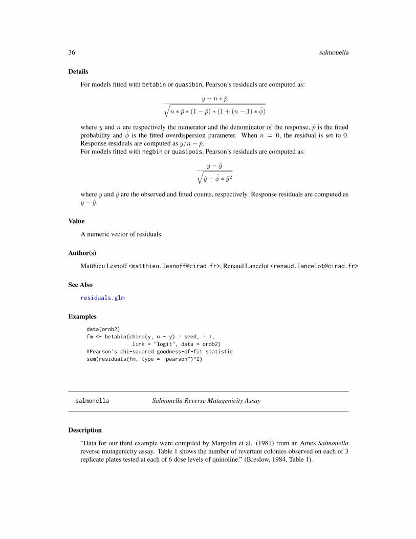
Details
For models fitted with betabin or quasibin, Pearson’s residuals are computed as:
y − n ∗ p√n ∗ p ∗ (1− p) ∗ (1 + (n− 1) ∗ φ)
where y and n are respectively the numerator and the denominator of the response, p is the fittedprobability and φ is the fitted overdispersion parameter. When n = 0, the residual is set to 0.Response residuals are computed as y/n− p.For models fitted with negbin or quasipois, Pearson’s residuals are computed as:
y − y√y + φ ∗ y2
where y and y are the observed and fitted counts, respectively. Response residuals are computed asy − y.
Value
A numeric vector of residuals.
Author(s)
Matthieu Lesnoff <[email protected]>, Renaud Lancelot <[email protected]>
See Also
residuals.glm
Examples
data(orob2)fm <- betabin(cbind(y, n - y) ~ seed, ~ 1,
link = "logit", data = orob2)#Pearson's chi-squared goodness-of-fit statisticsum(residuals(fm, type = "pearson")^2)
salmonella Salmonella Reverse Mutagenicity Assay
Description
“Data for our third example were compiled by Margolin et al. (1981) from an Ames Salmonellareverse mutagenicity assay. Table 1 shows the number of revertant colonies observed on each of 3replicate plates tested at each of 6 dose levels of quinoline.” (Breslow, 1984, Table 1).
splitbin 37
Usage
data(salmonella)
Format
A data frame with 18 observations on the following 2 variables.
dose a numeric vector: the dose level of quinoline (microgram per plate).
y a numeric vector: the number of revertant colonies of TA98 Salmonella.
Source
Breslow, N.E., 1984. Extra-Poisson variation in log-linear models. Applied Statistics 33(1), 38-44.
References
Margolin, B.H., Kaplan, N., Zeiger, E., 1981. Statistical analysis of the Ames Salmonella / micro-some test. Proc. Natl Acad. Sci. USA 76, 3779-3783.
splitbin Split Grouped Data Into Individual Data
Description
The function splits grouped data and optional covariates into individual data. Two types of groupeddata are managed by splitbin:
• Grouped data with weights;
• Grouped data of form cbind(success, failure).
When weights, successes or failures involve non-integer numbers, these numbers are rounded beforesplitting.
Usage
splitbin(formula, data, id = "idbin")
Arguments
formula A formula. The left-hand side represents grouped data. The right-hand sidedefines the covariates. See examples for syntax.
data A data frame where all the variables described in formula are found.
id An optional character string naming the identifier (= grouping factor). Defaultto “idbin”.
38 summary,aic-method
Value
A data frame built according to the formula and function used in the call.
Examples
# Grouped data with weightsmydata <- data.frame(
success = c(0, 1, 0, 1),f1 = c("A", "A", "B", "B"),f2 = c("C", "D", "C", "D"),n = c(4, 2, 1, 3))
mydatasplitbin(formula = n ~ f1, data = mydata)$tabsplitbin(formula = n ~ f1 + f2 + success , data = mydata)$tab
# Grouped data of form "cbind(success, failure)"mydata <- data.frame(
success = c(4, 1),failure = c(1, 2),f1 = c("A", "B"),f2 = c("C", "D"))
mydata$n <- mydata$success + mydata$failuremydatasplitbin(formula = cbind(success, failure) ~ 1, data = mydata)$tabsplitbin(formula = cbind(success, failure) ~ f1 + f2, data = mydata)$tabsplitbin(formula = cbind(success, n - success) ~ f1 + f2, data = mydata)$tabsplitbin(formula = cbind(success, n - 0.5 * failure - success) ~ f1 + f2,
data = mydata)$tab
summary,aic-method Akaike Information Statistics
Description
Computes Akaike difference and Akaike weights from an object of formal class “aic”.
Usage
## S4 method for signature 'aic'summary(object, which = c("AIC", "AICc"))
Arguments
object An object of formal class “aic”.
which A character string indicating which information criterion is selected to computeAkaike difference and Akaike weights: either “AIC” or “AICc”.
summary.glimML-class 39
Methods
summary The models are ordered according to AIC or AICc and 3 statistics are computed:- the Akaike difference ∆: the change in AIC (or AICc) between successive (ordered) models,- the Akaike weight W : when r models are compared, W = e−0.5∗∆/
∑r e
− 12∗∆,
- the cumulative Akaike weight cum.W : the Akaike weights sum to 1 for the r models whichare compared.
References
Burnham, K.P., Anderson, D.R., 2002. Model selection and multimodel inference: a practicalinformation-theoretic approach. New-York, Springer-Verlag, 496 p.Hurvich, C.M., Tsai, C.-L., 1995. Model selection for extended quasi-likelihood models in smallsamples. Biometrics, 51 (3): 1077-1084.
See Also
Examples in betabin and AIC in package stats.
summary.glimML-class Summary of Objects of Class "summary.glimML"
Description
Summary of a model of formal class “glimML” fitted by betabin or negbin.
Objects from the Class
Objects can be created by calls of the form new("summary.glimML", ...) or, more commonly,via the summary or show method for objects of formal class “glimML”.
Slots
object An object of formal class “glimML”.
Coef A data frame containing the estimates, standard error, z and P values for the fixed-effectcoefficients which were estimated by the fitting function.
FixedCoef A data frame containing the values of the fixed-effect coefficients which were set to afixed value.
Phi A data frame containing the estimates, standard error, z and P values for the overdispersioncoefficients which were estimated by the fitting function. Because the overdispersion coeffi-cients are > 0, P values correspond to unilateral tests.
FixedPhi A data frame containing the values of the overdispersion coefficients which were set toa fixed value.
40 varbin
Methods
show signature(object = "summary.glimML")
show signature(object = "glimML")
summary signature(object = "glimML")
Examples
data(orob2)fm1 <- betabin(cbind(y, n - y) ~ seed, ~ 1, data = orob2)# show objects of class "glimML"fm1# summary for objects of class "glimML"res <- summary(fm1)res@Coef# show objects of class "summary.glimML"res
varbin Mean, Variance and Confidence Interval of a Proportion
Description
This function computes the mean and variance of a proportion from clustered binomial data (n, y),using various methods. Confidence intervals are computed using a normal approximation, whichmight be inappropriate when the proportion is close to 0 or 1.
Usage
varbin(n, y, data, alpha = 0.05, R = 5000)
Arguments
n The denominator of the proportion.
y The numerator of the proportion.
data A data frame containing the data.
alpha The significance level for the confidence intervals. Default to 0.05, providing95% CI’s.
R The number of bootstrap replicates to compute the bootstrap mean and variance.
varbin 41
Details
Five methods are used for the estimations. Let us consider N clusters of sizes n1, . . . , nN withobserved responses (counts) y1, . . . , yN . We note pi = yi/ni the observed proportions (i =1, . . . , N). An underlying assumption is that the theoretical proportion is homogeneous acrossthe clusters.
Binomial method: the proportion and its variance are estimated as p =
∑iyi∑
ini
and p∗(1−p)∑ini−1
,
respectively.
Ratio method: the one-stage cluster sampling formula is used to estimate the variance of the ratioestimate (see Cochran, 1999, p. 32 and p. 66). The proportion is estimated as above (p).
Arithmetic method: the proportion is estimated as pA = 1N
∑iyini
, with estimated variance∑i(pi−pA)2
N∗(N−1) .
Jackknife method: the proportion pJ is the arithmetic mean of the pseudovalues pvi, with esti-
mated variance∑
i(pvi−pJ )2
N∗(N−1) (Gladen, 1977, Paul, 1982).
Bootstrap method: R samples of size N are drawn with equal probability from the initial sample(p1, . . . , pN ) (Efron and Tibshirani, 1993). The bootstrap estimate pB and its estimated varianceare the arithmetic mean and the empirical variance (computed with denominator R − 1) of the Rbinomial estimates, respectively.
Value
An object of formal class “varbin”, with 5 slots:
CALL The call of the function.tab A 4-column data frame giving for each estimation method the mean, variance,
upper and lower limits of the (1− α) confidence interval.boot A numeric vector containing the R bootstrap replicates of the proportion. Might
be used to compute other kinds of CI’s for the proportion.alpha The significance level used to compute the (1− α) confidence intervals.features A numeric vector with 3 components summarizing the main features of the data:
N = number of clusters, n = number of subjects, y = number of cases.
The “show” method displays the slot tab described above, substituting the standard error to thevariance.
Author(s)
Matthieu Lesnoff <[email protected]>, Renaud Lancelot <[email protected]>
References
Cochran, W.G., 1999, 3th ed. Sampling techniques. Wiley, New York.Efron, B., Tibshirani, R., 1993. An introduction to the bootstrap. Chapman and Hall, London.Gladen, B., 1977. The use of the jackknife to estimate proportions from toxicological data in thepresence of litter effects. JASA 74(366), 278-283.Paul, S.R., 1982. Analysis of proportions of affected foetuses in teratological experiments. Biomet-rics 38, 361-370.
42 varbin-class
See Also
varbin-class, boot
Examples
data(rabbits)varbin(n, y, rabbits[rabbits$group == "M", ])by(rabbits,
list(group = rabbits$group),function(x) varbin(n = n, y = y, data = x, R = 1000))
varbin-class Representation of Objects of Formal Class "varbin"
Description
Representation of the output of function varbin used to estimate proportions and their varianceunder various distribution assumptions.
Objects from the Class
Objects can be created by calls of the form new("varbin", ...) or, more commonly, via thefunction varbin.
Slots
CALL The call of the function.
tab A data frame containing the estimates, their variance and the confidence limits.
pboot A numeric vector containing the bootstrap replicates.
alpha The α level to compute confidence intervals.
features A named numeric vector summarizing the design.
Methods
varbin signature(object = "varbin"): see varbin.
vcov-methods 43
vcov-methods Methods for Function "vcov" in Package "aod"
Description
Extract the approximate var-cov matrix of estimated coefficients from fitted models.
Methods
ANY Generic function: see vcov.
glimML Extract the var-cov matrix of estimated coefficients for fitted models of formal class“glimML”.
glimQL Extract the var-cov matrix of estimated coefficients for fitted models of formal class“glimQL”.
geese Extract the var-cov matrix of estimated coefficients for fitted models of class “geese” (con-tributed package geepack).
geeglm Extract the var-cov matrix of estimated coefficients for fitted objects of class “geeglm”(contributed package geepack).
wald.test Wald Test for Model Coefficients
Description
Computes a Wald χ2 test for 1 or more coefficients, given their variance-covariance matrix.
Usage
wald.test(Sigma, b, Terms = NULL, L = NULL, H0 = NULL,df = NULL, verbose = FALSE)
## S3 method for class 'wald.test'print(x, digits = 2, ...)
Arguments
Sigma A var-cov matrix, usually extracted from one of the fitting functions (e.g., lm,glm, ...).
b A vector of coefficients with var-cov matrix Sigma. These coefficients are usu-ally extracted from one of the fitting functions available in R (e.g., lm, glm,...).
Terms An optional integer vector specifying which coefficients should be jointly tested,using a Wald χ2 or F test. Its elements correspond to the columns or rows ofthe var-cov matrix given in Sigma. Default is NULL.
44 wald.test
L An optional matrix conformable to b, such as its product with b i.e., L %*% bgives the linear combinations of the coefficients to be tested. Default is NULL.
H0 A numeric vector giving the null hypothesis for the test. It must be as long asTerms or must have the same number of columns as L. Default to 0 for all thecoefficients to be tested.
df A numeric vector giving the degrees of freedom to be used in an F test, i.e.the degrees of freedom of the residuals of the model from which b and Sigmawere fitted. Default to NULL, for no F test. See the section Details for moreinformation.
verbose A logical scalar controlling the amount of output information. The default isFALSE, providing minimum output.
x Object of class “wald.test”
digits Number of decimal places for displaying test results. Default to 2.
... Additional arguments to print.
Details
The key assumption is that the coefficients asymptotically follow a (multivariate) normal distribu-tion with mean = model coefficients and variance = their var-cov matrix.One (and only one) of Terms or L must be given. When L is given, it must have the same numberof columns as the length of b, and the same number of rows as the number of linear combinationsof coefficients. When df is given, the χ2 Wald statistic is divided by m = the number of linear com-binations of coefficients to be tested (i.e., length(Terms) or nrow(L)). Under the null hypothesisH0, this new statistic follows an F (m, df) distribution.
Value
An object of class wald.test, printed with print.wald.test.
References
Diggle, P.J., Liang, K.-Y., Zeger, S.L., 1994. Analysis of longitudinal data. Oxford, ClarendonPress, 253 p.Draper, N.R., Smith, H., 1998. Applied Regression Analysis. New York, John Wiley & Sons, Inc.,706 p.
See Also
vcov
Examples
data(orob2)fm <- quasibin(cbind(y, n - y) ~ seed * root, data = orob2)# Wald test for the effect of rootwald.test(b = coef(fm), Sigma = vcov(fm), Terms = 3:4)
Index
∗Topic classesaic-class, 2drs-class, 15glimML-class, 16glimQL-class, 17iccbin-class, 19summary.glimML-class, 39varbin-class, 42
∗Topic datagensplitbin, 37
∗Topic datasetsantibio, 5cohorts, 11dja, 12lizards, 21mice, 23orob1, 26orob2, 27rabbits, 32rats, 34salmonella, 36
∗Topic htestdonner, 13iccbin, 17raoscott, 33varbin, 40wald.test, 43
∗Topic mathinvlink, 20link, 21
∗Topic methodsAIC-methods, 3coef-methods, 10deviance-methods, 11df.residual-methods, 12fitted-methods, 15logLik-methods, 22predict-methods, 27summary,aic-method, 38
vcov-methods, 43∗Topic package
aod-pkg, 6∗Topic regression
anova-methods, 4betabin, 7negbin, 24quasibin, 28quasipois, 30residuals-methods, 35
AIC, 3–5, 39AIC,glimML-method (AIC-methods), 3aic-class, 2AIC-methods, 3anova,glimML-method (anova-methods), 4anova-methods, 4anova.glimML-class (anova-methods), 4anova.glm, 5antibio, 5aod (aod-pkg), 6aod-pkg, 6
betabin, 4, 7, 16, 28, 39boot, 42
chisq.test, 14, 34coef, 10coef,glimML-method (coef-methods), 10coef,glimQL-method (coef-methods), 10coef-methods, 10cohorts, 11
deviance, 11deviance,glimML-method
(deviance-methods), 11deviance-methods, 11df.residual, 12df.residual,glimML-method
(df.residual-methods), 12
45
46 INDEX
df.residual,glimQL-method(df.residual-methods), 12
df.residual-methods, 12dja, 12donner, 13, 15, 34drs-class, 15
fitted, 15fitted,glimML-method (fitted-methods),
15fitted,glimQL-method (fitted-methods),
15fitted-methods, 15
geeglm-class (vcov-methods), 43geese, 29, 31geese-class (vcov-methods), 43glimML-class, 16glimQL-class, 17glm, 9, 25, 29, 31glm.binomial.disp, 29glm.nb, 25glm.poisson.disp, 31glmer, 19
iccbin, 17, 20, 34iccbin-class, 19invlink, 20, 21
link, 20, 21lizards, 21logLik, 23logLik,glimML-method (logLik-methods),
22logLik-methods, 22
mice, 23
negative.binomial, 31negbin, 16, 24, 28
optim, 8, 9, 24, 25orob1, 26orob2, 27
predict,glimML-method(predict-methods), 27
predict,glimQL-method(predict-methods), 27
predict-methods, 27
predict.glm, 28print.wald.test (wald.test), 43
quasibin, 28, 28quasipois, 30
rabbits, 32raoscott, 14, 15, 33rats, 34residuals,glimML-method
(residuals-methods), 35residuals,glimQL-method
(residuals-methods), 35residuals-methods, 35residuals.glm, 36
salmonella, 36show,aic-method (summary,aic-method), 38show,anova.glimML-method
(anova-methods), 4show,donner-class (donner), 13show,drs-method (drs-class), 15show,glimML-class
(summary.glimML-class), 39show,glimML-method (glimML-class), 16show,glimQL-method (glimQL-class), 17show,iccbin-method (iccbin), 17show,raoscott-class (raoscott), 33show,summary.glimML-method
(summary.glimML-class), 39show,varbin-class (varbin), 40show,varbin-method (varbin-class), 42splitbin, 37summary,aic-method, 38summary,glimML-method
(summary.glimML-class), 39summary.glimML-class, 39
varbin, 40, 42varbin-class, 42vcov, 43, 44vcov,geeglm-method (vcov-methods), 43vcov,geese-method (vcov-methods), 43vcov,glimML-method (vcov-methods), 43vcov,glimQL-method (vcov-methods), 43vcov-methods, 43
wald.test, 43