Pacific Fog Climatologies

Cindy Combs

CIRA/Colorado State University

While global climatologies are required for climate models and other interests, they are usually too large and at resolutions too low to be useful for an average forecaster. National Weather Service (NWS) offices are more concern with local features and phenomena that occur in their area. These events can be small in nature and change during a short time period.

CIRA has a long history of producing high resolution, satellite cloud climatologies from GOES images for given regions. They have been used to find cloud patterns that bring new insights to local conditions.

By working with forecasters, climatologies can be tailored to meet their needs. This talk will provide an introduction to Regional Cloud Climatologies and then will concentrate on the Pacific Coast.

INTRODUCTION

What are Regional Cloud Climatologies?

They are climatologies focused on the cloud patterns of a particular location and what influences them.

Each region has its own terrain features, which can include rivers, oceans, mountains, agricultural areas, etc.

They are also subjected to common, overall weather patterns such as sea breezes or synoptic systems.

All of these features can interact with each other to produce conditions unique to that region. Cloud patterns are influenced by these many factors, and can be used to determine current conditions or forecast future ones.

Regional Cloud Climatologies are a way to visualize local patterns and how they are influenced by variations in weather conditions.

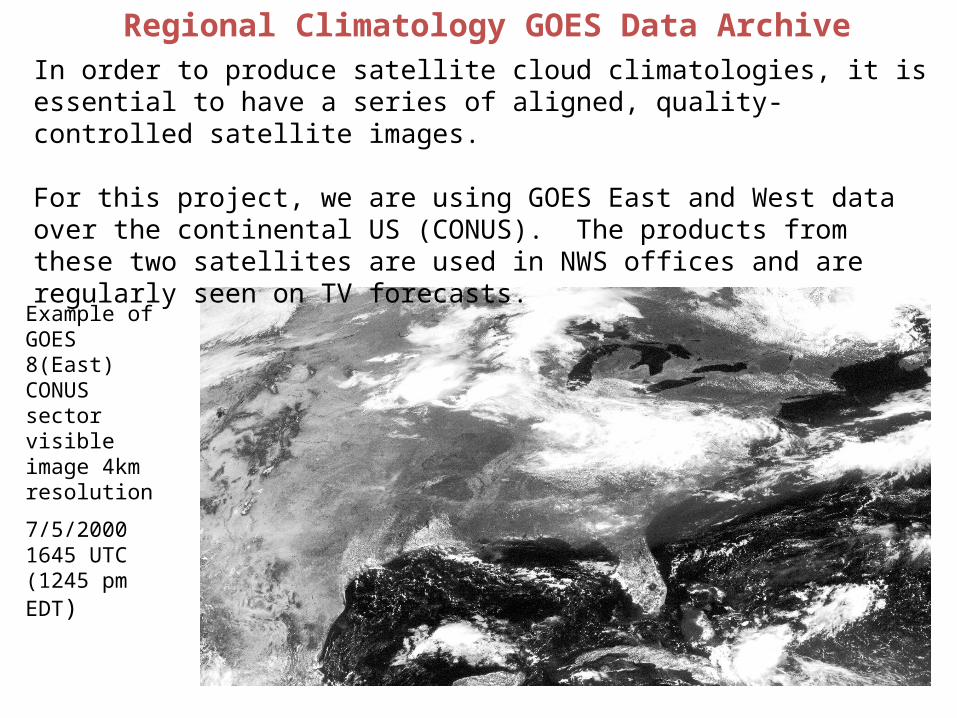
Regional Climatology GOES Data Archive

Example of GOES 8(East) CONUS sector visible image 4km resolution

7/5/2000 1645 UTC (1245 pm EDT)

In order to produce satellite cloud climatologies, it is essential to have a series of aligned, quality-controlled satellite images.

For this project, we are using GOES East and West data over the continental US (CONUS). The products from these two satellites are used in NWS offices and are regularly seen on TV forecasts.

Admittedly, the current geostationary GOES series does not have as many channels as the polar orbiters. However, the series’ ability to produce images every 30 minutes is ideal for studying weather and clouds that develop over the course of a day.

Example of GOES 11(West) CONUS sector visible image 4km resolution

8/4/2009 2100 UTC (2pm PDT)

The Imager on GOES produces five ‘channels’: visible, 3.9 m (near infrared(IR)), 6.7 m (water vapor), 10.7 m (thermal IR) and 12 m (split window IR). In later versions of the GOES series, the 12 m has been replaced with 13.3 m

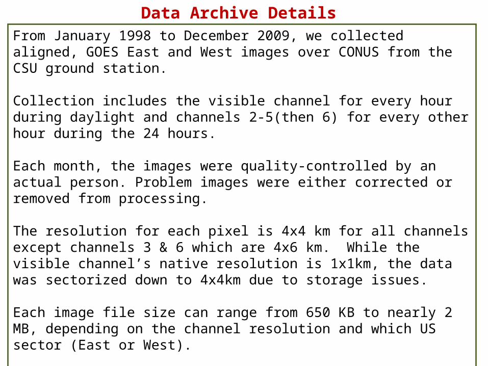
From January 1998 to December 2009, we collected aligned, GOES East and West images over CONUS from the CSU ground station.

Collection includes the visible channel for every hour during daylight and channels 2-5(then 6) for every other hour during the 24 hours.

Each month, the images were quality-controlled by an actual person. Problem images were either corrected or removed from processing.

The resolution for each pixel is 4x4 km for all channels except channels 3 & 6 which are 4x6 km. While the visible channel’s native resolution is 1x1km, the data was sectorized down to 4x4km due to storage issues.

Each image file size can range from 650 KB to nearly 2 MB, depending on the channel resolution and which US sector (East or West).

Monthly/hourly products include: cloud cleared background for all visible hours, minimum values for each channel, maximum values for each channel, cloud cover percent using a visible threshold method and cloud cover percent using a thermal IR threshold.

Data Archive Details

Producing Cloud Climatologies

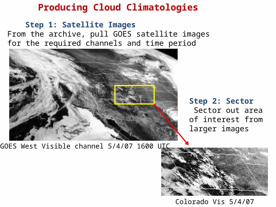
From the archive, pull GOES satellite images for the required channels and time period

Step 2: Sector Sector out area of interest from larger images

Colorado Vis 5/4/07 16UTC

GOES West Visible channel 5/4/07 1600 UTC

Step 1: Satellite Images

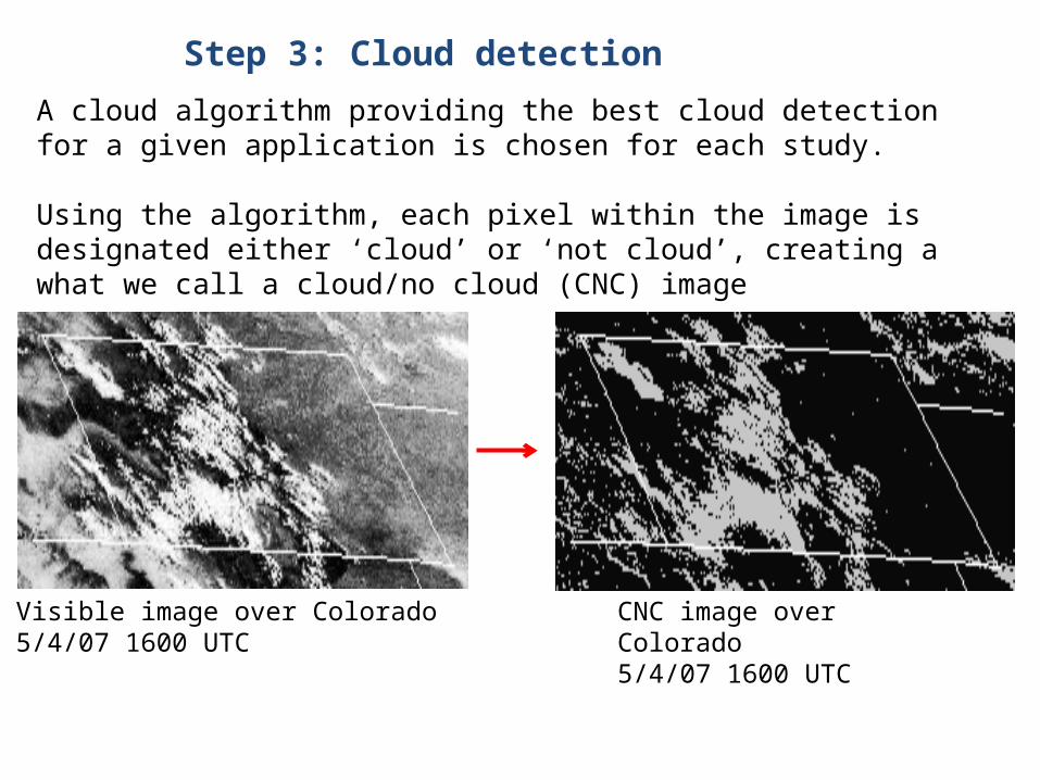
Step 3: Cloud detection

A cloud algorithm providing the best cloud detection for a given application is chosen for each study.

Using the algorithm, each pixel within the image is designated either ‘cloud’ or ‘not cloud’, creating a what we call a cloud/no cloud (CNC) image

Visible image over Colorado5/4/07 1600 UTC

CNC image over Colorado5/4/07 1600 UTC

Step 4: Determining Regimes

An important step is to decide how to divide up the data into regimes. There are two considerations – time and other meteorological parameters.

Most regional climatologies are divided into time of day, such as 1200 UTC, 1400 UTC, etc. However, they can also be divided into time before or after a meteorological event, such as 12 hours before the onset of high winds.

While general climatologies based solely on time can be useful, we’ve discovered that by pairing the satellite data with other meteorological data, more information about a given weather phenomena can be obtained.

So determining which set of meteorological variables to use to classify the satellite data can make a major difference in the results. In the past, wind speed and direction, depth of marine stratus layer at dawn, or the conditions leading to sea breeze development have been used.

Once regimes are chosen, the CNC images are matched with corresponding regimes.

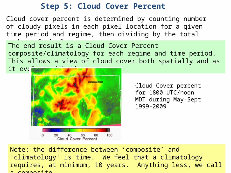
Step 5: Cloud Cover Percent

Cloud cover percent is determined by counting number of cloudy pixels in each pixel location for a given time period and regime, then dividing by the total number of pixels.

The end result is a Cloud Cover Percent composite/climatology for each regime and time period. This allows a view of cloud cover both spatially and as it evolves with time.

Note: the difference between ‘composite’ and ‘climatology’ is time. We feel that a climatology requires, at minimum, 10 years. Anything less, we call a composite.

Cloud Cover percent for 1800 UTC/noon MDT during May-Sept 1999-2009

Reading a Cloud Climatology

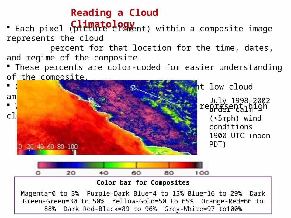
Each pixel (picture element) within a composite image represents the cloud percent for that location for the time, dates, and regime of the composite. These percents are color-coded for easier understanding of the composite. Cool colors (pinks and blues) represent low cloud amounts Warm colors (orange, reds, and black) represent high cloud amounts.

Color bar for Composites

Magenta=0 to 3% Purple-Dark Blue=4 to 15% Blue=16 to 29% Dark Green-Green=30 to 50% Yellow-Gold=50 to 65% Orange-Red=66 to 88% Dark Red-Black=89 to 96%

Grey-White=97 to100%

July 1998-2002under calm (<5mph) wind conditions1900 UTC (noon PDT)

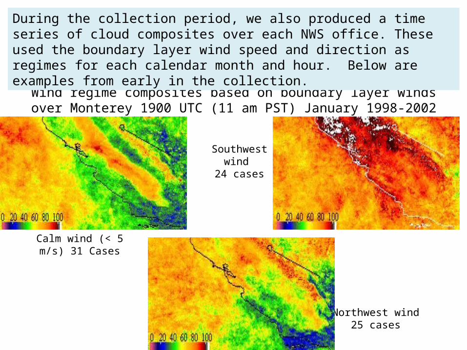
Calm wind (< 5 m/s) 31 Cases

Southwest wind

24 cases

Northwest wind 25 cases

Wind regime composites based on boundary layer winds over Monterey 1900 UTC (11 am PST) January 1998-2002

During the collection period, we also produced a time series of cloud composites over each NWS office. These used the boundary layer wind speed and direction as regimes for each calendar month and hour. Below are examples from early in the collection.

Marine Stratus/Fog Projects

For the Eureka and Monterey NWS offices, the marine stratus and fog that forms along the northwest Pacific coast is a major forecast challenge. The effects of the complex terrain features including various bays and coastal mountains ranges add to the challenge.

These clouds often persist for many days and are a major hazard to aviation and to travelers along the coast.

Forecasters are interested in the development, duration, and burn off rate of this marine stratus deck. All these factors have an impact on temperature, visibility, and sky cover forecasts.

Two sets of regional climatologies were developed with input from the Monterey and Eureka NWS offices. Each use different meteorological parameters to categorize and study marine stratus.

Motivation for National Weather Service

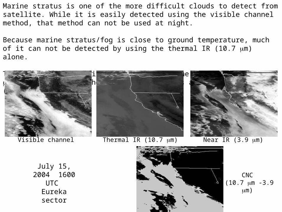
Marine stratus is one of the more difficult clouds to detect from satellite. While it is easily detected using the visible channel method, that method can not be used at night.

Because marine stratus/fog is close to ground temperature, much of it can not be detected by using the thermal IR (10.7 m) alone.

Thus, we use an algorithm that uses both the 10.7 m and the 3.9 m. However, this method does have problems at the terminators (sunrise/sunset)

July 15, 2004 1600 UTC

Eureka sector

Visible channel Thermal IR (10.7 m) Near IR (3.9 m)

CNC (10.7 m -3.9 m)

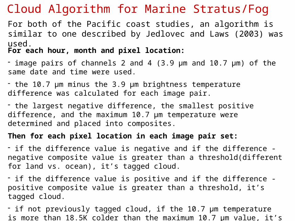
Cloud Algorithm for Marine Stratus/Fog

For each hour, month and pixel location:

- image pairs of channels 2 and 4 (3.9 μm and 10.7 μm) of the same date and time were used.

- the 10.7 μm minus the 3.9 μm brightness temperature difference was calculated for each image pair.

- the largest negative difference, the smallest positive difference, and the maximum 10.7 μm temperature were determined and placed into composites.

Then for each pixel location in each image pair set:

- if the difference value is negative and if the difference -negative composite value is greater than a threshold(different for land vs. ocean), it’s tagged cloud.

- if the difference value is positive and if the difference -positive composite value is greater than a threshold, it’s tagged cloud.

- if not previously tagged cloud, if the 10.7 μm temperature is more than 18.5K colder than the maximum 10.7 μm value, it’s tagged cloud.

- if it passes the three tests above, it’s classified as clear

For both of the Pacific coast studies, an algorithm is similar to one described by Jedlovec and Laws (2003) was used.

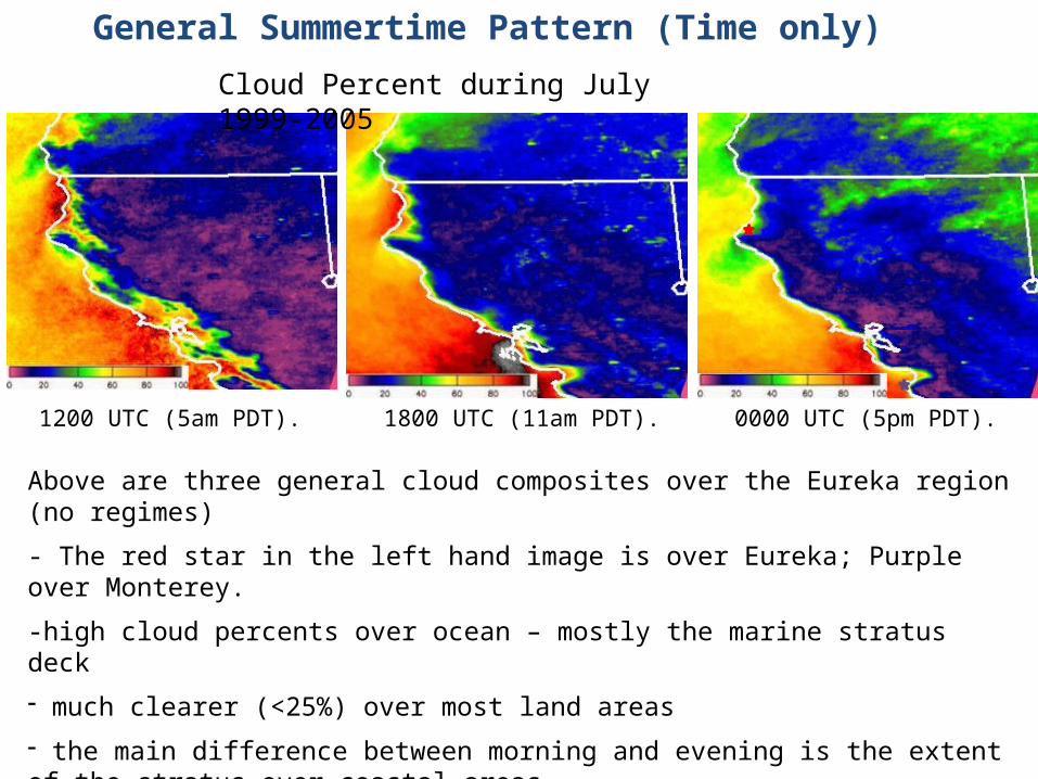
General Summertime Pattern (Time only)

Cloud Percent during July 1999-2005

1200 UTC (5am PDT). 1800 UTC (11am PDT). 0000 UTC (5pm PDT).

Above are three general cloud composites over the Eureka region (no regimes)

- The red star in the left hand image is over Eureka; Purple over Monterey.

-high cloud percents over ocean – mostly the marine stratus deck

- much clearer (<25%) over most land areas

- the main difference between morning and evening is the extent of the stratus over coastal areas.

Monterey, CA

The Monterey/San Francisco Bay area project was our first to examine marine stratus and fog. It was done in collaboration with Warren Blier and Walter Strach from the Monterey NWS office.

Marine stratus and fog is of huge interest for the office’s general and aviation forecasters for the reasons previously stated.

This study project was developed to both see if the cloud composites could provide them with additional information, and to test a general rule of thumb used in the office by the forecasters.

Introduction

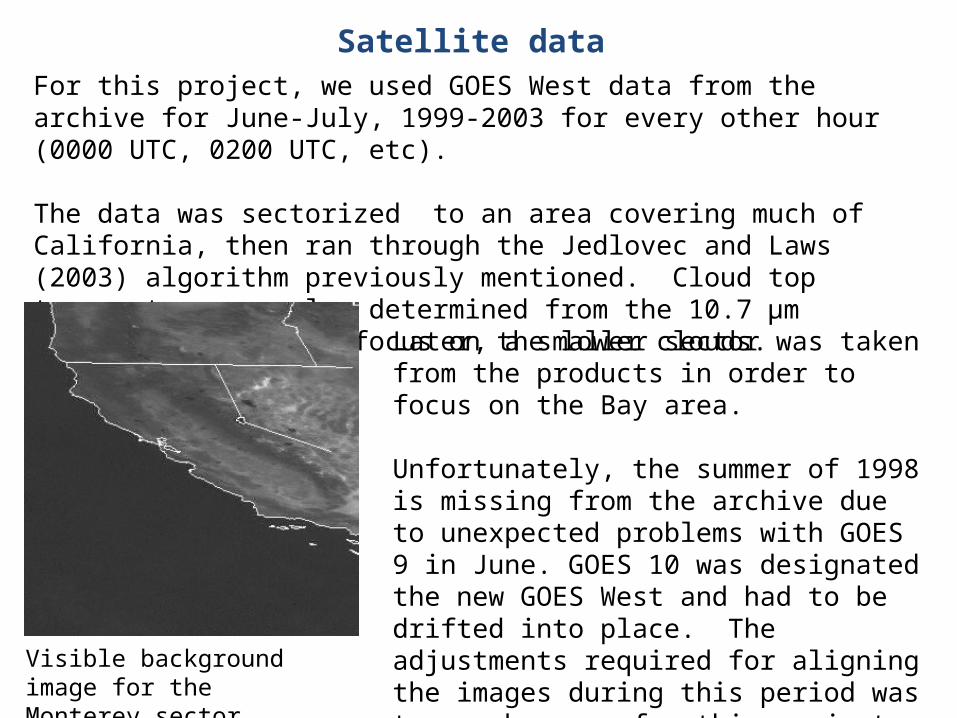
Satellite dataFor this project, we used GOES West data from the archive for June-July, 1999-2003 for every other hour (0000 UTC, 0200 UTC, etc).

The data was sectorized to an area covering much of California, then ran through the Jedlovec and Laws (2003) algorithm previously mentioned. Cloud top temperature was also determined from the 10.7 μm channel in order to focus on the lower clouds.

Visible background image for the Monterey sector

Later, a smaller sector was taken from the products in order to focus on the Bay area.

Unfortunately, the summer of 1998 is missing from the archive due to unexpected problems with GOES 9 in June. GOES 10 was designated the new GOES West and had to be drifted into place. The adjustments required for aligning the images during this period was too cumbersome for this project.

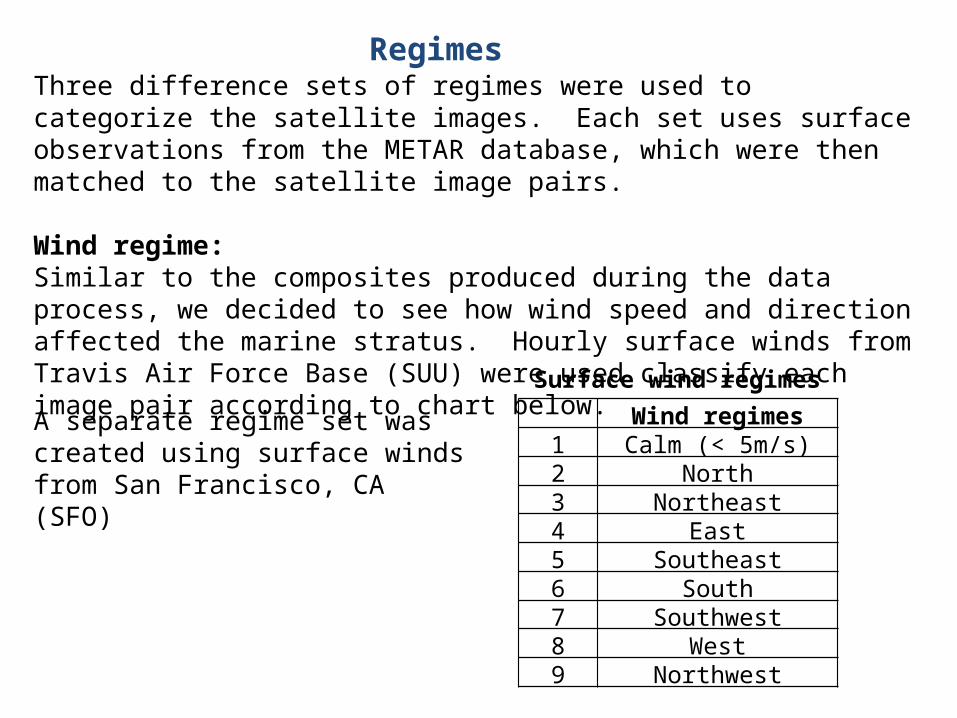
RegimesThree difference sets of regimes were used to categorize the satellite images. Each set uses surface observations from the METAR database, which were then matched to the satellite image pairs.

Wind regime:Similar to the composites produced during the data process, we decided to see how wind speed and direction affected the marine stratus. Hourly surface winds from Travis Air Force Base (SUU) were used classify each image pair according to chart below.

Wind regimes1 Calm (< 5m/s)2 North3 Northeast4 East5 Southeast6 South7 Southwest8 West9 Northwest

Surface wind regimes

A separate regime set was created using surface winds from San Francisco, CA (SFO)

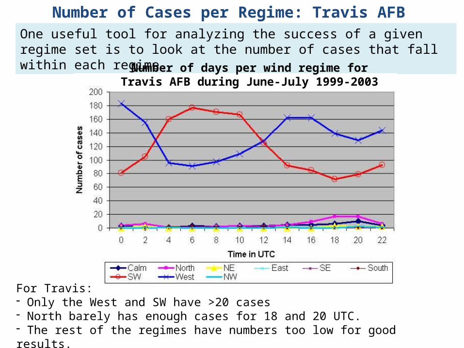
Number of Cases per Regime: Travis AFBOne useful tool for analyzing the success of a given regime set is to look at the number of cases that fall within each regime.

For Travis: - Only the West and SW have >20 cases - North barely has enough cases for 18 and 20 UTC.- The rest of the regimes have numbers too low for good results.

Number of days per wind regime for Travis AFB during June-July 1999-2003

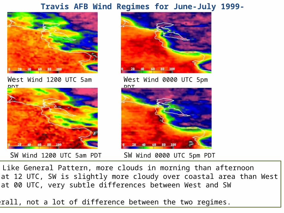
West Wind 0000 UTC 5pm PDT

Travis AFB Wind Regimes for June-July 1999-2003

West Wind 1200 UTC 5am PDT

SW Wind 1200 UTC 5am PDT SW Wind 0000 UTC 5pm PDT

- Like General Pattern, more clouds in morning than afternoon - at 12 UTC, SW is slightly more cloudy over coastal area than West - at 00 UTC, very subtle differences between West and SW

Overall, not a lot of difference between the two regimes.

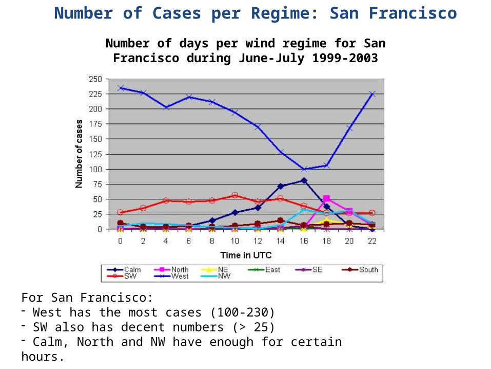
Number of days per wind regime for San Francisco during June-July 1999-2003

For San Francisco:- West has the most cases (100-230)- SW also has decent numbers (> 25)- Calm, North and NW have enough for certain hours.

Number of Cases per Regime: San Francisco

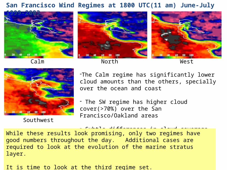
San Francisco Wind Regimes at 1800 UTC(11 am) June-July 1999-2003

Calm

Southwest

WestNorth

-The Calm regime has significantly lower cloud amounts than the others, specially over the ocean and coast

- The SW regime has higher cloud cover(>70%) over the San Francisco/Oakland areas

- Subtle differences in cloud coverage can also be seen with in the North and West wind cases

While these results look promising, only two regimes have good numbers throughout the day. Additional cases are required to look at the evolution of the marine stratus layer.

It is time to look at the third regime set.

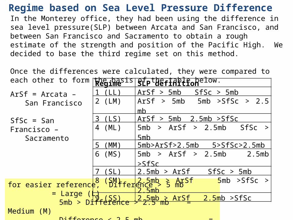
In the Monterey office, they had been using the difference in sea level pressure(SLP) between Arcata and San Francisco, and between San Francisco and Sacramento to obtain a rough estimate of the strength and position of the Pacific High. We decided to base the third regime set on this method.

Once the differences were calculated, they were compared to each other to form the basis of the table below.

for easier reference, Difference > 5 mb = Large (L) 5mb > Difference > 2.5 mb = Medium (M) Difference < 2.5 mb = Small (S)

Regime SLP definition1 (LL) ArSf > 5mb SfSc > 5mb2 (LM) ArSf > 5mb 5mb >SfSc > 2.5 mb3 (LS) ArSf > 5mb 2.5mb >SfSc4 (ML) 5mb > ArSf > 2.5mb SfSc > 5mb5 (MM) 5mb>ArSf>2.5mb 5>SfSc>2.5mb6 (MS) 5mb > ArSf > 2.5mb 2.5mb >SfSc7 (SL) 2.5mb > ArSf SfSc > 5mb8 (SM) 2.5mb > ArSf 5mb >SfSc > 2.5mb9 (SS) 2.5mb > ArSf 2.5mb >SfSc

ArSf = Arcata –San Francisco

SfSc = San Francisco –Sacramento

Regime based on Sea Level Pressure Difference

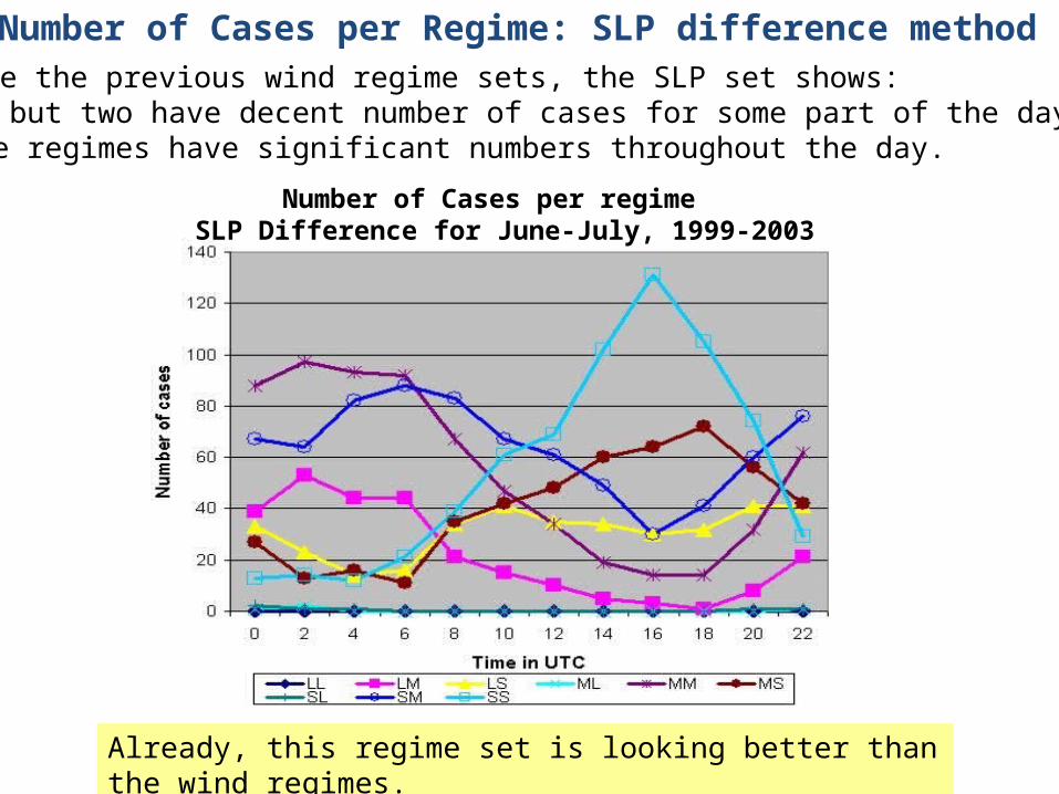
Number of Cases per regime SLP Difference for June-July, 1999-2003

Number of Cases per Regime: SLP difference methodUnlike the previous wind regime sets, the SLP set shows:- all but two have decent number of cases for some part of the day- five regimes have significant numbers throughout the day.

Already, this regime set is looking better than the wind regimes.

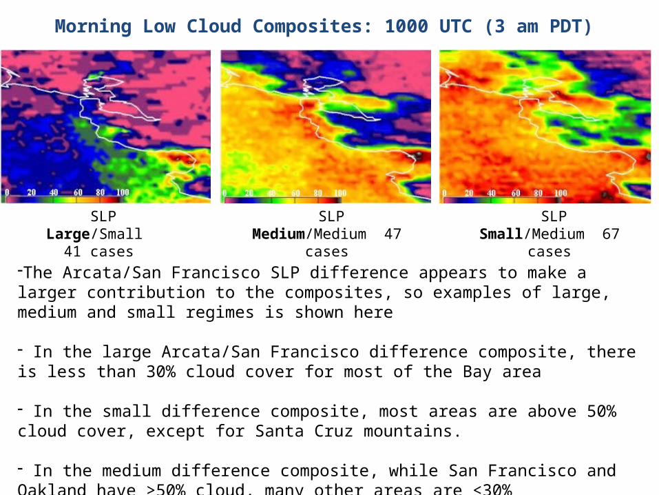
Morning Low Cloud Composites: 1000 UTC (3 am PDT)

SLP Large/Small 41 cases

SLP Medium/Medium 47 cases

SLP Small/Medium 67 cases

-The Arcata/San Francisco SLP difference appears to make a larger contribution to the composites, so examples of large, medium and small regimes is shown here

- In the large Arcata/San Francisco difference composite, there is less than 30% cloud cover for most of the Bay area

- In the small difference composite, most areas are above 50% cloud cover, except for Santa Cruz mountains.

- In the medium difference composite, while San Francisco and Oakland have >50% cloud, many other areas are <30%

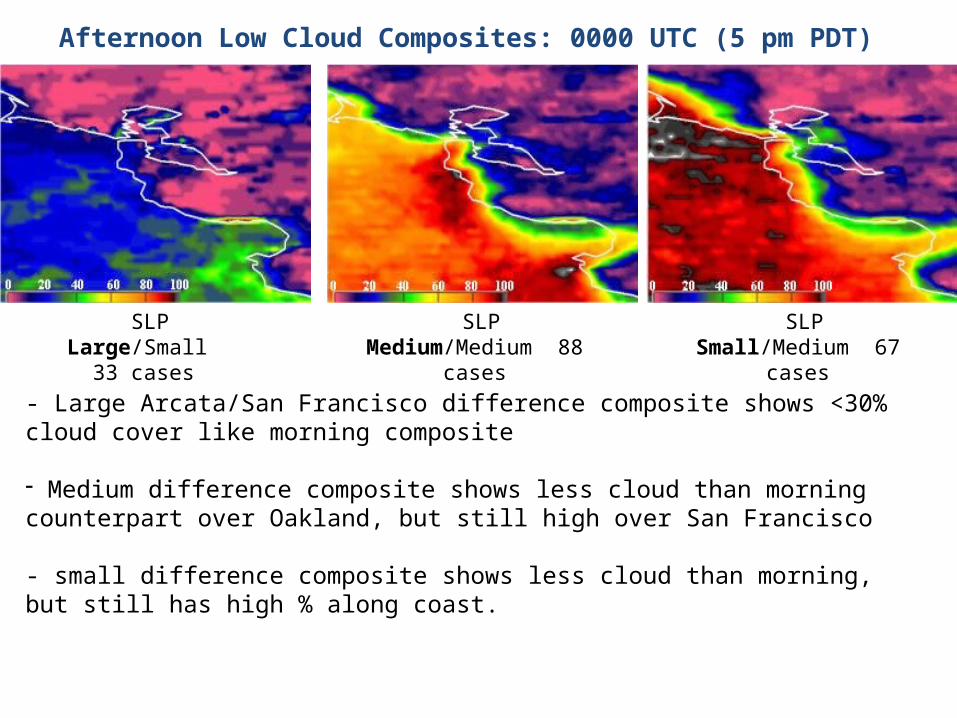
Afternoon Low Cloud Composites: 0000 UTC (5 pm PDT)

SLP Large/Small 33 cases

SLP Medium/Medium 88 cases

SLP Small/Medium 67 cases

- Large Arcata/San Francisco difference composite shows <30% cloud cover like morning composite

- Medium difference composite shows less cloud than morning counterpart over Oakland, but still high over San Francisco

- small difference composite shows less cloud than morning, but still has high % along coast.

Conclusions for Monterey Project

Cloud composites are shown to be a useful tool for examining local and regional meteorological events.

The San Francisco wind regime shows promise. However, lack of data in key time periods provides an incomplete view.

The SLP difference regimes show a lot of promise. Results seem to suggest more inland penetration of the marine stratus layer occurs when there is a weaker SLP pressure difference between Arcata and San Francisco. There are also significantly lower cloud amounts when the SLP pressure difference is large.

Eureka, CA

The Eureka project was started when Mel Nordquist, the SOO for the Eureka NWS office, contacted me. He had heard about the cloud climatologies and was interested in doing something similar for his area.

His idea was to look at depth of the marine stratus deck along their coast and to see if that was an indicator to how far inland the clouds extended and if it was a predictor to the burn off rate during the day.

Together with several of their office interns (Rebecca Mazur, Joseph Clark, Arlena Moses and Treena Hartley) and my (college and high school) student hourly workers, we were able to produce the following work.

Introduction

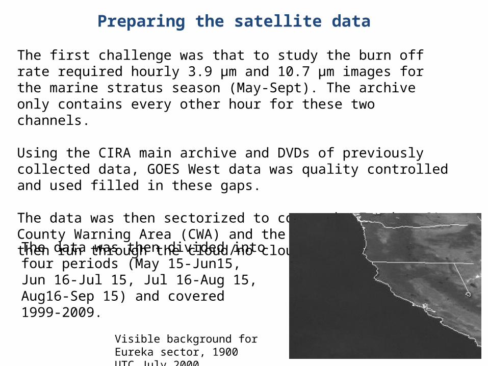
Preparing the satellite data

The first challenge was that to study the burn off rate required hourly 3.9 μm and 10.7 μm images for the marine stratus season (May-Sept). The archive only contains every other hour for these two channels.

Using the CIRA main archive and DVDs of previously collected data, GOES West data was quality controlled and used filled in these gaps.

The data was then sectorized to cover the Eureka, CA, County Warning Area (CWA) and the surrounding area, then run through the cloud/no cloud process.

The data was then divided into four periods (May 15-Jun15, Jun 16-Jul 15, Jul 16-Aug 15, Aug16-Sep 15) and covered 1999-2009.

Visible background for Eureka sector, 1900 UTC July 2000

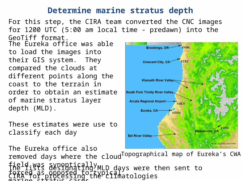
Determine marine stratus depthFor this step, the CIRA team converted the CNC images for 1200 UTC (5:00 am local time - predawn) into the GeoTiff format.

The Eureka office was able to load the images into their GIS system. They compared the clouds at different points along the coast to the terrain in order to obtain an estimate of marine stratus layer depth (MLD).

These estimates were use to classify each day

The Eureka office also removed days where the cloud field was synoptically forced as opposed to typical marine stratus cases.

Topographical map of Eureka’s CWA

The lists designating MLD days were then sent to CIRA for processing the climatologies

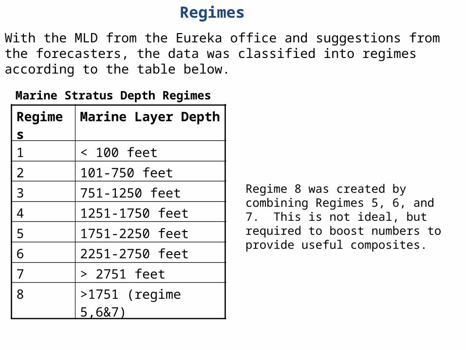
With the MLD from the Eureka office and suggestions from the forecasters, the data was classified into regimes according to the table below.

Regimes Marine Layer Depth

1 < 100 feet

2 101-750 feet

3 751-1250 feet

4 1251-1750 feet

5 1751-2250 feet

6 2251-2750 feet

7 > 2751 feet

8 >1751 (regime 5,6&7)

Regimes

Regime 8 was created by combining Regimes 5, 6, and 7. This is not ideal, but required to boost numbers to provide useful composites.

Marine Stratus Depth Regimes

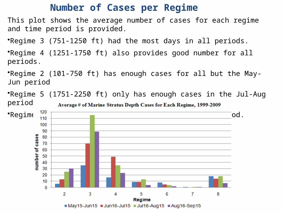
Number of Cases per RegimeThis plot shows the average number of cases for each regime and time period is provided.

•Regime 3 (751-1250 ft) had the most days in all periods.

•Regime 4 (1251-1750 ft) also provides good number for all periods.

•Regime 2 (101-750 ft) has enough cases for all but the May-Jun period

•Regime 5 (1751-2250 ft) only has enough cases in the Jul-Aug period.

•Regimes 6 and 7 do not have enough cases in any period.

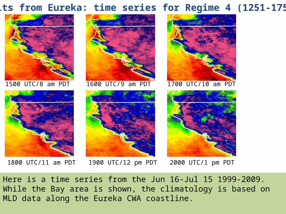
Results from Eureka: time series for Regime 4 (1251-1750 ft)

Here is a time series from the Jun 16-Jul 15 1999-2009. While the Bay area is shown, the climatology is based on MLD data along the Eureka CWA coastline.

Note the hourly reduction of the marine stratus along the coast.

1500 UTC/8 am PDT 1600 UTC/9 am PDT 1700 UTC/10 am PDT

1800 UTC/11 am PDT 1900 UTC/12 pm PDT 2000 UTC/1 pm PDT

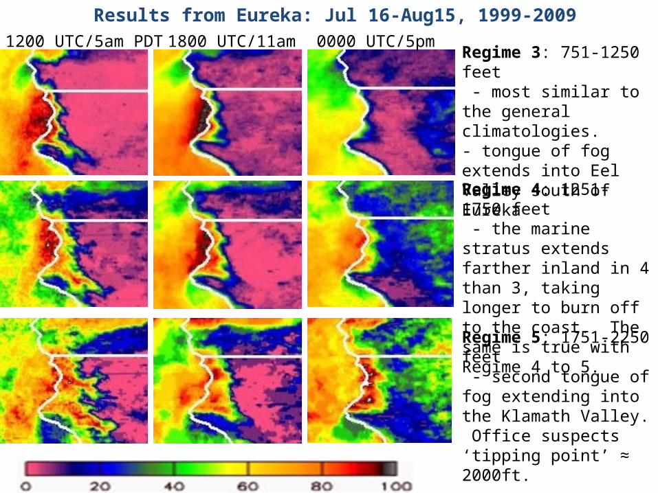
Results from Eureka: Jul 16-Aug15, 1999-2009

1200 UTC/5am PDT 1800 UTC/11am 0000 UTC/5pmRegime 3: 751-1250 feet - most similar to the general climatologies. - tongue of fog extends into Eel Valley south of Eureka

Regime 4: 1251- 1750 feet - the marine stratus extends farther inland in 4 than 3, taking longer to burn off to the coast. The same is true with Regime 4 to 5.

Regime 5: 1751-2250 feet - second tongue of fog extending into the Klamath Valley. Office suspects ‘tipping point’ ≈ 2000ft.

Comparison between observations and climatologiesStratus Event of Aug. 13, 2010

• PIREPs and visual spotter reports were used to establish the MLD. On this date, it is estimated to be 1000 ft or regime 3

•Fog product is used for 12 UTC and visible for 18 UTC.

•Spatial distribution is seen to correlate well.

•Through the use of GIS, more quantitative statistics for spatial correlation are planned

•The climatologies plan to be used as templates for Graphical Forecast Editor (GFE) to provide low level cloud grids.

Regime 3 climatology for Jul16-Aug15 at 12 UTC

Fog product at 12 UTC on August 13, 2010

Regime 3 climatology for Jul16-Aug15 at 18 UTC

Visible image at 18 UTC on August 13, 2010

SummaryFrom these examples, it has been shown that regional cloud climatologies can be a useful tool in studying and forecasting marine stratus and fog.

The climatologies are being validated and used in the Eureka NWS office.

When it comes to climatologies, the more data the better. Clouds and weather patterns are too variable to be captured within a couple of years.

Current plans are to include the fog data from the Eureka project in the fog database.

To learn more about the Eureka project and regional satellite climatologies, visit the websites at http://rammb.cira.colostate.edu/research/goes-r/proving_ground/cira_product_list/eureka_marine_stratus_cloud_climatologies.asp

http://rammb.cira.colostate.edu/research/satellite_climatologies/

A VISIT training session on this topic and other projects can be found at: http://rammb.cira.colostate.edu/training/visit/training_sessions/regional_satellite_cloud_composites_from_goes/

Combs, C.L., W. Blier, W. Strach, M., DeMaria, 2004: Exploring the timing of fog formation and dissipation over San Francisco Bay area using satellite cloud composites. Preprints, 13th Conf. Satellite Meteorology and Oceanography, Norfolk, VA, Amer. Meteor. Soc. P4.12.

Combs, C.L., R. Mazur, J. Clark, M. Norquist, and D. Molenar, 2010: An effort to improve marine stratus forecasts using satellite cloud climatologies for the Eureka, CA region. Preprints, 17th Conf Satellite Meteorology and Oceanography, Annapolis, MD, Amer. Meteor.Soc. P9.16.

Connell, B. H., K. J. Gould, and J. F. W. Purdom, 2001. High resolution GOES-8 visible and infrared cloud frequency composites over northern Florida during the summers 1996-1999. Wea. Forecasting, 16, 713- 724.

Jedlovec, G.J., and K. Laws, 2003: GOES cloud detection at the global hydrology and climate center. Preprints, 12th Conf. On Satellite Meteorology and Oceanography, Long Beach, CA, Amer. Meteor. Soc., poster P1.21.

Reinke, D. L., C. L. Combs, S. Q. Kidder, and T. H. Vonder Haar, 1992: Satellite cloud composite climatologies: A new high-resolution tool in Atmospheric research and Forecasting. Bull. Amer. Meteor. Soc. 73, 278 - 285.

References

THANK YOU!