Embed Size (px)
Citation preview
Software Framework for Collaborative Developmentof Nonlinear Dynamic Analysis Program
Jun PengStanford University
and
Kincho H. LawStanford University
Pacific Earthquake EngineeringResearch Center
PEER 2003/02SEPT. 2003
Software Framework for Collaborative Development of Nonlinear Dynamic Analysis Program
Jun Peng Department of Civil and Environmental Engineering
Stanford University
and
Kincho H. Law Department of Civil and Environmental Engineering
Stanford University
A report on research conducted under grant no. EEC-9701568 from the National Science Foundation:
PEER Report 2003/02 Pacific Earthquake Engineering Research Center
College of Engineering University of California, Berkeley
September 2003
iii
ABSTRACT
This report describes the research and prototype implementation of an Internet-enabled software
framework that facilitates the utilization and the collaborative development of a nonlinear
dynamic analysis program by taking advantage of object-oriented modeling, distributed
computing, database, and other advanced computing technologies. This new framework allows
users easy access to the analysis program and the analysis results by using a web browser or
other application programs, such as MATLAB. In addition, the framework serves as a common
finite element analysis platform for which researchers and software developers can build, test,
and incorporate new developments.
The collaborative software framework is built upon an object-oriented finite element
analysis program. The research objective is to enhance and improve the capability and
performance of the finite element program by seamlessly integrating legacy code and new
developments. Developments can be incorporated by directly integrating with the core as a local
module and/or by implementing as a remote service module. There are several approaches to
incorporate software modules locally, such as defining new subclasses, building interfaces and
wrappers, or developing a reverse communication mechanism. The distributed and collaborative
architecture also allows a software component to be incorporated as a service in a dynamic and
distributed manner. Two forms of remote element services, namely the distributed element
service and the dynamic shared library element service, are introduced in the framework to
facilitate the distributed usage and the collaborative development of a finite element program.
The collaborative finite element software framework also includes data and project
management functionalities. A database system is employed to store selected analysis results
and to provide flexible data management and data access. The Internet is utilized as a data
delivery vehicle, and a data query language is developed to provide an easy-to-use mechanism to
access the needed analysis results from readily accessible sources in a ready-to-use format for
further manipulation. Finally, a simple project management scheme is developed to allow the
users to manage and to collaborate on the analysis of a structure.
iv
ACKNOWLEDGMENTS
This report is based on a Ph.D. dissertation by the first author at Stanford University. The
research project was conducted at Stanford University from 1998–2002. The authors would like
to thank Dr. Frank McKenna and Professor Gregory L. Fenves of UC Berkeley for their
collaboration on and support of this research. They provided not only the source code of
OpenSees but also continuous support throughout the research. The linear sparse solver
SymSparse was developed by Dr. David Mackay of Intel Corporation, and the Lanczos solver for
generalized eigenvalue problem was implemented by Mr. Yang Wang of Stanford University.
We are also grateful to Mr. Ricardo Medina at Stanford University for providing the 18-story
one-bay frame analysis model, and to Dr. Zhaohui Yang, Mr. Yuyi Zhang, and Professors
Ahmed Elgamal and Joel Conte at the University of California, San Diego, for providing the
Humboldt Bay Middle Channel Bridge model.
This research was supported in part by the Pacific Earthquake Engineering Research
Center through the Earthquake Engineering Research Centers Program of the National Science
Foundation under award number EEC-9701568, and in part by NSF Grant Number CMS-
0084530. The Technology for Education 2000 equipment grant from Intel Corporation to
Professor Kincho H. Law of Stanford University provided the computers employed in this
research.
v
CONTENTS
ABSTRACT.................................................................................................................................. iii
ACKNOWLEDGMENTS ........................................................................................................... iv
TABLE OF CONTENTS ..............................................................................................................v
LIST OF FIGURES ..................................................................................................................... ix
LIST OF TABLES ....................................................................................................................... xi
1 INTRODUCTION .................................................................................................................1
1.1 Problem Statement ..........................................................................................................1
1.2 Related Research.............................................................................................................2
1.2.1 Object-Oriented Finite Element Programming ...................................................3
1.2.2 Distributed Object Computing ............................................................................5
1.2.3 Data Management in FEA Computing................................................................7
1.3 Report Outline.................................................................................................................9
2 OBJECT-ORIENTED FINITE ELEMENT PROGRAM AND MODULE INTEGRATION ..................................................................................................................13 2.1 Features of Object-Oriented Finite Element Programs.................................................14
2.1.1 Object-Oriented Programming..........................................................................14
2.1.2 Design and Implementation of Object-Oriented FEA Programs ......................17
2.1.3 OpenSees...........................................................................................................19
2.2 Direct Module Integration.............................................................................................22
2.2.1 Incorporating New Developments ....................................................................23
2.2.2 Linking Software Components .........................................................................25
2.2.2.1 Graph Representation of Matrices ......................................................26
2.2.2.2 Linking METIS Routines ...................................................................28
2.2.3 Integration of Legacy Applications...................................................................30
2.2.3.1 Procedures of Direct Solver SymSparse.............................................30
2.2.3.2 Integration of Direct Solver SymSparse .............................................32
2.3 Module Integration with Reverse Communication Interface........................................34
2.3.1 Reverse Communication Interface....................................................................35
2.3.2 Incorporating Eigensolvers with OpenSees ......................................................36
vi
2.4 Quality and Performance Measurements ......................................................................40
2.4.1 Comparison of Matrix Ordering Schemes ........................................................40
2.4.2 Performance Comparison of Linear Solvers .....................................................42
2.4.3 Comparison of Eigensolvers .............................................................................44
2.5 Summary .......................................................................................................................45
3 OPEN COLLABORATIVE SOFTWARE FRAMEWORK...........................................47
3.1 Overview of the Collaborative Framework...................................................................48
3.1.1 System Architecture ..........................................................................................49
3.1.2 Mechanics .........................................................................................................51
3.1.3 Modular Design.................................................................................................52
3.2 User Interfaces ..............................................................................................................54
3.2.1 OpenSees Tcl Input Interface............................................................................54
3.2.2 Web-Based User Interface ................................................................................58
3.2.2.1 Web-to-OpenSees Interaction.............................................................58
3.2.2.2 Servlet Server-to-OpenSees Interaction .............................................59
3.2.3 MATLAB-Based User Interface .......................................................................61
3.2.3.1 Network Communication....................................................................62
3.2.3.2 Data Processing ..................................................................................63
3.3 Example ........................................................................................................................65
3.3.1 Sample Web-Based Interface............................................................................66
3.3.2 Sample MATLAB-Based Interface...................................................................69
3.4 Summary .......................................................................................................................70
4 INTERNET-ENABLED SERVICE INTEGRATION AND COMMUNICATION .....73
4.1 Registration and Naming Service .................................................................................75
4.2 Distributed Element Services........................................................................................78
4.2.1 Mechanics .........................................................................................................78
4.2.2 Interaction with Distributed Services................................................................83
4.2.3 Implementation .................................................................................................86
4.3 Dynamic Shared Library Element Services ..................................................................88
4.3.1 Static Library vs. Shared Library ......................................................................88
4.3.2 Mechanics .........................................................................................................89
4.3.3 Implementation .................................................................................................91
vii
4.4 Application....................................................................................................................94
4.4.1 Example Test Case............................................................................................94
4.4.2 Performance of Online Element Services .........................................................97
4.5 Summary and Discussion..............................................................................................99
5 DATA ACCESS AND PROJECT MANAGEMENT ....................................................101
5.1 Multitiered Architecture..............................................................................................102
5.2 Data Storage Scheme ..................................................................................................105
5.2.1 Selective Data Storage ....................................................................................107
5.2.2 Object Serialization.........................................................................................109
5.2.3 Sampling at a Specified Interval .....................................................................112
5.3 Data Representation ....................................................................................................114
5.3.1 Data Modeling.................................................................................................115
5.3.2 Project-Based Data Storage ............................................................................117
5.3.3 Data Representation in XML ..........................................................................119
5.4 Data Query Processing................................................................................................123
5.4.1 Data Query Language .....................................................................................124
5.4.2 Data Query Interfaces .....................................................................................126
5.5 Applications ................................................................................................................127
5.5.1 Example 1: Eighteen-Story One-Bay Frame Model .......................................128
5.5.2 Example 2: Humboldt Bay Middle Channel Bridge Model............................130
5.5.2.1 Project Management .........................................................................132
5.5.2.2 Data Storage and Data Access..........................................................134
5.6 Summary and Discussion............................................................................................137
6 SUMMARY AND FUTURE DIRECTIONS ..................................................................139
6.1 Summary .....................................................................................................................139
6.2 Future Directions.........................................................................................................141
REFERENCES...........................................................................................................................145
ix
LIST OF FIGURES
Figure 2.1 Class abstraction in OpenSees (courtesy of McKenna) ...........................................20
Figure 2.2 Class diagram for OpenSees analysis framework (courtesy of McKenna)..............22
Figure 2.3 Pseudo-code for getTangentStiff method of QuadEightElement class ....................25
Figure 2.4 Example of CSR storage for matrix structure ..........................................................27
Figure 2.5 Class interface for the MetisPartitioner class ...........................................................28
Figure 2.6 Pseudo-code for partition method of MetisPartitioner class ....................................29
Figure 2.7 Pseudo-code for incorporating METIS_NodeND method.......................................29
Figure 2.8 Interface for SymSparseLinSOE class .....................................................................33
Figure 2.9 Control flow of integrating the SymSparse linear solver .........................................34
Figure 2.10 Class diagram for eigenvalue analysis in OpenSees ................................................37
Figure 2.11 Linking ARPACK through reverse communication interface .................................39
Figure 2.12 Quality comparison of different matrix ordering schemes.......................................41
Figure 2.13 Performance comparison for different linear solvers ...............................................43
Figure 3.1 The collaborative system architecture......................................................................50
Figure 3.2 Mechanics of the collaborative framework..............................................................52
Figure 3.3 Modules of the collaborative system........................................................................53
Figure 3.4 Three-truss example (from McKenna and Fenves 2001).........................................56
Figure 3.5 The interaction diagram for the web-based interface...............................................59
Figure 3.6 Interaction diagram for the MATLAB-based interface............................................63
Figure 3.7 Array representations in Java and MATLAB ..........................................................64
Figure 3.8 Example model and Northridge earthquake record..................................................66
Figure 3.9 Part of Tcl input file for example model ..................................................................67
Figure 3.10 Sample web pages generated on the client site ........................................................68
Figure 3.11 Sample MATLAB-based user interface ...................................................................70
Figure 4.1 Registering and resolving names in RANS..............................................................75
Figure 4.2 Schema of the ServiceInfo table...............................................................................76
Figure 4.3 Interface for the RANS class....................................................................................77
Figure 4.4 Purpose of JNI (from Stearns 2002).........................................................................82
Figure 4.5 Mechanics of the distributed element service ..........................................................82
x
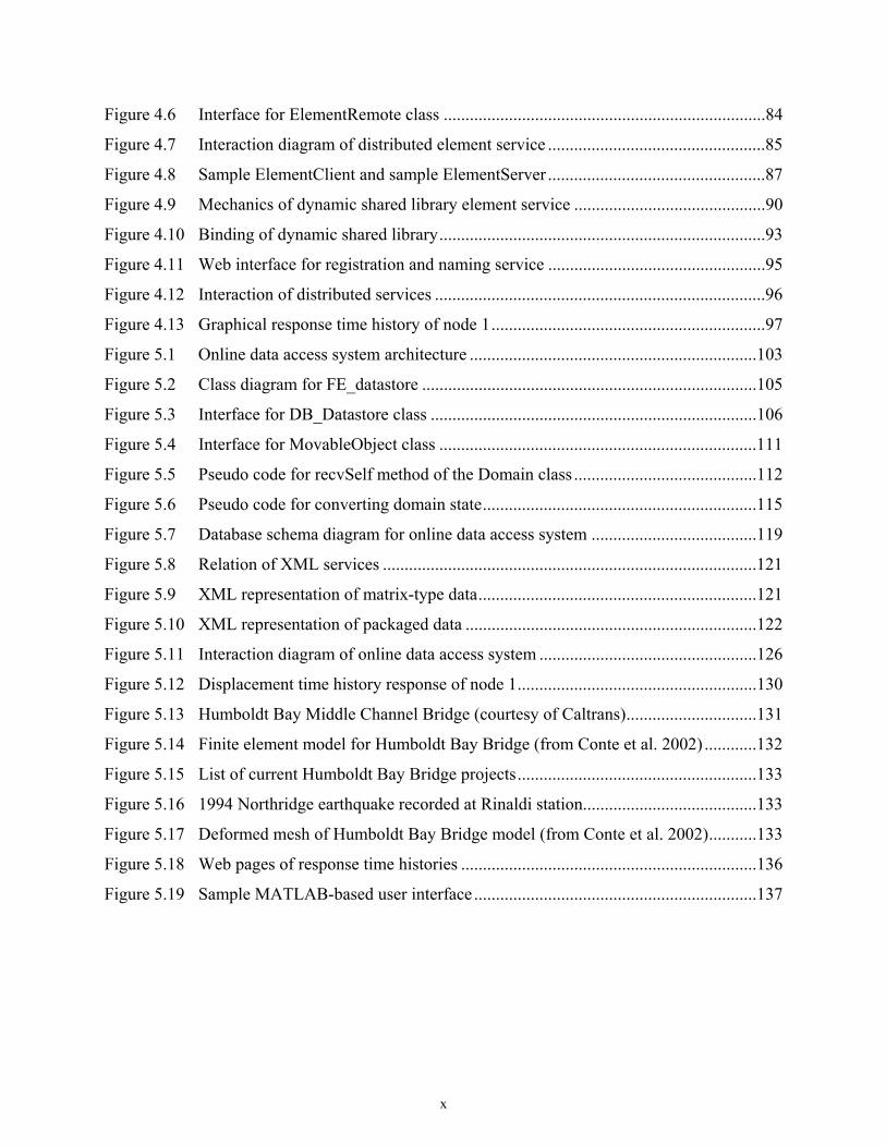
Figure 4.6 Interface for ElementRemote class ..........................................................................84
Figure 4.7 Interaction diagram of distributed element service ..................................................85
Figure 4.8 Sample ElementClient and sample ElementServer ..................................................87
Figure 4.9 Mechanics of dynamic shared library element service ............................................90
Figure 4.10 Binding of dynamic shared library...........................................................................93
Figure 4.11 Web interface for registration and naming service ..................................................95
Figure 4.12 Interaction of distributed services ............................................................................96
Figure 4.13 Graphical response time history of node 1...............................................................97
Figure 5.1 Online data access system architecture ..................................................................103
Figure 5.2 Class diagram for FE_datastore .............................................................................105
Figure 5.3 Interface for DB_Datastore class ...........................................................................106
Figure 5.4 Interface for MovableObject class .........................................................................111
Figure 5.5 Pseudo code for recvSelf method of the Domain class ..........................................112
Figure 5.6 Pseudo code for converting domain state...............................................................115
Figure 5.7 Database schema diagram for online data access system ......................................119
Figure 5.8 Relation of XML services ......................................................................................121
Figure 5.9 XML representation of matrix-type data................................................................121
Figure 5.10 XML representation of packaged data ...................................................................122
Figure 5.11 Interaction diagram of online data access system ..................................................126
Figure 5.12 Displacement time history response of node 1.......................................................130
Figure 5.13 Humboldt Bay Middle Channel Bridge (courtesy of Caltrans)..............................131
Figure 5.14 Finite element model for Humboldt Bay Bridge (from Conte et al. 2002) ............132
Figure 5.15 List of current Humboldt Bay Bridge projects.......................................................133
Figure 5.16 1994 Northridge earthquake recorded at Rinaldi station........................................133
Figure 5.17 Deformed mesh of Humboldt Bay Bridge model (from Conte et al. 2002)...........133
Figure 5.18 Web pages of response time histories ....................................................................136
Figure 5.19 Sample MATLAB-based user interface .................................................................137
xi
LIST OF TABLES
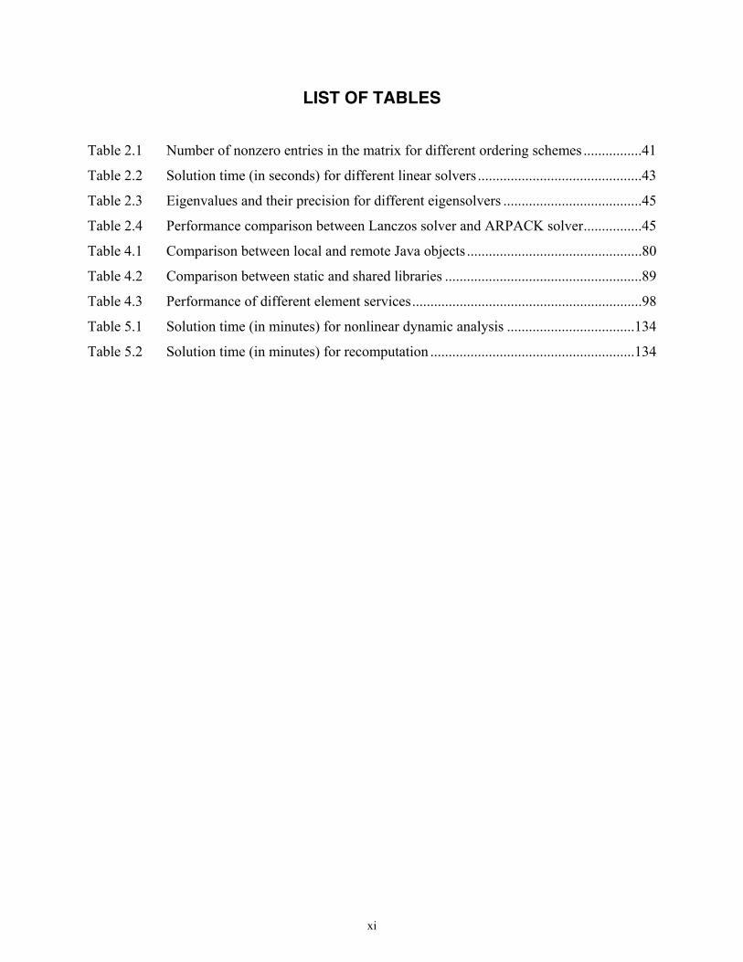
Table 2.1 Number of nonzero entries in the matrix for different ordering schemes ................41
Table 2.2 Solution time (in seconds) for different linear solvers .............................................43
Table 2.3 Eigenvalues and their precision for different eigensolvers ......................................45
Table 2.4 Performance comparison between Lanczos solver and ARPACK solver................45
Table 4.1 Comparison between local and remote Java objects ................................................80
Table 4.2 Comparison between static and shared libraries ......................................................89
Table 4.3 Performance of different element services...............................................................98
Table 5.1 Solution time (in minutes) for nonlinear dynamic analysis ...................................134
Table 5.2 Solution time (in minutes) for recomputation ........................................................134
1 Introduction
1.1 PROBLEM STATEMENT
It is well recognized that a significant gap exists between the advances in computing
technologies and the state of practice in structural engineering software development. Practicing
engineers today typically perform finite element structural analyses on a dedicated computer
using the developments offered by a single finite element analysis (FEA) program. Typically, a
finite element software package is developed by an individual organization and bundles all the
procedures and program kernels.
As technologies and structural theories continue to advance, structural analysis software
packages need to be able to accommodate new developments in element formulation, material
relations, analysis algorithms, solution strategies, and computing environments. The need to
develop and maintain large complex software systems in a dynamic environment has driven
interest in new approaches to finite element analysis software design and development. Object-
oriented design principles and programming can be utilized in finite element software
development to support better data encapsulation and to facilitate code reuse. However, most
existing object-oriented finite element programs remain rigidly structured. Extending and
upgrading these programs to incorporate new developments and legacy applications remain
difficult tasks. Moreover, there is no easy way to access computing resources and finite element
analysis services distributed in a remote site.
With the advances of computing facilities and the development of communication
networks in which the computing resources are connected and shared, the programming
environment has migrated from relying on a single and local computing environment to
developing software in a distributed and global environment. With the maturation of information
and communication technologies, the concept of building collaborative systems to distribute the
services over the Internet is becoming a reality (Han et al. 1999). Following this idea, we have
2
designed a prototype Internet-enabled collaborative framework for the usage and development of
a finite element analysis program. The collaborative software framework is built upon an object-
oriented finite element core program. The collaborative framework is designed to enhance and
improve the capability and performance of the finite element program by seamlessly integrating
legacy code and new developments. Developments can be incorporated by directly integrating
with the core as a local module and/or by implementing as a remote service module. The
Internet provides many possibilities for enhancing the distributive and collaborative software
development and utilization. By means of the Internet as a communication channel, which
supports standard communication protocols and network transparency, the collaborative
framework gives the users the ability to pick and choose the most appropriate methods and
software components for solving a problem.
To support collaboration among software developers and engineering users, the finite
element software framework also includes data and project management functionalities. A
database system is employed to store selected analysis results and to provide flexible data
management and data access. The Internet is utilized as a data delivery vehicle, and a data query
language is developed to provide an easy-to-use mechanism to access the needed analysis results
from readily accessible sources in a ready-to-use format for further manipulation. Finally, a
simple project management scheme is developed to allow the users to manage and to collaborate
on projects. Access control and revision control capabilities are integrated with the project
management system.
1.2 RELATED RESEARCH
The Internet-enabled collaborative software framework is based on an object-oriented finite
element analysis program. Distributed and collaborative computing is utilized in the framework
to allow an element service to be distributed over the Internet. A database is linked with the
software framework to provide persistent data storage and to facilitate data and project
management. This section presents an overview of some work related to this research effort,
including object-oriented finite element programs, distributed object computing, and data
management in finite element programs.
3
1.2.1 Object-Oriented Finite Element Programming
Most existing finite element software packages are developed in procedural-based programming
languages. These packages are normally monolithic and difficult for a programmer to maintain
and extend, though some of them are quite rich in terms of functionality. Extensibility usually
requires access to and manipulation of internal data structures. Due to the lack of data
encapsulation and protection, small changes in one piece of code can ripple through the rest of
the software system. For example, to add a new element to an existing procedural-based finite
element analysis software package, the programmer is usually required to specify, at the element
level, the memory pointers to global arrays. Exposing such unnecessary implementation details
increases the software complexity and adds a burden to a programmer. Even worse, any change
to these global data structures to accommodate new functionalities will require the
implementation of other elements to be changed. Therefore, such access may compromise the
reliability and integrity of the system. Furthermore, these packages do not provide a set of
crisply defined high-level abstraction or software components by which a programmer can
construct new applications to meet new functional requirements. For example, it is very difficult
to extend an existing linear static analysis program to geometric nonlinear or material nonlinear
transit analysis. It is difficult for researchers to test new algorithms in existing structural
engineering software. Few existing structural analysis programs offer the test-bed capabilities
for rapid prototyping due to the lack of high-level reusable components and their severe inherent
limitations in maintainability and extendibility.
Object-oriented design principles and programming techniques can be utilized in finite
element analysis programs to support better data encapsulation and to facilitate code reuse. A
number of object-oriented finite element program design and implementations have been
presented in the literature over the past decade (Commend and Zimmermann 2001; McKenna
1997; Miller 1991; among many others). Object-oriented finite element analysis packages,
particularly those written in C++, have been shown to have comparable performance to their
procedural-based counterparts and still provide the maintainability and extendibility essential for
modern-day software packages (Dubois-Pelerin and Zimmermann 1993; McKenna 1997; Rucki
and Miller 1996). The flexibility and extendibility of these packages are partly due to the object-
oriented support of encapsulation, inheritance, and polymorphism. There are three essential
4
steps in the development of object-oriented systems: identification of the classes, specification of
the class interfaces, and implementation.
Much of the early work concentrated on fairly straightforward implementations of FEM
in an object-oriented programming language — separate objects were created for elements,
nodes, loads, materials, degrees of freedom, etc. (Forde et al. 1990; Mackie 1992; Zimmermann
et al. 1992). Some work has been devoted to using object-oriented design to carry out complex
algorithms. The technique has been applied to many application areas including stress analysis
(Dubois-Pelerin and Zimmermann 1993; Kong and Chen 1995; Lu et al. 1994), hypersonic shock
waves (Budge and Peery 1993), structural dynamics (Archer 1996; Pidaparti and Hudli 1993),
shell structures (Ohtsubo et al. 1993), nonlinear plastic strain (Mentrey and Zimmermann 1993),
and electromagnetics (Silva et al. 1994). Algorithms that are difficult to program using
procedural languages (e.g., Fortran) have become easier in object-oriented programming
languages because of the richer data structures that can be created. A particularly interesting
application used objects to represent substructures (Ju and Hosain 1994). The application was
applied to repetitive structures, and this enabled the user to create the mesh easily by using a
series of copy, translation, and reflection operations. Eyheramendy and Zimmermann (1994)
used objects to develop a system that enabled the underlying mathematics of finite element
method to be represented.
There are several popular object-oriented programming languages such as Smalltalk,
C++, and Java. C++ is by far the most popular programming language for implementing object-
oriented finite element analysis programs. C++ was chosen because of its availability,
popularity, efficiency, and built-in libraries. One of the appealing features of C++ is that it
provides object-oriented capabilities as well as C functional elements. This hybrid language
feature helps to make C++ applications efficient. If implemented properly, C++ applications
tend to be more efficient than pure object-oriented languages (e.g., Smalltalk, Java, etc.) and
better suited to solve numerical problems arising in engineering applications. Moreover, most of
the C++ compilers provide easy calls to Fortran routines. This is an important advantage,
because it enables the reuse of many efficient Fortran subprograms. Another powerful feature of
C++ is the concept of dynamic binding of functions. It supports the mechanism of
polymorphism and is activated by adding the keyword virtual in a function definition. This
keyword notifies the compiler to decide during the runtime which function should be called. The
dynamic binding of functions makes the programs more flexible and also facilitates code reuse.
5
Finally, most of the C++ compilers provide an array of class libraries, which can solve many
implementation details at the lower class libraries. They shift the programmer’s efforts to a
higher-level abstraction, focusing on the overall organization and design of the program. Typical
class libraries include classes for string and input/output operations, as well as container classes
for storing and managing data.
1.2.2 Distributed Object Computing
Distributed object computing extends an object-oriented programming system by allowing
objects to be distributed across a heterogeneous network, so that each of these distributed object
components can interoperate as a unified system. These objects may be distributed on different
computers throughout a network, living within their own address space outside of an application,
and yet appear as though they are local to a central application. The basic extension for a
distributed object-oriented system is to provide remote procedure calls from a thread on one
machine to an object on another machine, using the same basic syntax and semantics as a local
call. A key property of distributed object computing is dispatching on the object first, rather than
binding to a particular procedure. Dispatching on the object allows there to be multiple
simultaneous different implementations.
Three of the most popular distributed object paradigms are Object Management Group’s
(OMG) Common Object Request Broker Architecture (CORBA) (Otte et al. 1996; Pope 1998),
Microsoft’s Distributed Component Object Model (DCOM) (Eddon and Eddon 1998), and Sun
Microsystems’ Java Remote Method Invocation (RMI) (Pitt and McNiff 2001). The following
gives a brief overview of these three distributed object computing technologies. A detailed
comparison of CORBA, DCOM and Java RMI has been discussed in Raj (1998).
The Common Object Request Broker Architecture (CORBA) is a source interface
standard being promoted by the Object Management Group (OMG), an industry standard
consortium. While the traditional objects reside in a single computer (within a single process or
multiple processes), distributed objects may reside in several nodes in a network. Robust
distributed objects may be written in different languages, and can be compiled by different
compilers while they communicate with each other via standardized protocols embodied by
middleware (Lewandowski 1998). Everything in the CORBA architecture depends on an Object
6
Request Broker (ORB). The ORB acts as a central object registry where each CORBA object
interacts transparently with other CORBA objects located either locally or remotely. CORBA
relies on a protocol called the Internet Inter-ORB Protocol (IIOP) for remote objects. Each
CORBA server object has an interface and exposes a set of methods. To request a service, a
CORBA client acquires an object reference to a CORBA server object. The client can make
method calls on the object reference as if the CORBA server object resides in the client’s address
space. The ORB is responsible for finding the CORBA object’s implementation, preparing it to
receive requests, communicating requests to it, and carrying the reply back to the client. A
CORBA object interacts with the ORB either through the ORB interface or through an object
adapter. Since CORBA is just a specification, it can be used on diverse operating system
platforms as long as there is an ORB implementation for that platform. The distributed objects
in the CORBA environment can be implemented in various programming languages, such as
C/C++ (Henning and Vinoski 1999) or Java (Orfali and Harkey 1998).
The Microsoft DCOM, extended from Component Object Model (COM) and more
recently in COM+, provides a distributed object framework as an extension of the OLE (Object
Linking and Embedding) facility. OLE allows objects to be linked by reference between types of
documents and objects to be embedded in other objects. DCOM supports remote objects by
running on a protocol called the Object Remote Procedure Call (ORPC). The ORPC layer is
built on top of standard remote procedure call (RPC) and interacts with COM’s runtime services.
A DCOM server is a body of code that is capable of serving up objects of a particular type at
runtime. Each DCOM server object can support multiple interfaces each representing a different
behavior of the object. A DCOM client class calls into the exposed methods of a DCOM server
by acquiring a pointer to one of the server object’s interfaces. The client object then starts
calling the server object’s exposed methods through the acquired interface pointer as if the server
object resides in the client’s address space. Since the COM specification is at the binary level, it
allows DCOM server components to be written in diverse programming languages like C++,
Java, and Visual Basic, etc. As long as a platform supports COM services, DCOM can be used
on that platform. DCOM is heavily used on the Microsoft Windows platform.
Java RMI relies on a protocol called the Java Remote Method Protocol (JRMP). Java
relies heavily on Java Object Serialization, which allows objects to be marshaled (or transmitted)
as a byte stream. Since Java Object Serialization is specific to Java, both the Java RMI server
object and the client object have to be written in Java. Each RMI server object defines an
7
interface which can be used to access the server object outside of the current Java Virtual
Machine (JVM) and on another machine's JVM. The interface exposes a set of methods that are
indicative of the services offered by the server object. For a client to locate a server object for
the first time, RMI depends on a registration and naming mechanism called an RMI Registry that
runs on the Server machine and holds information about available server objects. A RMI client
acquires an object reference to a JRMI server object by doing a lookup for a server object
reference and invokes methods on the server object as if the RMI server object resides in the
client's address space. RMI server objects are named using Uniform Resource Locator (URLs)
and for a client to acquire a server object reference, the client should specify the URL of the
server object similar to the URL for a HTML page. Since RMI relies on Java, it can be used on
diverse operating system platforms from mainframes to UNIX workstations to Windows
machines and handheld devices, as long as there is a Java Virtual Machine (JVM)
implementation for that platform.
The architectures of CORBA, DCOM and Java RMI provide mechanisms for transparent
invocation and accessing of remote distributed objects. Though the mechanisms that they
employ to achieve distributed computing may be different, the approach that each of them takes
is more or less similar.
1.2.3 Data Management in FEA Computing
The importance of a data management system in scientific and engineering computing has been
recognized for more than thirty years. Techniques for general data management were gradually
making inroads in scientific computing during the 1970s. This development paralleled in many
ways the rapid acceptance of the centralized database concept in business-oriented processing.
However, engineering data manipulation systems faced a specialized environment with its own
set of operational requirements. To present the specialized environment and operational
requirements of engineering data management systems, Felippa (1979, 1980, and 1982)
published a series of three papers on database usage in scientific computing. These papers
reviewed general features of scientific data management from a functional standpoint, including
the description of a database-linked engineering analysis system, the organization of a database
system, and the program operational compatibility. The general data structures and program
8
architecture were also presented, together with the issues regarding implementation and
deployment. Blackburn et al. (1983) described a relational database (RDB) management system
for computer-based integrated design, including application to the analysis of various structures
to demonstrate and evaluate the ability of an RDB system to store, retrieve, query, modify, and
manipulate data. All these papers emphasized the importance of centralized data management
for large-scale computing. Two factors that determined the favor of centralized scientific data
management were the sheer growth of large-scale engineering analysis codes to the point of
incipient instability as regards to propagation of local program errors, and the appearance of
integrated program networks that share a common project database. Centralized data
management was most effective when used in conjunction with a highly modular, structured
program architecture (Felippa 1980).
The role of databases as repositories of information (data) highlighted the importance of
data structures. The component data elements of data structures could be either atomic (i.e., non-
decomposable) or data structures themselves. The relationships between these component data
elements constitute the structure and have implications for the functions of the data structure
(Anumba 1996). Several general approaches and models for organizing the data have been
developed. They are the hierarchical approach, the network approach, the relational approach,
and the object-oriented approach. The hierarchical approach and the network approach are the
traditional means of organizing data and their relationships. The relational model has been
adopted in several finite element programs (Blackburn et al. 1983; Rajan and Bhatti 1986; Yang
1992). The object-oriented approach is the foundation for many object-oriented database
management systems, such as EXODUS (Carey et al. 1990), which is an extensible database
system to facilitate the fast development of high-performance, application-specific database
systems. No matter which data model is used, data structures need to be self-describable
(Felippa 1979). For practical reasons we can generally exclude the naïve approach of forcing
every program component to agree on a unified data structure. The next best thing is to require
each program to label its output data, i.e., to attach a descriptive label to each data structure that
would be saved in the database. Such tags can then be examined by the control structure of other
programs and appropriate actions can be taken.
Presently, the state of practice for data management in finite element analysis (FEA)
programs still relies mainly on file systems. To facilitate the sharing of information, loosely-
coupled systems could talk to each other through the same file system. However, data placed by
9
an application program into the file system may well not be acceptable to another program
because of format incompatibility. To tackle this problem, Yang (1992) defined a standard file
format for the analysis data, called the universal file (UF). Two interfaces have been proposed.
The first is a specified set of subroutines to transfer the input or output files of the programs into
UF. The second is a set of subroutines to translate UF into the database configured to aid FEM
modeling operations. Another effort to address file format compatibility is the neutral file
approach introduced for integrated Computer-Aided Design (CAD) systems (Nagel et al. 1980).
The neutral file approach establishes a standard file format and information structures to be used
for the digital representation and communication of product definition data. Using a neutral
standard for transferring information across systems drastically reduces the requirements for file
format translators.
For finite element programs, the postprocessing functions need to allow the recovery of
analysis results and provide extensive graphical and numerical tools for gaining an understanding
of results. In this sense, querying database is an important aspect and query languages need to be
constructed to interrogate databases. A free-format data query language has been designed and
provided in SADDLE (Structural Analysis and Dynamic Design Language) (Rajan and Bhatti
1986). Although the commands to create, edit, and update the data have been provided, the
query language was hard for human to interpret. In order to manage engineering databases, a
data query system should provide query commands that resemble natural language, as well as
simple data manipulation procedures (Fishwick and Blackburn 1983). Simple natural language
interface has also been attempted in querying the qualitative description of dynamic simulation
data (Chandra 1998). The commands of this language are easy for users to interpret. However,
the drawback is that it is difficult to write a parser for the language.
1.3 REPORT OUTLINE
The objective of this research is to develop an Internet-enabled software framework that
facilitates the utilization and the collaborative development of a finite element structural analysis
program by taking advantage of object-oriented modeling, distributed computing, database and
other advanced computing technologies. The framework is designed to provide users and
developers with easy access to an analysis platform and the selected analysis results.
10
The rest of this report is organized into the following five chapters:
• Chapter 2 reviews the features of object-oriented finite element analysis (FEA) programs
and discusses their support of integrating existing software components and new
developments. The main class abstractions adopted in a typical object-oriented FEA
program are according to the basic steps involved in a finite element analysis. The
flexibility and extendibility of an object-oriented FEA program can be exemplified with
the ease of incorporating new developments and existing software modules. The
software extending process normally requires one or several subclasses of the base
classes to be introduced, and interfaces or wrappers to be constructed. In this chapter,
several approaches of local module integration for an object-oriented FEA program are
discussed with examples, including the incorporation of a new element, a popular graph
partitioning and ordering package, a sparse linear solver, and two eigensolvers. The one
feature common to all these local module integration approaches is that the changes to the
existing code tend to be localized. After the software components are seamlessly
integrated, the capacity and performance of the object-oriented FEA program can be
greatly improved.
• Chapter 3 introduces an Internet-enabled software framework that would facilitate the
utilization and the collaborative development of FEA programs. The objective of this
chapter is to provide an overview of the framework, its modular design, and the
interaction among the modules. A set of Internet-enabled communication protocols is
defined to link external components which can easily be integrated to the collaborative
framework through a plug-and-play environment. Two types of user interaction
interfaces, namely the web-based interface and MATLAB-based interface, are presented
with example usage.
• Chapter 4 describes in detail the development of an application service and its integration
with the Internet-enabled finite element analysis framework. One salient feature of the
Internet-enabled collaborative software framework is to facilitate analysts to integrate
new developments with the core server in a dynamic and distributed manner. A diverse
group of users and developers can easily access the framework and contribute their own
developments to the central core. By providing a modular infrastructure, services can be
added or updated without the recompilation or reinitialization of the existing services.
For illustration purpose, this chapter focuses on the model integration of new elements to
11
the analysis core. There are two types of online element services, which are the
distributed element service and the dynamic shared library element service.
• Chapter 5 presents a prototype implementation of an online data access system for the
Internet-enabled collaborative software framework. The objective of using an
engineering database is to provide the users the needed engineering information from
readily accessible sources in a ready-to-use format for future manipulation. The main
design principle of the system is to separate data access and data storage from data
processing, so that each part of the system can be designed and implemented separately.
In this work, a commercial database system is linked with the central finite element
analysis server to provide the persistent storage of selected analysis results. By adopting
a commercial database system, we can address some of the problems encountered by the
prevailing file system-based data management. Since the Internet is utilized as the
communication channel, the data access system would allow users to query the core
server for useful analysis results, and the information retrieved from the database through
the FEA core server is returned to the users in a standard format.
• Finally, Chapter 6 summarizes this work and outlines future research directions. The
Internet-enabled collaborative software framework is a new paradigm for the design and
implementation of finite element programs. The standard communication protocols and
network transparency of the collaborative framework give users the ability to pick and
choose the most appropriate methods and software components for solving a problem.
Because the Internet environment is utilized in the framework, the security, performance,
and fault-tolerance issues need to be further explored.
2 Object-Oriented Finite Element Program and Module Integration
Finite element analysis (FEA) programs are becoming ever more powerful, not just in terms of
the problems they can solve, but also in their pre- and post-processing capabilities. These
software applications are becoming more complex and more difficult to maintain. One serious
concern of traditional procedural-based programming is that even a simple change, especially to
the data structure, can have ripple effects throughout the code. This greatly increases the
chances of errors and program bugs being introduced, and increases maintenance costs. Object-
oriented principles can alleviate some of these burdens as the data are encapsulated in closed
compartments (objects) and are accessed only via methods or functions. The data access is more
tightly controlled, and the effects of code changes tend to be more localized.
One of the challenges in the design and implementation of an object-oriented finite
element analysis program is the integration of a legacy code. The finite element method was
introduced more than forty years ago, and many sophisticated and advanced procedures have
been developed since. Some of these existing procedures (modules or components) can be
reused in an object-oriented FEA program to enhance its analysis capabilities, improve its
performance, and save the redevelopment efforts. This chapter discusses various approaches to
integrate these existing software components and applications into object-oriented FEA
programs.
This chapter is organized as follows:
• Section 2.1 reviews the basic principles and features of existing object-oriented finite
element analysis programs. OpenSees (McKenna 2002) is presented in this section as a
particular example of object-oriented finite element analysis programs.
• Section 2.2 describes the basic procedures for integrating software components into an
object-oriented FEA program. In this work, the approaches to integrate software modules
are illustrated using OpenSees. Several examples are presented to illustrate the
14
integration process, including the integration of an element, a graph partitioning and
ordering package, and a sparse linear direct solver.
• Section 2.3 describes a reverse communication interface for software module integration.
Reverse communication is a mechanism that avoids having to use fixed data structures
through a subroutine with a fixed calling sequence, therefore the user can choose the
most appropriate data structures for the program. The usage of a reverse communication
interface in an object-oriented FEA program is illustrated with the examples of
integrating eigensolvers.
• Section 2.4 gives some qualitative and quantitative performance measurements for the
incorporated software modules described in this chapter. The experimental results
demonstrated that the analysis capability and performance of an object-oriented FEA
program could be greatly enhanced by incorporating existing applications.
2.1 FEATURES OF OBJECT-ORIENTED FINITE ELEMENT PROGRAMS
To facilitate code reuse and to provide a program that is flexible and extendible, object-oriented
design principles have been proposed and applied to the implementation of finite element
analysis programs. The advantages of using object-oriented programming paradigms are (1)
easier to maintain programs; (2) easier to implement complex algorithms; and (3) better
integration of analyses and designs.
2.1.1 Object-Oriented Programming
Object-orientation makes it possible to model systems that are very close in structure to their
real-world analogs. The objective of object-oriented design is to identify accurately the principal
roles in an organization or process, to assign responsibilities to each of those roles, and to define
the circumstances under which roles interact with one another. Each role is encapsulated in the
form of an object. The object-oriented approach is quite different from traditional procedural
methods, whose emphasis is on process. While a process-oriented model focuses on the
sequencing of activities to accommodate chronological dependencies, an object-oriented model
15
is concerned with the policies or conditions that constrain tasks to be performed. The object-
oriented approach was described as follows by Wegner (1987):
“… the pieces of the design are objects which are grouped into classes for
specification purposes. In addition to traditional dependencies between data elements,
an inheritance relation between classes is used to express specializations and
generalizations of the concepts represented by the classes.”
There are several fundamental concepts in object-oriented programming: class and
object, encapsulation, inheritance, and polymorphism. The following gives a brief description of
these concepts. Details of object-oriented programming and its features can be found in many
references (Budd 2002; Page-Jones 1999; Rumbaugh et al. 1991).
An object-oriented program is composed of objects, each with a number of attributes that
define the state of the object. The behavior of an object is defined by its member methods,
which are procedures for changing or returning the state of the object. An object’s method is
invoked when another object sends a message to the object. The function of an object-oriented
program can be viewed as the interactions among the program’s objects by sending and
responding messages. The programming language implementation of certain type of objects is
called a class, which defines the form and behavior of objects. A class typically consists of the
following: a class interface that defines the member methods, private data that represent the
attributes held privately by each object of the class, and member methods which implement the
sequence of operations that can manipulate the private data. An object of a certain class can be
created (also called instantiated) by invoking a special type of member method in the class called
constructor. The relationship between object and class can be viewed analogically in a
procedural language as that of a variable being a particular instance of a predefined type such as
an integer.
Encapsulation in object-oriented programming means keeping the implementation
details of a class private. Encapsulation is the ability to provide users with a well-defined
interface to a set of functions in a way which both encourages and enforces the hiding of internal
implementation details. In most object-oriented programming languages, encapsulation can be
achieved by declaring access control on the member data and member functions of a class. Since
encapsulation can hide complex issues and algorithms away from those that do not need to know
the details about them, it is an effective mechanism to break down a complex system into
16
manageable pieces. Encapsulation also plays an important role in ensuring that the
implementation of a class can be changed without affecting other portions of the program.
To promote code reuse, object-oriented programming languages support class
hierarchies, with data and methods of a superclass being inherited by its subclasses. This
inheritance feature allows a programmer to define the common functions and data used by
several classes at the highest possible level in the hierarchy, which avoids the duplication of data
and methods at the lower levels. The subclasses may add additional attributes and methods, and
can redefine the methods of a superclass if necessary. Inheritance makes it possible to
restructure the information hierarchy so that it is less rigidly compartmentalized. The principal
advantage of inheritance is that all the algorithms defined as part of the superclass are still valid
for the subclasses, which can result in more reusable code, since it is not necessary to rewrite the
algorithms defined in the superclass.
In object-oriented programming, an object is polymorphic if it can be transparently used
as instances of different types. Polymorphism allows the usage of different objects in the same
code segment. The classic example is a group of classes representing different planar shapes:
rectangles, circles, ovals, etc. Although these shapes share the same types of functions, such as
drawing itself and calculating its area, the shapes perform these functions differently.
Polymorphism allows us to write code in terms of generic shape type and have it work correctly
for any actual shape. In object-oriented programming, the inheritance allows an object of a
subclass to be treated as an object of a superclass.
The most widely cited advantage of object-oriented programming is the fact that objects
can be used as software components. Objects embody data and functionalities that can be
adopted by other programmers. The independent, modular nature of objects makes them ideally
suited for reuse in other applications, without modification. At the same time, the ability to
define subclasses means that the features of an object can be revised or added relatively easily.
A well-designed object-oriented programming system enables programmers to independently
develop and validate new code, to maintain and revise existing code, and to be able to modularly
introduce software components.
17
2.1.2 Design and Implementation of Object-Oriented FEA Programs The basic steps for the design of object-oriented FEA programs are identifying the main tasks
performed in typical finite element analyses, abstracting them into separate classes, and then
specifying interfaces for these classes. It is important that the interfaces specified can facilitate
the classes to work together to perform the requested analyses and allow new developments to be
introduced without the need to dramatically change the existing code.
The classes for an object-oriented FEA program need to be designed to cope with the
basic steps of a finite element analysis, which include the discretization of the model into
elements and nodes, the formulation of element matrices and vectors, the assembly of element
matrices and vectors into the system of equations, the incorporation of the boundary conditions,
the solution of the linear equations and/or eigen systems, and the computation of responses for
each element. Most of the early object-oriented FEA programs (for example, see Forde et al.
1990; Mackie 1992; Zimmermann et al. 1992) concentrated on fairly straightforward
implementations of finite element programs in an object-oriented language — separate objects
were created for elements, nodes, loads, constraints, materials, degree of freedoms, and analyses.
The classes introduced in these object-oriented FEA programs can be grouped into three basic
categories:
• Numerical classes to handle the numerical operations in the solution procedure.
• Model classes to create a finite element model to represent the model in terms of
elements, nodes, loads, and constraints, and to store the analysis results.
• Analysis classes to perform the analysis of the finite element model, i.e., form and solve
the system equations.
Finite element analysis involves intensive numerical computations. Therefore, the most
obvious classes in an object-oriented FEA program are defined for the basic numerical quantities
such as vectors and matrices. The matrix and vector classes are employed in an object-oriented
FEA program to store and pass information between the objects in the system and to perform
numerical computations (Archer 1996; Forde et al. 1990; Lu et al. 1994; Mackie 1992;
Ostermann et al. 1995; Zimmermann et al. 1992). A number of researchers have focused on
developing specific software packages for matrix and vector computation (Lu et al. 1995; Scholz
1992; Zeglinski et al. 1994). These packages can be tightly integrated into finite element
analysis programs. A matrix object is defined in terms of its data and functions: the data are the
entries in the matrix and the functions correspond to the basic matrix operations of addition,
18
subtraction, multiplication, inversion, and transposition. Subclasses of a matrix class can be
defined for matrices with special structures, such as symmetric, upper triangular, lower
triangular, sparse, band, symmetric band, and profile matrices (Lu et al. 1995; Zeglinski et al.
1994). A vector can also be defined as a subclass of a matrix; however, because of its substantial
usage in finite element programs, a vector is often defined as a separate class.
In most of the work that has been presented, the main class abstractions used to describe
the finite element model are: Node, Element, Constraint, and Load (Archer 1996; Cardona et al.
1994; Dubois-Pelerin and Zimmermann 1993; Forde et al. 1990; Rucki and Miller 1996;
Zimmermann et al. 1992). The abstractions of these objects are similar to those used in
traditional procedural-based finite element programs. The aggregation of these model objects
forms a Domain object, which has many different names in the literature: NAP (Forde et al.
1990), LocalDB (Miller 1991), Assemblage (Rucki and Miller 1993), Partition (Rucki and Miller
1996), FE_Model (Mackie 1995), Model (Archer 1996), and Domain (Cardona et al. 1994;
Zimmermann et al. 1992). The main functionality of the Domain class can be divided into two
categories. One is responsible for adding model components to and removing them from the
Domain object. The other is for accessing the Domain components. One of the prominent
features of most object-oriented finite element analysis programs is the flexibility and
extendibility with which new elements can be easily introduced. The role and functionalities of
elements in a FEA program are well studied, and hence the Element class interface is generally
well defined. The features of object-oriented design, especially encapsulation and inheritance,
can be utilized to facilitate the integration of new elements. In most object-oriented FEA
implementations, a new element can be introduced by directly adding an Element subclass.
A finite element analysis involves forming the system of equations, applying the
boundary conditions, solving the system of equations, and updating the response quantities at the
nodes and elements. A well-designed analysis framework should allow solution algorithms to be
easily modified or added. In an object-oriented finite element analysis program, the flexibility of
modifying analysis types is achieved by the ease of introducing subclasses and the collaboration
among classes. An object-oriented FEA program typically models analysis algorithms in several
coupled classes. For instance, Pidaparti and Hudli (1993) presented a design with EigenSolution
and DirectIntegrator to handle dynamic analysis. Rucki and Miller (1996) provided three base
classes, AlgorithmManager, Algorithm, and AlgorithmicAgent, to perform the analysis. The
AlgorithmManager object is responsible for managing its contained Algorithm objects, and the
19
AlgorithmicAgent acts as an intermediary between the Algorithm object and its associated
Domain object. Archer (1996) presented five classes, which are Analysis, ConstraintHandler,
RecorderHandler, Map, and MatrixHandler, to perform the analysis.
2.1.3 OpenSees
OpenSees (Open System for Earthquake Engineering Simulation) (McKenna 1997) is an object-
oriented software framework to facilitate the simulation of the seismic response of structural and
geotechnical systems. OpenSees is sponsored by the PEER (Pacific Earthquake Engineering
Research) Center, and is intended to serve as the computational platform for research in
performance-based earthquake engineering at the center. The goal of the OpenSees development
is to improve the modeling and computational simulation in earthquake engineering through
open-source development. The following briefly discusses the features of OpenSees. The
discussion will be focused on the object-oriented design of the class interfaces and the interaction
among the classes. Similar to most object-oriented FEA programs, the classes introduced in
OpenSees can also be categorized into numerical classes, model classes, and analysis classes.
OpenSees consists of three types of basic numerical classes, Matrix, Vector and ID. The
ID class is just a special form of vector for handling integers. The objects of these numerical
classes are used primarily to store and communicate information, e.g., stiffness and load
information. Both Matrix and Vector classes provide a full range of functions to handle
numerical computations, typically in the form of overloaded operator functions. Matrices of
special structures (e.g., band, profile, sparse, etc.) are not defined as subclasses of the Matrix
class in OpenSees. Instead, since the special structured matrices are primarily used during the
solution phase, the SystemOfEqn class is introduced to handle these special matrices.
Similar to the abstractions used in most of the traditional FEA programs and the object-
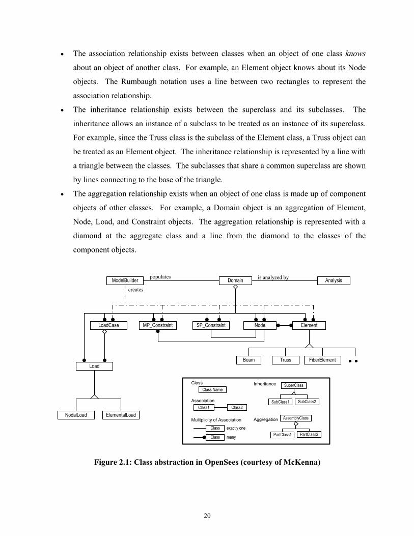
oriented FEA programs, the main class abstractions adopted in OpenSees to describe a finite
element model are: Node, Element, Constrain, Load, and Domain, etc. Figure 2.1 depicts the
main class abstractions in OpenSees and the relationship between the classes using the
Rumbaugh (Rumbaugh et al. 1991) notation. Details on each class and its interface can be found
in McKenna (McKenna 1997). The Rumbaugh notation uses a rectangle to represent a class, and
a line connecting two classes to represent the relationship between the two classes. There are
three types of relationships:
20
• The association relationship exists between classes when an object of one class knows
about an object of another class. For example, an Element object knows about its Node
objects. The Rumbaugh notation uses a line between two rectangles to represent the
association relationship.
• The inheritance relationship exists between the superclass and its subclasses. The
inheritance allows an instance of a subclass to be treated as an instance of its superclass.
For example, since the Truss class is the subclass of the Element class, a Truss object can
be treated as an Element object. The inheritance relationship is represented by a line with
a triangle between the classes. The subclasses that share a common superclass are shown
by lines connecting to the base of the triangle.
• The aggregation relationship exists when an object of one class is made up of component
objects of other classes. For example, a Domain object is an aggregation of Element,
Node, Load, and Constraint objects. The aggregation relationship is represented with a
diamond at the aggregate class and a line from the diamond to the classes of the
component objects.
Domain AnalysisModelBuilder
Node ElementSP_ConstraintMP_ConstraintLoadCase
LoadTruss FiberElementBeam
creates
populates is analyzed by
ElementalLoadNodalLoad
Class Name
Class2Class1
Class
Class exactly one
many
Class
Association
Mulitplicity of Association
SuperClass
SubClass2SubClass1
Inheritance
Aggregation AssemblyClass
PartClass2PartClass1
Figure 2.1: Class abstraction in OpenSees (courtesy of McKenna)
21
As shown in Figure 2.1, the ModelBuilder class defined in OpenSees is responsible for
creating finite element models, i.e., creating the nodes, elements, loads, and constraints. The
ModelBuilder class defines one pure virtual method, buildFE_Model(), which can be
invoked to create a finite element model. Subclasses of ModelBuilder must provide an
implementation of the method so that different types of finite element models can be created.
The usage of the ModelBuilder class hierarchy keeps OpenSees extendible. Each ModelBuilder
object, as shown in Figure 2.1, is associated with a single Domain object, which acts as a
repository for domain components. When buildFE_Model() is invoked on a ModelBuilder
object, the object builds the components of the model and then adds the component objects to the
Domain object. The manner in which the ModelBuilder object creates the model components
depends on the subclass of the ModelBuildler that is chosen to perform the analysis. This
approach allows an appropriate subclass of ModelBuilder to be used for creating certain type of
finite element models.
In OpenSees, a Domain object is associated with a ModelBuilder object and an Analysis
object, as shown in Figure 2.1. The ModelBuilder object is responsible for populating the
Domain object by creating the model component objects and then adding them to the Domain
object. The Analysis object is responsible for analyzing the populated Domain object.
The basic functionality of an Element object is to provide the current stiffness, mass, and
damping matrices, and the residual force vector due to the current stresses and element loads.
The Element class defined in OpenSees is an abstract base class, which defines the interface that
all subclasses must provide. Normally a new type of element can be introduced by simply
implementing a new Element subclass, which is usually a process that incurs no changes to the
existing code in the program. It should be noted that most finite element analysis programs
written in procedural languages also provide facilities for adding elements. However, the object-
oriented approach can better isolate the element functions from analysis and solution algorithm
functions. The object-oriented approach allows inheritance of common functions, and allows the
Element objects to store as much private data as required by the element. It is this level of
abstraction that facilitates the concurrent development of new elements and makes the
development of distributed element services easier.
For a finite element program, the ability to choose the type of analysis performed on the
analysis model is as important as changing element types. The typical object-oriented approach
that has been taken to the Analysis class design (Archer 1996; Dubois-Pelerin and Zimmermann
22
1993; Forde et al. 1990; Pidaparti and Hudli 1993; Zimmermann et al. 1992) is similar to the
black-box approach of traditional finite element programming. With this approach, a number of
subclasses of Analysis are provided, and each of these Analysis subclasses is associated with one
type of analysis (e.g., linear, transient, etc.). The hierarchy representing the Analysis classes is
very flat, which is not efficient to facilitate code reuse. To provide a design that is more flexible
and extendible than the typical approach, the main tasks performed in a finite element analysis
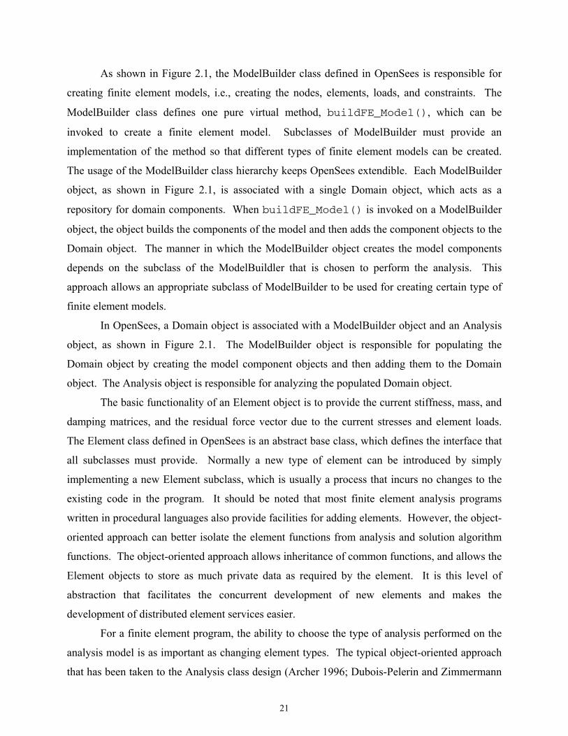
need to be identified, and separate classes can be abstracted for these tasks. The class diagram of
OpenSees analysis framework is shown in Figure 2.2. As depicted in the figure, OpenSees uses
an aggregation of classes to represent Analysis, which includes SolutionAlgorithm,
AnalysisModel, Integrator, ConstraintHandler, DOF_Numberer and SystemOfEqn.
AnalysisDomain
EigenAnalysisTransientAnalysisStaticAnalysis
SolverSystemOfEqn
SolutionAlgorithm IntegratorAnalysisModel ConstraintHandler DOF_Numberer
FE_ElementDOF_GroupNode Element
GraphNumberer
RCM
Figure 2.2: Class diagram for OpenSees analysis framework (courtesy of McKenna)
2.2 DIRECT MODULE INTEGRATION
As technologies and structural theories advance, finite element analysis software packages need
to be able to accommodate new developments in element formulation, material relations,
analysis strategies, solution strategies, as well as computing environments. For most existing
finite element software packages, modifying or extending the code requires that the developers
have intimate knowledge of the data structures and what procedures affect what portions of the
code. The ability to reuse code from other sources is limited, because data structures vary widely
between programs. Consequently, introducing code from other sources often requires that the
23
code be modified to suit the data structure used in the finite element program. The modification
of one portion of the program may also have a ripple effect that results in dramatic code changes
in other parts of the program.
To support better data encapsulation and to facilitate code reuse, the object-oriented
programming paradigm can be utilized for the finite element program development. A key
feature of object-oriented FEA programs is the interchangeability of components and the ability
to integrate existing libraries and new components into the framework without the need to
change the existing code. The flexibility and extendibility of these programs are based on the
object-oriented support of abstraction, encapsulation, inheritance, and polymorphism. Extending
existing programs by incorporating external modules normally requires one or several subclasses
to be introduced.
In the following, a number of examples of module extension are presented. Several
approaches for incorporating different types of software components are discussed. To illustrate
the principles and ideas without losing generality, we employ OpenSees as the core platform.
Similar techniques can be applied to other object-oriented FEA programs for integrating external
software modules.
2.2.1 Incorporating New Developments
One of the benefits of object-oriented software design is that new developed code can be
incorporated as one or several new classes. Because of the encapsulation and inheritance
features of object-oriented design, the integration process tends to be modular and incurs no
modifications to the existing code. For an object-oriented FEA program, the ease of
incorporating new developments and existing libraries also holds. Since the base classes for a
typical object-oriented FEA program are already defined, new elements, new material types, new
analysis strategies, and new solution strategies can be introduced by creating new subclasses of
the defined classes. This process can be exemplified with the modular integration of a new
element. In this section, we describe the process of modular extension of an object-oriented FEA
program through introducing subclasses, using the integration of an eight-node quadrilateral
element as an example.
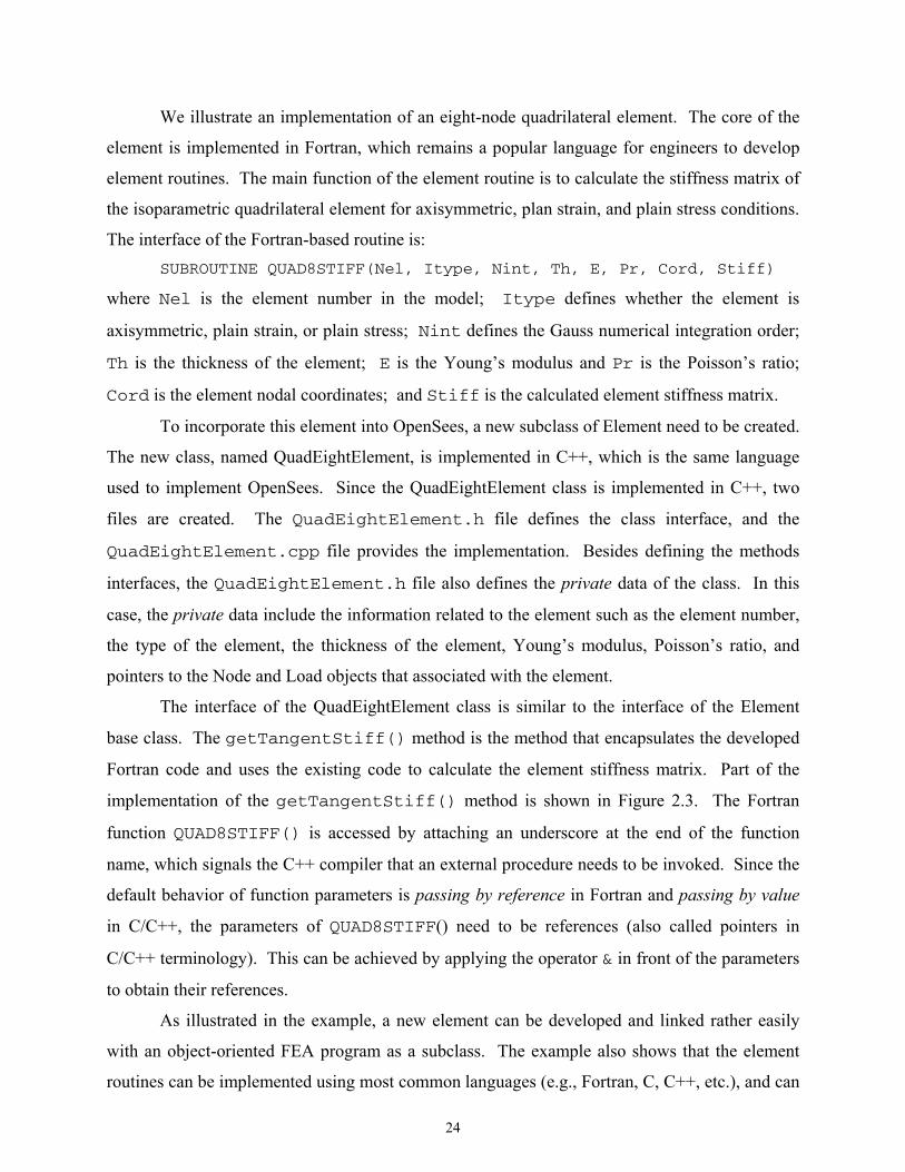
24
We illustrate an implementation of an eight-node quadrilateral element. The core of the
element is implemented in Fortran, which remains a popular language for engineers to develop
element routines. The main function of the element routine is to calculate the stiffness matrix of
the isoparametric quadrilateral element for axisymmetric, plan strain, and plain stress conditions.
The interface of the Fortran-based routine is: SUBROUTINE QUAD8STIFF(Nel, Itype, Nint, Th, E, Pr, Cord, Stiff)
where Nel is the element number in the model; Itype defines whether the element is
axisymmetric, plain strain, or plain stress; Nint defines the Gauss numerical integration order;
Th is the thickness of the element; E is the Young’s modulus and Pr is the Poisson’s ratio;
Cord is the element nodal coordinates; and Stiff is the calculated element stiffness matrix.
To incorporate this element into OpenSees, a new subclass of Element need to be created.
The new class, named QuadEightElement, is implemented in C++, which is the same language
used to implement OpenSees. Since the QuadEightElement class is implemented in C++, two
files are created. The QuadEightElement.h file defines the class interface, and the
QuadEightElement.cpp file provides the implementation. Besides defining the methods
interfaces, the QuadEightElement.h file also defines the private data of the class. In this
case, the private data include the information related to the element such as the element number,
the type of the element, the thickness of the element, Young’s modulus, Poisson’s ratio, and
pointers to the Node and Load objects that associated with the element.
The interface of the QuadEightElement class is similar to the interface of the Element
base class. The getTangentStiff() method is the method that encapsulates the developed
Fortran code and uses the existing code to calculate the element stiffness matrix. Part of the
implementation of the getTangentStiff() method is shown in Figure 2.3. The Fortran
function QUAD8STIFF() is accessed by attaching an underscore at the end of the function
name, which signals the C++ compiler that an external procedure needs to be invoked. Since the
default behavior of function parameters is passing by reference in Fortran and passing by value
in C/C++, the parameters of QUAD8STIFF() need to be references (also called pointers in
C/C++ terminology). This can be achieved by applying the operator & in front of the parameters
to obtain their references.
As illustrated in the example, a new element can be developed and linked rather easily
with an object-oriented FEA program as a subclass. The example also shows that the element
routines can be implemented using most common languages (e.g., Fortran, C, C++, etc.), and can
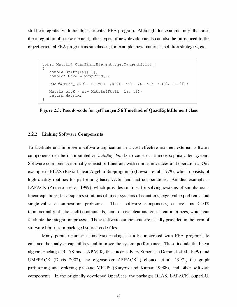
25
still be integrated with the object-oriented FEA program. Although this example only illustrates
the integration of a new element, other types of new developments can also be introduced to the
object-oriented FEA program as subclasses; for example, new materials, solution strategies, etc.
const Matrix& QuadEightElement::getTangentStiff() { double Stiff[16][16]; double* Cord = wrapCord(); QUAD8STIFF_(&Nel, &Itype, &Nint, &Th, &E, &Pr, Cord, Stiff); Matrix eleK = new Matrix(Stiff, 16, 16); return Matrix; }
Figure 2.3: Pseudo-code for getTangentStiff method of QuadEightElement class
2.2.2 Linking Software Components
To facilitate and improve a software application in a cost-effective manner, external software
components can be incorporated as building blocks to construct a more sophisticated system.
Software components normally consist of functions with similar interfaces and operations. One
example is BLAS (Basic Linear Algebra Subprograms) (Lawson et al. 1979), which consists of
high quality routines for performing basic vector and matrix operations. Another example is
LAPACK (Anderson et al. 1999), which provides routines for solving systems of simultaneous
linear equations, least-squares solutions of linear systems of equations, eigenvalue problems, and
single-value decomposition problems. These software components, as well as COTS
(commercially off-the-shelf) components, tend to have clear and consistent interfaces, which can
facilitate the integration process. These software components are usually provided in the form of
software libraries or packaged source-code files.
Many popular numerical analysis packages can be integrated with FEA programs to
enhance the analysis capabilities and improve the system performance. These include the linear
algebra packages BLAS and LAPACK, the linear solvers SuperLU (Demmel et al. 1999) and
UMFPACK (Davis 2002), the eigensolver ARPACK (Lehoucq et al. 1997), the graph
partitioning and ordering package METIS (Karypis and Kumar 1998b), and other software
components. In the originally developed OpenSees, the packages BLAS, LAPACK, SuperLU,
26
and UMFPACK have already been incorporated (McKenna 1997). In the following, we use the
integration of METIS version 4.0 with OpenSees to illustrate the process of incorporating off-
the-shelf software components.
METIS is a software package for partitioning large irregular graphs, partitioning large
meshes, and computing fill-reducing ordering of sparse matrices (Karypis and Kumar 1998b).
The algorithms in METIS are based on multilevel graph partitioning (Karypis and Kumar 1998a;
Karypis and Kumar 1998c). METIS provides both stand-alone programs (executable files) and
library interfaces (functions). To keep the integration flexible, we choose to use the library
interfaces. We are particularly interested in the usages of two METIS functions:
• METIS_PartGraphVKway(), which is used to partition a graph into k equal-size
parts using the multilevel k-way partitioning algorithm. The objective of the partitioning
is to minimize the total communication volume. This routine can be used for domain
decomposition, which is an important step for parallel finite element analysis.
• METIS_NodeND(), which is a function to compute fill-reducing orderings of sparse
matrices using the multilevel nested dissection algorithm. The nested dissection
paradigm is based on computing a vertex-seperator for the graph corresponding to the
matrix. The nodes in the separator are moved to the end of the matrix, and a similar
process is applied recursively for each one of the other two parts. This routine is very
useful for generating the ordering for sparse linear solver so that the storage of the sparse
matrix can be reduced.
The details of these two functions and their interfaces can be found in the METIS manual
(Karypis and Kumar 1998b). Both functions have input parameters xadj and adjncy, which
are two arrays used to represent the adjacency structure of a graph.
2.2.2.1 Graph Representation of Matrices
Graph theory plays a significant role in the study of sparse matrices (George and Liu 1981). A
graph G = (X, E) consists of a finite set of nodes or vertices together with a set of edges, which
are unordered pairs of vertices. The structure of a matrix can be symbolically represented as a
graph, where the row (or column) number of the matrix represents the vertices and the non-zero
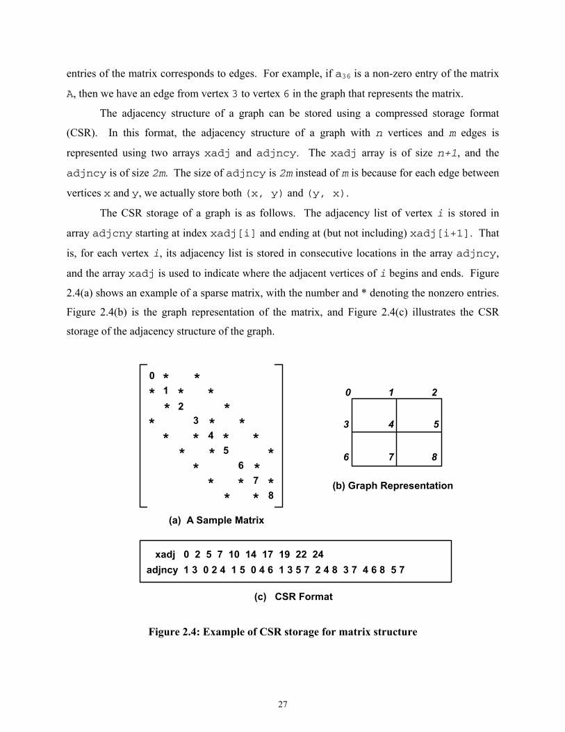
27
entries of the matrix corresponds to edges. For example, if a36 is a non-zero entry of the matrix
A, then we have an edge from vertex 3 to vertex 6 in the graph that represents the matrix.
The adjacency structure of a graph can be stored using a compressed storage format
(CSR). In this format, the adjacency structure of a graph with n vertices and m edges is
represented using two arrays xadj and adjncy. The xadj array is of size n+1, and the
adjncy is of size 2m. The size of adjncy is 2m instead of m is because for each edge between
vertices x and y, we actually store both (x, y) and (y, x).
The CSR storage of a graph is as follows. The adjacency list of vertex i is stored in
array adjcny starting at index xadj[i] and ending at (but not including) xadj[i+1]. That
is, for each vertex i, its adjacency list is stored in consecutive locations in the array adjncy,
and the array xadj is used to indicate where the adjacent vertices of i begins and ends. Figure
2.4(a) shows an example of a sparse matrix, with the number and * denoting the nonzero entries.
Figure 2.4(b) is the graph representation of the matrix, and Figure 2.4(c) illustrates the CSR
storage of the adjacency structure of the graph.
(b) Graph Representation
(c) CSR Format
0
87
65
43
21**
*
*
*
*
*
*
*
*
*
*
*
*
*
*
*
*
*
*
*
**
*
xadj 0 2 5 7 10 14 17 19 22 24adjncy 1 3 0 2 4 1 5 0 4 6 1 3 5 7 2 4 8 3 7 4 6 8 5 7
210
7
543
6 8
(a) A Sample Matrix
Figure 2.4: Example of CSR storage for matrix structure
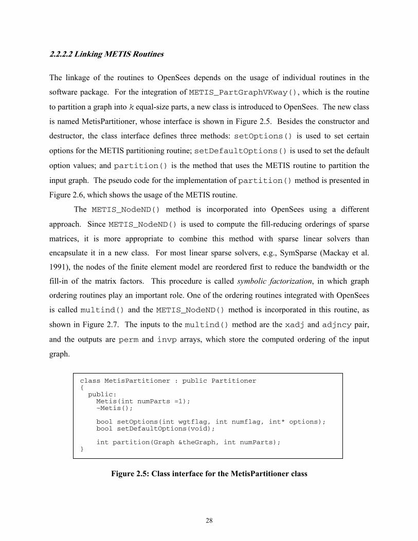
28
2.2.2.2 Linking METIS Routines
The linkage of the routines to OpenSees depends on the usage of individual routines in the
software package. For the integration of METIS_PartGraphVKway(), which is the routine
to partition a graph into k equal-size parts, a new class is introduced to OpenSees. The new class
is named MetisPartitioner, whose interface is shown in Figure 2.5. Besides the constructor and
destructor, the class interface defines three methods: setOptions() is used to set certain
options for the METIS partitioning routine; setDefaultOptions() is used to set the default
option values; and partition() is the method that uses the METIS routine to partition the
input graph. The pseudo code for the implementation of partition() method is presented in
Figure 2.6, which shows the usage of the METIS routine.
The METIS_NodeND() method is incorporated into OpenSees using a different
approach. Since METIS_NodeND() is used to compute the fill-reducing orderings of sparse
matrices, it is more appropriate to combine this method with sparse linear solvers than
encapsulate it in a new class. For most linear sparse solvers, e.g., SymSparse (Mackay et al.
1991), the nodes of the finite element model are reordered first to reduce the bandwidth or the
fill-in of the matrix factors. This procedure is called symbolic factorization, in which graph
ordering routines play an important role. One of the ordering routines integrated with OpenSees
is called multind() and the METIS_NodeND() method is incorporated in this routine, as
shown in Figure 2.7. The inputs to the multind() method are the xadj and adjncy pair,
and the outputs are perm and invp arrays, which store the computed ordering of the input
graph.
class MetisPartitioner : public Partitioner { public: Metis(int numParts =1); ~Metis(); bool setOptions(int wgtflag, int numflag, int* options); bool setDefaultOptions(void); int partition(Graph &theGraph, int numParts); }
Figure 2.5: Class interface for the MetisPartitioner class
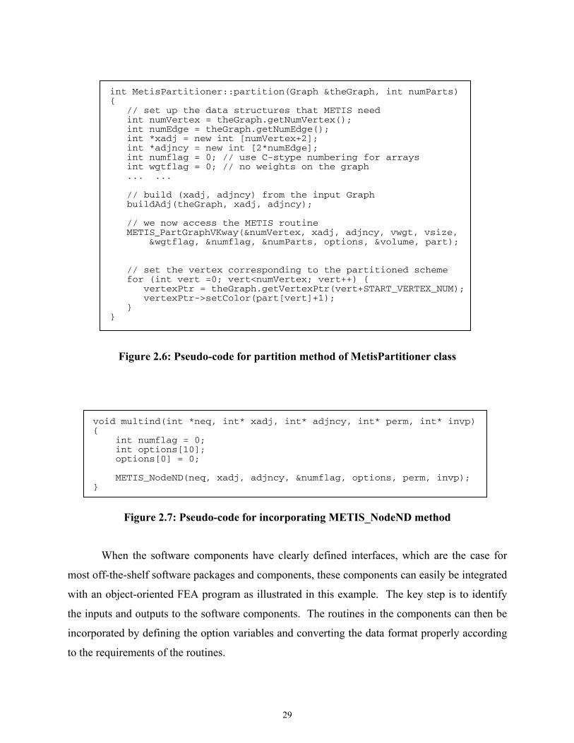
29
int MetisPartitioner::partition(Graph &theGraph, int numParts) { // set up the data structures that METIS need int numVertex = theGraph.getNumVertex(); int numEdge = theGraph.getNumEdge(); int *xadj = new int [numVertex+2]; int *adjncy = new int [2*numEdge]; int numflag = 0; // use C-stype numbering for arrays int wgtflag = 0; // no weights on the graph ... ... // build (xadj, adjncy) from the input Graph buildAdj(theGraph, xadj, adjncy); // we now access the METIS routine METIS_PartGraphVKway(&numVertex, xadj, adjncy, vwgt, vsize, &wgtflag, &numflag, &numParts, options, &volume, part); // set the vertex corresponding to the partitioned scheme for (int vert =0; vert<numVertex; vert++) { vertexPtr = theGraph.getVertexPtr(vert+START_VERTEX_NUM); vertexPtr->setColor(part[vert]+1); } }
Figure 2.6: Pseudo-code for partition method of MetisPartitioner class
void multind(int *neq, int* xadj, int* adjncy, int* perm, int* invp) { int numflag = 0; int options[10]; options[0] = 0; METIS_NodeND(neq, xadj, adjncy, &numflag, options, perm, invp); }
Figure 2.7: Pseudo-code for incorporating METIS_NodeND method
When the software components have clearly defined interfaces, which are the case for
most off-the-shelf software packages and components, these components can easily be integrated
with an object-oriented FEA program as illustrated in this example. The key step is to identify
the inputs and outputs to the software components. The routines in the components can then be
incorporated by defining the option variables and converting the data format properly according
to the requirements of the routines.
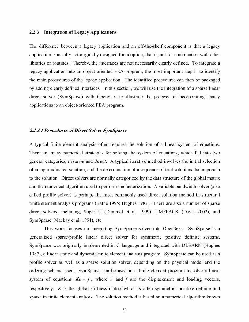
30
2.2.3 Integration of Legacy Applications
The difference between a legacy application and an off-the-shelf component is that a legacy
application is usually not originally designed for adoption, that is, not for combination with other
libraries or routines. Thereby, the interfaces are not necessarily clearly defined. To integrate a
legacy application into an object-oriented FEA program, the most important step is to identify
the main procedures of the legacy application. The identified procedures can then be packaged
by adding clearly defined interfaces. In this section, we will use the integration of a sparse linear
direct solver (SymSparse) with OpenSees to illustrate the process of incorporating legacy
applications to an object-oriented FEA program.
2.2.3.1 Procedures of Direct Solver SymSparse
A typical finite element analysis often requires the solution of a linear system of equations.
There are many numerical strategies for solving the system of equations, which fall into two
general categories, iterative and direct. A typical iterative method involves the initial selection
of an approximated solution, and the determination of a sequence of trial solutions that approach
to the solution. Direct solvers are normally categorized by the data structure of the global matrix
and the numerical algorithm used to perform the factorization. A variable bandwidth solver (also
called profile solver) is perhaps the most commonly used direct solution method in structural
finite element analysis programs (Bathe 1995; Hughes 1987). There are also a number of sparse
direct solvers, including, SuperLU (Demmel et al. 1999), UMFPACK (Davis 2002), and
SymSparse (Mackay et al. 1991), etc.
This work focuses on integrating SymSparse solver into OpenSees. SymSparse is a
generalized sparse/profile linear direct solver for symmetric positive definite systems.
SymSparse was originally implemented in C language and integrated with DLEARN (Hughes
1987), a linear static and dynamic finite element analysis program. SymSparse can be used as a
profile solver as well as a sparse solution solver, depending on the physical model and the
ordering scheme used. SymSparse can be used in a finite element program to solve a linear
system of equations fKu = , where u and f are the displacement and loading vectors,
respectively. K is the global stiffness matrix which is often symmetric, positive definite and
sparse in finite element analysis. The solution method is based on a numerical algorithm known
31
as Cholesky’s method, which is a symmetric variant of Gaussian elimination tailored to
symmetric positive definite matrices. During the solution process, the symmetric matrix A is
first factored into its matrix product, TLDLK = , where D is a diagonal matrix and L is the lower
triangular matrix factor. The displacement vector u is then computed by a forward solve,
fDLz T 1)( −= , followed by a backward substitution, zLu 1−= .
One important fact about the Cholesky factorization of a sparse matrix is that the matrix
usually suffers fill-in. That is, the matrix factor L has nonzeros in positions which are zero in the
lower triangular part of the matrix K. Therefore, in order to save storage requirement, the data
structure needs to be set up for the matrix factor L before the numerical calculation; and the same
data structure can be used to store the lower triangular part of matrix K. The SymSparse solver
includes a symbolic factorization procedure that determines and sets up the data structure for the
sparse matrix factor L directly. Dynamic memory allocation is used extensively in SymSparse to
set up the data structure. This one-step approach to establish the data structure for the matrix
factor is generally more efficient than the two-step approach adopted in (Liu 1991), which uses
symbolic factorization to determine the structure of the Cholesky factor first and then set up the
data structure based on the Cholesky structure.
Since SymSparse was originally developed to use with DLEARN (Hughes 1987), a
procedural finite element analysis program, we first need to identify the major procedures in
SymSparse in order to integrate it with an object-oriented FEA program. There are three main
tasks identified for the SymSparse solver, and these three main procedures are packaged with
clearly defined interfaces. For the interfaces shown in the following functions, the matrix factor
L and its data structure Ls are defined for illustration purposes only. The details regarding the
data structure are presented in Mackay et al. (Mackay et al. 1991).
• symbolicFact(neq, xadj, adjncy, invp, Ls)
Given the number of equations (neq) and the adjacency structure (xadj, adjncy) of a
matrix, this symbolic factorization routine determines the matrix ordering invp and a
data structure for the matrix factor, indicated as Ls. The input graph is first ordered by a
graph fill-reducing ordering routine. Currently, the ordering routines included are RCM
(George 1971), Minimum Degree (Tinney and Walker 1967), Generalized Nested
Dissection (Lipton et al. 1979), and Multilevel Nested Dissection (Karypis and Kumar
1998a). After the ordering, an ordered elimination tree can be established, and then a
topological postordering strategy is used to re-order the nodes so that the nodes in any
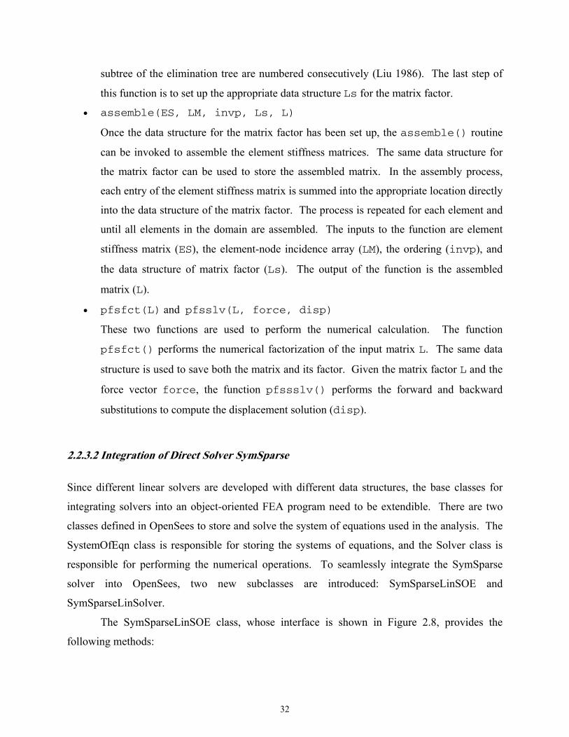
32
subtree of the elimination tree are numbered consecutively (Liu 1986). The last step of
this function is to set up the appropriate data structure Ls for the matrix factor.
• assemble(ES, LM, invp, Ls, L)
Once the data structure for the matrix factor has been set up, the assemble() routine
can be invoked to assemble the element stiffness matrices. The same data structure for
the matrix factor can be used to store the assembled matrix. In the assembly process,
each entry of the element stiffness matrix is summed into the appropriate location directly
into the data structure of the matrix factor. The process is repeated for each element and
until all elements in the domain are assembled. The inputs to the function are element
stiffness matrix (ES), the element-node incidence array (LM), the ordering (invp), and
the data structure of matrix factor (Ls). The output of the function is the assembled
matrix (L).
• pfsfct(L) and pfsslv(L, force, disp)
These two functions are used to perform the numerical calculation. The function
pfsfct() performs the numerical factorization of the input matrix L. The same data
structure is used to save both the matrix and its factor. Given the matrix factor L and the
force vector force, the function pfssslv() performs the forward and backward
substitutions to compute the displacement solution (disp).
2.2.3.2 Integration of Direct Solver SymSparse
Since different linear solvers are developed with different data structures, the base classes for
integrating solvers into an object-oriented FEA program need to be extendible. There are two
classes defined in OpenSees to store and solve the system of equations used in the analysis. The
SystemOfEqn class is responsible for storing the systems of equations, and the Solver class is
responsible for performing the numerical operations. To seamlessly integrate the SymSparse
solver into OpenSees, two new subclasses are introduced: SymSparseLinSOE and
SymSparseLinSolver.
The SymSparseLinSOE class, whose interface is shown in Figure 2.8, provides the
following methods:
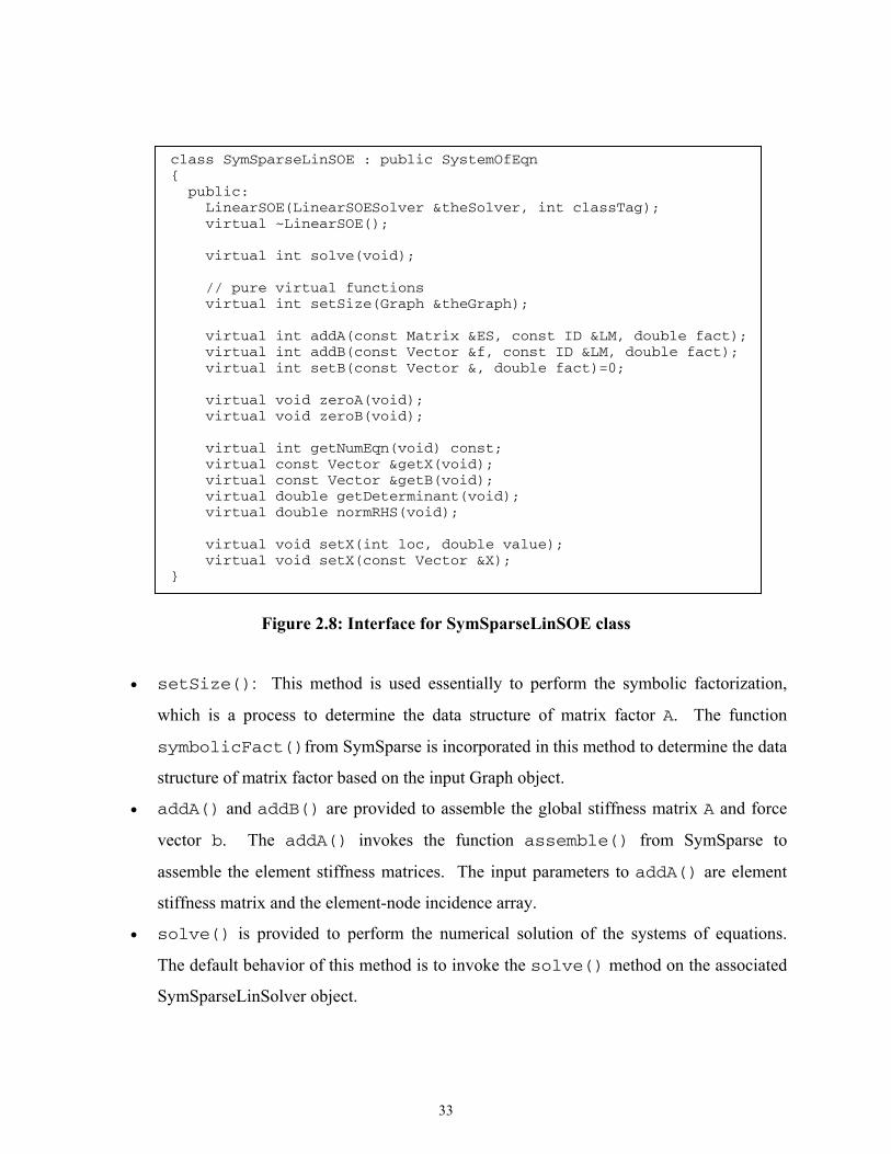
33
class SymSparseLinSOE : public SystemOfEqn { public: LinearSOE(LinearSOESolver &theSolver, int classTag); virtual ~LinearSOE(); virtual int solve(void); // pure virtual functions virtual int setSize(Graph &theGraph); virtual int addA(const Matrix &ES, const ID &LM, double fact); virtual int addB(const Vector &f, const ID &LM, double fact); virtual int setB(const Vector &, double fact)=0; virtual void zeroA(void); virtual void zeroB(void); virtual int getNumEqn(void) const; virtual const Vector &getX(void); virtual const Vector &getB(void); virtual double getDeterminant(void); virtual double normRHS(void); virtual void setX(int loc, double value); virtual void setX(const Vector &X); }
Figure 2.8: Interface for SymSparseLinSOE class
• setSize(): This method is used essentially to perform the symbolic factorization,
which is a process to determine the data structure of matrix factor A. The function
symbolicFact()from SymSparse is incorporated in this method to determine the data
structure of matrix factor based on the input Graph object.
• addA() and addB() are provided to assemble the global stiffness matrix A and force
vector b. The addA() invokes the function assemble() from SymSparse to
assemble the element stiffness matrices. The input parameters to addA() are element
stiffness matrix and the element-node incidence array.
• solve() is provided to perform the numerical solution of the systems of equations.
The default behavior of this method is to invoke the solve() method on the associated
SymSparseLinSolver object.
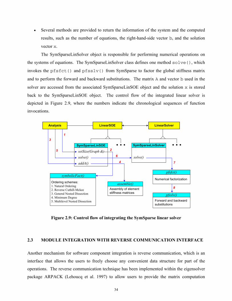
34
• Several methods are provided to return the information of the system and the computed
results, such as the number of equations, the right-hand-side vector b, and the solution
vector x.
The SymSparseLinSolver object is responsible for performing numerical operations on
the systems of equations. The SymSparseLinSolver class defines one method solve(), which
invokes the pfsfct() and pfsslv() from SymSparse to factor the global stiffness matrix
and to perform the forward and backward substitutions. The matrix A and vector b used in the
solver are accessed from the associated SymSparseLinSOE object and the solution x is stored
back to the SymSparseLinSOE object. The control flow of the integrated linear solver is
depicted in Figure 2.9, where the numbers indicate the chronological sequences of function
invocations.
Analysis
3
SymSparseLinSOE SymSparseLinSolver
setSize(Graph &) solve() addA()
solve()
1
symbolicFact()
Ordering schemes:1. Natural Ordering2. Reverse Cuthill-Mckee3. General Nested Dissection4. Minimum Degree5. Multilevel Nested Dissection
pfsfct()
Numerical factorization
2
4
5
LinearSOE LinearSolver
pfsslv() Forward and backward substitutions
6
assemble() Assembly of element stiffness matrices
8
7
Figure 2.9: Control flow of integrating the SymSparse linear solver
2.3 MODULE INTEGRATION WITH REVERSE COMMUNICATION INTERFACE
Another mechanism for software component integration is reverse communication, which is an
interface that allows the users to freely choose any convenient data structure for part of the
operations. The reverse communication technique has been implemented within the eigensolver
package ARPACK (Lehoucq et al. 1997) to allow users to provide the matrix computation
35
through subroutine calls or code segments. An object-oriented FEA program can also take
advantage of such mechanism to integrate software components. This section shows the
example of extending the OpenSees core for eigenvalue analysis, and the examples of
incorporating eigensolvers through reverse communication interface.
2.3.1 Reverse Communication Interface
For certain special function libraries and linear algebra libraries for dense matrices (e.g., BLAS
(Lawson et al. 1979) and LAPACK (Anderson et al. 1999)), the data structures are simple and
natural for the applications. However, this is hardly the case for the modern generation of
sophisticated numerical applications, where the problem is large and complex, and a significant
amount of design and coding are related to data structures. For instance, there are a large
number of different data structures developed for sparse matrices, which makes it difficult to
develop a numerical application that accommodates all possible cases. One obvious solution
would be to limit the number of possible data storage schemes and to transform the data
structures to a few possible supported choices, using transformation routines from libraries such
as SPARSKIT (Saad 1990). However, limiting the number of possible data storage schemes is
not convenient for the user, and may incur performance penalties because the data transformation
can be expensive to perform.
Another approach to handle the diverse application data structures is by using a reverse
communication interface as implemented in ARPACK (Lehoucq et al. 1997). In this approach,
routines that need to use the application data structures set a flag and return to the users. For the
applications involved with sparse matrices, reverse communication means that a data storage
scheme is not enforced on the matrices. The matrix itself is not needed in the main drive of the
application, but rather the matrix operations are required to be provided by the users.
The reverse communication mechanism can be applied to many types of applications; one
of such is the eigensolver. A typical generalized eigensolver requires vector-only operations and
matrix-dependent operations, such as matrix-vector multiplication xM ⋅ and the solution of
linear equations bxA =⋅ . Since the vectors are usually stored as contiguous arrays of bytes, the
vector-only operations are implemented within the eigensolver. The matrix-dependent
operations, on the other hand, are handled in a user-defined way. The main loop of the
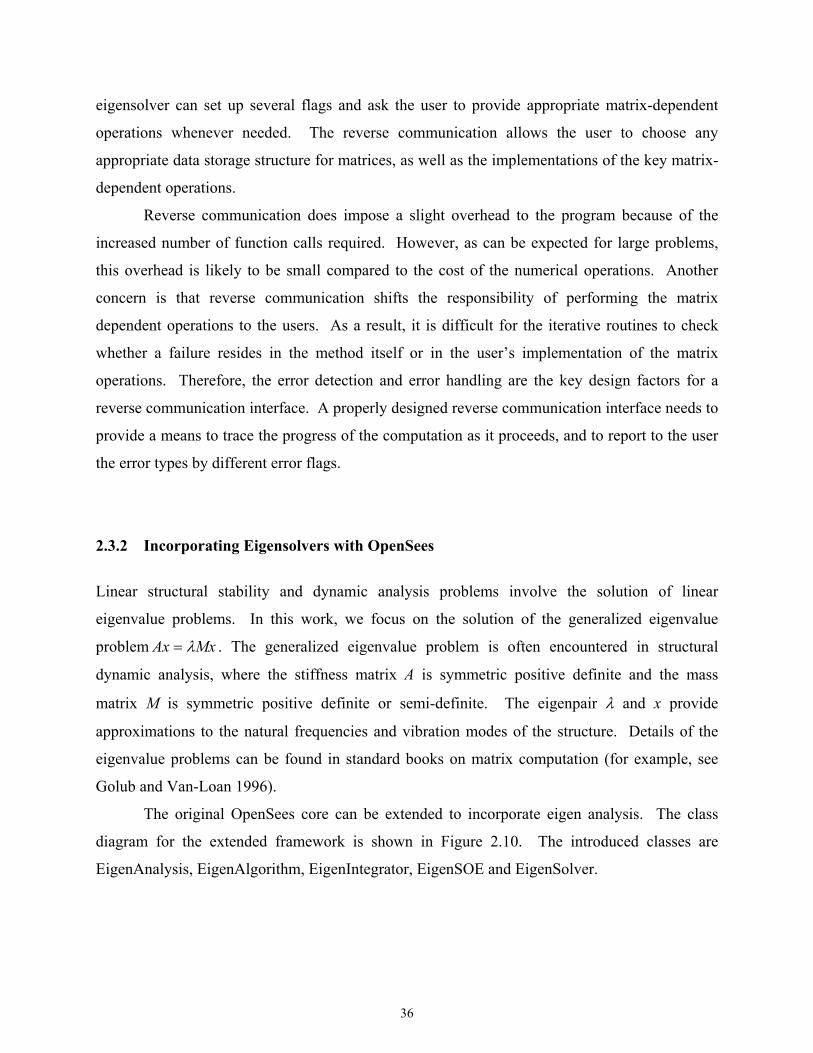
36
eigensolver can set up several flags and ask the user to provide appropriate matrix-dependent
operations whenever needed. The reverse communication allows the user to choose any
appropriate data storage structure for matrices, as well as the implementations of the key matrix-
dependent operations.
Reverse communication does impose a slight overhead to the program because of the
increased number of function calls required. However, as can be expected for large problems,
this overhead is likely to be small compared to the cost of the numerical operations. Another
concern is that reverse communication shifts the responsibility of performing the matrix
dependent operations to the users. As a result, it is difficult for the iterative routines to check
whether a failure resides in the method itself or in the user’s implementation of the matrix
operations. Therefore, the error detection and error handling are the key design factors for a
reverse communication interface. A properly designed reverse communication interface needs to
provide a means to trace the progress of the computation as it proceeds, and to report to the user
the error types by different error flags.
2.3.2 Incorporating Eigensolvers with OpenSees
Linear structural stability and dynamic analysis problems involve the solution of linear
eigenvalue problems. In this work, we focus on the solution of the generalized eigenvalue
problem MxAx λ= . The generalized eigenvalue problem is often encountered in structural
dynamic analysis, where the stiffness matrix A is symmetric positive definite and the mass
matrix M is symmetric positive definite or semi-definite. The eigenpair λ and x provide
approximations to the natural frequencies and vibration modes of the structure. Details of the
eigenvalue problems can be found in standard books on matrix computation (for example, see
Golub and Van-Loan 1996).
The original OpenSees core can be extended to incorporate eigen analysis. The class
diagram for the extended framework is shown in Figure 2.10. The introduced classes are
EigenAnalysis, EigenAlgorithm, EigenIntegrator, EigenSOE and EigenSolver.
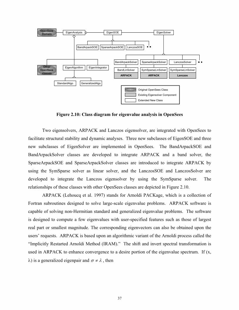
37
EigenAnalysis EigenSOE EigenSolver
BandArpackSOE SparseArpackSOE
BandArpackSolver SparseArpackSolver
BandLinSolver SymSparseLinSolverEigenIntegrator
OpenSeesDomain
ARPACK ARPACK
EigenAlgorithmOtherOpenSees
classes
GeneralizedAlgoStandardAlgo
LanczosSOE
LanczosSolver
SymSparseLinSolver
Lanczos
Original OpenSees Class
Existing Eigensolver Component
Extended New Class
Figure 2.10: Class diagram for eigenvalue analysis in OpenSees
Two eigensolvers, ARPACK and Lanczos eigensolver, are integrated with OpenSees to
facilitate structural stability and dynamic analyses. Three new subclasses of EigenSOE and three
new subclasses of EigenSolver are implemented in OpenSees. The BandArpackSOE and
BandArpackSolver classes are developed to integrate ARPACK and a band solver, the
SparseArpackSOE and SparseArpackSolver classes are introduced to integrate ARPACK by
using the SymSparse solver as linear solver, and the LanczosSOE and LanczosSolver are
developed to integrate the Lanczos eigensolver by using the SymSparse solver. The
relationships of these classes with other OpenSees classes are depicted in Figure 2.10.
ARPACK (Lehoucq et al. 1997) stands for Arnoldi PACKage, which is a collection of
Fortran subroutines designed to solve large-scale eigenvalue problems. ARPACK software is
capable of solving non-Hermitian standard and generalized eigenvalue problems. The software
is designed to compute a few eigenvalues with user-specified features such as those of largest
real part or smallest magnitude. The corresponding eigenvectors can also be obtained upon the
users’ requests. ARPACK is based upon an algorithmic variant of the Arnoldi process called the
“Implicitly Restarted Arnoldi Method (IRAM).” The shift and invert spectral transformation is
used in ARPACK to enhance convergence to a desire portion of the eigenvalue spectrum. If (x,
λ) is a generalized eigenpair and λσ ≠ , then
38
νσ xMxMA =− −1)( where σλ
ν−
=1
This transformation is effective for finding eigenvalues near σ.
One of the salient features of ARPACK is the reverse communication, which allows the
user to provide matrix-dependent operations. In order to use ARPACK to solve generalized
eigenvalue problems, two operations need to be provided by the user: one is matrix-vector
multiplication Mxz ← , and the other is a linear equation solver yMAx 1)( −−← σ .
• If the operation of matrix-vector multiplication is performed in the global level, the
operation requires the assembly of element mass matrices, which is an expensive
operation in terms of both processing time and extra storage space. To improve
performance and minimize storage requirement, the operation Mxz ← can be performed
using an element-by-element strategy. The mass matrix stored in each element is
retrieved to multiply with part of the vector x. The generated result vector can then be
assembled to obtain z. Compared with global matrix (two-dimensional) assembly, this
global vector (one-dimensional) assembly is much cheaper.
• For the solution of linear equations yMAx 1)( −−← σ , an efficient linear solver can be
used. Since the matrix )( MA σ− generated from dynamic analyses is normally sparse,
symmetric and positive definite, the SymSparse solver can be integrated to provide the
linear equation solving operation.
We will use the SparseArpackSolver class to illustrate the usage of reverse
communication. Figure 2.11 shows part of the pseudo-code for the implementation of the
solve() method in the SparseArpackSolver class. The pfsfct() and pfsslv() functions
are provided by the SymSparse solver to solve linear equations, and the myMv() is a subroutine
performing matrix-vector multiplication. The dsaupd() and dseupd() are ARPACK
subroutines to compute approximations to a few eigenpairs. For the main loop shown in Figure
2.11, different matrix-dependent operation is taken with different flag (ido) value, which is a
control indicator generated by ARPARCK subroutine dsaupd(). By setting the value of this
flag, ARPACK tells the client code the required operation or the status of the analysis. After the
main loop returns and no fatal errors have occurred, the dseupd() is invoked to obtain the
eigenvalues and the corresponding eigenvectors if desired. The dseupd() method performs
39
eigenvector purification, which is a process to recover eigenvectors when the M matrix is ill-
conditioned.
Besides ARPACK routines, a Lanczos eigensolver is also integrated with OpenSees. The
implementation of the Lanczos eigensolver mainly follows the spectral transformation Lanczos
method developed by Ericsson and Ruhe (1980), the Lanczos vector reorthogonalization scheme
proposed by Grimes et al. (Grimes et al. 1994), and some refinements developed by Mackay et
al. (Mackay 1992). The linking with the Lanczos eigensolver takes the same strategy as
incorporating ARPACK. The solve() method of the LanczosSolver class uses a similar
reverse communication loop as the one shown in Figure 2.11.
// call a routine to factor the matrix (A-sigma*M). factor = pfsfct(n, diag, penv, nblks, xblk, begblk, first, rowblks); while (true) { // repeatedly call the routine DSAUPD from ARPACK and take // corresponding actions indicated by flag ido. dsaupd_(&ido, &bmat, &n, which, &nev, &tol, resid, &ncv, v, &ldv, iparam, ipntr, workd, workl, &lworkl, &info); if (ido == -1) { // perform y <-- M*x // perform y <-- inv[A-sigma*M]*M*x. // pfsslv() is a routine for solving linear equations. // x = workd[ipntr[0]-1] // y = workd[ipntr[1]-1] myMv(n, &workd[ipntr[0]-1], &workd[ipntr[1]-1]); pfsslv(n, diag, penv, nblks, xblk, &workd[ipntr[1]-1], begblk); continue; } else if (ido == 1) { // perform y <-- inv[A-sigma*M]*M*x // M*x = workd[ipntr[2]-1] // y = workd[ipntr[1]-1] myCopy(n, &workd[ipntr[2]-1], &workd[ipntr[1]-1]); pfsslv(n, diag, penv, nblks, xblk, &workd[ipntr[1]-1], begblk); continue; } else if (ido == 2) { // perform y <-- M*x // x = workd[ipntr[0]-1] // y = workd[ipntr[1]-1] myMv(n, &workd[ipntr[0]-1], &workd[ipntr[1]-1]); continue; } break; } // if no fatal errors occur, use DSEUPD for post processing // requested eigenvectors may be computed and extracted. dseupd_(&rvec, &howmy, select, d, v, &ldv, &sigma, &bmat, &n, which, &nev, &tol, resid, &ncv, v, &ldv, iparam, ipntr, workd, workl, &lworkl, &info);
Figure 2.11: Linking ARPACK through reverse communication interface
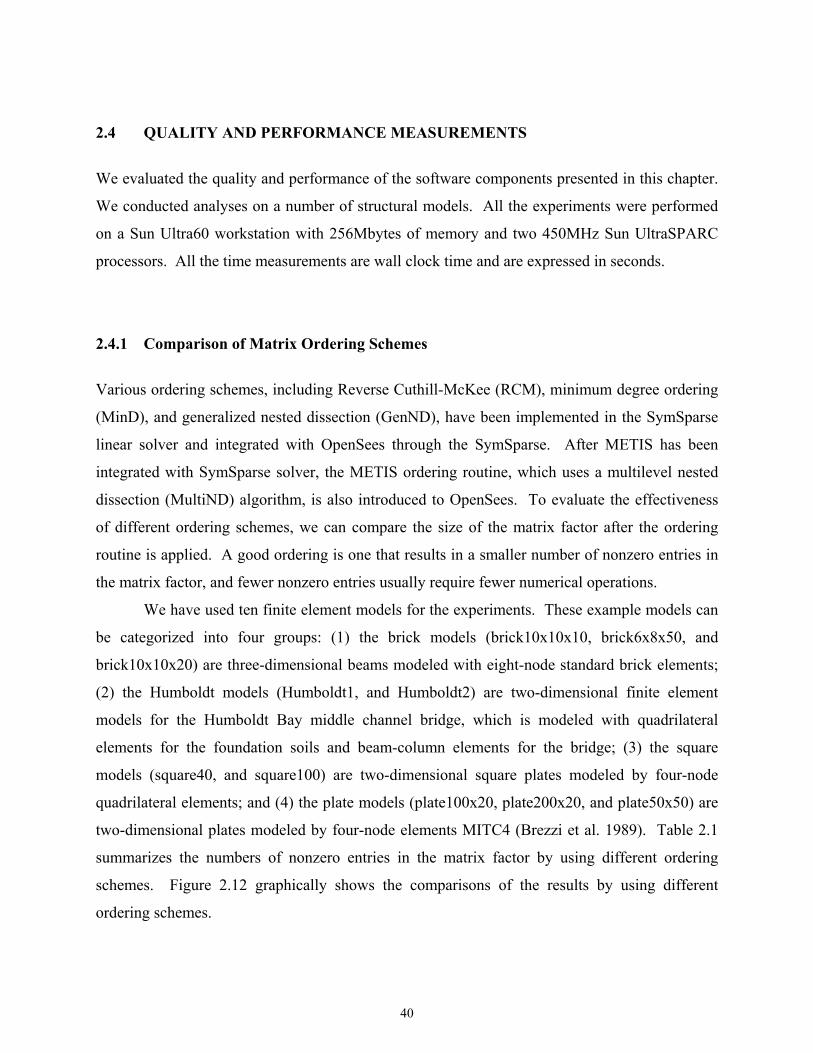
40
2.4 QUALITY AND PERFORMANCE MEASUREMENTS
We evaluated the quality and performance of the software components presented in this chapter.
We conducted analyses on a number of structural models. All the experiments were performed
on a Sun Ultra60 workstation with 256Mbytes of memory and two 450MHz Sun UltraSPARC
processors. All the time measurements are wall clock time and are expressed in seconds.
2.4.1 Comparison of Matrix Ordering Schemes
Various ordering schemes, including Reverse Cuthill-McKee (RCM), minimum degree ordering
(MinD), and generalized nested dissection (GenND), have been implemented in the SymSparse
linear solver and integrated with OpenSees through the SymSparse. After METIS has been
integrated with SymSparse solver, the METIS ordering routine, which uses a multilevel nested
dissection (MultiND) algorithm, is also introduced to OpenSees. To evaluate the effectiveness
of different ordering schemes, we can compare the size of the matrix factor after the ordering
routine is applied. A good ordering is one that results in a smaller number of nonzero entries in
the matrix factor, and fewer nonzero entries usually require fewer numerical operations.
We have used ten finite element models for the experiments. These example models can
be categorized into four groups: (1) the brick models (brick10x10x10, brick6x8x50, and
brick10x10x20) are three-dimensional beams modeled with eight-node standard brick elements;
(2) the Humboldt models (Humboldt1, and Humboldt2) are two-dimensional finite element
models for the Humboldt Bay middle channel bridge, which is modeled with quadrilateral
elements for the foundation soils and beam-column elements for the bridge; (3) the square
models (square40, and square100) are two-dimensional square plates modeled by four-node
quadrilateral elements; and (4) the plate models (plate100x20, plate200x20, and plate50x50) are
two-dimensional plates modeled by four-node elements MITC4 (Brezzi et al. 1989). Table 2.1
summarizes the numbers of nonzero entries in the matrix factor by using different ordering
schemes. Figure 2.12 graphically shows the comparisons of the results by using different
ordering schemes.
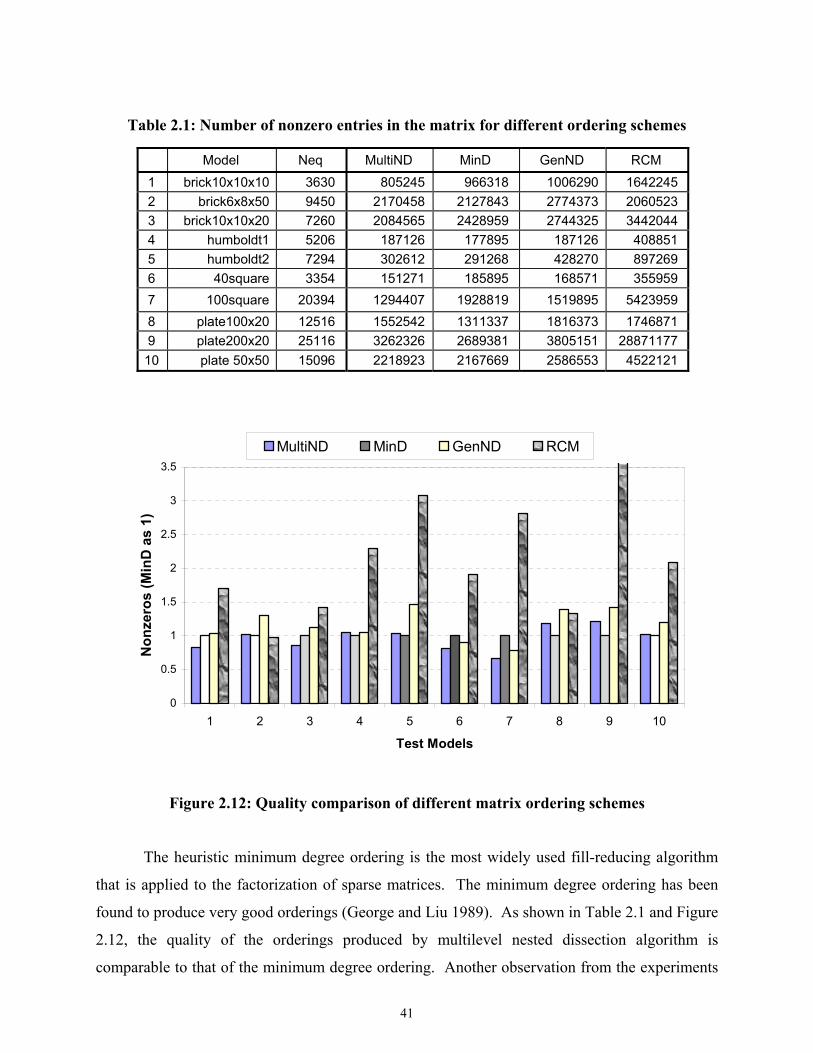
41
Table 2.1: Number of nonzero entries in the matrix for different ordering schemes
Model Neq MultiND MinD GenND RCM 1 brick10x10x10 3630 805245 966318 1006290 1642245 2 brick6x8x50 9450 2170458 2127843 2774373 2060523 3 brick10x10x20 7260 2084565 2428959 2744325 3442044 4 humboldt1 5206 187126 177895 187126 408851 5 humboldt2 7294 302612 291268 428270 897269 6 40square 3354 151271 185895 168571 355959 7 100square 20394 1294407 1928819 1519895 5423959 8 plate100x20 12516 1552542 1311337 1816373 1746871 9 plate200x20 25116 3262326 2689381 3805151 28871177 10 plate 50x50 15096 2218923 2167669 2586553 4522121
0
0.5
1
1.5
2
2.5
3
3.5
1 2 3 4 5 6 7 8 9 10
Test Models
Non
zero
s (M
inD
as
1)
MultiND MinD GenND RCM
Figure 2.12: Quality comparison of different matrix ordering schemes
The heuristic minimum degree ordering is the most widely used fill-reducing algorithm
that is applied to the factorization of sparse matrices. The minimum degree ordering has been
found to produce very good orderings (George and Liu 1989). As shown in Table 2.1 and Figure
2.12, the quality of the orderings produced by multilevel nested dissection algorithm is
comparable to that of the minimum degree ordering. Another observation from the experiments
42
is that the multilevel nested dissection algorithm generates better orderings than the generalized
nested dissection ordering. Since the reverse Cuthill-McKee ordering is used to generate
orderings for the profile storage of matrices, the number of nonzero entries is often substantially
larger than other ordering algorithms.
2.4.2 Performance Comparison of Linear Solvers
The same finite element models used for testing ordering schemes were also used for the
performance comparison of different linear solvers. We tested the following linear solvers:
SymSparse with multilevel nested dissection ordering (MultiND), SymSparse with minimum
degree ordering (MinD), SymSparse with generalized nested dissection ordering (GenND),
profile solver (Profile), SuperLU solver (SuperLU), and UMFPACK solver (UmfPack). The
solution time for various linear solvers is summarized in Table 2.2 and depicted in Figure 2.13.
The solution time is the wall clock time for performing symbolic factorization, numerical
factorization, and forward and backward substitutions. The time for assembling element
stiffness matrices is not included. The value NA in Table 2.2 indicates that the solution time is
substantially larger than when using other solvers. The long solution time is primarily due to the
large number of page faults. In a paged virtual memory operating system (e.g., Windows, Unix),
a page fault usually occurs when the physical memory is consumed. In this case, an access to a
page (block) of memory cannot be mapped to physical memory, thus the operating system has to
fetch the page into memory from secondary storage (usually disk). Since accessing disk is much
slower than accessing physical memory, page faults can substantially degrade the system
performance.
The experimental results clearly show that the performance of a linear solver is directly
related to the matrix storage requirement. The more nonzero entries in the matrix factor for a
linear solver, the more numerical operations are needed for factorization. In this sense, the
ordering algorithms and data structures are very important for sparse matrix computation and the
solution of linear systems, as they can minimize the matrix storage requirement and facilitate the
data element access.
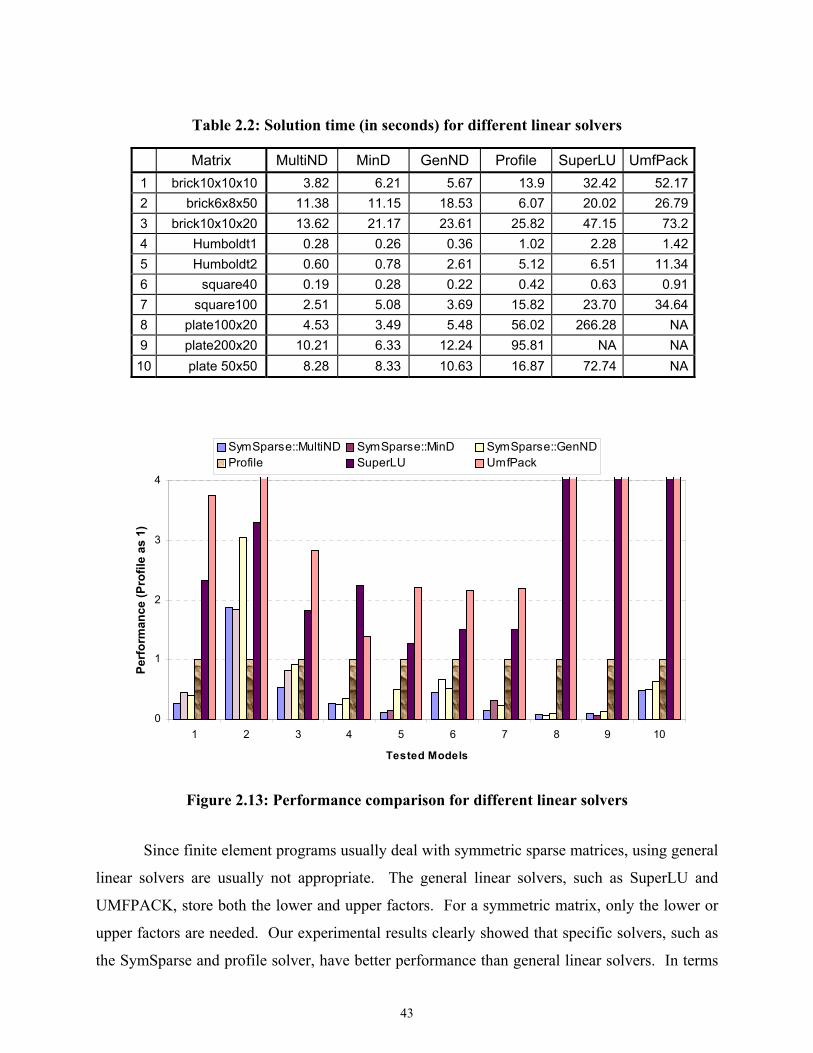
43
Table 2.2: Solution time (in seconds) for different linear solvers
Matrix MultiND MinD GenND Profile SuperLU UmfPack1 brick10x10x10 3.82 6.21 5.67 13.9 32.42 52.172 brick6x8x50 11.38 11.15 18.53 6.07 20.02 26.793 brick10x10x20 13.62 21.17 23.61 25.82 47.15 73.24 Humboldt1 0.28 0.26 0.36 1.02 2.28 1.425 Humboldt2 0.60 0.78 2.61 5.12 6.51 11.346 square40 0.19 0.28 0.22 0.42 0.63 0.917 square100 2.51 5.08 3.69 15.82 23.70 34.648 plate100x20 4.53 3.49 5.48 56.02 266.28 NA9 plate200x20 10.21 6.33 12.24 95.81 NA NA10 plate 50x50 8.28 8.33 10.63 16.87 72.74 NA
0
1
2
3
4
1 2 3 4 5 6 7 8 9 10
Tested Models
Perf
orm
ance
(Pro
file
as 1
)
SymSparse::MultiND SymSparse::MinD SymSparse::GenNDProfile SuperLU UmfPack
Figure 2.13: Performance comparison for different linear solvers
Since finite element programs usually deal with symmetric sparse matrices, using general
linear solvers are usually not appropriate. The general linear solvers, such as SuperLU and
UMFPACK, store both the lower and upper factors. For a symmetric matrix, only the lower or
upper factors are needed. Our experimental results clearly showed that specific solvers, such as
the SymSparse and profile solver, have better performance than general linear solvers. In terms
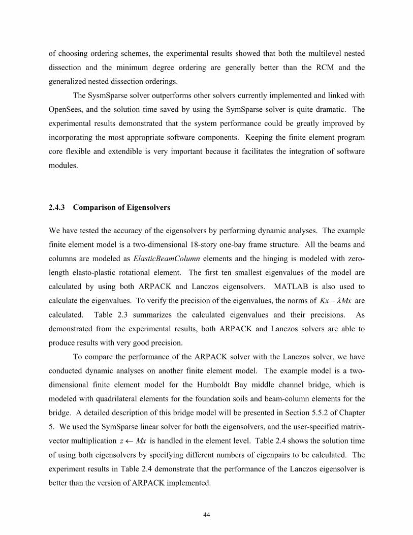
44
of choosing ordering schemes, the experimental results showed that both the multilevel nested
dissection and the minimum degree ordering are generally better than the RCM and the
generalized nested dissection orderings.
The SysmSparse solver outperforms other solvers currently implemented and linked with
OpenSees, and the solution time saved by using the SymSparse solver is quite dramatic. The
experimental results demonstrated that the system performance could be greatly improved by
incorporating the most appropriate software components. Keeping the finite element program
core flexible and extendible is very important because it facilitates the integration of software
modules.
2.4.3 Comparison of Eigensolvers
We have tested the accuracy of the eigensolvers by performing dynamic analyses. The example
finite element model is a two-dimensional 18-story one-bay frame structure. All the beams and
columns are modeled as ElasticBeamColumn elements and the hinging is modeled with zero-
length elasto-plastic rotational element. The first ten smallest eigenvalues of the model are
calculated by using both ARPACK and Lanczos eigensolvers. MATLAB is also used to
calculate the eigenvalues. To verify the precision of the eigenvalues, the norms of MxKx λ− are
calculated. Table 2.3 summarizes the calculated eigenvalues and their precisions. As
demonstrated from the experimental results, both ARPACK and Lanczos solvers are able to
produce results with very good precision.
To compare the performance of the ARPACK solver with the Lanczos solver, we have
conducted dynamic analyses on another finite element model. The example model is a two-
dimensional finite element model for the Humboldt Bay middle channel bridge, which is
modeled with quadrilateral elements for the foundation soils and beam-column elements for the
bridge. A detailed description of this bridge model will be presented in Section 5.5.2 of Chapter
5. We used the SymSparse linear solver for both the eigensolvers, and the user-specified matrix-
vector multiplication Mxz ← is handled in the element level. Table 2.4 shows the solution time
of using both eigensolvers by specifying different numbers of eigenpairs to be calculated. The
experiment results in Table 2.4 demonstrate that the performance of the Lanczos eigensolver is
better than the version of ARPACK implemented.
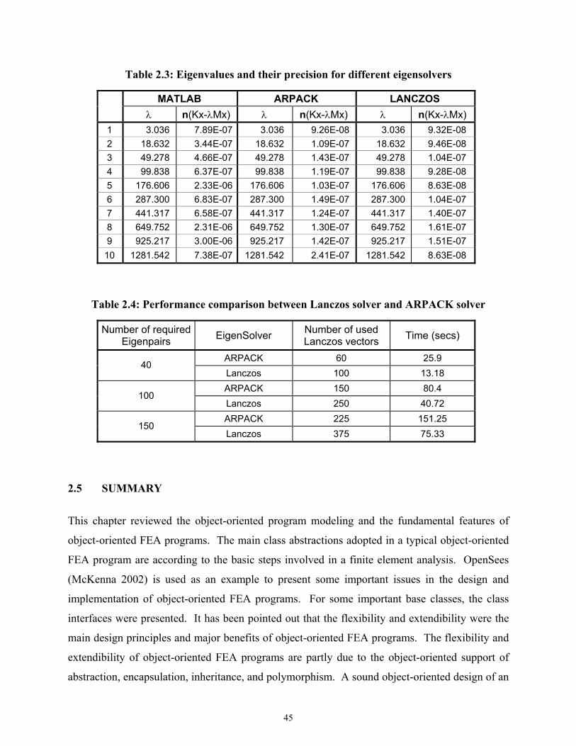
45
Table 2.3: Eigenvalues and their precision for different eigensolvers
MATLAB ARPACK LANCZOS λ n(Kx-λMx) λ n(Kx-λMx) λ n(Kx-λMx)
1 3.036 7.89E-07 3.036 9.26E-08 3.036 9.32E-08 2 18.632 3.44E-07 18.632 1.09E-07 18.632 9.46E-08 3 49.278 4.66E-07 49.278 1.43E-07 49.278 1.04E-07 4 99.838 6.37E-07 99.838 1.19E-07 99.838 9.28E-08 5 176.606 2.33E-06 176.606 1.03E-07 176.606 8.63E-08 6 287.300 6.83E-07 287.300 1.49E-07 287.300 1.04E-07 7 441.317 6.58E-07 441.317 1.24E-07 441.317 1.40E-07 8 649.752 2.31E-06 649.752 1.30E-07 649.752 1.61E-07 9 925.217 3.00E-06 925.217 1.42E-07 925.217 1.51E-07
10 1281.542 7.38E-07 1281.542 2.41E-07 1281.542 8.63E-08
Table 2.4: Performance comparison between Lanczos solver and ARPACK solver
Number of required Eigenpairs EigenSolver Number of used
Lanczos vectors Time (secs)
ARPACK 60 25.9 40
Lanczos 100 13.18 ARPACK 150 80.4
100 Lanczos 250 40.72 ARPACK 225 151.25
150 Lanczos 375 75.33
2.5 SUMMARY
This chapter reviewed the object-oriented program modeling and the fundamental features of
object-oriented FEA programs. The main class abstractions adopted in a typical object-oriented
FEA program are according to the basic steps involved in a finite element analysis. OpenSees
(McKenna 2002) is used as an example to present some important issues in the design and
implementation of object-oriented FEA programs. For some important base classes, the class
interfaces were presented. It has been pointed out that the flexibility and extendibility were the
main design principles and major benefits of object-oriented FEA programs. The flexibility and
extendibility of object-oriented FEA programs are partly due to the object-oriented support of
abstraction, encapsulation, inheritance, and polymorphism. A sound object-oriented design of an
46
FEA program facilitates the integration of external modules, making the integration process
modular and component based.
The flexibility of extending object-oriented FEA programs to incorporate new
developments and existing modules has been illustrated with several examples. While the
technique described can be applied to any object-oriented FEA software program, the discussion
and implementation were focused on the OpenSees platform (McKenna 2002). We used
OpenSees as a testing platform to incorporate a new element (eight-node quadrilateral element),
a popular graph partitioning and ordering package (METIS (Karypis and Kumar 1998b)), a
sparse linear direct solver (SymSparse (Mackay et al. 1991)), and two eigensolvers (ARPACK
(Lehoucq et al. 1997) and Lanczos eigensolver)). Because the characteristics of these software
components are different, they need to be incorporated by means of different approaches. The
software extending process normally requires introducing one or several subclasses of the
existing base classes. In the case of integrating well-defined components, black-box approach
can be applied. For some legacy applications, tight integration may be unavoidable because the
interfaces of these legacy applications are not well defined. Reverse communication, which is a
flexible mechanism to allow users to choose the most appropriate data structures for the
problems, can also be applied to object-oriented FEA programs to facilitate the integration of
external components. Although there are a number of approaches to extend the existing object-
oriented FEA programs, one common feature is that the changes to the existing code tend to be
localized. The localized code change is very important as it substantially reduces the efforts of
integrating components and minimizes the potentials of bugs being introduced.
After the software components are seamlessly integrated with an object-oriented FEA
program, the capability and performance of the program can be greatly improved. As shown
from the experimental results presented in this chapter, the incorporation of eigensolvers has
provided dynamic analyses capabilities to the OpenSees core. The usage of the SymSparse
solver can substantially reduce the solution time for solving linear system of equations, which in
turn improves the solution of eigenvalue problems and nonlinear structural analyses. Well-
defined interfaces and extendable modules are important for the design of object-oriented FEA
programs, since these features can facilitate the integration of external components. The
incorporating of different types of components allows the user to pick and choose the most
appropriate components to solve a finite element problem.
3 Open Collaborative Software Framework
This chapter describes an Internet-enabled open software framework that would facilitate the
utilization and the collaborative development of structural analysis programs by taking
advantage of the Internet, distributed computing, database, and other advanced computing
technologies (Peng and Law 2000; Peng and Law 2002; Peng et al. 2000). A collaborative
system is one where multiple users or agents engage in a shared activity, usually from remote
locations. By utilizing the Internet as a communication avenue, the framework makes the
structural analysis programs more easily accessible to the end users, and also facilitates the
integration of new developments. As illustrated in the previous chapter, the ability to easily
incorporate new solution algorithms and strategies, especially new sparse solvers and
eigensolvers, greatly improves the capabilities and performances of structural analysis programs,
making the software platform more efficient for large-scale engineering simulations. In this
open collaborative framework, we focus on accessing a software platform and testing and
incorporating new developments from a remote site. The framework also adopts a commercial
off-the-shelf (COTS) database system, which can address the data management problems
encountered by the prevailing file-system-based engineering analysis software applications. The
Internet-enabled collaborative framework can potentially provide greater flexibility and
extendibility than traditional structural analysis software packages, which are typically packaged
individually.
The objective of this chapter is to provide an overview of the framework, its modular
design, and the interaction between the modules. The user interaction interfaces are then
presented with example usage. Details of core component modules will be described in
subsequent chapters. This chapter is organized as follows:
• Section 3.1 gives an overview of the collaborative framework. The architecture and the
mechanics of the collaborative framework are described in this section.
48
• Section 3.2 introduces the modular design of the collaborative framework. The
collaborative framework consists of six distinct component modules. The functionality of
the component modules and the interaction among them are briefly discussed.
• Section 3.3 describes the user interfaces to the collaborative software framework. The
details on two types of user interfaces, namely a web-based interface and a MATLAB-
based interface, are presented.
• Section 3.4 presents a simple but typical structural model that will be used as an
illustrative example to facilitate the discussion. The sample web-based interface and
MATLAB-based interface for analyzing the model are presented.
3.1 OVERVIEW OF THE COLLABORATIVE FRAMEWORK
The collaborative software framework is designed to provide researchers and engineers with easy
access to an analysis platform and to incorporate new element technologies, new algorithms, and
solution strategies for nonlinear dynamic analyses. Users and engineers can have direct access to
the analysis core and the analysis results by using a web browser or other application programs,
such as MATLAB. Researchers and developers can utilize the collaborative framework as a
common finite element analysis tool to build, test, and incorporate new developments. A set of
Internet-enabled communication protocols is defined to link external new components which can
be easily integrated into the collaborative framework through a plug-and-play environment.
For the utilization and development of the Internet-enabled collaborative framework,
many participants from different organizations are involved. There are end users whose main
purpose is to use the core platform as an analysis tool. There are analysts and researchers whose
focus is to develop new element and material technologies to enhance the framework. There are
also core developers who are working to incorporate new analysis and solution strategies and to
expand the analysis core. Since the participants of the collaborative framework play different
roles with different perspectives, the focus of the collaborative framework is to support the
communication and cooperation of users and researchers, and to facilitate the incorporation of
their developments into the framework.
49
3.1.1 System Architecture As discussed earlier, the software framework is designed to support multiple parties and
applications and the interaction among these participants. To integrate and link multiple
computer applications and parties, a suitable architecture is needed to define how the
components (applications or parties) are connected (Smith and Scherer 1999). The proposed
distributed and collaborative system architecture is a versatile, message-based, and modular
infrastructure that is intended to improve usability, flexibility, interoperability, and scalability as
compared to centralized computing.
The overall system architecture of the Internet-enabled collaborative framework is
schematically depicted in Figure 3.1. OpenSees (McKenna 1997) is employed as the finite
element software analysis core engine for the prototype implementation of the framework. The
architecture defines the dependency and the interaction among the participants.
• In this framework, the structural analysis core program is running on a central server as a
compute engine. A compute engine is a remote software program that takes a set of tasks
from clients, runs them, and returns the result. A parallel and distributed computing
environment can be employed in the central server to improve the system performance
and make it more suitable for large-scale engineering simulations. New analysis
strategies and solution strategies can be incorporated to improve the capabilities and
performance of the server, as illustrated in the previous chapter for the integration of
modules such as the sparse direct solver and the eigensolvers.
• In this collaborative system, users play the role of clients to the central finite element
compute engine. The users can have direct or remote access (one such avenue is the
Internet) to the core program through a web-based user interface or another application
program, such as MATLAB. The users can specify desirable features and methods
(element types, efficient solution methods, and analysis strategies) that have been
developed, tested, and contributed to the framework by other participants.
• For element developers, a standard interface/wrapper is defined for communicating the
element(s) with the analysis core. The element code can be written in languages such as
Fortran, C, C++ and/or Java as long as it conforms to the standard interface, which is a
set of predefined protocols to bridge the element code with the central server. If the
developer and the system administrator agree, the new element can be merged into the
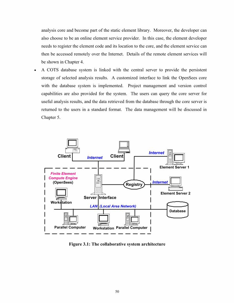
50
analysis core and become part of the static element library. Moreover, the developer can
also choose to be an online element service provider. In this case, the element developer
needs to register the element code and its location to the core, and the element service can
then be accessed remotely over the Internet. Details of the remote element services will
be shown in Chapter 4.
• A COTS database system is linked with the central server to provide the persistent
storage of selected analysis results. A customized interface to link the OpenSees core
with the database system is implemented. Project management and version control
capabilities are also provided for the system. The users can query the core server for
useful analysis results, and the data retrieved from the database through the core server is
returned to the users in a standard format. The data management will be discussed in
Chapter 5.
Workstation Parallel ComputerParallel Computer
Database
Element Server 2
Element Server 1
Registry
Finite ElementCompute Engine
(OpenSees)
InternetInternet
LAN (Local Area Network)
Internet
Server Interface
Client Client
Workstation
Figure 3.1: The collaborative system architecture
51
3.1.2 Mechanics
The mechanics of the open collaborative model are illustrated in Figure 3.2, which shows the
essential procedures to access the finite element compute engine and to perform structural
analyses over the Internet. First, a user of the system builds a structural model on the client site
and then submits it to the analysis core via a web-browser or an application program, using the
Internet as a communication channel. Upon receiving the model and other related information,
the core server authenticates the user’s identity and starts performing a structural analysis based
on the received model. Depending on the underlying hardware and system of the server core, the
analysis may be performed in a distributed and collaborative manner. During the analysis,
elements that are available in the core can be accessed locally from the static element library
(this is the case for most prevailing finite element packages), whereas other elements are
obtained from online element services. In order to find the required elements not existing in the
local element library, the registry is queried to find the location of the online element services,
which have been previously registered to the core platform. Once the online element services
have been identified and bound, the analysis core can access these element services in the same
way as they are located locally within the core. After the analysis is completed, part of the
results will be returned to the user by generating a dynamic web page displayed in the user’s web
browser.
The user can also query and view the analysis results using a web browser. The process
of analysis result query (postprocessing) follows almost the same procedures as performing an
analysis. Instead of submitting a structural model, the user submits a query to the server
platform. The core platform answers the query by returning certain results to the user, and this
process may involve database query and certain recomputation.
This section describes the use of a web browser for user interface to illustrate the
mechanics of the collaborative system. Besides the illustrated web-based interface, the user can
also interact with the core platform by using other application programs, such as MATLAB.
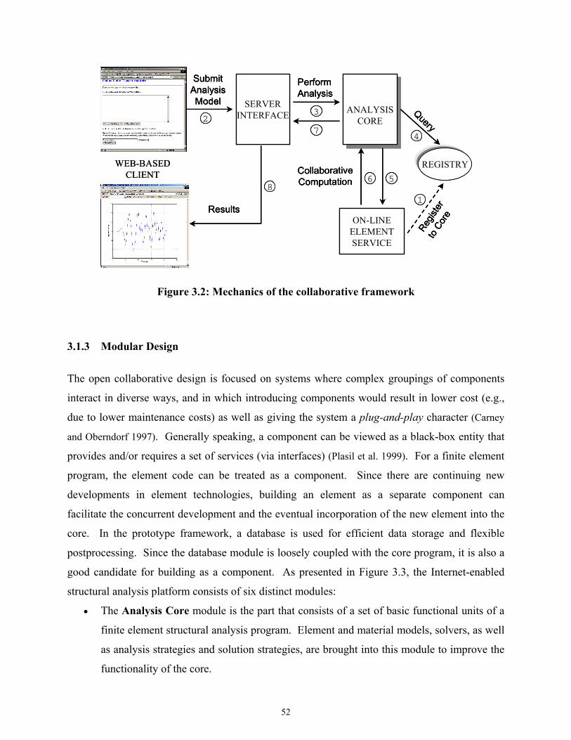
52
ANALYSISCORE
ANALYSISCORE
ON-LINEELEMENTSERVICE
REGISTRY
Query4
PerformAnalysis
3SERVER
INTERFACE
SubmitAnalysisModel
2
Regis
ter
to C
ore
1
CollaborativeComputation 6 5
WEB-BASEDCLIENT
Results
8
7
ANALYSISCORE
ANALYSISCORE
ON-LINEELEMENTSERVICE
REGISTRY
Query4
Query4
PerformAnalysis
3
PerformAnalysis
3SERVER
INTERFACE
SubmitAnalysisModel
2
SubmitAnalysisModel
2
Regis
ter
to C
ore
1
Regis
ter
to C
ore
1
CollaborativeComputation 6 5CollaborativeComputation 6 5
WEB-BASEDCLIENT
Results
8
7
Results
8
7
Figure 3.2: Mechanics of the collaborative framework
3.1.3 Modular Design
The open collaborative design is focused on systems where complex groupings of components
interact in diverse ways, and in which introducing components would result in lower cost (e.g.,
due to lower maintenance costs) as well as giving the system a plug-and-play character (Carney
and Oberndorf 1997). Generally speaking, a component can be viewed as a black-box entity that
provides and/or requires a set of services (via interfaces) (Plasil et al. 1999). For a finite element
program, the element code can be treated as a component. Since there are continuing new
developments in element technologies, building an element as a separate component can
facilitate the concurrent development and the eventual incorporation of the new element into the
core. In the prototype framework, a database is used for efficient data storage and flexible
postprocessing. Since the database module is loosely coupled with the core program, it is also a
good candidate for building as a component. As presented in Figure 3.3, the Internet-enabled
structural analysis platform consists of six distinct modules:
• The Analysis Core module is the part that consists of a set of basic functional units of a
finite element structural analysis program. Element and material models, solvers, as well
as analysis strategies and solution strategies, are brought into this module to improve the
functionality of the core.
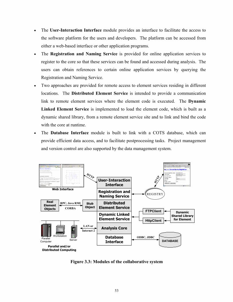
53
• The User-Interaction Interface module provides an interface to facilitate the access to
the software platform for the users and developers. The platform can be accessed from
either a web-based interface or other application programs.
• The Registration and Naming Service is provided for online application services to
register to the core so that these services can be found and accessed during analysis. The
users can obtain references to certain online application services by querying the
Registration and Naming Service.
• Two approaches are provided for remote access to element services residing in different
locations. The Distributed Element Service is intended to provide a communication
link to remote element services where the element code is executed. The Dynamic
Linked Element Service is implemented to load the element code, which is built as a
dynamic shared library, from a remote element service site and to link and bind the code
with the core at runtime.
• The Database Interface module is built to link with a COTS database, which can
provide efficient data access, and to facilitate postprocessing tasks. Project management
and version control are also supported by the data management system.
User-InteractionInterface
Registration andNaming Service
DistributedElement Service
Dynamic LinkedElement Service
Analysis Core
DatabaseInterface
REGISTRY
FTPClient
HttpClient
DynamicShared Library
for Element
RealElementObjects
StubObject
RPC, Java RMI
CORBA
HTTP
HTT
P
ODBC, JDBC
LAN orInternet 2
Parallel and/orDistributed Computing
DATABASE
Web Interface
ServerParallelComputer
Workstation
Figure 3.3: Modules of the collaborative system
54
3.2 USER INTERFACES
As shown in Figure 3.1, the collaborative framework can offer users access to the analysis core,
as well as the associated supporting services via the Internet. This client/server computing
environment consists of two logical parts: a server that provides services and a client that
requests services from the server. Together, the two parts form a complete computing
framework with a very distinct division of responsibility (Lewandowski 1998). One benefit of
this model is the transparency of software services. From a user’s perspective, the user deals
with a single service from a single point of contact — even though the actual structural analysis
may be performed in a distributed and collaborative manner. The other benefit is that this
framework can widen the reach of the analysis core to the users and external developers. The
core platform offering the finite element analysis service stays at the provider’s site, where the
software core is developed, kept securely, operated, maintained, and updated. Users can easily
access the software platform without the associated cost and maintenance challenges.
In the collaborative framework, the server core is based on a finite element analysis
program and a server interface is built to provide the network communication and data wrapping.
Java Servlet (Hunter and Crawford 2001) technology is employed to implement the server
interface, which serves as the wrapper to the OpenSees core. For the client application, COTS
software packages would be preferred as the user interface. There are two reasons for favoring
COTS software packages as user interfaces than developing a new GUI. First, COTS software
packages generally provide a friendly and easy-to-use interface to the users. Users are familiar
with the interfaces of popular and widely used software packages. Furthermore, many COTS
software packages normally have built-in facilities for developers to customize them. This
makes the development process more economical in terms of development time and efforts. In
the current collaborative framework, two types of user interfaces are provided: one is web based
and the other is MATLAB based.
3.2.1 OpenSees Tcl Input Interface
Since OpenSees is employed as the analysis core for the prototype implementation of the
collaborative framework, a brief review is given in the following for the input features of
55
OpenSees. However, the input features of OpenSees are not crucial to the building of the web-
based and MATLAB-based interfaces.
In order to conduct an analysis using the current version of OpenSees, most users need to
set up an input file. The input file can be parsed and interpreted by the OpenSees interpreter,
which is based on an extension of the scripting language Tcl (Tool Command Language)
(Ousterhout 1994). Tcl is a string-based procedural command language that supports
substitution, loops, mathematical expressions, and procedures. Besides defining a programmable
language, Tcl also has a library package. First, Tcl is a simple textual language, intended
primarily for issuing commands to interactive programs such as text editors, debuggers, and
shells. It has a simple syntax and is also programmable, so users can write command procedures
to provide more powerful commands than those in the built-in set. Second, Tcl is a library
package that can be embedded in application programs. The Tcl library consists of a parser for
the Tcl language, routines to implement the Tcl built-in commands, and procedures that allow
each application to extend Tcl with additional commands specific to that application. The
application program generates Tcl commands and passes them to the Tcl parser for execution.
When the Tcl library receives commands it parses them into component fields and executes
built-in commands directly. For commands implemented by the application, Tcl calls back to the
application to execute the commands.
For the implementation of the OpenSees interpreter, a Tcl library package is embedded in
OpenSees. The OpenSees interpreter adds commands to the standard Tcl for finite element
analysis. The OpenSees interpreter comprises a set of commands to create finite element
models, to specify an analysis procedure, to perform the analysis, and to output the results. Each
of these commands is associated (bound) with an OpenSees procedure or class. Thus the users
can use these commands to create an OpenSees object and invoke methods on that object. Most
of the classes in OpenSees have their corresponding Tcl commands, the details of which have
been described by McKenna and Fenves (McKenna and Fenves 2001).
Based on the defined Tcl commands, an input file can be created. A typical input file is
composed of a sequence of Tcl commands that controls the flow of a finite element analysis.
After the input file is submitted to the OpenSees interpreter, the commands in the file are parsed
and interpreted, and corresponding methods are invoked on OpenSees to execute the commands.
For example, once the interpreter receives the command element, it forwards the parameters of
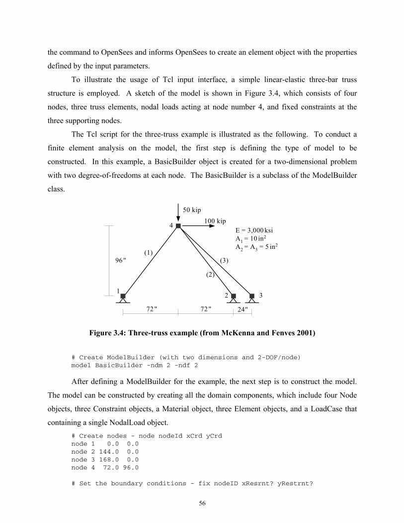
56
the command to OpenSees and informs OpenSees to create an element object with the properties
defined by the input parameters.
To illustrate the usage of Tcl input interface, a simple linear-elastic three-bar truss
structure is employed. A sketch of the model is shown in Figure 3.4, which consists of four
nodes, three truss elements, nodal loads acting at node number 4, and fixed constraints at the
three supporting nodes.
The Tcl script for the three-truss example is illustrated as the following. To conduct a
finite element analysis on the model, the first step is defining the type of model to be
constructed. In this example, a BasicBuilder object is created for a two-dimensional problem
with two degree-of-freedoms at each node. The BasicBuilder is a subclass of the ModelBuilder
class.
72 ''
96 ''
24 ''72 ''
50 kip100 kip
1
4
32
(1)(3)
(2)
E = 3,000 ksiA1 = 10 in2
A2 = A3 = 5 in2
Figure 3.4: Three-truss example (from McKenna and Fenves 2001)
# Create ModelBuilder (with two dimensions and 2-DOF/node) model BasicBuilder -ndm 2 -ndf 2
After defining a ModelBuilder for the example, the next step is to construct the model.
The model can be constructed by creating all the domain components, which include four Node
objects, three Constraint objects, a Material object, three Element objects, and a LoadCase that
containing a single NodalLoad object. # Create nodes - node nodeId xCrd yCrd node 1 0.0 0.0 node 2 144.0 0.0 node 3 168.0 0.0 node 4 72.0 96.0 # Set the boundary conditions - fix nodeID xResrnt? yRestrnt?
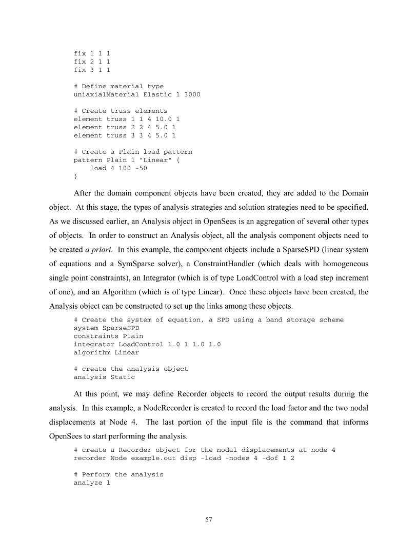
57
fix 1 1 1 fix 2 1 1 fix 3 1 1 # Define material type uniaxialMaterial Elastic 1 3000 # Create truss elements element truss 1 1 4 10.0 1 element truss 2 2 4 5.0 1 element truss 3 3 4 5.0 1 # Create a Plain load pattern pattern Plain 1 "Linear" { load 4 100 -50 }
After the domain component objects have been created, they are added to the Domain
object. At this stage, the types of analysis strategies and solution strategies need to be specified.
As we discussed earlier, an Analysis object in OpenSees is an aggregation of several other types
of objects. In order to construct an Analysis object, all the analysis component objects need to
be created a priori. In this example, the component objects include a SparseSPD (linear system
of equations and a SymSparse solver), a ConstraintHandler (which deals with homogeneous
single point constraints), an Integrator (which is of type LoadControl with a load step increment
of one), and an Algorithm (which is of type Linear). Once these objects have been created, the
Analysis object can be constructed to set up the links among these objects. # Create the system of equation, a SPD using a band storage scheme system SparseSPD constraints Plain integrator LoadControl 1.0 1 1.0 1.0 algorithm Linear # create the analysis object analysis Static
At this point, we may define Recorder objects to record the output results during the
analysis. In this example, a NodeRecorder is created to record the load factor and the two nodal
displacements at Node 4. The last portion of the input file is the command that informs
OpenSees to start performing the analysis. # create a Recorder object for the nodal displacements at node 4 recorder Node example.out disp -load -nodes 4 -dof 1 2 # Perform the analysis analyze 1
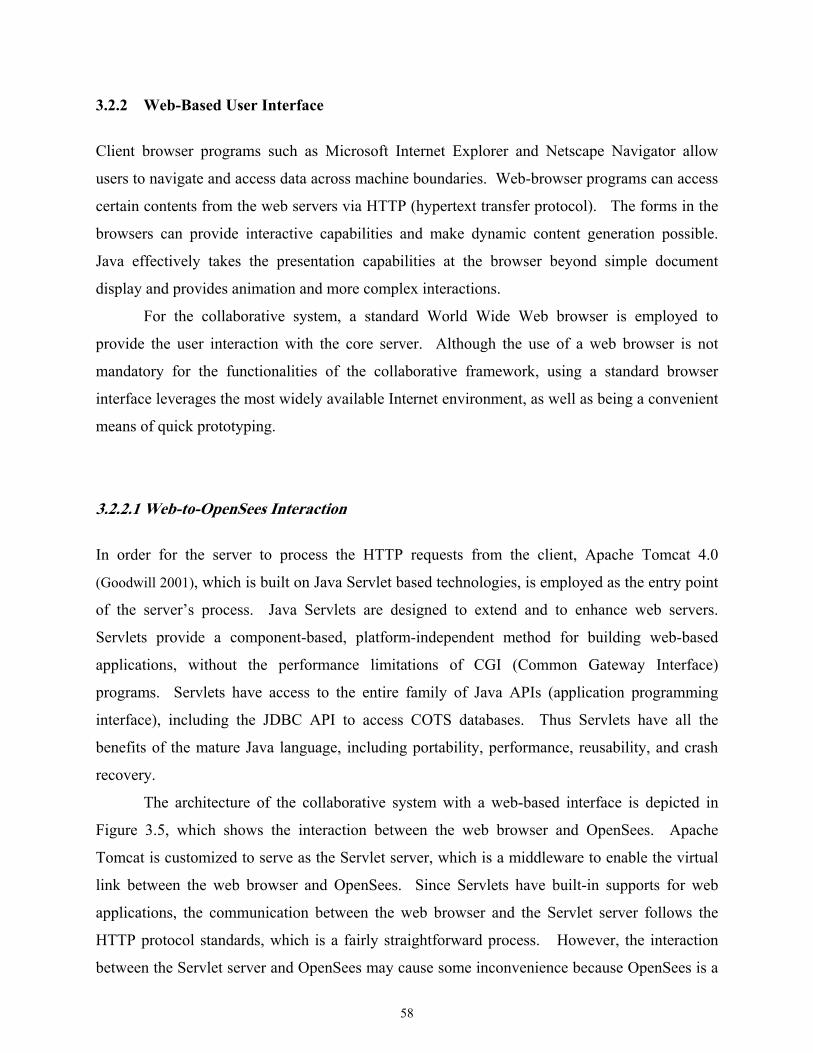
58
3.2.2 Web-Based User Interface
Client browser programs such as Microsoft Internet Explorer and Netscape Navigator allow
users to navigate and access data across machine boundaries. Web-browser programs can access
certain contents from the web servers via HTTP (hypertext transfer protocol). The forms in the
browsers can provide interactive capabilities and make dynamic content generation possible.
Java effectively takes the presentation capabilities at the browser beyond simple document
display and provides animation and more complex interactions.
For the collaborative system, a standard World Wide Web browser is employed to
provide the user interaction with the core server. Although the use of a web browser is not
mandatory for the functionalities of the collaborative framework, using a standard browser
interface leverages the most widely available Internet environment, as well as being a convenient
means of quick prototyping.
3.2.2.1 Web-to-OpenSees Interaction
In order for the server to process the HTTP requests from the client, Apache Tomcat 4.0
(Goodwill 2001), which is built on Java Servlet based technologies, is employed as the entry point
of the server’s process. Java Servlets are designed to extend and to enhance web servers.
Servlets provide a component-based, platform-independent method for building web-based
applications, without the performance limitations of CGI (Common Gateway Interface)
programs. Servlets have access to the entire family of Java APIs (application programming
interface), including the JDBC API to access COTS databases. Thus Servlets have all the
benefits of the mature Java language, including portability, performance, reusability, and crash
recovery.
The architecture of the collaborative system with a web-based interface is depicted in
Figure 3.5, which shows the interaction between the web browser and OpenSees. Apache
Tomcat is customized to serve as the Servlet server, which is a middleware to enable the virtual
link between the web browser and OpenSees. Since Servlets have built-in supports for web
applications, the communication between the web browser and the Servlet server follows the
HTTP protocol standards, which is a fairly straightforward process. However, the interaction
between the Servlet server and OpenSees may cause some inconvenience because OpenSees is a
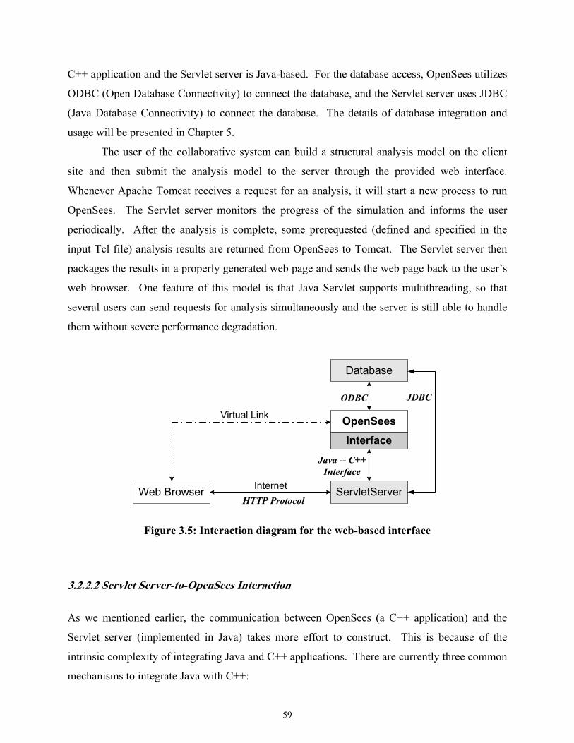
59
C++ application and the Servlet server is Java-based. For the database access, OpenSees utilizes
ODBC (Open Database Connectivity) to connect the database, and the Servlet server uses JDBC
(Java Database Connectivity) to connect the database. The details of database integration and
usage will be presented in Chapter 5.
The user of the collaborative system can build a structural analysis model on the client
site and then submit the analysis model to the server through the provided web interface.
Whenever Apache Tomcat receives a request for an analysis, it will start a new process to run
OpenSees. The Servlet server monitors the progress of the simulation and informs the user
periodically. After the analysis is complete, some prerequested (defined and specified in the
input Tcl file) analysis results are returned from OpenSees to Tomcat. The Servlet server then
packages the results in a properly generated web page and sends the web page back to the user’s
web browser. One feature of this model is that Java Servlet supports multithreading, so that
several users can send requests for analysis simultaneously and the server is still able to handle
them without severe performance degradation.
Web Browser ServletServer
OpenSees
Interface
Internet
Virtual Link
Database
HTTP Protocol
ODBC JDBC
Java -- C++Interface
Figure 3.5: Interaction diagram for the web-based interface
3.2.2.2 Servlet Server-to-OpenSees Interaction
As we mentioned earlier, the communication between OpenSees (a C++ application) and the
Servlet server (implemented in Java) takes more effort to construct. This is because of the
intrinsic complexity of integrating Java and C++ applications. There are currently three common
mechanisms to integrate Java with C++:
60
• External process: Every Java application has a single instance of class Runtime that
allows the Java application to interface with an external process in which a C++
application can be running. This is the most straightforward way for a Java application to
interact with a stand-alone application written in other languages. The Java API provides
methods for performing input from the process, performing output to the process, waiting
for the process to complete, checking the exit status of the process, and destroying the
process.
• JNI: The Java Native Interface (Liang 1999) is the native programming interface for Java
that allows Java code running within a Java Virtual Machine (VM) to operate with
applications and libraries written in other languages, such as C, C++, Fortran, or
assembly. In addition, the Invocation API allows the embedding of a Java Virtual
Machine into native applications. The JNI framework supports native objects to utilize
Java objects in the same way that Java code uses these objects. Thus, both the
application written in native languages and Java application can create, update, and
access Java objects and then share these objects between them.
• Sockets: For each network communication pair, the source and destination processes can
be uniquely identified by their IP addresses and port numbers. The combination of an IP
address and a port number is called a “socket.” Both Java and C++ have socket classes to
construct communication with external processes, which can be on the same computer or
on a different computer that connected with some sort of network. The integration
between Java and C++ applications can be achieved by utilizing socket classes to build a
communication channel.
All the three modes of integrating Java and C++ applications are utilized in the
collaborative framework because each of them has certain advantages and can be applied in
different situations. The External Process method is the easiest to implement and is relatively
robust, but the communication between Java and external process is limited to standard
Input/Output. This mode is applied for the Servlet server to invoke an OpenSees process and to
submit an analysis model to OpenSees. The JNI framework provides fairly complete, but tightly
coupled connection between Java and external processes. The distributed element service relies
on the support of JNI, and the details of distributed element service will be explained in Chapter
4. The Sockets connection has a clear distinction between source and destination, and thus it
helps to keep the connection between Java and C++ applications clear and loosely coupled.
61
For a typical structural analysis software package, the user interface needs to support at
least two types of operations. One is invoking the analysis and the other is postprocessing,
which is mainly dealing with analysis results query. The collaborative framework can also
provide these two types of operations. For invoking an OpenSees process and transferring the
analysis model, the Servlet server utilizes the External Process mode to communication with
OpenSees core. For the support of postprocessing, the Servlet server exchanges data with
OpenSees via a Socket connection.
3.2.3 MATLAB-Based User Interface
For web-based services, all too often the analysis result is downloaded from the computational
server as a file, and then put manually (cut and paste plus maybe some cumbersome conversions)
into another program, e.g., a spreadsheet, to perform postprocessing. For example, if we want to
plot a time history response from a dynamic analysis, we might have to download the response in
a data file and then use MATLAB, Excel, or other software packages to generate the graphical
representation. This ad hoc manual process might also involve data format conversion and
software system configuration. It would be more convenient to directly utilize some popular
application software packages to enhance the user interaction with the collaborative system core,
eliminating the cumbersome interim manual procedures. In the collaborative system framework,
besides the web-based user interface, a MATLAB-based user interface is developed as an
alternative and enhancement for the user interaction. The combination of the intuitive MATLAB
interface, language, and the built-in math and graphics functions makes MATLAB the preferred
platform for scientific computing compared to C, Fortran, and other applications.
The client-side MATLAB service is very flexible and very powerful, and it allows
customization for the users. In the current implementation, some extra functions are added to the
standard MATLAB for handling the network communication and data processing. These
functions are sufficient to perform basic finite element analysis together with certain
postprocessing capabilities. These add-on functions can be directly invoked from either the
standard MATLAB prompt or a MATLAB-based GUI (graphical user interface). The add-on
functions can be categorized in the following groups:
• submitfile, submitmodel: Analysis model submission and analysis invocation;
62
• dataquery: Analysis results query;
• modelplot, deformedplot, res2Dplot: Postprocessing.
In the prototype system, we chose MATLAB because of its build-in support and its
popularity and availability. However, MATLAB is not the only candidate for building a user
interface. Similar network communication protocols and data processing tools can be built for
other application programs, such as FEA postprocessing packages or Excel.
3.2.3.1 Network Communication
As stated previously, a Java Servlet-enabled server is employed as the middleware between
clients and the OpenSees core. The Servlet server supports protocols that are specified as rules
and conventions for communication. Although the protocols are originally defined for web
browser-based clients, they are applicable to any software system that speaks the same language.
To incorporate MATLAB as a client to the collaborative software framework, a wrapper is
needed to handle the network communication for MATLAB. The wrapper can be implemented
to conform to the defined Servlet server protocols; thus the same Servlet server can interoperate
with both web client and MATLAB client. This approach eliminates the modifications to the
existing Servlet server.
Figure 3.6 shows the interaction between MATLAB and OpenSees. The server
implementation and configuration are the same as those of the server for a web-based client.
MATLAB and MATLAB-enabled GUI (graphical user interface) interact with the ServletServer
through a Java client, which is provided to make the network communication conform to the
existing server protocol. The communication channel between the JavaClient and the
ServletServer can be any popular network media, preferably the Internet. Through this layered
architecture, a virtual link is established between MATLAB and OpenSees.
The link between MATLAB and the JavaClient is supported by the MATLAB Java
Interface, which is a new built-in component of MATLAB to interface with Java classes and
objects. Every installation of MATLAB includes a Java Virtual Machine (JVM), so that we can
use the Java interpreter via MATLAB commands, and we can create and run programs that
create and access Java objects. This MATLAB capability enables us to conveniently bring Java
classes into the MATLAB environment, to construct objects from those classes, to call methods
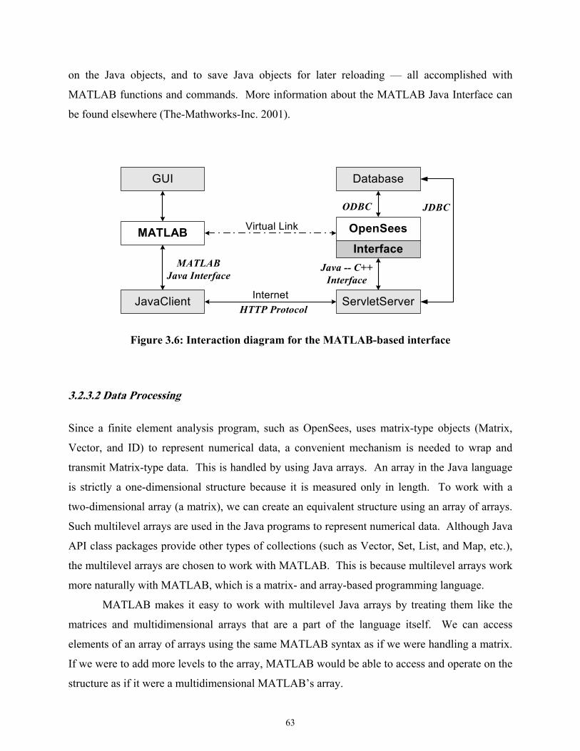
63
on the Java objects, and to save Java objects for later reloading — all accomplished with
MATLAB functions and commands. More information about the MATLAB Java Interface can
be found elsewhere (The-Mathworks-Inc. 2001).
JavaClient ServletServer
OpenSeesMATLABInterface
Internet
Virtual Link
DatabaseGUI
ODBC
HTTP Protocol
JDBC
MATLABJava Interface
Java -- C++Interface
Figure 3.6: Interaction diagram for the MATLAB-based interface
3.2.3.2 Data Processing
Since a finite element analysis program, such as OpenSees, uses matrix-type objects (Matrix,
Vector, and ID) to represent numerical data, a convenient mechanism is needed to wrap and
transmit Matrix-type data. This is handled by using Java arrays. An array in the Java language
is strictly a one-dimensional structure because it is measured only in length. To work with a
two-dimensional array (a matrix), we can create an equivalent structure using an array of arrays.
Such multilevel arrays are used in the Java programs to represent numerical data. Although Java
API class packages provide other types of collections (such as Vector, Set, List, and Map, etc.),
the multilevel arrays are chosen to work with MATLAB. This is because multilevel arrays work
more naturally with MATLAB, which is a matrix- and array-based programming language.
MATLAB makes it easy to work with multilevel Java arrays by treating them like the
matrices and multidimensional arrays that are a part of the language itself. We can access
elements of an array of arrays using the same MATLAB syntax as if we were handling a matrix.
If we were to add more levels to the array, MATLAB would be able to access and operate on the
structure as if it were a multidimensional MATLAB’s array.
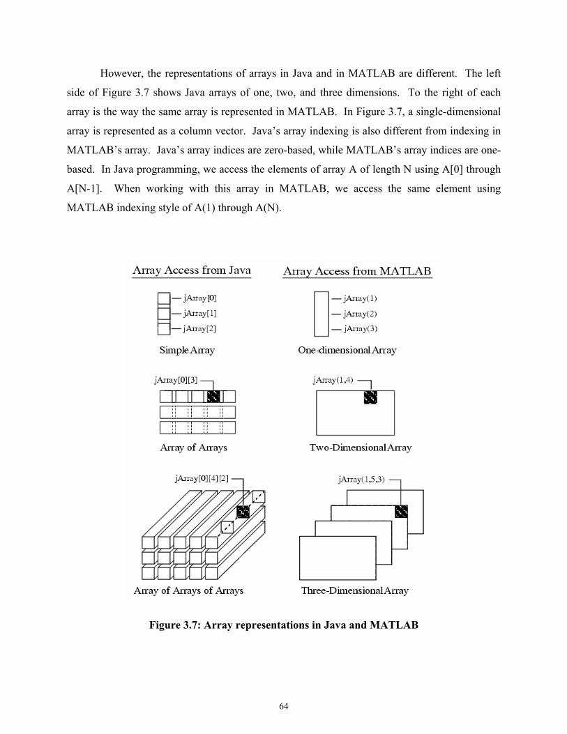
64
However, the representations of arrays in Java and in MATLAB are different. The left
side of Figure 3.7 shows Java arrays of one, two, and three dimensions. To the right of each
array is the way the same array is represented in MATLAB. In Figure 3.7, a single-dimensional
array is represented as a column vector. Java’s array indexing is also different from indexing in
MATLAB’s array. Java’s array indices are zero-based, while MATLAB’s array indices are one-
based. In Java programming, we access the elements of array A of length N using A[0] through
A[N-1]. When working with this array in MATLAB, we access the same element using
MATLAB indexing style of A(1) through A(N).
Figure 3.7: Array representations in Java and MATLAB
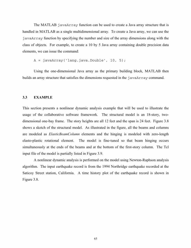
65
The MATLAB javaArray function can be used to create a Java array structure that is
handled in MATLAB as a single multidimensional array. To create a Java array, we can use the
javaArray function by specifying the number and size of the array dimensions along with the
class of objects. For example, to create a 10 by 5 Java array containing double precision data
elements, we can issue the command:
A = javaArray(‘lang.java.Double’, 10, 5);
Using the one-dimensional Java array as the primary building block, MATLAB then
builds an array structure that satisfies the dimensions requested in the javaArray command.
3.3 EXAMPLE
This section presents a nonlinear dynamic analysis example that will be used to illustrate the
usage of the collaborative software framework. The structural model is an 18-story, two-
dimensional one-bay frame. The story heights are all 12 feet and the span is 24 feet. Figure 3.8
shows a sketch of the structural model. As illustrated in the figure, all the beams and columns
are modeled as ElasticBeamColumn elements and the hinging is modeled with zero-length
elasto-plastic rotational element. The model is fine-tuned so that beam hinging occurs
simultaneously at the ends of the beams and at the bottom of the first-story column. The Tcl
input file of the model is partially listed in Figure 3.9.
A nonlinear dynamic analysis is performed on the model using Newton-Raphson analysis
algorithm. The input earthquake record is from the 1994 Northridge earthquake recorded at the
Saticoy Street station, California. A time history plot of the earthquake record is shown in
Figure 3.8.
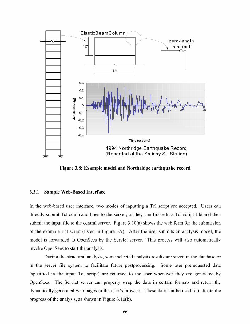
66
-0.4
-0.3
-0.2
-0.1
0
0.1
0.2
0.3
0 5 10 15 20 25
Time (second)
Acc
eler
atio
n (g
)
12'
24'
zero-lengthelement
ElasticBeamColumn
1994 Northridge Earthquake Record(Recorded at the Saticoy St. Station)
Figure 3.8: Example model and Northridge earthquake record
3.3.1 Sample Web-Based Interface
In the web-based user interface, two modes of inputting a Tcl script are accepted. Users can
directly submit Tcl command lines to the server; or they can first edit a Tcl script file and then
submit the input file to the central server. Figure 3.10(a) shows the web form for the submission
of the example Tcl script (listed in Figure 3.9). After the user submits an analysis model, the
model is forwarded to OpenSees by the Servlet server. This process will also automatically
invoke OpenSees to start the analysis.
During the structural analysis, some selected analysis results are saved in the database or
in the server file system to facilitate future postprocessing. Some user prerequested data
(specified in the input Tcl script) are returned to the user whenever they are generated by
OpenSees. The Servlet server can properly wrap the data in certain formats and return the
dynamically generated web pages to the user’s browser. These data can be used to indicate the
progress of the analysis, as shown in Figure 3.10(b).
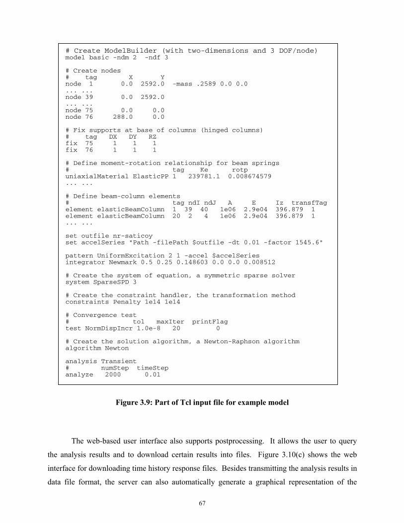
67
# Create ModelBuilder (with two-dimensions and 3 DOF/node) model basic -ndm 2 -ndf 3 # Create nodes # tag X Y node 1 0.0 2592.0 -mass .2589 0.0 0.0 ... ... node 39 0.0 2592.0 ... ... node 75 0.0 0.0 node 76 288.0 0.0 # Fix supports at base of columns (hinged columns) # tag DX DY RZ fix 75 1 1 1 fix 76 1 1 1 # Define moment-rotation relationship for beam springs # tag Ke rotp uniaxialMaterial ElasticPP 1 239781.1 0.008674579 ... ... # Define beam-column elements # tag ndI ndJ A E Iz transfTag element elasticBeamColumn 1 39 40 1e06 2.9e04 396.879 1 element elasticBeamColumn 20 2 4 1e06 2.9e04 396.879 1 ... ... set outfile nr-saticoy set accelSeries "Path -filePath $outfile -dt 0.01 -factor 1545.6" pattern UniformExcitation 2 1 -accel $accelSeries integrator Newmark 0.5 0.25 0.148603 0.0 0.0 0.008512 # Create the system of equation, a symmetric sparse solver system SparseSPD 3 # Create the constraint handler, the transformation method constraints Penalty 1e14 1e14 # Convergence test # tol maxIter printFlag test NormDispIncr 1.0e-8 20 0 # Create the solution algorithm, a Newton-Raphson algorithm algorithm Newton analysis Transient # numStep timeStep analyze 2000 0.01
Figure 3.9: Part of Tcl input file for example model
The web-based user interface also supports postprocessing. It allows the user to query
the analysis results and to download certain results into files. Figure 3.10(c) shows the web
interface for downloading time history response files. Besides transmitting the analysis results in
data file format, the server can also automatically generate a graphical representation of the
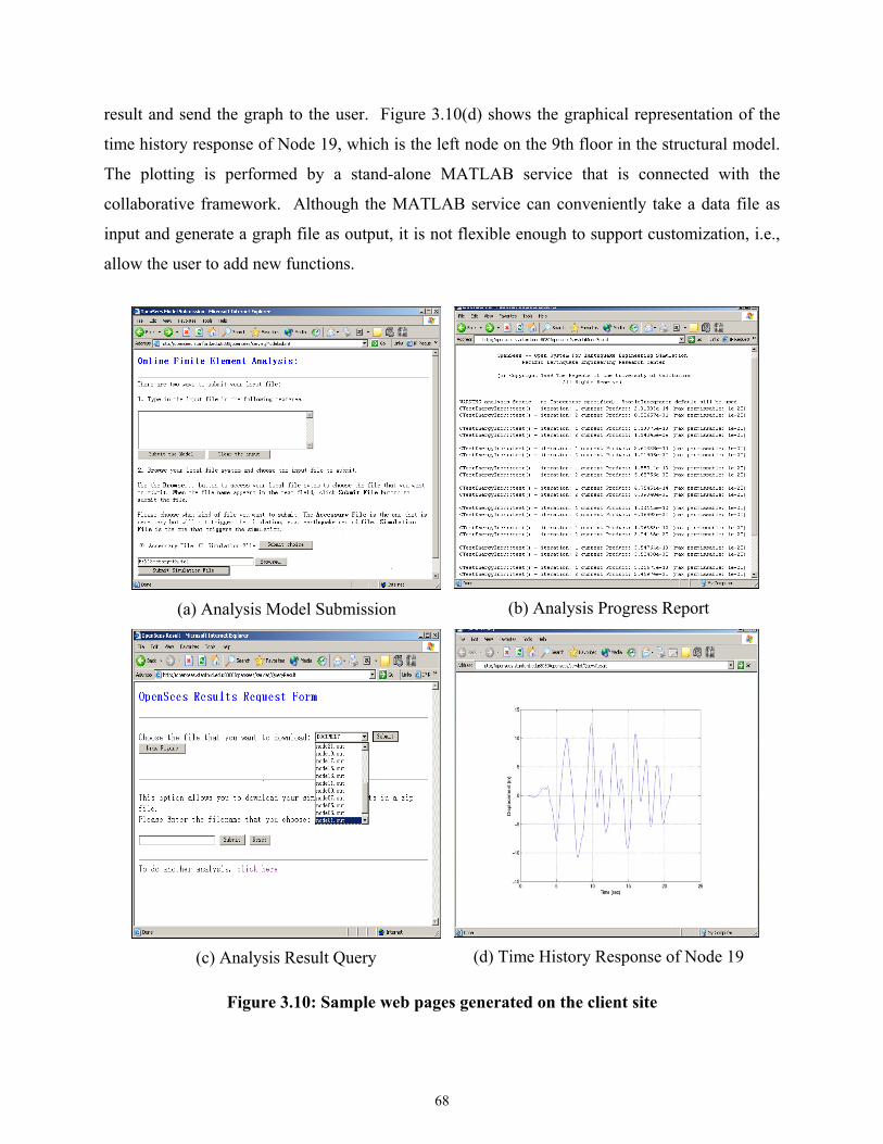
68
result and send the graph to the user. Figure 3.10(d) shows the graphical representation of the
time history response of Node 19, which is the left node on the 9th floor in the structural model.
The plotting is performed by a stand-alone MATLAB service that is connected with the
collaborative framework. Although the MATLAB service can conveniently take a data file as
input and generate a graph file as output, it is not flexible enough to support customization, i.e.,
allow the user to add new functions.
(a) Analysis Model Submission
(b) Analysis Progress Report
(c) Analysis Result Query (d) Time History Response of Node 19
Figure 3.10: Sample web pages generated on the client site
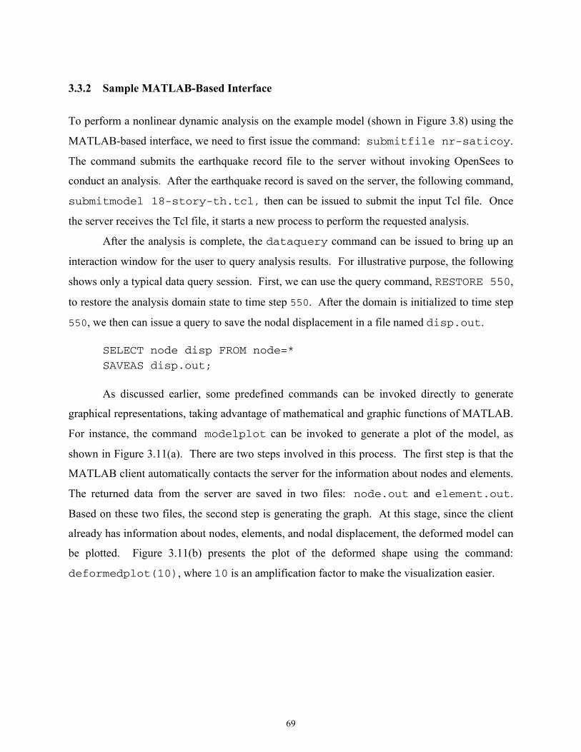
69
3.3.2 Sample MATLAB-Based Interface
To perform a nonlinear dynamic analysis on the example model (shown in Figure 3.8) using the
MATLAB-based interface, we need to first issue the command: submitfile nr-saticoy.
The command submits the earthquake record file to the server without invoking OpenSees to
conduct an analysis. After the earthquake record is saved on the server, the following command,
submitmodel 18-story-th.tcl, then can be issued to submit the input Tcl file. Once
the server receives the Tcl file, it starts a new process to perform the requested analysis.
After the analysis is complete, the dataquery command can be issued to bring up an
interaction window for the user to query analysis results. For illustrative purpose, the following
shows only a typical data query session. First, we can use the query command, RESTORE 550,
to restore the analysis domain state to time step 550. After the domain is initialized to time step
550, we then can issue a query to save the nodal displacement in a file named disp.out.
SELECT node disp FROM node=*
SAVEAS disp.out;
As discussed earlier, some predefined commands can be invoked directly to generate
graphical representations, taking advantage of mathematical and graphic functions of MATLAB.
For instance, the command modelplot can be invoked to generate a plot of the model, as
shown in Figure 3.11(a). There are two steps involved in this process. The first step is that the
MATLAB client automatically contacts the server for the information about nodes and elements.
The returned data from the server are saved in two files: node.out and element.out.
Based on these two files, the second step is generating the graph. At this stage, since the client
already has information about nodes, elements, and nodal displacement, the deformed model can
be plotted. Figure 3.11(b) presents the plot of the deformed shape using the command:
deformedplot(10), where 10 is an amplification factor to make the visualization easier.
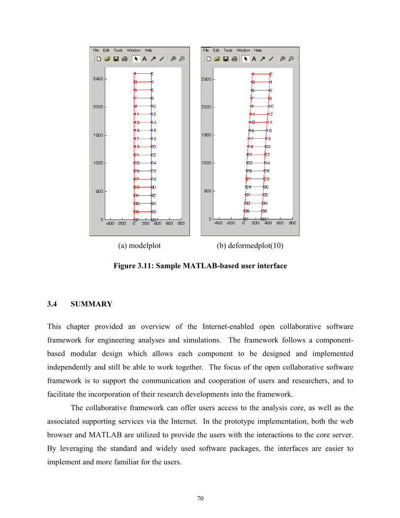
70
(a) modelplot
(b) deformedplot(10)
Figure 3.11: Sample MATLAB-based user interface
3.4 SUMMARY
This chapter provided an overview of the Internet-enabled open collaborative software
framework for engineering analyses and simulations. The framework follows a component-
based modular design which allows each component to be designed and implemented
independently and still be able to work together. The focus of the open collaborative software
framework is to support the communication and cooperation of users and researchers, and to
facilitate the incorporation of their research developments into the framework.
The collaborative framework can offer users access to the analysis core, as well as the
associated supporting services via the Internet. In the prototype implementation, both the web
browser and MATLAB are utilized to provide the users with the interactions to the core server.
By leveraging the standard and widely used software packages, the interfaces are easier to
implement and more familiar for the users.
71
The Internet-enabled open collaborative engineering software for analysis and simulation
has at least three benefits. First, the platform provides a means of distributing services in a
modular and systematic way. The modular service model helps the integration of legacy code as
one of the modular services in the infrastructure. Users can select appropriate services and can
easily replace a service by another one, without having to recompile the existing services being
used. Secondly, the client-server nature of the framework makes it possible for the end users to
take advantage of the server computing environment, where the distributed and parallel
computing environment can be utilized to facilitate large-scale engineering simulations. Finally,
the framework alleviates the burden of managing a group of developers and their source code.
Once a common communication protocol is defined, participants can develop the code in
compliance with the protocol. The need to constantly merge the code written by different
participants can be alleviated.
4 Internet-Enabled Service Integration and Communication
One of the salient features of the open collaborative software framework is to facilitate analysts
to integrate new developments with the core server so that the functionalities of the analysis core
can be enhanced. The Internet-enabled collaborative service architecture would allow new
application services to be incorporated with the analysis core in a dynamic and distributed
manner. A diverse group of users and developers can easily access the platform and contribute
their own developments to the central core. By providing a modular infrastructure, services can
be added or updated without the recompilation or reinitialization of the existing services. For
illustration purposes, this chapter focuses on the model integration of new elements to the
analysis core of OpenSees. There are two types of online element services: namely, distributed
element service and dynamic shared library element service. The infrastructure for supporting
the integration of these two types of online element service is presented. Similar infrastructure
and communication protocol can be designed and implemented to link other types of online
modular services, e.g., material services, solution algorithms services, and analysis strategies
services, etc. OpenSees is employed as the finite element analysis core in the prototype
implementation.
In order to build an Internet-enabled service framework for an object-oriented FEA
program such as OpenSees, a standard interface/wrapper needs to be defined for communicating
the online element services with the analysis core. The standard interface can facilitate the
concurrent development of new elements, and allow the replacement of an existing element code
if a superior one becomes available. The encapsulation and inheritance features of object-
oriented programming are utilized to define the standard interface for the element. As discussed
in Chapter 2, a super-class Element is provided in an object-oriented FEA program kernel (for
details about the Element class in OpenSees, see (McKenna 1997), which defines the essential
74
methods that an element needs to support. The traditional way of introducing a new element into
the object-oriented FEA program is to create a subclass of the Element class and possibly use the
new class to encapsulate the code related to the new element. The new element code, once tested
and approved for adoption, becomes part of the core’s static element library. For the Internet-
enabled collaborative framework, the code developer can also choose to be an online element
service provider. Two forms of online element services, namely distributed element service and
dynamic shared library element service, are introduced in the collaborative framework. Which
form of service to be used for linking the element with the core is up to the developers for their
convenience and other considerations. As long as the new element conforms to the standard
interface, it will be able to communicate with the analysis core. As opposed to the traditional
statically linked element library, the online element services will not expose the source code to
the core. Therefore, the collaborative platform allows the building of proprietary element
services and facilitates the linking of legacy applications.
The online element service can be released to public use by registering itself to the
Registration and Naming Service (RANS) with its name, location, service type (whether a
distributed service or a dynamic shared library service), and other pertinent information. During
a structural analysis, the RANS can be queried to find the appropriate type and location of the
requested element service. Although there are three types of element services (static element
library and two forms of online element services), the selection and binding of element services
are automatic and completely transparent to the users. The end users do not need to know the
type of element service to choose, nor do they need to be aware of the location of the service.
In this chapter, we describe in detail the development of an application service and its
integration with the Internet-enabled finite element analysis framework. This chapter is
organized as follows:
• Section 4.1 describes the registration and naming service (RANS) for the Internet-
enabled collaborative framework. The design and the implementation of the RANS
server are presented.
• Section 4.2 provides a detailed description of the distributed element service. The
mechanics of the distributed element service, the interaction of distributed applications
with the analysis core, and the implementation of the distributed element service are
presented in this section.
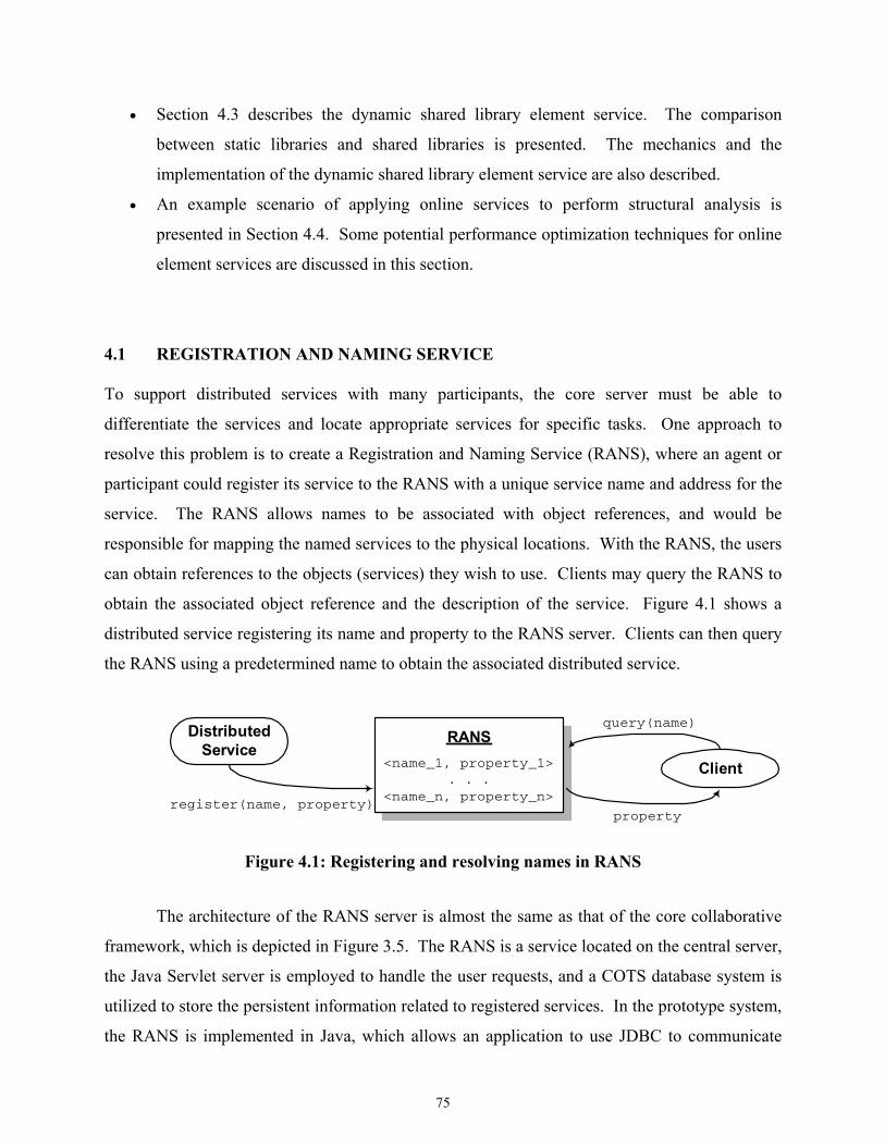
75
• Section 4.3 describes the dynamic shared library element service. The comparison
between static libraries and shared libraries is presented. The mechanics and the
implementation of the dynamic shared library element service are also described.
• An example scenario of applying online services to perform structural analysis is
presented in Section 4.4. Some potential performance optimization techniques for online
element services are discussed in this section.
4.1 REGISTRATION AND NAMING SERVICE To support distributed services with many participants, the core server must be able to
differentiate the services and locate appropriate services for specific tasks. One approach to
resolve this problem is to create a Registration and Naming Service (RANS), where an agent or
participant could register its service to the RANS with a unique service name and address for the
service. The RANS allows names to be associated with object references, and would be
responsible for mapping the named services to the physical locations. With the RANS, the users
can obtain references to the objects (services) they wish to use. Clients may query the RANS to
obtain the associated object reference and the description of the service. Figure 4.1 shows a
distributed service registering its name and property to the RANS server. Clients can then query
the RANS using a predetermined name to obtain the associated distributed service.
<name_1, property_1>. . .
<name_n, property_n>
<name_1, property_1>. . .
<name_n, property_n>
RANS
Client
DistributedService
register(name, property)
query(name)
property
Figure 4.1: Registering and resolving names in RANS
The architecture of the RANS server is almost the same as that of the core collaborative
framework, which is depicted in Figure 3.5. The RANS is a service located on the central server,
the Java Servlet server is employed to handle the user requests, and a COTS database system is
utilized to store the persistent information related to registered services. In the prototype system,
the RANS is implemented in Java, which allows an application to use JDBC to communicate
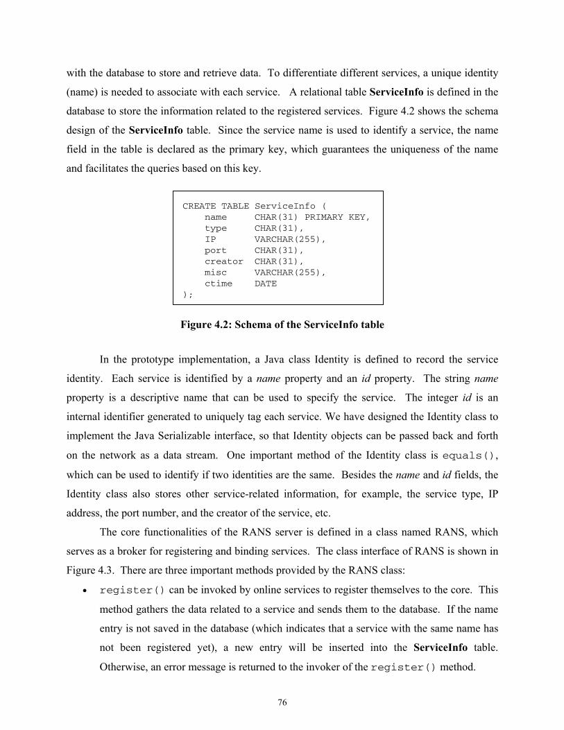
76
with the database to store and retrieve data. To differentiate different services, a unique identity
(name) is needed to associate with each service. A relational table ServiceInfo is defined in the
database to store the information related to the registered services. Figure 4.2 shows the schema
design of the ServiceInfo table. Since the service name is used to identify a service, the name
field in the table is declared as the primary key, which guarantees the uniqueness of the name
and facilitates the queries based on this key.
CREATE TABLE ServiceInfo ( name CHAR(31) PRIMARY KEY, type CHAR(31), IP VARCHAR(255), port CHAR(31), creator CHAR(31), misc VARCHAR(255), ctime DATE );
Figure 4.2: Schema of the ServiceInfo table
In the prototype implementation, a Java class Identity is defined to record the service
identity. Each service is identified by a name property and an id property. The string name
property is a descriptive name that can be used to specify the service. The integer id is an
internal identifier generated to uniquely tag each service. We have designed the Identity class to
implement the Java Serializable interface, so that Identity objects can be passed back and forth
on the network as a data stream. One important method of the Identity class is equals(),
which can be used to identify if two identities are the same. Besides the name and id fields, the
Identity class also stores other service-related information, for example, the service type, IP
address, the port number, and the creator of the service, etc.
The core functionalities of the RANS server is defined in a class named RANS, which
serves as a broker for registering and binding services. The class interface of RANS is shown in
Figure 4.3. There are three important methods provided by the RANS class:
• register() can be invoked by online services to register themselves to the core. This
method gathers the data related to a service and sends them to the database. If the name
entry is not saved in the database (which indicates that a service with the same name has
not been registered yet), a new entry will be inserted into the ServiceInfo table.
Otherwise, an error message is returned to the invoker of the register() method.
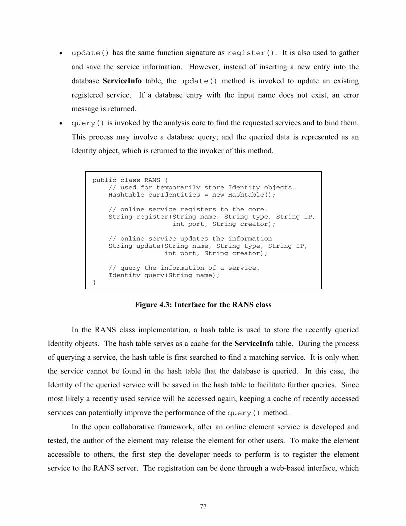
77
• update() has the same function signature as register(). It is also used to gather
and save the service information. However, instead of inserting a new entry into the
database ServiceInfo table, the update() method is invoked to update an existing
registered service. If a database entry with the input name does not exist, an error
message is returned.
• query() is invoked by the analysis core to find the requested services and to bind them.
This process may involve a database query; and the queried data is represented as an
Identity object, which is returned to the invoker of this method.
public class RANS { // used for temporarily store Identity objects. Hashtable curIdentities = new Hashtable(); // online service registers to the core. String register(String name, String type, String IP, int port, String creator); // online service updates the information String update(String name, String type, String IP, int port, String creator); // query the information of a service. Identity query(String name); }
Figure 4.3: Interface for the RANS class
In the RANS class implementation, a hash table is used to store the recently queried
Identity objects. The hash table serves as a cache for the ServiceInfo table. During the process
of querying a service, the hash table is first searched to find a matching service. It is only when
the service cannot be found in the hash table that the database is queried. In this case, the
Identity of the queried service will be saved in the hash table to facilitate further queries. Since
most likely a recently used service will be accessed again, keeping a cache of recently accessed
services can potentially improve the performance of the query() method.
In the open collaborative framework, after an online element service is developed and
tested, the author of the element may release the element for other users. To make the element
accessible to others, the first step the developer needs to perform is to register the element
service to the RANS server. The registration can be done through a web-based interface, which
78
sends the service information to the Java Servlet server, and in turn invokes a certain method of
RANS class.
4.2 DISTRIBUTED ELEMENT SERVICES A key feature of an object-oriented FEA program such as OpenSees is the interchangeability of
components and the ability to integrate existing libraries and new components into the analysis
core without the need to dramatically change the existing code. Introducing a new type of
element into an object-oriented FEA program generally consists of creating a new subclass of
Element class. This local object-computing paradigm can be extended to support distributed
services. Instead of using only the objects that reside exclusively on the local computer, the
collaborative framework also utilizes distributed (remote) objects, which allows the building of a
distributed application to facilitate new element development.
Distributed applications normally comprise two separate programs: a server and a client.
A typical server application creates some remote objects, makes references to them as accessible,
and waits for clients to invoke methods on these remote objects. A typical client application
obtains a remote reference to one or more remote objects in the server and then invokes methods
on them.
4.2.1 Mechanics
The essential requirements in a distributed object system are the ability to create and invoke
objects on a remote host or process, and interact with them as if they were objects within the
same local process. To do so, some kind of message protocol is needed for sending requests to
remote agents to create new objects, to invoke methods on these objects, and to delete the objects
when they are done. Assorted tools and standards for assembling distributed computing
applications have been developed over the years. They started as low-level data transmission
APIs and protocols, such as TCP/IP and RPC (Birrell and Nelson 1984) and have recently begun to
evolve into object-oriented distribution schemes, such as OpenDoc (MacBride et al. 1996),
CORBA (Otte et al. 1996; Pope 1998), DCOM (Eddon and Eddon 1998), and Java RMI (Pitt and
79
McNiff 2001). These programming tools essentially provide a protocol for transmitting structured
data (and, in some case, actual running code) over a network connection.
In the prototype implementation, Java’s Remote Method Invocation (RMI) is chosen to
handle communication for the distributed element services over the Internet. Java RMI enables a
program in one Java Virtual Machine (VM) to make method calls on an object located on a
remote server machine. RMI allows distributing computational tasks across a networked
environment and thus enables a task to be performed on the machine most appropriate for the
task (Farley 1998). The skeleton, which is the object at the server site, receives method
invocation requests from the client. The skeleton then makes a call to the actual object
implemented on the server. The stub is the client’s proxy representing the remote object and
defines all the interfaces that the remote object supports. The RMI architecture defines how
remote objects behave, how and when exceptions can occur, how memory is managed, and how
parameters are communicated with remote methods.
There are many fundamental differences between a local Java object and a remote Java
object, which are summarized in Table 4.1. Because the physical copy of a remote object is
existed in a remote server instead of in the local computer, and is accessed by the clients through
stubs, the behaviors (definition, implementation, creation, and access) of the remote object are
different from a regular local object. In Table 4.1, we also compare the references, finalization,
and exception-handling characteristics between a local object and a remote object. The
references are also called pointers in certain programming languages. The references are like
jumps, which can be used to point to a data structure. If an object is no longer needed by the
system, the object becomes a candidate for finalization, which is a process that the memory and
other computer system resources allocated for the object are reclaimed by the system. Java
automatically reclaims memory used by an object when no object variables refer to that object, a
process known as garbage collection. An exception is an abnormal condition that disrupts
normal program flow. There are many cases where abnormal conditions happen during program
execution, such as the file that the program trying to open may not exist, the network connection
may be disrupted, or a number is divided by zero. If these abnormal conditions are not prevented
or at least handled properly, either the program will be aborted abruptly or incorrect results or
status will be carried on, causing more abnormal conditions. In Java, the exceptions need to be
handled to ensure the correctness and robustness of the program.
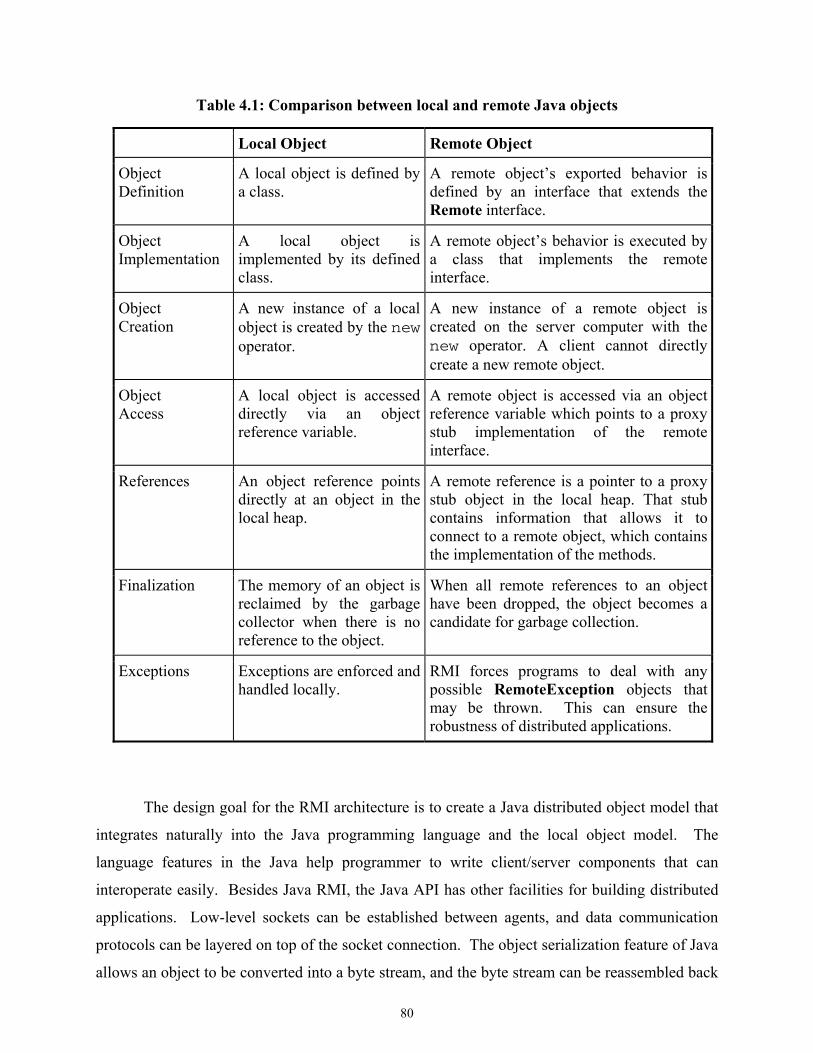
80
Table 4.1: Comparison between local and remote Java objects
Local Object Remote Object
Object Definition
A local object is defined by a class.
A remote object’s exported behavior is defined by an interface that extends the Remote interface.
Object Implementation
A local object is implemented by its defined class.
A remote object’s behavior is executed by a class that implements the remote interface.
Object Creation
A new instance of a local object is created by the new operator.
A new instance of a remote object is created on the server computer with the new operator. A client cannot directly create a new remote object.
Object Access
A local object is accessed directly via an object reference variable.
A remote object is accessed via an object reference variable which points to a proxy stub implementation of the remote interface.
References An object reference points directly at an object in the local heap.
A remote reference is a pointer to a proxy stub object in the local heap. That stub contains information that allows it to connect to a remote object, which contains the implementation of the methods.
Finalization The memory of an object is reclaimed by the garbage collector when there is no reference to the object.
When all remote references to an object have been dropped, the object becomes a candidate for garbage collection.
Exceptions Exceptions are enforced and handled locally.
RMI forces programs to deal with any possible RemoteException objects that may be thrown. This can ensure the robustness of distributed applications.
The design goal for the RMI architecture is to create a Java distributed object model that
integrates naturally into the Java programming language and the local object model. The
language features in the Java help programmer to write client/server components that can
interoperate easily. Besides Java RMI, the Java API has other facilities for building distributed
applications. Low-level sockets can be established between agents, and data communication
protocols can be layered on top of the socket connection. The object serialization feature of Java
allows an object to be converted into a byte stream, and the byte stream can be reassembled back
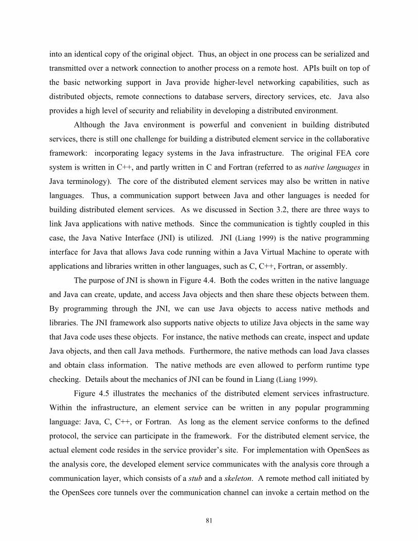
81
into an identical copy of the original object. Thus, an object in one process can be serialized and
transmitted over a network connection to another process on a remote host. APIs built on top of
the basic networking support in Java provide higher-level networking capabilities, such as
distributed objects, remote connections to database servers, directory services, etc. Java also
provides a high level of security and reliability in developing a distributed environment.
Although the Java environment is powerful and convenient in building distributed
services, there is still one challenge for building a distributed element service in the collaborative
framework: incorporating legacy systems in the Java infrastructure. The original FEA core
system is written in C++, and partly written in C and Fortran (referred to as native languages in
Java terminology). The core of the distributed element services may also be written in native
languages. Thus, a communication support between Java and other languages is needed for
building distributed element services. As we discussed in Section 3.2, there are three ways to
link Java applications with native methods. Since the communication is tightly coupled in this
case, the Java Native Interface (JNI) is utilized. JNI (Liang 1999) is the native programming
interface for Java that allows Java code running within a Java Virtual Machine to operate with
applications and libraries written in other languages, such as C, C++, Fortran, or assembly.
The purpose of JNI is shown in Figure 4.4. Both the codes written in the native language
and Java can create, update, and access Java objects and then share these objects between them.
By programming through the JNI, we can use Java objects to access native methods and
libraries. The JNI framework also supports native objects to utilize Java objects in the same way
that Java code uses these objects. For instance, the native methods can create, inspect and update
Java objects, and then call Java methods. Furthermore, the native methods can load Java classes
and obtain class information. The native methods are even allowed to perform runtime type
checking. Details about the mechanics of JNI can be found in Liang (Liang 1999).
Figure 4.5 illustrates the mechanics of the distributed element services infrastructure.
Within the infrastructure, an element service can be written in any popular programming
language: Java, C, C++, or Fortran. As long as the element service conforms to the defined
protocol, the service can participate in the framework. For the distributed element service, the
actual element code resides in the service provider’s site. For implementation with OpenSees as
the analysis core, the developed element service communicates with the analysis core through a
communication layer, which consists of a stub and a skeleton. A remote method call initiated by
the OpenSees core tunnels over the communication channel can invoke a certain method on the
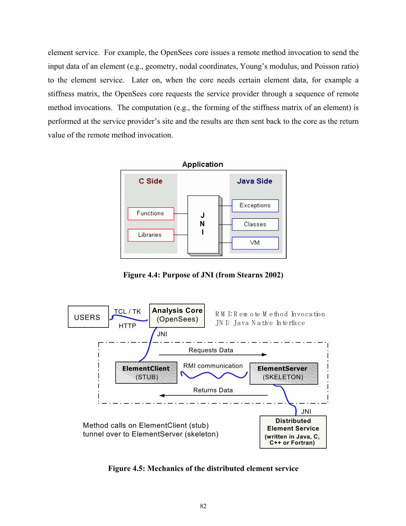
82
element service. For example, the OpenSees core issues a remote method invocation to send the
input data of an element (e.g., geometry, nodal coordinates, Young’s modulus, and Poisson ratio)
to the element service. Later on, when the core needs certain element data, for example a
stiffness matrix, the OpenSees core requests the service provider through a sequence of remote
method invocations. The computation (e.g., the forming of the stiffness matrix of an element) is
performed at the service provider’s site and the results are then sent back to the core as the return
value of the remote method invocation.
Figure 4.4: Purpose of JNI (from Stearns 2002)
USERS
ElementClient(STUB)
ElementServer(SKELETON)
RMI communication
DistributedElement Service
(written in Java, C,C++ or Fortran)
JNI
JNI
Requests Data
Returns Data
Analysis Core(OpenSees)
R M I: R em ote M ethod InvocationJN I: Java N ative InterfaceHTTP
TCL / TK
Method calls on ElementClient (stub)tunnel over to ElementServer (skeleton)
Figure 4.5: Mechanics of the distributed element service
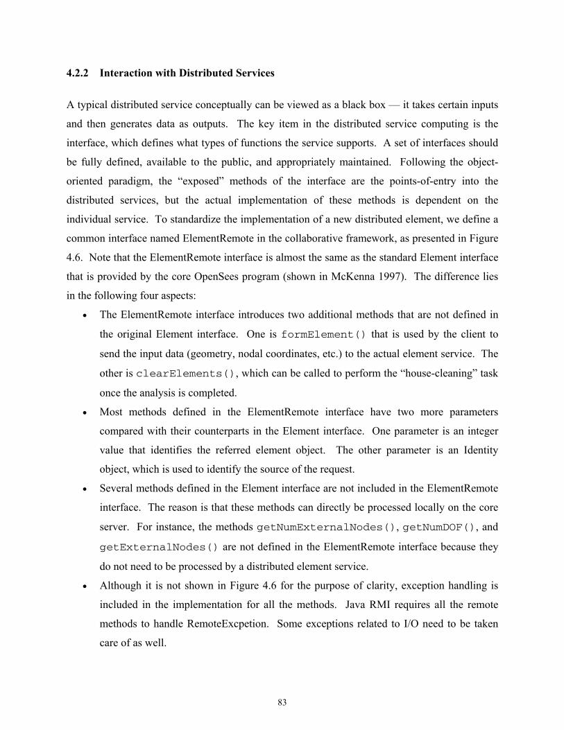
83
4.2.2 Interaction with Distributed Services
A typical distributed service conceptually can be viewed as a black box — it takes certain inputs
and then generates data as outputs. The key item in the distributed service computing is the
interface, which defines what types of functions the service supports. A set of interfaces should
be fully defined, available to the public, and appropriately maintained. Following the object-
oriented paradigm, the “exposed” methods of the interface are the points-of-entry into the
distributed services, but the actual implementation of these methods is dependent on the
individual service. To standardize the implementation of a new distributed element, we define a
common interface named ElementRemote in the collaborative framework, as presented in Figure
4.6. Note that the ElementRemote interface is almost the same as the standard Element interface
that is provided by the core OpenSees program (shown in McKenna 1997). The difference lies
in the following four aspects:
• The ElementRemote interface introduces two additional methods that are not defined in
the original Element interface. One is formElement() that is used by the client to
send the input data (geometry, nodal coordinates, etc.) to the actual element service. The
other is clearElements(), which can be called to perform the “house-cleaning” task
once the analysis is completed.
• Most methods defined in the ElementRemote interface have two more parameters
compared with their counterparts in the Element interface. One parameter is an integer
value that identifies the referred element object. The other parameter is an Identity
object, which is used to identify the source of the request.
• Several methods defined in the Element interface are not included in the ElementRemote
interface. The reason is that these methods can directly be processed locally on the core
server. For instance, the methods getNumExternalNodes(), getNumDOF(), and
getExternalNodes() are not defined in the ElementRemote interface because they
do not need to be processed by a distributed element service.
• Although it is not shown in Figure 4.6 for the purpose of clarity, exception handling is
included in the implementation for all the methods. Java RMI requires all the remote
methods to handle RemoteExcpetion. Some exceptions related to I/O need to be taken
care of as well.
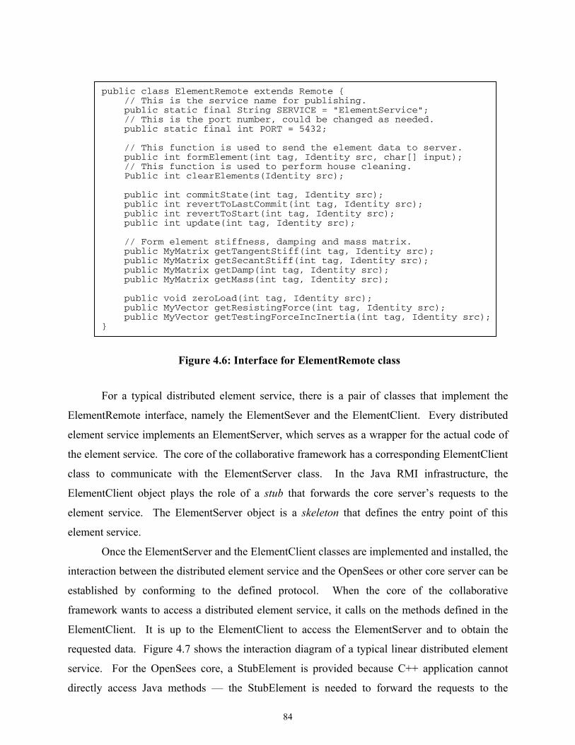
84
public class ElementRemote extends Remote { // This is the service name for publishing. public static final String SERVICE = "ElementService"; // This is the port number, could be changed as needed. public static final int PORT = 5432; // This function is used to send the element data to server. public int formElement(int tag, Identity src, char[] input); // This function is used to perform house cleaning. Public int clearElements(Identity src); public int commitState(int tag, Identity src); public int revertToLastCommit(int tag, Identity src); public int revertToStart(int tag, Identity src); public int update(int tag, Identity src); // Form element stiffness, damping and mass matrix. public MyMatrix getTangentStiff(int tag, Identity src); public MyMatrix getSecantStiff(int tag, Identity src); public MyMatrix getDamp(int tag, Identity src); public MyMatrix getMass(int tag, Identity src); public void zeroLoad(int tag, Identity src); public MyVector getResistingForce(int tag, Identity src); public MyVector getTestingForceIncInertia(int tag, Identity src); }
Figure 4.6: Interface for ElementRemote class
For a typical distributed element service, there is a pair of classes that implement the
ElementRemote interface, namely the ElementSever and the ElementClient. Every distributed
element service implements an ElementServer, which serves as a wrapper for the actual code of
the element service. The core of the collaborative framework has a corresponding ElementClient
class to communicate with the ElementServer class. In the Java RMI infrastructure, the
ElementClient object plays the role of a stub that forwards the core server’s requests to the
element service. The ElementServer object is a skeleton that defines the entry point of this
element service.
Once the ElementServer and the ElementClient classes are implemented and installed, the
interaction between the distributed element service and the OpenSees or other core server can be
established by conforming to the defined protocol. When the core of the collaborative
framework wants to access a distributed element service, it calls on the methods defined in the
ElementClient. It is up to the ElementClient to access the ElementServer and to obtain the
requested data. Figure 4.7 shows the interaction diagram of a typical linear distributed element
service. For the OpenSees core, a StubElement is provided because C++ application cannot
directly access Java methods — the StubElement is needed to forward the requests to the
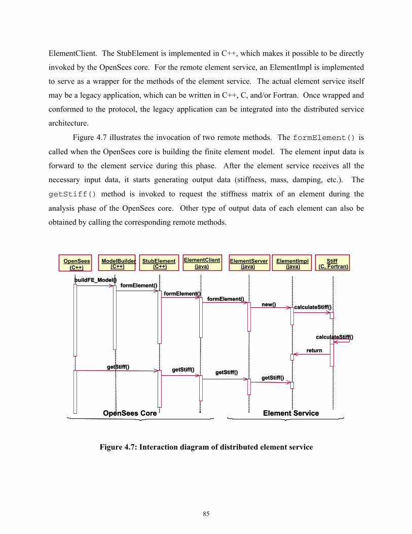
85
ElementClient. The StubElement is implemented in C++, which makes it possible to be directly
invoked by the OpenSees core. For the remote element service, an ElementImpl is implemented
to serve as a wrapper for the methods of the element service. The actual element service itself
may be a legacy application, which can be written in C++, C, and/or Fortran. Once wrapped and
conformed to the protocol, the legacy application can be integrated into the distributed service
architecture.
Figure 4.7 illustrates the invocation of two remote methods. The formElement() is
called when the OpenSees core is building the finite element model. The element input data is
forward to the element service during this phase. After the element service receives all the
necessary input data, it starts generating output data (stiffness, mass, damping, etc.). The
getStiff() method is invoked to request the stiffness matrix of an element during the
analysis phase of the OpenSees core. Other type of output data of each element can also be
obtained by calling the corresponding remote methods.
ModelBuilder
(C++)ElementServer
(java)ElementImpl
(java)Stiff
(C, Fortran)ElementClient
(java)StubElement
(C++)OpenSees
(C++)
buildFE_Model()formElement()
formElement()formElement()
new() calculateStiff()
calculateStiff()
getStiff() getStiff() getStiff()
return
getStiff()
OpenSees Core Element Service
ModelBuilder(C++)
ElementServer(java)
ElementImpl(java)
Stiff(C, Fortran)
ElementClient(java)
StubElement(C++)
OpenSees(C++)
buildFE_Model()formElement()
formElement()formElement()
new() calculateStiff()
calculateStiff()
getStiff() getStiff() getStiff()
return
getStiff()
OpenSees Core Element Service
Figure 4.7: Interaction diagram of distributed element service
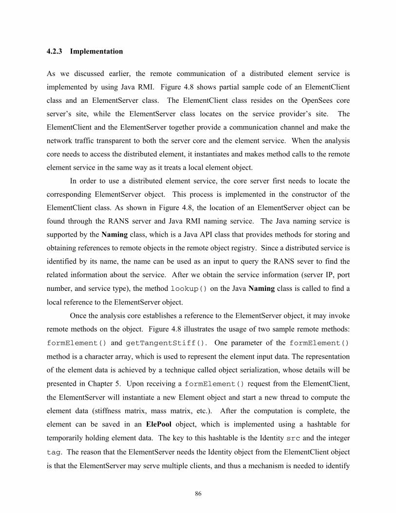
86
4.2.3 Implementation
As we discussed earlier, the remote communication of a distributed element service is
implemented by using Java RMI. Figure 4.8 shows partial sample code of an ElementClient
class and an ElementServer class. The ElementClient class resides on the OpenSees core
server’s site, while the ElementServer class locates on the service provider’s site. The
ElementClient and the ElementServer together provide a communication channel and make the
network traffic transparent to both the server core and the element service. When the analysis
core needs to access the distributed element, it instantiates and makes method calls to the remote
element service in the same way as it treats a local element object.
In order to use a distributed element service, the core server first needs to locate the
corresponding ElementServer object. This process is implemented in the constructor of the
ElementClient class. As shown in Figure 4.8, the location of an ElementServer object can be
found through the RANS server and Java RMI naming service. The Java naming service is
supported by the Naming class, which is a Java API class that provides methods for storing and
obtaining references to remote objects in the remote object registry. Since a distributed service is
identified by its name, the name can be used as an input to query the RANS sever to find the
related information about the service. After we obtain the service information (server IP, port
number, and service type), the method lookup() on the Java Naming class is called to find a
local reference to the ElementServer object.
Once the analysis core establishes a reference to the ElementServer object, it may invoke
remote methods on the object. Figure 4.8 illustrates the usage of two sample remote methods:
formElement() and getTangentStiff(). One parameter of the formElement()
method is a character array, which is used to represent the element input data. The representation
of the element data is achieved by a technique called object serialization, whose details will be
presented in Chapter 5. Upon receiving a formElement() request from the ElementClient,
the ElementServer will instantiate a new Element object and start a new thread to compute the
element data (stiffness matrix, mass matrix, etc.). After the computation is complete, the
element can be saved in an ElePool object, which is implemented using a hashtable for
temporarily holding element data. The key to this hashtable is the Identity src and the integer
tag. The reason that the ElementServer needs the Identity object from the ElementClient object
is that the ElementServer may serve multiple clients, and thus a mechanism is needed to identify
87
the source of the remote requests. During a structural analysis, when the OpenSees core needs
the stiffness matrix, it issues a call getTangentStiff() to ElementServer for the stiffness
matrix. At this stage, the ElePool object is searched for by the requested Element object and the
stiffness matrix can be sent to the ElementClient as return of the function.
public class ElementClient { // based on the server name and port number, creates stub object. public ElementClient(String serverName) { Identity server = theRANS.query(serverName); System.setSecurityManager(new RMISecurityManager()); String name = "//" + server.IP + ":" + server.PORT + "/" + server.SERVICE; theStub = (ElementRemote)Naming.lookup(name); } // the stub is a proxy to the real server object. public void formElement(int tag, Identity src, char[] input) { theStub.formElement(tag, src, input); } public MyMatrix getTangentStiff(int tag, Identity src) { MyMatrix result = new MyMatrix(4, 4); result = theStub.getTangentStiff(tag, src); return result; } } public class ElementServer extends UnicastRemoteObject implements ElementRemote { // the ElePool provides functions similar to that of a hashtable. private ElePool allElements = new ElePool(); public void formElement(int tag, Identity src, char[] input) { ElementImpl newElement = new ElementImpl(tag, input); allElements.put(tag, src, newElement); } public MyMatrix getTangentStiff(String tag, Identity src) { ElementImpl oneElement=(ElementImpl)allElements.get(tag, src); result = oneElement.getTangentStiff(); return result; } }
Figure 4.8: Sample ElementClient and sample ElementServer
88
After the communication is initiated, the core analysis program treats the distributed
element in the same way as a local element. Again, the searching and the binding of an online
remote element service are automated — the user of the collaborative framework is not aware of
the difference between a local element and an online element.
4.3 DYNAMIC SHARED LIBRARY ELEMENT SERVICES
The distributed element service model described in the previous section is flexible and
convenient. However, the approach does carry some overhead on remote method invocation,
which is generally more expensive than local method call. The system performance is reduced
because a remote method has to be invoked for accessing every distributed element. A dynamic
shared library (or simply a shared library) element service is designed to alleviate the
performance bottleneck and to improve the system performance without losing the flexibility and
other benefits of the distributed services. Instead of being compiled to a static library and
merged to the core server, an element service is built as a dynamic shared library and located on
the element service provider’s site. During the system runtime, the installed shared library can
be automatically downloaded to the core server and linked with the OpenSees core. The shared
library element service allows the replacement of an element service without reinitiating the core
server, as well as provides a transparent service to the users.
4.3.1 Static Library vs. Shared Library
Most modern operating systems allow us to create and use two kinds of libraries — static
libraries and shared libraries. A dynamic shared library differs in many ways from a static
library. Static libraries are just collections of object files that are linked into the program during
the linking phase of compilation, and are not relevant during runtime. Only those object files
from the library that are needed by the application are linked into the executable program.
Shared libraries, on the other hand, are linked into the program in two stages. First, during
compilation time, the linker verifies that all the symbols (functions, variables, and the like)
required by the program are either linked into the program or existed in one of its shared
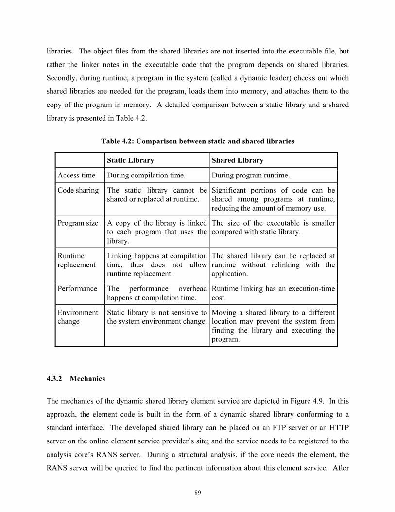
89
libraries. The object files from the shared libraries are not inserted into the executable file, but
rather the linker notes in the executable code that the program depends on shared libraries.
Secondly, during runtime, a program in the system (called a dynamic loader) checks out which
shared libraries are needed for the program, loads them into memory, and attaches them to the
copy of the program in memory. A detailed comparison between a static library and a shared
library is presented in Table 4.2.
Table 4.2: Comparison between static and shared libraries
Static Library Shared Library
Access time During compilation time. During program runtime.
Code sharing The static library cannot be shared or replaced at runtime.
Significant portions of code can be shared among programs at runtime, reducing the amount of memory use.
Program size A copy of the library is linked to each program that uses the library.
The size of the executable is smaller compared with static library.
Runtime replacement
Linking happens at compilation time, thus does not allow runtime replacement.
The shared library can be replaced at runtime without relinking with the application.
Performance The performance overhead happens at compilation time.
Runtime linking has an execution-time cost.
Environment change
Static library is not sensitive to the system environment change.
Moving a shared library to a different location may prevent the system from finding the library and executing the program.
4.3.2 Mechanics
The mechanics of the dynamic shared library element service are depicted in Figure 4.9. In this
approach, the element code is built in the form of a dynamic shared library conforming to a
standard interface. The developed shared library can be placed on an FTP server or an HTTP
server on the online element service provider’s site; and the service needs to be registered to the
analysis core’s RANS server. During a structural analysis, if the core needs the element, the
RANS server will be queried to find the pertinent information about this element service. After
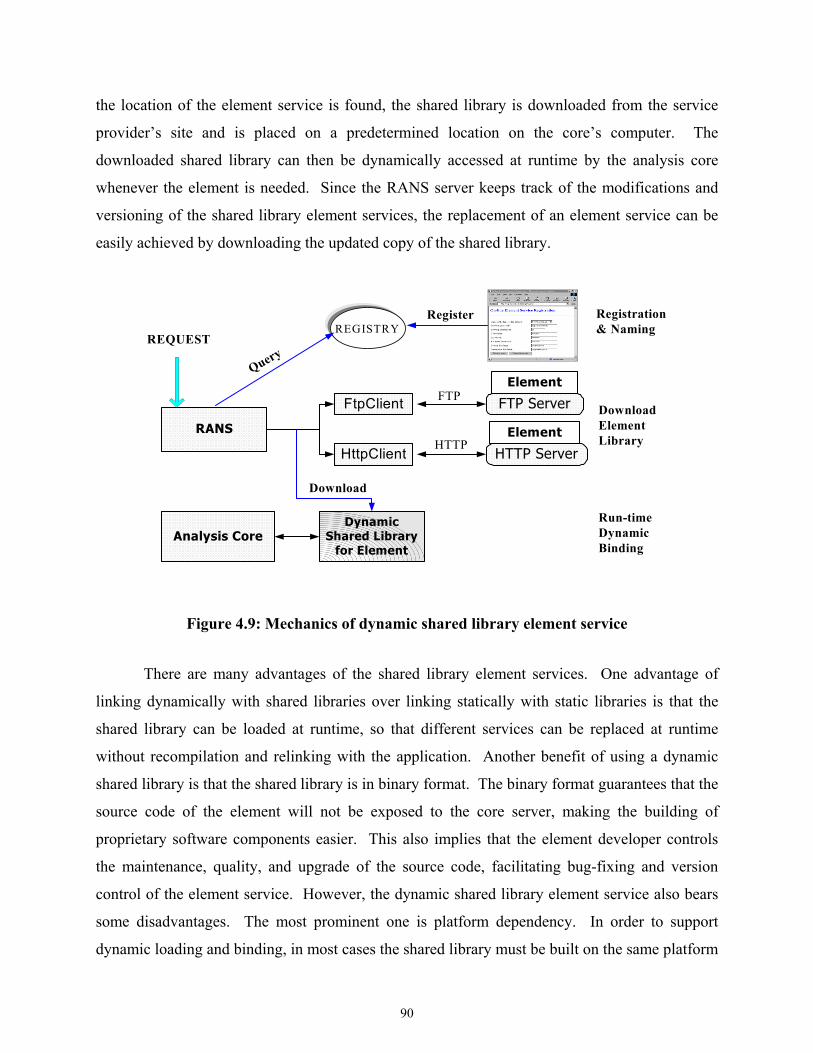
90
the location of the element service is found, the shared library is downloaded from the service
provider’s site and is placed on a predetermined location on the core’s computer. The
downloaded shared library can then be dynamically accessed at runtime by the analysis core
whenever the element is needed. Since the RANS server keeps track of the modifications and
versioning of the shared library element services, the replacement of an element service can be
easily achieved by downloading the updated copy of the shared library.
FTP Server
HTTP Server
REGISTRY
FtpClient
HttpClient
RANS
DynamicShared Library
for Element
Element
Element
Analysis Core
Register Registration& Naming
DownloadElementLibrary
Run-timeDynamicBinding
FTP
HTTP
REQUEST
Query
Download
Figure 4.9: Mechanics of dynamic shared library element service
There are many advantages of the shared library element services. One advantage of
linking dynamically with shared libraries over linking statically with static libraries is that the
shared library can be loaded at runtime, so that different services can be replaced at runtime
without recompilation and relinking with the application. Another benefit of using a dynamic
shared library is that the shared library is in binary format. The binary format guarantees that the
source code of the element will not be exposed to the core server, making the building of
proprietary software components easier. This also implies that the element developer controls
the maintenance, quality, and upgrade of the source code, facilitating bug-fixing and version
control of the element service. However, the dynamic shared library element service also bears
some disadvantages. The most prominent one is platform dependency. In order to support
dynamic loading and binding, in most cases the shared library must be built on the same platform
91
as the core server. Other disadvantages include potential security problems and minor
performance overhead due to network downloading and dynamic binding.
4.3.3 Implementation
There are three issues associated with the implementation of the dynamic shared library element
service. The first is about how to build a shared library; the second is related to the downloading
of shared library services; and the third is regarding the dynamic binding of a shared element
library.
We first address the issue of how to build a dynamic shared library. As we mentioned
earlier, the building of a dynamic shared library is platform dependent. The dynamic shared
libraries are supported and implemented on various operating systems:
• Windows: In the Windows platform, shared libraries are called “dynamic link libraries”
(DLLs) (Microsoft-Corporation. 2002) and a DLL file is often given the .dll file name
suffix. DLLs are primarily controlled by three functions: LoadLibrary(),
GetProcAddress(), and FreeLibrary(). The Win32 API function
LoadLibrary() is used to load a DLL into the caller’s address space.
GetProcAddress() is used to retrieve pointers to the DLL’s exported functions so
that the client can call those functions in the DLL. When a client has finished using the
library, the DLL is freed by calling FreeLibrary(). The Microsoft Visual C++
compiler can be used to compile DLLs and the programs that load them.
• Linux: For the Linux platform, the dlopen family of routines is used to control the
shared libraries (Norton 2000). The library should be named with a .so file name suffix.
In order to find the location of a library, Linux searches along the LD_LIBRARY_PATH
environment variable, which is a colon-separated list of directories. The directories listed
in /etc/lod.so.cache file and the directories /usr/lib and /lib will also be
searched. The GNU C compiler (gcc and g++) can be used to compile shared libraries or
programs that load them.
• SunOS: The shared libraries in the SunOS are very similar to that in the Linux
environment. A shared library is loaded using the method dlopen(), the functions of a
shared library is called using dlsym(), and the shared library is unloaded using
92
dlclose(). The Sun Workshop (Sun-Microsystems 2001) compiler (CC and cc) can be
used to compile shared libraries and programs that load them.
In the prototype implementation of the collaborative framework, Sun workstations are
used as the development platform. For illustration purpose, we will focus on building dynamic
shared libraries in the SunOS environment. The shared library element services on other
platforms can be constructed similarly. In the SunOS environment, the creation of a shared
library is quite similar to the creation of a static library — compile a list of object files and then
insert them into a library file. However, there are two major differences:
1. Compile for Position Independent Code (PIC). When the object files are generated, the
positions in a program that these files will be inserted into are unknown. Thus, all the
subroutine calls in the shared library need to use relative addresses, instead of absolute
addresses. We can use the compilation flag ‘-fPIC’ to generate this type of code.
2. Library File Creation. Unlike a static library, a shared library is not an archive file. We
need to tell the compiler to create a shared library instead of a final program executable
file. This can be achieved by using the ‘–shared’ flag with the Sun compiler.
Thus, the set of commands we may use to create a shared library would be as follows:
cc –fPIC –c util_file.c
cc –fPIC –c element1.c
cc –shared libele1.so util_file.o element1.o
The first two commands compile the source files with the -fPIC option, so that they will
be suitable for use in a shared library. The last command asks the compiler to generate a shared
library named libele1.so.
After a shared library element service is implemented and tested on the service
developer’s site, the next problem is how to automatically download the library to the analysis
core server. This task can be achieved by utilizing one of the two popular Internet protocols
(FTP and HTTP) to transfer the library files. On the element service developer’s site, the
developed shared element libraries are placed on either an FTP server or a web server. The
location of the shared library and other pertinent information can be submitted to the core server
via the RANS interface. On the analysis core server’s site, two new classes, namely FtpClient
and HttpClient, are implemented. These two classes can query the RANS server for the related
information of a particular element service, and then use queried results to find the element
libraries and to download the library files from the element developer’s site. The downloaded
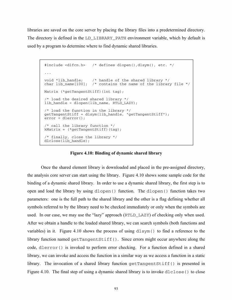
93
libraries are saved on the core server by placing the library files into a predetermined directory.
The directory is defined in the LD_LIBRARY_PATH environment variable, which by default is
used by a program to determine where to find dynamic shared libraries.
#include <dlfcn.h> /* defines dlopen(),dlsym(), etc. */ ... void *lib_handle; /* handle of the shared library */ char lib_name[100]; /* contains the name of the library file */ Matrix (*getTangentStiff)(int tag); /* load the desired shared library */ lib_handle = dlopen(lib_name, RTLD_LAZY); /* load the function in the library */ getTangentStiff = dlsym(lib_handle, "getTangentStiff"); error = dlerror(); /* call the library function */ kMatrix = (*getTangentStiff)(tag); /* finally, close the library */ dlclose(lib_handle);
Figure 4.10: Binding of dynamic shared library
Once the shared element library is downloaded and placed in the pre-assigned directory,
the analysis core server can start using the library. Figure 4.10 shows some sample code for the
binding of a dynamic shared library. In order to use a dynamic shared library, the first step is to
open and load the library by using dlopen() function. The dlopen() function takes two
parameters: one is the full path to the shared library and the other is a flag defining whether all
symbols referred to by the library need to be checked immediately or only when the symbols are
used. In our case, we may use the “lazy” approach (RTLD_LAZY) of checking only when used.
After we obtain a handle to the loaded shared library, we can search symbols (both functions and
variables) in it. Figure 4.10 shows the process of using dlsym() to find a reference to the
library function named getTangentStiff(). Since errors might occur anywhere along the
code, dlerror() is invoked to perform error checking. For a function defined in a shared
library, we can invoke and access the function in a similar way as we access a function in a static
library. The invocation of a shared library function getTangentStiff() is presented in
Figure 4.10. The final step of using a dynamic shared library is to invoke dlclose() to close
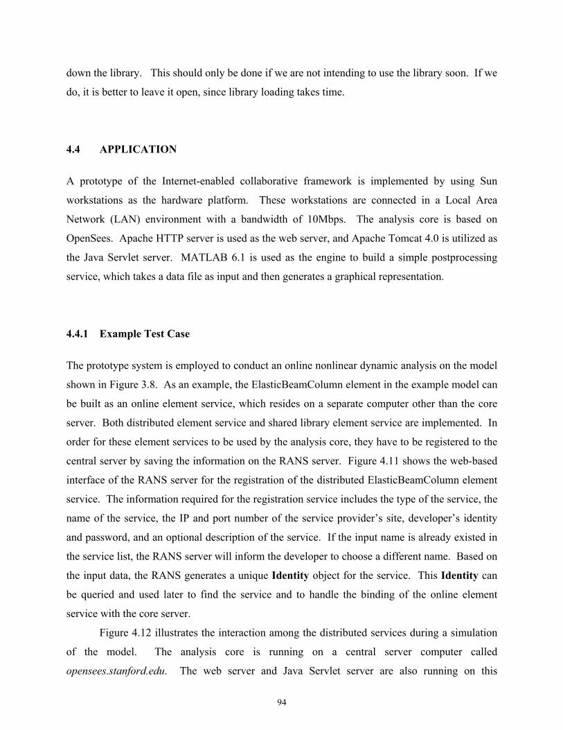
94
down the library. This should only be done if we are not intending to use the library soon. If we
do, it is better to leave it open, since library loading takes time.
4.4 APPLICATION
A prototype of the Internet-enabled collaborative framework is implemented by using Sun
workstations as the hardware platform. These workstations are connected in a Local Area
Network (LAN) environment with a bandwidth of 10Mbps. The analysis core is based on
OpenSees. Apache HTTP server is used as the web server, and Apache Tomcat 4.0 is utilized as
the Java Servlet server. MATLAB 6.1 is used as the engine to build a simple postprocessing
service, which takes a data file as input and then generates a graphical representation.
4.4.1 Example Test Case
The prototype system is employed to conduct an online nonlinear dynamic analysis on the model
shown in Figure 3.8. As an example, the ElasticBeamColumn element in the example model can
be built as an online element service, which resides on a separate computer other than the core
server. Both distributed element service and shared library element service are implemented. In
order for these element services to be used by the analysis core, they have to be registered to the
central server by saving the information on the RANS server. Figure 4.11 shows the web-based
interface of the RANS server for the registration of the distributed ElasticBeamColumn element
service. The information required for the registration service includes the type of the service, the
name of the service, the IP and port number of the service provider’s site, developer’s identity
and password, and an optional description of the service. If the input name is already existed in
the service list, the RANS server will inform the developer to choose a different name. Based on
the input data, the RANS generates a unique Identity object for the service. This Identity can
be queried and used later to find the service and to handle the binding of the online element
service with the core server.
Figure 4.12 illustrates the interaction among the distributed services during a simulation
of the model. The analysis core is running on a central server computer called
opensees.stanford.edu. The web server and Java Servlet server are also running on this
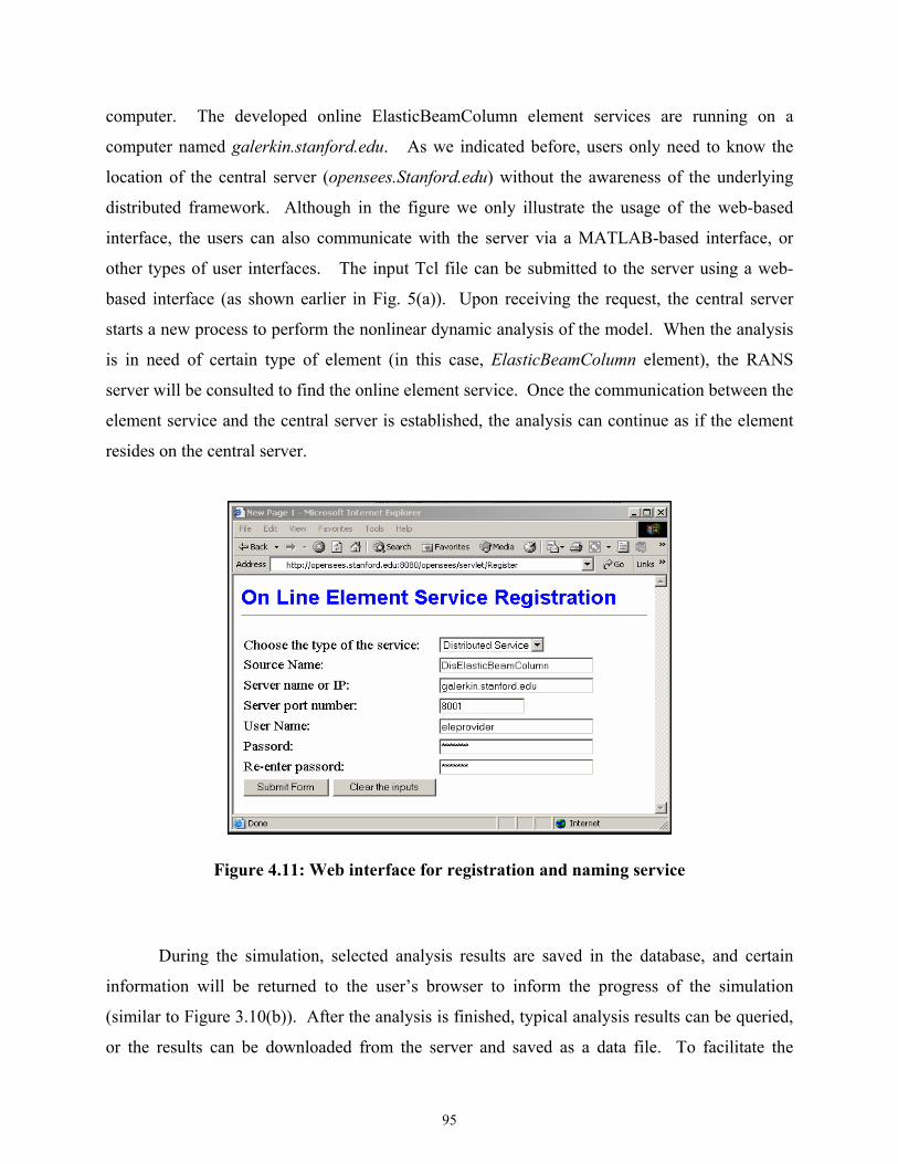
95
computer. The developed online ElasticBeamColumn element services are running on a
computer named galerkin.stanford.edu. As we indicated before, users only need to know the
location of the central server (opensees.Stanford.edu) without the awareness of the underlying
distributed framework. Although in the figure we only illustrate the usage of the web-based
interface, the users can also communicate with the server via a MATLAB-based interface, or
other types of user interfaces. The input Tcl file can be submitted to the server using a web-
based interface (as shown earlier in Fig. 5(a)). Upon receiving the request, the central server
starts a new process to perform the nonlinear dynamic analysis of the model. When the analysis
is in need of certain type of element (in this case, ElasticBeamColumn element), the RANS
server will be consulted to find the online element service. Once the communication between the
element service and the central server is established, the analysis can continue as if the element
resides on the central server.
Figure 4.11: Web interface for registration and naming service
During the simulation, selected analysis results are saved in the database, and certain
information will be returned to the user’s browser to inform the progress of the simulation
(similar to Figure 3.10(b)). After the analysis is finished, typical analysis results can be queried,
or the results can be downloaded from the server and saved as a data file. To facilitate the
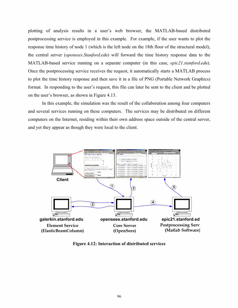
96
plotting of analysis results in a user’s web browser, the MATLAB-based distributed
postprocessing service is employed in this example. For example, if the user wants to plot the
response time history of node 1 (which is the left node on the 18th floor of the structural model),
the central server (opensees.Stanford.edu) will forward the time history response data to the
MATLAB-based service running on a separate computer (in this case, epic21.stanford.edu).
Once the postprocessing service receives the request, it automatically starts a MATLAB process
to plot the time history response and then save it in a file of PNG (Portable Network Graphics)
format. In responding to the user’s request, this file can later be sent to the client and be plotted
on the user’s browser, as shown in Figure 4.13.
In this example, the simulation was the result of the collaboration among four computers
and several services running on these computers. The services may be distributed on different
computers on the Internet, residing within their own address space outside of the central server,
and yet they appear as though they were local to the client.
opensees.stanford.edu epic21.stanford.edugalerkin.stanford.eduElement Service
(ElasticBeamColumn)Postprocessing Servi
(Matlab Software)Core Server(OpenSees)
Client1 3
2 4
5
Figure 4.12: Interaction of distributed services
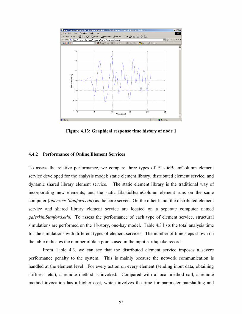
97
Figure 4.13: Graphical response time history of node 1
4.4.2 Performance of Online Element Services
To assess the relative performance, we compare three types of ElasticBeamColumn element
service developed for the analysis model: static element library, distributed element service, and
dynamic shared library element service. The static element library is the traditional way of
incorporating new elements, and the static ElasticBeamColumn element runs on the same
computer (opensees.Stanford.edu) as the core server. On the other hand, the distributed element
service and shared library element service are located on a separate computer named
galerkin.Stanford.edu. To assess the performance of each type of element service, structural
simulations are performed on the 18-story, one-bay model. Table 4.3 lists the total analysis time
for the simulations with different types of element services. The number of time steps shown on
the table indicates the number of data points used in the input earthquake record.
From Table 4.3, we can see that the distributed element service imposes a severe
performance penalty to the system. This is mainly because the network communication is
handled at the element level. For every action on every element (sending input data, obtaining
stiffness, etc.), a remote method is invoked. Compared with a local method call, a remote
method invocation has a higher cost, which involves the time for parameter marshalling and
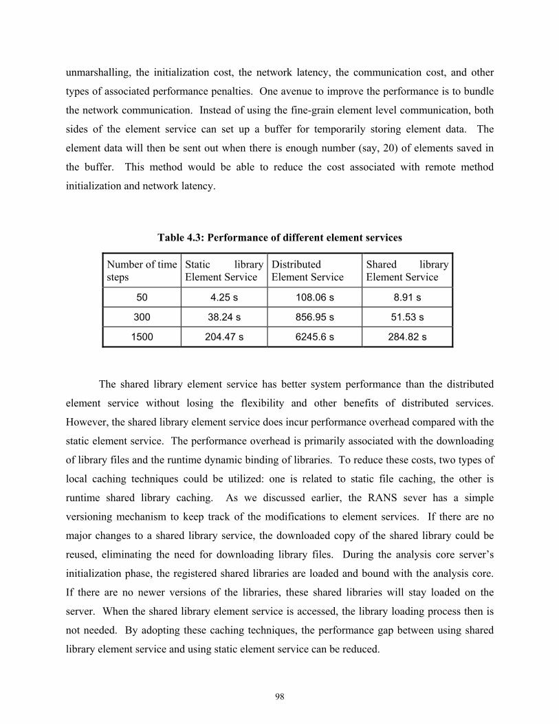
98
unmarshalling, the initialization cost, the network latency, the communication cost, and other
types of associated performance penalties. One avenue to improve the performance is to bundle
the network communication. Instead of using the fine-grain element level communication, both
sides of the element service can set up a buffer for temporarily storing element data. The
element data will then be sent out when there is enough number (say, 20) of elements saved in
the buffer. This method would be able to reduce the cost associated with remote method
initialization and network latency.
Table 4.3: Performance of different element services
Number of time steps
Static library Element Service
Distributed Element Service
Shared library Element Service
50 4.25 s 108.06 s 8.91 s
300 38.24 s 856.95 s 51.53 s
1500 204.47 s 6245.6 s 284.82 s
The shared library element service has better system performance than the distributed
element service without losing the flexibility and other benefits of distributed services.
However, the shared library element service does incur performance overhead compared with the
static element service. The performance overhead is primarily associated with the downloading
of library files and the runtime dynamic binding of libraries. To reduce these costs, two types of
local caching techniques could be utilized: one is related to static file caching, the other is
runtime shared library caching. As we discussed earlier, the RANS sever has a simple
versioning mechanism to keep track of the modifications to element services. If there are no
major changes to a shared library service, the downloaded copy of the shared library could be
reused, eliminating the need for downloading library files. During the analysis core server’s
initialization phase, the registered shared libraries are loaded and bound with the analysis core.
If there are no newer versions of the libraries, these shared libraries will stay loaded on the
server. When the shared library element service is accessed, the library loading process then is
not needed. By adopting these caching techniques, the performance gap between using shared
library element service and using static element service can be reduced.
99
4.5 SUMMARY AND DISCUSSION The collaborative framework as discussed in the previous chapter consists of six distinct
modules, and this chapter describes three of them, namely the registration and naming service,
the distributed element service, and the dynamic shared library element service. The RANS
sever allows the analysis core to find the registered services and to monitor the modifications to
these services. Since RANS guarantees that a unique name is associated with each service, the
name can be used to query and identify a service. The distributed element service and dynamic
shared library element service are two forms of online element services, which are introduced to
the core framework to facilitate the distributed usage and the collaborative development of an
finite element structural analysis program. An element service may be developed as a
component that can be easily integrated with the core server through a plug-and-play
environment.
The collaborative framework has multiple benefits, within which two prominent ones are
standardized interface and network transparency. An online service is best defined in terms of
the protocol it uses, rather than particular software participated in the system. Any
implementation of these protocols is able to participate in the system, interoperating with
completely independent implementations, but using the same protocols. The standard
communication protocols allow a service to be replaced easily and facilitate the concurrent
development of standardized components. The collaborative framework system provides an
execution environment that is network transparent. Being network transparent means the
execution environment provides an abstraction that is the same whether executing locally,
remotely, or distributively — the network is not visible. End users of the collaborative
framework do not need to be aware of the complexity of the core server (in terms of both
hardware and software infrastructure), hence they do not have the associated development and
maintenance challenges.
The collaborative framework with online services described in this chapter does not
address issues of authentication and security. The security issues could be addressed at the
network level, especially by utilizing the Public Key Infrastructure (PKI) that supports digital
signatures and other public key-enabled security services (Stallings 1998). One example of
managing security for high-performance distributed computing is the security architecture
(Foster et al. 1998) used for Computational Grid (Foster et al. 2001), where the integrity and
confidentiality of communications are ensured. Another issue of the collaborative framework is

100
scalability. The current implementation relies on Java’s multithreading feature to handle
simultaneous requests. Our test result shows that the performance will be substantially degraded
when more than a dozen clients access the server simultaneously. This scalability problem could
be tackled by providing multiple core servers, utilizing more powerful computers, and deploying
parallel and distributed computing environments (De-Santiago and Law 2000; Mackay and Law
1996).
5 Data Access and Project Management
The importance of engineering data management is increasingly emphasized in both industrial
and academic communities. The objective of using an engineering database is to provide the
users the needed engineering information from readily accessible sources in a ready-to-use
format for further manipulation. Such a trend can also be observed in the field of finite element
analysis. Modern finite element programs are increasingly required to be linked to other
software such as CAD, graphical processing software, or databases (Mackie 1997). Data
integration problems are mounting as engineers confront the need to move information from one
computer program to another in a reliable and organized manner. The handling of data shared
between disparate systems requires the definition of persistent and standard representations of
the data, and corresponding interfaces to query the data. Data must be represented in such a
manner to facilitate interoperation with people or mechanisms that use other persistent
representations (van-Engelen et al. 2000).
This chapter presents a prototype implementation of an online data access system for the
open collaborative software framework (Peng 2002). In this work, a COTS database system is
linked with the central server to provide the persistent storage of selected analysis results. By
adopting a COTS database system, we can address many of the problems encountered by the
prevailing file system-based data management. Current trends indicate that the commercial
database industry is shifting to use the Internet as the preferred data delivery vehicle. Various
Internet computing is supported by backend databases. Finite element computing is no
exception. The online data access system would allow the users to query the core server for
useful analysis results, and the information retrieved from the database through the core server is
returned to the users in a standard format. Since the system is using a centralized server model,
the data management system can also support project management and version control of the
projects.
102
This chapter is organized as follows:
• Section 5.1 presents the multi-tiered architecture of the online data access system. The
communications between different tiers are discussed.
• The data storage scheme is presented in Section 5.2. A selective data storage scheme is
introduced to provide flexible support for the tradeoff between the time used for
reconstructing an analysis domain and the space used for storing the analysis results.
• Section 5.3 describes the data representations of the online data access system. Both
internal and external data representations are described.
• Section 5.4 discusses several issues regarding data query and retrieval. A data query
language is introduced in this section, and the data query interfaces are presented.
• Section 5.5 presents two test case examples for the usage of the data access and project
management system. The benefits of using the proposed data access system are
discussed in this section.
5.1 MULTITIERED ARCHITECTURE As shown in Figure 3.3, the online data access system is designed as one module of the Internet-
enabled collaborative framework to provide researchers and engineers with easy and efficient
access to the structural analysis results. During an analysis, certain selected results and pertinent
data are saved, and a data storage and access system is employed to manage these data.
To design a data management system, we first need to decide what kind of media should
be used to store the data. Presently, the data storage for finite element analysis programs
primarily relies on file systems. Since most modern operating systems have built-in support for
file usage, directly using file systems to store data is a straightforward process. However, there
are many intrinsic drawbacks associated with the direct usage of file system for storing large
volume of data. File systems generally do not guarantee that data cannot be lost if the data are
not backed up, and they do not support efficient random access in which case the locations of
data items in a particular file are unknown. Furthermore, file systems do not provide direct
support for a query language to access the data in files, and their support for a schema of the data
is limited to the creation of file directory structures. Finally, file systems cannot guarantee data
integrity in the case of concurrent access. Instead of directly using the file systems to store the
analysis results of a finite element analysis, these results can also be saved in database systems.
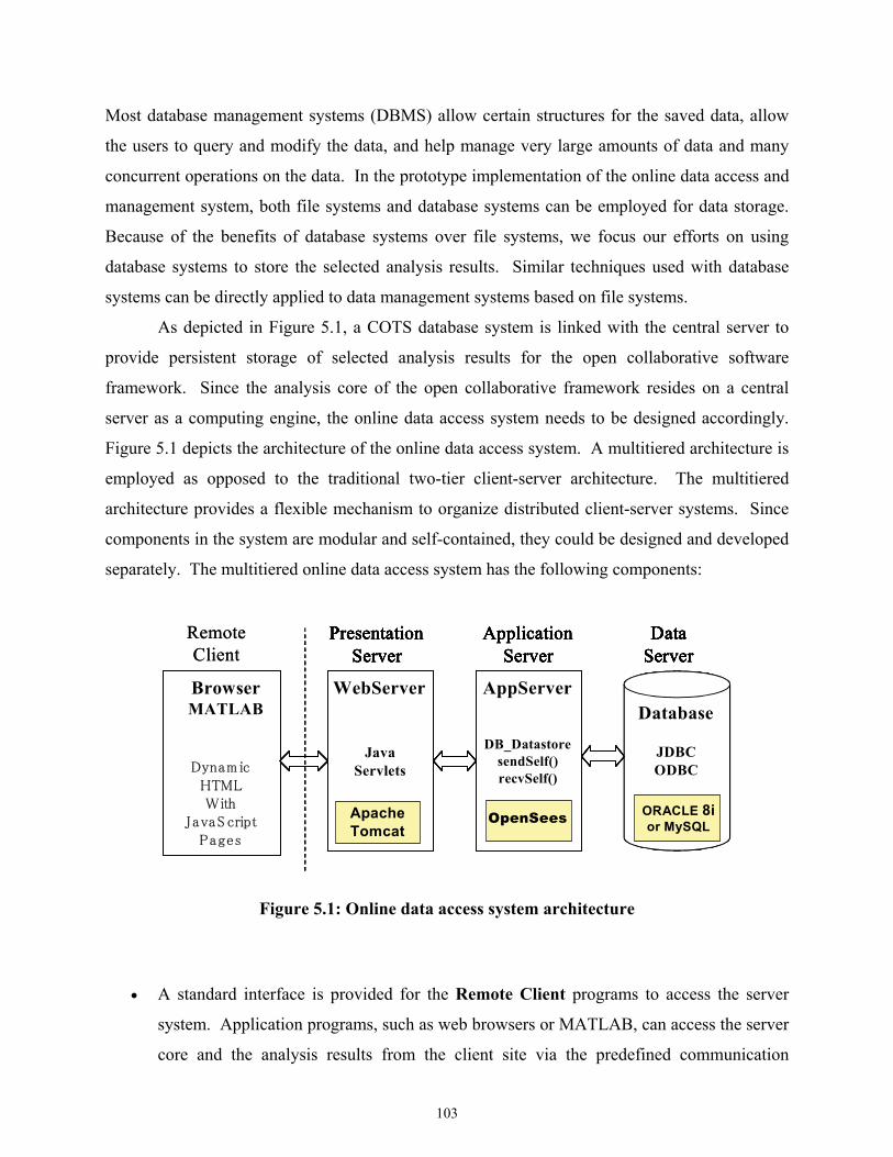
103
Most database management systems (DBMS) allow certain structures for the saved data, allow
the users to query and modify the data, and help manage very large amounts of data and many
concurrent operations on the data. In the prototype implementation of the online data access and
management system, both file systems and database systems can be employed for data storage.
Because of the benefits of database systems over file systems, we focus our efforts on using
database systems to store the selected analysis results. Similar techniques used with database
systems can be directly applied to data management systems based on file systems.
As depicted in Figure 5.1, a COTS database system is linked with the central server to
provide persistent storage of selected analysis results for the open collaborative software
framework. Since the analysis core of the open collaborative framework resides on a central
server as a computing engine, the online data access system needs to be designed accordingly.
Figure 5.1 depicts the architecture of the online data access system. A multitiered architecture is
employed as opposed to the traditional two-tier client-server architecture. The multitiered
architecture provides a flexible mechanism to organize distributed client-server systems. Since
components in the system are modular and self-contained, they could be designed and developed
separately. The multitiered online data access system has the following components:
Browser WebServerDatabase
AppServer
JavaServlet
OpenSees
Dynam icHTMLWith
JavaS criptPages
ORACLE8i
ApacheWith
TomcatStored
Procedure
ODBCJDBC
PresentationServer
ApplicationServer
DataServer
Browser WebServerDatabase
AppServer
JavaServlet
OpenSees
Dynam icHTMLWith
JavaS criptPages
ORACLEApacheWith
TomcatStored
Procedure
RemoteClient
PresentationServer
ApplicationServer
DataServer
BrowserMATLAB
JavaServlets
WebServer
JDBCODBC
DatabaseDB_Datastore
sendSelf()recvSelf()
AppServer
ApacheTomcat
OpenSees
Dynam icHTMLWith
JavaS criptPages
ORACLE 8ior MySQL
PresentationServer
ApplicationServer
DataServer
Browser WebServerDatabase
AppServer
JavaServlet
OpenSees
Dynam icHTMLWith
JavaS criptPages
ORACLE8i
ApacheWith
TomcatStored
Procedure
ODBCJDBC
PresentationServer
ApplicationServer
DataServer
Browser WebServerDatabase
AppServer
JavaServlet
OpenSees
Dynam icHTMLWith
JavaS criptPages
ORACLEApacheWith
TomcatStored
Procedure
RemoteClient
PresentationServer
ApplicationServer
DataServer
BrowserMATLAB
JavaServlets
WebServer
JDBCODBC
DatabaseDB_Datastore
sendSelf()recvSelf()
AppServer
ApacheTomcat
OpenSees
Dynam icHTMLWith
JavaS criptPages
ORACLE 8ior MySQL
PresentationServer
ApplicationServer
DataServer
Figure 5.1: Online data access system architecture
• A standard interface is provided for the Remote Client programs to access the server
system. Application programs, such as web browsers or MATLAB, can access the server
core and the analysis results from the client site via the predefined communication
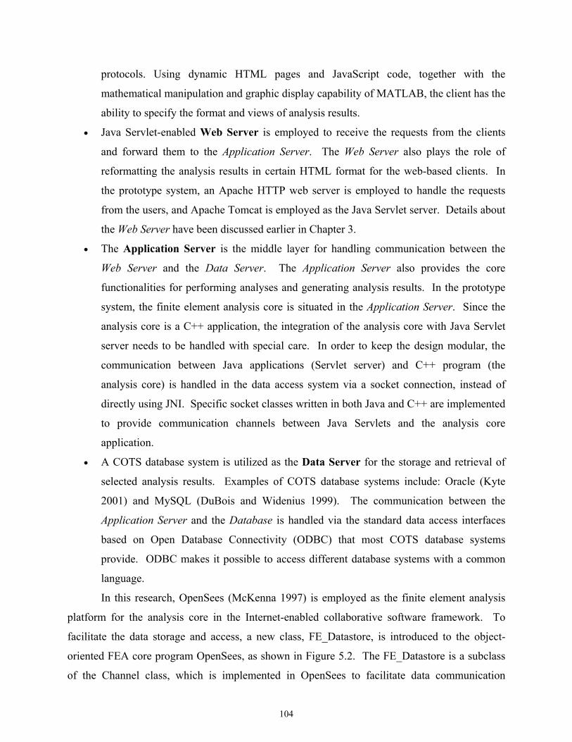
104
protocols. Using dynamic HTML pages and JavaScript code, together with the
mathematical manipulation and graphic display capability of MATLAB, the client has the
ability to specify the format and views of analysis results.
• Java Servlet-enabled Web Server is employed to receive the requests from the clients
and forward them to the Application Server. The Web Server also plays the role of
reformatting the analysis results in certain HTML format for the web-based clients. In
the prototype system, an Apache HTTP web server is employed to handle the requests
from the users, and Apache Tomcat is employed as the Java Servlet server. Details about
the Web Server have been discussed earlier in Chapter 3.
• The Application Server is the middle layer for handling communication between the
Web Server and the Data Server. The Application Server also provides the core
functionalities for performing analyses and generating analysis results. In the prototype
system, the finite element analysis core is situated in the Application Server. Since the
analysis core is a C++ application, the integration of the analysis core with Java Servlet
server needs to be handled with special care. In order to keep the design modular, the
communication between Java applications (Servlet server) and C++ program (the
analysis core) is handled in the data access system via a socket connection, instead of
directly using JNI. Specific socket classes written in both Java and C++ are implemented
to provide communication channels between Java Servlets and the analysis core
application.
• A COTS database system is utilized as the Data Server for the storage and retrieval of
selected analysis results. Examples of COTS database systems include: Oracle (Kyte
2001) and MySQL (DuBois and Widenius 1999). The communication between the
Application Server and the Database is handled via the standard data access interfaces
based on Open Database Connectivity (ODBC) that most COTS database systems
provide. ODBC makes it possible to access different database systems with a common
language.
In this research, OpenSees (McKenna 1997) is employed as the finite element analysis
platform for the analysis core in the Internet-enabled collaborative software framework. To
facilitate the data storage and access, a new class, FE_Datastore, is introduced to the object-
oriented FEA core program OpenSees, as shown in Figure 5.2. The FE_Datastore is a subclass
of the Channel class, which is implemented in OpenSees to facilitate data communication
105
between two processes. A FE_Datastore object is associated with a Domain object to store and
retrieve the state of this Domain object. The FE_Datastore class has many subclasses, including
File_Datastore and DB_Datastore. The File_Datastore class is introduced to facilitate the
storage of analysis results in a file system. The DB_Datastore is the subclass that defines the
interface between OpenSees and a database system. The DB_Datastore class uses Open
Database Connectivity (ODBC) to send and retrieve data between the OpenSees core objects and
a COTS database. Since the state of domain objects (Node, Element, Constraint, and Load, etc.)
can be represented as either a byte stream or a sequence of ID, Vector, and Matrix objects, the
DB_Datastore class provides methods to send and receive byte streams, ID, Vector and Matrix
objects. The interface for the DB_Datastore class is shown in Figure 5.3. Subclasses of the
DB_Datastore class are implemented for different database systems; for example,
OracleDatastore class is implemented for the Oracle database system and MysqlDatastore class
is implemented for the MySQL database system. Other database systems can be included by
defining new subclasses of DB_Datastore class.
ModelBuilder AnalysisDomain
FE_Datastore
File_DatastoreDB_Datastore
MysqlDatastoreOracleDatastore
Figure 5.2: Class diagram for FE_datastore
5.2 DATA STORAGE SCHEME
The usage of a database system in the online data access system has two distinct phases. The
first phase is during the finite element analysis of a model, in which certain selected analysis
results are stored in the database. The second phase occurs during the postprocessing of a finite
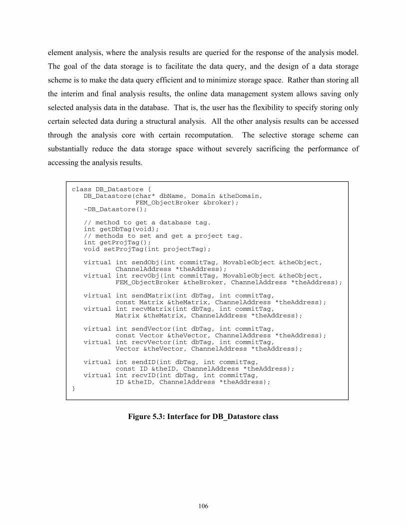
106
element analysis, where the analysis results are queried for the response of the analysis model.
The goal of the data storage is to facilitate the data query, and the design of a data storage
scheme is to make the data query efficient and to minimize storage space. Rather than storing all
the interim and final analysis results, the online data management system allows saving only
selected analysis data in the database. That is, the user has the flexibility to specify storing only
certain selected data during a structural analysis. All the other analysis results can be accessed
through the analysis core with certain recomputation. The selective storage scheme can
substantially reduce the data storage space without severely sacrificing the performance of
accessing the analysis results.
class DB_Datastore { DB_Datastore(char* dbName, Domain &theDomain, FEM_ObjectBroker &broker); ~DB_Datastore(); // method to get a database tag. int getDbTag(void); // methods to set and get a project tag. int getProjTag(); void setProjTag(int projectTag); virtual int sendObj(int commitTag, MovableObject &theObject, ChannelAddress *theAddress); virtual int recvObj(int commitTag, MovableObject &theObject, FEM_ObjectBroker &theBroker, ChannelAddress *theAddress); virtual int sendMatrix(int dbTag, int commitTag, const Matrix &theMatrix, ChannelAddress *theAddress); virtual int recvMatrix(int dbTag, int commitTag, Matrix &theMatrix, ChannelAddress *theAddress); virtual int sendVector(int dbTag, int commitTag, const Vector &theVector, ChannelAddress *theAddress); virtual int recvVector(int dbTag, int commitTag, Vector &theVector, ChannelAddress *theAddress); virtual int sendID(int dbTag, int commitTag, const ID &theID, ChannelAddress *theAddress); virtual int recvID(int dbTag, int commitTag, ID &theID, ChannelAddress *theAddress); }
Figure 5.3: Interface for DB_Datastore class
107
5.2.1 Selective Data Storage
A typical finite element analysis generates a large volume of data. The analysis results can be
saved and retrieved in two ways. One approach is to predefine all the required data and save
only those predefined data during the analysis. However, when analysis results other than the
predefined ones are needed, a complete re-analysis is needed to generate those analysis results.
For a nonlinear dynamic analysis of large structural models, the analysis needs to be restarted
from scratch, which is an expensive process in terms of both processing time and storage
requirements. The other approach is simply dumping all the interim and final analysis data into
files, which are then utilized later to retrieve the required results as a postprocessing task. The
drawbacks of this approach are the substantial amount of storage space and the potential poor
performance due to the expensive search on the large data files.
An alternative is to store only selected data, rather than storing all interim and final
analysis results. Many approaches can be adopted for selecting the data to be stored during an
analysis. The objective is to minimize the amount of storage space without severely sacrificing
performance. For many commercial finite element analysis packages, such as ANSYS and
ABAQUS, two types of output files can be created during an analysis. One type is a results file
containing results for postprocessing. The results file is the primary medium for storing results
in computer readable form. The results file can also be used as a convenient medium for
importing analysis results into other postprocessing programs. Users are able to specify in the
analysis input the kind of data to be saved in the results file. The other type of output file is a
restart file containing results for continuing an analysis or for postprocessing. The restart file
essentially stores the state of an analysis domain so that it can be used for subsequent
continuation of an analysis. Users are allowed to specify the frequency at which results will be
written to the restart file.
In the engineering data access system, these two types of data storage (results and restart)
are also supported. The data access system allows the collection of certain information to be
saved as the analysis progresses, e.g., the maximum nodal displacement at a node or the time
history response of a nodal displacement. A Recorder class is introduced in OpenSees to
facilitate the selective data storage during an analysis. The Recorder class can keep track of the
progress of an analysis and output the users’ prespecified results. Details about the usage of the
108
Recorder command have been described elsewhere by McKenna (McKenna and Fenves 2001).
Besides the recording functionalities, the data access system also has the restart capability.
Certain selected data are stored during the analysis that allows the analysis domain to be restored
to a particular state. The selected data need to be sufficient for the recomputation during
postprocessing. In the data access system, we use object serialization (Breg and
Polychronopoulos 2001) to facilitate the restart function. Object serialization captures the state
of an object and writes the state information in a persistent representation, for example in the
form of a byte stream. Consider a Truss element as an example: its nodes, dimension, number of
DOFs, length, area, and material properties can be saved in a file or a database system during an
analysis. Based on these stored data, a copy of the Truss object can be restored, and the stiffness
matrix of the Truss element can then be regenerated. The object serialization technique can be
associated with other storage management strategies to further reduce the amount of storage
space. As an example, a data storage strategy named sampling at a specified interval (SASI) can
be applied to nonlinear incremental analyses to dramatically reduce the storage requirement.
The restart function introduced in the engineering data access system is different,
however, from those supported by current commercial finite element programs (e.g., ANSYS,
ABAQUS, etc.). The restart function in the data access system relies on object serialization,
which allows the developer of each class to decide what kind of information needs to be saved.
As long as a replica of an object can be recreated with the saved data, the developer of the class
can freely manipulate the saved data. This decentralized development control provides great
flexibility and extendibility to the developers, especially in a distributed and collaborative
development environment. For most commercial finite element programs, the data saved in the
restart file must conform to certain data format. Furthermore, the restart file of most commercial
finite element programs is organized as a sequential file, which may make the data retrieval
efficient. On the other hand, the restart data saved in the data access system is retrieved
randomly — the state of a particular object is accessed through a key value. Therefore, a
particular object or a subdomain of the finite element domain can be easily restored without
retrieving unnecessary data. Because COTS database systems generally have indexing capability
to support key-based searching, the required data retrieval mechanism of the data access system
is one reason that makes COTS database systems preferable to file systems.
In the data access system, a COTS database system is associated with the finite element
analysis core to provide data storage and query. For a typical structural analysis, the analysis
109
core stores selected data into the database. During the postprocessing phase, a request from a
client for a certain analysis result is submitted to the analysis core instead of directly querying
the database. Upon receiving the request, the analysis core automatically queries the database
for saved data to instantiate the required new objects. If necessary, these objects are initialized to
restart the analysis to generate the requested results. Compared with reperforming the entire
analysis to obtain the data that are not predefined, recomputation is more efficient, since only a
small portion of the program is executed with the goal of fulfilling the request. As opposed to
storing all the data needed to answer all queries, the selective storage strategy can significantly
reduce the amount of data to be stored in the data management system.
5.2.2 Object Serialization
Ordinarily, an object lasts no longer than the program that creates it. In this context, persistence
is the ability of an object to record its state so that the object can be reproduced in the future,
even in another runtime environment. To provide persistence for objects, we can adopt a
technique called “object serialization,” where the internal data structures of an object are mapped
to a serialized representation that can be sent, stored, and retrieved by other applications.
Through object serialization, the object can be shared outside the address space of an application
by other application programs. A persistent object might store its state in a file or a database,
which is then used to restore the object in a different runtime environment. The object
serialization technique is one of the built-in features of Java and is used extensively in Java to
support object storage and object transmission. There are currently three common forms of
object serialization implementation in C++ (Slominski et al. 2001):
• Java Model: The Java serialization model stores all non-transient member data and
functions for a serializable object by default. The user can change the default behavior
by overriding the object’s readObject() and writeObject() methods, which
specify the behaviors for serialization and deserialization of the object, respectively. This
behavior can be emulated in C++ by ensuring that each serializable object implements
two methods: one for serialization and another for deserialization.
• HPC++ Model: HPC++ (Diwan 1999) is a C++ library and a set of tools being
developed by the HPC++ Consortium to support a standard model for portable parallel
110
C++ programming. The serialization model was originally introduced in HPC++ to share
objects in a network environment to facilitate parallel and distributed computing. Every
serializable object declares a global function to be its friend. The runtime environment
then uses this global function to access an object’s internal state to serialize or deserialize
it. In C++, a class can declare an individual function as a friend, and this friend function
has access to the class’ private members without itself being a member of that class.
• Template Factory Model: The template factory-based serialization model is used in
Java Beans (Lunney and McCaughey 2000), and this model can be emulated in C++. A
template is defined for each object type by a template factory. For serialization, the
runtime environment can invoke the serialization method setX() of each object to write
the state of the object to a stream. For deserialization, the type of an object needs to be
obtained from its byte stream representation first. A template of the object then can be
created by the template factory based on the object type. Subsequently, the internal states
of the object need to be accessed from the stream with getX() method. Since a
template of the object can be created based on its type and the template usually already
includes some member data and methods, the setX() method only needs to write the
member data that are not defined in the template. This is the major difference between
the template factory model and the Java model, whose writeObject() method
accesses all the member data and methods.
In the data access system, object serialization is supported via a technique that is similar
to the Template Factory Model. In the implementation of the analysis core program OpenSees,
all the modeling classes (Domain, Node, Element, Constraint, and Load, etc.), and Numerical
classes (Matrix, Vector, ID, and Tensor, etc.) share a common superclass named MovableObject.
The Interface for the MovableObject class is shown in Figure 5.4. The MovableObject class
defines two important member methods: sendSelf() and recvSelf(). The sendSelf()
method is responsible for writing the state of the object so that the corresponding recvSelf()
method can restore it. The methods sendSelf() and recvSelf() rely on a particular type
of Channel object to communicate with remote processes, which could be a remote application, a
file system or a database system.
In the data access system, the Domain state can be saved (serialization) in a database
system during a structural analysis. The stored Domain state can then be restored
(deserialization) during the postprocessing of the structural analysis to facilitate data query
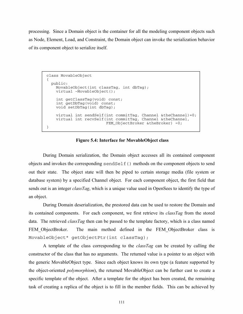
111
processing. Since a Domain object is the container for all the modeling component objects such
as Node, Element, Load, and Constraint, the Domain object can invoke the serialization behavior
of its component object to serialize itself.
class MovableObject { public: MovableObject(int classTag, int dbTag); virtual ~MovableObject(); int getClassTag(void) const; int getDbTag(void) const; void setDbTag(int dbTag); virtual int sendSelf(int commitTag, Channel &theChannel)=0; virtual int recvSelf(int commitTag, Channel &theChannel, FEM_ObjectBroker &theBroker) =0; }
Figure 5.4: Interface for MovableObject class
During Domain serialization, the Domain object accesses all its contained component
objects and invokes the corresponding sendSelf() methods on the component objects to send
out their state. The object state will then be piped to certain storage media (file system or
database system) by a specified Channel object. For each component object, the first field that
sends out is an integer classTag, which is a unique value used in OpenSees to identify the type of
an object.
During Domain deserialization, the prestored data can be used to restore the Domain and
its contained components. For each component, we first retrieve its classTag from the stored
data. The retrieved classTag then can be passed to the template factory, which is a class named
FEM_ObjectBroker. The main method defined in the FEM_ObjectBroker class is
MovableObject* getObjectPtr(int classTag);
A template of the class corresponding to the classTag can be created by calling the
constructor of the class that has no arguments. The returned value is a pointer to an object with
the generic MovableObject type. Since each object knows its own type (a feature supported by
the object-oriented polymorphism), the returned MovableObject can be further cast to create a
specific template of the object. After a template for the object has been created, the remaining
task of creating a replica of the object is to fill in the member fields. This can be achieved by
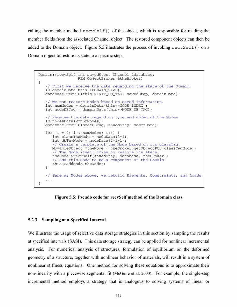
112
calling the member method recvSelf() of the object, which is responsible for reading the
member fields from the associated Channel object. The restored component objects can then be
added to the Domain object. Figure 5.5 illustrates the process of invoking recvSelf() on a
Domain object to restore its state to a specific step.
Domain::recvSelf(int savedStep, Channel &database, FEM_ObjectBroker &theBroker) { // First we receive the data regarding the state of the Domain. ID domainData(this->DOMAIN_SIZE); database.recvID(this->INIT_DB_TAG, savedStep, domainData); // We can restore Nodes based on saved information. int numNodes = domainData(this->NODE_INDEX); int nodeDBTag = domainData(this->NODE_DB_TAG); // Receive the data regarding type and dbTag of the Nodes. ID nodesData(2*numNodes); database.recvID(nodeDBTag, savedStep, nodesData); for (i = 0; i < numNodes; i++) { int classTagNode = nodeData(2*i); int dbTagNode = nodeData(2*i+1); // Create a template of the Node based on its classTag. MovableObject *theNode = theBroker.getObjectPtr(classTagNode); // The Node itself tries to restore its state. theNode->recvSelf(savedStep, database, theBroker); // Add this Node to be a component of the Domain. this->addNode(theNode); } // Same as Nodes above, we rebuild Elements, Constraints, and Loads ... }
Figure 5.5: Pseudo code for recvSelf method of the Domain class
5.2.3 Sampling at a Specified Interval
We illustrate the usage of selective data storage strategies in this section by sampling the results
at specified intervals (SASI). This data storage strategy can be applied for nonlinear incremental
analysis. For numerical analysis of structures, formulation of equilibrium on the deformed
geometry of a structure, together with nonlinear behavior of materials, will result in a system of
nonlinear stiffness equations. One method for solving these equations is to approximate their
non-linearity with a piecewise segmental fit (McGuire et al. 2000). For example, the single-step
incremental method employs a strategy that is analogous to solving systems of linear or
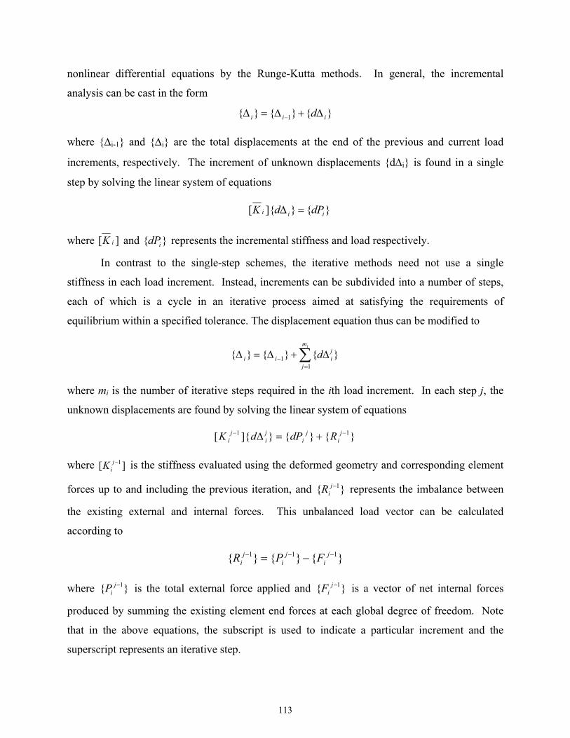
113
nonlinear differential equations by the Runge-Kutta methods. In general, the incremental
analysis can be cast in the form
}{}{}{ 1 iii d∆+∆=∆ −
where {∆i-1} and {∆i} are the total displacements at the end of the previous and current load
increments, respectively. The increment of unknown displacements {d∆i} is found in a single
step by solving the linear system of equations
}{}]{[ iii dPdK =∆
where ][ iK and }{ idP represents the incremental stiffness and load respectively.
In contrast to the single-step schemes, the iterative methods need not use a single
stiffness in each load increment. Instead, increments can be subdivided into a number of steps,
each of which is a cycle in an iterative process aimed at satisfying the requirements of
equilibrium within a specified tolerance. The displacement equation thus can be modified to
∑=
− ∆+∆=∆im
j
jiii d
11 }{}{}{
where mi is the number of iterative steps required in the ith load increment. In each step j, the
unknown displacements are found by solving the linear system of equations
}{}{}]{[ 11 −− +=∆ ji
ji
ji
ji RdPdK
where ][ 1−jiK is the stiffness evaluated using the deformed geometry and corresponding element
forces up to and including the previous iteration, and }{ 1−jiR represents the imbalance between
the existing external and internal forces. This unbalanced load vector can be calculated
according to
}{}{}{ 111 −−− −= ji
ji
ji FPR
where }{ 1−jiP is the total external force applied and }{ 1−j
iF is a vector of net internal forces
produced by summing the existing element end forces at each global degree of freedom. Note
that in the above equations, the subscript is used to indicate a particular increment and the
superscript represents an iterative step.
114
From the above equations, it can be seen that the state of the domain at a certain step is
dependent only on the state of the domain at the immediate previous step. This is applicable for
both incremental single-step methods and some of the incremental-iterative methods (such as
Newton-Raphson scheme). Based on this observation, a discrete storage strategy can be applied
to nonlinear structural analysis. More specifically, instead of storing all the analysis results, the
state information of a nonlinear analysis is saved at a specified interval (e.g., every 10 steps or
other appropriate number of steps, instead of every step). The saved state information needs to
be sufficient to restore the domain to that particular step. As discussed earlier, object
serialization can be used to guarantee this requirement.
During the postprocessing phase, the data requests are forwarded from the remote client
site to the analysis core. After receiving the requests, the analysis core will search the database
to find the closest sampled point that is less than or equal to the queried step. The core then
fetches the data from the database to obtain the necessary state information for that step. These
fetched data will be sufficient to restore the domain to that sampled step. After the domain
restores itself to the required step, the core can progress itself to reach the queried time or
incremental step. The details of this process are illustrated in the pseudo code shown in Figure
5.6. Once the state of the queried step is restored, the data queries regarding the domain at that
step can be processed by calling the corresponding member functions of the restored domain
objects. Since the domain state is saved only at the sampled steps, the total storage space is
dramatically reduced as opposed to saving the domain state at all the steps. Compared with
restarting the analysis from the original step, the processing time needed by using SASI (i.e.,
restarting the analysis from a sampled step) can potentially be reduced significantly. The same
strategy can also be designed for other types of analyses (such as for time-dependent problems).
5.3 DATA REPRESENTATION
In the data access system of the collaborative framework, data are organized internally within the
FEA analysis core using an object-oriented model. Data saved in the COTS databases are
represented in three basic data types: Matrix, Vector, and ID. Project management and version
control capabilities are also supported by the system. For external data representation, XML
(eXtensible Markup Language) (Hunter et al. 2001) is chosen as the standard for representing
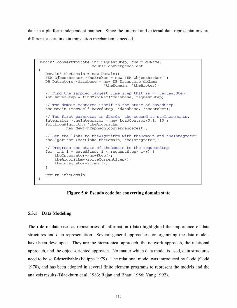
115
data in a platform-independent manner. Since the internal and external data representations are
different, a certain data translation mechanism is needed.
Domain* convertToState(int requestStep, char* dbName, double convergenceTest) { Domain* theDomain = new Domain(); FEM_OjbectBroker *theBroker = new FEM_ObjectBroker(); DB_Datastore *database = new DB_Datastore(dbName, *theDomain, *theBroker); // Find the sampled largest time step that is <= requestStep. int savedStep = findMiniMax(*database, requestStep); // The domain restores itself to the state of savedStep. theDomain->recvSelf(savedStep, *database, *theBroker); // The first parameter is dLamda, the second is numIncrements. Integrator *theIntegrator = new LoadControl(0.1, 10); SolutionAlgorithm *theAlgorithm =
new NewtonRaphson(convergenceTest); // Set the links to theAlgorithm with theDomain and theIntegrator. theAlgorithm->setLinks(theDomain, theIntegrator); // Progress the state of theDomain to the requestStep. for (int i = savedStep, i < requestStep; i++) { theIntegrator->newStep(); theAlgorithm->solveCurrentStep(); theIntegrator->commit(); } return *theDomain; }
Figure 5.6: Pseudo code for converting domain state
5.3.1 Data Modeling
The role of databases as repositories of information (data) highlighted the importance of data
structures and data representation. Several general approaches for organizing the data models
have been developed. They are the hierarchical approach, the network approach, the relational
approach, and the object-oriented approach. No matter which data model is used, data structures
need to be self-describable (Felippa 1979). The relational model was introduced by Codd (Codd
1970), and has been adopted in several finite element programs to represent the models and the
analysis results (Blackburn et al. 1983; Rajan and Bhatti 1986; Yang 1992).
116
In the collaborative framework, a relational COTS database system is used as the
backend data management system. A relational database can be perceived by the users to be a
collection of tables, with operators allowing a user to generate new tables and retrieve the data
from the tables. The term schema often refers to a description of the tables and fields along with
their relationships in a relational database system. An entity is any distinguishable object to be
represented in the database. While at the conceptual level a user may perceive the database as a
collection of tables, this does not mean that the data in the database is stored internally in tabular
form. At the internal level, the data management system (DBMS) can choose the most suitable
data structures necessary to store the data. This allows the DBMS to look after issues such as
disk seek time, disk rotational latency, transfer time, page size, and data placement to obtain a
system which can respond to user requests much more efficiently than if the users were to
implement the database directly using the file system.
The typical approach in using relational databases for FEA is to create a table for each
type of object that needs to be stored (for example, see Reference (Yang 1992)). This approach,
while straightforward, would require that at least a table be created for each type of object in the
domain. Furthermore, in nonlinear analysis, two tables would have to be created, one for the
geometry and the other for the state information of a time step. Since data structures would grow
with the incorporation of new element and material types for finite element analysis programs,
the static schema definition of most DBMS is incompatible with the evolutionary nature of FEA
software. The static schema definition of most COTS database systems makes them have
difficulties in coping with changes and modification in the evolution of a FEA program —
inconsistencies could be introduced into the database and they are expensive to eliminate.
Since OpenSees is designed and implemented using C++, the internal data structure is
organized in an object-oriented fashion. The object-oriented data structure cannot be easily
mapped into a relational database. As discussed in the last section, object serialization can be
employed efficiently as a linear stream to represent the internal state of an object. The linear
stream can simply be a byte stream or it can be a sequence of matrix-type data, namely ID (array
of integers), Vector (array of real numbers), and Matrix. The byte stream can be stored in the
database as a CLOB in order to achieve good performance for data storage and searching. A
CLOB is a built-in type that stores a Character Large Object Block as an entity in a database
table. Two methods sendObj() and recvObj() are provided in the interface of
DB_Datastore for the storage and retrieval of byte streams. The matrix-type data (ID, Vector,
117
and Matrix), on the other hand, can be directly stored in a relational database. The
corresponding methods for accessing the matrix-type data are also provided in DB_Datastore
interface. In the current implementation of the online data access system, we focus on using the
matrix-type data to represent and store the state of an object.
By using matrix-type data for storing object states, the database schema can be defined
statically. The advantage of this approach is that new classes can be introduced to the analysis
core without the creation of new tables in the relational database. The layer of abstraction
provided by DB_Datastore can alleviate the burden of the FEA software developers, who in this
case are typically finite element analysts, for learning database technologies. As long as a new
class (new element, new material types, etc.) follows the protocols of implementing
sendSelf() and recvSelf(), the objects of the new introduced class can communicate
with the database through a DB_Datastore object. The disadvantage of this approach is that no
information regarding the meaning of the data will exist within the database. Therefore, users
cannot query the database directly to obtain analysis results, e.g., the maximum stress in a
particular type of elements. However, as discussed earlier, the data can be retrieved from the
database by the objects in the core that placed the data there; that is, the semantic information is
embedded in the objects themselves.
5.3.2 Project-Based Data Storage
As shown in Figure 5.1, a database is provided as the backend data storage to facilitate online
data access. Since potentially many users can access the core server to perform structural
analysis and to query the analysis results, a project management scheme is needed. The basic
premise is that most researchers and engineers typically work independently while sharing
information necessary for collaboration. More importantly, they wish to retain control over the
information they make accessible to other members (Krishnamurthy 1996). In the prototype online
data access system, a mechanism to perform version control and access control in order to cope
with project evolution is implemented. The overall database schema is depicted in Figure 5.7.
The schema includes a USER table and a PROJECT table. A user is identified by name and a
project is identified by both its name and version. We use a hierarchical tree structure to
maintain the version set of the projects. To simplify the design, each project has a primary user
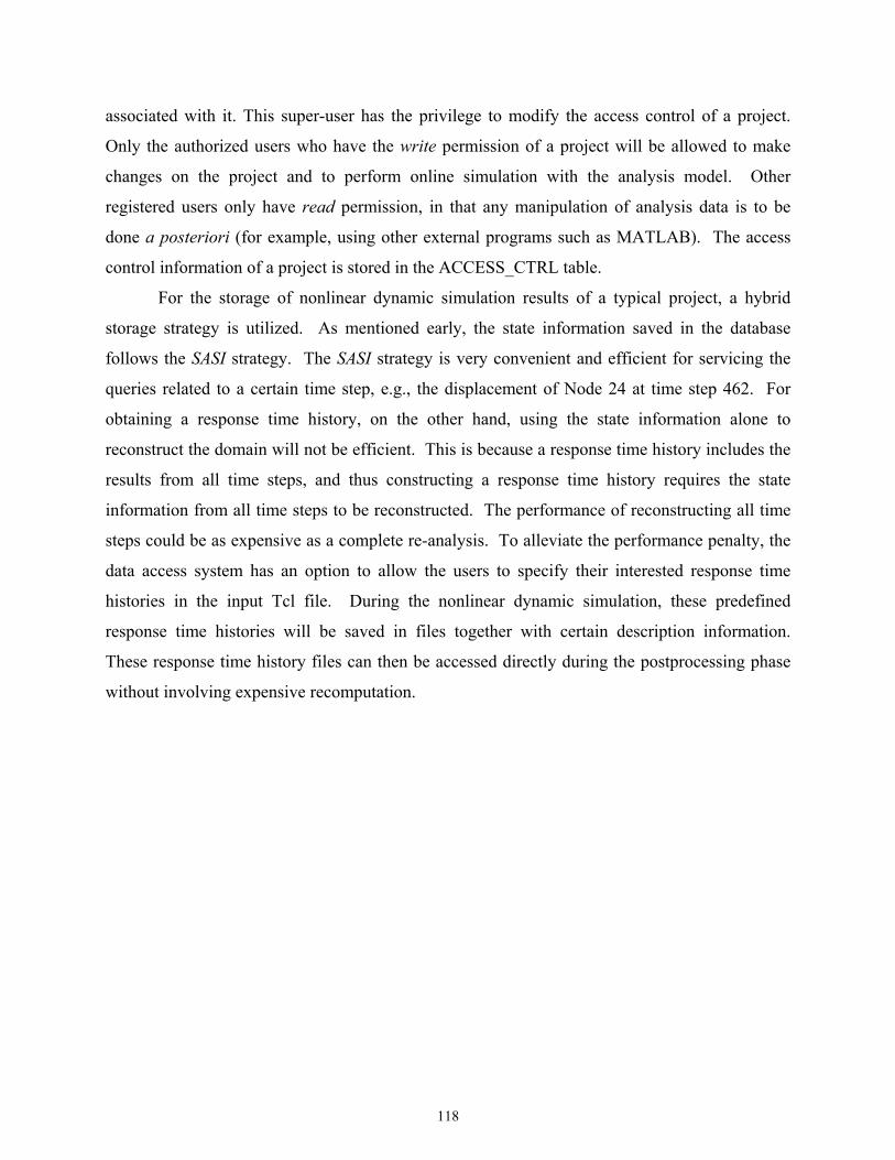
118
associated with it. This super-user has the privilege to modify the access control of a project.
Only the authorized users who have the write permission of a project will be allowed to make
changes on the project and to perform online simulation with the analysis model. Other
registered users only have read permission, in that any manipulation of analysis data is to be
done a posteriori (for example, using other external programs such as MATLAB). The access
control information of a project is stored in the ACCESS_CTRL table.
For the storage of nonlinear dynamic simulation results of a typical project, a hybrid
storage strategy is utilized. As mentioned early, the state information saved in the database
follows the SASI strategy. The SASI strategy is very convenient and efficient for servicing the
queries related to a certain time step, e.g., the displacement of Node 24 at time step 462. For
obtaining a response time history, on the other hand, using the state information alone to
reconstruct the domain will not be efficient. This is because a response time history includes the
results from all time steps, and thus constructing a response time history requires the state
information from all time steps to be reconstructed. The performance of reconstructing all time
steps could be as expensive as a complete re-analysis. To alleviate the performance penalty, the
data access system has an option to allow the users to specify their interested response time
histories in the input Tcl file. During the nonlinear dynamic simulation, these predefined
response time histories will be saved in files together with certain description information.
These response time history files can then be accessed directly during the postprocessing phase
without involving expensive recomputation.
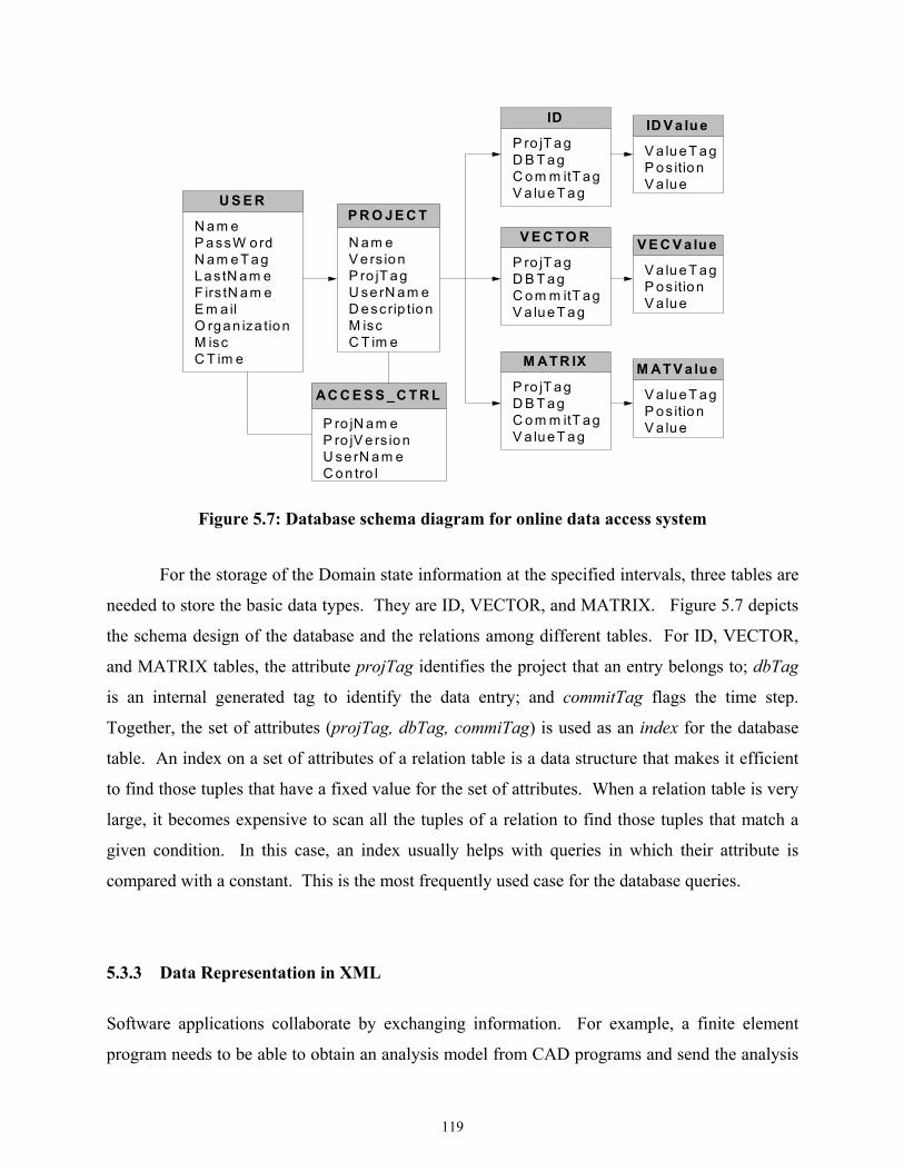
119
N am eP assW ordN am e T a gLas tN am eF irs tN am eE m a ilO rgan iza tionM iscC T im e
U S E R
N am eV e rs ionP ro jT agU se rN am eD escrip tionM iscC T im e
P R O JE C T
P ro jT agD B T agC o m m itT agV a lueT ag
M AT R IX
P ro jT agD B T agC o m m itT agV a lueT ag
V E C T O R
P ro jT agD B T agC o m m itT agV a lueT ag
ID
V a lueT agP os itionV a lue
ID V a lu e
V a lueT agP os itionV a lue
V E C V a lu e
V a lueT agP os itionV a lue
M AT V a lu e
P ro jN am eP ro jV e rs ionU se rN am eC on tro l
AC C E S S _C T R L
Figure 5.7: Database schema diagram for online data access system
For the storage of the Domain state information at the specified intervals, three tables are
needed to store the basic data types. They are ID, VECTOR, and MATRIX. Figure 5.7 depicts
the schema design of the database and the relations among different tables. For ID, VECTOR,
and MATRIX tables, the attribute projTag identifies the project that an entry belongs to; dbTag
is an internal generated tag to identify the data entry; and commitTag flags the time step.
Together, the set of attributes (projTag, dbTag, commiTag) is used as an index for the database
table. An index on a set of attributes of a relation table is a data structure that makes it efficient
to find those tuples that have a fixed value for the set of attributes. When a relation table is very
large, it becomes expensive to scan all the tuples of a relation to find those tuples that match a
given condition. In this case, an index usually helps with queries in which their attribute is
compared with a constant. This is the most frequently used case for the database queries.
5.3.3 Data Representation in XML
Software applications collaborate by exchanging information. For example, a finite element
program needs to be able to obtain an analysis model from CAD programs and send the analysis
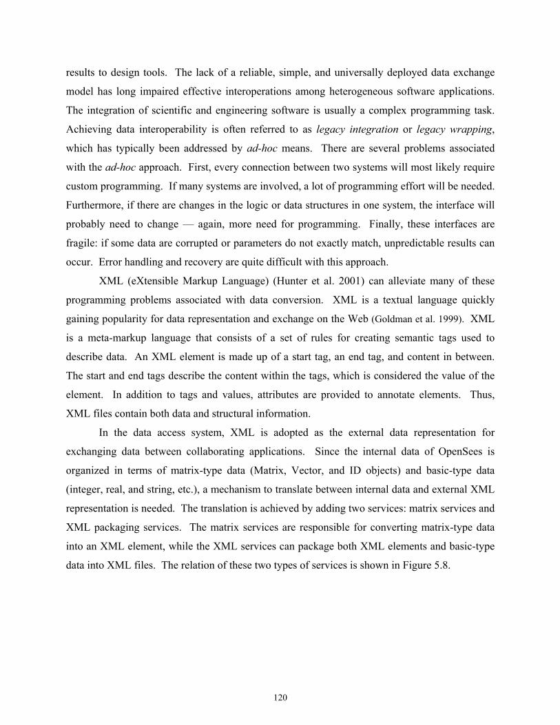
120
results to design tools. The lack of a reliable, simple, and universally deployed data exchange
model has long impaired effective interoperations among heterogeneous software applications.
The integration of scientific and engineering software is usually a complex programming task.
Achieving data interoperability is often referred to as legacy integration or legacy wrapping,
which has typically been addressed by ad-hoc means. There are several problems associated
with the ad-hoc approach. First, every connection between two systems will most likely require
custom programming. If many systems are involved, a lot of programming effort will be needed.
Furthermore, if there are changes in the logic or data structures in one system, the interface will
probably need to change — again, more need for programming. Finally, these interfaces are
fragile: if some data are corrupted or parameters do not exactly match, unpredictable results can
occur. Error handling and recovery are quite difficult with this approach.
XML (eXtensible Markup Language) (Hunter et al. 2001) can alleviate many of these
programming problems associated with data conversion. XML is a textual language quickly
gaining popularity for data representation and exchange on the Web (Goldman et al. 1999). XML
is a meta-markup language that consists of a set of rules for creating semantic tags used to
describe data. An XML element is made up of a start tag, an end tag, and content in between.
The start and end tags describe the content within the tags, which is considered the value of the
element. In addition to tags and values, attributes are provided to annotate elements. Thus,
XML files contain both data and structural information.
In the data access system, XML is adopted as the external data representation for
exchanging data between collaborating applications. Since the internal data of OpenSees is
organized in terms of matrix-type data (Matrix, Vector, and ID objects) and basic-type data
(integer, real, and string, etc.), a mechanism to translate between internal data and external XML
representation is needed. The translation is achieved by adding two services: matrix services and
XML packaging services. The matrix services are responsible for converting matrix-type data
into an XML element, while the XML services can package both XML elements and basic-type
data into XML files. The relation of these two types of services is shown in Figure 5.8.
121
MatrixVector, ID Output
Matrix ServicesGenerating XML
representation by Matrixand Vector classes
XML ServicesFormatting and buidling
XML documents byXML classes
XMLPackaging
XMLElement
IntegerReal, String
Figure 5.8: Relation of XML services
The translation between matrix-type data (Matrix, Vector, and ID) and XML elements is
achieved by adding two member functions to the Matrix, Vector, and ID classes to perform data
conversion. These two new member functions are:
char* ObjToXML();
void XMLToObj(char* inputXML);
The function XMLToObj() is used to populate a matrix-type object with an input XML
stream; and the function ObjToXML() is responsible for converting the object member data
into XML representation. In order to represent data efficiently, matrix-type entity sets can be
divided into two categories: sparse matrices and full matrices. Figure 5.9 shows the XML
representation of a full matrix (for example, the stiffness matrix of a 2D truss element) and a
sparse matrix (for example, the lumped-mass matrix of a 2D truss element). Since Vector and ID
are normally not sparse, they can be represented in a similar way as a full matrix.
(a) Full Matrix (b) Sparse Matrix
Figure 5.9: XML representation of matrix-type data
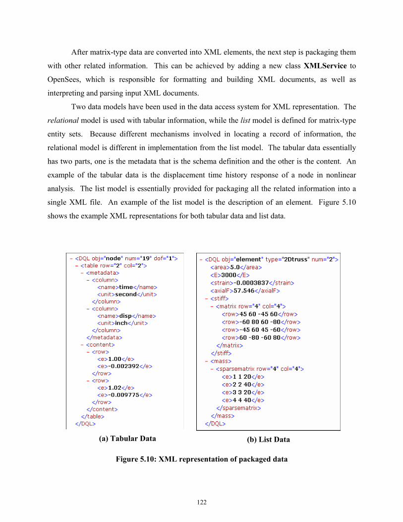
122
After matrix-type data are converted into XML elements, the next step is packaging them
with other related information. This can be achieved by adding a new class XMLService to
OpenSees, which is responsible for formatting and building XML documents, as well as
interpreting and parsing input XML documents.
Two data models have been used in the data access system for XML representation. The
relational model is used with tabular information, while the list model is defined for matrix-type
entity sets. Because different mechanisms involved in locating a record of information, the
relational model is different in implementation from the list model. The tabular data essentially
has two parts, one is the metadata that is the schema definition and the other is the content. An
example of the tabular data is the displacement time history response of a node in nonlinear
analysis. The list model is essentially provided for packaging all the related information into a
single XML file. An example of the list model is the description of an element. Figure 5.10
shows the example XML representations for both tabular data and list data.
(a) Tabular Data
(b) List Data
Figure 5.10: XML representation of packaged data
123
5.4 DATA QUERY PROCESSING
For finite element programs, the postprocessing functions need to allow the recovery of analysis
results and provide extensive graphical and numerical tools for gaining an understanding of
results. In this sense, querying the analysis results is an important aspect, and query languages
need to be constructed to retrieve the analysis results. In the online data access system, a data
query processing system is provided to support the interaction between people and application
programs. A data query language is also defined to facilitate data retrieval as well as invoking
postprocessing functionalities. With the query language, users can have uniform access to the
analysis results by using a web browser or other application programs.
5.4.1 Data Query Language
The data access system supports both programmed procedures and high-level query languages
for accessing domain models and analysis results. A query language can be used to define,
manipulate, and retrieve information from a database. For instance, for retrieving some
particular result of an analysis, a query can be formed in the high-level and declarative query
language that satisfies the specified syntax and conditions. In the data access system, a query
language is provided to query the analysis result. The DQL (data query language) is defined in a
systematic way and it is capable of querying the analysis results together with invoking certain
postprocessing computation. Combining general query language constructs with domain-related
representations provides a more problem-oriented communication. (Orsborn 1994). The defined
DQL and the programmed procedures have at least two features:
• It provides a unified data query language. No matter what kind of form the data is
presented (whether a relation or a matrix), the data is treated in the same way. It is also
possible to make query on specific entries in a table or individual elements of a matrix.
• The DQL language provides the same syntax for both terminal users (from command
lines) and for those who use the DQL within a programmed procedure. This leads to the
ease of communication between the client and the server, and can save programming
efforts when linking the data access system with other application programs.
124
As discussed earlier, a hybrid storage strategy is utilized for storing nonlinear dynamic
simulation results. For different types of stored data (results regarding a certain time step or time
history responses), different query commands are needed and different actions are taken. Several
commonly used features of the DQL are illustrated below.
Queries related to a particular time step:
First, we will illustrate the queries related to a particular time step. In order to query the data
related to a specified time step, the Domain state needs to be restored to that time step. For
example, we can use command RESTORE 462, which will trigger the function
convertToState() on the Domain object (shown in Figure 5.6) to restore the Domain state
to time step 462.
After the domain has been restored to the time step, queries can be issued for detailed
information. As an example, we can query the displacement from Node number 4,
SELECT disp FROM node=4;
The analysis result can also be queried from other domain object: Element, Constraint,
and Load. For example,
SELECT tangentStiff FROM element=2;
returns the stiffness matrix of Element number 2.
Besides the general queries, two wildcards are provided. One is the wildcard ‘*’ that
represents all values. For instance, if we want to obtain the displacement from all the nodes, we
can use
SELECT disp FROM node=*;
The other wildcard ‘?’ can be used on a certain object to find out what kind of queries it
can support. For example, the following query
SELECT ? FROM node=1;
returns Node 1:: numDOF crds disp vel accel load mass *
Another class of operations is aggregation. By aggregation, we mean an operation that
forms a single value from a list of related values. In the current implementation, five operators
are provided that apply to a list of related values and produce a summary or aggregation of that
list. These operators are:
125
SUM, the sum of the values in the list;
AVG, the average of values in the list;
MIN, the least value in the list;
MAX, the greatest value in the list;
COUNT, the number of values in the list.
Queries of time history responses:
The second type of queries is used to access the predefined analysis results, especially the time
history responses. The users are allowed to specify in the Tcl file what kind of information they
want to keep track of. During the structural analysis, these predefined data are stored in files in
the central server site. The files saved in the server can be queried and downloaded by the
clients. The queried time history responses can be saved into files in the client site. The data in
the files then can be retrieved for future postprocessing applications. For instance, if we want to
save the displacement time history response of a particular node, the following query can be
issued to the server
SELECT time disp FROM node=1 AND dof=1
SAVEAS node1.out;
If the data are predefined in the Tcl input file and saved during the analysis phase, the
query can return the corresponding saved analysis results. Otherwise, a complete recomputation
is triggered to generate the requested time history response.
5.4.2 Data Query Interfaces
The collaborative framework can offer users access to the analysis core, as well as to the
associated supporting services via the Internet. One of the supporting services is to query
analysis results. Users can compile their query in the client site and then submit it to the central
server. After the server finishes the processing, queried results will return to the users in a
predefined XML format. It is up to the client program to interpret the data and present the data
in a specific format desirable to the users. In the prototype system, two types of data query
interfaces are provided: a web-based interface and a MATLAB-based interface. This client-
server computing environment forms a complete computing framework with a very distinct
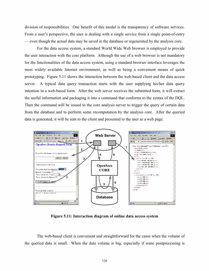
126
division of responsibilities. One benefit of this model is the transparency of software services.
From a user’s perspective, the user is dealing with a single service from a single point-of-entry
— even though the actual data may be saved in the database or regenerated by the analysis core.
For the data access system, a standard World Wide Web browser is employed to provide
the user interaction with the core platform. Although the use of a web browser is not mandatory
for the functionalities of the data access system, using a standard browser interface leverages the
most widely available Internet environment, as well as being a convenient means of quick
prototyping. Figure 5.11 shows the interaction between the web-based client and the data access
server. A typical data query transaction starts with the user supplying his/her data query
intention in a web-based form. After the web server receives the submitted form, it will extract
the useful information and packaging it into a command that conforms to the syntax of the DQL.
Then the command will be issued to the core analysis server to trigger the query of certain data
from the database and to perform some recomputation by the analysis core. After the queried
data is generated, it will be sent to the client and presented to the user as a web page.
Database
OpenSeesCORE
Web Server
4
0
1
5
6
27
3
Figure 5.11: Interaction diagram of online data access system
The web-based client is convenient and straightforward for the cases when the volume of
the queried data is small. When the data volume is big, especially if some postprocessing is
127
needed on the data, the direct usage of a web-based client can bear some inconvenience. All too
often the queried analysis results need to be downloaded from the server as a file, and then put
manually into another program to perform postprocessing, e.g., a spreadsheet. For example, if
we want to plot a time history response of a certain node after a dynamic analysis, we might have
to download the response in a data file and then use MATLAB, Excel, or other software
packages to generate the graphical representation. It would be more convenient to directly
utilize some popular application software packages to enhance the interaction between client and
server. In our prototype system, a MATLAB-based user interface is available to take advantage
of the mathematical and graphical processing power of MATLAB. In the implementation, some
extra functions are added to the standard MATLAB in order to handle the network
communication and data processing. These add-on functions can be directly invoked from either
the MATLAB prompt or a MABLAB-based graphical user interface.
5.5 APPLICATIONS
A prototype of the online data access and project management system is implemented using Sun
workstations as the hardware platform. The finite element analysis core is based on OpenSees,
and the employed database system is Oracle 8i. The Apache HTTP server is served as the web
server, and Apache Tomcat 4.0 is utilized as the Java Servlet server. MATLAB 6.0 and a
standard web-browser are employed as the user interfaces for accessing the analysis results and
project-related information.
As we discussed earlier, a Tcl input interface is employed in OpenSees to send
commands to the analysis core (McKenna and Fenves 2001). To facilitate data storage and data
access, several new commands are introduced to the Tcl interpreter of OpenSees. The
introduced new Tcl commands are:
• database <databaseName> <databaseType>
The database command is used to construct a FE_Datastore object to build the
communication between OpenSees and a storage media. The first argument to the
database command is databaseName, which can be used to specify the project that the
simulation is related to. The second argument databaseType is used to specify the
type of storage media. Some possible values for databaseType are: File, Oracle,
MySQL, or other types of database systems.
128
• save <startingStep> <endStep> <stepSize>
The save command can be used to inform the Analysis object to save the domain state
at certain time steps. The three arguments to the save commands are used to specify in
which time steps the domain state needs to be saved. The startingStep defines the
first time step the domain state is saved, the endStep defines the ending criteria, and the
stepSize is the time interval. The usage of these three arguments is analogous to the
usage of arguments in the for loop of C/C++ language.
• restore <step>
The restore command is used to restore the domain state to the specified time step
step. If the domain state of the specified step is not saved in the database, certain
recomputation will be triggered to restore the domain.
5.5.1 Example 1: Eighteen-Story One-Bay Frame Model
The first test case example is the eighteen-story, two-dimensional one-bay frame model shown in
Figure 3.8. For this example, the Newton-Raphson procedure is employed for the nonlinear
structural analysis. Furthermore, the SASI strategy is used to store the domain state at every ten
time steps. The step size (every 10 steps) is specified in the input Tcl file by using the save
command. Besides the saved domain states, the time history displacement values of each node
are saved in files by using the Tcl recorder command.
After the analysis, the results regarding any time step can be queried by using the DQL
commands. The following illustrates example usage of some of the DQL commands. We use C:
for the query command and R: for the queried results.
C: RESTORE 462
This command is used to restore the Domain state to the time step 462. The command
first triggers the analysis core to fetch from the database the saved Domain state at time step
460, which is the closest time step stored before the requested step. The analysis core program
then progresses itself to reach time step 462 using the Newton-Raphson scheme. After the
Domain has been initialized to the step of 462, the wildcard ‘?’ can be used to find the attribute
information of node 1 (which is the left node on the 18th floor) that can be retrieved:
129
C: SELECT ? FROM node=1;
R: Node 1:: numDOF crds disp vel accel load trialDisp trialVel trialAccel mass *
For example, we retrieve the displacement information of Node 1 as follows:
C: SELECT disp FROM node=1;
R: Node 1:: disp= -7.42716 0.04044
The analysis result can also be queried for Element, Constraint, and Load. For instance,
we can query the information related to element 19, which is the left column on the 18th floor.
C: SELECT ? FROM element=19;
R: ElasticBeam2D 19:: connectedNodes A E I L tangentStiff secantStiff mass damp
C: SELECT L E FROM element=19;
R: ElasticBeam2D 19:: L=144 E=29000
As mentioned earlier, five aggregation operators are provided to produce summary or
aggregation information. For instance, the following command produces the maximum
displacement among all the nodes. Please note that both positive and negative maximum values
are presented.
C: SELECT MAX(disp) FROM node=*;
R: MAX(disp):: Node 1: –7.42716 Node 21: 4.93986
We can also use a DQL command to query the time history response. For instance, if we
want to save the displacement time history response of Node 1, the following query can be
issued to the server
C: SELECT time disp FROM node=1 AND dof=1 SAVEAS node1.out;
After the execution of the command, the displacement time history response of Node 1 is
saved in a file named node1.out. At this stage, we can invoke the added MATLAB-based
interface command res2Dplot(‘node1.out’) to plot the displacement time history
response of Node 1, which is shown in Figure 5.12.
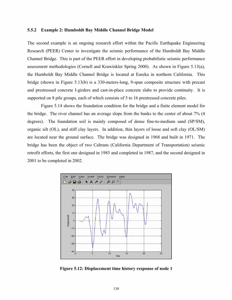
130
5.5.2 Example 2: Humboldt Bay Middle Channel Bridge Model
The second example is an ongoing research effort within the Pacific Earthquake Engineering
Research (PEER) Center to investigate the seismic performance of the Humboldt Bay Middle
Channel Bridge. This is part of the PEER effort in developing probabilistic seismic performance
assessment methodologies (Cornell and Krawinkler Spring 2000). As shown in Figure 5.13(a),
the Humboldt Bay Middle Channel Bridge is located at Eureka in northern California. This
bridge (shown in Figure 5.13(b) is a 330-meters-long, 9-span composite structure with precast
and prestressed concrete I-girders and cast-in-place concrete slabs to provide continuity. It is
supported on 8 pile groups, each of which consists of 5 to 16 prestressed concrete piles.
Figure 5.14 shows the foundation condition for the bridge and a finite element model for
the bridge. The river channel has an average slope from the banks to the center of about 7% (4
degrees). The foundation soil is mainly composed of dense fine-to-medium sand (SP/SM),
organic silt (OL), and stiff clay layers. In addition, thin layers of loose and soft clay (OL/SM)
are located near the ground surface. The bridge was designed in 1968 and built in 1971. The
bridge has been the object of two Caltrans (California Department of Transportation) seismic
retrofit efforts, the first one designed in 1985 and completed in 1987, and the second designed in
2001 to be completed in 2002.
Figure 5.12: Displacement time history response of node 1
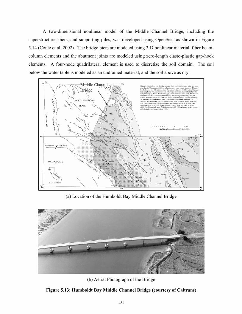
131
A two-dimensional nonlinear model of the Middle Channel Bridge, including the
superstructure, piers, and supporting piles, was developed using OpenSees as shown in Figure
5.14 (Conte et al. 2002). The bridge piers are modeled using 2-D nonlinear material, fiber beam-
column elements and the abutment joints are modeled using zero-length elasto-plastic gap-hook
elements. A four-node quadrilateral element is used to discretize the soil domain. The soil
below the water table is modeled as an undrained material, and the soil above as dry.
(a) Location of the Humboldt Bay Middle Channel Bridge
(b) Aerial Photograph of the Bridge
Figure 5.13: Humboldt Bay Middle Channel Bridge (courtesy of Caltrans)
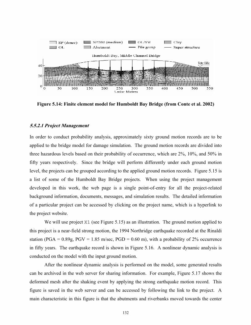
132
Figure 5.14: Finite element model for Humboldt Bay Bridge (from Conte et al. 2002)
5.5.2.1 Project Management In order to conduct probability analysis, approximately sixty ground motion records are to be
applied to the bridge model for damage simulation. The ground motion records are divided into
three hazardous levels based on their probability of occurrence, which are 2%, 10%, and 50% in
fifty years respectively. Since the bridge will perform differently under each ground motion
level, the projects can be grouped according to the applied ground motion records. Figure 5.15 is
a list of some of the Humboldt Bay Bridge projects. When using the project management
developed in this work, the web page is a single point-of-entry for all the project-related
background information, documents, messages, and simulation results. The detailed information
of a particular project can be accessed by clicking on the project name, which is a hyperlink to
the project website.
We will use project X1 (see Figure 5.15) as an illustration. The ground motion applied to
this project is a near-field strong motion, the 1994 Northridge earthquake recorded at the Rinaldi
station (PGA = 0.89g, PGV = 1.85 m/sec, PGD = 0.60 m), with a probability of 2% occurrence
in fifty years. The earthquake record is shown in Figure 5.16. A nonlinear dynamic analysis is
conducted on the model with the input ground motion.
After the nonlinear dynamic analysis is performed on the model, some generated results
can be archived in the web server for sharing information. For example, Figure 5.17 shows the
deformed mesh after the shaking event by applying the strong earthquake motion record. This
figure is saved in the web server and can be accessed by following the link to the project. A
main characteristic in this figure is that the abutments and riverbanks moved towards the center
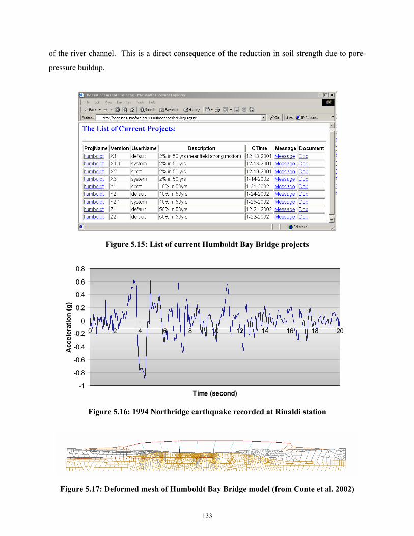
133
of the river channel. This is a direct consequence of the reduction in soil strength due to pore-
pressure buildup.
Figure 5.15: List of current Humboldt Bay Bridge projects
-1
-0.8
-0.6
-0.4
-0.2
0
0.2
0.4
0.6
0.8
0 2 4 6 8 10 12 14 16 18 20
Time (second)
Acc
eler
atio
n (g
)
Figure 5.16: 1994 Northridge earthquake recorded at Rinaldi station
Figure 5.17: Deformed mesh of Humboldt Bay Bridge model (from Conte et al. 2002)
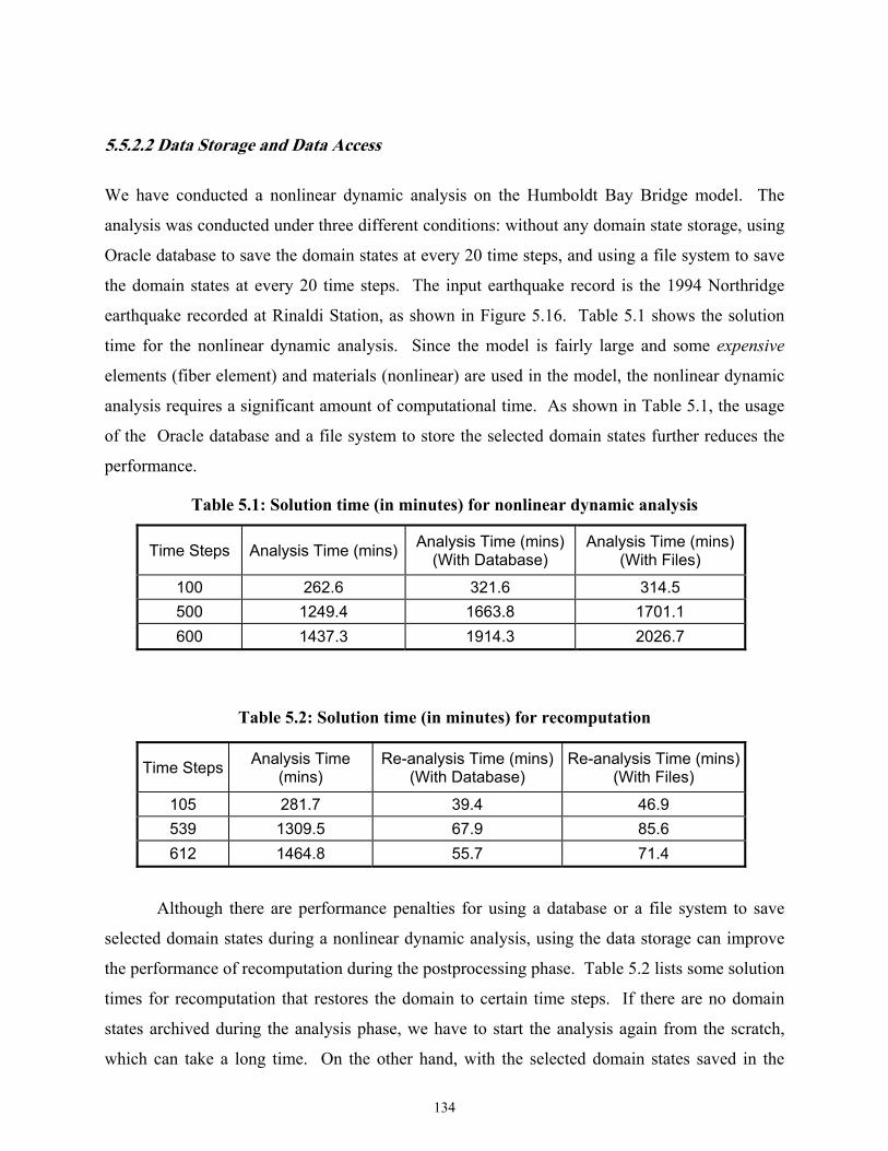
134
5.5.2.2 Data Storage and Data Access
We have conducted a nonlinear dynamic analysis on the Humboldt Bay Bridge model. The
analysis was conducted under three different conditions: without any domain state storage, using
Oracle database to save the domain states at every 20 time steps, and using a file system to save
the domain states at every 20 time steps. The input earthquake record is the 1994 Northridge
earthquake recorded at Rinaldi Station, as shown in Figure 5.16. Table 5.1 shows the solution
time for the nonlinear dynamic analysis. Since the model is fairly large and some expensive
elements (fiber element) and materials (nonlinear) are used in the model, the nonlinear dynamic
analysis requires a significant amount of computational time. As shown in Table 5.1, the usage
of the Oracle database and a file system to store the selected domain states further reduces the
performance.
Table 5.1: Solution time (in minutes) for nonlinear dynamic analysis
Time Steps Analysis Time (mins) Analysis Time (mins) (With Database)
Analysis Time (mins) (With Files)
100 262.6 321.6 314.5 500 1249.4 1663.8 1701.1 600 1437.3 1914.3 2026.7
Table 5.2: Solution time (in minutes) for recomputation
Time Steps Analysis Time (mins)
Re-analysis Time (mins)(With Database)
Re-analysis Time (mins)(With Files)
105 281.7 39.4 46.9 539 1309.5 67.9 85.6 612 1464.8 55.7 71.4
Although there are performance penalties for using a database or a file system to save
selected domain states during a nonlinear dynamic analysis, using the data storage can improve
the performance of recomputation during the postprocessing phase. Table 5.2 lists some solution
times for recomputation that restores the domain to certain time steps. If there are no domain
states archived during the analysis phase, we have to start the analysis again from the scratch,
which can take a long time. On the other hand, with the selected domain states saved in the
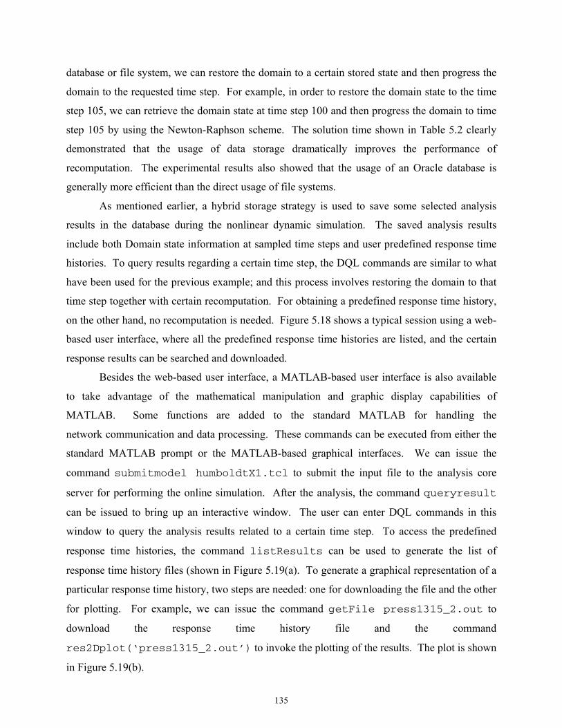
135
database or file system, we can restore the domain to a certain stored state and then progress the
domain to the requested time step. For example, in order to restore the domain state to the time
step 105, we can retrieve the domain state at time step 100 and then progress the domain to time
step 105 by using the Newton-Raphson scheme. The solution time shown in Table 5.2 clearly
demonstrated that the usage of data storage dramatically improves the performance of
recomputation. The experimental results also showed that the usage of an Oracle database is
generally more efficient than the direct usage of file systems.
As mentioned earlier, a hybrid storage strategy is used to save some selected analysis
results in the database during the nonlinear dynamic simulation. The saved analysis results
include both Domain state information at sampled time steps and user predefined response time
histories. To query results regarding a certain time step, the DQL commands are similar to what
have been used for the previous example; and this process involves restoring the domain to that
time step together with certain recomputation. For obtaining a predefined response time history,
on the other hand, no recomputation is needed. Figure 5.18 shows a typical session using a web-
based user interface, where all the predefined response time histories are listed, and the certain
response results can be searched and downloaded.
Besides the web-based user interface, a MATLAB-based user interface is also available
to take advantage of the mathematical manipulation and graphic display capabilities of
MATLAB. Some functions are added to the standard MATLAB for handling the
network communication and data processing. These commands can be executed from either the
standard MATLAB prompt or the MATLAB-based graphical interfaces. We can issue the
command submitmodel humboldtX1.tcl to submit the input file to the analysis core
server for performing the online simulation. After the analysis, the command queryresult
can be issued to bring up an interactive window. The user can enter DQL commands in this
window to query the analysis results related to a certain time step. To access the predefined
response time histories, the command listResults can be used to generate the list of
response time history files (shown in Figure 5.19(a). To generate a graphical representation of a
particular response time history, two steps are needed: one for downloading the file and the other
for plotting. For example, we can issue the command getFile press1315_2.out to
download the response time history file and the command
res2Dplot(‘press1315_2.out’) to invoke the plotting of the results. The plot is shown
in Figure 5.19(b).
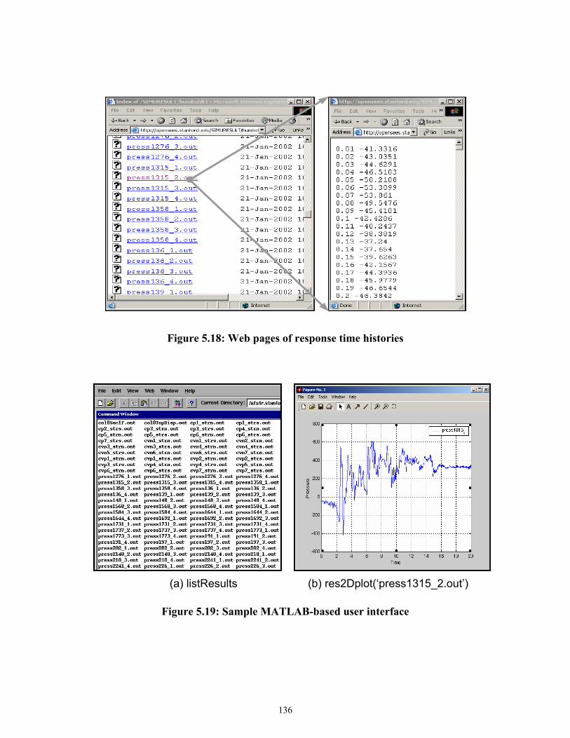
136
Figure 5.18: Web pages of response time histories
(a) listResults (b) res2Dplot(‘press1315_2.out’)
Figure 5.19: Sample MATLAB-based user interface
137
5.6 SUMMARY AND DISCUSSION
Scientific and engineering database systems have several special requirements compared with
their business counterparts. The dataflow of a finite element analysis program is tightly coupled
with expensive numerical computation. This is one of the main reasons for the lack of a generic
purpose data management system for finite element programs. When a number of programs are
required for engineering simulation or design, the absence of standardization and the lack of
coordination among software developers can result in difficulty in data communication from one
program to another. The result is often manual transfer of data with laborious efforts, time delay,
and potential error. In the effort of trying to alleviate some of the problems, we have introduced
a data access system for a finite element structural analysis program. The main design principle
of the system is to separate data access and data storage from data processing, so that each part
of the system can be designed and implemented separately. By introducing a standard data
representation and a modular infrastructure, each component of the system can be added or
updated without substantial amount of modification to the existing system. By storing abstract
data types (ID, Vector, and Matrix) into the database, it is not necessary to re-implement low-
level dedicated data structures or to redefine new database tables for each added new element or
other components. The utilization of a standard query language and popular query interfaces, as
well as the deployment of the Internet for delivering data, is another factor that makes the system
flexible and extendible. Although this work has focused on a data access system for a finite
element program, the design principles and techniques can be applied to other similar types of
engineering and scientific applications.
For the prototype implementation and testing in this research work, we have utilized an
Oracle database system as the backend data server. The experimental results clearly showed that
a COTS database system can facilitate the data management for a FEA program, and improve the
performance of certain types of queries including queries related to a particular time step of a
nonlinear dynamic analysis. Because the design is flexible and general, other types of database
systems, e.g., MySQL (DuBois and Widenius 1999), BerkeleyDB (Olson et al. 1999), or
Microsoft Access (Andersen 1999), can easily be employed to provide data storage for the data
access system.
In the prototype data access system, the performance may be a concern. This is partly
because of the unstable performance of the Internet, and partly due to the design decision of
138
sacrificing a certain degree of performance for better flexibility and extendibility. However,
compared with the direct usage of file systems, using relational database systems normally
improves the overall performance of the system. By utilizing the selective storage strategy,
especially SASI, the amount of storage space in our system is substantially smaller than the
storage requirement of simply dumping all the analysis data into files. Compared to the
traditional way of redoing the entire analysis to obtain the results that are not predefined, the
recomputation technique used in the data access system could be more efficient because only a
small portion of the program is executed with the goal to fulfill the query request. While the
performance issue does exist, it may be alleviated by efficient optimization of generated code,
and possibly, by indexing techniques. The database indexing techniques have been used in the
prototype data access system to improve the performance of data query.
6 Summary and Future Directions
This research has developed an Internet-enabled software framework and has proposed a new
system paradigm for the design and implementation of finite element analysis programs. The
framework allows distributed computers and related software components to function
collaboratively as a single system. Three goals motivated the development of the collaborative
software framework:
• Developing a software framework that would allow engineers and users to easily access a
finite element analysis program running on a server environment.
• Providing a plug-and-play environment where researchers and developers can collaborate
and build incrementally on each other’s developments.
• Providing a data management system to facilitate the access to simulation results and to
perform project management.
This chapter provides a brief summary and discusses some key features of the
collaborative software framework. Furthermore, certain limitations of the system and directions
for future work are discussed.
6.1 SUMMARY This research is focused on the design and implementation of an Internet-enabled software
framework that can facilitate the development of finite element analysis programs and the access
of simulation results. The main design principle of this collaborative framework is to keep the
software kernel flexible and extendible, so that a diverse group of users and developers can
easily access the platform and attach their own developments to the core server. The
collaborative Internet service architecture would allow new services to be remotely incorporated
into a modular nonlinear dynamic analysis platform. Users can select appropriate services and
140
can easily replace one service by another without having to recompile or reinitialize the existing
services being used. The software framework also allows users to remotely access simulation
results and other related information. There are a number of notable features of the collaborative
software framework.
Component-based modular design is adopted in the collaborative framework to enhance
the usability, flexibility, interoperability, and scalability of the engineering analysis software.
The collaborative framework for the finite element structural analysis program described consists
of six distinct component modules. Each module in the system is well-defined and encapsulated.
In addition, each component module provides and/or requires a set of services interacting with
the core via well-defined interfaces. The modules are “loosely coupled,” and the loose
connectivity among components allows each component to be implemented separately, which
can facilitate concurrent software development. For example, the engineering data access system
is linked with the core server and employs a multitiered modular design, which separates data
access and data storage from data processing. In short, the collaborative framework is a system
where complex groupings of components can interact in diverse ways, and new components can
easily be integrated into the system with a plug-and-play character. Another benefit of
component-based design is that the code changes tend to be localized for the update and
improvement of the system. The localized code change can substantially reduce the efforts of
integrating components and minimize the potential of bugs being introduced.
The research of the collaborative software framework focuses on the design and
implementation of standardized interfaces and protocols. The standard interfaces are defined in
the collaborative framework following the object-oriented design principles to facilitate local
module integration. Standard communication protocols are also defined to allow different
distributed and collaborative element services to participate in the system. Furthermore, this
research has illustrated the ease of incorporating COTS (commercial off-the-shelf) software
components and packages. In the collaborative framework, the user interfaces are based on
COTS software such as web browsers and MATLAB. The database and the web server also use
COTS software as building blocks.
The Internet is utilized in the software framework as a communication channel to link
distributed software services and to access simulation results. The Internet has provided many
possibilities for enhancing the distributive and collaborative software development and
utilization. One important feature of the Internet-enabled framework is network transparency,
141
which makes it indifferent to users whether code is running locally or remotely. The
collaborative framework is based on a number of networking and communication technologies
and the services are distributed over the Internet. The details of networking and data
communication can be very complicated. Ideally, the distributed services need to be as self-
configuring as possible so that the users do not need to bother with the technological details of
the network. The collaborative framework provides an execution environment where users deal
with only a single server. The end users do not need to be aware of the complexity of the core
server in terms of both its hardware and software configurations.
The engineering data access and project management system is provided to manage
simulation results and other pertinent information. This research has illustrated the usage of a
database system that addresses some of the issues associated with traditional engineering data
processing. A selective data storage scheme is introduced to provide flexible support for the
tradeoffs between the time used for reconstructing the analysis domain and the space used for
storing the analysis results. The data access system takes advantage of the nature of the object-
oriented finite element core program to provide the semantics of the data objects. The data saved
in the database system are represented in three basic data types; namely Matrix, Vector, and ID,
so that it is unnecessary to re-implement low-level dedicated data structures or to redefine new
database tables for each added new element or object. The data access system also defines a data
query language to support the interaction with both humans and other application programs.
This research has introduced the potentials of using a project management system for archiving
project-related information and performing access and revision control. The data access and
project management system supports data storage transparency. Data storage transparency
allows the users to choose the available and appropriate data storage media to save the analysis
results. Since a standard interface is implemented to establish the communication between the
analysis core and data storage media, the collaborative framework can interact with either file
systems or commercial database systems. In other words, the implementation of the
collaborative framework does not depend on the types of the storage media employed.
6.2 FUTURE DIRECTIONS While this research has fulfilled its preliminary goals for a proof-of-concept development of a
collaborative framework to facilitate the development and usage of a finite element analysis
142
program, much new research and development are needed to further enhance the robustness and
functionalities of the software framework. The following comprise a selected few of the
research tasks that are worth future investigation.
Performance of the collaborative framework remains to be a key challenge for the wide
adoption of the collaborative system for engineering practice. Although the distributed service is
a very convenient and flexible way of distributing computational tasks over a network, the
performance penalty imposed by the distributed service is high. One avenue to improve the
performance is to bundle the network communication, a method that would be able to reduce the
cost associated with remote method initialization and network latency. The performance of the
data access system may also be a concern. This performance penalty can be alleviated by
efficient optimization of the generated code, and by employing appropriate indexing techniques.
Another limitation of the collaborative framework is the lack of authentication and
security. Since the collaborative framework supports multiple software services and a great
number of users, the authentication of these parties and the security of the communication are
important to guarantee the integrity of the system. The collaborative framework already
provides a simple mechanism to identify users and projects, and to enforce access control.
Further consideration of the security issues needs to be addressed in the network level, especially
by utilizing the Public Key Infrastructure (PKI) that supports digital signature and other public
key-enabled security services (Stallings 1998).
The scalability of the collaborative system could be further improved. The current
implementation relies on Java’s multithreading feature to handle simultaneous requests from
users. Test results showed that the performance might be substantially degraded when more than
a dozen clients access the server simultaneously. This scalability problem could be tackled by
both hardware and software. Multiple core servers and more powerful computers can be
deployed; especially the locally distributed web-server systems are very promising to improve
the performance and scalability (Cardellini et al. 2002). Another possibility is to enhance the
software framework by utilizing a parallel and distributed computing environment (De-Santiago
and Law 2000; Mackay and Law 1996).
One of the goals of building distributed collaborative systems is to make the software
system more reliable. The idea is that if a machine goes down, some other machines may take
over the job. The approach for improving the availability of the system is duplication and
redundancy – key pieces of hardware and software should be replicated so that if one of them
143
fails the others will be able to rescue the job. To achieve the goal of fault tolerance and fault
recovery, a mechanism is needed to keep track of the state and progress of the analysis so that
the simulation can continue and proper actions can be taken even if some computers are
compromised (De-Santiago 1996).
Two user interfaces have been implemented in the current collaborative framework,
namely the web-based interface and the MATLAB-based interface. These interfaces allow the
users to remotely access the server to perform online simulation, and to query the analysis results
by using the defined data query language. For the MATLAB-based user interface, this research
focuses on network communication and data processing. Work should be continued to further
explore the graphical manipulation power of MATLAB to provide better postprocessing
functionalities. Besides the web-based and the MATLAB-based interfaces, the core server can
link with other software systems, such as Excel and other application programs.
The project management system developed in the collaborative framework allows the
usage of a database system to manage the information related to projects. The actual project data
is stored in distributed machines. Certain access control and revision control capabilities are
provided in the project management system. Continuing developments are needed to improve
the flexibility and functionalities of the project management system. One example is an
automatic notification mechanism to acknowledge and notify the project participants whenever
changes are happened to a particular project.
In conclusion, this research has developed a proof-of-concept prototype system that is
capable of supporting the collaborative development and usage of a finite element analysis
program. The current functionalities of the Internet-enabled software framework have been
demonstrated. The framework, which includes data and project management, provides the basic
building blocks for further development. As discussed, continuing research and development are
needed to address issues such as performance, security, scalability, and distributed and parallel
computing.
REFERENCES
Andersen, V. (1999). Access 2000: The Complete Reference, McGraw-Hill Osborne Media,
Berkeley, CA.
Anderson, E., Bai, Z., Bischof, C., Blackford, S., Demmel, J., Dongarra, J., Croz, J. D.,
Greenbaum, A., Hammarling, S., McKenney, A., and Sorensen, D. (1999). LAPACK
Users' Guide, Society for Industrial and Applied Mathematics (SIAM) Press,
Philadelphia, PA.
Anumba, C. J. (1996). "Data Structures and DBMS for Computer-Aided Design Systems."
Advances in Engineering Software, 25(2-3), 123-129.
Archer, G. C. (1996). "Object-Oriented Finite Element Analysis," Ph.D. Thesis, University of
California, Berkeley, CA.
Bathe, K. J. (1995). Finite Element Procedures, Prentice Hall, Upper Saddle River, NJ.
Birrell, A. D., and Nelson, B. J. (1984). "Implementing Remote Procedure Calls." ACM
Transactions on Computer Systems, 2(1), 39-59.
Blackburn, C. L., Storaasli, O. O., and Fulton, R. E. (1983). "The Role and Application of Data
Base Management in Integrated Computer-Aided Design." Journal of Aircraft, 20(8),
717-725.
Breg, F., and Polychronopoulos, C. D. "Java Virtual Machine Support for Object Serialization."
the ISCOPE Conference on ACM 2001 Java Grande, Palo Alto, CA, 173-180.
Brezzi, F., Bathe, K. J., and Fortin, M. (1989). "Mixed-Interpolated Elements for Reissner-
Mindlin Plates." International Journal for Numerical Methods in Engineering, 28(8),
1787-1801.
Budd, T. A. (2002). An Introduction to Object Oriented Programming, Addison-Wesley, Boston,
MA.
Budge, K. G., and Peery, J. S. (1993). "RHALE: A MMALE Shock Physics Code Written in
C++." International Journal of Impact Engineering, 14(1-4), 107-120.
Cardellini, V., Casalicchio, E., Colajanni, M., and Yu, P. S. (2002). "The State of the Art in
Locally Distributed Web-Server Systems." ACM Computing Surveys, 34(2), 263-311.
146
Cardona, A., Klapka, I., and Geradin, M. (1994). "Design of a New Finite Element Programming
Environment." Engineering Computations, 11(4), 365-381.
Carey, M. J., DeWitt, D. J., Graefe, G., Haight, D. M., Richardson, J. E., Schuh, D. T., Skekita,
E. J., and Vandenberg, S. L. (1990). "The EXODUS extensible DBMS project: An
overview." Readings in Object-Oriented Database Systems, Data Management Series, S.
B. Zdonik and D. Maier, eds., Morgan Kaufmann, San Mateo, CA.
Carney, D. J., and Oberndorf, P. A. (1997). "The Commandments of COTS: Still Searching for
the Promised Land." CrossTalk, 10(5), 25-30.
Chandra, S. (1998). "Information Extraction and Qualitative Descriptions from Dynamic
Simulation Data." Computers and Structures, 69(6), 757-766.
Codd, E. F. (1970). "A Relational Model of Data for Large Shared Data Banks."
Communications of the ACM, 13(6), 377-387.
Commend, S., and Zimmermann, T. (2001). "Object-Oriented Nonlinear Finite Element
Programming: A Primer." Advances in Engineering Software, 32(8), 611-628.
Conte, J. P., Elgamal, A., Yang, Z., Zhang, Y., Acero, G., and Seible, F. "Nonlinear Seismic
Analysis of a Bridge Ground System." the 15th ASCE Engineering Mechanics
Conference, New York, NY.
Cornell, A., and Krawinkler, H. (Spring 2000). "Progress and Challenges in Seismic
Performance Assessment." PEER Center News.
Davis, T. A. (2002). A Column Pre-Ordering Strategy for the Unsymmetric-Pattern Multifrontal
Method,, Technical Report TR-02-001, Computer & Information Science & Engineering,
University of Florida, Gainesville, FL.
Demmel, J. W., Eisenstat, S. C., Gilbert, J. R., Li, X. S., and Liu, J. W. H. (1999). "A Supernodal
Approach to Sparse Partial Pivoting." SIAM Journal on Matrix Analysis and Applications,
20(3), 720-755.
De-Santiago, E. (1996). "A Distributed Implementation of The Finite Element Method for
Coupled Fluid Structure Problems," Ph.D. Thesis, Stanford University, Stanford, CA.
De-Santiago, E., and Law, K. H. (2000). "A Distributed Implementation of an Adaptive Finite
Element Method for Fluid Problems." Computers and Structures, 74(1), 97-119.
147
Diwan, S. M. (1999). "Open HPC++: An Open Programming Environment for High-
Performance Distributed Applications," Ph.D. Thesis, Indiana University, Bloomington,
IN.
DuBois, P., and Widenius, M. (1999). MySQL, New Riders Publishing, Indianapolis, IN.
Dubois-Pelerin, Y., and Zimmermann, T. (1993). "Object-Oriented Finite Element
Programming: III. An efficient implementation in C++." Computer Methods in Applied
Mechanics and Engineering, 108(1-2), 165-183.
Eddon, G., and Eddon, H. (1998). Inside Distributed COM, Microsoft Press, Redmond, WA.
Ericsson, T., and Ruhe, A. (1980). "The Spectral Transformation Lanczos Method for the
Numerical Solution of Large Sparse Generalized Symmetric Eigenvalue Problems."
Mathematics of Computation, 35(152), 1251-1268.
Eyheramendy, D., and Zimmermann, T. "Object-Oriented Finite Element Programming: Beyond
Fast Prototyping." the 2nd International Conference on Computational Structures
Technology, Athens, GA, 121-128.
Farley, J. (1998). Java Distributed Computing, O'Reilly & Associates, Sebastopol, CA.
Felippa, C. A. (1979). "Database Management in Scientific Computing -- I. General
Description." Computers and Structures, 10(1-2), 53-61.
Felippa, C. A. (1980). "Database Management in Scientific Computing -- II. Data Structures and
Program Architecture." Computers and Structures, 12(1), 131-146.
Felippa, C. A. "Database Management in Scientific Computing -- III. Implementation."
Symposium on Trends and Advances in Structural Mechanics, Washington, DC.
Fishwick, P. A., and Blackburn, C. L. (1983). "Managing Engineering Data Bases: The
Relational Approach." Computers in Mechanical Engineering, 1(3), 8-16.
Forde, B. W. R., Foschi, R. O., and Stiemer, S. F. (1990). "Object-Oriented Finite Element
Analysis." Computers and Structures, 34(3), 355-374.
Foster, I., Kesselman, C., Tsudik, G., and Tuecke, S. "A Security Architecture for Computational
Grids." the 5th ACM Conference on Computer and Communications Security, 83-92.
148
Foster, I., Kesselman, C., and Tuecke, S. (2001). "The Anatomy of the Grid: Enabling Scalable
Virtual Organizations." International Journal of Supercomputer Applications and High
Performance Computing, 15(3), 200-222.
George, A. (1971). "Computer Implementation of the Finite Element Method," Ph.D. Thesis,
Stanford University, Stanford, CA.
George, A., and Liu, J. W. (1981). Computer Solution of Large Sparse Positive Definite Systems,
Prentice Hall, Englewood Cliffs, NJ.
George, A., and Liu, J. W. (1989). "The Evolution of the Minimum Degree Ordering
Algorithm." SIAM Review, 31(1), 1-19.
Goldman, R., McHugh, J., and Widom, J. "From Semistructured Data to XML: Migrating the
Lore Data Model and Query Language." WebDB '99: the Second International Workshop
on the Web and Databases, Philadelphia, PA, 25-30.
Golub, G. H., and Van-Loan, C. F. (1996). Matrix Computations, The Johns Hopkins University
Press, Baltimore, MA.
Goodwill, J. (2001). Apache Jakarta-Tomcat, APress, Berkeley, CA.
Grimes, R. G., Lewis, J. G., and Simon, H. D. (1994). "A Shifted Block Lanczos Algorithm for
Solving Sparse Symmetric Generalized Eigenproblems." SIAM Journal of Matrix Analysis
and Applications, 15(1), 228-272.
Han, C. S., Kunz, J. C., and Law, K. H. (1999). "Building Design Services in A Distributed
Architecture." Journal of Computing in Civil Engineering, 13(1), 12-22.
Henning, M., and Vinoski, S. (1999). Advanced CORBA Programming with C++, Addison-
Wesley, Boston, MA.
Hughes, T. J. R. (1987). The Finite Element Method: Linear static and dynamic finite element
analysis, Prentice Hall, Englewood Cliffs, NJ.
Hunter, D., Rafter, J., Pinnock, J., Dix, C., Cagle, K., and Kovack, R. (2001). Beginning XML,
Wrox Press Inc, Chicago, IL.
Hunter, J., and Crawford, W. (2001). Java Servlet Programming, O'Reilly & Associates,
Sebastopol, CA.
149
Ju, J., and Hosain, M. U. "Substructuring Using the Object-Oriented Approach." the Second
International Conference on Computational Structures Technology, Athens, GA, 115-120.
Karypis, G., and Kumar, V. (1998a). "A Fast and High Quality Multilevel Scheme for
Partitioning Irregular Graphs." SIAM Journal on Scientific Computing, 20(1), 359-392.
Karypis, G., and Kumar, V. (1998b). "METIS Version 4.0: A Software Package For Partitioning
Unstructured Graphs, Partitioning Meshes, and Computing Fill-Reducing Orderings of
Sparse Matrices,", Department of Computer Science and Engineering, University of
Minnesota, Minneapolis, MN.
Karypis, G., and Kumar, V. (1998c). "Multilevel k-way Partitioning Scheme For Irregular
Graphs." Journal for Parallel and Distributed Computing, 48(1), 96-129.
Kong, X. A., and Chen, D. P. (1995). "An Object-Oriented Design of FEM Programs."
Computers and Structures, 57(1), 157-166.
Krishnamurthy, K. (1996). "A Data Management Model for Change Control in Collaborative
Design Environments," Ph.D. Thesis, Stanford University, Stanford, CA.
Kyte, T. (2001). Expert One on One: Oracle, Wrox Press, Chicago, IL.
Lawson, C. L., Hanson, R. J., Kincaid, D. R., and Krogh, F. T. (1979). "Basic Linear Algebra
Subprograms for Fortran Usage." ACM Transactions on Mathematical Software, 5(3),
308-323.
Lehoucq, R. B., Sorensen, D. C., and Yang, C. (1997). ARPACK User's Guide: Solution of Large
Scale Eigenvalue Problems by Implicitly Restarted Arnoldi Methods, Center for Research
on Parallel Computation, Rice University, Houston, TX.
Lewandowski, S. M. (1998). "Frameworks for Component-Based Client/Server Computing."
ACM Computing Surveys, 30(1), 3-27.
Liang, S. (1999). Java Native Interface: Programmer's Guide and Specification, Addison-
Wesley, Boston, MA.
Lipton, R. J., Rose, D. J., and Tarjan, R. E. (1979). "Generalized Nested Dissection." SIAM
Journal on Numerical Analysis, 16(1), 346-358.
Liu, J. W. H. (1986). "A Compact Row Storage Scheme for Cholesky Factors Using Elimination
Trees." ACM Transactions on Mathematical Software, 12(2), 127-148.
150
Liu, J. W. H. (1991). "A Generalized Envelope Method for Sparse Factorization by Rows." ACM
Transactions on Mathematical Software, 17(1), 112-129.
Lu, J., White, D. W., Chen, W. F., and Dunsmore, H. E. (1995). "A Matrix Class Library in C++
for Structural Engineering Computing." Computers and Structures, 55(1), 95-111.
Lu, J., White, D. W., Chen, W. F., Dunsmore, H. E., and Sotelino, E. D. "FE++: An Object-
Oriented Application Framework for Finite Element Programming." the Second Annual
Object-Oriented Numerics Conference, Sunriver, OR, 438-447.
Lunney, T. F., and McCaughey, A. J. (2000). "Component based distributed systems -- CORBA
and EJB in context." Computer Physics Communications, 127(2-3), 207-214.
MacBride, A., Susser, J., and Piersol, K. (1996). Byte Guide to OpenDoc, McGraw-Hill Osborne,
Berkeley, CA.
Mackay, D. R. (1992). "Solution Methods for Static and Dynamic Structural Analysis," Ph.D.
Thesis, Stanford University, Stanford, CA.
Mackay, D. R., and Law, K. H. (1996). "A Parallel Implementation of a Generalized Lanczos
Procedure for Structural Dynamic Analysis." International Journal of High Speed
Computing, 8(2), 171-204.
Mackay, D. R., Law, K. H., and Raefsky, A. (1991). "An Implementation of a Generalized
Sparse/Profile Finite Element Solution Method." Computers and Structures, 41(4), 723-
737.
Mackie, R. I. (1992). "Object-Oriented Programming of the Finite Element Method."
International Journal for Numerical Methods in Engineering, 35(2), 425-436.
Mackie, R. I. "Object-Oriented Methods -- Finite Element Programming and Engineering
Software Design." the 6th International Conference on Computing in Civil and Building
Engineering (ICCCBE-VI), Berlin, Germany, 133-138.
Mackie, R. I. (1997). "Using Objects to Handle Complexity in Finite Element Software."
Engineering with Computers, 13(2), 99-111.
McGuire, W., Gallagher, R. H., and Ziemian, R. D. (2000). Matrix Structural Analysis, John
Wiley & Sons, New York, NY.
151
McKenna, F. (1997). "Object-Oriented Finite Element Programming: Frameworks for Analysis,
Algorithm and Parallel Computing," Ph.D. Thesis, University of California at Berkeley,
Berkeley, CA.
McKenna, F. (2002). "OpenSees: Open System for Earthquake Engineering Simulation.".
McKenna, F., and Fenves, G. L. (2001). "The OpenSees Command Language Manual.".
Mentrey, P., and Zimmermann, T. (1993). "Object-Oriented Non-linear Finite Element Analysis:
Application to J2 Plasticity." Computers and Structures, 49(5), 767-773.
Microsoft-Corporation. (2002). "Dynamic Link Libraries: MSDN Library.".
Miller, G. R. (1991). "An Object-Oriented Approach to Structural Analysis And Design."
Computers and Structures, 40(1), 75-82.
Nagel, R. N., Braithwaite, W. W., and Kennicott, P. R. (1980). Initial Graphics Exchange
Specification IGES, Version 1.0, National Bureau of Standards, Washington, DC.
Norton, J. (2000). "Dynamic Class Loading for C++ on Linux." Linux Journal, Issue 73.
Ohtsubo, H., Kawamura, Y., and Kubota, A. (1993). "Development of the Object-Oriented Finite
Element Modelling System -- Modify." Engineering with Computers, 9(4), 187-197.
Olson, M. A., Bostic, K., and Seltzer, M. "Berkeley DB." the FREENIX Track: 1999 USENIX
Annual Technical Conference, Monterey, CA, 183-192.
Ones, S. R., and De-Santiago, E. "An Object Based Application of Distributed Programming for
Turbulent Flow Problems." the ASCE Fourteenth Engineering Mechanics Conference,
Austin, TX.
Orfali, R., and Harkey, D. (1998). Client/Server Programming with Java and CORBA, John
Wiley & Sons, Hoboken, NJ.
Orsborn, K. "Applying Next Generation Object-Oriented DBMS for Finite Element Analysis."
the first International Conference on Applications of Databases (ADB'94), Vadstena,
Sweden, 215-233.
Ostermann, W., Wunderlich, W., and Cramer, H. "Object-Oriented Tools for the Development of
User Interfaces for Interactive Teachware." the Sixth International Conference on
Computing in Civil and Building Engineering (ICCCBE-VI), Berlin, Germany, 169-175.
152
Otte, R., Patrick, P., and Roy, M. (1996). Understanding CORBA, Prentice Hall, Upper Saddle
River, NJ.
Ousterhout, J. K. (1994). Tcl and the Tk Toolkit, Addison-Wesley, Boston, MA.
Page-Jones, M. (1999). Fundamentals of Object-Oriented Design in UML, Addison-Wesley,
Boston, MA.
Peng, J., and Law, K. H. (2000). "Framework for Collaborative Structural Analysis Software
Development." the Structural Congress & Expositions ASCE, Philadelphia, PA.
Peng, J., and Law, K. H. (2002). "A Prototype Software Framework for Internet-Enabled
Collaborative Development of a Structural Analysis Program." Engineering with
Computers, 18(1), 38-49.
Peng, J., McKenna, F., Fenves, G. L., and Law, K. H. (2000). "An Open Collaborative Model for
Development of Finite Element Program." the Eighth International Conference on
Computing in Civil and Building Engineering (ICCCBE-VIII), Palo Alto, CA, 1309-1316.
Pidaparti, R. M. V., and Hudli, A. V. (1993). "Dynamic Analysis of Structures Using Object-
Oriented Techniques." Computers and Structures, 49(1), 149-156.
Pitt, E., and McNiff, K. (2001). java(TM).rmi: The Remote Method Invocation Guide, Addison-
Wesley, Boston, MA.
Plasil, F., Visnovsky, S., and Besta, M. "Bounding Component Behavior via Protocols." TOOLS
USA 1999: the 30th International Conference & Exhibition, Santa Barbara, CA, 387-398.
Pope, A. (1998). The CORBA Reference Guide: Understanding the Common Object-Request
Broker Architecture, Addison-Wesley, Boston, MA.
Raj, G. S. (1998). "A Detailed Comparison of CORBA, DCOM, and Java/RMI (with detailed
code examples).",, Object Management Group (OMG) whitepaper.
Rajan, S. D., and Bhatti, M. A. (1986). "SADDLE: A Computer-Aided Structural Analysis and
Dynamic Design Language -- Part II. Database Management System." Computers and
Structures, 22(2), 205-212.
Rucki, M. D., and Miller, G. R. "A Program Architecture for Interactive Nonlinear Dynamic
Analysis of Structures." the Fifth International Conference on Computing in Civil and
Building Engineering (ICCCBE-V), Anaheim, CA.
153
Rucki, M. D., and Miller, G. R. (1996). "Algorithmic Framework for Flexible Finite Element-
Based Structural Modeling." Computer Methods in Applied Mechanics and Engineering,
136(3-4), 363-384.
Rumbaugh, J., Blaha, M. R., Premerlani, W., Eddy, F., and Lorensen, W. (1991). Object-
Oriented Modeling and Design, Prentice-Hall, Englewood Cliffs, NJ.
Saad, Y. (1990). SPARSKIT: A Basic Tool Kit for Sparse Matrix Computations, Technical
Report CSRD TR 1029, Center for Supercomputing Research and Development,
University of Illinois, Urbana-Champaign, IL.
Scholz, S. P. (1992). "Elements of an Object-Oriented FEM++ program in C++." Computers and
Structures, 43(3), 517-529.
Silva, E. J., Mesquita, R. C., Saldanha, R. R., and Palmeira, P. F. M. (1994). "An Object-
Oriented Finite Element Program for Electromagnetic Field Computation." IEEE
Transactions on Magnetics, 30(5), 3618-3621.
Slominski, A., Govindaraju, M., Gannon, D., and Bramley, R. "Design of an XML based
Interoperable RMI System: SoapRMI C++/Java 1.1." PDPTA'2001: the International
Conference on Parallel and Distributed Processing Techniques and Applications, Las
Vegas, NV, 1661-1667.
Smith, B. L., and Scherer, W. T. (1999). "Developing Complex Integrated Computer
Applications and Systems." Journal of Computing in Civil Engineering, 13(4), 238-245.
Stallings, W. (1998). Cryptography and Network Security: Principles and Practice, Prentice
Hall, Upper Saddle River, NJ.
Stearns, B. (2002). "The Java Tutorial: Java Native Interface," accessed on April 29, 2002,
http://java.sun.com/docs/books/tutorial/native1.1/index.html.
Sun-Microsystems. (2001). Introduction to Sun Workshop: Forte Developer 6 Update 2, Sun
Microsystems, Inc., Palo Alto, CA.
The Mathworks Inc. (2001). MATLAB The Language of Technical Computing: External
Interfaces, Version 6, Mathworks, Natick, MA.
Tinney, W. F., and Walker, J. W. (1967). "Direct Solutions of Sparse Network Equations by
Optimally Ordered Triangular Factorization." Proceedings of the IEEE, 55(11), 1801-
1809.
154
van-Engelen, R., Gallivan, K., Gupta, G., and Cybenko, G. "XML-RPC Agents for Distributed
Scientific Computing." IMACS'2000: the IMACS World Congress on Scientific
Computation, Applied Mathematics and Simulation, Lausanne, Switzerland.
Wegner, P. "Dimensions of Object-Based Language Design." the Conference on Object Oriented
Programming, Systems, Languages, and Applications (OOPSLA), Orlando, FL, 168-182.
Yang, X. (1992). "Database Design Method for Finite Element Analysis." Computers and
Structures, 44(4), 911-914.
Zeglinski, G. W., Han, R. S., and Aitchison, P. (1994). "Object-Oriented Matrix Classes for Use
in a Finite Element Code Using C++." International Journal for Numerical Methods in
Engineering, 37(22), 3921-3937.
Zimmermann, T., Dubois-Pelerin, Y., and Bomme, P. (1992). "Object-Oriented Finite Element
Programming: I. Governing Principles." Computer Methods in Applied Mechanics and
Engineering, 98(2), 291-303.
PEER REPORTS
PEER reports are available from the National Information Service for Earthquake Engineering (NISEE). To order PEER reports, please contact the Pacific Earthquake Engineering Research Center, 1301 South 46th Street, Richmond, California 94804-4698. Tel.: (510) 231-9468; Fax: (510) 231-9461. PEER 2003/02 Software Framework for Collaborative Development of Nonlinear Dynamic Analysis
Program. Jun Peng and Kincho H. Law. September 2003. PEER 2002/24 Performance of Beam to Column Bridge Joints Subjected to a Large Velocity Pulse.
Natalie Gibson, André Filiatrault, and Scott A. Ashford. April 2002. PEER 2002/23 Effects of Large Velocity Pulses on Reinforced Concrete Bridge Columns. Greg L.
Orozco and Scott A. Ashford. April 2002. PEER 2002/22 Characterization of Large Velocity Pulses for Laboratory Testing. Kenneth E. Cox
and Scott A. Ashford. April 2002. PEER 2002/21 Fourth U.S.-Japan Workshop on Performance-Based Earthquake Engineering
Methodology for Reinforced Concrete Building Structures. December 2002. PEER 2002/20 Barriers to Adoption and Implementation of PBEE Innovations. Peter J. May. August
2002. PEER 2002/19 Economic-Engineered Integrated Models for Earthquakes: Socioeconomic Impacts.
Peter Gordon, James E. Moore II, and Harry W. Richardson. July 2002. PEER 2002/18 Assessment of Reinforced Concrete Building Exterior Joints with Substandard
Details. Chris P. Pantelides, Jon Hansen, Justin Nadauld, and Lawrence D. Reaveley. May 2002.
PEER 2002/17 Structural Characterization and Seismic Response Analysis of a Highway
Overcrossing Equipped with Elastomeric Bearings and Fluid Dampers: A Case Study. Nicos Makris and Jian Zhang. November 2002.
PEER 2002/16 Estimation of Uncertainty in Geotechnical Properties for Performance-Based
Earthquake Engineering. Allen L. Jones, Steven L. Kramer, and Pedro Arduino. December 2002.
PEER 2002/15 Seismic Behavior of Bridge Columns Subjected to Various Loading Patterns.
Asadollah Esmaeily-Gh. and Yan Xiao. December 2002. PEER 2002/14 Inelastic Seismic Response of Extended Pile Shaft Supported Bridge Structures. T.C.
Hutchinson, R.W. Boulanger, Y.H. Chai, and I.M. Idriss. December 2002. PEER 2002/13 Probabilistic Models and Fragility Estimates for Bridge Components and Systems.
Paolo Gardoni, Armen Der Kiureghian, and Khalid M. Mosalam. June 2002. PEER 2002/12 Effects of Fault Dip and Slip Rake on Near-Source Ground Motions: Why Chi-Chi
Was a Relatively Mild M7.6 Earthquake. Brad T. Aagaard, John F. Hall, and Thomas H. Heaton. December 2002.
PEER 2002/11 Analytical and Experimental Study of Fiber-Reinforced Strip Isolators. James M. Kelly and Shakhzod M. Takhirov. September 2002.
PEER 2002/10 Centrifuge Modeling of Settlement and Lateral Spreading with Comparisons to
Numerical Analyses. Sivapalan Gajan and Bruce L. Kutter. January 2003. PEER 2002/09 Documentation and Analysis of Field Case Histories of Seismic Compression during
the 1994 Northridge, California, Earthquake. Jonathan P. Stewart, Patrick M. Smith, Daniel H. Whang, and Jonathan D. Bray. October 2002.
PEER 2002/08 Component Testing, Stability Analysis and Characterization of Buckling-Restrained
Unbonded BracesTM. Cameron Black, Nicos Makris, and Ian Aiken. September 2002. PEER 2002/07 Seismic Performance of Pile-Wharf Connections. Charles W. Roeder, Robert Graff,
Jennifer Soderstrom, and Jun Han Yoo. December 2001. PEER 2002/06 The Use of Benefit-Cost Analysis for Evaluation of Performance-Based Earthquake
Engineering Decisions. Richard O. Zerbe and Anthony Falit-Baiamonte. September 2001.
PEER 2002/05 Guidelines, Specifications, and Seismic Performance Characterization of
Nonstructural Building Components and Equipment. André Filiatrault, Constantin Christopoulos, and Christopher Stearns. September 2001.
PEER 2002/04 Consortium of Organizations for Strong-Motion Observation Systems and the Pacific
Earthquake Engineering Research Center Lifelines Program: Invited Workshop on Archiving and Web Dissemination of Geotechnical Data, 4–5 October 2001. September 2002.
PEER 2002/03 Investigation of Sensitivity of Building Loss Estimates to Major Uncertain Variables
for the Van Nuys Testbed. Keith A. Porter, James L. Beck, and Rustem V. Shaikhutdinov. August 2002.
PEER 2002/02 The Third U.S.-Japan Workshop on Performance-Based Earthquake Engineering
Methodology for Reinforced Concrete Building Structures. July 2002. PEER 2002/01 Nonstructural Loss Estimation: The UC Berkeley Case Study. Mary C. Comerio and
John C. Stallmeyer. December 2001. PEER 2001/16 Statistics of SDF-System Estimate of Roof Displacement for Pushover Analysis of
Buildings. Anil K. Chopra, Rakesh K. Goel, and Chatpan Chintanapakdee. December 2001.
PEER 2001/15 Damage to Bridges during the 2001 Nisqually Earthquake. R. Tyler Ranf, Marc O.
Eberhard, and Michael P. Berry. November 2001. PEER 2001/14 Rocking Response of Equipment Anchored to a Base Foundation. Nicos Makris and
Cameron J. Black. September 2001. PEER 2001/13 Modeling Soil Liquefaction Hazards for Performance-Based Earthquake Engineering.
Steven L. Kramer and Ahmed-W. Elgamal. February 2001. PEER 2001/12 Development of Geotechnical Capabilities in OpenSees. Boris Jeremic. September
2001.
PEER 2001/11 Analytical and Experimental Study of Fiber-Reinforced Elastomeric Isolators. James M. Kelly and Shakhzod M. Takhirov. September 2001.
PEER 2001/10 Amplification Factors for Spectral Acceleration in Active Regions. Jonathan P.
Stewart, Andrew H. Liu, Yoojoong Choi, and Mehmet B. Baturay. December 2001. PEER 2001/09 Ground Motion Evaluation Procedures for Performance-Based Design. Jonathan P.
Stewart, Shyh-Jeng Chiou, Jonathan D. Bray, Robert W. Graves, Paul G. Somerville, and Norman A. Abrahamson. September 2001.
PEER 2001/08 Experimental and Computational Evaluation of Reinforced Concrete Bridge Beam-
Column Connections for Seismic Performance. Clay J. Naito, Jack P. Moehle, and Khalid M. Mosalam. November 2001.
PEER 2001/07 The Rocking Spectrum and the Shortcomings of Design Guidelines. Nicos Makris
and Dimitrios Konstantinidis. August 2001. PEER 2001/06 Development of an Electrical Substation Equipment Performance Database for
Evaluation of Equipment Fragilities. Thalia Agnanos. April 1999. PEER 2001/05 Stiffness Analysis of Fiber-Reinforced Elastomeric Isolators. Hsiang-Chuan Tsai and
James M. Kelly. May 2001. PEER 2001/04 Organizational and Societal Considerations for Performance-Based Earthquake
Engineering. Peter J. May. April 2001. PEER 2001/03 A Modal Pushover Analysis Procedure to Estimate Seismic Demands for Buildings:
Theory and Preliminary Evaluation. Anil K. Chopra and Rakesh K. Goel. January 2001.
PEER 2001/02 Seismic Response Analysis of Highway Overcrossings Including Soil-Structure
Interaction. Jian Zhang and Nicos Makris. March 2001. PEER 2001/01 Experimental Study of Large Seismic Steel Beam-to-Column Connections. Egor P.
Popov and Shakhzod M. Takhirov. November 2000. PEER 2000/10 The Second U.S.-Japan Workshop on Performance-Based Earthquake Engineering
Methodology for Reinforced Concrete Building Structures. March 2000. PEER 2000/09 Structural Engineering Reconnaissance of the August 17, 1999 Earthquake: Kocaeli
(Izmit), Turkey. Halil Sezen, Kenneth J. Elwood, Andrew S. Whittaker, Khalid Mosalam, John J. Wallace, and John F. Stanton. December 2000.
PEER 2000/08 Behavior of Reinforced Concrete Bridge Columns Having Varying Aspect Ratios and
Varying Lengths of Confinement. Anthony J. Calderone, Dawn E. Lehman, and Jack P. Moehle. January 2001.
PEER 2000/07 Cover-Plate and Flange-Plate Reinforced Steel Moment-Resisting Connections.
Taejin Kim, Andrew S. Whittaker, Amir S. Gilani, Vitelmo V. Bertero, and Shakhzod M. Takhirov. September 2000.
PEER 2000/06 Seismic Evaluation and Analysis of 230-kV Disconnect Switches. Amir S. J. Gilani,
Andrew S. Whittaker, Gregory L. Fenves, Chun-Hao Chen, Henry Ho, and Eric Fujisaki. July 2000.
PEER 2000/05 Performance-Based Evaluation of Exterior Reinforced Concrete Building Joints for Seismic Excitation. Chandra Clyde, Chris P. Pantelides, and Lawrence D. Reaveley. July 2000.
PEER 2000/04 An Evaluation of Seismic Energy Demand: An Attenuation Approach. Chung-Che
Chou and Chia-Ming Uang. July 1999. PEER 2000/03 Framing Earthquake Retrofitting Decisions: The Case of Hillside Homes in Los
Angeles. Detlof von Winterfeldt, Nels Roselund, and Alicia Kitsuse. March 2000. PEER 2000/02 U.S.-Japan Workshop on the Effects of Near-Field Earthquake Shaking. Andrew
Whittaker, ed. July 2000. PEER 2000/01 Further Studies on Seismic Interaction in Interconnected Electrical Substation
Equipment. Armen Der Kiureghian, Kee-Jeung Hong, and Jerome L. Sackman. November 1999.
PEER 1999/14 Seismic Evaluation and Retrofit of 230-kV Porcelain Transformer Bushings. Amir S.
Gilani, Andrew S. Whittaker, Gregory L. Fenves, and Eric Fujisaki. December 1999. PEER 1999/13 Building Vulnerability Studies: Modeling and Evaluation of Tilt-up and Steel
Reinforced Concrete Buildings. John W. Wallace, Jonathan P. Stewart, and Andrew S. Whittaker, editors. December 1999.
PEER 1999/12 Rehabilitation of Nonductile RC Frame Building Using Encasement Plates and
Energy-Dissipating Devices. Mehrdad Sasani, Vitelmo V. Bertero, James C. Anderson. December 1999.
PEER 1999/11 Performance Evaluation Database for Concrete Bridge Components and Systems
under Simulated Seismic Loads. Yael D. Hose and Frieder Seible. November 1999. PEER 1999/10 U.S.-Japan Workshop on Performance-Based Earthquake Engineering Methodology
for Reinforced Concrete Building Structures. December 1999. PEER 1999/09 Performance Improvement of Long Period Building Structures Subjected to Severe
Pulse-Type Ground Motions. James C. Anderson, Vitelmo V. Bertero, and Raul Bertero. October 1999.
PEER 1999/08 Envelopes for Seismic Response Vectors. Charles Menun and Armen Der
Kiureghian. July 1999. PEER 1999/07 Documentation of Strengths and Weaknesses of Current Computer Analysis
Methods for Seismic Performance of Reinforced Concrete Members. William F. Cofer. November 1999.
PEER 1999/06 Rocking Response and Overturning of Anchored Equipment under Seismic
Excitations. Nicos Makris and Jian Zhang. November 1999. PEER 1999/05 Seismic Evaluation of 550 kV Porcelain Transformer Bushings. Amir S. Gilani,
Andrew S. Whittaker, Gregory L. Fenves, and Eric Fujisaki. October 1999. PEER 1999/04 Adoption and Enforcement of Earthquake Risk-Reduction Measures. Peter J. May,
Raymond J. Burby, T. Jens Feeley, and Robert Wood.
PEER 1999/03 Task 3 Characterization of Site Response General Site Categories. Adrian Rodriguez-Marek, Jonathan D. Bray, and Norman Abrahamson. February 1999.
PEER 1999/02 Capacity-Demand-Diagram Methods for Estimating Seismic Deformation of Inelastic
Structures: SDF Systems. Anil K. Chopra and Rakesh Goel. April 1999. PEER 1999/01 Interaction in Interconnected Electrical Substation Equipment Subjected to
Earthquake Ground Motions. Armen Der Kiureghian, Jerome L. Sackman, and Kee-Jeung Hong. February 1999.
PEER 1998/08 Behavior and Failure Analysis of a Multiple-Frame Highway Bridge in the 1994
Northridge Earthquake. Gregory L. Fenves and Michael Ellery. December 1998. PEER 1998/07 Empirical Evaluation of Inertial Soil-Structure Interaction Effects. Jonathan P.
Stewart, Raymond B. Seed, and Gregory L. Fenves. November 1998. PEER 1998/06 Effect of Damping Mechanisms on the Response of Seismic Isolated Structures.
Nicos Makris and Shih-Po Chang. November 1998. PEER 1998/05 Rocking Response and Overturning of Equipment under Horizontal Pulse-Type
Motions. Nicos Makris and Yiannis Roussos. October 1998. PEER 1998/04 Pacific Earthquake Engineering Research Invitational Workshop Proceedings, May
14–15, 1998: Defining the Links between Planning, Policy Analysis, Economics and Earthquake Engineering. Mary Comerio and Peter Gordon. September 1998.
PEER 1998/03 Repair/Upgrade Procedures for Welded Beam to Column Connections. James C.
Anderson and Xiaojing Duan. May 1998. PEER 1998/02 Seismic Evaluation of 196 kV Porcelain Transformer Bushings. Amir S. Gilani, Juan
W. Chavez, Gregory L. Fenves, and Andrew S. Whittaker. May 1998. PEER 1998/01 Seismic Performance of Well-Confined Concrete Bridge Columns. Dawn E. Lehman
and Jack P. Moehle. December 2000.