Embed Size (px)
Citation preview

PACIFIC EARTHQUAKE ENGINEERING RESEARCH CENTER
Analytical Modeling of Reinforced Concrete Walls for Predicting Flexural and Coupled–
Shear-Flexural Responses
Kutay Orakcal
Leonardo M. Massone
and
John W. Wallace
University of California, Los Angeles
PEER 2006/07OCTOBER 2006
Analytical Modeling of Reinforced Concrete Walls for Predicting Flexural and Coupled–
Shear-Flexural Responses
Kutay Orakcal
Leonardo M. Massone
John W. Wallace
Department of Civil and Environmental Engineering University of California, Los Angeles
PEER Report 2006/07 Pacific Earthquake Engineering Research Center
College of Engineering University of California, Berkeley
October 2006

iii
ABSTRACT
This study investigates an effective modeling approach that integrates important material
characteristics and behavioral response features (e.g., neutral axis migration, tension stiffening,
gap closure, and nonlinear shear behavior) for a reliable prediction of reinforced concrete (RC)
wall response. A wall macro-model was improved by implementing refined constitutive relations
for materials and by incorporating a methodology that couples shear and flexural response
components. Detailed calibration of the model and comprehensive correlation studies were
conducted to compare the model results with test results for slender walls with rectangular and
T-shaped cross sections, as well as for short walls with varying shear-span ratios.
Flexural response predictions of the analytical model for slender walls compare favorably
with experimental responses for flexural capacity, stiffness, and deformability, although some
significant variation is noted for local compressive strains. For T-shaped walls, model
predictions are reasonably good, although the model can not capture the longitudinal strains
along the flange. The coupled shear-flexure model captures reasonably well the measured
responses of short walls with relatively large shear-span ratios (e.g., 1.0 and 0.69). Better
response predictions can be obtained for walls with lower shear-span ratios upon improving the
model assumptions related to the distribution of stresses and strains in short walls.

iv
ACKNOWLEDGMENTS
This work was supported in part by the Earthquake Engineering Research Centers Program of
the National Science Foundation under award number EEC-9701568 through the Pacific
Earthquake Engineering Research (PEER) Center.
Any opinions, findings, and conclusions or recommendations expressed in this material
are those of the author(s) and do not necessarily reflect those of the National Science Foundation.

v
CONTENTS
ABSTRACT.................................................................................................................................. iii ACKNOWLEDGMENTS ........................................................................................................... iv TABLE OF CONTENTS ..............................................................................................................v LIST OF FIGURES ..................................................................................................................... ix LIST OF TABLES .......................................................................................................................xv
1 INTRODUCTION .................................................................................................................1 1.1 General ............................................................................................................................1 1.2 Objectives and Scope ......................................................................................................3 1.3 Organization....................................................................................................................5
2 RELATED RESEARCH.......................................................................................................7
3 FLEXURAL MODELING — ANALYTICAL MODEL DESCRIPTION....................21
4 FLEXURAL MODELING — MATERIAL CONSTITUTIVE MODELS ...................29 4.1 Constitutive Model for Reinforcement .........................................................................29 4.2 Constitutive Models for Concrete .................................................................................36
4.2.1 Hysteretic Constitutive Model by Yassin (1994)..............................................36 4.2.2 Hysteretic Constitutive Model by Chang and Mander (1994) ..........................43
4.2.2.1 Compression Envelope Curve ............................................................44 4.2.2.2 Tension Envelope Curve.....................................................................49 4.2.2.3 Hysteretic Properties of the Model .....................................................51
4.3 Modeling of Tension Stiffening ....................................................................................60 4.4 Summary .......................................................................................................................68
5 NONLINEAR ANALYSIS STRATEGY ..........................................................................73 5.1 Nonlinear Quasi-Static Problem ...................................................................................74 5.2 Incremental Iterative Approach — Newton-Raphson Scheme.....................................75 5.3 Applied Nonlinear Analysis Solution Strategy.............................................................78
5.3.1 First Iteration Cycle, j = 1 .................................................................................79 5.3.2 Equilibrium Iteration Cycles, j ≥ 2....................................................................80 5.3.3 Incrementation Strategy: Incrementation of Selected Displacement
Component ........................................................................................................82 5.3.4 Iterative Strategy: Iteration at Constant Displacement .....................................83 5.3.5 Convergence Criteria and Re-Solution Strategy ...............................................83
5.4 Summary .......................................................................................................................84
6 FLEXURAL MODELING — ANALYTICAL MODEL RESULTS AND PARAMETRIC SENSITIVITY STUDIES.......................................................................85 6.1 Review of Analytical Model .........................................................................................85

vi
6.2 Analytical Model Response ..........................................................................................89 6.3 Parametric Sensitivity Studies ......................................................................................95
6.3.1 Material Constitutive Parameters......................................................................95 6.3.2 Model Parameters ...........................................................................................107
6.4 Summary .....................................................................................................................111
7 FLEXURAL MODELING — EXPERIMENTAL CALIBRATION AND VERIFICATION ...............................................................................................................113 7.1 Overview of Experimental Studies .............................................................................113
7.1.1 Test Specimen Information .............................................................................113 7.1.2 Materials..........................................................................................................115 7.1.3 Testing Apparatus ...........................................................................................117 7.1.4 Instrumentation and Data Acquisition ............................................................121 7.1.5 Testing Procedure............................................................................................125
7.2 Calibration of the Analytical Model ...........................................................................126 7.2.1 Calibration for Model Geometry.....................................................................127 7.2.2 Calibration for Constitutive Material Parameters ...........................................129
7.2.2.1 Steel Stress-Strain Relations.............................................................129 7.2.2.2 Concrete Stress-Strain Relations ......................................................131 7.2.2.3 Shear Force–Deformation Relation ..................................................135
7.3 Model Results and Comparison with Experimental Results.......................................135 7.3.1 Rectangular Wall, RW2 ..................................................................................141 7.3.2 T-Shaped Wall, TW2 ......................................................................................147
7.4 Summary .....................................................................................................................153
8 MODELING OF COUPLED SHEAR AND FLEXURAL RESPONSES: ANALYTICAL MODEL DESCRIPTION .....................................................................155 8.1 Experimental Evidence of Flexure-Shear Interaction .................................................155
8.1.1 Overview of Tests ...........................................................................................156 8.1.2 Instrumentation for Measuring Flexural and Shear Deformations .................158 8.1.3 Measurement of Flexural Deformations .........................................................158 8.1.4 Measurement of Shear Deformations: Corrected “X” Configuration.............159 8.1.5 Experimental Force versus Displacement Relations for Shear and Flexure ...159
8.2 Base Model: Multiple-Vertical-Line-Element Model (MVLEM) ..............................161 8.3 Incorporating Displacement Interpolation Functions..................................................162 8.4 Nonlinear Analysis Solution Strategy: Finite Element Formulation ..........................166 8.5 Modeling of Shear-Flexure Interaction.......................................................................168 8.6 Numerical Methodology for Proposed Model ............................................................169 8.7 Material Constitutive Models......................................................................................173

vii
8.7.1 Constitutive Model for Reinforcing Steel .......................................................174 8.7.2 Constitutive Model for Concrete.....................................................................175
9 MODELING OF COUPLED SHEAR AND FLEXURAL RESPONSES — EXPERIMENTAL VERIFICATION .............................................................................181 9.1 Panel Behavior ............................................................................................................181 9.2 Slender Wall Response ...............................................................................................183
9.2.1 Test Overview .................................................................................................183 9.2.2 Model Calibration ...........................................................................................183 9.2.3 Model Correlation with Test Results ..............................................................184
9.3 Short Wall Response ...................................................................................................186 9.3.1 Overview of Tests ...........................................................................................187 9.3.2 Model Calibration ...........................................................................................188 9.3.3 Model Correlation with Test Results ..............................................................188
9.4 Sensitivity of Short Wall Analytical Results to Model Discretization .......................191 9.5 Experimental Shear Strain and Horizontal Normal Strain Distributions in Short
Walls............................................................................................................................193 9.5.1 Shear Strain Distributions ...............................................................................194 9.5.2 Horizontal Normal Strain Distributions ..........................................................195
9.6 Sensitivity of Short Wall Analytical Results to the Zero-Resultant-Horizontal- Stress Assumption.......................................................................................................197
10 SUMMARY AND CONCLUSIONS................................................................................201 10.1 Flexural Modeling.......................................................................................................201 10.2 Shear-Flexure Interaction Model ................................................................................204 10.3 Suggested Improvements to Analytical Models .........................................................205
REFERENCES...........................................................................................................................207
ix
LIST OF FIGURES
Fig. 2.1 Beam-column element model ...................................................................................... 8
Fig. 2.2 Wall rocking and effect of neutral axis shift on vertical displacements...................... 8
Fig. 2.3 Three-vertical-line-element model (TVLEM)............................................................. 9
Fig. 2.4 Axial-stiffness hysteresis model (ASHM) (Kabeyasawa et al., 1983) ........................ 9
Fig. 2.5 Origin-oriented-hysteresis model (OOHM) (Kabeyasawa et al., 1983).................... 10
Fig. 2.6 Axial-element-in-series model (AESM) (Vulcano and Bertero, 1986)..................... 11
Fig. 2.7 Axial force–deformation relation of the AESM ........................................................ 11
Fig. 2.8 Multiple-vertical-line-element-model (Vulcano et al., 1988).................................... 13
Fig. 2.9 Modified axial-element-in-series model (Vulcano et. al., 1988)............................... 13
Fig. 2.10 Constitutive law adopted in original MVLEM for reinforcing steel ......................... 14
Fig. 2.11 Constitutive laws adopted in original MVLEM for concrete .................................... 15
Fig. 2.12 Force-deformation relations adopted in modified MVLEM ..................................... 16
Fig. 2.13 Modification of the TVLEM (Kabeyasawa et al., 1997)........................................... 17
Fig. 3.1 MVLEM element....................................................................................................... 21
Fig. 3.2 Modeling of wall with MVLEM................................................................................ 22
Fig. 3.3 Tributary area assignment.......................................................................................... 22
Fig. 3.4 Rotations and displacements of MVLEM element.................................................... 22
Fig. 3.5 Origin-oriented-hysteresis model for horizontal shear spring ................................... 24
Fig. 3.6 Uncoupling of modes of deformation of MVLEM element ...................................... 24
Fig. 3.7 Element deformations of MVLEM element (Vulcano et al., 1988) .......................... 27
Fig. 4.1 Constitutive model for steel (Menegotto and Pinto, 1973)........................................ 31
Fig. 4.2 Degradation of cyclic curvature................................................................................. 32
Fig. 4.3 Stress-strain relation generated by Menegotto and Pinto (1973) model.................... 33
Fig. 4.4 Sensitivity of stress-strain relation to cyclic curvature parameters ........................... 33
Fig. 4.5 Stress shift due to isotropic strain hardening (Filippou et al., 1983)......................... 34
Fig. 4.6 Effect of isotropic strain hardening on stress-strain relation ..................................... 35
Fig. 4.7 Modified Kent and Park model (1982) for concrete in compression ........................ 37
Fig. 4.8 Hysteretic unloading and reloading rules (Yassin, 1994).......................................... 39
Fig. 4.9 Hysteretic parameters of model by Yassin (1994) .................................................... 40
Fig. 4.10 Hysteresis loops in tension (Yassin, 1994)................................................................ 41

x
Fig. 4.11 Compression and tension envelopes of Chang and Mander (1994) model ............... 46
Fig. 4.12 Confinement mechanism for circular and rectangular cross sections (Chang and Mander, 1994)..................................................................................................... 49
Fig. 4.13 Hysteretic parameters of Chang and Mander (1994) model...................................... 52
Fig. 4.14 Unloading from compression envelope curve (Chang and Mander, 1994)............... 55
Fig. 4.15 Continuous hysteresis in compression and tension (Chang and Mander, 1994) ....... 56
Fig. 4.16 Transition curves before cracking (Chang and Mander, 1994) ................................. 57
Fig. 4.17 Transition curves after cracking (Chang and Mander, 1994) .................................... 57
Fig. 4.18 Numerical instabilities in hysteretic rules.................................................................. 59
Fig. 4.19 Axial-element-in-series model................................................................................... 61
Fig. 4.20 Two-parallel-component-model ................................................................................ 62
Fig. 4.21 Average stress-strain relation by Belarbi and Hsu for concrete in tension................ 63
Fig. 4.22 Effect of tension stiffening on reinforcing bars......................................................... 64
Fig. 4.23 Average stress-strain relation by Belarbi and Hsu (1994) for reinforcing bars embedded in concrete ................................................................................................ 66
Fig. 4.24 Stress-strain relations for concrete in tension............................................................ 67
Fig. 4.25 Stress-strain relations for reinforcing bars................................................................. 68
Fig. 4.26 Compression envelopes for concrete — model vs. test results ................................. 69
Fig. 4.27 Tension envelopes for concrete — model comparisons ............................................ 70
Fig. 5.1 Sample model assembly with degrees of freedom .................................................... 73
Fig. 5.2 Newton-Raphson iteration scheme ............................................................................ 76
Fig. 5.3 Nodal-displacement and internal resisting-force increments .................................... 76
Fig. 5.4 Load limit points within sample quasi-static load-displacement path....................... 77
Fig. 5.5 Representation of adapted nonlinear analysis solution scheme for single-degree- of-freedom system ..................................................................................................... 81
Fig. 5.6 Iterative strategy and residual displacements ............................................................ 82
Fig. 6.1 Multiple-vertical-line-element model ........................................................................ 86
Fig. 6.2 Tributary area assignment.......................................................................................... 86
Fig. 6.3 Constitutive model parameters for reinforcing steel (Menegotto and Pinto, 1973) .. 87
Fig. 6.4 Hysteretic constitutive model for concrete (Chang and Mander, 1994).................... 88
Fig. 6.5 Hysteretic constitutive model for concrete (Yassin, 1994) ....................................... 88
Fig. 6.6 Load-displacement response predicted by analytical model ..................................... 90
Fig. 6.7 Predicted variation in position of neutral axis ........................................................... 91

xi
Fig. 6.8 Predicted longitudinal strain histories ....................................................................... 91
Fig. 6.9 Effect of axial load on analytical response ................................................................ 92
Fig. 6.10 Monotonic and quasi-static responses ....................................................................... 93
Fig. 6.11 Analytical load-displacement response predictions obtained using different constitutive relations for concrete.............................................................................. 95
Fig. 6.12 Sensitivity of analytical response to steel yield stress ............................................... 97
Fig. 6.13 Sensitivity of analytical response to steel strain-hardening ratio .............................. 98
Fig. 6.14 Sensitivity of analytical response to hysteretic parameters for steel ......................... 99
Fig. 6.15 Effect of concrete tensile strength on analytical response....................................... 101
Fig. 6.16 Effect of concrete tensile plastic stiffness on analytical response........................... 103
Fig. 6.17 Sensitivity of analytical response to concrete compressive strength and associated parameters .............................................................................................. 106
Fig. 6.18 Strength degradation in analytical response ............................................................ 107
Fig. 6.19 Sensitivity of response to number of MVLEM and uniaxial elements ................... 109
Fig. 6.20 Sensitivity of response to center of rotation parameter c ........................................ 110
Fig. 7.1 RC wall specimens tested by Thomsen and Wallace (1995)................................... 114
Fig. 7.2 Profile view of specimen RW2 showing placement of reinforcement .................... 114
Fig. 7.3 Wall cross-sectional views ...................................................................................... 116
Fig. 7.4 Measured concrete stress-strain relations ................................................................ 117
Fig. 7.5 Measured steel stress-strain relations ...................................................................... 118
Fig. 7.6 Schematic of test setup (Thomsen and Wallace, 1995)........................................... 119
Fig. 7.7 Photograph of test setup (Thomsen and Wallace, 1995) ......................................... 119
Fig. 7.8 Load transfer assembly ............................................................................................ 120
Fig. 7.9 Hydraulic actuator ................................................................................................... 120
Fig. 7.10 Instrumentation on wall specimens ......................................................................... 121
Fig. 7.11 Instrumentation used to measure pedestal movement ............................................. 123
Fig. 7.12 Wire potentiometers used to measure shear deformations ...................................... 124
Fig. 7.13 Instrumentation located within first story................................................................ 124
Fig. 7.14 Embedded concrete strain gage in boundary element ............................................. 125
Fig. 7.15 Lateral drift routines for specimens RW2 and TW2 ............................................... 126
Fig. 7.16 Model discretization and tributary area assignment ................................................ 128
Fig. 7.17 Constitutive model for reinforcing steel and associated parameters ....................... 129
Fig. 7.18 Calibration of constitutive model for reinforcing steel............................................ 130

xii
Fig. 7.19 Constitutive model for concrete and associated parameters.................................... 132
Fig. 7.20 Calibration of constitutive model for unconfined concrete in compression............ 133
Fig. 7.21 Calibration of constitutive model for concrete in tension ....................................... 133
Fig. 7.22 Calibration of constitutive model for confined concrete ......................................... 134
Fig. 7.23 Measured first-story shear deformations ................................................................. 137
Fig. 7.24 Measured second-story shear deformations............................................................. 138
Fig. 7.25 Top lateral displacement history of wall specimens................................................ 139
Fig. 7.26 Axial load history of wall specimens....................................................................... 140
Fig. 7.27 Wall RW2, measured vs. predicted load-displacement responses .......................... 141
Fig. 7.28 Wall RW2, lateral displacement profiles................................................................. 143
Fig. 7.29 Wall RW2, first-story flexural deformations........................................................... 144
Fig. 7.30 Wall RW2, concrete strain measurements by LVDTs vs. predictions .................... 145
Fig. 7.31 Wall RW2, steel strain gage measurements vs. predictions .................................... 145
Fig. 7.32 Wall RW2, concrete strain gage measurements vs. predictions.............................. 146
Fig. 7.33 Wall TW2, measured vs. predicted load-displacement responses........................... 148
Fig. 7.34 Wall TW2, lateral displacement profiles ................................................................. 148
Fig. 7.35 Wall TW2, first-story flexural deformations ........................................................... 149
Fig. 7.36 Wall TW2, measured concrete strains along wall flange vs. predictions................ 150
Fig. 7.37 Wall TW2, measured steel strains along wall flange vs. predictions ...................... 150
Fig. 7.38 Wall TW2, concrete strain measurements by LVDTs vs. predictions .................... 151
Fig. 7.39 Wall TW2, steel strain gage measurements at wall base level vs. predictions........ 152
Fig. 7.40 Wall TW2, concrete strain gage measurements vs. predictions .............................. 153
Fig. 8.1 General instrument configuration: RW2 and SRCW .............................................. 157
Fig. 8.2 Uncorrected shear deformation measured at wall base ........................................... 158
Fig. 8.3 First- and second-story deformations: RW2............................................................ 160
Fig. 8.4 Story deformations: SRCW1 .................................................................................. 161
Fig. 8.5 MVLEM element and incorporated displacement field components ...................... 162
Fig. 8.6 Definition of center of rotation ................................................................................ 163
Fig. 8.7 Center of rotation for specimen SRCW3................................................................. 164
Fig. 8.8 Element section rotation .......................................................................................... 166
Fig. 8.9 Trial displacement state at section (j) of coupled model element ........................... 170
Fig. 8.10 Trial strain state at section (j) of coupled model element........................................ 171

xiii
Fig. 8.11 Trial stress state at strip (i) in section (j) in principal directions ............................. 171
Fig. 8.12 Trial stress state for concrete at strip (i) in section (j) in x-y direction. .................. 172
Fig. 8.13 Trial stress state for concrete and steel (combined) in x-y direction....................... 172
Fig. 8.14 Flowchart for biaxial behavior................................................................................. 173
Fig. 8.15 Constitutive model for reinforcing steel .................................................................. 176
Fig. 8.16 Constitutive model for concrete in tension.............................................................. 178
Fig. 8.17 Constitutive model for concrete in compression ..................................................... 179
Fig. 9.1 Test results vs. model element predictions for panel responses .............................. 182
Fig. 9.2 Lateral load–top displacement response of specimen RW2 .................................... 185
Fig. 9.3 Lateral load–displacement responses at first-story level (RW2)............................. 186
Fig. 9.4 Lateral load–displacement responses for short wall specimens .............................. 190
Fig. 9.5 Sensitivity of model results to number of strips and model elements ..................... 192
Fig. 9.6 Shear strain measurements for specimen S2 ........................................................... 194
Fig. 9.7 Horizontal strain (εx) measurements for specimen S2............................................. 196
Fig. 9.8 Average horizontal strain (εx) measurements for specimen S2 ............................... 196
Fig. 9.9 Lateral load-displacement responses for short wall specimens 152 and 16 — zero horizontal stress and zero horizontal strain cases ............................................ 198

xv
LIST OF TABLES
Table 7.1 Calibrated parameters for concrete in tension and steel in compression................. 131
Table 7.2 Calibrated parameters for concrete in compression and steel in tension................. 131
Table 7.3 Peak lateral top displacements at applied drift levels.............................................. 139
Table 9.1 Properties of selected short wall specimens ............................................................ 180

1 Introduction
1.1 GENERAL
Reinforced concrete (RC) structural walls are effective for resisting lateral loads imposed by
wind or earthquakes on building structures. They provide substantial strength and stiffness as
well as the deformation capacity needed to meet the demands of strong earthquake ground
motions. Extensive research, both analytical and experimental, has been carried out to study the
behavior of RC walls and of RC frame-wall systems. In order to analytically predict the inelastic
response of such structural systems under seismic loads, the hysteretic behavior of the walls and
the interaction of the walls with other structural members should be accurately described by
reliable analytical tools. Prediction of the inelastic wall response requires accurate, effective, and
robust analytical models that incorporate important material characteristics and behavioral
response features such as neutral axis migration, concrete tension-stiffening, progressive crack
closure, nonlinear shear behavior, and the effect of fluctuating axial force and transverse
reinforcement on strength, stiffness, and deformation capacity.
Analytical modeling of the inelastic response of RC wall systems can be accomplished
either by using either microscopic finite element models based on a detailed interpretation of the
local behavior, or by using phenomenological macroscopic or meso-scale models based on
capturing overall behavior with reasonable accuracy. An effective analytical model for analysis
and design of most systems should be relatively simple to implement and reasonably accurate in
predicting the hysteretic response of RC walls and wall systems. Although microscopic finite
element models can provide a refined and detailed definition of the local response, their
efficiency, practicality, and reliability are questionable due to complexities involved in
developing the model and interpreting the results. Macroscopic models, on the other hand, are
2
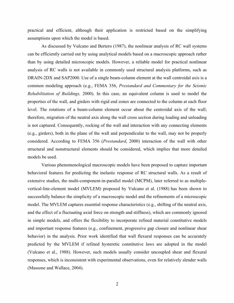
practical and efficient, although their application is restricted based on the simplifying
assumptions upon which the model is based.
As discussed by Vulcano and Bertero (1987), the nonlinear analysis of RC wall systems
can be efficiently carried out by using analytical models based on a macroscopic approach rather
than by using detailed microscopic models. However, a reliable model for practical nonlinear
analysis of RC walls is not available in commonly used structural analysis platforms, such as
DRAIN-2DX and SAP2000. Use of a single beam-column element at the wall centroidal axis is a
common modeling approach (e.g., FEMA 356, Prestandard and Commentary for the Seismic
Rehabilitation of Buildings, 2000). In this case, an equivalent column is used to model the
properties of the wall, and girders with rigid end zones are connected to the column at each floor
level. The rotations of a beam-column element occur about the centroidal axis of the wall;
therefore, migration of the neutral axis along the wall cross section during loading and unloading
is not captured. Consequently, rocking of the wall and interaction with any connecting elements
(e.g., girders), both in the plane of the wall and perpendicular to the wall, may not be properly
considered. According to FEMA 356 (Prestandard, 2000) interaction of the wall with other
structural and nonstructural elements should be considered, which implies that more detailed
models be used.
Various phenomenological macroscopic models have been proposed to capture important
behavioral features for predicting the inelastic response of RC structural walls. As a result of
extensive studies, the multi-component-in-parallel model (MCPM), later referred to as multiple-
vertical-line-element model (MVLEM) proposed by Vulcano et al. (1988) has been shown to
successfully balance the simplicity of a macroscopic model and the refinements of a microscopic
model. The MVLEM captures essential response characteristics (e.g., shifting of the neutral axis,
and the effect of a fluctuating axial force on strength and stiffness), which are commonly ignored
in simple models, and offers the flexibility to incorporate refined material constitutive models
and important response features (e.g., confinement, progressive gap closure and nonlinear shear
behavior) in the analysis. Prior work identified that wall flexural responses can be accurately
predicted by the MVLEM if refined hysteretic constitutive laws are adopted in the model
(Vulcano et al., 1988). However, such models usually consider uncoupled shear and flexural
responses, which is inconsistent with experimental observations, even for relatively slender walls
(Massone and Wallace, 2004).

3
1.2 OBJECTIVES AND SCOPE
Although relatively extensive research has been conducted to develop a MVLEM for structural
walls, the MVLEM has not been implemented into widely available computer programs and
limited information is available on the influence of material behavior on predicted responses. As
well, the model has not been sufficiently calibrated with and validated against extensive
experimental data for both global (e.g., wall displacement and rotation) and local (i.e., section
curvature and strain at a point) responses. The reliability of the model in predicting the shear
behavior of walls is questionable and an improved methodology that relates flexural and shear
responses is needed. As well, the model has not been assessed and calibrated for walls with
flanged (e.g., T-shaped) cross sections. According to FEMA 356 (Prestandard, 2000), either a
modified beam-column analogy (Yan and Wallace, 1993) or a multiple-spring approach (as in
the MVLEM) should be used for modeling rectangular walls and wall segments with aspect
(height-to-length) ratios smaller than 2.5, as well as for flanged wall sections with aspect ratios
smaller than 3.5. However, either the MVLEM or a similar multiple-spring model is not
available in most codes. The leading and most recently released structural analysis software used
in the industry for reinforced concrete design applications, “RAM Perform” (RAM International,
2003), uses a fiber-cross-section element for modeling of slender walls; however, the nonlinear
response is represented by simplified ad hoc force-deformation relations (trilinear force-
deformation envelopes and simple hysteresis rules) as opposed to incorporating well-calibrated
material behavior in the model response.
Given the shortcomings noted above, a research project was undertaken at the University
of California, Los Angeles, to investigate and improve the MVLEM for both slender and squat
RC walls, as well as to calibrate and validate it against extensive experimental data. More recent
modifications of the MVLEM (Fischinger et al., 1990; Fajfar and Fischinger, 1990; Fischinger et
al., 1991, 1992) have included implementing simplified force-deformation rules for the model
sub-elements to capture the behavior observed in experimental results; however, the resulting
models are tied to somewhat arbitrary force-deformation parameters, the selection of which was
based on engineering judgment. An alternative approach is adopted here, where up-to-date and
state-of-the-art cyclic constitutive relations for concrete and reinforcing steel are adopted to track
the nonlinear response at both the global and local levels, versus the use of simplified (ad hoc)
force-deformation rules as done in prior studies. Therefore, the MVLEM implemented in this

4
study relates the predicted response directly to material behavior without incorporating any
additional empirical relations. This allows the designer to relate analytical responses directly to
physical material behavior and provides a more robust modeling approach, where model
improvements result from improvement in constitutive models, and refinement in the spatial
resolution of the discrete model. The analytical model, as adopted here, is based on a fiber
modeling approach, which is the current state-of-the-art tool for modeling slender reinforced
concrete members.
Upon implementation of updated and refined cyclic constitutive relations in the analytical
model, the effectiveness of the MVLEM for modeling and simulating the inelastic response of
reinforced concrete structural walls was demonstrated. Variation of model and material
parameters was investigated to identify the sensitivity of analytically predicted global and local
wall responses to changes in these parameters as well as to identify which parameters require the
greatest care with respect to calibration.
Once the model was developed, the accuracy and limitations of the model were assessed
by comparing responses predicted with the model to responses obtained from experimental
studies of slender walls for rectangular and T-shaped cross sections. Appropriate nonlinear
analysis strategies were adopted in order to compare model results with results of the drift-
controlled cyclic tests subjected to prescribed lateral displacement histories. The analytical
model was subjected to the same conditions experienced during testing (e.g., loading protocol,
fluctuations in applied axial load). Wall test results were processed and filtered to allow for a
direct and refined comparison of the experimental results with the response prediction of the
analytical model. The correlation of the experimental and analytical results was investigated in
detail, at various response levels and locations (e.g., forces, displacements, rotations, and strains
in steel and concrete).
Furthermore, improved nonlinear shear behavior was incorporated in the analytical
modeling approach. The formulation of the original fiber-based model was extended to simulate
the observed coupling behavior between nonlinear flexural and shear responses in RC walls, via
implementing constitutive RC panel elements into the formulation. Results obtained with the
improved model were compared with test results for both slender wall and short wall specimens.
The formulation of the analytical model proposed and the constitutive material models used in
this study were implemented in the open-source computational platform OpenSees
(“OpenSees”), being developed by the Pacific Earthquake Engineering Research Center.

5
In summary, the objectives of this study are:
1. to develop an improved fiber-based modeling approach for simulating flexural
responses of RC structural walls, by implementing updated and refined constitutive
relations for materials,
2. to adopt nonlinear analysis solution strategies for the analytical model,
3. to investigate the influence of material behavior on the analytical model response, and
to conduct studies to assess the sensitivity of the analytically predicted global and
local wall responses to changes in material and model parameters,
4. to carry out detailed calibration studies of the analytical model and to conduct
comprehensive correlation studies between analytical model results and extensive
experimental results at various response levels and locations,
5. to further improve the modeling methodology, in order to improve the shear response
prediction of the analytical model, considering the coupling of flexural and shear
responses in RC structural walls,
6. to assess effectiveness and accuracy of the analytical model in predicting the
nonlinear responses of both slender and squat reinforced concrete walls, and to arrive
at recommendations upon applications and further improvements of the model,
7. to implement the formulation of the analytical models proposed and the constitutive
material models used in this study into a commonly used structural analysis platform.
1.3 ORGANIZATION
This report is divided into ten chapters. Chapter 2 provides a review of previous research
conducted on the development of the analytical model. Chapter 3 gives a description of the
improved analytical model, as implemented in this study. Chapter 4 describes the hysteretic
constitutive relations for materials incorporated in the analytical model for predicting flexural
responses. Numerical solution strategies adopted to conduct nonlinear analyses using the
analytical model are described in Chapter 5. Chapter 6 provides an examination of analytical
model results and attributes, and also investigates the sensitivity of the model results to material
and model parameters. Chapter 7 provides information on correlation of the analytical model
results with experimental results for wall flexural responses. A description of the experimental
program, detailed information on calibration of the model, and comparisons of model results

6
with extensive experimental data at global and local response levels are presented. Chapter 8
describes the methodology implemented in the fiber-based analytical model to simulate the
observed coupling between flexural and shear wall responses. A detailed description of the
improved analytical model is presented, and analytical model results are compared with test
results for slender and short wall specimens to evaluate the modeling approach. A summary and
conclusions are presented in Chapter 10. Recommendations for model improvements and
extensions are also provided. Chapters 3, 5, 6, and 7 provide information mostly on the flexural
response modeling aspects of this analytical study, whereas coupled shear and flexural response
modeling aspects are presented in Chapters 8 and 9.

2 Related Research
Various analytical models have been proposed for predicting the inelastic response of RC
structural walls. A common modeling approach for wall hysteretic behavior uses a beam-column
element at the wall centroidal axis with rigid links on beam girders. Commonly a one-component
beam-column element model is adopted. This model consists of an elastic flexural element with
a nonlinear rotational spring at each end to account for the inelastic behavior of critical regions
(Fig. 2.1); the fixed-end rotation at any connection interface can be taken into account by a
further nonlinear rotational spring. To more realistically model walls, improvements, such as
multiple spring representation (Takayanagi and Schnobrich, 1976), varying inelastic zones
(Keshavarzian and Schnobrich, 1984), and specific inelastic shear behavior (Aristizabal, 1983)
have been introduced into simple beam-column elements. However, inelastic response of
structural walls subjected to horizontal loads is dominated by large tensile strains and fixed end
rotation due to bond slip effects, associated with shifting of the neutral axis. This feature cannot
be directly modeled by a beam-column element model, which assumes that rotations occur
around points on the centroidal axis of the wall. Therefore, the beam-column element disregards
important features of the experimentally observed behavior (Fig. 2.2), including variation of the
neutral axis of the wall cross section, rocking of the wall, and interaction with the frame
members connected to the wall (Kabeyasawa et al., 1983).
Following a full-scale test on a seven-story RC frame-wall building in Tsubaka, Japan,
Kabeyasawa et al. (1983) proposed a new macroscopic three-vertical-line-element model
(TVLEM), to account for experimentally observed behavior that could not be captured using an
equivalent beam-column model. The wall member was idealized as three vertical line elements
with infinitely rigid beams at the top and bottom (floor) levels (Fig. 2.3); two outside truss
elements represented the axial stiffness of the boundary columns, while the central element was a
one-component model with vertical, horizontal, and rotational springs concentrated at the base.

8
(a) Beam-column element (b) Model configuration
Fig. 2.1 Beam-column element model
(a) Beam-column element model (b) Observed Behavior
Fig. 2.2 Wall rocking and effect of neutral axis shift on vertical displacements
The axial-stiffness hysteresis model (ASHM), defined by the rules shown in Figure 2.4,
was used to describe the axial force–deformation relation of the three vertical line elements of
the wall model. An origin-oriented-hysteresis model (OOHM) was used for both the rotational
and horizontal springs at the base of the central vertical element (Fig. 2.5). The stiffness
properties of the rotational spring were defined by referring to the wall area bounded by the inner
Rigid End Zones
Nonlinear Rotational Springs
Nonlinear Axial Spring
Linear Elastic Element
Δ Δ
ΦΦ
Beams
Wall
Rigid End Zones

9
faces of the two boundary columns (central panel only); therefore, displacement compatibility
with the boundary columns was not enforced. Shear stiffness degradation was incorporated, but
was assumed to be independent of the axial force and bending moment.
Fig. 2.3 Three-vertical-line-element model (TVLEM)
Fig. 2.4 Axial-stiffness hysteresis model (ASHM) (Kabeyasawa et al., 1983)
Level m
Rigid Beam
Level m-1
Kv
K1
K2
KH
Kφ
h
Rigid Beam
Δφm
Δvm
l
Δwm
(Dx, Fm-Fy)
FORCE, F (tension)
DEFORMATION, D (extension)
Y (Dyt, Fy)
M (Dm, Fm) Kr
Kt
Kc
Kc
Kh
Y’ (Dyc, -Fy)
P (Dp, Fp)
Y’’ (2Dyc, -2Fy)
Kr = Kc (Dyt/Dm)α
Dp = Dyc + β(Dx-Dyc)
α , β = constants

10
Fig. 2.5 Origin-oriented hysteresis model (OOHM) (Kabeyasawa et al., 1983)
Although the model accounted for fluctuation of the neutral axis of the wall and the
interaction of the wall with surrounding frame elements (i.e., often referred to as “outrigging”),
and predicted global responses (top displacement, base shear, axial deformation at wall
boundaries, rotation at beam ends) compared favorably with experimental responses, general
application of this model was limited by difficulties in defining the properties and physical
representation of the springs representing the panel, and the incompatibility that exists between
the panel and the boundary columns.
Vulcano and Bertero (1986) modified the TVLEM by replacing the axial-stiffness
hysteresis model (ASHM) with the two-axial-element-in-series model (AESM) shown in Figure
2.6. Element 1 in Figure 2.6 was a one-component model to represent the overall axial stiffness
of the column segments in which the bond is still active, while element 2 in Figure 2.6 is a two-
component model to represent the axial stiffness of the remaining segments of steel (S) and
cracked concrete (C) for which the bond has almost completely deteriorated. The AESM was
intended to idealize the main features of the actual hysteretic behavior of the materials and their
interaction (yielding and hardening of the steel, concrete cracking, contact stresses, bond
degradation, etc.). Even though refined constitutive laws could have been assumed for describing
the hysteretic behavior of the materials and their interaction, very simple assumptions (i.e.,
linearly elastic behavior for element 1, and bilinear behavior with strain hardening and linearly
elastic behavior in compression neglecting tensile strength, respectively, for steel and concrete
components of the element 2) were made in order to assess the effectiveness and the reliability of
FORCE
DISPLACEMENT
Cracking, C
Yield, Y
C’
Y’
1
2
3

11
the proposed model. The axial force–deformation relation generated by AESM is shown in
Figure 2.7. The origin-oriented hysteresis model (OOHM) was again used for the rotational and
the shear spring at the wall centerline.
Fig. 2.6 Axial-element-in-series model (AESM) (Vulcano and Bertero, 1986)
Fig. 2.7 Axial force–deformation relation of AESM
λh
(steel) EsAs
(concrete) EcAc
EcAc + EsAs
F, D
element 1
element 2
h
(1-λ)h
wc (crack width)
DEFORMATION, D
yielding in tension
Kh
crack closure (wc = 0)
Kc
Kr = Kt
Kt
FORCE, F
yielding in compression
1 + ε EcAc/EsAs
Kc
Kh = 1 + ε 1 + EcAc/EsAs
r
- 1
Kc
r = steel strain hardening ratio ε = constant
12
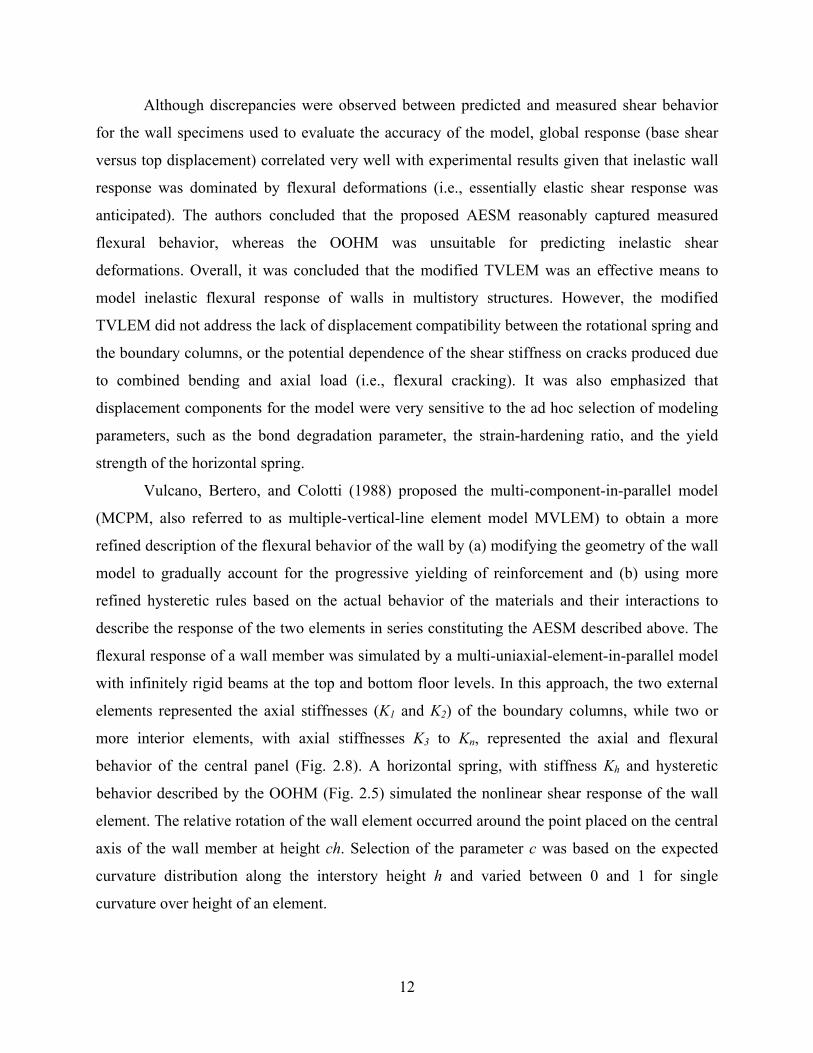
Although discrepancies were observed between predicted and measured shear behavior
for the wall specimens used to evaluate the accuracy of the model, global response (base shear
versus top displacement) correlated very well with experimental results given that inelastic wall
response was dominated by flexural deformations (i.e., essentially elastic shear response was
anticipated). The authors concluded that the proposed AESM reasonably captured measured
flexural behavior, whereas the OOHM was unsuitable for predicting inelastic shear
deformations. Overall, it was concluded that the modified TVLEM was an effective means to
model inelastic flexural response of walls in multistory structures. However, the modified
TVLEM did not address the lack of displacement compatibility between the rotational spring and
the boundary columns, or the potential dependence of the shear stiffness on cracks produced due
to combined bending and axial load (i.e., flexural cracking). It was also emphasized that
displacement components for the model were very sensitive to the ad hoc selection of modeling
parameters, such as the bond degradation parameter, the strain-hardening ratio, and the yield
strength of the horizontal spring.
Vulcano, Bertero, and Colotti (1988) proposed the multi-component-in-parallel model
(MCPM, also referred to as multiple-vertical-line element model MVLEM) to obtain a more
refined description of the flexural behavior of the wall by (a) modifying the geometry of the wall
model to gradually account for the progressive yielding of reinforcement and (b) using more
refined hysteretic rules based on the actual behavior of the materials and their interactions to
describe the response of the two elements in series constituting the AESM described above. The
flexural response of a wall member was simulated by a multi-uniaxial-element-in-parallel model
with infinitely rigid beams at the top and bottom floor levels. In this approach, the two external
elements represented the axial stiffnesses (K1 and K2) of the boundary columns, while two or
more interior elements, with axial stiffnesses K3 to Kn, represented the axial and flexural
behavior of the central panel (Fig. 2.8). A horizontal spring, with stiffness Kh and hysteretic
behavior described by the OOHM (Fig. 2.5) simulated the nonlinear shear response of the wall
element. The relative rotation of the wall element occurred around the point placed on the central
axis of the wall member at height ch. Selection of the parameter c was based on the expected
curvature distribution along the interstory height h and varied between 0 and 1 for single
curvature over height of an element.

13
Fig. 2.8 Multiple-vertical-line-element-model (Vulcano et al., 1988)
A modified version of the AESM was proposed by the authors to describe the response of the
uniaxial vertical elements (Fig. 2.9). Analogous to the original AESM, the two elements in series
represented the axial stiffness of the column segments in which the bond remained active
(element 1) and those segments for which the bond stresses were negligible (element 2). Unlike
the original AESM, element 1 consisted of two parallel components to account for the
mechanical behavior of the uncracked and cracked concrete (C) and the reinforcement (S). A
dimensionless parameter λ was introduced to define the relative length of the two elements
(representing cracked and uncracked concrete) to account for tension stiffening.
Fig. 2.9 Modified axial-element-in-series model (Vulcano et al., 1988)
K2 K3 Kn
h
l/2
Rigid Beam (Level m)
Δwm = wm - wm-1
l/2
Rigid Beam (Level m-1)
ch
Kh
x
Δvm = vm - vm-1
Δφm = φm - φm-1
element 1
element 2
h
(1-λ)h
λh
F, D
Steel
Concrete (uncracked)
Steel
Concrete (cracked)

14
Relatively refined constitutive laws were adopted to idealize the hysteretic behavior of
the materials. The stress-strain relation proposed by Menegotto and Pinto (1973) was adopted by
the authors to describe the hysteretic response of reinforcing steel (Fig. 2.10). The stress-strain
relation proposed by Colotti and Vulcano (1987) was adopted for uncracked concrete (Fig.
2.11(a)). The stress-strain relation proposed by Bolong et al. (1980), which accounts for the
contact stresses due to the progressive opening and closing of cracks, was used to model cracked
concrete (Fig. 2.11(b)). Under monotonic tensile loading, the tension-stiffening effect was
incorporated by manipulating the value of the dimensionless parameter λ such that the tensile
stiffness of the uniaxial model in Figure 2.9 would be equal to the actual tensile stiffness of the
uniaxial RC member as:
( )m
sss
sssscct hAE
AEh
AEAEh
εελλ =
⎭⎬⎫
⎩⎨⎧
++
−−1
1 (1.1)
where cct AE and ss AE are the axial stiffnesses in tension of the concrete and of the
reinforcement, respectively, and ms εε is the ratio of the steel strain in a cracked section to the
current average strain for the overall member, evaluated by the empirical law proposed by
Rizkalla and Hwang (1984). Under cyclic loading, the value of λ was based on the peak tensile
strain obtained in prior cycles, and remained constant during loading and unloading unless the
peak tensile strain obtained in prior cycles was exceeded.
Fig. 2.10 Constitutive law adopted in original MVLEM for reinforcing steel
1
σ/σy
ε/εy
ξ1
ξ4
ξ3
ξ2
1
1
2
3
4
R0
R(ξ1)
R(ξ3) R(ξ1)
R(ξ4)
arctan (b)

15
(a) Uncracked concrete (Colotti and Vulcano, 1987)
(b) Cracked concrete (Bolong et al., 1980)
Fig. 2.11 Constitutive laws adopted in original MVLEM for concrete
Comparison with experimental results indicated that, with the refined constitutive laws
adopted, a reliable prediction of inelastic flexural response (base shear versus top displacement)
was obtained, even with relatively few uniaxial elements ( 4=n ). In addition, greater accuracy
was obtained by calibrating the parameter c defining the relative rotation center of the generic
wall member, versus using more uniaxial elements. Therefore the authors concluded that the use
of relatively simple constitutive laws for the materials and including tension stiffening provided
a reliable model well suited for practical nonlinear analysis of multistory RC frame-wall
structural systems. The OOHM used to model nonlinear shear behavior still had shortcomings,
and the relative contribution of shear and flexural displacement components was difficult to
predict and varied significantly with the selection of model parameters.
As mentioned above, the accuracy in predicting the flexural response of the wall by the
multiple-vertical-line-element model (MVLEM) was very good when the constitutive laws in
Figures 2.10–2.11 were adopted for the modified AESM components in Figure 2.9, even where
relatively few uniaxial elements are used. However, because the constitutive laws incorporated
εu
0.3 ε0
σ0
ε
(εi , σi)
ε0
ε1
arctan (Ec)
εu
σ
0.3 ε0
ε
σ0
ε0
εp
ε1
(εi , σi)
σn
p
εr
-|εt| max

16
into the model are relatively sophisticated, to improve the effectiveness of the MVLEM without
compromising accuracy, the use of simplified constitutive laws was investigated.
Fischinger et al. (1990) introduced simplified hysteretic rules to describe the response of
both the vertical and horizontal springs (Fig. 2.12). The so-called modified MVLEM also proved
to be very efficient in prediction of the cyclic response of a RC structural wall; however, the
model included numerous parameters, some of which could be easily be defined, while others
were difficult to define (in particular, the parameters of inelastic shear behavior and the
parameter β in Figure 2.12(a) defining the fatness of the hysteresis loops). Therefore, the
analytical results obtained using the modified MVLEM were based on somewhat arbitrary force-
deformation parameters, the selection of which depended on engineering judgment.
(a) Vertical springs
(b) Horizontal spring
Fig. 2.12 Force-deformation relations adopted in modified MVLEM
Dmax
FORCE, F
DEFORMATION, D
Fy
αFy
FI
βFy
Dy
λ (Dmax - Dy)
k’’ = k’ (Dy/Dmax)δ
α , β , δ = constants
k’ k’’
k’’
FORCE, Q
DISPLACEMENT, U
Qy
f Qy
Pinchingf = constant

17
A further variant of the modified MVLEM was applied in a study by Fajfar and
Fischinger (1990), who, in order to reduce the uncertainty in the assumption of a suitable value
for the parameter c, used a stack of a larger number of model elements placed one upon the
other. A later study conducted by Fischinger, Vidic, and Fajfar (1992), showed that the modified
MVLEM was well suited for modeling coupled wall response. It was also emphasized that better
models are needed to account for cases with significant inelastic shear deformations as well as
for cases with high levels of axial force, where the influence of transverse reinforcement
(confinement on the nonlinear behavior of the vertical springs (in compression)) was found to be
an important consideration.
A more recent study by Kabeyasawa (1997) proposed a modification to the original
three-vertical-line-element model (TVLEM) in order to improve the prediction of the overall
(shear and flexural) behavior of RC structural walls for both monotonic and reversed cyclic
loading. The primary modification of the TVLEM involved substituting a two-dimensional
nonlinear panel element for the vertical, horizontal, and rotational springs at the wall centerline
(Fig. 2.13). Comparisons with experimental results indicated that both the TVLEM and the new
panel-wall macro element (PWME) could be used to accurately model coupled walls under
monotonic and reversed cyclic lateral loading and axial load. However, both models were found
to be unstable for cases with high axial load and significant cyclic nonlinear shear deformations.
Simulation of the concrete shear response as a function of axial load appeared to be a weak point
for the PWME model.
Panel RC Element
Gauss Points
Rigid Beam
Axial Springs
Bending Spring
Shear Spring
Level m
Level m-1
Boundary Column
(a) Original model layout (b) Modified model layout
Fig. 2.13 Modification of TVLEM (Kabeyasawa et al., 1997)
The MVLEM was also modified using a similar approach to incorporate coupling
between axial and shear components of RC wall response. Colotti (1993) modified the MVLEM

18
model by substituting the horizontal spring of each MVLE with a single two-dimensional
nonlinear panel element in the MVLEM. In general, the results obtained using this model were
more accurate compared with prior macro-models that use ad hoc shear force–deformation
relations, although the relative contributions of shear and flexural deformations on wall
displacements computed using this model showed discrepancies with experimental data. Shear
deformations predicted by the model were, in some cases, approximately 20% greater than
measured values. The model retained the inability to incorporate interaction between shear and
flexure, as it considered coupling between shear and axial responses only, which was shown
experimentally by Massone and Wallace (2004) to be unrealistic.
However, various approaches to consider the coupling between flexural and shear
response components have been reported in the literature. One approach, by Takayanagi et al.
(1979), involves using a shear force–displacement relation having a yield point (force at shear
yield yielding) based on the lateral load to reach flexural yielding, so that flexural and yielding
behavior are initiated simultaneously during loading. Another common approach involves using
the finite element formulation together with constitutive reinforced concrete panel elements (e.g.,
modified compression field theory (MCFT, Vecchio and Collins, 1986); rotating-angle softened-
truss model (RA-STM, Belarbi and Hsu, 1994; Pang and Hsu, 1995); disturbed stress field model
(DSFM, Vecchio, 2000)). Even so, the direct application of the finite element method may
provide relatively accurate results,
A simplification of a fully implemented finite element formulation with constitutive
reinforced concrete panel elements is a one-story macro-element based on relatively simple
uniaxial constitutive material relations for modeling flexural response components, together with
a shear force versus displacement relation coupled with the axial load on the element, as
proposed by Colotti (1993). However, as mentioned in the previous paragraph, this methodology
incorporates coupling of shear and axial response components only, whereas axial-shear-flexure
interaction is not considered. One way to address this limitation is to adopt a sectional analysis
approach, by dividing the one-story macro-element into vertical segments (e.g., uniaxial
elements in the MVLEM), with axial-shear coupling incorporated in each segment, so as to attain
shear-flexure coupling, since the axial responses of the vertical segments constitute the flexural
response of the element (Bonacci, 1994). An approach based on adopting this idea for a standard
displacement-based element with a cross-sectional multilayer or fiber discretization was

19
proposed by Petrangeli et al. (1999a), and provided reasonably good response predictions for
slender elements (Petrangeli, 1999b).
In this study, the multiple-vertical-line-element model (MVLEM) was improved by
adopting refined constitutive relations for materials, and detailed calibration correlation studies
were conducted to investigate the effectiveness of the model in predicting flexural responses of
walls under cyclic loading. A description of the flexural model, as adopted in this study, is
presented in the following chapter. The MVLEM was further modified in this study, using an
approach similar to that of Petrangeli et al. (1999a), to incorporate interaction between flexure
and shear components of wall response. A description of the shear-flexure interaction modeling
methodology adopted is presented in the Chapter 8.
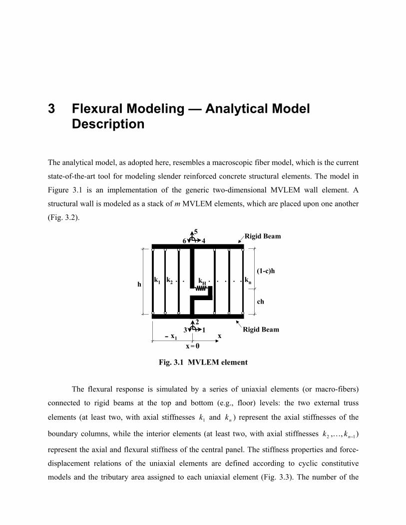
3 Flexural Modeling — Analytical Model Description
The analytical model, as adopted here, resembles a macroscopic fiber model, which is the current
state-of-the-art tool for modeling slender reinforced concrete structural elements. The model in
Figure 3.1 is an implementation of the generic two-dimensional MVLEM wall element. A
structural wall is modeled as a stack of m MVLEM elements, which are placed upon one another
(Fig. 3.2).
Fig. 3.1 MVLEM element
The flexural response is simulated by a series of uniaxial elements (or macro-fibers)
connected to rigid beams at the top and bottom (e.g., floor) levels: the two external truss
elements (at least two, with axial stiffnesses 1k and nk ) represent the axial stiffnesses of the
boundary columns, while the interior elements (at least two, with axial stiffnesses 2k ,…, 1−nk )
represent the axial and flexural stiffness of the central panel. The stiffness properties and force-
displacement relations of the uniaxial elements are defined according to cyclic constitutive
models and the tributary area assigned to each uniaxial element (Fig. 3.3). The number of the
-
h
(1-c)h
ch
1 2
3
4 5
6 Rigid Beam
Rigid Beam x 1 x
k 1 k 2 k nk H. . . . . . .
x = 0

22
uniaxial elements (n) can be increased to obtain a more refined description of the wall cross
section.
RC WALL WALL MODEL
1
2
m
. . . . .
Fig. 3.2 Modeling of a wall with MVLEM
1k 32k k4k 5k 6k 87k k
Fig. 3.3 Tributary area assignment
The relative rotation between the top and bottom faces of the wall element occurs around
the point placed on the central axis of the element at height ch (Fig. 3.4). Rotations and resulting
transverse displacements are calculated based on the wall curvature, derived from section and
material properties, corresponding to the bending moment at height ch of each element (Fig. 3.4).
MOMENT
ch
(1-c)hΦ = φh
CURVATURE
φ
Δ = Φ(1-c)h
Φ
Fig. 3.4 Rotations and displacements of MVLEM element

23
A suitable value of the parameter c is based on the expected curvature distribution along
the element height h. For example, if moment (curvature) distribution along the height of the
element is constant, using a value of 5.0=c yields “exact” rotations and transverse
displacements for elastic and inelastic behavior. For a triangular distribution of bending moment
over the element height, using 5.0=c yields exact results for rotations in the elastic range but
underestimates displacements. Selection of c becomes important in the inelastic range, where
small changes in moment can yield highly nonlinear distributions of curvature. Consequently,
lower values of c should be used to take into account the nonlinear distribution of curvature
along the height of the wall. A value of 4.0=c was recommended by Vulcano et al. (1988)
based on comparison of the model response with experimental results. Stacking more elements
along the wall height, especially in the regions where inelastic deformations are expected, will
result in smaller variations in the moment and curvature along the height of each element, thus
improving analytical accuracy (Fischinger et al., 1992).
A horizontal spring placed at the height ch, with a nonlinear hysteretic force-deformation
behavior following an origin-oriented hysteresis model (OOHM) (Kabeyasawa et al., 1983) was
originally suggested by Vulcano et al. (1988) to simulate the shear response of the wall element.
A trilinear force-displacement backbone curve with pre-cracked, post-cracked and post-yield
shear stiffness values of the wall cross section was adopted to define the stiffness and force-
deformation properties of the horizontal spring in each wall element. Unloading and reloading
occurred along straight lines passing through the origin (Fig. 3.5). The OOHM was proven to be
unsuitable by Vulcano and Bertero (1987) for an accurate idealization of the shear hysteretic
behavior especially when high shear stresses are expected. Improved predictions of wall shear
response likely require consideration of the interaction between shear and flexure responses.
The first part of this study focuses on modeling and simulation of the flexural responses
of slender RC walls, thus a linear elastic force-deformation behavior was adopted for the
horizontal “shear” spring. For the present model, flexural and shear modes of deformation of the
wall member are uncoupled (i.e., flexural deformations do not affect shear strength or
deformation), and the horizontal shear displacement at the top of the element does not depend on
c (Fig. 3.6). However, the second part of this study involves extending the formulation of present
model was extended to simulate coupled shear and flexural wall responses, as described in
Chapters 8 and 9.

24
Displacement
Forc
eO
Cracking
Yield
Fig. 3.5 Origin-oriented hysteresis model for horizontal shear spring
Flexure ShearDeformation
Fig. 3.6 Uncoupling of modes of deformation of MVLEM element
A single two-dimensional MVLE has six global degrees of freedom, three of each located
at the center of the rigid top and bottom beams (Fig. 3.1). The strain level in each uniaxial
element is obtained from the element displacement components (translations and rotations) at the
six nodal degrees of freedom using the plane-sections-remain-plane kinematic assumption.
Accordingly, if [ ]δ is a vector that represents the displacement components at the six nodal
degrees of freedom of each MVLE (Fig. 3.1):

25
[ ]
⎥⎥⎥⎥⎥⎥⎥⎥
⎦
⎤
⎢⎢⎢⎢⎢⎢⎢⎢
⎣
⎡
=
6
5
4
3
2
1
δδδδδδ
δ (3.1)
then, the resulting deformations of the uniaxial elements are obtained as:
[ ] [ ] [ ]δ⋅= au (3.2)
where [ ]u denotes the axial deformations of the uniaxial elements:
[ ]
⎥⎥⎥⎥⎥⎥⎥⎥⎥⎥⎥
⎦
⎤
⎢⎢⎢⎢⎢⎢⎢⎢⎢⎢⎢
⎣
⎡
=
n
i
u
u
uu
u
.
.
.
.2
1
(3.3)
and [ ]a is the geometric transformation matrix that converts the displacement
components at the nodal degrees of freedom to uniaxial element deformations:
[ ]
⎥⎥⎥⎥⎥⎥⎥⎥⎥⎥⎥
⎦
⎤
⎢⎢⎢⎢⎢⎢⎢⎢⎢⎢⎢
⎣
⎡
−
−−
−−−−
=
nn
ii
xx
xx
xxxx
a
0000............
1010............
10101010
22
11
(3.4)
The average axial strain in each uniaxial element ( )iε can then be calculated by simply
dividing the axial deformation by the element height, h:
hui
i =ε (3.5)
The average strains in concrete and steel are typically assumed equal (perfect bond)
within each uniaxial element.

26
The deformation in the horizontal shear spring ( )Hu of each MVLE can be similarly
related to the deformation components [ ]δ at the six nodal degrees of freedom as:
[ ] [ ]δTH bu = (3.6)
where the geometric transformation vector [ ]b is defined as:
[ ]
( ) ⎥⎥⎥⎥⎥⎥⎥⎥
⎦
⎤
⎢⎢⎢⎢⎢⎢⎢⎢
⎣
⎡
−−
−−
=
hc
chb
101
01
(3.7)
The stiffness properties and force-deformation relations of the uniaxial elements are
defined according to the uniaxial constitutive relations adopted for the wall materials, (i.e.,
concrete and steel), as well as the tributary area assigned to each uniaxial element. For a
prescribed strain level ( )iε at the i-th uniaxial element, the axial stiffness of the i-th uniaxial
element ( )ik is defined as:
( ) ( ) ( ) ( )h
AEh
AEk isisicic
i += (3.8)
where ( )icE and ( )isE are the material tangent moduli (strain derivatives of the adopted
constitutive stress-strain relations), respectively for concrete and steel, at the prescribed strain
level ( )iε ; ( )icA and ( )isA are the tributary concrete and steel areas assigned to the uniaxial
element, and h is the element height. The axial force in the i-th uniaxial element ( )if is defined
similarly as:
( ) ( ) ( ) ( )isisicici AAf σσ += (3.9)
where ( )icσ and ( )isσ are the uniaxial stresses, respectively, for concrete and steel,
obtained from the implemented constitutive relations at the prescribed strain ( )iε . The stiffness
of the horizontal shear spring ( )Hk and the force in the horizontal spring ( )Hf for a prescribed
spring deformation ( )Hu are derived from the force-deformation relation adopted in the model
for shear (e.g., origin-oriented-hysteresis relation or linear elastic relation).
Consequently, for a specified set of displacement components at the six nodal degrees of
freedom of a generic wall element, if Hk is the stiffness of the horizontal spring, ik is the

27
stiffness of the i-th uniaxial element, and ix is the distance of the i-th uniaxial element to the
central axis of the element, the stiffness matrix of the element relative to the six degrees of
freedom is obtained as:
[ ] [ ] [ ] [ ]ββ ⋅⋅= KK Te (3.10)
where [ ]β denotes the geometric transformation matrix converting the element degrees
of freedom to the element deformations of extension, relative rotation at the bottom and relative
rotation at the top of each wall element (Fig. 3.7):
[ ]⎥⎥⎥
⎦
⎤
⎢⎢⎢
⎣
⎡
−−
−=
10/100/100/110/1010010
hhhhβ (3.11)
and
[ ]
⎥⎥⎥⎥⎥⎥⎥
⎦
⎤
⎢⎢⎢⎢⎢⎢⎢
⎣
⎡
+−
−−+
−
=
∑
∑∑
∑∑∑
=
==
===
n
iiiH
n
iiiH
n
iiiH
n
iii
n
iii
n
ii
xkhcksymm
xkhcckxkhck
xkxkk
K
1
222
1
22
1
222
111
)1(.
)1( (3.12)
is the element stiffness matrix relative to the three pure deformation degrees of freedom
shown in Figure 3.7.
Extension Relative Rotation at the Bottom
Relative Rotation at the Top
Fig. 3.7 Element deformations of MVLEM element (Vulcano et al., 1988)

28
Similarly, if Hf is the force in the horizontal spring, and if is the force in the i-th
uniaxial element, the internal (resisting) force vector of the wall element relative to the six
degrees of freedom is obtained from equilibrium as:
[ ]
( )⎥⎥⎥⎥⎥⎥⎥⎥⎥⎥⎥⎥⎥⎥⎥
⎦
⎤
⎢⎢⎢⎢⎢⎢⎢⎢⎢⎢⎢⎢⎢⎢⎢
⎣
⎡
+−−
−
−−
−
=
∑
∑
∑
∑
=
=
=
=
n
iiiH
n
ii
H
n
iiiH
n
ii
H
xfhcf
f
f
xfchf
f
f
F
1
1
1
1
int
1
(3.13)
Overall, the MVLEM implemented in this study is an efficient approach to relate the
predicted wall flexural response directly to uniaxial material behavior without incorporating any
additional empirical relations. Its physical concept is clear, and the required computational effort
is reasonable. The primary simplification of the model involves applying the plane-sections-
remain-plane kinematic assumption to calculate the average strain level within each of the
uniaxial sub-elements. The only parameters associated with the wall model are the number of
uniaxial elements used along the length of the wall cross section (n), the number of MVLEM
elements stacked on top of each other along the height of the wall (m), and the parameter
defining the location of the center of rotation along the height of each MVLEM element (c). The
number of the uniaxial elements (n) and the MVLEM elements (m) can be increased to obtain a
more refined description of the wall cross geometry and a more accurate representation of the
flexural response. In addition to the model parameters, parameters associated with the material
constitutive relations govern the analytical response predictions. Details of the constitutive
models adopted in this study for steel and concrete are described in the following chapter.
4 Flexural Modeling — Material Constitutive Models
The MVLEM implemented in this study relates the predicted flexural response directly to
uniaxial material behavior without incorporating any additional empirical relations. The
approach adopted here involves implementing state-of-the-art cyclic constitutive relations for
concrete and reinforcing steel to track the nonlinear response of the model sub-elements, versus
the use of simplified (ad hoc) force-deformation rules as done in prior studies (Fischinger et al.,
1990; Fajfar and Fischinger, 1990; Fischinger et al., 1991, 1992). The stiffness and force-
deformation properties of the model sub-elements are derived from uniaxial stress-strain
behavior of materials; therefore, responses obtained using the present wall model are governed
by the properties and parameters of the adopted material constitutive relations. Details of the
uniaxial hysteretic constitutive models used in this study for steel and concrete are described in
the following sections.
4.1 CONSTITUTIVE MODEL FOR REINFORCEMENT
The uniaxial constitutive stress-strain relation implemented in the wall model for reinforcing
steel is the well-known nonlinear hysteretic model of Menegotto and Pinto (1973), as extended
by Filippou et al. (1983) to include isotropic strain-hardening effects. The model is
computationally efficient and capable of reproducing experimental results with accuracy. The
relation is in the form of curved transitions (Fig. 4.1), each from a straight-line asymptote with
slope 0E (modulus of elasticity) to another straight-line asymptote with slope 01 bEE = (yield
modulus) where the parameter b is the strain-hardening ratio. The curvature of the transition
curve between the two asymptotes is governed by a cyclic curvature parameter R , which permits
the Bauschinger effect to be represented.

30
The uniaxial hysteretic stress-strain (σ - )ε relation of Menegotto and Pinto (1973) takes
the form:
( )( ) RR
b /1*
***
1b-1
εεεσ
++= (4.1)
where
r
r
εεεεξ
−−
=0
* (4.2)
and
r
r
σσσσσ
−−=
0
* (4.3)
Equation (4.1) represents the curved transition from the elastic asymptote with slope 0E
to the yield asymptote with slope 01 bEE = (Fig. 4.1). Parameters rσ and rε are the stress and
strain at the point of strain reversal, which also forms the origin of the asymptote with slope 0E .
Parameters 0σ and 0ε are the stress and strain at the point of intersection of the two asymptotes.
Parameter b is the strain-hardening ratio, that is the ratio between the slopes 1E and 0E , and R
is the parameter that influences the curvature of the transition curve between the two asymptotes
(and thus permits the Bauschinger effect to be represented). As indicated in Figure 4.1, the strain
and stress pairs ( )rr σε , and ( )00 ,σε are updated after each strain reversal.
The tangent modulus ( )tE of the stress-strain relation is obtained by differentiating the
equations above, and is given by the following expression:
*
*
0
0
εσ
εεσσ
εσ
dd
ddE
r
rt ⎟⎟
⎠
⎞⎜⎜⎝
⎛−−== (4.4)
where
( ) ⎥⎦
⎤⎢⎣
⎡+
−⎥⎥⎦
⎤
⎢⎢⎣
⎡
+−+= R
R
RR
bbdd
*
*
/1** 11
11
*
εε
εεσ (4.5)

31
-0.01 -0.005 0 0.005 0.01 0.015 0.02
Strain, ε
-600
-400
-200
0
200
400
600
Stre
ss, σ
(M
Pa)
εy
E0
E1= bE0(εr
1,σr1)
(εr2,σr
2)(ε0
1,σ01)
(ε02,σ0
2) σy
σ*= b ε*+ (1-b) ε*
(1 + ε* R )1/ R
ε* = ε - εr
ε0 - εr
σ*= σ - σr
σ0 - σr
1
1
Fig. 4.1 Constitutive model for steel (Menegotto and Pinto, 1973)
The curvature parameter R is dependent on the absolute strain difference between the
current asymptote intersection point and the previous maximum or minimum strain reversal point
(Fig. 4.2) depending on whether the current strain is increasing or decreasing, respectively. The
expression for R takes the form suggested by Menegotto and Pinto:
ξ
ξ+
−=2
10 a
aRR (4.6)
where 0R is the value assigned to the parameter R for initial (or monotonic) loading, and
1a and 2a are experimentally determined parameters that represent the degradation of the
curvature within subsequent cycles. The absolute strain difference between the current asymptote
intersection point and the previous maximum or minimum strain reversal point is represented by
the parameter ξ (Fig. 4.2), which can be expressed as:
( )y
m
εεεξ 0−= (4.7)
where mε is the maximum or minimum strain, at the previous point of strain reversal,
depending on whether the current strain is increasing or decreasing, respectively. Parameter 0ε
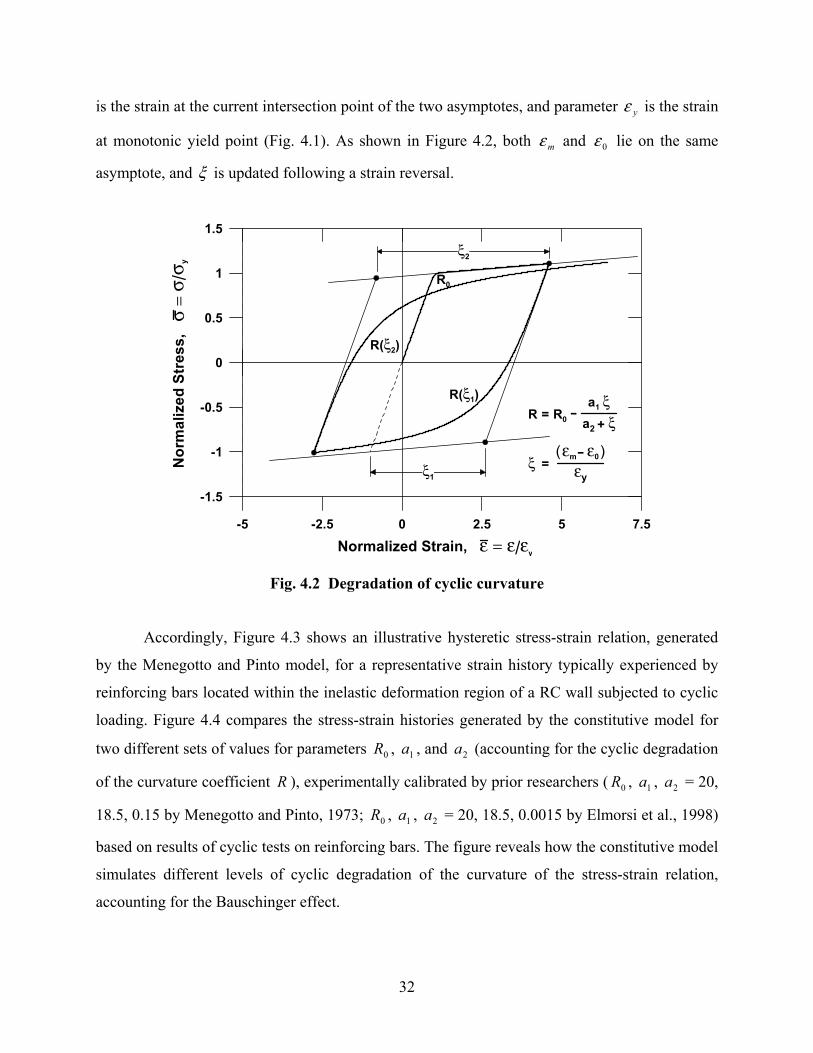
32
is the strain at the current intersection point of the two asymptotes, and parameter yε is the strain
at monotonic yield point (Fig. 4.1). As shown in Figure 4.2, both mε and 0ε lie on the same
asymptote, and ξ is updated following a strain reversal.
-5 -2.5 0 2.5 5 7.5
Normalized Strain, ε = ε/εy
-1.5
-1
-0.5
0
0.5
1
1.5
Nor
mal
ized
Str
ess,
σ
= σ /
σ y ξ2
ξ1
R0
R(ξ1)
R(ξ2)
R = R0 - a1 ξ
a2 + ξ
ξ = ( εm - ε0
)εyεy
Fig. 4.2 Degradation of cyclic curvature
Accordingly, Figure 4.3 shows an illustrative hysteretic stress-strain relation, generated
by the Menegotto and Pinto model, for a representative strain history typically experienced by
reinforcing bars located within the inelastic deformation region of a RC wall subjected to cyclic
loading. Figure 4.4 compares the stress-strain histories generated by the constitutive model for
two different sets of values for parameters 0R , 1a , and 2a (accounting for the cyclic degradation
of the curvature coefficient R ), experimentally calibrated by prior researchers ( 0R , 1a , 2a = 20,
18.5, 0.15 by Menegotto and Pinto, 1973; 0R , 1a , 2a = 20, 18.5, 0.0015 by Elmorsi et al., 1998)
based on results of cyclic tests on reinforcing bars. The figure reveals how the constitutive model
simulates different levels of cyclic degradation of the curvature of the stress-strain relation,
accounting for the Bauschinger effect.

33
-0.01 0 0.01 0.02 0.03 0.04 0.05
Strain, ε
-600
-400
-200
0
200
400
600
800
Stre
ss, σ
(M
Pa)
Fig. 4.3 Stress-strain relation generated by Menegotto and Pinto (1973) model
-0.01 0 0.01 0.02 0.03 0.04 0.05
Strain, ε
-600
-400
-200
0
200
400
600
800
Stre
ss, σ
(M
Pa)
R0=20 a1=18.5 a2=0.15R0=20 a1=18.5 a2=0.0015
Fig. 4.4 Sensitivity of stress-strain relation to cyclic curvature parameters
As discussed by Filippou et al. (1983), the effect of isotropic hardening can be important
when modeling the cyclic behavior of reinforcing bars in RC members. The presence of isotropic
strain hardening can have a pronounced effect on the strain developed in the reinforcing bars

34
during crack closure, as illustrated in Figure 4.5. At a stress 1σ , which satisfies equilibrium, the
corresponding strains of the two models in Figure 4.5 (strains 1ε ′ and 1ε ′′ ) are significantly
different.
0 0.01 0.02 0.03 0.04 0.05
Strain, ε
-600
-400
-200
0
200
400
600
800
Stre
ss, σ
(M
Pa)
Initial Yield Asyptote
Shifted Yield Asyptoteσstσ1
ε1' ε 1
"
εmax ε y
Fig. 4.5 Stress shift due to isotropic strain hardening (Filippou et al., 1983)
In order to account for isotropic strain hardening to improve the prediction of the strains
in reinforcing bars in RC members during crack closure, Filippou et al. (1983) proposed a
modification to the original model by Menegotto and Pinto (1973) by introducing a stress shift to
the yield asymptote. The shift is accomplished by moving the initial (or monotonic) yield
asymptote by a stress magnitude, stσ , parallel to its direction (Fig. 4.5). This idea was
introduced by Stanton and McNiven (1979), who imposed both a stress and a strain shift on the
monotonic envelope curve to arrive at a very accurate representation of hysteretic steel behavior
under generalized strain histories. The simplification introduced by Filippou et al., compared to
the model by Stanton and McNiven, involves the assumption that the monotonic envelope can be
approximated by a bilinear curve, which simplifies the yield asymptotes to straight lines. Thus,
the form and simplicity of the original model (Menegotto and Pinto, 1973) was retained, while a
substantial improvement in results was achieved (Filippou et al., 1983).

35
The imposed stress shift of the yield asymptotes ( )stσ depends on several parameters of
strain history. The main parameter suggested in by Stanton and McNiven (1979) was the sum of
the absolute values of plastic strains up to the most recent strain reversal. Because of differences
in the formulation the model used by Filippou et al. (1983), the authors decided to choose the
maximum plastic strain as the main parameter on which the yield asymptote shift depends. The
relation proposed by Filippou et al. takes the form:
⎟⎟⎠
⎞⎜⎜⎝
⎛−= 4
max3 aa
yy
st
εε
σσ
(4.8)
where maxε is the absolute maximum strain at the instant of strain reversal, yε , yσ are,
respectively, the strain and stress at yield, and 3a and 4a are experimentally determined
parameters. Based on test results, Filippou et al. calibrated the parameter values as: 200 =R ,
5.181 =a , 15.02 =a , 01.03 =a , and 74 =a , with the values for the first three parameters
previously suggested by Menegotto and Pinto (1973).
-0.01 0 0.01 0.02 0.03 0.04 0.05
Strain, ε
-600
-400
-200
0
200
400
600
800
Stre
ss, σ
(M
Pa)
Without Isotropic Strain HardeningWith Isotropic Strain Hardening
Fig. 4.6 Effect of isotropic strain hardening on stress-strain relation
To illustrate the effect of the imposed stress shift on a typical stress-strain history for
reinforcing bars, Figure 4.6 compares the analytical results of the model with and without

36
isotropic strain-hardening effects included. Upon implementation of the above relation proposed
by Filippou et al. (1983), the accuracy of the original Menegotto and Pinto (1973) model in
representing experimental results from cyclic tests on reinforcing bars was substantially
improved, particularly within the strain region where gap closure would be expected. At the
same time, the model is almost as simple and computationally efficient as the original model.
The modification proposed by Filippou et al. to the hysteretic model of Menegotto and Pinto,
was therefore implemented in the present wall model to account for the isotropic strain-
hardening effects on reinforcing bars.
4.2 CONSTITUTIVE MODELS FOR CONCRETE
For an accurate and reliable prediction of wall flexural response using a MVLEM as proposed,
an effective and robust hysteretic constitutive model for concrete is needed. The model addresses
important issues such as the hysteretic behavior in both cyclic compression and tension; the
progressive degradation of stiffness of the unloading and reloading curves for increasing values
of strain; and the effects of confinement, tension stiffening, and gradual crack closure. Two
different constitutive models with such capabilities were adopted in this study, the first being
relatively simple and commonly used, and the latter more refined and generalized.
4.2.1 Hysteretic Constitutive Model by Yassin (1994)
Studies on the stress-strain relations of concrete under cyclic loading have been much fewer than
those under monotonic loading. Sinha et al. (1964) and Karsan and Jirsa (1969) have studied the
behavior of plain concrete subjected to repetitions of compressive stress. It was found in these
studies that the envelope for cyclic loading coincided with the stress-strain curve for monotonic
loading. A uniaxial hysteretic model proposed by Yassin (1994), based on the experimental
results from Sinha et al. (1964) and Karsan and Jirsa (1969), is the first of the two constitutive
models for concrete used in this study. The model takes into account concrete damage and
hysteresis, while retaining computational efficiency.
The monotonic envelope curve of the hysteretic model for concrete in compression
follows the monotonic stress-strain relation model of Kent and Park (1971) as extended by Scott,
Park, and Priestley (1982). Even though more accurate and complete monotonic stress-strain

37
models have been published since, the so-called modified Kent and Park model offers a good
balance between simplicity and accuracy, and is widely used.
Strain, εc
Stre
ss, σ
c
( ε0 , Kf c' )
( ε20 , 0.2Kf c' )
Fig. 4.7 Modified Kent and Park model (1982) for concrete in compression
In the modified Kent and Park model (Fig. 4.7), the monotonic concrete stress-strain
( cσ - )cε relation in compression is described by three regions. Adopting the convention that
compression is positive, the three regions are:
Region OA: 0εε ≤c ⎥⎥⎦
⎤
⎢⎢⎣
⎡⎟⎟⎠
⎞⎜⎜⎝
⎛−
⎟⎟
⎠
⎞
⎜⎜
⎝
⎛′=
2
00
2εε
εεσ cc
cc fK (4.9)
Region AB: 200 εεε ≤< c ( )[ ]01 εεσ −−′= ccc ZfK (4.10)
Region BC: 20εε >c cc fK ′= 2.0σ (4.11)
The corresponding tangent moduli ( )tE are given by the following expressions:
0εε ≤c ⎟⎟⎠
⎞⎜⎜⎝
⎛−
′=
00
12
εε
εcc
tfK
E (4.12)
200 εεε ≤< c ct fZKE ′−= (4.13)
20εε >c 0=tE (4.14)
0εε ≤c ⎥⎥⎦
⎤
⎢⎢⎣
⎡⎟⎟⎠
⎞⎜⎜⎝
⎛−
⎟⎟
⎠
⎞
⎜⎜
⎝
⎛′=
2
00
2εε
εεσ cc
cc fK
200 εεε ≤< c ( )[ ]01 εεσ −−′= ccc ZfK
20εε >c cc fK ′= 2.0σ

38
where
K002.00 =ε (4.15)
c
yhs
ff
K′
+=ρ
1 (4.16)
Ksh
ff
Z
hs
c
c 002.075.01000145
29.035.0
−′
+−′
′+=
ρ (4.17)
In the equations above, 0ε is the concrete strain at maximum compressive stress, 20ε is
the concrete strain at 20% of maximum compressive stress, K is a factor that accounts for the
strength increase due to confinement, Z is the strain softening slope, cf ′ is the concrete
compressive cylinder strength (unconfined peak compressive stress) in MPa, yhf is the yield
strength of transverse reinforcement in MPa, sρ is the ratio of the volume of transverse
reinforcement to the volume of concrete core measured to the outside of stirrups, h′ is the width
of concrete core measured to the outside of stirrups, and hs is the center to center spacing of
stirrups or hoop sets.
The hysteretic unloading and reloading rules proposed by Yassin (1994) are a set of
linear stress-strain relations, as shown in Figure 4.8. The figure illustrates that hysteretic
behavior occurs in both compression and tension. Although the compressive and tensile
hysteresis loops are continuous, they are discussed separately for the sake of clarity.
For compression, successive stiffness degradation for both unloading and reloading, for
increasing values of maximum strain, are shown in Figure 4.9. The stiffness degradation is such
that the projections of all reloading lines intersect at a common point R . Point R is determined
by the intersection of the tangent to the monotonic envelope curve at the origin and the
projection of the unloading line from point B, which corresponds to a concrete strength cf ′2.0
(Fig. 4.9). The strain and stress at the intersection point are given by the following expressions:
20
20202.0EEEfK
c
cr −
−′=
εε (4.18)
rcr E εσ = (4.19)
where cE is the tangent modulus of the monotonic envelope curve at the origin, and 20E is the
unloading modulus at point B of the monotonic envelope curve with a compressive stress of
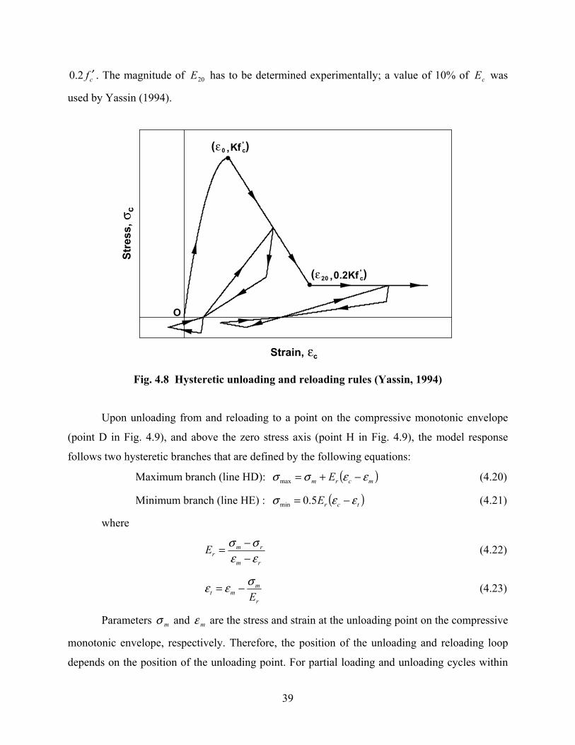
39
cf ′2.0 . The magnitude of 20E has to be determined experimentally; a value of 10% of cE was
used by Yassin (1994).
Strain, εc
Stre
ss, σ
c
O
( ε 0 , Kf c' )
( ε 20 , 0.2Kf c' )
Fig. 4.8 Hysteretic unloading and reloading rules (Yassin, 1994)
Upon unloading from and reloading to a point on the compressive monotonic envelope
(point D in Fig. 4.9), and above the zero stress axis (point H in Fig. 4.9), the model response
follows two hysteretic branches that are defined by the following equations:
Maximum branch (line HD): ( )mcrm E εεσσ −+=max (4.20)
Minimum branch (line HE) : ( )tcrE εεσ −= 5.0min (4.21)
where
rm
rmrE
εεσσ
−−= (4.22)
r
mmt E
σεε −= (4.23)
Parameters mσ and mε are the stress and strain at the unloading point on the compressive
monotonic envelope, respectively. Therefore, the position of the unloading and reloading loop
depends on the position of the unloading point. For partial loading and unloading cycles within

40
the loops, the model follows a straight line with slope cE . In the numerical implementation, a
trial stress and tangent modulus are assumed based on the linear elastic behavior with slope cE :
cccTc E εσσ Δ+′= (4.24)
where Tcσ is the new trial stress, cσ ′ is the previous stress state, and cεΔ is the strain
increment. The following rules are then used to determine actual stress and tangent modulus of
the model:
if maxmin σσσ ≤≤ Tc then T
cc σσ = and ct EE = (4.25)
if minσσ <Tc then minσσ =c and rt EE 5.0= (4.26)
if maxσσ >Tc then maxσσ =c and rt EE = (4.27)
Strain, εc
Stre
ss, σ
c
0.5Er1
Ec
EcEc
Er1
εt1 εt
2
Er2
E20
0.5Er2
O
Ec
R(εr,σr)
C
D
E
H
F
G
A ( ε 0 , Kf c' )
B ( ε 20 , 0.2Kf c' )
Fig. 4.9 Hysteretic parameters of model by Yassin (1994)
The tensile behavior of the model (Fig. 4.8) takes into account tension stiffening and the
degradation of the unloading and reloading stiffness for increasing values of maximum tensile
strain after initial cracking. The maximum tensile strength of concrete is assumed to be equal to:
ct ff ′=′ 623.0 (4.28)

41
where tf ′ and cf ′ are expressed in MPa. Figure 4.10 shows two consecutive tensile
hysteresis loops, which are part of a sample cyclic history that also includes compressive
stresses. The model assumes that tensile stress can occur anywhere along the strain axis, either as
a result of initial tensile loading or as a result of unloading from a compressive state. In the latter
case, a tensile stress occurs under a compressive strain. The tensile stress-strain relation is
defined by three points with coordinates ( )0,tε , ( )0,nε and ( )0,uε , as represented by points J, K,
and M, respectively, in Figure 4.10.
Strain, εc
Stre
ss, σ
c
O εt1
(εn1,σn
1)
(εn2,σn
2) (εn3,σn
2)
εt2
(εn4,σn
3)
εu1 εu
2
Δεt1
Δεt2
Δεt1
Ec
Ets
Ets f t'
Fig. 4.10 Hysteresis loops in tension (Yassin, 1994)
Parameter tε is the strain at the point where the unloading line from the compressive
stress region crosses the strain axis and changes with maximum compressive strain. Parameters
nε and nσ are the strain and stress at the peak of the tensile stress-strain relation and are given
by the following expressions:
ttn εεε Δ+= (4.29)
ttsc
tstn E
EE
f εσ Δ−⎟⎟⎠
⎞⎜⎜⎝
⎛+′= 1 (4.30)

42
where tεΔ is the previous maximum differential between tensile strain and tε as shown
in Figure 4.10. Before initial cracking, tεΔ is equal to ct Ef ′ . Parameter tsE is the tension-
stiffening modulus, a value of 5% of cE was used for tsE by Yassin (1994). Parameter uε is the
strain at the point where the tensile stress is reduced to zero and is given by the expression:
⎟⎟⎠
⎞⎜⎜⎝
⎛++=
ctsttu EE
f 11'εε (4.31)
Given these control points, the tensile stress-strain relation and the tangent moduli are
defined by the following equations (assuming the convention that tension is positive):
Region JK : nct εεε ≤< ( )tctc E εεσ −= tn
ntE
εεσ−
= (4.32)
Region KM: ucn εεε ≤< ( )nctnc E εεσσ −+= tst EE −= (4.33)
Region MN: uc εε > 0=cσ 0=tE (4.34)
If un εε ≥ , then nσ , cσ , and tE are all assumed to be zero. The modulus tsE controls the
degree of tension stiffening (the contribution of tensile concrete resistance between cracks) by
controlling the slope of the region KM. The steeper the slope, the smaller the contribution of
tension stiffening. Tensile unloading and reloading are governed by the equation for the region
JK, which also includes stiffness degradation for increasing values strain differential tεΔ . The
value of tεΔ changes whenever nc εε > .
The constitutive model described above, with the monotonic envelope of Kent and Park
(1971) extended by Scott, Park, and Priestley (1982) and the hysteretic relations proposed by
Yassin (1994), was adopted in the present wall model as a simple and practical alternative to
simulate the hysteretic behavior of concrete. Due to its computational efficiency and reasonable
level of accuracy, the constitutive model is commonly used by researchers, and is implemented
in the state-of-the-art computational platform OpenSees (“OpenSees”) developed by the Pacific
Earthquake Engineering Research Center at the University of California, Berkeley. The model
successfully generates continuous stress-strain behavior in hysteretic compression and tension,
and considers damage in the form of cyclic stiffness degradation.
The primary shortcoming of this concrete constitutive model is the inability of the model
to simulate gradual gap closure due to progressive contact stresses within the cracks in concrete.
This may significantly impair the accuracy in predicting the pinching properties (i.e.,

43
characteristic variation in section stiffness from unloading to reloading in the opposite direction)
of RC elements subjected to cyclic loading. Another limitation of the constitutive model is that it
lacks the flexibility of a generalized model. The model does not allow control on most of the
parameters associated with the monotonic and hysteretic branches of the stress-strain relation,
thus restraining the calibration of the model or re-assessment of the parameters as new data
become available. Furthermore, the monotonic stress-strain envelope associated with the
constitutive model may be considered out of date, more accurate monotonic stress-strain models
for both unconfined and confined concrete have been proposed since.
Based on these shortcomings, a more robust, accurate, and generalized constitutive model
for concrete was implemented in the MVLEM, as a second and superior alternative. Details of
the model are presented in the following section.
4.2.2 Hysteretic Constitutive Model by Chang and Mander (1994)
The uniaxial hysteretic constitutive model developed by Chang and Mander (1994) was also
adopted in the present wall model as the basis for the stress-strain relation for concrete. The
constitutive model by Chang and Mander is an advanced, rule-based, generalized, and
nondimensional model that simulates the hysteretic behavior of confined and unconfined,
ordinary and high-strength concrete in both cyclic compression and tension. Upon development
of the model, the authors focused particular emphasis on the transition of the stress-strain
relation upon crack opening and closure, which had not been adequately addressed in previous
models. Most existing models (including the model by Yassin (1994) previously described)
assume sudden crack closure with rapid change in section modulus (i.e., sudden pinching
behavior).
Similar to the model by Yassin (1994), in the model by Chang and Mander, the
monotonic curve forms the envelope for the hysteretic stress-strain relation. This was shown to
be a reasonable assumption based on experimental results presented by Sinha et al. (1964) and
Karsan and Jirsa (1969), and modeled by Mander et al. (1988a) for unconfined concrete in cyclic
compression. Mander et al. (1988b) also performed tests for confined concrete and validated
their model. Experiments by Gopalaratnman and Shah (1985) and Yankelevsky and Reinhardt
(1987) have shown that this is also the case for concrete in cyclic tension. Thus, in the model by
Chang and Mander, concrete in tension is modeled with a cyclic behavior similar to that in

44
compression. The model envelopes for compression and tension have control on the slope of the
stress-strain behavior at the origin, and the shape of both the ascending and descending (i.e., pre-
peak and post-peak) branches of the stress-strain behavior. The shape of the envelopes can be
feasibly altered while keeping the values of the peak stress and the strain at peak stress constant,
allowing a refined calibration for modeling. In order to define the compression and tension
envelopes, the model by Chang and Mander uses the Tsai’s equation (Tsai, 1988), which is based
on the equation by Popovics (1973), an equation that has proven to be very useful in describing
the monotonic compressive stress-strain curve for concrete.
4.2.2.1 Compression Envelope Curve
The compression envelope curve of the model by Chang and Mander is defined by the initial
slope cE , the peak coordinate ( )cc f ′′ ,ε , a parameter r from Tsai’s (1988) equation defining the
shape of the envelope curve, and a parameter 1>−crx to define the spalling strain (Fig. 4.11).
Both the compression and tension envelope curves can be written in nondimensional
form by the use of the following equations:
( ))(xD
nxxy = (4.35)
( ) ( )( )[ ]2
1xDxxz
r−= (4.36)
where,
( )11
1−
+⎟⎠⎞
⎜⎝⎛
−−+=
rxx
rrnxD
r
1≠r (4.37)
( ) ( )xxnxD ln11 +−+= 1=r (4.38)
and n and x are defined for the compression envelope as:
c
cxεε
′=− (4.39)
c
cc
fE
n′′
=− ε (4.40)
The nondimensional spalling strain can be calculated by:

45
( )( )−−
−− −=
cr
crcrsp xzn
xyxx (4.41)
In the equations above, cε is the concrete strain, cε ′ is the concrete strain at peak
unconfined (or confined) stress, cf ′ is the unconfined (or confined) concrete strength, cE is the
concrete initial Young’s modulus, −x is the nondimensional strain on the compression envelope, −crx is the nondimensional critical strain on the compression envelope curve (used to define a
tangent line up to the spalling strain), spx is the nondimensional spalling strain, ( )xy is the
nondimensional stress function, ( )xz is the nondimensional tangent modulus function (Fig. 4.11)
The stress cf and the tangent modulus tE at any given strain on the compression
envelope curve are defined by:
( )−−= xff cc (4.42)
( )−−= xEE tt (4.43)
where ( )−− xfc and ( )−− xEt are defined as:
If −− < crxx (Tsai’s equation)
( )−− ′= xyff cc (4.44)
( )−− = xzEE ct (4.45)
If spcr xxx ≤≤ −− (Straight line)
( ) ( )( )[ ]−−−−−− −+′= crcrcrcc xxxznxyff (4.46)
( )−− = crct xzEE (4.47)
If spxx > (Spalled)
0== −−tc Ef (4.48)
Once the concrete is considered to be spalled, the stresses are zero from that moment on.
Confined concrete can be considered not to spall, in such a case a large value of −crx should be
defined. The minus superscript in the equations above refers to the stress-strain behavior in
compression.

46
Strain, εc
Stre
ss, f
c
O
TensionNot to scale
Straight Line
Straight Line
Compression
Ec
1
Ec
1
f c'
εc '
f t
ε cr -
ε sp
ε 0
ε t ε cr
+
ε crk
Fig. 4.11 Compression and tension envelopes of Chang and Mander (1994) model
The material parameters associated with the compression envelope curve of the model are
the concrete strength 'cf , the concrete strain at peak stress '
cε , the concrete initial Young’s
modulus (modulus of elasticity) cE , the Tsai’s parameter r defining the shape of the
compression envelope, and the nondimensional critical strain −crx where the envelope curve starts
following a straight line. All of these parameters can be controlled and manipulated based on
specific experimental results for a refined calibration of the compression envelope. Nevertheless,
Chang and Mander (1994) have proposed empirical relations for the parameters cE , 'cε , and r
defined based on a detailed review of previous research. Parameters cE , 'cε , and r associated
with the unconfined compression envelope can be empirically related to the unconfined concrete
strength 'cf (MPa) as:
Initial modulus of elasticity: cc fE ′= 8200 MPa (4.49)
Strain at peak stress: ( )
28
41' cc
f ′=ε (4.50)
Shape parameter: 9.12.5
−′
= cfr (4.51)

47
The compressive envelope of the model by Chang and Mander (1994) for confined
concrete complies with the generalized confinement model developed by Mander et al. (1988a),
which is applicable to RC members with either circular or rectangular cross sections and any
general type and configuration of reinforcement (Fig. 4.12). For rectangular sections, the
effectively confined concrete area is given by the expression:
( )
⎟⎟⎠
⎞⎜⎜⎝
⎛ ′−⎟⎟
⎠
⎞⎜⎜⎝
⎛ ′−⎟
⎟⎠
⎞⎜⎜⎝
⎛ ′−= ∑
= cc
n
i
icce d
sbsw
dbA 5.015.0161
2
(4.52)
whereas the concrete core area is given by:
stcccc AdbA −=
The lateral confinement pressure (imposed by the transverse steel) for each direction is
calculated as:
yhxelx fkf ρ=′ (4.53)
yhyely fkf ρ=′ (4.54)
in which,
cc
ee A
Ak = (the confinement effectiveness coefficient) (4.55)
c
sxx ds
A=ρ (4.56)
=sxA total area of transverse reinforcement parallel to the x axis
c
syy bs
A=ρ (4.57)
=syA total area of transverse reinforcement parallel to the y axis
The equation proposed by Chang and Mander (1994) to represent the analytical
confinement coefficient K takes the form (as an approximation of the ultimate strength surface
proposed by Mander et al., 1988a):
⎟⎠⎞
⎜⎝⎛
+++=
′′
=xB
xAff
Kc
cc
19.01.01 (4.58)
with:
c
ll
fff
x′
′′+′=
221 (4.59)

48
2
1
l
l
ff
r′′
= 12 ll ff ′≥′ (4.60)
( ) rerA 989.4275.176096.08886.6 −+−= (4.61)
( ) 1.06306.09849.05
5.48939.3 −−
=− re
A
B (4.62)
where the analytical confinement coefficient K is the ratio of the confined concrete
strength ccf ′ to the unconfined concrete strength cf ′ .
Equation 4.58 can be represented in the form of:
lccc fkff 1+′=′ (4.63)
By taking lf as the average of 1lf and 2lf this can be rewritten as:
xkff
Kc
cc11+=
′′
= (4.64)
where,
⎟⎠⎞
⎜⎝⎛
++=
xBAk
19.01.01 (4.65)
The strain at peak stress for confined concrete ( )ccε ′ as adopted by Chang and Mander
takes the form:
( )xkccc 21+′=′ εε (4.66)
with,
12 5kk = (4.67)
where cε ′ is the strain at peak unconfined stress.
The confinement parameters described above were validated by Mander et al. (1988b)
and Chang and Mander (1994) against extensive experimental data from tests on RC column
specimens under eccentric loading.

49
Fig. 4.12 Confinement mechanism for circular and rectangular cross sections (Chang and Mander, 1994)
4.2.2.2 Tension Envelope Curve
The shape of the tension envelope curve in the Chang and Mander model is the same as that of
the compression envelope curve (Fig. 4.11). The curve is shifted to a new origin 0ε , as explained
in the following section. The nondimensional parameters for the tension envelope curve are
given by:
t
cxε
εε 0−=+ (4.68)
t
tc
fE
nε
=+ (4.69)
The nondimensional cracking strain is given by:
( )( )++
++ −=
cr
crcrcrk xzn
xyxx (4.70)

50
where cε is the concrete strain, tε is the concrete strain at peak tension stress, tf is the
concrete tensile strength, cE is the concrete initial Young’s modulus, +x is the nondimensional
strain on the tension envelope curve, +crx is the critical strain on the tension envelope curve (used
to define a tangent line up to the cracking strain), and crkx is the cracking strain (Fig. 4.11).
The stress cf and the tangent modulus tE for any given strain on the tension envelope
curve are defined as:
( )++= xff cc (4.71)
( )++= xEE tt (4.72)
where ( )++ xfc and ( )++ xEt are defined as:
If ++ < crxx (Tsai’s equation)
( )++ = xyff tc (4.73)
( )++ = xzEE ct (4.74)
If crkcr xxx ≤≤ ++ (Straight line)
( ) ( )( )[ ]++++++ −+= crcrcrtc xxxznxyff (4.75)
( )++ = crct xzEE (4.76)
If crkxx > (Cracked)
0== ++tc Ef (4.77)
where the functions y and z are defined by Equations 4.35–4.36. When the concrete is
cracked it is considered no longer to resist any tension stress, as a result of crack opening, but on
the other hand a gradual crack closure is considered to take place. Concrete experiencing tension
stiffening can be considered not to crack completely, that is, a large value of +crx can be defined.
The plus superscript refers to the stress-strain behavior in tension.
The parameters associated with the tension envelope curve include the concrete tensile
strength tf , the strain at peak tensile stress tε , and the parameter r defining the shape of the
tension envelope curve. The critical strain on the tension envelope curve +crx (where the envelope
curve starts following a straight line) can be controlled and calibrated based on either
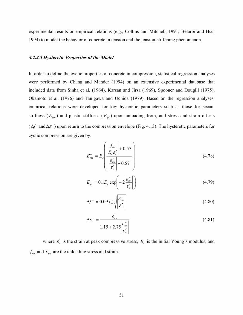
51
experimental results or empirical relations (e.g., Collins and Mitchell, 1991; Belarbi and Hsu,
1994) to model the behavior of concrete in tension and the tension-stiffening phenomenon.
4.2.2.3 Hysteretic Properties of the Model
In order to define the cyclic properties of concrete in compression, statistical regression analyses
were performed by Chang and Mander (1994) on an extensive experimental database that
included data from Sinha et al. (1964), Karsan and Jirsa (1969), Spooner and Dougill (1975),
Okamoto et al. (1976) and Tanigawa and Uchida (1979). Based on the regression analyses,
empirical relations were developed for key hysteretic parameters such as those for secant
stiffness ( secE ) and plastic stiffness ( plE ) upon unloading from, and stress and strain offsets
( fΔ and εΔ ) upon return to the compression envelope (Fig. 4.13). The hysteretic parameters for
cyclic compression are given by:
⎟⎟⎟⎟⎟
⎠
⎞
⎜⎜⎜⎜⎜
⎝
⎛
+′
+′
=−
−
−
57.0
57.0
sec
c
un
cc
un
c
Ef
EE
εε
ε (4.78)
⎟⎟⎠
⎞⎜⎜⎝
⎛′
−=−
−
c
uncpl EE
εε
2exp1.0 (4.79)
c
ununff
εε
′=Δ
−−− 09.0 (4.80)
c
un
un
εε
εε
′+
=Δ−
−−
75.215.1 (4.81)
where 'cε is the strain at peak compressive stress, cE is the initial Young’s modulus, and
unf and unε are the unloading stress and strain.

52
Strain, εc
Stre
ss, f
c
(εun,fnew)
(εre,fre)
Ec
Enew
Esec
Epl
Ec
(εpl,0)
(εun,fun)
Δε
Δf
Descending BranchAscending Branch( εc
' , f c' ) or (ε0+ εt , ft
)
r
1
1
1
1
1
Fig. 4.13 Hysteretic parameters of Chang and Mander (1994) model
Parameters such as the plastic (residual) strain upon unloading ( plε ), new stress ( newf )
and tangent modulus ( newE ) upon return to unloading strain from the envelope curve ( unε ), and
the strain ( reε ), stress ( ref ) and tangent modulus ( reE ) at the point of return to the envelope
curve are can be geometrically derived from these empirical relations (Fig. 4.13) as:
−
−−− −=
secEfun
unpl εε (4.82)
−−− Δ−= fff unnew (4.83)
−−
−−
−=
plun
newnew
fE
εε (4.84)
−−− Δ+= εεε unre (4.85)
⎟⎟⎠
⎞⎜⎜⎝
⎛′
=−
−−
c
rere ff
εε
(4.86)
⎟⎟⎠
⎞⎜⎜⎝
⎛′
=−
−−
c
rere EE
εε
(4.87)

53
For cyclic behavior in tension, Chang and Mander modified the empirical relations
defined in Equations 4.78–4.81, based on test results by Yankelevsky and Reinhardt (1987) as:
⎟⎟⎟⎟⎟
⎠
⎞
⎜⎜⎜⎜⎜
⎝
⎛
+−
+=
+
+
+
67.0
67.0
0sec
t
un
tc
un
c
Ef
EE
εεε
ε (4.88)
11.1
0 +−
=+
+
t
un
cpl
EE
εεε
(4.89)
++ =Δ unff 15.0 (4.90)
( )022.0 εεε −=Δ ++un (4.91)
where tε is the strain at peak tensile stress, cE is the initial Young’s modulus and 0ε is
the shifted origin of the tensile envelope curve. The derived parameters for tension are thus:
+
+++ −=
secEfun
unpl εε (4.92)
+++ Δ−= fff unnew (4.93)
++
++
−=
plun
newnew
fE
εε (4.94)
+++ Δ+= εεε unre (4.95)
⎟⎟⎠
⎞⎜⎜⎝
⎛ −=
+++
t
rere ff
εεε 0 (4.96)
⎟⎟⎠
⎞⎜⎜⎝
⎛ −=
+++
t
rere EE
εεε 0 (4.97)
A reversal from the compression envelope curve is done as shown in Figure 4.14, by
calculating the shifted origin ( )0ε of the tension envelope curve and evaluating the unloading
strain ( )+unε from the tension envelope curve. The variables that define this reversal curve are
calculated as follows:
Calculate the compression strain ductility as:

54
c
unux
εε
′=
−− (4.98)
Calculate the tension strain ductility:
t
unux
εεε 0−
=+
+ (4.99)
If −+ < uu xx , then:
−+ = uu xx (4.100)
00 =ε (4.101)
tuun x εε ++ =
( )+++ = ucun xff using Eq. 4.71 (4.102)
Calculate:
−+
+
+=Δ
pl
un
EEf
sec0
2ε (4.103)
Finally,
tupl x εεεε +− −Δ+= 00 (4.104)
0εεε += ++tuun x (4.105)
Accordingly, upon each unloading from the compression envelope, the origin of the
tension envelope is shifted based on the unloading strain from the compression envelope ( )−unε ,
and the unloading strain from the tension envelope ( )+unε is re-evaluated so that it corresponds to
a tension strain ductility equal to the compression strain ductility experienced just before
unloading from the compression envelope, or a previously experienced actual tension strain
ductility, whichever is greater.

55
(ε0
, 0)( εpl- ,0)
Strain, εc
Stre
ss, f
c
O
TensionNot to scale
Compression
Ec
1
1
11
( εun+
, f un+ )
( εpl+
,0)
( εun-
, f un- )
( εre+
, f re+ ) ( εun
+
, f new+ )
Epl-
Esec-
Esec+
Fig. 4.14 Unloading from compression envelope curve (Chang and Mander, 1994)
In terms of modeling generalized hysteretic behavior, the constitutive model uses smooth
“connecting” curves for unloading and reloading between the compression and tension envelope
curves, and smooth “transition” curves for partial unloading and reloading between the
connecting curves (Fig. 4.15). The connecting and transition curves are geometrically defined
such that they commence at the prescribed starting point (e.g., unε , unf in Fig. 4.13) with a
prescribed initial slope (e.g., cE ), and end up at a prescribed final (target) point (e.g., plε , 0 ) with
a prescribed final slope (e.g., plE ). Both connecting and transition curves and have slope
continuity with uniform sign of curvature (second strain derivative of the curve equation) in
between the starting and final points.

56
Strain, εc
Stre
ss, f
c
O
TensionNot to scale
Compression( ε c
' , f c' )
(ε0, 0)
(ε0+ εt, ft)
Fig. 4.15 Continuous hysteresis in compression and tension (Chang and Mander, 1994)
Chang and Mander (1994) proposed empirical expressions for determining the position of
the target points for the transition curves. As shown in Figure 4.16, which illustrates the
transition between two connecting curves before cracking, a reversal from the connecting curve
at point A ( )aa f,ε will target point B ( )bb f,ε through a transition curve, and an incomplete
loading on the same transition curve (i.e., unloading prior to the passing of point B) will target
the point A ( )aa f,ε again through a transition curve in the opposite direction. The relation
between points A and B is computed through the relation:
+−
−
−+
−
−−
=−−
plun
bun
plun
pla
εεεε
εεεε
(4.106)
After cracking, the tension envelope is zero, and the connecting curve upon unloading
(i.e., strain reversal) represents gap closure (Fig. 4.17). A reversal from the gap closure –
connecting curve at point A ( )aa f,ε targets the horizontal axis at a strain bε through a transition
curve. The target strain bε is calculated by the expression:
−−=secEfa
ab εε (4.107)

57
Strain, εc
Stre
ss, f
c
TensionNot to scale
Compression
( εpl- ,0)
( εun+
, f un+ )
( εpl+
,0)
( εun-
, f un- )
( εb
, f b)
( εa
, f a)
Connecting Curve
Connecting Curve
Transition Curve
Transition Curve
Fig. 4.16 Transition curves before cracking (Chang and Mander, 1994)
Strain, εc
Stre
ss, f
c
Tension
Compression
( εa
, f a)
( εb
,0)
Post-Cracking Connecting Curve(Gap Closure)
Transition Curves
Fig. 4.17 Transition curves after cracking (Chang and Mander, 1994)

58
Reversal from the transition curve will target the point A again (Fig. 4.17). The initial
slope of each transition curve (in Figs. 4.16–4.17) is equal to the concrete initial Young’s
modulus ( )cE , whereas the final slope is equal to the slope of the connecting curve at the target
(final) point of the transition curve.
The generalized equation used in the constitutive model to represent the connecting and
transition curves takes the form:
( )[ ]RIcIIcIc AEff εεεε −+−+= (4.108)
( ) RIcI
c
ct RAE
fE εε
ε−++=
∂∂
= 1 (4.109)
in which,
ISEC
SECF
EEEE
R−
−= (4.110)
RIF
ISEC EEA
εε −−
= (4.111)
with,
IF
IFSEC
ffE
εε −−
= (4.112)
where cf is the concrete stress, cε is the concrete strain, tE is the concrete tangent
modulus, If is the stress at initial point, Ff is the stress at final (target) point, Iε is the strain at
initial point, Fε is the stress at final point, IE is the tangent modulus at initial point, FE is the
tangent modulus at final point, SECE is the secant modulus between the initial and final points,
and R and A are equation parameters. The equations represent a stress-strain relation with
single sign of curvature and slope continuity between the initial and target points.
It has been observed in this study that the hysteretic rules of the Chang and Mander
model occasionally yield some minor numerical inconsistencies. For some strain histories, using
connecting and transition curves with no change in the sign of the curvature is geometrically
incompatible for commencing at a starting point with a prescribed initial slope and ending at a
target point with a prescribed ending slope. For example, the stress-strain history shown in
Figure 4.18 would require the connecting or transition curve that commences at the starting point
(e.g., +unε , +
newf ), with the initial slope (e.g., +newE ); to have changes in the sign of curvature in order

59
to reach the target point (e.g., +reε , +
ref ), with the ending slope ( +reE ). Similar conditions persist
upon unloading from the tension envelope. For such cases, where curves with uniform sign of
curvature are geometrically insufficient, a straight line with a secant slope was adopted here to
represent the connecting or transition curve between the starting and target points (Fig. 4.18).
Strain, εc
Stre
ss, f
c
Ec
( εun+
, f un+ )
Δf +
( εun+
, f new+ )
( εre+
, f re+)
Δε+
(double curvature required)
>Esecant Ec
(unlikely)
(ε0,0) ( εpl+
,0)
(ε0+εt, ft)Tension
Fig. 4.18 Numerical instabilities in hysteretic rules
Another inconsistency in the model is associated with the value of this secant slope. For
the same example strain history (Fig. 4.18), and for a range of values for unloading tensile strain
(roughly for tun εεε 5.00 +<+ ), using the stress and strain offsets ( +Δf and +Δε ) of Mander and
Chang can result in a value of the secant modulus which is larger than the initial Young’s
modulus ( cE ).This is physically unlikely and may also lead to convergence problems in the
nonlinear solution algorithm. Under such exceptional conditions, for simplicity, the stress and
strain offsets in tension ( +Δf and +Δε ) were eliminated from the model in this study. It is
believed that the numerical inconsistencies in the model are primarily associated with the
hysteretic parameters defined for cyclic tension (Eqs. 4.88–4.91). The accuracy of the model
parameters for cyclic tension was validated with relatively limited experimental data from
Yankelevsky and Reinhardt (1987). Chang and Mander remarked that better
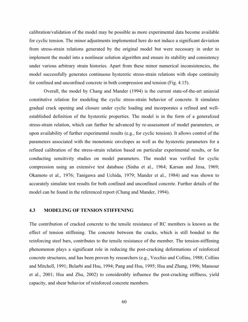
60
calibration/validation of the model may be possible as more experimental data become available
for cyclic tension. The minor adjustments implemented here do not induce a significant deviation
from stress-strain relations generated by the original model but were necessary in order to
implement the model into a nonlinear solution algorithm and ensure its stability and consistency
under various arbitrary strain histories. Apart from these minor numerical inconsistencies, the
model successfully generates continuous hysteretic stress-strain relations with slope continuity
for confined and unconfined concrete in both compression and tension (Fig. 4.15).
Overall, the model by Chang and Mander (1994) is the current state-of-the-art uniaxial
constitutive relation for modeling the cyclic stress-strain behavior of concrete. It simulates
gradual crack opening and closure under cyclic loading and incorporates a refined and well-
established definition of the hysteretic properties. The model is in the form of a generalized
stress-strain relation, which can further be advanced by re-assessment of model parameters, or
upon availability of further experimental results (e.g., for cyclic tension). It allows control of the
parameters associated with the monotonic envelopes as well as the hysteretic parameters for a
refined calibration of the stress-strain relation based on particular experimental results, or for
conducting sensitivity studies on model parameters. The model was verified for cyclic
compression using an extensive test database (Sinha et al., 1964; Karsan and Jirsa, 1969;
Okamoto et al., 1976; Tanigawa and Uchida, 1979; Mander et al., 1984) and was shown to
accurately simulate test results for both confined and unconfined concrete. Further details of the
model can be found in the referenced report (Chang and Mander, 1994).
4.3 MODELING OF TENSION STIFFENING
The contribution of cracked concrete to the tensile resistance of RC members is known as the
effect of tension stiffening. The concrete between the cracks, which is still bonded to the
reinforcing steel bars, contributes to the tensile resistance of the member. The tension-stiffening
phenomenon plays a significant role in reducing the post-cracking deformations of reinforced
concrete structures, and has been proven by researchers (e.g., Vecchio and Collins, 1988; Collins
and Mitchell, 1991; Belarbi and Hsu, 1994; Pang and Hsu, 1995; Hsu and Zhang, 1996; Mansour
et al., 2001; Hsu and Zhu, 2002) to considerably influence the post-cracking stiffness, yield
capacity, and shear behavior of reinforced concrete members.

61
Upon development of the original MVLEM by Vulcano et al. (1988), tension stiffening
was modeled using an axial-element-in-series model (AESM) (Fig. 4.19) to describe the
response of the uniaxial sub-elements of the model. The two elements in series represented the
segment along the uniaxial elements in which the bond remained active (element 1) and the
segment for which the bond stresses were negligible (element 2). The concrete within element 1
was considered to be uncracked and modeled with a linear elastic behavior. The cracked concrete
within element 2 was considered to have no contribution (zero stresses) to the axial stiffness of
the AESM under increasing tensile strains. A dimensionless parameter λ was introduced to
define the relative length of the two elements (representing cracked and uncracked concrete) to
account for tension stiffening. Under monotonic tensile loading, the tension-stiffening effect was
incorporated by manipulating the value of the dimensionless parameter λ such that the tensile
stiffness of the uniaxial model in Figure 4.19 would be equal to the actual (experimentally
observed) tensile stiffness of a tension stiffened uniaxial element evaluated on the basis of an
empirical law suggested by proposed by Rizkalla and Hwang (1984).
(1-λ)h
λh
h
F , Δ
Steel
Steel
Concrete (uncracked)
Concrete(cracked)
Element 1
Element 2
Fig. 4.19 Axial-element-in-series model
The law suggested by Rizkalla and Hwang (1984) relates the ratio of the steel strain
within cracks to the average strain of a reinforced concrete member under monotonic axial
tensile loading. Under cyclic loading, it was assumed that the value of λ was kept constant
during unloading from the tensile stress state, equal to the value corresponding to the maximum

62
tensile strain previously attained; if this maximum strain was exceeded during a tensile
reloading, the value of λ was updated as for the case of monotonic tensile loading.
In this study, instead of the AESM, a two-parallel-component model (Colotti, 1993) (Fig.
4.20) is adopted for the uniaxial elements of the present wall model, and concrete and steel
within each uniaxial element are subjected to the same average (smeared) strains. The tension-
stiffening effects are directly incorporated into the constitutive stress-strain relations
implemented for concrete and steel, as described in the following paragraphs.
Steel Concreteh
F , Δ
Fig. 4.20 Two-parallel-component-model
As investigated in detail by Belarbi and Hsu (1994), modeling of the tension-stiffening
phenomenon must consider two effects simultaneously. First, an average (smeared) tensile
stress-strain curve must be considered for cracked concrete; and second, the stress-strain curve of
bare mild steel bars must be replaced by an average (smeared) stress-strain curve for steel bars
stiffened by concrete between cracks. Accordingly, based on extensive tests of reinforced
concrete panels subjected to normal stresses, Belarbi and Hsu (1994) developed two constitutive
models: one for the average tensile stress-strain relation of concrete and one for the average
tensile stress-strain relation of steel reinforcing bars stiffened by concrete. The tension-stiffening
models proposed by Belarbi and Hsu have also been used and validated experimentally in more
recent studies to model the shear behavior of RC membrane elements (e.g., Pang and Hsu, 1995;
Hsu and Zhang, 1996; Mansour, Lee, and Hsu, 2001; Hsu and Zhu, 2002).
The average stress-strain relation proposed by Belarbi and Hsu for concrete in tension
takes the form (Fig. 4.21):

63
If crc εε ≤ then ccc E εσ = (4.113)
If crc εε > then 4.0
⎟⎟⎠
⎞⎜⎜⎝
⎛=
c
crcrc f
εεσ (4.114)
where:
)(3875 MPafE cc ′= (4.115)
)(31.0 MPaff ccr ′= (4.116)
00008.0=crε (4.117)
In the equation above, cε is the average concrete tensile strain, cσ is the average
concrete tensile stress, cE is the initial Young’s modulus of the average stress-strain relation, crf
is concrete the tensile cracking stress, and crε is the concrete strain at cracking.
0 0.002 0.004 0.006 0.008 0.01
Strain, εc
0
0.5
1
1.5
2
2.5
Stre
ss, σ
c (M
pa)
fcr
εcr
Fig. 4.21 Average stress-strain relation by Belarbi and Hsu for concrete in tension
The relation consists of an ascending straight line before cracking and a descending curve
to the power of 0.4 after cracking (Fig. 4.21). The expressions for crf , crε , cE , and the power
constant 0.4 in Equation (4.117) are obtained from the average and best fit of experimental
crc εε ≤ ccc E εσ =
crc εε > 4.0
⎟⎟⎠
⎞⎜⎜⎝
⎛=
c
crcrc f
εεσ
)(3875 MPafE cc ′=
)(31.0 MPaff ccr ′=
00008.0=crε

64
results from testing 17 RC panels with concrete cylinder compressive strengths ranging between
36.9 MPa and 47.7 MPa.
Belarbi and Hsu (1994) also identified how the average stress-strain relation of
reinforcing steel bars surrounded by concrete is different than the stress-strain relation of bare
steel bars (Fig. 4.22).
0 0.005 0.01 0.015 0.02 0.025 0.03 0.035 0.04
Strain
0
100
200
300
400
500
600
Stre
ss (M
Pa)
Bare BarBar Surrounded by Concrete
Fig. 4.22 Effect of tension stiffening on reinforcing bars
The most important difference was found to be the lowering of the yield stress, yσ , as
yielding of a reinforced concrete element occurs when the steel stress at the cracked section
reaches the yield strength of the bare bar. At the same time, the average steel stress smeared
along the length of the element reaches a level lower than that of the yield stress of the bare bar.
Based on experimental data from the RC panels, the reduction of the yield stress of bars
embedded in concrete were found to be empirically dependent on the cross-sectional area ratio of
the longitudinal steel in the panel ( )ρ and the ratio of concrete cracking stress ( )crf to the steel
yield stress ( )yσ . The strain-hardening slope (plastic modulus) of the steel bars embedded in
concrete was also observed to differ from the plastic modulus of bare bars with the variation also
dependent on the above parameters.

65
Based on evaluation and characterization of experimental data from the RC panels,
Belarbi and Hsu (1994) proposed a simple bilinear constitutive model for steel bars embedded in
concrete (Fig. 4.23). The stress-strain relation is represented by two straight lines, the first
straight line with a slope sE (steel modulus of elasticity) covering the elastic range of strains,
and the second straight line with a slope *pE representing the plastic range.
The stress at the intersection of the two lines ( )*nσ and the plastic slope ( )*
pE are given by
the following expressions:
( ) yn B σσ 293.0* −= (4.118)
sp EBE )25.002.0(* += (4.119)
where the parameter B is defined as:
5.1
1⎟⎟⎠
⎞⎜⎜⎝
⎛=
y
crfB
σρ (4.120)
In the equations above, yσ and sE are the yield stress and modulus of elasticity of the
bare steel bars, ( )ρ is the cross-sectional area ratio of the longitudinal steel bars in the RC
element (limited to a minimum of 0.25% in Mansour, Lee and Hsu, 2001), and ( )crf is the
concrete cracking stress, obtained according to the relation in Equation 4.116. Equation 4.119
was derived assuming that the plastic modulus of “bare” steel bars ( )pE is approximately equal
to 2.5% of the modulus of elasticity ( )sp EE 025.0= . For a more general case, Equation 4.119
can be expanded as:
sp EBbE )25.08.0(* += (4.121)
where b is the strain-hardening ratio ( )sp EE defined for the bare steel bars.
Accordingly, the bilinear model of Belarbi and Hsu (1994) for modeling the average
(smeared) stress-strain behavior of steel reinforcing bars embedded in concrete takes the form
(Fig. 4.23):
If ns εε ≤ , sss E εσ = (4.122)
If ns εε > , ( ) ( ) ( )nssys EBbB εεσσ −++−= 25.08.0293.0 (4.123)

66
0 0.005 0.01 0.015 0.02
Strain, εs
0
200
400
600
Stre
ss, σ
s (M
pa)
σn*
εn
Fig. 4.23 Average stress-strain relation by Belarbi and Hsu (1994) for reinforcing bars embedded in concrete
where sσ is the average stress, sε is the average strain, nε is the average strain defined
at the intersection of the two lines:
( )
s
y
s
nn E
BE
σσε293.0* −
== (4.124)
and sE , yσ , and b are the modulus of elasticity, yield stress, and strain-hardening ratio
experimentally measured for bare steel bars.
The constitutive relations implemented in the present wall model for concrete and steel
can be controlled and calibrated to follow accurately the relations developed by Belarbi and Hsu
(1994) (or similar average stress-strain relations) to model tension stiffening for monotonic
loading. For example, Figure 4.24 shows a comparison of a representative tension envelope
curve (or monotonic tensile stress-strain curve) generated by the Chang and Mander model
(1994) with the average stress-strain relation proposed by Belarbi and Hsu (1994) for concrete.
ns εε ≤ sss E εσ =
ns εε > ( ) ( ) ( )nssys EBbB εεσσ −++−= 25.08.0293.0
( )s
yn E
B σε
293.0 −=
5.11
⎟⎟⎠
⎞⎜⎜⎝
⎛=
y
crfB
σρ

67
0 0.0005 0.001 0.0015 0.002 0.0025
Strain
0
0.5
1
1.5
2
2.5
Stre
ss (M
Pa)
Chang and Mander (1994)Belarbi and Hsu (1994)
0 0.005 0.01 0.015 0.02 0.025 0.03
0
0.5
1
1.5
2
2.5(εt ,ft )
r
Fig. 4.24 Stress-strain relations for concrete in tension
The shape of the tension envelope curve in Chang and Mander’s model is conveniently
controlled through the shape parameter r (in addition to the initial Young’s modulus cE , the
peak tensile stress tf , and the strain at peak tensile stress tε ) (Figs. 4.11 and 4.13). The primary
difference in the two tension envelopes is that the envelope generated using the Chang and
Mander model also accounts for the nonlinearity of the stress-strain relation prior to cracking (as
observed experimentally by Yankelevsky and Reinhardt, 1987). Similarly, the tensile elastic and
yield asymptotes in the steel stress-strain model by Menegotto and Pinto (1973) (which
constitute the monotonic tensile stress-strain relation) can be calibrated through the parameters
yσ (yield stress) and b (strain-hardening ratio) to precisely follow the bilinear stress-strain
relation of Belarbi and Hsu for steel bars embedded in concrete (Fig. 4.25).
To model the tension-stiffening effects under cyclic loading, the calibrated monotonic
stress-strain relations will be used in this study as the tension envelope curve for concrete and the
tensile elastic and yield asymptotes for steel, together with the unloading and reloading rules of
the hysteretic constitutive models described in the previous sections. On the whole, the approach
adopted here to model tension stiffening is a more refined and up-to-date methodology compared
to the one that involves the use of the axial-element-in-series model (AESM) as implemented by

68
0 0.005 0.01 0.015 0.02 0.025 0.03 0.035
Strain
-600
-400
-200
0
200
400
600
800
Stre
ss (M
Pa)
Menegotto and Pinto (1973)Belarbi and Hsu (1994)
Fig. 4.25 Stress-strain relations for reinforcing bars
Vulcano et al. (1988) in the original MVLEM. The tension-stiffening phenomenon is
incorporated at the material level, considering the effects on both steel and concrete, based on a
more robust and manageable theory as well as extensive experimental studies.
4.4 SUMMARY
Since the MVLEM adopted in this study relates the analytical response directly to uniaxial
material behavior, extensive consideration was given to the selection and refinement of the
robust and state-of-the-art constitutive relations implemented in the analytical model. For an
accurate and reliable prediction of wall flexural response, it was necessary that the relations
selected had been validated with extensive experimental data.
The reinforcing steel stress-strain behavior implemented in the wall model is the widely
used nonlinear hysteretic model of Menegotto and Pinto (1973), as extended by Filippou et al.
(1983) to include isotropic strain-hardening effects. This model was shown to be capable of
reproducing experimental results with accuracy; the model results agree very well with
experimental results from cyclic tests on reinforcing bars (e.g., Menegotto and Pinto, 1973;
Filippou et al., 1983; Elmorsi et al., 1998).

69
Two different constitutive models for concrete (Yassin, 1994; Chang and Mander, 1994)
were adopted in the present wall model. Both models address important issues such as the
hysteretic behavior in continuous cyclic compression and tension, the progressive degradation of
stiffness of the unloading and reloading curves for increasing values of strain, and the effects of
confinement and tension stiffening. However, the Chang and Mander model (1994), being the
current state-of-the-art uniaxial constitutive relation for modeling the cyclic stress-strain
behavior of concrete, is clearly superior to the hysteretic model by Yassin (1994). The Chang
and Mander model is a generalized constitutive model that allows control of the parameters
associated with the monotonic envelopes, as well as the hysteretic parameters, for a refined
calibration of the stress-strain relation based on particular experimental results. For example,
Figure 4.26 compares the results of the Chang and Mander model and the model by Yassin, with
results of axial compressive stress-strain tests performed on standard cylinder specimens of
concrete used in the construction of a reinforced concrete structural wall specimen (Thomsen and
Wallace, 1995). By calibration of its parameters (parameters associated with the initial tangent
modulus, the peak stress, the strain at peak stress and the shape of the stress-strain curve), the
model by Chang and Mander can simulate the test results accurately; whereas the model by
Yassin (with the only parameters for calibration being the peak stress and the strain at peak
stress) fails to provide an accurate representation.
0 0.0005 0.001 0.0015 0.002 0.0025
Strain
0
10
20
30
40
50
Stre
ss (M
Pa)
Test Result (Thomsen and Wallace, 1995)Test Result (Thomsen and Wallace, 1995)Model by Chang and Mander (1994)Model by Yassin (1994)
Fig. 4.26 Compression envelopes for concrete — model vs. test results

70
Similarly, Figure 4.27 shows a comparison of the results of the Chang and Mander model
and the model by Yassin, with the relation developed by Belarbi and Hsu (1994) based on
experimental data, for the average tensile stress-strain behavior of concrete experiencing tension
stiffening. Again, the model by Yassin fails to represent the observed behavior accurately.
Furthermore, the Chang and Mander model successfully simulates the gradual closure of cracks
(Figs. 4.15, 4.17) under cyclic loading due to progressive contact stresses within the cracks. On
the other hand, the model by Yassin assumes sudden crack closure (Fig. 4.8), which may
significantly impair the accuracy in predicting the pinching properties of the RC wall modeled.
Due to these limitations, the model by Yassin was very seldom used in this study. It was
implemented in the wall model as a simple and widely used (e.g., OpenSees) alternative, and was
included in this chapter to signify the refinements of the model by Chang and Mander.
Finally, the modeling of the tension-stiffening phenomenon, as described in the previous
section, was performed at the material level, with effects on both concrete and steel considered,
based on a comprehensive theory and extensive experimental validation (Belarbi and Hsu, 1994).
0 0.0005 0.001 0.0015 0.002 0.0025
Strain
0
0.5
1
1.5
2
2.5
Stre
ss (M
Pa)
Chang and Mander (1994)Yassin (1994)Belarbi and Hsu (1994)
Fig. 4.27 Tension envelopes for concrete — model comparisons

71
The constitutive material models described in this chapter, and the formulation of the
MVLEM elements described in Chapter 3, were implemented in Matlab (MathWorks, 2001),
together with a direct stiffness assembly procedure to assemble the MVLEM elements into a
complete wall model and an incremental-iterative numerical scheme to perform nonlinear quasi-
static (monotonic or cyclic) analyses of the model. Details of the nonlinear analysis solution
strategy adopted in this study are described in the following chapter.

5 Nonlinear Analysis Strategy
The macro-wall-model elements formulated in Chapter 3 and the material constitutive relations
described in Chapter 4 were implemented in Matlab (MathWorks, 2001) together with a direct
stiffness assembly procedure to assemble the MVLEM elements into a complete wall model
(Fig. 5.1) and an incremental-iterative solution strategy to perform nonlinear quasi-static
(monotonic or cyclic) analysis of the wall model. The nonlinear analysis solution strategy
adapted is described in this chapter.
RC WALL WALL MODEL
1
2
3
4
1011
12
1314
15
k1 k2 k n kH. . . . .
1
2 3
45
6
k1 k2 k n kH . . . . .
Fig. 5.1 Sample model assembly with degrees of freedom
Various incremental-iterative numerical schemes can be implemented for the nonlinear
analysis of the wall model depending on the type of loading. For example, the conventional
force-controlled Newton-Raphson solution scheme can be adopted for nonlinear dynamic
analysis of the wall model. In this study in order to conduct a nonlinear quasi-static analysis of
the wall model, a displacement-controlled iterative solution strategy, based on a specified

74
incrementation of a selected displacement component (at a selected degree of freedom), was
adapted. In this strategy, iterations are performed on both displacement and load components to
obtain static equilibrium within a specified tolerance, while keeping constant the value of the
selected displacement component. This solution strategy was implemented in order to better
correlate the model response with drift-controlled cyclic test results on RC wall specimens which
are typically subjected to prescribed lateral displacement histories at the top of the wall (e.g.,
Thomsen and Wallace, 1995). Numerical solution strategies to conduct nonlinear analyses using
the model are described in the following sections.
5.1 NONLINEAR QUASI-STATIC PROBLEM
Quasi-static response is generated when the externally applied cyclic loads or displacements are
applied with a sufficiently slow loading rate that they do not induce dynamic effects. A nonlinear
analysis strategy that is capable of reproducing the entire nonlinear quasi-static response of the
multi-degree-of-freedom model, including load and displacement limits points within the static
load path of the model, is desired.
The nonlinear equilibrium equation associated with the quasi-static response can be
expressed as:
( ){ } { }extFF =δint (5.1)
where ( ){ }δintF is the internal resisting force vector, being a nonlinear functional of
system (nodal-degree-of-freedom) displacements, and { }extF is the external force vector,
representing the externally applied forces at the nodal degrees of freedom. It should be noted that
in the case of a linear elastic system, the static problem would reduce to the linear equation:
[ ]{ } { }extFK =δ (5.2)
where [ ]K denotes the stiffness matrix and { }δ is the vector of nodal displacements.
Equation (5.1) is a nonlinear algebraic equation in { }δ due to the nonlinear relation between the
resisting force vector { }intF and the vector of nodal displacements{ }δ .

75
5.2 INCREMENTAL ITERATIVE APPROACH — NEWTON-RAPHSON SCHEME
An iterative-incremental nonlinear analysis strategy is required to solve the nonlinear algebraic
equation for the quasi-static problem. The nonlinear equation can be linearized by the
conventional Newton-Raphson method, which forms a basis for various iterative strategies, and
solved for the vector of nodal displacements { }δ , by iterating within a load step until
convergence is achieved. Figure 5.2 illustrates a schematic of the Newton-Raphson solution
algorithm, with the incremental equation of equilibrium expressed as:
( ){ } { }extFF Δ=ΔΔ δint (5.3)
where ( ){ }δΔΔ intF is the incremental restoring force vector being a nonlinear functional
of the incremental nodal-displacement vector ( )δΔ , and { }extFΔ is the incremental external load
vector.
Equation (5.3) is linearized within an arbitrary load step i about { } { }iδδ = , yielding the
equation for the first iteration of the load step:
[ ] { } { }iextii FK Δ=Δ 11 δ (5.4)
where [ ]1iK denotes the tangent stiffness matrix of the system at the beginning of the load
step obtained by differentiating the nonlinear internal resisting force functional:
[ ] ( )( )
id
FdK i
δδδ =
= int1 (5.5)
The linearized incremental equilibrium equation for the j’th iteration of the Newton-
Raphson scheme within the load step i can be written as:
[ ] { } { } ji
ji
ji RK Δ=Δδ (5.6)
where
{ } { } { } 1int
1 −− Δ−Δ=Δ ji
ji
ji FRR (5.7)
The term { } jiRΔ represents the vector of residual forces (Fig. 5.2) and the term { } 1
int−Δ j
iF
is the increment of internal resisting forces for the iteration being equal to the difference between
the two internal resisting force vectors: { } { } 2int
1int
−− − ji
ji FF (Fig. 5.3).

76
{ } { }1iiext RF Δ=Δ
{ }iδ{ }iδΔ
[ ]1iK
{ }extF
{ }δ
{ }2iRΔ
{ }1int iFΔ
{ }2int iFΔ
{ }3iRΔ
{ }iextF
{ } 1+iextF
[ ]2iK
{ } 1+iδ
{ }1iδΔ { }2
iδΔ
Fig. 5.2 Newton-Raphson iteration scheme
{ }iδ { } 1+iδ
{ }intF
{ }δ
{ } 1int +iF
{ }11+iδ { }2
1+iδ
{ }1iδΔ { }2
iδΔ
{ }iFint
{ }11int +iF
{ }21int +iF
{ }1int iFΔ
{ }2int iFΔ
Fig. 5.3 Nodal-displacement and internal resisting-force increments
Solving for { } jiδΔ within successive iterations, convergence is achieved by minimizing
the vector of residual forces to a specified value of tolerance. The resulting incremental nodal-
displacement vector for the ith load step can be computed as the sum:

77
{ } { } { } { }liiii δδδδ Δ++Δ+Δ=Δ ..........21 (5.8)
where l is the number of iterations performed in order to achieve convergence. The
strategy follows the same scheme in subsequent load steps.
Although the well-known Newton-Raphson strategy successfully linearizes the
equilibrium equation to obtain an iterative solution, it is incapable of passing load limit points
(Fig. 5.4) within the quasi-static load-displacement path of the system because the load level is
held constant while iterations are conducted to achieve convergence. It is included here to
provide a solid basis for a more complex iterative strategy described in following subsection.
Load Limit Point
Load Limit Point
Displacement
Load
Fig. 5.4 Load limit points within sample quasi-static load-displacement path
For incremental nonlinear analysis approaches, passing load limit points is extremely
difficult due to the near singular nature of the tangent stiffness matrix in the neighborhood of a
load limit point. Iterations should be performed on externally applied loads as well as nodal
displacements by introducing constraint equations within the solution strategy to proceed beyond
a load limit point. Several different techniques have been proposed for this purpose, the most
well known being “iteration at constant arc-length” introduced by Wempner (1971) and updated
by Ricks (1979). The iterative solution technique that has been used in this study is an adaptation
of the arc-length method, with a displacement-controlled iterative strategy, based on
incrementation of selected displacement components of the model (see also Clarke and Hancock,
1990). Details of the iterative strategy are presented in following sections. The strategy was
selected in order to correlate the model responses with results for drift-controlled cyclic test

78
results on RC wall specimens (described in Chapter 7). The selected displacement component to
be incremented throughout the nonlinear analysis is thus along the horizontal degree of freedom
at the top of the wall model.
5.3 APPLIED NONLINEAR ANALYSIS SOLUTION STRATEGY
An incremental-iterative displacement-controlled solution technique was implemented for
nonlinear analysis using a MVLEM for RC walls. The hysteretic constitutive material relations
were used to determine global nonlinear hysteretic structural response based on satisfying both
equilibrium conditions and force-deformation relations at each load step. The solution method
described is based on a modified Newton-Raphson approach, that is, the tangent stiffness matrix
is computed at the beginning of each load step and held constant for each load step. An iterative
strategy, based on constant displacements with incrementation of selected displacement
components was used for the purpose of passing load limit points and to allow comparison with
experimental results.
The incremental-iterative solution strategy described here is ideally suited for obtaining
the complete static load–deflection response of a structural model. In the incremental-iterative
method, each load step consists of the application of an increment of external load with
subsequent iterations required to satisfy the total equilibrium equations within a specified
tolerance. In this text, the notation adopted is to use the subscript i to denote load step number i,
and the superscript j to denote the iteration cycle j (within load step i). Iteration cycles begin at
1=j , which is defined to correspond to an increment of external load. The equilibrium iterations
commence at 2=j . The scalar λ denotes a load parameter to be used in combination with a
reference external load vector (assuming external loading to be proportional), and { }δ is the
vector of nodal displacements at the model degrees of freedom. There are two distinct strategies
required for the successful completion of a single load step in an incremental-iterative scheme:
1. Selection of a suitable external load increment 1iλΔ for the first iteration cycle. The
selected increment is referred to as the “initial load increment,” and the particular
strategy used to determine it is referred to as the “load incrementation strategy.”
2. Selection of an appropriate “iterative strategy” for use in subsequent iterative cycles
( 2≥j ) where the aim is to restore equilibrium as rapidly as possible. If iterations are

79
performed on the load parameter jiλΔ as well as on the nodal displacements { }j
iδ ,
then an additional constraint equation involving jiλΔ is required. It is the form of this
constraint equation that distinguishes the various iteration strategies.
A description of the incremental-iterative technique for a single load step i is described in
the following subsections. It is assumed that perfect convergence has been achieved at the
conclusion of load step ( 1−i ) so that the solution { }( )1,1 −− ii δλ is known to satisfy total
equilibrium (Fig. 5.5).
5.3.1 First Iteration Cycle, j = 1
The new load step starts with the computation of the tangent stiffness matrix [ ]iIK based on the
known displacements (strains) and loads (stresses) at the conclusion of the previous load step.
The “tangent” displacements { }iIδ for this load step are then computed as the solution of:
[ ] { } { }iIiIiI FK =δ (5.9)
in which { }iIF is the reference external load vector, typically as specified in the input
data for the problem. The magnitude of the tangent displacements is arbitrary, only their
direction is important. Next, the value of the initial load increment 1iλΔ is determined according
to a particular load incrementation strategy, referred to as the “incrementation of a selected
displacement component” in this study. The incremental displacements are then evaluated by
scaling the tangent displacements:
{ } { }iIii δλδ 11 Δ=Δ (5.10)
The total displacements and load level are updated from those existing at the conclusion
of the previous load step (Fig. 5.5) as:
{ } { } { }11
1iii δδδ Δ+= − (5.11)
11
1iii λλλ Δ+= − (5.12)
At this stage the solution does not satisfy total equilibrium within the specified tolerance,
so additional iterative cycles are required to restore equilibrium.

80
5.3.2 Equilibrium Iteration Cycles, j ≥ 2
The well-known Newton-Raphson or modified Newton-Raphson iterative strategies are
incapable of passing limit points because the load level is held constant while iterating to obtain
convergence; therefore, the load parameter jiλΔ must be allowed to vary if limit points are to be
overcome. With a varying load parameter, a general solution technique evolves if it is assumed
that for any iteration 2≥j within load step i, the change in the incremental displacements can be
expressed as:
[ ] { } { } { } 1−−Δ=Δ jiiI
ji
jiiI FK ψλδ (5.13)
where,
{ } { } { } 11int
1 −−− −= jiext
ji
ji FFψ (5.14)
Equation (5.14) represents the net internal out-of-balance (or “residual”) force acting on
the structure at the conclusion of the previous iteration. The vector { } 1int
−jiF represents the
internal nodal forces obtained at equilibrium from element contributions (forces in the uniaxial
elements and horizontal springs in the present model). For proportional loading, the external
forces { } 1−jiextF at the conclusion of the previous iteration may be expressed as:
{ } { }iIji
jiext FF 11 −− = λ (5.15)
The right-hand side of the equation (5.13) is linear in jiλΔ ; thus the final solution can be
written as the linear combination of two vectors:
{ } { } { }jiRiI
ji
ji δδλδ Δ+Δ=Δ (5.16)
in which { }iIδ are the tangent displacements, already computed for 1=j , and { }jiRδΔ are
the “residual” displacements (Fig. 5.6) obtained from Equation (5.17):
[ ] { } { } 1−−=Δ ji
jiRiIK ψδ (5.17)
The variation of the load parameter jiλΔ is obtained by solving an appropriate constraint
equation, as described in the following subsection. The incremental change to the nodal
displacements for this iteration is computed using Equation (5.16), and the total displacements
and load level are updated from the previous iteration (Fig. 5.5) as:
{ } { } { }ji
ji
ji δδδ Δ+= −1 (5.18)

81
ji
ji
ji λλλ Δ+= −1 (5.19)
Displacement, δ
Load
Par
amet
er,
λ
Converged state (i-1)
New convergedstate i
Iterative path
(Δλ) i1
- (Δλ) i2
(Δδ) i1 (Δδ) i
2
δ i-1 δ i1 δ i
2 δ i...
λ i-1
λ i1
λ i2
λ i
...
Fig. 5.5 Representation of adapted nonlinear analysis solution scheme for single-degree-of-freedom system
Iteration cycles are continued until a convergence criterion based on either the structure
forces or displacements is satisfied. If convergence is not achieved within a specified number of
cycles, or if divergence of the solution is detected, a re-solution strategy may be adopted. The
convergence criterion and the re-solution scheme used in this study are described in a subsequent
section.

82
Displacement, δ
Load
Par
amet
er,
λ
New convergedstate i
- (Δλ) i2
δ i1 δ i
2 δ i...
λ i1
λ i2
λ i
...
(ΔδR) i2
- (Δλ) i2(δI)i
Fig. 5.6 Iterative strategy and residual displacements
5.3.3 Incrementation Strategy: Incrementation of Selected Displacement Component
The analysis results are to be calibrated and compared with lateral drift-controlled cyclic tests
performed on RC wall specimens as described in Chapter 7. In order to simulate the test
conditions, an incrementation strategy based on a selected displacement component is adopted in
the nonlinear analysis strategy. The initial load increment of each load step is chosen to limit a
specified “key” displacement nδ (being the lateral top displacement of the wall in this study) in
the structure. If it is assumed that perfect convergence is achieved at the conclusion of the
previous load step, the displacement increment ( )inδΔ can be expressed as:
( ) { } { }iIT
niin b δλδ 1Δ=Δ (5.20)
in which { }nb is a vector containing unity in the nth row and zero elsewhere. Hence,
( )
{ } { }iIT
n
ini b δ
δλ
Δ=Δ 1 (5.21)

83
5.3.4 Iterative Strategy: Iteration at Constant Displacement
The constant displacement iteration strategy described here is an example of a more general
technique presented by Powell and Simons (1981). It was adopted in this study in order to
perform a displacement-controlled analysis that successfully proceeds beyond load limit points,
defined as the points of load reduction within the static load path of a structure, where softening
behavior is initiated (Fig. 5.4).
In the first iteration ( 1=j ), the key displacement component in the structure ( nδ in this
case) is incremented by a prescribed amount as described in the preceding subsection. This
displacement component is held constant during subsequent iterations ( 2≥j ). Denoting the key
displacement component as nδ , the nth component in the vector of nodal degrees of freedom, the
increment in nδ can be expressed as:
{ } { }jiR
Tnn b δδ Δ=Δ (5.22)
in which { }nb is a vector of zero entries except for unity in the nth row. From equation
(5.16),
{ } { } { } { }jiR
TniI
Tn
jin bb δδλδ Δ+Δ=Δ (5.23)
If the value of nδ is to remain unchanged during the equilibrium equations (constant
displacement) then nδΔ =0, giving the iterative change in the load parameter:
{ } { }{ } { }iI
Tn
jiR
Tnj
i bb
δδ
λΔ−
=Δ (5.24)
5.3.5 Convergence Criteria and Re-Solution Strategy
Within the analysis, iteration cycles are continued until a convergence criterion based on
structure displacements is satisfied at the end of each load step. If convergence is not achieved
within a specified number of cycles, a re-solution strategy for that load step is selected in this
study.
A convergence criterion based on the incremental displacements is used. The stringent
maximum norm is adopted in the present study to test for convergence, that is:

84
Maximum norm: k
k
k δδε Δ
=∞
max (5.25)
where kδΔ is the change in the displacement component k during the current iteration
cycle and kδ is the value of that displacement component updated at the end of the previous
iteration. Convergence is attained when:
cζε <∞
(5.26)
where the tolerance cζ is typically in the range of 10-2 to 10-5 depending on the desired
accuracy.
In the solution technique described above, a re-solution strategy was incorporated. A re-
solution is necessary if convergence is not attained at each load step within the maximum
specified number of iterative cycles or if the solution appears to be diverging. An increase of
stiffness within a single load step is the most frequently encountered reason for nonconvergence
for the MVLEM. The re-solution is facilitated by recovering the previous converged load step at
displacement level{ } 1−iδ , and starting the current load step over using the initial stiffness matrix
of the first load step (undeformed configuration). If convergence is still not attained within the
number of specified iterations, the value of the prescribed displacement increment nδΔ is
changed (usually decreased), and the current step is repeated until an increment that satisfies
convergence and complies with the applied displacement history, is found.
5.4 SUMMARY
The incremental-iterative solution strategy implemented in this study is ideal for obtaining the
complete quasi-static load-deflection response of the analytical wall model. Iterations are
performed on both displacement and load components to obtain static equilibrium within a
specified tolerance, while keeping the value of a selected displacement component (e.g., lateral
displacement at the top of the wall) constant. Calibration of the analytical model and comparison
of model results with results of lateral drift-controlled cyclic tests performed on RC wall
specimens is presented in Chapter 7. The following chapter (Chapter 6) describes attributes of
the analytical model response and sensitivity of model results to model and material parameters.

6 Flexural Modeling — Analytical Model Results and Parametric Sensitivity Studies
The macro wall model formulated in Chapter 3 and the material constitutive relations described
in Chapter 4 were implemented in Matlab (MathWorks, 2001) together with the incremental-
iterative solution strategy described in Chapter 5 to perform nonlinear quasi-static analyses of the
analytical wall model. Attributes of the analytical model response and sensitivity of the model
results to both model and material parameters are presented in this chapter.
6.1 REVIEW OF ANALYTICAL MODEL
The multiple-vertical-line-element model (MVLEM), as implemented in this study, is an
effective and robust modeling and analysis tool for predicting the inelastic response of RC walls
and wall systems. The model incorporates important material characteristics and behavioral
response features such as neutral axis migration, tension-stiffening, progressive gap closure,
concrete confinement, nonlinear shear behavior, and the effect of fluctuating axial force on
strength and stiffness. A detailed description of the model and implemented constitutive relations
were presented in Chapters 3 and 4, respectively. A brief review of the model attributes and
material constitutive features is provided in the following paragraphs.
A structural wall is modeled as a stack of m MVLEM elements, which are placed one
upon the other (Fig. 6.1). The flexural response is simulated by a series of uniaxial elements (or
macro-fibers) connected to infinitely rigid beams at the top and bottom (e.g., floor) levels. The
primary simplification of the model involves applying the plane-sections-remain-plane
assumption in calculating the strain level in each uniaxial element according to values of
displacement or rotation at the degrees of freedom of each wall element. The stiffness properties
and force-displacement relations of the uniaxial elements are defined according to detailed
constitutive stress-strain relations implemented in the model for concrete and steel and the

86
tributary area assigned to each uniaxial element (Fig. 6.2). The strains in concrete and steel are
typically assumed to be equal (perfect bond) within each uniaxial element. The relative rotation
between the top and bottom faces of the wall element occurs around the point placed on the
central axis of the element at height ch. A suitable value of the parameter c is based on the
expected curvature distribution along the element height h. A horizontal spring placed at the
height ch, possibly with a nonlinear hysteretic force-deformation relation, simulates the shear
response of the wall element. However, this study focuses on modeling of the flexural response,
thus a linear elastic force-deformation behavior was adopted for the horizontal “shear” spring.
For the present model, flexural and shear modes of deformation of the wall member are
uncoupled (i.e., flexural deformations do not affect shear strength or deformation), and the
horizontal shear displacement at the top of the element does not depend on c.
h
(1-c)h
ch
1 2
3
4 5
6 Rigid Beam
Rigid Beam
k 1 k 2 knk H . . . . . . .
m
RC WALL WALL MODEL
1
2
. . . . .
(a) MVLEM element (b) Model of a wall
Fig. 6.1 Multiple-vertical-line-element model
1k 32k k4k 5k 6k 87k k
Fig. 6.2 Tributary area assignment
The reinforcing steel stress-strain behavior implemented in the wall model is the well-
known nonlinear relation of Menegotto and Pinto (1973) (Fig. 6.3), as extended by Filippou et al.
(1983) to include isotropic strain-hardening effects.

87
-0.01 -0.005 0 0.005 0.01 0.015 0.02
Strain, ε
-600
-400
-200
0
200
400
600
Stre
ss, σ
(M
Pa)
εy
E0
E1= bE0(εr
1,σr1)
(εr2,σr
2)(ε0
1,σ01)
(ε02,σ0
2) σy
σ*= b ε*+ (1-b) ε*
(1 + ε* R )1/ R
ε* = ε - εr
ε0 - εr
σ*= σ - σr
σ0 - σr
1
1
R = R0 - a1 ξ
a2 + ξξ1*εy
ξ2*εy
R0
R(ξ1)
R(ξ2)
Fig. 6.3 Constitutive model parameters for reinforcing steel (Menegotto and Pinto, 1973)
Two different constitutive models for concrete (Yassin, 1994; Chang and Mander, 1994)
were adopted in the wall model. Both models address important issues such as the hysteretic
behavior in continuous cyclic compression and tension, the progressive degradation of stiffness
of the unloading and reloading curves for increasing values of strain, and the effects of
confinement and tension stiffening. However, the model by Chang and Mander (1994) is a more
general and comprehensive model that allows control of the parameters associated with the
monotonic envelopes, as well as the hysteretic parameters (Figs. 4.11, 4.13), for a refined
definition of the stress-strain relation that can be calibrated with experimental results.
Furthermore, the model by Chang and Mander successfully simulates the gradual closure of
cracks due to progressive contact stresses (Fig. 6.4), whereas the model by Yassin assumes
sudden crack closure (Fig. 6.5), which may impair significantly the accuracy in predicting the
pinching properties of reinforced concrete elements. Due to these limitations, the model by
Yassin was very seldom used in this study. It was implemented in the wall model as a simple and
widely used (e.g., OpenSees) alternative, and is referred to in this chapter to highlight the
refinements of the model by Chang and Mander. The constitutive material relations implemented
in this study can be controlled and calibrated to follow the relations developed by Belarbi and

88
Hsu (1994) or similar empirical relations to model tension stiffening (tensile resistance of
cracked concrete bonded to reinforcing bars between cracks).
Strain, εc
Stre
ss, f
c
O
TensionNot to scale
Compression( ε c
' , f c' )
(ε0, 0)
(ε0+ εt, ft)
Gradual Gap Closure
Fig. 6.4 Hysteretic constitutive model for concrete (Chang and Mander, 1994)
Strain, εc
Stre
ss, σ
c
O
( ε0 , Kf c' )
( ε 20 , 0.2Kf c' )
Compression
Tension
Sudden Gap Closure
Fig. 6.5 Hysteretic constitutive model for concrete (Yassin, 1994)
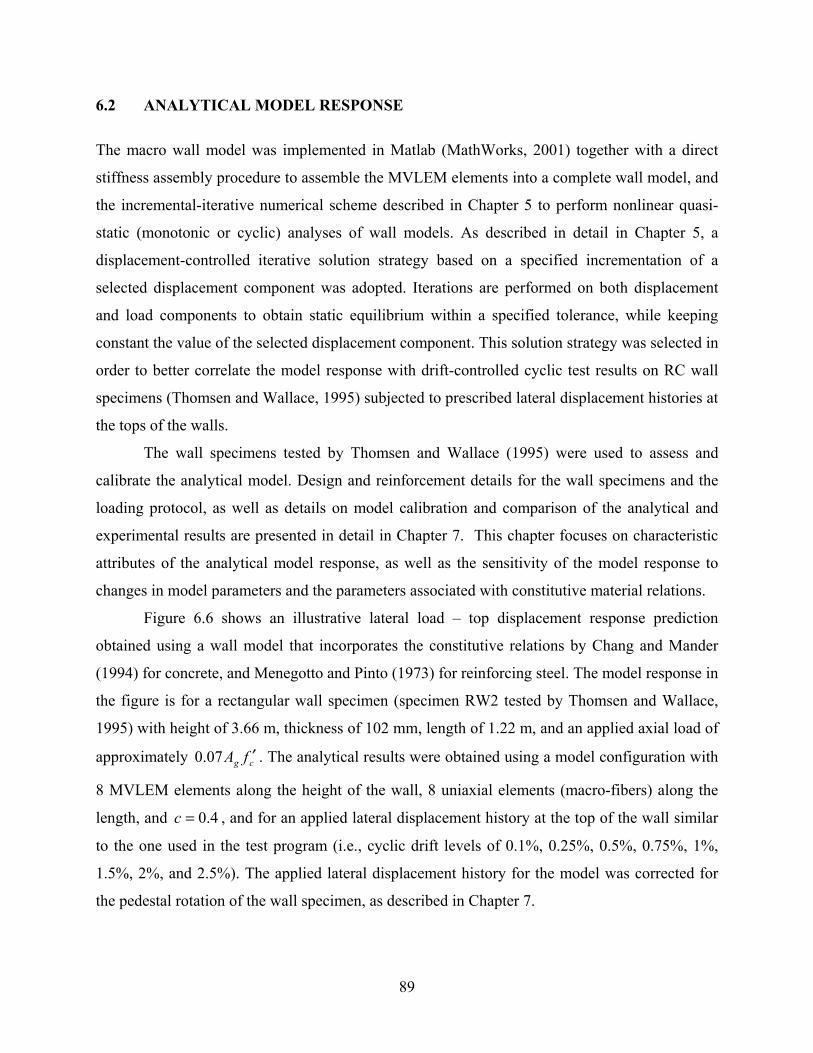
89
6.2 ANALYTICAL MODEL RESPONSE
The macro wall model was implemented in Matlab (MathWorks, 2001) together with a direct
stiffness assembly procedure to assemble the MVLEM elements into a complete wall model, and
the incremental-iterative numerical scheme described in Chapter 5 to perform nonlinear quasi-
static (monotonic or cyclic) analyses of wall models. As described in detail in Chapter 5, a
displacement-controlled iterative solution strategy based on a specified incrementation of a
selected displacement component was adopted. Iterations are performed on both displacement
and load components to obtain static equilibrium within a specified tolerance, while keeping
constant the value of the selected displacement component. This solution strategy was selected in
order to better correlate the model response with drift-controlled cyclic test results on RC wall
specimens (Thomsen and Wallace, 1995) subjected to prescribed lateral displacement histories at
the tops of the walls.
The wall specimens tested by Thomsen and Wallace (1995) were used to assess and
calibrate the analytical model. Design and reinforcement details for the wall specimens and the
loading protocol, as well as details on model calibration and comparison of the analytical and
experimental results are presented in detail in Chapter 7. This chapter focuses on characteristic
attributes of the analytical model response, as well as the sensitivity of the model response to
changes in model parameters and the parameters associated with constitutive material relations.
Figure 6.6 shows an illustrative lateral load – top displacement response prediction
obtained using a wall model that incorporates the constitutive relations by Chang and Mander
(1994) for concrete, and Menegotto and Pinto (1973) for reinforcing steel. The model response in
the figure is for a rectangular wall specimen (specimen RW2 tested by Thomsen and Wallace,
1995) with height of 3.66 m, thickness of 102 mm, length of 1.22 m, and an applied axial load of
approximately cg fA ′07.0 . The analytical results were obtained using a model configuration with
8 MVLEM elements along the height of the wall, 8 uniaxial elements (macro-fibers) along the
length, and 4.0=c , and for an applied lateral displacement history at the top of the wall similar
to the one used in the test program (i.e., cyclic drift levels of 0.1%, 0.25%, 0.5%, 0.75%, 1%,
1.5%, 2%, and 2.5%). The applied lateral displacement history for the model was corrected for
the pedestal rotation of the wall specimen, as described in Chapter 7.

90
-100 -60 -20 20 60 100
Top Displacement, Δtop (mm)
-200
-100
0
100
200
Late
ral L
oad,
Pla
t (k
N)
-2 -1 0 1 2Lateral Drift (%)
Pax= 0.07Ag f c'
Plat , Δtop
0 100 200 300 400Data Point Number
-4
-2
0
2
4
Δ top
(mm
)
Fig. 6.6 Load-displacement response predicted by analytical model
The analysis results clearly reflect actual characteristics of cyclic wall response, including
stiffness degradation, shape of the load-displacement hysteresis loops, plastic (residual)
displacements at zero load, and pinching. The model successfully captures the variation of the
neutral axis depth for a cyclic displacement history applied at the top of the wall, as shown in
Figure 6.7, which displays the predicted position of the neutral axis in the MVLE at the base of
the wall, normalized by the wall length. The distance from the centroid of the wall cross section
to the neutral axis approaches infinity when the lateral displacement (and thus rotation) of the
wall approaches zero, and reaches its local extrema or limit points (peaks and valleys) at peak
displacement (displacement reversal) points.
Figure 6.8 compares the average longitudinal strain histories predicted at the extreme
concrete fiber and at the centroid of the wall for the element at the base of the wall,
demonstrating the effect of applied displacement history and neutral axis migration on the
predicted strains. The longitudinal strains are not symmetric with respect to the zero strain axis;
and the strains predicted at the center of the wall are tensile for almost the entire loading history,
except for a range of small displacements (due to the presence of axial load).

91
0 100 200 300 400Data Point Number
-3
-2
-1
0
1
2
3
x N.A
. /l w
Peak Top Displacement Data PointsPositive DisplacementNegative Displacement
0.5
-0.5
xN.A.
lw
+- C.L.
(Wall Cross-Section)
Fig. 6.7 Predicted variation in position of neutral axis
0 100 200 300 400Data Point Number
-0.01
0
0.01
0.02
0.03
0.04
Long
itudi
nal S
train
, ε
Extreme FiberCentroid
Tension
Compression
Extreme Fiber
Centroid
(Wall Cross-Section)
Fig. 6.8 Predicted longitudinal strain histories
The MVLEM directly considers the effect of varying axial load on the wall response,
which although constant in this case, might vary in some cases (e.g., under dynamic loads such
as earthquakes). Figure 6.9 shows a comparison of the analytically predicted lateral load versus

92
top displacement responses for an applied axial load of zero and cg fA ′10.0 , clearly displaying
the significant impact of axial load on the wall response. Higher axial load results in larger
lateral load capacity of the wall at all drift levels, and a more pronounced pinching behavior
upon unloading to reloading in the opposite direction.
-100 -60 -20 20 60 100
Top Displacement (mm)
-200
-100
0
100
200
Late
ral L
oad
(kN
)
-2 -1 0 1 2Lateral Drift (%)
Pax = 0.10 Ag f c'
Pax = 0
Fig. 6.9 Effect of axial load on analytical response
The monotonic and quasi-static lateral load – top displacement responses predicted by the
wall model are compared in Figure 6.10(a). The model successfully simulates the cyclic strength
degradation associated with the Bauschinger’s effect observed in reinforcing steel. Figure
6.10(b) shows a comparison of sample monotonic and cyclic stress-strain relations for
reinforcing steel, generated by the constitutive model by Menegotto and Pinto (1973), in which
Bauschinger’s effect is illustrated. The monotonic stress-strain relation is essentially bilinear,
since the curvature parameter R is assigned a large value for monotonic loading ( 200 == RR );
whereas the parameters 1a and 2a (see Fig. 6.3) account for cyclic degradation of the curvature
parameter R , and thus allow modeling of the Bauschinger’s effect. This behavior is reflected in
the analytical lateral load – top displacement response of the wall shown in Figure 6.10(a).

93
-100 -60 -20 20 60 100
Top Displacement (mm)
-200
-100
0
100
200
Late
ral L
oad
(kN
)
-2 -1 0 1 2Lateral Drift (%)
MonotonicCyclic
(a) Monotonic and quasi-static load-displacement responses predicted by the model
-0.005 0 0.005 0.01 0.015 0.02 0.025 0.03 0.035
Strain, ε
-600
-400
-200
0
200
400
600
Stre
ss, σ
(M
Pa)
Monotonic, R0=20Hysteretic, R0=20 , a1=18.5 a2=0.0015
(b) Monotonic and hysteretic stress-strain response histories for reinforcing steel
Fig. 6.10 Monotonic and quasi-static responses

94
The monotonic load-displacement response of the wall produces lateral load capacities
larger than that of the cyclic response at all drift levels. This is because the monotonic stress-
strain relation of reinforcing steel generates higher stresses compared to the hysteretic stress-
strain relation, due to Bauschinger’s effect (Fig. 6.10(b)). The shape of the monotonic lateral
load – top displacement response predicted by the wall model resembles the shape of a typical
monotonic moment-curvature (moment-rotation) relation for a reinforced concrete cross section.
Figure 6.11 compares the analytical lateral load – top displacement response prediction
obtained using a model with the constitutive relation by Chang and Mander (1994) implemented
for concrete, with that obtained using the constitutive relation by Yassin (1994). The primary
shortcoming of the constitutive model by Yassin is the inability of the model to simulate gradual
gap closure due to progressive contact stresses within the cracks in concrete. Sudden crack
closure (see Fig. 6.5) results in a pronounced and overestimated pinching behavior (i.e.,
characteristic variation in section stiffness from unloading to reloading in the opposite direction)
for the wall. This is represented in Figure 6.11, where a sudden change in wall lateral stiffness is
observed when the constitutive model by Yassin (1994) is used. In contrast, the constitutive
model by Chang and Mander (1994) yields a progressive and gradual pinching behavior; that is,
the model by Chang and Mander successfully simulates the gradual closure of cracks (see Fig.
6.4) due to progressive contact stresses occurring across cracks.
As discussed in Chapter 7, the analytical model accurately represents the stiffness
degradation properties upon unloading and the wall pinching behavior (as well as other attributes
of cyclic wall response) observed in test results when the constitutive model by Chang and
Mander is used. Therefore, the constitutive model by Yassin was not used in any further studies.
However, the constitutive model by Yassin is a simple and widely used (e.g., OpenSees)
alternative, and can be efficiently used when accurate prediction of wall unloading and pinching
properties is of secondary concern. The two responses depicted in Figure 6.11 are not notably
different in the regions other than those associated with unloading and reloading in opposite
direction, although the shape of the monotonic compression and tension envelopes of the stress-
strain relations by Chang and Mander and Yassin are significantly different (compare Figs. 6.4
and 6.5). This highlights the fact that the analytical model response for the wall and loading
regime used in this study is not very sensitive to the shape of the envelopes used for modeling
the monotonic stress-strain behavior of concrete. The sensitivity of the model response to

95
constitutive material parameters, as well as model parameters, is investigated in the following
section.
-100 -60 -20 20 60 100
Top Displacement (mm)
-200
-100
0
100
200
Late
ral L
oad
(kN
)-2 -1 0 1 2
Lateral Drift (%)
Concrete Constitutive Models:Chang and Mander (1994)Yassin (1994)
Fig. 6.11 Analytical load-displacement response predictions obtained using different constitutive relations for concrete
6.3 PARAMETRIC SENSITIVITY STUDIES
It has been observed that in addition to the model parameters (number of macro wall elements
(m), number of uniaxial elements or macro-fibers within each element (n), and center of rotation
parameter (c), properties of the uniaxial hysteretic constitutive models defined for the materials
influence the analytical response predictions. The sensitivity of the results obtained with the
model to both model and material constitutive parameters is addressed in the following
subsections.
6.3.1 Material Constitutive Parameters
The MVLEM implemented in this study relates the predicted flexural response directly to
material behavior without incorporating any additional empirical relations, as done in prior

96
studies (Fischinger et al., 1990; Fajfar and Fischinger, 1990; Fischinger et al., 1991, 1992). It has
been observed that the predicted load-displacement response is, as expected, influenced by the
properties of the stress-strain relations implemented for the longitudinal reinforcement and the
unconfined and confined concrete; therefore, it is necessary to understand how variations in the
material constitutive laws influence the results obtained using the model, particularly in the
context of performance-based seismic design.
The material constitutive parameters associated with the implemented steel stress-strain
law are the modulus of elasticity (E0), the yield stress (σy), the strain-hardening ratio (b) and the
parameters (R0, a1 and a2) influencing the cyclic curvature of the transition curve between the
elastic and yield asymptotes. Values for E0, σy, and b are obtained from monotonic stress-strain
tests conducted on bare rebar specimens, allowing for a reliable calibration. However, the values
for the yield stress (σy) and strain-hardening ratio (b) in tension should be modified to consider
the tension-stiffening effect on the reinforcing bars, and can be calibrated for average values
using relations such as those proposed by Belarbi and Hsu (1994). Figure 6.12 illustrates the
sensitivity of the analytical lateral load – top displacement response to the value of the tensile
yield stress (σy) selected for reinforcing steel. Figure 6.12(a) shows sample stress-strain histories
generated by the steel constitutive model for two different values selected for the tensile steel
yield stress, whereas the corresponding lateral load – top displacement responses of the wall
specimen predicted by the analytical model are compared in Figure 6.12(b). As expected,
selecting a higher level of yield stress for steel in tension results in a larger prediction of the wall
lateral load capacity at all drift levels. Figure 6.13 shows the sensitivity of the model response to
the strain-hardening ratio (b) of steel in tension. Selection of a larger strain-hardening ratio value
yields a larger post-yield lateral stiffness of the wall, and thus larger lateral load capacities at
post-yield drift levels (i.e., 0.5%–2% drift).
The calibration of parameters R0, a1 and a2 (accounting for the cyclic degradation of the
curvature coefficient R) requires cyclic test results, which are not commonly available. Figure
6.14(a) shows sample stress-strain histories generated by the steel constitutive model for two
different sets of values for parameters R0, a1, and a2, calibrated by prior researchers (Filippou et
al., 1994; Elmorsi et al., 1998) based on cyclic test results on reinforcing steel bars.
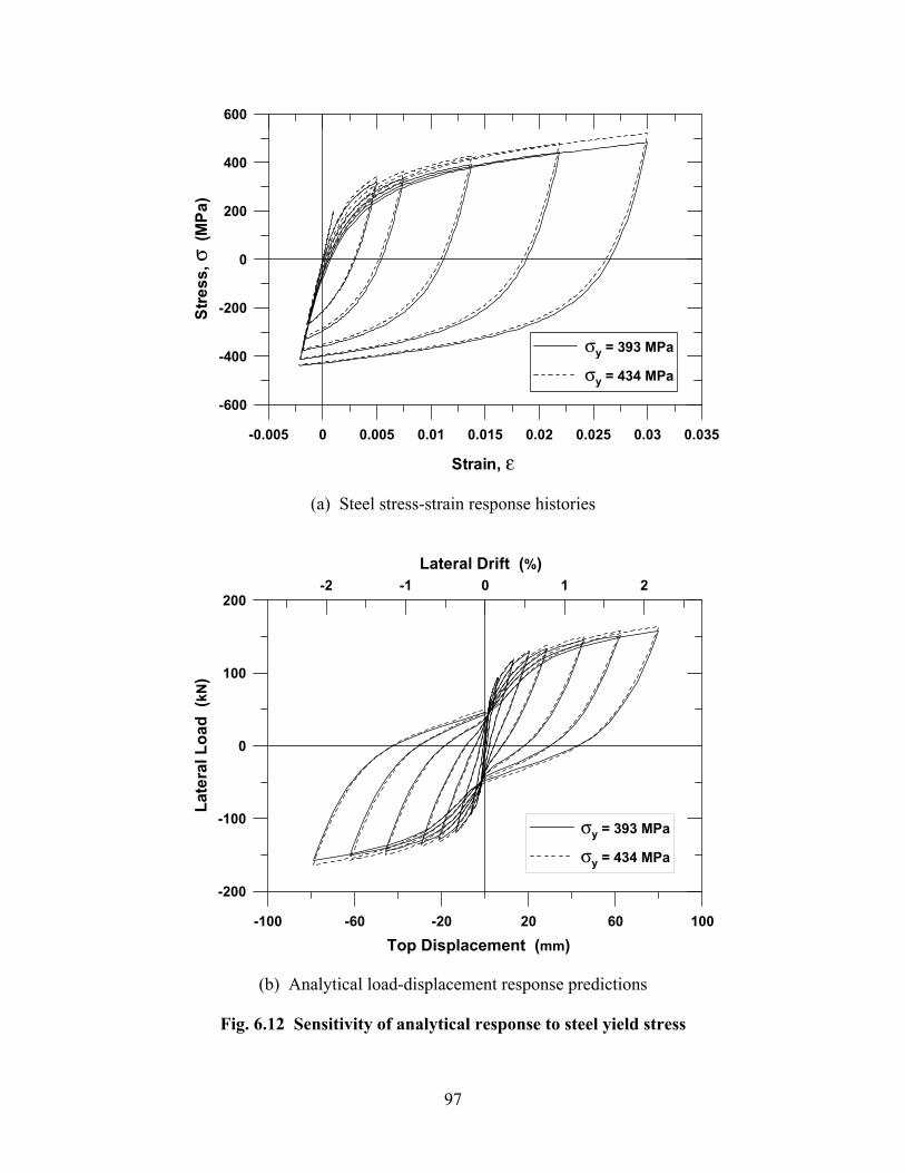
97
-0.005 0 0.005 0.01 0.015 0.02 0.025 0.03 0.035
Strain, ε
-600
-400
-200
0
200
400
600
Stre
ss, σ
(M
Pa)
σy = 393 MPa
σy = 434 MPa
(a) Steel stress-strain response histories
-100 -60 -20 20 60 100
Top Displacement (mm)
-200
-100
0
100
200
Late
ral L
oad
(kN
)
-2 -1 0 1 2Lateral Drift (%)
σy = 393 MPa
σy = 434 MPa
(b) Analytical load-displacement response predictions
Fig. 6.12 Sensitivity of analytical response to steel yield stress

98
-0.005 0 0.005 0.01 0.015 0.02 0.025 0.03 0.035
Strain, ε
-600
-400
-200
0
200
400
600
Stre
ss, σ
(M
Pa)
b = 0.02b = 0.03
(a) Steel stress-strain response histories
-100 -60 -20 20 60 100
Top Displacement (mm)
-200
-100
0
100
200
Late
ral L
oad
(kN
)
-2 -1 0 1 2Lateral Drift (%)
b = 0.02b = 0.03
(b) Analytical load-displacement response predictions
Fig. 6.13 Sensitivity of analytical response to steel strain-hardening ratio

99
-0.005 0 0.005 0.01 0.015 0.02 0.025 0.03 0.035
Strain, ε
-600
-400
-200
0
200
400
600
Stre
ss, σ
(M
Pa)
R0=20 a1=18.5 a2=0.0015R0=20 a1=18.5 a2=0.15
(a) Steel stress-strain response histories
-100 -60 -20 20 60 100
Top Displacement (mm)
-200
-100
0
100
200
Late
ral L
oad
(kN
)
-2 -1 0 1 2Lateral Drift (%)
R0=20 a1=18.5 a2=0.0015R0=20 a1=18.5 a2=0.15
Peak Top Displacement Data Points,
(b) Analytical load-displacement response predictions
Fig. 6.14 Sensitivity of analytical response to hysteretic parameters for steel

100
The analytical lateral load – top displacement responses of the wall specimen predicted
by the MVLEM using the specified values for the material parameters (R0, a1, and a2 in Fig.
6.14(a)) are shown in Figure 6.14(b). The lateral load capacity of the wall is significantly
influenced by these hysteretic parameters; primarily in the region where the steel is not subjected
to high post-yield strains (e.g., 0.5%–0.75% drift). Cyclic degradation of the lateral stiffness
during unloading and plastic (residual) displacements at zero lateral load also depend on the
selection of these parameters, as shown in Figure 6.14(b).
The material parameters associated with the implemented concrete stress-strain relation
are the monotonic (envelope) parameters (Ec, 'cf or tf , '
cε or tε , r) and the hysteretic
parameters ( fΔ , εΔ , plE , secE ) defined for compression and tension (Fig. 4.13). The empirical
relations used to define these parameters for monotonic and cyclic compression (for both
confined and unconfined concrete) were validated by Chang and Mander (1994) using extensive
experimental data from column tests. The relations defining the parameters for cyclic tension,
however, were obtained using limited experimental data. Furthermore, the observed tensile
strength and stress-strain properties of concrete depend strongly on the testing conditions (Chang
and Mander, 1994) and considerable scatter is observed in the data scattering, making it difficult
to assign values for the parameters that define the concrete tensile stress-strain relation.
Therefore, the sensitivity of the predicted wall response to concrete stress-strain parameters
investigated here focuses on concrete tensile strength and the hysteretic parameters related to
cyclic tension, as well as because model results are less sensitive to variations in the parameters
describing the behavior of concrete in compression.
Figure 6.15 illustrates how the predicted monotonic and cyclic lateral load – top
displacement responses of the wall specimen (with applied axial load 7% of axial load capacity)
are influenced by selection of the tensile strength (peak tensile stress) for concrete ( tf ). The
strain at peak tensile stress ( tε ) was varied proportionally with the peak tensile stress, while the
shape parameter r was kept constant. Neglecting the contribution of concrete in tension results in
a lower prediction of the wall lateral stiffness and a slightly lower prediction of the wall lateral
strength compared with results that include the contribution of concrete in tension. Furthermore,
variation in the assumed tensile strength for concrete influences the cyclic properties of the
predicted response, as shown in Figure 6.15.

101
0.1 0.25 0.5 1 20 0.48 0.73 0.93 1.06 1.18
0.31 0.58 0.82 1.00 0.11 1.220.5 0.66 0.90 1.07 1.16 1.26
-100 -60 -20 20 60 100
Top Displacement (mm)
-200
-100
0
100
200
Late
ral L
oad
(kN
)
-2 -1 0 1 2Lateral Drift (%)
ft = 0ft = 0.31√ fc
' (MPa)
ft = 0.5 √ fc' (MPa)
Monotonic
Cyclic Lateral Drift (%)
f t / √
f c'
Lateral Load (kN)/132
Fig. 6.15 Effect of concrete tensile strength on analytical response
The hysteretic parameters associated with the cyclic concrete stress-strain law in tension
are the plastic stiffness ( +plE ) and secant stiffness ( +
secE ) upon unloading from, and stress and
strain offsets ( +Δf and +Δε ) upon return to the tension envelope (Fig. 4.13). The predicted wall
response is not notably influenced by the stress and strain offsets, since the offsets influence the
shape of the stress-strain curve within a very small range of tensile stresses. On the other hand,
the predicted wall response is significantly influenced by values selected for the plastic and
secant stiffnesses for unloading in tension because these parameters control the starting strain
and initial slope for the gap closure region of the concrete stress-strain law. Figure 6.16(a)
compares sample stress-strain histories generated by the constitutive relation for concrete with
the original expression derived by Chang and Mander (1994) for the plastic stiffness in tension
( +plE ) and an illustrative value of zero, and Figure 6.16(b) compares the corresponding predicted
load-displacement responses of the wall obtained using 17 MVLEM elements along the wall
height (8 of the MVLEM elements stacked along the bottom one fourth of the wall height and
the rest distributed uniformly over the wall height) with 22 uniaxial elements along the wall
length, and 4.0=c . The figures reveal that the shape of the unloading and reloading curves of
the predicted load-displacement response is governed by the selection of the value for plastic

102
stiffness ( +plE ), which together with the secant stiffness ( +
secE ), governs the progressive gap
closure properties (i.e., pinching) of the concrete stress-strain relation. Using a value of zero for +plE results in an abrupt change in the lateral stiffness of the wall from unloading to reloading in
the opposite direction, and thus a much more pronounced pinching behavior (similar to the cyclic
response in Figure 6.15, when concrete tensile stresses are neglected, i.e., 0=tf ; and thus the
plastic stiffness for unloading in tension is zero), whereas implementing the original relation
imposes a more gradual change in the lateral stiffness of the wall. However, the variation in the
pinching behavior does not change the lateral strength and stiffness of the wall at peak top
displacement (displacement reversal) points, since the enforced peak displacements of the wall
are increasing for successive loading cycles.
Similar behavior is observed in the analytically predicted position of the neutral axis and
the predicted longitudinal strains. Figure 6.16(c) shows the position of the neutral axis predicted
in the MVLE at the base of the wall obtained by using the two different expressions for the
tensile plastic stiffness ( +plE ). The neutral axis positions reach the same local limit values at peak
displacement data points, and variation between the two cases is enhanced as the displacement
(or rotation) of the wall approaches zero. Finally, Figure 6.16(d) illustrates the influence of the
plastic stiffness on predicted longitudinal strain histories for the element at the base of the wall.
For the two cases investigated, the strains at both the extreme fiber and centroid are identical at
peak displacement data points; however, noticeable variation is observed in the strains (more
distinctly at the centroid) as the wall displacement approaches zero.
The variation in the unloading and reloading regions of the predicted response (Fig.
6.16(b)) has only a marginal effect on the energy dissipation capacity of the wall model.
Calculating the hysteretic energy dissipation capacity for the plots in Figure 6.16(b) normalized
by that of a bilinear lateral load – top displacement relation yields values of 0.66 for the response
obtained by using the relation for the tensile plastic stiffness defined by Chang and Mander
(1994), and 0.64 using a zero value for the tensile plastic stiffness.
Variation in the secant stiffness defined for concrete in tension ( +secE ), influences wall
response in approximately the same way as changes in the plastic stiffness ( +plE ).

103
Strain, ε
Stre
ss, σ
Epl+ (Chang and Mander, 1994)
Epl+ = 0
O
Not to scale
Compression
(εc0+εt,ft)
( εun+
, f un+ )
( εpl+
,0)
( εun-
, f un- )
(εc0,0)( εpl
-
,0)Tension
( εc ' , f c
' )
(a) Concrete stress-strain response histories
-100 -60 -20 20 60 100
Top Displacement (mm)
-200
-100
0
100
200
Late
ral L
oad
(kN
)
-2 -1 0 1 2Lateral Drift (%)
Epl+
Epl+ = 0
Bilinear Force-DisplacementRelation
(b) Predicted load-displacement responses
Fig. 6.16 Effect of concrete tensile plastic stiffness on analytical response

104
0 100 200 300 400Data Point Number
-1
-0.5
0
0.5
1
x N.A
. /l w
Epl+
Epl+ = 0
Peak top displacement data points
(c) Predicted position of the neutral axis
0 100 200 300 400Data Point Number
-0.01
0
0.01
0.02
0.03
0.04
Long
itudi
nal S
train
, ε
Strain at Extreme Fiber Epl
+
Epl+ = 0
Strain at Centroid Epl
+
Epl+ = 0
Peak top displacement data points
Tension
Compression
(d) Predicted longitudinal strain histories
Fig. 6.16 (cont’d.)

105
The empirical relations defined by Chang and Mander for the plastic stiffness and secant
stiffness in tension were obtained from limited experimental data (Yankelevsky and Reinhardt,
1987) with imposed tensile strains reaching a value of approximately 0.003. However, the tensile
strains in walls are likely to reach much larger values (e.g., 0.035 in this example); thus, using
the Chang and Mander empirical relations for such high levels of tensile strain may be
inappropriate. Calibration of these two hysteretic parameters for a broader range of tensile
strains, and also accounting for the tension-stiffening effect, would refine the modeling of the
gap closure region of the concrete stress-strain behavior, and the prediction of the wall pinching
behavior. Fortunately, the concrete model proposed by Chang and Mander (1994) provides a
flexible approach that allows recalibration of such parameters to control gap closure properties of
concrete for an improved overall representation of wall force-deformation relations.
It has been observed that the model results are less sensitive to variation in the parameters
defining the monotonic and hysteretic stress-strain relation for concrete in compression, provided
that the values used for the parameters are within reasonable range such as those obtained by
using the empirical relations recommended by Chang and Mander. The empirical relations relate
the parameters for compression (i.e., modulus of elasticity Ec, strain at peak compressive stress 'cε , parameter r defining the shape of the compression envelope (Eqs. 4.49–4.51), and hysteretic
parameters for compression including stress and strain offsets ( −Δf and −Δε ), and unloading
plastic stiffness and secant stiffness ( −plE and −
secE )) to the value selected for the unconfined
compressive strength (peak unconfined compressive stress, 'cf ) of concrete (Eqs. 4.78–4.81).
The governing parameter 'cf can be feasibly calibrated with monotonic stress-strain tests
conducted on concrete specimens (e.g., 152.5 x 305 mm standard cylinders).
Figure 6.17 compares the lateral load – top displacement responses predicted by the wall
model for a 25% variation in the unconfined compressive strength ( 'cf ) of concrete. The
responses are not noticeably different, although all of the parameters associated with the
monotonic and hysteretic parameters of the constitutive stress-strain relation for concrete in
compression (Ec, 'cε , r, −Δf , −Δε , −
plE , −secE ) are varied based on the value selected for '
cf . The
result indicates that, for the wall properties and loading protocol used in this study, the model
response is insensitive to either the value of the compressive strength selected for concrete, or
any of the parameters associated with the shape of the monotonic or hysteretic stress-strain
branches for concrete in compression as long as there is no extreme variation in the assumed

106
compressive strength of concrete and the values selected for the monotonic and hysteretic
constitutive parameters for concrete in compression are within the range of typically expected
variation.
-100 -60 -20 20 60 100
Top Displacement (mm)
-200
-100
0
100
200
Late
ral L
oad
(kN
)
-2 -1 0 1 2Lateral Drift (%)
fc'
= 42 MPa
fc'
= 31.5 MPa
Fig. 6.17 Sensitivity of analytical response to concrete compressive strength and associated parameters
The wall model, together with the nonlinear solution strategy implemented in this study,
can simulate the strength degradation associated with the descending (post-peak) branch of the
concrete stress-strain constitutive model. This is shown in Figure 6.18, where the analytical
lateral load – top displacement responses are compared for an extreme (50%) variation in the
unconfined compressive strength of concrete. As observed in the figure, the concrete
compressive strength does not significantly influence the lateral load capacity of the wall prior to
strength degradation due to the post-peak branch of the concrete stress-strain relation
(progressive concrete crushing). However, it influences the lateral drift level at which strength
degradation is initiated.
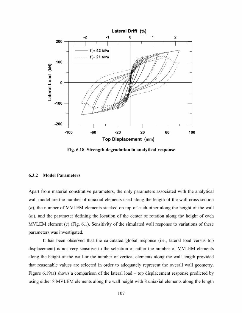
107
-100 -60 -20 20 60 100
Top Displacement (mm)
-200
-100
0
100
200
Late
ral L
oad
(kN
)
-2 -1 0 1 2Lateral Drift (%)
fc'
= 42 MPa
fc'
= 21 MPa
Fig. 6.18 Strength degradation in analytical response
6.3.2 Model Parameters
Apart from material constitutive parameters, the only parameters associated with the analytical
wall model are the number of uniaxial elements used along the length of the wall cross section
(n), the number of MVLEM elements stacked on top of each other along the height of the wall
(m), and the parameter defining the location of the center of rotation along the height of each
MVLEM element (c) (Fig. 6.1). Sensitivity of the simulated wall response to variations of these
parameters was investigated.
It has been observed that the calculated global response (i.e., lateral load versus top
displacement) is not very sensitive to the selection of either the number of MVLEM elements
along the height of the wall or the number of vertical elements along the wall length provided
that reasonable values are selected in order to adequately represent the overall wall geometry.
Figure 6.19(a) shows a comparison of the lateral load – top displacement response predicted by
using either 8 MVLEM elements along the wall height with 8 uniaxial elements along the length

108
of the wall or by using 17 MVLEM elements along the wall height (8 of the MVLEM elements
stacked along the bottom one fourth of the height where the inelastic deformations are expected,
and the rest distributed uniformly over the wall height) with 22 uniaxial elements along the wall
length. The comparison indicates that increasing the number of vertical line elements or the
number of MVLEM elements does not significantly change the prediction of the global response
(i.e., lateral load versus top displacement); however, use of more elements is valuable in terms of
obtaining more detailed information on local behavior, such as the state of stress and strain or
moment curvature response at a given location. For example, results shown in Figure 6.19(b)
compare the average longitudinal strain histories predicted at the extreme concrete fiber and the
centroid of the wall in the MVLE at the base of the two wall model configurations used for the
plots in Figure 6.19(a) ( 8=n , 8=m and 17=n , 22=m ). Using more MVLEs over the height
of the wall allows for an improved local prediction of the strains, although the results obtained
using the “rough” model ( 8=n , 8=m ) are quite good. As well, using more uniaxial elements
along the wall length allows for a more refined description of the wall cross section. Therefore,
the model incorporates the flexibility to choose how much detail is desired in the analytical
results.
The sensitivity of analysis results to the parameter defining the location of the center of
rotation along the height of each MVLEM element (c) is illustrated in Figure 6.20. Figure
6.20(a) compares the predicted lateral load – top displacement (global) response by using a wall
model with 8 MVLEM elements (and 8 uniaxial elements) for a value of 4.0=c (recommended
by Vulcano et al., 1988) and an illustrative extreme value of 0.0=c (center of rotation at the
bottom of each MVLEM element). Decreasing the value of parameter c leads to a higher
prediction of rotations and lateral displacements of the wall, resulting in a slightly lower
prediction of the wall strength and lateral stiffness. However, this extreme variation in parameter
c does not influence the characteristic shape of the load-displacement response significantly. As
proposed by Fischinger et al. (1990), stacking more wall elements along wall height (especially
in the region where inelastic deformations are expected) reduces the change in curvature within
each element, thus diminishing the influence of the parameter c on the response. Figure 6.20(b)
compares the predicted global wall response for 4.0=c and 0.0=c using a wall model with 17
MVLEM elements with 8 of the elements stacked along the bottom one fourth of the wall height.
The two responses are very similar.

109
-100 -60 -20 20 60 100
Top Displacement (mm)
-200
-100
0
100
200
Late
ral L
oad
(kN
)
-2 -1 0 1 2Lateral Drift (%)
n = 8, m = 8n = 17, m = 22
(a) Lateral load – top displacement responses
0 100 200 300 400Data Point Number
-0.01
0
0.01
0.02
0.03
0.04
0.05
Long
itudi
nal S
train
, ε
Strain at Extreme Fibern = 8, m = 8n = 17, m = 22
Strain at Centroid n = 8, m = 8n = 17, m = 22
Tension
Compression
(b) Longitudinal strain histories in the MVLE at the base of the wall
Fig. 6.19 Sensitivity of response to number of MVLEM and uniaxial elements

110
-100 -60 -20 20 60 100
Top Displacement (mm)
-200
-100
0
100
200
Late
ral L
oad
(kN
)
-2 -1 0 1 2Lateral Drift (%)
n = 8 , m = 8c = 0.4c = 0.0
(a) Analytical model with 8 MVLEM elements and 8 uniaxial elements
-100 -60 -20 20 60 100
Top Displacement (mm)
-200
-100
0
100
200
Late
ral L
oad
(kN
)
-2 -1 0 1 2Lateral Drift (%)
n = 17 , m = 22c = 0.4c = 0.0
(b) Analytical model with 17 MVLEM elements and 22 uniaxial elements
Fig. 6.20 Sensitivity of response to center of rotation parameter c

111
6.4 SUMMARY
This chapter demonstrates the effectiveness of the present analytical model in simulating the
behavioral features associated with the inelastic response of slender RC structural walls. The
attributes of the responses obtained using the analytical model were studied. Variations of model
and material parameters were investigated to identify the sensitivity of analytically predicted
global and local wall responses to changes in these parameters as well as to identify which
parameters require the greatest care with respect to calibration.
Based on analysis results, it was verified that the MVLEM captures important response
characteristics associated with cyclic behavior of slender reinforced concrete structural walls
governed by flexure. The analytical model is able to simulate important behavioral features
including shifting of the neutral axis along the wall cross section, and the effect of fluctuating
axial force, which are commonly ignored in simple models. Characteristics of the cyclic
response, including stiffness degradation and strength deterioration, hysteretic shape, and
pinching behavior are clearly captured in the analysis results.
The modeling approach adopted in this study involves implementing refined hysteretic
uniaxial stress-strain laws instead of simplified (ad hoc) force-deformation rules to track
nonlinear responses. This allows the designer to relate analytical responses directly to physical
material behavior and provides a more robust modeling approach, where model improvements
result from improvement in constitutive models and refinement in the spatial resolution of the
discrete model. The constitutive relations implemented in the wall model provide a direct and
flexible approach to incorporate important material behavioral features (e.g., Bauschinger’s
effect in reinforcing steel, hysteretic behavior of concrete in continuous compression and tension,
progressive gap closure, tension-stiffening effect) into the analysis. It has been observed that the
model responses are sensitive not only to material parameters associated with the monotonic
stress-strain behavior, but also significantly by variation in the hysteretic parameters defined for
the steel (R0, a1, a2) and for concrete in tension ( +plE , +
secE ). Thus, careful calibration of these
parameters is important for an improved prediction of the cyclic wall response.
Overall, the macroscopic wall model presented here provides a flexible platform to assess
the influence of various material and behavioral features in the nonlinear responses of slender
RC structural walls. Details on calibration of the model and correlation of predicted responses

112
with extensive test results, at both global and local response levels, are presented in the following
chapter.

7 Flexural Modeling — Experimental Calibration and Verification
This chapter presents detailed information on the calibration of the analytical macro-model and
comparison of model results with experimental results for slender reinforced concrete walls.
Comprehensive correlation studies were conducted to compare the analytically predicted and
experimentally observed behavior of slender RC walls with rectangular and T-shaped cross
sections at various response levels by processing the test measurements to allow for a direct
comparison of the predicted and measured flexural responses. Comparisons not only allow for a
better understanding of the inelastic behavior of RC walls, but also identify model capabilities as
well as ways to improve the model.
7.1 OVERVIEW OF EXPERIMENTAL STUDIES
The wall specimens tested by Thomsen and Wallace (1995, 2003) were used to calibrate and
assess the analytical model. Experimental results were obtained for four, approximately quarter-
scale wall specimens. The walls tested included two walls with rectangular cross sections (RW1,
RW2), and two walls with T-shaped cross sections (TW1, TW2), with the primary variable in the
test program being the level of detailing provided at the wall boundaries. A brief overview of
these studies is provided in the following sections, with more detailed information concerning
the wall tests presented by Thomsen and Wallace (1995, 2003).
7.1.1 Test Specimen Information
The walls were 3.66 m tall and 102 mm thick, with web and flange lengths of 1.22 m (Fig. 7.1).
Floor slabs were provided at 0.915 m intervals over the height of the T-shaped walls (consisting
of four stories).

114
(a) Rectangular Wall (b) T-shaped Wall
Fig. 7.1 RC wall specimens tested by Thomsen and Wallace (1995)
GROUND LEVEL
FIRST FLOOR
SECOND FLOOR
THIRD FLOOR
FOURTH FLOOR
0.69 m
3.66 m
1.22 m
1.93 m
Fig. 7.2 Profile view of specimen RW2 showing placement of reinforcement

115
Typical material properties were selected for design, i.e., cf ′ = 27.6 MPa and yσ = 414
MPa. The wall specimens were proportioned based on a prototype building designed using the
strength requirements of the Uniform Building Code (1994); however, detailing requirements at
the boundaries of the wall specimens were evaluated using the displacement-based design
approach presented by Wallace (1994, 1995). Longitudinal reinforcement at wall boundaries
consisted of 8 - #3 (db = 9.53 mm) bars, whereas uniformly distributed web reinforcement
consisted of two curtains of deformed #2 (db = 6.35 mm) bars.
Transverse reinforcement at wall boundaries comprises 4.76 mm diameter smooth wire
that was annealed to give material properties similar to those of Grade 60 (414 MPa) reinforcing
steel. Well-detailed boundary elements were provided at the edges of the walls over the bottom
1.22 m ( wl ) of each wall. A capacity design approach was used to avoid shear failure, and
favorable anchorage conditions existed for the vertical reinforcement anchored with 90-degree
hooks within the pedestal at the base of the walls (Fig. 7.2). Sample reinforcing details for a
rectangular wall specimen RW2 and for a T-shaped wall specimen TW2 (at wall base levels) are
shown in Figure 7.3.
7.1.2 Materials
The compressive strength of concrete used for design of the wall specimens was 27.6 MPa;
however, concrete compressive strengths at the time of testing ranged from 28.7 to 58.4 MPa,
with mean compressive strengths at the base of the wall specimens (0–0.91 m) of approximately
32.8 MPa for the specimens RW1 and TW1, and 42.8 MPa for the specimens RW2 and TW2.
Peak compressive stress was reached for a cylinder compressive strain of approximately 0.002
for all specimens. Figure 7.4 plots the stress-strain relations, measured at the time of testing
using 152.4 mm x 304.8 mm standard cylinder specimens, of the concrete used in the
construction of the walls.
Three different types of reinforcing steel were used in the tests: (1) typical Grade 60 (414
MPa), deformed #3 (db = 9.53 mm) bars as longitudinal reinforcement, (2) deformed #2 (db =
6.35 mm) bars uniformly distributed web steel, and (3) 4.76 mm diameter smooth wire as
transverse reinforcement in the boundary regions. Figure 7.5 plots the measured longitudinal
stress-strain relations for each type of reinforcement. The #3 (db = 9.53 mm) bars used as

116
longitudinal boundary reinforcement had typical Grade 60 properties; however, the other two
types of steel exhibited some atypical behavior. The deformed #2 (db = 6.35 mm) bars used as
uniformly distributed web reinforcement had a yield stress of approximately 448 MPa; however,
they did not exhibit a well-defined yield plateau. The 4.76 mm diameter smooth wire was
annealed to lower the yield stress from approximately 552 MPa to approximately 448 MPa;
however, the strain-hardening region of the annealed wire was relatively flat (Fig. 7.5).
1219 mm
19 mm 19 mm3 @ 51 mm 153 mm 3 @ 191 mm 153 mm 3 @ 51 mm
64 mm
19 mm
19 mm
102 mm
#2 bars (db=6.35 mm) Hoops (db=4.76 mm)8 - #3 bars(db=9.53 mm) @ 191 mm @ 76 mm
(a) Specimen RW2
19 mm 19 mm
3 @ 51 mm153 mm 3 @ 191 mm 153 mm
3 @ 51 mm
64 mm
19 mm
19 mm
1219 mm
3 @ 140 mm
102 mm
4 @ 102 mm
19 mm
102 mm
19 mm
3 @ 51 mm
102 mm
1219 mm
8 - #3 bars(db=9.53 mm)
#2 bars (db=6.35 mm) @ 191 mm
Hoops (db=4.76 mm)@ 76 mm
#2 bars (db=6.35 mm) @ 140 mm
2 - #2 bars (db=6.35 mm)
Hoops and cross-ties (db=4.76 mm)@ 38 mm
8 - #3 bars(db=9.53 mm)
Hoops (db=4.76 mm)@ 32 mm
(b) Specimen TW2
Fig. 7.3 Wall cross-sectional views

117
0 0.001 0.002 0.003 0.004
Strain
0
10
20
30
40
50
Stre
ss (M
Pa)
RW1, TW11st Story2nd Story
(a) Specimens RW1 and TW1
0 0.001 0.002 0.003 0.004
Strain
0
10
20
30
40
50
Stre
ss (M
Pa)
RW2, TW21st Story2nd Story3rd Story4th Story
(a) Specimens RW2 and TW2
Fig. 7.4 Measured concrete stress-strain relations

118
0 0.02 0.04 0.06 0.08 0.1
Strain
0
100
200
300
400
500
600
700
Stre
ss (
MPa
)
#3 rebar#2 rebar4.76 mm wire
Fig. 7.5 Measured steel stress-strain relations
7.1.3 Testing Apparatus
The wall specimens were tested in an upright position in the Structural Engineering Research
Laboratory (SERL) at Clarkson University. Figure 7.6 shows a schematic of the overall test
setup. A photograph of the setup is shown in Figure 7.7. The walls were rigidly mounted to the
strong floor through the use of eight 32 mm diameter high-strength steel tie-down rods, passing
through the specimens’ pedestals.
A specially fabricated load transfer assembly was used to transfer both axial and lateral
loads to the wall specimen. The steel assembly was made of back-to-back channel sections (C-
12x68’s) welded together with a 19 mm gap between them to allow the post-tensioning strands to
pass through. The load transfer assembly was attached to the wall specimen using 25 mm
diameter threaded rods that were cast integrally with the fourth story of each specimen. Six
threaded rods were used to attach the assembly to the rectangular walls, whereas nine rods were
used on the T-shaped walls. Axial stress was applied by hydraulic jacks mounted on top of the
load transfer assembly (Fig. 7.8). Post-tensioning strands were anchored in the specimen’s
pedestal and run up through the back-to-back channels and through the hollow jacks. An axial
stress of approximately cg fA ′10.0 was maintained throughout the duration of each test.

119
High-StrengthPost-Tensioning
Cables
Hydraulic Actuator
Load Cell
Hydraulic Jacks
Reaction Wall
Strong Floor
Pedestal
Wall Specimen
1.22 m
3.66 m
Load CellsPancake
686 mmPedestalTie-Downs
305 mm
Cable AnchoredHere
B.T.B. Channels
Clip Angles
Rectangular
Fig. 7.6 Schematic of test setup (Thomsen and Wallace, 1995)
Fig. 7.7 Photograph of test setup (Thomsen and Wallace, 1995)

120
Fig. 7.8 Load transfer assembly
Cyclic lateral loads were applied to the walls by a 556 kN hydraulic actuator that was
mounted horizontally to a reaction wall approximately 3.81 m above the base of the walls. Both
ends of the actuator used a pin connection that allowed the actuator to rotate freely in the vertical
plane throughout the tests (Fig. 7.9).
Fig. 7.9 Hydraulic actuator
Out-of-plane support was provided during each test to provide stability. A steel truss was
placed between the top of the wall specimens and the reaction wall parallel to the specimen’s
web, allowing free movement parallel to the load direction but preventing perpendicular motion.

121
In this manner, twisting of the wall was eliminated and out-of-plane restraint was provided. The
support system also did not inhibit vertical wall movement.
7.1.4 Instrumentation and Data Acquisition
Instrumentation was used to measure displacements, loads, and strains at critical locations for
each wall specimen (Fig. 7.10). Wire potentiometers, linear potentiometers, and linear variable
differential transducers (LVDTs) were used to measure displacement response. Load cells were
used to measure axial and lateral loads, and strain gages were used to measure strains in the
concrete and the reinforcing steel.
Wire Potentiometers(horizontal displacement)
Wire Potentiometers (X configuration)
Wire Potentiometers(vertical displacement)
LVDT's
Concrete Strain Gages
Steel Strain Gage Levels
Ground Level
First Floor
Second Floor
Third Floor
Fourth Floor
Linear Potentiometers (Pedestal Movement)
25 203
229 229
203
152
25
152
229
533
38
914
686
914.5
914.5
914.5
914.5
Rigid Reference Frame
92
1219
1930
RW2
95
76
51
Units in mm
(a) Specimen RW2
Fig. 7.10 Instrumentation on wall specimens

122
Wire Potentiometers(horizontal displacement)
Wire Potentiometers (X configuration)
Wire Potentiometers(vertical displacement)
LVDT's
Concrete Strain Gages
Steel Strain Gage Levels
Ground Level
First Floor
Second Floor
Linear Potentiometers (Pedestal Movement)
229
533
38
914
686
914.5
914.5
457 457 25Rigid Reference Frame
128152
92
1676
1219
178203178
25
LVDT's
TW2
108 32
152
457 457 128 25
76
51
Units in mm
(b) Specimen TW2
Fig. 7.10 (cont’d.) Instrumentation on wall specimens
A rigid steel reference frame was mounted to the strong floor at the end of the wall
specimen to provide a location for instrumentation to be attached. Four wire potentiometers were
mounted to the reference frame to measure lateral displacements at 0.91 m intervals (at floor
levels) over the wall height. A linear potentiometer also was mounted horizontally on the
pedestal to measure any horizontal slip of the pedestal along the strong floor. Two additional
linear potentiometers were mounted vertically at each end of the pedestal to measure rotation
caused by uplift of the pedestal from the strong floor (Figs. 7.10–7.11).
Axial loads were measured using hollow pancake load cells and lateral cyclic loads were
measured using a 667 kN load cell mounted in series with the hydraulic actuator. The load cell
used to measure lateral loads can be seen in Figure 7.8.

123
Shear deformations were measured through the use of wire potentiometers mounted on
the bottom two stories (in an “X” configuration) of each specimen (Fig. 7.10). Figure 7.12 shows
a photograph of the wire potentiometers used to measure shear deformations on specimen RW2.
Axial (vertical) displacements at the wall boundaries were measured using two wire
potentiometers mounted between the base and first-story level at each end of the walls (Fig.
7.10). Wall base rotations were obtained by taking the difference in the axial displacements
measured by the two wire potentiometers and dividing the difference in relative axial
displacements by the distance between the potentiometers.
Linear variable differential transducers (LVDTs) were mounted vertically (Figs. 7.10,
7.13), over a gage length of 229 mm, at various locations along the web and flange of each wall
so that axial strains and section curvatures could be calculated. The rectangular walls were
instrumented with five (RW1) and seven (RW2) LVDTs spaced along the length of the wall,
whereas the T-shaped walls had four LVDTs mounted along the web and four mounted along the
outside face of the flange (Fig. 7.10).
Fig. 7.11 Instrumentation used to measure pedestal movement

124
Fig. 7.12 Wire potentiometers used to measure shear deformations
Fig. 7.13 Instrumentation located within first story
Axial concrete strains within the boundary regions of specimens RW2 and TW2 also
were measured using embedded concrete strain gages (Fig. 7.10). The center of these gages were
located approximately 92 mm above the pedestal interface, with one gage in each boundary
element for RW2, whereas TW2 had two gages in the web boundary element. The gages were
oriented vertically. Figure 7.14 shows a photograph of the embedded concrete strain gages
located in the boundary regions of specimen RW2.

125
Fig. 7.14 Embedded concrete strain gage in boundary element
The strains in the reinforcing steel also were measured through the use of strain gages at
wall base and first-story levels. All three types of reinforcement (longitudinal, uniformly
distributed web, and transverse boundary) were monitored at various locations. The longitudinal
reinforcing bars (#3, db = 9.53 mm) were instrumented at two distinct levels; just above the wall-
pedestal interface (at approximately 25 mm above the pedestal), and close to the first floor level
(at approximately 0.95 m above the pedestal) (Fig. 7.10). The vertical web reinforcement (#2
bars, db = 6.35 mm) was also instrumented at those levels. The horizontal web bars were
instrumented at various heights of the walls as well as at various positions along the length of the
walls (see Thomsen and Wallace, 1995). The transverse boundary reinforcement (4.76 mm
diameter wire) was heavily instrumented at critical locations of the cross section. Gages were
installed on the transverse boundary reinforcement located just above the pedestal, and
approximately 229 and 457 mm above the pedestal.
7.1.5 Testing Procedure
Testing was initiated by taking a reading from all instruments prior to load application. The axial
load was then applied through the use of hand pumps. Once the axial load reached its specified
level (approximately cg fA ′10.0 ), valves on the hand pumps were shut off to ensure that the load
would remain constant throughout the test. The axial load was monitored continuously by either
the load cells or by the pressure gages attached directly to the hand pumps.

126
The reversed cyclic loads were then applied under displacement control. The first drift
level to be applied was approximately 0.1%, followed by 0.25%. The drift level was then
increased in 0.25% increments up to 1.0%. For specimens RW2 and TW2, the next drift level
applied was 1.5% and another drift level of 1.0% followed. The drift was then increased in 0.5%
increments up to 2.5% for RW2 and 3% for TW2. At least two complete cycles were performed
at each drift level. A total of 20 full cycles for RW2 and 22.5 cycles for TW2 were applied.
Figure 7.15 plots the applied lateral drift routines that were followed for testing of specimens
RW2 and TW2. Specimens RW1 and TW1 were subjected to a fewer number of cycles prior to
reaching wall failure (see Thomsen and Wallace, 1995). All measurements were read by a
computer data acquisition system at 32 points throughout each cycle.
-80
-40
0
40
80
-2
-1
0
1
2RW2
0 100 200 300 400 500 600 700 800Data Point Number
-80
-40
0
40
80
Top
Dis
plac
emen
t (m
m)
-2
-1
0
1
2D
rift R
atio
(%)
TW2
Total # of Cycles = 20
Total # of Cycles = 22.5
Fig. 7.15 Lateral drift routines for specimens RW2 and TW2
7.2 CALIBRATION OF ANALYTICAL MODEL
In this study, calibration of the analytical model and comparison of analytical and experimental
results is limited to the rectangular wall specimen RW2 and the T-shaped wall specimen TW2
because specimens RW2 and TW2 were observed to withstand many cycles of inelastic

127
deformation until failure. In the following sections, calibration of model and material parameters
are described.
7.2.1 Calibration for Model Geometry
Figure 7.16 displays possible model configurations, with 8 elements stacked upon each other (m
= 8), with 8 uniaxial elements defined along the length of the wall (n = 8) for specimen RW2,
and 19 uniaxial elements (n = 19) for specimen TW2. A refined configuration with 8 uniaxial
elements was assigned for the flange specimen TW2, since the neutral axis was expected to be
within the flange during loading subjecting the flange to compression.
The tributary area on the cross section assigned to each uniaxial element is also indicated
on Figure 7.16. As discussed in Chapter 6, increasing the number of uniaxial elements or the
number of MVLEs along wall height does not change significantly the prediction of the global
response (i.e., lateral load versus wall story displacements); however, use of more MVLEs along
wall height is valuable in terms of obtaining more detailed information on responses at a given
location. Thus, the analytical model is refined for subsequent comparisons and discussions for
local responses by modifying the number of MVLEs along wall height, depending on the
location where a local response comparison between the analytical and experimental results is
desired (e.g., LVDT locations, steel strain gage locations, concrete strain gage locations, wire
potentiometer locations).
For the refined analytical models, 16 MVLEM elements were used for the modeled walls
(m = 16), with 8 elements along the first-story height, 4 elements along the second story, and 2
elements along the third and fourth stories. A value of 0.4 was selected for the parameter c
defining the center of relative rotation for each wall element, based on prior studies (Vulcano et
al., 1988). As also discussed in Chapter 6, using a large number of MVLEs along wall height, as
has been done in this study, will diminish the influence of the parameter c on the predicted
response.

128
1219 mm
19 mm 19 mm3 @ 51 mm 153 mm 3 @ 191 mm 153 mm 3 @ 51 mm
64 mm
19 mm
19 mm
102 mm
#2 bars (db=6.35 mm) Hoops (db=4.76 mm)8 - #3 bars
1 2 3 4 5 6 7 8uniaxial element # :
(db=9.53 mm) @ 191 mm @ 76 mm
(a) Specimen RW2
19 mm 19 mm
3 @ 51 mm153 mm 3 @ 191 mm 153 mm
3 @ 51 mm
64 mm
19 mm
19 mm
1219 mm
3 @ 140 mm
102 mm
4 @ 102 mm
19 mm
102 mm
19 mm
3 @ 51 mm
102 mm
1219 mm
uniaxial element # : 1
2
345
6
7
8
9
10
12-19
118 - #3 bars(db=9.53 mm)
#2 bars (db=6.35 mm) @ 191 mm
Hoops (db=4.76 mm)@ 76 mm
#2 bars (db=6.35 mm) @ 140 mm
2 - #2 bars (db=6.35 mm)
Hoops and cross-ties (db=4.76 mm)@ 38 mm
8 - #3 bars(db=9.53 mm)
Hoops (db=4.76 mm)@ 32 mm
(b) Specimen TW2
Fig. 7.16 Model discretization and tributary area assignment

129
7.2.2 Calibration for Constitutive Material Parameters
7.2.2.1 Steel Stress-Strain Relations
The reinforcing steel stress-strain relation (Fig. 7.17) described by the Menegotto and Pinto
(1977) model (as extended by Filippou et al., 1983) was calibrated to reasonably represent the
experimentally observed properties of the longitudinal reinforcement used in the experimental
study. An elastic modulus of 0E = 200 GPa was assigned to the steel stress-strain model based
on monotonic stress-strain tests conducted on the #3 (db = 9.53 mm) and #2 (db = 6.35 mm)
deformed bars used at the wall boundaries and within the web, respectively. Tensile yield
strengths of yσ = 434 MPa and yσ = 448 MPa, and a strain-hardening ratio of b = 0.02 were
assigned for the bare #3 and #2 bars, respectively. These parameters also were used to calibrate
the stress-strain relation for the reinforcing bars in compression. The yield strength and strain-
hardening parameters for the bare bars in tension were modified according to the empirical
relations proposed by Belarbi and Hsu (1994) to include the effect of tension stiffening on steel
bars embedded in concrete.
-0.01 -0.005 0 0.005 0.01 0.015 0.02
Strain, ε
-600
-400
-200
0
200
400
600
Stre
ss, σ
(M
Pa)
εy
E0
E1= bE0(εr
1,σr1)
(εr2,σr
2)(ε0
1,σ01)
(ε02,σ0
2) σy
σ*= b ε*+ (1-b) ε*
(1 + ε* R )1/ R
ε* = ε - εr
ε0 - εr
σ*= σ - σr
σ0 - σr
1
1
R = R0 - a1 ξ
a2 + ξξ1*εy
ξ2*εy
R0
R(ξ1)
R(ξ2)
Fig. 7.17 Constitutive model for reinforcing steel and associated parameters

130
Figure 7.18 shows the calibrated analytical steel stress-strain relations in tension and
compression, as well as stress-strain test results for the reinforcement used in the construction of
the wall specimens.
-0.03 -0.02 -0.01 0 0.01 0.02 0.03
Strain
-600-500-400-300-200-100
0100200300400500600
Stre
ss (M
Pa)
#3 (RW2 & TW2 Flange)#3 (TW2 Web)#2 (TW2 Web)#2 (RW2 & TW2 Flange)
#3#2
0 0.02 0.04 0.06 0.08 0.1
0100200300400500600700
#3 rebar#2 rebar4.76 mm wire
Tension
Compression Test Results
Fig. 7.18 Calibration of constitutive model for reinforcing steel
The parameters used for the calibration of the steel stress-strain relation for compression
and tension are provided in Tables 7.1–7.2. The parameters yσ and b for tension differ along the
length of the walls due to the variation of the longitudinal steel area ratios based on the findings
presented Belarbi and Hsu (1994).
The calibration of parameters R0, a1, and a2 (accounting for the cyclic degradation of the
curvature coefficient R and the Bauschinger effect) requires cyclic test results, which are
generally not available. Elmorsi et al. (1998) used values of R0 = 20, a1 = 18.5, and a2 = 0.0015
based on the experimental results carried out by Seckin (1981); the same values were used in this
study. As discussed by Dodd and Restrepo-Posada (1995), the hysteretic properties of steel
associated with the Bauschinger effect are sensitive to the carbon content of the steel, and thus,
variations in the behavior are possible. The sensitivity of the model response with regard to these
parameters is discussed in Chapter 6.

131
Table 7.1 Calibrated parameters for concrete in tension and steel in compression
(MPa) (GPa) (Mpa) (GPa) (MPa) (GPa)200 0.02434 200 0.02 448
#3 Rebar in Compression #2 Rebar in CompressionConcrete in Tension
2.03 0.00008 31.03 1.2
tftε cE
rcrε
∞
yσ 0Eb yσ
0E b
Table 7.2 Calibrated parameters for concrete in compression and steel in tension
Flange-WebBoundary Web Flange Flange Intersection Web Web(Confined) (Unconfined) (Confined) (Unconfined) (Confined) (Unconfined) (Confined)
(Mpa) 47.6 42.8 43.9 42.8 43.9 42.8 57.1 0.0033 0.0021 0.0024 0.0021 0.0024 0.0021 0.0056 (GPa) 31.03 31.03 31.03 31.03 31.03 31.03 31.03 0.0037 0.0022 0.0025 0.0022 0.0025 0.0022 0.0073
1.90 7.00 3.80 7.00 3.80 7.00 1.45 (MPa) 395 395 395 387 (GPa) 200 200 200 200
0.0185 0.0185 0.0185 0.02 (MPa) 336 336 356 (GPa) 200 200 200
0.0350 0.0350 0.0295
RW2 TW2
Material Parameter
cε ′cf ′
cE
crε
r
yσ
0Eb
yσ
0Eb
Concrete in Compression
#3 Rebarin Tension
#2 Rebarin Tension
7.2.2.2 Concrete Stress-Strain Relations
The monotonic envelope curves of the implemented concrete hysteretic stress-strain relation for
compression and tension allow control on the shape of both the ascending and descending (i.e.,
pre-peak and post-peak) branches of the stress-strain behavior. The curves can be calibrated for
selected values of peak stress, strain at peak stress, elastic modulus, and also via the parameter r
defining the shape of the envelope curve, allowing for model refinement. The envelope curve
used in the analytical model for concrete in compression (Fig. 7.19) was calibrated for
unconfined concrete using results of monotonic stress-strain tests conducted at time of testing on
standard 152.4 mm x 304.8 mm cylinder specimens of the concrete used in the construction of
the walls (Fig. 7.20). The compressive strength was assigned a value of cf ′ = 42.8 MPa in
accordance with the observed compressive strength at the first-story height (0 to 0.91 m) of the
test specimens; whereas the strain at peak compressive stress, cε ′ , was set equal to 0.0021. The

132
initial tangent modulus (elastic modulus) of concrete was assigned a value of cE = 31 GPa. The
shape of the envelope curve was refined to simulate the measured stress-strain relation by
calibrating the parameter r to a value of 7.0, where r defines the shape of the envelope curve (see
Chapter 4).
Strain, ε
Stre
ss, σ
Ec
Esec
Epl
Ec
(εpl,0)
Δε
Δf
DescendingBranch
AscendingBranch
( ε c ' , f c
' ) or (εt , ft )
r
1
1
1
1
LinearBranch
(εcr,0)
( ε c ' , f c')
(εc0,0)(εc0+ εt,ft)
Compression
Tension
Compression orTension Envelope
Fig. 7.19 Constitutive model for concrete and associated parameters
The concrete tensile strength was determined from the relation ct ff ′= 31.0 (MPa) as
2.03 MPa, and a value of 0.00008 was selected for the strain ( tε ) at peak monotonic tensile
stress as suggested by Belarbi and Hsu (1994) based on a series of tests on RC panels with
concrete cylinder compressive strengths ( cf ′ ) ranging between 36.9 MPa and 47.7 MPa, which is
consistent with the compressive strength of concrete used for the construction of the wall
specimens ( cf ′ = 42.8 MPa). The elastic modulus in tension was assigned the same value used
for compression ( cE = 31 GPa). An r-value of 1.2 was used to define the shape of the monotonic
tension envelope so that it reasonably agreed with the average post-crack stress-strain relation
proposed by Belarbi and Hsu (1994) based on the effects of tension stiffening on concrete (Fig.
7.21).

133
0 0.001 0.002 0.003 0.004
Strain
0
10
20
30
40
50
Stre
ss (M
Pa)
Test Results1st Story2nd Story3rd Story4th Story
Analytical (Unconfined)
Fig. 7.20 Calibration of constitutive model for unconfined concrete in compression
0 0.0005 0.001 0.0015 0.002 0.0025
Strain
0
0.5
1
1.5
2
2.5
Stre
ss (M
Pa)
Chang and Mander (1994)Belarbi and Hsu (1994)
0 0.005 0.01 0.015 0.02 0.025 0.03
0
0.5
1
1.5
2
2.5(εt ,ft )
r
Fig. 7.21 Calibration of constitutive model for concrete in tension

134
The compression envelope used in the analytical model for confined concrete was
calibrated using the empirical relations proposed by Mander et al. (1988a) for the peak
compressive stress and the strain at peak compressive stress. The confined concrete stress-strain
behavior was manipulated based on the area, configuration, spacing, and yield stress of the
transverse reinforcement (Fig. 7.4; 435 MPa for the 4.76 mm wire) in the confined regions
within the first-story height (0–0.91 m) of the test specimens. Accordingly, in the analytical
model, the peak compressive stress (compressive strength of confined concrete) and the strain at
peak compressive stress were modified within the confined concrete areas located at the wall
boundaries. Figure 7.22 compares the monotonic stress-strain relations used in the wall models
for confined and unconfined concrete with the relations proposed by Saatcioglu and Razvi
(1992). The strain crε , where the monotonic stress-strain relation enters a linear stress degrading
range after reaching the peak value, was calibrated such that the post-peak slope of the present
stress-strain model agrees with the post-peak slope of the Saatcioglu and Razvi model for both
confined and unconfined concrete (Fig. 7.22). The parameters used for the calibration of the
monotonic (envelope) stress-strain relations for concrete in tension and for confined and
unconfined concrete in compression are presented in Tables 7.1–7.2. The parameters for
unconfined concrete were also used for the cover concrete areas at the wall boundaries.
0 0.005 0.01 0.015 0.02 0.025
Strain
0
10
20
30
40
50
60
70
Stre
ss (M
Pa)
Unconfined ModelMander et al. (1988)Saatcioglu and Razvi (1992)
RW2
TW2 Flange
TW2 Web
Fig. 7.22 Calibration of constitutive model for confined concrete

135
The hysteretic stress-strain rules defined by Chang and Mander (1994) were used to
simulate the cyclic behavior of both confined and unconfined concrete relations implemented in
the wall model. The cyclic properties of the stress-strain relation by Chang and Mander are
controlled by key hysteretic parameters including secant stiffness ( secE ) and plastic stiffness
( plE ) upon unloading from, and stress and strain offsets ( fΔ and εΔ ) upon return to, the
compression envelope (Fig. 7.19). An extensive column database was used by Chang and
Mander (1994) to develop empirical relations for these parameters. The same empirical relations
were used in the present model, as they were found to produce consistent results when used with
the values specified for the remaining model and material parameters. Further details on the
implemented concrete stress-strain relation can be found in Chapter 4 and in Chang and Mander
(1994).
7.2.2.3 Shear force–Deformation Relation
The study presented in this Chapter focuses on modeling of the flexural responses; thus a linear
elastic force-deformation behavior was adopted for the horizontal “shear” spring. The
experimental results were separated into flexural and shear response components using the
methodologies described in Massone and Wallace (2004). In order to compare model results
directly with the measured flexural responses, the stiffness of the shear spring ( Hk ) was assigned
a very large (~infinite) value.
7.3 MODEL RESULTS AND COMPARISON WITH EXPERIMENTAL RESULTS
The analytical model was implemented in Matlab (MathWorks, 2001) to allow comparison
between experimental and analytical results. A displacement-controlled nonlinear analysis
strategy was selected in order to correlate the model results with results of the drift-controlled
cyclic tests subjected to prescribed lateral displacement histories at the top of the walls. Details
of the solution strategy are provided in Chapter 5.
Prior to analysis, the lateral top displacement history applied during testing and the
measured lateral story displacement histories for each specimen were corrected to remove

136
displacement contributions resulting from shear and pedestal movement to allow for a direct
comparison of the measured and predicted flexural responses.
Measurements obtained in horizontal and vertical linear potentiometers mounted on the
pedestals (Fig. 7.10) were used to remove displacements caused by pedestal rotation (caused by
uplift) and pedestal sliding in the direction of the applied load. Wall shear deformations were
calculated using data from wire potentiometers mounted on the bottom two stories of each
specimen (Fig. 7.10) using the procedure recommended by Massone and Wallace (2004). The
largest shear deformations were concentrated within the first-story height of the walls (Fig. 7.23),
where shear yielding was observed together with flexural yielding. The measured lateral load –
shear deformation response in the second story was observed to follow an approximately linear
elastic relation (Fig. 7.24); thus, the shear deformations in the third and fourth stories of the wall
specimens were estimated for the entire loading history using the linear elastic shear stiffness
values derived for the second-story level (~100 MN/rad for RW2 and ~160 MN/rad for TW2).
It should be mentioned that one of the “X” configuration wire potentiometers mounted on
the first story of specimen TW2 failed at data point (load step) number 558. The shear
deformations in the first story for the remainder of the loading history were obtained by
extrapolation assuming that the proportionality between the measured shear deformations and the
measured first-story rotations (rotations were measured via the two vertical wire potentiometers
mounted to wall ends in Figure 7.10) before the instrument failed, applies after the instrument
failed.
Figure 7.25 compares the lateral top displacement history applied to specimens RW2 and
TW2 during testing, with lateral top displacement histories obtained after subtracting the
contributions due to pedestal movement and shear deformations. Table 7.3 lists the
corresponding peak (reversal) lateral top displacement values for the first cycle of each applied
drift level. A considerable reduction is observed in the top displacement values due to the
contributions of both pedestal movement and shear deformations.

137
-0.008 -0.006 -0.004 -0.002 0 0.002 0.004 0.006 0.008Shear Distortion (rads)
-40
-30
-20
-10
0
10
20
30
40
Late
ral L
oad
(kN
)
-0.25 -0.2 -0.15 -0.1 -0.05 0 0.05 0.1 0.15 0.2 0.25Shear Displacement (mm)
RW2First Story
(a) Wall RW2
-0.008 -0.006 -0.004 -0.002 0 0.002 0.004 0.006 0.008Shear Distortion (rads)
-80
-60
-40
-20
0
20
40
60
80
Late
ral L
oad
(kN
)
-0.25 -0.2 -0.15 -0.1 -0.05 0 0.05 0.1 0.15 0.2 0.25Shear Displacement (mm)
TW2First Story
(b) Wall TW2
Fig. 7.23 Measured first-story shear deformations

138
-0.008 -0.006 -0.004 -0.002 0 0.002 0.004 0.006 0.008Shear Distortion (rads)
-40
-30
-20
-10
0
10
20
30
40
Late
ral L
oad
(kN
)
-0.25 -0.2 -0.15 -0.1 -0.05 0 0.05 0.1 0.15 0.2 0.25Shear Displacement (mm)
RW2 Second Story
(a) Wall RW2
-0.008 -0.006 -0.004 -0.002 0 0.002 0.004 0.006 0.008Shear Distortion (rads)
-80
-60
-40
-20
0
20
40
60
80
Late
ral L
oad
(kN
)
-0.25 -0.2 -0.15 -0.1 -0.05 0 0.05 0.1 0.15 0.2 0.25Shear Displacement (mm)
TW2Second Story
(b) Wall TW2
Fig. 7.24 Measured second-story shear deformations

139
-80
-40
0
40
80
-2
-1
0
1
2RW2
0 100 200 300 400 500 600 700 800Data Point Number
-80
-40
0
40
80
Top
Dis
plac
emen
t (m
m)
-2
-1
0
1
2
Drif
t Rat
io (%
)
Applied displacementPedestal movement excludedPedestal movement and shear deformations excluded
TW2
Fig. 7.25 Top lateral displacement history of wall specimens
Table 7.3 Peak lateral top displacements at applied drift levels
Load TopDirection Displacement 0.1% 0.25% 0.5% 0.75% 1.0% 1.5% 2.0% 2.5%
(a) 2.9 7.2 16.1 24.5 33.1 50.6 67.9 86.2(b) 2.3 [81] 5.9 [82] 13.0 [81] 20.1 [82] 28.5 [86] 45.5 [90] 62.1 [91] 79.8 [93](c) 1.2 [52] 4.0 [68] 9.9 [76] 16.2 [80] 23.4 [82] 39.4 [86] 54.2 [87] 70.6 [88](a) -3.2 -7.6 -15.9 -24.2 -32.8 -49.8 -66.5 -83.8(b) -2.6 [83] -6.5 [85] -13.7 [86] -21.2 [88] -29.4 [90] -46.0 [92] -62.1 [93] -79.2 [94](c) -1.3 [50] -4.4 [67] -10.6 [77] -17.1 [80] -24.5 [83] -39.8 [86] -54.6 [88] -70.5 [89](a) 2.5 7.6 15.9 24.8 33.5 51.3 70.9 88.8(b) 2.1 [86] 6.6 [87] 13.7 [86] 21.7 [87] 29.9 [89] 46.5 [91] 63.3 [89] 80.2 [90](c) 1.0 [47] 4.5 [68] 10.5 [77] 17.9 [83] 25.5 [85] 41.2 [89] 56.5 [89] 72.2 [90](a) -2.5 -7.6 -15.9 -21.2 -32.7 -47.1 -64.9 -82.2(b) -1.6 [65] -4.3 [57] -9.7 [61] -13.5 [64] -21.7 [66] -36.6 [78] -49.6 [76] -66.2 [80](c) -0.4 [26] -1.8 [41] -5.9 [61] -9.4 [69] -16.3 [75] -30.9 [84] -42.6 [86] -58.7 [89]
WallLateral Drift (%)
RW
2TW
2
Positive
Negative
Positive
Negative
1
2
(a) Top displacement applied during testing (mm)(b) Top displacement with pedestal movement contribution subtracted (mm)(c) Top displacement with pedestal movement and shear deformation contributions subtracted (mm) [Value in brackets] = (b) (a) (%) [Value in brackets] = (c) (b) (%)
1
2

140
≈Pavg 0.07Ag f c' = 378 kN
0 100 200 300 400 500 600 700Data Point Number
0
100
200
300
400
500
Axi
al L
oad
(kN
)
RW2
(a) Wall RW2
≈Pavg 0.075Ag f c' = 730 kN
0 100 200 300 400 500 600 700 800Data Point Number
0
200
400
600
800
1000
Axi
al L
oad
(kN
)
TW2
(b) Wall TW2
Fig. 7.26 Axial load history of wall specimens
The analytical models for specimens RW2 and TW2 were subjected to the modified top
displacement histories determined using the procedures outlined in the prior paragraphs. The
measured axial load histories applied on the wall specimens, as measured by load cells during
testing (Fig. 7.26), were applied to the analytical models (on average, approximately cg fA ′07.0
for RW2 and cg fA ′075.0 for TW2, with variation of approximately ± 10%). Comparisons

141
between model predictions of the flexural responses and test results are summarized for RW2
and TW2 in the following sections.
7.3.1 Rectangular Wall, RW2
Figure 7.27 compares the measured and predicted lateral load – top flexural displacement
responses for the rectangular wall specimen RW2. The analytical model captures reasonably well
the measured response. Cyclic properties of the response, including stiffness degradation,
hysteretic shape, plastic (residual) displacements, and pinching behavior are accurately
represented in the analytical results; therefore, the cyclic properties of the implemented
analytical stress-strain relations for steel and concrete produce good correlation for global
response.
-80 -60 -40 -20 0 20 40 60 80
Top Flexural Displacement, Δtop (mm)
-200
-150
-100
-50
0
50
100
150
200
Late
ral L
oad,
Pla
t (k
N)
-2 -1.5 -1 -0.5 0 0.5 1 1.5 2Lateral Flexural Drift (%)
TestAnalysis
≈Pax 0.07Ag f c'
Plat , Δtop
0100200300400500
P ax
(kN
)
RW2
Fig. 7.27 Wall RW2, measured vs. predicted load-displacement responses

142
The lateral capacity of the wall is predicted very closely for most of the lateral drift
levels. The underestimation of the wall capacity at intermediate drift levels (e.g., 0.5–1.5 % drift)
can be attributed to the inability of the analytical stress-strain yield asymptote for steel in tension
to model the curved strain-hardening region observed in the stress-strain tests for the #3
longitudinal reinforcing bars (see Fig. 7.18), as well as the uncertainty in the calibration of the
cyclic parameters governing the implemented steel stress-strain relation (R0, a1, and a2) and the
parameters associated with concrete tensile strength ( tf and tε ). Recalibration of the material
parameters (e.g., 200 =R , 5.181 =a , 15.02 =a ; and/or ct ff ′= 5.0 (MPa) and tε increased in
proportion with tf , with shape parameter r unchanged), would increase the predicted wall
capacity for these intermediate drift levels and result in improved correlation. However, such
recalibration would impair the correlation for the wall capacity at other drift levels, as well as the
cyclic properties of the wall response including plastic (residual) displacements and pinching.
The reader should refer to Chapter 6 for information on the sensitivity of model results to these
material parameters.
Figure 7.28 shows a comparison of the lateral flexural displacements of the wall, at peak
top displacement (top displacement reversal) data points for each drift level, measured by the
horizontal wire potentiometers at the first-, second-, and third-story levels, (Fig. 7.10); with the
results of the analysis. The analytical model provides a good prediction of the wall lateral
displacement profile, and the distribution of deformations along wall height. The reader should
note that the drift levels noted in the caption of Figure 7.28, and in all subsequent figures,
correspond to “nominal” drift levels applied to the wall during testing, versus actual drift levels
(i.e., measured top displacement modified to remove contributions from pedestal and shear
deformations that are reported in this chapter).
Figure 7.29 plots the measured and predicted lateral flexural displacement histories at the
first-story height (0.91 m) and the rotations accumulated over the bottom 0.76 m of the wall
(rotations were measured via the two vertical wire potentiometers mounted to wall ends (Fig.
7.10)). Again, very good agreement between the experimental and analytical results is observed,
indicating that the model successfully predicts the nonlinear flexural deformations experienced
within the plastic hinge region of the wall.

143
-80 -60 -40 -20 0 20 40 60 80
Lateral Flexural Displacement (mm)
0
1
2
3
4
5
Stor
y N
umbe
r
-2 -1.5 -1 -0.5 0 0.5 1 1.5 2Lateral Flexural Drift (%)
TestAnalysis
1.5%2.0%2.5%
0.25%0.50%0.75%1.0 %
RW2
Applied LateralDrift Levels:
Top
Fig. 7.28 Wall RW2, lateral displacement profiles
Measured and predicted responses at specific locations are compared in Figure 7.30,
which plots the average concrete strains measured by the seven LVDTs over a 229 mm gage
length at the base of the wall (Fig. 7.10), at applied peak positive top displacement (top
displacement reversal) data points, for selected drift levels applied during testing. Similar trends
were observed in the results for other drift levels and also for peak negative top displacement
data points; therefore, only limited results are presented. Results shown in Figure 7.30 illustrate
that the analytical model predicts reasonably well the tensile strain profile but significantly
underestimates the compressive strains. A similar correlation is observed for the strains in
longitudinal steel bars (measured by steel strain gages) at wall base level (Fig. 7.31), although
the compressive strains in longitudinal reinforcement at the top of the first-story level are
predicted reasonably well.
The larger measured compressive strains in concrete and longitudinal reinforcement
located at the base of the wall may be due to stress concentrations induced at the wall-pedestal
interface due to the abrupt change in geometry. As well, the larger compressive strains may be
partially due to the nonlinear shear response that the wall specimen experienced within the first-
story height. Finally, the measurements may have been influenced by the attachment of the

144
LVDTs to the wall specimen, as the LVDTs were affixed to blocks glued to the wall.
Nevertheless, the underestimation of the compressive stresses does not apparently have a
significant influence on the prediction of the global flexural response (Figs. 7.27–7.29) for the
modeled wall and loading history used in this study.
0 100 200 300 400 500 600 700Data Point Number
-0.02
-0.015
-0.01
-0.005
0
0.005
0.01
0.015
0.02
Rot
atio
n (r
ad)
TestAnalysis
RW2 (First Story)
(a) Rotations
0 100 200 300 400 500 600 700Data Point Number
-15
-10
-5
0
5
10
15
Dis
plac
emen
t (m
m)
TestAnalysis
RW2 (First Story)
(b) Lateral displacements
Fig. 7.29 Wall RW2, first-story flexural deformations

145
0 200 400 600 800 1000 1200Distance along Web (mm)
-0.02
-0.01
0
0.01
0.02
0.03
0.04
0.05
0.06
Con
cret
e St
rain
0.5%1.0%2.0%
TestAnalysis
-0.01
-0.0075
-0.005
-0.0025
0
0.0025RW2 (Positive Displacements)
Fig. 7.30 Wall RW2, concrete strain measurements by LVDTs vs. predictions
-0.01
0
0.01
0.02
0.03
0.04
0.05
0.06
Stee
l Stra
in
TestAnalysis
-0.01
-0.0075
-0.005
-0.0025
0
0.0025RW2 (Positive Displacements)
0 200 400 600 800 1000 1200Distance along Web (mm)
-0.0025
0
0.0025
0.005
0.0075
0.01
0.0125
Stee
l Stra
in
0.5%1.0%2.0%
2.5%
-0.0025
-0.00125
0
0.00125
Base Level
First Story Level
Fig. 7.31 Wall RW2, steel strain gage measurements vs. predictions

146
Figure 7.32 compares measured responses for a specific gage, an embedded concrete
strain gage with gage length of 83 mm (Fig. 7.10), with results obtained with the model. The
concrete strain gage data were available up to data point number 330 (0.75% drift level), at
which time the gage failed. The analytical prediction again underestimates the measured
compressive strains and overestimates the measured tensile strains (which are believed to be
unreliable, as discussed below). Given the differences in the measured and predicted results,
additional comparisons were made using strain histories measured by the LVDTs located on
either side of the embedded concrete strain gage. Results obtained with the two LVDTs
straddling the embedded concrete strain gage were used to estimate the strain at the location of
the embedded concrete gage using linear interpolation. Results are presented up to data point
number 515, at which time the readings in the LVDT closest to the wall edge become unreliable.
It is observed that the analytical tensile strain predictions are in good agreement with the LVDT
measurements in tension, as mentioned in the discussion of Figure 7.30. The readings for the
embedded concrete strain gage are reasonably close to those obtained with the LVDTs for
compressive strains, but the embedded gage fails to measure correctly the tensile strains (it
appears that bond between the embedded concrete strain gage and the surrounding concrete is
insufficient to measure accurately the large tensile strains that develop at wall boundaries).
RW2
100 150 200 250 300 350 400 450 500 550 600Data Point Number
-0.01
-0.005
0
0.005
0.01
0.015
0.02
0.025
0.03
0.035
Con
cret
e St
rain
Concrete Strain GageLVDT (Linear Interpol'n)Analysis
South Gage
100 150 200 250 300-0.004
-0.002
0
0.002
0.004
Fig. 7.32 Wall RW2, concrete strain gage measurements vs. predictions

147
Similar data trends were observed for the concrete strain gage located at the opposite wall
boundary of specimen RW2. Overall, the results indicate that the analytical model
underestimates the compressive strains but predicts reasonably well the magnitude and variation
of the wall tensile strain histories, and that tensile strain measurements for the embedded
concrete gage are not reliable.
7.3.2 T-Shaped Wall, TW2
Figures 7.33–7.40 compare the analytical model predictions with experimental results for the T-
shaped wall specimen TW2. The correlation of the analytical and experimental results for the
lateral load – top flexural displacement response (Fig. 7.33), story displacements (Fig. 7.34), and
first-story displacement and rotations (Fig. 7.35) for TW2 resemble those for RW2, when the T-
shaped specimen is subjected to displacements in the positive direction (when the wall flange is
in compression). Therefore, the model provides a reasonably good prediction of the response for
a T-shaped wall with the flange in compression, and the same conclusions noted for RW2 apply
to TW2. This result implies that the plane section assumption, which assumes the entire flange is
effective in compression for all drift levels, is appropriate and is consistent with the measured
strain distributions along the flange.
The concrete strains (LVDT readings along the bottom 229 mm of the wall) and steel
strains (steel strain gage readings mounted on longitudinal reinforcement at wall base level),
measured along the wall flange at peak top displacement data points, are plotted and compared
with analytical results in Figures 7.36–7.37 for selected drift levels. The measured compressive
strains along the flange are approximately uniform for all applied drift levels, resulting in fairly
good analytical prediction of the overall response for positive displacements. However, for
negative displacements (when the wall flange is in tension), the analytical model overestimates
the lateral load capacity of the wall (Fig. 7.33), underestimates the lateral displacements at the
first-story level (Figs. 7.34–7.35), and overestimates the rotations over the bottom 0.76 m of the
wall (Fig. 7.35). The reason for these discrepancies between the analytical and experimental
results is the nonlinear tensile strain distribution experienced along the flange of the wall
specimen during testing, when the wall is subjected to negative displacements. The measured
tensile strains, both in steel and concrete, follow a nonlinear distribution along the width of the
flange (Figs. 7.36 and 7.37), which cannot be captured with the analytical model, which is based

148
-80 -60 -40 -20 0 20 40 60 80
Top Flexural Displacement, Δtop (mm)
-400
-300
-200
-100
0
100
200
300
400La
tera
l Loa
d, P
lat
(kN
)
-2 -1.5 -1 -0.5 0 0.5 1 1.5 2Lateral Flexural Drift (%)
TestAnalysis
≈Pax 0.075Ag f c'
Plat , Δtop
0250500750
Pax
(kN
)
TW2
C
T
T
C
Fig. 7.33 Wall TW2, measured vs. predicted load-displacement responses
-80 -60 -40 -20 0 20 40 60 80
Lateral Flexural Displacement (mm)
0
1
2
3
4
5
Stor
y N
umbe
r
-2 -1.5 -1 -0.5 0 0.5 1 1.5 2Lateral Flexural Drift (%)
TestAnalysis
0.25%0.50%0.75%1.0 %
1.5%2.0%2.5%
TW2
Applied LateralDrift Levels:
Top
C
T
T
C
Fig. 7.34 Wall TW2, lateral displacement profiles

149
on a plane section assumption that produces a uniform tensile strain distribution along the flange.
Because of this assumption, flange tensile strains are overestimated, leading to overestimation of
the lateral load capacity of the wall when the flange is in tension.
0 100 200 300 400 500 600 700 800Data Point Number
-0.02
-0.015
-0.01
-0.005
0
0.005
0.01
0.015
0.02
Rot
atio
n (r
ad)
TestAnalysis
TW2 (First Story)
T
C
C
T
(a) Rotations
0 100 200 300 400 500 600 700 800Data Point Number
-15
-10
-5
0
5
10
15
Dis
plac
emen
t (m
m)
TestAnalysis
C
T
T
C
TW2 (First Story)
(b) Lateral displacements
Fig. 7.35 Wall TW2, first-story flexural deformations
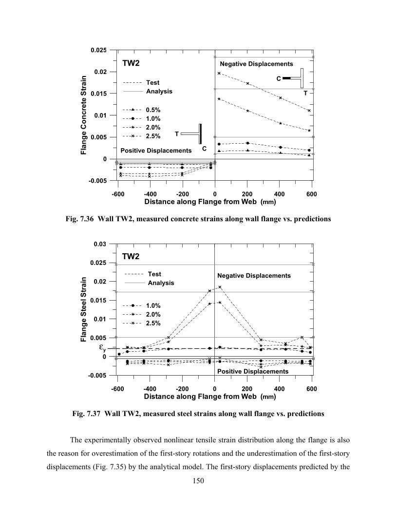
150
-600 -400 -200 0 200 400 600Distance along Flange from Web (mm)
-0.005
0
0.005
0.01
0.015
0.02
0.025
Flan
ge C
oncr
ete
Stra
in TestAnalysis
0.5%1.0%2.0%2.5%
TW2
Positive Displacements C
T
Negative Displacements
T
C
Fig. 7.36 Wall TW2, measured concrete strains along wall flange vs. predictions
-600 -400 -200 0 200 400 600Distance along Flange from Web (mm)
-0.005
0
0.005
0.01
0.015
0.02
0.025
0.03
Flan
ge S
teel
Stra
in
TestAnalysis
1.0%2.0%2.5%
TW2
Positive Displacements
Negative Displacements
εy
Fig. 7.37 Wall TW2, measured steel strains along wall flange vs. predictions
The experimentally observed nonlinear tensile strain distribution along the flange is also
the reason for overestimation of the first-story rotations and the underestimation of the first-story
displacements (Fig. 7.35) by the analytical model. The first-story displacements predicted by the

151
model are lower (despite overestimation of the inelastic rotations due to large tensile strains)
because the length of the plastic hinge region (the height over which steel yielding is observed) is
larger in the analytical model than that experienced by the wall specimen during testing.
The results presented in Figures 7.36–7.37 also reveal that the analytical model for the
wall specimen TW2 significantly underestimates the compressive strains in steel and concrete (as
was the case for RW2). Concrete and steel strains measured by the LVDTs and steel strain gages
along the length of the specimen web (including the web-flange intersection) are plotted for peak
top displacement points for selected lateral drift levels in Figures 7.38–7.39. The distribution of
tensile strains along the web is predicted with reasonable accuracy. It is interesting to observe
that the measured tensile strains in concrete (Fig. 7.38) tend to decrease suddenly at the web-
flange intersection due to the change in cross-section geometry.
0 200 400 600 800 1000 1200Distance along Web from Free End (mm)
-0.01
-0.005
0
0.005
0.01
Con
cret
e St
rain
Negative Displacements
-0.0050
0.0050.01
0.0150.02
0.0250.03
0.0350.04
Con
cret
e St
rain
0.5%1.0%1.5%
TestAnalysis
-0.0025
-0.00125
0
0.00125TW2
Positive Displacements
T
C
C
T
Fig. 7.38 Wall TW2, concrete strain measurements by LVDTs vs. predictions
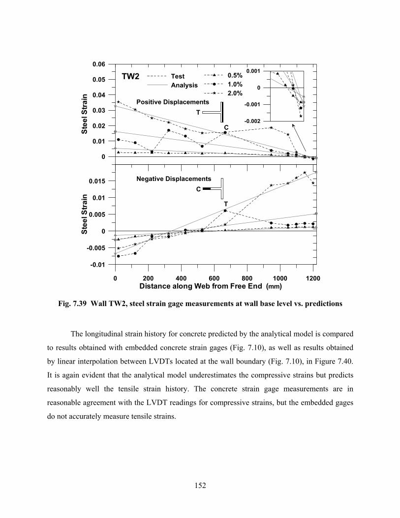
152
0 200 400 600 800 1000 1200Distance along Web from Free End (mm)
-0.01
-0.005
0
0.005
0.01
0.015
Stee
l Stra
in
Negative Displacements
0
0.01
0.02
0.03
0.04
0.05
0.06
Stee
l Stra
in0.5%1.0%2.0%
TestAnalysis
-0.002
-0.001
0
0.001TW2
Positive Displacements
C
T
T
C
Fig. 7.39 Wall TW2, steel strain gage measurements at wall base level vs. predictions
The longitudinal strain history for concrete predicted by the analytical model is compared
to results obtained with embedded concrete strain gages (Fig. 7.10), as well as results obtained
by linear interpolation between LVDTs located at the wall boundary (Fig. 7.10), in Figure 7.40.
It is again evident that the analytical model underestimates the compressive strains but predicts
reasonably well the tensile strain history. The concrete strain gage measurements are in
reasonable agreement with the LVDT readings for compressive strains, but the embedded gages
do not accurately measure tensile strains.
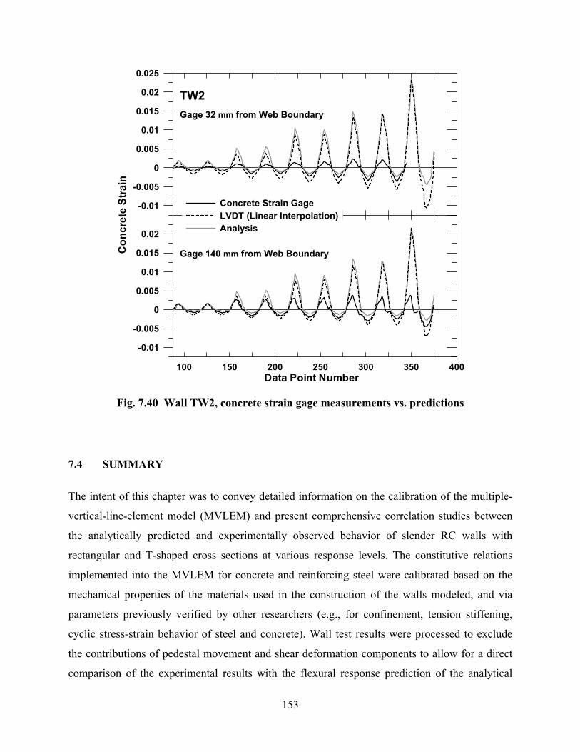
153
-0.01
-0.005
0
0.005
0.01
0.015
0.02
0.025
TW2
100 150 200 250 300 350 400Data Point Number
-0.01
-0.005
0
0.005
0.01
0.015
0.02
Con
cret
e St
rain
Concrete Strain GageLVDT (Linear Interpolation)Analysis
Gage 32 mm from Web Boundary
Gage 140 mm from Web Boundary
Fig. 7.40 Wall TW2, concrete strain gage measurements vs. predictions
7.4 SUMMARY
The intent of this chapter was to convey detailed information on the calibration of the multiple-
vertical-line-element model (MVLEM) and present comprehensive correlation studies between
the analytically predicted and experimentally observed behavior of slender RC walls with
rectangular and T-shaped cross sections at various response levels. The constitutive relations
implemented into the MVLEM for concrete and reinforcing steel were calibrated based on the
mechanical properties of the materials used in the construction of the walls modeled, and via
parameters previously verified by other researchers (e.g., for confinement, tension stiffening,
cyclic stress-strain behavior of steel and concrete). Wall test results were processed to exclude
the contributions of pedestal movement and shear deformation components to allow for a direct
comparison of the experimental results with the flexural response prediction of the analytical

154
model. The analytical model was subjected to the same conditions experienced during testing
(e.g., loading protocol, minor fluctuations in applied axial load). A refined configuration was
used for the model in order to predict the responses at specific locations where instrumentation
was provided for the tests. The correlation of the experimental and analytical results was
investigated in detail, at various response levels and locations (e.g., story displacements,
rotations over the first-story level, average strains in steel and concrete).
It was observed that the MVLE model, as implemented here, provides a good prediction
of the experimentally observed responses (wall lateral load capacity at varying drift levels, wall
displacement profile, average rotations and displacements over the region of inelastic
deformations) of the wall with rectangular cross section. The wall stiffness is well represented
both prior to, and after wall yielding, and the yield point is captured effectively. The model
provides a reasonably accurate prediction of wall tensile strains and the position of the neutral
axis, whereas the compressive strains tend to be underpredicted, possibly due to stress
concentrations at wall-pedestal interface or nonlinear shear deformations experienced within the
nonlinear flexural deformation region of the wall.
The same level of accuracy is observed in the prediction of the global response for T-
shaped walls when the flange is in compression, where the wall effectively behaves like a wall
with a rectangular cross section. When the flange is in tension, discrepancies between the results
obtained with the analytical model and the experimental results are observed for the wall lateral
load capacity and the displacements and rotations along the wall. Wall lateral load capacity and
inelastic rotations tend to be overestimated whereas inelastic lateral displacements are
underpredicted due to the observed nonlinear tensile strain distribution along the flange of the
wall, which cannot be captured by the MVLE model as implemented in this study.

8 Modeling of Coupled Shear and Flexural Responses: Analytical Model Description
As described in the previous chapter, the multiple-vertical-line-element model, as implemented
in this study, provides an accurate prediction of experimentally observed flexural wall response
at various response levels (wall load-displacement response, wall lateral load capacity at varying
drift levels, wall displacement profile, average rotations and displacements over the region of
inelastic deformations) for walls with rectangular cross sections. However, the model considers
uncoupled shear and flexural responses, and an improved modeling methodology is necessary for
simulating realistically the nonlinear shear responses associated with the interaction between
shear and flexural response components observed even in relatively slender RC walls (Massone
and Wallace, 2004).
Analytical models have been proposed to consider the observed coupling between
flexural and shear components of RC wall response. A recognized methodology involves
implementing the finite element method together with a constitutive RC membrane model that
follows a rotating-angle modeling approach (e.g., modified compression field theory, Vecchio
and Collins, 1986; rotating-angle softened-truss model, Pang and Hsu, 1995). A methodology
based on adopting this idea for a fiber model, was proposed by Petrangeli et al. (1999) to couple
shear response with flexural and axial responses. The analytical model proposed in this study is
based on applying the methodology developed by Petrangeli to the multiple-vertical-line-element
model. A description of the proposed modeling approach to incorporate coupling of wall flexural
and shear responses is presented in this chapter.
8.1 EXPERIMENTAL EVIDENCE OF FLEXURE-SHEAR INTERACTION
In order to demonstrate the observed coupling of flexural and shear responses in walls,
deformations associated with flexure and shear were investigated for two, well-instrumented,

156
approximately quarter-scale slender wall specimens with rectangular cross sections (specimen
RW2 tested by Thomsen and Wallace, 2004, and specimen SRCW1 tested by Sayre, 2003) to
assess their relative contributions to wall displacements. A summary of this experimental
investigation is provided in the following section; additional information is available in Massone
and Wallace (2004).
8.1.1 OVERVIEW OF TESTS
The two slender wall specimens used to assess the relative deformations associated with shear
and flexure were proportioned and detailed using capacity design and displacement-based design
approaches, respectively. The wall specimens were tested in an upright position. An axial load of
approximately 0.10Agf′c was applied to the wall specimens using hydraulic jacks mounted on top
of the load transfer assembly. The axial stress was held constant throughout the duration of each
test. Cyclic lateral displacements were applied to the walls by a hydraulic actuator mounted
horizontally to a reaction wall at 3.81 m above the base of specimen RW2 and to a reaction
frame at 4.88 m above the base of specimen SRCW1.
Specimen RW2 (also described in Chapter 7) was 3.66 m tall and 102 mm thick, with a
web length of 1.22 m. The longitudinal reinforcement at wall boundaries consisted of 8 – #3 (Ab
= 71 mm2) bars, whereas web reinforcement consisted of two curtains of deformed #2 (Ab = 32
mm2) bars placed horizontally and vertically, with a spacing of 189 mm on center. Specimen
SRCW1 was a structural steel reinforced concrete wall 4.88 m tall, 152 mm thick, and 1.22 m
long. Vertical reinforcement at wall boundaries consisted of a W6x9 section (Ab1 = 1729 mm2)
surrounded by 8 – #4 (Ab2 = 1032 mm2) bars. The web reinforcement consisted of two curtains
of horizontal and vertical #3 bars with a spacing of 152 mm on center. Design concrete
compressive strengths were 27.6 MPa for specimen RW2 and 34.5 MPa for specimen SRCW1.
Grade 60 (414 MPa) bars were used for longitudinal and web reinforcement of the specimens.
For SRCW1, A572, Grade 50 (345 MPa) W6x9 sections were used.
Instrumentation was used to measure displacements, loads, and strains at critical
locations for each wall specimen. Wire potentiometers (WPs) were mounted to a rigid steel
reference frame to measure lateral displacements along the height of the wall (Fig. 8.1). Linear
potentiometers (LPs) were mounted horizontally and vertically on the wall foundation to
measure any horizontal slip of the pedestal along the strong floor as well as rotations caused by

157
uplift of the pedestal from the strong floor. Measurements from the WPs used to record lateral
displacements were corrected to remove the contribution of pedestal slip and rotation to lateral
displacements.
Axial (vertical) displacements at the wall boundaries were measured using two WPs
mounted directly to the wall ends. These measurements were used to calculate wall story
rotations by dividing the difference in relative axial displacements by the distance between the
potentiometers. Shear deformations within the first two (RW2) and three (SRCW1) levels of the
wall specimens were determined using measurements from WPs placed diagonally on the walls,
in an “X” configuration (Fig. 8.1).
Linear variable differential transducers (LVDTs), oriented vertically over the wall length
just above the wall - pedestal interface, were used to obtained average axial strain and allow for
the determination of section curvature. The strains in the reinforcing steel also were measured
through the use of strain gages near the wall base and at other locations (Thomsen and Wallace,
2004; Sayre, 2003).
Wire Potentiometer(X configuration)
Wire Potentiometer(vertical displacement)
Wire Potentiometer(story lateral displacement)
Linear Potentiometer(pedestal displacement)
Linear Potentiometer(pedestal rotation)
Linear Potentiometer(pedestal rotation)
Fig. 8.1 General instrument configuration: RW2 and SRCW1

158
8.1.2 Instrumentation for Measuring Flexural and Shear Deformations
A common approach used to determine average (story) shear deformations for shear wall tests is
to use measurements from displacement gages placed diagonally in an “X” configuration (e.g.,
Thomsen and Wallace, 2004; see Fig. 8.2). However, as shown by Massone and Wallace (2004),
measurements obtained from the diagonal gages are influenced by flexural deformations if the
center of rotation of the story does not coincide with the geometric center of the story height. The
average shear deformations calculated using an “X” configuration may result in overestimation
of the shear deformations if not corrected to account for flexural deformations.
h D1
D2
Fig. 8.2 Uncorrected shear deformation measured at wall base
8.1.3 Measurement of Flexural Deformations
To determine the contribution of the flexural deformations to the lateral displacement at the top
of a story, the location of the centroid of curvature distribution (center of rotation) of the story
must be estimated. The flexural displacement at the top of the first story for a given curvature
distribution is calculated as:
Uf hα θ= (8.1)
where θ is rotation over story level, h is the story height, and α is the relative distance
from the top of the first story to the centroid of the curvature distribution. In this study, a value of
α = 0.67 was used, which is consistent with prior research (Thomsen and Wallace, 2004).
2_
222
221 hDhD
XoriginalUs−−−
=

159
8.1.4 Measurement of Shear Deformations: Corrected “X” Configuration
As proposed by Massone and Wallace (2004), the uncorrected story shear displacement
measured through the use of the “X” configuration of WPs and the story flexural displacement
measured using the vertical WPs at the wall boundaries can be used in combination to obtain a
“corrected” average story shear displacement (Us_Xcorrected) as:
1_ _2
Us Xcorrected Us Xoriginal hα θ⎛ ⎞= + − ⋅ ⋅⎜ ⎟⎝ ⎠
(8.2)
where Us_Xoriginal obtained using only the diagonal WP (X configuration)
measurements would give a biased estimation of the story shear displacement, due to
contribution of flexural deformations.
8.1.5 Experimental Force versus Displacement Relations for Shear and Flexure
Using the methodology described above to separate the contributions of shear and flexural
deformations in measured wall displacements, lateral load versus top and story deformation
relations can be determined. Figure 8.3 plots the applied story shear force versus measured
flexural (Fig. 8.3a) and shear (Fig. 8.3b) displacements within the first and second stories of
specimen RW2. Figure 8.4 plots the same relations for the first through third stories of specimen
SRCW1. Relations derived from the experimental data are compared to analytical results for
linear elastic analyses for a “fully cracked” section stiffness for flexure and an elastic shear
stiffness. The cracked section stiffness is obtained from a sectional analysis, as a secant stiffness
to the point of first yield of reinforcement. For simplicity, a linear elastic shear stiffness is
assumed.
Results for specimen RW2 are presented in Figure 8.3. At the second-story level of
specimen RW2, shear displacements were evaluated using only the diagonal potentiometer (X
configuration) measurements without correction given in Equation 8.2 because vertical
potentiometers were not provided during testing along the second-story height (Fig. 8.1). The
story shear force versus flexural displacement relations for specimen RW2 (Fig. 8.3a) reveal that
(1) the cracked stiffness obtained from a moment versus curvature analysis reasonably captures
the measured lateral stiffness of the wall prior to yield, (2) yielding of flexural reinforcement
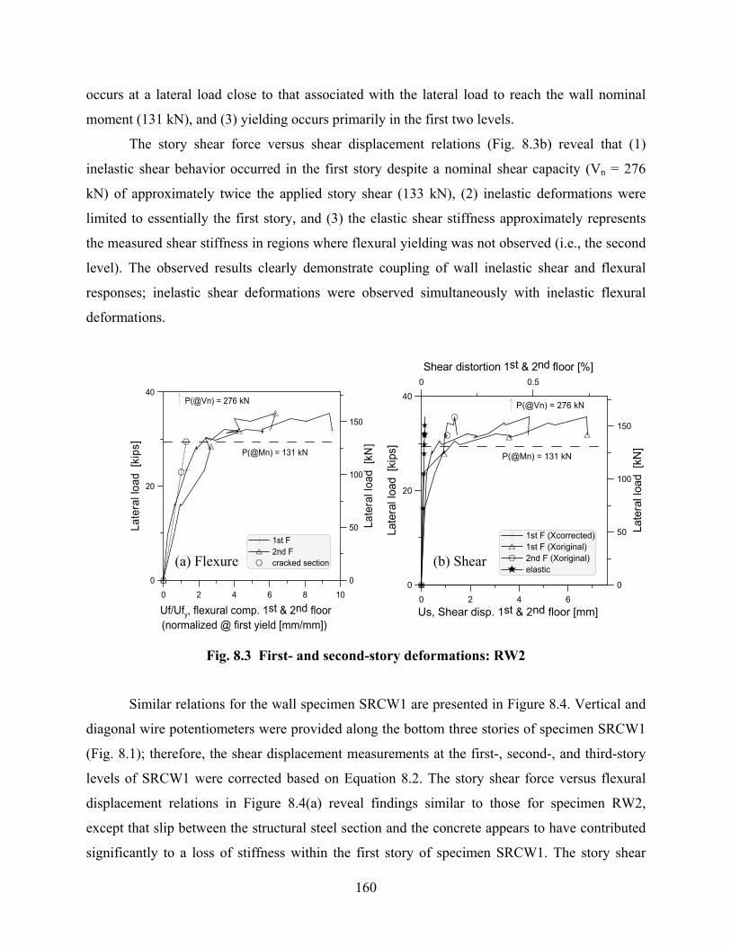
160
occurs at a lateral load close to that associated with the lateral load to reach the wall nominal
moment (131 kN), and (3) yielding occurs primarily in the first two levels.
The story shear force versus shear displacement relations (Fig. 8.3b) reveal that (1)
inelastic shear behavior occurred in the first story despite a nominal shear capacity (Vn = 276
kN) of approximately twice the applied story shear (133 kN), (2) inelastic deformations were
limited to essentially the first story, and (3) the elastic shear stiffness approximately represents
the measured shear stiffness in regions where flexural yielding was not observed (i.e., the second
level). The observed results clearly demonstrate coupling of wall inelastic shear and flexural
responses; inelastic shear deformations were observed simultaneously with inelastic flexural
deformations.
0 2 4 6 8 10
Uf/Ufy, flexural comp. 1st & 2nd floor(normalized @ first yield [mm/mm])
0
20
40
Late
ral l
oad
[kip
s]
1st F2nd Fcracked section
0
50
100
150
Late
ral l
oad
[kN
]
P(@Vn) = 276 kN
P(@Mn) = 131 kN
0
20
40La
tera
l loa
d [k
ips]
1st F (Xcorrected)1st F (Xoriginal)2nd F (Xoriginal)elastic
0
50
100
150
Late
ral l
oad
[kN
]
0 0.5Shear distortion 1st & 2nd floor [%]
0 2 4 6Us, Shear disp. 1st & 2nd floor [mm]
P(@Vn) = 276 kN
P(@Mn) = 131 kN
Fig. 8.3 First- and second-story deformations: RW2
Similar relations for the wall specimen SRCW1 are presented in Figure 8.4. Vertical and
diagonal wire potentiometers were provided along the bottom three stories of specimen SRCW1
(Fig. 8.1); therefore, the shear displacement measurements at the first-, second-, and third-story
levels of SRCW1 were corrected based on Equation 8.2. The story shear force versus flexural
displacement relations in Figure 8.4(a) reveal findings similar to those for specimen RW2,
except that slip between the structural steel section and the concrete appears to have contributed
significantly to a loss of stiffness within the first story of specimen SRCW1. The story shear
(a) Flexure (b) Shear

161
force versus shear displacement relations (Fig. 8.4b) reveal that inelastic shear behavior was
experienced within the first and second stories of the wall despite a nominal shear capacity (Vn =
651 kN) of approximately twice the applied story shear (310 kN). The observed inelastic shear
deformations in the first-story level, and also to a lesser degree in the second-story level, clearly
demonstrate the coupling of inelastic flexural and shear deformations. As well, the flexural and
shear force–deformation relations reach yielding at approximately the same time. This behavior,
which has also been observed in prior studies (e.g., Takayanagi et al., 1979), has been
established for the tests evaluated using an unbiased methodology for evaluating shear
deformations, and the results verified through the use of redundant measurements for multiple
test specimens (Massone and Wallace, 2004).
0 2 4 6 8 10Uf/Ufy, flexural comp. 1st, 2nd and 3rd floor
(normalized @ first yield [mm/mm])
0
20
40
60
80
Late
ral l
oad
[kip
s]
1st F2nd F3rd Fcracked section
0
100
200
300
Late
ral l
oad
[kN
]
P(@Vn) = 651 kN
P(@Mn) = 303 kN
0
20
40
60
80La
tera
l loa
d [k
ips]
1st F (Xcorrected)2nd F (Xcorrected)3rd F (Xcorrected)elastic
0
100
200
300
Late
ral l
oad
[kN
]
0 0.5Shear distortion 1st, 2nd & 3rd floor [%]
0 4 8
Us, Shear disp. 1st, 2nd & 3rd floor [mm]
P(@Vn) = 651 kN
P(@Mn) = 303 kN
Fig. 8.4 Story deformations: SRCW1
8.2 BASE MODEL: MULTIPLE-VERTICAL-LINE-ELEMENT MODEL (MVLEM)
The formulation of the multiple-vertical-line-element model (MVLEM) was extended to
simulate the observed coupling behavior between nonlinear flexural and shear responses in RC
walls. The MVLEM, as described in Chapter 3, resembles a two-dimensional fiber model,
simplified such that element rotations (curvatures) are concentrated at the center of rotation
defined for each element. In the MVLEM, a single average value of curvature is assumed for
(a) Flexure (b) Shear

162
each model element, as opposed to a generic displacement-based fiber model implementation
where a linear curvature distribution (displacement interpolation function) is used between
element nodes and the curvature distribution is integrated at Gaussian points to obtain element
rotations and displacements. A structural wall is modeled as a stack of MVLEs, which are placed
one upon the other, and the coupled axial-flexural response of each MVLE is simulated by a
series of uniaxial elements (or macro-fibers) connected to infinitely rigid beams at the top and
bottom (e.g., floor) levels (Fig. 8.5(a)) that enforce a plane section assumption. A horizontal
spring placed at the center of rotation (at relative height ch) of each MVLE, with a prescribed
nonlinear force-deformation behavior, is commonly used to simulate the shear response of the
element. Shear and flexural responses are considered uncoupled in the original formulation of the
MVLEM. The constitution and kinematics of the MVLEM are explained in detail in Chapter 3.
(a) MVLEM element (b) axial disp. (c) flexural disp. (d) shear disp.
Fig. 8.5 MVLEM element and incorporated displacement field components
8.3 INCORPORATING DISPLACEMENT INTERPOLATION FUNCTIONS
The original formulation of the multiple-vertical-line-element model was modified to
accommodate displacement interpolation functions and integration (Gaussian) points for
practical implementation of the model into computational platforms (e.g., OpenSees) in which
the displacement-based fiber model formulation is already built in. However, derivation of the
displacement interpolation functions implemented in the model incorporate the definition of an
element center of rotation in order to distinguish between model lateral displacements resulting
from shear and flexural deformations. The element center of rotation is defined at a fraction of
h (1-c)h
ch
wh
uh θh
y
w0
u0
θ0
u(y) wf (y)
γ (y)
+ + =

163
the element height ch, as in the case of the original MVLEM. Geometrically, the center of
rotation is defined as the point for which the transverse flexural displacement of the element
(Δwf, defined in Eq. 8.3), is equivalent to the displacement associated with the rigid body
displacement of the element, resulting from the rotation (Δθ, defined in Eq. 8.4) that the element
undergoes at the center of rotation. Accordingly, the center of the curvature (φ) distribution (or
the center of rotation) of the element is located at the relative element height ch, as shown in
Figure 8.6. 0
' ' ( )h h h
fo h o o
w x dx h x dx h dx xdxφ φ φ φΔ = = − − = −∫ ∫ ∫ ∫ (8.3)
h
o
dxθ φΔ = ∫ (8.4)
f fxdx h w wch h
dx
φ θθ θφ
Δ − Δ Δ= = = −
Δ Δ∫∫
=> (1 )fw h c θΔ = − Δ (8.5)
Fig. 8.6 Definition of center of rotation
In an attempt to locate the center of rotation for a slender cantilever wall, experimental
results from Sayre (2003) were investigated by Massone and Wallace (2004). Curvature
distributions measured by linear transducer (LVDT) pairs were used to evaluate the center of
rotation along the first-story level of a slender steel-reinforced concrete wall specimen.
Δθ
Δθ Δwf
Δwf
x’ x
h ch (1-c)h
x
Center of rotation (center of curvature)
ch (1-c)h
φ

164
Experimental data points were found to give an average center of rotation coefficient of c = 0.4
(Fig. 8.7) for the entire loading range, without significant scatter of the data when the wall is
subjected to nonlinear deformations. Therefore, a value of c = 0.4 is used in this study. Use of c
= 0.4 is also consistent with the studies by Vulcano et al. (1988) and Orakcal et al. (2004), who
recommended the same value for c, based on comparison of the analysis results using the
MVLEM with results of wall tests.
0 0.2 0.4 0.6 0.8 1
c factor
-400
-300
-200
-100
0
100
200
300
400La
tera
l loa
d [k
N]
φ > φy *φ < φy
* 4 measured curvatures
Fig. 8.7 Center of rotation for specimen SRCW3
The displacement interpolation functions implemented into the analytical model represent
the three displacement field components shown in Figure 8.5, which are associated with the axial
(u), flexural (wf), and shear (γ) deformations (or strains) of the element. Other than implementing
the idea of a center of rotation to segregate model transverse displacements into shear
deformation (integration of shear strain) and flexural deformation (double integration of
curvature distribution) components, the derivation of the displacement interpolation functions
considers a linear variation of axial deformations and curvatures, and a uniform distribution of
shear strain along the longitudinal axis (y) of the model element. Accordingly, the displacement
field of the two-node model element, with respect to the six degrees of freedoms illustrated in
Figure 8.5(a) is obtained as:

165
( )( )
( )
0
0
01 1
1 / 0 0 / 0 00 1 0 00 1/ 0 1/ 1
fh
h
h
uw
u y y h y hw y yc yc y
uy h c h c
w
θ
γ
θ
⎡ ⎤⎢ ⎥⎢ ⎥−⎡ ⎤ ⎡ ⎤⎢ ⎥⎢ ⎥ ⎢ ⎥= − + ⋅ ⎢ ⎥⎢ ⎥ ⎢ ⎥⎢ ⎥⎢ ⎥ ⎢ ⎥− − −⎣ ⎦⎣ ⎦ ⎢ ⎥⎢ ⎥⎢ ⎥⎣ ⎦
(8.6)
( ) ( ) 21 1 3 2 / 1 2 ( / )c c y h c y h= + − + − . (8.7)
This derivation considers that the rotation of the element longitudinal axis is described as
w′ = dw/dy = θ + γ (Fig. 8.8), where w represents the total lateral element displacement
(displacements due to flexure (wf) and shear), θ is the relative rotation of the cross-section
rotation, and γ is the uniform shear strain value (uniform along the element height and across
element cross section). As shown in Figure 8.8, when only the flexural deformation is
considered, the longitudinal axis of the element remains orthogonal to the element cross section,
and therefore the flexural lateral displacement (wf) is directly related to the rotation of the cross
section (θ) as dwf /dy = θ.
The displacement field is then rearranged, to be consistent with the finite element
formulation, in terms of axial displacement (u), total lateral displacement (w) and section rotation
(θ), yielding to:
( )( )( )
( )
0
0
03 3
4 4
1 / 0 0 / 0 00 1 / 0 /0 0 0 0 1
Nh
h
h
uw
u y y h y hw y y h yc y h yc N y U
uy c c
w
θ
θ
θ
⎡ ⎤⎢ ⎥⎢ ⎥−⎡ ⎤ ⎡ ⎤⎢ ⎥⎢ ⎥ ⎢ ⎥= − − ⋅ = ⋅⎢ ⎥⎢ ⎥ ⎢ ⎥⎢ ⎥⎢ ⎥ ⎢ ⎥−⎣ ⎦⎣ ⎦ ⎢ ⎥⎢ ⎥⎢ ⎥⎣ ⎦
(8.8)
( ) ( ) 23 1 3 2 / 1 2 ( / )c c c y h c y h= − + − + − (8.9)
( ) ( ) 24 1 2 3 2 / 3 1 2 ( / )c c y h c y h= + − + − (8.10)
where N(y) represents the element displacement interpolation functions for axial
displacement, transverse displacement, and rotation, and UN is the set of element nodal
displacements.
From the displacement field, the strain field is derived as:

166
( )( )( )
( )
0
0
02 2
1/ 0 0 1/ 0 00 0 2 / 0 0 2 /0 1/ 0 1/ 1
Nh
h
h
uduwdyy h h
dy c h c h B y Uudy
y h c h cw
εθθφ
γγ
θ
⎡ ⎤⎡ ⎤⎢ ⎥⎢ ⎥⎢ ⎥⎢ ⎥ −⎡ ⎤ ⎡ ⎤⎢ ⎥⎢ ⎥⎢ ⎥ ⎢ ⎥= = − ⋅ = ⋅⎢ ⎥⎢ ⎥⎢ ⎥ ⎢ ⎥⎢ ⎥⎢ ⎥⎢ ⎥ ⎢ ⎥− − −⎣ ⎦⎣ ⎦ ⎢ ⎥⎢ ⎥⎢ ⎥⎢ ⎥⎣ ⎦ ⎢ ⎥⎣ ⎦
(8.11)
( )2 2 3 3 1 2 /c c c y h= − + + − (8.12)
where B(y) represents the element strain interpolation functions for axial strain (ε),
curvature (φ), and shear strain (γ).
Incorporating these interpolation functions for displacement and strain converts the
kinematic formulation of the MVLE to a displacement-based fiber element, with special
interpolation functions adopted to incorporate shear deformations.
Fig. 8.8 Element section rotation
8.4 NONLINEAR ANALYSIS SOLUTION STRATEGY: FINITE ELEMENT FORMULATION
Similar to the original MVLE, the linearized equilibrium equation to conduct a quasi-static
analysis using the present model can be expressed in the form of Equation 8.13. For simplicity,
the following equations are expressed at the element level. A direct stiffness assembly, together
w’
y
Undeformed Deformed (flexure) Deformed (flexure + shear)
θ γ
w wf

167
with an iterative nonlinear analysis solution strategy (as described in Chapter 5), would be
required to perform a quasi-static analysis of an entire wall using the present element.
int 0dist nodalNK U f f f⋅ Δ + − − = (8.13)
The equilibrium equation represents the externally applied forces, in the form of
distributed or nodal forces. The distributed load (per unit length) vector is defined
as ( ) ( ) ( ) ( ) tP y p y q y m y= ⎡ ⎤⎣ ⎦ , where p(y) corresponds to the intensity of the distributed
axial load, q(y) represents the distributed transverse load, and m(y) is the distributed moment.
The distributed vector force (at the six element degrees of freedom shown in Figure 8.5(a)) can
be expressed as:
( ) ( ) ( ) ( )h
ttdist
o
f N y p y q y m y dy= ⋅⎡ ⎤⎣ ⎦∫ (8.14)
where N(y), as previously described, represents the displacement interpolation functions
for axial displacement, transverse displacement, and rotation.
The nodal forces are defined based on the magnitude of the axial forces, bending
moments and shear forces applied at the element degrees of freedom. The nodal-force vector is
thus expressed as:
[ ]0 0 0tnodal
h h hf N M V N M V= (8.15)
where axial forces (N), moments (M) and shear forces (V) are defined at both ends of the
element (ends denoted by subscripts 0 and h).
To attain equilibrium, the internal resisting force increments at the nodal degrees of
freedom of the model element must balance the externally applied force increments, for each
increment of nodal displacements applied on the element. The internal resisting forces at the
element degrees of freedom are determined by integrating the axial forces (N) and the shear
forces (V) resisted by each vertical sub-elements of the model element, as:
( ) ( ) ( ) ( )inth
tt
o
f B y N y M y V y dy= ⋅⎡ ⎤⎣ ⎦∫ (8.16)
( )th
t i i ii H
i i io
B y f f x f dy⎡ ⎤= ⋅⎢ ⎥⎣ ⎦∑ ∑ ∑∫
where B(y) represents the element strain interpolation functions for axial strain,
curvature, and shear strain, and fi is the axial force on each vertical sub-element, fiH is the shear

168
force on each vertical sub-element, and xi is the horizontal position of each vertical sub-element
relative to the longitudinal axis of the element.
The stiffness matrix K of the element, with respect to the displacements at the six element
degrees of freedom shown in Figure 8.5(a) is derived as:
( ) ( )h
t
o
K B y D B y dy= ⋅ ⋅∫ (8.17)
where D relates the internal forces on the element with element deformations (axial strain
ε, curvature φ, and shear strain γ), and is expressed as:
2
i i i
ii ii i iy y xy
i i i
i i ii ii i iy y xy
i i iH H H
ii ii i iy y xy
f f fN N N x
M M M f f fD x x x
V V V f f fx
ε ε γε φ γ
ε φ γ ε ε γ
ε φ γ ε ε γ
⎛ ⎞∂ ∂ ∂⎛ ⎞∂ ∂ ∂ ⎜ ⎟⎜ ⎟ ∂ ∂ ∂⎜ ⎟∂ ∂ ∂⎜ ⎟ ⎜ ⎟⎜ ⎟∂ ∂ ∂ ∂ ∂ ∂⎜ ⎟= =⎜ ⎟ ⎜ ⎟∂ ∂ ∂ ∂ ∂ ∂⎜ ⎟ ⎜ ⎟⎜ ⎟∂ ∂ ∂ ∂ ∂ ∂⎜ ⎟⎜ ⎟ ⎜ ⎟∂ ∂ ∂⎝ ⎠ ∂ ∂ ∂⎝ ⎠
∑ ∑ ∑
∑ ∑ ∑
∑ ∑ ∑
(8.18)
where y
iixε ε φ= + is the axial strain on each vertical sub-element and xi is the horizontal
position (distance from element longitudinal axis) of each vertical sub-element.
Finally the term ΔUN in Equation 8.15 is the incremental nodal-displacement vector and
is expressed as:
[ ]0 0 0t
N h h hU u w u wθ θΔ = Δ Δ Δ Δ Δ Δ (8.19)
8.5 MODELING OF SHEAR-FLEXURE INTERACTION
The analytical model proposed in this study, incorporates RC panel behavior in the multiple-
vertical-line-element-model (the original formulation of which considers uncoupled flexural and
shear responses) in order to capture the experimentally observed shear-flexure interaction in RC
walls (e.g., Massone and Wallace, 2004). The proposed wall model involves modifying the
MVLEM by assigning a shear spring for each uniaxial element. Each uniaxial element is then
treated as a RC panel element, with membrane actions, i.e., uniform normal and shear stresses
applied in the in-plane direction. Therefore, the interaction between flexure and shear is
incorporated at the uniaxial element (fiber) level. To represent constitutive panel behavior, a
rotating-angle modeling approach, as applied in the derivation of the modified compression field

169
theory (MCFT, Vecchio and Collins, 1986) or the rotating-angle softened-truss model (RA-STM,
Pang and Hsu, 1995), can be used. The constitutive rotating-angle modeling approach adopted in
this study follows the RA-STM; however, a more refined constitutive stress-strain model for
concrete in compression, which is calibrated with a large set of experimental results, is
implemented. Constitutive stress-strain models for materials are applied along the principal
directions of the strain field (i.e., principal strain directions 1 and 2), to obtain the stress field
associated with the principal directions. It is assumed that the principal stress and strain
directions coincide (as suggested by Vecchio and Collins, 1986; Pang and Hsu, 1995).
Accordingly, the axial and shear responses of each uniaxial (panel) element are coupled,
which further allows coupling of flexural and shear responses of the MVLEM, since the axial
response of the uniaxial elements constitute the overall flexural response of each MVLE. Details
of the methodology are described in the following subsection.
8.6 NUMERICAL METHODOLOGY FOR PROPOSED MODEL
In the following description of the methodology, the uniaxial (panel) elements located within
each model element (also called strips) are denoted by (i) and the model elements are denoted by
(j):
1. The deformations or strains within the components of each element (j) are determined
from the six prescribed degrees of freedom, (ux, uy, and θ at both ends of the model
element) shown in Figure 8.9. Assuming that the shear strain is uniform along the section
and that plane sections remain plane, the axial strain (εy), and shear distortion (γxy)
components of the strain field are calculated for the entire section (for all the strips (i))
based on the prescribed degrees of freedom for the current analysis step. Accordingly,
each strip (i) (Fig. 8.9) has two input variables, axial strain (εy) and shear distortion (γxy),
based on element (j) deformations. The horizontal (or transverse) normal strain within
each strip (εx) is initially estimated to complete the definition of the strain field, allowing
stresses and forces to be determined from the constitutive material relations and
geometric properties (dimensions and reinforcement and concrete areas) for each strip.
For the initial estimate of the horizontal strain within each strip (εx), a zero value or the
resulting value from the previous load step can be used. The output variables associated

170
with the input strains εy and γxy are the axial stress, σy, and the shear stress, τxy, for each
strip (i).
Strip (i)
εx - unknown ch
h
γxy - trial
εy - trial
N, Δuy
V, Δux
M, Δθ
Fig. 8.9 Trial displacement state at section (j) of coupled model element
2. A numerical procedure (Newton’s method) is employed to linearize the equilibrium
equation and iterate on the unknown quantity εx (horizontal normal strain in each strip i)
to achieve horizontal equilibrium for a given σx (resultant horizontal normal stress)
within each strip. The horizontal stress σx is the resultant of stress components in
concrete and steel that balances normal stress resulting from loads applied in the
horizontal direction. Due to a lack of information and as an initial approximation, the
horizontal stress σx within each strip was assumed to be equal to zero (no resultant
stress), which is consistent with the boundary conditions at the sides of a wall with no
transverse loads applied over its height. The horizontal strain, εx, is used as an iterative
parameter for convenience.
(a) For a trial value of horizontal strain (εx, together with the prescribed values of axial
strain (εy) and shear distortion (γxy)), the strain field (principal orientation angle α, and
the principal strains ε1 and ε2) is defined for each strip (i) (Fig. 8.10). It is assumed that
the same orientation angle (α) applies for the principal directions of both the strain (ε1,
ε2) and the stress fields (σc1, σc2). Using the constitutive material relations
implemented for concrete and steel (Fig. 8.11), and compatible strains for the two
materials (assuming perfect bond), the stresses in concrete along the principal
directions and stresses in reinforcement along the vertical and horizontal directions are

171
determined. As noted earlier, a uniaxial stress-strain model is used for the reinforcing
steel; therefore stresses in reinforcement are calculated in horizontal and vertical
directions (based on εx and εy, based on the assumption that reinforcement is provided
in the vertical and horizontal directions, or transformed to equivalent reinforcement in
the horizontal and vertical directions).
Fig. 8.10 Trial strain state at section (j) of coupled model element
Fig. 8.11 Trial stress state at strip (i) in section (j) in principal directions
(b) Stresses in concrete are transformed (Fig. 8.12) from the principal directions to the
reference coordinate directions (x-y) and the resulting concrete forces are
superimposed with the forces in the reinforcement based on the concrete and steel
areas within each strip (Fig. 8.13). The resultant gives average normal and shear
stresses in each strip (i) as:
( )1 2 sin 22
c cxy
σ στ α−= − ⋅ ⋅ (8.20)
( )1 2 1 2 cos 22 2
c c c cx cx x sx x sx
σ σ σ σσ σ ρ σ α ρ σ+ −= + ⋅ = − ⋅ ⋅ + ⋅ (8.21)
σC2 σC1
α Material Model concrete
ε2 ε1
α
σC
εC
ε2 ε1
α ε1 ε2 2α
(εy , γyx/2)
(εx , -γxy/2)
ε
γ/2 εy-trial
εx-unknown
γyx-trial
γxy
guess εx

172
( ) ( ) ( )1 2 1 2 cos 22 2
c c c cy cy y sy y sy
σ σ σ σσ σ ρ σ α ρ σ
+ −= + ⋅ = + ⋅ ⋅ + ⋅ (8.22)
Fig. 8.12 Trial stress state for concrete at strip (i) in section (j) in x-y direction.
Fig. 8.13 Trial stress state for concrete and steel (combined) in x-y direction
(c) Equilibrium is checked in the horizontal direction (σx) for each strip (i), until
equilibrium is achieved for the specified horizontal strain εx.
3. Once horizontal equilibrium is achieved for a specified tolerance within each strip,
vertical stresses in the strips are assembled to determine the total resisting axial force and
bending moment of each element, whereas the shear forces in the strips are assembled to
determine the total resisting shear force of the element.
4. Consequently, global equilibrium is checked for the overall wall model by comparing the
applied and resisting forces, and global iterations are performed on the model degrees of
freedom until global equilibrium is satisfied. Figure 8.14 shows a flowchart with the
internal numerical procedure.
σsy
σsx
σcx
τyx
τxy
σcy
+
Equilibrium resultant
σy=σcy+ρy*σsy
σx=σcx+ρx*σsx
τyx
τxy
σC2 σC1
α x-y coordinates concrete
σcy
σcx
τyx
τxy
σc1 σc2 2α
(σcy , τyx)
(σcx , -τxy)
σ
τ

173
Fig. 8.14 Flowchart for biaxial behavior
8.7 MATERIAL CONSTITUTIVE MODELS
As described in the previous section, the proposed modeling approach involves using two-
dimensional RC panel elements subjected to membrane actions, where the stiffness and force-
Variable set up
Convergence ?
NO YES
εx = εx + Δεx
σx_Trial = σcx + ρx* σsx
Compatibility
Material Laws
Equilibrium
Error = abs(σx_Trial- σx) < TOL σx = 0 (or other function)
+
+
τyxij = -(σc1 - σc2)*sin(2*α)/2
σyij = σcy + ρy* σsy
Global Trial Strains stage at strip (i) in section (j): εy γ
Global Trial Deformation stage at section (j): ux uy θ
(i) (j)
Global Equilibrium at trial deformation at section (j) (upper node)
Nj = Σ σyij * Aij
Vj = Σ τxyij * Aij
Mj = Σ σyij * Aij * xij - Vj*(1-
c)*h
Stresses at strip (i) in section (j)
Material prop.: fc’ εcr fcr Ec fy εsy … Reinforcement ratios: ρx ρy
Starting point (var.)
( )xyyx ,, γεεε1 ( )xyyx ,, γεεε 2 ( )xyyx ,, γεεα
Steel Concrete εx → σsx ε1, ε2 → σc1
σcx εy → σsy ε2, ε1 → σc2
σ

174
deformation properties of the panel elements are derived directly from material stress-strain
relations. Therefore, details of the constitutive relations used for reinforcing steel and concrete
are described in this section.
8.7.1 Constitutive Model for Reinforcing Steel
The stress-strain relation implemented in the wall model for reinforcing steel is the well-known
uniaxial constitutive model of Menegotto and Pinto (1973), as described in Chapter 4. The
relation is in the form of curved transitions (Fig. 8.21), each from a straight-line asymptote with
slope E0 (modulus of elasticity) to another asymptote with slope E1=bE0 where parameter b is
the strain-hardening ratio. The curvature of the transition curve between the two asymptotes is
governed by the parameter R (Fig. 8.21), the cyclic degradation of which permits the
Bauschinger effect to be represented. Cyclic properties of constitutive relation are not
incorporated in the present wall model; the model is yet to be extended for cyclic analysis.
However, the cyclic stress-strain response generated by the model is also illustrated in Figure
8.21 for further discussions.
To consider the effects of tension stiffening on reinforcement, Belarbi and Hsu (1994)
developed alternative average tensile stress-strain relations for steel bars embedded in concrete.
Belarbi and Hsu (1994) identified how the average stress-strain relation of reinforcing steel bars
surrounded by concrete is different than the stress-strain relation of bare steel bars. The most
important difference was found to be the lowering of the yield stress, σy, as yielding of a
reinforced concrete element occurs when the steel stress at the cracked section reaches the yield
strength of the bare bar. At the same time, the average steel stress smeared along the length of
the element reaches a level lower than that of the yield stress of the bare bar. The so-called
single-curve model can be directly incorporated in the Menegotto and Pinto equation, and has
been used for the calibration of the present wall model. As proposed by Belarbi and Hsu (1994),
and based on experimental data from the RC panels and an analytical model, the effective stress
and strain (intersection of the elastic and yield asymptotes) for bars embedded in concrete
correspond to approximately 91% of the yield stresses and strains of bare bars (σyeff = 0.91σy, εy
eff
= 0.91εy) and the monotonic curvature parameter R0 is described by the following empirical
relation:

175
01 25
9 0.2R
B= ≤
− (8.23)
1.51 cr
y
fBρ σ⎛ ⎞
= ⎜ ⎟⎜ ⎟⎝ ⎠
(8.24)
where fcr is the concrete cracking stress and ρ is the cross-sectional area ratio of the longitudinal
steel bars in the RC element (limited to a minimum of 0.25% in Mansour et al., 2001). The
monotonic curvature parameter R0 is limited to a value of 25, where the limiting value practically
represents a sharp corner between the elastic and yield asymptotes.
The so called “kinking effect” (reduction of effective yield stress due to dowel action
along the cracks) incorporated by Pang and Hsu (1995) in the original rotating-angle softened-
truss model is disregarded in this study based on later experimental observations by Hsu and Zhu
(2002), who stated that the kinking effect can be neglected.
For the case of cyclic loading, parameters rσ and rε represent the stress and strain at
each point of strain reversal, which together form the origin of elastic asymptote with slope 0E ,
and parameters 0σ and 0ε are the stress and strain at the point of intersection of the elastic and
yield. For monotonic loading, the cyclic stress and strain parameters retain the values 0=rσ ,
0=rε , effyσσ =0 , and eff
yεε =0 . Furthermore, for loading the curvature parameter R held
constant (R=R0), since there is no cyclic reduction (Bauschinger effect) in the curvature of the
stress-strain relation.
8.7.2 Constitutive Model for Concrete
To obtain a reliable model for panel (membrane) behavior, the constitutive relation implemented
in the analytical model for concrete should consider the effects of membrane (panel)
compression softening (reduction in principal compressive stresses in concrete due to cracking
under tensile strains in the orthogonal direction), and tension stiffening (average post-peak
tensile stresses in concrete due to the bonding of concrete and reinforcing steel between cracks).
Properties of the constitutive model adopted in this study for concrete are described in the
following subsections. For clarity, tensile and compressive stresses and strains are represented in
terms of absolute values.

176
Fig. 8.15 Constitutive model for reinforcing steel
To incorporate the tension-stiffening effect in the stress-strain behavior of concrete in
tension, the average (smeared) stress-strain relation proposed by Belarbi and Hsu (1994) (Fig.
8.22) is implemented, which is consistent with the selected constitutive material law for steel
based on average stresses and strains. To describe the stress-strain behavior of concrete in
compression, the Thorenfeldt base curve, calibrated by Collins and Porasz (1989), Wee et al.
(1996) and Carreira and Kuang-Han (1985), and updated via the introduction of the compression
softening parameter proposed by Vecchio and Collins (1993), is used. The envelope curve
selected allows for higher strain in low-strength concrete and a better correlation in the degrading
branch for high-strength concrete, where the envelope tends to be linear. The Thorenfeldt base
curve, which is based on the Popovics (1973) equation, takes the form (Fig. 8.23):
0'
0
1
c
c c nk
c
nf
n
εε
σεε
⎛ ⎞⎜ ⎟⎝ ⎠=⎛ ⎞
− + ⎜ ⎟⎝ ⎠
(8.25)
r
r
σσσσσ
−−=
0
*
r
r
εεεεε
−−=
0
*
( )
( ) RR
bb /1*
***
1
1
εεεσ
+
−+=
ξξ+
−=2
10 a
aRR
-0.01 -0.005 0 0.005 0.01 0.015 0.02
Strain, ε
-600
-400
-200
0
200
400
600
Stre
ss, σ
(M
Pa)
εyeff
E0
E1= bE0(εr
1,σr1)
(εr2,σr
2)(ε0
1,σ01)
(ε02,σ0
2) σyeff
1
1
ξ1*εyeff
ξ2*εyeff
R0
R(ξ1)
R(ξ2)
Monotonic Branch

177
where fc′ is the peak compressive stress (e.g., concrete compressive cylinder strength)
and ε0 is the strain at peak compressive stress for unconfined concrete in compression. For
defining of the strain at peak compressive stress (ε0 ), the expression proposed by Wee et al.
(1996) is used (Fig. 8.23). The following expressions proposed by Collins and Porasz (1989) are
used for the equation parameters n and k, for calibration of the model for relatively high-strength
concrete:
( )'
0.817
cf MPan = + (8.26)
( )0
'
0
1 , 0
0.67 , 62
ck f MPa
ε ε
ε ε
≤ ≤⎧⎪= ⎨
+ ≤⎪⎩
(8.27)
For concrete with lower compressive strengths (e.g., fc′ < 20 MPa), the following
expressions proposed by Carreira and Kuang-Han (1985) are considered for the same
parameters:
( ) 3'
1.5532.4
cf MPan
⎛ ⎞= + ⎜ ⎟
⎝ ⎠ (8.28)
1k = (8.29)
An important consideration in modeling the behavior of a RC panel element under
membrane actions is incorporating the compression softening effect. The softening effect has
been experimentally observed by many authors (e.g., Belarbi and Hsu, 1995; Vecchio and
Collins, 1986) mainly as a reduction in the compressive capacity of concrete panels along the
principal compressive direction undergoing tensile strains in the other principal direction. Some
models have also included softening in the compressive strain (e.g., Belarbi and Hsu, 1995;
Vecchio and Collins, 1993), reducing the strain at the peak compressive stress for concrete.
Vecchio and Collins (1993) used a large experimental database from tests on RC panels to
propose different models representing compression softening. In the tests, concrete strength (f′c)
for all specimens varied from 10 MPa to 90 MPa, where the main concentration of tests was in
the range 20–30 MPa. The concrete constitutive model was based on two main curves: the
Hognestad parabola and the Thorenfeldt curve. Both models were modified to include softening
in stress and strain. The so-called Model B, based on the Thorenfeldt curve, which considers
only a reduction in peak compressive stress ( cBModel
c βσσ = ), is implemented in this study, since

178
Vecchio and Collins (1993) observed that more complicated models (including also reduction in
the strain at peak stress, ε0) are only marginally better for incorporating the compression
softening effect. Accordingly, the reduction factor to be applied to the peak compressive stress
for concrete in compression (Fig. 8.23) is given by the expression:
1
0
1
0.9 0.27β ε
ε
=+
(8.30)
where ε1 is the principal tensile strain (Eq. 8.64 applies only when ε1 is a tensile strain)
and the ratio ε1 /ε0 is considered positive.
Fig. 8.16 Constitutive model for concrete in tension
The formulation of the analytical model presented in this chapter, together with the
material constitutive models used and the numerical solution methodologies described, has been
implemented into OpenSees (“OpenSees”) to conduct nonlinear analyses for evaluating the
validity and accuracy of the analytical model in simulating coupled shear and flexural responses
in RC walls. Experimental calibration of the model and comparison of model results with results
of tests conducted on both slender and squat wall specimens are presented in the following
chapter.
0 0.0005 0.001 0.0015 0.002 0.0025
Strain, εc
0
0.5
1
1.5
2
2.5
Stre
ss, σ
c (M
Pa)
(εcr ,fcr )
crc εε ≤ ccc E εσ =
crc εε > 4.0
⎟⎟⎠
⎞⎜⎜⎝
⎛=
c
crcrc f
εεσ
00008.0=crε
0.313 ( )cr cf f MPa′=
3917 ( )c cE f MPa′=
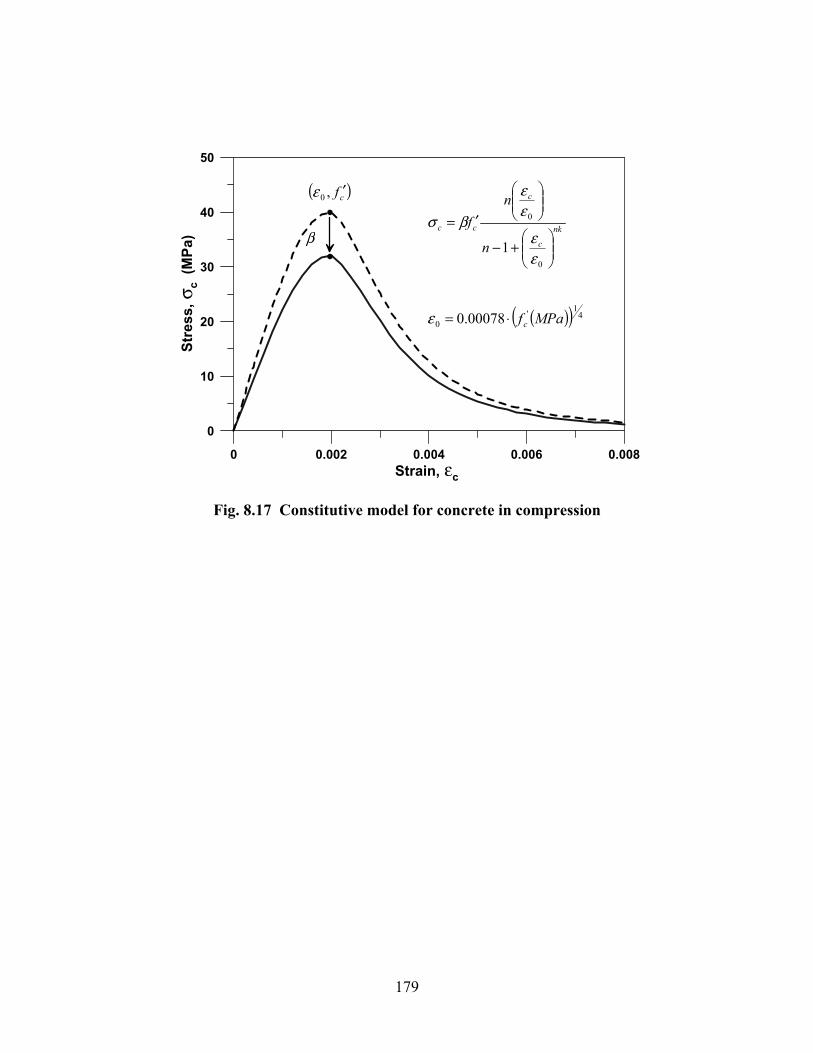
179
Fig. 8.17 Constitutive model for concrete in compression
nk
c
c
cc
n
nf
⎟⎟⎠
⎞⎜⎜⎝
⎛+−
⎟⎟⎠
⎞⎜⎜⎝
⎛
′=
0
0
1εε
εε
βσ
( )( ) 41'
0 00078.0 MPafc⋅=ε
0 0.002 0.004 0.006 0.008Strain, εc
0
10
20
30
40
50
Stre
ss, σ
c (M
Pa) β
( )cf ′,0ε

9 Modeling of Coupled Shear and Flexural Responses — Experimental Verification
The analytical model described in the previous chapter integrates material constitutive models
with a rotating-angle modeling approach to assemble a constitutive RC panel model. In modeling
of wall response, the analytical model incorporates further assumptions: the plane sections
remain plane kinematic, there is a uniform distribution of shear strains along the wall length, and
there is an assumed zero value for the resultant horizontal stress (σx) within each strip of the
model element. Due to the simplifications associated with the implemented membrane (panel)
material model (e.g., compression softening effect on stress only), idealizations of the rotating-
angle approach (e.g., principal strain and stress fields coincide assumption), and the assumptions
involved in the formulation of the present wall model (plane sections, uniform shear strains, zero
horizontal stresses), the validity of the model needs to be investigated for different wall
configurations. Therefore, this section presents information on the correlation of preliminary
model results with experimental results in order to evaluate the modeling approach. First, results
of the constitutive panel model are compared to experimental results from RC panel tests to
validate the response of model sub-elements. Then, the responses simulated by the wall model
are compared to test results on slender and short wall specimens. A discussion based on
experimental observations regarding the model assumptions (i.e., uniform shear strain
distribution along wall length and zero horizontal resultant stress across the wall) is also
provided.
9.1 PANEL BEHAVIOR
To verify the constitutive material models selected and the constitutive panel behavior
incorporated in the present wall model, results from tests conducted by prior researchers on RC
panel specimens subjected to pure shear loading conditions are compared to analytical responses

182
obtained using the constitutive panel model adopted. Two different sets of test series are used for
the comparisons (series A and B and series PV). Series A and B were tested by Pang and Hsu
(1995). The tested RC panel specimens were 1.4 m x 1.4 m x 178 mm thick, and were uniformly
reinforced with reinforcement area ratios varying between 0.6% and 3%. In-plane loads were
applied such that an equivalent pure shear loading condition (shear forces orthogonal/parallel to
the reinforcement) was achieved. Series PV was tested by Vecchio and Collins (1982). The
specimens had dimensions of 0.89 m x 0.89 m x 70 mm thick, and were uniformly reinforced
with reinforcing ratios varying between 0.7 and 1.8%. Pure shear loads were applied along the
sides of the specimens.
The constitutive panel element used in the present study was calibrated based on the
material properties and specimen geometry of selected test specimens, and subjected to a pure
shear loading condition to simulate the test conditions. Accordingly, comparisons of analytical
results with experimental results for the shear stress – shear strain response of the selected panels
are shown in Figure 9.1. As observed in the figure, a good correlation is obtained between the
element responses and test results, validating the selection of the constitutive material models
and the formulation of the panel elements incorporated in the present wall model. However, it
must be noted that the correlations presented are not for generalized loading conditions;
responses under only pure shear loading conditions are considered.
0.00 0.01 0.02 0.03Shear Strain
0
4
8
12
Shea
r Str
ess
(MPa
)
Specimens:A2A3A4B1B2
TestAnalysis
0.00 0.01 0.02 0.03
Shear Strain
0
1
2
3
4
5
Shea
r Str
ess
(MPa
)
Specimens:PV6PV11PV16PV19
TestAnalysis
Fig. 9.1 Test results vs. model element predictions for panel responses
(a) test series A and B
(b) test series PV

183
9.2 SLENDER WALL RESPONSE
Experimental observations indicate coupling between shear and flexural responses, even for
relatively slender walls (e.g., Massone and Wallace, 2004). Thus, correlation of preliminary
model results with results from a slender wall test is presented.
9.2.1 Test Overview
The rectangular wall specimen (specimen RW2 described in Chapter 8) tested by Thomsen and
Wallace (2004) was proportioned using a capacity design approach, and boundary element
details were based on using a displacement-based design methodology. Sufficient shear capacity
was provided for the wall specimen to resist the shear that developed for the probable wall
moment, using ACI 318-02 (Eq. 21.7). The wall specimen was 3.66 m tall and 102 mm thick,
with a web length of 1.22 m. The wall specimen was tested in an upright position, undergoing
top lateral cyclic displacements, while an axial load of approximately 0.07Agfc′ was held constant
throughout the duration of the test. More detailed information concerning the wall tests is
presented in Thomsen and Wallace (2004).
9.2.2 Model Calibration
To discretize the wall cross section for the analytical model, 16 strips (panel elements) were
defined along the length of the wall specimen, with corresponding tributary areas for concrete
and vertical reinforcement assigned to each strip. The horizontal reinforcement area was set
constant for all of the strips, which was consistent with the horizontal reinforcement used for the
specimen. A total of 8 model elements (each consisting of 16 strips) were stacked along the
height of the wall. The constitutive relations implemented in the model for reinforcing steel and
concrete were calibrated to represent the experimentally observed properties of the materials
used in the experimental study (using results of monotonic stress-strain tests conducted on
concrete and rebar specimens). Confinement and tension-stiffening effects were incorporated in
modeling (e.g., Orakcal and Wallace, 2004).

184
9.2.3 Model Correlation with Test Results
Prior to analysis, the experimental results for wall lateral displacements at story levels were
separated into flexural and shear response components using the methodologies described by
Massone and Wallace (2004) (see also Chapter 8) to allow comparison of model results to local
(e.g., story) shear and flexural response measurements. Results of monotonic analysis with the
proposed model were compared with the cyclic test results for the slender wall specimen.
Figure 9.2 compares the analytical and experimental lateral load – top displacement
responses for the wall specimen. As observed in Figure 9.2, the lateral load capacity and the
lateral stiffness of the wall are significantly overestimated for lower lateral drift levels (i.e., up to
0.75% drift) and overestimated to a lesser extent for higher lateral drift levels. The
overestimation of the wall capacity and stiffness, especially at lower drifts, can be attributed to
the fact that analysis results for monotonic loading are compared to cyclic test results. The
cyclic degradation of the curvature parameter R (Fig. 8.21) associated with the implemented
constitutive model for reinforcing steel influences significantly the wall lateral load capacity and
stiffness prediction, especially within the pre-yield and relatively low post-yield drift levels
(Orakcal et al., 2004). The present monotonic constitutive model for reinforcement does not
consider the cyclic degradation of the parameter R, impairing the response prediction. It must be
noted that results presented are preliminary, and additional studies to incorporate cyclic behavior
and to improve the material relations for a more refined calibration are under way.

185
-100 -80 -60 -40 -20 0 20 40 60 80 100Top Displacement, Δtop (mm)
-200
-150
-100
-50
0
50
100
150
200
Late
ral L
oad,
Pla
t (k
N)
TestAnalysis
≈Pax 0.07Ag f c'
Plat , Δtop
RW2
Fig. 9.2 Lateral load – top displacement response of specimen RW2
Figure 9.3 presents the correlation of analytical and experimental results for the lateral
load – flexural displacement and lateral load – shear displacement responses at the first-story
level of specimen RW2. The figure reveals that the model overestimates the flexural
deformations and underestimates the shear deformations measured within the first story of the
wall specimen. Again, the correlations would be significantly improved upon incorporating
cyclic analysis. However, as observed in the figures, the model is capable of capturing the
nonlinear shear deformations experienced simultaneously with the nonlinear flexural
deformations within the first story of the wall specimen, and thus successfully incorporates
coupling of nonlinear shear and flexural responses that were observed experimentally even for a
relatively slender wall.

186
-20 -15 -10 -5 0 5 10 15 20Lateral Flexural Displacement (mm)
-200
-150
-100
-50
0
50
100
150
200La
tera
l Loa
d (k
N)
TestAnalysis
-6 -4 -2 0 2 4 6
Lateral Shear Displacement (mm)
TestAnalysis
Fig. 9.3 Lateral load–displacement responses at first-story level (RW2)
9.3 SHORT WALL RESPONSE
As mentioned earlier, the proposed methodology to couple shear and flexural responses involves
three main assumptions: shear strains are uniformly distributed across the wall cross section, the
resultant horizontal stresses along the length of the wall are zero, and plane sections remain
plane. In the case of tall walls, the first assumption (i.e., uniform distribution of shear strain) may
not influence significantly the overall wall response, since the governing response component is
flexure. However, for short walls, using the same assumption may not be reasonable due to
possible presence of different modes of deformation (e.g., warping) or different load transfer
mechanisms (e.g., strut action), or other possible reasons such as the so-called Saint-Venant’s
effect, where the relatively small height of the wall may not be adequate to allow redistribution
of stresses concentrated within the proximity of the points of load application or where support
reactions are present. Such effects introduce nonuniformity in stresses and strains that may
change considerably the observed wall response. A similar condition applies to the zero
horizontal stress and plane section assumptions.
Thus, correlation of model results with test results on short wall specimens is presented to
assess the validity of the modeling approach for short walls. A more detailed calibration and
correlation study is under way; only general comparisons with limited experimental data are

187
included here. Test results available in the literature for four specimens with low shear-span
ratios are used for the comparisons.
9.3.1 Overview of Tests
Two wall specimens tested by Hidalgo et al. (2002) (specimens 10 and 16), and two specimens
reported by Hirosawa (1975) (specimens 74 and 152) are investigated here. These four wall tests
were selected because they represent a variety of wall configurations, specimen sizes, and
loading conditions. For each of the four selected test specimens, the amount of shear
reinforcement provided was no less than the minimum specified in the ACI 318-02 (2002), i.e.,
ρmin=0.0025. General specimen information for the four wall tests is shown in Table 9.1. As
shown in the table, all specimens had shear-span ratios (M/(Vl)) between 0.35–1.0. Specimens
10, 16, and 152 were designed to fail in shear. In those cases, the shear capacity was about half
the capacity to reach flexural failure. Specimen 74, in the other hand, was reported to fail in
flexure, but primarily deformed in shear. However, according to ACI 318-02, flexural and shear
capacities are similar (Fig. 9.4(a)).
Specimens 10 and 16 had similar reinforcement configurations; the shear-span ratio was
the main varying parameter between the two specimens (0.69 and 0.35 for specimens 10 and 16,
respectively). Relatively low shear-span ratios were achieved in the testing of these specimens
via fixing the base of the walls and avoiding rotations at the top of the walls by applying the
lateral load at specimen midheight, which produces a linear bending moment distribution with
moments equal in magnitude and opposite in direction applied at the wall ends. Both specimens
were designed to fail in shear by providing a relatively large amount of longitudinal
reinforcement at wall boundaries. Specimen 74 is the only specimen subjected to axial load and
is also the specimen with the largest shear-span ratio (M/(Vl)=1.0). It was tested under a
cantilever loading condition, with lateral load applied at the top of the wall. Another distinct
property of the specimen is that the shear and flexural capacities (according to ACI 318-02) of
the specimen are close, the shear capacity being slightly lower. Finally, specimen 152, having a
barbell-shaped cross section, was tested as a short beam with a concentrated transverse load
applied at midspan. From symmetry, half of the specimen represents a short wall where half of
the applied transverse load corresponds to an equivalent lateral load applied to the wall, yielding
a shear-span ratio of 0.56.

188
Table 9.1 Properties of selected short wall specimens
Reported by Hidalgo et al. (2002) Hirosawa (1975) Test no 10 16 74 152
lw clear length (cm) 130 170 170 208 hw total height (cm) 180 120 170 152 tw web thickness (cm) 8 8 16 16 lb boundary length (cm) - - - 32 tb boundary thickness (cm) - - - 32 M/(Vl) shear-span ratio - 0.69 0.35 1.00 0.56 ρh web horizontal steel ratio (%) 0.25 0.25 0.57 0.62 ρv web vertical steel ratio (%) 0.25 0.25 0.61 0.58 Ab boundary vertical steel (cm2) 7.6 6 15.5 66.4 N axial load (kN) 0 0 533 0
9.3.2 Model Calibration
The analytical model was calibrated to represent the geometric properties of the wall specimens,
using 8 model elements stacked along the height of each wall, where each element model
consisted of 8 strips (panel elements) defined along the length of the wall. Two strips were
defined for each boundary element of the specimens, whereas the remaining 4 were used to
discretize the web. Similar to the case for the slender wall, a more refined discretization of the
model did not change considerably the analytical responses obtained for the short walls; this
issue is addressed in a subsequent section. Corresponding tributary areas for concrete and
vertical reinforcement were assigned to each strip, whereas a constant horizontal reinforcement
area was used for each strip. Similar to the case for the slender wall test, the constitutive material
parameters were calibrated based on available experimental data reported on the mechanical
properties of the materials used in the construction of the wall specimens.
9.3.3 Model Correlation with Test Results
Figure 9.4 shows the correlation of experimental and analytical results for the lateral load –
displacement response of each of the four wall specimens. Analytical results were not obtained
for large lateral displacement values within the post-peak (degrading) branch of analytical
response, since the results in that range are subject to the so-called damage localization problem
(i.e., analysis results for the degrading response are sensitive to the discretization of the model
elements). Thus, degrading responses are not considered in the present study.

189
As observed in Figure 9.4(a), a very good correlation is obtained between test results and
results of the proposed coupled shear-flexure model for specimen 74 (M/(Vl)=1.0). Since the
design flexural and shear capacities of the specimen are close, to consider the possibility that the
response of the specimen is governed by nonlinear flexural deformations (i.e., the specimen does
not experience significant nonlinear shear deformations), Figure 9.4(a) also includes an
analytical flexural response prediction (with shear deformations not considered) obtained using a
fiber model. The same geometric discretization and material constitutive models used in the
coupled model were adopted for the fiber model, with the distinction that the panel elements
(strips) of the coupled model were replaced with uniaxial (fiber) elements, and the constitutive
model used for concrete in compression did not incorporate the biaxial compression softening
factor coefficient (β ). Figure 9.4(a) illustrates that although the flexural (fiber) model provides a
ballpark estimation of the wall lateral load capacity, (predicted lateral load capacities
approximately 750 kN and 980 kN, respectively for the coupled and flexural models), the load-
displacement response obtained by the flexural model is significantly different than the measured
response and the coupled model response. After a lateral load of 450 kN, significant lateral
stiffness degradation is observed in both the test results and results of the coupled model but not
in the flexural model. This result demonstrates how the proposed model, which couples shear
and flexural responses, is able to simulate observed responses with substantially greater accuracy
than a flexural model, particularly for wall specimens where the nominal shear and flexural
capacities are nearly equal.

190
0 0.2 0.4 0.6 0.8
Lateral Displacement (cm)
0
100
200
300
400
Late
ral L
oad
(kN
)
TestAnalysis(c) specimen 152 (d) specimen 16
0 0.4 0.8 1.2 1.6Lateral Displacement (cm)
0
500
1000
1500
2000
2500
Late
ral L
oad
(kN
)
TestAnalysis
0 0.4 0.8 1.2 1.6Lateral Displacement (cm)
0
50
100
150
200
Late
ral L
oad
(kN
)
TestAnalysis (b) specimen 10 (a) specimen 74
0 0.4 0.8 1.2 1.6 2Lateral Displacement (cm)
0
400
800
1200
Late
ral L
oad
(kN
)
Flexural AnalysisTestAnalysis
Fig. 9.4 Lateral load–displacement responses for short wall specimens
The correlation between results of the coupled model and test results for specimen 10
(M/(Vl)=0.69) is similar to that of specimen 74 (Fig. 9.4b). The model provides a good
prediction of the lateral load capacity and lateral stiffness of the wall specimen for most of the
top displacement history, although the wall specimen reaches its peak lateral load capacity at a
smaller top displacement than that predicted by the model. The sudden lateral load reductions
observed in the model response are due to sequential cracking of concrete, whereas such
behavior is not observed in test results. Refining the model discretization (increasing the number
of strips used along the length of the wall) would invoke a more gradual and continuous shape
for the analytical load-displacement response.

191
A relatively poor correlation is obtained between model and test results for the peak
lateral load capacity of specimen 152 (M/(Vl)=0.56), for which the model underestimates the
peak lateral load capacity of the specimen by approximately 25% of the measured value (Fig.
9.4c). However, the analytical model provides a good prediction of the wall lateral stiffness at
lower lateral load levels, and the general shape of the nonlinear response simulated by the model
is reasonable.
However, the correlation for specimen 16 (M/(Vl)=0.35) is far from being reasonable,
where the analytical model underpredicts the measured lateral load capacity of the wall by up to
50% for the entire loading history (Fig. 9.4d). Specimen 16 was subjected to the same loading
conditions as specimen 10 (M/(Vl)=0.69) and also had a similar reinforcement configuration; the
shear-span ratio was the main differentiating parameter between the two specimens. Thus the
difference between the accuracy in the predictions presented in Figures 9.4(b) and (d) is
associated directly with variation in shear-span ratios of the two specimens.
Overall, the correlations indicate that the accuracy of the proposed model in predicting
wall response is progressively impaired as the shear-span ratio of the wall modeled is reduced.
The best correlation is obtained for specimen 74 (M/(Vl)=1.0), whereas results for specimen 16
(M/(Vl)=0.69) were generally good. Results for specimen 152 (M/(Vl)=0.56) showed a relatively
poor but reasonable correlation, and the model was not successful in predicting the response of
specimen 16 (M/(Vl)=0.35). Therefore, it is apparent that the validity of the modeling approach
and the model assumptions are violated as wall shear-span ratios decrease. In a wall with a small
shear-span ratio, stresses and strains can follow significantly nonlinear distributions as opposed
to the assumptions incorporated in the present model (uniform shear strain distribution and zero
horizontal stress along wall length).
9.4 SENSITIVITY OF SHORT WALL ANALYTICAL RESULTS TO MODEL DISCRETIZATION
A parametric study was conducted to investigate the sensitivity of the analytical results to the
number of model elements stacked along wall height and the number of strips defined along wall
length. The pre-peak region of the analytical load-displacement response was found to be
insensitive to the selection of either the number of elements or the number of strips provided that
reasonable values are selected in order to adequately represent the overall wall geometry. Figure
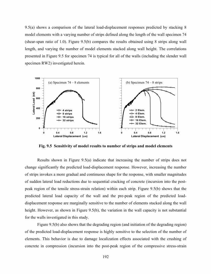
192
9.5(a) shows a comparison of the lateral load-displacement responses predicted by stacking 8
model elements with a varying number of strips defined along the length of the wall specimen 74
(shear-span ratio of 1.0). Figure 9.5(b) compares the results obtained using 8 strips along wall
length, and varying the number of model elements stacked along wall height. The correlations
presented in Figure 9.5 for specimen 74 is typical for all of the walls (including the slender wall
specimen RW2) investigated herein.
0 0.4 0.8 1.2 1.6Lateral Displacement (cm)
0
200
400
600
800
1000
Late
ral L
oad
(kN
)
4 strips8 strips16 strips32 strips
0 0.4 0.8 1.2 1.6
Lateral Displacement (cm)
2 Elem.4 Elem.8 Elem.16 Elem.32 Elem.
(a) Specimen 74 – 8 elements (b) Specimen 74 – 8 strips
Fig. 9.5 Sensitivity of model results to number of strips and model elements
Results shown in Figure 9.5(a) indicate that increasing the number of strips does not
change significantly the predicted load-displacement response. However, increasing the number
of strips invokes a more gradual and continuous shape for the response, with smaller magnitudes
of sudden lateral load reductions due to sequential cracking of concrete (incursion into the post-
peak region of the tensile stress-strain relation) within each strip. Figure 9.5(b) shows that the
predicted lateral load capacity of the wall and the pre-peak region of the predicted load-
displacement response are marginally sensitive to the number of elements stacked along the wall
height. However, as shown in Figure 9.5(b), the variation in the wall capacity is not substantial
for the walls investigated in this study.
Figure 9.5(b) also shows that the degrading region (and initiation of the degrading region)
of the predicted load-displacement response is highly sensitive to the selection of the number of
elements. This behavior is due to damage localization effects associated with the crushing of
concrete in compression (incursion into the post-peak region of the compressive stress-strain

193
relation). For the walls investigated, wall lateral load capacity is governed by the compressive
strength of concrete (i.e., the failure mode is concrete crushing). Thus, the post-peak region of
the stress-strain behavior of concrete in compression controls the degrading region of the
analytical load-displacement response. The present model cannot reliably predict this strength
degradation, without implementation of a proper damage localization parameter to calibrate the
post-peak (descending) region of the compressive stress-strain behavior of concrete based on the
size (height) of the elements used. This study focuses on predicting the pre-peak load-
displacement response and the lateral load capacity of walls; modeling of damage localization
and predicting degrading responses is not addressed.
9.5 EXPERIMENTAL SHEAR STRAIN AND HORIZONTAL NORMAL STRAIN DISTRIBUTIONS IN SHORT WALLS
As a supporting discussion on the potential of improving the model assumptions for a better
representation of short wall response, measured shear and horizontal strain distributions as part
of an experimental program are presented. Results of two wall tests conducted by Maier and
Thurlimann (1985) were investigated.
Two identical wall specimens (specimens S1 and S2), with shear-span ratios of 1.0 and
barbell-shaped cross sections with large boundary zones were loaded monotonically under a
cantilever loading condition with lateral loads applied at the top of the walls. The specimens
were 1.2 m height, 1.18 m long (boundary elements included) and 0.1 m thick. The boundary
elements were 0.4 m long and 0.1 m thick. Uniform steel web reinforcement was included in
vertical and horizontal directions. The steel reinforcement ratio in both directions was 1%. The
boundaries were reinforced with longitudinal rebars in a ratio of 1.26% of the boundary area.
The compressive concrete capacity was 36.9 MPa and the yield stress of the reinforcement 574
MPa. Both specimens were loaded with a constant axial load. Specimen S1 had an axial load of
about 0.07f′cAg, whereas specimen S2 had a higher axial load of about 0.25Agf′c (where Ag
corresponds to the total cross-section area).

194
9.5.1 Shear Strain Distributions
Vertical and horizontal displacements were measured at 63 points that constitute a mesh on the
web of the specimen (Fig. 9.6a), and shear strains were calculated from the displacement
measurements at each point on the mesh. Results obtained for the two specimens were similar in
terms of shear strain distributions; thus, results for only specimen S2 are presented here.
12......9
a b
0
1
2
3
4
5
6
7
8
9
10
Load Case 37
a b
Shear Strain 0.00333Level Distance 141mm
0
1
2
3
4
5
6
7
8
9
10
Load Case 70
a b
Shear Strain 0.01666Level Distance 141mm a b
γ γ
a b Plat (930 kN max.)
a b
Plat = 680 kN γ = 0.0033
Plat = 920 kN γ = 0.0167
(b) shear strains atwall first yield
(c) shear strains at wall capacity
(a) test setup and instrumentation
Fig. 9.6 Shear strain measurements for specimen S2
For two different lateral load levels (corresponding to yielding of the wall and at
maximum wall capacity), the distribution of shear strains along the horizontal direction at
different vertical levels of the wall specimen are plotted in Figure 9.6(b)–(c). The shear strains at
each vertical level are plotted using a continuous line along the horizontal direction, and the
horizontal dotted lines represent a zero shear strain line for reference. The figure reveals a
systematic nonlinear shear strain distribution, at both lateral load levels. The shear strains are
distributed in the horizontal direction at different vertical wall levels such that the position of the
maximum shear strain experienced at each vertical level approximately follows a diagonal line
traced between the point of the applied load and the lower opposite corner (compression strut).
This contradicts the model assumption that shear strains are distributed uniformly along the
length of the wall, as observed here for a wall with a shear-span ratio of 1.0. Comparison of

195
experimental and model results for specimen 74 (see previous section), which also has a shear-
span ratio of 1.0, is very good; therefore, the model assumption works well in this case.
However, the nonlinear distribution of shear strains may be more pronounced for shorter walls,
which may modify the responses of wall specimens with smaller shear-span ratios (e.g.,
specimen 16).
9.5.2 Horizontal Normal Strain Distributions
As complementary to the previous discussion related to experimental versus assumed shear strain
distribution, another discrepancy and potential improvement of the model assumptions of short
wall response is presented. In this case, measured horizontal strain distributions as part of the
experimental program by Maier and Thurlimann (1985) are presented. The results only for
specimen S2 are included here.
The same two different lateral load levels (corresponding to yielding of the wall and at
maximum wall capacity) used for the shear strain distributions in the previous discussion were
used in this analysis. The distribution of horizontal strains along the horizontal direction at
different vertical levels of the wall specimen is plotted in Figure 9.7(b)–(c). As was the case for
shear strains, the peak values of the horizontal normal strain measurements follow compression
strut. Furthermore, on average, the horizontal strain measurements decrease. In both load cases
(Fig. 9.7(b)–(c)), the horizontal strain at levels 1 (bottom) and 9 (top) are relatively small
compared to all other levels, and the strains tend to increase closer to wall midheight. Although
this affect is also apparent in the measured shear strain distributions, it is much more pronounced
for horizontal strains. The effect is clearly observed in Figure 9.8, which plots average horizontal
strain (average over the cross section) measurements along wall height.
Figure 9.8 shows the average horizontal normal strains measured at different levels along
the height of the wall for three different applied load levels (P = 920kN at wall capacity, P =
680kN at wall first yield and P = 810kN as an intermediate case). Analytical (model) results are
also included in the figure; however, analysis results are only available for the first two load
levels, as the analytical model predicted the wall to fail before it reaches a load of 810 kN. As
observed in the experimental results, the horizontal strain measurements have maximum values
at wall midheight, and progressively decrease to zero values at the top and the bottom of the
wall. In contrast, the analytical model, which assumes zero-resultant horizontal stress at every

196
location on the wall, predicts the horizontal strains to be increasing from the top (where lateral
load is applied) to the bottom of the wall. This implies that the analytical model overestimates
the horizontal strains in the vicinity of the top and bottom ends of the wall.
The experimental distribution of the horizontal normal strains along the height of the wall
is partially due to the so-called constraining effect of beam and pedestal located at the top and
bottom of the wall, and has been observed also by other researchers (e.g., Hsu, 1988; Cheng et
al., 1993). The significance of considering this effect in the modeling methodology is described
in the following section.
0
1
2
3
4
5
6
7
8
9
10
Load Case 70
a b
Shear Strain 0.00666Level Distance 141mm
0
1
2
3
4
5
6
7
8
9
10
Load Case 37
a b
Shear Strain 0.00167Level Distance 141mm
12......9
a b a b
εx εx
a b Plat
(930 kN max.)
a b Plat = 680 kN εx = 0.0017
Plat = 920 kN εx = 0.0067
(b) horizontal strains at wall first yield
(c) horizontal strains at wall capacity
(a) test setup and instrumentation
Fig. 9.7 Horizontal strain (εx) measurements for specimen S2
0 0.0005 0.001 0.0015 0.002 0.0025εx average
0
1
2
3
4
5
6
7
8
9
10
P=920kNP=810kNP=680kN
testmodel
Fig. 9.8 Average horizontal strain (εx) measurements for specimen S2

197
9.6 SENSITIVITY OF SHORT WALL ANALYTICAL RESULTS TO THE ZERO-RESULTANT-HORIZONTAL-STRESS ASSUMPTION
As discussed in a previous section, the validity of the modeling approach and the model
assumptions are violated as wall shear-span ratios decrease. In walls with relatively small shear-
span ratios (e.g., specimens 152 and 16), the distribution of stresses and strains can be
significantly different than the assumptions incorporated in the present model (uniform shear
strain distribution along wall length and zero-resultant horizontal stress along wall length and
height), impairing the correlation between model predictions and test results.
As part of ongoing studies to improve the formulation of the model for a better prediction
of the response of walls with low shear-span ratios, the sensitivity of the model results to
variations in the zero-resultant-horizontal-stress assumption was investigated. Prior studies by
Cheng et al. (1993) revealed that, for walls with low aspect ratios (e.g., h/l = 0.5), the horizontal
strains developed along the length of the wall are significantly reduced, especially in regions
close to the top and bottom of the wall, partially due to the constraining effect of the pedestal (or
beam) at the bottom and the beam at the top of the wall. Thus, for modeling, using an assumption
of zero horizontal normal strain (εx = 0), especially in regions close to the top and bottom of the
wall, may be more appropriate than assuming zero-resultant horizontal stress (σx = 0) along the
entire height of a wall with a low shear-span ratio.
To investigate this idea, the formulation of the present model was modified to represent
an extreme case of assuming zero horizontal strains (εx = 0) along the entire height and length of
a wall, and the analysis was repeated for the wall specimens 152 (M/(Vl)=0.56) and 16
(M/(Vl)=0.35). The numerical methodology used to conduct the new analyses was simpler, since
defining a zero value for the horizontal strain in each strip completes the definition of the strain
field for each strip. Thus, the internal iteration scheme described in step 2 of the numerical
methodology became redundant.
Figure 9.9 compares the results of the new analyses (εx = 0) with test results, as well as
with analytical results obtained previously using a zero horizontal stress (σx = 0) assumption. As
shown in the figure, the analytical load-displacement responses obtained using the zero
horizontal strain assumption yield much higher lateral stiffness and lateral load capacity for the
walls compared to the results of the prior analyses obtained using the zero horizontal stress
assumption. The experimentally obtained load-displacement responses fall in between these two

198
analytical responses, which represent extreme cases associated with wall boundary conditions (σx
= 0 is the static boundary condition at the sides of a wall, and εx = 0 is the kinematic boundary
condition at the top and bottom of a wall with rigid beams, or pedestals at the top and bottom).
Therefore, it is obvious that a more detailed description of the distribution of the horizontal
normal strains and stresses is necessary for an accurate prediction of the response of these walls.
(b) Specimen 16 (a) Specimen 152
0 0.4 0.8 1.2 1.6Lateral Displacement (cm)
0
1000
2000
3000
4000
Late
ral L
oad
(kN
)
TestAnalysis - σx=0Analysis - εx=0
0 0.2 0.4 0.6 0.8
Lateral Displacement (cm)
0
200
400
600
Late
ral L
oad
(kN
)TestAnalysis - σx=0Analysis - εx=0
Fig. 9.9 Lateral load-displacement responses for short wall specimens 152 and 16 — zero horizontal stress and zero horizontal strain cases
In this study, reasonable response predictions were obtained using the extreme zero
horizontal stress assumption for a slender wall and for two short walls with shear-span ratios of
1.0 and 0.69. Neither the zero horizontal stress nor the zero horizontal strain assumption worked
well for walls with shear-span ratios of 0.56 and 0.35. It must be noted that although specimen
16 (M/(Vl) = 0.35) had a relatively low shear-span ratio, the aspect (height-to-length) ratio of
this wall is twice its shear-span ratio, since this wall was tested under loading conditions
resulting in double curvature (with moments at wall ends equal in magnitude and opposite in
direction). Furthermore, the transverse beams (pedestals) at the top and bottom of specimen 152
(M/(Vl) = 0.56) were relatively small (i.e., only twice as thick as the wall), possibly falling short
of producing a pronounced “constraining effect” in the horizontal direction. Thus, the zero
horizontal strain condition, as suggested by Cheng et al. (1993) for walls with low aspect ratios
(i.e., h/l = 0.5) and with pedestals at top and bottom, may not have been a reasonable assumption
in modeling the responses of these particular walls. The zero horizontal stress assumption also is

199
inaccurate; however, better predictions were obtained and the results generally did not
overestimate the strength, stiffness, or ductility capacity. Further experimental and analytical
studies are under way to characterize short RC wall behavior as well as to improve the modeling
assumptions for better prediction of short wall response.

10 Summary and Conclusions
The objective of this study was to investigate an effective modeling approach that integrates
important material characteristics and behavioral response features (e.g., neutral axis migration,
tension stiffening, progressive gap closure, nonlinear shear behavior) for a reliable prediction of
the inelastic response of reinforced concrete structural walls. For this purpose, the multiple-
vertical-line-element model (MVLEM) was improved via implementing refined constitutive
relations for materials, and incorporating shear-flexure coupling behavior. Attributes of the
model response were investigated to assess the capability of the model to incorporate critical
material and behavioral features in wall response predictions. Variation of model and material
parameters were studied to identify the sensitivity of analytically predicted global and local wall
responses to changes in these parameters as well as to identify which parameters require the
greatest care with respect to calibration. Detailed calibration of the model and comprehensive
correlation studies were conducted to compare the analytically predicted and experimentally
observed behavior for slender RC walls with rectangular and T-shaped cross sections at various
response levels, as well as for short walls with various shear-span-to-depth ratios.
Conclusions regarding the efficiency of the modeling approach adopted here, related
observations on critical modeling issues, as well as recommendations on how the modeling
approach could be improved, are presented in the following sections.
10.1 FLEXURAL MODELING
The analytical model adopted here for simulating wall flexural responses resembles a
macroscopic fiber model, which is the current state-of-the-art tool for modeling slender
reinforced concrete structural elements. Based on analysis results, it was verified that the
MVLEM captures important response characteristics associated with cyclic behavior of slender

202
reinforced concrete structural walls governed by flexure. The analytical model is able to simulate
important behavioral features including shifting of the neutral axis along the wall cross section,
and the effect of fluctuating axial force, which are commonly ignored in simple models.
Characteristics of the cyclic wall response, including stiffness degradation and strength
deterioration, hysteretic shape, and pinching behavior are clearly captured in the analysis results.
Apart from material constitutive parameters, the only parameters associated with the
flexural model are the number of uniaxial elements used along the length of the wall cross
section, the number of MVLEM elements stacked on top of each other along the height of the
wall, and the parameter defining the location of the center of rotation along the height of each
MVLEM element. It has been observed that model results are not very sensitive to the selection
of either the number of MVLEM elements along the height of the wall or the number of uniaxial
elements along the wall length, provided that reasonable values are selected in order to
adequately represent the overall wall geometry. However, use of more elements is valuable in
terms of obtaining more detailed information on local behavior, such as the state of stress and
strain or moment curvature response at a given location. Furthermore, as also investigated by
Fischinger et al. (1990), stacking more MVLEM elements along the wall height, especially in the
regions where inelastic deformations are expected, results in smaller variations in the moment
and curvature along the height of each element, diminishing the influence of the parameter c on
the response. Therefore, the model efficiently integrates the simplicity of a macroscopic model
with the flexibility to choose how much detail is desired in the analytical results.
The MVLEM implemented in this study relates the predicted flexural response directly to
uniaxial material behavior without incorporating any additional empirical relations. The
approach adopted here involves implementing state-of-the-art cyclic constitutive relations for
concrete and reinforcing steel to track the nonlinear response of the model sub-elements, versus
the use of simplified (ad hoc) force-deformation rules as applied to more recent modifications of
the MVLEM. This allows the designer to relate analytical responses directly to physical material
behavior and provides a more robust modeling approach, where model improvements result from
improvement in constitutive models. The constitutive relations implemented in this study provide
a direct and flexible approach to incorporate important material behavioral features (e.g.,
Bauschinger’s effect in reinforcing steel, hysteretic behavior of concrete in continuous
compression and tension, progressive gap closure, tension-stiffening effect) into the analysis.
203
The stiffness and force-deformation properties of the model sub-elements are derived
from uniaxial stress-strain behavior of materials; therefore, responses obtained using the present
wall model are governed by the properties and parameters of the adopted material constitutive
relations. For a reliable prediction of wall responses, it is critical that the stress-strain relations
adopted in the wall model are flexible and allow calibration of their constitutive parameters
based on the mechanical properties of the materials used in the construction of the walls
modeled, or based on parameters previously verified by other researchers (e.g., for confinement,
tension stiffening, cyclic stress-strain behavior of steel and concrete). It has been observed that
the model responses are not only sensitive to material parameters associated with the monotonic
stress-strain behavior, but are also influenced significantly by variation in the hysteretic
parameters defined for steel and for concrete in tension, which cannot easily be calibrated, since
tests to assess cyclic material behavior are not commonly conducted. Thus, careful calibration of
these parameters is important for an improved prediction of the cyclic wall response. The
constitutive relations and the calibration methodology used in this study are recommended for a
reliable response prediction.
The MVLE model, as implemented in this study, provides an accurate prediction of
flexural wall behavior observed during tests at various response levels (wall load-displacement
response, wall lateral load capacity at varying drift levels, wall displacement profile, average
rotations and displacements over the region of inelastic deformations) for a wall with rectangular
cross section. The model can predict with reasonable accuracy the measured tensile strains and
the position of the neutral axis throughout the test, whereas the compressive strains tend to be
underpredicted. The reason for the underestimation of compressive strains may be stress
concentrations induced at wall-pedestal interface or nonlinear shear deformations experienced
within the nonlinear flexural deformation region of the wall.
The same level of accuracy persists in the response prediction for a T-shaped wall when
the flange is in compression. When the flange is in tension, discrepancies between the results
obtained with the analytical model and the experimental results are observed for the wall lateral
load capacity and the displacements and rotations along the wall. Wall lateral load capacity and
inelastic rotations are overestimated, whereas inelastic lateral displacements are underestimated
due to the observed nonlinear tensile strain distribution along the flange of the wall, which can
not be captured with the analytical model, since it is based on a plane section assumption that
produces a uniform tensile strain distribution along the flange.

204
10.2 SHEAR-FLEXURE INTERACTION MODEL
The analytical model adopted in this study to simulate coupled shear and flexural wall responses
provides a reasonably accurate response prediction for a slender wall, considering that results of
monotonic analysis were compared with cyclic test results. The model overestimates the flexural
deformations and underestimates the shear deformations experienced by the wall; however, the
coupling of nonlinear shear and flexural responses was clearly and realistically represented.
Comparisons between analytical model responses and test results for short walls show
that the accuracy of the proposed model in predicting wall responses is better for walls with
relatively higher shear-span-to-depth ratios. Comparing limited test results with preliminary
model responses, the model was found to provide good response predictions for walls with
relatively large shear-span ratios (1.0 and 0.69). The analytical load-displacement responses were
found to be insensitive to model discretization (i.e., number of model sub-elements used),
provided that reasonable values are selected in order to adequately represent the overall wall
geometry. Based on the correlations presented, it is recommended to use the material models
implemented and the level of discretization used in this study to model the shear-flexural
response of walls with relatively large shear-span ratios.
Increasingly significant discrepancies are observed between the analytical and
experimental results for walls with lower shear-span ratios (0.56 and 0.35). Therefore, the
modeling approach and assumptions need to be improved in order to obtain reliable response
predictions for shorter walls. It has been observed that the model has the potential to provide
improved response predictions for such short walls, upon modifying the model assumptions to
represent a reasonable distribution of horizontal stresses and strains in a wall, and especially
upon incorporation of horizontal normal strain distribution function along the height of a wall,
representing the constraining effect of beams or pedestals located at the top and bottom. The
model results are promising; ongoing work focuses on refinement of the analytical model and the
adopted material constitutive relations, incorporating cyclic response analyses, and conducting
extensive experimental calibration and correlation studies.

205
10.3 SUGGESTED IMPROVEMENTS TO ANALYTICAL MODELS
1. For a reliable prediction of T-shaped wall response, modifications to the flexural
model to account for the variation of longitudinal strain along the wall flange are
needed (e.g., implementation of a nonlinear strain distribution relation such as
proposed by Pantazopoulou and Moehle, 1988).
2. The flexural model can be extended to incorporate nonlinear dynamic responses, via
adaptation of an incremental dynamic analysis algorithm that involves step-by-step
numerical integration using Newmark`s method (1959) and the force-controlled
Newton-Raphson iteration scheme described in Chapter 5, to obtain the nonlinear
dynamic response of the model.
3. The flexural model can also be extended to allow direct modeling of three-
dimensional responses, by revising the formulation to consider biaxial bending.
4. Available axial models for bond-slip and reinforcing bar buckling can be feasibly
incorporated within the uniaxial sub-elements of the analytical models.
5. The shear-flexure interaction model can be extended to simulate coupled shear and
flexural responses of walls under cyclic loading.
6. The accuracy of the shear-flexure interaction model in capturing responses of short
walls (especially for walls with shear-span-to-depth ratios smaller than 0.7) can be
significantly improved upon implementing realistic horizontal normal strain
distributions, representing the constraining effect of the pedestals or beams at the
boundaries of the walls.
Overall, the multiple-vertical-line-element-model, as adopted in this study, provides an
effective means to model cyclic flexural responses, at both the global and local levels, of slender
reinforced concrete structural walls, subject to limitations that also apply for a two-dimensional
fiber model. The model provides a flexible platform to assess the influence of various material
and wall attributes on the nonlinear response of slender RC structural walls, as well as a practical
platform for implementing further improvements. The improvement of the model to incorporate
coupling of shear and flexural responses not only allows capturing of nonlinear shear
deformations in even relatively slender walls but also provides reasonably accurate monotonic
response predictions for short walls with shear-span-to-depth ratios of larger than 0.7.

206
Implementation of the model into the computational platform OpenSees will provide design
engineers improved analytical capabilities to model the behavior of structural walls and their
interaction with other structural elements, which is essential for application of performance-
based design.

207
REFERENCES
Aristizabal-Ochoa. J. D. 1983. Cracking and shear effects of structural walls. ASCE Journal of
Structural Engineering 109(5): 1267–1275.
Belarbi, H., and T. C. C. Hsu. 1995. Constitutive laws of softened concrete in biaxial tension-
compression. ACI Structural Journal 92(5): 562–573.
Belarbi, H., and T. C. C. Hsu. 1994. Constitutive laws of concrete in tension and reinforcing bars
stiffened by concrete. ACI Structural Journal 91(4): 465–474.
Bolong, Z. W., W. Mingshun, and Z. Kunlian. 1980. A study of hysteretic curve of reinforced
concrete members under cyclic loading. Proceedings. 7th World Conference on Earthquake
Engineering (6). Istanbul, Turkey. 509–516.
Carreira, D. J., and C. Kuang-Han. 1985. Stress-strain relationship for plain concrete in
compression. ACI Structural Journal 82(6): 797–804.
Chang, G. A., and J. B. Mander. 1994. Seismic energy based fatigue damage analysis of bridge
columns: Part I — evaluation of seismic capacity. NCEER Technical Report No. NCEER–
94–0006. State University of New York. Buffalo, New York.
Cheng, F. Y., G. E. Mertz, M. S. Sheu, and J. F. Ger. 1993. Computed versus observed inelastic
seismic low-rise RC shear walls. ASCE Journal of Structural Engineering 119(11): 3255–
3275.
Clarke, M. J., and G. J. Hancock. 1990. A study of incremental-iterative strategies for non-linear
analyses. International Journal for Numerical Methods in Engineering (29): 1365–1391.
Collins, M. P., and A. Porasz. 1989. Shear strength for high strength concrete. In: Design Aspects
of High Strength Concrete (Bull. No. 193). Comite Euro–International du Beton (CEB). 75–
83.
Collins, P. M., and D. Mitchell. 1991. Prestressed concrete structures. Prentice Hall. Upper
Saddle River, New Jersey.
Colotti, V. 1993. Shear behavior of RC structural walls. ASCE Journal of Structural Engineering
119(3): 728–746.
Colotti. V., and A. Vulcano. A. 1987. Behavior of reinforced concrete structural walls subjected
to severe cyclic loadings (in Italian). Proceedings, Italian Association of Reinforced and
Prestressed Concrete Conference. Stresa, Italy. 87–102.

208
Dodd, L. L., and J. I. Restrepo-Posada. 1995. Model for predicting cyclic behavior of reinforcing
steel. ASCE Journal of Structural Engineering 121(3): 433–445.
Elmorsi, M., M. R. Kianush, and W. K. Tso. 1998. Nonlinear analysis of cyclically loaded
reinforced concrete structures. ACI Structural Journal 95(6): 725–739.
Fajfar, P., and M. Fischinger. 1990. Mathematical modeling of RC structural walls for nonlinear
seismic analysis. Proceedings, European Conference on Structural Dynamics (2). Bochum,
Germany. 471–478.
FEMA. 2000. Prestandard and Commentary for the Seismic Rehabilitation of Buildings. 2000.
Report No. FEMA–356. Federal Emergency Management Agency.
Filippou, F. C., E. G. Popov, and V. V. Bertero. 1983. Effects of bond deterioration on hysteretic
behavior of reinforced concrete joints. EERC Report No. UCB/EERC–83/19. Earthquake
Engineering Research Center. University of California. Berkeley, California.
Fischinger, M., T. Vidic, J. Selih, P. Fajfar, H. Y. Zhang, and F. B. Damjanic. 1990. Validation
of a macroscopic model for cyclic response prediction of RC walls. In N. B. Bicanic, and H.
Mang (eds.): Computer Aided Analysis and Design of Concrete Structures (2). Pineridge
Press. Swansea, United Kingdom. 1131–1142.
Fischinger, M., T. Vidic, and P. Fajfar. 1991. Evaluation of the inelastic response of a RC
building with a structural wall designed according to Eurocode 8. Proceedings, International
Conference on Buildings with Load Bearing Concrete Walls in Seismic Zones. Paris. France.
487–498.
Fischinger, M. T. Vidic, and P. Fajfar. 1992. Nonlinear seismic analysis of structural walls using
the multiple-vertical-line-element model. In H. Krawinkler, and P. Fajfar (eds.): Nonlinear
Seismic Analysis of RC Buildings. Elsevier Science Publishers Ltd. London and New York.
191–202.
Gopalaratnman, V. S., and S. P. Shah. 1985. Softening response of plain concrete under direct
tension. Journal of the American Concrete Institute 82(3): 310–323.
Hidalgo, P. A., C. A. Ledezma, and R. M. Jordan. 2002. Seismic behavior of squat reinforced
concrete shear walls. Earthquake Spectra 18(2): 287–308.
Hirosawa, M. 1975. Past experimental results on reinforced concrete shear walls and analysis on
them. Kenchiku Kenkyu Shiryo (6), Building Research Institute, Ministry of Construction,
Japan.

209
Hsu, T. T. C., and R. R. H. Zhu. 2002. Softened membrane model for reinforced concrete
elements in shear. ACI Structural Journal 99(4): 460–469.
Hsu. T. T. C., and Zhang. 1996. Tension stiffening in reinforced concrete membrane elements.
ACI Structural Journal 93(1): 108–115.
Hsu, T. T. C. 1988. Softened truss model theory for shear and torsion. ACI Structural Journal
85(6): 624–635.
International Conference of Building Officials. 1994. Uniform Building Code (1994). Whittier,
California.
Kabeyasawa, T., H. Shiohara, S. Otani, and H. Aoyama. 1983. Analysis of the full-scale seven-
story reinforced concrete test structure. Journal of the Faculty of Engineering, The University
of Tokyo 37(2): 431–478.
Kabeyasawa, T. 1997. Design of RC shear walls in hybrid wall system. Proceedings, Fourth
Joint Technical Coordinating Committee, U.S.-Japan Cooperative Seismic Research on
Composite and Hybrid Structures. Monterey, California.
Karsan, I. D., and J. O. Jirsa. 1969. Behavior of concrete under compressive loadings. ASCE
Journal of the Structural Division. 95(12): 2543–2563.
Kent, D.C. and R. Park. 1971. Flexural members with confined concrete. ASCE Journal of the
Structural Division 97(7): 1969–1990.
Keshavarzian, M., and W. C. Schnobrich. 1984. Computed nonlinear response of reinforced
concrete wall-frame structures. Report No. SRS 515. University of Illinois. Urbana,
Champaign.
Maier, J., and B. Thurlimann. 1985. Bruchversuche an stahlbetonsheiben (in German). Report.
Institut fur Baustalik and Konstruktion, Eidgenossische Technische Hochschule. Zurich,
Germany.
Mander, J. B., M. J. N. Priestley, and R. Park. 1984. Seismic design of bridge piers. Report No:
84–2. Department of Civil Engineering. University of Canterbury. Christchurch, New
Zealand.
Mander, J. B., M. J. N. Priestley, and R. Park. 1988a. Theoretical stress-strain model for
confined concrete. ASCE Journal of Structural Engineering 114(8): 1804–1826.
Mander, J. B., M. J. N. Priestley, and R. Park. 1988b. Observed stress-strain model of confined
concrete. ASCE Journal of Structural Engineering 114(8): 1827–1849.

210
Mansour, M., J. Lee, and T. T. C. Hsu. 2001. Cyclic stress-strain curves of concrete and steel
bars in membrane elements. ASCE Journal of Structural Engineering 127(12): 1402–1411.
Massone, L.M., and J. W. Wallace. 2004. Load-deformation responses of slender reinforced
concrete walls. ACI Structural Journal 101(1): 103–113.
Matlab. 2001. The MathWorks. Inc. Natick, Massachusetts.
Menegotto, M., and E. Pinto. 1973. Method of analysis for cyclically loaded reinforced concrete
plane frames including changes in geometry and non-elastic behavior of elements under
combined normal force and bending, Proceedings, IABSE Symposium. Lisbon, Portugal.
Okamoto, S., S. Shiomi, and K. Yamabe. 1976. Earthquake resistance of prestressed concrete
structures. Proceedings, AIJ Annual Convention. 1251–1252.
OpenSees. Open System for Earthquake Engineering Simulation. Pacific Earthquake
Engineering Research Center, University of California. Berkeley, California.
Orakcal, K., J. W. Wallace, and J. P. Conte. 2004. Nonlinear modeling and analysis of slender
reinforced concrete walls. ACI Structural Journal 101(5): 688–699.
Orakcal, K., and J. W. Wallace. 2004. Modeling of slender reinforced concrete walls.
Proceedings, 13th World Conference on Earthquake Engineering. Vancouver, Canada.
Palermo, D., and F. J. Vecchio. 2003. Compression field modeling of reinforced concrete
subjected to reversed loading: formulation. ACI Structural Journal 100(5): 616–625.
Pang, X.D., and T. T. C. Hsu. 1995. Behavior of reinforced concrete membrane elements in
shear. ACI Structural Journal 92(6): 665–679.
Pantazopoulou, S. J., and J. P. Moehle. Simple analytical models for t-beams in flexure. ASCE
Journal of Structural Engineering. 114(7): 1507–1523.
Petrangeli, M., P. E. Pinto, and V. Ciampi. 1999a. Fiber element for cyclic bending and shear of
RC structures I: theory. ASCE Journal of Engineering Mechanics 125(9): 994–1001.
Petrangeli, M. 1999b. Fiber element for cyclic bending and shear of RC structures II:
verification. ASCE Journal of Engineering Mechanics 125(9): 1002–1009.
Popovics, S. 1973. A numerical approach to the complete stress-strain curve of concrete. Cement
and Concrete Research 3(4): 583–599.
Pang, X. D., and T. T. C. Hsu. 1995. Behavior of reinforced concrete membrane elements in
shear. ACI Structural Journal 92(6): 665–679.
Powell, G., and J. Simons. 1981. Improved iteration strategy for nonlinear structures.
International Journal for Numerical Methods in Engineering (17): 1455–1467.

211
RAM Perform. 2003. RAM International. Carlsbad, California.
Riks, E. 1979. An incremental approach to the solution of snapping and buckling problems.
International Journal of Solids and Structures (15): 529–551.
Rizkalla, S. H., and L. S. Hwang. 1984. Crack prediction for members in uniaxial tension.
Journal of the American Concrete Institute 81(6): 572–579.
Saatcioglu, M., and S. R. Razvi. 1992. Strength and ductility of confined concrete. ASCE Journal
of Structural Engineering 118(6): 1590–1607.
Sayre, B. 2003. Performance evaluation of steel reinforced shear walls. MS Thesis. University of
California. Los Angeles, Calfornia.
Scott, B. D., R. Park, and M. J. N. Priestley. 1982. Stress-strain behavior of concrete confined by
overlapping hoops at low and high strain rates. Journal of the American Concrete Institute
79(1): 13–27.
Seckin, M. 1981. Hysteretic behavior of cast-in-place exterior beam-column sub-assemblies.
Dissertation. University of Toronto. Toronto, Canada.
Sinha, B. P., K. H. Gerstle, and L. G. Tulin. 1964. Stress-strain relations for concrete under
cyclic loading. Journal of the American Concrete Institute 61(2): 195–211.
Spooner, D. C., and J. W. Dougill. 1975. A quantitative assessment of damage sustained in
concrete during compression loading. Magazine of Concrete Research 27(92): 151–160.
Stanton, J. F., and H. D. Mc Niven. 1979. The development of a mathematical model to predict
the flexural response of reinforced concrete beams subjected to cyclic loads, using system
identification. EERC Report No. UCB/EERC–79/2. Earthquake Engineering Research
Center. University of California. Berkeley, California.
Takayanagi, T., A. T. Derecho, and W.G. Corley. 1979. Analysis of inelastic shear deformation
effects in reinforced concrete structural wall systems. Proceedings, CSCE–ASCE–ACI–CEB
International Symposium. Ontario, Canada. 545–579.
Takayanagi, T., and W. C. Schnobrich. 1976. Computed behavior of reinforced concrete coupled
shear walls. Report No. SRS 434. University of Illinois. Urbana, Champaign.
Tanigawa, Y., and Y. Uchida. 1979. Hysteretic characteristics of concrete in the domain of high
compressive strain. Proceedings, AIJ Annual Convention. 449–450.
Thomsen, J. H., and J. W. Wallace. 2004. Experimental verification of displacement-based
design procedures for slender reinforced concrete structural walls. ASCE Journal of
Structural Engineering 130(4): 618–630.

212
Thomsen, J. H., and J. W. Wallace. 1995. Displacement-based design of reinforced concrete
structural walls: an experimental investigation of walls with rectangular and t-shaped cross-
sections. Report No. CU/CEE–95/06. Department of Civil Engineering. Clarkson University.
Postdam. New York.
Tsai, W. T. 1988. Uniaxial compressional stress-strain relation of concrete. ASCE Journal of
Structural Engineering 114(9): 2133–2136.
Vecchio, F. J. 2000. Disturbed stress field model for reinforced concrete: formulation. ASCE
Journal of Structural Engineering 126(9): 1070–1077.
Vecchio, F. J., and M. P. Collins. 1993. Compression response of cracked reinforced concrete.
ASCE Journal of Structural Engineering 119(12): 3590–3610.
Vecchio, F. J., and M. P. Collins.1986. The modified compressional-field theory for reinforced
concrete elements subjected to shear. Journal of the American Concrete Insitute 83(22): 219–
231.
Vecchio, F. J., and M. P. Collins. 1982. The response of reinforced concrete to in-plane shear
and normal stresses. Publication No. 82–03, Department of Civil Engineering, University of
Toronto. Toronto, Canada.
Vulcano, A., and V. V. Bertero. 1987. Analytical models for predicting the lateral response of
RC shear walls: evaluation of their reliability. EERC Report No. UCB/EERC–87/19,
Earthquake Engineering Research Center, University of California. Berkeley, California.
Vulcano, A., and V. V. Bertero. 1986. Nonlinear analysis of RC structural walls. Proceedings,
8th European Conference on EQ Engineering (3). Lisbon. Portugal. 6.5/1–6.5/8.
Vulcano, A., V. V. Bertero, and V. Colotti. 1988. Analytical modeling of RC structural walls.
Proceedings, 9th World Conference on Earthquake Engineering (6). Tokyo-Kyoto, Japan.
41–46.
Vulcano, A. 1992. Macroscopic modeling for nonlinear analysis of reinforced concrete structural
walls. In H. Krawinkler, and P. Fajfar (eds.): Nonlinear Seismic Analysis of RC Buildings.
Elsevier Science Publishers Ltd. London and New York. 181–190.
Wallace, J. W. 1994. A new methodology for seismic design of reinforced concrete shear walls.
ASCE Journal of Structural Engineering. 120(3): 863–884.
Wallace, J. W. 1995. Seismic design of reinforced concrete shear walls, part 1: new code format.
ASCE Journal of Structural Engineering. 121(1): 75–87.
213
Wee, T.H., M. S. Chin, and M. A. Mansur. 1996. Stress-strain relationship of high-strength
concrete in compression. ASCE Journal of Materials in Civil Engineering 8(2): 70–76.
Wempner, G. A. 1971. Discrete approximations related to nonlinear theories of solids.
International Journal of Solids and Structures (7): 1581–1599.
Yankelevsky, D. Z., and H. W. Reinhardt. 1987. Response of plain concrete to cyclic tension.
ACI Materials Journal 84(5): 365–373.
Yassin, M. H. M. 1994. Nonlinear analysis of prestressed concrete structures under monotonic
and cyclic loads. Dissertation. University of California. Berkeley, California.
Yan, W., and J. W. Wallace. 1993. Analytical studies of four shear wall buildings using data
from recent California earthquakes. MS Thesis. Department of Civil Engineering. Clarkson
University. Postdam, New York.

PEER REPORTS
PEER reports are available from the National Information Service for Earthquake Engineering (NISEE). To order PEER reports, please contact the Pacific Earthquake Engineering Research Center, 1301 South 46th Street, Richmond, California 94804-4698. Tel.: (510) 665-3405; Fax: (510) 665-3420.
PEER 2006/07 Analytical Modeling of Reinforced Concrete Walls for Predicting Flexural and Coupled Shear-Flexural Responses.
Kutay Orakcal, Leonardo M. Massone, and John W. Wallace. October 2006. PEER 2006/04 Probabilistic Seismic Evaluation of Reinforced Concrete Structural Components and Systems. Tae Hyung Lee
and Khalid M. Mosalam. August 2006. PEER 2006/02 Pacific Earthquake Engineering Research Center Highway Demonstration Project. Anne Kiremidjian, James
Moore, Yue Yue Fan, Nesrin Basoz, Ozgur Yazali, and Meredith Williams. April 2006. PEER 2006/01 Bracing Berkeley. A Guide to Seismic Safety on the UC Berkeley Campus. Mary C. Comerio, Stephen Tobriner,
and Ariane Fehrenkamp. January 2006. PEER 2005/16 Seismic Response and Reliability of Electrical Substation Equipment and Systems. Junho Song, Armen Der
Kiureghian, and Jerome L. Sackman. April 2006. PEER 2005/15 CPT-Based Probabilistic Assessment of Seismic Soil Liquefaction Initiation. R. E. S. Moss, R. B. Seed, R. E.
Kayen, J. P. Stewart, and A. Der Kiureghian. April 2006. PEER 2005/14 Workshop on Modeling of Nonlinear Cyclic Load-Deformation Behavior of Shallow Foundations. Bruce L. Kutter,
Geoffrey Martin, Tara Hutchinson, Chad Harden, Sivapalan Gajan, and Justin Phalen. March 2006. PEER 2005/13 Stochastic Characterization and Decision Bases under Time-Dependent Aftershock Risk in Performance-Based
Earthquake Engineering. Gee Liek Yeo and C. Allin Cornell. July 2005. PEER 2005/12 PEER Testbed Study on a Laboratory Building: Exercising Seismic Performance Assessment. Mary C. Comerio,
editor. November 2005. PEER 2005/11 Van Nuys Hotel Building Testbed Report: Exercising Seismic Performance Assessment. Helmut Krawinkler,
editor. October 2005. PEER 2005/10 First NEES/E-Defense Workshop on Collapse Simulation of Reinforced Concrete Building Structures. September
2005. PEER 2005/09 Test Applications of Advanced Seismic Assessment Guidelines. Joe Maffei, Karl Telleen, Danya Mohr, William
Holmes, and Yuki Nakayama. August 2006. PEER 2005/08 Damage Accumulation in Lightly Confined Reinforced Concrete Bridge Columns. R. Tyler Ranf, Jared M. Nelson,
Zach Price, Marc O. Eberhard, and John F. Stanton. April 2006. PEER 2005/07 Experimental and Analytical Studies on the Seismic Response of Freestanding and Anchored Laboratory
Equipment. Dimitrios Konstantinidis and Nicos Makris. January 2005. PEER 2005/06 Global Collapse of Frame Structures under Seismic Excitations. Luis F. Ibarra and Helmut Krawinkler.
September 2005. PEER 2005//05 Performance Characterization of Bench- and Shelf-Mounted Equipment. Samit Ray Chaudhuri and Tara C.
Hutchinson. May 2006. PEER 2005/04 Numerical Modeling of the Nonlinear Cyclic Response of Shallow Foundations. Chad Harden, Tara Hutchinson,
Geoffrey R. Martin, and Bruce L. Kutter. August 2005. PEER 2005/03 A Taxonomy of Building Components for Performance-Based Earthquake Engineering. Keith A. Porter.
September 2005. PEER 2005/02 Fragility Basis for California Highway Overpass Bridge Seismic Decision Making. Kevin R. Mackie and Bozidar
Stojadinovic. June 2005. PEER 2005/01 Empirical Characterization of Site Conditions on Strong Ground Motion. Jonathan P. Stewart, Yoojoong Choi,
and Robert W. Graves. June 2005. PEER 2004/09 Electrical Substation Equipment Interaction: Experimental Rigid Conductor Studies. Christopher Stearns and
André Filiatrault. February 2005.

PEER 2004/08 Seismic Qualification and Fragility Testing of Line Break 550-kV Disconnect Switches. Shakhzod M. Takhirov,
Gregory L. Fenves, and Eric Fujisaki. January 2005. PEER 2004/07 Ground Motions for Earthquake Simulator Qualification of Electrical Substation Equipment. Shakhzod M.
Takhirov, Gregory L. Fenves, Eric Fujisaki, and Don Clyde. January 2005. PEER 2004/06 Performance-Based Regulation and Regulatory Regimes. Peter J. May and Chris Koski. September 2004.
PEER 2004/05 Performance-Based Seismic Design Concepts and Implementation: Proceedings of an International Workshop.
Peter Fajfar and Helmut Krawinkler, editors. September 2004. PEER 2004/04 Seismic Performance of an Instrumented Tilt-up Wall Building. James C. Anderson and Vitelmo V. Bertero. July
2004. PEER 2004/03 Evaluation and Application of Concrete Tilt-up Assessment Methodologies. Timothy Graf and James O. Malley.
October 2004. PEER 2004/02 Analytical Investigations of New Methods for Reducing Residual Displacements of Reinforced Concrete Bridge
Columns. Junichi Sakai and Stephen A. Mahin. August 2004. PEER 2004/01 Seismic Performance of Masonry Buildings and Design Implications. Kerri Anne Taeko Tokoro, James C.
Anderson, and Vitelmo V. Bertero. February 2004. PEER 2003/18 Performance Models for Flexural Damage in Reinforced Concrete Columns. Michael Berry and Marc Eberhard.
August 2003. PEER 2003/17 Predicting Earthquake Damage in Older Reinforced Concrete Beam-Column Joints. Catherine Pagni and Laura
Lowes. October 2004. PEER 2003/16 Seismic Demands for Performance-Based Design of Bridges. Kevin Mackie and Božidar Stojadinovic. August
2003. PEER 2003/15 Seismic Demands for Nondeteriorating Frame Structures and Their Dependence on Ground Motions. Ricardo
Antonio Medina and Helmut Krawinkler. May 2004. PEER 2003/14 Finite Element Reliability and Sensitivity Methods for Performance-Based Earthquake Engineering. Terje
Haukaas and Armen Der Kiureghian. April 2004. PEER 2003/13 Effects of Connection Hysteretic Degradation on the Seismic Behavior of Steel Moment-Resisting Frames. Janise
E. Rodgers and Stephen A. Mahin. March 2004. PEER 2003/12 Implementation Manual for the Seismic Protection of Laboratory Contents: Format and Case Studies. William T.
Holmes and Mary C. Comerio. October 2003. PEER 2003/11 Fifth U.S.-Japan Workshop on Performance-Based Earthquake Engineering Methodology for Reinforced
Concrete Building Structures. February 2004. PEER 2003/10 A Beam-Column Joint Model for Simulating the Earthquake Response of Reinforced Concrete Frames. Laura N.
Lowes, Nilanjan Mitra, and Arash Altoontash. February 2004. PEER 2003/09 Sequencing Repairs after an Earthquake: An Economic Approach. Marco Casari and Simon J. Wilkie. April 2004. PEER 2003/08 A Technical Framework for Probability-Based Demand and Capacity Factor Design (DCFD) Seismic Formats.
Fatemeh Jalayer and C. Allin Cornell. November 2003. PEER 2003/07 Uncertainty Specification and Propagation for Loss Estimation Using FOSM Methods. Jack W. Baker and C. Allin
Cornell. September 2003. PEER 2003/06 Performance of Circular Reinforced Concrete Bridge Columns under Bidirectional Earthquake Loading. Mahmoud
M. Hachem, Stephen A. Mahin, and Jack P. Moehle. February 2003. PEER 2003/05 Response Assessment for Building-Specific Loss Estimation. Eduardo Miranda and Shahram Taghavi.
September 2003. PEER 2003/04 Experimental Assessment of Columns with Short Lap Splices Subjected to Cyclic Loads. Murat Melek, John W.
Wallace, and Joel Conte. April 2003. PEER 2003/03 Probabilistic Response Assessment for Building-Specific Loss Estimation. Eduardo Miranda and Hesameddin
Aslani. September 2003.
PEER 2003/02 Software Framework for Collaborative Development of Nonlinear Dynamic Analysis Program. Jun Peng and Kincho H. Law. September 2003.
PEER 2003/01 Shake Table Tests and Analytical Studies on the Gravity Load Collapse of Reinforced Concrete Frames. Kenneth
John Elwood and Jack P. Moehle. November 2003. PEER 2002/24 Performance of Beam to Column Bridge Joints Subjected to a Large Velocity Pulse. Natalie Gibson, André
Filiatrault, and Scott A. Ashford. April 2002. PEER 2002/23 Effects of Large Velocity Pulses on Reinforced Concrete Bridge Columns. Greg L. Orozco and Scott A. Ashford.
April 2002. PEER 2002/22 Characterization of Large Velocity Pulses for Laboratory Testing. Kenneth E. Cox and Scott A. Ashford. April
2002. PEER 2002/21 Fourth U.S.-Japan Workshop on Performance-Based Earthquake Engineering Methodology for Reinforced
Concrete Building Structures. December 2002. PEER 2002/20 Barriers to Adoption and Implementation of PBEE Innovations. Peter J. May. August 2002. PEER 2002/19 Economic-Engineered Integrated Models for Earthquakes: Socioeconomic Impacts. Peter Gordon, James E.
Moore II, and Harry W. Richardson. July 2002. PEER 2002/18 Assessment of Reinforced Concrete Building Exterior Joints with Substandard Details. Chris P. Pantelides, Jon
Hansen, Justin Nadauld, and Lawrence D. Reaveley. May 2002. PEER 2002/17 Structural Characterization and Seismic Response Analysis of a Highway Overcrossing Equipped with
Elastomeric Bearings and Fluid Dampers: A Case Study. Nicos Makris and Jian Zhang. November 2002. PEER 2002/16 Estimation of Uncertainty in Geotechnical Properties for Performance-Based Earthquake Engineering. Allen L.
Jones, Steven L. Kramer, and Pedro Arduino. December 2002. PEER 2002/15 Seismic Behavior of Bridge Columns Subjected to Various Loading Patterns. Asadollah Esmaeily-Gh. and Yan
Xiao. December 2002. PEER 2002/14 Inelastic Seismic Response of Extended Pile Shaft Supported Bridge Structures. T.C. Hutchinson, R.W.
Boulanger, Y.H. Chai, and I.M. Idriss. December 2002. PEER 2002/13 Probabilistic Models and Fragility Estimates for Bridge Components and Systems. Paolo Gardoni, Armen Der
Kiureghian, and Khalid M. Mosalam. June 2002. PEER 2002/12 Effects of Fault Dip and Slip Rake on Near-Source Ground Motions: Why Chi-Chi Was a Relatively Mild M7.6
Earthquake. Brad T. Aagaard, John F. Hall, and Thomas H. Heaton. December 2002. PEER 2002/11 Analytical and Experimental Study of Fiber-Reinforced Strip Isolators. James M. Kelly and Shakhzod M. Takhirov.
September 2002. PEER 2002/10 Centrifuge Modeling of Settlement and Lateral Spreading with Comparisons to Numerical Analyses. Sivapalan
Gajan and Bruce L. Kutter. January 2003. PEER 2002/09 Documentation and Analysis of Field Case Histories of Seismic Compression during the 1994 Northridge,
California, Earthquake. Jonathan P. Stewart, Patrick M. Smith, Daniel H. Whang, and Jonathan D. Bray. October 2002.
PEER 2002/08 Component Testing, Stability Analysis and Characterization of Buckling-Restrained Unbonded BracesTM. Cameron
Black, Nicos Makris, and Ian Aiken. September 2002. PEER 2002/07 Seismic Performance of Pile-Wharf Connections. Charles W. Roeder, Robert Graff, Jennifer Soderstrom, and Jun
Han Yoo. December 2001. PEER 2002/06 The Use of Benefit-Cost Analysis for Evaluation of Performance-Based Earthquake Engineering Decisions.
Richard O. Zerbe and Anthony Falit-Baiamonte. September 2001. PEER 2002/05 Guidelines, Specifications, and Seismic Performance Characterization of Nonstructural Building Components and
Equipment. André Filiatrault, Constantin Christopoulos, and Christopher Stearns. September 2001. PEER 2002/04 Consortium of Organizations for Strong-Motion Observation Systems and the Pacific Earthquake Engineering
Research Center Lifelines Program: Invited Workshop on Archiving and Web Dissemination of Geotechnical Data, 4–5 October 2001. September 2002.

PEER 2002/03 Investigation of Sensitivity of Building Loss Estimates to Major Uncertain Variables for the Van Nuys Testbed. Keith A. Porter, James L. Beck, and Rustem V. Shaikhutdinov. August 2002.
PEER 2002/02 The Third U.S.-Japan Workshop on Performance-Based Earthquake Engineering Methodology for Reinforced
Concrete Building Structures. July 2002. PEER 2002/01 Nonstructural Loss Estimation: The UC Berkeley Case Study. Mary C. Comerio and John C. Stallmeyer.
December 2001. PEER 2001/16 Statistics of SDF-System Estimate of Roof Displacement for Pushover Analysis of Buildings. Anil K. Chopra,
Rakesh K. Goel, and Chatpan Chintanapakdee. December 2001. PEER 2001/15 Damage to Bridges during the 2001 Nisqually Earthquake. R. Tyler Ranf, Marc O. Eberhard, and Michael P.
Berry. November 2001. PEER 2001/14 Rocking Response of Equipment Anchored to a Base Foundation. Nicos Makris and Cameron J. Black.
September 2001. PEER 2001/13 Modeling Soil Liquefaction Hazards for Performance-Based Earthquake Engineering. Steven L. Kramer and
Ahmed-W. Elgamal. February 2001. PEER 2001/12 Development of Geotechnical Capabilities in OpenSees. Boris Jeremi . September 2001. PEER 2001/11 Analytical and Experimental Study of Fiber-Reinforced Elastomeric Isolators. James M. Kelly and Shakhzod M.
Takhirov. September 2001. PEER 2001/10 Amplification Factors for Spectral Acceleration in Active Regions. Jonathan P. Stewart, Andrew H. Liu, Yoojoong
Choi, and Mehmet B. Baturay. December 2001. PEER 2001/09 Ground Motion Evaluation Procedures for Performance-Based Design. Jonathan P. Stewart, Shyh-Jeng Chiou,
Jonathan D. Bray, Robert W. Graves, Paul G. Somerville, and Norman A. Abrahamson. September 2001. PEER 2001/08 Experimental and Computational Evaluation of Reinforced Concrete Bridge Beam-Column Connections for
Seismic Performance. Clay J. Naito, Jack P. Moehle, and Khalid M. Mosalam. November 2001. PEER 2001/07 The Rocking Spectrum and the Shortcomings of Design Guidelines. Nicos Makris and Dimitrios Konstantinidis.
August 2001. PEER 2001/06 Development of an Electrical Substation Equipment Performance Database for Evaluation of Equipment
Fragilities. Thalia Agnanos. April 1999. PEER 2001/05 Stiffness Analysis of Fiber-Reinforced Elastomeric Isolators. Hsiang-Chuan Tsai and James M. Kelly. May 2001. PEER 2001/04 Organizational and Societal Considerations for Performance-Based Earthquake Engineering. Peter J. May. April
2001. PEER 2001/03 A Modal Pushover Analysis Procedure to Estimate Seismic Demands for Buildings: Theory and Preliminary
Evaluation. Anil K. Chopra and Rakesh K. Goel. January 2001. PEER 2001/02 Seismic Response Analysis of Highway Overcrossings Including Soil-Structure Interaction. Jian Zhang and Nicos
Makris. March 2001. PEER 2001/01 Experimental Study of Large Seismic Steel Beam-to-Column Connections. Egor P. Popov and Shakhzod M.
Takhirov. November 2000. PEER 2000/10 The Second U.S.-Japan Workshop on Performance-Based Earthquake Engineering Methodology for Reinforced
Concrete Building Structures. March 2000. PEER 2000/09 Structural Engineering Reconnaissance of the August 17, 1999 Earthquake: Kocaeli (Izmit), Turkey. Halil Sezen,
Kenneth J. Elwood, Andrew S. Whittaker, Khalid Mosalam, John J. Wallace, and John F. Stanton. December 2000.
PEER 2000/08 Behavior of Reinforced Concrete Bridge Columns Having Varying Aspect Ratios and Varying Lengths of
Confinement. Anthony J. Calderone, Dawn E. Lehman, and Jack P. Moehle. January 2001. PEER 2000/07 Cover-Plate and Flange-Plate Reinforced Steel Moment-Resisting Connections. Taejin Kim, Andrew S. Whittaker,
Amir S. Gilani, Vitelmo V. Bertero, and Shakhzod M. Takhirov. September 2000. PEER 2000/06 Seismic Evaluation and Analysis of 230-kV Disconnect Switches. Amir S. J. Gilani, Andrew S. Whittaker, Gregory
L. Fenves, Chun-Hao Chen, Henry Ho, and Eric Fujisaki. July 2000.

PEER 2000/05 Performance-Based Evaluation of Exterior Reinforced Concrete Building Joints for Seismic Excitation. Chandra Clyde, Chris P. Pantelides, and Lawrence D. Reaveley. July 2000.
PEER 2000/04 An Evaluation of Seismic Energy Demand: An Attenuation Approach. Chung-Che Chou and Chia-Ming Uang. July
1999. PEER 2000/03 Framing Earthquake Retrofitting Decisions: The Case of Hillside Homes in Los Angeles. Detlof von Winterfeldt,
Nels Roselund, and Alicia Kitsuse. March 2000. PEER 2000/02 U.S.-Japan Workshop on the Effects of Near-Field Earthquake Shaking. Andrew Whittaker, ed. July 2000. PEER 2000/01 Further Studies on Seismic Interaction in Interconnected Electrical Substation Equipment. Armen Der Kiureghian,
Kee-Jeung Hong, and Jerome L. Sackman. November 1999. PEER 1999/14 Seismic Evaluation and Retrofit of 230-kV Porcelain Transformer Bushings. Amir S. Gilani, Andrew S. Whittaker,
Gregory L. Fenves, and Eric Fujisaki. December 1999. PEER 1999/13 Building Vulnerability Studies: Modeling and Evaluation of Tilt-up and Steel Reinforced Concrete Buildings. John
W. Wallace, Jonathan P. Stewart, and Andrew S. Whittaker, editors. December 1999. PEER 1999/12 Rehabilitation of Nonductile RC Frame Building Using Encasement Plates and Energy-Dissipating Devices.
Mehrdad Sasani, Vitelmo V. Bertero, James C. Anderson. December 1999. PEER 1999/11 Performance Evaluation Database for Concrete Bridge Components and Systems under Simulated Seismic
Loads. Yael D. Hose and Frieder Seible. November 1999. PEER 1999/10 U.S.-Japan Workshop on Performance-Based Earthquake Engineering Methodology for Reinforced Concrete
Building Structures. December 1999. PEER 1999/09 Performance Improvement of Long Period Building Structures Subjected to Severe Pulse-Type Ground Motions.
James C. Anderson, Vitelmo V. Bertero, and Raul Bertero. October 1999. PEER 1999/08 Envelopes for Seismic Response Vectors. Charles Menun and Armen Der Kiureghian. July 1999. PEER 1999/07 Documentation of Strengths and Weaknesses of Current Computer Analysis Methods for Seismic Performance of
Reinforced Concrete Members. William F. Cofer. November 1999. PEER 1999/06 Rocking Response and Overturning of Anchored Equipment under Seismic Excitations. Nicos Makris and Jian
Zhang. November 1999. PEER 1999/05 Seismic Evaluation of 550 kV Porcelain Transformer Bushings. Amir S. Gilani, Andrew S. Whittaker, Gregory L.
Fenves, and Eric Fujisaki. October 1999. PEER 1999/04 Adoption and Enforcement of Earthquake Risk-Reduction Measures. Peter J. May, Raymond J. Burby, T. Jens
Feeley, and Robert Wood. PEER 1999/03 Task 3 Characterization of Site Response General Site Categories. Adrian Rodriguez-Marek, Jonathan D. Bray,
and Norman Abrahamson. February 1999. PEER 1999/02 Capacity-Demand-Diagram Methods for Estimating Seismic Deformation of Inelastic Structures: SDF Systems.
Anil K. Chopra and Rakesh Goel. April 1999. PEER 1999/01 Interaction in Interconnected Electrical Substation Equipment Subjected to Earthquake Ground Motions. Armen
Der Kiureghian, Jerome L. Sackman, and Kee-Jeung Hong. February 1999. PEER 1998/08 Behavior and Failure Analysis of a Multiple-Frame Highway Bridge in the 1994 Northridge Earthquake. Gregory L.
Fenves and Michael Ellery. December 1998. PEER 1998/07 Empirical Evaluation of Inertial Soil-Structure Interaction Effects. Jonathan P. Stewart, Raymond B. Seed, and
Gregory L. Fenves. November 1998. PEER 1998/06 Effect of Damping Mechanisms on the Response of Seismic Isolated Structures. Nicos Makris and Shih-Po
Chang. November 1998. PEER 1998/05 Rocking Response and Overturning of Equipment under Horizontal Pulse-Type Motions. Nicos Makris and
Yiannis Roussos. October 1998. PEER 1998/04 Pacific Earthquake Engineering Research Invitational Workshop Proceedings, May 14–15, 1998: Defining the
Links between Planning, Policy Analysis, Economics and Earthquake Engineering. Mary Comerio and Peter Gordon. September 1998.

PEER 1998/03 Repair/Upgrade Procedures for Welded Beam to Column Connections. James C. Anderson and Xiaojing Duan. May 1998.
PEER 1998/02 Seismic Evaluation of 196 kV Porcelain Transformer Bushings. Amir S. Gilani, Juan W. Chavez, Gregory L.
Fenves, and Andrew S. Whittaker. May 1998. PEER 1998/01 Seismic Performance of Well-Confined Concrete Bridge Columns. Dawn E. Lehman and Jack P. Moehle.
December 2000.


![Earthquake Engineering Research Institute D7 COOPERATIVE ...[] GRANT Earthquake Engineering Research Institute D7 Non Profit Organization 499 - 14 Street, Suite 320 COOPERATIVE AGREEMENT](https://img.pdfslide.us/doc/110x75/5f8d8705da047a6a023e4635/earthquake-engineering-research-institute-d7-cooperative-grant-earthquake.jpg)