Embed Size (px)
Citation preview

SPM
Page:Line
Chapter/Su
pp.
Material
Chapter
Page:LineSummary of edit to be made
P54/WGI-14 - Changes to the underlying scientific-technical assessment to ensure consistency with the approved SPM
These trickle backs will be implemented in the Chapter during copy-editing
D2.2, 26, 8 6 8:6 to reflect the above change in the text, please add "(high confidence)" between "mitigation" and ","
D2.2, 26, 8 6 8:8to reflect the above change in the text, please add "(high confidence)" at the end of the sentence
"…exceeding the WHO guidelines."
D.2.1, 26, 5 6 75:12to support the sentence added to SPM.D.2 on non-detection of CO2 growth rate changes, please
add "(medium confidence)" to the end of the sentence in chapter 6 CCB, page 75, line 12.
D2.2, 26, 8 6 89:9
to support the high confidence for the new approved sentence in CRP56 - "Scenarios with targeted
reductions of air pollutant emissions….GHG emissions with the magnitude of the benefit varying
21 between regions (high confidence).", please add "(high confidence)" to the end of the sentence
"...air pollution exceeding the WHO guidelines"
6 August 2021 Page 1

1
AR6 WGI Report – List of corrigenda to be implemented
The corrigenda listed below will be implemented in the Chapter during copy-editing.
CHAPTER 6
Document (Chapter, Annex, Supp. Mat…)
Section Page :Line (based on
the final pdf FGD
version)
Detailed info on correction to make
6 Replace “climate mitigation” with “climate change mitigation” throughout the chapter
6 Change instances of “VOC” with “NMVOC” throughout the chapter.
6 TOC / 6.6.2.3.4
Numbering of section
Section “6.6.2.3.4” should be “6.6.2.4”
6 TOC / “6.6.2.3.5”
Numbering of section
Section “6.6.2.3.5” should be “6.6.2.5”
6 ES 5:20 Replace “GSAT” by “global surface temperature (GSAT)”
6 ES 6:33 Change “SLCFs” to “SLCF changes”
6 ES 7:43 Replace [0.00–0.10] by [0.00 to 0.10] °C
6 Section 6.1.1 9:28 Replace “account for” with “includes”
6 Section 6.1.1 9:33 Add “net” after or
6 Figure 6.1 9 A new version has been produced with modified arrows in the schematic representation of ozone chemistry modified (uploaded on the figure manager)
6 Section 6.1.1 10:8 Delete “oxidation”
6 Table 6.1 10 (6th row called NMVOCs)
Add a footnote to indicate that some NMVOCs are biogenic volatile organic compounds (BVOCs)
6 6.1.1 11:10 Remove the first “mu” after 50
6 Table 6.1 11 (last row, column 6 called Mineral Dust)
Replace “-” with “+/-”
6 Table 6.1 10-11 Add “Ecosystem” in the 7th Column “Other effects on climate” for SO2, Sulphates, Nitrates, Carbonaceous aerosols, Sea spray and Mineral dust
6 Section 6.1.2 11:39 Delete “ERFaci”
6 12:23 Replace “land-use” by “land use” remove hyphen
6 6.1.2 12:14-23 Check if BVOC and SOA (used in p12 are spelled out before theri first use (biogenic volatile organic compounds and secondary organic compounds
6 6.1.3 12:55 “Modelling” should be “models”
6 6.2.1 13:50 Add at the end of the sentence “and in Section 6.7.1.1.”
6 6.2.1 13:55 “timeseries” should be “time serie”
6 6.2.1 13 : 34 Replace “Wang et al., 2014c, 2014b” by “R. Wang et al., 2014; S.X. Wang et al., 2014”
6 6.2.1 13 : 41 14 : 11
Replace “Klimont et al., 2017b” by “Klimont et al., 2017a”
6 6.2.1 14 : 26-27 14 : 29
Replace “Jiang et al., 2018a” by “Jiang et al., 2018”
6 6.2.1 14 : 35 Replace “Liu et al., 2016a” by “F. Liu et al., 2016”
6 6.2.1 14:2 Remove , after i.e.
6 6.2.1 14:4 add , between “emissions” and “making”
6 6.2.1 14:23 Add , before “with”
6 6.2.1 14:36 ; should be :
6 6.2.1 14:43 “sector” should be “sectors”

2
6 Section 6.2.1 14:34 Replace “CEDs.” by “CEDS” (Capital S and no point after)
6 6.2.1 15:47 add a , after “1950”
6 6.2.1 15:50 add a , after “terms”
6 6.2.1 15 : 2 15 : 4
Replace “Li et al., 2019” by “M. Li et al.,. 2019”
6 6.2.2 16:56 Add “period” after “preindustrial”
6 Section 6.2.1 16:26 Replace “OECD countries” by “countries from the Organisation for Economic Co-operation and Development (OECD)”
6 Section 6.2.2 17:2 Replace “.” after Section 2.2.2 by “ and natural sources of methane and N2O are assessed in Sections 5.2.2 and 5.2.3.”
6 6.2.2.1 17:17 Remove “the” before “CMIP5”
6 6.2.2.1 17:23 Add , before and after “however”
6 6.2.2.2 17:39 Check if first occurence of ESM
6 6.2.2.2 17:42 ESM should be ESMs
6 6.2.2.3 17:55 Is PFT defined earlier?
6 6.2.2.1 17 : 12 Replace “Allen et al., 2019a” by “D.J. Allen et al., 2019”
6 6.2.2.1 17 : 15 Replace “Lamarque et al., 2013c” by “Lamarque et al., 2013b”
6 6.2.2.3 18 : 34 Replace “Heald and Geddes, 2016a” by “Heald and Geddes, 2016”
6 18:50 Replace “land-use” by “land use” remove hyphen
6 6.2.2.3 18:32 Is LULCC previously defined
6 6.2.2.3 18:48 Add “(“ before low confidence
6 19:7 Replace “land-use” by “land use” remove hyphen
6 6.2.2.4 19:18 Add , after “however”
6 6.2.2.4 19:20 Add , after “manner”
6 6.2.2.5 19:31-34 Check if CCN and POA defined earlier
6 6.2.2.5 19:34 “Wind induced” should be “wind-induced”
6 6.2.2.5 19:51 “Year” should be “yr” (x3 on this line)
6 6.2.2.5 19 : 44 Remove “Burrows et al., 2018“
6 6.2.2.5 20:1 “Predict” should be “project”
6 6.2.2.6 20:9 Sentence should start with “Emissions from”
6 6.2.2.6 20:37 Add , before “consistently” and remove the one after
6 6.2.2.6 20:39 Move possible (line 40) before “leading”
6 6.2.2.6 20:24 Replace “differ” by “by”
6 6.2.2.6 20:54 Replace “in pre-industrial to the 1980s of biomass SLCF emissions” by “SLCF emissions from biomass burning from the preindustrial to 1980s”
6 6.3 21:7 Remove the s to SLCFs
6 6.3 21:8-9 Replace “aqueous” by “heterogeneous”
6 Section 6.2.2.6
21:1 Replace “confidence of” by “confidence in”
6 Box 6.1 22:44 Replace ‘multimodel’ with ‘multi-model’. Add hyphen
6 Box 6.1 22 : 38 Replace “Naik et al., 2013b” by “Naik et al., 2013”
6 6.3.1 23 : 23 Replace “Myhre et al., 2013b” by “Myhre et al., 2013”
6 6.3.1 23 : 29-30 23 : 39
Replace “Zhao et al., 2019b” by “Y. Zhao et al., 2019”
6 Section 6.3.1 23:20 Add “chemical” between “methane” and “lifetime”
6 Section 6.3.1 24:24 Remove the minus sign before “δ (ln τtotal)/ δ (ln[CH4])”
6 6.3.2.1 25:6 “In troposphere” should be “in the troposphere”
6 6.3.2.1 25 : 21 26 : 13-14
Replace “Myhre et al., 2013b” by “Myhre et al., 2013”
6 Section 6.3.2.1
26:16 Insert space after “109”
6 6.3.2.2 27:46 Are DU and ODS defined somewhere?
6 Section 6.3.2.2
27:38 Delete “-” from “total-column ozone”
6 6.3.3.1 28 : 27 Replace “Lamarque et al., 2013b” by “Lamarque et al., 2013a”
6 6.3.3.1 28 : 38 Replace “Jiang et al., 2018b” by “Jiang et al., 2018”
6 6.3.3.1 28 : 40 Replace “Liu et al., 2016a” by “F. Liu et al., 2016”

3
6 Figure 6.6 caption
29:8 Replace “Long term” by “Long-term”
6 6.3.3.2 29:36 Replace “emissions datasets” by “emission datasets”
6 Section 6.3.3.2
30:11-12 Remove “(“ before “Buchholz”, remove “,” after “.” and add “(“ before “2021”. Final text should be “Buchholz et al. (2021)”
6 6.3.3.2 30:5 “Low confidence” should be in italic
6 6.3.3.3 32:17 Replace “HCHO” by “formaldehyde (HCHO)”
6 6.3.3.4 32:52 “upper troposphere and lower stratosphere” by “Upper Troposphere and Lower Stratosphere”
6 Section 6.3.4 34:21 Replace “2015b” with 2015
6 6.3.4 34 : 21 Replace “Leedham Elvidge et al., 2015b” by “Elvidge et al., 2015a”
6 6.3.4 35 : 1-2 Replace “Leedham Elvidge et al., 2015a” by “Elvidge et al., 2015b”
6 6.3.4 35 : 40 Replace “Zhang et al., 2012a” by “F. Zhang et al., 2012”
6 6.3.5 35 : 52 35: 53 35: 55-56 35 : 56
Replace “Gliß et al., 2020” by “Gliß et al., 2021a”
6 6.3.5 35 : 56 36 : 1
Replace “Cherian and Quaas, 2020a” or “Cherian and Quaas, 2020b” by “Cherian and Quaas, 2020”
6 Section 6.3.4 35:2 Replace “2015a” with 2015
6 Figure 6.7 35 A new version has been produced with blurred boundaries between regions (uploaded on the figure manager)
6 6.3.5 35:12 Replace “long term” by “long-term”
6 6.3.5.1 36 : 41 Replace “Myhre et al., 2013b” by “Myhre et al., 2013”
6 6.3.5.1 37 : 47 Replace “Gliß et al., 2020” by “Gliß et al., 2021a”
6 6.3.5.2 38 : 27 Replace “Zhang et al., 2012b” by “H. Zhang et al., 2012”
6 6.3.5.2 38 : 38 38 : 40
Replace “Gliß et al., 2020” by “Gliß et al., 2021b”
6 Section 6.3.5.1
38:1 Replace “(47%)” with “(47 ± 20%)” and “(40%)” with “(40 ± 30%)
6 Section 6.3.5.1
38:2 Replace “52%” with “52 ± 21%”and “21%” with “21 ± 14%”
6 Section 6.3.5.3
39:19 Replace first instance of “ERF” with “forcing”, replace “ERF of” by “forcing from”
6 6.3.5.3 39 : 19 Replace “Haines et al., 2017a” by “Haines et a., 2017”
6 6.3.5.3 40 : 8 Replace “Lee et al., 2013a” by “Lee et al., 2013”
6 6.3.5.3 40 : 15 40 : 26 40 : 29 40 : 33 40 : 36
Replace “Gliß et al., 2021” by “Gliß et al., 2021b”
6 6.3.5.3 40 : 19 Replace “Morgan et al., 2019” by “Morgan et al., 2020” Replace “Zhao et al., 2019a” by “D. Zhao et al., 2019”
6 6.3.5.3 40 : 23 Replace “Zhang et al., 2017a” by “G. Zhang et al., 2017”
6 6.3.5.3 40 : 30-31 Replace “Lee et al., 2013b” by “Lee et al., 2013” Replace “Wang et al., 2014a” by “Q. Wang et al., 2014”
6 Table 6.7 43 Replace “Zhao et al., 2019b” by “Y. Zhao et al. (2019)”
6 Section 6.3.6 43:11 Delete “stabilized or”
6 Table 6.7 43 Replace “<” with “within” on rows 4 and 15 of the table
6 Section 6.4 44:13 Replace “ERFs” by “effective radiative forcing (ERF)”
6 6.4 44:33-34 Replace “cloud condensation nuclei (CCN) “ by “CCN” (acronym already defined p19)
6 6.4 44 : 30 44 : 39
Replace “Gliß et al., 2021” by “Gliß et al., 2021b”
6 6.4.1
45 : 7
Replace “Myhre et al., 2013b” by “Myhre et al., 2013”

4
6 6.4.1 45:6 “medium” should be in italic
6 6.4.1 45:4 “confidence” should be in italic
6 Caption Figure 6.10
46 138
Replace“Multi-model mean Effective radiative forcings (ERFs) due to aerosol changes between 1850 and recent-past (1995-2014).” by “Multi-model mean Effective radiative forcings (ERFs) over recent-past (1995-2014) induced by aerosol changes since 1850.”
6 Figure 6.12 47 A new version has been produced with updated estimates of the aerosol contribution (uploaded on the figure manager)
6 6.4.2 47:54 Replace “1.21 (0.90 to 1.51” by “1.19 (0.81 to 1.58)”
6 Caption Figure 6.12
47 “Contrails and Light absorbing particle on snow and ice (LAP) contributions to ERF and GSAT change are not represented, but their estimates can be seen on Figure 7.6 And 7.7 respectively)”
6 6.4.2 47 : 52 Replace “Myhre et al., 2013b” by “Myhre et al., 2013”
6 6.4.2 48:45 Replace “SLCFs” with “emitted compounds”
6 6.4.2 48:4 Replace “0.45” by “0.44”
6 6.4.2 48:9-10 Replace “-0.29 (-0.57 to 0.0)” by “-0.27 (-0.55 to 0.01)”
6 6.4.2 48:18 Replace “-0.90 (-0.24 to -1.56)” by “-0.94 (-1.63 to -0.25)”
6 6.4.2 48:19 Replace “-0.22” by “-0.23” and “-0.68” by “-0.70”
6 6.4.2 48:23 Replace “0.063 (-0.28 to 0.42)” by “0.11 (-0.20 to 0.42)”
6 6.4.2 48:30 Replace “-0.20 (-0.03 to -0.41)” by “-0.21 (-0.44 to 0.02)”
6 6.4.3 49:29 Insertion: change “...stratospheric between 1979...” to “...stratospheric cooling between 1979...”
6 6.4.3 49:31 Insertion: change “...near-surface air temperature in comparison…” to “...near-surface air temperature responses in comparison…”
6 6.4.3 49:44 Insert comma: change “...understood providing…” to “...understood, providing…”
6 6.4.3 50:32-34 Change “, and resulting climate effects.” to “, and resulting radiative efficacy.”
6 6.4.3 50:1 “high confidence” should be in italic
6 Caption Figure 6.13
50 142
Replace “Multi-model mean surface air temperature response due to aerosol changes between 1850 and recent-past (1995-2014) calculated as the difference between CMIP6 ‘historical’ and AerChemMIP ‘hist-piAer’ experiments, where a) is the spatial pattern of the annual mean surface air temperature response, and b) is the mean zonally averaged response. Model means are derived from years 1995-2014. ” By “Multi-model mean surface air temperature response over recent-past (1995-2014) induced by aerosol changes since 1850 calculated as the difference between CMIP6 ‘historical’ and AerChemMIP ‘hist-piAer’ experiments averaged over 1995-2014 years, where a) is the spatial pattern of the annual mean surface air temperature response, and b) is the mean zonally averaged response. ”
6 6.4.3 50:4 change “(6.10)” to “(Figure 6.10)”
6 6.4.3 50 : 6 Replace “Sand et al., 2013b” by “Sand et al., 2013a”
6 6.4.3 50 : 25 Replace “Ren et al., 2020b” by “Ren et al., 2020”
6 6.4.3 50 : 28 Replace “Sand et al., 2013a” by “Sand et al., 2013b”
6 6.4.4 51 : 53 Replace “Wang et al., 2018c” by “X. Wang et al., 2018”
6 6.4.5 52 : 49 Replace “Burrows et al., 2018” by “Cochran et al., 2017” https://pubs.acs.org/doi/abs/10.1021/acs.accounts.6b00603
6 6.4.5 53 : 13 Replace “Wang et a., 2018b” by “S. Wang et al., 2018”
6 6.4.5 53:43 change “water vapour and increases” to “water vapour, and increases”

5
6 6.4.5 54:11 Close parenthesis: “(see Section 6.2.2.3” to “(see Section 6.2.2.3)”
6 6.4.5 54 : 46 Replace “Arneth et al. (2010” by “Arneth et al. (2010a)”
6 6.4.6 55 : 28 Replace “National Academy of Sciences, 2015” by “NRC, 2015”
6 6.4.5, Table 6.8 caption
55:17 Add subscript: Greek alpha should have a subscript “x” like in line 14
6 6.4.6. 56:20 “Marine source brightening by “Marine Source Brightening”
6 6.4.6. 56:40 Cirrus cloud thinning by “Cirrus Cloud Thinning
6 6.4.6. 56:5 Replace”Stratospheric aerosol injections” by “Stratospheric Aerosol Injections (SAI)”
6 6.5.1 57:30 “high confidence” should be in italic
6 6.5.1 57:32 “medium confidence” should be in italic
6 6.4.6 57 : 39 Replace “Banerjee et al., 2015” by “Banerjee et al., 2016”
6 6.5.1 58:50 Replace ‘lighting’ with ‘lightning’. Mispelling.
6 6.5.2 59:25 “no confidence level” should not be in italic
6 Caption Figure 6.14
59:6 “O3”, 3 should be in subscript
6 Caption Figure 6.14
59:6 Add “” around ssp370SST
6 Caption Figure 6.14
59:7 Add “” around ssp370pdSST
6 6.5.2 59 : 32 Replace “Wang et al., 2018a; Zhao et al., 2019c” by “B. Wang et al., 2018; Zhao et al., 2019”
6 6.5.2 59 : 37 59 : 46
Replace “Allen et al., 2016b, 2019b” by “R.J. Allen et al., 2016, 2019”
6 6.5.3 60:17-18 “medium confidence” should be in italic
6 6.5.3 60:19 “low confidence” should be in italic
6 6.6 61:16-17 ”mitigation of specific anthropogenic sources” should be changed to “mitigation of emissions from specific anthropogenic sources”
6 6.6 61:38-39 Add “to remain below” after “and/or”
6 6.6 61:50-51 “The effects of the measures to contain the spread of COVID-19 in 2020 on air quality and climate are discussed in cross-chapter box 6.1 at the end of this section” should be rephrased as “The air quality and climate effects of the measures to contain the spread of COVID-19 in 2020 are discussed in cross-chapter box 6.1 at the end of this section”
6 6.6 61 : 8 Replace “Shindell et al., 2012a, 2017a” by “Shindell et al., 2012, 2017b”
6 6.6 61 : 26 Replace “Allen et al., 2016a” by “M.R. Allen et al., 2016”
6 6.6 61 : 35-36 Replace “Shindell et al., 2012a, 2017a” by “Shindell et al., 2012, 2017b” Replace “Haines et al. (2017a” by “”Haines et al., 2017)”
6 6.6 61 : 36 Replace “Shindell et al., 2017a” by “Shindell et al., 2017b
6 6.6 61 : 41-42 Replace “Shindell et al., 2017a” by “Shindell et al., 2017b” Replace “Haines et al., 2017a” by “Haines et al., 2017” Replace “Li et al., 2018a” by “Li et al., 2018”
6 6.6 61 : 43-44 Replace “Li et al., 2018a” by “Li et al., 2018”
6 6.6 61 : 45 Replace “Lund et al., 2014a” by “Lund et al., 2014”
6 6.6.1 62:25 Replace “long term” by “long-term”
6 6.6.1 62:26 Replace “long term” by “long-term”
6 6.6.2.1 63:21 in “...(AFOLU) is a significant…” Replace “is” by “are”
6 6.6.2.1 63:36 Change “carbonaceous aerosol” to “carbonaceous aerosols”
6 6.6.2.1 63:24 Replace “near term” by “near-term”
6 6.6.2.2 63:38-39 Replace “The impacts of residential CO and VOC emissions are warming and SO2 and NOx are net cooling.” by “The net effect of residential CO and VOC emissions is warming and that of SO2 and NOx is cooling of the atmosphere.
6 6.6.2.2 63:39 Remove “net”
6 6.6.2.2 63:41-44 Replace “Estimates of global residential sector direct aerosol-radiation effects range from -20 to +60 mW m-2 (Kodros et al., 2015) and -66 to +21 mW m-2 (Butt et al., 2016); and aerosol-cloud effects range from -20 to +10 mWm-2 (Kodros et

6
al., 2015) and -52 to -16 mW m-2 (Butt et al., 2016).” by Estimates of direct aerosol-radiation and aerosol-cloud effects from global residential sector range from -20 to +60 mW m-2 (Kodros et al., 2015) and -66 to +21 mW m-2 (Butt et al., 2016) and from -20 to +10 mW m-2 (Kodros et al., 2015) and -52 to -16 mW m-2 (Butt et al., 2016), respectively.”
6 6.6.2.1 63 : 26 Replace “Heald and Geddes, 2016b” by “Heald and Geddes, 2016”
6 6.6.2.2 63 : 52 Replace “Silva et al., 2016a” by “Silva et al., 2016”
6 6.6.2.3.1 64 : 29 64 : 32-33 64: 36 64: 37 64: 39 64: 41 64 : 50
Replace “Lee et al. (2020a)” by “Lee et al. (2021)”
6 6.6.2.2 63:48-49 Delete “The net sign of the impacts of carbonaceous aerosols from residential burning on radiative forcing and climate (warming or cooling) is ambiguous”
6 6.6.2.2 64:1-6 Replace this sentence by “The net climate effect of a one year pulse of current emissions from the residential sector is warming in the near term of +0.0018±0.00084°C from fossil fuel use and +0.0014±0.0012°C from biofuel use. Over a 100 year time horizon, this warming is +0.0017±0.00017°C and +0.0001±0.000079°C, respectively (Lund et al., 2020). This is due to the effects of BC, CH4, CO and VOCs which add to that of CO2 but the uncertainty in the sign of carbonaceous aerosol net effects challenges overall quantitative understanding of this sector and leads to low confidence in this assessment.”
6 6.6.2.3.1 64:13 Replace the sentence by “Aviation is associated with a range of SLCFs, in particular emissions of NOx and aerosol particles, alongside emissions of water vapour and CO2.”
6 6.6.2.2 64:29 Replace “builds on” by “built upon”
6 6.6.2.3.1 64:29 There are three copies of the same Lee et al (2021) paper. 2020a, 2020b and 2021 are the same
6 6.6.2.3.1 64:35-37 Replace the sentence by “Contrails and aviation-induced cirrus yield the largest individual positive ERF followed by CO2 and NOx emissions (Lee et al., 2020a). The confidence level in ERF due to contrails and aviation-induced cirrus is assessed to be low by Chapter 7 (Section 7.3.4.2) due to potential missing processes.”
6 6.6.2.3.1 64:44 Replace “Bickel et al. (2020)” by “(Bickel et al. 2020)”. Remove “which has”
6 6.6.2.3.1 64:45 Replace “confirmed studies indicating” by “confirming”. Replace “Ponater et al. (2005) and Rap et al. (2010).” by “(Ponater et al., 2005; Rap et al., 2010).
6 64:8 Replace “sulphate aerosol yields” by “sulphate aerosols yield”
6 65:20 High-confidence, remove hyphen
6 6.6.2.3.2 65:42 Replace “one year of” with “a year’s worth of”
6 6.6.2.3.2 65:55 Replace “petrol” with “gasoline”
6 6.6.2.3.2 65 : 36 Replace “Liu et al., 2016b” by “H. Liu et al., 2016”
6 6.6.2.3.4 66:34 Replace “As discussed in” by “As discussed by”
6 6.6.2.3.3 66 : 2-3 66 : 4
Replace “Lund et al., 2014b” by “Lund et al., 2014” Replace “Huang et al., 2020b” by “Y. Huang et al., 2020”
6 6.6.2.3.3 66 : 11 Replace “Silva et al., 2016a” by “Silva et al., 2016”

7
6 6.6.2.3.3 66 : 13 Replace “Silva et al., 2016b” by “Silva et al., 2016”
6 6.6.2.3.5 68 : 31 Replace “Lee et al. (2020b)” by “Lee et al. (2021)”
6 6.6.3 69 : 14-15 Replace “Shindell et al., 2012a, 2017a” by “Shindell et al., 2012, 2017b” Replace “Haines et al. 2017a” by “”Haines et al., 2017”
6 6.6.3 69 : 46 Replace “Lund et al., 2014b” by “Lund et al., 2014”
6 6.6.3 69:35 Replace “LowSLCF” by “lowSLCF”
6 6.6.3.2 70:45 Replace “LowSLCF” by “lowSLCF”
6 6.6.3.1 70 : 33-34 Replace “Myhre et al., 2013b” by “Myhre et al., 2013”
6 6.6.3.1 70 : 35 Replace “Li et al., 2019a, 2020a” by “K. Li et al., 2019, 2020”
6 6.6.3.2 71 : 22 Replace “Klimont et al., 2017c” by “Klimont et al., 2017b”
6 6.6.3.3 71 : 43-44 Replace “Shindell et al., 2012b, 2017a” by “Shindell et al., 2012, 2017b” Replace “Haines et al. 2017a” by “”Haines et al., 2017” Replace “Klimont et al. 2017c” by “”Klimont et al., 2017b”
6 6.6.3.3 71 : 49 Replace “Haines et al. 2017a” by “”Haines et al., 2017”
6 6.6.3.3 72 : 19 Replace “Sand et al., 2013a” by “Sand et al., 2013b”
6 6.6.3.3 72 : 43 Replace “Li et al., 2018b” by “Li et al., 2018”
6 6.6.3.3 73 : 12 Replace “Shindell et al., 2017b” by “Shindell et al., 2017a”
6 6.6.3.3 73 : 28 Replace “Schmale et al., 2014b” by “Schmale et al., 2014a”
6 Box 6.2 73 : 55 Replace “Li et al., 2019a” by “K. Li et al., 2019”
6 6.6.3.3 73:20 Replace “maximum technical mitigation potential for CH4 globally” by “maximum technically feasible reductions (MTFR) for CH4 globally”
6 CCB 6.1 75 : 32-33 Replace “Bauwens et al., 2020b” by “Bauwens et a., 2020” Replace “Venter et al., 2020b” by “Venter et al., 2020”
6 CCB 6.1 75 : 40 Replace “Li et al., 2020b” by “L. Li et al., 2020”
6 CCB 6.1 75 : 45 Replace “Huang et al., 2020a” by “X. Huang et al., 2020”
6 77:2-3 Remove the sentence “Scenarios (….) (Forster et al. 2020))”. The second part of the sentence (which refered to WGIII) has been removed after the 12th of March but the sentence reads like a ghost now.
6 6.7.1.1 78:24 Replace “near term” by “near-term”
6 6.7.1.1 78 : 51 Replace “Pinder et al., 2006” by “Pinder et al., 2007”
6 6.7.1.1 79 : 15 Replace “Klimont et al., 2017b” by “Klimont et al., 2017a”
6 6.7.1.1 80:16 Replace “near term” by “near-term”
6 Section 6.7.1.1
80:7 Replace “high-emission” by “ high-CO2-emission“
6 6.7.1.1 81:13 “21st” st should be in superscript”
6 6.7.1.1 81 : 3 Replace “Haines et al. 2017b” by “”Haines et al., 2017” Replace “Klimont et al., 2017c” by “Klimont et al., 2017b”
6 6.7.1.2 82:10 Remove the blank before the full stop.
6 6.7.2 title 83:10 Replace “SLCF emissions” by “changes in SLCF emissions”
6 6.7.2.1 title 83:12 Replace “SLCFs” by “changes in SLCFs”
6 6.7.2.1 85:16 Replace “socio-economic developments” by “socio-economic developments and emission controls induced by policies”
6 6.7.2.1 85:20 Replace “warming of the SLCFs” by “warming induced by changes in SLCFs”
6 6.7.2.1 85:21 “in the mitigation scenarios” by “in the scenario considering strong climate change mitigation”
6 6.7.2.1 85:43 “ of the SLCFs” by “induced by changes in SLCFs”
6 6.7.2.2 85:50 “In the SSP3-7.0 scenario the net effect of SLCFs in all regions is an enhanced warming towards the end of the century. Methane then becomes the dominant SLCF, and Africa is the region contributing the most to predicted global warming in 2100 (0.24°C).” by “In the SSP3-7.0 scenario, the net effect induced by changes in SLCFs in all regions is an enhanced warming towards the end of the century, driven predominantly by change in methane. Africa is the region contributing the most to predicted global warming due to SLCF changes in 2100 (0.24°C).”

8
6 6.7.2.1 85:18 Replace “SLCFs” by SLCF changes”
6 6.7.2.1 85:21-22 Replace “high-emission” by “ high-CO2-emission“
6 Section 6.7.2.2
85:29 Replace “effective radiative forcing” by “ERF”
6 Section 6.7.3 86:22 Replace “long-lived climate forcers” by LLGHGs
6 Figure 6.7 Figure updated (to add a missing data point that should have been included in the FGD and boundaries blurred). Figure has been uploaded to the figure manager.
6 6.7.3 86:54 Replace “of 21st century” by “of the 21st century”
6 6.7.3 86:49 “21st” st should be in superscript
6 6.7.3 87:14-15 Replace “near and long term” by “near- and long-term”
6 87:47 Replace “land use” by “land- use” ADD hyphen
6 Caption 6.25 88:20 Replace “LowSLCF” by “lowSLCF”
6 6.7.3 88:51 Replace 0.1 °C by 0.08 °C
6 6.7.3 88:54 Replace 0.1 °C by 0.07 °C
6 6.7.3 88:55 Replace [0.1 to 0.20] by [-0.08 to 0.18]
6 6.7.3 89:1-2 Replace “near and long term” by “near- and long-term”
6 Figure 6.2 129 replace with updated visual roadmap, as all visual roadmaps have been harmonised (to have a set with a consistent visual identity. This does not alter the content of the chapter.)
6 Figure 6.7 135:1-6 Replace Figure 6.7 with updated figure not indicating country borders.
6 Caption Figure 6.25
155:7 Replace “LowSLCF” by “lowSLCF”
6 Caption Figure 6.26
158:1 Replace “LowSLCF” by “lowSLCF”
6 Caption Figure 6.24
154:4 “Effects of “ should be “effects of changes in ”
6 Caption Figure 6.22
152:3 “Effects of “ should be “effects of changes in ”

Final Government Distribution Chapter 6 IPCC AR6 WGI
6-1 Total pages: 162
6 Chapter 6: Short-lived climate forcers 1
2
3
4
Coordinating Lead Authors: 5
Vaishali Naik (United States of America), Sophie Szopa (France) 6
7
Lead Authors: 8
Bhupesh Adhikary (Nepal), Paulo Artaxo (Brazil), Terje Berntsen (Norway), William D. Collins (United 9
States of America), Sandro Fuzzi (Italy), Laura Gallardo (Chile), Astrid Kiendler-Scharr (Germany/Austria), 10
Zbigniew Klimont (Austria/Poland), Hong Liao (China), Nadine Unger (United Kingdom/United States of 11
America), Prodromos Zanis (Greece) 12
13
Contributing Authors: 14
Wenche Aas (Norway), Dimitris Akritidis (Greece), Robert J. Allen (United States of America), Nicolas 15
Bellouin (United Kingdom/France), Sophie Berger (France/Belgium), Sara M. Blichner (Norway), Josep G. 16
Canadell (Australia), William Collins (United Kingdom), Owen R. Cooper (United States of America), 17
Frank J. Dentener (EU/The Netherlands), Sarah Doherty (United States of America), Jean-Louis Dufresne 18
(France), Sergio Henrique Faria (Spain/Brazil), Piers Forster (United Kingdom), Tzung-May Fu (China), Jan 19
S. Fuglestvedt (Norway), John C. Fyfe (Canada), Aristeidis K. Georgoulias (Greece), Matthew J. Gidden20
(Austria/ United States of America), Nathan P. Gillett (Canada), Paul Ginoux (United States of America),21
Paul T. Griffiths (United Kingdom), Jian He (United States of America/China), Christopher Jones (United22
Kingdom), Svitlana Krakovska (Ukraine), Chaincy Kuo (United States of America), David S. Lee (United23
Kingdom), Maurice Levasseur (Canada), Martine Lizotte (Canada), Thomas K. Maycock (United States of24
America), Jean-François Müller (Belgium), Helène Muri (Norway), Lee T. Murray (United States of25
America), Zebedee R. J. Nicholls (Australia), Jurgita Ovadnevaite (Ireland/Lithuania), Prabir K. Patra26
(Japan/India), Fabien Paulot (United States of America/France, United States of America), Pallav Purohit27
(Austria/India), Johannes Quaas (Germany), Joeri Rogelj (United Kingdom /Belgium), Bjørn H. Samset28
(Norway), Chris Smith (United Kingdom), Izuru Takayabu (Japan), Marianne Tronstad Lund29
(Norway),Alexandra P. Tsimpidi (Germany/Greece), Steven Turnock United Kingdom), Rita Van Dingenen30
(Italy/Belgium), Hua Zhang (China), Alcide Zhao (United Kingdom/China)31
32
Review Editors: 33
Yugo Kanaya (Japan), Michael J. Prather (United States of America), Noureddine Yassaa (Algeria) 34
35
Chapter Scientist: 36
Chaincy Kuo (United States of America) 37
38
This Chapter should be cited as: 39
Naik, V., S. Szopa, B. Adhikary, P. Artaxo, T. Berntsen, W. D. Collins, S. Fuzzi, L. Gallardo, A. Kiendler 40
Scharr, Z. Klimont, H. Liao, N. Unger, P. Zanis, 2021, Short-Lived Climate Forcers. In: Climate Change 41
2021: The Physical Science Basis. Contribution of Working Group I to the Sixth Assessment Report of the 42
Intergovernmental Panel on Climate Change [Masson-Delmotte, V., P. Zhai, A. Pirani, S. L. Connors, C. 43
Péan, S. Berger, N. Caud, Y. Chen, L. Goldfarb, M. I. Gomis, M. Huang, K. Leitzell, E. Lonnoy, J. B. R. 44
Matthews, T. K. Maycock, T. Waterfield, O. Yelekçi, R. Yu and B. Zhou (eds.)]. Cambridge University 45
Press. In Press. 46
47
Date: August 2021 48
49
This document is subject to copy-editing, corrigenda and trickle backs. 50
ACCEPTED VERSION
SUBJECT TO FIN
AL EDITIN
G

Final Government Distribution Chapter 6 IPCC AR6 WGI
Do Not Cite, Quote or Distribute 6-2 Total pages: 162
1
Executive Summary ........................................................................................................................................... 4 2
6.1 Introduction ....................................................................................................................................... 9 3
6.1.1 Importance of SLCFs for climate and air quality .......................................................................... 9 4
6.1.2 Treatment of SLCFs in previous assessments ............................................................................. 11 5
6.1.3 Chapter Roadmap ........................................................................................................................ 12 6
6.2 Global and regional temporal evolution of SLCF emissions ........................................................... 13 7
6.2.1 Anthropogenic sources ................................................................................................................ 13 8
6.2.2 Emissions by natural systems ...................................................................................................... 16 9
6.2.2.1 Lightning NOx ............................................................................................................................. 17 10
6.2.2.2 NOx emissions by soils ................................................................................................................ 17 11
6.2.2.3 Vegetation emissions of organic compounds .............................................................................. 17 12
6.2.2.4 Land emissions of dust particles .................................................................................................. 19 13
6.2.2.5 Oceanic emissions of marine aerosols and precursors................................................................. 19 14
6.2.2.6 Open biomass burning emissions ................................................................................................ 20 15
6.3 Evolution of Atmospheric SLCF abundances ................................................................................. 21 16
BOX 6.1: Atmospheric abundance of SLCFs: from process level studies to global chemistry-climate 17
models .......................................................................................................................................... 21 18
6.3.1 Methane (CH4) ............................................................................................................................. 23 19
6.3.2 Ozone (O3) ................................................................................................................................... 25 20
6.3.2.1 Tropospheric ozone ..................................................................................................................... 25 21
6.3.2.2 Stratospheric ozone...................................................................................................................... 27 22
6.3.3 Precursor Gases ........................................................................................................................... 28 23
6.3.3.1 Nitrogen Oxides (NOx) ................................................................................................................ 28 24
6.3.3.2 Carbon Monoxide (CO) ............................................................................................................... 29 25
6.3.3.3 Non-Methane Volatile Organic Compounds (NMVOCs) ........................................................... 31 26
6.3.3.4 Ammonia (NH3) .......................................................................................................................... 32 27
6.3.3.5 Sulphur Dioxide (SO2) ................................................................................................................. 33 28
6.3.4 Short-lived Halogenated Species ................................................................................................. 34 29
6.3.5 Aerosols ....................................................................................................................................... 35 30
6.3.5.1 Sulphate (SO42-) ........................................................................................................................... 36 31
6.3.5.2 Ammonium (NH4+), and Nitrate Aerosols (NO3
-) ....................................................................... 38 32
6.3.5.3 Carbonaceous Aerosols ............................................................................................................... 39 33
6.3.6 Implications of SLCF abundances for Atmospheric Oxidizing Capacity ................................... 41 34
6.4 SLCF radiative forcing and climate effects ..................................................................................... 44 35
6.4.1 Historical Estimates of Regional Short-lived Climate Forcing ................................................... 44 36
6.4.2 Emission-based Radiative Forcing and effect on GSAT ............................................................. 46 37
6.4.3 Climate responses to SLCFs ........................................................................................................ 49 38
6.4.4 Indirect radiative forcing through effects of SLCFs on the carbon cycle .................................... 51 39
6.4.5 Non-CO2 biogeochemical feedbacks ........................................................................................... 52 40
ACCEPTED VERSION
SUBJECT TO FIN
AL EDITIN
G

Final Government Distribution Chapter 6 IPCC AR6 WGI
Do Not Cite, Quote or Distribute 6-3 Total pages: 162
6.4.6 ERF by aerosols in proposed Solar Radiation Modification ....................................................... 55 1
6.5 Implications of changing climate on AQ ......................................................................................... 57 2
6.5.1 Effect of climate change on surface O3 ....................................................................................... 57 3
6.5.2 Impact of climate change on particulate matter ........................................................................... 59 4
6.5.3 Impact of climate change on extreme pollution .......................................................................... 60 5
6.6 Air Quality and Climate response to SLCF mitigation ................................................................... 61 6
6.6.1 Implications of lifetime on temperature response time horizon .................................................. 62 7
6.6.2 Attribution of temperature and air pollution changes to emission sectors and regions ............... 63 8
6.6.2.1 Agriculture ................................................................................................................................... 63 9
6.6.2.2 Residential and Commercial cooking, heating ............................................................................ 63 10
6.6.2.3 Transportation .............................................................................................................................. 64 11
6.6.2.3.1 Aviation ................................................................................................................................... 64 12
6.6.2.3.2 Shipping ................................................................................................................................... 65 13
6.6.2.3.3 Land transportation .................................................................................................................. 65 14
6.6.2.3.4 GSAT response to emission pulse of current emissions .......................................................... 66 15
6.6.2.3.5 Source attribution of regional air pollution ............................................................................. 67 16
6.6.3 Past and current SLCF reduction policies and future mitigation opportunities ........................... 69 17
6.6.3.1 Climate response to past AQ policies .......................................................................................... 70 18
6.6.3.2 Recently decided SLCF relevant global legislation ..................................................................... 70 19
6.6.3.3 Assessment of SLCF mitigation strategies and opportunities ..................................................... 71 20
BOX 6.2: SLCF Mitigation and Sustainable Development Goals (SDG) opportunities ............................. 73 21
6.7 Future projections of Atmospheric Composition and Climate response in SSP scenarios.............. 77 22
6.7.1 Projections of Emissions and Atmospheric Abundances ............................................................ 77 23
6.7.1.1 SLCF Emissions and atmospheric abundances ........................................................................... 77 24
6.7.1.2 Future evolution of surface ozone and PM concentrations.......................................................... 81 25
6.7.2 Evolution of future climate in response to SLCF emissions ....................................................... 83 26
6.7.2.1 Effects of SLCFs on ERF and climate response .......................................................................... 83 27
6.7.2.2 Effect of regional emissions of SLCFs on GSAT ....................................................................... 85 28
6.7.3 Effect of SLCFs mitigation in SSP scenarios .............................................................................. 86 29
6.8 Perspectives ..................................................................................................................................... 89 30
Frequently Asked Questions ............................................................................................................................ 90 31
References ....................................................................................................................................................... 93 32
Figures ........................................................................................................................................................... 128 33
34
ACCEPTED VERSION
SUBJECT TO FIN
AL EDITIN
G

Final Government Distribution Chapter 6 IPCC AR6 WGI
Do Not Cite, Quote or Distribute 6-4 Total pages: 162
Executive Summary 1
2
Short-lived climate forcers (SLCFs) affect climate and are, in most cases, also air pollutants. They include 3
aerosols (sulphate, nitrate, ammonium, carbonaceous aerosols, mineral dust and sea spray), which are also 4
called particulate matter (PM), and chemically reactive gases (methane, ozone, some halogenated 5
compounds, nitrogen oxides, carbon monoxide, non-methane volatile organic compounds, sulphur dioxide 6
and ammonia). Except for methane and some halogenated compounds whose lifetimes are about a decade or 7
more, SLCFs abundances are highly spatially heterogeneous since they only persist in the atmosphere from a 8
few hours to a couple of months. SLCFs are either radiatively active or influence the abundances of 9
radiatively active compounds through chemistry (chemical adjustments), and their climate effect occurs 10
predominantly in the first two decades after their emission or formation. They can have either a cooling or 11
warming effect on climate, and they also affect precipitation and other climate variables. Methane and some 12
halogenated compounds are included in climate treaties, unlike the other SLCFs that are nevertheless 13
indirectly affected by climate change mitigation since many of them are often co-emitted with CO2 in 14
combustion processes. This chapter assesses the changes, in the past and in a selection of possible futures of 15
the emissions and abundances of individual SLCFs primarily on a global and continental scale, and how 16
these changes affect the Earth’s energy balance through radiative forcing and feedback in the climate system. 17
The attribution of climate and air-quality changes to emission sectors and regions, and the effects of SLCF 18
mitigations defined for various environmental purposes, are also assessed. 19
20
Recent Evolution in SLCF Emissions and Abundances 21
22
Over the last decade (2010–2019), strong shifts in the geographical distribution of emissions have led 23
to changes in atmospheric abundances of highly variable SLCFs (high confidence). Evidence from 24
satellite and surface observations show strong regional variations in trends of ozone (O3), aerosols and 25
their precursors (high confidence). In particular, tropospheric columns of nitrogen dioxide (NO2) and 26
sulphur dioxide (SO2) continued to decline over North America and Europe (high confidence) and to increase 27
over South Asia (medium confidence), but have declined over East Asia (high confidence). Global carbon 28
monoxide (CO) abundance has continued to decline (high confidence). The concentrations of 29
hydrofluorocarbons (HFCs) are increasing (high confidence). Global carbonaceous aerosol budgets and 30
trends remain poorly characterized due to limited observations, but sites representative of background 31
conditions have reported multi-year declines in black carbon (BC) over several regions of the Northern 32
Hemisphere. {6.2, 6.3, 2.2.4, 2.2.5, 2.2.6} 33
34
There is no significant trend in the global mean tropospheric concentration of hydroxyl (OH) radical – 35
the main sink for many SLCFs, including methane (CH4) – from 1850 up to around 1980 (low 36
confidence) but OH has remained stable or exhibited a positive trend since the 1980s (medium 37
confidence). Global OH cannot be measured directly and is inferred from Earth system and climate 38
chemistry models (ESMs, CCMs) constrained by emissions and from observationally constrained inversion 39
methods. There is conflicting information from these methods for the 1980–2014 period. ESMs and CCMs 40
concur on a positive trend since 1980 (about a 9% increase over 1980–2014) and there is medium confidence 41
that this trend is mainly driven by increases in global anthropogenic nitrogen oxide (NOx) emissions and 42
decreases in anthropogenic CO emissions. The observation-constrained methods suggest either positive 43
trends or the absence of trends based on limited evidence and medium agreement. Future changes in global 44
OH, in response to SLCF emissions and climate change, will depend on the interplay between multiple 45
offsetting drivers of OH. {6.3.6 and Cross-Chapter Box 5.1} 46
47
Effect of SLCFs on Climate and Biogeochemical Cycles 48
Over the historical period, changes in aerosols and their ERF have primarily contributed to a surface 49
cooling, partly masking the greenhouse gas driven warming (high confidence). Radiative forcings 50
induced by aerosol changes lead to both local and remote temperature responses (high confidence). The 51
temperature response preserves the South-North gradient of the aerosol ERF – hemispherical asymmetry- but 52
is more uniform with latitude and is strongly amplified towards the Arctic (medium confidence). {6.4.1, 53
6.4.3} 54
Since the mid-1970s, trends in aerosols and their precursor emissions have led to a shift from an 55
ACCEPTED VERSION
SUBJECT TO FIN
AL EDITIN
G
Final Government Distribution Chapter 6 IPCC AR6 WGI
Do Not Cite, Quote or Distribute 6-5 Total pages: 162
increase to a decrease of the magnitude of the negative globally-averaged net aerosol ERF (high 1
confidence). However, the timing of this shift varies by continental-scale region and has not occured for 2
some finer regional scales. The spatial and temporal distribution of the net aerosol ERF from 1850 to 2014 is 3
highly heterogeneous, with stronger magnitudes in the Northern Hemisphere (high confidence). {6.4.1} 4
5
For forcers with short lifetimes (e.g., months) and not considering chemical adjustments, the response 6
in surface temperature occurs strongly as soon as a sustained change in emissions is implemented, and 7
that response continues to grow for a few years, primarily due to thermal inertia in the climate system 8
(high confidence). Near its maximum, the response slows down but will then take centuries to reach 9
equilibrium (high confidence). For SLCFs with longer lifetimes (e.g., a decade), a delay equivalent to their 10
lifetimes is appended to the delay due to thermal inertia (high confidence). {6.6.1} 11
12
Over the 1750-2019 period, changes in SLCF emissions, especially of CH4, NOx and SO2, have 13
substantial effects on effective radiative forcing (ERF) (high confidence). The net global emissions-based 14
ERF of NOx is negative and that of non-methane volatile organic compounds (NMVOCs) is positive, in 15
agreement with the AR5 assessment (high confidence). For methane, the emission-based ERF is twice as 16
high as the abundance-based ERF (high confidence) attributed to chemical adjustment mainly via ozone 17
production. SO2 emission changes make the dominant contribution to the ERF from aerosol–cloud 18
interactions (high confidence). Over the 1750-2019 period, the contributions from the emitted compounds to 19
GSAT changes broadly match their contributions to the ERF (high confidence). Since a peak in emissions-20
induced SO2 ERF has already occurred recently and since there is a delay in the full GSAT response, 21
changes in SO2 emissions have a slightly larger contribution to GSAT change than for CO2 emissions, 22
relative to their respective contributions to ERF. {6.4.2, 6.6.1 and 7.3.5} 23 24 Reactive nitrogen, ozone and aerosols affect terrestrial vegetation and the carbon cycle through 25
deposition and effects on large scale radiation (high confidence). However, the magnitude of these effects 26
on the land carbon sink, ecosystem productivity and hence their indirect CO2 forcing remain uncertain due to 27
the difficulty in disentangling the complex interactions between the individual effects. As such, these effects 28
are assessed to be of second order in comparison to the direct CO2 forcing (high confidence), but effects of 29
ozone on terrestrial vegetation could add a substantial (positive) forcing compared with the direct ozone 30
forcing (low confidence). {6.4.5} 31
32
Climate feedbacks induced from changes in emissions, abundances or lifetimes of SLCFs mediated by 33
natural processes or atmospheric chemistry are assessed to have an overall cooling effect (low 34
confidence), that is, a total negative feedback parameter, of -0.20 [-0.41 to +0.01] W m−2 °C−1. These 35
non-CO2 biogeochemical feedbacks are estimated from ESMs, which have advanced since AR5 to include a 36
consistent representation of biogeochemical cycles and atmospheric chemistry. However, process-level 37
understanding of many chemical and biogeochemical feedbacks involving SLCFs, particularly natural 38
emissions, is still emerging, resulting in low confidence in the magnitude and sign of most of SLCF climate 39
feedback parameter. {6.2.2, 6.4.5} 40
41
Future Projections for Air Quality Considering Shared Socio-economic Pathways (SSPs) 42
43
Future air quality (in term of surface ozone and PM concentrations) on global to local scales will be 44
primarily driven by changes in precursor emissions as opposed to climate change (high confidence) 45
and climate change is projected to have mixed effects. A warmer climate is expected to reduce surface O3 46
in regions remote from pollution sources (high confidence) but is expected to increase it by a few parts per 47
billion over polluted regions, depending on ozone precursor levels (medium to high confidence). Future 48
climate change is expected to have mixed effects, positive or negative, with an overall low effect, on global 49
surface PM and more generally on the aerosol global burden (medium confidence), but stronger effects are 50
not excluded in regions prone to specific meteorological conditions (low confidence). Overall, there is low 51
confidence in the response of surface ozone and PM to future climate change due to the uncertainty in the 52
response of the natural processes (e.g., stratosphere–troposphere exchange, natural precursor emissions, 53
particularly including biogenic volatile organic compounds, wildfire-emitted precursors, land and marine 54
aerosols, and lightning NOx) to climate change. {6.3, 6.5} 55
ACCEPTED VERSION
SUBJECT TO FIN
AL EDITIN
G
Final Government Distribution Chapter 6 IPCC AR6 WGI
Do Not Cite, Quote or Distribute 6-6 Total pages: 162
1
2
3
4
5
6
7
8
9
10
11
12
13
14
15
16
17
18
19
20
21
22
23
24
25
26
27
28
29
30
31
32
33
34
35
36
37
38
39
40
41
42
43
44
45
46
47
48
49
50
51
52
53
54
The SSPs span a wider range of SLCF emissions than the Representative Concentration Pathways,
representing better the diversity of future options in air pollution management (high confidence). In
the SSPs, the socio-economic assumptions and climate mitigation ambition primarily drive future emissions,
but the SLCF emission trajectories are also steered by varying levels of air pollution control originating from
the SSP narratives, independently from climate mitigation. Consequently, SSPs consider a large variety of
regional ambition and effectiveness in implementing air pollution legislation and result in wider range of
future air pollution levels and SLCF-induced climate effects. {6.7.1}
Air pollution projections range from strong reductions in global surface ozone and PM (e.g., SSP1-2.6,
with strong mitigation of both air pollution and climate change) to no improvement and even
degradation (e.g., SSP3-7.0 without climate change mitigation and with only weak air pollution
control) (high confidence). Under the SSP3-7.0 scenario, PM levels are projected to increase until 2050
over large parts of Asia, and surface ozone pollution is projected to worsen over all continental areas through
2100 (high confidence). Without climate change mitigation but with stringent air pollution control (SSP5-
8.5), PM levels decline through 2100, but high methane levels hamper the decline in global surface ozone at
least until 2080 (high confidence). {6.7.1}
Future Projections of the Effect of SLCFs on GSAT in the Core SSPs
In the next two decades, it is very likely that the SLCF emission changes in the WG1 core set of SSPs
will cause a warming relative to 2019, whatever the SSPs, in addition to the warming from long-lived
greenhouse gases. The net effect of SLCF and HFC changes on GSAT across the SSPs is a likely
warming of 0.06°C–0.35°C in 2040 relative to 2019. Warming over the next two decades is quite
similar across the SSPs due to competing effects of warming (methane, ozone) and cooling (aerosols)
SLCFs. For the scenarios with the most stringent climate and air pollution mitigations (SSP1-1.9 and SSP1-
2.6), the likely near-term warming from the SLCFs is predominantly due to sulphate aerosol reduction, but
this effect levels off after 2040. In the absence of climate change policies and with weak air pollution control
(SSP3-7.0), the likely near-term warming due to changes in SLCFs is predominantly due to increases in
methane, ozone and HFCs, with smaller contributions from changes in aerosols. SSP5-8.5 has the highest
SLCF-induced warming rates due to warming from methane and ozone increases and reduced aerosols due
to stronger air pollution control compared to the SSP3-7.0 scenario. {6.7.3}
At the end of the century, the large diversity of GSAT response to SLCFs among the scenarios
robustly covers the possible futures, as the scenarios are internally consistent and span a range from
very high to very low emissions. In the scenarios without climate change mitigation (SSP3-7.0, SSP5-8.5,)
the likely range of the estimated warming due to SLCFs in 2100 relative to 2019 is 0.4°C–0.9°C {6.7.3,
6.7.4}. In SSP3-7.0 there is a near-linear warming due to SLCFs of 0.08°C per decade, while for SSP5-8.5
there is a more rapid warming in the first half of the century. For the scenarios considering the most stringent
climate and air pollution mitigations (SSP1-1.9 and SSP1-2.6), the reduced warming from reductions in
methane, ozone and HFCs partly balances the warming from reduced aerosols, and the overall SLCF effect is
a likely increase in GSAT of 0.0°C–0.3°C in 2100, relative to 2019. The SSP2-4.5 scenario (with moderate
climate and air pollution mitigations) results in a likely warming in 2100 due to the SLCFs of 0.2°C–0.5°C,
with the largest warming from reductions in aerosols. {6.7.3}
Potential Effects of SLCF Mitigation
Over time scales of 10 to 20 years, the global temperature response to a year’s worth of current
emissions of SLCFs is at least as large as that due to a year’s worth of CO2 emissions (high confidence).
Sectors producing the largest SLCF-induced warming are those dominated by CH4 emissions: fossil
fuel production and distribution, agriculture and waste management (high confidence). On these time
scales, SLCFs with cooling effects can significantly mask the CO2 warming in the case of fossil fuel
combustion for energy and land transportation, or completely offset the CO2 warming and lead to an overall
net cooling in the case of industry and maritime shipping (prior to the implementation of the revised fuel-
sulphur limit policy for shipping in 2020) (medium confidence). Ten years after a one-year pulse of present-
day aviation emissions, SLCFs induce strong, but short-lived warming contributions to the GSAT response 55
ACCEPTED VERSION
SUBJECT TO FIN
AL EDITIN
G
Final Government Distribution Chapter 6 IPCC AR6 WGI
Do Not Cite, Quote or Distribute 6-7 Total pages: 162
(medium confidence), while CO2 both gives a warming effect in the near term and dominates the long-term 1
warming impact (high-confidence). {6.6.1, 6.6.2} 2
3
The effects of the SLCFs decay rapidly over the first few decades after pulse emission. Consequently, 4
on time scales longer than about 30 years, the net long-term global temperature effects of sectors and 5
regions are dominated by CO2 (high confidence). The global mean temperature response following a 6
climate mitigation measure that affects emissions of both short- and long-lived climate forcers depends on 7
their atmospheric decay times, how fast and for how long the emissions are reduced, and the inertia in the 8
climate system. For the SLCFs including methane, the rate of emissions drives the long-term global 9
temperature effect, as opposed to CO2 for which the long-term global temperature effect is controlled by the 10
cumulative emissions. About 30 years or more after a one-year emission pulse occurs, the sectors 11
contributing the most to global warming are industry, fossil fuel combustion for energy and land 12
transportation, essentially through CO2 (high confidence). Current emissions of SLCFs, CO2 and N2O from 13
East Asia and North America are the largest regional contributors to additional net future warming on both 14
short- (medium confidence) and long-time scales (high confidence). {6.6.1, 6.6.2} 15
16
At present, emissions from the residential and commercial sectors (fossil and biofuel use for cooking 17
and heating) and the energy sector (fossil fuel production, distribution and combustion) contribute the 18
most to the world population’s exposure to anthropogenic fine PM (high confidence), whereas 19
emissions from the energy and land transportation sectors contribute the most to ozone exposure 20
(medium to high confidence). The contribution of different emission sectors to PM varies across regions, 21
with the residential sector being the most important in South Asia and Africa, agricultural emissions 22
dominating in Europe and North America, and industry and energy production dominating in Central and 23
East Asia, Latin America and Middle East. Energy and industry are important PM2.5 contributors in most 24
regions, except Africa (high confidence). Source contributions to surface ozone concentrations are similar for 25
all regions. {6.6.2} 26
27
Assuming implementation and efficient enforcement of both the Kigali Amendment to the Montreal 28
Protocol on Ozone Depleting Substances and current national plans limit emissions (as in SSP1-2.6), 29
the effects of HFCs on GSAT, relative to 2019, would remain below +0. 02°C from 2050 onwards 30
versus about +0.04–0.08°C in 2050 and +0.1–0.3°C in 2100 considering only national HFC regulations 31
decided prior to the Kigali Amendment (as in SSP5-8.5) (medium confidence). Further improvements in 32
the efficiency of refrigeration and air-conditioning equipment during the transition to low-global-warming-33
potential refrigerants would bring additional GHG reductions (medium confidence) resulting in benefits for 34
climate change mitigation and to a lesser extent for air quality due to reduced air pollutant emissions from 35
power plants. {6.6.3, 6.7.3} 36
37
Future changes in SLCFs are expected to cause an additional warming. This warming is stable after 38
2040 in scenarios leading to lower global air pollution as long as methane emissions are also mitigated, 39
but the overall warming induced by SLCF changes is higher in scenarios in which air quality 40
continues to deteriorate (induced by growing fossil fuel use and limited air pollution control) (high 41
confidence). If a strong air pollution control resulting in reductions in anthropogenic aerosols and non-42
methane ozone precursors was considered in SSP3-7.0, it would lead to a likely additional near-term global 43
warming of 0.08 [0.00–0.10] °C in 2040. An additional concomitant methane mitigation (consistent with 44
SSP1’s stringent climate mitigation policy implemented in the SSP3 world) would not only alleviate this 45
warming but would turn this into a cooling of 0.07 with a likely range of [-0.02 to 0.14] °C (compared with 46
SSP3-7.0 in 2040). Across the SSPs, the collective reduction of CH4, ozone precursors and HFCs can make a 47
difference of GSAT of 0.2 with a very likely range of [0.1–0.4] °C in 2040 and 0.8 with a very likely range 48
of [0.5–1.3] °C at the end of the 21st century (comparing SSP3-7.0 and SSP1-1.9), which is substantial in the 49
context of the Paris Agreement. Sustained methane mitigation, wherever it occurs, stands out as an option 50
that combines near- and long-term gains on surface temperature (high confidence) and leads to air quality 51
benefits by reducing surface ozone levels globally (high confidence). {6.6.3, 6.7.3, 4.4.4} 52
53
Rapid decarbonization strategies lead to air quality improvements but are not sufficient to achieve, in 54
the near term, air quality guidelines set for fine PM by the World Health Organization (WHO), 55
ACCEPTED VERSION
SUBJECT TO FIN
AL EDITIN
G

Final Government Distribution Chapter 6 IPCC AR6 WGI
Do Not Cite, Quote or Distribute 6-8 Total pages: 162
especially in parts of Asia and in some other highly polluted regions (high confidence). Additional CH4 1
and BC mitigation would contribute to offsetting the additional warming associated with SO2 reductions that 2
would accompany decarbonization (high confidence). Strong air pollution control as well as strong climate 3
change mitigation, implemented separately, lead to large reductions in exposure to air pollution by the end of 4
the century (high confidence). Implementation of air pollution controls, relying on the deployment of 5
existing technologies, leads more rapidly to air quality benefits than climate change mitigation, which 6
requires systemic changes. However, in both cases, significant parts of the population are projected to remain 7
exposed to air pollution exceeding the WHO guidelines. Additional policies envisaged to attain Sustainable 8
Development Goals (SDG) (e.g., access to clean energy, waste management) bring complementary SLCF 9
reduction. Only strategies integrating climate, air quality, and developments goals are found to effectively 10
achieve multiple benefits. {6.6.3, 6.7.3, Box 6.2} 11
12
Implications of COVID-19 Restrictions for Emissions, Air Quality and Climate 13
14
Emissions reductions associated with COVID-19 containment led to a discernible temporary 15
improvement of air quality in most regions, but changes to global and regional climate are 16
undetectable above internal variability. Global anthropogenic NOx emissions decreased by a maximum of 17
about by 35% in April 2020 (medium confidence). There is high confidence that, with the exception of 18
surface ozone, these emission reductions have contributed to improved air quality in most regions of the 19
world. Global fossil CO2 emissions decreased by 7% (with a range of 5.8% to 13.0%) in 2020 relative to 20
2019, largely due to reduced emissions from the transportation sector (medium confidence). Overall, the net 21
ERF, relative to ongoing trends, from COVID-19 restrictions was likely small and positive for 2020 (less 22
than 0.2 W m-2), thus temporarily adding to the total anthropogenic climate influence, with positive forcing 23
from aerosol changes dominating over negative forcings from CO2, NOx and contrail cirrus changes. 24
Consistent with this small net radiative forcing, and against a large component of internal variability, Earth 25
system model simulations show no detectable effect on global or regional surface temperature or 26
precipitation (high confidence). {Cross-Chapter Box 6.1} 27
28
29
ACCEPTED VERSION
SUBJECT TO FIN
AL EDITIN
G

Final Government Distribution Chapter 6 IPCC AR6 WGI
Do Not Cite, Quote or Distribute 6-9 Total pages: 162
6.1 Introduction 1
2
Short lived climate forcers (SLCFs) are a set of chemically and physically reactive compounds with 3
atmospheric lifetimes typically shorter than two decades but differing in terms of physiochemical properties 4
and environmental effects. SLCFs can be classified as direct or indirect, with direct SLCFs exerting climate 5
effects through their radiative forcing and indirect SLCFs being precursors of direct climate forcers. Direct 6
SLCFs include methane (CH4), ozone (O3), short lived halogenated compounds, such as hydrofluorocarbons 7
(HFCs), hydrochlorofluorocarbons (HCFCs), and aerosols. Indirect SLCFs include nitrogen oxides (NOx), 8
carbon monoxide (CO), non-methane volatile organic compounds (NMVOCs), sulphur dioxide (SO2), and 9
ammonia (NH3). Aerosols consist of sulphate (SO42−), nitrate (NO3
−), ammonium (NH4+), carbonaceous 10
aerosols (e.g., black carbon (BC), organic aerosols (OA)), mineral dust, and sea spray (see Table 6.1) and 11
can be present as internal or external mixtures and at sizes from nano-meters to tens of micro-meters. SLCFs 12
can be emitted directly from natural systems and anthropogenic sources (primary) or can be formed by 13
reactions in the atmosphere (secondary) (Figure 6.1). 14
15
16
6.1.1 Importance of SLCFs for climate and air quality 17
18
The atmospheric lifetime determines the spatial and temporal variability, with most SLCFs showing high 19
variability, except CH4 and many HCFCs and HFCs that are also well mixed (as a consequence CH4 is 20
discussed together with other well-mixed GHGs in Chapters 2, 5, and 7). In contrast to well-mixed 21
greenhouse gases, such as CO2, CH4 and some HFCs, the radiative forcing effects of most of the SLCFs are 22
largest at regional scales and climate effects predominantly occur in the first two decades after their 23
emissions or formation. However, changes in their emissions can also induce long-term climate effects, for 24
instance by altering some biogeochemical cycles. Therefore, the temporal evolution of radiative effects of 25
SLCFs follows that of emissions, i.e., when SLCF emissions decline to zero their atmospheric abundance 26
and radiative effects decline towards zero. The total influence of individual SLCF emissions on radiative 27
forcing and climate account for their effects on the abundances of other forcers through chemistry (chemical 28
adjustments). 29
30
SLCFs can affect climate by interacting with radiation or by perturbing other components of the climate 31
system (e.g., the cryosphere and carbon cycle through deposition, or the water cycle through modifications 32
of cloud properties via cloud condensation nuclei or ice nuclei). SLCFs can have either net warming or 33
cooling effects on climate. In addition to altering the Earth’s radiative balance, many SLCFs are also air 34
pollutants with adverse effects on human health and ecosystems. SLCFs are of interest for climate policies 35
(e.g., CH4, HFCs), and are regulated as air pollutants (e.g., aerosols, O3) or because of their deleterious 36
influence on stratospheric ozone (e.g., HCFCs). The list of SLCFs assessed in this chapter and their effects 37
are provided in Table 6.1. 38
39
40
[START FIGURE 6.1 HERE] 41
42 Figure 6.1: Sources and processes leading to atmospheric short-lived climate forcer (SLCF) burden and their 43
interactions with the climate system. Both direct and indirect SLCFs and the role of atmospheric 44 processes for the lifetime of SLCFs are depicted. Anthropogenic emission sectors illustrated are fossil 45 fuel exploration, distribution and use, biofuel production and use, waste, transport, industry, agricultural 46 sources, and open biomass burning. Emissions from natural systems include those from open biomass 47 burning, vegetation, soil, oceans, lightning, and volcanoes. SLCFs interact with solar or terrestrial 48 radiation, surface albedo, and cloud or precipitation system. The radiative forcing due to individual SLCF 49 can be either positive or negative. Climate change induces changes in emissions from most natural 50 systems as well as from some anthropogenic emission sectors (e.g. agriculture) leading to a climate 51 feedback (purple arrows). Climate change also influences atmospheric chemistry processes, such as 52 chemical reaction rates or via circulation changes, thus affecting atmospheric composition leading to a 53 climate feedback. Air pollutants influence emissions from terrestrial vegetation, including agriculture (the 54 grey arrow). 55
56
ACCEPTED VERSION
SUBJECT TO FIN
AL EDITIN
G

Final Government Distribution Chapter 6 IPCC AR6 WGI
Do Not Cite, Quote or Distribute 6-10 Total pages: 162
[END FIGURE 6.1 HERE] 1
2
3
[START TABLE 6.1 HERE] 4
5 Table 6.1: Overview of SLCFs of interest for Chapter 6. For each SLCF, its source types, lifetime in the atmosphere, 6
and associated radiatively active agent is given. Source type can be primary (emitted from source 7 categories) and/or secondary (formed through atmospheric oxidation mechanisms in the atmosphere). 8 Unless otherwise noted, the stated lifetime refers to tropospheric lifetime*. Climate effect of increased 9 SLCFs is indicated as “+” for warming and “-“ for cooling. “Direct” is used for SLCFs exerting climate 10 effects through their radiative forcing and “Indirect” for SLCFs which are precursors affecting the 11 atmospheric burden of other climatically active compounds. Other processes through which SLCFs 12 affect climate are listed where applicable. The World Health Organization (WHO) guidelines for air 13 quality (AQ) are given, where applicable, to show which SLCFs are regulated for air quality purposes. 14
15 Compounds Source
Typea
Lifetime Direct Indirect Climate
Forcing
Other
effects on
climate
WHO AQ
guidelinesb
CH4 Primary ~9 years
~12 years
(perturbation
time)
CH4
O3, H2O, CO2 +
Noc
O3 Secondary Hours - weeks O3 CH4,
secondary
organic
aerosols,
sulphates
+
Ecosystem 100 μg m-3 8-hour mean
NOx (= NO + NO2) Primary Hours - days O3, nitrates,
CH4
+/-
Ecosystem
40 μg m-3 annual mean
200 μg m-3 1-hour mean
CO Primary +
Secondary
1-4 months O3, CH4 +
No
NMVOCs Primary +
Secondary
Hours -
months
O3, CH4,
organic
aerosols
+/-
No
SO2 Primary Days (trop.) to
weeks (strat.)
sulphates,
nitrates, O3
- 20 μg m-3 24-hour mean
500 μg m-3 10-minute mean
NH3 Primary Hours Ammonium
Sulphate,
Ammonium
Nitrate
- Ecosystem No
HCFCs Primary Months –
years
HCFCs Stratospheric
O3
+/- Noc
HFCs Primary Days – years HFCs + Noc
Halons and
Methylbromide
Primary Years Halons and
Methylbro
mide
Stratospheric
O3
+/- Noc
Very Short-Lived
halogenated
Species (VSLSs)
Primary less than 0.5
year
Stratospheric
O3
- Noc
Sulphates
Secondary
Minutes –
weeks
Sulphates - Cloud as part of
PMd
Nitrates
Secondary
Minutes –
weeks
Nitrates - Cloud as part of
PMd
Carbonaceous
aerosols
Primary +
Secondary
Minutes to
Weeks
BC, OA +/ - Cryo,
Cloud
as part of
PMd
ACCEPTED VERSION
SUBJECT TO FIN
AL EDITIN
G

Final Government Distribution Chapter 6 IPCC AR6 WGI
Do Not Cite, Quote or Distribute 6-11 Total pages: 162
Sea spray Primary day to week Sea spray - Cloud as part of
PMd
Mineral dust Primary Minutes to
Weeks
Mineral
dust
- Cryo,
Cloud
as part of
PMd 1 2 * For lifetimes reported it in this table, it is assumed that the compounds are uniformly mixed throughout the 3 troposphere, however, this assumption is unlikely for compounds with lifetimes < 1 year and therefore, the reported 4 values should be viewed as approximations (Prather et al., 2001). 5 a Source types can be primary (emitted from source categories) and/or secondary (formed by reactions in the 6 atmosphere). Cryo: effect on planetary albedo through deposition on snow and ice;, b Krzyzanowski and Cohen (2008) ; 7 c regulated through Kyoto/Montreal protocol; d For Particulate Matter with diameter < 2.5 µm (PM2.5 ): 10 µg m-3 8 annual mean or 25 µg m-3 24 hour mean (99th percentile) and for Particulate Matter with diameter < 10 µm (PM10): 20 9 µg m-3 annual mean or 50 µ µg m-3 24 hour mean (99th percentile) 10 11
[END TABLE 6.1 HERE] 12
13
14
As depicted in Figure 6.1, emissions of SLCFs are governed by anthropogenic activities and sources from 15
natural systems (see Section 6.2 for details). Atmospheric chemistry in this context is both a source and a 16
sink of SLCFs. For instance, O3 and secondary aerosols are exclusively formed through atmospheric 17
mechanisms (Section 6.3.2 and 6.3.5 respectively). The hydroxyl (OH) radical, the most important oxidizing 18
agent in the troposphere, acts as a sink for SLCFs by reacting with them, and thereby, influencing their 19
lifetime (Section 6.3.6). Through SLCF radiative forcing and feedbacks (see Section 6.4), key climate 20
parameters, such as temperature, hydrological cycle, and weather patterns are perturbed. Climate change also 21
influences air quality (Section 6.5). As depicted in Figure 6.1, SLCFs affect both climate and air quality, 22
hence SLCF mitigation has linkages to both the issues (Section 6.6). Socio-economic narratives including air 23
quality policies determine future projections of SLCFs in the five core Socioeconomic Pathways (SSPs): 24
SSP1-1.9, SSP1-2.6, SSP2-4.5, SSP3-7.0, and SSP5-8.5 (described in Chapter 1), and in addition, a subset of 25
SSP3 scenarios allows to isolate the effect of various SLCF mitigation trajectories on climate and air quality 26
(Section 6.7). 27
28
29
6.1.2 Treatment of SLCFs in previous assessments 30
31
Although O3, aerosols and their precursors have been considered in previous IPCC assessment reports, AR5 32
considered SLCFs as a specific category of climate relevant compounds but referred to them as near-term 33
climate forcers (NTCFs) (Myhre et al., 2013). In AR5, the linkages between air quality and climate change 34
were also considered in a more detailed and quantitative way than in previous reports (Kirtman et al., 2013; 35
Myhre et al., 2013). 36
37
AR5 WGI assessed radiative forcings for short-lived gases, aerosols, aerosol precursors and aerosol cloud 38
interactions (ERFaci) as well as the evolution of confidence level in the forcing mechanisms from SAR to 39
AR5. Whereas the forcing mechanisms for ozone and aerosol-radiation interactions were estimated to be 40
characterised with high confidence, the ones induced by aerosols through other processes remained of very 41
low to low confidence. AR5 also reported that forcing agents such as aerosols and ozone changes are highly 42
heterogeneous spatially and temporally and these patterns affect global and regional temperature responses 43
as well as other aspects of climate response such as the hydrologic cycle (Myhre et al., 2013). 44
45
AR5 WGI also evaluated the air quality-climate interaction through the projected trends of surface O3 and 46
PM2.5. Kirtman et al. (2013) concluded with high confidence that the response of air quality to climate-driven 47
changes is more uncertain than the response to emission-driven changes, and also that locally higher surface 48
temperatures in polluted regions will trigger regional feedbacks in chemistry and local emissions that will 49
increase peak levels of O3 and PM2.5 (medium confidence). 50
51
In the Special Report on Global Warming of 1.5 °C (SR15)(Allen et al., 2018a), Rogelj et al., (2018a) state 52
ACCEPTED VERSION
SUBJECT TO FIN
AL EDITIN
G

Final Government Distribution Chapter 6 IPCC AR6 WGI
Do Not Cite, Quote or Distribute 6-12 Total pages: 162
that the evolution of CH4 and SO2 emissions strongly influences the chances of limiting warming to 1.5°C, 1
and that, considering mitigation scenarios to limit warming to 1.5 or 2°C, a weakening of aerosol cooling 2
would add to future warming in the near term, but can be tempered by reductions in methane emissions (high 3
confidence). In addition, as some SLCFs are co-emitted alongside CO2, especially in the energy and transport 4
sectors, low CO2 scenarios, relying on decline of fossil fuel use, can result in strong abatement of some 5
cooling and warming SLCFs (Rogelj et al., 2018a). 6
7
On the other hand, specific reductions of the warming SLCFs (CH4 and BC) would, in the short term, 8
contribute significantly to the efforts of limiting warming to 1.5°C. Reductions of BC and CH4 would have 9
substantial co-benefits improving air quality and therefore limit effects on human health and agricultural 10
yields. This would, in turn, enhance the institutional and socio-cultural feasibility of such actions in line with 11
the United Nations’ Sustainable Development Goals (Coninck et al., 2018). 12
13
Following SR15, the IPCC Special Report Climate Change and Land (SRCCL)(IPCC, 2019a) took into 14
consideration the emissions on land of three major SLCFs: mineral dust, carbonaceous aerosols (BC and 15
OA) and BVOCs (Jia et al., 2019). The SRCCL concluded that: i) there is no agreement about the direction 16
of future changes in mineral dust emissions; ii) fossil fuel and biomass burning, and SOA from natural 17
BVOC emissions are the main global sources of carbonaceous aerosols whose emissions are expected to 18
increase in the near future due to possible increases in open biomass burning and increase in SOA from 19
oxidation of BVOCs (medium confidence); iii) BVOCs are emitted in large amounts by forests and they are 20
rapidly oxidised in the atmosphere to form less volatile compounds that can condense and form SOA, and in 21
a warming planet, BVOC emissions are expected to increase but magnitude is unknown and will depend on 22
future land use change, in addition to climate (limited evidence, medium agreement). 23
24
Finally, the IPCC Special Report on the Ocean and Cryosphere in a Changing Climate (SROCC)(IPCC, 25
2019b) discussed the effects of BC deposition on snow and glaciers, concluding that there is high confidence 26
that darkening of snow through the deposition of BC and other light absorbing particles enhances snow melt 27
in the Arctic (Meredith et al., 2019), but that there is limited evidence and low agreement that long-term 28
changes in glacier mass of high mountain areas are linked to light absorbing particles (Hock et al., 2019). 29
30
31
6.1.3 Chapter Roadmap 32
33
Figure 6.2 presents the Chapter 6 roadmap. 34
35
Specific aspects of SLCFs can also be found in other chapters of this report: the evolution of ozone, HFCs, 36
aerosols as well as long term evolution of methane, dust, volcanic aerosols are discussed in Chapter 2, near-37
term climate projections and SLCFs are discussed in Chapter 4, the global budget of methane is addressed in 38
Chapter 5, aerosol-cloud and aerosol-precipitation interactions are treated in Chapters 7 and 8, respectively, 39
the global radiative forcing of SLCFs is assessed in Chapter 7, some aspects of downscaling methodology in 40
climate modelling concerning SLCFs are discussed in Chapter 10. The WGII report assesses how climate 41
change affects air pollution and impacts on human health and the WGIII report assesses the role of SLCFs in 42
abatement strategies and their cost effectiveness, the implications of mitigation efforts on air pollution as 43
well as the articulation between air pollution policies and GHG mitigation. 44
45
This chapter discusses air quality from a global point of view with focus on surface ozone and particulate 46
matter surface concentrations. Local and indoor air pollution, as well as effect of air pollution on health, are 47
beyond the scope of this chapter. This assessment is mainly based on results and studies relying on global 48
models or observation datasets operated through global networks or from satellites. Global chemistry-climate 49
models allow to quantify the changes in background concentrations such as surface ozone due to large scale 50
changes in climate or CH4 by considering comprehensively the physiochemical processes (see Box 6.1). In 51
addition, climate effects are often non-linear responses to concentrations which already respond non-linearly 52
to emissions, with per mass unit effects often larger in pristine than in polluted regions, justifying the 53
relevance of global models. However, specific aspects of urban air quality cannot be captured by global 54
models and require high resolution modelling which reproduce the temporal and spatial variability of 55
ACCEPTED VERSION
SUBJECT TO FIN
AL EDITIN
G

Final Government Distribution Chapter 6 IPCC AR6 WGI
Do Not Cite, Quote or Distribute 6-13 Total pages: 162
emissions and abundances necessary to precisely account for the non-linearity of the chemistry and the 1
sensitivity of local air pollution to its drivers. Consequently, the sectoral analysis in Section 6.6 and the 2
mitigation effects in Section 6.7 cannot be directly applied for local air quality planning. 3
4
Due to their short lifetimes, SLCF trends and effects are strongly related to the localisation and evolution of 5
the emission sources. To better link the drivers of emission evolution and SLCFs, Chapter 6 makes use of 6
regions defined by the WGIII in most of the analysis. An exception is made for the effect of SLCFs on the 7
climate, for which analysis relies on WGI Atlas regions. 8
9
10
[START FIGURE 6.2 HERE] 11
12 Figure 6.2: Chapter roadmap. See Section 6.1.3 for additional description of the chapter. 13 14
[END FIGURE 6.2 HERE] 15
16
17
6.2 Global and regional temporal evolution of SLCF emissions 18
19
SLCF emissions originate from a variety of sources driven by anthropogenic activities and natural processes. 20
The natural sources include vegetation, soil, fire, lightning, volcanoes, and oceans. Changes in SLCF 21
emissions from natural systems occur either due to human activities, such as land-use change, or due to 22
global changes. Their sensitivity to climate change thus induces a climate feedback (see Section 6.4.6 for a 23
quantification of these feedbacks). This section reviews the current understanding of historical emissions for 24
anthropogenic, natural, and open biomass burning sources. A detailed discussion of methane sources, sinks, 25
trends and their evaluation are provided in Chapter 5; Section 5.2.2. 26
27
28
6.2.1 Anthropogenic sources 29
30
Estimates of global anthropogenic SLCF emissions and their historical evolution that were used in AR5 31
(CMIP5) (Lamarque et al., 2010) have been revised for use in CMIP6 (Hoesly et al., 2018). The update 32
considered new data and assessment of the impact of the environmental policies, primarily regarding air 33
pollution control (Wang et al., 2014c, 2014b; Montzka et al., 2015; Crippa et al., 2016; Turnock et al., 2016; 34
Klimont et al., 2017a; Zanatta et al., 2017; Prinn et al., 2018). Additionally, Hoesly et al. (2018) have 35
extended estimates of anthropogenic emissions back to 1750 and developed an updated and new set of 36
spatial proxies allowing for more differentiated (source sector-wise) gridding of emissions (Feng et al., 37
2020). The CMIP6 emission inventory has been developed with the Community Emissions Data System 38
(CEDS) that improves upon existing inventories with a more consistent and reproducible methodology, 39
similar to approaches used in, for example, EDGAR (Crippa et al., 2016) and GAINS model (Amann et al., 40
2011; Klimont et al., 2017b; Höglund-Isaksson et al., 2020) where emissions of all compounds are 41
consistently estimated using the same emission drivers and propagating individual components (activity data 42
and emission factors) separately to capture fuel and technology trends affecting emission trajectories over 43
time. This contrasts the approach used to establish historical emissions for CMIP5 where different data sets 44
available at the time were combined. The CMIP6 exercise is based on the first release of CEDS emission 45
dataset (version 2017-05-18, sometimes referred to hereafter as CMIP6 emissions) whose main features 46
regarding SLCFs are described hereafter. The CEDS has been and will be regularly updated and extended; 47
the recent update of CEDS (Hoesly et al., 2019) and consequences for this assessment is discussed when 48
necessary. Some details on how SLCF emissions have been represented in scenarios used by IPCC 49
assessments can be found in Chapter 1 (see Chapter 1, Section 1.6.1 and Cross Chapter Box 1.4). 50
51
For most of the SLCF species, the global and regional anthropogenic emission trends developed for CMIP6 52
for the period 1850 to 2000 are not substantially different from those used in CMIP5 (Figures 6.18 & 6.19) 53
despite the different method used to derive them. Hoesly et al. (2018, CEDS) developed an independent time 54
series capturing trends in fuel use, technology, and level of control, whereas CMIP5 combined different 55
ACCEPTED VERSION
SUBJECT TO FIN
AL EDITIN
G

Final Government Distribution Chapter 6 IPCC AR6 WGI
Do Not Cite, Quote or Distribute 6-14 Total pages: 162
emission data sets. However, for the period after 1990, the CMIP6 dataset shows for all species, except for 1
SO2 and CO and since 2011 for NOx, a different trend than CMIP5, i.e., continued strong growth of 2
emissions driven primarily by developments in Asia (Figure 6.19). The unprecedented growth of East and 3
South Asian emissions since 2000 changed the global landscape of emissions making Asia the dominant 4
SLCF source region (Figures 6.3, 6.19). The Representative Concentration Pathways (RCP) scenarios used 5
in AR5 started from the year 2000 (van Vuuren et al., 2011) and did not represent well the development of 6
SLCF emissions until 2015. The CEDS inventory (Hoesly et al., 2018) includes improved representation of 7
these trends and the estimate for 2014. These findings have been largely supported by several independent 8
emission inventory studies and remote sensing data analysis, however, for the last decade the decline of 9
Asian emissions of SO2 and NOx appears underestimated while growth of BC and OC emissions in Asia and 10
Africa seems overestimated in CMIP6, compared to most recent regional evaluations (Klimont et al., 2017b; 11
Zheng et al., 2018b; e.g., Elguindi et al., 2020; Kanaya et al., 2020; McDuffie et al., 2020), which are largely 12
considered in the updated release of the CEDS (Hoesly et al., 2019). Consequently, global CMIP6 13
anthropogenic emissions for 2015 are likely overestimated by about 10% for SO2 and NOx and about 15% 14
for BC and OC. 15
16
For SO2, independent emission inventories and observational evidence show that on a global scale strong 17
growth of Asian emissions has been countered by reduction in North America and Europe (Reis et al., 2012; 18
Amann et al., 2013; Crippa et al., 2016; Aas et al., 2019). Since about 2006, also Chinese emissions declined 19
by nearly 70% by 2017 (Silver et al., 2018; Zheng et al., 2018b; Mortier et al., 2020; Tong et al., 2020) (high 20
confidence). The estimated reduction in China contrasts continuing strong growth of SO2 emissions in South 21
Asia (Figure 6.19). In 2014, over 80% of anthropogenic SO2 emissions originated from power plants and 22
industry with Asian sources contributing more than 50% of total (Figure 6.3). 23
24
Global emissions of NOx have been growing in spite of the successful reduction of emissions in North 25
America, Europe, Japan, Korea (Crippa et al., 2016; Turnock et al., 2016; Miyazaki et al., 2017; Jiang et al., 26
2018a) partly driven by continuous efforts to strengthen the emission standards for road vehicles in most 27
countries (Figure 6.18 & 6.19). In many regions, an increase in vehicle fleet as well as non-compliance with 28
emission standards (Anenberg et al., 2017, 2019; Jonson et al., 2017; Jiang et al., 2018a), growing aviation 29
(Grewe et al., 2019; Lee et al., 2021) and demand for energy, and consequently large number of new fossil 30
fuel power plants, have been overcompensating these reductions. Since about 2011, global NOx emissions 31
appear to have stabilized or slightly declined (medium confidence) but the global rate of decline has been 32
underestimated in CEDS, as recent data suggest that emission reductions in China were larger than included 33
in CEDs. (Figure 6.19 and Hoesly et al. (2018)). Recent bottom up emission estimates (Zheng et al., 2018b) 34
largely confirm what has been shown in satellite data (Liu et al., 2016a; Miyazaki et al., 2017; Silver et al., 35
2018); a strong decline of NO2 column over Eastern China (high confidence) (see Section 6.3.3.1). At a 36
global level, the estimated CEDS CO emission trends are comparable to NOx, which has been confirmed by 37
several inverse modelling studies (see Section 6.3.3.2). Transport sector (including international shipping 38
and aviation) was the largest anthropogenic source of NOx (about 50% of total) and contributed also over 39
25% of CO emissions in 2014, and Asia represented half and North America and Europe about 20% of 40
global total NOx and CO (Figure 6.3). 41
42
Oil production-distribution and transport sector have dominated anthropogenic NMVOC emissions for most 43
of the 20th century (Hoesly et al., 2018) and still represent a large share (Figure 6.3). Efforts to control 44
transport emissions (i.e. increasing stringency of vehicle emission limits) were largely offset by fast growth 45
of emissions from chemical industries and solvent use as well as from fossil fuel production and distribution, 46
resulting in continued growth of global anthropogenic NMVOC emissions since 1900 (Figure 6.18) (high 47
confidence). Since AR5, there is high confidence that motor vehicle NMVOC emissions have sharply 48
decreased in North America and Europe in the last decades (Rossabi and Helmig, 2018), i.e., by about an 49
order of magnitude in major U.S. cities since 1990 (Bishop and Haugen, 2018; McDonald et al., 2018). 50
Increasing (since 2008) oil and gas extraction activities in North America lead to a strong growth of 51
NMVOC emissions (high confidence) as shown by analysis of ethane columns data (Franco et al., 2016), but 52
absolute emission amounts remain uncertain (Pétron et al., 2014; Tzompa-Sosa et al., 2019). In East Asia, 53
there is medium confidence in a decreasing trend of motor vehicle emissions, suggested by ambient 54
measurements in Beijing since 2002 (Wang et al., 2015) and by bottom-up estimates (Zheng et al., 2018b), 55
ACCEPTED VERSION
SUBJECT TO FIN
AL EDITIN
G

Final Government Distribution Chapter 6 IPCC AR6 WGI
Do Not Cite, Quote or Distribute 6-15 Total pages: 162
and decrease of residential heating emissions due to declining coal and biofuel use since 2005 (Zheng et al., 1
2018b; Li et al., 2019b). However, total anthropogenic NMVOC emissions have increased steadily in China 2
since the mid-20th century, largely due to growing importance of the solvent use and industrial sectors (Sun 3
et al., 2018; Zheng et al., 2018b; Li et al., 2019b) (medium evidence, high agreement). Resulting changes in 4
the NMVOC speciated emissions might be underestimated in the current regional and global inventories. For 5
example, in the U.S., a recent study suggested an emergent shift in urban NMVOC sources from 6
transportation to chemical products (i.e. household chemicals, personal care products, solvents, etc.), which 7
is not in accordance with emission inventories currently used (McDonald et al., 2018). In many European 8
regions and cities, wood burning has been increasingly used for residential heating, partly for economic 9
reasons and because it is considered CO2-neutral (Athanasopoulou et al., 2017); in situ measurements in 10
several cities, including Paris, suggest that wood burning explains up to half the NMVOC emissions during 11
winter (Kaltsonoudis et al., 2016; Languille et al., 2020). Due to the vast heterogeneity of sources and 12
components of VOCs, uncertainty in regional emissions and trends is higher than for most other components. 13
14
Emissions of carbonaceous aerosols (BC, OC) have been steadily increasing and their emissions have almost 15
doubled since 1950 (Hoesly et al., 2018) (medium confidence). Before 1950, North America and Europe 16
contributed about half of the global total but successful introduction of diesel particulate filters on road 17
vehicles (Fiebig et al., 2014; Robinson et al., 2015; Klimont et al., 2017a) and declining reliance on solid 18
fuels for heating brought in large reductions (Figure 6.19) (high confidence). Currently, global carbonaceous 19
aerosol emissions originate primarily from Asia and Africa (Bond et al., 2013; Hoesly et al., 2018; Elguindi 20
et al., 2020; McDuffie et al., 2020), representing about 80% of global total (Figure 6.3) (high confidence). 21
Consideration, in CMIP6, of emissions from kerosene lamps and gas flaring, revised estimates for open 22
burning of waste, regional coal consumption, and new estimates for Russia (Stohl et al., 2013; Huang et al., 23
2015; Huang and Fu, 2016; Kholod et al., 2016; Conrad and Johnson, 2017; Evans et al., 2017; Klimont et 24
al., 2017a) resulted in over 15% higher global emissions of OC and BC than in the CMIP5 estimates for the 25
first decade of the 21st Century (Figure 6.18). The continued increase of BC emissions over East Asia after 26
2005, estimated in CMIP6 (Figure 6.19), has been, however, questioned recently as a steady decline of BC 27
concentrations was measured in the air masses flowing out from east coast of China (Kanaya et al., 2020), 28
which has been also estimated in recent regional bottom-up and top-down inventories (Zheng et al., 2018a; 29
Elguindi et al., 2020; McDuffie et al., 2020). Since AR5, confidence in emission estimates and trends in 30
North America and Europe has increased but high uncertainties remain for Asia and Africa that dominate 31
global emissions. Size distribution of emitted species, of importance for climate and health impacts, remains 32
uncertain and CEDS inventory does not provide such information. Overall, a factor two uncertainty in global 33
estimates of BC and OC emissions remains, with post 2005 emissions overestimated in Asia (high 34
confidence) and Africa (medium confidence). 35
36
Bottom up global emission estimates of CH4 (Lamarque et al., 2010; Hoesly et al., 2018; Janssens-Maenhout 37
et al., 2019; Höglund-Isaksson et al., 2020) for the last two decades are higher than top down assessments 38
(e.g., Saunois et al., 2016, 2020) but trends from the two methods are similar and indicate continued growth 39
(high confidence). Larger discrepancies exist at the sectoral and regional levels, notably for coal mining 40
(Peng et al., 2016; Miller et al., 2019) and oil and gas sector due to growth of unconventional production and 41
higher loss estimates (Franco et al., 2016; Alvarez et al., 2018; Dalsøren et al., 2018) (see also Section 5.2.2). 42
43
Agricultural production (livestock and mineral nitrogen fertilizer application) is the primarily source of 44
ammonia in the atmosphere with more than half of present day emissions originating in Asia (Hoesly et al., 45
2018; Figure 6.3, EC-JRC / PBL, 2020; Vira et al., 2020). NH3 emissions are estimated to have grown 46
strongly since 1850, especially since 1950 driven by continuously increasing livestock production, 47
widespread application of mineral nitrogen fertilizers and lack of action to control ammonia (Erisman et al., 48
2008; Riddick et al., 2016; Hoesly et al., 2018; Fowler et al., 2020) (high confidence). The trends estimated 49
in CMIP5 and CMIP6 are similar, while in absolute terms CMIP6 has somewhat higher emissions as it 50
includes emissions from wastewater and human waste that were largely missing in CMIP5 (Hoesly et al., 51
2018). CMIP6 has improved spatial and temporal distribution of emissions (e.g., Lamarque et al., 2013a) 52
relying on the EDGAR v4.3 and Paulot et al. (2014), but important uncertainties remain for regionally-53
specific temporal patterns (Riddick et al., 2016; Liu et al., 2019; Feng et al., 2020; Vira et al., 2020). The 54
continuing increase in global NH3 emissions is driven primarily by growing livestock and crop production in 55
ACCEPTED VERSION
SUBJECT TO FIN
AL EDITIN
G

Final Government Distribution Chapter 6 IPCC AR6 WGI
Do Not Cite, Quote or Distribute 6-16 Total pages: 162
Asia while emissions in the US and Europe remain about constant or slightly decline in the last decade 1
(Hoesly et al., 2018). Recent satellite and ground observations support trends estimated in CMIP6 dataset 2
(Section 6.3.3.4). 3
4
To summarize, there are significant differences in spatial and temporal emission patterns of SLCFs across 5
global regions (Figure 6.18). Until the 1950s, the majority of SLCF emissions associated with fossil fuel use 6
(SO2, NOx, NMVOCs, CO) and about half of BC and OC originated from North America and Europe 7
(Lamarque et al., 2010; Hoesly et al., 2018). Since the 1990s a large redistribution of emission was 8
associated with strong economic growth in Asia and declining emissions in North America and Europe due 9
to air quality legislation and declining capacity of energy intensive industry, and currently more than 50% of 10
anthropogenic emissions of each SLCF species (including CH4 and NH3) originates from Asia (Amann et al., 11
2013; Bond et al., 2013; Fiore et al., 2015; Crippa et al., 2016, 2018; Klimont et al., 2017a; Hoesly et al., 12
2018) (Figure 6.3). The dominance of Asia for SLCF emissions is corroborated by growing remote sensing 13
capacity that has been providing independent evaluation of estimated pollution trends in the last decade 14
(Duncan et al., 2013; Lamsal et al., 2015; Luo et al., 2015; Fioletov et al., 2016; Geddes et al., 2016; Irie et 15
al., 2016; Krotkov et al., 2016; Wen et al., 2018). 16
17
Since AR5, the quality and completeness of activity and emission factor data and applied methodology, 18
including spatial allocation together with independent satellite-derived observations, have improved, raising 19
confidence in methods used to derive emissions. There is high confidence in the sign of global trends of 20
SLCF emissions until the year 2000. However, only medium confidence for the rate of change in the two last 21
decades owing primarily to uncertainties in actual application of reduction technologies in fast growing 22
economies of Asia. At a regional level, bottom-up derived SLCF emission trends and magnitudes in regions 23
with strong economic growth and changing air quality regulation are highly uncertain and better constrained 24
with top-down methods (Section 6.3). For most SLCF species, there is high confidence in trends and 25
magnitudes for affluent OECD regions where accurate and detailed information about drivers of emissions 26
exists; medium confidence is assessed for regional emissions of NH3, CH4 and NMVOC. 27
28
29
[START FIGURE 6.3 HERE] 30
31 Figure 6.3: Relative regional and sectoral contributions to the present day (year 2014) anthropogenic emissions 32
of Short Lived Climate Forcers (SLCFs). Emission data are from the Community Emissions Data 33 System (CEDS) (Hoesly et al., 2018). Emissions are aggregated into the following sectors: fossil fuel 34 production and distribution (coal mining, oil and gas production, upstream gas flaring, gas distribution 35 networks), fossil fuel combustion for energy (power plants), residential and commercial (fossil and 36 biofuel use for cooking and heating), industry (combustion and production processes, solvent use loses 37 from production and end use), land transportation (road and off-road vehicles), shipping (including 38 international shipping), aviation (including international aviation), agriculture (livestock and crop 39 production), waste management (solid waste, including landfills and open trash burning, residential and 40 industrial waste water), and other. Further details on data sources and processing are available in the 41 chapter data table (Table 6.SM.1). 42
43
[END FIGURE 6.3 HERE] 44
45
46
6.2.2 Emissions by natural systems 47
48
This section assesses our current understanding of SLCF emissions by natural systems. Many naturally 49
occurring emission processes in the Earth System have been perturbed by the growing influence of human 50
activities either directly (e.g., deforestation, agriculture) or via human-induced atmospheric CO2 increase and 51
climate change and can therefore not be considered as purely natural emissions. The temporal evolution and 52
spatial distribution of natural SLCF emissions are highly variable and their estimates rely on models with 53
rather uncertain parameterizations for production mechanisms. For some SLCFs, the natural processes by 54
which emissions occur are also not well-understood. In the following sections, we assess the level of 55
confidence in present-day SLCF emissions by natural systems, in their perturbation since preindustrial and 56
ACCEPTED VERSION
SUBJECT TO FIN
AL EDITIN
G

Final Government Distribution Chapter 6 IPCC AR6 WGI
Do Not Cite, Quote or Distribute 6-17 Total pages: 162
their sensitivity to future changes. When available, the assessment also includes estimates from CMIP6 1
model ensemble. Note that volcanic SO2 emissions are discussed in Section 2.2.2. 2
3
4
6.2.2.1 Lightning NOx 5
6
Lightning contributes ~10% of the total NOx emissions (Murray, 2016). Since lightning NOx (LNOx) is 7
predominantly released in the upper troposphere, it has a disproportionately large impact on O3 and OH, and 8
on the lifetime of CH4 compared with surface NOx emissions. Whereas the global spatial and temporal 9
distribution of lightning flashes can be characterized thanks to satellite-borne and ground sensors 10
(DuplicateVirts, 2013; Cecil et al., 2014), constraining the amount of NOx produced per flash (Miyazaki et 11
al., 2014; Medici et al., 2017; Nault et al., 2017; Marais et al., 2018; Allen et al., 2019a; Bucsela et al., 2019) 12
and its vertical allocation (Koshak et al., 2014; Medici et al., 2017) has been more elusive. Atmospheric 13
Chemistry and Climate Model Intercomparison Project (ACCMIP) models in CMIP5 used a range of LNOx 14
between 1.2 to 9.7 TgN year-1 (Lamarque et al., 2013c). In CMIP6, the corresponding LNOx range is 15
between 3.2 to 7.6 TgN year-1 (Griffiths et al., 2020). All CMIP6 models (as well as most models included in 16
the CMIP5, Young et al., 2013) apply a parameterization that relates cloud-top-height to lightning intensity 17
(Price and Rind, 1992), projecting an increase in LNOx in a warmer world in the range 0.27 to 0.61 Tg(N) 18
yr−1 per °C (Thornhill et al., 2021a). However, models using parameterizations based on convection (Grewe 19
et al., 2001), updraft mass flux (Allen and Pickering, 2002), or ice flux (Finney et al., 2016a) show either 20
much less sensitivity or a negative response (Finney et al., 2016b, 2018; Clark et al., 2017). 21
In summary, the total present-day global lightning NOx emissions are still estimated to be within a factor of 22
2. There is high confidence that LNOx are perturbed by climate change however there is low confidence in 23
the sign of the change due to fundamental uncertainties in parameterizations. 24
25
26
6.2.2.2 NOx emissions by soils 27
28
Soil NOx (SNOx) emissions occur in connection with complex biogenic/microbial nitrification and 29
denitrification processes (Ciais et al., 2013), which in turn are sensitive – in a non-linear manner – to 30
temperature, precipitation, soil moisture, carbon and nutrient content and the biome itself (e.g., Hudman et 31
al., 2012). Global SNOx estimates, based on observationally constrained chemistry-transport model and 32
vegetation model studies, show a broad range between 4.7 and 16.8 TgN/yr (Young et al., 2018). This 33
estimate is generally larger than the current source strength used in CMIP6 simulations, which is prescribed 34
using an early empirical estimate, typically scaled to about 5 TgN/yr (Yienger and Levy, 1995) 35
Under warmer climate, the overall nitrogen fixation in non-agricultural ecosystems is expected to be 40% 36
larger than in 2000, due to increased enzyme activity with growing temperatures, but the emission rates of 37
NO (and N2O) is expected to be dominated by changes in precipitation patterns and evapotranspiration fluxes 38
(Fowler et al., 2015). Current earth system models (ESM) incorporate biophysical and biogeochemical 39
processes only to a limited extent (Jia et al., 2019), precluding adequate climate sensitivity studies for SNOx. 40
Hence, while the current strength source of soil NOx has been better constrained over the last decade, 41
adequate representations of SNOx and how it escapes from the canopy are still missing in ESM to provide 42
quantitative estimates of climate driven changes in SNOx. 43
44
6.2.2.3 Vegetation emissions of organic compounds 45
46
A wide range of BVOCs are emitted from vegetation with the dominant compounds being isoprene and 47
monoterpenes but also including sesquiterpenes, alkenes, alcohols, aldehydes and ketones. The photo-48
oxidation of BVOC emissions plays a fundamental role in atmospheric composition by controlling the 49
regional and global budgets of ozone and organic aerosols, and impacting the lifetime of methane and other 50
reactive components (Arneth et al., 2010b; Heald and Spracklen, 2015). Substantial uncertainty exists across 51
different modelling frameworks for estimates of global total BVOC emissions and individual compound 52
emissions (Messina et al., 2016). Global isoprene emission estimates differ by a factor of 2 from 300-600 53
Tg(C) yr-1 and global monoterpene emission estimates by a factor of 5 from 30-150 Tg(C) yr-1 (Messina et 54
al., 2016). A main driver of the uncertainty ranges is the choice of assignment of PFT-specific basal emission 55
ACCEPTED VERSION
SUBJECT TO FIN
AL EDITIN
G

Final Government Distribution Chapter 6 IPCC AR6 WGI
Do Not Cite, Quote or Distribute 6-18 Total pages: 162
rates in the model, however, the smaller uncertainty range for isoprene than for monoterpenes is not fully 1
understood (Arneth et al., 2008). The evaluation of global BVOC emissions is challenging because of poor 2
measurement data coverage in many regions and the lack of year-round measurements (Unger et al., 2013). 3
Several observational approaches have been developed in the past few years to improve understanding of 4
BVOC emissions including indirect methods such as the measurement of the OH loss rate in forested 5
environments (Yang et al., 2016) and application of the variability in satellite formaldehyde concentrations 6
(Palmer et al., 2006; Barkley et al., 2013; Stavrakou et al., 2014). Direct space-borne isoprene retrievals 7
using infrared (IR) radiance measurements have very recently become available (Fu et al., 2019; Wells et al., 8
2020). Collectively these approaches have identified weaknesses in the ability of the parameterizations in 9
global models to reproduce BVOC emissions hotspots (Wells et al., 2020). However, none of the current 10
observational approaches have yet been able to reduce the uncertainty ranges in global emission estimates. 11
12
At the plant level, BVOC emission rates and composition depend strongly on plant species with plants 13
tending to emit either isoprene or monoterpenes but not both. Photosynthetic activity is a main driver of 14
isoprene and monoterpene production. Therefore, radiation and temperature, along with leaf water status, 15
phenological state and atmospheric CO2 mixing ratio, affect emissions directly (on the leaf-scale) and 16
indirectly (via plant productivity) (Guenther et al., 2012; Loreto et al., 2014; Niinemets et al., 2014). CO2 17
directly influences the isoprene synthesis process, with inhibition under increasing atmospheric CO2 18
(Rosenstiel et al., 2003; Possell et al., 2005; Wilkinson et al., 2009). Direct CO2 inhibition has been observed 19
for some monoterpene compounds (Loreto et al., 2001; Llorens et al., 2009). Severe/long-term water stress 20
may reduce emissions whilst mild/short-term water stress may temporarily amplify or maintain BVOC 21
emissions to protect plants against on-going stress (Peñuelas and Staudt, 2010; Potosnak et al., 2014; 22
Genard-Zielinski et al., 2018). Furthermore, observations in the Amazon, indicate the chemical composition 23
of monoterpene emissions could also change under elevated temperature conditions (Jardine et al., 2016). In 24
addition, all these processes are investigated over short-time scales but the long-term response of BVOC 25
emissions depends on how the vegetation itself responds to the altered climate state (including temperature 26
and water stress). 27
28
Global BVOC emissions are highly sensitive to environmental change including changes in climate, 29
atmospheric CO2 and vegetation composition and cover changes in natural and managed lands. Recent global 30
modelling studies agree that global isoprene emissions have declined since the preindustrial driven 31
predominantly by anthropogenic LULCC with results converging on a 10-25% loss of isoprene emissions 32
globally between 1850 and present day (Lathière et al., 2010; Unger, 2013, 2014; Acosta Navarro et al., 33
2014; Heald and Geddes, 2016a; Hantson et al., 2017; Hollaway et al., 2017; Scott et al., 2017). The 34
historical evolution of monoterpene and sesquiterpene emissions is less well studied and there is no robust 35
consensus on even the sign of the change (Acosta Navarro et al., 2014; Hantson et al., 2017). Future global 36
isoprene and monoterpene emissions depend strongly on the climate and land-use scenarios considered 37
(Hantson et al., 2017; Szogs et al., 2017). BVOC emissions will be sensitive to future land-based climate 38
change mitigation strategies including afforestation and bioenergy, with impacts of bioenergy depending on 39
the choice of crops (Szogs et al., 2017). 40
41
Most CMIP6 models use overly simplistic parameterizations and project an increase in global BVOC 42
emissions in response to warming temperatures (Turnock et al., 2020). This good agreement actually reflects 43
the lack of diversity in BVOC emission parametrizations in global models that do not fully account for the 44
complex processes influencing emissions discussed above. 45
46
Overall, we assess that historical global isoprene emissions declined between the preindustrial and present 47
day by 10-25% low confidence) but historical changes in global monoterpenes and sesquiterpenes are too 48
uncertain to provide an assessment. Future changes in BVOCs depend strongly on the evolution of climate 49
and land-use and are strongly sensitive to land-based climate change mitigation strategies. However, the net 50
response of BVOC emissions is uncertain due to complexity of processes, hard to constrain observationally, 51
considered with various degrees of details in models. 52
53
54
55
ACCEPTED VERSION
SUBJECT TO FIN
AL EDITIN
G

Final Government Distribution Chapter 6 IPCC AR6 WGI
Do Not Cite, Quote or Distribute 6-19 Total pages: 162
6.2.2.4 Land emissions of dust particles 1
2
The emission of dust particles into the atmosphere results from a natural process, namely saltation 3
bombardment of the soil by large wind-blown particles such as sand grains and from disintegration of 4
saltating particle clusters (Kok et al., 2012). The occurrence and intensity of dust emissions are controlled by 5
soil properties, vegetation, and near-surface wind, making dust emissions sensitive to changes in climate, and 6
land-use and land cover (Jia et al., 2019). In addition, dust can be directly emitted through human activities, 7
such as agriculture, off-road vehicles, building construction, mining, and indirectly emitted through 8
hydrological changes due to human actions such water diversion for irrigation (e.g. Ginoux et al., 2012). 9
Estimates of the anthropogenic fraction of global dust vary from less than 10% to over 60% suggesting that 10
human contribution to the global dust budget is quite uncertain (Ginoux et al., 2012; Stanelle et al., 2014; Xi 11
and Sokolik, 2016). Reconstruction of global dust (deposition) from paleo records indicate factor of 2 to 4 12
changes between the different climate regimes in the glacial and interglacial periods (see Section 2.2.6). An 13
extremely limited number of studies have explored the evolution of global dust sources since preindustrial 14
times (Mahowald et al., 2010; Stanelle et al., 2014). A modelling study estimated a 25% increase in global 15
dust emissions between the late nineteenth century to present due to agricultural land expansion and climate 16
change (Stanelle et al., 2014). CMIP5 models were unable to capture the observed variability of annual and 17
longer time scales in North African dust emissions (Evan et al., 2014), however more recent ESMs with 18
process-based dust emission schemes that account for changes in vegetation and climate in a more consistent 19
manner better match the observations (Kok et al., 2014; Evans et al., 2016). Feedbacks between the global 20
dust cycle and the climate system (see Section 6.4.6) could account for a substantial fraction of the total 21
aerosol feedbacks in the climate system with an order of magnitude enhancement on regional scale (Kok et 22
al., 2018). In summary, there is high confidence that atmospheric dust source and loading are sensitive to 23
changes in climate and land use, however, there is low confidence in quantitative estimates of dust emission 24
response to climate change. 25
26
27
6.2.2.5 Oceanic emissions of marine aerosols and precursors 28
29
Oceans are a significant source of marine aerosols that influence climate directly by scattering and absorbing 30
solar radiation or indirectly through the formation of cloud condensation nuclei (CCN) and ice nucleating 31
particles (INP). Marine aerosols consist of primary sea spray particles and secondary aerosols produced by 32
the oxidation of emitted precursors, such as dimethylsulphide (DMS) and numerous other BVOCs. Sea spray 33
particles, composed of sea-salt and primary organic aerosols (POA), are produced by wind induced wave 34
breaking as well as direct mechanical disruption of waves. The understanding of sea spray emissions has 35
increased substantially over the last five years, however, the knowledge of formation pathways and factors 36
influencing their emissions continue to have large uncertainties (Forestieri et al., 2018; Saliba et al., 2019). 37
The emission rate of sea-spray particles is predominantly controlled by wind speed. Since AR5, the influence 38
of other factors, including sea surface temperature, wave history and salinity is increasingly evident 39
(Callaghan et al., 2014; Grythe et al., 2014; Ovadnevaite et al., 2014; Salter et al., 2014; Barthel et al., 2019). 40
Marine POA, often the dominant submicron component of sea spray, are emitted as a result of oceanic 41
biological activity, however the biological processes by which these particles are produced remain poorly 42
characterized contributing to large uncertainties in global marine POA emission estimates (Tsigaridis et al., 43
2014; Burrows et al., 2018; Cravigan et al., 2020; Hodzic et al., 2020). Furthermore, particle size and 44
chemical composition of sea spray particles and how these evolve in response to changing climate factors 45
and dynamic oceanic biology continue to have large uncertainties. 46
47
DMS, the largest natural source of sulphur in the atmosphere, is produced by marine phytoplankton and is 48
transferred from ocean water to the atmosphere due to wind-induced mixing of surface water. DMS oxidizes 49
to produce sulphate aerosols and contributes to the formation of CCN. Since AR5, the range in global DMS 50
flux estimates reduced from 10-40 Tg S year-1 to 9 to 34 Tg S year-1 with a very likely range of 18-24 Tg S 51
year-1 based on sea-surface measurements and satellite observations (Lana et al., 2011). DMS production, 52
and consequently emissions, have been shown to respond to multiple stressors, including climate warming, 53
eutrophication, and ocean acidification. However, large uncertainties in process-based understanding of the 54
mechanisms controlling DMS emissions, from physiological to ecological, limit our knowledge of past 55
ACCEPTED VERSION
SUBJECT TO FIN
AL EDITIN
G

Final Government Distribution Chapter 6 IPCC AR6 WGI
Do Not Cite, Quote or Distribute 6-20 Total pages: 162
variations and our capacity to predict future changes. 1
2
Overall, there is low confidence in the magnitude and changes in marine aerosol emissions in response to 3
shifts in climate and marine ecosystem processes. 4
5
6
6.2.2.6 Open biomass burning emissions 7
8
Open biomass burning (including forest, grassland, peat fires and agricultural waste burning) represent about 9
30%, 10%, 15% and 40% of present-day global emissions of CO, NOx, BC, and OC, respectively (van Marle 10
et al., 2017; Hoesly et al., 2018). Wildfires also play an important role in several atmospheric chemistry–11
climate feedback mechanisms (Bowman et al., 2009; Fiore et al., 2012) and fire events occurring near 12
populated areas induce severe air pollution episodes (Marlier et al., 2020; Rooney et al., 2020; Yu et al., 13
2020). 14
15
For the last two decades, model-based emission estimates are constrained by remote sensing capacity to 16
detect active fires and area burned. In AR5, biomass burning emissions were derived from a satellite product 17
(Lamarque et al., 2010). Since then, improvements in detection of small fires has enhanced the agreement 18
with higher-resolution and ground-based data on burned area in several regions (Randerson et al., 2012; 19
Mangeon et al., 2015) especially for areas subjected to agricultural waste burning (Chuvieco et al., 2016, 20
2019). The updated emission factors and contribution of forest versus savannah fires lead to significantly 21
higher global emissions of NOx and lower emissions of OC and CO in CMIP6, compared with CMIP5. A 22
recent compilation and assessment of emission factors (Andreae, 2019) indicates that the emission factors 23
from Akagi et al. (2011), primarily used to produce the CMIP6 datasets, differ within ±50% for CO, OC, 24
BC, and NOx, depending on the biome, and would imply, for example, up to 10-30% higher OC and BC 25
emissions from tropical forest fires. 26
27
The historical (pre-satellite era) dataset for CMIP6 considers advances in knowledge of past fire dynamics 28
(new fire proxy datasets, such as charcoal in sediments or levoglucosan in ice-cores) and visibility records 29
from weather stations (Marlon et al., 2016; van Marle et al., 2017). At a global level, CMIP5 and CMIP6 30
emission trends are similar, however, there are substantial differences at the regional level, especially for the 31
United States, South America (south of Amazonia), and southern hemisphere Africa (van Marle et al., 2017). 32
33
Globally, the CMIP5 estimates (Lamarque et al., 2010), indicated gradual decline of open biomass burning 34
emission from 1920 to about 1950 and then steady, and stronger than CMIP6, increase towards 2000. In 35
contrast, CMIP6 biomass burning emissions (van Marle et al., 2017) increase only slightly over 1750 to 2015 36
and peak during the 1990s after which they decrease gradually consistently, with the assessment of fire 37
trends in Chapter 5. Therefore, the CMIP6 evolution has a smaller difference between pre-industrial and 38
present emissions than CMIP5, resulting in a lower radiative forcing of biomass burning SLCFs, leading to 39
possibly lower effect on climate (van Marle et al., 2017). 40
41
Climate warming, especially through change in temperature and precipitation, will generally increase the risk 42
of fire (Jia et al., 2019, see also Chapter 12) and can also affect the fire injection and plume height (Veira et 43
al., 2016), but occurrence of fires and their emissions in the future strongly depends on anthropogenic factors 44
such as population density, land use and fire management (Veira et al., 2016). Consequently, future 45
emissions vary widely with increases and decreases amongst the SSP scenarios due to different land use 46
change scenarios. 47
48
In summary, there has been an improvement in the knowledge of biomass burning emissions by reducing 49
key uncertainties highlighted in AR5. However, systematic assessment of remaining uncertainties is limited, 50
with a lower limit of uncertainties due to emission factors of 30 %, and larger uncertainties due to burning 51
activity estimates, especially at regional level. Overall, a medium confidence in current global biomass 52
burning SLCF emissions and their evolution over the satellite era is assessed. There is low-to-medium 53
confidence in pre-industrial to the 1980s of biomass SLCF emissions, which rely on incorporation of several 54
proxy data, with limited spatial representativeness. Nevertheless, uncertainties in absolute value of pre-55
ACCEPTED VERSION
SUBJECT TO FIN
AL EDITIN
G

Final Government Distribution Chapter 6 IPCC AR6 WGI
Do Not Cite, Quote or Distribute 6-21 Total pages: 162
industrial emissions remain high, limiting confidence of radiative forcing estimates. 1
2
3
6.3 Evolution of Atmospheric SLCF abundances 4
5
This section assesses the evolution of atmospheric abundance1 of SLCFs since AR5 based on observations 6
and modelling, our knowledge of SLCFs burden and distribution, and our understanding of the trends over 7
longer time scales. In addition to emissions (section 6.2), atmospheric chemistry (gas and aqueous 8
chemistry), deposition (including wet and dry removal), and transport processes play a major role in 9
determining the atmospheric distribution, budget and lifetime of SLCFs. The distribution and lifetime of 10
SLCFs are further influenced by the modulation of chemical and physical processes in response to a 11
changing climate. Therefore, the time evolution of atmospheric abundance of SLCFs is characterized by 12
many complex non-linear interactions occurring at varying temporal and spatial scales. For this assessment, 13
global scale, long-term measurements are employed only for a few gaseous SLCFs while for most short-14
lived species regional-scale observations and global models are relied upon. 15
16
17
[START BOX 6.1 HERE] 18
19
BOX 6.1: Atmospheric abundance of SLCFs: from process level studies to global chemistry-climate 20
models 21
22
Changes in the atmospheric distribution of SLCFs determine their radiative forcing, and climate and air 23
quality impacts. This box provides an overview of how process level understanding of the distribution and 24
evolution of chemical compounds is derived and where uncertainties come from. 25
26
Process-level understanding of tropospheric gas and aerosol chemistry developed through laboratory and 27
simulation chamber experiments as well as quantum chemical theory is used to generate chemical 28
mechanisms. Atmospheric simulation chambers are designed to identify the chemical pathways and quantify 29
reaction kinetics in isolation from atmospheric transport, deposition and emission processes. Ideally the 30
chemical regimes studied, are representative for ambient atmospheric complexity and concentrations (e.g., 31
McFiggans et al., 2019). Recently, quantum chemical theory has advanced to a level that it can provide 32
kinetic and product information in a parameter range not possible with laboratory experiments (Vereecken et 33
al., 2015). Iterative and interlinked use of simulation chamber and quantum chemical theory has led to 34
improved knowledge of chemical mechanisms (Fuchs et al., 2013a; Nguyen et al., 2010; Peeters et al., 2009, 35
2014). For application in chemistry climate models (CCMs), the chemical mechanisms need to be 36
computationally efficient, requiring simplifications. Such simplifications include reduced hydrocarbon 37
representations, the application of lumping techniques (one compound or a chemical structure representing a 38
family of compounds, for example, as done for parameterizing SOA formation) and/or the implementation of 39
artificial operators representing key steps of the chemistry (Emmerson and Evans, 2009; Xia et al., 2009; 40
Stockwell et al., 2020). Additionally, aerosol microphysical processes (nucleation, coagulation, 41
condensation, evaporation, and sedimentation) that determine the evolution of aerosol number concentrations 42
and size particle distribution are represented in parameterised forms in global models with varying levels of 43
complexity (Mann et al., 2014). 44
45
A wide range of in situ and remotely sensed observations are used to characterise atmospheric chemical 46
composition. Measurements made routinely as part of long-term monitoring programmes are particularly 47
useful for assessing long-term trends and variability, and spatial distributions (as in Section 2.2, Section 6.3, 48
and Section 7.3.3) while intensive field campaigns provide a more comprehensive view of atmospheric 49
composition at a specific location for a limited time facilitating an improved process-level understanding. 50
Retrieval of atmospheric concentrations from satellites, in particular, has been tremendously useful for 51
providing global continuous coverage, although the retrievals themselves depend on prior information of 52
atmospheric composition usually derived from models. Over the last decade or so, observations of 53
1 The word ‘concentration’ is used to denote abundances in terms of mixing ratio for most species unless specified
ACCEPTED VERSION
SUBJECT TO FIN
AL EDITIN
G
Final Government Distribution Chapter 6 IPCC AR6 WGI
Do Not Cite, Quote or Distribute 6-22 Total pages: 162
atmospheric concentrations have been combined with information from global chemistry-climate models to 1
produce global assimilation and forecasting systems with the purpose of producing chemical reanalysis or 2
improving model inputs (i.e., emissions or boundary conditions) and forecasts (Miyazaki et al., 2015; 3
Randles et al., 2017; Inness et al., 2019). 4
5
Global three-dimensional CCMs (Box 6.1, Figure 1) represent the full coupling of chemistry with climate 6
physics (e.g., Morgenstern et al. 2017) with different levels of complexity (e.g, interactive aerosols with or 7
without tropospheric and/or stratospheric chemistry). Methane concentrations are typically prescribed or 8
constrained to observations while emissions of other SLCFs (or their precursors) are either prescribed or 9
calculated interactively in the current generation of CCMs (Collins et al., 2017). CCMs, now part of Earth 10
System Models (ESMs), are applied extensively to simulate the distribution and evolution of chemical 11
compounds on a variety of spatial and temporal scales to improve current knowledge, make future 12
projections and investigate global scale chemistry-climate interactions and feedbacks (see also Chapter 3 13
Section 3.8.2.2). CCMs are also used to interpret observations to disentangle the processes that drive 14
observed variability and trends. Some aspects of air quality, such as diurnal peaks or local threshold 15
violations, strong gradient in chemical regimes and coupling between processes cannot be captured by 16
relatively coarse spatial resolution (> 50 km) global CCMs (Markakis et al., 2014) and necessitate 17
subsequent downscaling modelling exercises. 18
19
The skill of CCMs is typically assessed by their ability to reproduce observed abundance, and trends and 20
variability of chemical compounds. However, uncertainty remains large because of observation limitations 21
(errors and uncertainties, spatial and temporal coverage), model parameterizations (e.g., chemical 22
mechanisms, photolysis schemes, parameterizations for mixing and convective transport, and deposition), 23
model input parameters (e.g., reaction rate constants, emissions) and an incomplete understanding of the 24
physical and chemical processes that determine SLCF distributions (Brasseur and Jacob, 2017; Young et al., 25
2018). CCMs can therefore not capture every aspect of atmospheric chemical composition, but are expected 26
to represent, as faithfully as possible, the sensitivity of chemical compounds to their drivers (e.g., 27
anthropogenic emissions). Models are evaluated in multiple ways to identify their strengths and weaknesses 28
in explaining the evolution of SLCF abundances. For example, CCM simulations are performed in the 29
nudged or offline meteorology mode, that is, driven by observed or reanalysed meteorology rather than in the 30
free-running mode, for consistent comparison of modelled chemical composition with observations for a 31
specific time period (Dameris and Jöckel, 2013). Although, caution is exercised as nudging can alter the 32
model climate resulting in unintentional impacts on the simulated atmospheric physics and/or chemistry 33
(Orbe et al., 2018; Chrysanthou et al., 2019). Chemical mechanisms implemented in CCMs are evaluated 34
and intercompared to assess their skill in capturing relevant chemistry features (e.g., Brown-Steiner et al. 35
2018). The multi-model ensemble approach, employed for evaluating climate models, has been particularly 36
useful for characterizing errors in CCM simulations of SLCFs related to structural uncertainty and internal 37
variability (Naik et al., 2013b; Shindell et al., 2013; Turnock et al., 2020; Young et al., 2013). However, as 38
discussed in BOX 4.1, this approach is unable to capture the full uncertainty range. 39
40
This assessment draws upon results from single model studies and recent multi-model intercomparisons 41
(e.g., AeroCom, CCMI), in particular those endorsed by CMIP6, which then allows for the full consideration 42
of robustness and uncertainty due to model structures and processes. Based on the collective information 43
provided in this body of literature, the CMIP6 multimodel ensemble is largely fit-for-purpose of evaluating 44
the influence of SLCFs on radiative forcing, climate and non-CO2 biogeochemical feedbacks. Additionally, 45
CMIP6 models are fit for capturing global air pollution response to changes in emissions and meteorology 46
but have difficulty in simulating the mean state (Turnock et al., 2020). The set of CMIP6 simulations has 47
been used to update the relations between emissions and surface temperature at the heart of the emulators 48
(Cross-Chapter box 7.1) and update emission metrics (Section 7.6). Emulators and emission metrics are used 49
in this chapter (Sections 6.5 and 6.7) to assess more specifically the effect of the individual SLCFs for each 50
sector and region which would be of prohibitive computing cost with CCMs. CCMs are also used to build 51
global source-receptor models which use relations between surface concentrations and emissions. Such a 52
model is used to assess the impact of various mitigation on air quality (Sections 6.5 and 6.7.) 53
54
55
ACCEPTED VERSION
SUBJECT TO FIN
AL EDITIN
G

Final Government Distribution Chapter 6 IPCC AR6 WGI
Do Not Cite, Quote or Distribute 6-23 Total pages: 162
[START BOX 6.1, FIGURE 1 HERE] 1
2 Box 6.1, Figure 1: Knowledge exchange between laboratory/theoretical studies, observations and global 3
chemistry-climate models to inform our understanding of short-lived climate forcers (SLCFs). 4 5
[END BOX 6.1, FIGURE 1 HERE] 6
7
[END BOX 6.1 HERE] 8
9
10
6.3.1 Methane (CH4) 11
12
The global mean surface mixing ratio of methane has increased by 156% since 1750 (see Section 2.2.3.4; 13
Annex III). Since AR5, the methane mixing ratio has increased by about 3.5% from 1803±2 ppb in 2011 to 14
1866±3 ppb in 2019 (see Section 2.2.3.3.2) largely driven by anthropogenic activities as assessed in Chapter 15
5 (Section 5.2.2 and Cross-Chapter Box 5.2). 16
17
An assessment of the global methane budget is provided in Chapter 5, while this section assesses methane 18
atmospheric lifetime and perturbation time (Prather et al., 2001). AR5 based its assessment of methane 19
lifetime on (Prather et al., 2012). The methane lifetime due to tropospheric OH, the primary sink of methane, 20
was assessed to be 11.2 ± 1.3 years constrained by surface observations of methyl chloroform (MCF), and 21
lifetimes due to stratospheric loss2, tropospheric halogen loss and soil uptake were assessed to be 150 ± 50 22
years, 200 ± 100 years, 120 ± 24 years, respectively (Myhre et al., 2013b). Considering the full range of 23
individual lifetimes, the total methane lifetime was assessed in AR5 to be 9.25 ± 0.6 years. 24
25
The global chemical methane sink, essentially due to tropospheric OH, required to calculate the chemical 26
lifetime is estimated by either bottom-up global CCMs and ESMs (BU) or top-down observational inversion 27
methods (TD). BU global models represent the coupled chemical processes and feedbacks that determine the 28
chemical sinks but show large diversity in their estimates, particularly the tropospheric OH sink (Zhao et al., 29
2019b; Stevenson et al., 2020). TD inversion methods, on the contrary, provide independent observational 30
constraints on methane sink due to tropospheric OH over large spatio-temporal scales, but are prone to 31
observational uncertainties and do not account for the chemical feedbacks on OH (Prather and Holmes, 32
2017; Naus et al., 2019). The central estimate of mean chemical methane loss over the period 2008-2017 33
varies from 602 [minimum and maximum range of 507-803] Tg yr-1 from BU chemistry-climate models in 34
the Chemistry Climate Modeling Initiative (CCMI) to 514 [474-529] Tg yr-1 from TD inverse modelling 35
(also see section 5.2.2 and Table 5.2). The smaller range in TD estimate (11%) results from the use of a 36
common climatological mean OH distribution (Saunois et al., 2020; Zhao et al., 2020a) while the larger 37
range in BU estimate (49%) reflects the diversity in OH concentrations from different chemical mechanisms 38
implemented in the global models (Zhao et al., 2019b). See Section 6.3.3 for further discussion on the 39
conflicting information on OH from CCMs/ESMs and TD inversion approaches. Further work is required to 40
reconcile differences between BU and TD estimates of the chemical methane sink. 41
42
43
[START TABLE 6.2HERE] 44
45 Table 6.2: Methane lifetime due to chemical losses, soil uptake, and total atmospheric lifetime based on CMIP6 46
multi-model analysis, and bottom-up and top-down methane budget estimates in Table 5.2. Bottom-up 47 and top-down methane lifetimes are calculated using the central estimates of the respective sinks for the 48 mean 2008-2017 period in Table 5.2 together with mean 2008-2017 global methane concentration of 49 1815 ppb (see Annex III) converted to methane burden using a fill-factor of 2.75 Tg/ppb from Prather et 50 al., (2012). Values in parentheses show the minimum and maximum range. 51
52
2 Prather et al (2012) report lifetime due to stratospheric loss and soil uptake as 120 ± 24 years and 150 ± 50 years, respectively, and
they were inadvertently swapped in AR5 with no effect on the total methane lifetime.
ACCEPTED VERSION
SUBJECT TO FIN
AL EDITIN
G

Final Government Distribution Chapter 6 IPCC AR6 WGI
Do Not Cite, Quote or Distribute 6-24 Total pages: 162
Study Total
Chemical
Lifetime
(yr)
Soil Lifetime
(yr)
Total Atmospheric
Lifetime
(yr)
Number of
models/inversions
(Stevenson et al.,
2020)a
8.3 (8.1-8.6)b 160 8.0 (7.7-8.2) 3 CMIP6 ESMs
Bottom-up
(based on Table
5.2)
8.3 (6.2-9.8) 166 (102-453) 8.0 (6.3-10.0) 7 CCMI CCMs/CTMs
Top-down (based
on Table 5.2)
9.7 (9.4-10.5) 135 (116-185) 9.1 (8.7-10.0) 7 inversion systems
AR6 assessed
value c
9.7 ± 1.1 135 ± 44 9.1 ± 0.9 Based on Top-down with
uncertainty estimate from
AR5
a mean over 2005-2014 1 b does not include lifetime due to tropospheric halogen loss 2 c uncertainties indicate ± 1-standard deviation 3
4
[END TABLE 6.2HERE] 5
6
7
The present-day BU methane chemical lifetime shows a larger spread than that in the TD estimates (Table 8
6.2) in line with the spread seen in the sink estimates. The spread in the methane lifetime calculated by three 9
CMIP6 ESMs is narrower and is enclosed within the spread of the BU CCMI model ensemble. Based on the 10
consideration that the small imbalance in total methane sources versus sinks derived from TD estimates is 11
close to the observed atmospheric methane growth rate (see Table 5.2), the TD values are assessed to be the 12
best estimates for this assessment. The relative uncertainty (1-sigma) is taken to be the same as that in AR5, 13
i.e., 11.8%, 33% and 10% for chemical, soil and total lifetime, respectively. The central estimate of the total 14
atmospheric methane lifetime assessed here is the same as that in the AR5. 15
16
The methane perturbation lifetime (τpert) is defined as the e-folding time it takes for methane burden to decay 17
back to its initial value after being perturbed by a change in methane emissions. Perturbation lifetime is 18
longer than the total atmospheric lifetime of methane as an increase in methane emissions decreases 19
tropospheric OH which in turn decreases the lifetime and therefore the methane burden (Prather, 1994; 20
Fuglestvedt et al., 1996; Holmes et al., 2013; Holmes, 2018). Since perturbation lifetime relates changes in 21
emissions to changes in burden, it is used to determine the emissions metrics assessed in Chapter 7 Section 22
7.6. The perturbation lifetime is related to the atmospheric lifetime as τpert = f * τtotal where f is the feedback 23
factor and is calculated as f = 1/(1-s), where s = - δ (ln τtotal)/ δ (ln[CH4]) (Prather et al., 2001). Since there 24
are no observational constraints for either τpert or f, these quantities are derived from CCMs or ESMs. AR5 25
used f = 1.34 ± 0.06 based on a combination of multimodel (mostly CTMs and a few CCMs) estimates 26
(Holmes et al., 2013). A recent model study explored new aspects of methane feedbacks finding that the 27
strength of the feedback, typically treated as a constant, varies in space and time but will in all likelihood 28
remain within 10% over the 21st century (Holmes, 2018). For this assessment, the value of f is assessed to be 29
1.30±0.07 based on a six member ensemble of AerChemMIP ESMs (Thornhill et al., 2021b). This f value is 30
slightly smaller but within the range of the AR5 value. This results in an overall perturbation methane 31
lifetime of 11.8 ± 1.8 years, within the range of the AR5 value of 12.4 ± 1.4 years. The methane perturbation 32
lifetime assessed here is used in the calculation of emission metrics in Section 7.6. 33
34
35
36
ACCEPTED VERSION
SUBJECT TO FIN
AL EDITIN
G

Final Government Distribution Chapter 6 IPCC AR6 WGI
Do Not Cite, Quote or Distribute 6-25 Total pages: 162
6.3.2 Ozone (O3) 1
2
6.3.2.1 Tropospheric ozone 3
4
About ten percent of the total atmospheric ozone column resides in the troposphere. The ozone forcing on 5
climate strongly depends on its vertical and latitudinal distribution in troposphere. The lifetime of ozone in 6
the troposphere ranges from a few hours in polluted urban regions to up to few months in the upper 7
troposphere. Observed tropospheric ozone concentrations range from less than 10 ppb over the tropical 8
Pacific Ocean to as much as 100 ppb in the upper troposphere and more than 100 ppb downwind of major 9
ozone precursor emissions regions. An ensemble of five CMIP6 models including whole atmospheric 10
chemistry and interactive ozone has been shown to simulate consistently the present-day ozone distribution 11
(N-S and latitudinal gradients) and its seasonal variability when compared with observations from sondes, 12
background surface stations and satellite products (Griffiths et al., 2020). The biases, whose magnitude is 13
similar to AR5, are lower than 15% against climatological seasonal cycle from ozonesondes with an 14
overestimate in the Northern Hemisphere and an underestimate in the Southern Hemisphere (Griffiths et al., 15
2020). The CMIP6 multimodel ensemble estimate of the global mean lifetime of ozone for present day 16
conditions is 25.5 ± 2.2 days (Griffiths et al., 2020) which is within the range of previous multi-model 17
estimates (Stevenson et al., 2006; Young et al., 2013), indicating a high level of confidence. 18
19
AR5 assessed the tropospheric ozone burden to be 337±23 Tg for year 2000 based on the ACCMIP 20
ensemble of model simulations (Myhre et al., 2013b). Multiple satellites products, ozonesondes and CCMs 21
are used to estimate tropospheric ozone burden (Table 6.3). Satellite products provide lower-bound values as 22
they exclude regions under polar night conditions (Gaudel et al., 2018). The tropospheric ozone burden 23
values from multi-model exercises are within the range of the observational estimates despite different 24
definitions of the tropopause for multi-model estimates which can lead to differences of about 10% on the 25
ozone burden model estimates (Griffiths et al., 2020). Weighted by their number of members, CMIP6 and 26
CCMI multimodel estimates and observational estimates of tropospheric ozone burden about year 2010, lead 27
to an assessment of the tropospheric ozone burden of 347±28 Tg for 2010. 28
29
The tropospheric ozone budget is controlled by chemical production and loss, by STE, and by deposition at 30
the Earth’s surface, whose magnitude are calculated by CCMs (Table 6.3). Despite the high agreement of the 31
model ensemble mean with observational estimates in present-day tropospheric ozone burden, the values of 32
individual budget terms can vary widely across models in CMIP6 consistent with previous model 33
intercomparison experiments (Young et al., 2018). Furthermore, single-model studies have shown that the 34
halogen chemistry, which is typically neglected from model chemistry schemes in CCMs, may have a 35
notable impact on the ozone budget, as halogens, particularly of marine origin, take part in efficient ozone 36
loss catalytic cycles in the troposphere (Saiz-Lopez et al., 2012; Sarwar et al., 2015; Sherwen et al., 2016). 37
38
39
[START TABLE 6.3 HERE] 40
41 Table 6.3: Global tropospheric ozone budget terms and burden based on multi-model estimates and observations for 42
present conditions. All uncertainties quoted as 1 σ. Values of tropospheric ozone burden with asterisk 43 indicate average over the latitudinal zone 60oN- 60oS. 44
45
Period Burden
(Tg)
Production
Tg yr–1
Loss
Tg yr–1
Deposition
Tg yr–1
STE
Tg yr–1
Number of Models /
Reference
Models
~ 2000
time slice
(1995–2004)
347± 30 5283 ± 1798 4108 ± 486 1075 ± 514 626 ± 781 CMIP6a (5 Earth System
Models)
(Griffiths et al., 2020)
~2010
time slice
(2005–2014)
356 ± 31 5530 ± 1909 4304± 535
1102 ± 538
628 ± 804
~ 2000 341±31
ACCEPTED VERSION
SUBJECT TO FIN
AL EDITIN
G

Final Government Distribution Chapter 6 IPCC AR6 WGI
Do Not Cite, Quote or Distribute 6-26 Total pages: 162
(309±31)* CCMIb (9 models)
(Archibald et al., 2020)
2010 345±30
(314±29)*
~ 2000
340 ± 34
4937 ± 656
4442 ± 570
996 ± 203
535 ± 161
TOARc (based on 32-49
models participating in
intermodel comparisons
and single model studies) (Young et al., 2018)
Observations
2010–2014
338 ± 6
TOSTd, IASIe-FORLI, and
IASI-SOFRID
(Gaudel et al., 2018)
2010–2014
302 ± 12*
TOST, IASI-FORLI,
IASI-SOFRID,
OMIf/MLS, OMI-SAO
and OMI-RAL
(Gaudel et al., 2018) 1 aCMIP6: Coupled Model Intercomparison Project Phase 6; bCCMI: Chemistry-Climate Model Initiative;c TOAR 2 Tropospheric Ozone Assessment Report; d TOST Trajectory-mapped Ozonesonde dataset for the Stratosphere and 3 Troposphere; e IASI Infrared Atmospheric Sounding Interferometer; f OMI Ozone Monitoring Instrument. 4 5
[END TABLE 6.3 HERE] 6
7
8
Because of the heterogeneous distribution of ozone, limited observations or proxies do not provide accurate 9
information about the global preindustrial abundance, posing a challenge to the estimation of the historical 10
evolution of tropospheric ozone. Therefore, global CCMs complemented by observations are relied upon for 11
estimating the long-term changes in tropospheric ozone. AR5 concluded that anthropogenic changes in 12
ozone precursor emissions are unequivocally responsible for the increase between 1850 and present (Myhre 13
et al., 2013b). Based on limited isotopic evidence, Chapter 2 assesses that the global tropospheric ozone 14
increased by less than 40% between 1850 and 2005 (low confidence) (see Section 2.2.5.3). The CMIP6 15
models are in line with this increase of tropospheric ozone with an ensemble mean value of 109± 25 Tg 16
(model range) from 1850-1859 to 2005-2014 (Figure 6.4). This increase is higher than the AR5 value of 100 17
± 25 Tg from 1850 to 2010 due to higher ozone precursor emissions in CMIP6. However, the AR5 and 18
CMIP6 value are close when considering the reported uncertainties. The uncertainties are equivalent in 19
CMIP6 and AR5 despite enhanced inclusion of coupled processes in the CMIP6 ESMs (e.g. biogenic VOC 20
emissions or interactive stratospheric ozone chemistry). 21
22
23
[START FIGURE 6.4 HERE] 24
25 Figure 6.4: Time evolution of global annual mean tropospheric ozone burden (in Tg) from 1850 to 2100. Multi-26
model means for CMIP6 historical experiment (1850-2014) from UKESM1-LL-0, CESM2-WACCM, 27 MRI-ESM2-0, GISS-E2.1-G and GFDL-ESM4 and for ScenarioMIP SSP3-7.0 experiment (2015-2100) 28 are represented with their intermodel standard deviation (±1 , shaded areas). Observation based global 29 tropospheric ozone burden estimate (from Table 6.3) is for 2010-2014. Tropospheric Ozone Assessment 30 Report (TOAR) multi-model mean value (from Table 6.3) is for 2000 with a ±1 error-bar. Atmospheric 31 Chemistry and Climate Model Intercomparison Project (ACCMIP) multi-model means are for 1850, 32 1930, 1980 and 2000 time-slices with ±1 error-bars. The troposphere is masked by the tropopause 33 pressure calculated in each model using the WMO thermal tropopause definition. Further details on data 34 sources and processing are available in the chapter data table (Table 6.SM.1). 35
36
[END FIGURE 6.4 HERE] 37
38
39
ACCEPTED VERSION
SUBJECT TO FIN
AL EDITIN
G

Final Government Distribution Chapter 6 IPCC AR6 WGI
Do Not Cite, Quote or Distribute 6-27 Total pages: 162
Since the mid-20th century, the CMIP6 model ensemble shows a higher global trend (Figure 6.4). Since mid-1
1990s, the trends are better documented by observations (see also Section 2.2.5.3) and indicate spatial 2
heterogeneity. In particular, in-situ observations at remote surface sites and in the lower free troposphere 3
indicate positive trends that are far more common than negative trends, especially in the northern tropics and 4
across southern and eastern Asia (Figure 6.5). The CMIP6 ensemble and observations largely agree in the 5
magnitude of the global positive trend since 1997 (0.82±0.13 Tg yr-1 in the model ensemble; 0.70±0.15 Tg 6
yr-1 in ozonesonde dataset; 0.83± 0.85 Tg yr-1 in the satellite ensemble) and qualitatively reproduce positive 7
trends in Southern Hemisphere (Griffiths et al., 2020). More analyses are needed for evaluation in other parts 8
of the world to assess the skill of the recent ensemble based on CMIP6 emissions. 9
10
11
[START FIGURE 6.5 HERE] 12
13 Figure 6.5: Decadal tropospheric ozone trends since 1994. Trends are shown at 28 remote and regionally 14
representative surface sites (Cooper et al., 2020) and in 11 regions of the lower free troposphere (650 hPa, 15 ca. 3.5 km) as measured by In-Service Aircraft for a Global Observing System (IAGOS) above Europe, 16 northeastern USA, southeastern USA, western North America, northeast China, South East Asia, southern 17 India, Persian Gulf, Malaysia/Indonesia, Gulf of Guinea and northern South America (Gaudel et al., 18 2020). High elevation surface sites are >1500 m above sea level. All trends end with the most recently 19 available year but begin in 1995 or 1994. The sites and datasets are the same as those used in Figure 2.8, 20 further details on data sources and processing are available in the Chapter 2 data table (Table 2.SM.1). 21
22
[END FIGURE 6.5 HERE] 23
24
25
In summary, there is high confidence in the estimated present-day (about 2010) global tropospheric ozone 26
burden based on an ensemble of models and observational estimates (347±28 Tg), but there is medium 27
confidence among the individual models for their estimates of the tropospheric ozone related budget terms. 28
Evidence from successive multi-model intercomparisons and the limited isotopic evidence agree on the 29
magnitude of the increase of the tropospheric ozone burden from 1850 to present-day in response to 30
anthropogenic changes in ozone precursor emissions corroborating AR5 findings. This increase is assessed 31
to be 109±25 Tg (medium confidence). CMIP6 model ensemble shows a constant global increase since the 32
mid-20th century whose rate is consistent with that derived from observations since the mid-1990s. 33
34
35
6.3.2.2 Stratospheric ozone 36
37
Ninety percent of total-column ozone resides in the stratosphere. The chemical lifetime of ozone in the 38
stratosphere ranges from less than a day in the upper stratosphere to several months in the lower stratosphere 39
(Bekki and Lefevre, 2009). Global stratospheric ozone trends based on observations are assessed in Chapter 40
2 (Section 2.2.5.2). CMIP6 model ensemble shows that global total ozone column (TCO) has slightly 41
changed from 1850 to 1960 (Keeble et al., 2021). The rapid decline in the 1970s and 1980s due to 42
halogenated ODSs (as assessed in Chapter 2 Section 2.2.5.2 from observations) until the end of the 1990s 43
followed by a slight increase since then is captured by the models (Keeble et al., 2021). Overall the observed 44
climatology patterns and annual cycle amplitudes, are well represented in the CMIP6 ensemble mean. 45
CMIP6 ensemble overestimates the observed TCO values by up to 6% (10-20 DU) globally in the NH and 46
SH mid-latitudes, and in the tropics, but the trend in these regions is well captured between 1960 and 2014. 47
However, there is poor agreement between the individual CMIP6 models in the pre-industrial and throughout 48
the historical period, with model TCO values spread across a range of ~60 DU. The global stratospheric 49
ozone column decreased by 14.3±8.7 DU from 1850 to 2014 (Keeble et al., 2021). 50
51
Model simulations attribute about half of the observed upper stratospheric ozone increase after 2000 to the 52
decline of ODS since the late 1990s while the other half of the ozone increase is attributed to the slowing of 53
gas-phase ozone destruction cycles due to cooling of the upper stratosphere by increasing GHGs (Aschmann 54
et al., 2014; Oberländer-Hayn et al., 2015). 55
56
ACCEPTED VERSION
SUBJECT TO FIN
AL EDITIN
G

Final Government Distribution Chapter 6 IPCC AR6 WGI
Do Not Cite, Quote or Distribute 6-28 Total pages: 162
In summary, global stratospheric ozone column has decreased from pre-industrial to present-day in response 1
to the ODS-induced ozone rapid decline in the 1970s and 1980s followed by slow, and still incomplete, 2
recovery. There is medium confidence that global stratospheric ozone column has changed by 14.3±8.7 DU 3
between 1850 and 2014. 4
5
6
6.3.3 Precursor Gases 7
8
6.3.3.1 Nitrogen Oxides (NOx) 9
10
The distribution of tropospheric NOx is highly variable in space and time owing to its short lifetime coupled 11
with highly heterogeneous emission and sink patterns. NOx undergoes chemical processing, including the 12
formation of nitric acid (HNO3), nitrate (NO3-), organic nitrates (e.g, alkyl nitrate, peroxyacyl nitrate), and 13
atmospheric transport, and deposition. Despite challenges in retrieving quantitative information from satellite 14
observations (Duncan et al., 2014; Lin et al., 2015; Lorente et al., 2017; Silvern et al., 2018), improved 15
accuracy and resolution of satellite-derived tropospheric NO2 columns over the past two decades have 16
advanced understanding of the global distribution, long-term trends, and source attribution of NOx. Long-17
term average tropospheric NO2 column based on multiple satellites born instruments (Figure 6.6a) reveals 18
highest NO2 levels over the most populated, urbanized, and industrialised regions of the world corresponding 19
to high NOx emission source regions (Krotkov et al., 2016; Georgoulias et al., 2019). Enhanced but highly 20
variable NO2 columns are also associated with biomass burning regions as well as areas influenced by 21
lightning activity (Miyazaki et al., 2014; Tanimoto et al., 2015). 22
23
Observational constraints derived from isotopic composition of atmospheric nitrate inferred from ice cores 24
provide evidence of increasing anthropogenic NOx sources since pre-industrial times (Hastings et al., 2009; 25
Geng et al., 2014). Global NOx emission trends in bottom-up inventories (Section 6.2.1) as well as model 26
simulations of nitrogen deposition (Lamarque et al., 2013b) are in qualitative agreement with these 27
observational constraints. CMIP6 ESMs exhibit stable NOx burden until early 1900s and then a sharp 28
increase driven by a factor of three increase in emissions, however the magnitude of this increase remains 29
uncertain due to poor observational constraints on pre-industrial concentrations of NOx (Griffiths et al., 30
2020). 31
32
AR5 reported NO2 decreases by 30-50% in Europe and North America and increases by more than a factor 33
of two in Asia over the 1996 to 2011 based on satellite observations (Hartmann et al., 2013). Extension of 34
this analysis covering time period up to 2015 reveals that NO2 has continued to decline over the USA, 35
western Europe, and Japan (Schneider et al., 2015; Duncan et al., 2016; Krotkov et al., 2016) because of 36
effective fossil fuel NOx emission controls (Section 6.2), although this rate of decline has slowed down post-37
2011 (Jiang et al., 2018b). Satellite observations also reveal a 32% decline in NO2 column over China after 38
peaking in 2011 (see Figure 6.6b) consistent with declining NOx emissions (Section 6.2) due to the 39
implementation of emission control strategies (de Foy et al., 2016; Irie et al., 2016; Liu et al., 2016a). Over 40
South Asia, tropospheric NO2 levels have grown rapidly with increases of 50% during 2005 to 2015 largely 41
driven by hotspot areas in India experiencing rapid expansion of the power sector (Duncan et al., 2016; 42
Krotkov et al., 2016). Further analysis indicates that many parts of India have also undergone a reversal in 43
NO2 trends since 2011 that has been attributed to a combination of factors, including a slowdown in 44
economic growth, implementation of cleaner technologies, non-linear NOx chemistry, and meteorological 45
variability (Georgoulias et al., 2019). Satellite data reveals spatially heterogeneous NO2 trends over the 46
Middle East with an overall increase over 2005-2010 and a decrease over large parts of the region after 47
2011-2012. The reasons for trend reversal within individual areas are diverse, including warfare, imposed 48
sanctions, and air quality controls (Lelieveld et al., 2015a; Georgoulias et al., 2019). Satellite-derived 49
tropospheric NO2 levels over Africa and Latin America do not show a clear trend; both increasing and 50
decreasing trends are observed over large agglomerations in these regions since the early 2000s (Schneider et 51
al., 2015; Duncan et al., 2016). 52
53
In summary, global tropospheric NOx abundance has increased from 1850 to 2015 (high confidence). 54
Satellite observations of tropospheric NOx indicate strong regional variations in trends over 2005-2015. 55
ACCEPTED VERSION
SUBJECT TO FIN
AL EDITIN
G

Final Government Distribution Chapter 6 IPCC AR6 WGI
Do Not Cite, Quote or Distribute 6-29 Total pages: 162
There is high confidence that NO2 has declined over the USA and western Europe since the mid 1990s and 1
increased over China until 2011. NO2 trends have reversed (declining) over China beginning in 2012 and 2
NO2 has increased over South Asia by 50% since 2005 (medium confidence). 3
4
5
[START FIGURE 6.6 HERE] 6
7 Figure 6.6: Long term climatological mean (a) and time evolution (b) of tropospheric nitrogen dioxide (NO2) 8
vertical column density. Values come from the merged GOME/SCIAMACHY/GOME-2 (TM4NO2A 9 version 2.3) dataset for the period 1996-2016 (Georgoulias et al., 2019). Time evolution of NO2 column 10 shown in panel (b) is normalized to the fitted 1996 levels for the 10 regions shown as boxes in panel (a). 11 Further details on data sources and processing are available in the chapter data table (Table 6.SM.1). 12
13
[END FIGURE 6.6 HERE] 14
15
16
6.3.3.2 Carbon Monoxide (CO) 17
18
About half of the atmospheric CO burden is due to its direct emissions and the remainder is due to 19
atmospheric oxidation of methane and NMVOCs. Reaction with OH is the primary sink of CO with a 20
smaller contribution from dry deposition. 21
22
Since AR5, advances in satellite retrievals (e.g. Worden et al., 2013; Warner et al., 2014; Buchholz et al., 23
2021a), ground based column observations (e.g. Zeng et al., 2012; Té et al., 2016), airborne platforms (e.g. 24
Cohen et al., 2018; Petetin et al., 2018), surface measurement networks (e.g., Andrews et al., 2014; Petron et 25
al., 2019; Prinn et al., 2018; Schultz et al., 2015) and assimilation products (e.g., Deeter et al., 2017; 26
Flemming et al., 2017; Zheng et al., 2019) have resulted in better characterization of the present day 27
atmospheric CO distribution. Typical annual mean surface CO concentrations range from ~120 ppb in the 28
Northern Hemisphere to ~40 ppb in the Southern Hemisphere (Petron et al., 2019). The sub-regional patterns 29
in CO reflect the distribution of emission sources. Seasonal hotspots are linked to areas of biomass burning 30
in tropical South America, equatorial Africa, Southeast Asia, and Australia. A study using data assimilation 31
techniques estimates a global mean CO burden of 356 ± 27 Tg over the 2002-2013 period (Gaubert et al., 32
2017). 33
34
Global models generally capture the global spatial distribution of the observed CO concentrations but have 35
regional biases of up to 50% (e.g., Emmons et al., 2020; Horowitz et al., 2020). Despite updated emissions 36
datasets, the global multi-model and single model simulations persistently underestimate observed CO 37
concentrations at northern high- and mid-latitudes as well as in the Southern Hemisphere but with smaller 38
biases compared with that in the Northern Hemisphere (Monks et al., 2015b; Naik et al., 2013b; Stein et al., 39
2014; Strode et al., 2015). Models are biased high in the tropics, particularly over highly polluted areas in 40
India and Eastern Asia (Strode et al., 2016; Yarragunta et al., 2017). 41
42
Estimates of global CO burden simulated by global models generally fall within the range of that derived 43
from data assimilation techniques, though the spread across the models is large ( Myriokefalitakis et al., 44
2016; Naik et al., 2013b; Stein et al., 2014; Zeng et al., 2015). There is a large diversity in model simulated 45
CO budget driven by uncertainties in CO sources and sinks, particularly those related to in situ production 46
from NMVOCs and loss due to reaction with OH (Stein et al., 2014; Zeng et al., 2015; Myriokefalitakis et 47
al., 2016). Global CO budget analysis from a multimodel ensemble for more recent years including results 48
from the CMIP6 model runs are not yet available. 49
50
Reconstructions of CO concentrations based on limited ice core samples in the Northern Hemisphere high 51
latitudes suggest CO mole fractions of about 145 ppb in the 1950s, which rose by 10-15 ppb in the mid- 52
1970s, and then declined by about 30 ppb to about 130 ppb by 2008 (Petrenko et al., 2013). The negative 53
trends since the 1990s are often attributed to emission regulations from road transportation in North America 54
and Europe. Due to limited observations prior to the satellite era, our knowledge on long-term global CO 55
ACCEPTED VERSION
SUBJECT TO FIN
AL EDITIN
G

Final Government Distribution Chapter 6 IPCC AR6 WGI
Do Not Cite, Quote or Distribute 6-30 Total pages: 162
trends are estimated using models. An increase of global CO burden of about 50% for the year 2000 relative 1
to 1850 is found in CMIP6 (Griffiths et al., 2020). 2
3
AR5 reported a global CO decline of about 1% yr-1 based on satellite data from 2002-2010, but biases in 4
instruments rendered low confidence in this trend. AR5 also indicated a small CO decrease from in situ 5
networks but did not provide quantitative estimates. New analysis of CO trends performed since AR5 and 6
based on different observational platforms and assimilation products show a decline globally and over most 7
regions during the last one to two decades with varying amplitudes partly depending on the period of 8
analysis (Table 6.4). Inversion based analysis attribute the global CO decline during the past two decades to 9
decreases in anthropogenic and biomass burning CO emissions despite probable increase in atmospheric CO 10
chemical production (Gaubert et al., 2017; Jiang et al., 2017; Zheng et al., 2019). Furthermore, (Buchholz et 11
al., 2021) report a slowdown in global CO decline in 2010-2018 compared to 2002-2010, although the 12
magnitude and sign of this change in the trend varies regionally. Global models prescribed with emissions 13
inventories developed prior to the CMIP6 inventory capture the declining observed CO trends over North 14
America and Europe but not over East Asia (Strode et al., 2016). CMIP6 models driven by CMIP6 emissions 15
simulate a negative trend in global CO burden over the 1990-2020 period (Griffiths et al., 2020), however 16
the simulated trends have not yet been evaluated against observations. 17
18
In summary, our understanding of present day global CO distribution has increased since AR5 with newer 19
and improved observations and reanalysis. There is high confidence that global CO burden is declining since 20
2000. Evidence from observational CO reanalysis suggests this decline to be driven by reductions in 21
anthropogenic CO emissions, however this is yet to be corroborated by global ESM studies with the most 22
recent emission inventories. 23
24
25
[START TABLE 6.4 HERE] 26
27 Table 6.4: Summary of the global CO trends based on model estimates and observations. 28
29
Analysis
period Trends : Regions Reference/Methodology
Global / Hemispheric
2003 to 2015 -0.86 % yr-1 (Flemming et al., 2017)
Model assimilating MOPITT
2002 to 2013 -1.4% yr-1 (Gaubert et al., 2017)
Model assimilating MOPITT
2002-2018
-0.50±0.3% yr-1: 60°N – 60°S (MOPITT)
-0.56±0.3% yr-1; -0.61±0.2% yr-1: 0°-60°N
-0.35±-0.3% yr-1; -0.33±0.3% yr-1: 0°-60°S
(Buchholz et al., 2021)
Satellite Observations
MOPITT; AIRS
2000-2017 -0.32±0.05% yr-1
(Zheng et al., 2019)
Satellite Observations
MOPITT
2003-2014 ~ 0.5 to -2.5 ppb yr-1: Northern Hemisphere
~ 0 to -0.5 ppb yr-1: Southern Hemisphere
(Flemming et al., 2017)
NOAA Carbon Cycle
Cooperative Global Air
Sampling Network
2001-2013 -0.80 ppb yr-1 to -2.19 ppb yr-1: Northern Hemisphere
(Upper Troposphere / Tropopause Layer)
(Cohen et al., 2018)
IAGOS Airborne
Pacific / Tropic
2004-2013
(Spring Mean) -2.9 ± 2.6 ppb yr-1 : Mauna Loa (19.54°N, 155.58°W)
(Gratz et al., 2015)
Ground based
ACCEPTED VERSION
SUBJECT TO FIN
AL EDITIN
G

Final Government Distribution Chapter 6 IPCC AR6 WGI
Do Not Cite, Quote or Distribute 6-31 Total pages: 162
2004-2013
(Spring Mean)
-2.6 ± 1.8 ppb yr-1: Sand Island Midway (28.21°N,
177.38°W)
(Gratz et al., 2015)
Ground based
Europe
1996-2006
-0.45±0.16 %yr-1: Jungfraujoch (46.6°N 8.0°E)
-1.00±0.24 %yr-1: Zugspitze (47.4°N 11.0°E)
-0.62±0.19 %yr-1: Harestua (60.2°N 10.8°E)
0.61±0.16 %yr-1: Kiruna (67.8°N 20.4°E)
(Angelbratt et al., 2011)
Ground based
2001-2011
May-Sep
-3.1±0.30 ppb yr-1: Pico Mt.Obs (38.47 °N 28.40 °W)
-1.4±0.20 ppb yr-1: Mace Head, Ireland
(Kumar et al., 2013)
Ground based
2002-2018 -0.89 ±0.1 %yr-1: Europe (45°-55°N 0°-15°E)
(Buchholz et al., 2021)
Satellite Observations
MOPITT
North America
2001-2010
-2.5 ppb yr-1: Thompson Farm (43.11 °N 70.95 °W)
-2.3 ppb yr-1: Mt. Washington (44.27 °N 71.30 °W)
+2.8 ppb yr-1: Castle Springs (43.75 °N 71.35 °W)
-3.5 ppb yr-1: Pack Monadnock (42.86 °N 71.88 °W)
-2.8 ppb yr-1: Whiteface Mountain (44.40 °N 73.90 °W)
-4.3 ppb yr-1: Pinnacle State Park (42.09 °N 77.21 °W)
(Zhou et al., 2017)
Ground based
2004-2013
(Spring Mean) -3.2 ± 2.9 ppb yr-1 : Mt. Bachelor Observatory
(Gratz et al., 2015)
Ground based
2004-2012
(Spring Mean)
-2.8 ± 1.8 ppb yr-1: Shemya Island (55.21°N,
162.72°W)
(Gratz et al., 2015)
Ground based
2002-2018 -0.85 ± 0.1%yr-1: Eastern USA (35°-40°N, -95° to -
75°E)
(Buchholz et al., 2021)
Satellite Observations
MOPITT
Asia
2005-2018 -0.46±0.14 % yr-1: East Asia (Zheng et al., 2018a)
WDCGG Ground based
2005-2018 -0.41±0.09 % yr-1: East Asia (Zheng et al., 2018a)
MOPITT
2002-2018 -1.18 ± 0.3 %yr-1: (N.E. China 30°-40°, 110°-123°E)
-0.28±0. : (N. India 20°-30°N 70°-95°E)
(Buchholz et al., 2021)
Satellite Observations
MOPITT
1
[END TABLE 6.4 HERE] 2
3
4
6.3.3.3 Non-Methane Volatile Organic Compounds (NMVOCs) 5
6
NMVOCs encompass thousands of compounds with lifetimes from hours to days to months and abundances 7
and chemical composition highly variable with respect to space, time. Although the biogenic source (Section 8
6.2.2) dominates the global NMVOC budget, anthropogenic activities are the main driver of long-term trends 9
in the abundance of many compounds. 10
11
Information on the global distribution of individual NMVOCs is scarce, except for the less reactive 12
ACCEPTED VERSION
SUBJECT TO FIN
AL EDITIN
G

Final Government Distribution Chapter 6 IPCC AR6 WGI
Do Not Cite, Quote or Distribute 6-32 Total pages: 162
compounds having lifetimes of several days to months. Based on measurements from polar firn air samples 1
and ground-based networks, AR5 reported that the abundances of the predominantly anthropogenic light 2
alkanes (C2-C5) increased until 1980 and declined afterwards. The decline was attributed to air quality 3
emission controls and to fugitive emission decreases following the collapse of the Soviet Union (Simpson et 4
al., 2012). Since AR5, scarce ground-based measurements have shown that the decline in C2-C3 alkanes 5
ended around 2008 and their abundances are since growing again, which is primarily attributed to increasing 6
North American emissions (see Section 6.2.1). Furthermore, since AR5 the evolution of ethane levels during 7
the past millennium was made accessible by analysis of ice core samples (Nicewonger et al., 2016). The 8
large observed interpolar ratio of ethane in preindustrial times (3.9) corroborates a large geologic source of 9
ethane previously put forward by (Etiope and Ciccioli, 2009), and narrows down its likely global magnitude 10
(Nicewonger et al., 2018) (low to medium confidence). The incorporation of geologic emissions in CCMs is 11
not yet systematic though a one-model study has shown improved agreement of the results with observations 12
(Dalsøren et al., 2018). 13
14
Formaldehyde is a short-lived high-yield product of NMVOC oxidation and formaldehyde column data from 15
satellite instruments can therefore inform on trends in anthropogenic NMVOC abundances over very 16
industrialized region. AR5 reported significant positive trends in HCHO between 1997 and 2009 over north-17
eastern China (4% yr-1) and negative trends over north-eastern U.S. cities. Since AR5, there is robust 18
evidence and high agreement of an upward trend of HCHO over eastern China, though large regional 19
disparities exist in the trends (De Smedt et al., 2015; Shen et al., 2019) with possible negligible or decreasing 20
trend over Beijing and the Pearl River Delta. In other world regions, in particular North America, there is 21
limited to medium evidence for significant changes in the HCHO columns, except in regions where the trend 22
is particularly strong, e.g. the Houston area (-2.2% yr-1 over 2005-2014) and the Alberta oil sands (+3.8% yr-23 1) (Zhu et al., 2017). Over the north-eastern U.S., even the sign of the trend differs between studies (De 24
Smedt et al., 2015; Zhu et al., 2017) for reasons that are unclear. 25 26 In summary, after a decline between 1980 and 2008, abundances of light NMVOCs have increased again 27
over the Northern Hemisphere due to extraction of oil and gas in North America (high confidence). Trends in 28
satellite HCHO observations, used as a proxy of anthropogenic NMVOC over industrialised areas, show a 29
significant positive trend over Eastern China (high confidence) but also indicate large regional disparities in 30
the magnitude of the trends over China and even in their signs over North America. 31
32
33
6.3.3.4 Ammonia (NH3) 34
35
Ammonia is the most abundant alkaline gas in the atmosphere. Its present-day source is dominated by 36
livestock and crop production (section 6.2). Ammonia reacts with nitric acid and sulphuric acid to produce 37
ammonium sulphate and ammonium nitrate, which contribute to the aerosol burden (see section 6.3.5.2), 38
promotes aerosol nucleation by stabilizing sulphuric acid clusters (Kirkby et al., 2011) and contributes to 39
nitrogen deposition (see section 6.4.4) (Sheppard et al., 2011; Flechard et al., 2020). Trends in NH3 were not 40
assessed in AR5. 41
42
Considerable expansion of satellite (Clarisse et al., 2009; Shephard and Cady-Pereira, 2015; Warner et al., 43
2016) and ground-based observations (Miller et al., 2014; Li et al., 2016; Pan et al., 2018) has improved our 44
understanding of the spatial distribution and seasonal to inter-annual variability of ammonia, and advanced 45
its representations in models (e.g., Zhu et al., 2015). Regionally, peak NH3 concentrations are observed over 46
large agricultural (e.g., Northern India, US Midwest and Central Valley) and biomass burning regions, in 47
good qualitative agreement with emission inventories (Van Damme et al., 2015, Van Damme et al., 2018). 48
However, several large agricultural and industrial hotspots have been found to be missing or greatly 49
underestimated in emission inventories (Van Damme et al., 2018). NH3 exhibits a strong vertical gradient, 50
with a maximum in the boundary layer (Schiferl et al., 2016) and can be transported into the upper 51
troposphere and lower stratosphere (UTLS), particularly in the Asian Monsoon region, as indicated by 52
observations (Froyd et al., 2009; Höpfner et al., 2016, 2019) and theoretical considerations (Ge et al., 2018). 53
There is a large range in the present-day NH3 burden (from 0.04 to 0.7 TgN) simulated by CCMs, 54
highlighting deficiencies in the process-level representation of NH3 in current global models (Bian et al., 55
ACCEPTED VERSION
SUBJECT TO FIN
AL EDITIN
G

Final Government Distribution Chapter 6 IPCC AR6 WGI
Do Not Cite, Quote or Distribute 6-33 Total pages: 162
2017). The underestimate of surface NH3 concentrations (Bian et al., 2017) further highlights such 1
deficiencies and the limitations in comparing site-specific observations with relatively coarse-resolution 2
models. 3
4
Observations show that NH3 concentration has been increasing in recent decades in the USA (Butler et al., 5
2016; Warner et al., 2016; Yu et al., 2018), western Europe (van Zanten et al., 2017; Warner et al., 2017, 6
Wichink Kruit et al., 2017; Tang et al., 2018b), and China (Warner et al., 2017; Liu et al., 2018). This trend 7
has been attributed to a combination of increasing ammonia emissions (Sutton et al., 2013; Fowler et al., 8
2015) and decreases in the chemical reaction of NH3 with nitric and sulphuric acids associated with 9
reductions in SO2 and NOx emissions whose rate depends on the region (Warner et al., 2017; Yao and Zhang, 10
2019). Over longer time scales, CCMs simulate an increase of the NH3 burden by a factor of 2 to 7 since 11
preindustrial conditions (Xu and Penner, 2012; Hauglustaine et al., 2014). 12
13
In summary, progress has been made in the understanding of the spatio-temporal distribution of ammonia, 14
though representation of NH3 remains rather unsatisfactory due to process-level uncertainties. Evidence from 15
observations and models suggests that ammonia concentrations have been increasing over the recent decades 16
due to emissions and chemistry. There is high confidence that the global NH3 burden has increased 17
considerably from preindustrial to present-day although the magnitude of the increase remains uncertain. 18
19
20
6.3.3.5 Sulphur Dioxide (SO2) 21
22
AR5 did not assess trends in SO2 concentrations. Trends in SO2 abundances are consistent with the overall 23
anthropogenic emission changes as presented in Section 6.2 and Figure 6.18. Long-term surface-based in situ 24
observations in North America and Europe show reductions of more than 80% since the measurements 25
began around 1980 (Table 6.5). Europe had the largest reductions in the first part of the period while the 26
highest reduction came later in North America. Observed trends are qualitatively reproduced by global and 27
regional models over North America and Europe over the period 1990-2015 for which emission changes are 28
well quantified (Table 6.5) (Aas et al., 2019). 29
30
In situ observations over other parts of the world are scattered. However, the limited in-situ observations in 31
East Asia indicate an increase in atmospheric SO2 up to around 2005 and then a decline (Aas et al., 2019). 32
This is confirmed by satellite observations (Krotkov et al., 2016), which further reveal a rapid decline in SO2 33
since 2012 to 2013 (Krotkov et al., 2016; Zheng et al., 2018b). In India, on the other hand, the SO2 levels 34
have doubled over 2005 to 2015 (Krotkov et al., 2016). 35
36
In summary, surface and satellite observations indicate strong regional variations in trends of atmospheric 37
SO2 abundance. The SO2 concentrations in North America and Europe have declined over 1980 to 2015 with 38
slightly stronger reductions in North America (70 ± 20%) than over Europe (58 ± 32%) over 2000-2015, 39
though Europe had larger reductions than the US in the prior decade (1990-2000). In Asia, the SO2 trends are 40
more scattered, though there is medium confidence that there was a strong increase up to around 2005, 41
followed by a steep decline in China, while over India, the concentrations are increasing steadily. 42
43
44
[START TABLE 6.5 HERE] 45
46 Table 6.5: Summary of changes or trends in atmospheric abundance of sulphur dioxide (SO2) and sulphate (SO4
2-) 47 aerosols based on in situ and satellite observations. 48
49
Analysis
period
Trends in SO2SO2 Trends in particulate SO42- Reference
Global Models/Assimilated models
ACCEPTED VERSION
SUBJECT TO FIN
AL EDITIN
G

Final Government Distribution Chapter 6 IPCC AR6 WGI
Do Not Cite, Quote or Distribute 6-34 Total pages: 162
1990-2000 -8.54 ± 1.40 % yr-1 (EU, 43 sites)
-2.63 ± 0.30 % yr-1 (NA, 53 sites)
-5.23 ±1.17% yr-1 (EU, 41 sites)
-1.94 ±0.43% yr-1 (NA 101 sites)
(Aas et al., 2019)
2000-2015 -0.41 ± 0.92 % yr-1 (EA, 19 sites)
-4.86 ± 1.31 % yr-1 (EU, 47 sites)
-4.40 ± 0.93 % yr-1 (NA, 77 sites)
0.02 ±0.91% yr-1 (EA, 13 sites)
-3.26 ±0.85% yr-1 (EU, 36 sites)
-3.18 ±0.66% yr-1 (NA, 218 sites)
(Aas et al., 2019)
Ground based in situ observations
1980-1990 -5.03 ± 2.04 % yr-1 (EU, 20 sites)
-2.5 % yr-1 (US)
-2.56 ± 3.10% yr-1 (EU, 16 sites)
-1.80 ± 4.09% yr-1 (US SO42- in
precipitation, 78 sites)
(Aas et al., 2019)
US EPAa
1990-2000 -7.56 ± 1.81 % yr-1 (EU, 43 sites)
-3.27 ± 1.69 % yr-1 (NA, 53 sites)
-5.16 ± 2.11% yr-1 (EU, 41 sites)
-2.08 ± 1.44% yr-1 (NA, 101
sites)
(Aas et al., 2019)
2000-2015 -0.14 ± 5.32 % yr-1 (EA, 19 sites)
-3.89 ± 2.16 % yr-1 (EU, 47 sites)
-4.69 ± 1.35 % yr-1 ( NA, 77 sites)
2.68 ± 9.41% yr-1 (EA, 13 sites)
-2.67 ± 2.03% yr-1 (EU, 36 sites)
-3.15 ± 1.30% yr-1 (NA, 218
sites)
(Aas et al., 2019)
Change based on satellite observations
2005-2015 ca -80% (Eastern US)
(Krotkov et al.,
2016)
2005-2015 ca -60% (Eastern EU)
(Krotkov et al.,
2016)
2005-2015 200 ± 50 % (India)
(Krotkov et al.,
2016)
2005 (and
2012) -
2015
ca -50 % (The North China Plain)
(Krotkov et al.,
2016)
a https://www.epa.gov/air-trends/sulfur-dioxide-trends 1
2
[END TABLE 6.5 HERE] 3
4
5
6.3.4 Short-lived Halogenated Species 6
7
The halogenated species are emitted in the atmosphere in the form of the synthetically produced 8
chlorofluorocarbons (CFCs), halons, hydrochlorofluorocarbons (HCFCs), hydrofluorocarbons (HFCs) and 9
others. Their historical global abundances are provided in Annex III and discussed in Chapter 2 (Section 10
2.2.4, Table 2.3). In summary, for the period 2011-2019, the abundance of total chlorine from HCFCs has 11
continued to increase in the atmosphere with decreased growth rates, total tropospheric bromine from halons 12
and methyl bromide continued to decrease while abundances of most currently measured HFCs increased 13
significantly, consistent with expectations based on the ongoing transition away from the use of ODSs. Here, 14
emphasis is given on the very short-lived halogenated species (VSLSs). The trends for these species were not 15
discussed in IPCC AR5. 16
17
VSLSs are halogenated substances with atmospheric lifetimes less than 0.5 year. While longer-lived ODSs 18
account for most of the present day stratospheric halogen loading, there is robust evidence that VSLSs 19
contribute to stratospheric bromine and chlorine (Carpenter et al., 2014; Hossaini et al., 2015; Leedham 20
Elvidge et al., 2015b) thus also contributing to stratospheric ozone depletion. 21
22
Of the atmospheric VSLSs, brominated and iodinated species are predominantly of oceanic origin, while 23
chlorinated species have significant additional anthropogenic sources (Carpenter et al., 2014; Hossaini et al., 24
2015). Global mean chlorine from the VSLSs has increased in the troposphere from about 91 ppt in 2012 to 25
about 110 ppt in 2016 (Engel et al., 2018). This increase is mostly due to dichloromethane (CH2Cl2), a 26
species that has predominantly anthropogenic sources reflected by 3-times higher concentrations in the 27
Northern Hemisphere than in the Southern Hemisphere (Hossaini et al., 2017). The upward dichloromethane 28
ACCEPTED VERSION
SUBJECT TO FIN
AL EDITIN
G

Final Government Distribution Chapter 6 IPCC AR6 WGI
Do Not Cite, Quote or Distribute 6-35 Total pages: 162
trend is corroborated by upper tropospheric aircraft data over the period 1998-2014 (Leedham Elvidge et al., 1
2015a; Oram et al., 2017). The observations from the surface networks show that the abundance of 2
dichloromethane continued to increase until 2019 (Annex III), although the accuracy of global abundance of 3
VSLSs is limited by the limited coverage by networks. No long-term change of the bromine containing 4
VSLSs have been observed (Engel et al., 2018). 5
6
7
6.3.5 Aerosols 8
9
This section assesses trends in atmospheric distribution of aerosols and improvements in relevant physical 10
and chemical processes. The observed large-scale temporal evolution of aerosols is assessed in Section 2.2.6. 11
Since AR5, long term measurements of aerosol mass concentrations from regional global surface networks 12
have continued to expand and provide information on the distribution and trends in aerosols (Figure 6.7). 13
There is large spatial variability in aerosol mass concentration, expressed as PM2.5, dominant aerosol type 14
and aerosol composition, consistent with the findings in AR5. 15
16
17
[START FIGURE 6.7 HERE] 18
19 Figure 6.7: Distribution of PM2.5 composition mass concentration (in μg m–3) for the major PM2.5 aerosol 20
components. Those aerosol components are sulphate, nitrate, ammonium, sodium, chloride, organic 21 carbon, and elemental carbon. The central world map depicts the intermediate level regional breakdown 22 of observations (10 regions) following the IPCC Sixth Assessment Report Working Group III (AR6 23 WGIII). Monthly averaged PM2.5 aerosol component measurements are from: (i) the Environmental 24 Protection Agency (EPA) network which include 211 monitor sites primarily in urban areas of North 25 America during 2000-2018 (Solomon et al., 2014) (ii) the Interagency Monitoring of Protected Visual 26 Environments (IMPROVE) network during 2000-2018 over 198 monitoring sites representative of the 27 regional haze conditions over North America, (iii) the European Monitoring and Evaluation Programme 28 (EMEP) network over 70 monitoring in Europe and (eastern) Eurasia during 2000-2018, (iv) the Acid 29 Deposition Monitoring Network in East Asia (EANET) network with 39 (18 remote, 10 rural, 11 urban) 30 sites in Eurasia, Eastern Asia, South-East Asia and Developing Pacific, and Asia-Pacific Developed 31 during 2001-2017, (v) the global Surface Particulate Matter Network (SPARTAN) during 2013-2019 32 with sites primarily in highly populated regions around the world (i.e, North America, Latin America and 33 Caribbean, Africa, Middle East, Southern Asia, Eastern Asia, South-Eastern Asia and Developing 34 Pacific) (Snider et al., 2015, 2016), and (vii) individual observational field campaign averages over Latin 35 America and Caribbean, Africa, Europe, Eastern Asia, and Asia-Pacific Developed (Celis et al., 2004; 36 Feng et al., 2006; Mariani and de Mello, 2007; Molina et al., 2007, 2010; Bourotte et al., 2007; Fuzzi et 37 al., 2007; Mkoma, 2008; Favez et al., 2008; Aggarwal and Kawamura, 2009; Mkoma et al., 2009; Li et 38 al., 2010; Martin et al., 2010; Radhi et al., 2010; Weinstein et al., 2010; de Souza et al., 2010; Batmunkh 39 et al., 2011; Pathak et al., 2011; Gioda et al., 2011; Zhang et al., 2012a; Zhao et al., 2013; Cho and Park, 40 2013; Wang et al., 2019; Kuzu et al., 2020). Further details on data sources and processing are available 41 in the chapter data table (Table 6.SM.1). 42
43
[END FIGURE 6.7 HERE] 44
45
46
Remote sensing instruments provide a larger-scale view of aerosol distributions and trends than ground-47
based monitoring networks by retrieving the Aerosol optical depth (AOD), which is indirectly related to 48
aerosol mass concentrations. AOD is the column-integrated aerosol mass extinction at a given wavelength, 49
and is therefore relevant to the estimation of the radiative forcing of aerosol-radiation interactions (Section 50
7.3.3.1). Models participating in Phase III of the AeroCom intercomparison project were found to 51
underestimate present-day AOD by about 20% (Gliß et al., 2020), although different remote sensing 52
estimates obtain different estimates of global mean AOD. Gliß et al. (2020) also highlight the considerable 53
diversity in the simulated contribution of various aerosol types to total AOD. However, models simulate 54
regional trends in AODs that agree well, when expressed as percentage change, with ground- (Gliß et al., 55
2020; Mortier et al., 2020) and satellite-based (Cherian and Quaas, 2020a; Gliß et al., 2020) observations. 56
AOD trends simulated by CMIP6 models are more consistent with satellite-derived trends than CMIP5 57
ACCEPTED VERSION
SUBJECT TO FIN
AL EDITIN
G

Final Government Distribution Chapter 6 IPCC AR6 WGI
Do Not Cite, Quote or Distribute 6-36 Total pages: 162
models for several subregions, thanks to improved emission estimates (Cherian and Quaas, 2020b). 1
2
All CMIP6 models simulate a positive trend in global mean AOD since 1850, with a strong increase after the 3
1950s coinciding with the massive increase in anthropogenic SO2 emissions (Figure 6.8). Global mean AOD 4
increases have slowed since 1980, or even reversed in some models, as a result of a compensation between 5
SO2 emission decreases over the United States and Europe in response to air quality controls since the mid-6
1980s and increases over Asia. Since the mid-2000s, global mean AOD stabilized driven by soaring 7
emissions in South Asia, and declining emissions in East Asia (section 6.2.1). Trends post ~2010 are difficult 8
to assess from CMIP6 models since the historical simulations end at 2014. Nevertheless, the strong decline 9
in anthropogenic SO2 emissions over East Asia since 2011 is underestimated in the CMIP6 emission 10
database (Hoesly et al., 2018) indicating that the observed AOD change over East Asia may not be captured 11
accurately by CMIP6 models (Wang et al., 2021). While all CMIP6 models simulate increase of AOD 12
between 1850 and 2014 there is strong inter-model diversity in the simulated AOD change since 1850 13
ranging from 0.01 (15%) to 0.08 (53%) in 2014. Some models therefore lie outside the 68% confidence 14
interval of 0.02 (15%) to 0.04 (or 30%) for global AOD change in 2005-2015 compared to 1850 estimated 15
by (Bellouin et al., 2020) based on observational and model (excluding CMIP6) lines of evidence. In 16
addition to the horizontal distribution of aerosols documented by AOD, their number size distribution, 17
vertical distribution, optical properties, hygroscopicity, ability to act as CCN, chemical composition, mixing 18
state and morphology are key elements to assess their climate effect (see Section 6.4.). 19
20
21
[START FIGURE 6.8 HERE] 22
23 Figure 6.8: Time evolution of changes in global mean aerosol optical depth (AOD) at 550 nm. Year of reference 24
is 1850. Data shown from individual Coupled Model Intercomparison Project Phase 6 (CMIP6) historical 25 simulations. Each time series corresponds to the ensemble mean of realizations done by each model. 26 Simulation results from years including major volcanic eruptions, e.g. Novarupta (1912) and Pinatubo 27 (1991), are excluded from the analysis for models encompassing the contribution of stratospheric 28 volcanic aerosols to total AOD. Further details on data sources and processing are available in the chapter 29 data table (Table 6.SM.1). 30
31
[END FIGURE 6.8 HERE] 32
33
34
6.3.5.1 Sulphate (SO42-) 35
36
Sulphate aerosols (or sulphate containing aerosols) are emitted directly or formed in the atmosphere by gas 37
and aqueous phase oxidation of precursor sulphur gases, including SO2, DMS, and carbonyl sulphide (OCS), 38
emitted from anthropogenic and natural sources (Section 6.2). Sulphate aerosols influence climate forcing 39
directly by either scattering solar radiation or absorbing longwave radiation, and indirectly by influencing 40
cloud micro- and macrophysical properties and precipitation (Boucher et al., 2013; Myhre et al., 2013b). 41
Additionally, sulphate aerosols and sulphate deposition have a large impact on air quality and ecosystems 42
(Reis et al., 2012). The majority of sulphate particles are formed in the troposphere, however, SO2 and other 43
longer-lived natural precursors, such as OCS, transported into the stratosphere contribute to the background 44
stratospheric aerosol layer (Kremser et al., 2016). SO2 emissions from volcanic eruptions are a significant 45
source of stratospheric sulphate loading (see Chapter 2 for reconstruction of stratospheric aerosol optical 46
depth and Chapter 7 for radiative forcing of volcanic aerosols). Furthermore, studies suggest contributions 47
from anthropogenic SO2 emissions transported into the stratosphere with a consequent impact on radiative 48
forcing (Myhre et al., 2004; Yu et al., 2016). However there is significant uncertainty in the relative 49
importance of this stratospheric sulphate source (Kremser et al., 2016). 50
51
Process understanding of sulphate production pathways from SO2 emissions has seen some progress since 52
AR5. More specifically, many global climate models now have a more complete description of chemical 53
reactions such that oxidant levels s (including ozone) are better described, include a pH-dependence of SO2 54
oxidation (e.g., Bauer et al., 2020; Kirkevåg et al., 2018), and implement explicit descriptions of ammonium 55
and nitrate aerosol components, which may influence the partitioning of sulphate (Bian et al., 2017; Lund et 56
ACCEPTED VERSION
SUBJECT TO FIN
AL EDITIN
G
Final Government Distribution Chapter 6 IPCC AR6 WGI
Do Not Cite, Quote or Distribute 6-37 Total pages: 162
al., 2018). The pH influences the heterogeneous chemistry as well as the physical properties of the aerosols, 1
and this topic has been a subject of growing interest since AR5 (Cheng et al., 2016; Freedman et al., 2019; 2
Nenes et al., 2020). Increases in cloudwater pH have been shown to significantly increase the radiative 3
forcing of sulphates (Turnock et al., 2019). 4
5
Sulphate is removed from the atmosphere by dry deposition and wet scavenging, and these processes depend 6
on the characteristics of the Earth’s surface, and the intensity, frequency and amount of precipitation 7
(Boucher et al., 2013). Even though there have been some improvements since AR5, model representation of 8
wet scavenging and related cloud processes, and atmospheric transport remains a key source of uncertainty 9
in the simulated aerosol distribution and lifetime with further consequences for the sulphate forcing estimates 10
(Kristiansen et al., 2016; Lund et al., 2018a). There are also still relatively large uncertainties in the emission 11
height used in models affecting the simulated aerosol distribution (Yang et al., 2019). 12
13
Based on long-term surface-based in situ observations, AR5 reported strong decline in sulphate aerosols in 14
Europe and the USA over 1990 to 2009, with the largest decreases occurring before 2000 in Europe and post 15
2000 in the USA. Since AR5, atmospheric measurements in conjunction with model results have provided 16
insights into the spatial and temporal distribution of sulphate and sulphur deposition (Vet et al., 2014; Tan et 17
al., 2018; Aas et al., 2019). The in situ observations in North America and Europe reveal substantial 18
reduction since the measurements started around 1980, though the trends have not been linear through this 19
period (Table 6.5). Several regional studies agree with these trend estimates for Europe (Banzhaf et al., 20
2015b; Theobald et al., 2019) and North America (Sickles II and Shadwick, 2015; Paulot et al., 2016a). 21
Further, the concentrations of primary emitted SO2 (Section 6.3.3.5) show greater decreases than secondary 22
sulphate aerosols over these regions due to a combination of higher oxidation rate (hence more SO2 23
converted to SO42-) and increased dry deposition rate of SO2 (Fowler et al., 2009; Banzhaf et al., 2015). In 24
situ observations over other parts of the world are scattered (see Figure 6.7), and the lack of observations 25
makes it too uncertain to quantify regional representative trends (Hammer et al., 2018). However, limited in-26
situ observations in East Asia indicate an increase in atmospheric sulphate up to around 2005 and then a 27
decline (Aas et al., 2019) which is confirmed by satellite observations of SO2 (Section 6.3.3.5). In India, on 28
the other hand satellite observations indicate a rapid increase in the SO2 levels (Krotkov et al., 2016), and 29
long-term measurements of sulphate in precipitation in India further provide evidence of an increasing trend 30
from 1980 to 2010 (Bhaskar and Rao, 2017; Aas et al., 2019). Further improvements in global trend 31
assessments are expected with new integrated reanalysis products from the Earth-system data assimilation 32
projects (Randles et al., 2017; Inness et al., 2019). 33
34
Indirect evidence of decadal trends in the atmospheric loading of sulphur are provided by Alpine ice cores, 35
mainly influenced by European sources (Engardt et al., 2017), and ice cores from Svalbard (Samyn et al., 36
2012) and Greenland (Patris et al., 2002; Iizuka et al., 2018) influenced by sources in Europe and North 37
America. These show similar patterns with a weak increase from the end of the 19th century up to around 38
1950 followed by a steep increase up to around 1980, and then a significant decrease over the next two 39
decades. This general trend is consistent with the emissions of SO2 in North America and Europe (Hoesly et 40
al., 2018; Figures 6.18; 6.19). 41
42
Global and regional models qualitatively reproduce observed trends over North America and Europe for the 43
period 1990-2015 for which emission changes are generally well quantified (Aas et al., 2019; Mortier et al., 44
2020), building confidence in the relationship between emissions, concentration, deposition and radiative 45
forcing derived from these models. Though, the models seem to systematically underestimate sulphate (Bian 46
et al., 2017; Lund et al., 2018a) and AOD (Lund et al., 2018a; Gliß et al., 2020), and there are quite large 47
differences in the models’ distribution of the concentration fields of sulphate driven by differences in the 48
representation of photochemical production and sinks of aerosols. One global model study also highlighted 49
biases in simulated sulphate trends over the 2001-2015 period over eastern China due to uncertainties in the 50
CEDS anthropogenic SO2 emissions trends (Paulot et al., 2018). 51
52
In summary, there is high confidence that the global tropospheric sulphate burden increased from 1850 to 53
around 2005, but there are large regional differences in the magnitude. Sulphate aerosol concentrations in 54
North America and Europe have declined over 1980 to 2015 with slightly stronger reductions in North 55
ACCEPTED VERSION
SUBJECT TO FIN
AL EDITIN
G

Final Government Distribution Chapter 6 IPCC AR6 WGI
Do Not Cite, Quote or Distribute 6-38 Total pages: 162
America (47%) than over Europe (40%) over 2000-2015, though Europe had larger reductions in the prior 1
decade (1990-2000), 52% and 21% respectively for Europe and North America. In Asia, the trends are more 2
scattered, though there is medium confidence that there was a strong increase up to around 2005, followed by 3
a steep decline in China, while over India, the concentrations are increasing steadily. 4
5
6
6.3.5.2 Ammonium (NH4+), and Nitrate Aerosols (NO3
-) 7
8
Ammonium sulphate and ammonium nitrate aerosols are formed when NH3 reacts with nitric acid (HNO3) 9
and sulphuric acid (H2SO4) produced in the atmosphere by the oxidation of NOx and SO2, respectively. 10
Ammonium nitrate is formed only after H2SO4 is fully neutralized. NH4+ and NO3
- aerosols produced via 11
these gas-to-particle reactions are a major fraction of fine-mode particles (with diameter < 1µm) affecting air 12
quality and climate. Coarse-mode nitrate, formed by the heterogeneous reaction of nitric acid with dust and 13
sea salt, dominates the overall global nitrate burden, but has little radiative effect (Hauglustaine et al., 2014; 14
Bian et al., 2017). Trends in ammonium (NH4+) and nitrate (NO3
-) were not assessed in AR5. 15
16
Global model present-day estimates of the global NH4+ burden range from 0.1 to 0.6 TgN (Bian et al., 2017). 17
Models generally simulate surface NH4+ concentrations better than surface NH3 concentrations (Bian et al., 18
2017), which reflects its thermodynamic control by SO42- rather than NH3 (Shi et al., 2017). The concomitant 19
increases of NH3, SO2, and NOx emissions (see Section 6.2) have led to a factor of 3 to 9 increase in the 20
simulated NH4+ burden from 1850 to 2000 (Hauglustaine et al., 2014; Lund et al., 2018a), driven primarily 21
by ammonium sulphate (70-90%). The increases in the NH3 and NH4+ burdens are indirectly supported by 22
the observed increase of NH4+ concentration in ice cores in mid to high latitudes (Kang et al., 2002; Kekonen 23
et al., 2005; Lamarque et al., 2013a; Iizuka et al., 2018). 24
25
Ammonium nitrate is semi-volatile, which results in complex spatial and temporal patterns in its 26
concentrations (Putaud et al., 2010; Hand et al., 2012a; Zhang et al., 2012b) reflecting variations in its 27
precursors, NH3 and HNO3, as well as SO42-, non-volatile cations, temperature and relative humidity (Nenes 28
et al., 2020). High relative humidity and low temperature as well as elevated fine particulate matter loading 29
(Huang et al., 2014; Petit et al., 2015; Li et al., 2016; Sandrini et al., 2016) favour nitrate production. 30
Measurements reveal high contribution of NO3- to surface PM2.5 (>30%) in regions with elevated regional 31
NOx and NH3 emissions, such as the Paris area (Beekmann et al., 2015; Zhang et al., 2019), northern Italy 32
(Masiol et al., 2015; Ricciardelli et al., 2017), Salt Lake City (Kuprov et al., 2014; Franchin et al., 2018), the 33
North China Plains (Guo et al., 2014; Chen et al., 2016), and New Delhi (Pant et al., 2015). Recent 34
observations also show that ammonium nitrate contributes to the Asian tropopause aerosol layer (Vernier et 35
al., 2018; Höpfner et al., 2019). Model diversity in simulating present-day global fine-mode NO3- burden is 36
large with two multimodel intercomparison studies reporting estimates in the range of 0.14-1.88 Tg and 37
0.08-0.93 Tg, respectively (Bian et al., 2017; Gliß et al., 2021). Models differ in their estimates of the global 38
tropospheric nitrate burden by up to a factor of 13 with differences remain nearly the same across CMIP5 39
and CMIP6 generation of models (Bian et al., 2017; Gliß et al., 2021). While regional patterns in the 40
concentration of fine-mode NO3- are qualitatively captured by models, the simulation of fine-mode NO3
- is 41
generally worse than that of NH4+ or SO4
2- (Bian et al., 2017). This can be partly attributed to the semi-42
volatile nature of ammonium nitrate and biases in the simulation of its precursors (Heald et al., 2014; Paulot 43
et al., 2016), including the sub-grid scale heterogeneity in NOx and NH3 emissions (Zakoura and Pandis, 44
2018). 45
46
Models indicate that the burden of fine-mode NO3- has increased by a factor of 2-5 from 1850 to 2000 (Xu 47
and Penner, 2012; Hauglustaine et al., 2014; Lund et al., 2018a), an increase that has accelerated between 48
2001 and 2015 (Lund et al., 2018a; Paulot et al., 2018). The sensitivity of NO3- to changes in NH3, SO4
2-, and 49
HNO3 is determined primarily by aerosol pH, temperature, and aerosol liquid water (Guo et al., 2016, 2018; 50
Weber et al., 2016; Nenes et al., 2020). In regions, where aerosol pH is high, changes in NO3- follow changes 51
in NOx emissions, consistent with the observed increase of ammonium nitrate in Northern China from 2000 52
to 2015 (Wen et al., 2018) and its decrease in the US Central Valley (Pusede et al., 2016). In contrast, the 53
decrease in SO2 emissions in the US Southeast has caused little change in NO3- from 1998 to 2014 as nitric 54
acid largely remains in the gas phase due to highly acidic aerosols (Weber et al., 2016; Guo et al., 2018). 55
ACCEPTED VERSION
SUBJECT TO FIN
AL EDITIN
G

Final Government Distribution Chapter 6 IPCC AR6 WGI
Do Not Cite, Quote or Distribute 6-39 Total pages: 162
1
In summary, there is high confidence that the NH4+ and NO3
- burdens have increased from preindustrial to 2
present-day, although the magnitude of the increase is uncertain especially for NO3-. The sensitivity of NH4
+ 3
and NO3- to changes in NH3, H2SO4, and HNO3 is well understood theoretically. However, it remains 4
challenging to represent in models in part because of uncertainties in the simulation of aerosol pH and only a 5
minority of ESMs consider nitrate aerosols in CMIP6. 6
7
8
6.3.5.3 Carbonaceous Aerosols 9
10
Carbonaceous aerosols are black carbon (BC)3, which is soot made almost purely of carbon, and organic 11
aerosols4 (OA), which also contain hydrogen and oxygen and can be of both primary (POA) or secondary 12
(SOA) origin. BC and a fraction of OA called Brown Carbon (BrC) absorb solar radiation. The various 13
components of carbonaceous aerosols have different optical properties, so the knowledge of their partition, 14
mixing, coating and ageing is essential to assess their climate effect (see Section 7.3.3.1.2). 15
16
Carbonaceous aerosols receive attention in the scientific and policy arena due to their radiative forcing, and 17
their sizeable contribution to PM in an air quality context (Rogelj et al., 2014b; Harmsen et al., 2015; 18
Shindell et al., 2016; Haines et al., 2017a; Myhre et al., 2017). BC exerts a positive ERF, but the ERF of 19
carbonaceous aerosol as a whole is negative (Bond et al., 2013; Thornhill et al., 2021b). On average, 20
carbonaceous aerosols accounts for 50 to 70% of PM with diameter lower than 1 µm in polluted and pristine 21
areas (Zhang et al., 2007; Carslaw et al., 2010; Andreae et al., 2015; Monteiro dos Santos et al., 2016; Chen 22
et al., 2017). 23
24
An extensive review on BC (Bond et al., 2013) discussed limitations in inferring its atmospheric abundance 25
and highlighted inconsistencies between different terminology and related measurement techniques (Petzold 26
et al., 2013; Sharma et al., 2017). Due to a lack of global observations, AR5 only reported declining total 27
carbonaceous aerosol trends from USA and declining BC trend from the Arctic based on data available up to 28
2008. Since AR5, the number of observation sites has grown worldwide (see also Figure 6.7) but datasets 29
suitable for global trend analyses remain limited (Reddington et al., 2017; Laj et al., 2020). Locally, studies 30
based on observations from rural and background sites have reported decreasing surface carbonaceous 31
aerosol trends in the Arctic, Europe, USA, Japan and India (Table 6.6). Increases in carbonaceous aerosol 32
concentrations in some rural sites of the Western USA have been associated with wildfires (Hand et al., 33
2013; Malm et al., 2017). Long-term OA observations are scarce, so their trends outside of the USA are 34
difficult to assess. Ice-core analysis have provided insight into carbonaceous aerosol trends predating the 35
satellite and observation era over the Northern Hemisphere (Section 2.2.6, Figure 2.9b). 36
37
38
[START TABLE 6.6 HERE] 39
40 Table 6.6: Summary of the regional carbonaceous aerosol trends at background observation sites. 41
42
Species Analysis period Change/Trends References
BC
1990-2009
Arctic Sites
(Alert, Barrow, Ny-Alesund))
−2% yr−1
(Sharma et al., 2013a)
1970-2010 Finland (Kevo remote site)
−1.8% yr-1 (Dutkiewicz et al., 2014)
2005-2014 Germany (rural site)
−2% yr-1 (Kutzner et al., 2018)
3 The terms EC and BC are operationally defined on the basis of the methodology used for their quantification, i.e., thermal
refractivity and light absorption, respectively, and often used interchangeably. 4 The carbon mass fraction of OA is termed as OC, conversion factor between 1.4 to 1.6 from OC to OA are typically assumed
ACCEPTED VERSION
SUBJECT TO FIN
AL EDITIN
G

Final Government Distribution Chapter 6 IPCC AR6 WGI
Do Not Cite, Quote or Distribute 6-40 Total pages: 162
2009-2016 United Kingdom (Harwell rural site)
−8% yr-1 (Singh et al., 2018)
2009-2019 Japan (Fukue Island)
−5.8 ± 1.5% yr-1 (Kanaya et al., 2020)
2009-2015 India (Darjeeling mountain site)
−5% yr-1 (Sarkar et al., 2019)
OA 2001-2015 USA (IMPROVE sites east of 100°W)
−2% yr-1 (Malm et al., 2017)
Total Carbon
(EC+OC)
1990-2010
USA (IMPROVE sites)
Western USA: −4 to −5% yr-1
Eastern USA: −1 to −2% yr-1
(Hand et al., 2013)
2002-2010 Spain (Montseny rural site)
−5% yr-1 (Querol et al., 2013)
1
[END TABLE 6.6 HERE] 2
3
4
Knowledge of carbonaceous aerosol atmospheric abundance continues to rely on global models due to a lack 5
of global scale observations. For BC, models agree within a factor of two with measured surface mass 6
concentrations in Europe and North America, but underestimate concentrations at the Arctic surface by one 7
to two orders or magnitude, especially in winter and spring (Lee et al., 2013a; Lund et al., 2018a). For OA, 8
AeroCom models underestimate surface mass concentrations by a factor 2 over urban areas, as their low 9
horizontal resolution prevents them for resolving local pollution peaks (Tsigaridis et al., 2014; Lund et al., 10
2018a). Models agree within a factor of two with OA surface concentrations measured at remote sites, where 11
surface concentrations are more spatially uniform (Tsigaridis et al., 2014). 12
13
Lifetimes in models are estimated to 5.5 days ±35% for BC and 6.0 days ±29% for OA (median ± 1 standard 14
deviation) according to an ensemble of 14 models (Gliß et al., 2021). Disagreement in simulated lifetime 15
leads to horizontal and vertical variations in predicted carbonaceous aerosol concentrations, with 16
implications for radiative forcing (Lund et al., 2018b) (Samset et al., 2013). Airborne campaigns have 17
provided valuable vertical profile measurements of carbonaceous aerosol concentrations (Schwarz et al., 18
2013; Freney et al., 2018; Hodgson et al., 2018; Morgan et al., 2019; Schulz et al., 2019; Zhao et al., 2019a). 19
Compared to those measurements, models tend to transport BC too high in the atmosphere, suggesting that 20
lifetimes are not larger than 5.5 days (Samset et al., 2013; Lund et al., 2018b). Newly developed size-21
dependent wet scavenging parameterisation for BC (Taylor et al., 2014; Schroder et al., 2015; Ohata et al., 22
2016; Zhang et al., 2017a; Ding et al., 2019; Moteki et al., 2019; Motos et al., 2019) may lead to decreased 23
BC lifetimes and improve agreement with observed vertical profiles. 24
25
Simulated BC burdens show a large spread among models (Gliß et al., 2021), despite using harmonised 26
primary emissions, because of differences in BC removal efficiency linked to different treatment of ageing 27
and mixing, particularly in strong source regions. The multi-model median BC burden for the year 2010 28
from Gliß et al. (2021), based on 14 AeroCom models, is 0.131 ± 0.047 Tg (median ± standard deviation). 29
That range encompasses values reported by independent single model estimates (Huang et al., 2013; Lee et 30
al., 2013b; Sharma et al., 2013b; Wang et al., 2014a; Tilmes et al., 2019). 31
32
Simulated OA burdens also show a large spread among global models, with Gliß et al. (2021) reporting a 33
multi-model median of 1.91 ±0.65 Tg for the year 2010. This large spread reflects the wide range in the 34
complexity of the OA parameterizations, particularly for SOA formation, as well as in the primary OA 35
emissions (Tsigaridis et al., 2014; Gliß et al., 2021). The uncertainties are particularly large in model 36
estimates of SOA production rates, which vary between 10 and 143 Tg yr-1 (Tsigaridis et al., 2014; Hodzic et 37
ACCEPTED VERSION
SUBJECT TO FIN
AL EDITIN
G

Final Government Distribution Chapter 6 IPCC AR6 WGI
Do Not Cite, Quote or Distribute 6-41 Total pages: 162
al., 2016; Tilmes et al., 2019). While the level of complexity in the representation of OA in global models 1
has increased since AR5 (Shrivastava et al., 2017; Hodzic et al., 2020) limitations in process level 2
understanding of the formation, aging and removal of organic compounds lead to uncertainties in the global 3
model predictions of global OA burden and distribution as well as the relative contribution of POA and SOA 4
to OA. Jo et al. (2016) estimated that BrC contributes about 20% of total OA burden. That would give BrC a 5
burden similar to that of BC (low confidence), enhancing the overall forcing exerted by carbonaceous aerosol 6
absorption (Zhang et al., 2020). 7
8
In summary, the lack of global scale observations of carbonaceous aerosol, its complex atmospheric 9
chemistry, and the large spread in its simulated global budget and burdens means that there is only low 10
confidence in the quantification of the present-day atmospheric distribution of individual components of 11
carbonaceous aerosols. Global trends in carbonaceous aerosols cannot be characterised due to limited 12
observations, but sites representative of background conditions have reported multi-year declines in BC over 13
several regions of the Northern Hemisphere. 14
15
16
6.3.6 Implications of SLCF abundances for Atmospheric Oxidizing Capacity 17
18
The atmospheric oxidising capacity is determined primarily by tropospheric hydroxyl (OH) radical and to a 19
smaller extent by NO3 radical, ozone, hydrogen peroxide (H2O2) and halogen radicals. OH is the main sink 20
for many SLCFs, including methane, halogenated compounds (HCFCs and HFCs), CO and NMVOCs, 21
controlling their lifetimes and consequently their abundance and climate influence. OH initiated oxidation of 22
methane, CO and NMVOCs in the presence of NOx leads to the production of tropospheric ozone. OH also 23
contributes to the formation of aerosols from oxidation of SO2 to sulphate and VOCs to secondary organic 24
aerosols. The evolution of atmospheric oxidising capacity of the Earth driven by human activities and natural 25
processes is, therefore, of significance for climate and air quality concerns. 26
27
The main source of tropospheric OH is the photoexcitation of tropospheric ozone that creates an 28
electronically excited oxygen atom which reacts with water vapour producing OH. A secondary source of 29
importance for global OH is the recycling of peroxy radicals formed by the reaction of OH with reduced and 30
partly oxidized species, including methane, CO and NMVOCs. In polluted air, NOx emissions control the 31
secondary OH production, while in pristine air it occurs via other mechanisms involving, in particular, 32
isoprene (Lelieveld et al., 2016; Wennberg et al., 2018). Knowledge of the effect of isoprene oxidation on 33
OH recycling has evolved tremendously over the past decade facilitating mechanistic explanation of elevated 34
OH concentrations observed in locations characterised by low NOx levels (Hofzumahaus et al., 2009; Paulot 35
et al., 2009; Peeters et al., 2009, 2014; Fuchs et al., 2013). Since AR5, inclusion of improved chemical 36
mechanisms in some CTMs suggest advances in understanding of the global OH budget, however these 37
improvements have yet to be incorporated in CMIP6-generation ESMs. 38
39
As a result of the complex photochemistry, tropospheric OH abundance is sensitive to changes in SLCF 40
emissions as well as climate. Increases in methane, CO, NMVOCs reduce OH while increases in water 41
vapour and temperature, incoming solar radiation, NOx and tropospheric ozone enhance OH. The OH level 42
thus responds to climate change and climate variability via its sensitivity to temperature and water vapour as 43
well as the influence of climate on natural emissions (e.g., wetland methane emissions, lightning NOx, 44
BVOCs, fire emissions) with consequent feedbacks on climate (Section 6.4.5). Climate modes of variability, 45
like ENSO, also contribute to OH variability via changes in lightning NOx emissions and deep convection 46
(Turner et al., 2018), and fire emissions (Rowlinson et al., 2019). 47
48
Global scale OH observations are non-existent because of its extremely short lifetime (~1 s) and therefore 49
global OH abundance and its time variations are either inferred from atmospheric measurements of methyl 50
chloroform (MCF) (Prinn et al., 2018 and references therein) or derived from global atmospheric chemistry 51
models (Lelieveld et al., 2016). AR5 reported small interannual OH variations in the 2000s based on 52
atmospheric inversions of MCF observations (within ±5%) and global CCMs and CTMs (within ±3%) (Ciais 53
et al., 2013). 54
55
ACCEPTED VERSION
SUBJECT TO FIN
AL EDITIN
G

Final Government Distribution Chapter 6 IPCC AR6 WGI
Do Not Cite, Quote or Distribute 6-42 Total pages: 162
Since AR5, there is much closer agreement in the estimates of interannual variations in global mean OH 1
derived from atmospheric inversions, empirical reconstruction, and global CCMs and ESMs with an estimate 2
of 2 to 3% over the 1980 to 2015 period (Table 6.7). While the different methodologies agree on the 3
occurrence of small inter-annual variations, there is much debate over longer term global OH trend. Two 4
studies using multi-box model inversions of MCF and methane observations suggest large positive and 5
negative trends since 1990s in global mean OH (Rigby et al., 2017; Turner et al., 2017), however, both find 6
that observational constraints are weak such that a wide range of multi-annual OH variations are possible. 7
Indeed, (Naus et al., 2019) find an overall positive global OH trend over the past two decades (Table 6.7) 8
after accounting for uncertainties and biases in atmospheric MCF and CH4 inversions confirming the 9
weakness in observational constraints for deriving OH trends. Global ESMs, CCMs and CTMs exhibit 10
stabilized or increasing global OH after 1980 contrary to the lack of trend derived from some atmospheric 11
inversions and empirical reconstructions (Table 6.7). In particular, a three member ensemble of ESMs 12
participating in the AerChemMIP/CMIP6 agrees that global OH has increased since 1980 by around 9% 13
(Figure 6.9) with an associated reduction in methane lifetime (Stevenson et al., 2020). This positive OH 14
trend is in agreement with the ~7% OH increase derived by assimilating global-scale satellite observations of 15
CO over the 2002-2013 period (with CO declining trends) into a CCM (Gaubert et al., 2017; see section 16
6.3.4). Multi-model sensitivity analysis suggests that increasing OH since 1980 is predominantly driven by 17
changes in anthropogenic SLCF emissions with complementary influence of increasing NOx and decreasing 18
CO emissions (Stevenson et al., 2020). 19
20
Over paleo time scales, proxy-based observational constraints from CH4 and formaldehyde suggest 21
tropospheric OH to be a factor of 2 to 4 lower in the last glacial maximum (LGM) relative to preindustrial 22
levels, though these estimates are highly uncertain (Alexander and Mickley, 2015). Global models, in 23
contrast, exhibit no change in tropospheric OH (and consequently in methane lifetime) at the LGM relative 24
to the preindustrial (Murray et al., 2014; Quiquet et al., 2015), however the sign and magnitude of OH 25
changes are sensitive to model predictions of changes in natural emissions, including lightning NOx and 26
BVOCs, and model representation of isoprene oxidation chemistry (Achakulwisut et al., 2015; Hopcroft et 27
al., 2017). 28
29
Regarding change since preindustrial era, at the time of the AR5, ensemble mean of 17 global models 30
participating in ACCMIP indicated little change in tropospheric OH from 1850 to 2000. This was due to the 31
competing and finally offsetting changes in factors enhancing or reducing OH with a consequent small 32
decline in methane lifetime (Naik et al., 2013; Voulgarakis et al., 2013). However, there was large diversity 33
in both the sign and magnitude of past OH changes across the individual models attributed to disparate 34
implementation of chemical and physical processes (Nicely et al., 2017; Wild et al., 2020). Analysis of 35
historical simulations from three CMIP6 ESMs indicates little change in global mean OH from 1850 to about 36
1980 (Stevenson et al., 2020). However, there is no observational evidence of changes in global OH since 37
1850 up to early 1980s to evaluate the ESMs. 38
39
In summary, global mean tropospheric OH does not show a significant trend from 1850 up to around 1980 40
(low confidence). There is conflicting information from global models constrained by emissions versus 41
observationally constrained inversion methods over the 1980-2014 period. A positive trend since 1980 42
(about 9 % increase over 1980-2014) is a robust feature among ESMs and CCMs and there is medium 43
confidence that this trend is mainly driven by increases in global anthropogenic NOx emissions and decreases 44
in CO emissions. There is limited evidence and medium agreement for positive trends or absence of trends 45
inferred from observation-constrained methods. Overall, there is medium confidence that global mean OH 46
has remained stable or exhibited a positive trend since the 1980s. 47
48
49
50
51
52
53
54
55
ACCEPTED VERSION
SUBJECT TO FIN
AL EDITIN
G

Final Government Distribution Chapter 6 IPCC AR6 WGI
Do Not Cite, Quote or Distribute 6-43 Total pages: 162
[START TABLE 6.7 HERE] 1
2 Table 6.7: Summary of global OH trends and interannual variability from studies post 2010. 3
4
Reference Time period OH trends and IAV Approach
Inversion and empirical methods based on observations
(Montzka et al., 2011) 1998-2007 2.3±1.3% (IAV) 3D inversion
(Ciais et al., 2013) 2000s <±5% (IAV) AR5 based on
inversions
(McNorton et al., 2016) 1993-2011 ±2.3% (IAV) Box model
inversion
(Rigby et al., 2017) 1980-2014 10% increase from the late 1990s to
2004; 10% decrease from 2004 to 2014
Box model
inversion
(Turner et al., 2017) 1983-2015 ∼7% increase in 1991-2001; 7%
decrease in 2003-2016
Box model
inversion
(Nicely et al., 2018) 1980-2015 1.6% (IAV) Empirical
reconstruction
(McNorton et al., 2018) 2003-2015 1.8±0.4% decrease 3D inversion
(Naus et al., 2019) 1994-2015 3.8±3.2% increase Box model
inversion
(Patra et al., 2021) 1996-2015 2-3% IAV, no trend 3D inversion
Global CTMs, CCMs and ESMs
(John et al., 2012) 1860-2005
1980-2000
6% decrease
~3% increase
CCM
(Holmes et al., 2013) 1997-2009 0.7–1.1% (IAV) Multi-model
CTMs
(Ciais et al., 2013) 2000s <±3 % (IAV) AR5 based on
CCMs
(Murray et al., 2013) 1998–2006 increasing trend 3D CTM
(Naik et al., 2013) 1980-2000
1850-2000
3.5±2.2 % increase
−0.6 ± 8.8%
Multi-model
CCMs/CTMs
(Murray et al., 2014) 1770s-1990s 5.3% increase CCM
(Dalsøren et al., 2016) 1970-2012 8% increase 3D CTM
(Gaubert et al., 2017) 2002-2013 7% increase CCM with
assimilated
satellite CO
observations
(Zhao et al., 2019b) 1960-2010
1980-2000
1.9 ± 1.2 % (IAV)
4.6 ± 2.4 % increase
Multimodel
CCMs/CTMs
(Stevenson et al., 2020) 1980-2014
1850-1980
9% increase
no trend
Multimodel ESMs
5
[END TABLE 6.7 HERE] 6
7
8
[START FIGURE 6.9 HERE] 9
10 Figure 6.9: Time evolution of global annual mean tropospheric hydroxyl (OH) over the historical period, 11
expressed as a percentage anomaly relative to the mean over 1998-2007. a) Results from three CMIP6 12 models, including UKESM1-0LL (green), GFDL-ESM4 (blue), and CESM2-WACCM (red), are shown; 13 the shaded light green and light red bands show mean over multiple ensemble members for UKESM1-14 0LL (3) and CESM2-WACCM (3) models, respectively with the multi-model mean anomalies shown in 15 thick black line. b) multimodel mean OH anomalies for 1980-2015 period compared with those derived 16
ACCEPTED VERSION
SUBJECT TO FIN
AL EDITIN
G

Final Government Distribution Chapter 6 IPCC AR6 WGI
Do Not Cite, Quote or Distribute 6-44 Total pages: 162
from observational-based inversions from (Montzka et al., 2011; Rigby et al., 2017; Turner et al., 2017; 1 Nicely et al., 2018; Naus et al., 2019; Patra et al., 2021) in the zoomed box. Further details on data 2 sources and processing are available in the chapter data table (Table 6.SM.1). 3
4
[END FIGURE 6.9 HERE] 5
6
7
6.4 SLCF radiative forcing and climate effects 8
9
The radiative forcing on the climate system introduced by SLCFs is distinguished from that of LLGHGs by 10
the diversity of forcing mechanisms for SLCFs, and the challenges of constraining these mechanisms via 11
observations and of inferring their global forcings from available data. Chapter 7 assesses the global 12
estimates of ERFs due to SLCF abundance changes. This section assesses the characteristics (e.g., spatial 13
patterns, temporal evolution) of forcings, climate response and feedbacks due to SLCFs relying primarily on 14
results from CMIP6 models. Additionally, the ERFs for several aerosol-based forms of solar radiation 15
modification (SRM) are discussed in Section 6.4.6. 16
17
Forcing and climate response due to changes in SLCFs are typically estimated from global models that vary 18
in their representation of the various chemical, physical, and radiative processes (see Box 6.1) affecting the 19
causal chain from SLCF emissions to climate response (Figure 6.2). The AR5 noted that the representation 20
of aerosol processes varied greatly in CMIP5 models and that it remained unclear what level of 21
sophistication is required to properly quantify aerosol effects on climate (Boucher et al., 2013). Since the 22
AR5, (Ekman, 2014) found that the CMIP5 models with the most complex representations of aerosol 23
impacts on cloud microphysics had the largest reduction in biases in surface temperature trends. CMIP6-24
generation CCMs that simulate aerosol and cloud size distributions better represent the effect of a volcanic 25
eruption on lower atmosphere clouds than a model with aerosol-mass only (Malavelle et al., 2017). This 26
highlights the need for skillful simulation of conditions underlying aerosol-cloud interactions, such as the 27
distribution, transport and properties of aerosol species, in addition to the interactions themselves (see 28
Chapter 7). In advance of CMIP6, representations of aerosol processes and aerosol-cloud interactions in 29
ESMs have generally become more comprehensive (Gliß et al., 2021; Meehl et al., 2020; Thornhill et al., 30
2021b; see also Section 1.5), with enhanced links to aerosol emissions and gas-phase chemistry. Many 31
CMIP6 models (see Annex II Table AII.5) now simulate aerosol number size distribution, in addition to 32
mass distribution, which is a prerequisite for accurately simulating number concentrations of cloud 33
condensation nuclei (CCN) (Bellouin et al., 2013) while some CMIP6 models use prescribed aerosol optical 34
properties to constrain aerosol forcing (e.g., Stevens et al., 2017). Hence, the range of complexity in aerosol 35
modeling noted in CMIP5 is still present in the CMIP6 ensemble. Although simulated CCN have been 36
compared to surface (Fanourgakis et al., 2019) and aircraft (Reddington et al., 2017) measurements, with 37
mixed results, the lack of global coverage limits confidence in the evaluations. Evaluations of aerosol optical 38
depths have been more wide ranging (section 6.3.5; Gliß et al., 2021) but are less relevant to aerosol-cloud 39
interactions as they do not allow to evaluate vertical profiles, aerosol-cloud overlap regions, aerosol type or 40
number. Nevertheless, biases in simulated patterns and trends in aerosol optical depths, alongside biases in 41
cloud fractions (Vignesh et al., 2020), likely affect quantifications of the aerosol-cloud interactions. 42
43
In summary, CMIP6 models generally represent more processes that drive aerosol-cloud interactions than the 44
previous generation of climate models, but there is only medium confidence that those enhancements 45
improve their fitness for the purpose of simulating radiative forcing of aerosol-cloud interactions because 46
only a few studies have identified the level of sophistication required to do so. In addition, the challenge of 47
representing the small-scale processes involved in aerosol-cloud interactions, and a lack of relevant model-48
data comparisons, does not allow to quantitatively assess the progress of the models from CMIP5 to CMIP6 49
in simulating the underlying conditions relevant for aerosol-cloud interactions at this time. 50
51
52
6.4.1 Historical Estimates of Regional Short-lived Climate Forcing 53
54
The highly heterogeneous distribution of SLCF abundances (section 6.3) translates to strong heterogeneity in 55
ACCEPTED VERSION
SUBJECT TO FIN
AL EDITIN
G

Final Government Distribution Chapter 6 IPCC AR6 WGI
Do Not Cite, Quote or Distribute 6-45 Total pages: 162
the spatial pattern and temporal evolution of forcing and climate responses due to SLCFs. This section 1
assesses the spatial patterns of the current forcing due to aerosols and their historical evolution by region. 2
3
In AR5, the confidence in the spatial patterns of aerosol and ozone forcing was lower than that for the global 4
mean because of the large spread in the regional distribution simulated by global models, and was assessed 5
as ‘medium’. The AR5 assessment was based on aerosol and ozone RFs and aerosol ERFs (with fixed SSTs) 6
from ACCMIP and a small sample of CMIP5 experiments (Myhre et al., 2013b; Shindell et al., 2013). For 7
this assessement, the spatial distribution of aerosol ERF (ERFAER) due to human-induced changes in aerosol 8
concentrations over 1850-2014 is quantified based on results from a 7 member ensemble of CMIP6 ESMs 9
including interactive gas and aerosol chemistry analysed in AerChemMIP. There is insufficient information 10
to estimate the spatial patterns of ozone ERF from CMIP6, however, the spatial patterns in SLCF ERF are 11
dominated by that from aerosol ERF over most regions (e.g., Shindell et al., 2015). The ERFAER includes 12
contributions from both direct aerosol-radiation (ERFari) and indirect aerosol-cloud interactions (ERFaci) (see 13
Section 7.3.3) and is computed as the difference between radiative fluxes from simulations with 14
time-evolving aerosol and their precuror emissions and identical simulations but with these emissions held at 15
their 1850 levels (Collins et al., 2017). Both the simulations are driven by time-evolving SSTs and sea ice 16
from the respective coupled model historical simulation and therefore differ from ERFs computed using 17
fixed pre-industrial SST and sea-ice fields (Section 7.3.1), but the effect of this difference is generally small 18
(Forster et al., 2016). A correction for land surface temperature change (Section 7.3.1) is not available from 19
these data to explicitly quantify the contribution from adjustments. The ESMs included here used the CMIP6 20
anthropogenic and biomass burning emissions for ozone and aerosol precursors but varied in their 21
representation of natural emissions, chemistry and climate characteristics contributing to spread in the 22
simulated concentrations (also see section 6.3) and resulting forcings, partly reflecting uncertainties in the 23
successive processes (Thornhill et al., 2021b). 24
25
The geographical distribution of the ensemble mean ERFAER over the 1850-2014 period is highly 26
heterogeneous (Figure 6.10a) in agreement with AR5. Negative ERFAER is greatest over and downwind of 27
most industrialized regions in the Northern Hemisphere and to some extent over tropical biomass burning 28
regions, with robust signals. Largest negative forcing occurs over East Asia and South Asia, followed by 29
Europe and North America, reflecting the changes in anthropogenic aerosol emissions in the recent decades 30
(Section 6.2). Positive ERFAER over high albedo areas, including cryosphere, deserts and clouds, also found 31
in AR5 and attributed to absorbing aerosols, are not robust across the small CMIP6 ensemble applied here. 32
Regionally aggregated shortwave (SW) and longwave (LW) components of the ERFAER exhibit similar large 33
variability across regions (Figure 6.10b). The SW flux changes come from aerosol-radiation and aerosol-34
cloud interactions while the small positive LW flux changes come from aerosol-cloud interactions (related to 35
liquid water path changes (Section 7.3.2.2). These spatial patterns in ERFAER are similar to the patterns 36
reported in AR5. 37
38
Time evolution of 20 year means of regional net ERFAER shows that the regions are divided into two groups 39
depending on whether the mean ERFAER attains its negative peak value in the 1970s to 1980s (e.g., Europe, 40
North America) or in the late 1990s to 2000s (e.g., Asia, South America) (Figure 6.11). Qualitatively, this 41
shift in the distribution of ERFAER trends is consistent with the regional long-term trends in aerosol precursor 42
emissions (Section 6.21; Figures 6.18 and 6.19) and their abundances (Section 6.3). However, at finer 43
regional scales, there are regions where sulphate aerosols are still following an upward trend (e.g., South 44
Asia; see Section 6.3.5) implying that the trends in ERFAER may not have shifted for these regions. The 45
continental scale ERFAER trends are also in line with the satellite-observed AOD trends assessed in Section 46
2.2.6. Global mean ERFAER reaches maximum negative values in the mid-1970s and its magnitude gradually 47
decreases thereafter. This weakening of the negative forcing since 1990 agrees with findings by who 48
attribute this to a reduction in global mean SO2 emissions combined with an increase in global BC (Myhre et 49
al., 2017). Uncertainties in model simulated aerosol ERF distribution and trends can result from intermodel 50
variations in the representation of aerosol-cloud interactions and aerosol microphysical processes as also 51
demonstrated by Bauer et al., (2020). 52
53
In summary, the spatial and temporal distribution of the net aerosol ERF from 1850 to 2014 is highly 54
heterogeneous (high confidence). Globally, there has been a shift from increase to decrease of the negative 55
ACCEPTED VERSION
SUBJECT TO FIN
AL EDITIN
G

Final Government Distribution Chapter 6 IPCC AR6 WGI
Do Not Cite, Quote or Distribute 6-46 Total pages: 162
net aerosol ERF driven by trends in aerosol and their precursor emissions (high confidence). However, the 1
timing of this shift varies by continental-scale region and has not occured for some finer regional scales. 2
3
4
[START FIGURE 6.10 HERE]. 5
6 Figure 6.10: Multi-model mean Effective radiative forcings (ERFs) due to aerosol changes between 1850 and 7
recent-past (1995-2014). Panel (a) shows the spatial distribution of the net ERF with area-weighted 8 global mean ERF shown at the lower right corner. Uncertainty is represented using the advanced 9 approach: No overlay indicates regions with robust signal, where ≥66% of models show change greater 10 than variability threshold and ≥80% of all models agree on sign of change; diagonal lines indicate regions 11 with no change or no robust signal, where <66% of models show a change greater than the variability 12 threshold; crossed lines indicate regions with conflicting signal, where ≥66% of models show change 13 greater than variability threshold and <80% of all models agree on sign of change. For more information 14 on the advanced approach, please refer to the Cross-Chapter Box Atlas.1. Panel (b) shows the mean 15 shortwave and longwave ERF for each of the 14 regions defined in the Atlas. Violins in panel (b) show 16 the distribution of values over regions where ERFs are significant. ERFs are derived from the difference 17 between top of the atmosphere (TOA) radiative fluxes for Aerosol Chemistry Model Intercomparison 18 Project (AerChemMIP) experiments histSST and histSST-piAer (Collins et al., 2017) averaged over 19 1995-2014 (Box 1.4, Chapter 1). The results come from 7 Earth System Models: MIROC6, MPI-I-ESM-20 1-2-HAM, MRI-ESM2-0, GFDL-ESM4, GISS-E2-1-G, NorESM2-LM, and UKESM-0-LL. These data 21 can be seen in the Interactive Atlas. Further details on data sources and processing are available in the 22 chapter data table (Table 6.SM.1). 23
24 [END FIGURE 6.10 HERE] 25
26
27
[START FIGURE 6.11 HERE] 28
29 Figure 6.11: Time evolution of 20-year multi-model mean averages of the annual area-weighted mean regional 30
net Effective Radiative Forcings (ERFs) due to aerosols. Each of the 14 major regions in the Atlas are 31 shown, as well as the global mean, using the models and model experiments as in Figure 6.10. Further 32 details on data sources and processing are available in the chapter data table (Table 6.SM.1). 33
34 [END FIGURE 6.11 HERE] 35
36
37
6.4.2 Emission-based Radiative Forcing and effect on GSAT 38
39
The ERFs attributable to emissions versus concentrations for several SLCFs including ozone and methane 40
are different. A concentration change, used to assess the abundance-based ERF, results from the changes in 41
emissions of multiple species and subsequent chemical reactions. The corollary is that the perturbation of a 42
single emitted compound can induce subsequent chemical reactions and affect the concentrations of several 43
climate forcers (chemical adjustments), this is what is accounted for in emission-based ERF. Due to non-44
linear chemistry (cf. Section 6.3) and non-linear aerosol-cloud interactions (section 7.3.3.2), the ERF 45
attributed to the individual species cannot be precisely defined, and can only be estimated through model 46
simulations. For example, the ERF attributed to methane emissions, which includes indirect effects through 47
ozone formation and oxidation capacity with feedbacks on the methane lifetime, depend non-linearly on the 48
concentrations of NOx, CO and VOCs. This means that the results from the model simulations depend to 49
some extent on the chosen methodology. In AR5 (based on Shindell et al., 2009; Stevenson et al., 2013) the 50
attribution was done by removing the anthropogenic emissions of individual species one-by-one from a 51
control simulation for present day conditions. Further, only the radiative forcings, and not the ERF (mainly 52
including the effect of aerosol-cloud interactions) were attributed to the emitted compounds. 53
54
Since AR5, the emission estimates have been revised and extended for CMIP6 (Hoesly et al., 2018), the 55
models have been further developed, the period has been extended (1750-2019, vs 1750-2011 in AR5) and 56
the experimental setup for the model simulations has changed (Collins et al., 2017) making a direct 57
ACCEPTED VERSION
SUBJECT TO FIN
AL EDITIN
G

Final Government Distribution Chapter 6 IPCC AR6 WGI
Do Not Cite, Quote or Distribute 6-47 Total pages: 162
comparison of results difficult. Figure 6.13 shows the global and annual mean ERF attributed to emitted 1
compounds over the period 1750-2019 based on AerChemMIP simulations (Thornhill et al., 2021b) where 2
anthropogenic emissions or concentrations of individual species were perturbed from 1850 levels to 2014 3
levels (methodology described in Supplementary Material 6.SM.1). 4
5
6
[START FIGURE 6.12 HERE] 7
8 Figure 6.12: Contribution to effective radiative forcing (ERF) (left) and global mean surface air temperature (GSAT) 9
change (right) from component emissions between 1750 to 2019 based on CMIP6 models (Thornhill et 10 al., 2021b). ERFs for the direct effect of well-mixed greenhouse gases (WMGHGs) are from the 11 analytical formulae in section 7.3.2, H2O (strat) is from Table 7.8. ERFs for other components are multi-12 model means from Thornhill et al. (2021b) and are based on ESM simulations in which emissions of one 13 species at a time are increased from 1850 to 2014 levels. The derived emission-based ERFs are rescaled 14 to match the concentration-based ERFs in Figure 7.6. Error bars are 5-95% and for the ERF account for 15 uncertainty in radiative efficiencies and multi-model error in the means. ERF due to aerosol-radiation 16 (ERFari) and cloud effects are calculated from separate radiation calls for clear-sky and aerosol free 17 conditions (Ghan, 2013; Thornhill et al., 2021b). “Cloud” includes cloud adjustments (semi-direct effect) 18 and indirect aerosol-cloud interactions (ERFaci). The aerosol components (SO2, organic carbon, black 19 carbon) are scaled to sum to -0.22 W m-2 for ERFari and -0.84 W m-2 for “cloud” (section 7.3.3). For 20 GSAT estimates, time series (1750-2019) for the ERFs have been estimated by scaling with 21 concentrations for WMGHGs and with historical emissions for SLCFs. The time variation of ERFaci for 22 aerosols is from Chapter 7. The global mean temperature response is calculated from the ERF time series 23 using an impulse response function (see Cross-Chapter Box 7.1) with a climate feedback parameter of -24 1.31 W m-2 C-1. Further details on data sources and processing are available in the chapter data table 25 (Table 6.SM.1). 26
27
[END FIGURE 6.12 HERE] 28
29
30
The ERF based on primary CO2 emissions is slightly lower than the abundance-based estimate (section 31
7.3.2.1) because the abundance-based ERF combines the effect of primary CO2 emissions and a small 32
additional secondary contribution from atmospheric oxidation of CH4, CO, and VOCs (4%) of fossil origin, 33
consistent with AR5 findings. 34
35
Ozone depleting substances, such as N2O and halocarbons, cause a reduction in stratospheric ozone, which 36
affects ozone and OH production in the troposphere through radiation UV changes (and thus affect methane). 37
They also have indirect effects on aerosols and clouds (Karset et al., 2018) since changes in oxidants induce 38
changes in the oxidation of aerosol precursors. 39
40
The net ERF from N2O emissions is estimated to be 0.24 (0.13 to 0.34) W m-2, which is very close to the 41
abundance-based estimate of 0.21 W m-2 (Section 7.3.2.3). The indirect contributions from N2O are 42
relatively minor with negative (methane lifetime) and positive (ozone and clouds) effects nearly 43
compensating each other. Emissions of halogenated compounds, including CFCs and HCFCs, were assessed 44
as very likely causing a net positive ERF in the AR5. However recent studies (Morgenstern et al., 2020; 45
O’Connor et al., 2021; Thornhill et al., 2021b) find strong adjustments in Southern Hemisphere aerosols and 46
clouds such that the very likely range in the emission based ERF for CFC+HCFCs+HFCs now also include 47
negative values. 48
49
For methane emissions, in addition to their direct effect, there are indirect positive ERFs from methane 50
enhancing its own lifetime, causing ozone production, enhancing stratospheric water vapor, and influencing 51
aerosols and the lifetimes of HCFCs and HFCs (Myhre et al., 2013b; O’Connor et al., 2021). The ERF from 52
methane emissions is considerably higher than the ERF estimate resulting from its abundance change. The 53
central estimate with the very likely range is 1.21 (0.90 to 1.51) W m-2 for emission-based estimate versus 54
0.54 W m-2 for abundance-based estimate (cf. section 7.3.5). The abundance-based ERF estimate for CH4 55
results from contributions of its own emissions and the effects of several other compounds, some decreasing 56
CH4 lifetime, notably NOx, which importantly reduce the CH4 abundance-based ERF. Emissions of CO and 57
ACCEPTED VERSION
SUBJECT TO FIN
AL EDITIN
G

Final Government Distribution Chapter 6 IPCC AR6 WGI
Do Not Cite, Quote or Distribute 6-48 Total pages: 162
NMVOCs both indirectly contribute to a positive ERF through enhancing ozone production in the 1
troposphere and increasing the methane lifetime. For CO and NMVOCs of fossil origin there is also a 0.07 2
W m-2 contribution to CO2 from their oxidation. The very likely total ERF of CO and NMVOCs emissions is 3
estimated to 0.45 (0.22 to 0.67) W m-2. 4
5
NOx causes a positive ERF through enhanced tropospheric ozone production and a negative ERF through 6
enhanced OH concentrations that reduce the methane lifetime. There is also a small negative ERF 7
contribution through formation of nitrate aerosols, although only 3 of the AerChemMIP models include 8
nitrate aerosols. The best estimate of the net ERF from changes in anthropogenic NOx emissions is -0.29 (-9
0.57 to 0.0) W m-2. The magnitude is somewhat greater than the AR5 estimate (-0.15 (-0.34 to + 0.02) W m-10 2) but with similar level of uncertainty. The difference between AR6 and AR5 estimates is possibly due to 11
the different modeling protocols (see Supplementary Material 6.SM.1). 12
13
Anthropogenic emissions of SO2 lead to formation of sulphate aerosols and a negative ERF through aerosol-14
radiation and aerosol-cloud interactions. The emission-based ERFaci, which was not previously considered in 15
AR5, is now included. The estimated ERF is thus considerably more negative than the AR5 estimate with a 16
radiative forcing of -0.4 W m-2, despite the decline of ERF due to aerosols since 2011 (Figure 6.12, Section 17
7.3.3.1.3). SO2 emissions are estimated to contribute to a negative ERF of -0.90 (-0.24 to -1.56) W m-2, with 18
-0.22 W m-2 from aerosol-radiation interactions and -0.68 W m-2 from aerosol-cloud interactions. Emissions 19
of NH3 lead to formation of ammonium-nitrate aerosols with an estimated ERF of -0.03 W m-2. 20
21
The best estimate for the ERF due to emissions of BC is reduced from the AR5, and is now estimated to be 22
0.063 (-0.28 to 0.42) W m-2 with an uncertainty also including negative values. As discussed in Section 23
7.3.3.1.2, a significant portion of the positive BC forcing from aerosol-radiation interactions is offset by 24
negative atmospheric adjustments due to cloud changes as well as lapse rate and atmospheric water vapor 25
changes, resulting in a smaller positive net ERF for BC compared with AR5. The large range in the forcing 26
estimate stems from variation in the magnitude and sign of atmospheric adjustments across models and is 27
related to the differences in the model treatment of different processes affecting BC (e.g., ageing, mixing) 28
and its interactions with clouds and cryosphere (Thornhill et al., 2021b and Section 7.3.3.). The emission-29
based ERF for organic carbon aerosols is -0.20 (-0.03 to -0.41) W m-2, a weaker estimate compared with 30
AR5 attributed to stronger absorption by OC (section 7.3.3.1.2). 31
32
The emission-based contributions to GSAT change (Figure 6.12) were not assessed in AR5, but with the 33
ERF from aerosol-cloud interactions attributed to the emitted compounds there is now a better foundation for 34
this assessment. The contribution to emissions-based ERF at 2019 (left panel in figure 6.12) is scaled by the 35
historical emissions (over the period 1750 to 2019) of each compound to reconstruct the historical time series 36
of ERF. An impulse response function (see Cross-Chapter Box 7.1 and Supplementary Material 7.SM5.2) is 37
then applied to obtain the contribution of SLCF emissions to the GSAT response. Due to the non-linear 38
chemical and physical processes described above relating emissions to ERF, and the additional non-linear 39
relations between ERF and GSAT, these emission-based estimates of GSAT responses strongly depend on 40
the methodology applied to estimate ERF and GSAT (see Supplementary Material 6.SM.2). Therefore, the 41
relative contribution of each compound through its primary emissions versus secondary formation or 42
destruction (e.g. for methane emissions its ozone versus methane contributions), by construction (omitting 43
the non-linear processes), will be equal for ERF and GSAT. Uncertainties in the GSAT response are 44
estimated using the assessed range of the ECS from Chapter 7 of this report. For most of the SLCFs the 45
uncertainty in the GSAT response is dominated by the uncertainty in the relationship between emissions and 46
the ERF. 47
48
The contributions from the emitted compounds to GSAT broadly follow their contributions to the ERF, 49
mainly because their evolution over the past decades have been relatively similar and slow enough compared 50
to their lifetimes to be reflected similarly in their ERF and GSAT despite the delay of the GSAT response to 51
ERF changes (see Section 6.6.1). However, for some SLCFs, e.g. SO2, that have been reduced globally, their 52
contribution to GSAT change is slightly higher compared with that of CO2 than their relative contribution to 53
ERF because the peak in their ERF change has already occurred (see Section 6.4.1) whereas the peak of their 54
GSAT effect started to decline recently (see also Figure 7.9). This is due to the inertia of the climate system 55
ACCEPTED VERSION
SUBJECT TO FIN
AL EDITIN
G

Final Government Distribution Chapter 6 IPCC AR6 WGI
Do Not Cite, Quote or Distribute 6-49 Total pages: 162
delaying the full response of GSAT to a change in forcing (Figure 6.15). 1
2
In summary, emissions of SLCFs, especially CH4, NOx and SO2, have substantial effects on effective 3
radiative forcing (ERF) (high confidence). The net global emissions-based ERF of NOx is negative and that 4
of NMVOCs is positive, in agreement with the AR5 assessment (high confidence). For methane, the 5
emission-based ERF is twice as high as the abundance-based ERF (high confidence). SO2 emissions make 6
the dominant contribution to the ERF associated with the aerosol–cloud interaction (high confidence). 7
The contributions from the emitted compounds to GSAT broadly follow their contributions to the ERF (high 8
confidence). However, due to the inertia of the climate system delaying the full GSAT response to a change 9
in forcing, the contribution to GSAT change due to SO2 emission is slightly higher compared with that due to 10
CO2 emissions (than their relative contributions to ERF) because the peak in emission-induced SO2 ERF has 11
already occurred. 12
13
14
6.4.3 Climate responses to SLCFs 15
16
This section briefly discusses the climate response to SLCFs, in particular to changes in aerosols, and gathers 17
complementary information and assessments from Chapters 3, 7, 8, and 10. 18
19
Warming or cooling atmospheric aerosols, such as BC and sulphate, can affect temperature and precipitation 20
in distinct ways by modifying the shortwave and longwave radiation, the lapse rate of the troposphere, and 21
influencing cloud microphysical properties (see Box 8.1 and Section 10.1.4.1.4). An important distinction 22
between scattering and absorbing aerosols is the opposing nature of their influences on circulation, clouds, 23
and precipitation, besides surface temperature as evident from the contrasting regional climate responses to 24
regional aerosol emissions (e.g., Lewinschal et al., 2019; Sand et al., 2020; also see Chapters 8 and 10). 25
26
On the global scale, as assessed in Chapter 3, anthropogenic aerosols have likely cooled GSAT since 1850–27
1900 driven by the negative aerosol forcing, while it is extremely likely that human-induced stratospheric 28
ozone depletion has primarily driven stratospheric between 1979 and the mid-1990s. Multiple modelling 29
studies support the understanding that present-day emissions of SO2, precursor for sulphate aerosols, are the 30
dominant driver of near-surface air temperature in comparison to BC or OC even though, for some regions, 31
BC forcing plays a key role (Baker et al., 2015; Samset et al., 2016; Stjern et al., 2017; Zanis et al., 2020). 32
Further, there is high confidence that the aerosol-driven cooling has led to detectable large-scale water cycle 33
changes since at least the mid-20th century as assessed in Chapter 8. The overall effect of surface cooling 34
from anthropogenic aerosols is to reduce global precipitation and alter large-scale atmospheric circulation 35
patterns (high confidence), primarily driven by the cooling effects of sulphate aerosols (Section 8.2.1). In 36
addition, there is high confidence that darkening of snow through the deposition of black carbon and other 37
light absorbing particles enhances snow melt (SROCC Chapter 3, see also Section 7.3.4.3). 38
39
In AR5, there was low confidence in the overall understanding of climate response to spatially varying 40
patterns of forcing, though there was medium to high confidence in some regional climate responses, such as 41
the damped warming of the NH and shifting of the ITCZ from aerosols, and positive feedbacks enhancing 42
the local response from high-latitude snow and ice albedo changes. Since AR5, the relationship between 43
inhomogeneous forcing and climate response is better understood providing further evidence of the climate 44
influence of SLCFs (aerosols and ozone in particular) on global to regional scales (Collins et al., 2013; 45
Shindell et al., 2015; Aamaas et al., 2017; Kasoar et al., 2018; Persad and Caldeira, 2018; Wilcox et al., 46
2019) which differ from the relatively homogeneous spatial influence from LLGHGs. 47
48
Large geographical variations in aerosol ERFs (section 6.4.1) affect global and regional temperature 49
responses (Shindell et al., 2015, Myhre et al., 2013a). A multimodel CMIP6 ensemble mean results (Figure 50
6.13) show cooling over almost all areas of the globe in response to increases of aerosol and their precursor 51
emissions from 1850 to recent past (1995–2014). While the ERF has hotspots, the temperature response is 52
more evenly distributed in line with the results of CMIP5 models including the temperature response to 53
ozone changes (Shindell et al 2015). The ensemble mean global mean surface temperature decreases by 54
0.66±0.51 °C while decreasing by 0.97±0.54 °C for Northern Hemisphere and 0.34±0.2 °C for Southern 55
ACCEPTED VERSION
SUBJECT TO FIN
AL EDITIN
G

Final Government Distribution Chapter 6 IPCC AR6 WGI
Do Not Cite, Quote or Distribute 6-50 Total pages: 162
Hemisphere. The zonal mean temperature response is negative at all latitudes (high confidence) and becomes 1
more negative with increasing latitude, with a maximum ensemble mean decrease of around 2.7 °C at 2
Northern polar latitudes. The zonal mean response is not directly proportional to the zonal mean forcing, 3
especially in the Arctic where the temperature response is cooling while the local ERF is positive (6.10). 4
This is consistent with prior studies showing that the Arctic, in particular, is highly sensitive to forcing at NH 5
midlatitudes (e.g., Sand et al., 2013b; Shindell and Faluvegi, 2009) and with results from CMIP5 models 6
(Shindell et al., 2015) (more on Arctic below). Thus, there is high confidence that the temperature response 7
to aerosols is more asymmetric than the response to WMGHGs and negative at all latitudes. 8
9
The asymmetric aerosol and greenhouse gas forcing on regional scale climate responses have also been 10
assessed to lead to contrasting effects on precipitation in Chapter 8. The asymmetric historical radiative 11
forcing due to aerosols led to a southward shift in the tropical rain belt (high confidence) and contributed to 12
the Sahel drought from the 1970s to the 1980s (high confidence). Furthermore, the asymmetry of the forcing 13
led to contrasting effects in monsoon precipitation changes over West Africa, South Asia and East Asia over 14
much of the mid-20th century due to GHG-induced precipitation increases counteracted by anthropogenic 15
aerosol-induced decreases (high confidence) (see Section 8.3, Box 8.1). 16
17
The Arctic region is warming considerably faster than the rest of the globe (Atlas 5.9.2.2) and, generally, 18
studies indicate that this amplification of the temperature response toward the Arctic has important 19
contribution from local and remote aerosol forcing (Stjern et al., 2017; Westervelt et al., 2018). Several 20
studies indicate that changes in long-range transport of sulphate and BC from northern midlatitudes can 21
potentially explain a significant fraction of Arctic warming since 1980s (e.g., Breider et al., 2017; Navarro et 22
al., 2016; Ren et al., 2020). Modeling studies show that changes in midlatitude aerosols have influenced 23
Arctic climate by changing the radiative balance through aerosol-radiation and aerosol-cloud interactions and 24
enhancing poleward heat transport (Navarro et al., 2016; Ren et al., 2020b). Idealized aerosol perturbation 25
studies have shed further light on the sensitivity of Arctic temperature response to individual aerosol species. 26
Studies show relatively large responses in the Arctic to BC perturbations and reveal the importance of 27
remote BC forcing by rapid adjustments (Sand et al., 2013a; Stjern et al., 2017; Liu et al., 2018; Yang et al., 28
2019a). Perturbations in SO2 emissions over major emitting regions in the Northern Hemisphere have been 29
shown to produce largest Arctic temperature responses (Kasoar et al., 2018; Lewinschal et al., 2019). 30
31
The effects of changes in aerosols on local and remote changes in temperature, circulation and precipitation 32
are sensitive to a number of model uncertainties affecting aerosol sources, transformation, and resulting 33
climate effects. Therefore, regional climate effects in global model studies must be interpreted with caution. 34
When investigating the climate response to regional aerosol emissions, such uncertainties are likely to be 35
confounded even further by the variability between models in regional climate and circulation patterns, 36
leading to greater intermodel spread at regional scales than at a global scale (Baker et al., 2015; Kasoar et al., 37
2016). 38
39
In summary, over the historical period, changes in aerosols and their ERF have primarily contributed to cool 40
the surface temperature partly masking the human-induced warming (high confidence). Radiative forcings 41
induced by aerosol changes lead to both local and remote changes in temperature (high confidence). The 42
temperature response preserves hemispheric asymmetry of the ERF but is more latitudinally uniform with 43
strong amplification of the temperature response towards the Arctic (medium confidence). 44
45
46
[START FIGURE 6.13 HERE] 47
48 Figure 6.13: Multi-model mean surface air temperature response due to aerosol changes between 1850 and 49
recent-past (1995-2014). Calculation is based on the difference between CMIP6 ‘historical’ and 50 AerChemMIP ‘hist-piAer’ experiments, where a) is the spatial pattern of the annual mean surface air 51 temperature response, and b) is the mean zonally averaged response. Model means are derived from years 52 1995-2014. Uncertainty is represented using the advanced approach: No overlay indicates regions with 53 robust signal, where ≥66% of models show change greater than variability threshold and ≥80% of all 54 models agree on sign of change; diagonal lines indicate regions with no change or no robust signal, where 55 <66% of models show a change greater than the variability threshold; crossed lines indicate regions with 56
ACCEPTED VERSION
SUBJECT TO FIN
AL EDITIN
G
Final Government Distribution Chapter 6 IPCC AR6 WGI
Do Not Cite, Quote or Distribute 6-51 Total pages: 162
conflicting signal, where ≥66% of models show change greater than variability threshold and <80% of all 1 models agree on sign of change. For more information on the advanced approach, please refer to the 2 Cross-Chapter Box Atlas.1. AerChemMIP models MIROC6, MRI-ESM2-0, NorESM2-LM, GFDL-3 ESM4, GISS-E2-1-G, UKESM1-0-LL are used in the analysis. Further details on data sources and 4 processing are available in the chapter data table (Table 6.SM.1). 5
6
[END FIGURE 6.13 HERE] 7
8
9
6.4.4 Indirect radiative forcing through effects of SLCFs on the carbon cycle 10
11
Deposition of reactive nitrogen (Nr) (i.e. NH3 and NOx) increases the plant productivity and carbon 12
sequestration in N-limited forests and grasslands, and also in open and coastal waters and open ocean. Such 13
inadvertent fertilization of the biosphere can lead to eutrophication and reduction in biodiversity in terrestrial 14
and aquatic ecosystems. AR5 assessed that it is likely that Nr deposition over land currently increases natural 15
CO2 sinks, in particular in forests, but the magnitude of this effect varies between regions (Ciais et al., 2013). 16
Increasing Nr deposition or the synergy between increasing Nr deposition and atmospheric CO2 17
concentration could have contributed to the increasing global net land CO2 sink [Section 5.2.1.4.1]. 18
19
Ozone uptake itself damages photosynthesis and reduces plant growth with consequences for the carbon and 20
water cycles (Ainsworth et al., 2012; Emberson et al., 2018). AR5 concluded there was robust evidence of 21
the effect of ozone on plant physiology and subsequent alteration of the carbon storage but considered 22
insufficient quantification of and a lack of systematic incorporation of the ozone effect in carbon-cycle 23
models as a limitation to assess the terrestrial carbon balance (Ciais et al., 2013). Since AR5 several more 24
ESMs have incorporated interactive ozone-vegetation damage resulting in an increase in evidence to support 25
the influence of ozone on the land carbon cycle. The new modelling studies tend to focus on ozone effects on 26
plant productivity rather than the land carbon storage and agree that ozone-induced gross-primary 27
productivity (GPP) losses are largest today in eastern USA, Europe and eastern China ranging from 5-20% 28
on the regional scale (Yue and Unger, 2014; Lombardozzi et al., 2015; Yue et al., 2017; Oliver et al., 2018) 29
(low confidence). There is medium evidence and high agreement based on observational studies and models 30
that ozone-vegetation interactions further influence the climate system, including water and carbon cycles by 31
affecting stomatal control over plant transpiration of water vapour between the leaf surface and atmosphere 32
(Arnold et al., 2018; Hoshika et al., 2015; Lombardozzi et al., 2013; Sun et al., 2012; VanLoocke et al., 33
2012; Wittig et al., 2007). While some modelling studies suggest that the unintended Nr deposition 34
fertilization effect in forests may potentially offset the ozone-induced carbon losses (Felzer et al., 2007; de 35
Vries et al., 2017), complex interactions have been observed between ozone and Nr deposition to ecosystems 36
that have not yet been included in ESMs. For some plants, the effects of increasing ozone on root biomass 37
become more pronounced as Nr deposition increased, and the beneficial effects of Nr on root development 38
were lost at higher ozone treatments (Mills et al., 2016). Reducing uncertainties in ozone vegetation damage 39
effects on the carbon cycle requires improved information on the sensitivity of different plant species to 40
ozone, and measurements of ozone dose-response relationships for tropical plants, which are currently 41
lacking. Surface ozone effect on the land carbon sink and indirect CO2 forcing, therefore, remains uncertain. 42
Collins et al. (2010) showed that adding in the effects of surface ozone on vegetation damage and reduced 43
uptake of CO2 added about 10 % to the methane emission metrics and could change the sign of the NOx 44
metrics. However, this estimate has to be considered as an upper limit due to limitation of the 45
paramaterization used by Sitch et al. (2007) considering more recent knowledge and is thus not included in 46
the current metrics (Section 7.6.1.3). 47
48
Tropospheric aerosols influence the land and ocean ecosystem productivity and the carbon cycle through 49
changing physical climate and meteorology (Jones, 2003; Cox et al., 2008; Mahowald, 2011; Unger et al., 50
2017) and through changing deposition of nutrients including nitrogen, sulphur, iron and phosphorous 51
(Mahowald et al., 2017; Kanakidou et al., 2018). There is high evidence and high agreement from field 52
(Oliveira et al., 2007; Cirino et al., 2014; Rap et al., 2015; Wang et al., 2018c) and modelling (Mercado et 53
al., 2009; Strada and Unger, 2016; Lu et al., 2017; Yue et al., 2017) studies that aerosols affect plant 54
productivity through increasing the diffuse fraction of downward shortwave radiation although the 55
ACCEPTED VERSION
SUBJECT TO FIN
AL EDITIN
G

Final Government Distribution Chapter 6 IPCC AR6 WGI
Do Not Cite, Quote or Distribute 6-52 Total pages: 162
magnitude and importance to the global land carbon sink is controversial. At large-scales the dominant effect 1
of aerosols on the carbon cycle is likely a global cooling effect of the climate (Jones, 2003; Mahowald, 2011; 2
Unger et al., 2017) (medium confidence). We assess that these interactions between aerosols and the carbon 3
cycle are currently too uncertain to constrain quantitatively the indirect CO2 forcing. 4
5
In summary, reactive nitrogen, ozone and aerosols affect terrestrial vegetation and carbon cycle through 6
deposition and effects on large scale radiation (high confidence) but the magnitude of these effects on the 7
land carbon sink, ecosystem productivity and indirect CO2 forcing remain uncertain due to the difficulty in 8
disentangling the complex interactions between the effects. As such we assess it to be of second order in 9
comparison to the direct CO2 forcing (high confidence) but, at least for ozone, it could add a substantial 10
(positive) forcing compared with its direct forcing (low confidence). 11
12
13
6.4.5 Non-CO2 biogeochemical feedbacks 14
15
Climate change-induced changes in atmospheric composition and forcing due to perturbations in natural 16
processes constitute an Earth system feedback amplifying (positive feedback) or diminishing (negative 17
feedback) the initial climate perturbation (Ciais et al., 2013; Heinze et al., 2019). Quantification of these 18
biogeochemical feedbacks is important to allow for better estimate of the expected effects of emission 19
reduction policies for mitigating climate change and the effect on the allowable global carbon budget (Lowe 20
and Bernie, 2018). Biogeochemical feedbacks due to changes in carbon-cycle are assessed in Section 5.4.5, 21
while physical and biophysical climate feedbacks are assessed in Section 7.4.2. Additionally, non-CO2 22
biogeochemical feedbacks due to climate driven changes in methane sources and N2O sources and sinks are 23
assessed in Section 5.4.7. The goal of this section is to estimate the feedback parameter (α as defined in 24
section 7.4.1.1) from climate-induced changes in atmospheric abundances or lifetimes of SLCFs mediated by 25
natural processes or atmospheric chemistry. These non-CO2 biogeochemical feedbacks act on time scales of 26
years to decades and have important implications for climate sensitivity and emission abatement policies. 27
The feedback parameter is quantified entirely from ESMs that expand the complexity of CCMs by coupling 28
the physical climate and atmospheric chemistry to land and ocean biogeochemistry. In AR5, α for non-CO2 29
biogeochemical feedbacks was estimated from an extremely limited set of modeling studies with much less 30
confidence associated with the estimate. Since AR5, ESMs have advanced to include more feedback 31
processes facilitating a relatively more robust assessment of α. CMIP6 ESMs participating in AerChemMIP 32
performed coordinated sets of experiments (Collins et al., 2017) facilitating the consistent estimation of α 33
(Thornhill et al., 2021a) and we rely on this multi-model analysis for the best estimates (Table 6.9). 34
Considering the consistent methodology, the assessed central values and 5-95% ranges for α are based on the 35
AerChemMIP estimates. The full range of model uncertainty is not captured in AerChemMIP because of the 36
relatively small ensemble size therefore estimates from studies using other models or with different protocols 37
are discussed to reinforce or critique these values. 38
39
Climate-Sea-spray feedback: Sea-spray emissions from ocean surfaces influence climate directly or 40
indirectly through the formation of CCN as discused in Section 6.2.1.2. They are sensitive to sea-surface 41
temperature, sea ice extent, as well as wind speed and are therefore expected to feedback on climate 42
(Struthers et al., 2013). However, there are large uncertainties in the strength of climate feedback from sea-43
spray aerosols because of the diversity in the model representation of emissions (many represent sea-salt 44
emissions only) and their functional dependence on environmental factors noted above, in situ atmospheric 45
chemical and physical processes affecting the sea-spray lifetime, and aerosol-cloud interactions (Struthers et 46
al., 2013; Soares et al., 2016; Nazarenko et al., 2017). Additional work is needed to identify how sea-spray 47
and POA emissions respond to shifts in ocean biology and chemistry in response to warming, ocean 48
acidification, and changes in circulation patterns (Burrows et al., 2018) and affect CCN and INP formation 49
(DeMott et al., 2016). AerChemMIP models, representing only the sea-salt emissions, agree that the 50
sea-salt-climate feedback is negative, however there is a large range in the feedback parameter indicating 51
large uncertainties (Table 6.9). 52
53
Climate-DMS feedback: Dimethyl sulphide (DMS) is produced by marine phytoplankton and is emitted to 54
the atmosphere where it can lead to the subsequent formation of sulphate aerosol and CCN (see Section 55
ACCEPTED VERSION
SUBJECT TO FIN
AL EDITIN
G

Final Government Distribution Chapter 6 IPCC AR6 WGI
Do Not Cite, Quote or Distribute 6-53 Total pages: 162
6.2.1.2). Changes in DMS emissions from ocean could feedback on climate through their response to 1
changes in temperature, solar radiation, ocean mixed-layer depth, sea-ice extent, wind-speed, nutrient 2
recycling or shifts in marine ecosystems due to ocean acidification and climate change, or atmospheric 3
processing of DMS into CCN (Heinze et al., 2019). Models with varying degrees of representation of the 4
relevant biogeochemical processes and effects on DMS fluxes produce diverging estimates of changes in 5
DMS emission strength under climate change resulting in large uncertainties in the DMS–sulphate–cloud 6
albedo feedback (Bopp et al., 2004; Kloster et al., 2007; Gabric et al., 2013). In AR5, the climate-DMS 7
feedback parameter was estimated to be -0.02 W m–2 °C–1 based on a single model. Since AR5, new 8
modeling studies using empirical relationships between pH and total DMS production find that global DMS 9
emissions decrease due to combined ocean acidification and climate change leading to a strong positive 10
climate feedback (Six et al., 2013; Schwinger et al., 2017). However, another study argues for a much 11
weaker positive feedback globally due to complex and compensating regional changes in marine ecosystems 12
(Wang et al., 2018b). The AerChemMIP multimodel analysis suggests small positive feedback (Table 6.9), 13
consistent with these recent studies, but with large uncertainties in the magnitude of α. 14
15
Climate-dust feedback: Mineral dust is the most abundant aerosol type in the atmosphere, when considering 16
aerosol mass, and affects the climate system by interacting with both longwave and shortwave radiation as 17
well as contributing to the formation of CCN and INP. Because dust emissions are sensitive to climate 18
variability (e.g., through changes in the extent of arid land) (Section 6.2.1.2), it has been hypothesized that 19
the climate-dust feedback could be an important feedback loop in the climate system. Since AR5, an 20
improved understanding of the shortwave absorption properties of dust as well as a consensus that dust 21
particles are larger than previously thought has led to a revised understanding that the magnitude of radiative 22
forcing due to mineral dust is small (Kok et al., 2017; Ryder et al., 2018). A recent study notes that global 23
models underestimate the amount of coarse dust in the atmosphere and accounting for this limitation raises 24
the possibility that dust emissions warm the climate system (Adebiyi and Kok, 2020). Model predictions of 25
dust emissions in response to future climate change range from an increase (Woodward et al., 2005) to a 26
decrease (Mahowald and Luo, 2003), thus leading to high uncertainties on the sign of the climate-dust 27
feedback. Since the AR5, Kok et al. (2018) estimated the direct dust-climate feedback parameter, from 28
changes in the dust direct radiative effect only, to be in the range –0.04 to +0.02 W m–2 °C–1. The assessed 29
central value and the 5-95%range of climate-dust feedback parameter based on AerChemMIP ensemble 30
(Table 6.9) is within the range of the published estimate, however both the magnitude and sign of α are 31
model-dependent. 32
33
Climate-ozone feedback: Changes in ozone concentrations in response to projected climate change have 34
been shown to lead to a potential climate-atmospheric chemistry feedback. Chemistry-climate models 35
consistently project a decrease in lower tropical stratospheric ozone levels due to enhanced upwelling of 36
ozone poor tropospheric air associated with surface warming driven strengthening of the Brewer-Dobson 37
circulation (Bunzel and Schmidt, 2013). Further, models project an increase in middle and extratropical 38
stratospheric ozone due to increased downwelling through the strengthened Brewer-Dobson circulation 39
(Bekki et al., 2013; Dietmüller et al., 2014). These stratospheric ozone changes induce a net negative global 40
mean ozone radiative feedback (Dietmüller et al., 2014). Tropospheric ozone shows a range of responses to 41
climate with models generally agreeing that warmer climate will lead to decreases in the tropical lower 42
troposphere owing to increased water vapour and increases in the sub-tropical to mid-latitude upper 43
troposphere due to increases in lightning and stratosphere-to-troposphere transport (Stevenson et al., 2013). 44
A small positive feedback is estimated from climate-induced changes in global mean tropospheric ozone 45
(Dietmüller et al., 2014) while a small negative feedback is estimated by (Heinze et al., 2019) based on the 46
model results of (Stevenson et al., 2013). Additionally, these ozone feedbacks induce a change in 47
stratospheric water vapor amplifying the feedback due to stratospheric ozone (Stuber et al., 2001). Since 48
AR5, several modeling studies have estimated the intensity of meteorology driven ozone feedbacks on 49
climate from either combined tropospheric and stratospheric ozone changes or separately with contrasting 50
results. One study suggests no change (Marsh et al., 2016), while other studies report reductions of 51
equilibrium climate sensitivity ranging from 7-8% (Dietmüller et al., 2014; Muthers et al., 2014) to 20% 52
(Nowack et al., 2015). The estimate of this climate-ozone feedback parameter is very strongly model 53
dependent with values ranging from -0.13 to -0.01 W m–2 °C–1 though there is agreement that it is negative. 54
The assessed central value and the 5-95% range of climate-ozone feedback parameter based on 55
ACCEPTED VERSION
SUBJECT TO FIN
AL EDITIN
G

Final Government Distribution Chapter 6 IPCC AR6 WGI
Do Not Cite, Quote or Distribute 6-54 Total pages: 162
AerChemMIP ensemble is within the range of these published estimates but closer to the lower bound. This 1
climate-ozone feedback factor does not include the feedback on ozone from lightning changes which is 2
discussed separately below. 3
4
Climate-BVOC feedback: BVOCs, such as isoprene and terpenes, are produced by land vegetation and 5
marine plankton (Section 6.2.1.2). Once in the atmosphere, BVOCs and their oxidation products lead to the 6
formation of secondary organic aerosols (SOA) exerting a negative forcing, and increased ozone 7
concentrations and methane lifetime exerting a positive forcing. BVOC emissions are suggested to lead to a 8
climate feedback in part because of their strong temperature dependence observed under present-day 9
conditions (Kulmala et al., 2004; Arneth et al., 2010a). Their response to future changes in climate and CO2 10
levels remains uncertain (see Section 6.2.2.3. Estimates of the climate-BVOC feedback parameter are 11
typically based on global models which vary in their level of complexity of emissions parameterization, 12
BVOC speciation, the mechanism of SOA formation and the interaction with ozone chemistry (Thornhill et 13
al., 2021a). Since AR5, observational studies (Paasonen et al. 2013) and models (Scott et al. 2018) estimate 14
the feedback due to biogenic SOA (via changes in BVOC emissions) to be in the range of about –0.06 15
to -0.01 W m–2 °C–1. The assessed central estimate of the climate-BVOC feedback parameter based on the 16
AerChemMIP ensemble suggests that climate-induced increases in SOA from BVOCs will lead to a strong 17
cooling effect that will outweigh the warming from increased ozone and methane lifetime, however the 18
uncertainty is large (Thornhill et al., 2021a). 19
20
Climate-Lightning NOx feedback: As discussed in Section 6.2.1.2, climate change influences lightning NOx 21
emissions. Increases in lightning NOx emissions will not only increase tropospheric ozone and decrease 22
methane lifetime but also increase the formation of sulphate and nitrate aerosols, via oxidant changes, 23
offsetting the positive forcing from ozone. The response of lightning NOx to climate change remains 24
uncertain and is highly dependent on the parameterization of lightning in ESMs (Finney et al., 2016b; Clark 25
et al., 2017) (also see section 6.2.1.2). AerChemMIP multi-model ensemble mean estimate a net negative 26
climate feedback from increases in lightning NOx in a warming world (Thornhill et al., 2021a). All 27
AerChemMIP models use a cloud-top height lightning parameterization that predicts increases in lightning 28
with warming. However, a positive climate-lightning NOx feedback cannot be ruled out because of the 29
dependence of the response to lightning parameterizations as discussed in section 6.2.2.1. 30
31
Climate-CH4 Lifetime feedback: Warmer and wetter climate will lead to increases in OH and oxidation rates 32
leading to reduced atmospheric methane lifetime – a negative feedback (Naik et al., 2013; Voulgarakis et al., 33
2013). Furthermore, since OH is in turn removed by methane, the climate-methane lifetime feedback will be 34
amplified (Prather, 1996) (also see section 6.3.1). Based on the multimodel results of Voulgarakis et al. 35
(2013), α for climate-methane lifetime is estimated to be -0.030 ± 0.01 W m−2 °C−1 by Heinze et al., (2019). 36
The assessed central value of α based on the AerChemMIP ensemble is within the range of this estimate but 37
with greater uncertainty (Thornhill et al., 2021a). 38
39
Climate-Fire feedback: Wildfires are a major source of SLCF emissions (section 6.2.2.6). Climate change 40
has the potential to enhance fire activity (see Sections 5.4.3.2, Chapter 12.4) thereby enhancing SLCF 41
emissions leading to feedbacks. Climate driven increases in fire could potentially lead to offsetting feedback 42
from increased ozone and decreased methane lifetime (due to increases in OH) leaving the feedback from 43
aerosols to dominate with an uncertain net effect (e.g., Landry et al., 2015). AR5 assessment of climate-fire 44
feedbacks included a value of α due to fire aerosols to be in the range of -0.03 to + 0.06 W m−2 °C−1 based on 45
Arneth et al. (2010). A recent study estimates climate feedback due to fire aerosols to be greater than that 46
due to BVOCs, with a value of α equal to -0.15 (-0.24 to -0.05) W m−2 °C−1 (Scott et al., 2018). Clearly, the 47
assessment of fire related non-CO2 biogeochemical feedbacks is very uncertain because of limitations in the 48
process understanding of the interactions between climate, vegetation and fire dynamics, and atmospheric 49
chemistry and their representation in the current generation ESMs. Some AerChemMIP ESMs include the 50
representation of fire dynamics but do not activate their interaction with atmospheric chemistry. Given the 51
large uncertainty and lack of information from AerChemMIP ESMs, we do not include a quantitative 52
assessment of climate-fire feedback for AR6. 53
54
In summary, climate-driven changes in emissions, atmospheric abundances or lifetimes of SLCFs are 55
ACCEPTED VERSION
SUBJECT TO FIN
AL EDITIN
G

Final Government Distribution Chapter 6 IPCC AR6 WGI
Do Not Cite, Quote or Distribute 6-55 Total pages: 162
assessed to have an overall cooling effect, i.e., a negative feedback parameter of -0.20 W m−2 °C−1 with a 5-1
95% range of -0.41 to + 0.01 W m−2 °C−1, thereby reducing climate sensitivity (see Section 7.4.2.5.1). This 2
net feedback parameter is obtained by summing the assessed estimates for the individual feedback given in 3
Table 6.8. Confidence in the magnitude and the sign of most of the individual as well as the total non-CO2 4
biogeochemical feedbacks remains low as evident from the large range in the value of α. This large 5
uncertainty is attributed to the diversity in model representation of the relevant chemical and biogeochemical 6
processes based on limited process-level understanding. 7
8
9
[START TABLE 6.8 HERE] 10 11
Table 6.8: Assessed central estimates and the very likely ranges (5-95%) of non-CO2 biogeochemical feedback 12 parameter (αx) based on the AerChemMIP ensemble estimates (Thornhill et al., 2021a). As in Section 13
7.4.1.1, αx (W m−2 °C−1) for a feedback variable x is defined as 𝛼𝑥 =𝜕𝑁
𝜕𝑥
𝑑𝑥
𝑑𝑇 where
𝜕𝑁
𝜕𝑥 is the change in TOA 14
energy balance in response to a change in x induced by a change in surface temperature (T). The 5-95% 15 range is calculated as mean ± standard deviation * 1.645 for each feedback. The level of confidence in 16 these estimates is low owing to the large model spread. Published estimates of α are also shown for 17 comparison. 18
19
Non-CO2 Biogeochemical
Climate Feedback (x)
# of
AerChemMIP
Models
Assessed Central Estimate
and Very Likely Range of
Feedback Parameter (αx)
W m−2 °C−1
Published estimates of αx
W m−2 °C−1
Sea-salt 6 -0.049 (-0.13 to +0.03) -0.08 (Paulot et al., 2020)
DMS 3 0.005 (0.0 to 0.01) -0.02 (Ciais et al., 2013)
Dust 6 -0.004 (-0.02 to +0.01) -0.04 to +0.02 (Kok et al., 2018)
Ozone 4 -0.064 (-0.08 to -0.04) -0.015 (Dietmüller et al., 2014), -
0.06 (Muthers et al., 2014,
stratospheric ozone changes only),
-0.01 (Marsh et al., 2016,
stratospheric ozone changes only),
-0.13 (Nowack et al., 2015,
stratospheric ozone and water
vapor changes), -0.007 ± 0.009
(Heinze et al., 2019, tropospheric
ozone changes only)
BVOC 4 -0.05 (-0.22 to +0.12) -0.06 (Scott et al., 2017, aerosol
effects only), -0.01 (Paasonen et
al., 2013; indirect aerosol effects
only), 0-0.06 (Ciais et al., 2013)
Lightning 4 -0.010 (-0.04 to +0.02)
Methane lifetime 4 -0.030 (-0.12 to +0.06) -0.30 ± 0.01 (Heinze et al., 2019)
Total non-CO2
Biogeochemical Feedbacks
assessed in this chapter
-0.200 (-0.41 to +0.01) 0.0 ± 0.15 (Sherwood et al., 2020)
20
[END TABLE 6.8 HERE] 21
22
23
6.4.6 ERF by aerosols in proposed Solar Radiation Modification 24
25
Solar radiation modification (SRM, see also Sections 4.6.3.3, 8.6.3) have the potential to exert a significant 26
ERF on the climate, mainly by affecting the SW component of the radiation budget (e.g. Caldeira et al., 27
2013; Lawrence et al., 2018; National Academy of Sciences, 2015). The possible ways and the extent to 28
ACCEPTED VERSION
SUBJECT TO FIN
AL EDITIN
G

Final Government Distribution Chapter 6 IPCC AR6 WGI
Do Not Cite, Quote or Distribute 6-56 Total pages: 162
which the most commonly discussed options may affect radiative forcing is addressed in this section. Side-1
effects of SRM on stratospheric ozone and changes in atmospheric transport due to radiative heating of the 2
lower stratosphere are discussed in Section 4.6.3.3. 3
4
Stratospheric aerosol injections have the potential to achieve a high negative global ERF, with maximum 5
ERFs ranging from -2 to -5 W m-2 (Niemeier and Timmreck, 2015; Weisenstein et al., 2015; Niemeier and 6
Schmidt, 2017; Kleinschmitt et al., 2018). The magnitude of the maximum achievable ERF depends on the 7
chosen aerosol type and mixture, internal structure and size, or precursor gas (e.g. SO2), as well as the 8
injection strategy; latitude, altitude, magnitude, and season of injections, plume dispersal, model 9
representation of aerosol microphysics, and ambient aerosol concentrations (Rasch et al., 2008; Robock et 10
al., 2008; Pierce et al., 2010; Weisenstein et al., 2015; Laakso et al., 2017; Macmartin et al., 2017; Dai et al., 11
2018; Kleinschmitt et al., 2018; Vattioni et al., 2019; Visioni et al., 2019). For sulphur, the radiative forcing 12
efficiency is of around -0.1 to -0.4 W m-2 / (TgS yr-1) (Niemeier and Timmreck, 2015; Weisenstein et al., 13
2015; Niemeier and Schmidt, 2017). Different manufactured aerosols, such as ZrO2, TiO2, and Al2O3, have 14
different ERF efficiencies compared to sulphate (Ferraro et al., 2011; Weisenstein et al., 2015; Dykema et 15
al., 2016; Jones et al., 2016). The aerosol size distribution influences the optical properties of an aerosol 16
layer, and hence the ERF efficiency, which also depends on the dispersion, transport, and residence time of 17
the aerosols. 18
19
For marine cloud brightening (MCB), seeded aerosols may affect both cloud microphysical and 20
macrophysical properties (see also Section 7.3.3.2). By principle, MCB relies on ERFaci through the so-called 21
Twomey effect (Twomey, 1977), but ERFari may be of equal magnitude as shown in studies that consider 22
spraying of sea salt outside tropical marine cloud areas (Jones and Haywood, 2012; Partanen et al., 2012; 23
Alterskjær and Kristjánsson, 2013; Ahlm et al., 2017). The maximum negative ERF estimated from 24
modelling is within the range of -0.8 to -5.4 W m-2 (Latham et al., 2008; Rasch et al., 2009; Jones et al., 25
2011; Partanen et al., 2012; Alterskjær and Kristjánsson, 2013). For dry sea salt, the ERF efficiency is 26
estimated to be within the range of -3 to -10 W m-2 / (Pg yr-1), when emitted over tropical oceans in ESMs in 27
the Geoengineering Intercomparison Project (GeoMIP) (Ahlm et al., 2017). Cloud resolving models reveal 28
complex behaviour and response of stratocumulus clouds to seeding, in that the ERF efficiency depends on 29
meteorological conditions, and the ambient aerosol composition, where lower background particle 30
concentrations may increase the ERFaci efficiency (Wang et al., 2011). Seeding could suppress precipitation 31
formation and drizzle, and hence increase the lifetime of clouds, preserving their cooling effect (Ferek et al., 32
2000). In contrast, cloud lifetime could be decreased by making the smaller droplets more susceptible to 33
evaporation. Modelling studies have shown that a positive ERFaci (warming) could also result from seeding 34
clouds with too large aerosols (Pringle et al., 2012; Alterskjær and Kristjánsson, 2013). These processes, and 35
the combination of these, are not well understood, and may have a limited representation in models, or 36
counteracting errors (Mülmenstädt and Feingold, 2018), lending low to medium confidence to the ERF 37
estimates. 38
39
Modelled ERFaci associated with cirrus cloud thinning (CCT) cover a wide range in the literature, and the 40
maximum are of the order of -0.8 to -3.5 W m-2, though they are of low confidence, with some studies using 41
more simplified representations (Mitchell and Finnegan, 2009; Storelvmo et al., 2013; Kristjánsson et al., 42
2015; Jackson et al., 2016; Muri et al., 2018; Gasparini et al., 2020). ERFaci for CCT is mainly affected by 43
particle seeding concentrations, with an optimum around 20 L-1, according to limited evidence from models 44
(Storelvmo et al., 2013). Seeding leading to higher particle concentrations could lead to a warming 45
(Storelvmo et al., 2013; Penner et al., 2015; Gasparini and Lohmann, 2016). The lack of representation of 46
processes related to, for example, heterogeneous and homogeneous freezing and their prevalence, is a 47
dominant source of uncertainty in ERF estimates, in addition to less research activity. 48
49
In summary, the aerosol and cloud microphysics involved with SRM are not well understood, with a varying 50
degree of lack of representation of relevant processes in models. ERF of up to several W m-2 is reported in 51
the literature, with SAI at the higher end and CCT with lower potentials, though it remains a challenge to 52
establish ERF potentials and efficacies with confidence. Modelling studies have been published with more 53
sophisticated treatment of SRM since AR5, but the uncertainties, such as cloud-aerosol radiation 54
interactions, remain large (high confidence). 55
ACCEPTED VERSION
SUBJECT TO FIN
AL EDITIN
G

Final Government Distribution Chapter 6 IPCC AR6 WGI
Do Not Cite, Quote or Distribute 6-57 Total pages: 162
6.5 Implications of changing climate on AQ 1
2
Air pollutants can be impacted by climate change through physical changes affecting meterorological 3
conditions, chemical changes affecting their lifetimes, and biological changes affecting their natural 4
emissions (Kirtman et al., 2013). Changes in meteorology affect air quality directly through modifications of 5
atmospheric transport patterns (e.g., occurrence and length of atmospheric blocking episodes, ventilation of 6
the polluted boundary layer), extent of mixing layer and stratosphere-troposphere exchange (STE) for 7
surface ozone (Von Schneidemesser et al., 2015), and through modifications of the rate of reactions that 8
generate secondary species in the atmosphere. Changing precipitation patterns in a future climate also 9
influence the wet removal efficiency, in particular for atmospheric aerosols (Hou et al., 2018). Processes at 10
play in non-CO2 biogeochemical feedbacks (Section 6.4.5) are also involved in the perturbation of 11
atmospheric pollutants (see Section 6.2.2). 12
13
This section relies on observational studies performed by analysing correlation between specific 14
meteorological conditions projected to occur more frequently in the future and surface pollutants, and global 15
and regional scale modelling studies considering solely climate change in the future. We also assess the 16
surface ozone and PM2.5 changes based on CMIP6 models analysed in AerChemMIP, considering climate 17
change in isolation with emissions in 2050 from SSP3-7.0 scenario (see Section 6.7.1). Air quality being 18
highly variable in space and time, the use of regional atmospheric chemistry models is necessary to 19
characterise the effect of future climate on air quality properly. However, difficulties for such assessment 20
arise from the need for long simulations that include complex chemistry-natural system interactions with 21
high computational cost, in addition to the difficulty related to the regionalisation of climate change (see 22
Section 10.3.1.2). Changes in the occurrence of weather patterns influencing air pollution (e.g., anticyclonic 23
stagnation conditions, transport pathways from pollution sources, convection) due to climate change are 24
assessed in Chapters 4 and 11. 25
26
27
6.5.1 Effect of climate change on surface O3 28
29
AR5 assessed with high confidence that (Kirtman et al., 2013), in unpolluted regions, higher water vapour 30
abundances and temperatures in a warmer climate would enhance ozone chemical destruction, leading to 31
lower baseline5 surface ozone levels. In polluted regions, AR5 assessed with medium confidence that higher 32
surface temperatures will trigger regional feedbacks in chemistry and local emissions that will increase 33
surface ozone and intensity of surface O3 peaks. 34
35
The response of surface ozone to climate induced Earth system changes is complex due to counteracting 36
effects. Studies considering the individual effects of climate driven changes in specific precursor emissions 37
or processes show increases in surface ozone under warmer atmosphere for some processes. This is indeed 38
the case for enhanced STE and stratospheric ozone recovery (Sekiya and Sudo, 2014; Banerjee et al., 2015; 39
Hess et al., 2015; Meul et al., 2018; Morgenstern et al., 2018; Akritidis et al., 2019) or the increase of soil 40
NOx emissions (Wu et al., 2008; Romer et al., 2018), which can each lead to 1 to 2 ppb increase in surface 41
ozone. Other processes, in particular deposition or those related to emissions from natural systems (see 42
section 6.2.2) are expected to play a key role in future surface ozone and even occurrence of pollution events 43
(e.g. in the case of wildfires) but their effects are difficult to quantify in isolation. 44
45
Since the AR5, several studies have investigated the net effect of climate change on surface ozone, based on 46
either global or regional model projections. A systematic and quantitative comparison of the ozone change, 47
however, is difficult due to the variety of models with different complexities in the representation of natural 48
emissions, chemical mechanisms, and physical processes as well as the surface O3 metrics applied for 49
analysis. Processes like temperature-, CO2-sensitive BVOC emissions, deposition, and branching ratio in 50
isoprene nitrates chemistry have been shown to be particularly sensitive (Squire et al., 2015; Val Martin et 51
al., 2015; Schnell et al., 2016; Pommier et al., 2018). More robust protocol are now used more commonly 52
5 Baseline ozone is defined as the observed ozone at a site when it is not influenced by recent, locally emitted or anthropogenically
produced pollution (Jaffe et al., 2018).
ACCEPTED VERSION
SUBJECT TO FIN
AL EDITIN
G

Final Government Distribution Chapter 6 IPCC AR6 WGI
Do Not Cite, Quote or Distribute 6-58 Total pages: 162
comprising, notably, longer simulations necessary to separate change from interannual variability 1
(Lacressonnière et al., 2016; Garcia-Menendez et al., 2017) (Barnes et al., 2016). However, the amplitude of 2
climate change penalty on ozone over polluted regions may be different in high-resolution (regional and 3
urban-scale) models in comparison to coarse resolution global models as a number of controlling processes 4
are resolution-dependent including e.g local emissions, sensitivity to the chemical regime (VOC limited 5
versus NOx limited) (Lauwaet et al., 2014; Markakis et al., 2014, 2016). 6
7
Consistent with AR5 findings, global surface ozone concentration decreases by up to -1.2 to 2.3 ppb for 8
annual mean due to the dominating role of ozone destruction by water vapor are found in four member 9
ensemble of CMIP6 ESM for surface warmings of 1.5 to 2.5 °C (Figure 6.14). This decrease is driven by the 10
ozone decrease over oceans, especially in the tropics (decrease of 1 ppb to 5 ppb) and large parts of the 11
continental unpolluted regions. The sensitivity of annual mean surface ozone to the level of surface warming 12
over these remote areas varies spatially from -0.2 to -2 ppb oC-1 (see Figure 6.SM.1 in the Supplementary 13
Material) 14
15
Over ozone producing regions of the world, such as in North America, Europe, and East Asia, AR5 and post 16
AR5 model studies project a general increase of surface ozone levels (climate change penalty on ozone) in a 17
future warmer climate particularly during summertime (Fu and Tian, 2019). However, in current regional 18
models, using more robust protocols, this increase of surface ozone, attributable to climate change is of 19
lower magnitude than in previous estimates (Lacressonnière et al., 2016; Garcia-Menendez et al., 2017). 20
Climate change enhances the efficiency of precursor emissions to generate surface ozone in polluted regions, 21
(Schnell et al., 2016) and thus the magnitude of this effect will depend on the emissions considered in the 22
study (present or future, and mitigated or not) (Colette et al., 2015; Fiore et al., 2015). 23
24
Considering anthropogenic emissions of precursors globally higher than the current emissions (SSP3-7.0 in 25
2050, see Figure 6.20), the CMIP6 ensemble confirms the surface O3 penalty due to climate change over 26
regions close to anthropogenic pollution sources or close to natural emission sources of ozone precursors 27
(e.g. biomass burning areas), with a penalty of a few ppb for the annual mean, proportional to warming 28
levels (Figure 6.14). This rate ranges regionally from 0.2 to 2 ppb oC-1 (see Figure 6.SM.1 in Supplementary 29
Material). The CMIP6 ESMs show this consistently for South East Asia (in line with Hong et al., (2019) and 30
Schnell et al. (2016)) and for India (in line with (Pommier et al., 2018) as well as in parts of Africa and 31
South America, close to enhanced BVOC emissions (at least 3 out 4 ESMs agree on the sign of change). The 32
results are mixed in polluted regions of Europe and US because of lower anthropogenic precursor emissions 33
which leads to a very low sensitivity of surface ozone to climate change (-0.5 ppb °C-1 to 0.5 ppb °C-1) (see 34
Figure 6.SM.1 in Supplementary Material) and thus the ESMs can disagree on sign of changes for a given 35
warming level. This heterogeneity in the results is also found in regional studies over North America 36
(Gonzalez-Abraham et al., 2015; Val Martin et al., 2015; Schnell et al., 2016; He et al., 2018; Nolte et al., 37
2018; Rieder et al., 2018) or over Europe (Colette et al., 2015; Lacressonnière et al., 2016; Schnell et al., 38
2016; Fortems-Cheiney et al., 2017). 39
40
Overall, warmer climate is expected to reduce surface ozone in unpolluted regions as a result of greater water 41
vapor abundance accelerating ozone chemical loss (high confidence). Over regions with high anthropogenic 42
and/or natural ozone precursor emissions, there is prevailing evidence that climate change will introduce a 43
surface O3 penalty increasing with increasing warming levels (with a magnitude ranging regionally from 0.2 44
to 2 ppb °C-1) (medium confidence to high confidence). Yet, there are uncertainties in processes affected in a 45
warmer climate which can impact and modify future baseline and regional/local surface ozone levels. The 46
response of surface ozone to future climate change through stratosphere-troposphere exchange, soil NOx 47
emissions and wildfires is positive (medium confidence). In addition, there is low confidence in the 48
magnitude of effect of climate change on surface ozone through biosphere interactions (natural CH4, non-49
methane BVOC emissions and ozone deposition) and lighting NOx emissions. 50
51
52
53
54
55
ACCEPTED VERSION
SUBJECT TO FIN
AL EDITIN
G

Final Government Distribution Chapter 6 IPCC AR6 WGI
Do Not Cite, Quote or Distribute 6-59 Total pages: 162
[START FIGURE 6.14 HERE] 1
2 Figure 6.14: Multi-model annual mean change in surface ozone (O3) (ppb) concentrations at different warming 3
levels. Changes are shown for a) 1.0°C, b) 1.5°C, c) 2.0°C and d) 2.5°C increase in global mean surface 4 air temperature. CMIP6 models include GFDL-ESM4, GISS-E2-1-G, MRI-ESM2-0 and UKESM1-0-LL. 5 For each model the change in surface O3 is calculated as difference between the ssp370SST and 6 ssp370pdSST experiments in the year when the difference in the global mean surface air temperature 7 between the experiments exceeds the temperature threshold. The difference is calculated as a 20-year 8 mean in surface O3 around the year when the temperature threshold in each model is exceeded. The multi-9 model change in global annual mean surface O3 concentrations with ± 1 σ are shown within parenthesis. 10 Uncertainty is represented using the simple approach: No overlay indicates regions with high model 11 agreement, 3 out of 4 models agree on sign of change; diagonal lines indicate regions with low model 12 agreement, where 3 out of 4 models agree on sign of change. For more information on the simple 13 approach, please refer to the Cross-Chapter Box Atlas.1. Further details on data sources and processing 14 are available in the chapter data table (Table 6.SM.1). 15
16
[END FIGURE 6.14 HERE] 17
18
19
6.5.2 Impact of climate change on particulate matter 20
21
Changes in concentration and chemistry of particulate matter (PM) in a changing climate depend in a 22
complex manner on the response of the multiple interactions of changes in emissions, chemical processes, 23
deposition and other factors (e.g., temperature, precipitation, circulation patterns). These changes are 24
difficult to assess and, at the time of AR5, no confidence level was attached to the overall impact of climate 25
change on PM2.5 (Kirtman et al., 2013). Possible changes induced by climate change may concern both 26
atmospheric concentration levels and chemical composition. 27
28
Higher temperatures increase the reaction rate of gaseous SO2 to particulate sulphate conversion but also 29
favour evaporation of particulate ammonium nitrate (Megaritis et al., 2013). Also, higher temperatures are 30
expected to affect BVOC emissions (e.g. Pacifico et al., 2012) that would influence SOA concentrations, 31
although this effect has been questioned by more recent evidence (Wang et al., 2018a; Zhao et al., 2019c). 32
More generally, climate change will also affect dust concentration levels in the atmosphere (see Section 33
6.2.2.4) and the occurrence of forest fires, both very large sources of aerosols to the global troposphere (see 34
Section 6.2.1.2.3). 35
36
Wet deposition constitutes the main sink for atmospheric PM (Allen et al., 2016b, 2019b; Xu and Lamarque, 37
2018). In particular, precipitation frequency has a higher effect on PM wet deposition than precipitation 38
intensity (Hou et al., 2018). PM is also sensitive to wind speed and atmospheric stability conditions 39
emphasising the importance of stagnation episodes and low planetary boundary layer heights for increasing 40
PM atmospheric concentrations (Porter et al., 2015). 41
42
At the global scale, depending on its magnitude, the warming leads either to a small increase in global mean 43
PM concentration levels (ca. 0.21 g m-3 in 2100 for RCP8.5), mainly controlled by sulphate and organic 44
aerosols or a small decrease (-0.06 g m-3 for RCP2.6), Westervelt et al. (2016) and Xu and Lamarque 45
(2018). On the other hand, Xu and Lamarque (2018) and Allen et al. (2016c, 2019b) found an increase of 46
aerosol burden and PM surface concentration throughout the 21st Century, attributed to a decrease in wet 47
removal flux despite the overall projected increase in global precipitation, on the ground of an expected shift 48
of future precipitation towards more frequent heavy events. Based only on three models, the CMIP6 49
ensemble shows that for most land areas, there is low agreement between models on the sign of climate 50
change on annual mean PM2.5 (see Figure 6.SM.2 in Supplementary Material). 51
52
Due to the typical atmospheric lifetime of PM in the atmosphere, of the order of a few days, most studies 53
dealing with the future PM concentration levels have a regional character and concern mainly Europe 54
(Megaritis et al., 2013; Lacressonnière et al., 2016, 2017; Lemaire et al., 2016; Cholakian et al., 2019), the 55
US (Penrod et al., 2014; Fiore et al., 2015; Gonzalez-Abraham et al., 2015; Shen et al., 2017; He et al., 2018; 56
ACCEPTED VERSION
SUBJECT TO FIN
AL EDITIN
G

Final Government Distribution Chapter 6 IPCC AR6 WGI
Do Not Cite, Quote or Distribute 6-60 Total pages: 162
Nolte et al., 2018), South and East Asia (Jiang et al., 2013; Nguyen et al., 2019) and India (Pommier et al., 1
2018). No studies are available for other areas of the world. 2
3
Changes in the chemical composition of PM as a result of future climate change can also be an important 4
issue for the effects of PM on human health and the environment, but only a few sparse data are available in 5
the literature on this and the results are, as yet, inconclusive (Im et al., 2012; Jiang et al., 2013; Megaritis et 6
al., 2013; Gonzalez-Abraham et al., 2015; Gao et al., 2018; He et al., 2018; Cholakian et al., 2019). 7
8
Overall, there is medium confidence (medium evidence, high agreement) in a small effect, positive or 9
negative, on PM global burden due to climate change. 10
11
12
6.5.3 Impact of climate change on extreme pollution 13
14
Extreme air pollution is identified as the concentration of an air pollutant that is above a given threshhold 15
value (high concentration or a high percentile) as the sensitivity of peak values to meteorological conditions 16
can be different from sensitivity of the median or mean (Porter et al., 2015). AR5 assessed with medium 17
confidence that uniformly higher temperatures in polluted environments will trigger regional feedbacks in 18
chemistry and local emissions that will increase peak ozone and PM pollution, but assessed low confidence 19
in projecting changes in meteorological blocking associated with these extreme episodes. 20
21
Meteorological conditions, such as heat waves, temperature inversions, and atmospheric stagnation episodes 22
favor air quality extremes and are influenced by changing climate (Fiore et al., 2015). The body of literature 23
on the connection between climate change and extreme anthropogenic pollution episodes is essentially based 24
on correlation and regression applied to observation reanalysis but the metrics and methodologies differ 25
making quantitative comparisons difficult. Many emission processes in the natural systems are sensitive to 26
temperature, and burst of emissions as a reponse to extreme weather, as in the case of wildfires in dry 27
conditions (Bondur et al., 2020; Xie et al., 2020) can occur which would then add to the risk of extreme air 28
pollution but are not sufficiently constrained to be quantitatively assessed. 29
30
Since AR5, published studies provide augmented evidence for the connections between extreme ozone and 31
PM pollution events and high temperatures, especially long-lasting heat waves, whose frequency is 32
increasing due to a warming climate (Lelieveld et al., 2014; Porter et al., 2015; Hou and Wu, 2016; Schnell 33
and Prather, 2017; Zhang et al., 2017b) (Sun et al., 2017) Jing et al., 2017. However, relationship between air 34
pollution and individual meteorological parameters is exaggerated because of covariation on synoptic time 35
scales (Fiore et al., 2015). For example, heatwaves are often associated with clear-skies and stagnation, 36
making clear attribution to specific meteorological variable complicated. In Asia, future changes in winter 37
conditions have also been shown to favour more particulate pollution (Cai et al., 2017), and (Zou et al. 38
(2017). The relationship between the occurrence of stagnation episodes and high concentrations of ozone and 39
PM2.5 has been shown to be regionally and metric dependant (Oswald et al., 2015; Sun et al., 2017; Kerr and 40
Waugh, 2018; Schnell et al., 2018; Garrido-Perez et al., 2019). 41
42
The increase of heatwaves frequency, duration and intensity is extremely likely on all continents for different 43
future warming levels (Chapter 11, see Table 11.2 and Section 11.3.5). However, there is low confidence in 44
projected changes in storm tracks, jets, and blocking and thus their influence in extreme temperatures in mid-45
latitudes (See Section 11.3.1). 46
47
In conclusion, there is still medium confidence that climate driven changes in meterorological conditions, 48
such as heatwaves or stagnations, will favour extreme air pollution episodes over highly polluted areas, 49
however the relationship between these meteorological conditions and high concentrations of ozone and 50
PM2.5 have been shown to be regionally and metric dependant. 51
52
53
54
ACCEPTED VERSION
SUBJECT TO FIN
AL EDITIN
G

Final Government Distribution Chapter 6 IPCC AR6 WGI
Do Not Cite, Quote or Distribute 6-61 Total pages: 162
6.6 Air Quality and Climate response to SLCF mitigation 1
2
LLGHG emission reductions are typically motivated by climate mitigation policies, whereas SLCF 3
reductions mostly result from air pollution control, climate policies (see FAQ6.2) as well as policies focusing 4
on achieving UN Sustainable Development Goals (SDGs) (see Box 6.2). The management of several SLCFs 5
(BC, CH4, tropospheric O3, and HFCs) is considered in the literature as a fast-response, near-term measure to 6
curb climate change, while reduction of emissions of LLGHGs is an essential measure for mitigating long-7
term climate warming (Shindell et al., 2012a, 2017a; Shoemaker et al., 2013; Rogelj et al., 2014b; Lelieveld 8
et al., 2019). Note that the term short-lived climate pollutants (SLCPs) refering only to warming SLCFs has 9
been used within the policy arena. The SR 1.5 report states that limiting warming to 1.5°C to achieve Paris 10
Agreement goals, implies net zero CO2 emissions around 2050 and concurrent deep reductions in emissions 11
of non-CO2 forcers, particularly methane (Rogelj et al., 2018a). In addition, several SLCFs are key air 12
pollutants or precursors of fine particulate matter (PM2.5) and tropospheric O3 and therefore subject to 13
control driven by air quality targets. 14
15
Policies addressing either SLCFs or LLGHGs reduction, often prioritize mitigation of specific anthropogenic 16
sources, such as energy production, industry, transportation, agriculture, waste management, and residential 17
fuel use. Choice of the targetted sector and chosen measures will determine the ratios of emitted SLCFs and 18
LLGHGs. These changes in emissions of co-emitted species will result in diverse responses driven by 19
complex chemical and physical processes and resulting climate perturbations (see Section 6.5). The 20
understanding of the co-benefits through sectoral mitigation efforts (as well as potential negative impacts) is 21
essential to inform policy making. 22
23
The discussion of targeted SLCF policies and their role in climate change mitigation ranges from critical 24
evaluation of the climate co-benefits (Smith and Mizrahi, 2013; Pierrehumbert, 2014; Rogelj et al., 2014b; 25
Strefler et al., 2014; Allen et al., 2016a), modelling the potential of dedicated BC and CH4 reductions in 26
association with or without climate policy (Harmsen et al., 2019; Smith et al., 2020), individual or multi-27
component mitigation in relation to natural variability (Samset et al., 2020), warning about the risk of 28
diversion of resources from LLGHGs, especially CO2, policies (e.g., Shoemaker et al., 2013), to seeing it as 29
an opportunity to strengthen commitment and accelerate action on LLGHGs (Victor et al., 2015; Aakre et al., 30
2018). 31
32
Over the last decade, research on air quality-climate interactions and feedbacks has brought new attention of 33
policy communities on the possibility of win-win mitigation policies that could both improve air quality and 34
mitigate climate change, possibly also reducing the cost of interventions (Anenberg et al., 2012; Shindell et 35
al., 2012a, 2017a, Schmale et al., 2014a, 2014b; Sadiq et al., 2017; Fay et al., 2018; Harmsen et al., 2020). 36
Haines et al. (2017a) and Shindell et al. (2017a) connect the measures to mitigate SLCFs with the 37
achievements of some of the SDGs. Indeed, most studies on co-benefits to date focus on the impacts of 38
climate mitigation strategies, in particular to meet Nationally Determined Contributions (NDCs) and/or 39
specific global temperature targets, on air quality and human health (West et al., 2013; Zhang et al., 2016; 40
Rao et al., 2016; Shindell et al., 2016, 2017a; Chang et al., 2017; Haines et al., 2017a; Xie et al., 2018; Li et 41
al., 2018a; Markandya et al., 2018; Williams et al., 2018; Lelieveld et al., 2019). Such co-benefits of climate 42
mitigation for air quality and human health can offset the costs of the climate measures (Saari et al., 2015; Li 43
et al., 2018a). A growing number of studies analyse the co-benefits of current and planned air quality 44
policies on LLGHGs and global and regional climate change impacts (Lund et al., 2014a; Akimoto et al., 45
2015; Lee et al., 2016; Maione et al., 2016; Peng et al., 2017). 46
47
This section assesses the effects of mitigating SLCFs, motivated by various objectives, discussing 48
temperature response time, temperature and air quality attribution of SLCFs sources, and chosen mitigation 49
approach. The effects of the measures, to contain the spread of COVID-19 in 2020, on air quality (AQ) and 50
climate are discussed in cross-chapter Box 6.1 at the end of this section. 51
52
53
54
ACCEPTED VERSION
SUBJECT TO FIN
AL EDITIN
G

Final Government Distribution Chapter 6 IPCC AR6 WGI
Do Not Cite, Quote or Distribute 6-62 Total pages: 162
6.6.1 Implications of lifetime on temperature response time horizon 1
2
The effect over time on GSAT following a mitigation effort affecting emissions of LLGHGs or SLCFs 3
depends on the lifetimes of the LLGHGs and SLCFs, their radiative efficiencies, how fast the emissions are 4
reduced, how long reductions last (limited time or sustained reduction), and the inertia of the climate system 5
itself. Mitigation of SLCFs are often implemented through new legislation or technology standards for the 6
different emission sectors and components, implying that reductions are sustained over time. 7
8
It is often perceived that the full climatic response following mitigation of SLCFs will occur almost 9
immediately. However the inertia of the climate system strongly modifies the short-term and long-term 10
response. SLCFs with lifetimes shorter than the time scales for interhemisheric mixing (1-2 years) can cause 11
a more spatially heterogeneous forcing than LLGHGs and thus different regional patterns of the climate 12
response (see Sections 6.4.3). The temporal response in GSAT to a radiative forcing can be quantified using 13
linear impulse response functions (see Cross Chapter box 7.1), (Olivié and Peters, 2013; Geoffroy et al., 14
2013; Smith et al., 2018). Figure 6.15 shows the GSAT response for sustained step reduction in emissions of 15
idealised SLCFs with different lifetimes. The response is relative to a baseline with constant emissions, so 16
effects of emissions before the step reduction is not shown. For SLCFs with lifetimes shorter than a few 17
years, the concentrations quickly reach a new steady state and the response time is primarily governed by the 18
thermal inertia and thus the time scales of the climate system. For compounds with lifetime on the order of 19
10 years (for example methane), there is about a 10-year delay in the response during the first decades, 20
compared to compounds with lifetimes less than one year. However on longer time scales the response is 21
determined solely by the time scales of the climate system itself. For CO2 (dashed line in Figure 6.15) the 22
temporal response is very different due to the long time scale for mixing into the deep ocean and therefore a 23
substantial fraction of atmospheric CO2 is only removed on millenium time scales. This means that for 24
SLCFs including methane, the rate of emissions drives the long term stabilisation, as opposed to CO2 where 25
the long term effect is controlled by cumulative emissions (Allen et al., 2018b). Methods to compare rates of 26
SLCF emission with cumulative CO2 emissions are discussed in chapter 7, section 7.6.1.4. 27
28
29
[START FIGURE 6.15 HERE] 30
31 Figure 6.15: Global mean surface air temperature (GSAT) response to an abrupt reduction in emissions (at time 32
t=0) of idealized climate forcing agents with different lifetimes. All emissions are cut to give a 33 radiative forcing of -1 W m-2 at steady state (except for CO2). In other words, if the yearly emissions are 34 E0 before the reduction, they will have a fixed lower value Eyear>0 = (E0 - ΔE) for all succeeding years. 35 For comparison, the GSAT response to a sustained reduction in CO2 emissions resulting in an RF of -1 W 36 m-2 in year 100 is included (dashed line). The temperature response is calculated using an impulse 37 response function (see Cross-Chapter Box 7.1) with a climate feedback parameter of -1.31 W m-2 C-1. 38 Further details on data sources and processing are available in the chapter data table (Table 6.SM.1). 39
40
[END FIGURE 6.15 HERE] 41
42
43
As a consequence, in idealized ESM studies that assume an instantaneous removal of all anthropogenic or 44
fossil fuel-related emissions, a rapid change in aerosol levels occurs leading to large increases in GSAT with 45
the rate of warming lasting for several years. Similarly, the thermal inertia causes the pulse emissions (Figure 46
6.16) of SLCFs to have a significant effect on surface temperature even after 10 years. 47
48
In summary, for SLCFs with short lifetime (e.g. months), the response in surface temperature occurs strongly 49
as soon as a sustained change in emissions is implemented and continues to grow for a few years, primarily 50
due to thermal inertia in the climate system (high confidence). Near its maximum, the response slows down 51
but will then take centuries to reach equilibrium (high confidence). For SLCF with longer lifetimes (e.g. a 52
decade), a delay equivalent to their lifetimes comes in addition to the delay due the thermal inertia (high 53
confidence). 54
55
56
ACCEPTED VERSION
SUBJECT TO FIN
AL EDITIN
G

Final Government Distribution Chapter 6 IPCC AR6 WGI
Do Not Cite, Quote or Distribute 6-63 Total pages: 162
6.6.2 Attribution of temperature and air pollution changes to emission sectors and regions 1
2
Assessment of the temperature response to source emission sectors is important for identifying priority 3
mitigation measures and designing efficient mitigation strategies. 4
5
Temperature effects of emissions can be quantified for the historical contribution to the present temperature 6
impact (see 6.4.2), for idealized one-year pulses of emissions or for continued (sustained) emissions at 7
present levels and for changes during a specific time period, for emissions from future scenarios with various 8
hypotheses, giving complementary information to feed mitigation strategies. AR5 assessed the net global 9
temperature impact of source emission sectors from a one-year pulse (single year worth) of year 2008 10
emissions and found that the largest contributors to warming on 50-100 year time scales are the energy, 11
industrial and on-road transportation sectors. Sectors that emit large amounts of methane (agriculture and 12
waste management) and black carbon (residential biofuel) are important contributors to warming over short 13
time horizons up to 20 years. Below, we discuss the effect on ERFs, temperature and air pollution of selected 14
key sectors estimated to have large non-CO2 forcing, including agriculture, residential and commercial, and 15
transport (aviation, shipping, land transportation). 16
17
18
6.6.2.1 Agriculture 19
20
According to the SRCCL assessment (Jia et al., 2019), agriculture, forestry and other land use (AFOLU) is a 21
significant net source of GHG emissions (high confidence), with more than half of these emissions attributed 22
to non-CO2 GHGs from agriculture. With respect to SLCFs, agricultural activities are major global sources 23
of CH4 and NH3 (Section 6.2.1). The agriculture sector exerts strong near term warming due to large CH4 24
emission that is slightly offset by a small cooling from secondary inorganic aerosols formed notably from the 25
NH3 emission (Heald and Geddes, 2016b; Lund et al., 2020). For present day emissions, agriculture is the 2nd 26
largest contributor to warming on short time scales but with a small persisting effect on surface temperature 27
(+0.0012±0.00028°C) after a pulse of current emissions (Lund et al., 2020 and Figure 6.16, see detailed 28
description in 6.6.2.3.4). Aerosols produced from agricultural emissions, released after nitrogen fertilizer 29
application and from animal husbandry, influence surface air quality and make an important contribution to 30
surface PM2.5 in many densely populated areas (Lelieveld et al., 2015b; Bauer et al., 2016) and Figure 6.17. 31
32
33
6.6.2.2 Residential and Commercial cooking, heating 34
35
The residential and commercial sector is associated with SLCF emissions of carbonaceous aerosol, CO and 36
VOCs, SO2 and NOx and can be split by fuel type (biofuel or fossil fuel) where residential fossil fuel is also 37
associated with CO2 and CH4 emissions (Section 6.2.1). The impacts of residential CO and VOC emissions 38
are warming and SO2 and NOx are net cooling. However, the net sign of the global radiative effects of 39
carbonaceous aerosols from the residential sector and solid fuel cookstove emissions (warming or cooling) is 40
not well constrained based on evidence from recent global atmospheric modelling studies. Estimates of 41
global residential sector direct aerosol-radiation effects range from -20 to +60 mW m-2 (Kodros et al., 2015) 42
and -66 to +21 mW m-2 (Butt et al., 2016); and aerosol-cloud effects range from -20 to +10 mWm-2 (Kodros 43
et al., 2015) and -52 to -16 mW m-2 (Butt et al., 2016). Uncertainties are due to assumptions about the 44
aerosol emission masses, size distribution, aerosol optical properties and mixing states (see Section 6.3.5.3). 45
Allowing BC to act as an INP in a global model leads to a much larger global forcing estimate from -275 to 46
+154 mW m-2 with large uncertainty range due to uncertainty in the plausible range of maximum freezing 47
efficiency of BC (Huang et al., 2018). The net sign of the impacts of carbonaceous aerosols from residential 48
burning on radiative forcing and climate (warming or cooling) is ambiguous. The residential biofuel sector is 49
a major concern for indoor air quality (Bonjour et al., 2013). In addition, several atmospheric modelling 50
studies find that this sector is also important for outdoor air quality and even a dominant source of 51
population-weighted outdoor PM2.5 in India and China (Lelieveld et al., 2015b; Silva et al., 2016a; Spracklen 52
et al., 2018, Figure 6.17; Reddington et al., 2019). 53
54
55
ACCEPTED VERSION
SUBJECT TO FIN
AL EDITIN
G

Final Government Distribution Chapter 6 IPCC AR6 WGI
Do Not Cite, Quote or Distribute 6-64 Total pages: 162
The net climate impact of the residential sector is warming in the near term of +0.0018±0.00084°C for fossil 1
fuel use and +0.0014±0.0012°C for biofuel use, and +0.0017±0.00017°C and +0.0001±0.000079°C, 2
respectively over a 100 years horizon, after a one year pulse of current emissions (Lund et al., 2020), due to 3
the effects of BC, CH4, CO and VOCs which adds to that of CO2 but the uncertainty in the net sign of 4
carbonaceous aerosol impacts challenges overall quantitative understanding of this sector and leads to low 5
confidence in this assessment. Residential sector emissions are an important source of indoor and outdoor air 6
pollution in Asia and globally (high confidence). 7
8
9
6.6.2.3 Transportation 10
11
6.6.2.3.1 Aviation 12
Aviation is associated with a range of SLCFs from emissions of NOx, aerosol particles, and NOx, alongside 13
its emissions of water vapour and CO2. The largest SLCF effects are those from the formation of persistent 14
condensation trails (contrails) and NOx emissions. Persistent contrails are ice crystal clouds, formed around 15
aircraft soot particles (and water vapour from the engine), when the ambient cold and ice-supersaturated 16
atmosphere, which can spread and form contrail cirrus clouds. The ‘net NOx’ effect arises from the formation 17
of tropospheric O3, counterbalanced by the destruction of ambient CH4 and associated cooling effects of 18
reductions in stratospheric water vapour and background O3. AR5 assessed the radiative forcing from 19
persistent linear contrails to be +0.01 (+0.005 to +0.03) W m–2 for year 2011, with a medium confidence 20
(Boucher et al., 2013). The combined linear contrail and their subsequent evolution to contrail cirrus 21
radiative forcing from aviation was assessed to be +0.05 (+0.02 to +0.15) W m–2, with a low confidence. An 22
additional forcing of +0.003 W m–2 due to emissions of water vapour in the stratosphere by aviation was also 23
reported (Boucher et al., 2013). The aviation sector was also estimated to lead to a net surface warming at 20 24
and 100 years horizons following a one year pulse emission. This net temperature response was determined 25
by similar contributions from contrails and contrail cirrus and CO2 over a 20 year time horizon, and 26
dominated by CO2 in a 100 years perspective (Figure 8.34 AR5: Myhre et al., 2013). 27
28
Our assessment builds on Lee et al. (2020a). Their study consists of an updated, comprehensive assessment 29
of aviation climate forcing in terms of RF and ERF based on a large number of studies and the most recent 30
air traffic and fuel use datasets available (for 2018), new calculations and the normalization of values from 31
published modeling studies, and combining the resulting best estimates via a Monte-Carlo analysis. Lee et al. 32
(2020a), reports a net aviation ERF for year 2018 emissions of +0.101 W m-2 (5–95% likelihood range of 33
0.055–0.145) with major contributions from contrail cirrus (0.057 W m-2), CO2 (0.034 W m-2), and NOx 34
(0.017 W m-2). Contrails and aviation-induced cirrus yields the largest individual positive ERF term, whose 35
confidence level is similarly assessed to Lee et al. (2020a), as ‘low’ by Chapter 7 (Section 7.3.4.2) due to 36
potential missing processes, followed by CO2 and NOx emissions (Lee et al., 2020a). The formation and 37
emission of sulphate aerosol yields a negative (cooling) term. SLCF forcing terms contribute about 8 times 38
more than CO2 to the uncertainty in the aviation net ERF in 2018 (Lee et al., 2020a). The largest uncertainty 39
in assessing aviation climate effects is on the interactions of BC and sulphate aerosols on cirrus and mixed 40
phase clouds, for which no best estimates of the ERFs were provided (Lee et al., 2020a). 41
42
One of the most significant changes between AR5 and AR6 in terms of aviation SLCFs is the explicit 43
calculation of a contrail cirrus ERF found to be 35% of the corresponding RF Bickel et al. (2020), which has 44
confirmed studies indicating smaller efficacy of linear contrails Ponater et al. (2005) and Rap et al. (2010). 45
The net-NOx term is generally agreed to be a positive RF in the present day, although attribution in a non-46
linear chemical system is problematic (Grewe et al., 2019) but Skowron et al. (2021) point out that the sign 47
of net NOx term is dependent on background conditions and could be negative under certain future scenarios. 48
49
The best estimate ERFs from aviation (Lee et al., 2020b) have been used to calculate aviation-specific 50
Absolute Global Temperature change Potential (AGTP) using the method described in (Lund et al., 2020) 51
and subsequently compute the effect of one-year pulse of aviation emissions on global-mean surface 52
temperature on a 10- and 100-year time horizon (Figure 6.16, see 6.6.2.3.4). The effect of contrail-cirrus is 53
most important for the estimated net GSAT response after the first decade, followed by similar warming 54
contributions from NOx and CO2 emissions. At a 20-year time horizon, the net contribution from aviation to 55
ACCEPTED VERSION
SUBJECT TO FIN
AL EDITIN
G

Final Government Distribution Chapter 6 IPCC AR6 WGI
Do Not Cite, Quote or Distribute 6-65 Total pages: 162
GSAT has switched from positive to a small negative effect (see 6.SM.4). This is due to the combination of 1
rapidly decaying contrail-cirrus warming and the complex time variation of the net temperature response to 2
NOx emissions, which changes sign between 10 and 20 years due to the balance between the positive short-3
lived ozone forcing and negative forcing from changes in CH4 and CH4-induced changes in ozone and 4
stratospheric water vapour. The net GSAT response to aviation emissions has previously been estimated to 5
be positive on a 20-year time horizon (Chapter 8 AR5; Lund et al., 2017). This difference in net GSAT after 6
20 years in AR5 compared to AR6 results primarily from a shorter time scale of the climate response in the 7
underlying AGTP calculations in Lund et al. (2020), which means the initial, strong impacts of the most 8
short-lived SLFCs, including the warming by contrail-cirrus decay faster, in turn giving the net NOx effect a 9
relatively higher importance after 20 years. On longer time horizons, the net GSAT response switches back 10
to positive, as CO2 becomes the dominating warming contribution. 11
12
In summary, the net aviation ERF is assessed to be +0.1 W m-2 (±0.045) for the year 2018 (low confidence). 13
This confidence level is largely a result of the fact that the SLCF-related terms which counts for more than 14
half (66% of the net aviation ERF) are the most uncertain terms. The climate response to SLCF-related 15
aviation terms exhibits substantial spatiotemporal heterogeneity in characteristics (high confidence). Overall, 16
cirrus and contrail cirrus warming, as well as NOx-induced ozone increase, induce strong, but short-lived 17
warming contributions to the GSAT response ten years after a one-year pulse of present-day aviation 18
emissions (medium confidence), while CO2 both gives a warming effect in the near term and dominates the 19
long-term warming impact (high-confidence). 20
21
22
6.6.2.3.2 Shipping 23
Quantifying the effects of shipping on climate is particularly challenging because (i) the sulphate cooling 24
impact is dominated by aerosol cloud interactions and (ii) ship emissions contain NOx, SOx and BC, which 25
lead to mixed particles. Previous estimates of the sulphate radiative effects from present day shipping span 26
the range -47 to -8 mW m-2 (direct radiative effect) and -600 to -38 mW m-2 (indirect radiative effects) 27
(Balkanski et al., 2010; Eyring et al., 2010; Lauer et al., 2007; Lund et al., 2012). Partanen et al. (2013) 28
reported a global mean ERF for year 2010 shipping aerosol emissions of -390 mW m-2. The temperature 29
change has been shown to be highly sensitive to the choice of aerosol-cloud parameterization (Lund et al., 30
2012). One year of global present-day shipping emissions, not considering impact of recent low sulphur fuel 31
regulation (IMO, 2016), are estimated to cause net cooling in the near term (-0.0024±0.0025°C) and slight 32
warming (+0.00033±0.00015°C) on a 100-year horizon (Lund et al., 2020). 33
34
Shipping is also of importance for air pollution in coastal areas along the major trade routes, especially in 35
Europe and Asia (Corbett et al., 2007; Liu et al., 2016b, Figure 6.17; Jonson et al., 2020). Jonson et al. 36
(2020) estimated that shipping is responsible for 10% or more of the controllable PM2.5 concentrations and 37
depositions of oxidised nitrogen and sulphur for many coastal countries. Widespread introduction of low-38
sulphur fuels in shipping from 2020 (IMO, 2016) will lead to improved air quality and reduction in 39
premature mortality and morbidy (Sofiev et al., 2018). 40
41
In summary, one year of present-day global shipping emissions (i.e., without the implementation of the 2020 42
clean fuel standards) cause a net global cooling (-0.0024±0.0025°C) on 10-20 year time horizons (high 43
confidence) but its magnitude is of low confidence. 44
45
46
6.6.2.3.3 Land transportation 47
The on-road and off-road transportation sectors have a net warming impact on climate over all time scales 48
(Berntsen and Fuglestvedt, 2008; Fuglestvedt et al., 2008; Unger et al., 2010; Lund et al., 2020). One year 49
pulse of present day emissions has a small net global temperature effect on short time-scales 50
(+0.0011±0.0045°C), predominantly driven by CO2 and BC warming offset by NOx-induced cooling through 51
CH4 lifetime reductions (Lund et al., 2020). 52
53
The vehicle tailpipe emission profiles of diesel and gasoline are distinctly different. Diesel air pollutant 54
emissions are dominated by BC and NOx whereas petrol air pollutant emissions are dominated by CO and 55
ACCEPTED VERSION
SUBJECT TO FIN
AL EDITIN
G

Final Government Distribution Chapter 6 IPCC AR6 WGI
Do Not Cite, Quote or Distribute 6-66 Total pages: 162
NMVOCs, especially when distribution and upstream losses are considered. Thus, net radiative effect of the 1
on-road vehicle fleets depends upon the share of different fuels used, in particular gasoline and diesel (Lund 2
et al., 2014b; Huang et al., 2020b). The net SLCF for year 2010 emissions from the global diesel vehicle 3
fleet have been estimated to be +28 mW m-2 (Lund et al., 2014b). Huang et al. (2020b) estimated net global 4
radiative effects of SLCFs (including aerosols, O3, and CH4) from the gasoline and diesel vehicle fleets in 5
year 2015 at +13.6 and +9.4 mW m-2, respectively, with similar fractional contributions of SLCFs to the total 6
global climate impact including CO2 on the 20‐year time scale (14-15%). 7
8
There is a consensus that on‐road transportation sector emissions, including gasoline and diesel, are 9
important anthropogenic contributors to elevated surface O3 and PM2.5 concentrations (Chambliss et al., 10
2014; Lelieveld et al., 2015b; Silva et al., 2016a, Figure 6.17; Anenberg et al., 2019). At a global-scale, land 11
transportation has been estimated to be the dominant contributor to surface ozone concentrations in 12
populated areas (Silva et al., 2016b) and O3-induced vegetation damages (Section 6.4.4) (Unger et al., 2020). 13
Furthermore, it is now well established that real world diesel NOx emission rates are substantially higher, the 14
so-called “excess NOx”, in all regional markets than in laboratory tests worsening air quality (Anenberg et 15
al., 2017; Jonson et al., 2017; Chossière et al., 2018) and contributing to slightly larger warming on the scale 16
of years and smaller warming at the decadal scale (Tanaka et al., 2018). Excess NOx emissions from key 17
global diesel markets are estimated at 4.6 Tg a-1 in 2015, with annual mean O3 and PM2.5 increases of 1 ppb 18
and 1g m-3 across large-regions of Europe, India and China (Anenberg et al., 2017). 19
20
In summary, the present-day global land-based transport pulse emissions cause a net global warming on all 21
time scales (high confidence) and are detrimental to air quality (high confidence). 22
23
24
6.6.2.3.4 GSAT response to emission pulse of current emissions 25
Figure 6.16 presents the GSAT response to an idealized pulse of year 2014 emissions of individual SLCF 26
and LLGHG. The GSAT response is calculated for 11 sectors and 10 regions accounting for best available 27
knowledge and geographical dependence of the forcing efficacy of different SLCFs (Lund et al., 2020). Two 28
time horizons are shown (10 and 100 year) to represent near- and long-term effects (and 20 year horizon is 29
presented in Figure 6.SM.3). Other time horizon choices may affect the relative importance, and even sign in 30
the case of the NOx effect, of the temperature response from some of the SLCFs, or be more relevant for 31
certain applications. GSAT response is calculated using the concept of AGTP (see Section 7.6.2.2). Further 32
details of the AGTP emulator applied in Figure 6.16 are provided in (Lund et al., 2020) and 6.SM.4 (see also 33
Section 7.6.1.2, cross-chapter Box 7.1 and 7.SM.7.2). As discussed in Lund et al. (2020), the AGTP 34
framework is primarily designed to study relative importance of individual emissions and sources, but the 35
absolute magnitude of temperature responses should be interpreted with care due to the linearity of the 36
AGTP, which does not necessarily capture all the non-linear effects of SLCFs emissions on temperature. 37
38
Differences in the mix of emissions result in net effects on GSAT that vary substantially, in both magnitude 39
and sign, between sectors and regions. SLCFs contribute substantially to the GSAT effects of sectors on 40
short time horizons (10-20 years) but CO2 dominates on longer time horizons (Figure 6.16). As the effect of 41
the SLCFs decays rapidly over the first few decades after emission, the net long-term temperature effect is 42
predominantly determined by CO2. N2O adds a small contribution to the long-term effect of agriculture. CO2 43
emissions cause an important contribution to near-term warming that is not always fully acknowledged in 44
discussions of LLGHGs and SLCFs (Lund et al., 2020). 45
46
The global sectoral ranking for near- and long-term global temperature effects is similar to the AR5 47
assessment despite regional reductions in aerosol precursor emissions between 2008 and 2014. This report 48
has applied updated climate policy metrics for SLCFs and treatment of aerosol-cloud interactions for SO2, 49
BC and OC (Lund et al., 2020). By far the largest 10-year GSAT effects are from the energy production 50
(fossil fuel mining and distribution), agriculture and waste management (high confidence). CH4 is the 51
dominant contributor in the energy production, agriculture, and waste management sectors. On the 10-year 52
time horizon, other net warming sectors are residential fossil fuel and energy combustion (dominated by 53
CO2) and aviation and residential biofuel (dominated by SLCFs and cloud) (medium confidence). The total 54
residential and commercial sector including biofuel and fossil fuels is the 4th most warming economic sector 55
ACCEPTED VERSION
SUBJECT TO FIN
AL EDITIN
G

Final Government Distribution Chapter 6 IPCC AR6 WGI
Do Not Cite, Quote or Distribute 6-67 Total pages: 162
globally on short time horizons of 10-20 years. The energy combustion sector has considerable cooling from 1
high emissions of SO2 that result in a relatively small net GSAT temperature effect on short time horizons, 2
despite the high CO2 emissions from this activity. On the 10-year time horizon, global emissions from 3
industry and shipping cause a net cooling effect despite a considerable warming from CO2 emissions. On the 4
100-year time horizon, the net effects of agriculture and waste management are small, while energy 5
combustion is the largest individual contributor to warming due to its high CO2 emissions. The second 6
largest driver of long-term temperature change is industry, demonstrating the importance of non-CO2 7
emissions for shaping relative weight over different time frames. Transport contributes a small net warming 8
on the 10-year time horizon that increases by a factor of three on the 100-year time horizon. In contrast, 9
aviation sector contribution to warming shrinks by about a factor of three between the 10- and 100-year time 10
horizons. Results for the 20-year time horizon are provided in the Supplementary Material 6.SM.4. 11
Compared to the 10-year time horizon, there are some changes in ranking, especially of sectors and regions 12
with a strong SO2 contribution, which decays substantially between 10 and 20 years. Aviation is the sector 13
with most distinct difference between 10 and 20 year time horizons such that the net GSAT effect after 20 14
years becomes small but negative due to a switch in sign for the NOx AGTP for this sector and these two 15
time horizons related to the stronger short-lived ozone response than other sectors. 16
17
In terms of source regions, the largest contributions to net short-term warming are caused by emissions in 18
Eastern Asia, Latin America and North America, followed by Africa, Eastern Europe and West-Central Asia 19
and South East Asia (medium confidence). However, the relative contributions from individual species vary. 20
In East Asia, North America, Europe and South Asia the effect of current emissions of cooling and warming 21
SLCFs approximately balance in the near term and these regions cause comparable net warming effects on 22
10- and 100-year time horizons (Figure 6.16). In Latin America, Africa and South East Asia and Developing 23
Pacific, CH4 and BC emissions are currently high while emissions of CO2 and cooling aerosols are low 24
compared to other regions, resulting in a net warming effect after 10 years that is substantially higher than 25
that of CO2 alone. 26
27
Overall, the global sectors that contribute the largest warming on short time scales are the CH4-dominated 28
sources, i.e., energy production (fossil fuel mining and distribution), agriculture and waste management 29
(high confidence). On short time scales, other net warming sectors are residential fossil fuel and energy 30
combustion (dominated by CO2) and aviation and residential biofuel (dominated by SLCFs) (medium 31
confidence). On short-time scales, global emissions from industry and shipping cause a net cooling effect 32
despite a considerable warming from CO2 emissions (high confidence). On longer time horizons, the sectors 33
that contribute the largest warming are energy combustion and industry due to the large CO2 emissions (high 34
confidence). 35
36
37
6.6.2.3.5 Source attribution of regional air pollution 38
The attribution of present-day surface PM2.5 and O3 concentrations to sectors and regions (Figure 6.17) is 39
based on 2014 CMIP6 emissions used in the TM5-FASST model (Van Dingenen et al., 2018) that has been 40
widely applied to analyse air quality in regional and global scenarios (Van Dingenen et al., 2009; Rao et al., 41
2016, 2017; Vandyck et al., 2018; e.g., Harmsen et al., 2020). Regions with largest year 2014 population-42
weighted annual average surface PM2.5 concentrations are South Asia, East Asia, and Middle East. The 43
dominant anthropogenic source of ambient PM2.5 in South Asia is residential and commercial sector 44
(biomass and coal fuel-based cooking and heating) with secondary contributions from energy and industry. 45
In East Asia, the main anthropogenic sources of ambient PM2.5 are energy, industry and residential sources. 46
Natural sources, predominantly dust, are the most important PM2.5 source in the Middle East, Africa and 47
Eurasia, contributing about 40-70% of ambient annual average concentrations (Figure 6.17). Agriculture is 48
an important contributor to ambient PM2.5 in Europe and North America, while open biomass burning is a 49
major contributor in South East Asia and Developing Pacific, North America as well as Latin America. 50
These results are consistent with several global and regional studies, where contribution of emission sources 51
to ambient PM2.5 or premature mortality was estimated at different scales (Guttikunda et al., 2014; Lelieveld 52
et al., 2015b; e.g., Amann et al., 2017; Qiao et al., 2018; Venkataraman et al., 2018; Wu et al., 2018). 53
54
Natural sources contribute more than 50% to surface ozone in all regions except South Asia and South East 55
ACCEPTED VERSION
SUBJECT TO FIN
AL EDITIN
G

Final Government Distribution Chapter 6 IPCC AR6 WGI
Do Not Cite, Quote or Distribute 6-68 Total pages: 162
Asia. South Asia, East Asia and the Middle East experience the highest surface ozone levels of all regions. 1
For ozone, the anthropogenic sectoral attribution is more uniform across regions than for PM2.5, except for 2
South and Southeast Asia where land transportation plays are larger role and East Asia with most significant 3
contribution from energy and industry. Land transportation and energy are the most important contributors to 4
ozone across many of the regions, with smaller contributions from agriculture, biomass burning, waste 5
management and industry. Open biomass burning is not a major contributor to surface ozone, except for 6
Africa, Latin America and South East Asia where its contribution is estimated at about 5-10% of 7
anthropogenic sources. Relative importance of natural and anthropogenic emission sources on surface ozone 8
have been assessed in several studies (Uherek et al., 2010; Zare et al., 2014; Mertens et al., 2020; Unger et 9
al., 2020) and the results are comparable with the estimates of the TM5-FASST used here. 10
11
Residential and commercial cooking and heating is among the most important anthropogenic sources of 12
ambient PM2.5, except Middle East and Asia-Pacific Developed (high confidence) and agriculture is the 13
dominant source in Europe and North America (medium confidence). Energy and industry are important 14
PM2.5 contributors in most regions, except Africa (high confidence). Energy and land transportation are the 15
major anthropogenic sources of ozone across many world regions (medium to high confidence). 16
17
18
[START FIGURE 6.16 HERE] 19
20 Figure 6.16: Global-mean surface temperature response 10 and 100 years following one year of present-day 21
(year 2014) emissions. The temperature response is broken down by individual species and shown for 22 total anthropogenic emissions (top), sectoral emissions (left) and regional emissions (right). Sectors and 23 regions are sorted by (high-to-low) net temperature effect on the 10-year time scale. Error bars in the top 24 panel show uncertainty (5-95% interval) in net temperature effect due to uncertainty in radiative forcing 25 only (calculated using a Monte Carlo approach and best estimate uncertainties from the literature - see 26 Lund et al. (Lund et al., 2020) for details). CO2 emissions are excluded from open biomass burning and 27 residential biofuel use due to their unavailability in CEDS and uncertainties around non-sustainable 28 emission fraction. Emissions for 2014 originate from the Community Emissions Data System (CEDS) 29 (Hoesly et al., 2018), except for HFCs which are from Purohit et al. (2020), open biomass burning from 30 van Marle et al. (2017), and aviation H2O which is from Lee et al.(2020b). The split of fossil fuel 31 production and distribution and combustion for energy and residential and commercial fuel use into fossil 32 fuel and biofuel components obtained from the GAINS model (ECLIPSE version 6b dataset). Open 33 biomass burning emissions are not included for the regions. Emission are aggregated into fossil fuel 34 production and distribution (coal mining, oil and gas production, upstream gas flaring, gas distribution 35 networks), agriculture (livestock and crop production), fossil fuel combustion for energy (power plants), 36 industry (combustion and production processes, solvent use loses from production and end use), 37 residential and commercial (fossil fuel use for cooking and heating as well is HFCs leakage from A/C and 38 refrigeration), waste management (solid waste, incl. landfills and open trash burning, residential and 39 industrial waste water), land transportation (road and off-road vehicles, and HFC leakage from A/C and 40 refrigeration equipment), residential and commercial (biofuels use for cooking and heating), open 41 biomass burning (forest, grassland, savannah fires, and agricultural waste burning), shipping (incl. 42 international shipping), and aviation (incl. international aviation). Further details on data sources and 43 processing are available in the chapter data table (Table 6.SM.1). 44 45
[END FIGURE 6.16 HERE] 46
47
48
[START FIGURE 6.17 HERE] 49
50 Figure 6.17: Emission source-sector attribution of regional population weighted mean concentrations of PM2.5 51
and ozone for present day emissions (year 2014). Regional concentrations and source apportionment 52 calculated with the TM5-FASST model (Van Dingenen et al., 2018) for the 2014 emission data from the 53 Community Emissions Data System (CEDS) (Hoesly et al., 2018) and van Marle et al.(2017) for open 54 biomass burning. PM2.5 dust and seasalt are monthly mean climatological average over 2010-2018 from 55 CAMS global reanalysis (EAC4) (Inness et al., 2019), generated using Copernicus Climate Change 56 Service information [January 2020]. Anthropogenic sectors are similar to those in Figures 6.3 and 6.16 57 except grouping of fossil fuel production, distribution and combustion for energy under “Energy” and 58
ACCEPTED VERSION
SUBJECT TO FIN
AL EDITIN
G

Final Government Distribution Chapter 6 IPCC AR6 WGI
Do Not Cite, Quote or Distribute 6-69 Total pages: 162
grouping of use of fossil fuel and biofuel use for cooking and heating under “Residential and 1 Commercial”. Further details on data sources and processing are available in the chapter data table (Table 2 6.SM.1). 3
4 [END FIGURE 6.17 HERE] 5
6
7
6.6.3 Past and current SLCF reduction policies and future mitigation opportunities 8
9
Several SLCF emission reduction strategies have been explored in the literature or are already pursued as 10
part of the environmental and development policies, including air quality, waste management, energy 11
poverty, and climate change. The effects of various policies and strategies have been addressed in a limited 12
number of modelling studies having different objectives and range from assessment of specific policies and 13
their regional effects (UNEP and WMO, 2011; Shindell et al., 2012a, 2017a, AMAP, 2015a, 2015b; Haines 14
et al., 2017a; UNEP and CCAC, 2018; Harmsen et al., 2019; UNEP, 2019) to large-scale global scenario 15
studies with varying level of SLCF control (Sand et al., 2016; e.g., Rogelj et al., 2018b; Shindell and Smith, 16
2019). They could be grouped into: 17
18
- Projections of future SLCF emissions compatible with the climate mitigation trajectories 19
investigated in the climate model intercomparison projects (respective RCP or SSP scenarios): In 20
such scenarios, when climate change mitigation is considered, it is associated with strong decrease of 21
CO2 emissions, largely relying on fossil fuel use reduction, the co-emitted SLCFs from combustion 22
and methane from production and distribution of fossil fuels will be reduced proportionally. 23
Depending on carbon price and climate mitigation target, further reduction of methane from waste 24
and agriculture will also be part of such scenarios. Limitations of RCP scenarios, where continuous 25
strengthening of air quality legislation was assumed and therefore lack of futures where global and 26
regional air quality deteriorates, for the analysis of air quality and potential for mitigation of SLCFs 27
have been discussed in literature (e.g., Amann et al., 2013; Von Schneidemesser et al., 2015). SSP 28
scenarios consider various levels of air pollution control, in accordance with their socioeconomic 29
narrative, and thus cover a wider span of SLCF trajectories (Section 6.7). The economical cost of 30
implementation of these scenarios and their co-benefits on air quality and SDGs are assessed in 31
WGIII (Chapter 3) reports. 32
33
- Projections of SLCF emissions assuming strong reduction of all air pollutants in the absence of 34
climate mitigation (e.g., the SSP3-LowSLCF scenario); the latter is an idealized simulation of a very 35
ambitious air quality policy where maximum technical potential of existing end-of-pipe technologies 36
is explored in the SSP3-7.0 scenario. Methane reduction can also be part of such sensitivity analysis 37
although methane reductions have not historically been motivated by air pollution concerns. 38
39
- Projection of emissions targeting air quality or other development priorities: Anthropogenic 40
emissions source-structure and the level of exposure to pollution and subsequent effects vary 41
significantly from one region to another (section 6.3.2). Therefore, the air quality policy, regional 42
climate impact concerns as well as development priorities, and consequently the level of mitigation 43
of particular SLCF species, will differ regionally and source-wise with respect to the emissions 44
sources, influence of intercontinental transport of pollution, and spatial physical heterogeneities 45
(Lund et al., 2014b; AMAP, 2015a; Sand et al., 2016; Turnock et al., 2016; Sofiev et al., 2018; 46
WMO, 2018). This is also the case at a finer local and regional scale where priorities and scope for 47
SLCF mitigation will differ (e.g., Amann et al., 2017; UNEP, 2019). 48
49
- Projections exploring mitigation potential for a particular source or SLCF: These studies focus on 50
the assessment of SLCF reduction potential that can be realised with either existing and proven 51
technologies or extend the scope to include transformational changes needed to achieve further 52
reduction (UNEP and WMO, 2011; Stohl et al., 2015; Velders et al., 2015; Purohit and Höglund-53
Isaksson, 2017; e.g., Gómez-Sanabria et al., 2018; UNEP, 2019; Höglund-Isaksson et al., 2020; 54
Purohit et al., 2020) – several of these studies are subsequently used for parameterization of the 55
ACCEPTED VERSION
SUBJECT TO FIN
AL EDITIN
G

Final Government Distribution Chapter 6 IPCC AR6 WGI
Do Not Cite, Quote or Distribute 6-70 Total pages: 162
models used to develop emission scenarios (e.g., IAM models used in the IPCC process). 1
2
In the following subsections, we assess the SLCF mitigation and its effects as identified in regional and 3
global studies evaluating past and current air quality and other SLCF regulations (Sections 6.6.3.1, 6.6.3.2, 4
6.6.3.3). Development policies, independent from the CMIP6 assessment framework, including peer-5
reviewed studies and initiatives like UNEP, analysing win-win climate, air quality and SDG motivated 6
strategies are discussed in Section 6.6.3.4. Note that sensitivity studies where impacts of complete removal 7
of particular species are analysed (e.g., Samset et al., 2018) are used sparingly in this assessment. While such 8
analysis can be useful for assessing the effect of a zero-emission commitment (see Chapter 4.7.1.1), they do 9
not correspond to a realistic SLCF mitigation strategy with plausible pace of implementation and removal of 10
co-emitted species (Shindell and Smith, 2019). Discussion of climate and air quality implications of SLCF 11
reductions in SSP scenarios is provided in section 6.7. 12
13
14
6.6.3.1 Climate response to past AQ policies 15
16
Air quality policies emerged several decades ago focusing on emission mitigation first driven by local then 17
by regional scale air quality and ecosystem damage concerns, that is, health impacts and acidification and 18
eutrophication. They have made it possible to reduce or limit pollution exposure in many megacities or 19
highly populated regions e.g. in Los Angeles, Mexico City, Houston in North America (Parrish et al., 2011), 20
Santiago in Chile (Gallardo et al., 2018), São Paulo in Brazil (Andrade et al., 2017), Europe (Reis et al., 21
2012; Crippa et al., 2016; Serrano et al., 2019), and over East Asia during the last decade (Silver et al., 2018; 22
Zheng et al., 2018b). However, very few studies have quantified the impact of these policies on climate. AR5 23
concluded that air quality control will have consequences on climate including strong regional variability, 24
however, no estimates of impacts of specific air quality policy were available. Since AR5, few studies have 25
provided estimates of climate relevant indicators affected by significant air pollutant burden changes due to 26
air quality policy in selected regions. Turnock et al. (2016) estimated that the strong decrease in NOx, SO2 27
and PM2.5 emissions in Europe, induced by air quality policies resulting in implementation of abatement 28
measures since the 1970s, have caused a surface warming of +0.45±0.11°C and increase of precipitation 29
+13±0.8 mm yr-1 over Europe, compared to the scenario without such policies. While the temperature 30
increase is likely overestimated since the impact of increase in ammonium nitrate was not considered in this 31
study, the simulated European all-sky TOA radiative effect of the European air pollutant mitigation over the 32
period 1970-2009 is 2.5 times the change in global mean CO2 radiative forcing over the same period (Myhre 33
et al., 2013b). Other studies found that the recent measures to reduce pollution over China have induced a 34
decrease of aerosols and increase of ozone over east China (Li et al., 2019a, 2020a) resulting in an overall 35
warming effect mainly due to the dominant effect of sulphate reductions in the period 2012-2017 (Dang and 36
Liao, 2019). 37
38
39
6.6.3.2 Recently decided SLCF relevant global legislation 40
41
International shipping emissions regulation: from January 2020, a new global standard, proposed by the 42
International Maritime Organisation, limits the sulphur content in marine fuels to 0.5% against previous 43
3.5% (IMO, 2016). This legislation is considered in the SSP5 and SSP2-4.5 and with a delay of few years in 44
SSP3-LowSLCF, SSP1-1.9, and SSP1-2.6, and in other SSP emission scenarios achieved by mid 21st 45
century. This global measure aims to reduce the formation of sulphate (and consequently PM2.5) and largely 46
reduce the health exposure to PM2.5 especially over India, East China and coastal areas of Africa and the 47
Middle East (Sofiev et al., 2018). Sofiev et al. (2018) used a high spatial and temporal resolution chemistry-48
climate model and estimated a net total ERF of +71 mW m-2 associated with this measure and due to lower 49
direct aerosol cooling (-3.9 mW m-2) and lower cloud albedo (-67 mW m-2). This value, which correponds to 50
80% decrease of the cooling effect of shipping induced by about 8 Tg of SO2 of avoided emissions, is 51
consistent with older estimates which considered similar reduction of emitted sulphur. However, there is 52
considerable uncertainty in the indirect forcing since small changes in aerosols, acting as CCNs in clean 53
environment, can have disproportionally large effects on the radiative balance. Since sulphate is by far the 54
largest component of the radiative forcing (Fuglestvedt et al., 2008) and of surface temperature effect (Figure 55
ACCEPTED VERSION
SUBJECT TO FIN
AL EDITIN
G

Final Government Distribution Chapter 6 IPCC AR6 WGI
Do Not Cite, Quote or Distribute 6-71 Total pages: 162
6.16) due to ship emissions over short time scale, limiting the co-emitted SLCFs can not offset the warming 1
by sulphur reductions. The reduction of sulphur emission from shipping is assessed to lead to a slight 2
warming mainly due to aerosol-cloud interactions (medium evidence, medium agreement). 3
4
Kigali Amendment (UNEP, 2016): With the adoption of the Kigali Amendment to the Montreal Protocol 5
(UN, 1987) in 2016, parties agreed to the phasedown of HFCs, substances that are not ozone depleting but 6
are climate forcing agents (Papanastasiou et al., 2018). Baseline scenarios, in the absence of controls or only 7
pre-Kigali national legislation, projected increased use and emissions of HFCs. All recent baseline 8
projections are significantly higher than those used in the Representative Concentration Pathways (RCP) 9
scenarios ((Meinshausen et al., 2011) and Figure 6.18). There is low confidence that the high baseline 10
(assuming absence of controls, lack of technical progress, and high growth) as developed in Velders et al. 11
(2009), resulting in additional warming of about 0.5°C by 2100 (Xu et al., 2013; WMO, 2018), is plausible. 12
Evolution of HFC emissions along the baselines consistent with Velders et al. (2009) and Velders et al 13
(2015) would result in a global average warming, due to HFCs, relative to 2000, of about 0.1-0.12°C by 14
2050 and 0.35–0.5°C and 0.28–0.44°C by 2100, respectively (Xu et al., 2013). The baseline implementation 15
considered in SSP5-8.5 (see Section 6.7.1.1) is comparable to the lower bound of projections by Velders et 16
al. (2015) (Figure 6.18) and several other studies (Gschrey et al., 2011; Purohit and Höglund-Isaksson, 2017; 17
EPA, 2019; Purohit et al., 2020) and result in additional warming of 0.15-0.3°C by 2100 (Figure 6.22) 18
(medium confidence). 19
20
Efficient implementation of the Kigali Amendment and national and regional regulations has been projected 21
to reduce global average warming in 2050 by 0.05°–0.07°C (Klimont et al., 2017c; WMO, 2018) and by 0.2–22
0.4°C in 2100 compared with the baseline (see Figure 2.20 of WMO, 2018). Analysis of SSP scenarios based 23
on an emulator (Section 6.7.3) shows a comparable mitigation potential of about 0.02–0.07°C in 2050 and 24
about 0.1–0.3°C in 2100 (Figure 6.22, SSP5-8.5 versus SSP1-2.6). Furthermore, the energy efficiency 25
improvements of cooling equipment alongside the transition to low global warming potential alternative 26
refrigerants for refrigeration and air-conditioning equipment could potentially increase the climate benefits 27
from the HFC phasedown under the Kigali Amendment (Shah et al., 2015; Höglund-Isaksson et al., 2017; 28
Purohit and Höglund-Isaksson, 2017; WMO, 2018). Purohit et al (2020) estimated that depending on the 29
expected rate of technological development, improving energy efficiency of stationary cooling technologies, 30
and compliance with Kigali Amendment could bring future global electricity-savings of more than 20% of 31
expected world’s electricity consumption beyond 2050 or cumulative reduction of about 75-275 Gt CO2eq 32
over the period 2018-2100 (medium confidence). This could potentially double the climate benefits of the 33
HFC phase-down of the Kigali Amendment as well as result in small air quality improvements due to 34
reduced air pollutant emissions from power sector, i.e., 8-16% reduction of PM2.5, SO2, NOx (Purohit et al., 35
2020). 36
37
38
6.6.3.3 Assessment of SLCF mitigation strategies and opportunities 39
40
There is a consensus in the literature that mitigation of SLCF emissions plays a central role in simultaneous 41
mitigation of climate change, air quality, and other development goals including SDG targets (UNEP and 42
WMO, 2011; Shindell et al., 2012b, 2017a, Rogelj et al., 2014b, 2018b; AMAP, 2015a; Haines et al., 2017a; 43
Klimont et al., 2017c; UNEP and CCAC, 2018; McCollum et al., 2018; Rafaj et al., 2018; UNEP, 2019). 44
There is less agreement in the literature with respect to the actual mitigation potential (or its potential rate of 45
implementation), necessary policies to trigger successful implementation, and resulting climate impacts. 46
Most studies agree that climate policies, especially those aiming to keep warming below 1.5-2°C, trigger 47
large SLCF mitigation co-benefits, (e.g., Rogelj et al., 2014b, 2018b), however, discussion of practical 48
implementation of respective policies and SDGs has only started (Haines et al., 2017a). Note that mitigation 49
scenarios outside of the SSP framework are assessed here while those within the SSPs are assessed in 50
Section 6.7.3. 51
52
Focusing on air quality, specifically addressing aerosol SLCFs, by introducing best available technology 53
reducing PM2.5, SO2, NOx in most Asian countries within the 2030-2050 time frame (a strategy that has 54
indeed shown reduction in PM2.5 exposure in China) comes, in many regions, short of national regulatory 55
ACCEPTED VERSION
SUBJECT TO FIN
AL EDITIN
G

Final Government Distribution Chapter 6 IPCC AR6 WGI
Do Not Cite, Quote or Distribute 6-72 Total pages: 162
PM2.5 concentration standards (often set at 35 µg m-3 for annual mean) (UNEP, 2019). Similarly, global 1
studies (Rafaj et al., 2018; Amann et al., 2020) shows that strengthening current air quality policies, 2
addressing primarily aerosols and their precursors, will not allow to achieve WHO air quality guidelines 3
(annual average concentration of PM2.5 below 10 µg m-3) in many regions. 4
5
A multi-model study (four ESMs and six CTMs) found a consistent response to removal of SO2 emissions 6
that resulted in a global mean surface temperature increase of 0.69°C (0.4-0.84°C), while mixed results for a 7
global BC-focused deep SLCF reduction, excluding SO2 and CH4 mitigation which remain like in the 8
baseline (see ECLIPSE in Figure 6.18), concluding about -0.022°C temperature reduction for the decade 9
2041-2050; this is derived from their estimate that mitigation of the non-CH4 species contributed only about 10
10% of the global temperature reduction for the strategy where also CH4 mitigation was included (-0.22°C 11
±0.07°C) (Stohl et al., 2015). These results are consistent with studies analysing similar strategies using 12
emulators (Smith and Mizrahi, 2013; e.g., Rogelj et al., 2014b). Stohl et al. (2015) analysed also the impact 13
of BC-focused mitigation on air quality, estimating large scale regional reduction in PM2.5 mean 14
concentration from about 2% in Europe to 20% over India for the decade 2041-2050. 15
16
Local response to global reduction can be higher than the global temperature response in particular for 17
regions subjected to rapid changes. Hence, mitigation of rapid warming in the Arctic has been subject to 18
increasing number of studies (Sand et al., 2013a, 2016; Jiao et al., 2014; AMAP, 2015b, 2015a; Mahmood et 19
al., 2016; Christensen et al., 2019). Considering maximum technical mitigation potential for CH4 globally 20
and an idealized strategy reducing key global anthropogenic sources of BC (about 80% reduction by 2030 21
and sustained thereafter) and precursors of O3 was estimated to jointly bring a reduction of Arctic warming, 22
averaged over the 2041-2050 period, between 0.2 and 0.6°C (AMAP, 2015a; Sand et al., 2016). Stohl et al. 23
(2015) have estimated that a global SLCF mitigation strategy (excluding further reduction of SO2) would 24
lead to about twice as high temperature reduction (-0.44°C (-0.39 to -0.49°C)) in the Arctic than the global 25
response to such mitigation. 26
27
While there is robust evidence that air-quality policies, resulting in reduction of aerosols and ozone, can be 28
beneficial for human health but can lead to ‘disbenefits’ for near-term climate change, such trade-offs in 29
response to climate mitigation policies is less certain (Shindell and Smith, 2019). Recent studies show that 30
very ambitious but plausible gradual phasing out of fossil-fuels in 1.5°C compatible pathways with little or 31
no overshoot, lead to a near-term future warming of less than 0.1°C, when considering associated emission 32
reduction of both warming and cooling species. This suggests that there may not be a strong conflict, at least 33
at the global scale, between climate and air-quality benefits in the case of a worldwide transition to clean 34
energy (Shindell and Smith, 2019; Smith et al., 2019). However, at the regional scale, the changes in 35
spatially variable emission and abundance changes might result in different responses including implications 36
for precipitation, monsoon, etc. (Chapter 8), especially over South Asia (e.g., Wilcox et al., 2020). 37
38
Decarbonization of energy supply and end use sectors is among key pillars of any ambitious climate 39
mitigation strategy and it would result in improved air quality owing to associated reduction of co-emitted 40
SLCF emissions (McCollum et al., 2013; Rogelj et al., 2014b; e.g., Braspenning Radu et al., 2016; Rao et al., 41
2016; Stechow et al., 2016; Lelieveld et al., 2019; Shindell and Smith, 2019). Regional studies (Lee et al., 42
2016; Shindell et al., 2016; Chen et al., 2018; Li et al., 2018b), where significant CO2 reductions were 43
assumed for 2030 and 2050, show consistently reduction of PM2.5 and ozone concentrations resulting in 44
important health benefits. However, these improvements are not sufficient to bring PM2.5 levels in agreement 45
with the WHO air quality guideline in several regions. Amann et al. (2020) and UNEP (2019) highlight that 46
only combination of strong air quality, development, and climate policies, including societal transformations, 47
could pave the way towards achievement of such target at a regional and global level. 48
49
At a global level, Rao et al. (2016) showed that climate policies, compatible with Copenhagen pledges and a 50
long-term CO2 target of 450 ppm, result in important air quality benefits, reducing the share of global 51
population exposed to PM2.5 levels above the WHO Tier 1 standard (35 µg m-3) in 2030 from 21% to 5%. 52
The impacts are similar to a strong air quality policy but still leaving large parts of population, especially in 53
Asia and Africa, exposed to levels well above WHO air quality guideline level of 10 µg m-3. The latter can 54
be partly alleviated by combining such climate policy with strong air quality policy. Shindell et al. (2018) 55
ACCEPTED VERSION
SUBJECT TO FIN
AL EDITIN
G

Final Government Distribution Chapter 6 IPCC AR6 WGI
Do Not Cite, Quote or Distribute 6-73 Total pages: 162
analysed more ambitious climate mitigation scenarios than Rao et al. (2016) and highlighted the 1
opportunities to improve air quality and avert societal effect associated with warmer climate by accelerated 2
decarbonization strategies. Most climate mitigation strategies compatible with limiting global warming to 3
well below 2°C, rely on future negative CO2 emissions postponing immediate reduction. Alternatively, a 4
faster decarbonization could allow to achieve a 2°C goal without negative CO2 emissions and with currently 5
known and effectively applied emission control technologies would have also immediate and significant air 6
quality benefits, reducing premature deaths worldwide (Shindell et al., 2018). For a 2°C compatible pathway, 7
Vandyck et al. (2018) estimated 5% and 15% reduction in premature mortality due to PM2.5 in 2030 and 8
2050, respectively, compared to reference scenarios. 9
10
There is robust evidence that reducing atmospheric CH4 will benefit climate and improve air quality through 11
near-surface O3 reduction (Fiore et al., 2015; Shindell et al., 2017b) and wide agreement that strategies 12
reducing CH4 offer larger (and less uncertain) climate benefits than policies addressing BC (Smith and 13
Mizrahi, 2013; Rogelj et al., 2014b, 2018b; Stohl et al., 2015; e.g., Christensen et al., 2019; Shindell and 14
Smith, 2019). SR1.5 (Rogelj et al., 2018b) highlighted the importance of CH4 mitigation in limiting warming 15
to 1.5 ºC in addition to net zero CO2 emission by 2050. Implementation of the identified maximum technical 16
mitigation (MTFR) potential for CH4 globally, estimated at nearly 50% reduction (or 205 Tg CH4 in 2050) of 17
anthropogenic emissions from the baseline, would lead to a reduction in warming, calculated as the 18
differences between the baseline and MTFR scenario, for the 2036-2050 period of about 0.20±0.02°C 19
globally (AMAP, 2015b). Plausible levels of methane mitigation, achieved with proven technologies, can 20
increase the feasibility of achieving the Paris Agreement goal through slightly slowing down the pace of CO2 21
reductions (but not changing the final CO2 reduction goal) while this benefit is enhanced by the indirect 22
effects of methane mitigation on ozone levels (Collins et al., 2018). Adressing methane mitigation appears 23
even more important in view of recently observed growth in atmospheric concentrations that is linked to 24
increasing anthropogenic emissions (see Section 5.1.1.). 25
26
Neither ambitious climate change policy nor air quality abatement policy can automatically yield co-benefits 27
without integrated policies aimed at co-beneficial solutions (Zusman et al., 2013; Schmale et al., 2014b; 28
Melamed et al., 2016), particularly in the energy generation and transport sectors (Rao et al., 2013; 29
Thompson et al., 2016; Shindell et al., 2018; Vandyck et al., 2018). Integrated policies are necessary to yield 30
multiple benefits of mitigating climate change, improving air quality, protecting human health, and achieving 31
several Sustainable Development Goals. 32
33
34
[START BOX 6.2 HERE] 35
36
BOX 6.2: SLCF Mitigation and Sustainable Development Goals (SDG) opportunities 37
38
Striving to achieve air quality and climate targets will bring significant SLCFs reductions. These reductions 39
contribute first and foremost to attainment of SDGs targeting improved human health and sustainable cities 40
(SDG 3 and 11), specifically related to PM exposure (goals 3.9 and 11.6) (Lelieveld, 2017; Amann et al., 41
2020) but also access to affordable and clean energy, responsible consumption and production, climate, as 42
well as reducing nutrient losses and consequently protect biodiversity (SDG 7, 12, 13, 14, and 15) (UNEP, 43
2019; Amann et al., 2020). Furthermore, declining SLCF emissions will result in reduced crop losses (SDG 44
2; zero hunger) due to decrease of ozone exposure (Feng and Kobayashi, 2009; Ainsworth et al., 2012; 45
Emberson et al., 2018). 46
47
However, the design of suitable policies addressing these SDGs can be difficult because of the complexity 48
linking emissions to impacts on human health, ecosystem, equity, infrastructure, and costs. Beyond the fact 49
that several species are co-emitted, interlinkage between species, for example through atmospheric 50
chemistry, can weaken the benefit of emissions reduction efforts. An illustration lies in the recent (2013-51
2017) reduction of aerosols over China (Silver et al., 2018; Zheng et al., 2018b) resulting from the strategy to 52
improve air quality (“Clean Air Action”), has successfully reduced the level of PM2.5 but has led to a 53
concurrent increase in surface ozone, partly due to declining heterogeneous interactions of O3 precursors 54
with aerosols (Li et al., 2019a; Yu et al., 2019). This side effect on ozone has been addressed since then by 55
ACCEPTED VERSION
SUBJECT TO FIN
AL EDITIN
G

Final Government Distribution Chapter 6 IPCC AR6 WGI
Do Not Cite, Quote or Distribute 6-74 Total pages: 162
amending the legislation to target NMVOC sources, especially solvent use. Complex interactions between 1
anthropogenic and biogenic vapours are also at play and reduction of certain SLCFs could possibly promote 2
new particle formation from organic vapours (e.g., Lehtipalo et al., 2018). Finally, a recent example of this 3
complexity is the mixed effects on ozone pollution induced by NOx decrease during the COVID-19 4
pandemic (see Cross-Chapter Box 6.1). Thus, the climate and air pollution effects of policies depend 5
strongly on choice of regulated compounds and the degree of reduction. Such policies have to be informed 6
by strong science support, including for example multi-model analyses, e.g., HTAP (UNECE, 2010), AMAP 7
(AMAP, 2015a, 2015b), based on global and regional CCMs, essential to capture the complexity and inform 8
the policy development process. 9
In addition, pursuing SDG objectives, apparently decoupled from air pollution, such as improved waste 10
management, access to clean energy, or improved agricultural practices, would also stimulate and lead to 11
mitigation of SLCFs (Box 6.2, Figure 1). Amann et al. (2020) shows that a global strategy to achieve the 12
WHO air quality guidelines, cannot only rely on air pollution control but also on a combination of SDG 13
aligned policies. Such actions would include energy efficiency improvements, increased use of renewables, 14
reduction of CH4 from waste management and agriculture, and CO2 and CH4 due to lower fossil fuel 15
consumption, resulting in climate co-benefits. Consideration of SDGs including local air quality co-benefits, 16
creates an opportunity to support and gain acceptance for ambitious climate mitigation (Jakob and Steckel, 17
2016; Stechow et al., 2016; Vandyck et al., 2018). Such near-term policies targeting SDGs and air quality 18
would enable longer term transformations necessary to achieve climate goals (Chapter 17, WGIII). 19
20
[END BOX 6.2 HERE] 21
22
23
In summary, there is high confidence that effective decarbonization strategies could lead to air quality 24
improvements but are not sufficient to achieve, in the near term, air quality WHO guideline values set for 25
fine particulate matter), especially in parts of Asia and in some highly polluted regions. Additional policies 26
(e.g., access to clean energy, waste management) envisaged to attain Sustainable Development Goals (SDG) 27
bring complementary SLCF reduction (high confidence). Sustained methane mitigation, wherever it occurs, 28
stands out as an option that combines near and long-term gains on surface temperature (high confidence) and 29
leads to air pollution benefit by reducing globally the surface ozone level (high confidence). 30
31
32
[START CROSS-CHAPTER BOX 6.1 HERE] 33
34
Cross-Chapter Box 6.1: Implications of COVID-19 restrictions for emissions, air quality and 35
climate 36
37
Coordinators: 38
Astrid Kiendler-Scharr (Germany/Austria), John C. Fyfe (Canada) 39
40
Contributors: 41
Josep G. Canadell (Australia), Sergio Henrique Faria (Spain/Brazil), Piers Forster (UK), Sandro Fuzzi 42
(Italy), Nathan P. Gillett (Canada), Christopher Jones (UK), Zbigniew Klimont (Austria/Poland), Svitlana 43
Krakovska (Ukraine), Prabir Patra (Japan/India), Joeri Rogelj (Austria/Belgium), Bjørn Samset (Norway), 44
Sophie Szopa (France), Izuru Takayabu (Japan), Hua Zhang (China) 45
46
In response to the outbreak of COVID-19 (officially the severe acute respiratory syndrome–coronavirus 2 or 47
SARS-CoV-2), which was declared a pandemic on March 11 2020 by the World Health Organization 48
(WHO), regulations were imposed by many countries to contain the spread of COVID-19. Restrictions were 49
implemented on the movement of people, such as closing borders or requiring the majority of population to 50
stay at home, for periods of several months. This Cross Chapter Box assess the influence of the COVID-19 51
containment on short-lived climate forcers (SLCFs) and long-lived greenhouse gases (LLGHGs) and related 52
implications for the climate. Note that this assessment was developed late in the AR6 WGI process and is 53
based on the available emerging literature. 54
55
ACCEPTED VERSION
SUBJECT TO FIN
AL EDITIN
G

Final Government Distribution Chapter 6 IPCC AR6 WGI
Do Not Cite, Quote or Distribute 6-75 Total pages: 162
Emissions 1
2
Global fossil CO2 emissions are estimated to have declined by 7% (medium confidence) in 2020 compared to 3
2019 emissions, with estimates ranging from 5.8% to 13.0% based on various combinations of data on 4
energy production and consumption, economic activity and proxy activity data for emissions and economic 5
activity and proxy activity data for emissions and their drivers 6
(Forster et al., 2020; Friedlingstein et al., 2020; Le Quéré et al., 2020; Liu et al., 2020). 7
However, the concentration of atmospheric CO2 continued to grow in 2020 compared to previous years 8
(Dlugokencky and Tans, 2021). Given the large natural inter-annual variability of CO2 (Section 5.2.1), and 9
the small expected impact of emissions in the CO2 growth rate, there were no observed changes in CO2 10
concentration that could be attributed to COVID-19 containment (Chevallier et al., 2020; Tohjima et al., 11
2020). 12
13
Global daily CO2 emissions from fossil fuel sources had a maximum decline of 17% in early April, 14
compared with the mean 2019 levels, and coinciding with the global peak pandemic lockdown (Le Quéré et 15
al., 2020). The reductions in CO2 emissions in 2020 were dominated by the drop in emissions from surface 16
transport followed, in order of absolute emission reductions, by industry, power, and aviation (Le Quéré et 17
al., 2020; Liu et al., 2020). Residential emissions showed little change (Liu et al., 2020) or rose slightly 18
(Forster et al., 2020; Le Quéré et al., 2020). Aviation had the biggest relative drop in activity accounting. 19
CO2 emissions due to land-use (based on early and uncertain evidence on deforestation and forest fires) were 20
higher than average in 2020 (Amador-Jiménez et al., 2020). 21
22
Using similar methodologies, (Forster et al., 2020) assembled activity data and emissions estimates for other 23
greenhouse gases and aerosols and their precursors. Anthropogenic NOx emissions, which are largely from 24
the transport sector, are estimated to have decreased by a maximum of 35% in April (medium confidence). 25
Species whose emissions are dominated by other sectors, such as CH4 and NH3 from agriculture, saw smaller 26
reductions. 27
28
Abundances and air quality 29
30
Owing to the short atmospheric lifetimes of SLCFs relevant to air quality, changes in their concentrations 31
were detected within few days after lockdowns had been implemented (e.g., Bauwens et al., 2020b; 32
Gkatzelis et al., 2021; Shi et al., 2021; Venter et al., 2020b). The COVID-19 driven economic slowdown has 33
illustrated how complex the relationship is between emissions and air pollutant concentrations due to non-34
linearity in the atmospheric chemistry leading to secondary compound formation (see also Section 6.1 35
and Box 6.1) (Kroll et al., 2020). 36
37
Several studies have examined the effect of COVID-19 containment on air quality, showing that multi-year 38
datasets with proper statistical/modelling analysis are required to discriminate the effect of meteorology from 39
that of emission reduction (Dhaka et al., 2020; Li et al., 2020b; Wang et al., 2020; Zhao et al., 2020b) . 40
Accounting for meteorological influences and with increasing stringency index, the median observed change 41
in NO2 decreased from -13% to -48%, and in PM2.5 decreased from -10% to -33%, whereas the median 42
change in O3 increased from 0% to 4% (Gkatzelis et al., 2021). The latter can be explained by the decrease of 43
NO emissions that titrate ozone in specific highly polluted areas, leading to the observed increase in surface 44
O3 concentration in cities (Huang et al., 2020a; Le et al., 2020; Sicard et al., 2020). 45
46
The temporary decrease of PM2.5 concentrations should be put in perspective of the sustained reduction 47
(estimated at 30% to 70%), which could be achieved by implementing policies addressing air quality and 48
climate change (see Section 6.6.3). Such sustained reductions can lead to multiple benefits and 49
simultaneously achieve several SDGs (Section 6.6.3). These policies would also result in reduction of 50
ground-level ozone by up to 20% (see Section 6.7.1.3). 51
52
Except for ozone, temporary improvement of air quality during lockdown periods was observed in most 53
regions of the world (high confidence), resulting from a combination of inter-annual meteorological 54
variability and impact of COVID-19 containment measures (high confidence). Estimated air pollution 55
ACCEPTED VERSION
SUBJECT TO FIN
AL EDITIN
G

Final Government Distribution Chapter 6 IPCC AR6 WGI
Do Not Cite, Quote or Distribute 6-76 Total pages: 162
reductions associated with lockdown periods are lower than what can be expected from integrated mitigation 1
policy leading to lasting reductions (medium confidence). 2
3
Radiative forcings 4
5
COVID-19 related emission changes primarily exerted effective radiative forcing (ERF) through reduced 6
emission rates of CO2 and methane, altered abundance of short-lived climate forcers (SLCFs), notably O3, 7
NO2 and aerosols, and through other changes in anthropogenic activities, notably a reduction in the 8
formation of aviation-induced cirrus clouds. 9
10
Forster et al. (2020) combined the FaIR emulator (see Cross-Chapter Box 7.1) with emission changes for a 11
range of species, relative to a continuation of Nationally Determined Contributions (Rogelj et al., 2017). 12
They found a negative ERF from avoided CO2 emissions that strengthens through 2020, to -0.01 Wm-2. 13
During the spring lockdown, they found a peak positive ERF of 0.1 Wm-2 from loss of aerosol-induced 14
cooling, and a peak negative ERF of -0.04 Wm-2 from reductions in tropospheric ozone (from reduced 15
photochemical production via NOx). Overall, they estimated a net ERF of +0.05 Wm-2 for spring 2020, 16
declining to +0.025 Wm-2 by the end of the year. 17
18
Gettelman et al. (2021) extended Forster et al. (2020) results using two ESMs, and found a spring peak 19
aerosol-induced ERF ranging from 0.12 to 0.3 Wm-2, depending on the aerosol parameterization. They also 20
estimated an ERF of -0.04 Wm-2 from loss of contrail warming. Overall, they report a peak ERF of 0.04 to 21
0.2 Wm-2, and a subsequent decline to around half the peak value. 22
23
Two independent ESM studies, Weber et al. (2020) and Yang et al. (2020), found consistent results in time 24
evolution and component contributions, but included fewer forcing components. 25
26
The available studies are in broad agreement on the sign and magnitude of contributions to ERF from 27
COVID-19 related emission changes during 2020. The peak global mean ERF, in spring 2020, 28
was [0.025-0.2] Wm-2 (medium confidence), composed by a positive forcing from aerosol-climate 29
interactions of [0.1-0.3] Wm-2, and negative forcings from CO2 (-0.01 Wm-2), NOx (-0.04 Wm-2) and contrail 30
cirrus (-0.04 Wm-2) (low evidence, medium agreement). By the end of 2020, the ERF was at half the peak 31
value (medium confidence). 32
33
Climate responses 34
35
Changes in atmospheric composition due to COVID-19 emissions reductions are not thought to have caused 36
a detectable change in global temperature or rainfall in 2020 (high confidence). A large ensemble of Earth 37
System Model (ESM) simulations show an ensemble average reduction in Aerosol Optical Depth (AOD) in 38
some regions, notably eastern and southern Asia (Fyfe et al., 2021). This result is supported by observational 39
studies finding decreases in optical depth in 2020 (Gkatzelis et al., 2021; Ming et al., 2021; van Heerwaarden 40
et al., 2021), which may have contributed to observed increases in solar irradiance (van Heerwaarden et al., 41
2021) or solar clear-sky reflection (Ming et al., 2021). 42
43
Model simulations of the response to COVID-19 emissions reductions indicate a small warming of global 44
surface air temperature (GSAT) due to a decrease in sulphate aerosols (Forster et al., 2020; Fyfe et al., 2021), 45
balanced by cooling due to an ozone decrease (Forster et al., 2020; Weber et al., 2020), black carbon 46
decrease (Weber et al., 2020) and CO2 decrease. It is noted that observational studies report little SO2 47
change, at least locally near the surface (Shi et al., 2021) and do not correlate with emission inventory based 48
changes (Gkatzelis et al., 2021). One study suggests a small net warming while another using idealized 49
simulations suggests a small cooling (Weber et al., 2020). Simulated GSAT and rainfall changes are 50
unlikely to be detectable in observations (Samset et al., 2020; Fyfe et al., 2021) (high confidence). 51
52
Multi-model ESM simulations based on a realistic COVID-19 containment forcing scenario (Forster et al., 53
2020) indicate a model mean reduction in regional AOD but no discernible response in GSAT (Cross-54
Chapter Box 6.1 Figure 1). 55
ACCEPTED VERSION
SUBJECT TO FIN
AL EDITIN
G

Final Government Distribution Chapter 6 IPCC AR6 WGI
Do Not Cite, Quote or Distribute 6-77 Total pages: 162
1
Scenarios of future emissions following COVID-19 disruption have been examined under a range of 2
hypothetical assumptions (Forster et al., 2020). 3
4
5
[START CROSS-CHAPER BOX 6.1, FIGURE 1 HERE] 6
7 Cross-Chapter Box 6.1, Figure 1: Emission reductions and their effect on aerosols and climate in response to 8
COVID-19. Estimated reductions in emissions of CO2, SO2 and NOx are shown in 9 panel (a) based on reconstructions using activity data (updated from Forster et al., 10 2020). Eight Earth System Models (ESMs) performed multiple ensemble 11 simulations of the response to COVID-19 emissions reductions forced with these 12 assumed emission reductions up till August 2020 followed by a constant 13 continuation near the August value to the end of 2020. Emission reductions were 14 applied relative to the SSP2-4.5 scenario. Panel (b) shows ESM simulated AOD at 15 550nm (only seven models reported this variable). Panel (c) shows ESM simulated 16 GSAT anomalies during 2020; curves denote the ensemble mean result for each 17 model with shading used for ±1 standard deviation for each model. ESM data from 18 these simulations (“ssp245-covid”) is archived on the Earth System Grid CMIP6 19 database. Uncertainty is represented using the simple approach: No overlay 20 indicates regions with high model agreement, where ≥80% of models agree on sign 21 of change; diagonal lines indicate regions with low model agreement, where <80% 22 of models agree on sign of change. For more information on the simple approach, 23 please refer to the Cross-Chapter Box Atlas.1. 24
25
[END CROSS-CHAPER BOX 6.1, FIGURE 1 HERE] 26 27 [END CROSS-CHAPTER BOX 6.1 HERE] 28
29
30
6.7 Future projections of Atmospheric Composition and Climate response in SSP scenarios 31
32
This section assesses the 21st century projections of SLCF emissions, abundances, and responses in terms of 33
climate and air quality following the SSPs (Riahi et al., 2017; Gidden et al., 2019) (also see Chapter 1, 34
Cross-Chapter Box 1.5, and Section 1.6.1.3). The future evolution of atmospheric abundances and the 35
resulting climate and AQ responses is driven mainly by anthropogenic emissions and by natural emissions 36
modulated by chemical, physical and biological processes as discussed in Sections 6.2 and 6.3. Like the RCP 37
scenarios used in AR5, the SSP emission scenarios consider only direct anthropogenic (including biomass 38
burning) emissions and do not project natural emission changes due to climate or land-use changes; ESMs 39
intrinsically consider these biogeochemical feedbacks to varying degrees (Section 6.4.5). We rely on future 40
projections based on CMIP6 ESMs with comprehensive representation of chemistry, aerosol microphysics, 41
and biospheric processes that participated in the ScenarioMIP (O’Neill et al., 2016) and AerChemMIP 42
(Collins et al., 2017). However, due to high computational costs of running coupled ESMs, they cannot be 43
used for quantifying the contributions from individual species, regions and sectors and across the scenarios. 44
Therefore, reduced complexity models (see Box 1.3 and Cross-Chapter Box 7.1), which represent chemistry 45
and complex ESM interactions in parameterized forms updated since the AR5, are also applied here. 46
47
48
6.7.1 Projections of Emissions and Atmospheric Abundances 49
50
6.7.1.1 SLCF Emissions and atmospheric abundances 51
52
The trajectory of future SLCF emissions is driven by the evolution of socioeconomic drivers described in 53
1.6.1.1 but dedicated, SSP-specific, air pollution policy storylines can change the regional and global trends 54
(Rao et al., 2017). Additionally, assumptions about urbanization (Jiang and O’Neill, 2017) will affect spatial 55
distribution of emissions and consequently air quality. 56
57
ACCEPTED VERSION
SUBJECT TO FIN
AL EDITIN
G

Final Government Distribution Chapter 6 IPCC AR6 WGI
Do Not Cite, Quote or Distribute 6-78 Total pages: 162
Growing urbanization worldwide has strongly modified the spatial distribution and intensity of SLCF 1
emissions. The effect and extent of urbanization on air pollution and other emissions species are captured 2
within Integrated Assessment Models (IAM) at varying levels of complexity. In most cases, models use a 3
combination of proxies and assumptions of end-use efficiency and technological improvement assumptions 4
to estimate emissions species arising from rural-to-urban migration and population growth within cities, 5
utilizing quantifications of urbanization for the SSPs (Jiang and O’Neill, 2017). In addition, spatial patterns 6
of future rural and urban population growth, migration, and decline have been quantified for the SSPs using 7
a gravity model (Jiang and O’Neill, 2017). However, linking these spatial patterns with IAM regional 8
emissions pathways is still an ongoing area of study and has not yet been represented in spatial emissions 9
estimates provided by IAMs (Riahi et al., 2017; Gidden et al., 2019; Feng et al., 2020). As described in Feng 10
et al. (2020), spatial emissions estimates derived for CMIP6 are largely a product of existing spatial patterns 11
of population, but do not vary dynamically in future patterns. To the extend urbanization is accounted for in 12
gridded emissions, IAM native region resolution (varying, for example, from 11 world regions to more than 13
30, depending on the model) provides urbanization-based dynamics. Despite the interest of studying the 14
effect of well planned, densely populated urban centres, which can help to maximize the benefits of 15
agglomeration, by providing proximity to infrastructure and services, opportunity for energy saving, and 16
provide a frame for air quality control, IAM realizations of SSPs are not sufficient to assess this effect. The 17
opportunities and risks associated with this rapid urbanization for SLCF emissions and air quality are 18
analysed in the Chapter 6 of the WGII report and Chapter 8 of the WGIII report. 19
20
All the RCP trajectories started in 2005 relying on the assumption that economic growth will bring rapid 21
strengthening of air pollution legislation effectively reducing emissions of non-methane SLCFs (e.g., 22
Chuwah et al., 2013). While in the long term such trends are expected if more ambitious air pollution control 23
goes on par with the economic growth. The near term developments, however, might be much more diverse 24
across the regions and species as has been observed in the last three decades (Amann et al., 2013; Rafaj et 25
al., 2014; Rafaj and Amann, 2018; Ru et al., 2018), especially in several fast-growing economies, leading to 26
the difference between CMIP6 historical estimates for the post 2000 period (Hoesly et al., 2018) and those 27
used in RCPs (Figure 6.18). Since several SLCFs are also air pollutants, the narrow range of the RCP 28
emissions trajectories in the future allowed for only limited analysis of near-future air quality (Amann et al., 29
2013; Chuwah et al., 2013; Von Schneidemesser et al., 2015). However, the range of storylines in the SSPs 30
lead to a wider range of assumed pollution control policies in the SSPs (Rao et al., 2017; Riahi et al., 2017). 31
In SSP1 and SSP5, strong air quality policies are assumed to minimize adverse effects of pollution on 32
population and ecosystems. In SSP2, a medium pollution control, with lower than current policy targets, is 33
considered. Only weak, regionally varied, air pollution policies are applied in the SSP3 and SSP4. Additional 34
climate policies introduced to reach defined radiative forcing targets will also affect SLCF emissions. The 35
SSP SLCF emission trajectories (Rao et al., 2017; Gidden et al., 2019) assume a long term coupling of 36
economic growth and specific emission indicators, such as, sectoral emission densities. The pace of change 37
varies across regions and SSPs resulting in a wider range of future air pollutants evolution (Figure 6.18) 38
reflecting the differences in assumed level of air pollution controls across the regions (Figure 6.19). At the 39
end of the century, the SSP scenarios range is about four times that of RCP for SO2 and NOx, two to four 40
times for BC and NMVOC, and up to three times for CO and OC, while indicating slightly smaller range 41
than RCPs for CH4 (Figure 6.20). The originally developed SSP scenarios (Rao et al., 2017) have been 42
harmonized with the CMIP6 historical emissions (Hoesly et al., 2018) and include updated SO2 emissions to 43
account for the recent decline in China (Gidden et al., 2019). 44
45
All SSP scenarios (Figure 6.18), except SSP3-7.0, project decline in global total emissions for all SLCFs by 46
the end of the 21st century, except for ammonia and for HFCs where Kigali Amendment is not included (see 47
Section 6.6.3.2). Similar to RCPs, ammonia emissions continue to increase in most SSPs, except SSP1 and 48
SSP2, accounting for the expected growth in food demand and a general lack of effective policies targeting 49
agricultural emissions. Additionally, mitigation potential for NH3 is generally smaller than for other species 50
owing to fugitive and widely distributed sources (Pinder et al., 2006; Klimont and Winiwarter, 2015; 51
Mohankumar Sajeev et al., 2018; Sajeev et al., 2018). Most significant changes of SLCF emissions in the 52
near and long term compared to present day are expected for SO2 owing to ever more stringent (and 53
enforced) legislation in China’s power sector, extended recently to industrial sources (Zheng et al., 2018b; 54
Tong et al., 2020), declining coal use in most SSPs, recently announced stricter emission limits for power 55
ACCEPTED VERSION
SUBJECT TO FIN
AL EDITIN
G

Final Government Distribution Chapter 6 IPCC AR6 WGI
Do Not Cite, Quote or Distribute 6-79 Total pages: 162
sector in India, and reduction of sulphur content of oil fuel used in international shipping from 2020 (IMO, 1
2016). For the lower forcing targets (e.g., SSP1-2.6), the SO2 trajectories are similar to the RCPs resulting in 2
over 50% to 90% decline by 2050 and 2100, respectively, while for the scenarios with no climate policies, 3
the SSPs show large spread even at the end of the century. 4
5
6
[START FIGURE 6.18 HERE] 7
8 Figure 6.18: Global anthropogenic and biomass burning short-lived climate forcer (SLCF) and carbon dioxide 9
(CO2) emissions from 1850 to 2100 and HFC emissions from 1990 to 2100. Emissions for the Coupled 10 Model Intercomparison Project Phase 6 (CMIP6) for the period 1850-2014 are based on Hoesly et al. 11 (2018) and van Marle et al. (2017), emissions for CMIP5 for the period 1850-2005 are from Lamarque et 12 al. (2010), CO2 emissions are from EDGAR database (Crippa et al., 2020); CH4 and HFCs are from 13 (Crippa et al., 2019); and air pollutants are from (EC-JRC / PBL, 2020), Höglund-Isaksson (2012) and 14 Klimont et al. (2017b) for ECLIPSE. Projections originate from the Shared Socio-Economic Pathway 15 (SSP) database (Riahi et al., 2017; Rogelj et al., 2018a; Gidden et al., 2019), Representative 16 Concentration Pathway (RCP) database (van Vuuren et al., 2011), GAINS (CLE – current legislation 17 baseline, KA – Kigali Amendment, MTFR – maximum technical mitigation potential) for HFCs (Purohit 18 et al., 2020), Velders et al. (2015), ECLIPSE (Stohl et al., 2015). Further details on data sources and 19 processing are available in the chapter data table (Table 6.SM.1). 20
21
[END FIGURE 6.18 HERE] 22
23
24
[START FIGURE 6.19 HERE] 25
26 Figure 6.19: Regional anthropogenic and biomass burning short-lived climate forcer (SLCF) emissions from 27
1850 to 2100. Emissions for the Coupled Model Intercomparison Project Phase 6 (CMIP6) for the period 28 1850-2014 are based on Hoesly et al. (2018) and van Marle et al. (2017) and emissions for CMIP5 for 29 the period 1850-2005 are from Lamarque et al. (2010). Projections originate from the Shared Socio-30 Economic Pathway (SSP) database (Riahi et al., 2017; Rogelj et al., 2018a; Gidden et al., 2019) and 31 Representative Concentration Pathway (RCP) database (van Vuuren et al., 2011). Further details on data 32 sources and processing are available in the chapter data table (Table 6.SM.1). 33
34 [END FIGURE 6.19 HERE] 35 36
37
Until mid-century, SSP3-7.0 and SSP5-8.5 scenarios project no reduction in NOx emissions at the global 38
level with decline in most OECD countries and East Asia, driven by existing legislation in power, industry, 39
and transportation, e.g., Tong et al. (2020), and continued increase in the rest of the world (Figure 6.18 and 40
6.19). Towards the end of the century, similar trends continue in SSP3-7.0 while emissions in SSP5 decline 41
strongly owing to faster technological progress and stronger air quality action (Rao et al., 2017; Riahi et al., 42
2017). By 2100, the ‘Regional Rivalry’ (SSP3) scenario emissions of NOx (and most other SLCFs, except 43
ammonia) are typically twice as high as next highest SSP projection, both at the global (Figure 6.18) and 44
regional level (Figure 6.19). In emission pathways consistent with Paris Agreement goals, NOx drops, 45
compared to 2015, by 50% in SSP1-2.6 and by 65% in SSP1-1.9 by 2050, and by 2100 is reduced by about 46
70%, resulting in global emission levels comparable to 1950s and below the RCP range. Similar reductions 47
are projected in climate mitigation pathways at the regional level, except Africa (less than 50% decline) due 48
to high share of biomass emissions as well as strong growth in population and fossil fuel use. The trends in 49
anthropogenic and biomass burning emissions for other ozone precursors (NMVOC, CO) are similar to that 50
of NOx. 51
52
An additional scenario, based on the SSP3-7.0, has been designed specifically to assess the effect of a strong 53
SLCF emission abatement and is called SSP3-7.0-lowNTCF in the literature (Collins et al., 2017; Gidden et 54
al., 2019). It has been applied in the modelling studies (e.g., AerChemMIP) with or without consideration of 55
additional CH4 reduction and we refer here to these scenarios, respectively, as SSP3-7.0-lowSLCF-lowCH4 56
or SSP3-7.0-lowSLCF-highCH4. In these scenarios, aerosols, their precursors, and non-methane tropospheric 57
ACCEPTED VERSION
SUBJECT TO FIN
AL EDITIN
G

Final Government Distribution Chapter 6 IPCC AR6 WGI
Do Not Cite, Quote or Distribute 6-80 Total pages: 162
ozone precursors are mitigated by applying the same emission factors as in SSP1-1.9. 1
2
For global methane emissions, the range is similar for SSPs and RCPs over the entire century (Figure 6.18), 3
with highest projections in SSP3-7.0 (slightly below RCP8.5) estimating doubling of the current emissions 4
and a reduction of about 75% by 2100 in scenarios consistent with 1.5-2°C targets; similar as in RCP2.6. At 5
the regional level, the evolution of CH4 emissions in climate mitigation scenarios is comparable to RCPs but 6
there are significant differences for some regions with respect to high-emission scenarios. Especially, 7
projection for East Asia differ significantly, the highest SSP3-7.0 is about half of the highest RCP by 2100 8
(Figure 6.19) which is due to much lower projections of coal use in China driven largely by the last decade 9
efforts to combat poor air quality. At the same time, the SSP scenarios without climate mitigation project 10
faster growth in CH4 emissions in Africa, Middle East, and Latin America (Figure 6.19) driven by 11
developments in agriculture, oil and gas sectors, and, especially in Africa, waste management. There are 12
significant differences in the assessment and feasibility of rapid CH4 mitigation. Höglund-Isaksson et al. 13
(2020) review most recent studies and assess feasibility of rapid widespread mitigation, concluding that 14
significant (over 50%) reductions are attainable but feasibility of such reductions could be constrained in the 15
short term due to locked capital. This might have implications for near term evolution assumed in, for 16
example, SSP1-1.9 or SSP3-lowSLCF-lowCH4, where emissions drop very quickly due to fast 17
decarbonization and reductions in agriculture. Such high reduction potential in agriculture has been also 18
assumed in other studies (Lucas et al., 2007; Harmsen et al., 2019) but is questioned by Höglund-Isaksson et 19
al. (2020) who indicate that widespread implementation (within decades) of policies bringing about 20
institutional and behavioural changes would be important for transition towards very low CH4 emissions 21
from livestock production. 22
23
Global emissions of carbonaceous aerosols are projected to decline in all SSP scenarios (Figure 6.18) except 24
SSP3-7.0. In that scenario, which also has much higher emissions than any of the RCPs, about half of the 25
anthropogenic BC originates from cooking and heating on solid fuels, mostly in Asia and Africa (Figure 26
6.19), where only limited progress in access to clean energy is achieved. Slow progress in improving waste 27
management, high coal use in energy and industry, and no further progress in controlling diesel engines in 28
Asia, Africa, and Latin America contributes most of the remaining emissions resulting in about 90% of 29
anthropogenic BC emitted in non-OECD world by 2100 in SSP3-7.0. Similar picture emerges for OC but 30
with larger importance of waste management sector and biomass burning and lower impact of transportation 31
and industry developments. Since scenarios compliant with Paris Agreement goals (SSP1-1.9 or SSP1-2.6; 32
see Section 1.6.1) include a widespread access to clean energy already by 2050, the global and regional 33
emissions of BC decline by 70-75% by 2050 and 80% by 2100. The decline in residential sector (about 90% 34
by 2050 and over 95% by 2100) is accompanied by a strong reduction in transport (over 98%) and 35
decarbonization of industry and energy sector. About 50% of remaining BC emissions in SSP1-1.9 or SSP1-36
2.6 is projected to originate from waste and open biomass burning of which open burning of residues 37
represent a significant part. Some studies suggest this might be pessimistic as, for example, efficient waste 38
management (consistent with SDG goals) could potentially eliminate open burning of solid waste (Gómez-39
Sanabria et al., 2018), which accounts for over 30% of BC emissions in SSP1-1.9 in 2050 or 2100. 40
41
The SSP scenarios draw on the HFCs projections developed by Velders et al. (2015) considering, in climate 42
mitigation scenarios, the provisions of the Kigali Amendment (2016) to the Montreal Protocol leading to 43
phasedown of HFCs (Papanastasiou et al., 2018) (see Section 6.6.3.2). The SSP scenarios without climate 44
mitigation (e.g, SSP3-7.0, SSP5-8.5) show a range of 3.2-5.3 Gt CO2-eq yr-1 in 2050 and about 4-7.2 45
Gt CO2-eq yr-1 by 2100 while in deep climate mitigation scenarios (e.g., SSP1-1.9), consistent with the 1.5-46
2°C targets, they are expected to drop to 0.1-0.3 and 0.1-0.35 GtCO2-eq yr-1, respectively (Figure 6.19). In 47
SSP1-1.9, the extent of reduction and its pace is more ambitious than current estimates of the effect of fully 48
implemented and enforced Kigali Amendment (Figure 6.19) (Höglund-Isaksson et al., 2017; Purohit and 49
Höglund-Isaksson, 2017). The best representation of the HFC emission trajectories in the SSP framework 50
compliant with the Kigali Amendment is the SSP1-2.6 and the baseline (including only pre-Kigali national 51
legislation; 6.6.3) is best represented by SSP5-8.5 (see Figure 6.19). However, since HFC emissions in SSPs 52
were developed shortly after the Kigali Amendment had been agreed, none of these projections represents 53
accurately the HFC emission trajectory corresponding to the phase-out emission levels agreed to in the 54
Kigali Amendment (Meinshausen et al., 2020), leading to medium confidence in the assessment of the 55
ACCEPTED VERSION
SUBJECT TO FIN
AL EDITIN
G

Final Government Distribution Chapter 6 IPCC AR6 WGI
Do Not Cite, Quote or Distribute 6-81 Total pages: 162
benefits of the Kigali Amendment when using SSP projections for HFCs. 1
2
The SSP SLCF trajectories reflect the effect of recent legislation and assumed evolution thereof in the longer 3
term, however, they do not necessarily reflect the full mitigation potential for several SLCFs, within 4
particular SSPs (Figure 6.18), that could be achieved with air quality or SDG targeted policies (Amann et al., 5
2013; Rogelj et al., 2014a; Haines et al., 2017b; Klimont et al., 2017c; Rafaj and Amann, 2018; Shindell et 6
al., 2018; Tong et al., 2020). Such policies could bring more rapid mitigation of SLCFs, independent of the 7
climate strategy (also see Section 6.6.3). 8
9
The projections of future SLCF abundances typically follow their emissions trajectories except for SLCFs 10
that are formed from precursor reactions (e.g., tropospheric ozone) or are influenced by biogeochemical 11
feedbacks (See 6.2.2 and 6.4.5). According to multi-model CMIP6 simulations, total column ozone 12
(reflecting mostly stratospheric ozone) is projected to return to 1960s values by the middle of the 21st 13
century under the SSP2-4.5, SSP3-7.0, SSP4-3.4, SSP4-6.0 and SSP5-8.5 scenarios (Keeble et al., 2021). 14
ESMs project increasing tropospheric ozone burden over the 2015-2100 period for the SSP3-7.0 scenario 15
(Figure 6.4) (Griffiths et al., 2020), there is, however, a large spread in the magnitude of this increase 16
reflecting structural uncertainties associated with the model representation of processes that influence 17
tropospheric ozone. Sources of uncertainties in SLCF abundance projections include scenario uncertainties, 18
or parametric and structural uncertainties in the model representation of the processes affecting simulated 19
abundances with implications for radiative forcing and air quality. The evolution of methane abundances in 20
SSP scenarios, for example, is derived from integrated assessment models (IAMs) which do not include the 21
effects from biogeochemical feedbacks (e.g., climate-driven changes in wetland emissions) (Meinshausen et 22
al., 2020) introducing uncertainty. 23
24
In summary, in SSPs, in addition to the socio-economic development and climate mitigation policies shaping 25
the GHG emission trajectories, the SLCF emission trajectories are also steered by varying levels of air 26
pollution control originating from SSP narratives and independent from climate mitigation. Consequently, 27
SSPs span a wider range of SLCF emissions than considered in the RCPs, better covering the diversity of 28
future options in air pollution management and SLCF-induced climate effects (high confidence). In addition 29
to SSP-driven emissions, the future evolution of SLCFs abundance is also sensitive to chemical and 30
biogeochemical feedbacks involving SLCFs, particularly natural emissions, whose magnitude and sign are 31
poorly constrained. 32
33
34
6.7.1.2 Future evolution of surface ozone and PM concentrations 35
36
The projection of air quality relevant abundances (surface ozone and PM2.5) under the SSP scenarios are 37
assessed here. Future changes in global and regional annual mean surface ozone and PM2.5 driven by the 38
evolution of emissions as well as climate change have been quantified by CMIP6 models analysed in 39
AerChemMIP (Allen et al., 2020; Turnock et al., 2020; Allen et al., 2021). 40
41
42
[START FIGURE 6.20 HERE] 43
44 Figure 6.20: Projected changes in regional annual mean surface ozone (O3) (ppb) from 2015 to 2100 in different 45
shared socio-economic pathways (SSPs). Each panel represents values averaged over the corresponding 46 land area (except for Global) shown on the map in Figure 6.7. Solid colored lines and shading indicate the 47 multi-model mean and ±1 σ across the available CMIP6 models (Turnock et al., 2020; Allen et al., 2021) 48 for each scenario. Changes are relative to annual mean values calculated over the period 2005-2014 from 49 the historical experiment as indicated in the top left of each regional panel along with ±1 σ. For each 50 model all available ensemble members are averaged before being used to calculate the multi-model mean. 51 Ozone changes are also displayed in the Interactive Atlas. Further details on data sources and processing 52 are available in the chapter data table (Table 6.SM.1). 53
54
[END FIGURE 6.20 HERE] 55
56
ACCEPTED VERSION
SUBJECT TO FIN
AL EDITIN
G

Final Government Distribution Chapter 6 IPCC AR6 WGI
Do Not Cite, Quote or Distribute 6-82 Total pages: 162
Surface ozone increases continuously until 2050 across most regions in SSP3-7.0 and SSP5-8.5, (Turnock et 1
al., 2020), particularly over Eastern Asia, Southern Asia, Middle East, Africa and South East Asia and 2
developping Pacific where this increase can reach and even exceed 5ppb for annual mean averaged over land 3
areas (Figure 6.20). After 2050, surface ozone concentrations decrease in SSP5-8.5, reaching levels below 4
there 2005-2014 levels in most regions but and level off or continue to increase under SSP3-7.0.This 5
increase in surface ozone in the SSP5-8.5 scenario occurs despite emissions decrease of several ozone 6
precursors because of is due to CH4 emissions increase until about 2080 in the absence of climate mitigation. 7
Ozone decreases over all regions in response to strong emissions mitigation in SSP1-1.9 and SSP1-2.6 8
(Turnock et al., 2020), with decreases of 5 to10 ppb as soon as 2030 in North America, Europe, Eurasia, 9
Eastern Asia, Middle East and Southern Asia in their annual means over land areas . In most regions surface 10
ozone is reduced slightly or remains near present day values in the middle of the road scenario, SSP2-4.5. In 11
2100, the largest differences in surface ozone changes across the scenarios occur for the Middle East, 12
Southern Asia and Eastern Asia with differences ranging up to 40 ppb between SSP3-7.0 and SSP1-1.9 at the 13
end of the century. Despite discrepancies in the magnitude of changes, especially over North America, 14
Europe, Eurasia, Eastern Asia and Southern Asia, the models are in high agreement regarding the signs of 15
the changes with are thus assessed as of high confidence. 16
17
The strong abatement of ozone precursor emissions (except those of CH4) (SSP3-7.0-lowSLCF-highCH4) 18
lead to a decrease of global average surface ozone by 15% (6 ppb) between 2015 and 2055 (Allen et al., 19
2020) and ozone decreases in all regions except Southern Asia. However, this decrease is two times larger 20
when CH4 emissions are abated simultaneously (SSP3-7.0-lowSLCF-lowCH4), underlying the importance of 21
methane emission reduction as an important lever to reduce ozone pollution (high confidence) (see also 22
6.6.4). 23
24
25
[START FIGURE 6.21 HERE] 26
27 Figure 6.21: Future changes in regional 5-year mean surface PM2.5 from 2015 to 2100 in different shared socio-28
economic pathways (SSPs). PM2.5 stands for micrograms per cubic meter of aerosols with diameter less 29 than 2.5 μm and is calculated by summing up individual aerosol mass components from each model as: 30 black carbon + particulate organic matter + sulphate + 0.25 * sea salt + 0.1 * dust. Since not all CMIP6 31 models reported nitrate aerosol, it is not included here. See Figure 6.20 for further details. PM2.5 changes 32 are also displayed in the Interactive Atlas. Further details on data sources and processing are available in 33 the chapter data table (Table 6.SM.1). 34
35
[END FIGURE 6.21 HERE] 36
37
38
A decrease in surface PM2.5 concentrations is estimated for SSP1-1.9, SSP1-2.6 and SSP2-4.5 (Turnock et 39
al., 2020) (Figure 6.21). A decrease in PM2.5, is also projected in SSP5-8.5 which does not consider any 40
climate mitigation but has a strong air pollution control. The decrease is largest in the regions with the 41
highest 2005-2014 mean concentrations (Middle East, South Asia and East Asia). Under the SSP3-7.0 42
scenario, PM2.5 is predicted to increase or remain at near present-day values across Asia; regions where 43
present-day concentrations are currently the highest. There is large model spread over regions with large 44
natural aerosol sources, for example, in North Africa, where dust sources are important. The mitigation of 45
non-methane SLCFs in the SSP3-7.0-lowSLCF-highCH4 scenario is predicted to reduce PM2.5 by 25% (in 46
2055, relative to the SSP3-7.0 scenario) over global land surface areas (Allen et al., 2020). 47
48
The magnitude of the annual mean change in surface ozone and PM2.5 for all the SSPs (accounting for both 49
emission and climate change) is greater than that expected from climate change in isolation (Turnock et al., 50
2020). The uncertainty in the projections comes from how natural emissions will respond to climate change. 51
However, multiple lines of evidence (along with those from Sections 6.2.2, 6.5, and 6.7.1) provide high 52
confidence (compared to medium in AR5) that changes in emissions, and in particular human-induced 53
emissions, will drive future air pollution levels rather than physical climate change. 54
55
In summary, future air pollution levels are strongly driven by precursor emission trajectories in the SSPs 56
ACCEPTED VERSION
SUBJECT TO FIN
AL EDITIN
G

Final Government Distribution Chapter 6 IPCC AR6 WGI
Do Not Cite, Quote or Distribute 6-83 Total pages: 162
with substantial reductions in global surface ozone and PM (when air pollution and climate change are both 1
strongly mitigated, e.g., SSP1-2.6) to no improvement and even degradation (when no climate change 2
mitigation and only weak air pollution control are considered, SSP3-7.0) (high confidence). In the latter case, 3
PM levels are estimated to increase until 2050 over large parts of Asia and surface ozone pollution worsens 4
over all continental areas throughout the whole century (high confidence). In scenarios without climate 5
change mitigation but with strong air pollution control (SSP5-8.5), high methane levels hamper the decline 6
in global surface ozone in the near term and only PM levels decrease (high confidence). 7
8
9
6.7.2 Evolution of future climate in response to SLCF emissions 10
11
6.7.2.1 Effects of SLCFs on ERF and climate response 12
13
This section assesses how the different spatial and temporal evolution of SLCF emissions in the SSPs affects 14
the future global and regional ERFs, and GSAT and precipitation responses. In CMIP6, only a very limited 15
set of simulations (all based on the SSP3-7.0 scenario) have been carried out with coupled ESMs to 16
specifically address the future role of SLCFs (Collins et al., 2017), see also Sections 4.3 and 4.4. Note that 17
the ScenarioMIP simulations (Section 4.3) include the SLCF emissions (as shown in Figures 6.18 and 6.19), 18
however they cannot be used to quantify the effect of individual forcers. Coupled ESMs can in principle be 19
used for this through a series of sensitivity simulations (e.g. Allen et al., 2020, 2021), but the amount of 20
computer time required has made this approach prohibitive across the full SSP range. Therefore, to quantify 21
the contribution from emissions of individual forcers spanning the range of the SSP scenarios to GSAT 22
response, the analysis is mainly based on estimates using a two-layer emulator configuration derived from 23
the medians of MAGICC7 and FaIRv1.6.2 (see Section 1.5.3.4, Cross Chapter Box 7.1, and Supplementary 24
Material 7.SM5.2). The contribution from SLCFs to changes in GSAT have been calculated based on the 25
global mean ERF for the various components as assessed in section 7.3.5, using the two-layer emulator for 26
the climate response (Cross Chapter Box 7.1 and Supplementary Material 7.SM5.2). 27
28
The projections of GSAT for a broad group of forcing agents (aerosols, methane, tropospheric ozone, and 29
HFCs with lifetimes lower than 50 years) for the SSP scenarios shows how much of the future warming or 30
cooling (relative to 2019) can be attributed to the SLCFs (Figure 6.22). Note that during the first two 31
decades, some of these changes in GSAT are due to emissions before 2019, in particular for the longer lived 32
SLCFs such as methane and HFCs (see also Figure 6.15). The scenarios SSP3-7.0-lowSLCF-highCH4 and 33
SSP3-7.0-lowSLCF-lowCH4 are special cases of the SSP3-7.0 scenario with strong, but realistic, reductions 34
in non-methane SLCFs and all SLCFs respectively (Gidden et al., 2019). 35
36
As discussed in sections 6.2, 6.3 and 6.4, there are uncertainties relating emissions of SLCFs to changes in 37
abundance (see Box 6.2) and further to ERF, in particular for aerosols and tropospheric ozone. Furthermore 38
there are uncertainties related to the climate sensitivity, i.e., the relation between ERF and change in GSAT. 39
Uncertainties in the ERF are assessed in Chapter 7 and calibrated impulse response function includes also the 40
assessed range (see Box 7.1). There are also uncertainties related to the efficacies of the different SLCFs and 41
time scales for the response, in particular for regional emissions (Schwarber et al., 2019; Yang et al., 2019b) 42
that cannot be accounted for with the simple models used here. 43
44
45
[START FIGURE 6.22 HERE] 46
47 Figure 6.22: Time evolution of the effects of short-lived climate forcers (SLCFs) and hydrofluorocarbons 48
(HFCs) on global surface air temperature (GSAT) across the WGI core set of Shared Socio-49 Economic Pathways (SSPs). Effects of net aerosols, methane, tropospheric ozone and HFCs (with 50 lifetimes <50years), relative to year 2019 and to year 1750. The GSAT changes are based on the assessed 51 historic and future evolution of Effective Radiative Forcing (Section 7.3.5). The temperature responses to 52 the ERFs are calculated with an impulse response function with an equilibrium climate sensitivity of 53 3.0°C for a doubling of atmospheric CO2 (feedback parameter of -1.31 W m-2 C-1, see CC-Box 7.1). 54 Uncertainties are 5-95% ranges. The vertical bars to the right in each panel show the uncertainties for the 55 GSAT change between 2019 and 2100. Further details on data sources and processing are available in the 56
ACCEPTED VERSION
SUBJECT TO FIN
AL EDITIN
G

Final Government Distribution Chapter 6 IPCC AR6 WGI
Do Not Cite, Quote or Distribute 6-84 Total pages: 162
chapter data table (Table 6.SM.1). 1 2
[END FIGURE 6.22 HERE] 3
4
5
Historical emissions have been updated until 2019 (see Supplementary Material of Chapter 7, 7.SM.1.3.1) 6
and used for ERF for calculating GSAT in Figure 6.22. Year 2019 has been chosen as the base year to be 7
consistent with the attributed temperature changes since 1750 (Figure 7.8). The warming attributed to SLCFs 8
(methane, ozone and aerosols) over the last decade (Figure 7.8) constitutes about 30% of the peak SLCF 9
driven warming in the most stringent scenarios (SSP1), in good agreement with Shindell and Smith (2019), 10
and supported by the recent observed decline in AOD (Section 2.2.6). 11
12
From 2019 and until about 2040, SLCFs and HFCs will contribute to increase GSAT in the WG1 core set of 13
SSP scenarios, with a very likely range of 0.04-0.41°C relative to 2019. The warming is most pronounced in 14
the strong mitigation scenarios (i.e., SSP1-1.9 and SSP1-2.6) due to rapid cuts in aerosols. In the scenario 15
SSP3-7.0, there is no reduction of aerosols until mid-century and it is the increases in methane and ozone 16
that give a net warming in 2040. The warming is similar in magnitude to the SSP1-scenarios, in which the 17
reduction in aerosols is the main driver. Contributions to warming from methane, ozone, aerosols and HFCs 18
make SSP5-8.5 the scenario with the highest warming in 2040 and throughout the century. 19
20
After about 2040, it is likely that across the scenarios the net effect of the removal of aerosols is a further 21
increase in GSAT. However, their contribution to the rate of change decreases towards the end of the century 22
(from up to 0.2°C per decade before 2040 to about 0.03 °C per decade). After 2040, the changes in methane, 23
HFCs and tropospheric ozone become equally important as the changes in the aerosols for the GSAT trends. 24
In the low emission scenarios (SSP1-1.9 and SSP1-2.6), the contribution to warming from the SLCFs peaks 25
around 2040 with a very likely range of 0.04°C-0.34°C. After the peak, the reduced warming from reductions 26
in methane and ozone dominates, giving a best total estimate warming induced by SLCF and HFC changes 27
of 0.12°C and 0.14°C respectively, in 2100, with a very likely range of -0.07°C to + 0.45°C (Figure 6.22). 28
However, in the longer term towards the end of the century there are very significant differences between the 29
scenarios. In SSP3-7.0 there is a near linear warming due to SLCFs of 0.08°C per decade, while for SSP5-30
8.5 there is a more rapid early warming. In SSP3-7.0, the limited reductions in aerosols, but a steady increase 31
in methane, HFCs and ozone lead to a nearly linear contribution to GSAT reaching a best estimate of 0.5°C 32
in 2100. Contributions from methane and ozone decrease towards 2100 in SSP5-8.5, however the warming 33
from HFCs still increase and the SSP5-8.5 has the largest SLCF and HFC warming in 2100 with a best 34
estimate of of 0.6°C. In the SSP2-4.5 scenario, a reduction in aerosols contributes to about 0.3°C warming in 35
2100, while contributions from ozone and methane in this scenario are small. 36
37
The simplified approach used to estimate the contributions to GSAT in Figure 6.22 have been supplemented 38
with ESM simulations driven by the two versions of the SSP3-7.0-lowSLCF scenario (Section 6.7.1.1). 39
Results from five CMIP6 ESMs with fully interactive atmospheric chemistry and aerosols for the high-40
methane scenario show (Allen et al., 2020, 2021) that these reductions in emissions of air pollutants would 41
lead to additional increase in GSAT by 2055 relative to 2015 compared to the standard SSP3-7.0 scenario, 42
with a best estimate of 0.23 ± 0.05°C, and a corresponding increase in global mean precipitation of 1.3 ± 43
0.17% (note that uncertainties from the work of Allen et al here and elsewhere are reported as twice standard 44
deviation). Including methane mitigation (SSP3-7.0-lowSLCF-lowCH4) would lead to a small increase in 45
global precipitation (0.7 ± 0.1 %) by mid-century despite a decrease in GSAT (see 6.7.3), which is related to 46
the higher sensitivity of precipitation to sulphate aerosols than greenhouse gases (Allen et al., 2021) (also see 47
Section 8.2.1). 48
49
Regionally inhomogeneous ERFs can lead to regionally dependent responses (see section 6.4.3). Mitigation 50
of non-methane SLCFs over the period 2015 to 2055 (SSP3-7.0-lowSLCF-highCH4 versus SSP3-7.0) will 51
lead to positive ERF over land regions (Allen et al., 2020). There are large regional differences in the ERF 52
from no significant trend over Northern Africa to about 0.5 W m-2 decade-1 for South Asia. The differences 53
are mainly driven by differences in the reductions of sulphate aerosols. There is not a strong correspondence 54
between regional warming and the ERF trends. As expected, the sensitivity (temperature change per unit 55
ACCEPTED VERSION
SUBJECT TO FIN
AL EDITIN
G

Final Government Distribution Chapter 6 IPCC AR6 WGI
Do Not Cite, Quote or Distribute 6-85 Total pages: 162
ERF) increases towards higher latitudes due to climate feedbacks and teleconnections. Regionally, the 1
warming rates are higher over continental regions, with highest increase in temperatures for Central and 2
Northern Asia and the Arctic in 2055 relative to 2015. The models agree on increasing global mean trend in 3
precipitation due to SLCFs, however precipitation trends over land are more uncertain (Allen et al., 2020), in 4
agreement with the relationship between aerosol and precipitation trends assessed in Chapter 8. 5
6
ESM estimates of future concentrations of various SLCFs vary considerably even when using the same 7
future emission scenarios which is related to sources of model structural uncertainty in the several physical, 8
chemical and natural emission model parameterisations. The general uncertainties in understanding and 9
representing chemical and physical processes governing the life cycle of SLCFs (see Box 6.1) necessarily 10
also applies to simulations of future concentrations and ERF. In addition, how the models are able to 11
simulate climate changes (i.e., circulation and precipitation) that affects the dispersion and removal of 12
SLCFs constitute a structural uncertainty in the models. Also SLCF related climate feedbacks (e.g., NOx 13
from lightning or BVOCs from vegetation) (Section 6.4.5) add to the uncertainty. 14
15
In the near term (2035-2040), it is unlikely that differences in the socio-economic developments (as 16
embedded in the SSPs) can lead to a discernible difference in the net effect of changes of SLCFs on GSAT. 17
This is because the intermodel spread in the estimated net effect of SLCFs on GSAT is as large as difference 18
between the scenarios due to compensating effects of change in emissions leading to cooling and warming. 19
However, in the longer term there is high confidence that the net warming of the SLCFs will be lower in the 20
mitigation scenarios (SSP1-1.9 and SSP1-2.6 that include reductions in methane emissions) than in the high-21
emission scenarios (SSP3-7.0 and SSP5-8.5). 22
23
24
6.7.2.2 Effect of regional emissions of SLCFs on GSAT 25
26
For SLCFs with lifetimes shorter than typical mixing times in the atmosphere (days to weeks), the effects on 27
secondary forcing agents (e.g. tropospheric ozone, sulphate and nitrate aerosols) depend on where and when 28
the emissions occur due to non-linear chemical and physical processes. Also, the effective radiative forcing 29
following a change in concentrations depends on the local conditions (see Sections 6.2, 6.3 and 6.4). 30
While the emulators used for GSAT projections shown in figure 6.22 do not take the regional perspective 31
into account, the set of simulations performed within the Hemispheric Transport of Air Pollutants phase two 32
(HTAP2) project (Galmarini et al., 2017) allows for this perspective. The results from the chemistry-33
transport model OsloCTM3 taking part in in HTAP-2 have been used by Lund et al. (2020) to derive 34
regional specific absolute global warming potentials (AGTPs, cf. (Aamaas et al., 2016)) for each emitted 35
SLCF and each HTAP-2 region. With this set of AGTPs Lund et al. (2020) estimate the transient response in 36
GSAT to the regional anthropogenic emissions. There are important differences in the contributions to 37
GSAT in 2040 and 2100 (relative to 2020) between the regions and scenarios mainly due to the differences 38
in mixture of emitted SLCFs (Figure 6.23). There is overall good agreement between the total net 39
contribution from all regions to GSAT and the estimate based on global ERF and the two-layer emulator 40
(Figure 6.22). 41
42
In the low and medium emission scenarios (SSP1-2.6 and SSP2-4.5), the warming effects of the SLCFs on 43
GSAT are dominated by emissions in North America, Europe, and East Asia (Figure 6.23). In SSP1-2.6 the 44
emissions of all SLCFs in all regions decrease and the net effect of the changes in SLCFs from all of these 45
three regions is an increase in GSAT of about 0.02°C (per region) in 2040 and about 0.04°C in 2100. For 46
SSP2-4.5 emissions of most SLCFs continue to increase in South Asia (see Figure 6.19), leading to a net 47
cooling in the near term (-0.03°C in 2040), while in 2100, North America, Europe, East and South Asia all 48
contribute to a warming, most pronounced from East Asia (0.05°C). In the SSP3-7.0 scenario the net effect 49
of SLCFs in all regions is an enhanced warming towards the end of the century. Methane then becomes the 50
dominant SLCF, and Africa is the region contributing the most to predicted global warming in 2100 51
(0.24°C). In SSP5-8.5, methane emissions increase in North America, Europe and Africa, while there is a 52
decrease in the Asian regions. For North America and Europe, the methane increase combined with a 53
reduction in aerosol leads to highest net contribution to GSAT in this scenario (0.06 and 0.04°C in 2100, 54
respectively). The high growth in methane makes Africa the region with the largest contribution to future 55
ACCEPTED VERSION
SUBJECT TO FIN
AL EDITIN
G

Final Government Distribution Chapter 6 IPCC AR6 WGI
Do Not Cite, Quote or Distribute 6-86 Total pages: 162
warming by SLCFs (0.18°C in 2100 versus 2020) in this scenario. 1
2
3
[START FIGURE 6.23 HERE] 4
5 Figure 6.23: Contribution from regional emissions of short-lived climate forcers (SLCFs) to changes in global 6
surface air temperature (GSAT) in 2040 (upper row) and 2100 (lower row), relative to 2020 for 7 four Shared Socio-economic Pathways (SSP). Adapted from (Lund et al., 2020). NOx, CO, and VOC 8 account for the impact through changes in ozone and methane, NOx additionally includes the impact 9 through formation of nitrate aerosols. BC, SO2 and OC accounts for the direct aerosol effect (aerosol-10 radiation interactions), as well as an estimate of the semi-direct effect for BC due to rapid adjustments 11 and indirect effect (aerosol-cloud interactions) of sulfate aerosols. Regions are the same as shown in the 12 map in Figure 6.7. Further details on data sources and processing are available in the chapter data table 13 (Table 6.SM.1). 14
15
[END FIGURE 6.23 HERE] 16
17
18
6.7.3 Effect of SLCFs mitigation in SSP scenarios 19
20
Air quality policies lead to a decrease in emissions of both warming and cooling SLCFs. Here we assess the 21
contribution of SLCFs to the total warming (including also the long-lived climate forcers) in the case of 22
stringent SLCF mitigation to improve air quality in scenarios with continued high use of fossil fuels (e.g., 23
SSP3-7.0-lowSLCF and SSP5-8.5). Conversely, we also assess the effect on air quality of strategies aiming 24
to mitigate air pollution or climate change under the SSP3-7.0 framework (using the SSP3-7.0-lowSLCF-25
lowCH4, SSP3-7.0-lowSLCF-highCH4 and SSP3-3.4 scenarios). 26
27
As illustrated in Figure 6.24 (Section 6.7.2.2) and in Figure 2.2 of SR1.5 (Rogelj et al., 2018a), the total 28
aerosol ERF change in stringent mitigation pathways is expected to be dominated by the effects from the 29
phase-out of SO2 contributing to a warming. Recent emission inventories and observations of trends in AOD 30
(see Section 2.2.6 and 6.2.1) show that it is very likely that there have been reductions in global SO2 31
emissions and in aerosol burdens over the last decade. Here, we use 2019 as the reference year rather than 32
the ‘Recent Past’ defined as the average over 1995–2014 (Section 4.1) in order to exclude the recent 33
emission reductions when discussing the different possible futures. 34
35
The role of the different SLCFs, and also the net of all the SLCFs relative to the total warming in the 36
scenarios, is quite different across the SSP scenarios varying with the summed levels of climate change 37
mitigation and air pollution control (Figure 6.24). In the scenario without climate change mitigation but with 38
strong air pollution control (SSP5-8.5) all the SLCFs (CH4, aerosols, tropospheric O3) and the HFCs (with 39
lifetimes less than 50 years) add to the warming, while in the strong climate change and air pollution 40
mitigation scenarios (SSP1-1.9 and SSP1-2.6), the emission controls act to reduce methane, ozone and BC, 41
and these reductions thus contribute to cooling. In all scenarios, except SSP3-7.0, emission controls lead to a 42
reduction of the aerosols relative to 2019, causing a warming. However, the warming from aerosol 43
reductions is stronger in the SSP1 scenarios (with best estimates of 0.21°C in 2040 and 0.4°C in 2100 in 44
SSP1-2.6) because of higher emission reductions from stronger decrease of fossil-fuel use in these scenario 45
than in SSP5-8.5 (0.13°C in 2040 and 0.22°C in 2100). The changes in methane abundance contribute a 46
warming of 0.14°C in SSP5-8.5, but a cooling of 0.14°C in SSP1-2.6 by the end of the 21st century relative 47
to 2019. Furthermore, under SSP5-8.5, HFCs induce a warming of 0.06°C with a very likely range of [0.04 to 48
0.08°C] in 2050 and 0.2 [0.1 to 0.3]°C by the end of the 21st century, relative to 2019, while under SSP1-49
2.6, warming due to HFCs is negligible (below 0.02°C) (high confidence). This assessment relies on these 50
estimates, which are based on updated ERFs and HFC lifetimes. It is in accordance with previous estimates 51
(Section 6.6.3.2) of the efficiency of implementation of the Kigali Amendment and national regulations. It is 52
very likely that under a stringent climate and air pollution mitigation scenario (SSP1-2.6), the warming 53
induced by changes in methane, ozone, aerosols, and HFCs towards the end of 21st century, will be very low 54
compared with the warming they would cause under SSP5-8.5 scenario (0.14 °C in SSP1-2.6 versus 0.62 °C 55
in SSP5-8.5). 56
ACCEPTED VERSION
SUBJECT TO FIN
AL EDITIN
G

Final Government Distribution Chapter 6 IPCC AR6 WGI
Do Not Cite, Quote or Distribute 6-87 Total pages: 162
1
For the SSP3-7.0-lowSLCF-highCH4 and SSP3-7.0-lowSLCF-lowCH4 scenarios, a five ESM ensemble has 2
been analyzed relative to the standard SSP3-7.0 scenario (Allen et al., 2020, 2021). For SSP3-7.0-lowSLCF-3
highCH4, in which the methane emissions are as in the standard SSP3-7.0 scenario, (Allen et al., 2021) found 4
an enhanced global mean surface warming of 0.23±0.05 °C by mid-century and 0.21±0.03 °C by 2100 5
relative to the warming in the standard SSP3-7.0 scenario. Including also strong mitigation of methane 6
emissions, the same models (Allen et al., 2021) find that the warming is off-set resulting in a net cooling of 7
0.15±0.05 °C at mid-century (2050-2059) and 0.50±0.02 °C at the end of the century (2090-2099) relative to 8
SSP3-7.0. 9
10
There is robust evidence and high agreement that non-methane SLCFs mitigation measures, through 11
reductions in aerosols and non-methane ozone precursors to improve air quality (SSP3-7.0-lowSLCF-12
highCH4 versus SSP3-7.0), would lead to additional near-term warming with a range of 0.1°C -0.3°C. 13
Methane mitigation which also reduces tropospheric ozone, stands out as an option that combines near and 14
long term gains on surface temperature (high confidence). With stringent but realistic methane mitigation 15
(SSP3-7.0-lowSLCF-lowCH4), it is very likely that warming (relative to SSP3-7.0) from non-methane SLCFs 16
can be off-set (Figure 6.24 and Allen et al., 2021). Due to the slower response to the methane mitigation, this 17
offset becomes more robust over time and it is very likely to be an offset after 2050. However, when 18
comparing to present day, it is unlikely that that methane mitigation can fully cancel out the warming over 19
the 21st century from reduction of non-methane cooling SLCFs. 20
21
The SSP3 storyline assumes ‘regional rivalry’ (see 1.6.1.1) with weak air pollution legislation and no climate 22
mitigation and is compared here against SSP3-7.0-lowSLCF-lowCH4 (strong air pollution control) and 23
SSP3-3.4 (the most ambitious climate policy feasible under SSP3 narrative). In the SSP3-3.4 scenario, all 24
emissions follow the SSP3-7.0 scenario until about 2030 and then deep and rapid cuts in fossil fuel use are 25
imposed (Fujimori et al., 2017). In the case of climate mitigation, such as in the SSP3-3.4 scenario, the 26
decrease of SLCFs emissions is a co-benefit from the targeted decrease of CO2 (when SLCFs are co-27
emitted), but also directly targeted as in the case of methane. For SLCFs, this means that emissions of 28
aerosols and methane increase until 2030 and are reduced fast thereafter (Fujimori et al., 2017). The effect on 29
GSAT (relative to 2019) is shown in Figure 6.22 and 6.24. The net GSAT response to the SLCFs is 30
dominated by the aerosols, with an initial cooling until 2030, then a fast rebound for 15 years followed by a 31
very moderate warming reaching 0.21°C in 2100. The ozone change causes a slight cooling (up to 0.06°C), 32
in contrast to the warming in the SSP3-7.0-lowSLCF-highCH4 scenario in which the methane emissions 33
increase until 2100. 34
35
36
[START FIGURE 6.24 HERE] 37
38 Figure 6.24: Effects of short-lived climate forcers (SLCFs) and hydrofluorocarbons (HFCs) on global surface air 39
temperature (GSAT) across the WGI core set of Shared Socio-Economic Pathways (SSPs). Effects 40 of net aerosols, methane, tropospheric ozone, and hydrofluorocarbons (HFCs; with lifetimes < 50 years), 41 are compared with those of total anthropogenic forcing for 2040 and 2100 relative to year 2019. The 42 GSAT changes are based on the assessed historic and future evolution of Effective Radiative Forcing 43 (Section 7.3.5). The temperature responses to the ERFs are calculated with an impulse response function 44 with an equilibrium climate sensitivity of 3.0°C for a doubling of atmospheric CO2 (feedback parameter 45 of -1.31 W m-2 C-1, see Cross-Chapter Box 7.1). Uncertainties are 5-95% ranges. The scenario total (grey 46 bar) includes all anthropogenic forcings (long- and short-lived climate forcers, and land use changes) 47 whereas the white points and bars show the net effects of SLCFs and HFCs and their uncertainties. 48 Further details on data sources and processing are available in the chapter data table (Table 6.SM.1). 49
50
[END FIGURE 6.24 HERE] 51
52
53
To assess the effect of dedicated air quality versus climate policy on air quality, PM2.5 and ozone indicators 54
were estimated for three SSP3 scenarios by applying a widely used approach for the analysis of air quality 55
implications for given emission scenarios (Rao et al., 2017; Van Dingenen et al., 2018; Vandyck et al., 2018) 56
ACCEPTED VERSION
SUBJECT TO FIN
AL EDITIN
G

Final Government Distribution Chapter 6 IPCC AR6 WGI
Do Not Cite, Quote or Distribute 6-88 Total pages: 162
and whose sensitivity of surface concentrations to emission changes is comparable to ESMs ensemble (see 1
Supplementary Material 6.SM.5). The assessment shows that both strong air pollution control and strong 2
climate mitigation, implemented independently, lead to large reduction of exposure to PM2.5 and ozone by 3
the end of the century (Figures 6.25, 6.26) (high confidence). However, implementation of air pollution 4
control, relying on the deployment of existing technologies, leads to benefits more rapidly than climate 5
mitigation (high confidence), which requires systemic changes and is thus implemented later in this scenario. 6
Notably, under the underlying SSP3 context, significant parts of the population remain exposed to air quality 7
exceeding the WHO guidelines for PM2.5 over the whole century (high confidence), in particular in Africa, 8
Eastern and Southern Asia, Middle East and for ozone only small improvement in population exposure is 9
expected in Africa and Asia. Confidence levels here result from expert judgement on the whole chain of 10
evidence. 11
12
13
[START FIGURE 6.25 HERE] 14
15 Figure 6.25: Effect of dedicated air pollution or climate policy on population-weighted PM2.5 concentrations (µg 16
m-3) and share of population (%) exposed to different PM2.5 levels across selected world regions. 17 Thresholds of 10 µg m-3 and 35 µg m-3 represent the WHO air quality guideline and the WHO interim 18 target 1, respectively; WHO (2017). Results are compared for SSP3-7.0 (no major improvement of 19 current legislation is assumed), SSP3-LowSLCF (strong air pollution controls are assumed), and a climate 20 mitigation scenario SSP3-3.4; details of scenario assumptions are discussed in Riahi et al. (2017) and Rao 21 et al. (2017). Analysis performed with the TM5-FASST model (Van Dingenen et al., 2018) using 22 emission projections from the Shared Socio-Economic Pathway (SSP) database (Riahi et al., 2017; 23 Rogelj et al., 2018a; Gidden et al., 2019). Further details on data sources and processing are available in 24 the chapter data table (Table 6.SM.1). 25
26
27
[END FIGURE 6.25 HERE] 28
29
30
[START FIGURE 6.26 HERE] 31
32 Figure 6.26: Effect of dedicated air pollution or climate policy on population-weighted ozone concentrations 33
(SOMO0; ppb) and share of population (%) exposed to chosen ozone levels across ten world 34 regions. Results are compared for SSP3-7.0 (no major improvement of current legislation is assumed), 35 SSP3-Low NTCF (strong air pollution controls are assumed), and a climate mitigation scenario (SSP3-36 3.4); details of scenario assumptions are discussed in Riahi et al. (2017) and Rao et al. (2017). Analysis 37 performed with the TM5-FASST model (Van Dingenen et al., 2018) using emission projections from the 38 Shared Socio-Economic Pathway (SSP) database (Riahi et al., 2017; Rogelj et al., 2018a; Gidden et al., 39 2019). Further details on data sources and processing are available in the chapter data table (Table 40 6.SM.1). 41
42
[END FIGURE 6.26 HERE] 43
44
45
In summary, the warming induced by SLCF changes is stable after 2040 in the WG1 core set of SSP 46
scenarios associated with lower global air pollution as long as methane emissions are also mitigated, but the 47
overall warming induced by SLCF changes is higher in scenarios in which air quality continues to deteriorate 48
(caused by growing fossil fuel use and limited air pollution control) (high confidence). In the SSP3-7.0 49
context, applying an additional strong air pollution control resulting in reductions in anthropogenic aerosols 50
and non-methane ozone precursors would lead to an additional near-term global warming of 0.1°C with a 51
very likely range of [-0.05 to 0.25]°C (compared with SSP3-7.0 for the same period). A simultaneous 52
methane mitigation consistent with SSP1’s stringent climate mitigation policy implemented in the SSP3 53
world, could entirely alleviate this warming and even lead to a cooling of 0.1°C with a very likely range of [-54
0.1 to 0.20]°C (compared with SSP3-7.0 for the same period). Across the SSPs, the reduction of CH4, ozone 55
precursors and HFCs can make a 0.2°C [0.1–0.4]°C difference on GSAT in 2040 and a 0.8°C [0.5–1.3]°C 56
difference at the end of the 21st century (Figure 6.24), which is substantial in the context of the 2015 Paris 57
ACCEPTED VERSION
SUBJECT TO FIN
AL EDITIN
G
Final Government Distribution Chapter 6 IPCC AR6 WGI
Do Not Cite, Quote or Distribute 6-89 Total pages: 162
Agreement. Sustained methane mitigation, wherever it occurs, stands out as an option that combines near 1
and long term gains on surface temperature (high confidence) and leads to air pollution benefit by reducing 2
globally the surface ozone level (high confidence). 3
4
Strong air pollution control as well as strong climate change mitigation, implemented independently, lead to 5
large reduction of the exposure to air pollution by the end of the century (high confidence). Implementation 6
of air pollution control, relying on the deployment of existing technologies, leads more rapidly to air quality 7
benefits than climate change mitigation which requires systemic changes but, in both cases, significant parts 8
of the population remain exposed to air pollution exceeding the WHO guidelines. 9
10
11
6.8 Perspectives 12
13
Ice-core analyses can now inform trends for more SLCFs over the last millennium (such as light NMVOCs 14
or CO) and more proxies are available to inform about past emissions. However, preindustrial levels of 15
SLCFs are still relatively poorly constrained. In addition, recent trends in abundances of the various types of 16
aerosols and of NMVOCs suffer from the scarcity of observation networks in various parts of the world, in 17
particular in the Southern Hemisphere. Such network development is necessary to record and understand the 18
evolution of atmospheric composition. 19
20
Assessment of the future air pollution changes at the urban level require the use of high resolution model to 21
properly account for non-linearities in chemistry, specific urban structures, local meteorology as well as 22
temporal and spatial variations in emissions and population exposure. To assess the relevance of air pollution 23
reduction policies, regional air quality models are necessary and are still not implemented in many 24
developing countries. To properly apply such models, the quality of spatialized emission inventories is 25
essential, but the production of accurate emission inventories remain a challenge for lots of rapidly growing 26
urban areas. The emission reporting now planned in the official mandate of the Task Force on National 27
Greenhouse Gas Inventories (TFI) can be a step in this direction if accompanied by efforts on emission 28
spatial distribution. An integrated modelling framework associating global and high-resolution chemistry-29
transport models with shared protocols is missing to allow a systematic assessment of future changes on air 30
quality at this scale. 31
32
In parallel, opportunities of progress may emerge from big data acquisition. Big data and their mining can 33
inform practices related to emissions or can document pollution levels if associated with massive deployment 34
of low cost sensors through citizen science. New generation satellite data will as well give access to sub-km 35
scale air pollution observations. 36
37
A systematic emission modeling framework is needed to assess the LLGHG emission changes associated 38
with SLCFs reductions induced by air pollution control in the SSP framework. The SLCF mediated effects 39
of large-scale technology deployment to allow climate mitigation, such as hydrogen energy production, 40
carbon capture and storage though amine filters or changes in agricultural practices to limit GHG emissions 41
and/or produce bioenergy are also not considered in the emission scenarios. 42
43
44
Since AR5, the complexity of ESMs has increased to include many chemical and biogeochemical processes. 45
These lasts are necessary to quantify non-CO2 biogeochemical feedbacks on the Earth System resulting from 46
climate driven changes in atmospheric chemistry and SLCF emissions from natural systems and, in turn, 47
impacts of SLCFs on biogeochemical cycles. Enhanced understanding of the biological, chemical and 48
physical processes based on experimental and observational work has facilitated advances in the ESMs. 49
However, assessment of non-CO2 biogeochemical feedbacks and SLCF effects on land and aquatic 50
ecosystem productivity still remains challenging due to the multiple complex processes involved and 51
limitations in observational constraints to evaluate the skill of ESMs in realistically simulating the processes. 52
Advances will come from better understanding of the processes and mechanisms, in particular at the 53
component interfaces. The development of high resolution ESMs will facilitate their evaluation against high 54
resolution observations. 55
ACCEPTED VERSION
SUBJECT TO FIN
AL EDITIN
G

Final Government Distribution Chapter 6 IPCC AR6 WGI
Do Not Cite, Quote or Distribute 6-90 Total pages: 162
Frequently Asked Questions 1
2
FAQ 6.1: What are short-lived climate forcers and how do they affect the climate? 3
4
Short-lived climate forcers (SLCFs) are compounds such as methane and sulphate aerosols that warm or 5
cool the Earth’s climate over shorter time scales – from days to years – than greenhouse gases like carbon 6
dioxide, whose climatic effect lasts for decades, centuries or more. Because SLCFs do not remain in the 7
atmosphere for very long, their effects on the climate are different from one region to another and can 8
change rapidly in response to changes in SLCF emissions. As some SLCFs also negatively affect air quality, 9
measures to improve air quality have resulted in sharp reductions in emissions and concentrations of those 10
SLCFs in many regions over the few last decades. 11
12
The SLCFs include gases as well as tiny particles called aerosols, and they can have a warming or cooling 13
effect on the climate (FAQ 6.1, Figure 1). Warming SLCFs are either greenhouse gases (e.g., ozone or 14
methane) or particles like black carbon (also known as soot), which warm the climate by absorbing energy 15
and are sometimes referred to as short-lived climate pollutants. Cooling SLCFs, on the other hand, are 16
mostly made of aerosol particles (e.g., sulphates, nitrates and organic aerosols) that cool down the climate by 17
reflecting away more incoming sunlight. 18
19
Some SLCFs do not directly affect the climate but produce climate-active compounds and are referred to as 20
precursors. SLCFs are emitted both naturally and as a result of human activities, such as agriculture or 21
extraction of fossil fuels. Many of the human sources, particularly those based on combustion, produce 22
SLCFs at the same time as carbon dioxide and other long-lived greenhouse gases. Emissions have increased 23
since the start of industrialization, and humans are now the dominant source for several SLCFs and SLCF 24
precursors, such as sulphur dioxide (which produces sulphates) and nitrogen oxides (which produce nitrates 25
and ozone), despite strong reductions over the last few decades in some regions from efforts to improve air 26
quality. 27
28
The climatic effect of a chemical compound in the atmosphere depends on two things: (1) how effective it is 29
at cooling or warming the climate (its radiative efficiency) and (2) how long it remains in the atmosphere (its 30
lifetime). Because they have high radiative efficiencies, SLCFs can have a strong effect on the climate even 31
though they have relatively short lifetimes of up to about two decades after emission. Today, there is a 32
balance between warming and cooling from SLCFs, but this can change in the future. 33
34
The short lifetime of SLCFs constrains their effects in both space and time. First, of all the SLCFs, methane 35
and the short-lived halocarbons persist the longest in the atmosphere: up to two decades (FAQ 6.1, Figure 1). 36
This is long enough to mix in the atmosphere and to spread globally. Most other SLCFs only remain in the 37
atmosphere for a few days to weeks, which is generally too short for mixing in the atmosphere, sometimes 38
even regionally. As a result, the SLCFs are unevenly distributed and their effects on the climate are more 39
regional than those of longer-lived gases. Second, rapid (but sustained) changes in emissions of SLCFs can 40
result in rapid climatic effects. 41
42
43
In addition to the direct warming and cooling effects, SLCFs have many other consequences for the climate 44
system and for air quality (see FAQ 6.2). For instance, deposition of black carbon on snow darkens its 45
surface, which subsequently absorbs more solar energy, leading to more melting and more warming. 46
Aerosols also modify the properties of clouds, which has indirect cooling effects on the climate and causes 47
changes in local rainfall (see FAQ 7.2). Climate models indicate that SLCFs have altered atmospheric 48
circulation on local and even hemispheric scales (e.g., monsoons) as well as regional precipitation. For 49
instance, recent observations show that regional weather is influenced by strong regional contrasts in the 50
evolution of aerosol concentrations, particularly over South and East Asia. 51
52
Although policies to limit climate change and discussions of the so-called remaining carbon budgets 53
primarily focus on carbon dioxide (see FAQ 5.4), SLCFs can significantly affect temperature changes. It is 54
therefore important to understand how SLCFs work and to quantify their effects. Because reducing some of 55
ACCEPTED VERSION
SUBJECT TO FIN
AL EDITIN
G
Final Government Distribution Chapter 6 IPCC AR6 WGI
Do Not Cite, Quote or Distribute 6-91 Total pages: 162
the SLCF emissions, such as methane, can simultaneously reduce warming effects and adverse effects on air 1
quality as well as help attaining Sustainable Development Goals, mitigation of SLCFs is often viewed as a 2
favourable ‘win-win’ policy option. 3
4
5
[START FAQ 6.1, FIGURE 1 HERE] 6
7 FAQ 6.1, Figure 1: Main short-lived climate forcers, their sources, how long they exist in the atmosphere, and 8
their relative contribution to global surface temperature changes between 1750 and 2019 9 (area of the globe). By definition, this contribution depends on the lifetime, the warming/cooling 10 potential (radiative efficiency), and the emissions of each compound in the atmosphere. Blue 11 indicates cooling and orange warming. Note that, between 1750 and 2019, the cooling contribution 12 from aerosols (blue diamonds and globe) was approximately half the warming contribution from 13 carbon dioxide. 14
15
[END FAQ 6.1, FIGURE 1 HERE] 16
17
18
19
FAQ 6.2: What are the links between limiting climate change and improving air quality? 20
21
Climate change and air quality are intimately linked. Many of the human activities that produce long-lived 22
greenhouse gases also emit air pollutants, and many of these air pollutants are also ‘short-lived climate 23
forcers’ that affect the climate. Therefore, many options for improving air quality may also serve to limit 24
climate change and vice versa. However, some options for improving air quality cause additional climate 25
warming, and some actions that address climate change can worsen air quality. 26
27
Climate change and air pollution are both critical environmental issues that are already affecting humanity. 28
In 2016, the World Health Organization attributed 4.2 million deaths worldwide every year to ambient 29
(outdoor) air pollution. Meanwhile, climate change impacts water resources, food production, human health, 30
extreme events, coastal erosion, wildfires, and many other phenomena. 31
32
Most human activities, including energy production, agriculture, transportation, industrial processes, waste 33
management and residential heating and cooling, result in emissions of gaseous and particulate pollutants 34
that modify the composition of the atmosphere, leading to degradation of air quality as well as to climate 35
change. These air pollutants are also short-lived climate forcers – substances that affect the climate but 36
remain in the atmosphere for shorter periods (days to decades) than long-lived greenhouse gases like carbon 37
dioxide (see FAQ 6.1). While this means that the issues of air pollution and climate change are intimately 38
connected, air pollutants and greenhouse gases are often defined, investigated and regulated independently of 39
one another in both the scientific and policy arenas. 40
41
Many sources simultaneously emit carbon dioxide and air pollutants. When we drive our fossil fuel vehicles 42
or light a fire in the fireplace, it is not just carbon dioxide or air pollutants that are emitted, but always both. 43
It is therefore not possible to separate emissions into two clearly distinct groups. As a result, policies aiming 44
at addressing climate change may have benefits or side-effects for air quality, and vice versa. 45
46
For example, some short-term ‘win-win’ policies that simultaneously improve air quality and limit climate 47
change include the implementation of energy efficiency measures, methane capture and recovery from solid 48
waste management and oil and gas industry, zero-emission vehicles, efficient and clean stoves for heating 49
and cooking, filtering of soot (particulate matter) for diesel vehicles, cleaner brick kiln technology, practices 50
that reduce burning of agricultural waste, and the eradication of burning of kerosene for lighting. 51
52
There are, however, also ‘win-lose’ actions. For example, wood burning is defined as carbon neutral because 53
a tree accumulates the same amount of carbon dioxide throughout its lifetime as is released when wood from 54
that tree is burned. However, burning wood can also result in significant emissions of air pollutants, 55
including carbon monoxide, nitrogen oxides, volatile organic compounds, and particulate matter, that locally 56
ACCEPTED VERSION
SUBJECT TO FIN
AL EDITIN
G

Final Government Distribution Chapter 6 IPCC AR6 WGI
Do Not Cite, Quote or Distribute 6-92 Total pages: 162
or regionally affect the climate, human health and ecosystems (FAQ 6.2, Figure 1). Alternatively, decreasing 1
the amount of sulphate aerosols produced by power and industrial plants and from maritime transport 2
improves air quality but results in a warming influence on the climate, because those sulphate aerosols 3
contribute to cooling the atmosphere by blocking incoming sunlight. 4
5
Air quality and climate change represent two sides of the same coin, and addressing both issues together 6
could lead to significant synergies and economic benefits while avoiding policy actions that mitigate one of 7
the two issues but worsen the other. 8
9
10
[START FAQ 6.2, FIGURE 1 HERE] 11 12 FAQ 6.2, Figure 1: Links between actions aiming to limit climate change and actions to improve air quality. 13
Greenhouse gases and aerosols (orange and blue) can affect directly climate. Air pollutants 14 (bottom) can affect the human health, ecosystems and climate. All these compounds have common 15 sources and sometimes interact with each other in the atmosphere which makes impossible to 16 consider them separately (dotted grey arrows). 17
18
[END FAQ 6.2, FIGURE 1 HERE] 19
20
21
ACCEPTED VERSION
SUBJECT TO FIN
AL EDITIN
G

Final Government Distribution Chapter 6 IPCC AR6 WGI
Do Not Cite, Quote or Distribute 6-93 Total pages: 162
References 1
2 Aakre, S., S. Kallbekken, R. Van Dingenen, and D.G. Victor, 2018: Incentives for small clubs of Arctic countries to 3
limit black carbon and methane emissions. Nature Climate Change, doi:10.1038/s41558-017-0030-8. 4 Aamaas, B., T.K. Berntsen, J.S. Fuglestvedt, K.P. Shine, and N. Bellouin, 2016: Regional emission metrics for short-5
lived climate forcers from multiple models. Atmospheric Chemistry and Physics, 16(11), 7451–7468, 6 doi:10.5194/acp-16-7451-2016. 7
Aamaas, B., T.K. Berntsen, J.S. Fuglestvedt, K.P. Shine, and W.J. Collins, 2017: Regional temperature change 8 potentials for short-lived climate forcers based on radiative forcing from multiple models. Atmospheric 9 Chemistry and Physics, 17(17), 10795–10809, doi:10.5194/acp-17-10795-2017. 10
Aas, W. et al., 2019: Global and regional trends of atmospheric sulfur. Scientific Reports, 9(1), 953, 11 doi:10.1038/s41598-018-37304-0. 12
Achakulwisut, P. et al., 2015: Uncertainties in isoprene photochemistry and emissions: Implications for the oxidative 13 capacity of past and present atmospheres and for climate forcing agents. Atmospheric Chemistry and Physics, 14 15(14), 7977–7998, doi:10.5194/acp-15-7977-2015. 15
Acosta Navarro, J.C. et al., 2014: Global emissions of terpenoid VOCs from terrestrial vegetation in the last 16 millennium. Journal of Geophysical Research: Atmospheres, 119(11), 6867–6885, doi:10.1002/2013jd021238. 17
Adebiyi, A.A. and J.F. Kok, 2020: Climate models miss most of the coarse dust in the atmosphere. Science Advances, 18 6(15), eaaz9507, doi:10.1126/sciadv.aaz9507. 19
Aggarwal, S.G. and K. Kawamura, 2009: Carbonaceous and inorganic composition in long-range transported aerosols 20 over northern Japan: Implication for aging of water-soluble organic fraction. Atmospheric Environment, 21 43(16), 2532–2540, doi:10.1016/j.atmosenv.2009.02.032. 22
Ahlm, L. et al., 2017: Marine cloud brightening - As effective without clouds. Atmospheric Chemistry and Physics, 23 doi:10.5194/acp-17-13071-2017. 24
Ainsworth, E.A., C.R. Yendrek, S. Sitch, W.J. Collins, and L.D. Emberson, 2012: The Effects of Tropospheric Ozone 25 on Net Primary Productivity and Implications for Climate Change. Annual Review of Plant Biology, 63(1), 26 637–661, doi:10.1146/annurev-arplant-042110-103829. 27
Akagi, S.K. et al., 2011: Emission factors for open and domestic biomass burning for use in atmospheric models. 28 Atmospheric Chemistry and Physics, 11(9), 4039–4072, doi:10.5194/acp-11-4039-2011. 29
Akimoto, H. et al., 2015: SLCP co-control approach in East Asia: Tropospheric ozone reduction strategy by 30 simultaneous reduction of NOx/NMVOC and methane. Atmospheric Environment, 122, 588–595, 31 doi:10.1016/j.atmosenv.2015.10.003. 32
Akritidis, D., A. Pozzer, and P. Zanis, 2019: On the impact of future climate change on tropopause folds and 33 tropospheric ozone. Atmospheric Chemistry and Physics Discussions, 2019(22), 1–22, doi:10.5194/acp-2019-34 508. 35
Alexander, B. and L.J. Mickley, 2015: Paleo-Perspectives on Potential Future Changes in the Oxidative Capacity of the 36 Atmosphere Due to Climate Change and Anthropogenic Emissions. Current Pollution Reports, 1(2), 57–69, 37 doi:10.1007/s40726-015-0006-0. 38
Allen, D.J. and K.E. Pickering, 2002: Evaluation of lighning flash rate parametrisations for use in a global chemical 39 transport model. Journal of Geophysical Research, 107(D23)(4711), doi:101029/2002JD002066, 40 doi:10.1029/2002jd002066. 41
Allen, D.J., K.E. Pickering, E. Bucsela, N. Krotkov, and R. Holzworth, 2019: Lightning NOx Production in the Tropics 42 as Determined Using OMI NO2 Retrievals and WWLLN Stroke Data. Journal of Geophysical Research: 43 Atmospheres, 124(23), 13498–13518, doi:10.1029/2018jd029824. 44
Allen, M.R. et al., 2016: New use of global warming potentials to compare cumulative and short-lived climate 45 pollutants. Nature Climate Change, 6(8), 773–776, doi:10.1038/nclimate2998. 46
Allen, M.R. et al., 2018a: Framing and Context. In: Global Warming of 1.5°C. An IPCC Special Report on the impacts 47 of global warming of 1.5°C above pre-industrial levels and related global greenhouse gas emission pathways, 48 in the context of strengthening the global response to the threat of climate change, [Masson-Delmotte, V., P. 49 Zhai, H.-O. Pörtner, D. Roberts, J. Skea, P.R. Shukla, A. Pirani, W. Moufouma-Okia, C. Péan, R. Pidcock, S. 50 Connors, J.B.R. Matthews, Y. Chen, X. Zhou, M.I. Gomis, E. Lonnoy, T. Maycock, M. Tignor, and T. 51 Waterfield (eds.)]. In Press, pp. 49–91. 52
Allen, M.R. et al., 2018b: A solution to the misrepresentations of CO<sub>2</sub>-equivalent emissions of short-lived 53 climate pollutants under ambitious mitigation. npj Climate and Atmospheric Science, 1(1), 16, 54 doi:10.1038/s41612-018-0026-8. 55
Allen, R.J., W. Landuyt, and S.T. Rumbold, 2016: An increase in aerosol burden and radiative effects in a warmer 56 world. Nature Climate Change, 6(3), 269–274, doi:10.1038/nclimate2827. 57
Allen, R.J., T. Hassan, C.A. Randles, and H. Su, 2019: Enhanced land–sea warming contrast elevates aerosol pollution 58 in a warmer world. Nature Climate Change, doi:10.1038/s41558-019-0401-4. 59
Allen, R.J. et al., 2020: Climate and air quality impacts due to mitigation of non-methane near-term climate forcers. 60
ACCEPTED VERSION
SUBJECT TO FIN
AL EDITIN
G
Final Government Distribution Chapter 6 IPCC AR6 WGI
Do Not Cite, Quote or Distribute 6-94 Total pages: 162
Atmospheric Chemistry and Physics, 20(16), 9641–9663, doi:10.5194/acp-20-9641-2020. 1 Allen, R.J. et al., 2021: Significant climate benefits from near-term climate forcer mitigation in spite of aerosol 2
reductions. Environmental Research Letters, 16(3), doi:10.1088/1748-9326/abe06b. 3 Alterskjær, K. and J.E. Kristjánsson, 2013: The sign of the radiative forcing from marine cloud brightening depends on 4
both particle size and injection amount. Geophysical Research Letters, doi:10.1029/2012gl054286. 5 Alvarez, R.A. et al., 2018: Assessment of methane emissions from the U.S. oil and gas supply chain. Science, 6
361(6398), 186 LP – 188, doi:10.1126/science.aar7204. 7 Amador-Jiménez, M., N. Millner, C. Palmer, R.T. Pennington, and L. Sileci, 2020: The Unintended Impact of 8
Colombia’s Covid-19 Lockdown on Forest Fires. Environmental and Resource Economics, 9 doi:10.1007/s10640-020-00501-5. 10
Amann, M., Z. Klimont, and F. Wagner, 2013: Regional and Global Emissions of Air Pollutants: Recent Trends and 11 Future Scenarios. Annual Review of Environment and Resources, 38(1), 31-55, doi:10.1146/annurev-environ-12 052912-173303. 13
Amann, M. et al., 2011: Cost-effective control of air quality and greenhouse gases in Europe: Modeling and policy 14 applications. Environmental Modelling and Software, 26(12), doi:10.1016/j.envsoft.2011.07.012. 15
Amann, M. et al., 2017: Managing future air quality in megacities: A case study for Delhi. Atmospheric Environment, 16 161, 99–111, doi:10.1016/j.atmosenv.2017.04.041. 17
Amann, M. et al., 2020: Reducing global air pollution: the scope for further policy interventions. Philosophical 18 Transactions of the Royal Society A: Mathematical, Physical and Engineering Sciences, 378(2183), 20190331, 19 doi:10.1098/rsta.2019.0331. 20
AMAP, 2015a: AMAP Assessment 2015: Black carbon and ozone as Arctic climate forcers. Arctic Monitoring and 21 Assessment Programme (AMAP), Oslo, Norway, 116 pp. 22
AMAP, 2015b: AMAP Assessment 2015: Methane as an Arctic climate forcer. Arctic Monitoring and Assessment 23 Programme (AMAP), Oslo, Norway, 139 pp. 24
Andrade, M.F. et al., 2017: Air quality in the megacity of São Paulo: Evolution over the last 30 years and future 25 perspectives. Atmospheric Environment, 159, 66–82, doi:10.1016/j.atmosenv.2017.03.051. 26
Andreae, M.O., 2019: Emission of trace gases and aerosols from biomass burning – An updated assessment. 27 Atmospheric Chemistry and Physics, 19(13), 8523–8546, doi:10.5194/acp-19-8523-2019. 28
Andreae, M.O. et al., 2015: The Amazon Tall Tower Observatory (ATTO): overview of pilot measurements on 29 ecosystem ecology, meteorology, trace gases, and aerosols. Atmospheric Chemistry and Physics, 15(18), 30 10723–10776, doi:10.5194/acp-15-10723-2015. 31
Andrews, A.E. et al., 2014: CO<sub>2</sub>, CO, and CH<sub>4</sub> measurements from tall towers in the NOAA 32 earth system research laboratory’s global greenhouse gas reference network: Instrumentation, uncertainty 33 analysis, and recommendations for future high-accuracy greenhouse gas. Atmospheric Measurement 34 Techniques, doi:10.5194/amt-7-647-2014. 35
Anenberg, S., J. Miller, D. Henze, and R. Minjares, 2019: A global snapshot of the air pollution-related health impacts 36 of transportation sector emissions in 2010 and 2015. International Council on Clean Transportation (ICCT), 37 Washington, DC, USA, 55 pp. 38
Anenberg, S.C. et al., 2012: Global air quality and health co-benefits of mitigating near-term climate change through 39 methane and black carbon emission controls. Environmental Health Perspectives, 120(6), 831–839, 40 doi:10.1289/ehp.1104301. 41
Anenberg, S.C. et al., 2017: Impacts and mitigation of excess diesel-related NOx emissions in 11 major vehicle 42 markets. Nature, 545(7655), 467–471, doi:10.1038/nature22086. 43
Angelbratt, J. et al., 2011: Carbon monoxide (CO) and ethane (C2H6) trends from ground-based solar FTIR 44 measurements at six European stations, comparison and sensitivity analysis with the EMEP model. 45 Atmospheric Chemistry and Physics, 11(17), 9253–9269, doi:10.5194/acp-11-9253-2011. 46
Archibald, A.T. et al., 2020: Tropospheric Ozone Assessment Report: A critical review of changes in the tropospheric 47 ozone burden and budget from 1850-2100.. Elem Sci Anth. 48
Arneth, A., R.K. Monson, G. Schurgers, Niinemets, and P.I. Palmer, 2008: Why are estimates of global terrestrial 49 isoprene emissions so similar (and why is this not so for monoterpenes)? Atmospheric Chemistry and Physics, 50 8(16), 4605–4620, doi:10.5194/acp-8-4605-2008. 51
Arneth, A. et al., 2010a: Terrestrial biogeochemical feedbacks in the climate system. Nature Geoscience, 3(8), 525–52 532, doi:10.1038/ngeo905. 53
Arneth, A. et al., 2010b: From biota to chemistry and climate: towards a comprehensive description of trace gas 54 exchange between the biosphere and atmosphere. Biogeosciences, 7(1), 121–149, doi:10.5194/bg-7-121-2010. 55
Arnold, S.R. et al., 2018: Simulated Global Climate Response to Tropospheric Ozone-Induced Changes in Plant 56 Transpiration. Geophysical Research Letters, 45(23), 13,13–70,79, doi:10.1029/2018gl079938. 57
Aschmann, J. et al., 2014: On the hiatus in the acceleration of tropical upwelling since the beginning of the 21st 58 century. Atmospheric Chemistry and Physics, 14(23), 12803–12814, doi:10.5194/acp-14-12803-2014. 59
Athanasopoulou, E. et al., 2017: Changes in domestic heating fuel use in Greece: Effects on atmospheric chemistry and 60 radiation. Atmospheric Chemistry and Physics, doi:10.5194/acp-17-10597-2017. 61
ACCEPTED VERSION
SUBJECT TO FIN
AL EDITIN
G

Final Government Distribution Chapter 6 IPCC AR6 WGI
Do Not Cite, Quote or Distribute 6-95 Total pages: 162
Baker, L.H. et al., 2015: Climate responses to anthropogenic emissions of short-lived climate pollutants. Atmospheric 1 Chemistry and Physics, 15(14), 8201–8216, doi:10.5194/acp-15-8201-2015. 2
Balkanski, Y. et al., 2010: Direct radiative effect of aerosols emitted by transport: from road, shipping and aviation. 3 Atmospheric Chemistry and Physics, 10(10), 4477–4489, doi:10.5194/acp-10-4477-2010. 4
Banerjee, A. et al., 2015: Drivers of changes in stratospheric and tropospheric ozone between year 2000 and 2100. 5 Atmospheric Chemistry and Physics Discussions, 15(21), 30645–30691, doi:10.5194/acpd-15-30645-2015. 6
Banzhaf, S. et al., 2015: Dynamic model evaluation for secondary inorganic aerosol and its precursors over Europe 7 between 1990 and 2009. Geoscientific Model Development, 8(4), 1047–1070, doi:10.5194/gmd-8-1047-2015. 8
Barkley, M.P. et al., 2013: Top-down isoprene emissions over tropical South America inferred from SCIAMACHY and 9 OMI formaldehyde columns. Journal of Geophysical Research: Atmospheres, 118(12), 6849–6868, 10 doi:10.1002/jgrd.50552. 11
Barnes, E.A., A.M. Fiore, and L.W. Horowitz, 2016: Detection of trends in surface ozone in the presence of climate 12 variability. Journal of Geophysical Research: Atmospheres, 121(10), 6112–6129, doi:10.1002/2015jd024397. 13
Barthel, S., I. Tegen, and R. Wolke, 2019: Do new sea spray aerosol source functions improve the results of a regional 14 aerosol model? Atmospheric Environment, 198, 265–278, doi:10.1016/j.atmosenv.2018.10.016. 15
Bates, K.H. and D.J. Jacob, 2019: A new model mechanism for atmospheric oxidation of isoprene: Global effects on 16 oxidants, nitrogen oxides, organic products, and secondary organic aerosol. Atmospheric Chemistry and 17 Physics, 19(14), 9613–9640, doi:10.5194/acp-19-9613-2019. 18
Batmunkh, T. et al., 2011: Time-Resolved Measurements of PM2.5 Carbonaceous Aerosols at Gosan, Korea. Journal of 19 the Air & Waste Management Association, 61(11), 1174–1182, doi:10.1080/10473289.2011.609761. 20
Bauer, S.E., K. Tsigaridis, and R. Miller, 2016: Significant atmospheric aerosol pollution caused by world food 21 cultivation. Geophysical Research Letters, 43(10), 5394–5400, doi:10.1002/2016gl068354. 22
Bauer, S.E. et al., 2020: Historical (1850–2014) Aerosol Evolution and Role on Climate Forcing Using the GISS 23 ModelE2.1 Contribution to CMIP6. Journal of Advances in Modeling Earth Systems, 12(8), e2019MS001978, 24 doi:10.1029/2019ms001978. 25
Bauwens, M. et al., 2020: Impact of Coronavirus Outbreak on NO2 Pollution Assessed Using TROPOMI and OMI 26 Observations. Geophysical Research Letters, 47(11), doi:10.1029/2020gl087978. 27
Beekmann, M. et al., 2015: In situ, satellite measurement and model evidence on the dominant regional contribution to 28 fine particulate matter levels in the Paris megacity. Atmospheric Chemistry and Physics, 15, 9577–9591, 29 doi:10.5194/acp-15-9577-2015. 30
Bekki, S. and F. Lefevre, 2009: Stratospheric ozone: History and concepts and interactions with climate. 113–136 pp., 31 doi:10.1140/epjconf/e2009-00914-y. 32
Bekki, S. et al., 2013: Climate impact of stratospheric ozone recovery. Geophysical Research Letters, 40(11), 2796–33 2800, doi:10.1002/grl.50358. 34
Bellouin, N. et al., 2013: Impact of the modal aerosol scheme GLOMAP-mode on aerosol forcing in the Hadley 35 Centre Global Environmental Model. Atmos. Chem. Phys., 13(6), 3027–3044, doi:10.5194/acp-13-3027-2013. 36
Bellouin, N. et al., 2020: Bounding Global Aerosol Radiative Forcing of Climate Change. Reviews of Geophysics, 37 58(1), e2019RG000660, doi:10.1029/2019rg000660. 38
Berntsen, T. and J. Fuglestvedt, 2008: Global temperature responses to current emissions from the transport sectors. 39 Proceedings of the National Academy of Sciences, 105(49), 19154–19159, doi:10.1073/pnas.0804844105. 40
Bhaskar, V.V. and P.S.P. Rao, 2017: Annual and decadal variation in chemical composition of rain water at all the ten 41 GAW stations in India. Journal of Atmospheric Chemistry, 74(1), 23–53, doi:10.1007/s10874-016-9339-3. 42
Bian, H. et al., 2017: Investigation of global particulate nitrate from the AeroCom phase III experiment. Atmospheric 43 Chemistry and Physics, 17(21), 12911–12940, doi:10.5194/acp-17-12911-2017. 44
Bickel, M., M. Ponater, L. Bock, U. Burkhardt, and S. Reineke, 2020: Estimating the Effective Radiative Forcing of 45 Contrail Cirrus. Journal of Climate, 33(5), 1991–2005, doi:10.1175/jcli-d-19-0467.1. 46
Bishop, G.A. and M.J. Haugen, 2018: The Story of Ever Diminishing Vehicle Tailpipe Emissions as Observed in the 47 Chicago, Illinois Area. Environmental Science and Technology, 52(13), 7587–7593, 48 doi:10.1021/acs.est.8b00926. 49
Bocquet, M. et al., 2015: Data assimilation in atmospheric chemistry models: Current status and future prospects for 50 coupled chemistry meteorology models. Atmospheric Chemistry and Physics, 15(10), 5325–5358, 51 doi:10.5194/acp-15-5325-2015. 52
Bond, T.C. et al., 2013: Bounding the role of black carbon in the climate system: A scientific assessment. Journal of 53 Geophysical Research Atmospheres, 118(11), 5380–5552, doi:10.1002/jgrd.50171. 54
Bondur, V.G., I.I. Mokhov, O.S. Voronova, and S.A. Sitnov, 2020: Satellite Monitoring of Siberian Wildfires and Their 55 Effects: Features of 2019 Anomalies and Trends of 20-Year Changes. Doklady Earth Sciences, 492(1), 370–56 375, doi:10.1134/s1028334x20050049. 57
Bonjour, S. et al., 2013: Solid fuel use for household cooking: Country and regional estimates for 1980-2010. 58 Environmental Health Perspectives, 121(7), 784–790, doi:10.1289/ehp.1205987. 59
Bopp, L. et al., 2004: Will marine dimethylsulfide emissions amplify or alleviate global warming? A model study. 60 Canadian Journal of Fisheries and Aquatic Sciences, 61(5), 826–835, doi:10.1139/f04-045. 61
ACCEPTED VERSION
SUBJECT TO FIN
AL EDITIN
G

Final Government Distribution Chapter 6 IPCC AR6 WGI
Do Not Cite, Quote or Distribute 6-96 Total pages: 162
Boucher, O. et al., 2013: Clouds and Aerosols. In: Climate Change 2013 the Physical Science Basis: Working Group I 1 Contribution to the Fifth Assessment Report of the Intergovernmental Panel on Climate Change [Stocker, T.F., 2 D. Qin, G.-K. Plattner, M. Tignor, S.K. Allen, J. Boschung, A. Nauels, Y. Xia, V. Bex, and P.M. Midgley 3 (eds.)]. Cambridge University Press, Cambridge, pp. 571–658, doi:10.1017/cbo9781107415324.016. 4
Bourotte, C. et al., 2007: Association between ionic composition of fine and coarse aerosol soluble fraction and peak 5 expiratory flow of asthmatic patients in São Paulo city (Brazil). Atmospheric Environment, 41(10), 2036–2048, 6 doi:10.1016/j.atmosenv.2006.11.004. 7
Bowman, D.M.J.S. et al., 2009: Fire in the earth system. Science, 324(5926), 481–484, doi:10.1126/science.1163886. 8 Braspenning Radu, O. et al., 2016: Exploring synergies between climate and air quality policies using long-term global 9
and regional emission scenarios. Atmospheric Environment, 140, 577–591, 10 doi:10.1016/j.atmosenv.2016.05.021. 11
Brasseur, G.P. and D.J. Jacob, 2017: Modeling of atmospheric chemistry. Modeling of Atmospheric Chemistry, 1-606, 12 doi:10.1017/9781316544754. 13
Breider, T.J. et al., 2017: Multidecadal trends in aerosol radiative forcing over the Arctic: Contribution of changes in 14 anthropogenic aerosol to Arctic warming since 1980. Journal of Geophysical Research, 122(6), 3573–3594, 15 doi:10.1002/2016jd025321. 16
Brown-Steiner, B. et al., 2018: Evaluating simplified chemical mechanisms within present-day simulations of the 17 Community Earth System Model version 1.2 with CAM4 (CESM1.2 CAM-chem): MOZART-4 vs. Reduced 18 Hydrocarbon vs. Super-Fast chemistry. Geosci. Model Dev., 11(10), 4155–4174, doi:10.5194/gmd-11-4155-19 2018. 20
Buchholz, R.R. et al., 2021: Air pollution trends measured from Terra: CO and AOD over industrial, fire-prone, and 21 background regions. Remote Sensing of Environment, 256, 112275, doi:10.1016/j.rse.2020.112275. 22
Bucsela, E.J., K.E. Pickering, D.J. Allen, R.H. Holzworth, and N.A. Krotkov, 2019: Midlatitude Lightning NOx 23 Production Efficiency Inferred From OMI and WWLLN Data. Journal of Geophysical Research: 24 Atmospheres, 124(23), 13475–13497, doi:10.1029/2019jd030561. 25
Bunzel, F. and H. Schmidt, 2013: The brewer-dobson circulation in a changing climate: Impact of the model 26 configuration. Journal of the Atmospheric Sciences, 70(5), 1437–1455, doi:10.1175/jas-d-12-0215.1. 27
Burrows, S.M. et al., 2018: OCEANFILMS sea-spray organic aerosol emissions -- Part 1: implementation and impacts 28 on clouds. 1–27 pp., doi:10.5194/acp-2018-70. 29
Butler, T., F. Vermeylen, C.M. Lehmann, G.E. Likens, and M. Puchalski, 2016: Increasing ammonia concentration 30 trends in large regions of the USA derived from the NADP/AMoN network. Atmospheric Environment, 146, 31 132–140, doi:10.1016/j.atmosenv.2016.06.033. 32
Butt, E.W. et al., 2016: The impact of residential combustion emissions on atmospheric aerosol, human health, and 33 climate. Atmospheric Chemistry and Physics, 16(2), doi:10.5194/acp-16-873-2016. 34
Cai, W., K. Li, H. Liao, H. Wang, and L. Wu, 2017: Weather conditions conducive to Beijing severe haze more 35 frequent under climate change. Nature Climate Change, 7(4), 257–262, doi:10.1038/nclimate3249. 36
Caldeira, K., G. Bala, and L. Cao, 2013: The Science of Geoengineering. Annual Review of Earth and Planetary 37 Sciences, 41(1), 231–256, doi:10.1146/annurev-earth-042711-105548. 38
Callaghan, A.H., M.D. Stokes, and G.B. Deane, 2014: The effect of water temperature on air entrainment, bubble 39 plumes, and surface foam in a laboratory breaking-wave analog. Journal of Geophysical Research: Oceans, 40 119(11), 7463–7482, doi:10.1002/2014jc010351. 41
Carpenter, L.J. et al., 2014: Update on Ozone-Depleting Substances (ODSs) and Other Gases of Interest to the Montreal 42 Protocol, Chapter 1. In: Scientific Assessment of Ozone Depletion: 2014. Global Ozone Research and 43 Monitoring Project – Report No. 55, World Meteorological Organization (WMO), Geneva, Switzerland, pp. 44 1.1–1.101. 45
Carslaw, K.S. et al., 2010: A review of natural aerosol interactions and feedbacks within the Earth system. Atmospheric 46 Chemistry and Physics, 10(4), 1701–1737, doi:10.5194/acp-10-1701-2010. 47
Cecil, D.J., D.E. Buechler, and R.J. Blakeslee, 2014: Gridded lightning climatology from TRMM-LIS and OTD: 48 Dataset description. Atmospheric Research, 135–136, 404–414, doi:10.1016/j.atmosres.2012.06.028. 49
Celis, J.E., J.R. Morales, C.A. Zaror, and J.C. Inzunza, 2004: A study of the particulate matter PM<sub>10</sub> 50 composition in the atmosphere of Chillán, Chile. Chemosphere, 54(4), 541–550, doi:10.1016/s0045-51 6535(03)00711-2. 52
Chambliss, S.E., R. Silva, J.J. West, M. Zeinali, and R. Minjares, 2014: Estimating source-attributable health impacts of 53 ambient fine particulate matter exposure: Global premature mortality from surface transportation emissions in 54 2005. Environmental Research Letters, 9(10), 104009, doi:10.1088/1748-9326/9/10/104009. 55
Chang, K.M. et al., 2017: Ancillary health effects of climate mitigation scenarios as drivers of policy uptake: A review 56 of air quality, transportation and diet co-benefits modeling studies. Environmental Research Letters, 12(11), 57 doi:10.1088/1748-9326/aa8f7b. 58
Chen, D., Z. Liu, J. Fast, and J. Ban, 2016: Simulations of sulfate-nitrate-ammonium (SNA) aerosols during the 59 extreme haze events over northern China in October 2014. Atmospheric Chemistry and Physics, 16(16), 60 10707–10724, doi:10.5194/acp-16-10707-2016. 61
ACCEPTED VERSION
SUBJECT TO FIN
AL EDITIN
G

Final Government Distribution Chapter 6 IPCC AR6 WGI
Do Not Cite, Quote or Distribute 6-97 Total pages: 162
Chen, K. et al., 2018: Future ozone-related acute excess mortality under climate and population change scenarios in 1 China: A modeling study. PLOS Medicine, 15(7), e1002598. 2
Chen, S. et al., 2017: Direct observations of organic aerosols in common wintertime hazes in North China: Insights into 3 direct emissions from Chinese residential stoves. Atmospheric Chemistry and Physics, 17(2), 1259–1270, 4 doi:10.5194/acp-17-1259-2017. 5
Cheng, Y. et al., 2016: Reactive nitrogen chemistry in aerosol water as a source of sulfate during haze events in China. 6 Sci. Adv., 2(12), e1601530––e1601530, doi:10.1126/sciadv.1601530. 7
Cherian, R. and J. Quaas, 2020a: Trends in AOD, Clouds, and Cloud Radiative Effects in Satellite Data and CMIP5 and 8 CMIP6 Model Simulations Over Aerosol Source Regions. Geophysical Research Letters, 47(9), 9 e2020GL087132, doi:10.1029/2020gl087132. 10
Cherian, R. and J. Quaas, 2020b: Trends in AOD, Clouds, and Cloud Radiative Effects in Satellite Data and CMIP5 and 11 CMIP6 Model Simulations Over Aerosol Source Regions. Geophysical Research Letters, 47(9), 12 e2020GL087132, doi:10.1029/2020gl087132. 13
Chevallier, F. et al., 2020: Local Anomalies in the Column-Averaged Dry Air Mole Fractions of Carbon Dioxide 14 Across the Globe During the First Months of the Coronavirus Recession. Geophysical Research Letters, 15 47(22), doi:10.1029/2020gl090244. 16
Cho, S.Y. and S.S. Park, 2013: Resolving sources of water-soluble organic carbon in fine particulate matter measured at 17 an urban site during winter. Environmental Science: Processes & Impacts, 15, 524–534, 18 doi:10.1039/c2em30730h. 19
Cholakian, A., A. Colette, I. Coll, G. Ciarelli, and M. Beekmann, 2019: Future climatic drivers and their effect on 20 PM10 components in Europe and the Mediterranean Sea. Atmospheric Chemistry and Physics, 19(7), 4459–21 4484, doi:10.5194/acp-19-4459-2019. 22
Chossière, G.P. et al., 2018: Country- and manufacturer-level attribution of air quality impacts due to excess NOx 23 emissions from diesel passenger vehicles in Europe. Atmospheric Environment, 189, 89–97, 24 doi:10.1016/j.atmosenv.2018.06.047. 25
Christensen, T.R., V.K. Arora, M. Gauss, L. Höglund-Isaksson, and F.J.W. Parmentier, 2019: Tracing the climate 26 signal: mitigation of anthropogenic methane emissions can outweigh a large Arctic natural emission increase. 27 Scientific Reports, 9(1), 1146, doi:10.1038/s41598-018-37719-9. 28
Chrysanthou, A. et al., 2019: The effect of atmospheric nudging on the stratospheric residual circulation in chemistry–29 climate models. Atmos. Chem. Phys., 19(17), 11559–11586, doi:10.5194/acp-19-11559-2019. 30
Chuvieco, E. et al., 2016: A new global burned area product for climate assessment of fire impacts. Global Ecology and 31 Biogeography, 25(5), 619–629, doi:10.1111/geb.12440. 32
Chuvieco, E. et al., 2019: Historical background and current developments for mapping burned area from satellite Earth 33 observation. Remote Sensing of Environment, 225, 45–64, doi:10.1016/j.rse.2019.02.013. 34
Chuwah, C. et al., 2013: Implications of alternative assumptions regarding future air pollution control in scenarios 35 similar to the Representative Concentration Pathways. Atmospheric Environment, 79, 787–801, 36 doi:10.1016/j.atmosenv.2013.07.008. 37
Ciais, P. et al., 2013: Carbon and other biogeochemical cycles. 465–570 pp., doi:10.1017/cbo9781107415324.015. 38 Cirino, G.G., R.A.F. Souza, D.K. Adams, and P. Artaxo, 2014: The effect of atmospheric aerosol particles and clouds 39
on net ecosystem exchange in the Amazon. Atmospheric Chemistry and Physics, 14(13), 6523–6543, 40 doi:10.5194/acp-14-6523-2014. 41
Civerolo, K. et al., 2010: Evaluation of an 18-year CMAQ simulation: Seasonal variations and long-term temporal 42 changes in sulfate and nitrate. Atmospheric Environment, 44(31), 3745–3752, 43 doi:10.1016/j.atmosenv.2010.06.056. 44
Clarisse, L., C. Clerbaux, F. Dentener, D. Hurtmans, and P.F. Coheur, 2009: Global ammonia distribution derived from 45 infrared satellite observations. 479–483 pp., doi:10.1038/ngeo551. 46
Clark, S.K., D.S. Ward, and N.M. Mahowald, 2017: Parameterization-based uncertainty in future lightning flash 47 density. Geophysical Research Letters, 44(6), 2893–2901, doi:10.1002/2017gl073017. 48
Cohen, Y. et al., 2018: Climatology and long-term evolution of ozone and carbon monoxide in the upper troposphere-49 lower stratosphere (UTLS) at northern midlatitudes, as seen by IAGOS from 1995 to 2013. Atmospheric 50 Chemistry and Physics, 18(8), 5415–5453, doi:10.5194/acp-18-5415-2018. 51
Colette, A. et al., 2015: Is the ozone climate penalty robust in Europe? Environmental Research Letters, 10(8), 084015, 52 doi:10.1088/1748-9326/10/8/084015. 53
Collins, W.J. et al., 2013: Global and regional temperature-change potentials for near-term climate forcers. Atmospheric 54 Chemistry and Physics, 13(5), 2471–2485, doi:10.5194/acp-13-2471-2013. 55
Collins, W.J. et al., 2017: AerChemMIP: Quantifying the effects of chemistry and aerosols in CMIP6. Geoscientific 56 Model Development, 10(2), 585–607, doi:10.5194/gmd-10-585-2017. 57
Collins, W.J. et al., 2018: Increased importance of methane reduction for a 1.5 degree target. Environmental Research 58 Letters, 13(5), 54003, doi:10.1088/1748-9326/aab89c. 59
Coninck, H. et al., 2018: Strengthening and Implementing the Global Response. In: Global warming of 1.5°C. An IPCC 60 Special Report on the impacts of global warming of 1.5°C above pre-industrial levels and related global 61
ACCEPTED VERSION
SUBJECT TO FIN
AL EDITIN
G

Final Government Distribution Chapter 6 IPCC AR6 WGI
Do Not Cite, Quote or Distribute 6-98 Total pages: 162
greenhouse gas emission pathways, in the context of strengthening the global response to the threat of climate 1 change, [Masson-Delmotte, V., P. Zhai, H.O. Portner, D. Roberts, J. Skea, P.R. Shukla, A. Pirani, W. 2 Moufouma-Okia, C. Pean, R. Pidcock, S. Connors, J.B.R. Matthews, Y. Chen, X. Zhou, M.I. Gomis, E. 3 Lonnoy, T. Maycock, M. Tignor, and T. Waterfield (eds.)]. In Press, pp. 313–443. 4
Conrad, B.M. and M.R. Johnson, 2017: Field Measurements of Black Carbon Yields from Gas Flaring. Environmental 5 Science & Technology, 51(3), 1893–1900, doi:10.1021/acs.est.6b03690. 6
Cooper, O.R. et al., 2020: Multi-decadal surface ozone trends at globally distributed remote locations. Elem Sci Anth, 7 8(1), 23, doi:10.1525/elementa.420. 8
Corbett, J.J. et al., 2007: Mortality from Ship Emissions: A Global Assessment. Environmental Science & Technology, 9 41(24), 8512–8518, doi:10.1021/es071686z. 10
Cox, P.M. et al., 2008: Increasing risk of Amazonian drought due to decreasing aerosol pollution. Nature, 453(7192), 11 212–215, doi:10.1038/nature06960. 12
Cravigan, L.T. et al., 2020: Sea spray aerosol organic enrichment, water uptake and surface tension effects. Atmos. 13 Chem. Phys., 20(13), 7955–7977, doi:10.5194/acp-20-7955-2020. 14
Crippa, M. et al., 2016: Forty years of improvements in European air quality: regional policy-industry interactions with 15 global impacts. Atmospheric Chemistry and Physics, 16(6), 3825–3841, doi:10.5194/acp-16-3825-2016. 16
Crippa, M. et al., 2018: Gridded emissions of air pollutants for the period 1970--2012 within EDGAR v4.3.2. Earth 17 System Science Data, 10(4), 1987–2013, doi:10.5194/essd-10-1987-2018. 18
Crippa, M. et al., 2019: Fossil CO2 and GHG emissions of all world countries – 2019 Report. JRC117610, Publications 19 Office of the European Union, Luxembourg, 251 pp., doi:10.2760/687800. 20
Crippa, M. et al., 2020: Fossil CO2 emissions of all world countries – 2020 Report. JRC121460, Publications Office of 21 the European Union, Luxembourg, 244 pp., doi:10.2760/143674. 22
Dai, Z., D.K. Weisenstein, and D.W. Keith, 2018: Tailoring Meridional and Seasonal Radiative Forcing by Sulfate 23 Aerosol Solar Geoengineering. Geophysical Research Letters, doi:10.1002/2017gl076472. 24
Dalsøren, S.B. et al., 2016: Atmospheric methane evolution the last 40 years. Atmospheric Chemistry and Physics, 25 16(5), 3099–3126, doi:10.5194/acp-16-3099-2016. 26
Dalsøren, S.B. et al., 2018: Discrepancy between simulated and observed ethane and propane levels explained by 27 underestimated fossil emissions. Nature Geoscience, 11(3), 178–184, doi:10.1038/s41561-018-0073-0. 28
Dameris, M. and P. Jöckel, 2013: Numerical modeling of climate-chemistry connections: Recent developments and 29 future challenges. Atmosphere, 4(2), 132–156, doi:10.3390/atmos4020132. 30
Dang, R. and H. Liao, 2019: Radiative Forcing and Health Impact of Aerosols and Ozone in China as the Consequence 31 of Clean Air Actions over 2012–2017. Geophysical Research Letters, 46(21), 12511–12519, 32 doi:10.1029/2019gl084605. 33
de Foy, B., Z. Lu, and D.G. Streets, 2016: Satellite NO<sub>2</sub> retrievals suggest China has exceeded its 34 NO<sub>x</sub> reduction goals from the twelfth Five-Year Plan. Scientific Reports, 6, 35 doi:10.1038/srep35912. 36
De Smedt, I. et al., 2015: Diurnal, seasonal and long-term variations of global formaldehyde columns inferred from 37 combined OMI and GOME-2 observations. Atmospheric Chemistry and Physics, 15(21), 12519–12545, 38 doi:10.5194/acp-15-12519-2015. 39
de Souza, P.A., W.Z. Mello, R.L. Mariani, and S.M. Sella, 2010: Caracterização do material particulado fino e grosso e 40 composição da fração inorgânica solúvel em água em São José dos Campos (SP). Quimica Nova, 33(6), 1247–41 1253. 42
de Vries, W., M. Posch, D. Simpson, and G.J. Reinds, 2017: Modelling long-term impacts of changes in climate, 43 nitrogen deposition and ozone exposure on carbon sequestration of European forest ecosystems. Science of The 44 Total Environment, 605–606, 1097–1116, doi:10.1016/j.scitotenv.2017.06.132. 45
Deeter, M.N. et al., 2017: A climate-scale satellite record for carbon monoxide: The MOPITT Version 7 product. 46 Atmospheric Measurement Techniques, 10(7), 2533–2555, doi:10.5194/amt-10-2533-2017. 47
DeMott, P.J. et al., 2016: Sea spray aerosol as a unique source of ice nucleating particles. Proceedings of the National 48 Academy of Sciences, 113(21), 5797–5803, doi:10.1073/pnas.1514034112. 49
Dhaka, S.K. et al., 2020: PM2.5 diminution and haze events over Delhi during the COVID-19 lockdown period: an 50 interplay between the baseline pollution and meteorology. Scientific Reports, 10(1), 13442, 51 doi:10.1038/s41598-020-70179-8. 52
Dietmüller, S., M. Ponater, and R. Sausen, 2014: Interactive ozone induces a negative feedback in CO<sub>2</sub> -53 driven climate change simulations. Journal of Geophysical Research, 119(4), 1796–1805, 54 doi:10.1002/2013jd020575. 55
Ding, S. et al., 2019: Observed Interactions Between Black Carbon and Hydrometeor During Wet Scavenging in 56 Mixed-Phase Clouds. Geophysical Research Letters, doi:10.1029/2019gl083171. 57
Dlugokencky, E. and P. Tans, 2021: Trends in Atmospheric Carbon Dioxide, Methane and Nitrous Oxide. Global 58 Monitoring Laboratory, National Oceanic & Atmospheric Administration Earth System Research Laboratories 59 (NOAA/ESRL). Retrieved from: www.esrl.noaa.gov/gmd/ccgg/trends. 60
Duncan, B.N. et al., 2013: The observed response of Ozone Monitoring Instrument (OMI) NO<sub>2</sub> columns 61
ACCEPTED VERSION
SUBJECT TO FIN
AL EDITIN
G

Final Government Distribution Chapter 6 IPCC AR6 WGI
Do Not Cite, Quote or Distribute 6-99 Total pages: 162
to NO<sub>x</sub> emission controls on power plants in the United States: 2005–2011. Atmospheric 1 Environment, 81, 102–111, doi:10.1016/j.atmosenv.2013.08.068. 2
Duncan, B.N. et al., 2014: Satellite data of atmospheric pollution for U.S. air quality applications: Examples of 3 applications, summary of data end-user resources, answers to FAQs, and common mistakes to avoid. 4 Atmospheric Environment, 94, 647–662, doi:10.1016/j.atmosenv.2014.05.061. 5
Duncan, B.N. et al., 2016: A space-based, high-resolution view of notable changes in urban NOx pollution around the 6 world (2005–2014). Journal of Geophysical Research, 121(2), 976–996, doi:10.1002/2015jd024121. 7
DuplicateMüller, N.C.J.F., T. Stavrakou, and J. Peeters, 2019: Chemistry and deposition in the model of atmospheric 8 composition at global and regional scales using inversion techniques for trace gas emissions (magritte v1.1)-9 part 1: Chemical mechanism. Geoscientific Model Development, 12(6), 2307–2356, doi:10.5194/gmd-12-10 2307-2019. 11
DuplicateThornhill, N.O.C. et al., 2021: Effective Radiative forcing from emissions of reactive gases and aerosols -- a 12 multimodel comparison. Atmospheric Chemistry and Physics, 21(2), 853–874, doi:10.5194/acp-21-853-2021. 13
Duplicatevan Marle, N.C. et al., 2017: Historic global biomass burning emissions for CMIP6 (BB4CMIP) based on 14 merging satellite observations with proxies and fire models (1750--2015). Geoscientific Model Development, 15 10(9), 3329–3357, doi:10.5194/gmd-10-3329-2017. 16
DuplicateVirts, N.C., 2013: A New Ground-Based, Hourly Global Lightning Climatology ( A53J-0286 ). 2004 pp. 17 Dutkiewicz, V.A. et al., 2014: Forty-seven years of weekly atmospheric black carbon measurements in the Finnish 18
Arctic: Decrease in black carbon with declining emissions. Journal of Geophysical Research, 119(12), 7667–19 7683, doi:10.1002/2014jd021790. 20
Dykema, J.A., D.W. Keith, and F.N. Keutsch, 2016: Improved aerosol radiative properties as a foundation for solar 21 geoengineering risk assessment. Geophysical Research Letters, doi:10.1002/2016gl069258. 22
EC-JRC / PBL, 2020: EDGAR v5.0 Global Air Pollutant Emissions. European Commission, Joint Research Centre 23 (EC-JRC) / Netherlands Environmental Assessment Agency (PBL). Retrieved from: 24 https://edgar.jrc.ec.europa.eu/overview.php?v=50_ap. 25
Ekman, A.M.L., 2014: Do sophisticated parameterizations of aerosol-cloud interactions in CMIP5 models improve the 26 representation of recent observed temperature trends? Journal of Geophysical Research: Atmospheres, 119(2), 27 817–832, doi:10.1002/2013jd020511. 28
Elguindi, N. et al., 2020: Intercomparison of Magnitudes and Trends in Anthropogenic Surface Emissions From 29 Bottom-Up Inventories, Top-Down Estimates, and Emission Scenarios. Earth’s Future, 8(8), e2020EF001520, 30 doi:10.1029/2020ef001520. 31
Emberson, L.D. et al., 2018: Ozone effects on crops and consideration in crop models. European Journal of Agronomy, 32 doi:10.1016/j.eja.2018.06.002. 33
Emmerson, K.M. and M.J. Evans, 2009: Comparison of tropospheric gas-phase chemistry schemes for use within 34 global models. Atmospheric Chemistry and Physics, 9(5), 1831–1845, doi:10.5194/acp-9-1831-2009. 35
Emmons, L.K. et al., 2020: The Chemistry Mechanism in the Community Earth System Model Version 2 (CESM2). 36 Journal of Advances in Modeling Earth Systems, 12(4), e2019MS001882, doi:10.1029/2019ms001882. 37
Engardt, M., D. Simpson, M. Schwikowski, and L. Granat, 2017: Deposition of sulphur and nitrogen in Europe 1900–38 2050. Model calculations and comparison to historical observations. Tellus, Series B: Chemical and Physical 39 Meteorology, 69(1), 1328945, doi:10.1080/16000889.2017.1328945. 40
Engel, A. et al., 2018: Update on Ozone-Depleting Substances (ODSs) and Other Gases of Interest to the Montreal 41 Protocol, Chapter 1. In: Scientific Assessment of Ozone Depletion: 2018. Global Ozone Research and 42 Monitoring Project – Report No. 58, World Meteorological Organization (WMO), Geneva, Switzerland, pp. 43 1.1–1.87. 44
EPA, 2019: Global Non-CO2 Greenhouse Gas Emission Projections & Mitigation: 2015–2020. EPA-430-R-19-010, 45 United States Environmental Protection Agency (EPA), Office of Atmospheric Programs (6207A), 46 Washington, DC, USA, 84 pp. 47
Erisman, J.W., M.A. Sutton, J. Galloway, Z. Klimont, and W. Winiwarter, 2008: How a century of ammonia synthesis 48 changed the world. Nature Geoscience, 1(10), doi:10.1038/ngeo325. 49
Etiope, G. and P. Ciccioli, 2009: Earth’s degassing: A missing ethane and propane source. Science, 323(5913), 478, 50 doi:10.1126/science.1165904. 51
Evan, A.T., C. Flamant, S. Fiedler, and O. Doherty, 2014: An analysis of aeolian dust in climate models. Geophysical 52 Research Letters, 41(16), 5996–6001, doi:10.1002/2014gl060545. 53
Evans, M. et al., 2017: Black carbon emissions in Russia: A critical review. Atmospheric Environment, 163, 9–21, 54 doi:10.1016/j.atmosenv.2017.05.026. 55
Evans, S., P. Ginoux, S. Malyshev, and E. Shevliakova, 2016: Climate-vegetation interaction and amplification of 56 Australian dust variability. Geophysical Research Letters, 43(22), 11,823–11,830, doi:10.1002/2016gl071016. 57
Eyring, V. et al., 2010: Transport impacts on atmosphere and climate: Shipping. Atmospheric Environment, 44(37), 58 4735–4771, doi:10.1016/j.atmosenv.2009.04.059. 59
Fanourgakis, G.S. et al., 2019: Evaluation of global simulations of aerosol particle and cloud condensation nuclei 60 number, with implications for cloud droplet formation. Atmospheric Chemistry and Physics, 19(13), 8591–61
ACCEPTED VERSION
SUBJECT TO FIN
AL EDITIN
G

Final Government Distribution Chapter 6 IPCC AR6 WGI
Do Not Cite, Quote or Distribute 6-100 Total pages: 162
8617, doi:10.5194/acp-19-8591-2019. 1 Favez, O. et al., 2008: Seasonality of major aerosol species and their transformations in Cairo megacity. Atmospheric 2
Environment, 42(7), 1503–1516, doi:10.1016/j.atmosenv.2007.10.081. 3 Fay, M. et al., 2018: Energy investment needs for fulfilling the Paris Agreement and achieving the Sustainable 4
Development Goals. Nature Energy, 3(7), 589–599, doi:10.1038/s41560-018-0179-z. 5 Felzer, B.S., T. Cronin, J.M. Reilly, J.M. Melillo, and X. Wang, 2007: Impacts of ozone on trees and crops. Comptes 6
Rendus Geoscience, 339(11–12), 784–798, doi:10.1016/j.crte.2007.08.008. 7 Feng, J. et al., 2006: A comparative study of the organic matter in PM2.5 from three Chinese megacities in three 8
different climatic zones. Atmospheric Environment, 40(21), 3983–3994, doi:10.1016/j.atmosenv.2006.02.017. 9 Feng, L. et al., 2020: Gridded Emissions for CMIP6. Geoscientific Model Development, 13(2), 461–482, 10
doi:10.5194/gmd-13-461-2020. 11 Feng, Z. and K. Kobayashi, 2009: Assessing the impacts of current and future concentrations of surface ozone on crop 12
yield with meta-analysis. Atmospheric Environment, 43(8), 1510–1519, doi:10.1016/j.atmosenv.2008.11.033. 13 Ferek, R.J. et al., 2000: Drizzle suppression in ship tracks. Journal of the Atmospheric Sciences, doi:10.1175/1520-14
0469(2000)057<2707:dsist>2.0.co;2. 15 Ferraro, A.J., E.J. Highwood, and A.J. Charlton-Perez, 2011: Stratospheric heating by potential geoengineering 16
aerosols. Geophysical Research Letters, doi:10.1029/2011gl049761. 17 Fiebig, M., A. Wiartalla, B. Holderbaum, and S. Kiesow, 2014: Particulate emissions from diesel engines: correlation 18
between engine technology and emissions. Journal of Occupational Medicine and Toxicology, 9(1), 6, 19 doi:10.1186/1745-6673-9-6. 20
Finney, D.L., R.M. Doherty, O. Wild, and N.L. Abraham, 2016a: The impact of lightning on tropospheric ozone 21 chemistry using a new global lightning parametrisation. Atmospheric Chemistry and Physics, 16(12), 7507–22 7522, doi:10.5194/acp-16-7507-2016. 23
Finney, D.L., R.M. Doherty, O. Wild, P.J. Young, and A. Butler, 2016b: Response of lightning NO <sub> <i>x</i> 24 </sub> emissions and ozone production to climate change: Insights from the Atmospheric Chemistry and 25 Climate Model Intercomparison Project. Geophysical Research Letters, 43(10), 5492–5500, 26 doi:10.1002/2016gl068825. 27
Finney, D.L. et al., 2018: A projected decrease in lightning under climate change. Nature Climate Change, 8(3), 210–28 213, doi:10.1038/s41558-018-0072-6. 29
Fioletov, V.E. et al., 2016: A global catalogue of large SO<sub>2</sub> sources and emissions derived from the Ozone 30 Monitoring Instrument. Atmospheric Chemistry and Physics, 16(18), 11497–11519, doi:10.5194/acp-16-31 11497-2016. 32
Fiore, A.M., V. Naik, and E.M. Leibensperger, 2015: Air Quality and Climate Connections. Journal of the Air & Waste 33 Management Association, 65(6), 645–685, doi:10.1080/10962247.2015.1040526. 34
Fiore, A.M. et al., 2012: Global air quality and climate. Chemical Society Reviews, 41(19), 6663–6683, 35 doi:10.1039/c2cs35095e. 36
Flechard, C.R. et al., 2020: Carbon–nitrogen interactions in European forests and semi-natural vegetation – Part 1: 37 Fluxes and budgets of carbon, nitrogen and greenhouse gases from ecosystem monitoring and modelling. 38 Biogeosciences, 17(6), 1583–1620, doi:10.5194/bg-17-1583-2020. 39
Flemming, J. et al., 2017: The CAMS interim Reanalysis of Carbon Monoxide, Ozone and Aerosol for 2003-2015. 40 Atmospheric Chemistry and Physics, 17(3), 1945–1983, doi:10.5194/acp-17-1945-2017. 41
Forestieri, S.D. et al., 2018: Temperature and Composition Dependence of Sea Spray Aerosol Production. Geophysical 42 Research Letters, doi:10.1029/2018gl078193. 43
Forster, P.M. et al., 2016: Recommendations for diagnosing effective radiative forcing from climate models for CMIP6. 44 Journal of Geophysical Research, 121(20), 12,460–12,475, doi:10.1002/2016jd025320. 45
Forster, P.M. et al., 2020: Current and future global climate impacts resulting from COVID-19. Nature Climate 46 Change, doi:10.1038/s41558-020-0883-0. 47
Fortems-Cheiney, A. et al., 2017: A 3 °c global RCP8.5 emission trajectory cancels benefits of European emission 48 reductions on air quality. Nature Communications, 8(1), doi:10.1038/s41467-017-00075-9. 49
Fowler, D. et al., 2015: Effects of global change during the 21st century on the nitrogen cycle. Atmospheric Chemistry 50 and Physics, 15(24), 13849–13893, doi:10.5194/acp-15-13849-2015. 51
Fowler, D. et al., 2020: A chronology of global air quality. Philosophical Transactions of the Royal Society A: 52 Mathematical, Physical and Engineering Sciences, 378(2183), 20190314, doi:10.1098/rsta.2019.0314. 53
Franchin, A. et al., 2018: Airborne and ground-based observations of ammonium-nitrate-dominated aerosols in a 54 shallow boundary layer during intense winter pollution episodes in northern Utah. Atmospheric Chemistry and 55 Physics, 18(23), 17259–17276, doi:10.5194/acp-18-17259-2018. 56
Franco, B. et al., 2016: Evaluating ethane and methane emissions associated with the development of oil and natural gas 57 extraction in North America. Environmental Research Letters, 11(4), doi:10.1088/1748-9326/11/4/044010. 58
Freedman, M.A., E.J.E. Ott, and K.E. Marak, 2019: Role of pH in Aerosol Processes and Measurement Challenges. 59 Journal of Physical Chemistry A, 123(7), 1275–1284, doi:10.1021/acs.jpca.8b10676. 60
Freney, E. et al., 2018: Aerosol composition and the contribution of SOA formation over Mediterranean forests. 61
ACCEPTED VERSION
SUBJECT TO FIN
AL EDITIN
G

Final Government Distribution Chapter 6 IPCC AR6 WGI
Do Not Cite, Quote or Distribute 6-101 Total pages: 162
Atmospheric Chemistry and Physics, doi:10.5194/acp-18-7041-2018. 1 Friedlingstein, P. et al., 2020: Global Carbon Budget 2020. Earth System Science Data, 12(4), 3269–3340, 2
doi:10.5194/essd-12-3269-2020. 3 Froyd, K.D. et al., 2009: Aerosol composition of the tropical upper troposphere. Atmospheric Chemistry and Physics, 4
9(13), 4363–4385, doi:10.5194/acp-9-4363-2009. 5 Fu, D. et al., 2019: Direct retrieval of isoprene from satellite-based infrared measurements. Nature Communications, 6
10(1), 3811, doi:10.1038/s41467-019-11835-0. 7 Fu, T.M. and H. Tian, 2019: Climate Change Penalty to Ozone Air Quality: Review of Current Understandings and 8
Knowledge Gaps. Current Pollution Reports, 5(3), 159–171, doi:10.1007/s40726-019-00115-6. 9 Fuchs, H. et al., 2013: Experimental evidence for efficient hydroxyl radical regeneration in isoprene oxidation. Nature 10
Geoscience, 6, 1023. 11 Fuglestvedt, J., T. Berntsen, G. Myhre, K. Rypdal, and R.B. Skeie, 2008: Climate forcing from the transport sectors. 12
Proceedings of the National Academy of Sciences of the United States of America, 105(2), 454–458, 13 doi:10.1073/pnas.0702958104. 14
Fuglestvedt, J.S., I.S.A. Isaksen, and W.C. Wang, 1996: Estimates of indirect global warming potentials for 15 CH<sub>4</sub>, CO and NO<sub>x</sub>. Climatic Change, 34(3–4), 405–437, doi:10.1007/bf00139300. 16
Fujimori, S. et al., 2017: SSP3: AIM implementation of Shared Socioeconomic Pathways. Global Environmental 17 Change, 42, 268–283, doi:10.1016/j.gloenvcha.2016.06.009. 18
Fuzzi, S. et al., 2007: Overview of the inorganic and organic composition of size-segregated aerosol in Rondônia, 19 Brazil, from the biomass-burning period to the onset of the wet season. Journal of Geophysical Research: 20 Atmospheres, 112(D1), doi:10.1029/2005jd006741. 21
Fyfe, J.C. et al., 2021: Quantifying the influence of short-term emission reductions on climate. Science Advances, 7(10), 22 doi:10.1126/sciadv.abf7133. 23
Gabric, A.J., B. Qu, L. Rotstayn, and J.M. Shephard, 2013: Global simulations of the impact on contemporary climate 24 of a perturbation to the sea-to-air flux of dimethylsulfide. Australian Meteorological and Oceanographic 25 Journal, 63(3), 365–376, doi:10.22499/2.6303.002. 26
Gallardo, L. et al., 2018: Evolution of air quality in Santiago: The role of mobility and lessons from the science-policy 27 interface. Elementa, 6(1), 38, doi:10.1525/elementa.293. 28
Galmarini, S. et al., 2017: Technical note: Coordination and harmonization of the multi-scale, multi-model activities 29 HTAP2, AQMEII3, and MICS-Asia3: Simulations, emission inventories, boundary conditions, and model 30 output formats. Atmospheric Chemistry and Physics, 17(2), 1543–1555, doi:10.5194/acp-17-1543-2017. 31
Gao, M. et al., 2018: Air quality and climate change, Topic 3 of the Model Inter-Comparison Study for Asia Phase III 32 (MICS-Asia III) - Part 1: Overview and model evaluation. Atmospheric Chemistry and Physics, 18(7), 4859–33 4884, doi:10.5194/acp-18-4859-2018. 34
Garcia-Menendez, F., E. Monier, and N.E. Selin, 2017: The role of natural variability in projections of climate change 35 impacts on U.S. ozone pollution. Geophysical Research Letters, 44(6), 2911–2921, 36 doi:10.1002/2016gl071565. 37
Garrido-Perez, J.M., C. Ordóñez, R. García-Herrera, and J.L. Schnell, 2019: The differing impact of air stagnation on 38 summer ozone across Europe. Atmospheric Environment, 219, doi:10.1016/j.atmosenv.2019.117062. 39
Gasparini, B. and U. Lohmann, 2016: Why cirrus cloud seeding cannot substantially cool the planet. Journal of 40 Geophysical Research, doi:10.1002/2015jd024666. 41
Gasparini, B., Z. McGraw, T. Storelvmo, and U. Lohmann, 2020: To what extent can cirrus cloud seeding counteract 42 global warming? Environmental Research Letters, 15(5), 054002, doi:10.1088/1748-9326/ab71a3. 43
Gaubert, B. et al., 2017: Chemical Feedback From Decreasing Carbon Monoxide Emissions. Geophysical Research 44 Letters, 44(19), 9985–9995, doi:10.1002/2017gl074987. 45
Gaudel, A. et al., 2018: Tropospheric Ozone Assessment Report: Present-day distribution and trends of tropospheric 46 ozone relevant to climate and global atmospheric chemistry model evaluation. Elem Sci Anth, 6(1), 39, 47 doi:10.1525/elementa.291. 48
Gaudel, A. et al., 2020: Aircraft observations since the 1990s reveal increases of tropospheric ozone at multiple 49 locations across the Northern Hemisphere. Science Advances, 6(34), doi:10.1126/sciadv.aba8272. 50
Geddes, J.A., R. Martin, B.L. Boys, and A. van Donkelaar, 2016: Long-Term Trends Worldwide in Ambient NO(2) 51 Concentrations Inferred from Satellite Observations. Environmental Health Perspectives, 124(3), 281–289, 52 doi:10.1289/ehp.1409567. 53
Genard-Zielinski, A.-C. et al., 2018: Seasonal variations of &lt;i&gt;Quercus pubescens&lt;/i&gt; 54 isoprene emissions from an &lt;i&gt;in natura&lt;/i&gt; forest under drought stress and 55 sensitivity to future climate change in the Mediterranean area. 4711–4730 pp., doi:10.5194/bg-15-4711-2018. 56
Geng, L. et al., 2014: Nitrogen isotopes in ice core nitrate linked to anthropogenic atmospheric acidity change. 57 Proceedings of the National Academy of Sciences of the United States of America, 111(16), 5808–5812, 58 doi:10.1073/pnas.1319441111. 59
Geng, L. et al., 2017: Isotopic evidence of multiple controls on atmospheric oxidants over climate transitions. Nature, 60 546(7656), 133–136, doi:10.1038/nature22340. 61
ACCEPTED VERSION
SUBJECT TO FIN
AL EDITIN
G

Final Government Distribution Chapter 6 IPCC AR6 WGI
Do Not Cite, Quote or Distribute 6-102 Total pages: 162
Georgoulias, A.K., R.A.J. Van Der, P. Stammes, K. Folkert Boersma, and H.J. Eskes, 2019: Trends and trend reversal 1 detection in 2 decades of tropospheric NO<sub>2</sub> satellite observations. Atmospheric Chemistry and 2 Physics, 19(9), 6269–6294, doi:10.5194/acp-19-6269-2019. 3
Gettelman, A., R. Lamboll, C.G. Bardeen, P.M. Forster, and D. Watson-Parris, 2021: Climate Impacts of COVID-19 4 Induced Emission Changes. Geophysical Research Letters, 48(3), e2020GL091805, 5 doi:10.1029/2020gl091805. 6
Ghan, S.J., 2013: Technical Note: Estimating aerosol effects on cloud radiative forcing. Atmospheric Chemistry and 7 Physics, 13(19), 9971–9974, doi:10.5194/acp-13-9971-2013. 8
Gidden, M.J. et al., 2019: Global emissions pathways under different socioeconomic scenarios for use in CMIP6: A 9 dataset of harmonized emissions trajectories through the end of the century. Geoscientific Model Development, 10 12(4), 1443–1475, doi:10.5194/gmd-12-1443-2019. 11
Ginoux, P., J.M. Prospero, T.E. Gill, N.C. Hsu, and M. Zhao, 2012: Global-scale attribution of anthropogenic and 12 natural dust sources and their emission rates based on MODIS Deep Blue aerosol products. Reviews of 13 Geophysics, 50(3), doi:10.1029/2012rg000388. 14
Gioda, A., B.S. Amaral, I.L.G. Monteiro, and T.D. Saint’Pierre, 2011: Chemical composition, sources, solubility, and 15 transport of aerosol trace elements in a tropical region. J. Environ. Monit., 13(8), 2134–2142, 16 doi:10.1039/c1em10240k. 17
Gkatzelis, G.I. et al., 2021: The global impacts of COVID-19 lockdowns on urban air quality: a critical review and 18 recommendations. Elementa: Science of the Anthropocene, 9(1), doi:10.1525/elementa.2021.00176. 19
Gliß, J. et al., 2020: Multi-model evaluation of aerosol optical properties in the AeroCom phase III Control experiment, 20 using ground and space based columnar observations from AERONET, MODIS, AATSR and a merged 21 satellite product as well as surface in-situ observations from GAW. Atmos. Chem. Phys. Discuss., 2020, 1–62, 22 doi:10.5194/acp-2019-1214. 23
Gliß, J. et al., 2021: AeroCom phase III multi-model evaluation of the aerosol life cycle and optical properties using 24 ground- and space-based remote sensing as well as surface in situ observations. Atmospheric Chemistry and 25 Physics, 21(1), 87–128, doi:10.5194/acp-21-87-2021. 26
Gómez-Sanabria, A., L. Höglund-Isaksson, P. Rafaj, and W. Schöpp, 2018: Carbon in global waste and wastewater 27 flows – its potential as energy source under alternative future waste management regimes. Advances in 28 Geosciences, 45, 105–113, doi:10.5194/adgeo-45-105-2018. 29
Gonzalez-Abraham, R. et al., 2015: The effects of global change upon United States air quality. Atmospheric Chemistry 30 and Physics, 15(21), 12645–12665, doi:10.5194/acp-15-12645-2015. 31
Gratz, L.E., D.A. Jaffe, and J.R. Hee, 2015: Causes of increasing ozone and decreasing carbon monoxide in springtime 32 at the Mt. Bachelor Observatory from 2004 to 2013. Atmospheric Environment, 109, 323–330, 33 doi:10.1016/j.atmosenv.2014.05.076. 34
Grewe, V., S. Matthes, and K. Dahlmann, 2019: The contribution of aviation NOx emissions to climate change: are we 35 ignoring methodological flaws? Environmental Research Letters, 14(12), 121003, doi:10.1088/1748-36 9326/ab5dd7. 37
Grewe, V. et al., 2001: Origin and variability of upper tropospheric nitrogen oxides and ozone at northern mid-latitudes. 38 Atmospheric Environment, 35(20), 3421–3433, doi:10.1016/s1352-2310(01)00134-0. 39
Griffiths, P.T. et al., 2020: Tropospheric ozone in CMIP6 Simulations. Atmospheric Chemistry and Physics, 2020, 1–40 50, doi:10.5194/acp-2019-1216. 41
Grythe, H., J. Ström, R. Krejci, P. Quinn, and A. Stohl, 2014: A review of sea-spray aerosol source functions using a 42 large global set of sea salt aerosol concentration measurements. Atmospheric Chemistry and Physics, 14(3), 43 1277–1297, doi:10.5194/acp-14-1277-2014. 44
Gschrey, B., W. Schwarz, C. Elsner, and R. Engelhardt, 2011: High increase of global F-gas emissions until 2050. 45 Greenhouse Gas Measurement and Management, 1(2), 85–92, doi:10.1080/20430779.2011.579352. 46
Guenther, A.B. et al., 2012: The model of emissions of gases and aerosols from nature version 2.1 (MEGAN2.1): An 47 extended and updated framework for modeling biogenic emissions. Geoscientific Model Development, 5(6), 48 1471–1492, doi:10.5194/gmd-5-1471-2012. 49
Guo, H. et al., 2016: Fine particle pH and the partitioning of nitric acid during winter in the northeastern United States. 50 Journal of Geophysical Research, 121(17), 10355–10376, doi:10.1002/2016jd025311. 51
Guo, H. et al., 2018: Effectiveness of ammonia reduction on control of fine particle nitrate. Atmospheric Chemistry and 52 Physics, 18(16), 12241–12256, doi:10.5194/acp-18-12241-2018. 53
Guo, S. et al., 2014: Elucidating severe urban haze formation in China. Proceedings of the National Academy of 54 Sciences, 111(49), 17373–17378, doi:10.1073/pnas.1419604111. 55
Guttikunda, S.K., R. Goel, and P. Pant, 2014: Nature of air pollution, emission sources, and management in the Indian 56 cities. Atmospheric Environment, 95, 501–510, doi:10.1016/j.atmosenv.2014.07.006. 57
Haines, A. et al., 2017a: Short-lived climate pollutant mitigation and the Sustainable Development Goals. Nature 58 Climate Change, 7(12), 863–869, doi:10.1038/s41558-017-0012-x. 59
Haines, A. et al., 2017b: Short-lived climate pollutant mitigation and the Sustainable Development Goals. Nature 60 Climate Change, 7(12), 863–869, doi:10.1038/s41558-017-0012-x. 61
ACCEPTED VERSION
SUBJECT TO FIN
AL EDITIN
G

Final Government Distribution Chapter 6 IPCC AR6 WGI
Do Not Cite, Quote or Distribute 6-103 Total pages: 162
Hammer, M.S. et al., 2018: Insight into global trends in aerosol composition from 2005 to 2015 inferred from the OMI 1 Ultraviolet Aerosol Index. Atmospheric Chemistry and Physics, 18(11), 8097–8112, doi:10.5194/acp-18-8097-2 2018. 3
Hand, J.L., K.A. Gebhart, B.A. Schichtel, and W.C. Malm, 2012a: Increasing trends in wintertime particulate sulfate 4 and nitrate ion concentrations in the Great Plains of the United States (2000–2010). Atmospheric Environment, 5 55, 107–110, doi:10.1016/j.atmosenv.2012.03.050. 6
Hand, J.L., B.A. Schichtel, W.C. Malm, and M.L. Pitchford, 2012b: Particulate sulfate ion concentration and SO2 7 emission trends in the United States from the early 1990s through 2010. Atmospheric Chemistry and Physics, 8 12(21), 10353–10365, doi:10.5194/acp-12-10353-2012. 9
Hand, J.L., B.A. Schichtel, W.C. Malm, and N.H. Frank, 2013: Spatial and temporal trends in PM<sub>2.5</sub> 10 organic and elemental carbon across the United States. Advances in Meteorology, 2013, 11 doi:10.1155/2013/367674. 12
Hantson, S., W. Knorr, G. Schurgers, T.A.M. Pugh, and A. Arneth, 2017: Global isoprene and monoterpene emissions 13 under changing climate, vegetation, CO2 and land use. Atmospheric Environment, 155, 35–45, 14 doi:10.1016/j.atmosenv.2017.02.010. 15
Harmsen, M. et al., 2019: Taking some heat off the NDCs? The limited potential of additional short-lived climate 16 forcers’ mitigation. Climatic Change, doi:10.1007/s10584-019-02436-3. 17
Harmsen, M.J.H.M. et al., 2015: How well do integrated assessment models represent non-CO<sub>2</sub> radiative 18 forcing? Climatic Change, 133(4), 565–582, doi:10.1007/s10584-015-1485-0. 19
Harmsen, M.J.H.M. et al., 2020: Co-benefits of black carbon mitigation for climate and air quality. Climatic Change, 20 doi:10.1007/s10584-020-02800-8. 21
Hartmann, D.L. et al., 2013: Observations: Atmosphere and Surface. In: Climate Change 2013 the Physical Science 22 Basis: Working Group I Contribution to the Fifth Assessment Report of the Intergovernmental Panel on 23 Climate Change [Stocker, T.F., D. Qin, G.-K. Plattner, M. Tignor, S.K. Allen, J. Boschung, A. Nauels, Y. Xia, 24 V. Bex, and P.M. Midgley (eds.)]. Cambridge University Press, Cambridge, United Kingdom and New York, 25 NY, USA, pp. 159–254, doi:10.1017/cbo9781107415324.008. 26
Hastings, M.G., J.C. Jarvis, and E.J. Steig, 2009: Anthropogenic Impacts on Nitrogen Isotopes of Ice-Core Nitrate. 27 Science, 324(5932), 1288, doi:10.1126/science.1170510. 28
Hauglustaine, D.A., Y. Balkanski, and M. Schulz, 2014: A global model simulation of present and future nitrate 29 aerosols and their direct radiative forcing of climate. Atmospheric Chemistry and Physics, 14(20), 11031–30 11063, doi:10.5194/acp-14-11031-2014. 31
He, H., X.Z. Liang, and D.J. Wuebbles, 2018: Effects of emissions change, climate change and long-range transport on 32 regional modeling of future U.S. particulate matter pollution and speciation. Atmospheric Environment, 179, 33 166–176, doi:10.1016/j.atmosenv.2018.02.020. 34
Heald, C.L. and D. Spracklen, 2015: Land Use Change Impacts on Air Quality and Climate. Chemical Reviews, 35 115(10), 4476–4496, doi:10.1021/cr500446g. 36
Heald, C.L. and J.A. Geddes, 2016a: The impact of historical land use change from 1850 to 2000 on secondary 37 particulate matter and ozone. Atmospheric Chemistry and Physics, 16(23), 14997–15010, doi:10.5194/acp-16-38 14997-2016. 39
Heald, C.L. and J.A. Geddes, 2016b: The impact of historical land use change from 1850 to 2000 on secondary 40 particulate matter and ozone. Atmospheric Chemistry and Physics, 16(23), 14997–15010, doi:10.5194/acp-16-41 14997-2016. 42
Heald, C.L. et al., 2014: Contrasting the direct radiative effect and direct radiative forcing of aerosols. ATMOSPHERIC 43 CHEMISTRY AND PHYSICS, 14(11), 5513–5527, doi:10.5194/acp-14-5513-2014. 44
Heinze, C. et al., 2019: ESD Reviews: Climate feedbacks in the Earth system and prospects for their evaluation. Earth 45 System Dynamics, 10(3), 379–452, doi:10.5194/esd-10-379-2019. 46
Hess, P., D. Kinnison, and Q. Tang, 2015: Ensemble simulations of the role of the stratosphere in the attribution of 47 northern extratropical tropospheric ozone variability. Atmospheric Chemistry and Physics, 15(5), 2341–2365, 48 doi:10.5194/acp-15-2341-2015. 49
Hock, R. et al., 2019: High Mountain Areas. In: IPCC Special Report on the Ocean and Cryosphere in a Changing 50 Climate [Portner, H.-O., D.C. Roberts, V. Masson-Delmotte, P. Zhai, M. Tignor, E. Poloczanska, K. 51 Mintenbeck, A. Alegria, M. Nicolai, A. Okem, J. Petzold, B. Rama, and N.M. Weyer (eds.)]. In Press, pp. 52 131–202. 53
Hodgson, A.K. et al., 2018: Near-field emission profiling of tropical forest and Cerrado fires in Brazil during SAMBBA 54 2012. Atmospheric Chemistry and Physics, doi:10.5194/acp-18-5619-2018. 55
Hodzic, A. et al., 2016: Rethinking the global secondary organic aerosol (SOA) budget: stronger production, faster 56 removal, shorter lifetime. Atmos. Chem. Phys., 16(12), 7917–7941, doi:10.5194/acp-16-7917-2016. 57
Hodzic, A. et al., 2020: Characterization of organic aerosol across the global remote troposphere: a comparison of 58 ATom measurements and global chemistry models. Atmos. Chem. Phys., 20(8), 4607–4635, doi:10.5194/acp-59 20-4607-2020. 60
Hoesly, R. et al., 2019: Community Emissions Data System (Version Dec-23-2019). Retrieved from: 61
ACCEPTED VERSION
SUBJECT TO FIN
AL EDITIN
G
Final Government Distribution Chapter 6 IPCC AR6 WGI
Do Not Cite, Quote or Distribute 6-104 Total pages: 162
www.globalchange.umd.edu/ceds. 1 Hoesly, R.M. et al., 2018: Historical (1750-2014) anthropogenic emissions of reactive gases and aerosols from the 2
Community Emissions Data System (CEDS). Geoscientific Model Development, 11(1), 369–408, 3 doi:10.5194/gmd-11-369-2018. 4
Hofzumahaus, A. et al., 2009: Amplified trace gas removal in the troposphere.. Science (New York, N.Y.), 324(5935), 5 1702–4, doi:10.1126/science.1164566. 6
Höglund-Isaksson, L., 2012: Global anthropogenic methane emissions 2005–2030: technical mitigation 7 potentials and costs. Atmospheric Chemistry and Physics, 12(19), 9079–9096, doi:10.5194/acp-12-9079-2012. 8
Höglund-Isaksson, L., A. Gomez-Sanabria, Z. Klimont, P. Rafaj, and W. Schöpp, 2020: Technical potentials and costs 9 for reducing global anthropogenic methane emissions in the 2050 timeframe - results from the GAINS model. 10 Environmental Reaserch Communication, 2. 11
Höglund-Isaksson, L. et al., 2017: Cost estimates of the Kigali Amendment to phase-down hydrofluorocarbons. 12 Environmental Science and Policy, 75, 138–147, doi:10.1016/j.envsci.2017.05.006. 13
Hollaway, M.J., S.R. Arnold, W.J. Collins, G. Folberth, and A. Rap, 2017: Sensitivity of midnineteenth century 14 tropospheric ozone to atmospheric chemistry-vegetation interactions. Journal of Geophysical Research: 15 Atmospheres, 122(4), 2452–2473, doi:10.1002/2016jd025462. 16
Holmes, C.D., 2018: Methane Feedback on Atmospheric Chemistry: Methods, Models, and Mechanisms. Journal of 17 Advances in Modeling Earth Systems, 10(4), 1087–1099, doi:10.1002/2017ms001196. 18
Holmes, C.D., M.J. Prather, O.A. Søvde, and G. Myhre, 2013: Future methane, hydroxyl, and their uncertainties: Key 19 climate and emission parameters for future predictions. Atmospheric Chemistry and Physics, 13(1), 285–302, 20 doi:10.5194/acp-13-285-2013. 21
Hong, C. et al., 2019: Impacts of climate change on future air quality and human health in China. Proceedings of the 22 National Academy of Sciences of the United States of America, 116(35), 17193–17200, 23 doi:10.1073/pnas.1812881116. 24
Hopcroft, P.O., P.J. Valdes, F.M. O’Connor, J.O. Kaplan, and D.J. Beerling, 2017: Understanding the glacial methane 25 cycle. Nature Communications, 8, 14383, doi:10.1038/ncomms14383. 26
Höpfner, M. et al., 2016: First detection of ammonia (NH<sub>3</sub>) in the Asian summer monsoon upper 27 troposphere. Atmospheric Chemistry and Physics, 16(22), 14357–14369, doi:10.5194/acp-16-14357-2016. 28
Höpfner, M. et al., 2019: Ammonium nitrate particles formed in upper troposphere from ground ammonia sources 29 during Asian monsoons. Nature Geoscience, 12(8), 608–612, doi:10.1038/s41561-019-0385-8. 30
Horowitz, L.W. et al., 2020: The GFDL Global Atmospheric Chemistry-Climate Model AM4.1: Model Description and 31 Simulation Characteristics. Journal of Advances in Modeling Earth Systems, 12(10), e2019MS002032, 32 doi:10.1029/2019ms002032. 33
Hoshika, Y. et al., 2015: Ozone-induced stomatal sluggishness changes carbon and water balance of temperate 34 deciduous forests. Scientific Reports, 5(1), 9871, doi:10.1038/srep09871. 35
Hossaini, R. et al., 2015: Efficiency of short-lived halogens at influencing climate through depletion of stratospheric 36 ozone. NATURE GEOSCIENCE, 8(3), 186–190, doi:10.1038/ngeo2363. 37
Hossaini, R. et al., 2017: The increasing threat to stratospheric ozone from dichloromethane. Nature Communications, 38 8, 15962. 39
Hou, P. and S. Wu, 2016: Long-term Changes in Extreme Air Pollution Meteorology and the Implications for Air 40 Quality. Scientific Reports, 6, doi:10.1038/srep23792. 41
Hou, P., S. Wu, J.L. McCarty, and Y. Gao, 2018: Sensitivity of atmospheric aerosol scavenging to precipitation 42 intensity and frequency in the context of global climate change. Atmospheric Chemistry and Physics, 18(11), 43 8173–8182, doi:10.5194/acp-18-8173-2018. 44
Huang, K. and J.S. Fu, 2016: A global gas flaring black carbon emission rate dataset from 1994 to 2012. Scientific 45 Data, 3, 160104. 46
Huang, K. et al., 2015: Russian anthropogenic black carbon: Emission reconstruction and Arctic black carbon 47 simulation. Journal of Geophysical Research: Atmospheres, 120(21), 11,306–311,333, 48 doi:10.1002/2015jd023358. 49
Huang, R.-J. et al., 2014: High secondary aerosol contribution to particulate pollution during haze events in China. 50 Nature, 514(7521), 218–222, doi:10.1038/nature13774. 51
Huang, X. et al., 2020: Enhanced secondary pollution offset reduction of primary emissions during COVID-19 52 lockdown in China. National Science Review, doi:10.1093/nsr/nwaa137. 53
Huang, Y., S. Wu, M.K. Dubey, and N.H.F. French, 2013: Impact of aging mechanism on model simulated 54 carbonaceous aerosols. Atmospheric Chemistry and Physics, doi:10.5194/acp-13-6329-2013. 55
Huang, Y., N. Unger, K. Harper, and C. Heyes, 2020: Global Climate and Human Health Effects of the Gasoline and 56 Diesel Vehicle Fleets. GeoHealth, 4(3), doi:10.1029/2019gh000240. 57
Huang, Y. et al., 2018: Global radiative effects of solid fuel cookstove aerosol emissions. Atmospheric Chemistry and 58 Physics, 18(8), 5219–5233, doi:10.5194/acp-18-5219-2018. 59
Hudman, R.C. et al., 2012: Steps towards a mechanistic model of global soil nitric oxide emissions: implementation and 60 space based-constraints. Atmospheric Chemistry and Physics, 12(16), 7779–7795, doi:10.5194/acp-12-7779-61
ACCEPTED VERSION
SUBJECT TO FIN
AL EDITIN
G

Final Government Distribution Chapter 6 IPCC AR6 WGI
Do Not Cite, Quote or Distribute 6-105 Total pages: 162
2012. 1 Iizuka, Y. et al., 2018: A 60 Year Record of Atmospheric Aerosol Depositions Preserved in a High-Accumulation 2
Dome Ice Core, Southeast Greenland. Journal of Geophysical Research: Atmospheres, 123(1), 574–589, 3 doi:10.1002/2017jd026733. 4
Im, U. et al., 2012: Summertime aerosol chemical composition in the Eastern Mediterranean and its sensitivity to 5 temperature. Atmospheric Environment, 50, 164–173, doi:10.1016/j.atmosenv.2011.12.044. 6
IMO, 2016: Effective date of implementation of the fuel oil standard in regulation 14.1.3 of MARPOL Annex VI. 7 Resolution MEPC 280(70) – Adopted on 28 October 2016. MEPC 70/18/Add.1, International Maritime 8 Organization (IMO), London, UK. 9
Inness, A. et al., 2019: The CAMS reanalysis of atmospheric composition. Atmospheric Chemistry and Physics, 19(6), 10 3515–3556, doi:10.5194/acp-19-3515-2019. 11
IPCC, 2019a: Climate Change and Land: an IPCC special report on climate change, desertification, land degradation, 12 sustainable land management, food security, and greenhouse gas fluxes in terrestrial ecosystems. [Shukla, P.R., 13 J. Skea, E.C. Buendia, V. Masson-Delmotte, H.-O. Pörtner, D.C. Roberts, P. Zhai, R. Slade, S. Connors, R. 14 Diemen, M. Ferrat, E. Haughey, S. Luz, S. Neogi, M. Pathak, J. Petzold, J.P. Pereira, P. Vyas, E. Huntley, K. 15 Kissick, M. Belkacemi, and J. Malley (eds.)]. In Press, 896 pp. 16
IPCC, 2019b: IPCC Special Report on the Ocean and Cryosphere in a Changing Climate. [Portner, H.-O., D.C. Roberts, 17 V. Masson-Delmotte, P. Zhai, M. Tignor, E. Poloczanska, K. Mintenbeck, A. Alegria, M. Nicolai, A. Okem, J. 18 Petzold, B. Rama, and N.M. Weyer (eds.)]. In Press, 755 pp., doi:www.ipcc.ch/report/srocc/. 19
Irie, H., T. Muto, S. Itahashi, J.- Kurokawa, and I. Uno, 2016: Turnaround of Tropospheric Nitrogen Dioxide Pollution 20 Trends in China, Japan, and South Korea. SOLA, 12, 170–174, doi:10.2151/sola.2016-035. 21
Jackson, L.S., J.A. Crook, and P.M. Forster, 2016: An intensified hydrological cycle in the simulation of 22 geoengineering by cirrus cloud thinning using ice crystal fall speed changes. Journal of Geophysical Research, 23 doi:10.1002/2015jd024304. 24
Jakob, M. and J.C. Steckel, 2016: Implications of climate change mitigation for sustainable development. 25 Environmental Research Letters, 11(10), 104010, doi:10.1088/1748-9326/11/10/104010. 26
Janssens-Maenhout, G. et al., 2019: EDGAR v4.3.2 Global Atlas of the three major Greenhouse Gas Emissions for the 27 period 1970--2012. Earth System Science Data Discussions, 2019, 1–52, doi:10.5194/essd-2018-164. 28
Jardine, K.J. et al., 2016: Monoterpene ‘thermometer’ of tropical forest-atmosphere response to climate warming. Plant, 29 Cell & Environment, 40(3), 441–452, doi:10.1111/pce.12879. 30
Jia, G. et al., 2019: Land–climate interactions. Special report on climate change, desertification, land degradation, 31 sustainable land management, food security, and greenhouse gas fluxes in terrestrial ecosystems. 32
Jiang, H. et al., 2013: Projected effect of 2000–2050 changes in climate and emissions on aerosol levels in China and 33 associated transboundary transport. Atmospheric Chemistry and Physics, 13(16), 7937–7960, doi:10.5194/acp-34 13-7937-2013. 35
Jiang, L. and B.C. O’Neill, 2017: Global urbanization projections for the Shared Socioeconomic Pathways. Global 36 Environmental Change, 42, 193–199, doi:10.1016/j.gloenvcha.2015.03.008. 37
Jiang, Z. et al., 2017: A 15-year record of CO emissions constrained by MOPITT CO observations. Atmospheric 38 Chemistry and Physics, 17(7), 4565–4583, doi:10.5194/acp-17-4565-2017. 39
Jiang, Z. et al., 2018a: Unexpected slowdown of US pollutant emission reduction in the past decade. Proceedings of the 40 National Academy of Sciences of the United States of America, 115(20), 5099–5104, 41 doi:10.1073/pnas.1801191115. 42
Jiang, Z. et al., 2018b: Unexpected slowdown of US pollutant emission reduction in the past decade. Proceedings of the 43 National Academy of Sciences of the United States of America, 115(20), 5099–5104, 44 doi:10.1073/pnas.1801191115. 45
Jiao, C. et al., 2014: An aerocom assessment of black carbon in Arctic snow and sea ice. Atmospheric Chemistry and 46 Physics, 14(5), 2399–2417, doi:10.5194/acp-14-2399-2014. 47
Jo, D.S., R.J. Park, S. Lee, S.W. Kim, and X. Zhang, 2016: A global simulation of brown carbon: Implications for 48 photochemistry and direct radiative effect. Atmospheric Chemistry and Physics, 16(5), 3413–3432, 49 doi:10.5194/acp-16-3413-2016. 50
John, J.G., A.M. Fiore, V. Naik, L.W. Horowitz, and J.P. Dunne, 2012: Climate versus emission drivers of methane 51 lifetime against loss by tropospheric OH from 1860-2100. Atmospheric Chemistry and Physics, 12(24), 52 12021–12036, doi:10.5194/acp-12-12021-2012. 53
Jones, A. and J.M. Haywood, 2012: Sea-spray geoengineering in the HadGEM2-ES earth-system model: Radiative 54 impact and climate response. Atmospheric Chemistry and Physics, doi:10.5194/acp-12-10887-2012. 55
Jones, A., J. Haywood, and O. Boucher, 2011: A comparison of the climate impacts of geoengineering by stratospheric 56 SO<sub>2</sub> injection and by brightening of marine stratocumulus cloud. Atmospheric Science Letters, 57 doi:10.1002/asl.291. 58
Jones, A.C., J.M. Haywood, and A. Jones, 2016: Climatic impacts of stratospheric geoengineering with sulfate, black 59 carbon and titania injection. Atmospheric Chemistry and Physics, doi:10.5194/acp-16-2843-2016. 60
Jones, C.D., 2003: Strong carbon cycle feedbacks in a climate model with interactive CO 2 and sulphate aerosols. 61
ACCEPTED VERSION
SUBJECT TO FIN
AL EDITIN
G

Final Government Distribution Chapter 6 IPCC AR6 WGI
Do Not Cite, Quote or Distribute 6-106 Total pages: 162
Geophysical Research Letters, 30(9), 1479, doi:10.1029/2003gl016867. 1 Jonson, J.E., M. Gauss, M. Schulz, J.-P. Jalkanen, and H. Fagerli, 2020: Effects of global ship emissions on European 2
air pollution levels. Atmospheric Chemistry and Physics, 20(19), 11399–11422, doi:10.5194/acp-20-11399-3 2020. 4
Jonson, J.E. et al., 2017: Impact of excess NO<sub>x</sub> emissions from diesel cars on air quality, public health and 5 eutrophication in Europe. Environmental Research Letters, 12(9), 94017, doi:10.1088/1748-9326/aa8850. 6
Kaltsonoudis, C., E. Kostenidou, K. Florou, M. Psichoudaki, and S.N. Pandis, 2016: Temporal variability and sources 7 of VOCs in urban areas of the eastern Mediterranean. Atmospheric Chemistry and Physics, doi:10.5194/acp-8 16-14825-2016. 9
Kanakidou, M., S. Myriokefalitakis, and K. Tsigaridis, 2018: Aerosols in atmospheric chemistry and biogeochemical 10 cycles of nutrients. Environmental Research Letters, 13(6), 063004, doi:10.1088/1748-9326/aabcdb. 11
Kanaya, Y. et al., 2020: Rapid reduction in black carbon emissions from China: evidence from 2009–2019 observations 12 on Fukue Island, Japan. Atmospheric Chemistry and Physics, 20(11), 6339–6356, doi:10.5194/acp-20-6339-13 2020. 14
Kang, S. et al., 2002: Twentieth century increase of atmospheric ammonia recorded in Mount Everest ice core. Journal 15 of Geophysical Research Atmospheres, 107(21), ACL 13–1–ACL 13–9, doi:10.1029/2001jd001413. 16
Karset, I.H.H. et al., 2018: Strong impacts on aerosol indirect effects from historical oxidant changes. Atmos. Chem. 17 Phys., 18(10), 7669–7690, doi:10.5194/acp-18-7669-2018. 18
Kasoar, M., D. Shawki, and A. Voulgarakis, 2018: Similar spatial patterns of global climate response to aerosols from 19 different regions. npj Climate and Atmospheric Science, doi:10.1038/s41612-018-0022-z. 20
Kasoar, M. et al., 2016: Regional and global temperature response to anthropogenic SO<sub>2</sub> emissions from 21 China in three climate models. Atmospheric Chemistry and Physics, 16(15), 9785–9804, doi:10.5194/acp-16-22 9785-2016. 23
Keeble, J., B. Hassler, A. Banerjee, and et al., 2021: Evaluating stratospheric ozone and water vapour changes in 24 CMIP6 models from 1850-2100. Atmos. Chem. Phys. 25
Kekonen, T. et al., 2005: The 800 year long ion record from the Lomonosovfonna (Svalbard) ice core. Journal of 26 Geophysical Research Atmospheres, 110(7), 1–11, doi:10.1029/2004jd005223. 27
Kerr, G.H. and D.W. Waugh, 2018: Connections between summer air pollution and stagnation. Environmental 28 Research Letters, 13(8), 084001, doi:10.1088/1748-9326/aad2e2. 29
Kholod, N., M. Evans, and T. Kuklinski, 2016: Russia’s black carbon emissions: Focus on diesel sources. Atmospheric 30 Chemistry and Physics, 16(17), 11267–11281, doi:10.5194/acp-16-11267-2016. 31
Kirkby, J. et al., 2011: Role of sulphuric acid, ammonia and galactic cosmic rays in atmospheric aerosol nucleation. 32 Nature, 476(7361), 429–433, doi:10.1038/nature10343. 33
Kirkevåg, A. et al., 2018: A production-tagged aerosol module for Earth system models, OsloAero5.3 – extensions and 34 updates for CAM5.3-Oslo. Geosci. Model Dev., 11(10), 3945–3982, doi:10.5194/gmd-11-3945-2018. 35
Kirtman, B. et al., 2013: Near-term Climate Change: Projections and Predictability. In: Climate Change 2013: The 36 Physical Science Basis. Contribution of Working Group I to the Fifth Assessment Report of the 37 Intergovernmental Panel on Climate Change [Stocker, T.F., D. Qin, G.-K. Plattner, M. Tignor, S.K. Allen, J. 38 Boschung, A. Nauels, Y. Xia, V. Bex, and P.M. Midgley (eds.)]. Cambridge University Press, Cambridge, 39 United Kingdom and New York, USA, pp. 953–1028, doi:10.1017/cbo9781107415324.023. 40
Kleinschmitt, C., O. Boucher, and U. Platt, 2018: Sensitivity of the radiative forcing by stratospheric sulfur 41 geoengineering to the amount and strategy of the SO<sub>2</sub> injection studied with the LMDZ-S3A 42 model. Atmospheric Chemistry and Physics, doi:10.5194/acp-18-2769-2018. 43
Klimont, Z. and W. Winiwarter, 2015: Estimating Costs and Potential for Reduction of Ammonia Emissions from 44 Agriculture in the GAINS Model. In: Costs of Ammonia Abatement and the Climate Co-Benefits (1 edition) 45 [Reis, S., C. Howard, and M.A. Sutton (eds.)]. Springer, Dordrecht, The Netherlands, pp. 233–261, 46 doi:10.1007/978-94-017-9722-1_9. 47
Klimont, Z. et al., 2017a: Global anthropogenic emissions of particulate matter including black carbon. Atmospheric 48 Chemistry and Physics, 17(14), 8681–8723, doi:10.5194/acp-17-8681-2017. 49
Klimont, Z. et al., 2017b: Global anthropogenic emissions of particulate matter including black carbon. Atmospheric 50 Chemistry and Physics, 17(14), 8681–8723, doi:10.5194/acp-17-8681-2017. 51
Klimont, Z. et al., 2017c: Bridging the gap – The role of short-lived climate pollutants. In: The Emissions Gap Report 52 2017. United Nations Environment Programme (UNEP), Nairobi, Kenya, pp. 48–57. 53
Kloster, S. et al., 2007: Response of dimethylsulfide (DMS) in the ocean and atmosphere to global warming. Journal of 54 Geophysical Research: Biogeosciences, 112(G3), doi:10.1029/2006jg000224. 55
Knorr, W., A. Arneth, and L. Jiang, 2016: Demographic controls of future global fire risk. Nature Climate Change, 56 6(8), 781–785, doi:10.1038/nclimate2999. 57
Kodros, J.K. et al., 2015: Uncertainties in global aerosols and climate effects due to biofuel emissions. Atmospheric 58 Chemistry and Physics, 15(15), 8577–8596, doi:10.5194/acp-15-8577-2015. 59
Kok, J.F., E.J.R. Parteli, T.I. Michaels, and D.B. Karam, 2012: The physics of wind-blown sand and dust. Reports on 60 Progress in Physics, 75(10), doi:10.1088/0034-4885/75/10/106901. 61
ACCEPTED VERSION
SUBJECT TO FIN
AL EDITIN
G

Final Government Distribution Chapter 6 IPCC AR6 WGI
Do Not Cite, Quote or Distribute 6-107 Total pages: 162
Kok, J.F., D.S. Ward, N.M. Mahowald, and A.T. Evan, 2018: Global and regional importance of the direct dust-climate 1 feedback. Nature Communications, 9(1), 241, doi:10.1038/s41467-017-02620-y. 2
Kok, J.F. et al., 2014: An improved dust emission model - Part 1: Model description and comparison against 3 measurements. Atmospheric Chemistry and Physics, 14(23), 13023–13041, doi:10.5194/acp-14-13023-2014. 4
Kok, J.F. et al., 2017: Smaller desert dust cooling effect estimated from analysis of dust size and abundance. Nature 5 Geoscience, 10(4), 274–278, doi:10.1038/ngeo2912. 6
Koshak, W., H. Peterson, A. Biazar, M. Khan, and L. Wang, 2014: The NASA Lightning Nitrogen Oxides Model 7 (LNOM): Application to air quality modeling. Atmospheric Research, 135–136, 363–369, 8 doi:10.1016/j.atmosres.2012.12.015. 9
Kremser, S. et al., 2016: Stratospheric aerosol – Observations, processes, and impact on climate. Reviews of 10 Geophysics, 54(2), 278–335, doi:10.1002/2015rg000511. 11
Kristiansen, N.I. et al., 2016: Evaluation of observed and modelled aerosol lifetimes using radioactive tracers of 12 opportunity and an ensemble of 19 global models. Atmospheric Chemistry and Physics, 16(5), 3525–3561, 13 doi:10.5194/acp-16-3525-2016. 14
Kristjánsson, J.E., H. Muri, and H. Schmidt, 2015: The hydrological cycle response to cirrus cloud thinning. 15 Geophysical Research Letters, doi:10.1002/2015gl066795. 16
Kroll, J.H. et al., 2020: The complex chemical effects of COVID-19 shutdowns on air quality. Nature Chemistry, 12(9), 17 777–779, doi:10.1038/s41557-020-0535-z. 18
Krotkov, N.A. et al., 2016: Aura OMI observations of regional SO<sub>2</sub> and NO<sub>2</sub> pollution 19 changes from 2005 to 2015. Atmospheric Chemistry and Physics, 16(7), 4605–4629, doi:10.5194/acp-16-4605-20 2016. 21
Krzyzanowski, M. and A. Cohen, 2008: Update of WHO air quality guidelines. Air Quality, Atmosphere & Health, 22 1(1), 7–13, doi:10.1007/s11869-008-0008-9. 23
Kulmala, M. et al., 2004: A new feedback mechanism linking forests, aerosols, and climate. Atmospheric Chemistry 24 and Physics, 4(2), 557–562, doi:10.5194/acp-4-557-2004. 25
Kumar, A. et al., 2013: Free-troposphere ozone and carbon monoxide over the North Atlantic for 2001-2011. 26 Atmospheric Chemistry and Physics, doi:10.5194/acp-13-12537-2013. 27
Kuprov, R. et al., 2014: Composition and secondary formation of fine particulate matter in the Salt Lake Valley: Winter 28 2009. Journal of the Air & Waste Management Association, 64(8), 957–969, 29 doi:10.1080/10962247.2014.903878. 30
Kutzner, R.D. et al., 2018: Long-term monitoring of black carbon across Germany. Atmospheric Environment, 185, 41–31 52, doi:10.1016/j.atmosenv.2018.04.039. 32
Kuzu, S.L. et al., 2020: Black carbon and size-segregated elemental carbon, organic carbon compositions in a megacity: 33 a case study for Istanbul. Air Quality, Atmosphere & Health, 13(7), 827–837, doi:10.1007/s11869-020-00839-34 1. 35
Laakso, A., H. Korhonen, S. Romakkaniemi, and H. Kokkola, 2017: Radiative and climate effects of stratospheric 36 sulfur geoengineering using seasonally varying injection areas. Atmospheric Chemistry and Physics, 37 doi:10.5194/acp-17-6957-2017. 38
Lacressonnière, G. et al., 2016: Impacts of regional climate change on air quality projections and associated 39 uncertainties. Climatic Change, 136(2), 309–324, doi:10.1007/s10584-016-1619-z. 40
Lacressonnière, G. et al., 2017: Particulate matter air pollution in Europe in a +2°C warming world. Atmospheric 41 Environment, 154, 129–140, doi:10.1016/j.atmosenv.2017.01.037. 42
Laj, P. et al., 2020: A global analysis of climate-relevant aerosol properties retrieved from the network of Global 43 Atmosphere Watch (GAW) near-surface observatories. Atmospheric Measurement Techniques, 13(8), 4353–44 4392, doi:10.5194/amt-13-4353-2020. 45
Lamarque, J.F. et al., 2010: Historical (1850-2000) gridded anthropogenic and biomass burning emissions of reactive 46 gases and aerosols: Methodology and application. Atmospheric Chemistry and Physics, 10(15), 7017–7039, 47 doi:10.5194/acp-10-7017-2010. 48
Lamarque, J.F. et al., 2013a: Multi-model mean nitrogen and sulfur deposition from the atmospheric chemistry and 49 climate model intercomparison project (ACCMIP): Evaluation of historical and projected future changes. 50 Atmospheric Chemistry and Physics, 13(16), 7997–8018, doi:10.5194/acp-13-7997-2013. 51
Lamarque, J.F. et al., 2013b: Multi-model mean nitrogen and sulfur deposition from the atmospheric chemistry and 52 climate model intercomparison project (ACCMIP): Evaluation of historical and projected future changes. 53 Atmospheric Chemistry and Physics, 13(16), 7997–8018, doi:10.5194/acp-13-7997-2013. 54
Lamarque, J.F. et al., 2013c: The atmospheric chemistry and climate model intercomparison Project (ACCMIP): 55 Overview and description of models, simulations and climate diagnostics. Geoscientific Model Development, 56 6(1), 179–206, doi:10.5194/gmd-6-179-2013. 57
Lamsal, L.N. et al., 2015: U.S. NO<sub>2</sub> trends (2005–2013): EPA Air Quality System (AQS) data versus 58 improved observations from the Ozone Monitoring Instrument (OMI). Atmospheric Environment, 110, 130–59 143, doi:10.1016/j.atmosenv.2015.03.055. 60
Lana, A. et al., 2011: An updated climatology of surface dimethlysulfide concentrations and emission fluxes in the 61
ACCEPTED VERSION
SUBJECT TO FIN
AL EDITIN
G

Final Government Distribution Chapter 6 IPCC AR6 WGI
Do Not Cite, Quote or Distribute 6-108 Total pages: 162
global ocean. Global Biogeochemical Cycles, 25(1), doi:10.1029/2010gb003850. 1 Landry, J.-S., H.D. Matthews, and N. Ramankutty, 2015: A global assessment of the carbon cycle and temperature 2
responses to major changes in future fire regime. Climatic Change, 133(2), 179–192, doi:10.1007/s10584-015-3 1461-8. 4
Languille, B. et al., 2020: Wood burning: A major source of Volatile Organic Compounds during wintertime in the 5 Paris region. Science of the Total Environment, doi:10.1016/j.scitotenv.2019.135055. 6
Latham, J. et al., 2008: Global temperature stabilization via controlled albedo enhancement of low-level maritime 7 clouds. Philosophical Transactions of the Royal Society A: Mathematical, Physical and Engineering Sciences, 8 doi:10.1098/rsta.2008.0137. 9
Lathière, J., C.N. Hewitt, and D.J. Beerling, 2010: Sensitivity of isoprene emissions from the terrestrial biosphere to 10 20th century changes in atmospheric CO<sub>2</sub> concentration, climate, and land use. Global 11 Biogeochemical Cycles, 24(1), doi:10.1029/2009gb003548. 12
Lauer, A., V. Eyring, J. Hendricks, P. Jöckel, and U. Lohmann, 2007: Global model simulations of the impact of ocean-13 going ships on aerosols, clouds, and the radiation budget. Atmospheric Chemistry and Physics, 7(19), 5061–14 5079, doi:10.5194/acp-7-5061-2007. 15
Lauwaet, D. et al., 2014: The effect of climate change and emission scenarios on ozone concentrations over Belgium: a 16 high-resolution model study for policy support. Atmospheric Chemistry and Physics, 14(12), 5893–5904, 17 doi:10.5194/acp-14-5893-2014. 18
Lawrence, M.G. et al., 2018: Evaluating climate geoengineering proposals in the context of the Paris Agreement 19 temperature goals. Nature Communications, doi:10.1038/s41467-018-05938-3. 20
Le, T. et al., 2020: Unexpected air pollution with marked emission reductions during the COVID-19 outbreak in China. 21 Science, 369(6504), 702–706, doi:10.1126/science.abb7431. 22
Le Quéré, C. et al., 2020: Temporary reduction in daily global CO2 emissions during the COVID-19 forced 23 confinement. Nature Climate Change, 10(7), 647–653, doi:10.1038/s41558-020-0797-x. 24
Lee, D.S. et al., 2020a: The contribution of global aviation to anthropogenic climate forcing for 2000 to 2018. 25 Atmospheric Environment, 117834, doi:10.1016/j.atmosenv.2020.117834. 26
Lee, D.S. et al., 2020b: The contribution of global aviation to anthropogenic climate forcing for 2000 to 2018. 27 Atmospheric Environment, 117834, doi:10.1016/j.atmosenv.2020.117834. 28
Lee, D.S. et al., 2021: The contribution of global aviation to anthropogenic climate forcing for 2000 to 2018. 29 Atmospheric Environment, 244, 117834, doi:10.1016/j.atmosenv.2020.117834. 30
Lee, Y., D.T. Shindell, G. Faluvegi, and R.W. Pinder, 2016: Potential impact of a US climate policy and air quality 31 regulations on future air quality and climate change. Atmospheric Chemistry and Physics, 16(8), 5323–5342, 32 doi:10.5194/acp-16-5323-2016. 33
Lee, Y.H. et al., 2013a: Evaluation of preindustrial to present-day black carbon and its albedo forcing from 34 Atmospheric Chemistry and Climate Model Intercomparison Project (ACCMIP). Atmospheric Chemistry and 35 Physics, 13(5), 2607–2634, doi:10.5194/acp-13-2607-2013. 36
Lee, Y.H. et al., 2013b: Evaluation of preindustrial to present-day black carbon and its albedo forcing from 37 Atmospheric Chemistry and Climate Model Intercomparison Project (ACCMIP). Atmospheric Chemistry and 38 Physics, 13(5), 2607–2634, doi:10.5194/acp-13-2607-2013. 39
Leedham Elvidge, E.C., S.-M. Phang, W.T. Sturges, and G. Malin, 2015a: The effect of desiccation on the emission of 40 volatile bromocarbons from two common temperate macroalgae. Biogeosciences, 12(2), 387–398, 41 doi:10.5194/bg-12-387-2015. 42
Leedham Elvidge, E.C. et al., 2015b: Increasing concentrations of dichloromethane, CH2Cl2, inferred from CARIBIC 43 air samples collected 1998–2012. Atmospheric Chemistry and Physics, 15(4), 1939–1958, doi:10.5194/acp-15-44 1939-2015. 45
Lehtipalo, K. et al., 2018: Multicomponent new particle formation from sulfuric acid, ammonia, and biogenic vapors. 46 Science Advances, 4(12), eaau5363, doi:10.1126/sciadv.aau5363. 47
Lelieveld, J., 2017: Clean air in the Anthropocene. Faraday Discussions, 200, 693–703, doi:10.1039/c7fd90032e. 48 Lelieveld, J., S. Gromov, A. Pozzer, and D. Taraborrelli, 2016: Global tropospheric hydroxyl distribution, budget and 49
reactivity. Atmospheric Chemistry and Physics, 16(19), 12477–12493, doi:10.5194/acp-16-12477-2016. 50 Lelieveld, J., S. Beirle, C. Hörmann, G. Stenchikov, and T. Wagner, 2015a: Abrupt recent trend changes in atmospheric 51
nitrogen dioxide over the Middle East. Science Advances, 1(7). 52 Lelieveld, J., J.S. Evans, M. Fnais, D. Giannadaki, and A. Pozzer, 2015b: The contribution of outdoor air pollution 53
sources to premature mortality on a global scale. Nature, 525(7569), 367–371, doi:10.1038/nature15371. 54 Lelieveld, J. et al., 2014: Model projected heat extremes and air pollution in the eastern Mediterranean and Middle East 55
in the twenty-first century. Regional Environmental Change, 14(5), 1937–1949, doi:10.1007/s10113-013-56 0444-4. 57
Lelieveld, J. et al., 2019: Effects of fossil fuel and total anthropogenic emission removal on public health and climate. 58 Proceedings of the National Academy of Sciences, 201819989, doi:10.1073/pnas.1819989116. 59
Lemaire, V.E.P., A. Colette, and L. Menut, 2016: Using statistical models to explore ensemble uncertainty in climate 60 impact studies: The example of air pollution in Europe. Atmospheric Chemistry and Physics, 16(4), 2559–61
ACCEPTED VERSION
SUBJECT TO FIN
AL EDITIN
G

Final Government Distribution Chapter 6 IPCC AR6 WGI
Do Not Cite, Quote or Distribute 6-109 Total pages: 162
2574, doi:10.5194/acp-16-2559-2016. 1 Lewinschal, A. et al., 2019: Local and remote temperature response of regional SO<sub>2</sub> emissions. 2
Atmospheric Chemistry and Physics, 19(4), 2385–2403, doi:10.5194/acp-19-2385-2019. 3 Li, H. et al., 2016: Size-Dependent Characterization of Atmospheric Particles during Winter in Beijing. Atmosphere, 4
7(3), doi:10.3390/atmos7030036. 5 Li, K. et al., 2019: Anthropogenic drivers of 2013–2017 trends in summer surface ozone in China. Proceedings of the 6
National Academy of Sciences of the United States of America, doi:10.1073/pnas.1812168116. 7 Li, K. et al., 2020: Increases in surface ozone pollution in China from 2013 to 2019: anthropogenic and meteorological 8
influences. Atmospheric Chemistry and Physics, 20(19), 11423–11433, doi:10.5194/acp-20-11423-2020. 9 Li, L. et al., 2010: Composition, source, mass closure of PM2.5 aerosols for four forests in eastern China. Journal of 10
Environmental Sciences, 22(3), 405–412, doi:10.1016/s1001-0742(09)60122-4. 11 Li, L. et al., 2020: Air quality changes during the COVID-19 lockdown over the Yangtze River Delta Region: An 12
insight into the impact of human activity pattern changes on air pollution variation. Science of the Total 13 Environment, 732, doi:10.1016/j.scitotenv.2020.139282. 14
Li, M. et al., 2018a: Air quality co-benefits of carbon pricing in China. Nature Climate Change, 8(5), 398–403, 15 doi:10.1038/s41558-018-0139-4. 16
Li, M. et al., 2018b: Air quality co-benefits of carbon pricing in China. Nature Climate Change, 8(5), 398–403, 17 doi:10.1038/s41558-018-0139-4. 18
Li, M. et al., 2019: Persistent growth of anthropogenic non-methane volatile organic compound (NMVOC) emissions in 19 China during 1990-2017: Drivers, speciation and ozone formation potential. Atmospheric Chemistry and 20 Physics, 19(13), 8897–8913, doi:10.5194/acp-19-8897-2019. 21
Lin, J.T. et al., 2015: Influence of aerosols and surface reflectance on satellite NO<sub>2</sub> retrieval: Seasonal and 22 spatial characteristics and implications for NO<sub>x</sub> emission constraints. Atmospheric Chemistry and 23 Physics, 15(19), 11217–11241, doi:10.5194/acp-15-11217-2015. 24
Liu, F. et al., 2016: Recent reduction in NO<sub>x</sub> emissions over China: synthesis of satellite observations and 25 emission inventories. Environmental Research Letters, 11(11), doi:10.1088/1748-9326/11/11/114002. 26
Liu, H. et al., 2016: Health and climate impacts of ocean-going vessels in East Asia. Nature Climate Change, 6(11), 27 1037–1041, doi:10.1038/nclimate3083. 28
Liu, L. et al., 2018: A PDRMIP Multimodel Study on the Impacts of Regional Aerosol Forcings on Global and 29 Regional Precipitation. Journal of Climate, 31(11), 4429–4447, doi:10.1175/jcli-d-17-0439.1. 30
Liu, L. et al., 2019: Estimating global surface ammonia concentrations inferred from satellite retrievals. Atmospheric 31 Chemistry and Physics, 19(18), 12051–12066, doi:10.5194/acp-19-12051-2019. 32
Liu, Z. et al., 2020: Near-real-time monitoring of global CO2 emissions reveals the effects of the COVID-19 pandemic. 33 Nature Communications, 11(1), 5172, doi:10.1038/s41467-020-18922-7. 34
Llorens, L., J. Llusià, E.H. Murchie, J. Peñuelas, and D.J. Beerling, 2009: Monoterpene emissions and photoinhibition 35 of “living fossil” trees grown under CO2 enrichment in a simulated Cretaceous polar environment. Journal of 36 Geophysical Research, 114(G1), G01005, doi:10.1029/2008jg000802. 37
Lombardozzi, D., J.P. Sparks, and G. Bonan, 2013: Integrating O$_{3}$ influences on terrestrial processes: 38 photosynthetic and stomatal response data available for regional and global modeling. Biogeosciences, 10(11), 39 6815–6831, doi:10.5194/bg-10-6815-2013. 40
Lombardozzi, D., S. Levis, G. Bonan, P.G. Hess, and J.P. Sparks, 2015: The Influence of Chronic Ozone Exposure on 41 Global Carbon and Water Cycles. Journal of Climate, 28(1), 292–305, doi:10.1175/jcli-d-14-00223.1. 42
Lorente, A. et al., 2017: Structural uncertainty in air mass factor calculation for NO<sub>2</sub> and HCHO satellite 43 retrievals. Atmospheric Measurement Techniques, 10(3), 759–782, doi:10.5194/amt-10-759-2017. 44
Loreto, F., M. Dicke, J.-P. Schnitzler, and T.C.J. Turlings, 2014: Plant volatiles and the environment. Plant, Cell & 45 Environment, 37(8), 1905–1908, doi:10.1111/pce.12369. 46
Loreto, F. et al., 2001: Monoterpene emission and monoterpene synthase activities in the Mediterranean evergreen oak 47 Quercus ilex L. grown at elevated CO 2 concentrations. Global Change Biology, 7(6), 709–717, 48 doi:10.1046/j.1354-1013.2001.00442.x. 49
Lowe, J.A. and D. Bernie, 2018: The impact of Earth system feedbacks on carbon budgets and climate response. 50 Philosophical Transactions of the Royal Society A: Mathematical, Physical and Engineering Sciences, 51 376(2119), 20170263, doi:10.1098/rsta.2017.0263. 52
Lu, X., M. Chen, Y. Liu, D.G. Miralles, and F. Wang, 2017: Enhanced water use efficiency in global terrestrial 53 ecosystems under increasing aerosol loadings. Agricultural and Forest Meteorology, 237–238, 39–49, 54 doi:10.1016/j.agrformet.2017.02.002. 55
Lucas, P.L., D.P. van Vuuren, J.G.J. Olivier, and M.G.J. den Elzen, 2007: Long-term reduction potential of non-CO2 56 greenhouse gases. Environmental Science and Policy, 10(2), 85–103, doi:10.1016/j.envsci.2006.10.007. 57
Lund, M.T., T.K. Berntsen, C. Heyes, Z. Klimont, and B.H. Samset, 2014a: Global and regional climate impacts of 58 black carbon and co-emitted species from the on-road diesel sector. Atmospheric Environment, 98, 50–58, 59 doi:10.1016/j.atmosenv.2014.08.033. 60
Lund, M.T., T.K. Berntsen, C. Heyes, Z. Klimont, and B.H. Samset, 2014b: Global and regional climate impacts of 61
ACCEPTED VERSION
SUBJECT TO FIN
AL EDITIN
G

Final Government Distribution Chapter 6 IPCC AR6 WGI
Do Not Cite, Quote or Distribute 6-110 Total pages: 162
black carbon and co-emitted species from the on-road diesel sector. Atmospheric Environment, 98, 50–58, 1 doi:10.1016/j.atmosenv.2014.08.033. 2
Lund, M.T. et al., 2017: Emission metrics for quantifying regional climate impacts of aviation. Earth System Dynamics, 3 8(3), 547–563, doi:10.5194/esd-8-547-2017. 4
Lund, M.T. et al., 2018a: Concentrations and radiative forcing of anthropogenic aerosols from 1750 to 2014 simulated 5 with the Oslo CTM3 and CEDS emission inventory. Geoscientific Model Development, 11(12), 4909–4931, 6 doi:10.5194/gmd-11-4909-2018. 7
Lund, M.T. et al., 2018b: Short Black Carbon lifetime inferred from a global set of aircraft observations. npj Climate 8 and Atmospheric Science, 1(1), 31, doi:10.1038/s41612-018-0040-x. 9
Lund, M.T. et al., 2020: A continued role of short-lived climate forcers under the Shared Socioeconomic Pathways. 10 Earth System Dynamics, 11(4), 977–993, doi:10.5194/esd-11-977-2020. 11
Luo, M. et al., 2015: Satellite observations of tropospheric ammonia and carbon monoxide: Global distributions, 12 regional correlations and comparisons to model simulations. Atmospheric Environment, 13 doi:10.1016/j.atmosenv.2015.02.007. 14
Macmartin, D.G. et al., 2017: The climate response to stratospheric aerosol geoengineering can be tailored using 15 multiple injection locations. Journal of Geophysical Research: Atmospheres, doi:10.1002/2017jd026868. 16
Mahmood, R. et al., 2016: Seasonality of global and arctic black carbon processes in the arctic monitoring and 17 assessment programme models. Journal of Geophysical Research, 121(12), 7100–7116, 18 doi:10.1002/2016jd024849. 19
Mahowald, N., 2011: Aerosol Indirect Effect on Biogeochemical Cycles and Climate. Science, 334(6057), 794–796, 20 doi:10.1126/science.1207374. 21
Mahowald, N.M. and C. Luo, 2003: A less dusty future? Geophysical Research Letters, 30(17), 22 doi:10.1029/2003gl017880. 23
Mahowald, N.M. et al., 2010: Observed 20th century desert dust variability: Impact on climateand biogeochemistry. 24 Atmospheric Chemistry and Physics, 10(22), 10875–10893, doi:10.5194/acp-10-10875-2010. 25
Mahowald, N.M. et al., 2017: Aerosol Deposition Impacts on Land and Ocean Carbon Cycles. Current Climate Change 26 Reports, 3(1), 16–31, doi:10.1007/s40641-017-0056-z. 27
Maione, M. et al., 2016: Air quality and climate change: Designing new win-win policies for Europe. Environmental 28 Science and Policy, 65, 48–57, doi:10.1016/j.envsci.2016.03.011. 29
Malavelle, F.F. et al., 2017: Strong constraints on aerosol-cloud interactions from volcanic eruptions. Nature, 30 doi:10.1038/nature22974. 31
Malm, W.C., B.A. Schichtel, J.L. Hand, and J.L. Collett, 2017: Concurrent Temporal and Spatial Trends in Sulfate and 32 Organic Mass Concentrations Measured in the IMPROVE Monitoring Program. Journal of Geophysical 33 Research: Atmospheres, doi:10.1002/2017jd026865. 34
Mangeon, S., R. Field, M. Fromm, C. McHugh, and A. Voulgarakis, 2015: Satellite versus ground-based estimates of 35 burned area: A comparison between MODIS based burned area and fire agency reports over North America in 36 2007. The Anthropocene Review, 3(2), 76–92, doi:10.1177/2053019615588790. 37
Mann, G.W. et al., 2014: Intercomparison and evaluation of global aerosol microphysical properties among AeroCom 38 models of a range of complexity. Atmospheric Chemistry and Physics, 14(9), 4679–4713, doi:10.5194/acp-14-39 4679-2014. 40
Marais, E.A. et al., 2018: Nitrogen oxides in the global upper troposphere: Interpreting cloud-sliced NO2 observations 41 from the OMI satellite instrument. Atmospheric Chemistry and Physics, 18(23), 17017–17027, 42 doi:10.5194/acp-18-17017-2018. 43
Mariani, R.L. and W.Z. de Mello, 2007: PM2.5-10, PM2.5 and associated water-soluble inorganic species at a coastal 44 urban site in the metropolitan region of Rio de Janeiro. Atmospheric Environment, 41(13), 2887–2892, 45 doi:10.1016/j.atmosenv.2006.12.009. 46
Markakis, K. et al., 2014: Air quality in the mid-21st century for the city of Paris under two climate scenarios; From the 47 regional to local scale. Atmospheric Chemistry and Physics, 14(14), 7323–7340, doi:10.5194/acp-14-7323-48 2014. 49
Markakis, K. et al., 2016: Mid-21st century air quality at the urban scale under the influence of changed climate and 50 emissions – case studies for Paris and Stockholm. Atmospheric Chemistry and Physics, 16(4), 1877–1894, 51 doi:10.5194/acp-16-1877-2016. 52
Markandya, A. et al., 2018: Health co-benefits from air pollution and mitigation costs of the Paris Agreement: a 53 modelling study. The Lancet Planetary Health, 2(3), e126–e133, doi:10.1016/s2542-5196(18)30029-9. 54
Marlier, M.E., E.X. Bonilla, and L.J. Mickley, 2020: How Do Brazilian Fires Affect Air Pollution and Public Health? 55 GeoHealth, 4(12), e2020GH000331, doi:10.1029/2020gh000331. 56
Marlon, J.R. et al., 2016: Reconstructions of biomass burning from sediment-charcoal records to improve data–model 57 comparisons. Biogeosciences, 13(11), 3225–3244, doi:10.5194/bg-13-3225-2016. 58
Marsh, D.R., J.F. Lamarque, A.J. Conley, and L.M. Polvani, 2016: Stratospheric ozone chemistry feedbacks are not 59 critical for the determination of climate sensitivity in CESM1(WACCM). Geophysical Research Letters, 60 43(8), 3928–3934, doi:10.1002/2016gl068344. 61
ACCEPTED VERSION
SUBJECT TO FIN
AL EDITIN
G

Final Government Distribution Chapter 6 IPCC AR6 WGI
Do Not Cite, Quote or Distribute 6-111 Total pages: 162
Martin, S.T. et al., 2010: Sources and properties of Amazonian aerosol particles. Reviews of Geophysics, 48(2), 1 doi:10.1029/2008rg000280. 2
Martínez-Alonso, S. et al., 2020: 1.5 years of TROPOMI CO measurements: Comparisons to MOPITT and ATom. 3 Atmospheric Measurement Techniques Discussions, 13(9), 1–37, doi:10.5194/amt-2020-63. 4
Masiol, M. et al., 2015: Spatial, seasonal trends and transboundary transport of PM<sub>2.5</sub> inorganic ions in 5 the Veneto region (Northeastern Italy). Atmospheric Environment, 117, 19–31, 6 doi:10.1016/j.atmosenv.2015.06.044. 7
McCollum, D. et al., 2013: Climate policies can help resolve energy security and air pollution challenges. Climatic 8 Change, 119, doi:10.1007/s10584-013-0710-y. 9
McCollum, D.L. et al., 2018: Connecting the sustainable development goals by their energy inter-linkages. 10 Environmental Research Letters, 13(3), 33006, doi:10.1088/1748-9326/aaafe3. 11
McDonald, B.C. et al., 2018: Volatile chemical products emerging as largest petrochemical source of urban organic 12 emissions. Science, 359(6377), 760–764, doi:10.1126/science.aaq0524. 13
McDuffie, E.E. et al., 2020: A global anthropogenic emission inventory of atmospheric pollutants from sector- and fuel-14 specific sources (1970–2017): an application of the Community Emissions Data System (CEDS). Earth System 15 Science Data, 12(4), 3413–3442, doi:10.5194/essd-12-3413-2020. 16
McFiggans, G. et al., 2019: Secondary organic aerosol reduced by mixture of atmospheric vapours. Nature, 565(7741), 17 587–593, doi:10.1038/s41586-018-0871-y. 18
McNorton, J. et al., 2016: Role of OH variability in the stalling of the global atmospheric CH<sub>4</sub> growth rate 19 from 1999 to 2006. Atmospheric Chemistry and Physics, 16(12), 7943–7956, doi:10.5194/acp-16-7943-2016. 20
McNorton, J. et al., 2018: Attribution of recent increases in atmospheric methane through 3-D inverse modelling. 21 Atmospheric Chemistry and Physics, 18(24), 18149–18168, doi:10.5194/acp-18-18149-2018. 22
Medici, G., K.L. Cummins, D.J. Cecil, W.J. Koshak, and S.D. Rudlosky, 2017: The Intracloud Lightning Fraction in 23 the Contiguous United States. Monthly Weather Review, 145(11), 4481–4499, doi:10.1175/mwr-d-16-0426.1. 24
Meehl, G.A. et al., 2020: Context for interpreting equilibrium climate sensitivity and transient climate response from 25 the CMIP6 Earth system models. Science Advances, 6(26), eaba1981, doi:10.1126/sciadv.aba1981. 26
Megaritis, A.G., C. Fountoukis, P.E. Charalampidis, C. Pilinis, and S.N. Pandis, 2013: Response of fine particulate 27 matter concentrations to changes of emissions and temperature in Europe. Atmospheric Chemistry and Physics, 28 13(6), 3423–3443, doi:10.5194/acp-13-3423-2013. 29
Meinshausen, M. et al., 2011: The RCP greenhouse gas concentrations and their extensions from 1765 to 2300. 30 Climatic Change, 109(1–2), 213–241, doi:10.1007/s10584-011-0156-z. 31
Meinshausen, M. et al., 2020: The shared socio-economic pathway (SSP) greenhouse gas concentrations and their 32 extensions to 2500. Geoscientific Model Development, 13(8), 3571–3605, doi:10.5194/gmd-13-3571-2020. 33
Melamed, M.L., J. Schmale, and E. von Schneidemesser, 2016: Sustainable policy – key considerations for air quality 34 and climate change. Current Opinion in Environmental Sustainability, 23, 85–91, 35 doi:10.1016/j.cosust.2016.12.003. 36
Mercado, L.M. et al., 2009: Impact of changes in diffuse radiation on the global land carbon sink. Nature, 458(7241), 37 1014–1017, doi:10.1038/nature07949. 38
Meredith, M. et al., 2019: Polar Regions. In: IPCC Special Report on the Ocean and Cryosphere in a Changing Climate 39 [Portner, H.-O., D.C. Roberts, V. Masson-Delmotte, P. Zhai, M. Tignor, E. Poloczanska, K. Mintenbeck, A. 40 Alegria, M. Nicolai, A. Okem, J. Petzold, B. Rama, and N.M. Weyer (eds.)]. In Press, pp. 203–320. 41
Mertens, M., A. Kerkweg, V. Grewe, P. Jöckel, and R. Sausen, 2020: Attributing ozone and its precursors to land 42 transport emissions in Europe and Germany. Atmospheric Chemistry and Physics, 20(13), 7843–7873, 43 doi:10.5194/acp-20-7843-2020. 44
Messina, P. et al., 2016: Global biogenic volatile organic compound emissions in the ORCHIDEE and MEGAN models 45 and sensitivity to key parameters. Atmospheric Chemistry and Physics, 16(22), 14169–14202, 46 doi:10.5194/acp-16-14169-2016. 47
Meul, S., U. Langematz, P. Kröger, S. Oberländer-Hayn, and P. Jöckel, 2018: Future changes in the stratosphere-to-48 troposphere ozone mass flux and the contribution from climate change and ozone recovery. Atmospheric 49 Chemistry and Physics, 18(10), 7721–7738, doi:10.5194/acp-18-7721-2018. 50
Miller, S.M. et al., 2019: China’s coal mine methane regulations have not curbed growing emissions. Nature 51 Communications, 10(1), 303, doi:10.1038/s41467-018-07891-7. 52
Mills, G. et al., 2016: Ozone impacts on vegetation in a nitrogen enriched and changing climate. Environmental 53 Pollution, 208, 898–908, doi:10.1016/j.envpol.2015.09.038. 54
Ming, Y. et al., 2021: Assessing the Influence of COVID-19 on the Shortwave Radiative Fluxes Over the East Asian 55 Marginal Seas. Geophysical Research Letters, 48(3), e2020GL091699, doi:10.1029/2020gl091699. 56
Mitchell, D.L. and W. Finnegan, 2009: Modification of cirrus clouds to reduce global warming. Environmental 57 Research Letters, doi:10.1088/1748-9326/4/4/045102. 58
Miyazaki, K., H.J. Eskes, and K. Sudo, 2015: A tropospheric chemistry reanalysis for the years 2005-2012 based on an 59 assimilation of OMI, MLS, TES, and MOPITT satellite data. Atmospheric Chemistry and Physics, 15(14), 60 8315–8348, doi:10.5194/acp-15-8315-2015. 61
ACCEPTED VERSION
SUBJECT TO FIN
AL EDITIN
G

Final Government Distribution Chapter 6 IPCC AR6 WGI
Do Not Cite, Quote or Distribute 6-112 Total pages: 162
Miyazaki, K., H.J. Eskes, K. Sudo, and C. Zhang, 2014: Global lightning NO<sub>x</sub> production estimated by an 1 assimilation of multiple satellite data sets. Atmospheric Chemistry and Physics, 14(7), 3277–3305, 2 doi:10.5194/acp-14-3277-2014. 3
Miyazaki, K. et al., 2017: Decadal changes in global surface NOx emissions from multi-constituent satellite data 4 assimilation. Atmospheric Chemistry and Physics, 17(2), 807–837, doi:10.5194/acp-17-807-2017. 5
Mkoma, S., 2008: Physico-Chemical Characterisation of Atmospheric Aerosols in Tanzania, with Emphasis on the 6 Carbonaceous Aerosol Components and on Chemical Mass Closure., Ghent University, Faculty of Sciences, 7 Ghent, Belgium, 182 pp., doi:1854/9881. 8
Mkoma, S.L., W. Maenhaut, X. Chi, W. Wang, and N. Raes, 2009: Characterisation of PM<sub>10</sub> atmospheric 9 aerosols for the wet season 2005 at two sites in East Africa. Atmospheric Environment, 43(3), 631–639, 10 doi:10.1016/j.atmosenv.2008.10.008. 11
Mohankumar Sajeev, E.P., W. Winiwarter, and B. Amon, 2018: Greenhouse Gas and Ammonia Emissions from 12 Different Stages of Liquid Manure Management Chains: Abatement Options and Emission Interactions. 13 Journal of Environmental Quality, 47(1), 30–41, doi:10.2134/jeq2017.05.0199. 14
Molina, L.T. et al., 2007: Air quality in North America’s most populous city – overview of the MCMA-2003 campaign. 15 Atmospheric Chemistry and Physics, 7(10), 2447–2473, doi:10.5194/acp-7-2447-2007. 16
Molina, L.T. et al., 2010: An overview of the MILAGRO 2006 Campaign: Mexico City emissions and their transport 17 and transformation. Atmospheric Chemistry and Physics, 10(18), 8697–8760, doi:10.5194/acp-10-8697-2010. 18
Monks, S.A. et al., 2015: Multi-model study of chemical and physical controls on transport of anthropogenic and 19 biomass burning pollution to the Arctic. Atmospheric Chemistry and Physics, 15(6), 3575–3603, 20 doi:10.5194/acp-15-3575-2015. 21
Monteiro dos Santos, D.A., J.F. Brito, J.M. Godoy, and P. Artaxo, 2016: Ambient concentrations and insights on 22 organic and elemental carbon dynamics in São Paulo, Brazil. Atmospheric Environment, 144, 226–233, 23 doi:10.1016/j.atmosenv.2016.08.081. 24
Montzka, S.A. et al., 2011: Small Interannual Variability of Global Atmospheric Hydroxyl. Science, 331(6013), 67–69, 25 doi:10.1126/science.1197640. 26
Montzka, S.A. et al., 2015: Recent Trends in Global Emissions of Hydrochlorofluorocarbons and Hydrofluorocarbons: 27 Reflecting on the 2007 Adjustments to the Montreal Protocol. The Journal of Physical Chemistry A, 119(19), 28 4439–4449, doi:10.1021/jp5097376. 29
Morgan, W.T. et al., 2019: Transformation and aging of biomass burning carbonaceous aerosol over tropical South 30 America from aircraft in-situ measurements during SAMBBA. Atmospheric Chemistry and Physics 31 Discussions, doi:10.5194/acp-2019-157. 32
Morgenstern, O. et al., 2017: Review of the global models used within phase 1 of the Chemistry–Climate Model 33 Initiative (CCMI). Geosci. Model Dev., 10(2), 639–671, doi:10.5194/gmd-10-639-2017. 34
Morgenstern, O. et al., 2018: Ozone sensitivity to varying greenhouse gases and ozone-depleting substances in CCMI-1 35 simulations. Atmospheric Chemistry and Physics, 18(2), 1091–1114, doi:10.5194/acp-18-1091-2018. 36
Morgenstern, O. et al., 2020: Reappraisal of the climate impacts of ozone-depleting substances. Geophysical Research 37 Letters, 47(e2020GL088295), 13, doi:10.1002/essoar.10502742.1. 38
Mortier, A. et al., 2020: Evaluation of climate model aerosol trends with ground-based observations over the last 2 39 decades – an AeroCom and CMIP6 analysis. Atmospheric Chemistry and Physics, 20(21), 13355–13378, 40 doi:10.5194/acp-20-13355-2020. 41
Moteki, N., T. Mori, H. Matsui, and S. Ohata, 2019: Observational constraint of in-cloud supersaturation for 42 simulations of aerosol rainout in atmospheric models. npj Climate and Atmospheric Science, 43 doi:10.1038/s41612-019-0063-y. 44
Motos, G. et al., 2019: Cloud droplet activation properties and scavenged fraction of black carbon in liquid-phase 45 clouds at the high-alpine research station Jungfraujoch (3580ma.s.l.). Atmospheric Chemistry and Physics, 46 doi:10.5194/acp-19-3833-2019. 47
Mülmenstädt, J. and G. Feingold, 2018: The Radiative Forcing of Aerosol – Cloud Interactions in Liquid Clouds : State 48 of the Field. , 23–40. 49
Muri, H. et al., 2018: Climate response to aerosol geoengineering: A multimethod comparison. Journal of Climate, 50 doi:10.1175/jcli-d-17-0620.1. 51
Murray, L., A.M. Fiore, D.T. Shindell, V. Naik, and L.W. Horowitz, 9999: Large uncertainties in global hydroxyl 52 projections tied to fate of reactive nitrogen and carbon. PNAS, (submitted. 53
Murray, L.T., 2016: Lightning NO x and Impacts on Air Quality. Current Pollution Reports, 2(2), 115–133, 54 doi:10.1007/s40726-016-0031-7. 55
Murray, L.T., J.A. Logan, and D.J. Jacob, 2013: Interannual variability in tropical tropospheric ozone and OH: The role 56 of lightning. Journal of Geophysical Research: Atmospheres, 118(19), 11,411–468,480, 57 doi:10.1002/jgrd.50857. 58
Murray, L.T. et al., 2014: Factors controlling variability in the oxidative capacity of the troposphere since the Last 59 Glacial Maximum. Atmospheric Chemistry and Physics, 14(7), 3589–3622, doi:10.5194/acp-14-3589-2014. 60
Muthers, S. et al., 2014: The coupled atmosphere-chemistry-ocean model SOCOL-MPIOM. Geosci. Model Dev., 7(5), 61
ACCEPTED VERSION
SUBJECT TO FIN
AL EDITIN
G

Final Government Distribution Chapter 6 IPCC AR6 WGI
Do Not Cite, Quote or Distribute 6-113 Total pages: 162
2157–2179, doi:10.5194/gmd-7-2157-2014. 1 Myhre, G., T.F. Berglen, C.E.L. Myhre, and I.S.A. Isaksen, 2004: The radiative effect of the anthropogenic influence 2
on the stratospheric sulfate aerosol layer. Tellus B: Chemical and Physical Meteorology, 56(3), 294–299, 3 doi:10.3402/tellusb.v56i3.16431. 4
Myhre, G. et al., 2013a: Anthropogenic and Natural Radiative Forcing. In: Climate Change 2013: The Physical Science 5 Basis. Contribution of Working Group I to the Fifth Assessment Report of the Intergovernmental Panel on 6 Climate Change [Stocker, T.F., D. Qin, G.-K. Plattner, M. Tignor, S.K. Allen, J. Boschung, A. Nauels, Y. Xia, 7 V. Bex, and P.M. Midgley (eds.)]. Cambridge University Press, Cambridge, United Kingdom and New York, 8 NY, USA, pp. 659–740. 9
Myhre, G. et al., 2013b: Anthropogenic and Natural Radiative Forcing. In: Climate Change 2013: The Physical Science 10 Basis. Contribution of Working Group I to the Fifth Assessment Report of the Intergovernmental Panel on 11 Climate Change [Stocker, T.F., D. Qin, G.-K. Plattner, M. Tignor, S.K. Allen, J. Boschung, A. Nauels, Y. Xia, 12 V. Bex, and P.M. Midgley (eds.)]. Cambridge University Press, Cambridge, United Kingdom and New York, 13 NY, USA, pp. 659–740, doi:10.1017/cbo9781107415324.018. 14
Myhre, G. et al., 2017: Multi-model simulations of aerosol and ozone radiative forcing due to anthropogenic emission 15 changes during the period 1990-2015. Atmospheric Chemistry and Physics, 17(4), 2709–2720, 16 doi:10.5194/acp-17-2709-2017. 17
Myriokefalitakis, S. et al., 2016: Ozone and carbon monoxide budgets over the Eastern Mediterranean. Science of the 18 Total Environment, 563–564, 40–52, doi:10.1016/j.scitotenv.2016.04.061. 19
Naik, V. et al., 2013: Preindustrial to present-day changes in tropospheric hydroxyl radical and methane lifetime from 20 the Atmospheric Chemistry and Climate Model Intercomparison Project (ACCMIP). Atmospheric Chemistry 21 and Physics, 13(10), 5277–5298, doi:10.5194/acp-13-5277-2013. 22
Nault, B.A. et al., 2017: Lightning NO<sub>x</sub> Emissions: Reconciling Measured and Modeled Estimates With 23 Updated NO<sub>x</sub> Chemistry. Geophysical Research Letters, 44(18), 9479–9488, 24 doi:10.1002/2017gl074436. 25
Naus, S. et al., 2019: Constraints and biases in a tropospheric two-box model of OH. Atmospheric Chemistry and 26 Physics, 19(1), 407–424, doi:10.5194/acp-19-407-2019. 27
Navarro, J.C.A. et al., 2016: Amplification of Arctic warming by past air pollution reductions in Europe. Nature 28 Geoscience, 9(4), 277–281, doi:10.1038/ngeo2673. 29
Nazarenko, L. et al., 2017: Interactive nature of climate change and aerosol forcing. Journal of Geophysical Research: 30 Atmospheres, 122(6), 3457–3480, doi:10.1002/2016jd025809. 31
Nenes, A., S.N. Pandis, R.J. Weber, and A. Russell, 2020: Aerosol pH and liquid water content determine when 32 particulate matter is sensitive to ammonia and nitrate availability. Atmos. Chem. Phys., 20(5), 3249–3258, 33 doi:10.5194/acp-20-3249-2020. 34
Nguyen, G.T.H., H. Shimadera, K. Uranishi, T. Matsuo, and A. Kondo, 2019: Numerical assessment of 35 PM<sub>2.5</sub> and O<sub>3</sub> air quality in Continental Southeast Asia: Impacts of potential future 36 climate change. Atmospheric Environment, 215, doi:10.1016/j.atmosenv.2019.116901. 37
Nguyen, T.L., L. Vereecken, and J. Peeters, 2010: HOx Regeneration in the Oxidation of Isoprene III: Theoretical 38 Study of the key Isomerisation of the Z-δ-hydroxy-peroxy Isoprene Radicals. ChemPhysChem, 11(18), 3996–39 4001, doi:10.1002/cphc.201000480. 40
Nicely, J.M. et al., 2017: Quantifying the causes of differences in tropospheric OH within global models. Journal of 41 Geophysical Research-Atmospheres, 122(3), 1983–2007, doi:10.1002/2016jd026239. 42
Nicely, J.M. et al., 2018: Changes in Global Tropospheric OH Expected as a Result of Climate Change Over the Last 43 Several Decades. Journal of Geophysical Research: Atmospheres, 123(18), 10,710–774,795, 44 doi:10.1029/2018jd028388. 45
Nicewonger, M.R., K.R. Verhulst, M. Aydin, and E.S. Saltzman, 2016: Preindustrial atmospheric ethane levels inferred 46 from polar ice cores: A constraint on the geologic sources of atmospheric ethane and methane. Geophysical 47 Research Letters, 43(1), 214–221, doi:10.1002/2015gl066854. 48
Nicewonger, M.R., M. Aydin, M.J. Prather, and E.S. Saltzman, 2018: Large changes in biomass burning over the last 49 millennium inferred from paleoatmospheric ethane in polar ice cores. Proceedings of the National Academy of 50 Sciences of the United States of America, 115(49), 12413–12418, doi:10.1073/pnas.1807172115. 51
Niemeier, U. and C. Timmreck, 2015: What is the limit of climate engineering by stratospheric injection of 52 SO<sub>2</sub>? Atmospheric Chemistry and Physics, doi:10.5194/acp-15-9129-2015. 53
Niemeier, U. and H. Schmidt, 2017: Changing transport processes in the stratosphere by radiative heating of sulfate 54 aerosols. Atmospheric Chemistry and Physics, doi:10.5194/acp-17-14871-2017. 55
Niinemets, S. Fares, P. Hardley, and K.J. Jardine, 2014: Bidirectional exchange of biogenic volatiles with vegetation: 56 emission sources, reactions, breakdown and deposition. Plant, Cell & Environment, 37(8), 1790–1809, 57 doi:10.1111/pce.12322. 58
Nolte, C.G., T.L. Spero, J.H. Bowden, M.S. Mallard, and P.D. Dolwick, 2018: The potential effects of climate change 59 on air quality across the conterminous US at 2030 under three Representative Concentration Pathways. 60 Atmospheric Chemistry and Physics, 18(20), 15471–15489, doi:10.5194/acp-18-15471-2018. 61
ACCEPTED VERSION
SUBJECT TO FIN
AL EDITIN
G

Final Government Distribution Chapter 6 IPCC AR6 WGI
Do Not Cite, Quote or Distribute 6-114 Total pages: 162
Nowack, P.J. et al., 2015: A large ozone-circulation feedback and its implications for global warming assessments. 1 Nature Climate Change, 5(1), 41–45, doi:10.1038/nclimate2451. 2
NRC, 2015: Climate Intervention: Reflecting Sunlight to Cool Earth. National Research Council (NRC). The National 3 Academies Press, Washington, DC, USA, 260 pp., doi:10.17226/18988. 4
O’Connor, F.M. et al., 2021: Assessment of pre-industrial to present-day anthropogenic effective radiative forcing in 5 UKESM1. Atmospheric Chemistry and Physics, 21, 1211–1243, doi:10.5194/acp-21-1211-2021. 6
O’Neill, B.C. et al., 2016: The Scenario Model Intercomparison Project (ScenarioMIP) for CMIP6. Geosci. Model 7 Dev., 9(9), 3461–3482, doi:10.5194/gmd-9-3461-2016. 8
Oberländer-Hayn, S., S. Meul, U. Langematz, J. Abalichin, and F. Haenel, 2015: A chemistry-climate model study of 9 past changes in the Brewer-Dobson circulation. Journal of Geophysical Research, 120(14), 6742–6757, 10 doi:10.1002/2014jd022843. 11
Ohata, S., N. Moteki, T. Mori, M. Koike, and Y. Kondo, 2016: A key process controlling the wet removal of aerosols: 12 New observational evidence. Scientific Reports, 6(1), 1–9, doi:10.1038/srep34113. 13
Oliveira, P.H.F. et al., 2007: The effects of biomass burning aerosols and clouds on the CO2 flux in Amazonia. Tellus 14 B: Chemical and Physical Meteorology, 59(3), 338–349, doi:10.1111/j.1600-0889.2007.00270.x. 15
Oliver, R.J. et al., 2018: Large but decreasing effect of ozone on the European carbon sink. Biogeosciences, 15(13), 16 4245–4269, doi:10.5194/bg-15-4245-2018. 17
Olivié, D.J.L. and G.P. Peters, 2013: Variation in emission metrics due to variation in CO2 and temperature impulse 18 response functions. Earth System Dynamics, 4(2), 267–286, doi:10.5194/esd-4-267-2013. 19
Oram, D.E. et al., 2017: A growing threat to the ozone layer from short-lived anthropogenic chlorocarbons. 20 Atmospheric Chemistry and Physics, 17(19), 11929–11941, doi:10.5194/acp-17-11929-2017. 21
Orbe, C. et al., 2018: Large-scale tropospheric transport in the Chemistry–Climate Model Initiative (CCMI) 22 simulations. Atmospheric Chemistry and Physics, 18(10), 7217–7235, doi:10.5194/acp-18-7217-2018. 23
Oswald, E.M., L.A. Dupigny-Giroux, E.M. Leibensperger, R. Poirot, and J. Merrell, 2015: Climate controls on air 24 quality in the Northeastern U.S.: An examination of summertime ozone statistics during 1993-2012. 25 Atmospheric Environment, 112, 278–288, doi:10.1016/j.atmosenv.2015.04.019. 26
Ovadnevaite, J. et al., 2014: A sea spray aerosol flux parameterization encapsulating wave state. Atmospheric Chemistry 27 and Physics, 14(4), 1837–1852, doi:10.5194/acp-14-1837-2014. 28
Paasonen, P. et al., 2013: Warming-induced increase in aerosol number concentration likely to moderate climate 29 change. Nature Geoscience, 6(6), 438–442, doi:10.1038/ngeo1800. 30
Pacifico, F., G.A. Folberth, C.D. Jones, S.P. Harrison, and W.J. Collins, 2012: Sensitivity of biogenic isoprene 31 emissions to past, present, and future environmental conditions and implications for atmospheric chemistry. 32 JOURNAL OF GEOPHYSICAL RESEARCH-ATMOSPHERES, 117, doi:10.1029/2012jd018276. 33
Palmer, P.I. et al., 2006: Quantifying the seasonal and interannual variability of North American isoprene emissions 34 using satellite observations of the formaldehyde column. Journal of Geophysical Research Atmospheres, 35 111(12), –, doi:10.1029/2005jd006689. 36
Pant, P. et al., 2015: Characterization of ambient PM2.5 at a pollution hotspot in New Delhi, India and inference of 37 sources. Atmospheric Environment, 109, 178–189, doi:10.1016/j.atmosenv.2015.02.074. 38
Papanastasiou, D.K., A. Beltrone, P. Marshall, and J.B. Burkholder, 2018: Global warming potential estimates for the 39 C1-C3 hydrochlorofluorocarbons (HCFCs) included in the Kigali Amendment to the Montreal Protocol. 40 Atmospheric Chemistry and Physics, 18(9), 6317–6330, doi:10.5194/acp-18-6317-2018. 41
Parrish, D.D., H.B. Singh, L. Molina, and S. Madronich, 2011: Air quality progress in North American megacities: A 42 review. Atmospheric Environment, 45(39), 7015–7025, doi:10.1016/j.atmosenv.2011.09.039. 43
Partanen, A.I. et al., 2012: Direct and indirect effects of sea spray geoengineering and the role of injected particle size. 44 Journal of Geophysical Research Atmospheres, doi:10.1029/2011jd016428. 45
Partanen, A.I. et al., 2013: Climate and air quality trade-offs in altering ship fuel sulfur content. Atmospheric Chemistry 46 and Physics, 13(23), 12059–12071, doi:10.5194/acp-13-12059-2013. 47
Pathak, R.K., T. Wang, K.F. Ho, and S.C. Lee, 2011: Characteristics of summertime PM2.5 organic and elemental 48 carbon in four major Chinese cities: Implications of high acidity for water-soluble organic carbon (WSOC). 49 Atmospheric Environment, 45(2), 318–325, doi:10.1016/j.atmosenv.2010.10.021. 50
Patra, P.K. et al., 2021: Methyl Chloroform Continues to Constrain the Hydroxyl (OH) Variability in the Troposphere. 51 Journal of Geophysical Research: Atmospheres, 126(4), e2020JD033862, doi:10.1029/2020jd033862. 52
Patris, N. et al., 2002: First sulfur isotope measurements in central Greenland ice cores along the preindustrial and 53 industrial periods. Journal of Geophysical Research D: Atmospheres, 107(11), ACH 6–1–ACH 6–11, 54 doi:10.1029/2001jd000672. 55
Paulot, F., S. Fan, and L.W. Horowitz, 2017: Contrasting seasonal responses of sulfate aerosols to declining 56 SO<sub>2</sub> emissions in the Eastern U.S.: Implications for the efficacy of SO<sub>2</sub> emission 57 controls. Geophysical Research Letters, 44(1), 455–464, doi:10.1002/2016gl070695. 58
Paulot, F. et al., 2009: Unexpected epoxide formation in the gas-phase photooxidation of isoprene. Science, 325(5941), 59 730–733, doi:10.1126/science.1172910. 60
Paulot, F. et al., 2014: Ammonia emissions in the United States, European Union, and China derived by high-resolution 61
ACCEPTED VERSION
SUBJECT TO FIN
AL EDITIN
G

Final Government Distribution Chapter 6 IPCC AR6 WGI
Do Not Cite, Quote or Distribute 6-115 Total pages: 162
inversion of ammonium wet deposition data: Interpretation with a new agricultural emissions inventory 1 (MASAGE_NH3). Journal of Geophysical Research: Atmospheres, 119(7), 4343–4364, 2 doi:10.1002/2013jd021130. 3
Paulot, F. et al., 2016: Sensitivity of nitrate aerosols to ammonia emissions and to nitrate chemistry: Implications for 4 present and future nitrate optical depth. Atmospheric Chemistry and Physics, 16(3), 1459–1477, 5 doi:10.5194/acp-16-1459-2016. 6
Paulot, F. et al., 2018: Representing sub-grid scale variations in nitrogen deposition associated with land use in a global 7 Earth system model: Implications for present and future nitrogen deposition fluxes over North America. 8 Atmospheric Chemistry and Physics, 18(24), 17963–17978, doi:10.5194/acp-18-17963-2018. 9
Paulot, F. et al., 2020: Revisiting the Impact of Sea Salt on Climate Sensitivity. Geophysical Research Letters, 47(3), 10 e2019GL085601, doi:10.1029/2019gl085601. 11
Peeters, J., T.L. Nguyen, and L. Vereecken, 2009: HOx radical regeneration in the oxidation of isoprene. Physical 12 Chemistry Chemical Physics, 11(28), 5935–5939, doi:10.1039/b908511d. 13
Peeters, J., J.F. Müller, T. Stavrakou, and V.S. Nguyen, 2014: Hydroxyl radical recycling in isoprene oxidation driven 14 by hydrogen bonding and hydrogen tunneling: The upgraded LIM1 mechanism. Journal of Physical Chemistry 15 A, 118(38), 8625–8643, doi:10.1021/jp5033146. 16
Peng, S. et al., 2016: Inventory of anthropogenic methane emissions in mainland China from 1980 to 2010. 17 Atmospheric Chemistry and Physics, 16(22), 14545–14562, doi:10.5194/acp-16-14545-2016. 18
Peng, W., J. Yang, F. Wagner, and D.L. Mauzerall, 2017: Substantial air quality and climate co-benefits achievable 19 now with sectoral mitigation strategies in China. Science of the Total Environment, 598, 1076–1084, 20 doi:10.1016/j.scitotenv.2017.03.287. 21
Penner, J.E., C. Zhou, and X. Liu, 2015: Can cirrus cloud seeding be used for geoengineering? Geophysical Research 22 Letters, doi:10.1002/2015gl065992. 23
Penrod, A., Y. Zhang, K. Wang, S.Y. Wu, and L.R. Leung, 2014: Impacts of future climate and emission changes on 24 U.S. air quality. Atmospheric Environment, 89, 533–547, doi:10.1016/j.atmosenv.2014.01.001. 25
Peñuelas, J. and M. Staudt, 2010: BVOCs and global change. Trends in Plant Science, 15(3), 133–144, 26 doi:10.1016/j.tplants.2009.12.005. 27
Persad, G.G. and K. Caldeira, 2018: Divergent global-scale temperature effects from identical aerosols emitted in 28 different regions. Nature Communications, 9(1), 3289, doi:10.1038/s41467-018-05838-6. 29
Petetin, H. et al., 2018: Representativeness of the IAGOS airborne measurements in the lower troposphere. Elem Sci 30 Anth, doi:10.1525/elementa.280. 31
Petit, J.-E. et al., 2015: Two years of near real-time chemical composition of submicron aerosols in the region of Paris 32 using an Aerosol Chemical Speciation Monitor (ACSM) and a multi-wavelength Aethalometer. Atmospheric 33 Chemistry and Physics, 15(6), 2985–3005, doi:10.5194/acp-15-2985-2015. 34
Petrenko, V. et al., 2013: A 60 yr record of atmospheric carbon monoxide reconstructed from Greenland firn air. 35 Atmospheric Chemistry and Physics, 13(15), 7567–7585, doi:10.5194/acp-13-7567-2013. 36
Petron, G., A.M. Crotwell, E. Dlugokencky, and J.W. Mund, 2019: Atmospheric carbon monoxide dry air mole 37 fractions from the NOAA ESRL carbon cycle cooperative global air sampling network, 1988–2017, Version: 38 2019-08. Retrieved from: ftp://aftp.cmdl.noaa.gov/data/trace_gases/co/flask/surface. 39
Pétron, G. et al., 2014: A new look at methane and nonmethane hydrocarbon emissions from oil and natural gas 40 operations in the Colorado Denver-Julesburg Basin. Journal of Geophysical Research, 119(11), 6836–6852, 41 doi:10.1002/2013jd021272. 42
Petzold, A. et al., 2013: Recommendations for reporting black carbon measurements. Atmospheric Chemistry and 43 Physics, 13(16), 8365–8379, doi:10.5194/acp-13-8365-2013. 44
Pierce, J.R., D.K. Weisenstein, P. Heckendorn, T. Peter, and D.W. Keith, 2010: Efficient formation of stratospheric 45 aerosol for climate engineering by emission of condensible vapor from aircraft. Geophysical Research Letters, 46 doi:10.1029/2010gl043975. 47
Pierrehumbert, R.T., 2014: Short-Lived Climate Pollution. Annual Review of Earth and Planetary Sciences, 42(1), 341–48 379, doi:10.1146/annurev-earth-060313-054843. 49
Pinder, R.W., P.J. Adams, and S.N. Pandis, 2006: Ammonia Emission Controls as a Cost-Effective Strategy for 50 Reducing Atmospheric Particulate Matter in the Eastern United States. Environ. Sci. Technol., 41(2), 380–386, 51 doi:10.1021/es060379a. 52
Pommier, M. et al., 2018: Impact of regional climate change and future emission scenarios on surface 53 O&lt;sub&gt;3&lt;/sub&gt; and PM&lt;sub&gt;2.5&lt;/sub&gt; over 54 India. Atmospheric Chemistry and Physics, 18(1), 103–127, doi:10.5194/acp-18-103-2018. 55
Ponater, M., S. Marquart, R. Sausen, and U. Schumann, 2005: On contrail climate sensitivity. Geophysical Research 56 Letters, 32(10), doi:10.1029/2005gl022580. 57
Porter, W.C., C.L. Heald, D. Cooley, and B. Russell, 2015: Investigating the observed sensitivities of air-quality 58 extremes to meteorological drivers via quantile regression. Atmospheric Chemistry and Physics, 15(18), 59 10349–10366, doi:10.5194/acp-15-10349-2015. 60
Possell, M., C. Nicholas Hewitt, and D.J. Beerling, 2005: The effects of glacial atmospheric CO2 concentrations and 61
ACCEPTED VERSION
SUBJECT TO FIN
AL EDITIN
G
Final Government Distribution Chapter 6 IPCC AR6 WGI
Do Not Cite, Quote or Distribute 6-116 Total pages: 162
climate on isoprene emissions by vascular plants. Global Change Biology, 11(1), 60–69, doi:10.1111/j.1365-1 2486.2004.00889.x. 2
Potosnak, M.J. et al., 2014: Observed and modeled ecosystem isoprene fluxes from an oak-dominated temperate forest 3 and the influence of drought stress. Atmospheric Environment, 84, 314–322, 4 doi:10.1016/j.atmosenv.2013.11.055. 5
Prather, M.J., 1994: Lifetimes and eigenstates in atmospheric chemistry. Geophysical Research Letters, 21(9), 801–804, 6 doi:10.1029/94gl00840. 7
Prather, M.J. and C.D. Holmes, 2017: Overexplaining or underexplaining methane’s role in climate change. 8 Proceedings of the National Academy of Sciences, 114(21), 5324 LP – 5326, doi:10.1073/pnas.1704884114. 9
Prather, M.J., C.D. Holmes, and J. Hsu, 2012: Reactive greenhouse gas scenarios: Systematic exploration of 10 uncertainties and the role of atmospheric chemistry. Geophys. Res. Lett., 39(9), L09803. 11
Prather, M.J. et al., 2001: Atmospheric Chemistry and Greenhouse Gases. In: Climate Change 2001: The Physical 12 Science Basis. Contribution of Working Group I to the Third Assessment Report of the Intergovernmental 13 Panel on Climate Change [Y. Ding, D.J. Griggs, M. Noguer, P.J. van der Linden, X. Dai, K. Maskell, and 14 C.A. Johnson (eds.)]. Cambridge University Press, Cambridge, United Kingdom and New York, NY, USA, pp. 15 239–287. 16
Price, C. and D. Rind, 1992: A simple lightning parameterization for calculating global lightning distributions. Journal 17 of Geophysical Research, 97(D9), 9919–9933, doi:10.1029/92jd00719. 18
Pringle, K.J. et al., 2012: A multi-model assessment of the impact of sea spray geoengineering on cloud droplet 19 number. Atmospheric Chemistry and Physics, doi:10.5194/acp-12-11647-2012. 20
Prinn, R.G. et al., 2018: History of chemically and radiatively important atmospheric gases from the Advanced Global 21 Atmospheric Gases Experiment (AGAGE). Earth System Science Data, 10(2), 985–1018, doi:10.5194/essd-22 10-985-2018. 23
Purohit, P. and L. Höglund-Isaksson, 2017: Global emissions of fluorinated greenhouse gases 2005-2050 with 24 abatement potentials and costs. Atmospheric Chemistry and Physics, 17(4), 2795–2816, doi:10.5194/acp-17-25 2795-2017. 26
Purohit, P. et al., 2020: Electricity savings and greenhouse gas emission reductions from global phase-down of 27 hydrofluorocarbons. Atmospheric Chemistry and Physics, 20(19), 11305–11327, doi:10.5194/acp-20-11305-28 2020. 29
Pusede, S.E. et al., 2016: On the effectiveness of nitrogen oxide reductions as a control over ammonium nitrate aerosol. 30 Atmospheric Chemistry and Physics, 16(4), 2575–2596, doi:10.5194/acp-16-2575-2016. 31
Putaud, J.-P. et al., 2010: A European aerosol phenomenology – 3: Physical and chemical characteristics of particulate 32 matter from 60 rural, urban, and kerbside sites across Europe. Atmospheric Environment, 44(10), 1308–1320, 33 doi:10.1016/j.atmosenv.2009.12.011. 34
Qiao, X. et al., 2018: Source apportionment of PM2.5 for 25 Chinese provincial capitals and municipalities using a 35 source-oriented Community Multiscale Air Quality model. Science of The Total Environment, 612, 462–471, 36 doi:10.1016/j.scitotenv.2017.08.272. 37
Querol, X. et al., 2013: Variability of carbonaceous aerosols in remote, rural, urban and industrial environments in 38 Spain: Implications for air quality policy. Atmospheric Chemistry and Physics, 13(13), 6185–6206, 39 doi:10.5194/acp-13-6185-2013. 40
Radhi, M. et al., 2010: Optical, physical and chemical characteristics of Australian continental aerosols: results from a 41 field experiment. Atmospheric Chemistry and Physics, 10(13), 5925–5942, doi:10.5194/acp-10-5925-2010. 42
Rafaj, P. and M. Amann, 2018: Decomposing air pollutant emissions in Asia: Determinants and projections. Energies, 43 11(5), 1299, doi:10.3390/en11051299. 44
Rafaj, P., M. Amann, J. Siri, and H. Wuester, 2014: Changes in European greenhouse gas and air pollutant emissions 45 1960–2010: decomposition of determining factors. Climatic Change, 124(3), 477–504, doi:10.1007/s10584-46 013-0826-0. 47
Rafaj, P. et al., 2018: Outlook for clean air in the context of sustainable development goals. Global Environmental 48 Change, 53, 1–11, doi:10.1016/j.gloenvcha.2018.08.008. 49
Randerson, J.T., Y. Chen, G.R. van der Werf, B.M. Rogers, and D.C. Morton, 2012: Global burned area and biomass 50 burning emissions from small fires. Journal of Geophysical Research: Biogeosciences, 117(G4), n/a–n/a, 51 doi:10.1029/2012jg002128. 52
Randles, C.A. et al., 2017: The MERRA-2 aerosol reanalysis, 1980 onward. Part I: System description and data 53 assimilation evaluation. Journal of Climate, 30(17), 6823–6850, doi:10.1175/jcli-d-16-0609.1. 54
Rao, S. et al., 2013: Better air for better health: Forging synergies in policies for energy access, climate change and air 55 pollution. Global Environmental Change, 23(5), 1122–1130, doi:10.1016/j.gloenvcha.2013.05.003. 56
Rao, S. et al., 2016: A multi-model assessment of the co-bene fi ts of climate mitigation for global air quality. 57 Environmental Research Letters, 11(12), 124013. 58
Rao, S. et al., 2017: Future air pollution in the Shared Socio-economic Pathways. Global Environmental Change, 42, 59 346–358, doi:10.1016/j.gloenvcha.2016.05.012. 60
Rap, A., P.M. Forster, J.M. Haywood, A. Jones, and O. Boucher, 2010: Estimating the climate impact of linear contrails 61
ACCEPTED VERSION
SUBJECT TO FIN
AL EDITIN
G

Final Government Distribution Chapter 6 IPCC AR6 WGI
Do Not Cite, Quote or Distribute 6-117 Total pages: 162
using the UK Met Office climate model. Geophysical Research Letters, 37(20), doi:10.1029/2010gl045161. 1 Rap, A. et al., 2015: Fires increase Amazon forest productivity through increases in diffuse radiation. Geophysical 2
Research Letters, 42(11), 4654–4662, doi:10.1002/2015gl063719. 3 Rasch, P.J., P.J. Crutzen, and D.B. Coleman, 2008: Exploring the geoengineering of climate using stratospheric sulfate 4
aerosols: The role of particle size. Geophysical Research Letters, doi:10.1029/2007gl032179. 5 Rasch, P.J., J. Latham, and C.C. Chen, 2009: Geoengineering by cloud seeding: Influence on sea ice and climate 6
system. Environmental Research Letters, doi:10.1088/1748-9326/4/4/045112. 7 Reddington, C.L. et al., 2017: The global aerosol synthesis and science project (GASSP): Measurements and modeling 8
to reduce uncertainty. Bulletin of the American Meteorological Society, 98(9), 1857–1877, doi:10.1175/bams-9 d-15-00317.1. 10
Reddington, C.L. et al., 2019: Exploring the impacts of anthropogenic emission sectors on 11 PM&lt;sub&gt;2.5&lt;/sub&gt; and human health in South and East Asia. Atmospheric 12 Chemistry and Physics, 19(18), 11887–11910, doi:10.5194/acp-19-11887-2019. 13
Reis, S. et al., 2012: From acid rain to climate change. Science, 338(6111), 1153–1154, doi:10.1126/science.1226514. 14 Ren, L. et al., 2020a: Source attribution of Arctic black carbon and sulfate aerosols and associated Arctic surface 15
warming during 1980–2018. Atmos. Chem. Phys., 20(14), 9067–9085, doi:10.5194/acp-20-9067-2020. 16 Ren, L. et al., 2020b: Source attribution of Arctic black carbon and sulfate aerosols and associated Arctic surface 17
warming during 1980–2018. Atmos. Chem. Phys., 20(14), 9067–9085, doi:10.5194/acp-20-9067-2020. 18 Riahi, K. et al., 2017: The Shared Socioeconomic Pathways and their energy, land use, and greenhouse gas emissions 19
implications: An overview. Global Environmental Change, 42, 153–168, 20 doi:10.1016/j.gloenvcha.2016.05.009. 21
Ricciardelli, I. et al., 2017: A three-year investigation of daily PM<sub>2.5</sub> main chemical components in four 22 sites: the routine measurement program of the Supersito Project (Po Valley, Italy). Atmospheric Environment, 23 152, 418–430, doi:10.1016/j.atmosenv.2016.12.052. 24
Riddick, S. et al., 2016: Estimate of changes in agricultural terrestrial nitrogen pathways and ammonia emissions from 25 1850 to present in the\\hack{\\newline} Community Earth System Model. Biogeosciences, 13(11), 3397–3426, 26 doi:10.5194/bg-13-3397-2016. 27
Rieder, H.E. et al., 2018: Combining model projections with site-level observations to estimate changes in distributions 28 and seasonality of ozone in surface air over the U.S.A.. Atmospheric Environment, 193, 302–315, 29 doi:10.1016/j.atmosenv.2018.07.042. 30
Rigby, M. et al., 2017: Role of atmospheric oxidation in recent methane growth. Proceedings of the National Academy 31 of Sciences. 32
Robinson, M.A., M.R. Olson, Z.G. Liu, and J.J. Schauer, 2015: The effects of emission control strategies on light-33 absorbing carbon emissions from a modern heavy-duty diesel engine. Journal of the Air & Waste Management 34 Association, 65(6), 759–766, doi:10.1080/10962247.2015.1005850. 35
Robock, A., L. Oman, and G.L. Stenchikov, 2008: Regional climate responses to geoengineering with tropical and 36 Arctic SO2 injections. Journal of Geophysical Research Atmospheres, 113(16), 1–15, 37 doi:10.1029/2008jd010050. 38
Rogelj, J. et al., 2014a: Air-pollution emission ranges consistent with the representative concentration pathways. Nature 39 Climate Change, 4(6), 446–450, doi:10.1038/nclimate2178. 40
Rogelj, J. et al., 2014b: Disentangling the effects of CO <sub>2</sub> and short-lived climate forcer mitigation. 41 Proceedings of the National Academy of Sciences, 111(46), 16325–16330, doi:10.1073/pnas.1415631111. 42
Rogelj, J. et al., 2017: Understanding the origin of Paris Agreement emission uncertainties. Nature Communications, 43 8(1), 1–12, doi:10.1038/ncomms15748. 44
Rogelj, J. et al., 2018a: Scenarios towards limiting global mean temperature increase below 1.5°C. Nature Climate 45 Change, 8(4), 325–332, doi:10.1038/s41558-018-0091-3. 46
Rogelj, J. et al., 2018b: Mitigation Pathways Compatible With 1.5°C in the Context of Sustainable Development. In: 47 Global Warming of 1.5°C. An IPCC Special Report on the impacts of global warming of 1.5°C above pre-48 industrial levels and related global greenhouse gas emission pathways, in the context of strengthening the 49 global response to the threat of climate change [Masson-Delmotte, V., P. Zhai, H.O. Portner, D. Roberts, J. 50 Skea, P.R. Shukla, A. Pirani, W. Moufouma-Okia, C. Pean, R. Pidcock, S. Connors, J.B.R. Matthews, Y. 51 Chen, X. Zhou, M.I. Gomis, E. Lonnoy, T. Maycock, M. Tignor, and T. Waterfield (eds.)]. In Press, pp. 93–52 174. 53
Romer, P.S. et al., 2018: Effects of temperature-dependent NO<sub>x</sub> emissions on continental ozone 54 production. Atmospheric Chemistry and Physics, 18(4), 2601–2614, doi:10.5194/acp-18-2601-2018. 55
Rooney, B. et al., 2020: Air quality impact of the Northern California Camp Fire of November 2018. Atmospheric 56 Chemistry and Physics, 20(23), 14597–14616, doi:10.5194/acp-20-14597-2020. 57
Rosenstiel, T.N., M.J. Potosnak, K.L. Griffin, R. Fall, and R.K. Monson, 2003: Increased CO2 uncouples growth from 58 isoprene emission in an agriforest ecosystem. Nature, 421(6920), 256–259, doi:10.1038/nature01312. 59
Rossabi, S. and D. Helmig, 2018: Changes in Atmospheric Butanes and Pentanes and Their Isomeric Ratios in the 60 Continental United States. Journal of Geophysical Research: Atmospheres, 123(7), 3772–3790, 61
ACCEPTED VERSION
SUBJECT TO FIN
AL EDITIN
G

Final Government Distribution Chapter 6 IPCC AR6 WGI
Do Not Cite, Quote or Distribute 6-118 Total pages: 162
doi:10.1002/2017jd027709. 1 Rowlinson, M.J. et al., 2019: Impact of El Niño-Southern Oscillation on the interannual variability of methane and 2
tropospheric ozone. Atmospheric Chemistry and Physics, 19(13), 8669–8686, doi:10.5194/acp-19-8669-2019. 3 Ru, M., D.T. Shindell, K.M. Seltzer, S. Tao, and Q. Zhong, 2018: The long-term relationship between emissions and 4
economic growth for SO 2 , CO 2 , and BC. Environmental Research Letters, 13(12), 124021, 5 doi:10.1088/1748-9326/aaece2. 6
Ryder, C.L. et al., 2018: Coarse-mode mineral dust size distributions, composition and optical properties from AER-D 7 aircraft measurements over the tropical eastern Atlantic. Atmos. Chem. Phys., 18(23), 17225–17257, 8 doi:10.5194/acp-18-17225-2018. 9
Saari, R.K., N.E. Selin, S. Rausch, and T.M. Thompson, 2015: A self-consistent method to assess air quality co-benefits 10 from U.S. climate policies. Journal of the Air & Waste Management Association, 65(1), 74–89, 11 doi:10.1080/10962247.2014.959139. 12
Sadiq, M., A.P.K. Tai, D. Lombardozzi, and M. Val Martin, 2017: Effects of ozone–vegetation coupling on surface 13 ozone air quality via biogeochemical and meteorological feedbacks. Atmospheric Chemistry and Physics, 14 17(4), 3055–3066, doi:10.5194/acp-17-3055-2017. 15
Saiz-Lopez, A. et al., 2012: Estimating the climate significance of halogen-driven ozone loss in the tropical marine 16 troposphere. Atmospheric Chemistry and Physics, 12(9), 3939–3949, doi:10.5194/acp-12-3939-2012. 17
Sajeev, E.P.M., B. Amon, C. Ammon, W. Zollitsch, and W. Winiwarter, 2018: Evaluating the potential of dietary crude 18 protein manipulation in reducing ammonia emissions from cattle and pig manure: A meta-analysis. Nutrient 19 Cycling in Agroecosystems, 110(1), 161–175, doi:10.1007/s10705-017-9893-3. 20
Saliba, G. et al., 2019: Factors driving the seasonal and hourly variability of sea-spray aerosol number in the North 21 Atlantic. Proceedings of the National Academy of Sciences of the United States of America, 116(41), 20309–22 20314, doi:10.1073/pnas.1907574116. 23
Salter, M.E., E.D. Nilsson, A. Butcher, and M. Bilde, 2014: On the seawater temperature dependence of the sea spray 24 aerosol generated by a continuous plunging jet. Journal of Geophysical Research, 119(14), 9052–9072, 25 doi:10.1002/2013jd021376. 26
Samset, B.H., J.S. Fuglestvedt, and M.T. Lund, 2020: Delayed emergence of a global temperature response after 27 emission mitigation. Nature Communications, 11(1), doi:10.1038/s41467-020-17001-1. 28
Samset, B.H. et al., 2013: Black carbon vertical profiles strongly affect its radiative forcing uncertainty. Atmospheric 29 Chemistry and Physics, 13(5), 2423–2434, doi:10.5194/acp-13-2423-2013. 30
Samset, B.H. et al., 2016: Fast and slow precipitation responses to individual climate forcers: A PDRMIP multimodel 31 study. Geophysical Research Letters, 43(6), 2782–2791, doi:10.1002/2016gl068064. 32
Samset, B.H. et al., 2018: Climate Impacts From a Removal of Anthropogenic Aerosol Emissions. Geophysical 33 Research Letters, 45(2), 1020–1029, doi:10.1002/2017gl076079. 34
Samyn, D., C. Vega, H. Motoyama, and V. Pohjola, 2012: Nitrate and sulfate anthropogenic trends in the 20th century 35 from five svalbard ice cores. Arctic, Antarctic, and Alpine Research, 44(4), 490–499, doi:10.1657/1938-4246-36 44.4.490. 37
Sand, M., T.K. Berntsen, Seland, and J.E. Kristjánsson, 2013a: Arctic surface temperature change to emissions of black 38 carbon within Arctic or midlatitudes. Journal of Geophysical Research: Atmospheres, 118(14), 7788–7798, 39 doi:10.1002/jgrd.50613. 40
Sand, M., T.K. Berntsen, A.M.L. Ekman, H.-C. Hansson, and A. Lewinschal, 2020: Surface temperature response to 41 regional black carbon emissions: do location and magnitude matter? Atmos. Chem. Phys., 20(5), 3079–3089, 42 doi:10.5194/acp-20-3079-2020. 43
Sand, M. et al., 2013b: The arctic response to remote and local forcing of black carbon. Atmospheric Chemistry and 44 Physics, 13(1), 211–224, doi:10.5194/acp-13-211-2013. 45
Sand, M. et al., 2016: Response of Arctic temperature to changes in emissions of short-lived climate forcers. Nature 46 Climate Change, 6(3), 286–289, doi:10.1038/nclimate2880. 47
Sandrini, S. et al., 2016: Size-resolved aerosol composition at an urban and a rural site in the Po Valley in summertime: 48 implications for secondary aerosol formation. Atmospheric Chemistry and Physics, 16(17), 10879–10897, 49 doi:10.5194/acp-16-10879-2016. 50
Sarkar, C., A. Roy, A. Chatterjee, S.K. Ghosh, and S. Raha, 2019: Factors controlling the long-term (2009–2015) trend 51 of PM 2.5 and black carbon aerosols at eastern Himalaya, India. Science of the Total Environment, 656, 280–52 296, doi:10.1016/j.scitotenv.2018.11.367. 53
Sarwar, G. et al., 2015: Impact of Enhanced Ozone Deposition and Halogen Chemistry on Tropospheric Ozone over the 54 Northern Hemisphere. Environmental Science & Technology, 49(15), 9203–9211, 55 doi:10.1021/acs.est.5b01657. 56
Saunois, M. et al., 2016: The global methane budget 2000-2012. Earth System Science Data, 8(2), 697–751, 57 doi:10.5194/essd-8-697-2016. 58
Saunois, M. et al., 2020: The Global Methane Budget 2000–2017. Earth Syst. Sci. Data, 12(3), 1561–1623, 59 doi:10.5194/essd-12-1561-2020. 60
Schiferl, L.D. et al., 2016: Interannual variability of ammonia concentrations over the United States: Sources and 61
ACCEPTED VERSION
SUBJECT TO FIN
AL EDITIN
G

Final Government Distribution Chapter 6 IPCC AR6 WGI
Do Not Cite, Quote or Distribute 6-119 Total pages: 162
implications. Atmospheric Chemistry and Physics, 16(18), 12305–12328, doi:10.5194/acp-16-12305-2016. 1 Schmale, J., J. van Aardenne, and E. Von Schneidemesser, 2014a: New Directions: Support for integrated decision-2
making in air and climate policies – Development of a metrics-based information portal. Atmospheric 3 Environment, 90, 146–148, doi:10.1016/j.atmosenv.2014.03.016. 4
Schmale, J., D. Shindell, E. Von Schneidemesser, I. Chabay, and M. Lawrence, 2014b: Air pollution: Clean up our 5 skies. Nature, 515(7527), 335–337, doi:10.1038/515335a. 6
Schneider, P., W.A. Lahoz, and R. Van Der A, 2015: Recent satellite-based trends of tropospheric nitrogen dioxide over 7 large urban agglomerations worldwide. Atmospheric Chemistry and Physics, 15(3), 1205–1220, 8 doi:10.5194/acp-15-1205-2015. 9
Schnell, J.L. and M.J. Prather, 2017: Co-occurrence of extremes in surface ozone, particulate matter, and temperature 10 over eastern North America. Proceedings of the National Academy of Sciences, 114(11), 2854–2859, 11 doi:10.1073/pnas.1614453114. 12
Schnell, J.L. et al., 2016: Effect of climate change on surface ozone over North America, Europe, and East Asia. 13 Geophysical Research Letters, 43(7), 3509–3518, doi:10.1002/2016gl068060. 14
Schnell, J.L. et al., 2018: Exploring the relationship between surface PM2.5 and meteorology in Northern India. 15 Atmospheric Chemistry and Physics, 18(14), 10157–10175, doi:10.5194/acp-18-10157-2018. 16
Schroder, J.C. et al., 2015: Size-resolved observations of refractory black carbon particles in cloud droplets at a marine 17 boundary layer site. Atmospheric Chemistry and Physics, doi:10.5194/acp-15-1367-2015. 18
Schultz, M.G. et al., 2015: The Global Atmosphere Watch reactive gases measurement network. Elem Sci Anth, 3(0), 19 doi:10.12952/journal.elementa.000067. 20
Schulz, H. et al., 2019: High Arctic aircraft measurements characterising black carbon vertical variability in spring and 21 summer. Atmospheric Chemistry and Physics, 19(4), 2361–2384, doi:10.5194/acp-19-2361-2019. 22
Schwarber, A.K., S.J. Smith, C.A. Hartin, B.A. Vega-Westhoff, and R. Sriver, 2019: Evaluating climate emulation: 23 fundamental impulse testing of simple climate models. Earth System Dynamics, 10(4), 729–739, 24 doi:10.5194/esd-10-729-2019. 25
Schwarz, J.P. et al., 2013: Global-scale seasonally resolved black carbon vertical profiles over the Pacific. Geophysical 26 Research Letters, 40(20), 5542–5547, doi:10.1002/2013gl057775. 27
Schwinger, J. et al., 2017: Amplification of global warming through pH dependence of DMS production simulated with 28 a fully coupled Earth system model. Biogeosciences, 14(15), 3633–3648, doi:10.5194/bg-14-3633-2017. 29
Scott, C.E. et al., 2017: Impact on short-lived climate forcers (SLCFs) from a realistic land-use change scenario: Via 30 changes in biogenic emissions. Faraday Discussions, 200, 101–120, doi:10.1039/c7fd00028f. 31
Scott, C.E. et al., 2018: Substantial large-scale feedbacks between natural aerosols and climate. Nature Geoscience, 32 11(1), 44–48, doi:10.1038/s41561-017-0020-5. 33
Sekiya, T. and K. Sudo, 2014: Roles of transport and chemistry processes in global ozone change on interannual and 34 multidecadal time scales. Journal of Geophysical Research, 119(8), 4903–4921, doi:10.1002/2013jd020838. 35
Serrano, H.C. et al., 2019: Measuring and mapping the effectiveness of the European Air Quality Directive in reducing 36 N and S deposition at the ecosystem level. Science of the Total Environment, 647, 1531–1538, 37 doi:10.1016/j.scitotenv.2018.08.059. 38
Serrano-Cinca, C., Y. Fuertes-Callén, and C. Mar-Molinero, 2005: Measuring DEA efficiency in Internet companies. 39 Decision Support Systems, 38(4), 557–573, doi:10.1016/j.dss.2003.08.004. 40
Sharma, S. et al., 2013a: 16-year simulation of arctic black carbon: Transport, source contribution, and sensitivity 41 analysis on deposition. Journal of Geophysical Research Atmospheres, doi:10.1029/2012jd017774. 42
Sharma, S. et al., 2013b: 16-year simulation of arctic black carbon: Transport, source contribution, and sensitivity 43 analysis on deposition. Journal of Geophysical Research Atmospheres, doi:10.1029/2012jd017774. 44
Sharma, S. et al., 2017: An evaluation of three methods for measuring black carbon in Alert, Canada. Atmospheric 45 Chemistry and Physics, 17(24), 15225–15243, doi:10.5194/acp-17-15225-2017. 46
Shen, L., L.J. Mickley, and L.T. Murray, 2017: Influence of 2000-2050 climate change on particulate matter in the 47 United States: Results from a new statistical model. Atmospheric Chemistry and Physics, 17(6), 4355–4367, 48 doi:10.5194/acp-17-4355-2017. 49
Shen, L. et al., 2019: The 2005–2016 Trends of Formaldehyde Columns Over China Observed by Satellites: Increasing 50 Anthropogenic Emissions of Volatile Organic Compounds and Decreasing Agricultural Fire Emissions. 51 Geophysical Research Letters, 46(8), 4468–4475, doi:10.1029/2019gl082172. 52
Shephard, M.W. and K.E. Cady-Pereira, 2015: Cross-track Infrared Sounder (CrIS) satellite observations of 53 tropospheric ammonia. Atmospheric Measurement Techniques, 8(3), 1323–1336, doi:10.5194/amt-8-1323-54 2015. 55
Shephard, M.W. et al., 2011: TES ammonia retrieval strategy and global observations of the spatial and seasonal 56 variability of ammonia. Atmospheric Chemistry and Physics, 11(20), 10743–10763, doi:10.5194/acp-11-57 10743-2011. 58
Sheppard, L.J. et al., 2011: Dry deposition of ammonia gas drives species change faster than wet deposition of 59 ammonium ions: evidence from a long-term field manipulation. Glob. Chang. Biol., 17(12), 3589–3607, 60 doi:10.1111/j.1365-2486.2011.02478.x. 61
ACCEPTED VERSION
SUBJECT TO FIN
AL EDITIN
G

Final Government Distribution Chapter 6 IPCC AR6 WGI
Do Not Cite, Quote or Distribute 6-120 Total pages: 162
Sherwen, T. et al., 2016: Global impacts of tropospheric halogens (Cl, Br, I) on oxidants and composition in GEOS-1 Chem. Atmospheric Chemistry and Physics, 16(18), 12239–12271, doi:10.5194/acp-16-12239-2016. 2
Sherwood, S.C. et al., 2020: An Assessment of Earth’s Climate Sensitivity Using Multiple Lines of Evidence. Reviews 3 of Geophysics, 58(4), e2019RG000678, doi:10.1029/2019rg000678. 4
Shi, G. et al., 2017: PH of Aerosols in a Polluted Atmosphere: Source Contributions to Highly Acidic Aerosol. 5 Environmental Science and Technology, 51(8), 4289–4296, doi:10.1021/acs.est.6b05736. 6
Shi, Z. et al., 2021: Abrupt but smaller than expected changes in surface air quality attributable to COVID-19 7 lockdowns. Science Advances, doi:10.1126/sciadv.abd6696. 8
Shindell, D. and G. Faluvegi, 2009: Climate response to regional radiative forcing during the twentieth century. Nature 9 Geoscience, 2(4), 294–300, doi:10.1038/ngeo473. 10
Shindell, D. and C.J. Smith, 2019: Climate and air-quality benefits of a realistic phase-out of fossil fuels. Nature, 11 573(7774), 408–411, doi:10.1038/s41586-019-1554-z. 12
Shindell, D., G. Faluvegi, K. Seltzer, and C. Shindell, 2018: Quantified, localized health benefits of accelerated carbon 13 dioxide emissions reductions. Nature Climate Change, 8(4), 1–5, doi:10.1038/s41558-018-0108-y. 14
Shindell, D. et al., 2012a: Simultaneously mitigating near-term climate change and improving human health and food 15 security. Science, 335(6065), 183–189, doi:10.1126/science.1210026. 16
Shindell, D. et al., 2012b: Simultaneously mitigating near-term climate change and improving human health and food 17 security. Science, 335(6065), 183–189, doi:10.1126/science.1210026. 18
Shindell, D. et al., 2017: A climate policy pathway for near- and long-term benefits. Science, 356(6337), 493–494, 19 doi:10.1126/science.aak9521. 20
Shindell, D.T., Y. Lee, and G. Faluvegi, 2016: Climate and health impacts of US emissions reductions consistent with 21 2 °C. Nature Climate Change, 6, 503. 22
Shindell, D.T., J.S. Fuglestvedt, and W.J. Collins, 2017: The social cost of methane: theory and applications. Faraday 23 Discussions, 200(0), 429–451, doi:10.1039/c7fd00009j. 24
Shindell, D.T., G. Faluvegi, L. Rotstayn, and G. Milly, 2015: Spatial patterns of radiative forcing and surface 25 temperature response. Journal of Geophysical Research: Atmospheres, 120(11), 5385–5403, 26 doi:10.1002/2014jd022752. 27
Shindell, D.T. et al., 2006: Multimodel simulations of carbon monoxide: Comparison with observations and projected 28 near-future changes. Journal of Geophysical Research Atmospheres, doi:10.1029/2006jd007100. 29
Shindell, D.T. et al., 2009: Improved Attribution of Climate Forcing to Emissions. SCIENCE, 326(5953), 716–718, 30 doi:10.1126/science.1174760. 31
Shindell, D.T. et al., 2013: Radiative forcing in the ACCMIP historical and future climate simulations. Atmospheric 32 Chemistry and Physics, 13(6), 2939–2974, doi:10.5194/acp-13-2939-2013. 33
Shoemaker, J.K., D.P. Schrag, M.J. Molina, and V. Ramanathan, 2013: What role for short-lived climate pollutants in 34 mitigation policy? Science, 342(6164), 1323–1324, doi:10.1126/science.1240162. 35
Shrivastava, M. et al., 2017: Recent advances in understanding secondary organic aerosol: Implications for global 36 climate forcing. Reviews of Geophysics, 55(2), 509–559, doi:10.1002/2016rg000540. 37
Sicard, P. et al., 2020: Amplified ozone pollution in cities during the COVID-19 lockdown. Science of the Total 38 Environment, 735, doi:10.1016/j.scitotenv.2020.139542. 39
Sickles, J.E. and D.S. Shadwick, 2015: Air quality and atmospheric deposition in the eastern US: 20 years of change. 40 Atmospheric Chemistry and Physics, 15(1), 173–197, doi:10.5194/acp-15-173-2015. 41
Silva, R.A., Z. Adelman, M.M. Fry, and J.J. West, 2016a: The impact of individual anthropogenic emissions sectors on 42 the global burden of human mortality due to ambient air pollution. Environmental Health Perspectives, 43 124(11), 1776–1784, doi:10.1289/ehp177. 44
Silva, R.A., Z. Adelman, M.M. Fry, and J.J. West, 2016b: The Impact of Individual Anthropogenic Emissions Sectors 45 on the Global Burden of Human Mortality due to Ambient Air Pollution. Environmental Health Perspectives, 46 124(11), 1776–1784, doi:10.1289/ehp177. 47
Silver, B., C.L. Reddington, S.R. Arnold, and D. Spracklen, 2018: Substantial changes in air pollution across China 48 during 2015–2017. Environmental Research Letters, 13(11), 114012, doi:10.1088/1748-9326/aae718. 49
Silvern, R.F. et al., 2018: Observed NO/NO<sub>2</sub> Ratios in the Upper Troposphere Imply Errors in NO-50 NO<sub>2</sub>-O<sub>3</sub> Cycling Kinetics or an Unaccounted NO<sub>x</sub> Reservoir. 51 Geophysical Research Letters, 45(9), 4466–4474, doi:10.1029/2018gl077728. 52
Simpson, I.J. et al., 2012: Long-term decline of global atmospheric ethane concentrations and implications for methane. 53 Nature, 488(7412), 490–494, doi:10.1038/nature11342. 54
Singh, V., K. Ravindra, L. Sahu, and R. Sokhi, 2018: Trends of atmospheric black carbon concentration over United 55 Kingdom. Atmospheric Environment, 178, 148–157, doi:10.1016/j.atmosenv.2018.01.030. 56
Six, K.D. et al., 2013: Global warming amplified by reduced sulphur fluxes as a result of ocean acidification. Nature 57 Climate Change, 3(11), 975–978, doi:10.1038/nclimate1981. 58
Skowron, A., D.S. Lee, R.R. De León, L.L. Lim, and B. Owen, 2021: Greater fuel efficiency is potentially preferable to 59 reducing NOx emissions for aviation’s climate impacts. Nature Communications, 12(1), 564, 60 doi:10.1038/s41467-020-20771-3. 61
ACCEPTED VERSION
SUBJECT TO FIN
AL EDITIN
G

Final Government Distribution Chapter 6 IPCC AR6 WGI
Do Not Cite, Quote or Distribute 6-121 Total pages: 162
Smith, C.J. et al., 2018: FAIR v1.3: a simple emissions-based impulse response and carbon cycle model. Geoscientific 1 Model Development, 11(6), 2273–2297, doi:10.5194/gmd-11-2273-2018. 2
Smith, C.J. et al., 2019: Current fossil fuel infrastructure does not yet commit us to 1.5°C warming. Nature 3 Communications, 10(1), 101, doi:10.1038/s41467-018-07999-w. 4
Smith, S.J. and A. Mizrahi, 2013: Near-term climate mitigation by short-lived forcers. Proceedings of the National 5 Academy of Sciences, 110(35), 14202–14206, doi:10.1073/pnas.1308470110. 6
Smith, S.J. et al., 2020: Impact of methane and black carbon mitigation on forcing and temperature: a multi-model 7 scenario analysis. Climatic Change, doi:10.1007/s10584-020-02794-3. 8
Snider, G. et al., 2015: SPARTAN: a global network to evaluate and enhance satellite-based estimates of ground-level 9 particulate matter for global health applications. Atmospheric Measurement Techniques, 8(1), 505–521, 10 doi:10.5194/amt-8-505-2015. 11
Snider, G. et al., 2016: Variation in global chemical composition of PM2.5: emerging results from SPARTAN. 12 Atmospheric Chemistry and Physics, 16(15), 9629–9653, doi:10.5194/acp-16-9629-2016. 13
Soares, J. et al., 2016: Impact of Climate Change on the Production and Transport of Sea Salt Aerosol on European 14 Seas. In: Air Pollution Modeling and its Application XXIV [Steyn, D. and N. Chaumerliac (eds.)]. Springer 15 Proceedings in Complexity, Springer, Cham, Switzerland, pp. 207–212, doi:10.1007/978-3-319-24478-5_34. 16
Sofiev, M. et al., 2018: Cleaner fuels for ships provide public health benefits with climate tradeoffs. Nature 17 Communications, 9(1), doi:10.1038/s41467-017-02774-9. 18
Solomon, P.A. et al., 2014: U.S. National PM2.5 Chemical Speciation Monitoring Networks – CSN and IMPROVE: 19 Description of networks. Journal of the Air & Waste Management Association, 64(12), 1410–1438, 20 doi:10.1080/10962247.2014.956904. 21
Spracklen, D., S.R. Arnold, L. Conibear, E.W. Butt, and C. Knote, 2018: Residential energy use emissions dominate 22 health impacts from exposure to ambient particulate matter in India. Nature Communications, 9(1), 23 doi:10.1038/s41467-018-02986-7. 24
Squire, O.J. et al., 2015: Influence of isoprene chemical mechanism on modelled changes in tropospheric ozone due to 25 climate and land use over the 21st century. Atmospheric Chemistry and Physics, 15(9), 5123–5143, 26 doi:10.5194/acp-15-5123-2015. 27
Stanelle, T., I. Bey, T. Raddatz, C. Reick, and I. Tegen, 2014: Anthropogenically induced changes in twentieth century 28 mineral dust burden and the associated impact on radiative forcing. JOURNAL OF GEOPHYSICAL 29 RESEARCH-ATMOSPHERES, 119(23), 13526–13546, doi:10.1002/2014jd022062. 30
Stavrakou, T. et al., 2014: Isoprene emissions over Asia 1979–2012: impact of climate and land-use changes. 31 Atmospheric Chemistry and Physics, 14(9), 4587–4605, doi:10.5194/acp-14-4587-2014. 32
Stechow, C. et al., 2016: 2°C and SDGs: United they stand, divided they fall? Environmental Research Letters, 11, 33 34022, doi:10.1088/1748-9326/11/3/034022. 34
Stein, O. et al., 2014: On the wintertime low bias of Northern Hemisphere carbon monoxide found in global model 35 simulations. Atmospheric Chemistry and Physics, doi:10.5194/acp-14-9295-2014. 36
Stevens, B. et al., 2017: {MACv}2-{SP}: a parameterization of anthropogenic aerosol optical properties and an 37 associated {Twomey} effect for use in {CMIP}6. Geosci. Model Dev., 10(1), 433–452, doi:10.5194/gmd-10-38 433-2017. 39
Stevenson, D.S. et al., 2006: Multimodel ensemble simulations of present-day and near-future tropospheric ozone. 40 Journal of Geophysical Research: Atmospheres, 111(D8), doi:10.1029/2005jd006338. 41
Stevenson, D.S. et al., 2013: Tropospheric ozone changes, radiative forcing and attribution to emissions in the 42 Atmospheric Chemistry and Climate Model Intercomparison Project (ACCMIP). Atmospheric Chemistry and 43 Physics, 13(6), 3063–3085, doi:10.5194/acp-13-3063-2013. 44
Stevenson, D.S. et al., 2020: Trends in global tropospheric hydroxyl radical and methane lifetime since 1850 from 45 AerChemMIP. Atmospheric Chemistry and Physics, 20(21), 12905–12920, doi:10.5194/acp-20-12905-2020. 46
Stjern, C.W. et al., 2017: Rapid Adjustments Cause Weak Surface Temperature Response to Increased Black Carbon 47 Concentrations. Journal of Geophysical Research: Atmospheres, 122(21), 11,462–11,481, 48 doi:10.1002/2017jd027326. 49
Stockwell, W.R., E. Saunders, W.S. Goliff, and R.M. Fitzgerald, 2020: A perspective on the development of gas-phase 50 chemical mechanisms for Eulerian air quality models. Journal of the Air & Waste Management Association, 51 70(1), 44–70, doi:10.1080/10962247.2019.1694605. 52
Stohl, A. et al., 2013: Black carbon in the Arctic: The underestimated role of gas flaring and residential combustion 53 emissions. Atmospheric Chemistry and Physics, 13(17), doi:10.5194/acp-13-8833-2013. 54
Stohl, A. et al., 2015: Evaluating the climate and air quality impacts of short-lived pollutants. Atmospheric Chemistry 55 and Physics, 15(18), 10529–10566, doi:10.5194/acp-15-10529-2015. 56
Storelvmo, T. et al., 2013: Cirrus cloud seeding has potential to cool climate. Geophysical Research Letters, 57 doi:10.1029/2012gl054201. 58
Strada, S. and N. Unger, 2016: Potential sensitivity of photosynthesis and isoprene emission to direct radiative effects 59 of atmospheric aerosol pollution. Atmospheric Chemistry and Physics, 16(7), 4213–4234, doi:10.5194/acp-16-60 4213-2016. 61
ACCEPTED VERSION
SUBJECT TO FIN
AL EDITIN
G

Final Government Distribution Chapter 6 IPCC AR6 WGI
Do Not Cite, Quote or Distribute 6-122 Total pages: 162
Strefler, J., G. Luderer, E. Kriegler, and M. Meinshausen, 2014: Can air pollutant controls change global warming? 1 Environmental Science and Policy, 41, 33–43, doi:10.1016/j.envsci.2014.04.009. 2
Strode, S.A. et al., 2015: Implications of carbon monoxide bias for methane lifetime and atmospheric composition in 3 chemistry climate models. Atmospheric Chemistry and Physics, doi:10.5194/acp-15-11789-2015. 4
Strode, S.A. et al., 2016: Interpreting space-based trends in carbon monoxide with multiple models. Atmospheric 5 Chemistry and Physics, 16(11), 7285–7294, doi:10.5194/acp-16-7285-2016. 6
Struthers, H. et al., 2013: Climate-induced changes in sea salt aerosol number emissions: 1870 to 2100. Journal of 7 Geophysical Research: Atmospheres, 118(2), 670–682, doi:10.1002/jgrd.50129. 8
Stuber, N., M. Ponater, and R. Sausen, 2001: Is the climate sensitivity to ozone perturbations enhanced by stratospheric 9 water vapor feedback? Geophysical Research Letters, 28(15), 2887–2890, doi:10.1029/2001gl013000. 10
Sun, G.E. et al., 2012: Interactive influences of ozone and climate on streamflow of forested watersheds. Global 11 Change Biology, 18(11), 3395–3409, doi:10.1111/j.1365-2486.2012.02787.x. 12
Sun, W., P. Hess, and C. Liu, 2017: The impact of meteorological persistence on the distribution and extremes of 13 ozone. Geophysical Research Letters, 44(3), 1545–1553, doi:10.1002/2016gl071731. 14
Sun, W. et al., 2018: Long-Term Trends of Anthropogenic SO<sub>2</sub>, NO<sub>x</sub>, CO, and NMVOCs 15 Emissions in China. Earth’s Future, 6(8), 1112–1133, doi:10.1029/2018ef000822. 16
Sutton, M.A. et al., 2013: Towards a climate-dependent paradigm of ammonia emission and deposition. Philos. Trans. 17 R. Soc. London, Ser. B, 368(1621). 18
Szogs, S. et al., 2017: Impact of LULCC on the emission of BVOCs during the 21st century. Atmospheric Environment, 19 165, 73–87, doi:10.1016/j.atmosenv.2017.06.025. 20
Tan, J. et al., 2018: Multi-model study of HTAP II on sulfur and nitrogen deposition. Atmospheric Chemistry and 21 Physics, 18(9), 6847–6866, doi:10.5194/acp-18-6847-2018. 22
Tanaka, K., M.T. Lund, B. Aamaas, and T. Berntsen, 2018: Climate effects of non-compliant Volkswagen diesel cars. 23 Environmental Research Letters, 13(4), 44020, doi:10.1088/1748-9326/aab18c. 24
Tang, Y.S. et al., 2018: Drivers for spatial, temporal and long-term trends in atmospheric ammonia and ammonium in 25 the UK. Atmospheric Chemistry and Physics, 18(2), 705–733, doi:10.5194/acp-18-705-2018. 26
Tanimoto, H., K. Ikeda, K.F. Boersma, R.J. A, and S. Garivait, 2015: Interannual variability of nitrogen oxides 27 emissions from boreal fires in Siberia and Alaska during 1996–2011 as observed from space. Environmental 28 Research Letters, 10(6), 65004. 29
Taylor, J.W. et al., 2014: Size-dependent wet removal of black carbon in Canadian biomass burning plumes. 30 Atmospheric Chemistry and Physics, doi:10.5194/acp-14-13755-2014. 31
Té, Y. et al., 2016: Seasonal variability of surface and column carbon monoxide over the megacity Paris, high-altitude 32 Jungfraujoch and Southern Hemispheric Wollongong stations. Atmospheric Chemistry and Physics, 16(17), 33 10911–10925, doi:10.5194/acp-16-10911-2016. 34
Theobald, M.R. et al., 2019: An evaluation of European nitrogen and sulfur wet deposition and their trends estimated by 35 six chemistry transport models for the period 1990-2010. Atmospheric Chemistry and Physics, 19(1), 379–405, 36 doi:10.5194/acp-19-379-2019. 37
Thompson, T.M., S. Rausch, R.K. Saari, and N.E. Selin, 2016: Air quality co-benefits of subnational carbon policies. 38 Journal of the Air & Waste Management Association, 66(10), 988–1002, 39 doi:10.1080/10962247.2016.1192071. 40
Thornhill, G. et al., 2021: Climate-driven chemistry and aerosol feedbacks in CMIP6 Earth system models. 41 Atmospheric Chemistry and Physics, 21(2), 1105–1126, doi:10.5194/acp-21-1105-2021. 42
Thornhill, G.D. et al., 2021: Effective radiative forcing from emissions of reactive gases and aerosols – a multi-model 43 comparison. Atmos. Chem. Phys., 21(2), 853–874, doi:10.5194/acp-21-853-2021. 44
Tilmes, S. et al., 2019: Climate Forcing and Trends of Organic Aerosols in the Community Earth System Model 45 (CESM2). Journal of Advances in Modeling Earth Systems, 11(12), 4323–4351, doi:10.1029/2019ms001827. 46
Tohjima, Y. et al., 2020: Detection of fossil-fuel CO2 plummet in China due to COVID-19 by observation at Hateruma. 47 Scientific Reports, 10(1), 18688, doi:10.1038/s41598-020-75763-6. 48
Tong, D. et al., 2020: Dynamic projection of anthropogenic emissions in China: methodology and 2015--2050 emission 49 pathways under a range of socioeconomic, climate policy, and pollution control scenarios. Atmospheric 50 Chemistry and Physics, 20(9), 5729–5757, doi:10.5194/acp-20-5729-2020. 51
Tørseth, K. et al., 2012: Introduction to the European Monitoring and Evaluation Programme (EMEP) and observed 52 atmospheric composition change during 1972-2009. Atmospheric Chemistry and Physics, 12(12), 5447–5481, 53 doi:10.5194/acp-12-5447-2012. 54
Tronstad Lund, M. et al., 2012: Global-mean temperature change from shipping toward 2050: Improved representation 55 of the indirect aerosol effect in simple climate models. Environmental Science and Technology, 56 doi:10.1021/es301166e. 57
Tsigaridis, K. et al., 2014: The AeroCom evaluation and intercomparison of organic aerosol in global models. 58 Atmospheric Chemistry and Physics, 14(19), 10845–10895, doi:10.5194/acp-14-10845-2014. 59
Turner, A.J., C. Frankenberg, P.O. Wennberg, and D.J. Jacob, 2017: Ambiguity in the causes for decadal trends in 60 atmospheric methane and hydroxyl. Proceedings of the National Academy of Sciences. 61
ACCEPTED VERSION
SUBJECT TO FIN
AL EDITIN
G
Final Government Distribution Chapter 6 IPCC AR6 WGI
Do Not Cite, Quote or Distribute 6-123 Total pages: 162
Turnock, S.T. et al., 2016: The impact of European legislative and technology measures to reduce air pollutants on air 1 quality, human health and climate. Environmental Research Letters, 11(2), doi:10.1088/1748-2 9326/11/2/024010. 3
Turnock, S.T. et al., 2019: The Impact of Changes in Cloud Water pH on Aerosol Radiative Forcing. Geophysical 4 Research Letters, 46(7), 4039–4048, doi:10.1029/2019gl082067. 5
Turnock, S.T. et al., 2020: Historical and future changes in air pollutants from CMIP6 models. Atmospheric Chemistry 6 and Physics, 20, 14547–14579, doi:10.5194/acp-20-14547-2020. 7
Twomey, S., 1977: The Influence of Pollution on the Shortwave Albedo of Clouds. Journal of the Atmospheric 8 Sciences, doi:10.1175/1520-0469(1977)034<1149:tiopot>2.0.co;2. 9
Tzompa-Sosa, Z.A. et al., 2019: Atmospheric Implications of Large C 2 -C 5 Alkane Emissions From the U.S. Oil and 10 Gas Industry. Journal of Geophysical Research: Atmospheres, 124(2), 1148–1169, doi:10.1029/2018jd028955. 11
Uherek, E. et al., 2010: Transport impacts on atmosphere and climate: Land transport. Atmospheric Environment, 12 44(37), 4772–4816, doi:10.1016/j.atmosenv.2010.01.002. 13
UN, 1987: Montreal Protocol on Substances that Deplete the Ozone Layer. In: Final Act of the Conference on 14 Plenipotentiaries on the Protocol on Chlorofluorocarbons to the Vienna Convention for the Protection of the 15 Ozone Layer. , 99-115. 16
Dentener, F.J., T.J. Keating, and H. Akimoto (eds.), 2010: Hemispheric Transport of Air Pollution; Part A: Ozone and 17 Particulate Matter. Air Pollution Studies No. 17, United Nations Economic Commission for Europe 18 (UNECE). United Nations (UN), New York, NY, USA and Geneva, Switzerland, 278 pp. 19
UNEP, 2016: Amendment to the Montreal Protocol on Substances that Deplete the Ozone Layer. In: Report of the 20 Twenty-Eighth Meeting of the Parties to the Montreal Protocol on Substances that Deplete the Ozone Layer. 21 UNEP/OzL.Pro.28/12. , 46-53. 22
UNEP, 2019: Air Pollution in Asia and the Pacific: Science-Based Solutions. United Nations Environment Program 23 (UNEP), Nairobi, Kenya, 232 pp. 24
UNEP and WMO, 2011: Integrated Assessment of Black Carbon and Tropospheric Ozone. Summary for Decision 25 Makers. UNEP/GC/26/INF/20, United Nations Environment Programme (UNEP) and World Meteorological 26 Organization (WMO). UNEP, Nairobi, Kenya, 30 pp. 27
UNEP and CCAC, 2018: Integrated Assessment of Short-lived Climate Pollutants in Latin America and the Caribbean: 28 improving air quality while mitigating climate change. United Nations Environment Programme (UNEP) and 29 Climate and Clean Air Coalition (CCAC). UNEP, Nairobi, Kenya, 101 pp. 30
Unger, N., 2013: Isoprene emission variability through the twentieth century. Journal of Geophysical Research 31 Atmospheres, 118(24), 13606–13613. 32
Unger, N., 2014: Human land-use-driven reduction of forest volatiles cools global climate. Nature Climate Change, 33 4(8), 907–910. 34
Unger, N., X. Yue, and K.L. Harper, 2017: Aerosol climate change effects on land ecosystem services. Faraday 35 Discussions, 200, doi:10.1039/c7fd00033b. 36
Unger, N., Y. Zheng, X. Yue, and K.L. Harper, 2020: Mitigation of ozone damage to the world’s land ecosystems by 37 source sector. Nature Climate Change, 10(2), 134–137, doi:10.1038/s41558-019-0678-3. 38
Unger, N. et al., 2010: Attribution of climate forcing to economic sectors. Proceedings of the National Academy of 39 Sciences of the United States of America, 107(8), 3382–3387, doi:10.1073/pnas.0906548107. 40
Unger, N. et al., 2013: Photosynthesis-dependent isoprene emission from leaf to planet in a global carbon-chemistry-41 climate model. Atmospheric Chemistry and Physics, 13(20), 10243–10269, doi:10.5194/acp-13-10243-2013. 42
Val Martin, M. et al., 2015: How emissions, climate, and land use change will impact mid-century air quality over the 43 United States: a focus on effects at national parks. Atmospheric Chemistry and Physics, 15(5), 2805–2823, 44 doi:10.5194/acp-15-2805-2015. 45
Van Damme, M. et al., 2015: Worldwide spatiotemporal atmospheric ammonia (NH<sub>3</sub>) columns variability 46 revealed by satellite. Geophysical Research Letters, 42(20), 8660–8668, doi:10.1002/2015gl065496. 47
Van Dingenen, R. et al., 2009: The global impact of ozone on agricultural crop yields under current and future air 48 quality legislation. Atmospheric Environment, 43(3), 604–618, doi:10.1016/j.atmosenv.2008.10.033. 49
Van Dingenen, R. et al., 2018: TM5-FASST: a global atmospheric source-receptor model for rapid impact analysis of 50 emission changes on air quality and short-lived climate pollutants. Atmospheric Chemistry and Physics, 51 18(21), 16173–16211, doi:10.5194/acp-18-16173-2018. 52
van Heerwaarden, C.C. et al., 2021: Record high solar irradiance in Western Europe during first COVID-19 lockdown 53 largely due to unusual weather. Communications Earth & Environment, 2(1), 37, doi:10.1038/s43247-021-54 00110-0. 55
van Marle, M.J.E. et al., 2017: Historic global biomass burning emissions for CMIP6 (BB4CMIP) based on merging 56 satellite observations with proxies and fire models (1750–2015). Geoscientific Model Development, 10(9), 57 3329–3357, doi:10.5194/gmd-10-3329-2017. 58
van Vuuren, D.P. et al., 2011: The representative concentration pathways: an overview. Climatic Change, 109(1), 5, 59 doi:10.1007/s10584-011-0148-z. 60
van Zanten, M.C., R.J. Wichink Kruit, R. Hoogerbrugge, E. Van der Swaluw, and W.A.J. van Pul, 2017: Trends in 61
ACCEPTED VERSION
SUBJECT TO FIN
AL EDITIN
G
Final Government Distribution Chapter 6 IPCC AR6 WGI
Do Not Cite, Quote or Distribute 6-124 Total pages: 162
ammonia measurements in the Netherlands over the period 1993–2014. Atmospheric Environment, 148, 352–1 360, doi:10.1016/j.atmosenv.2016.11.007. 2
Vandyck, T. et al., 2018: Air quality co-benefits for human health and agriculture counterbalance costs to meet Paris 3 Agreement pledges. Nature Communications, 9(1), 4939, doi:10.1038/s41467-018-06885-9. 4
VanLoocke, A., A.M. Betzelberger, E.A. Ainsworth, and C.J. Bernacchi, 2012: Rising ozone concentrations decrease 5 soybean evapotranspiration and water use efficiency whilst increasing canopy temperature. New Phytologist, 6 195(1), 164–171, doi:10.1111/j.1469-8137.2012.04152.x. 7
Vattioni, S. et al., 2019: Exploring accumulation-mode H2SO4 versus SO2 stratospheric sulfate geoengineering in a 8 sectional aerosol-chemistry-climate model. Atmospheric Chemistry and Physics, 19(7), 4877–4897, 9 doi:10.5194/acp-19-4877-2019. 10
Veira, A., G. Lasslop, and S. Kloster, 2016: Wildfires in a warmer climate: Emission fluxes, emission heights, and 11 black carbon concentrations in 2090–2099. Journal of Geophysical Research: Atmospheres, 121(7), 3195–12 3223, doi:10.1002/2015jd024142. 13
Velders, G.J.M., D.W. Fahey, J.S. Daniel, M. McFarland, and S.O. Andersen, 2009: The large contribution of projected 14 HFC emissions to future climate forcing. Proceedings of the National Academy of Sciences of the United 15 States of America, 106(27), 10949–10954, doi:10.1073/pnas.0902817106. 16
Velders, G.J.M., D.W. Fahey, J.S. Daniel, S.O. Andersen, and M. McFarland, 2015: Future atmospheric abundances 17 and climate forcings from scenarios of global and regional hydrofluorocarbon (HFC) emissions. Atmospheric 18 Environment, 123, 200–209, doi:10.1016/j.atmosenv.2015.10.071. 19
Venkataraman, C. et al., 2018: Source influence on emission pathways and ambient PM<inf>2.5</inf>pollution over 20 India (2015-2050). Atmospheric Chemistry and Physics, 18(11), doi:10.5194/acp-18-8017-2018. 21
Venter, Z.S., K. Aunan, S. Chowdhury, and J. Lelieveld, 2020: COVID-19 lockdowns cause global air pollution 22 declines. Proceedings of the National Academy of Sciences, 117(32), 18984–18990, 23 doi:10.1073/pnas.2006853117. 24
Vernier, J.-P. et al., 2018: BATAL: The Balloon Measurement Campaigns of the Asian Tropopause Aerosol Layer. 25 Bulletin of the American Meteorological Society, 99(5), 955–973, doi:10.1175/bams-d-17-0014.1. 26
Vet, R. et al., 2014: A global assessment of precipitation chemistry and deposition of sulfur, nitrogen, sea salt, base 27 cations, organic acids, acidity and pH, and phosphorus. Atmospheric Environment, 93, 3–100, 28 doi:10.1016/j.atmosenv.2013.10.060. 29
Victor, D.G., D. Zaelke, and V. Ramanathan, 2015: Soot and short-lived pollutants provide political opportunity. 30 Nature Climate Change, 5(9), 796–798, doi:10.1038/nclimate2703. 31
Vignesh, P.P. et al., 2020: Assessment of CMIP6 Cloud Fraction and Comparison with Satellite Observations. Earth 32 and Space Science, 7(2), e2019EA000975, doi:10.1029/2019ea000975. 33
Vira, J., P. Hess, J. Melkonian, and W.R. Wieder, 2020: An improved mechanistic model for ammonia volatilization in 34 Earth system models: Flow of Agricultural Nitrogen version 2 (FANv2). Geoscientific Model Development, 35 13(9), 4459–4490, doi:10.5194/gmd-13-4459-2020. 36
Visioni, D. et al., 2019: Seasonal Injection Strategies for Stratospheric Aerosol Geoengineering. Geophysical Research 37 Letters, doi:10.1029/2019gl083680. 38
Von Schneidemesser, E. et al., 2015: Chemistry and the Linkages between Air Quality and Climate Change. Chemical 39 Reviews, 115(10), 3856–3897, doi:10.1021/acs.chemrev.5b00089. 40
Voulgarakis, A. et al., 2013: Analysis of present day and future OH and methane lifetime in the ACCMIP simulations. 41 Atmospheric Chemistry and Physics, 13(5), 2563–2587, doi:10.5194/acp-13-2563-2013. 42
Wang, B., J. Shuman, H.H. Shugart, and M.T. Lerdau, 2018: Biodiversity matters in feedbacks between climate change 43 and air quality: a study using an individual-based model. Ecological Applications, 28(5), 1223–1231, 44 doi:10.1002/eap.1721. 45
Wang, H., P.J. Rasch, and G. Feingold, 2011: Manipulating marine stratocumulus cloud amount and albedo: A process-46 modelling study of aerosol-cloud-precipitation interactions in response to injection of cloud condensation 47 nuclei. Atmospheric Chemistry and Physics, doi:10.5194/acp-11-4237-2011. 48
Wang, M. et al., 2015: Trends of non-methane hydrocarbons (NMHC) emissions in Beijing during 2002-2013. 49 Atmospheric Chemistry and Physics, 15(3), 1489–1502, doi:10.5194/acp-15-1489-2015. 50
Wang, P., K. Chen, S. Zhu, P. Wang, and H. Zhang, 2020: Severe air pollution events not avoided by reduced 51 anthropogenic activities during COVID-19 outbreak. Resources, Conservation and Recycling, 158, 52 doi:10.1016/j.resconrec.2020.104814. 53
Wang, Q. et al., 2014: Global budget and radiative forcing of black carbon aerosol: Constraints from pole-to-pole 54 (HIPPO) observations across the Pacific. Journal of Geophysical Research, 119(1), 195–206, 55 doi:10.1002/2013jd020824. 56
Wang, R. et al., 2014: Trend in global black carbon emissions from 1960 to 2007. Environmental Science and 57 Technology, 48(12), 6780–6787, doi:10.1021/es5021422. 58
Wang, S., M.E. Maltrud, S.M. Burrows, S.M. Elliott, and P. Cameron-Smith, 2018: Impacts of Shifts in Phytoplankton 59 Community on Clouds and Climate via the Sulfur Cycle. Global Biogeochemical Cycles, 32(6), 1005–1026, 60 doi:10.1029/2017gb005862. 61
ACCEPTED VERSION
SUBJECT TO FIN
AL EDITIN
G

Final Government Distribution Chapter 6 IPCC AR6 WGI
Do Not Cite, Quote or Distribute 6-125 Total pages: 162
Wang, S.X. et al., 2014: Emission trends and mitigation options for air pollutants in East Asia. Atmospheric Chemistry 1 and Physics, 14(13), 6571–6603, doi:10.5194/acp-14-6571-2014. 2
Wang, X. et al., 2018: Field evidences for the positive effects of aerosols on tree growth. Global Change Biology, 3 24(10), 4983–4992, doi:10.1111/gcb.14339. 4
Wang, Y. et al., 2019: Trends in particulate matter and its chemical compositions in China from 2013--2017. Science 5 China Earth Sciences, 62(12), 1857–1871, doi:10.1007/s11430-018-9373-1. 6
Wang, Z. et al., 2021: Incorrect Asian aerosols affecting the attribution and projection of regional climate change in 7 CMIP6 models. npj Climate and Atmospheric Science, 4(1), 2, doi:10.1038/s41612-020-00159-2. 8
Warner, J.X., Z. Wei, L.L. Strow, R.R. Dickerson, and J.B. Nowak, 2016: The global tropospheric ammonia 9 distribution as seen in the 13-year {AIRS} measurement record. Atmospheric Chemistry and Physics, 16(8), 10 5467–5479, doi:10.5194/acp-16-5467-2016. 11
Warner, J.X. et al., 2014: Global carbon monoxide products from combined AIRS, TES and MLS measurements on A-12 train satellites. Atmospheric Chemistry and Physics, 14(1), 103–114, doi:10.5194/acp-14-103-2014. 13
Warner, J.X. et al., 2017: Increased atmospheric ammonia over the world’s major agricultural areas detected from 14 space. Geophysical Research Letters, 44(6), 2875–2884, doi:10.1002/2016gl072305. 15
Weber, J. et al., 2020: Minimal Climate Impacts From Short-Lived Climate Forcers Following Emission Reductions 16 Related to the COVID-19 Pandemic. Geophysical Research Letters, 47(20), doi:10.1029/2020gl090326. 17
Weber, R.J., H. Guo, A.G. Russell, and A. Nenes, 2016: High aerosol acidity despite declining atmospheric sulfate 18 concentrations over the past 15 years. Nature Geoscience, 9(4), 282–285, doi:10.1038/ngeo2665. 19
Weinstein, J.P., S.R. Hedges, and S. Kimbrough, 2010: Characterization and aerosol mass balance of 20 PM<sub>2.5</sub> and PM<sub>10</sub> collected in Conakry, Guinea during the 2004 Harmattan period. 21 Chemosphere, 78(8), 980–988, doi:10.1016/j.chemosphere.2009.12.022. 22
Weisenstein, D.K., D.W. Keith, and J.A. Dykema, 2015: Solar geoengineering using solid aerosol in the stratosphere. 23 Atmospheric Chemistry and Physics, doi:10.5194/acp-15-11835-2015. 24
Wells, K.C. et al., 2020: Satellite isoprene retrievals constrain emissions and atmospheric oxidation. Nature, 585(7824), 25 225–233, doi:10.1038/s41586-020-2664-3. 26
Wen, L. et al., 2018: Summertime fine particulate nitrate pollution in the North China Plain: increasing trends, 27 formation mechanisms and implications for control policy. Atmospheric Chemistry and Physics, 18(15), 28 11261–11275, doi:10.5194/acp-18-11261-2018. 29
Wennberg, P.O. et al., 2018: Gas-Phase Reactions of Isoprene and Its Major Oxidation Products. Chemical Reviews, 30 118(7), 3337–3390, doi:10.1021/acs.chemrev.7b00439. 31
West, J.J. et al., 2013: Co-benefits of mitigating global greenhouse gas emissions for future air quality and human 32 health. Nature Climate Change, 3, 885. 33
Westervelt, D.M. et al., 2016: Quantifying PM2.5-meteorology sensitivities in a global climate model. Atmospheric 34 Environment, 142, 43–56, doi:10.1016/j.atmosenv.2016.07.040. 35
Westervelt, D.M. et al., 2018: Connecting regional aerosol emissions reductions to local and remote precipitation 36 responses. Atmospheric Chemistry and Physics, 18(16), 12461–12475, doi:10.5194/acp-18-12461-2018. 37
WHO, 2017: Evolution of WHO air quality guidelines: past, present and future. World Health Organization (WHO) 38 Regional Office for Europe, Copenhagen, Denmark, 32 pp. 39
Wilcox, L.J. et al., 2019: Mechanisms for a remote response to Asian anthropogenic aerosol in boreal winter. Atmos. 40 Chem. Phys., 19(14), 9081–9095, doi:10.5194/acp-19-9081-2019. 41
Wilcox, L.J. et al., 2020: Accelerated increases in global and Asian summer monsoon precipitation from future aerosol 42 reductions. Atmospheric Chemistry and Physics, 20(20), 11955–11977, doi:10.5194/acp-20-11955-2020. 43
Wild, O. et al., 2020: Global sensitivity analysis of chemistry–climate model budgets of tropospheric ozone and OH: 44 exploring model diversity. Atmos. Chem. Phys., 20(7), 4047–4058, doi:10.5194/acp-20-4047-2020. 45
Wilkinson, M.J. et al., 2009: Leaf isoprene emission rate as a function of atmospheric CO<sub>2</sub> concentration. 46 Global Change Biology, 15(5), 1189–1200, doi:10.1111/j.1365-2486.2008.01803.x. 47
Williams, M.L. et al., 2018: The Lancet Countdown on health benefits from the UK Climate Change Act: a modelling 48 study for Great Britain. The Lancet Planetary Health, 2(5), e202 – e213, doi:10.1016/s2542-5196(18)30067-6. 49
Wittig, V.E., E.A. Ainsworth, and S.P. Long, 2007: To what extent do current and projected increases in surface ozone 50 affect photosynthesis and stomatal conductance of trees? A meta-analytic review of the last 3 decades of 51 experiments. Plant, Cell and Environment, 30(9), 1150–1162, doi:10.1111/j.1365-3040.2007.01717.x. 52
WMO, 2018: Scientific Assessment of Ozone Depletion: 2018. Global Ozone Research and Monitoring Project – Report 53 No. 58, World Meteorological Organization (WMO), Geneva, Switzerland, 588 pp. 54
Woodward, S., D.L. Roberts, and R.A. Betts, 2005: A simulation of the effect of climate change–induced desertification 55 on mineral dust aerosol. Geophysical Research Letters, 32(18), doi:10.1029/2005gl023482. 56
Worden, H.M. et al., 2013: Decadal record of satellite carbon monoxide observations. Atmospheric Chemistry and 57 Physics, doi:10.5194/acp-13-837-2013. 58
Wu, S., L.J. Mickley, D.J. Jacob, D. Rind, and D.G. Streets, 2008: Effects of 2000–2050 changes in climate and 59 emissions on global tropospheric ozone and the policy-relevant background surface ozone in the United States. 60 Journal of Geophysical Research: Atmospheres, 113(D18), doi:10.1029/2007jd009639. 61
ACCEPTED VERSION
SUBJECT TO FIN
AL EDITIN
G

Final Government Distribution Chapter 6 IPCC AR6 WGI
Do Not Cite, Quote or Distribute 6-126 Total pages: 162
Wu, X. et al., 2018: Characterization and source apportionment of carbonaceous PM2.5 particles in China - A review. 1 Atmospheric Environment, 189, 187–212, doi:10.1016/j.atmosenv.2018.06.025. 2
Xi, X. and I.N. Sokolik, 2016: Quantifying the anthropogenic dust emission from agricultural land use and desiccation 3 of the aral sea in central Asia. Journal of Geophysical Research, 121(20), 12,270–12,281, 4 doi:10.1002/2016jd025556. 5
Xia, A.G., D. Michelangeli, and P.A. Makar, 2009: Mechanism reduction for the formation of secondary organic 6 aerosol for integration into a 3-dimensional regional air quality model: α-Pinene oxidation system. 7 Atmospheric Chemistry and Physics, 9(13), 4341–4362, doi:10.5194/acp-9-4341-2009. 8
Xie, Y., M. Lin, and L.W. Horowitz, 2020: Summer PM2.5 Pollution Extremes Caused by Wildfires Over the Western 9 United States During 2017–2018. Geophysical Research Letters, 47(16), e2020GL089429, 10 doi:10.1029/2020gl089429. 11
Xie, Y. et al., 2018: Co-benefits of climate mitigation on air quality and human health in Asian countries. Environment 12 International, 119, 309–318, doi:10.1016/j.envint.2018.07.008. 13
Xu, L. and J.E. Penner, 2012: Global simulations of nitrate and ammonium aerosols and their radiative effects. 14 Atmospheric Chemistry and Physics, 12(20), 9479–9504, doi:10.5194/acp-12-9479-2012. 15
Xu, Y. and J.F. Lamarque, 2018: Isolating the Meteorological Impact of 21st Century GHG Warming on the Removal 16 and Atmospheric Loading of Anthropogenic Fine Particulate Matter Pollution at Global Scale. Earth’s Future, 17 6(3), 428–440, doi:10.1002/2017ef000684. 18
Xu, Y., D. Zaelke, G.J.M. Velders, and V. Ramanathan, 2013: The role of HFCs in mitigating 21st century climate 19 change. Atmospheric Chemistry and Physics, 13(12), 6083–6089, doi:10.5194/acp-13-6083-2013. 20
Yang, Y., S.J. Smith, H. Wang, S. Lou, and P.J. Rasch, 2019a: Impact of Anthropogenic Emission Injection Height 21 Uncertainty on Global Sulfur Dioxide and Aerosol Distribution. Journal of Geophysical Research: 22 Atmospheres, 124(8), 4812–4826, doi:10.1029/2018jd030001. 23
Yang, Y., S.J. Smith, H. Wang, C.M. Mills, and P.J. Rasch, 2019b: Variability, timescales, and nonlinearity in climate 24 responses to black carbon emissions. Atmospheric Chemistry and Physics, 19(4), 2405–2420, doi:10.5194/acp-25 19-2405-2019. 26
Yang, Y. et al., 2016: Towards a quantitative understanding of total OH reactivity: A review. Atmospheric 27 Environment, 134, 147–161, doi:10.1016/j.atmosenv.2016.03.010. 28
Yang, Y. et al., 2020: Fast Climate Responses to Aerosol Emission Reductions During the COVID-19 Pandemic. 29 Geophysical Research Letters, 47(19), doi:10.1029/2020gl089788. 30
Yao, X. and L. Zhang, 2019: Causes of Large Increases in Atmospheric Ammonia in the Last Decade across North 31 America. ACS Omega, 4(26), 22133–22142, doi:10.1021/acsomega.9b03284. 32
Yarragunta, Y., S. Srivastava, and D. Mitra, 2017: Validation of lower tropospheric carbon monoxide inferred from 33 MOZART model simulation over India. Atmospheric Research, doi:10.1016/j.atmosres.2016.09.010. 34
Yienger, J.J. and H. Levy, 1995: Empirical model of global soil-biogenic NOx emissions. Journal of Geophysical 35 Research, 100(D6), 11447, doi:10.1029/95jd00370. 36
Young, P.J. et al., 2013: Pre-industrial to end 21st century projections of tropospheric ozone from the Atmospheric 37 Chemistry and Climate Model Intercomparison Project (ACCMIP). Atmospheric Chemistry and Physics, 38 13(4), 2063–2090, doi:10.5194/acp-13-2063-2013. 39
Young, P.J. et al., 2018: Tropospheric Ozone Assessment Report: Assessment of global-scale model performance for 40 global and regional ozone distributions, variability, and trends. Elem Sci Anth, 6(1), 10, 41 doi:10.1525/elementa.265. 42
Yu, F., A.A. Nair, and G. Luo, 2018: Long-Term Trend of Gaseous Ammonia Over the United States: Modeling and 43 Comparison With Observations. Journal of Geophysical Research: Atmospheres, 123(15), 8315–8325, 44 doi:10.1029/2018jd028412. 45
Yu, M. et al., 2019: Effects of air pollution control measures on air quality improvement in Guangzhou, China. Journal 46 of Environmental Management, doi:10.1016/j.jenvman.2019.05.046. 47
Yu, P., R. Xu, M.J. Abramson, S. Li, and Y. Guo, 2020: Bushfires in Australia: a serious health emergency under 48 climate change. The Lancet Planetary Health, 4(1), e7–e8, doi:10.1016/s2542-5196(19)30267-0. 49
Yu, P. et al., 2016: Radiative forcing from anthropogenic sulfur and organic emissions reaching the stratosphere. 50 Geophysical Research Letters, 43(17), 9361–9367, doi:10.1002/2016gl070153. 51
Yue, X. and N. Unger, 2014: Ozone vegetation damage effects on gross primary productivity in the United States. 52 Atmospheric Chemistry and Physics, 14(17), 9137–9153, doi:10.5194/acp-14-9137-2014. 53
Yue, X. et al., 2017: Ozone and haze pollution weakens net primary productivity in China. Atmospheric Chemistry and 54 Physics, 17(9), 6073–6089, doi:10.5194/acp-17-6073-2017. 55
Zakoura, M. and S.N. Pandis, 2018: Overprediction of aerosol nitrate by chemical transport models: The role of grid 56 resolution. Atmospheric Environment, 187, 390–400, doi:10.1016/j.atmosenv.2018.05.066. 57
Zanatta, M. et al., 2017: Source attribution of Arctic black carbon constrained by aircraft and surface measurements. 58 Atmospheric Chemistry and Physics, 17(19), 11971–11989, doi:10.5194/acp-17-11971-2017. 59
Zanis, P. et al., 2020: Fast responses on pre-industrial climate from present-day aerosols in a CMIP6 multi-model study. 60 Atmospheric Chemistry and Physics, 20(14), 8381–8404, doi:10.5194/acp-20-8381-2020. 61
ACCEPTED VERSION
SUBJECT TO FIN
AL EDITIN
G

Final Government Distribution Chapter 6 IPCC AR6 WGI
Do Not Cite, Quote or Distribute 6-127 Total pages: 162
Zare, A. et al., 2014: Quantifying the contributions of natural emissions to ozone and total fine PM concentrations in the 1 Northern Hemisphere. Atmospheric Chemistry and Physics, 14(6), 2735–2756, doi:10.5194/acp-14-2735-2014. 2
Zeng, G. et al., 2012: Trends and variations in CO, C2H6, and HCN in the Southern Hemisphere point to the declining 3 anthropogenic emissions of CO and C2H6. Atmospheric Chemistry and Physics, doi:10.5194/acp-12-7543-4 2012. 5
Zeng, G. et al., 2015: Multi-model simulation of CO and HCHO in the Southern Hemisphere: comparison with 6 observations and impact of biogenic emissions. Atmospheric Chemistry and Physics, 15(13), 7217–7245, 7 doi:10.5194/acp-15-7217-2015. 8
Zhang, A. et al., 2020: Modeling the global radiative effect of brown carbon: A potentially larger heating source in the 9 tropical free troposphere than black carbon. Atmospheric Chemistry and Physics, 20, 1901–1920, 10 doi:10.5194/acp-20-1901-2020. 11
Zhang, F. et al., 2012: Chemical compositions and extinction coefficients of PM2.5 in peri-urban of Xiamen, China, 12 during June 2009–May 2010. Atmospheric Research, 106, 150–158, doi:10.1016/j.atmosres.2011.12.005. 13
Zhang, G. et al., 2017: The single-particle mixing state and cloud scavenging of black carbon: A case study at a high-14 altitude mountain site in southern China. Atmospheric Chemistry and Physics, doi:10.5194/acp-17-14975-15 2017. 16
Zhang, H., Y. Wang, T.-W. Park, and Y. Deng, 2017: Quantifying the relationship between extreme air pollution events 17 and extreme weather events. Atmospheric Research, 188, 64–79, doi:10.1016/j.atmosres.2016.11.010. 18
Zhang, H. et al., 2012: Source apportionment of PM2.5 nitrate and sulfate in China using a source-oriented chemical 19 transport model. Atmospheric Environment, 62, 228–242, doi:10.1016/j.atmosenv.2012.08.014. 20
Zhang, Q. et al., 2007: Ubiquity and dominance of oxygenated species in organic aerosols in anthropogenically-21 influenced Northern Hemisphere midlatitudes. Geophysical Research Letters, doi:10.1029/2007gl029979. 22
Zhang, Y. et al., 2016: Co-benefits of global and regional greenhouse gas mitigation for US air quality in 2050. 23 Atmospheric Chemistry and Physics, 16(15), 9533–9548, doi:10.5194/acp-16-9533-2016. 24
Zhang, Y. et al., 2019: Six-year source apportionment of submicron organic aerosols from near-continuous highly time-25 resolved measurements at SIRTA (Paris area, France). Atmospheric Chemistry and Physics, 19(23), 14755–26 14776, doi:10.5194/acp-19-14755-2019. 27
Zhao, D. et al., 2019: Vertical characteristics of black carbon physical properties over Beijing region in warm and cold 28 seasons. Atmospheric Environment, doi:10.1016/j.atmosenv.2019.06.007. 29
Zhao, P.S. et al., 2013: Characteristics of concentrations and chemical compositions for PM2.5 in the region of Beijing, 30 Tianjin, and Hebei, China. Atmospheric Chemistry and Physics, 13(9), 4631–4644, doi:10.5194/acp-13-4631-31 2013. 32
Zhao, Y. et al., 2019: Inter-model comparison of global hydroxyl radical (OH) distributions and their impact on 33 atmospheric methane over the 2000&ndash;2016 period. Atmos. Chem. Phys, 19, 13701–13723, 34 doi:10.5194/acp-2019-281. 35
Zhao, Y. et al., 2020a: Influences of hydroxyl radicals (OH) on top-down estimates of the global and regional methane 36 budgets. Atmos. Chem. Phys., 20(15), 9525–9546, doi:10.5194/acp-20-9525-2020. 37
Zhao, Y. et al., 2020b: Substantial Changes in Nitrogen Dioxide and Ozone after Excluding Meteorological Impacts 38 during the COVID-19 Outbreak in Mainland China. Environmental Science and Technology Letters, 7(6), 39 402–408, doi:10.1021/acs.estlett.0c00304. 40
Zhao, Z. et al., 2019: Drought Impacts on Secondary Organic Aerosol: A Case Study in the Southeast United States. 41 Environmental Science & Technology, 53(1), 242–250, doi:10.1021/acs.est.8b04842. 42
Zheng, B. et al., 2018a: Rapid decline in carbon monoxide emissions and export from East Asia between years 2005 43 and 2016. Environmental Research Letters, 13(4), 44007, doi:10.1088/1748-9326/aab2b3. 44
Zheng, B. et al., 2018b: Trends in China’s anthropogenic emissions since 2010 as the consequence of clean air actions. 45 Atmospheric Chemistry and Physics, 18, 14095–14111, doi:10.5194/acp-2018-374. 46
Zheng, B. et al., 2019: Global atmospheric carbon monoxide budget 2000-2017 inferred from multi-species atmospheric 47 inversions. Earth System Science Data, 11(3), 1411–1436, doi:10.5194/essd-11-1411-2019. 48
Zhou, Y., H. Mao, K. Demerjian, C. Hogrefe, and J. Liu, 2017: Regional and hemispheric influences on temporal 49 variability in baseline carbon monoxide and ozone over the Northeast US. Atmospheric Environment, 50 doi:10.1016/j.atmosenv.2017.06.017. 51
Zhu, L. et al., 2015: Global evaluation of ammonia bidirectional exchange and livestock diurnal variation schemes. 52 Atmospheric Chemistry and Physics, 15(22), 12823–12843, doi:10.5194/acp-15-12823-2015. 53
Zhu, L. et al., 2017: Long-term (2005–2014) trends in formaldehyde (HCHO) columns across North America as seen 54 by the OMI satellite instrument: Evidence of changing emissions of volatile organic compounds. Geophysical 55 Research Letters, 44(13), 7079–7086, doi:10.1002/2017gl073859. 56
Zou, Y., Y. Wang, Y. Zhang, and J.H. Koo, 2017: Arctic sea ice, Eurasia snow, and extreme winter haze in China. 57 Science Advances, 3(3), doi:10.1126/sciadv.1602751. 58
Zusman, E. et al., 2013: Co-benefits: Taking a multidisciplinary approach. Carbon Management, 4(2), 135–137, 59 doi:10.4155/cmt.13.12. 60
ACCEPTED VERSION
SUBJECT TO FIN
AL EDITIN
G

Final Government Distribution Chapter 6 IPCC AR6 WGI
Do Not Cite, Quote or Distribute 6-128 Total pages: 162
Figures 1
2
3 4
Figure 6.1: Sources and processes leading to atmospheric short-lived climate forcer (SLCF) burden and their 5 interactions with the climate system. Both direct and indirect SLCFs and the role of atmospheric 6 processes for the lifetime of SLCFs are depicted. Anthropogenic emission sectors illustrated are fossil 7 fuel exploration, distribution and use, biofuel production and use, waste, transport, industry, agricultural 8 sources, and open biomass burning. Emissions from natural systems include those from open biomass 9 burning, vegetation, soil, oceans, lightning, and volcanoes. SLCFs interact with solar or terrestrial 10 radiation, surface albedo, and cloud or precipitation system. The radiative forcing due to individual SLCF 11 can be either positive or negative. Climate change induces changes in emissions from most natural 12 systems as well as from some anthropogenic emission sectors (e.g. agriculture) leading to a climate 13 feedback (purple arrows). Climate change also influences atmospheric chemistry processes, such as 14 chemical reaction rates or via circulation changes, thus affecting atmospheric composition leading to a 15 climate feedback. Air pollutants influence emissions from terrestrial vegetation, including agriculture (the 16 grey arrow). 17
18
19
20
ACCEPTED VERSION
SUBJECT TO FIN
AL EDITIN
G

Final Government Distribution Chapter 6 IPCC AR6 WGI
Do Not Cite, Quote or Distribute 6-129 Total pages: 162
1
2 Figure 6.2: Chapter roadmap. See Section 6.1.3 for additional description of the chapter. 3 4
5
6
ACCEPTED VERSION
SUBJECT TO FIN
AL EDITIN
G

Final Government Distribution Chapter 6 IPCC AR6 WGI
Do Not Cite, Quote or Distribute 6-130 Total pages: 162
1 2
3
4 Figure 6.3: Relative regional and sectoral contributions to the present day (year 2014) anthropogenic emissions 5
of Short Lived Climate Forcers (SLCFs). Emission data are from the Community Emissions Data 6 System (CEDS) (Hoesly et al., 2018). Emissions are aggregated into the following sectors: fossil fuel 7 production and distribution (coal mining, oil and gas production, upstream gas flaring, gas distribution 8 networks), fossil fuel combustion for energy (power plants), residential and commercial (fossil and 9 biofuel use for cooking and heating), industry (combustion and production processes, solvent use losses 10 from production and end use), transport (road and off-road vehicles), shipping (including international 11 shipping), aviation (including international aviation), agriculture (livestock and crop production), waste 12 management (solid waste, including landfills and open trash burning, residential and industrial waste 13 water), and other. Further details on data sources and processing are available in the chapter data table 14 (Table 6.SM.1). 15
16
ACCEPTED VERSION
SUBJECT TO FIN
AL EDITIN
G

Final Government Distribution Chapter 6 IPCC AR6 WGI
Do Not Cite, Quote or Distribute 6-131 Total pages: 162
1 Figure 6.4: Time evolution of global annual mean tropospheric ozone burden (in Tg) from 1850 to 2100. Multi-2
model means for CMIP6 historical experiment (1850-2014) from UKESM1-LL-0, CESM2-WACCM, 3 MRI-ESM2-0, GISS-E2.1-G and GFDL-ESM4 and for ScenarioMIP SSP3-7.0 experiment (2015-2100) 4 are represented with their intermodel standard deviation (±1 , shaded areas). Observation based global 5 tropospheric ozone burden estimate (from Table 6.3) is for 2010-2014. Tropospheric Ozone Assessment 6 Report (TOAR) multi-model mean value (from Table 6.3) is for 2000 with a ±1 error-bar. Atmospheric 7 Chemistry and Climate Model Intercomparison Project (ACCMIP) multi-model means are for 1850, 8 1930, 1980 and 2000 time-slices with ±1 error-bars. The troposphere is masked by the tropopause 9 pressure calculated in each model using the WMO thermal tropopause definition. Further details on data 10 sources and processing are available in the chapter data table (Table 6.SM.1). 11
12
13
ACCEPTED VERSION
SUBJECT TO FIN
AL EDITIN
G
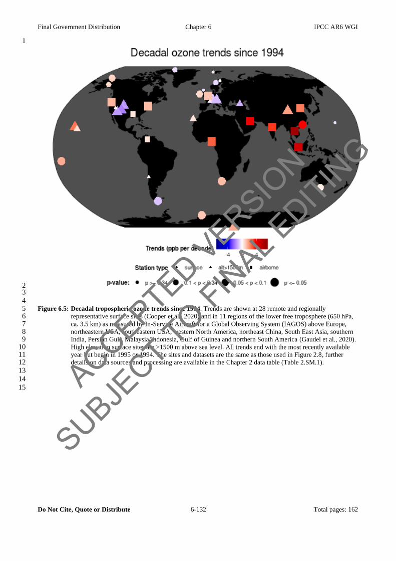
Final Government Distribution Chapter 6 IPCC AR6 WGI
Do Not Cite, Quote or Distribute 6-132 Total pages: 162
1
2 3
4 Figure 6.5: Decadal tropospheric ozone trends since 1994. Trends are shown at 28 remote and regionally 5
representative surface sites (Cooper et al., 2020) and in 11 regions of the lower free troposphere (650 hPa, 6 ca. 3.5 km) as measured by In-Service Aircraft for a Global Observing System (IAGOS) above Europe, 7 northeastern USA, southeastern USA, western North America, northeast China, South East Asia, southern 8 India, Persian Gulf, Malaysia/Indonesia, Gulf of Guinea and northern South America (Gaudel et al., 2020). 9 High elevation surface sites are >1500 m above sea level. All trends end with the most recently available 10 year but begin in 1995 or 1994. The sites and datasets are the same as those used in Figure 2.8, further 11 details on data sources and processing are available in the Chapter 2 data table (Table 2.SM.1). 12
13
14
15 ACCEPTED VERSION
SUBJECT TO FIN
AL EDITIN
G

Final Government Distribution Chapter 6 IPCC AR6 WGI
Do Not Cite, Quote or Distribute 6-133 Total pages: 162
1
ACCEPTED VERSION
SUBJECT TO FIN
AL EDITIN
G

Final Government Distribution Chapter 6 IPCC AR6 WGI
Do Not Cite, Quote or Distribute 6-134 Total pages: 162
1 Figure 6.6: Long term climatological mean (a) and time evolution (b) of tropospheric NO2 vertical column 2
density from the merged GOME/SCIAMACHY/GOME-2 (TM4NO2A version 2.3) dataset for the 3 period 1996-2016 (Georgoulias et al., 2019). Time evolution of NO2 column shown in panel (b) is 4 normalized to the fitted 1996 levels for the 10 regions shown as boxes in panel (a). Further details on data 5 sources and processing are available in the chapter data table (Table 6.SM.1). 6
7
8
9
ACCEPTED VERSION
SUBJECT TO FIN
AL EDITIN
G

Final Government Distribution Chapter 6 IPCC AR6 WGI
Do Not Cite, Quote or Distribute 6-135 Total pages: 162
1
2 3
Figure 6.7: Distribution of PM2.5 composition mass concentration (in μg m–3) for the major PM2.5 aerosol 4 components. Those aerosol components are sulfate, nitrate, ammonium, sodium, chloride, organic 5 carbon, and elemental carbon. The central world map depicts the intermediate level regional breakdown 6 of observations (10 regions) following the IPCC Sixth Assessment Report Working Group III (AR6 7 WGIII). Monthly averaged PM2.5 aerosol component measurements are from: (i) the Environmental 8 Protection Agency (EPA) network which include 211 monitor sites primarily in urban areas of North 9 America during 2000-2018 (Solomon et al., 2014) (ii) the Interagency Monitoring of Protected Visual 10 Environments (IMPROVE) network during 2000-2018 over 198 monitoring sites representative of the 11 regional haze conditions over North America, (iii) the European Monitoring and Evaluation Programme 12 (EMEP) network over 70 monitoring in Europe and (eastern) Eurasia during 2000-2018, (iv) the Acid 13 Deposition Monitoring Network in East Asia (EANET) network with 39 (18 remote, 10 rural, 11 urban) 14 sites in Eurasia, Eastern Asia, South-East Asia and Developing Pacific, and Asia-Pacific Developed 15 during 2001-2017, (v) the global Surface Particulate Matter Network (SPARTAN) during 2013-2019 16 with sites primarily in highly populated regions around the world (i.e, North America, Latin America and 17 Caribbean, Africa, Middle East, Southern Asia, Eastern Asia, South-Eastern Asia and Developing 18 Pacific) (Snider et al., 2015, 2016), and (vii) individual observational field campaign averages over Latin 19 America and Caribbean, Africa, Europe, Eastern Asia, and Asia-Pacific Developed (Celis et al., 2004; 20 Feng et al., 2006; Bourotte et al., 2007; Fuzzi et al., 2007; Mariani and de Mello, 2007; Molina et al., 21 2007; Favez et al., 2008; Mkoma, 2008; Aggarwal and Kawamura, 2009; Mkoma et al., 2009; de Souza 22 et al., 2010; Li et al., 2010; Martin et al., 2010; Molina et al., 2010; Radhi et al., 2010; Weinstein et al., 23 2010; Batmunkh et al., 2011; Gioda et al., 2011; Pathak et al., 2011; Zhang et al., 2012; Cho and Park, 24 2013; Zhao et al., 2013; Wang et al., 2019; Kuzu et al., 2020). Further details on data sources and 25 processing are available in the chapter data table (Table 6.SM.1). 26
27
ACCEPTED VERSION
SUBJECT TO FIN
AL EDITIN
G

Final Government Distribution Chapter 6 IPCC AR6 WGI
Do Not Cite, Quote or Distribute 6-136 Total pages: 162
1
2 3
4 Figure 6.8: Time evolution of changes in global mean aerosol optical depth (AOD) at 550 nm. Year of reference 5
is 1850. Data shown from individual Coupled Model Intercomparison Project Phase 6 (CMIP6) historical 6 simulations. Each time series corresponds to the ensemble mean of realizations done by each model. 7 Simulation results from years including major volcanic eruptions, e.g. Novarupta (1912) and Pinatubo 8 (1991), are excluded from the analysis for models encompassing the contribution of stratospheric 9 volcanic aerosols to total AOD. Further details on data sources and processing are available in the chapter 10 data table (Table 6.SM.1). 11
12
13
ACCEPTED VERSION
SUBJECT TO FIN
AL EDITIN
G

Final Government Distribution Chapter 6 IPCC AR6 WGI
Do Not Cite, Quote or Distribute 6-137 Total pages: 162
1 2 Figure 6.9: Time evolution of global annual mean tropospheric hydroxyl (OH) over the historical period, 3
expressed as a percentage anomaly relative to the mean over 1998-2007. a) Results from three CMIP6 4 models, including UKESM1-0LL (green), GFDL-ESM4 (blue), and CESM2-WACCM (red), are shown; 5 the shaded light green and light red bands show mean over multiple ensemble members for UKESM1-6 0LL (3) and CESM2-WACCM (3) models, respectively with the multi-model mean anomalies shown in 7 thick black line. b) multimodel mean OH anomalies for 1980-2015 period compared with those derived 8 from observational-based inversions from (Montzka et al., 2011; Rigby et al., 2017; Turner et al., 2017; 9 Nicely et al., 2018; Naus et al., 2019; Patra et al., 2021) in the zoomed box. Further details on data 10 sources and processing are available in the chapter data table (Table 6.SM.1). 11
12
13
14 ACCEPTED VERSIO
N
SUBJECT TO FIN
AL EDITIN
G

Final Government Distribution Chapter 6 IPCC AR6 WGI
Do Not Cite, Quote or Distribute 6-138 Total pages: 162
1 2
Figure 6.10: Multi-model mean Effective radiative forcings (ERFs) due to aerosol changes between 1850 and 3 recent-past (1995-2014). Panel (a) shows the spatial distribution of the net ERF with area-weighted 4 global mean ERF shown at the lower right corner. Uncertainty is represented using the advanced 5 approach: No overlay indicates regions with robust signal, where ≥66% of models show change greater 6 than variability threshold and ≥80% of all models agree on sign of change; diagonal lines indicate regions 7 with no change or no robust signal, where <66% of models show a change greater than the variability 8 threshold; crossed lines indicate regions with conflicting signal, where ≥66% of models show change 9
ACCEPTED VERSION
SUBJECT TO FIN
AL EDITIN
G

Final Government Distribution Chapter 6 IPCC AR6 WGI
Do Not Cite, Quote or Distribute 6-139 Total pages: 162
greater than variability threshold and <80% of all models agree on sign of change. For more information 1 on the advanced approach, please refer to the Cross-Chapter Box Atlas.1. Panel (b) shows the mean 2 shortwave and longwave ERF for each of the 14 regions defined in the Atlas. Violins in panel (b) show 3 the distribution of values over regions where ERFs are significant. ERFs are derived from the difference 4 between top of the atmosphere (TOA) radiative fluxes for Aerosol Chemistry Model Intercomparison 5 Project (AerChemMIP) experiments histSST and histSST-piAer (Collins et al., 2017) averaged over 1995-6 2014 (Box 1.4, Chapter 1). The results come from 7 Earth System Models: MIROC6, MPI-I-ESM-1-2-7 HAM, MRI-ESM2-0, GFDL-ESM4, GISS-E2-1-G, NorESM2-LM, and UKESM-0-LL. These data can 8 be seen in the Interactive Atlas. Further details on data sources and processing are available in the chapter 9 data table (Table 6.SM.1). 10
11
12
ACCEPTED VERSION
SUBJECT TO FIN
AL EDITIN
G

Final Government Distribution Chapter 6 IPCC AR6 WGI
Do Not Cite, Quote or Distribute 6-140 Total pages: 162
1 2 Figure 6.11: Time evolution of 20-year multi-model mean averages of the annual area-weighted mean regional 3
net Effective Radiative Forcings (ERFs) due to aerosols for each of the 14 major regions in the Atlas, 4 and global mean, using the models and model experiments as in Figure 6.10. Further details on data 5 sources and processing are available in the chapter data table (Table 6.SM.1). 6
7
8
ACCEPTED VERSION
SUBJECT TO FIN
AL EDITIN
G

Final Government Distribution Chapter 6 IPCC AR6 WGI
Do Not Cite, Quote or Distribute 6-141 Total pages: 162
1
2 3 Figure 6.12: Contribution to effective radiative forcing (ERF) (left) and global mean surface air temperature 4
(GSAT) change (right) from component emissions between 1750 to 2019 based on CMIP6 models 5 (Thornhill et al., 2021). ERFs for the direct effect of well-mixed greenhouse gases (WMGHGs) are from 6 the analytical formulae in section 7.3.2, H2O (strat) is from Table 7.8. ERF for other components are 7 multi-model means from Thornhill et al. (2021) and are based on ESM simulations in which emissions of 8 one species at a time are increased from 1850 to 2014 levels. The derived emission-based ERFs are 9 rescaled to match the concentration-based ERFs in Figure 7.6. Error bars are 5-95% and for the ERF 10 account for uncertainty in radiative efficiencies and multi-model error in the means. ERF due to aerosol-11 radiation (ERFari) and cloud effects are calculated from separate radiation calls for clear-sky and aerosol 12 free conditions (Ghan, 2013; Thornhill et al., 2021). “Cloud” includes cloud adjustments (semi-direct 13 effect) and ERF from indirect aerosol-cloud to -0.22 W m-2 for ERFari and -0.84 W m-2 interactions 14 (ERFaci). The aerosol components (SO2, organic carbon, black carbon) are scaled to sum to -0.22 W m-2 15 for ERFari and -0.84 W m-2 for “cloud” (section 7.3.3). For GSAT estimates, time series (1750-2019) for 16 the ERFs have been estimated by scaling with concentrations for WMGHGs and with historical emissions 17 for SLCFs. The time variation of ERFaci for aerosols is from Chapter 7. The global mean temperature 18 response is calculated from the ERF time series using an impulse response function (see Cross-Chapter 19 Box 7.1) with a climate feedback parameter of -1.31 W m-2 C-1. Further details on data sources and 20 processing are available in the chapter data table (Table 6.SM.1). 21
22 23 24
25
26
27
28 ACCEPTED VERSION
SUBJECT TO FIN
AL EDITIN
G

Final Government Distribution Chapter 6 IPCC AR6 WGI
Do Not Cite, Quote or Distribute 6-142 Total pages: 162
1 Figure 6.13: Multi-model mean surface air temperature response due to aerosol changes between 1850 and 2
recent-past (1995-2014) calculated as the difference between CMIP6 ‘historical’ and AerChemMIP 3 ‘hist-piAer’ experiments, where a) is the spatial pattern of the annual mean surface air temperature 4 response, and b) is the mean zonally averaged response. Model means are derived from years 1995-2014. 5 Uncertainty is represented using the advanced approach: No overlay indicates regions with robust signal, 6 where ≥66% of models show change greater than variability threshold and ≥80% of all models agree on 7 sign of change; diagonal lines indicate regions with no change or no robust signal, where <66% of models 8 show a change greater than the variability threshold; crossed lines indicate regions with conflicting signal, 9 where ≥66% of models show change greater than variability threshold and <80% of all models agree on 10 sign of change. For more information on the advanced approach, please refer to the Cross-Chapter Box 11 Atlas.1. AerChemMIP models MIROC6, MRI-ESM2-0, NorESM2-LM, GFDL-ESM4, GISS-E2-1-G, 12 UKESM1-0-LL are used in the analysis. Further details on data sources and processing are available in 13 the chapter data table (Table 6.SM.1). 14
15
16
ACCEPTED VERSION
SUBJECT TO FIN
AL EDITIN
G
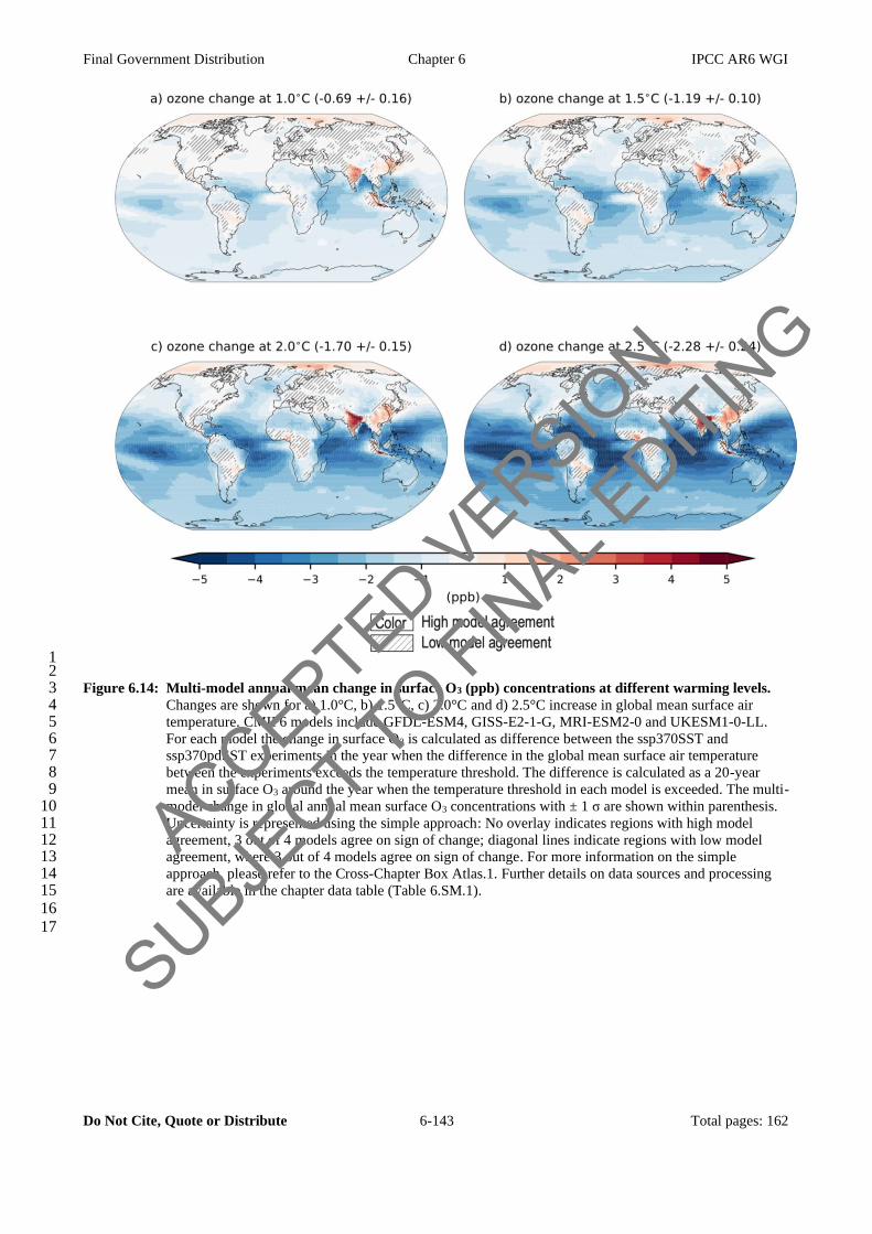
Final Government Distribution Chapter 6 IPCC AR6 WGI
Do Not Cite, Quote or Distribute 6-143 Total pages: 162
1 2 Figure 6.14: Multi-model annual mean change in surface O3 (ppb) concentrations at different warming levels. 3
Changes are shown for a) 1.0°C, b) 1.5°C, c) 2.0°C and d) 2.5°C increase in global mean surface air 4 temperature. CMIP6 models include GFDL-ESM4, GISS-E2-1-G, MRI-ESM2-0 and UKESM1-0-LL. 5 For each model the change in surface O3 is calculated as difference between the ssp370SST and 6 ssp370pdSST experiments in the year when the difference in the global mean surface air temperature 7 between the experiments exceeds the temperature threshold. The difference is calculated as a 20-year 8 mean in surface O3 around the year when the temperature threshold in each model is exceeded. The multi-9 model change in global annual mean surface O3 concentrations with ± 1 σ are shown within parenthesis. 10 Uncertainty is represented using the simple approach: No overlay indicates regions with high model 11 agreement, 3 out of 4 models agree on sign of change; diagonal lines indicate regions with low model 12 agreement, where 3 out of 4 models agree on sign of change. For more information on the simple 13 approach, please refer to the Cross-Chapter Box Atlas.1. Further details on data sources and processing 14 are available in the chapter data table (Table 6.SM.1). 15
16
17
ACCEPTED VERSION
SUBJECT TO FIN
AL EDITIN
G

Final Government Distribution Chapter 6 IPCC AR6 WGI
Do Not Cite, Quote or Distribute 6-144 Total pages: 162
1
2
3 4 Figure 6.15: Global mean surface air temperature (GSAT) response to an abrupt reduction in emissions (at time 5
t=0) of idealized climate forcing agents with different lifetimes. All emissions are cut to give a 6 radiative forcing of -1 W m-2 at steady state (except for CO2). In other words, if the yearly emissions are 7 E0 before the reduction, they will have a fixed lower value Eyear>0 = (E0 - ΔE) for all succeeding years. For 8 comparison, the GSAT response to a sustained reduction in CO2 emissions resulting in an RF of -1 W m-2 9 in year 100 is included (dashed line). The temperature response is calculated using an impulse response 10 function (see Cross-Chapter Box 7.1) with a climate feedback parameter of -1.31 W m-2 C-1. Further 11 details on data sources and processing are available in the chapter data table (Table 6.SM.1). 12
13
14 ACCEPTED VERSION
SUBJECT TO FIN
AL EDITIN
G

Final Government Distribution Chapter 6 IPCC AR6 WGI
Do Not Cite, Quote or Distribute 6-145 Total pages: 162
1
2 3
4 Figure 6.16: Global-mean temperature response 10 and 100 years following one year of present-day (year 2014) 5
emissions. The temperature response is broken down by individual species and shown for total 6 anthropogenic emissions (top), sectoral emissions (left) and regional emissions (right). Sectors and 7 regions are sorted by (high-to-low) net temperature effect on the 10-year time scale. Error bars in the top 8 panel show uncertainty (5-95% interval) in net temperature effect due to uncertainty in radiative forcing 9 only (calculated using a Monte Carlo approach and best estimate uncertainties from the literature - see 10 Lund et al. (Lund et al., 2020) for details). CO2 emissions are excluded from open biomass burning and 11 residential biofuel use due to their unavailability in CEDS and uncertainties around non-sustainable 12 emission fraction. Emissions for 2014 originate from the Community Emissions Data System (CEDS) 13 (Hoesly et al., 2018), except for HFCs which are from Purohit et al. (2020), open biomass burning from 14 van Marle et al. (2017), and aviation H2O which is from Lee et al.(2020). The split of fossil fuel 15 production and distribution and combustion for energy and residential and commercial fuel use into fossil 16 fuel and biofuel components obtained from the GAINS model (ECLIPSE version 6b dataset). Open 17 biomass burning emissions are not included for the regions. Emission are aggregated into fossil fuel 18 production and distribution (coal mining, oil and gas production, upstream gas flaring, gas distribution 19 networks), agriculture (livestock and crop production), fossil fuel combustion for energy (power plants), 20 industry (combustion and production processes, solvent use losses from production and end use), 21 residential and commercial (fossil fuel use for cooking and heating as well is HFCs leakage from A/C and 22 refrigeration), waste management (solid waste, incl. landfills and open trash burning, residential and 23 industrial waste water), transport (road and off-road vehicles, and HFC leakage from A/C and 24 refrigeration equipment), residential and commercial (biofuels use for cooking and heating), open 25 biomass burning (forest, grassland, savannah fires, and agricultural waste burning), shipping (incl. 26 international shipping), and aviation (incl. international aviation). Further details on data sources and 27 processing are available in the chapter data table (Table 6.SM.1). 28
29
30
ACCEPTED VERSION
SUBJECT TO FIN
AL EDITIN
G

Final Government Distribution Chapter 6 IPCC AR6 WGI
Do Not Cite, Quote or Distribute 6-146 Total pages: 162
1
2 Figure 6.17: Emission source-sector attribution of regional population weighted mean concentrations of PM2.5 3
and ozone for present day emissions (year 2014). Regional concentrations and source apportionment 4 calculated with the TM5-FASST model (Van Dingenen et al., 2018) for the 2014 emission data from the 5 Community Emissions Data System (CEDS) (Hoesly et al., 2018) and van Marle et al.(2017) for open 6 biomass burning. PM2.5 dust and seasalt are monthly mean climatological average over 2010-2018 from 7 CAMS global reanalysis (EAC4) (Inness et al., 2019), generated using Copernicus Climate Change 8 Service information [January 2020]. Anthropogenic sectors are similar to those in Figures 6.2 and 6.16 9 except grouping of fossil fuel production, distribution and combustion for energy under “Energy” and 10 grouping of use of fossil fuel and biofuel use for cooking and heating under “Residential and 11 Commercial”. Further details on data sources and processing are available in the chapter data table (Table 12 6.SM.1). 13
14
ACCEPTED VERSION
SUBJECT TO FIN
AL EDITIN
G

Final Government Distribution Chapter 6 IPCC AR6 WGI
Do Not Cite, Quote or Distribute 6-147 Total pages: 162
1
2
3 Figure 6.18: Global anthropogenic and biomass burning short-lived climate forcer (SLCF) and CO2 emissions 4
from 1850 to 2100 and HFC emissions from 1990 to 2100. Emissions for the Coupled Model 5 Intercomparison Project Phase 6 (CMIP6) for the period 1850-2014 are based on Hoesly et al. (2018) and 6 van Marle et al. (2017), emissions for CMIP5 for the period 1850-2005 are from Lamarque et al. (2010), 7 CO2 emissions are from EDGAR database (Crippa et al., 2020); CH4 and HFCs are from (Crippa et al., 8 2019); and air pollutants are from (EC-JRC / PBL, 2020), Höglund-Isaksson (2012) and Klimont et al. 9 (2017) for ECLIPSE. Projections originate from the Shared Socio-Economic Pathway (SSP) database 10 (Riahi et al., 2017; Rogelj et al., 2018; Gidden et al., 2019), Representative Concentration Pathway (RCP) 11 database (van Vuuren et al., 2011), GAINS (CLE – current legislation baseline without Kigali 12 Amendment, KA – Kigali Amendment, MTFR – maximum technical mitigation potential) for HFCs 13 (Purohit et al., 2020), Velders et al. (2015), ECLIPSE (Stohl et al., 2015). Further details on data sources 14 and processing are available in the chapter data table (Table 6.SM.1). 15
16
17
ACCEPTED VERSION
SUBJECT TO FIN
AL EDITIN
G

Final Government Distribution Chapter 6 IPCC AR6 WGI
Do Not Cite, Quote or Distribute 6-148 Total pages: 162
1
2 3
4 Figure 6.19: Regional anthropogenic and biomass burning short-lived climate forcer (SLCF) emissions from 5
1850 to 2100. Emissions for the Coupled Model Intercomparison Project Phase 6 (CMIP6) for the period 6 1850-2014 are based on Hoesly et al. (2018) and van Marle et al. (2017) and emissions for CMIP5 for 7 the period 1850-2005 are from Lamarque et al. (2010). Projections originate from the Shared Socio-8
ACCEPTED VERSION
SUBJECT TO FIN
AL EDITIN
G

Final Government Distribution Chapter 6 IPCC AR6 WGI
Do Not Cite, Quote or Distribute 6-149 Total pages: 162
Economic Pathway (SSP) database (Riahi et al., 2017; Rogelj et al., 2018; Gidden et al., 2019) and 1 Representative Concentration Pathway (RCP) database (van Vuuren et al., 2011). Further details on data 2 sources and processing are available in the chapter data table (Table 6.SM.1). 3
4
ACCEPTED VERSION
SUBJECT TO FIN
AL EDITIN
G

Final Government Distribution Chapter 6 IPCC AR6 WGI
Do Not Cite, Quote or Distribute 6-150 Total pages: 162
1
2 3 Figure 6.20: Projected changes in regional annual mean surface ozone (O3) (ppb) from 2015 to 2100 in different 4
shared socio-economic pathways (SSPs). Each panel represents values averaged over the corresponding 5 land area (except for Global) shown on the map in Figure 6.7. Solid colored lines and shading indicate the 6 multi-model mean and ±1 σ across the available CMIP6 models (Turnock et al. 2020; Allen et al. 2021) 7 for each scenario. Changes are relative to annual mean values calculated over the period 2005-2014 from 8 the historical experiment as indicated in the top left of each regional panel along with ±1 σ. For each 9 model all available ensemble members are averaged before being used to calculate the multi-model mean. 10 Ozone changes are also displayed in the Interactive Atlas. Further details on data sources and processing 11 are available in the chapter data table (Table 6.SM.1). 12 13
14 ACCEPTED VERSION
SUBJECT TO FIN
AL EDITIN
G

Final Government Distribution Chapter 6 IPCC AR6 WGI
Do Not Cite, Quote or Distribute 6-151 Total pages: 162
1
2 3
4 Figure 6.21: Future changes in regional 5-year mean surface PM2.5 from 2015 to 2100 in different shared socio-5
economic pathways (SSPs). PM2.5 stands for micrograms per cubic meter of aerosols with diameter less 6 than 2.5 μm and is calculated by summing up individual aerosol mass components from each model as: 7 black carbon + particulate organic matter + sulphate + 0.25 * sea salt + 0.1 * dust. Since not all CMIP6 8 models reported nitrate aerosol, it is not included here. See Figure 6.20 for further details. PM2.5 changes 9 are also displayed in the Interactive Atlas. Further details on data sources and processing are available in 10 the chapter data table (Table 6.SM.1). 11
12
13
14 ACCEPTED VERSION
SUBJECT TO FIN
AL EDITIN
G

Final Government Distribution Chapter 6 IPCC AR6 WGI
Do Not Cite, Quote or Distribute 6-152 Total pages: 162
1 2 Figure 6.22: Time evolution of the effects of short-lived climate forcers (SLCFs) and hydrofluorocarbons 3
(HFCs) on global surface air temperature (GSAT) across the WGI core set of Shared Socio-4 Economic Pathways (SSPs). Effects of net aerosols, methane, tropospheric ozone and 5 hydrofluorocarbons (HFCs) (with lifetimes <50years), and the sum of these, relative to year 2019 and to 6 year 1750. The GSAT changes are based on the assessed historic and future evolution of Effective 7 Radiative Forcing (Section 7.3.5). The temperature responses to the ERFs are calculated with an impulse 8 response function with an equilibrium climate sensitivity of 3.0°C for a doubling of atmospheric CO2 9 (feedback parameter of -1.31 W m-2 C-1, see CC-Box 7.1). The vertical bars to the right in each panel 10 show the uncertainties (5-95% ranges) for the GSAT change between 2019 and 2100. Further details on 11 data sources and processing are available in the chapter data table (Table 6.SM.1). 12
ACCEPTED VERSION
SUBJECT TO FIN
AL EDITIN
G

Final Government Distribution Chapter 6 IPCC AR6 WGI
Do Not Cite, Quote or Distribute 6-153 Total pages: 162
1 2 Figure 6.23: Contribution from regional emissions of short-lived climate forcers (SLCFs) to changes in global 3
surface air temperature (GSAT) in 2040 (upper row) and 2100 (lower row), relative to 2020 for 4 four Shared Socio-economic Pathways (SSP). Adapted from (Lund et al., 2020). NOx, CO, and VOC 5 account for the impact through changes in ozone and methane, NOx additionally includes the impact 6 through formation of nitrate aerosols. BC, SO2 and OC accounts for the direct aerosol effect (aerosol-7 radiation interactions), as well as an estimate of the semi-direct effect for BC due to rapid adjustments 8 and indirect effect (aerosol-cloud interactions) of sulfate aerosols. Regions are the same as shown in the 9 map in Figure 6.7. Further details on data sources and processing are available in the chapter data table 10 (Table 6.SM.1). 11
12
13
14 ACCEPTED VERSION
SUBJECT TO FIN
AL EDITIN
G

Final Government Distribution Chapter 6 IPCC AR6 WGI
Do Not Cite, Quote or Distribute 6-154 Total pages: 162
1
2
3 Figure 6.24: Effects of short-lived climate forcers (SLCFs) and hydrofluorocarbons (HFCs) on global surface air 4
temperature (GSAT) across the WGI core set of Shared Socio-Economic Pathways (SSPs). Effects 5 of net aerosols, methane, tropospheric ozone, and hydrofluorocarbons (HFCs; with lifetimes <50years), 6 are compared with those of total anthropogenic forcing for 2040 and 2100 relative to year 2019. The 7 GSAT changes are based on the assessed historic and future evolution of Effective Radiative Forcing 8 (Section 7.3.5). The temperature responses to the ERFs are calculated with an impulse response function 9 with an equilibrium climate sensitivity of 3.0°C for a doubling of atmospheric CO2 (feedback parameter 10 of -1.31 W m-2 C-1, see Cross-Chapter Box 7.1). Uncertainties are 5-95% ranges. The scenario total (grey 11 bar) includes all anthropogenic forcings (long- and short-lived climate forcers, and land use changes) 12 whereas the white points and bars show the net effects of SLCFs and HFCs and their uncertainties. 13 Further details on data sources and processing are available in the chapter data table (Table 6.SM.1). 14
15
16
ACCEPTED VERSION
SUBJECT TO FIN
AL EDITIN
G

Final Government Distribution Chapter 6 IPCC AR6 WGI
Do Not Cite, Quote or Distribute 6-155 Total pages: 162
1 2 Figure 6.25: Effect of dedicated air pollution or climate policy on population-weighted PM2.5 concentrations (µg 3
m-3) and share of population (%) exposed to different PM2.5 levels across selected world regions. 4 Thresholds of 10 µg m-3 and 35 µg m-3 represent the WHO air quality guideline and the WHO interim 5 target 1, respectively; WHO (2017). Results are compared for SSP3-7.0 (no major improvement of 6 current legislation is assumed), SSP3-LowSLCF (strong air pollution controls are assumed), and a climate 7
0
20
40
60
0
20
40
60
80
100
2015 2030 2050 2100
0
20
40
60
0
20
40
60
80
100
2015 2030 2050 2100
0
20
40
60
0
20
40
60
80
100
2015 2030 2050 2100
0
20
40
60
0
20
40
60
80
100
2015 2030 2050 2100
0
20
40
60
0
20
40
60
80
100
2015 2030 2050 2100
0
20
40
60
0
20
40
60
80
100
2015 2030 2050 2100
0
20
40
60
0
20
40
60
80
100
2015 2030 2050 2100
0
20
40
60
0
20
40
60
80
100
2015 2030 2050 2100
0
20
40
60
0
20
40
60
80
100
2015 2030 2050 2100
0
20
40
60
0
20
40
60
80
100
2015 2030 2050 2100
0
20
40
60
0
20
40
60
80
100
2015 2030 2050 2100
0
20
40
60
0
20
40
60
80
100
2015 2030 2050 2100
0
20
40
60
0
20
40
60
80
100
2015 2030 2050 2100
0
20
40
60
0
20
40
60
80
100
2015 2030 2050 2100
0
20
40
60
0
20
40
60
80
100
2015 2030 2050 2100
0
20
40
60
0
20
40
60
80
100
2015 2030 2050 2100
0
20
40
60
0
20
40
60
80
100
2015 2030 2050 2100
0
20
40
60
0
20
40
60
80
100
2015 2030 2050 2100
0
20
40
60
0
20
40
60
80
100
2015 2030 2050 21000
20
40
60
0
20
40
60
80
100
2015 2030 2050 2100
0
20
40
60
0
20
40
60
80
100
2015 2030 2050 2100
0
20
40
60
0
20
40
60
80
100
2015 2030 2050 2100
0
20
40
60
0
20
40
60
80
100
2015 2030 2050 2100
0
20
40
60
0
20
40
60
80
100
2015 2030 2050 2100
0
20
40
60
0
20
40
60
80
100
2015 2030 2050 2100
0
20
40
60
0
20
40
60
80
100
2015 2030 2050 2100
0
20
40
60
0
20
40
60
80
100
2015 2030 2050 2100
0
20
40
60
0
20
40
60
80
100
2015 2030 2050 2100
0
20
40
60
0
20
40
60
80
100
2015 2030 2050 2100
Africa
Asia-Pacific Developed
Eastern Asia
Europe
North America
Southern Asia
Latin America & Caribbean
Middle East
South-East Asia & developping Pacific
Eurasia
population
exposed
(%)
Population
weighted mean
concentration
(μg m–3 )
35 μg m–3
10 μg m–3
Thresholds
for population
exposure
SSP3 7.0 No climate mitigationWeak air pollution Control
SSP3 7.0 low SLCF low CH4
No climate mitigationStrong Air pollution Control
SSP3 3.4Strong Climate MitigationWeak air pollution Control
Surface PM2.5
0
20
40
60
0
20
40
60
80
100
2015 2030 2050 2100
ACCEPTED VERSION
SUBJECT TO FIN
AL EDITIN
G

Final Government Distribution Chapter 6 IPCC AR6 WGI
Do Not Cite, Quote or Distribute 6-156 Total pages: 162
mitigation scenario SSP3-3.4; details of scenario assumptions are discussed in Riahi et al. (2017) and Rao 1 et al. (2017). Analysis performed with the TM5-FASST model (Van Dingenen et al., 2018) using 2 emission projections from the Shared Socio-Economic Pathway (SSP) database (Riahi et al., 2017; 3 Rogelj et al., 2018; Gidden et al., 2019). Further details on data sources and processing are available in 4 the chapter data table (Table 6.SM.1). 5
6 7
8
ACCEPTED VERSION
SUBJECT TO FIN
AL EDITIN
G

Final Government Distribution Chapter 6 IPCC AR6 WGI
Do Not Cite, Quote or Distribute 6-157 Total pages: 162
1
2 3 Figure 6.26: Effect of dedicated air pollution or climate policy on population-weighted ozone concentrations 4
(SOMO0; ppb) and share of population (%) exposed to chosen ozone levels across ten world 5 regions. Results are compared for SSP3-7.0 (no major improvement of current legislation is assumed), 6
0
20
40
60
80
100
0
20
40
60
80
100
2015 2030 2050 2100
0
20
40
60
80
100
0
20
40
60
80
100
2015 2030 2050 2100
0
20
40
60
80
100
0
20
40
60
80
100
2015 2030 2050 2100
0
20
40
60
80
100
0
20
40
60
80
100
2015 2030 2050 2100
0
20
40
60
80
100
0
20
40
60
80
100
2015 2030 2050 2100
0
20
40
60
80
100
0
20
40
60
80
100
2015 2030 2050 2100
0
20
40
60
80
100
0
20
40
60
80
100
2015 2030 2050 2100
0
20
40
60
80
100
0
20
40
60
80
100
2015 2030 2050 2100
0
20
40
60
80
100
0
20
40
60
80
100
2015 2030 2050 2100
0
20
40
60
80
100
0
20
40
60
80
100
2015 2030 2050 2100
0
20
40
60
80
100
0
20
40
60
80
100
2015 2030 2050 2100
0
20
40
60
80
100
0
20
40
60
80
100
2015 2030 2050 2100
0
20
40
60
80
100
0
20
40
60
80
100
2015 2030 2050 2100
0
20
40
60
80
100
0
20
40
60
80
100
2015 2030 2050 2100
0
20
40
60
80
100
0
20
40
60
80
100
2015 2030 2050 2100
0
20
40
60
80
100
0
20
40
60
80
100
2015 2030 2050 2100
0
20
40
60
80
100
0
20
40
60
80
100
2015 2030 2050 2100
0
20
40
60
80
100
0
20
40
60
80
100
2015 2030 2050 2100
0
20
40
60
80
100
0
20
40
60
80
100
2015 2030 2050 2100
0
20
40
60
80
100
0
20
40
60
80
100
2015 2030 2050 2100
0
20
40
60
80
100
0
20
40
60
80
100
2015 2030 2050 2100
0
20
40
60
80
100
0
20
40
60
80
100
2015 2030 2050 2100
0
20
40
60
80
100
0
20
40
60
80
100
2015 2030 2050 2100
0
20
40
60
80
100
0
20
40
60
80
100
2015 2030 2050 2100
0
20
40
60
80
100
0
20
40
60
80
100
2015 2030 2050 2100
0
20
40
60
80
100
0
20
40
60
80
100
2015 2030 2050 2100
0
20
40
60
80
100
0
20
40
60
80
100
2015 2030 2050 2100
Population weighted mean
SOMO0 [sum of maximum 8-hour O3 levels]
(ppb)
60 pbb
35 ppb
Surface O3
0
20
40
60
80
100
0
20
40
60
80
100
2015 2030 2050 2100
0
20
40
60
80
100
0
20
40
60
80
100
2015 2030 2050 2100
population
exposed
(%)
Thresholds
for population
exposure
SSP3 7.0 No climate mitigationWeak air pollution Control
SSP3 7.0 low SLCF low CH4
No climate mitigationStrong Air pollution Control
SSP3 3.4Strong Climate MitigationWeak air pollution Control
Africa
Asia-Pacific Developed
Eastern Asia
Europe
North America
Southern Asia
Latin America & Caribbean
Middle East
South-East Asia & developping Pacific
Eurasia
0
20
40
60
80
100
0
20
40
60
80
100
2015 2030 2050 2100
ACCEPTED VERSION
SUBJECT TO FIN
AL EDITIN
G

Final Government Distribution Chapter 6 IPCC AR6 WGI
Do Not Cite, Quote or Distribute 6-158 Total pages: 162
SSP3-LowSLCF (strong air pollution controls are assumed), and a climate mitigation scenario (SSP3-1 3.4); details of scenario assumptions are discussed in Riahi et al. (2017) and Rao et al. (2017). Analysis 2 performed with the TM5-FASST model (Van Dingenen et al., 2018) using emission projections from the 3 Shared Socio-Economic Pathway (SSP) database [https://tntcat.iiasa.ac.at/SspDb/dsd] (Riahi et al., 2017; 4 Rogelj et al., 2018; Gidden et al., 2019). Further details on data sources and processing are available in 5 the chapter data table (Table 6.SM.1). 6
7
8
9
10
11
ACCEPTED VERSION
SUBJECT TO FIN
AL EDITIN
G

Final Government Distribution Chapter 6 IPCC AR6 WGI
Do Not Cite, Quote or Distribute 6-159 Total pages: 162
1 2 Box 6.1, Figure 1: Knowledge exchange between laboratory/theoretical studies, observations and global 3
chemistry-climate models to inform our understanding of short-lived climate forcers (SLCFs). 4 5
6
ACCEPTED VERSION
SUBJECT TO FIN
AL EDITIN
G

Final Government Distribution Chapter 6 IPCC AR6 WGI
Do Not Cite, Quote or Distribute 6-160 Total pages: 162
1 2 Cross-Chapter Box 6.1, Figure 1: Emission reductions and their effect on aerosols and climate in response to 3
COVID-19. Estimated reductions in emissions of CO2, SO2 and NOx are shown in 4 panel (a) based on reconstructions using activity data (updated from Forster et al., 5 2020). Eight Earth System Models (ESMs) performed multiple ensemble 6 simulations of the response to COVID-19 emissions reductions forced with these 7 assumed emission reductions up till August 2020 followed by a constant 8 continuation near the August value to the end of 2020. Emission reductions were 9 applied relative to the SSP2-4.5 scenario. Panel (b) shows ESM simulated AOD at 10 550nm (only seven models reported this variable). Panel (c) shows ESM simulated 11 GSAT anomalies during 2020; curves denote the ensemble mean result for each 12 model with shading used for ±1 standard deviation for each model. ESM data from 13 these simulations (“ssp245-covid”) is archived on the Earth System Grid CMIP6 14 database. Uncertainty is represented using the simple approach: No overlay 15 indicates regions with high model agreement, where ≥80% of models agree on sign 16 of change; diagonal lines indicate regions with low model agreement, where <80% 17 of models agree on sign of change. For more information on the simple approach, 18 please refer to the Cross-Chapter Box Atlas.1. 19
20 21 22
23
24 ACCEPTED VERSION
SUBJECT TO FIN
AL EDITIN
G

Final Government Distribution Chapter 6 IPCC AR6 WGI
Do Not Cite, Quote or Distribute 6-161 Total pages: 162
1
2 3 FAQ 6.1, Figure 1: Main short-lived climate forcers, their sources, how long they exist in the atmosphere, and 4
their relative contribution to global surface temperature changes between 1750 and 2019 (area 5 of the globe). By definition, this contribution depends on the lifetime, the warming/cooling potential 6 (radiative efficiency), and the emissions of each compound in the atmosphere. Blue indicates 7 cooling and orange warming. Note that, between 1750 and 2019, the cooling contribution from 8 aerosols (blue diamonds and globe) was approximately half the warming contribution from carbon 9 dioxide. 10
11
ACCEPTED VERSION
SUBJECT TO FIN
AL EDITIN
G

Final Government Distribution Chapter 6 IPCC AR6 WGI
Do Not Cite, Quote or Distribute 6-162 Total pages: 162
1 FAQ6.2, Figure 1: Links between actions aiming to limit climate change and actions to improve air 2
quality. Greenhouse gases and aerosols (orange and blue) can affect directly climate. Air 3 pollutants (bottom) can affect the human health, ecosystems and climate. All these compounds 4 have common sources and sometimes interact with each other in the atmosphere which makes 5 impossible to consider them separately (dotted grey arrows). 6
7
8
ACCEPTED VERSION
SUBJECT TO FIN
AL EDITIN
G