P1.64 ASSESSING THE PERFORMANCE OF A PROGNOSTIC AND A DIAGNOSTIC CLOUD SCHEME USING

SINGLE COLUMN MODEL SIMULATIONS OF TWP-ICE

Charmaine N. Franklin * Centre for Australian Weather and Climate Research

A partnership between CSIRO and the Australian Bureau of Meteorology, Aspendale, Victoria, Australia Christian Jakob

School of Mathematical Sciences, Monash University, Clayton, Victoria, Australia Martin Dix, Alain Protat, Greg Roff

Centre for Australian Weather and Climate Research, Aspendale and Melbourne, Victoria, Australia

1. INTRODUCTION

The Tropical Warm Pool International Cloud Experiment (TWP-ICE, May et al. 2008) was a major field campaign held in the Darwin area of Northern Australia in January and February 2006. One of the main aims of the experiment was to provide boundary conditions and validation data for modeling studies to help facilitate model development with a focus on tropical convection and clouds. The Darwin area experiences a wide array of convective systems consisting of active monsoon periods with typical maritime storms and break periods with more coastal and continental convection. The observations collected during the TWP-ICE campaign allow for a detailed evaluation of the ability of numerical models to simulate the evolution of tropical cloud systems and their effect on the environment. Global climate models (GCMs) must be able to represent cloud-scale processes and the feedbacks between clouds and the large-scale environment to ensure accurate projections of climate change.

The primary aim of the work presented here is to use the single column model (SCM) approach with a version of the UK Met Office SCM to assess the ability of two fundamentally different parameterizations of clouds to reproduce the observed thermodynamic and cloud structures as well as the associated radiative fluxes during the TWP-ICE experiment. The two model versions used are based on the Met Office model where one version uses a new generation prognostic cloud scheme (Wilson et al. 2008a) while the other employs the current (or control) diagnostic scheme used routinely in the model (Smith, 1990). 2. EXPERIMENT DESIGN

The Australian Community Climate Earth System Simulator (ACCESS) is a new coupled climate and earth system model that is being developed as a joint initiative between the Australian Bureau of Meteorology and CSIRO in partnership with Australian * Corresponding author address: Charmaine N. Franklin, CSIRO Marine and Atmospheric Sciences, Private Bag No. 1, Aspendale, VIC Australia 3195; e-mail: charmaine.franklin@csiro.au

universities. The model provides a framework for numerical weather prediction and studies of climate change and enables research into processes occurring in the earth system (for information on the modeling system see http://www.accessimulator.org.au/). As part of the ACCESS project this model needs to be extensively validated in the Australian region. The recent intensive field campaign of TWP-ICE has produced a new data set for model evaluation and as such is an ideal case study for the ACCESS model. 2.1 Description of the ACCESS/UM SCM The ACCESS SCM used in this study is the Unified Model (UM) version 7.1 with 38 vertical levels, and is based on the second version of the Hadley Centre Global Environment Model (HadGEM2) described in Collins et al. (2008). The new prognostic cloud scheme that has been developed for the UM includes prognostic variables for the cloud liquid water content, the cloud ice water content, the bulk cloud fraction, the liquid cloud fraction and the ice cloud fraction. Diagnostic cloud schemes such as the Smith (1990) scheme are relatively simple in their representation of cloud properties and exhibit strongly constrained relationships between cloud variables. Representing changes in the prognostic cloud variables from each physical process in the model allows a way to directly link the cloud condensate and cloud fraction together and consistently simulate the effects of physical processes in a much more complete and realistic way than a diagnostic scheme (Wilson et al. 2008a). 2.2 TWP-ICE Forcing and Validation data

The large-scale single-column model forcing and evaluation data set was derived from the constrained variational objective analysis approach described in Zhang and Lin (1997) and Zhang et al. (2001) using the observations taken during TWP-ICE (Xie et al. 2009). The aim of the objective analysis is to make minimum adjustments to the original sounding data to constrain the wind, temperature and humidity fields to satisfy conservation of mass, moisture, energy and momentum through a variational technique. The constraint variables used are surface pressure, surface latent and sensible heat fluxes, wind stress, precipitation, net radiation at the surface and top of the

atmosphere, and variability of total column water content. The method takes into account measurement uncertainties and it has been shown that the magnitude of the adjustments required to meet conservation is comparable to these uncertainties (Zhang and Lin 1997).

The observational forcing dataset has a temporal resolution of 3 hours and the data needed to force the SCM has been linearly interpolated to 30 minutes, which is the timestep used in the SCM simulations. The model is initialized once on 19 January 2006 and then run for 25 days. The lower boundary condition used in the SCM experiments is a prescribed sea surface temperature (SST), where the model then calculates the turbulent fluxes of sensible and latent heat at the surface. Three-dimensional advective tendencies are specified as forcing from the variational objective analysis and the model horizontal wind fields are relaxed back to those observed over 3 hour periods. 3. MODEL EVALUATION The Darwin ARM site has a suite of active remote sensing instruments that provide vertical cloud structure information. The Active Remotely Sensed

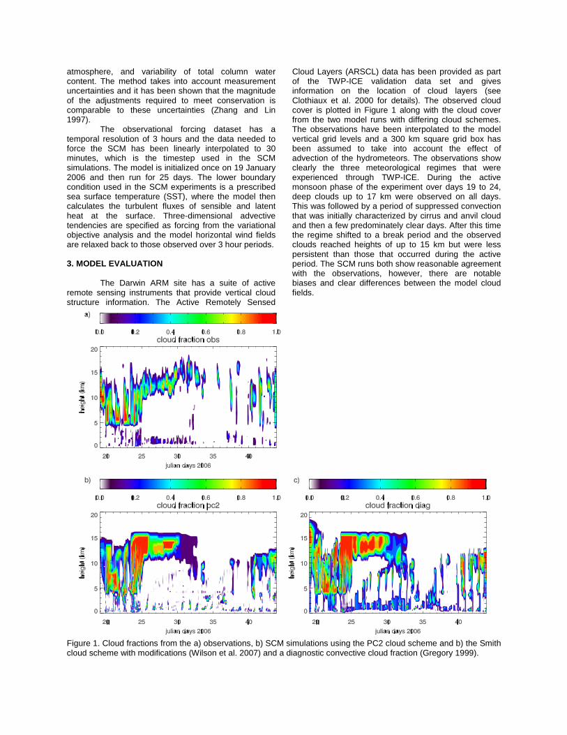
Cloud Layers (ARSCL) data has been provided as part of the TWP-ICE validation data set and gives information on the location of cloud layers (see Clothiaux et al. 2000 for details). The observed cloud cover is plotted in Figure 1 along with the cloud cover from the two model runs with differing cloud schemes. The observations have been interpolated to the model vertical grid levels and a 300 km square grid box has been assumed to take into account the effect of advection of the hydrometeors. The observations show clearly the three meteorological regimes that were experienced through TWP-ICE. During the active monsoon phase of the experiment over days 19 to 24, deep clouds up to 17 km were observed on all days. This was followed by a period of suppressed convection that was initially characterized by cirrus and anvil cloud and then a few predominately clear days. After this time the regime shifted to a break period and the observed clouds reached heights of up to 15 km but were less persistent than those that occurred during the active period. The SCM runs both show reasonable agreement with the observations, however, there are notable biases and clear differences between the model cloud fields.

Figure 1. Cloud fractions from the a) observations, b) SCM simulations using the PC2 cloud scheme and b) the Smith cloud scheme with modifications (Wilson et al. 2007) and a diagnostic convective cloud fraction (Gregory 1999).

3.1 The Active Monsoon Period (Julian Days 19-24)

During the active monsoon phase the models produce similar cloud distributions to the observations, however, the modeled clouds tend to penetrate higher than those observed. The SCM run with the diagnostic cloud scheme initially produces deeper clouds than the run with the prognostic scheme (see Fig. 1). The diagnostic cloud scheme uses an interpolation method to calculate the area cloud fraction (Cusack 1999). This parameterization divides each model layer into three sublayers and the

large-scale cloud scheme is then called on each of these sublayers. These are assumed to be maximally overlapped with each other. The prognostic scheme on the other hand, sets the area cloud fraction equal to the volume cloud fraction calculated on the 38 model levels. This difference makes the comparison between the cloud schemes difficult, however we choose to use the Cusack scheme as this is used in HadGEM2 and these results then contribute to the analysis of that widely used model. Over days 23 – 25 when a mesoscale convective system was present in the experiment domain, both cloud schemes produce significantly higher cloud cover than the observations.

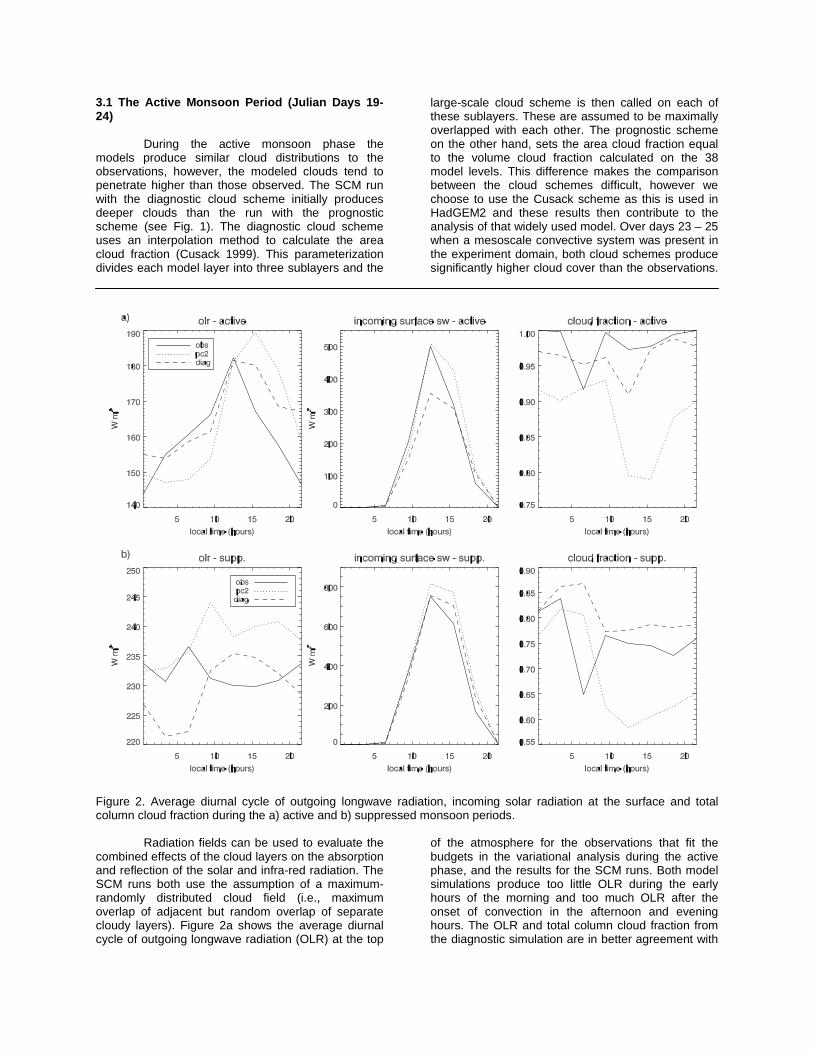
Figure 2. Average diurnal cycle of outgoing longwave radiation, incoming solar radiation at the surface and total column cloud fraction during the a) active and b) suppressed monsoon periods.

Radiation fields can be used to evaluate the combined effects of the cloud layers on the absorption and reflection of the solar and infra-red radiation. The SCM runs both use the assumption of a maximum-randomly distributed cloud field (i.e., maximum overlap of adjacent but random overlap of separate cloudy layers). Figure 2a shows the average diurnal cycle of outgoing longwave radiation (OLR) at the top

of the atmosphere for the observations that fit the budgets in the variational analysis during the active phase, and the results for the SCM runs. Both model simulations produce too little OLR during the early hours of the morning and too much OLR after the onset of convection in the afternoon and evening hours. The OLR and total column cloud fraction from the diagnostic simulation are in better agreement with

the observations than those from the PC2 simulation. For both of these variables the amplitude of the diurnal cycle is larger in the PC2 run than in the observations, while the diagnostic run produces lower diurnal cycle amplitudes than the observations. The reduction in OLR during the afternoon and evening hours is better captured with the prognostic cloud scheme, however, the timing is too late and the amplitude too high by 7 W m-2. The increase in OLR during the morning is well captured by the diagnostic scheme, while the PC2 simulation shows a delay. Many of these differences are due to the way in which the prognostic and diagnostic cloud schemes interact with the cumulus parameterization. In PC2 the convection scheme detrains condensate directly into the grid box thereby allowing the stratiform cloud

scheme to reflect details of the convective clouds. This differs from the diagnostic scheme where the detrained condensate evaporates and the radiative effect of the convective cloud is represented by a separate diagnostic cloud category.

The diurnal cycle of incoming solar radiation at the surface is well simulated by the prognostic cloud scheme while the diagnostic scheme underestimates the solar radiation at the surface by up to 150 W m-2. The largest errors from the prognostic scheme simulation in the representation of the incoming shortwave radiation occur immediately after the peak at local noon. This model does not reduce the incoming shortwave radiation enough at the time when convection is beginning to occur in the early afternoon.

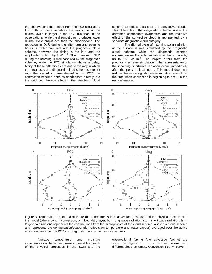
Figure 3. Temperature (a, c) and moisture (b, d) increments from advection (obs/adv) and the physical processes in the model (where conv = convection, bl = boundary layer, lw = long wave radiation, sw = short wave radiation, lsr = large-scale rain and represents the contributions from the microphysics of the cloud scheme, and cld = cloud scheme and represents the condensation/evaporation effects on temperature and water vapour) averaged over the active monsoon period for the PC2 and diagnostic cloud schemes, respectively.

Average temperature and moisture increments over the active monsoon period from each of the physical processes in the SCM and the

observational forcing (the advective forcing) are shown in Figure 3 for the two simulations with different cloud schemes. Convection (“conv” curve in

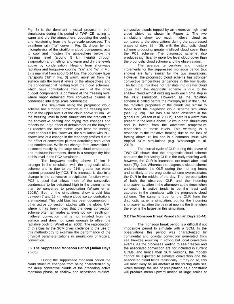
Fig. 3) is the dominant physical process in both simulations during this period of TWP-ICE, acting to warm and dry the atmosphere, opposing the cooling and moistening from the large-scale processes. The stratiform rain (“lsr” curve in Fig. 3), driven by the microphysics of the stratiform cloud component, acts to cool and moisten the atmosphere below the freezing level (around 5 km height) through evaporation and melting, and warm and dry the levels above by condensation. Heating from shortwave radiation and longwave cooling (“sw” and “lw” in Fig. 3) is maximal from about 5-14 km. The boundary layer transports (“bl” in Fig. 3) warm, moist air from the surface into the lowest levels of the atmosphere and the condensational heating from the cloud schemes, which have contributions from each of the other budget components is dominant at the freezing level where vapor detrained from convective plumes is condensed into large scale condensate.

The simulation using the prognostic cloud scheme has stronger convection at the freezing level and in the upper levels of the cloud above 11 km. At the freezing level in both simulations the gradient of the convective heating and drying rate changes and reflects the large effect of detrainment as the buoyant air reaches the more stable layer near the melting level at about 5 km. However, the simulation with PC2 shows less of a change in the tendency profiles due to the effect of convective plumes detraining both vapor and condensate. While this change from convection is balanced mostly by the large scale cloud temperature and moisture increments, there is a stronger dry bias at this level in the PC2 simulation.

The longwave cooling above 12 km is stronger in the simulation with the prognostic cloud scheme and is due to the 21% greater ice water content produced by PC2. This increase is due to a change in the convective precipitation function when PC2 is used that allows more of the convective condensate to be detrained high in the plume rather than be converted to precipitation (Wilson et al. 2008b). Both of the simulations show a cold bias between 7 and 15 km where cloud ice concentrations are maximal. This cold bias has been documented in other active convection studies with the global UM, where it has been noted that the deep convection scheme often terminates at levels too low, resulting in midlevel convection that is not initiated from the surface and does not warm enough to offset the radiative cooling (Willett et al. 2008). The reproduction of this bias by the SCM gives credence to the use of this methodology to examine the performance of the physical parameterizations in simulations of tropical convection. 3.2 The Suppressed Monsoon Period (Julian Days 25-35) During the suppressed monsoon period the cloud structure changed from being characterized by the deep convective clouds of the preceding active monsoon phase, to shallow and occasional midlevel

convective clouds topped by an extensive high level cloud shield as shown in Figure 1. The two simulations show too much midlevel cloud as compared to the observations during the suppressed phase of days 25 – 35, with the diagnostic cloud scheme producing greater midlevel cloud cover than the PC2 scheme. The diagnostic scheme also produces significantly more low level cloud cover than the prognostic cloud scheme and the observations.

The average temperature and moisture increments for the suppressed monsoon period (not shown) are fairly similar for the two simulations. However, the prognostic cloud scheme has stronger convective temperature tendencies in the low levels. The fact that this does not translate into greater cloud cover than the diagnostic scheme is due to the shallow cloud almost drizzling away each time step in the PC2 simulation. However, as the radiation scheme is called before the microphysics in the SCM, the radiative properties of the clouds are similar to those from the diagnostic cloud scheme simulation (see Fig. 2b). This has also been observed in the global UM (Wilson et al. 2008b). There is a warm bias present in the levels above 12 km in both simulations and is forced from the advective temperature tendencies at these levels. This warming is a response to the radiative heating due to the lack of forcing above 16 km and is a common issue with tropical SCM simulations (e.g. Woolnough et al. 2010).

The diurnal cycle of OLR during this phase of TWP-ICE shows that the prognostic cloud scheme captures the increasing OLR in the early morning well, however, the OLR is increased too much after local noon (Fig. 2b). Whereas the diagnostic cloud scheme underestimates the OLR during the morning hours and similarly to the prognostic scheme overestimates the OLR in the middle of the day. The representation of both the observed OLR and the incoming shortwave radiation in the afternoon at the times when convection is active tends to be the least well captured in the simulation with the prognostic cloud scheme. The same is true for the OLR from the diagnostic scheme simulation, but for the incoming shortwave radiation the peak at noon is the time when the error is the largest in this simulation.

3.2 The Monsoon Break Period (Julian Days 36-44) The monsoon break period is a difficult if not impossible period to simulate with a SCM. In the observations this period was characterized by continental and coastal convection generated from sea breezes resulting in strong but local convective events. As the processes leading to sea-breezes and the associated convection are not included in current GCMs, and hence their SCM versions, the models cannot be expected to simulate convection and the associated cloud fields realistically. If they do so, this will most likely be an artefact of the forcing data set, which through the use of precipitation as a constraint will produce mean upward motion at large scales at

the time of rainfall, when it is clear from the observations that this motion was strongly focused in coastal and island sea-breezes (see May et al., 2008). For the reasons above, we refrain from an in-depth discussion of the results for this period. 4. COMPARISON OF CLOUD VARIABILITY BETWEEN THE PROGNOSTIC AND DIAGNOSTIC CLOUD SCHEMES To explore the variability in the cloud fields that the SCM is able to simulate Figure 4 shows the area cloud fractions averaged over three hour periods during the active period as a function of the relative humidity at four different heights. The observed relative humidity has been calculated from the observed/analysis temperature and specific humidity fields using the same equations that are used in the model to calculate the saturation mixing ratio. For temperatures above 0°C vapor saturation pressure

over water is used and below this temperature the saturation is calculated over ice. Figure 4a shows that at 2 km the relationship between cloud fraction and relative humidity is similar between the models, with PC2 simulating a wider range of cloud fractions across a larger range of relative humidities. PC2 produces more occurrences of cloud fraction below 0.03 than the diagnostic scheme, which is more in line with the observations at this height. The models produce too many clouds with cloud fractions greater than 0.2 and the modeled cloud fractions have a larger dependence on relative humidity than the observations. During the active phase both simulations produce a negative relative humidity bias in the levels below 8 km and a positive bias above. This bias of positive relative humidity in the upper regions of convective clouds and a negative bias below agrees with that found by Petch et al. (2007) in their study using the UM to simulate active and suppressed convection.

Figure 4. Three hourly averages of cloud area fraction during the active monsoon period plotted as a function of relative humidity at four different heights for the observations (asterisk), prognostic (circle) and diagnostic (square) cloud schemes.

At 5km the PC2 simulation and the observations produce a greater frequency of cloud fractions below 0.2 than the diagnostic cloud scheme. Figure 4c shows that at 11 km neither of the cloud schemes capture the same amount of variability that the observations show, however, the bulk of cloud occurrence at this height is well represented by both schemes.

At 15 km the SCM produces cloud fractions that tend to be higher than the observations. The

diagnostic cloud scheme shows a fairly tight relationship between cloud fraction and relative humidity, which is different to the observations and the prognostic cloud scheme. PC2 at this height generates a limited range of cloud fractions and shows a large jump to high cloud fractions once the relative humidity reaches saturation, something that is not observed.

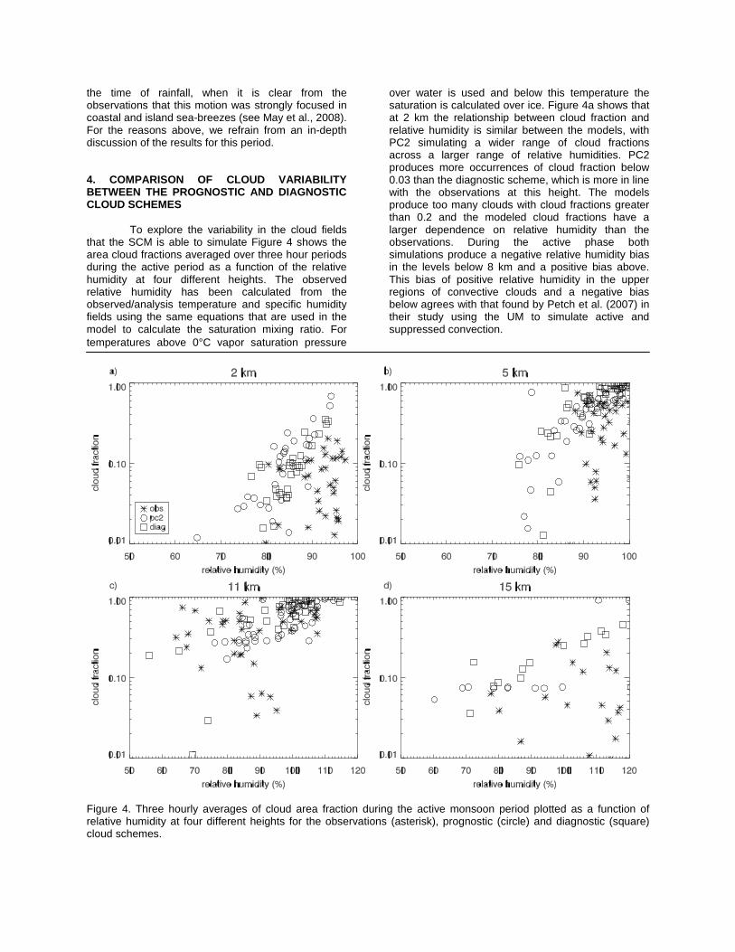
Figure 5. As for Figure 4 except for the suppressed monsoon phase of TWP-ICE.

Cloud fractions at 2 km during the suppressed phase (see Figure 5a) tend to occur at lower relative humidities and lower cloud fractions than during the active period. These low-level cloud properties are better simulated with PC2 as the diagnostic scheme predicts cloud fractions that are larger than those observed. Figure 5b shows that at 5 km the diagnostic cloud scheme is not able to simulate the observed clouds with low cloud fractions at low relative humidities. The prognostic scheme on the other hand, captures this phase space well but has too many occurrences of cloud at this height, particularly at relative humidities less than 20%. At 11

km this bias reverses and PC2 does not simulate enough cloud with cloud fractions below 0.1, a bias also seen with the diagnostic cloud scheme. This height coincides with the base of the cirrus cloud and both cloud schemes produce similar distributions of cloud fractions, with the diagnostic scheme shifted to cloud occurring at lower relative humidities than in the PC2 simulation.

At 15 km, which corresponds to one model level below cloud top, the diagnostic scheme shows a tighter relationship with relative humidity than the prognostic scheme though both produce clouds with higher cloud fractions than those observed. PC2 tends to produce clouds at lower relative humidities

than the diagnostic scheme and tends to produce clusters of cloud fractions that appear independent of

relative humidity, as was also seen at this height in the active phase (see Fig. 4d).

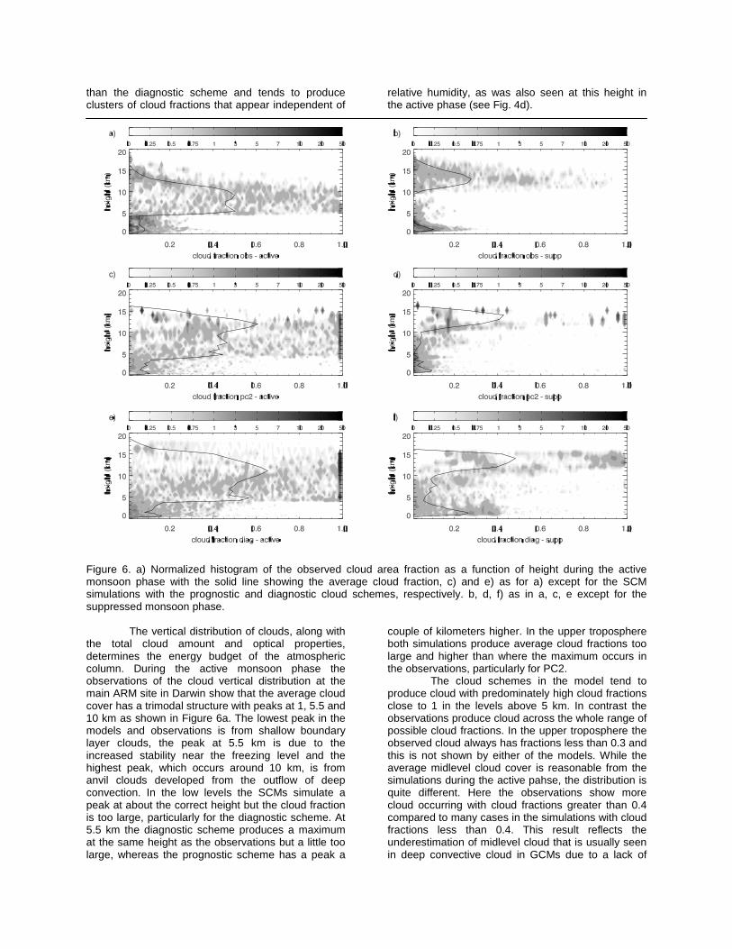
Figure 6. a) Normalized histogram of the observed cloud area fraction as a function of height during the active monsoon phase with the solid line showing the average cloud fraction, c) and e) as for a) except for the SCM simulations with the prognostic and diagnostic cloud schemes, respectively. b, d, f) as in a, c, e except for the suppressed monsoon phase. The vertical distribution of clouds, along with the total cloud amount and optical properties, determines the energy budget of the atmospheric column. During the active monsoon phase the observations of the cloud vertical distribution at the main ARM site in Darwin show that the average cloud cover has a trimodal structure with peaks at 1, 5.5 and 10 km as shown in Figure 6a. The lowest peak in the models and observations is from shallow boundary layer clouds, the peak at 5.5 km is due to the increased stability near the freezing level and the highest peak, which occurs around 10 km, is from anvil clouds developed from the outflow of deep convection. In the low levels the SCMs simulate a peak at about the correct height but the cloud fraction is too large, particularly for the diagnostic scheme. At 5.5 km the diagnostic scheme produces a maximum at the same height as the observations but a little too large, whereas the prognostic scheme has a peak a

couple of kilometers higher. In the upper troposphere both simulations produce average cloud fractions too large and higher than where the maximum occurs in the observations, particularly for PC2.

The cloud schemes in the model tend to produce cloud with predominately high cloud fractions close to 1 in the levels above 5 km. In contrast the observations produce cloud across the whole range of possible cloud fractions. In the upper troposphere the observed cloud always has fractions less than 0.3 and this is not shown by either of the models. While the average midlevel cloud cover is reasonable from the simulations during the active pahse, the distribution is quite different. Here the observations show more cloud occurring with cloud fractions greater than 0.4 compared to many cases in the simulations with cloud fractions less than 0.4. This result reflects the underestimation of midlevel cloud that is usually seen in deep convective cloud in GCMs due to a lack of

detrainment from the cumulus parameterization at these levels, and was documented in a recent study of the global forecast UM by Bodas-Salcedo et al. (2008).

During the suppressed monsoon phase the peak cloud fraction in the simulations is again too large and occurs at a greater height than the observations. The low level cloud is overestimated by the diagnostic scheme but well represented by the prognostic scheme. During these times the models show too much midlevel cloud. Again the high level cloud in the models tends to have cloud fractions greater than 0.5, which is not seen in the observations. 5. ICE CLOUD PROPERTIES DURING DAYS 25-30 Observations of ice water content and fall velocity have been obtained from a radar-lidar retrieval (Delanoë and Hogan 2008; Protat et al.

2009) for days 25-30 of the suppressed monsoon phase. Figure 7a shows that when ice is present, the models systematically underestimate the amount observed. Note that the ice content is a prognostic variable in both simulations and the amounts are similar in the upper levels that correspond to the anvil cloud generated from the deep convection during the active phase. The levels below 8 km show a much larger amount of ice in the simulation with the prognostic cloud scheme, which is in better agreement with the observations. This difference between the prognostic and diagnostic cloud scheme results reflects the differences in how the cloud schemes interact with the convection scheme and the tuning to the convective precipitation function. The distribution of ice water content shown in Fig. 7b shows that the prognostic scheme produces more variability in ice amounts but both simulations underestimate the amount seen in the observations.

Figure 7. a) Profiles of ice water content (log (g m-3)) over days 25-30, b) the PDF of ice water content, c) profiles of ice fall velocity (m s-1) and d) the PDF of the ice fall velocity.

The fall velocity of ice decreases as the height at which it occurs increases in both the model

and the observations, with the diagnostic cloud scheme showing a gradient closest to the

observations in the levels below 8 km. The observations have been converted from the reflectivity-weighted fall speed to the mass-weighted fall speed so as to match the model results. The conversion applied assumes that the reflectivity-weighted fall speed is 1.4 times the mass-weighted fall speed, however there will be some variability in this linear conversion based on the properties of the ice clouds changing with height (Matrosov and Heymsfield 2000). This larger fall speed from the prognostic cloud scheme compared to the diagnostic scheme reflects the increase in the amount of ice water content in the levels below 8 km in the PC2 simulation since the mean fall speed in the models is a function of the total ice water content.

The majority of the ice falls with velocities between 25 and 30 cm s-1 in both the models and the observations, however, the models both show larger skewness and kurtosis in their PDFs of ice fall velocity. Ice occurs with fall speeds between 25 – 30 cm s-1 in the observations with a probability of occurrence of 0.15 compared to 0.39 in the diagnostic scheme simulation and 0.25 in the prognostic scheme simulation. The distribution from the simulation with the diagnostic cloud scheme is bimodal with a secondary peak at 50 – 55 cm s-1, which is not seen in the observations. The prognostic scheme distribution of ice fall speeds is more representative of the observations than the diagnostic scheme in terms of the skewness, however, the results from this simulation show that the model is at times producing fall speeds that are much larger than those observed and simulated by the model using the diagnostic scheme. The maximum fall speed simulated by the prognostic scheme is about twice that observed. 6. SUMMARY The ACCESS SCM, which is the UM SCM of the UK Met Office, has been run for the TWP-ICE case to investigate the ability of the model to represent the vertical distribution and temporal evolution of tropical cloud systems. This SCM study has shown that the TWP-ICE case is interesting and useful for model evaluation and development due to the varying nature of the convection during the experiment and the extensive observational dataset. Of particular appeal in the data set is the availability of observations at both the large and cloud scales.

Two SCM runs have been analyzed each using a different representation of clouds. The simulations both produced generally reasonable representations of the TWP-ICE cloud fields, with the three different observed cloud regimes captured by the model. The average diurnal cycle of OLR over the active phase was better simulated with the diagnostic cloud scheme, however, the prognostic scheme PC2 produced a significantly better average diurnal cycle of incoming shortwave radiation at the surface. Both cloud schemes produced average diurnal cycles of OLR during the suppressed monsoon phase that were quite different to that observed, with the prognostic

scheme having larger errors in the middle of the day and the diagnostic scheme in the early morning hours. Both models produced a much larger amplitude of the diurnal cycle of OLR during the suppressed phase that than observed.

The prognostic scheme is able to simulate more variable cloud fields in agreement with the observations as demonstrated by the relationship of cloud fraction with relative humidity. The diagnostic cloud scheme produced cloud fractions that were shown to be more dependent on the relative humidity than the observations and the cloud fractions from the prognostic cloud scheme. Both cloud schemes produced most clouds with cloud fractions close to 1 during the active phase in the levels above 4 km. This is in contrast to the observations that show a more equal spread in cloud fraction occurrence from 5 to 12 km and above this level all clouds observed had cloud fractions less than 0.3. Similarly during the suppressed phase the observations of clouds in the upper troposphere show very little cloud occurring with fractions greater than 0.6. The diagnostic cloud scheme, however, mostly produces cloud fractions above 0.8 at these heights and the prognostic scheme simulates clouds across the whole range of cloud fractions.

Ice water contents and fall velocities during the first 5 days of the suppressed period show that when ice water is present in the models the amount is underestimated, however the majority of ice occurring in the simulations falls with similar fall speeds to those observed. The average profiles of the ice fall speeds show that in the levels above 13 km the model fall speeds are faster than those observed even though the ice water content at these levels is less. In the levels below 8 km the diagnostic cloud scheme generally produces ice with slower fall speeds than the observations, however, the prognostic scheme fall speeds are faster than those observed with the maximum ice fall speed from the PC2 simulation being about twice that observed.

Lin et al. (2004) suggested that the inability of many models to simulate realistic representations of the MJO may be caused by systematic diabatic heating profile errors. Temperature and moisture errors in the SCM simulations were the most pronounced during the suppressed period. Other studies such as Li et al. (2008) have identified the link between poor simulations of suppressed convection leading to unrealistic simulations of sub-seasonal variability in tropical convection, including the MJO, and TWP-ICE may provide a good case to study the model biases and make improvements in the model cloud and convection parameterizations. The GEWEX Cloud Systems Study Group (GCSS) is currently running a TWP-ICE intercomparison project for both SCMs and CRMs. The GCSS project uses the forcing and evaluation data set that was used in this study and the outcomes from the high resolution models will enable a more rigorous assessment of the link between the cloud scheme and the convection parameterization in the ACCESS/UM SCM and the

ability of the model to simulate tropical cloud system. This is intended to build on the results reported herein and lead to improvements to the physical parameterizations.

Acknowledgements This work was supported by the Australian Department of Climate Change. CJ is grateful for support from the U.S. Department of Energy under grant DE-FG02-03ER63533 as part of the Atmospheric Radiation Measurement Program (ARM). Data were obtained from the ARM program sponsored by the U.S. Department of Energy, Office of Science, Office of Biological and Environmental Research, Environmental Sciences Division. The forcing data were generated by Shaocheng Xie from the Lawrence Livermore National Laboratory. The radar-lidar retriwevals used in this study were generated by Julien Delanoë from the University of Reading. CNF would like to acknowledge Damian Wilson and Jon Petch from the Met Office for discussions and insight on PC2. References Bodas-Salcedo, A., M.J. Webb, M.E. Brooks, M.A. Ringer, K.D. Williams, S.F. Milton and D.R. Wilson, 2008. Evaluating cloud systems in the Met Office global forecast model using simulated CloudSat radar reflectivities. J. Geophys. Res., 113, doi:10.1029/2007JD009620. Clothiaux, E.E., T.P. Ackerman, G.G. Mace, K.P. Moran, R.T. Marchand, M.A. Miller and B.E. Martner, 2000. Objective determination of cloud heights and radar reflectivities using a combination of active remote sensors at the ARM CART sites. J. Appl. Meteor., 39, 645-665. Collins, W., N. Bellouin, M. Doutriaux-Boucher, T. Hinton, C.D. Jones, S. Fiddicoat, G. Martin, F. O’Connor, J. Rae, S. Reddy, C. Senior, I. Totterdell, and S. Woodard, 2008: Evaluation of the HadGEM2-ES model. Hadley Centre Technical Note 74, 43pp. Available online at http://www.metoffice.gov.uk/research/hadleycentre/pubs/HCTN/index.html Cusack, S., 1999: Estimating the subgrid variance of saturation and its parametrization for use in a GCM cloud scheme. Q. J. R. Meteorol. Soc., 125, 3057-3076 Delanoë J and Hogan R., 2008: A variational scheme for retrieving ice cloud properties from combined radar, lidar and infrared radiometer. J. Geophys. Res., 113, D07204, doi:10.1029/2007JD009000. Gregory, J. 1999: Representation of the radiative effects of convective anvils. Hadley Centre Tech. Note 7. Met. Office, Exeter, UK.

Li, C., X. Jia, J. Ling, W. Zhou and C. Zhang, 2008. Sensitivity of MJO simulations to diabatic heating profiles. Clim. Dynam., doi 10.1007/s00382-008-0455-x Lin, J.-L., B. Mapes, M. Zhang and M. Newman, 2004. Stratiform precipitation, vertical heating profiles and the Madden-Julian oscillation. J. Atmos. Sci., 61, 296-309. May, P.T., J.H. Mather, G. Vaughan, C.N. Jakob, G.M. McFarquhar, K.N. Bower and G.G. Mace, 2008. The Tropical Warm Pool International Cloud Experiment (TWP-ICE). Bull. Amer. Meteor. Soc., 89, 629-645. Petch, J.C., M. Willett, R.Y. Wong and S.J. Woolnough, 2007: Modelling suppressed and active convection. Comparing a numerical weather prediction, cloud-resolving and single-column model. Q. J. R. Meteorol. Soc., 133, 1087-1100. Protat, A., J. Delanoë, A. Plana-Fattori, P. T. May, and E. O'Connor, 2009: The statistical properties of tropical ice clouds generated by the West-African and Australian monsoons from ground-based radar-lidar observations. Quart. J. Roy. Meteor. Soc., 136(S1), 345-363, 2010, doi: 10.1002/qj.490. Smith, R.N.B. 1990. A scheme for predicting layer clouds and their water contents in a general circulation model. Q. J. R. Meteorol. Soc., 116, 435-460. Willett, M.R., P. Bechtold, D.L. Williamson, J.C. Petch, S.F. Milton and S.J. Woolnough, 2008: Modelling suppressed and active convection: Comparisons between three global atmospheric models. Q. J. R. Meteorol. Soc., 134, 1881-1896. Wilson, D.R., R.N.B. Smith, D. Gregory, C.A. Wilson, A.C. Bushell, and S. Cusack, 2007: The large-scale cloud scheme and saturated specific humidity. Unified Model documentation paper 26. Met. Office, Exeter, UK Wilson, D.R., A.C. Bushell, A.M. Kerr-Munslow, D. Price and C. Morcrette, 2008a. PC2: A prognostic cloud fraction and condensation scheme. Part I: Scheme description. Q. J. R. Meteorol. Soc., 134, 2093-2107. Wilson, D.R., A.C. Bushell, A.M. Kerr-Munslow, D. Price, C. Morcrette and A. Bodas-Salcedo, 2008b. PC2: A prognostic cloud fraction and condensation scheme. Part II: Results of climate model simulations. Q. J. R. Meteorol. 134, 2109-2125. Woolnough, S.J., P.N. Blossey, K.-M. Xu, P. Bechtold, J.-P. Chaboureau, T. Hosomi, S.F. Iacobellis, Y. Luo, J.C. Petch, R.Y. Wong and S. Xie, 2010: Modelling of

convective processes during the suppressed phase of a Madden-Julian oscillation: Comparing single-column models with cloud resolving models. Q. J. R. Meteorol. Soc., 136, 333-353. Xie, S., T. Hume, C. Jakob, S.A. Klein, R. McCoy and M. Zhang, 2009: Observed large-scale structures and diabatic heating and drying profiles during TWP-ICE. J. Climate, 23, 57-79. Zhang, M.H. and J.L. Lin, 1997. Constrained variational analysis of sounding data based on column-integrated budgets of mass, heat, moisture and momentum: Approach and application to ARM measurements. J. Atmos. Sci., 54, 1503-1524. Zhang, M.H., J.L. Lin, R.T.. Cederwall, J.J. Yio and S.C. Xie, S.C. 2001. Objective analysis of ARM IOP data: Method and sensitivity. Mon. Wea. Rev.,129, 295-311.