p-winds: an open-source Python code to model planetary

Astronomy & Astrophysics manuscript no. 42038 ©ESO 2021December 21, 2021

p-winds: An open-source Python code to model planetary outflowsand upper atmospheres?

Leonardo A. Dos Santos1, 2, Aline A. Vidotto3, 4, Shreyas Vissapragada5, Munazza K. Alam6, 7, Romain Allart8,Vincent Bourrier2, James Kirk6, Julia V. Seidel2, 9, and David Ehrenreich2

1 Space Telescope Science Institute, 3700 San Martin Drive, Baltimore, MD 21218, USAe-mail: [email protected]

2 Observatoire astronomique de l’Université de Genève, Chemin Pegasi 51, 1290 Versoix, Switzerland3 Leiden Observatory, Leiden University, Postbus 9513, 2300 RA Leiden, The Netherlands4 School of Physics, Trinity College Dublin, the University of Dublin, College Green, Dublin-2, Ireland5 Division of Geological and Planetary Sciences, California Institute of Technology, 1200 East California Blvd, Pasadena, CA 91125,

USA6 Center for Astrophysics | Harvard & Smithsonian, 60 Garden Street, Cambridge, MA 02138, USA7 Earth and Planets Laboratory, The Carnegie Institution for Science, 5241 Broad Branch Road, Washington, DC 20015, USA8 Department of Physics, and Institute for Research on Exoplanets, Université de Montréal, Montréal, H3T 1J4, Canada9 European Southern Observatory, Alonso de Córdova 3107, Santiago, Casilla 19001, Chile

Received 17 August 2021; accepted 30 November 2021

ABSTRACT

Atmospheric escape is considered to be one of the main channels for evolution in sub-Jovian planets, particularly in their early lives.While there are several hypotheses proposed to explain escape in exoplanets, testing them with atmospheric observations remains achallenge. In this context, high-resolution transmission spectroscopy of transiting exoplanets for the metastable helium triplet (He 23S)at 1 083 nm has emerged as a reliable technique for observing and measuring escape. To aid in the prediction and interpretation ofmetastable He transmission spectroscopy observations, we developed the code p-winds. This is an open-source, fully documented,scalable Python implementation of the one-dimensional, purely H+He Parker wind model for upper atmospheres coupled with ion-ization balance, ray-tracing, and radiative transfer routines. We demonstrate an atmospheric retrieval by fitting p-winds models tothe observed metastable He transmission spectrum of the warm Neptune HAT-P-11 b and take the variation in the in-transit absorp-tion caused by transit geometry into account. For this planet, our best fit yields a total atmospheric escape rate of approximately2.5 × 1010 g s−1 and an outflow temperature of 7200 K. The range of retrieved mass loss rates increases significantly when we letthe H atom fraction be a free parameter, but its posterior distribution remains unconstrained by He observations alone. The stellarhost limb darkening does not have a significant impact on the retrieved escape rate or outflow temperature for HAT-P-11 b. Based onthe non-detection of escaping He for GJ 436 b, we are able to rule out total escape rates higher than 3.4 × 1010 g s−1 at 99.7% (3σ)confidence.

Key words. Methods: numerical – Planets and satellites: atmospheres

1. Introduction

The evolution of short-period exoplanets is thought to be dic-tated by atmospheric escape. This conclusion is supported bytwo different approaches: i) the detection of planetary outflowsand large escape rates in hot exoplanets (e.g., Vidal-Madjar et al.2003; Ehrenreich et al. 2015; Bourrier et al. 2018) and ii) theobservation of demographic features possibly carved by atmo-spheric escape in the population of Neptunes and super-Earths(Beaugé & Nesvorný 2013; Owen & Wu 2013; Mazeh et al.2016; Fulton et al. 2017; Fulton & Petigura 2018; Hardegree-Ullman et al. 2020). These discoveries have led the commu-nity to attempt to combine the theoretical descriptions of es-cape based on demographic features to predict observable atmo-spheric signatures in transiting exoplanets (e.g., Lecavelier DesEtangs 2007; Salz et al. 2016; King et al. 2019; Carolan et al.? The source code can be freely obtained in https://github.com/ladsantos/p-winds. Documentation, installation instructions, andtutorials are available in https://p-winds.readthedocs.io/. Con-tributions to the project are welcome.

2020). This experiment has been challenging, mainly becauseof limitations in our instruments and our theories (e.g., Cubilloset al. 2017; Kasper et al. 2020; Gaidos et al. 2020; Bean et al.2021).

There are four known spectroscopic windows for observ-ing atmospheric escape: the Lyman-α line at 121.57 nm (Vidal-Madjar et al. 2003), metallic chromospheric lines and contin-uum in the ultraviolet (Fossati et al. 2010; Sing et al. 2019), themetastable helium triplet at 1 083 nm (Seager & Sasselov 2000;Oklopcic & Hirata 2018), and the Balmer series of H lines in theblue optical (Jensen et al. 2012; Wyttenbach et al. 2020). Eachone of them has its own set of challenges. While UV observa-tions have classically been used to this end with a variable de-gree of success (e.g., Lecavelier des Etangs et al. 2010; Fossatiet al. 2010; Vidal-Madjar et al. 2013; Waalkes et al. 2019; DosSantos et al. 2020b, 2021; Bourrier et al. 2021; García Muñozet al. 2021), they are particularly complicated because only theHubble Space Telescope (HST) can access this wavelength rangeat high spectral resolution; in addition, cool stars usually do not

Article number, page 1 of 13

arX

iv:2

111.

1137

0v3

[as

tro-

ph.E

P] 2

0 D

ec 2

021

https://github.com/ladsantos/p-winds

https://github.com/ladsantos/p-winds

https://p-winds.readthedocs.io/

A&A proofs: manuscript no. 42038

have UV continuum, limiting transmission spectroscopy only tochromospheric or transition-region emission lines whose countrates are very low (Bourrier et al. 2017; Dos Santos et al. 2019).

One of these techniques, He transmission spectroscopy, hasbeen shown to be reliable and attainable using ground- andspace-based instruments (Spake et al. 2018; Allart et al. 2018).This spectral channel is not photon-starved and is devoid of in-terstellar medium absorption (Indriolo et al. 2009), the main lim-itations of Lyman-α spectroscopy. The disadvantage is that theformation of metastable He in the upper atmospheres of exo-planets depends on a specific level of irradiation arriving at theplanet (e.g., Nortmann et al. 2018; Oklopcic 2019; Dos Santoset al. 2020a). Nevertheless, He spectroscopy has the potentialto become the main technique of atmospheric escape observa-tions (Allart et al. 2019; Alonso-Floriano et al. 2019; Kirk et al.2020; Vissapragada et al. 2020; Lampón et al. 2021; Paragaset al. 2021).

Upper atmospheres extend to several planetary radii and candwarf the size of planet-hosting stars depending on the propertiesof the system (e.g., Chamberlain 1963; Chaffin et al. 2015; Lavieet al. 2017; Kameda et al. 2017; Bourrier et al. 2018). For thisreason, when observing the upper atmospheres of exoplanets,the transit geometry can have important effects on the interpreta-tion of the data. For example, if a transiting planet has a nonzeroimpact parameter, a large portion of its exosphere may not tran-sit and thus not contribute to the observed in-transit absorption.Furthermore, a subtler effect in time-series analyses of transmis-sion spectroscopy is the dilution of a planetary absorption signalwhen the data are co-added in phase space. Since upper atmo-spheres are extended, the in-transit absorption is variable withtime. This variability dilutes the in-transit absorption becausetime series of transmission spectra are co-added in phase spaceto improve the signal-to-noise ratio of the combined transmis-sion spectrum (e.g., Wyttenbach et al. 2015).

There are currently no publicly available tools to predict andinterpret metastable He transmission spectroscopy. Consideringthat there is a broad community interest in these observations, wedeveloped p-winds, an open-source, fully documented Pythonimplementation of the one-dimensional, isothermal Parker wind1

description (Parker 1958), to model exoplanet atmospheres. Thiscode is timely because many data sets used to study metastableHe spectroscopy have recently become public. Furthermore, anopen-source implementation allows for an independent verifica-tion of results as well as community contributions to the code.p-winds implements limb darkening and a ray-tracing algo-rithm that allows the user to change the transit geometry (namelythe transit impact parameter and phase in relation to mid-transit).

In this manuscript we describe the overarching implemen-tation of p-winds, discuss the design decisions, and illustratethe usage of the code. In Sect. 2 we describe the several mod-ules implemented in the code to forward model the metastableHe signature in a transiting exoplanet. In Sect. 3 we present casestudies of the warm Neptunes HAT-P-11 b and GJ 436 b andtheir corresponding atmospheric escape rates retrieved by fittingp-winds models to observations. Finally, in Sect. 4 we discussthe conclusions of this work.

1 In this manuscript, we use the terms "wind" and "outflow" inter-changeably, but the first should not be confused with horizontal windsin the lower atmosphere.

2. Methods

The code p-winds is largely based on the formulations of Ok-lopcic & Hirata (2018) and Lampón et al. (2020). In its currentversion, the code has four core modules (and two support mod-ules) to model the upper atmospheres and ionization balance ofH and He around planetary bodies, which we describe below.In principle, these modules can be used independently of oneanother depending on the objective of the user. The code to re-produce the examples shown in this section can be obtained viathe p-winds documentation.

2.1. The parker module

The parker module calculates the structure of the upper atmo-sphere following the theoretical description of the solar wind byParker (1958). In this model, a steady-state, spherically symmet-ric outflow follows the equation of mass conservation:

m = 4πr2ρ(r)v(r), (1)

where m is the mass loss rate, r is the radius, ρ is the gas density,and v is the outflow velocity. This model also follows the steady-state momentum equation:

vdvdr

+1ρ

dpdr

+GMpl

r2 = 0, (2)

where G is the gravitational constant, p is the thermal pressureand Mpl is the planetary mass. The isothermal Parker solar windmodel assumes that the outflow is completely ionized, yieldinga constant mean molecular weight, µ, and consequently a con-stant sound speed, vs, as a function of radial distance. This al-lows for a significant simplification of the problem. However, aspointed out by Lampón et al. (2020), the upper atmosphere of ahot planet differs from the solar wind in that µ(r) is not necessar-ily constant with radial distance. But if we assume that the ratioT (r)/µ(r) is constant over r, then the assumption of a constantsound speed profile still holds. If we let µ be the value of meanmolecular weight corresponding to a given temperature T0, thenthe constant sound speed is calculated as

vs =

√kT0

µ. (3)

According to Lampón et al. (2020), the temperature T0 in this ap-proach corresponds to roughly the maximum of the temperatureprofile obtained by more comprehensive, self-consistent models(see Sect. 3.1 in their manuscript). As we see in the followingparagraphs, we arrive at a similar conclusion in our calculationsas well.

We calculate µ(r) as

µ(r) = mp1 + 4 nHe/nH

1 + nHe/nH + fion(r),with fion =

nH+

nH, (4)

where mp is the mass of a proton and nX is the number den-sity of species X. For clarity, we note that nH = nH0 + nH+ andnHe = nHe 11S (singlet)+nHe 23S (triplet)+nHe+ . We assume that theelectrons coming from He ionization do not significantly con-tribute to changes in µ. According to Oklopcic & Hirata (2018),


L. A. dos Santos et al.: An open-source code to model planetary outflows and upper atmospheres

who also make this same assumption, including electrons fromHe ionization increases their number density by up to ∼10%.

For a given temperature T0, the corresponding average meanmolecular weight, µ, is calculated as in Eq. A.3 of Lampón et al.(2020):

µ =GMpl

∫µ(r) dr

r2 +∫µ(r)v(r)dv + kT0

∫µ(r)d(1/µ)

GMpl∫

drr2 +

∫v(r)dv + kT0

∫d(1/µ)

. (5)

It is convenient to normalize the radii, velocities and densi-ties to, respectively, the radius at the sonic point (rs), the constantspeed of sound, and the density at the sonic point (ρs). Basedon the formulation of Lamers & Cassinelli (1999), the resultingequations describing the radial profiles of velocity and densityare

v(r) exp[−v(r)2

2

]=

(1r

)2

exp[−

2r

+32

]and (6)

ρ(r) = exp[2r−

32−

v2

2

], (7)

where r, v, and ρ are the normalized radial distance, velocity, anddensity, respectively.

Calculating the structure of the upper atmosphere requires asinput: the planetary parameters and the stellar spectrum from X-rays to ultraviolet (XUV) impinging at the top of the atmosphere,as well as values for the atmospheric temperature and escaperate; the latter two are free parameters in the Parker wind model.Equation 6 is transcendental and requires a numerical approachto determine its solutions. To this end, we utilize a Newton-Raphson method implemented in scipy.optimize, which re-quires an initial guess for the optimization. Equation 6 has manysolutions, but we are only interested in the solution that repre-sents an escaping atmosphere (i.e., a transonic solution). In or-der to guarantee we converge to the correct solution, we enforcethat the initial guess is below (above) the speed of sound whencalculating the velocities below (above) the sonic point. The endproduct of the parker module is the structure of the upper at-mosphere from Eqs. 6 and 7.

Since the structure of the upper atmosphere (densities andvelocities) and the H ionization fraction are interdependent ofeach other, the code performs a loop that iteratively calculates allof these one-dimensional profiles until convergence is achieved(see Sect. 2.2). As an example, we calculated the structure thehot Jupiter HD 209458 b and the result is shown in Fig. 1.We compare the structure computed with p-winds (continuouscurves) with a one-dimensional model of the same planet calcu-lated self-consistently using the formulation of Allan & Vidotto(2019, dashed curves, assuming 90% H and 10% He). In orderto be comparable, the p-winds model was computed using thesame mass loss rate, composition, and a monochromatic ioniz-ing flux (energy > 13.6 eV) of 450 erg s−1 cm−2 with an averagephoton energy of 20 eV. The isothermal Parker wind predicts asimilar structure as the self-consistent model when we assume aT0 corresponding to the maximum temperature from the latter.This is the same result that Lampón et al. (2020) obtains in theirdescription.

Naturally, a one-dimensional model does not capture outflowasymmetries that are sometimes observed in Lyman-α transitspectroscopy (e.g., Lecavelier des Etangs et al. 2010; Lavie et al.

2 4 6 8 10Radius (Rpl)

10 3

10 2

10 1

100

101

Velo

city

(km

s1 )

10 19

10 18

10 17

10 16

10 15

10 14

10 13

Dens

ity (g

cm

3 )

Fig. 1. One-dimensional structure of the upper atmosphere of the hotJupiter HD 209458 b computed with p-winds (continuous curves). Ve-locities are shown in blue and densities in orange. For comparison, wealso plot a model for the same planet computed self-consistently usingthe formulation of Allan & Vidotto (2019) as dashed curves. The circlesmark the sonic point.

2017; Bourrier et al. 2018). More complex, three-dimensionalmodels are necessary to completely describe these features (e.g.,Bourrier et al. 2016; Villarreal D’Angelo et al. 2021; Wang &Dai 2021a,b; Allart et al. 2019; MacLeod & Oklopcic 2021).Simple one-dimensional models are nevertheless capable of re-trieving atmospheric escape parameters with the assumptionthat the mass loss process takes place spherically and homoge-neously throughout the surface of the planet (e.g., Lampón et al.2020, 2021). Models that are faster to calculate are also usefulwhen there is a need to explore a large parameter space, which iswhat we discuss in Sect. 3 and in an upcoming manuscript (?).

2.2. The hydrogen module

The hydrogenmodule calculates the steady-state distribution ofneutral and ionized H in the upper atmosphere. The quantity ofinterest here is fion, whose radial profile is obtained by calculat-ing the steady-state balance between advection and source-sinkterms for H ions. In this case, the source is (photo-) ionization byhigh-energy photons, and the sink is recombination into neutralatoms. This radial distribution can be calculated with the fol-lowing differential equation (see Sect. 3.2 in Oklopcic & Hirata2018):

v(r)d fion

dr= (1 − fion) Φ(r) − nH(r) f 2

ion αrec, (8)

where nH(r) = x ρ(r)/[(x + 4y) mp], with x being the H atomsnumber fraction in the outflow, y = 1− x is the He atoms numberfraction, and Φ is the photoionization rate:

Φ(r) =

∫ λ0

0

λ

hcfλ σλ e−τλ(r) dλ, (9)

where λ0 is the wavelength corresponding to the ionization en-ergy of H (911.65 Å) and fλ is the flux density (in units of energy· time−1· area−1· wavelength−1) arriving at the top of the atmo-sphere. σλ is the photoionization cross section, which we cal-culate in the support module microphysics, following Eq. 10



in Oklopcic & Hirata (2018), which is based on Osterbrock &Ferland (2006). The optical depth of neutral H is given by

τλ,H0 (r) =

∫ ∞

rσλ nH0 (r) dr =

xσλ(x + 4y) mp

∫ ∞

r(1 − fion) ρ(r) dr.

(10)

The velocities v and densities ρ are calculated using the mod-ule parker. αrec is the case-B H recombination rate at a giventemperature (Osterbrock & Ferland 2006; Tripathi et al. 2015),calculated as

αrec = 2.59 × 10−13( T0

104

)−0.7

cm3 s−1. (11)

As seen in Eq. 10, τλ depends on fion, which is what we wantto calculate in the first place. However, the optical depth dependsmore strongly on the densities of H than the ion fraction. So in-stead of solving a system of coupled nonlinear differential equa-tions, a first solution can be achieved by assuming that the wholeatmosphere is neutral at first. Later, we relax this assumption byrecalculating the τλ and fion profiles iteratively until convergenceis achieved (the user can define the convergence criterion).

We solve Eq. 8 using solve_ivp, an explicit Runge-Kutta integrator of hybrid 4th and 5th orders implemented inscipy.integrate. The user inputs an initial guess for fion atthe innermost layer of the upper atmosphere. The code also takesas input the stellar host spectrum arriving at the planet, or themonochromatic flux between 0 and 911.65 Å, and the planetaryparameters. The solution for the H distribution in 500 points in-cluding the relaxation takes approximately 400 ms on a CPUwith frequency 3.1 GHz and four computing threads. Continu-ing the example for HD 209458 b from Sect. 2.1, we calculatedthe ion and neutral fraction of H in the upper atmosphere, andthe resulting distribution is shown in Fig. 2 (continuous curve).We compare this result with the ion fraction calculated with theself-consistent escape model from Sect. 2.1 (dashed curve); inorder to be comparable, both models are calculated assuming animpinging XUV monochromatic flux of 450 erg s−1 cm−2. Thep-windsmodel overpredicts the ion fraction by a factor of a fewwhen compared to the self-consistent model, likely because ofthe larger densities (see Fig. 1), which increase the optical depthof the atmosphere to ionizing irradiation.

2.3. The helium module

The helium module calculates the steady-state distribution ofneutral singlet, neutral triplet, and ionized He in the upper atmo-sphere. The quantities of interest here are f1 = nHe 11S/nHe andf3 = nHe 23S/nHe. The radial profiles d f1/dr and d f3/dr are de-scribed by a coupled system of differential equations with sourceand sink terms:

{v(r) d f1/dr = sources1 + sinks1

v(r) d f3/dr = sources3 + sinks3. (12)

We refer the reader to Oklopcic & Hirata (2018) and Table 2 ofLampón et al. (2020) for detailed equations of all the source andsink terms for He2. In our code we do include the He chargeexchange terms pointed out by Lampón et al. (2020).2 We note that, in Table 2 of Lampón et al. (2020), the units for therecombination and collisional processes are cm3 s−1, and not cm−3 s−1

as the authors list in their manuscript.

1 2 3 4 5 6 7 8 9 10Radius (Rpl)

0.0

0.2

0.4

0.6

0.8

1.0

Neut

ral H

frac

tion

Fig. 2. Neutral H atom fraction in the upper atmosphere of the hotJupiter HD 209458 b computed with p-winds for the same setup fromSect. 2.1 (continuous curve). We also show the neutral fraction cal-culated with a self-consistent escape model for comparison (dashedcurve).

We assume that the He ionization and the excited heliumtriplet do not significantly change the structure of the upper at-mosphere. This allows us to decouple the helium module fromthe parker and hydrogen modules. This is advantageous be-cause the user can enter as input a H structure that was calcu-lated by more complex and self-consistent models than isother-mal Parker winds ones. It is important, however, that these mod-els do include He in their calculation of the structure in order toproduce consistent results for the metastable He distribution.

The procedure to solve the distribution of He (Eq. 12) is sim-ilar to that for H. The user inputs an initial guess for f1 and f3 atthe innermost atmospheric layer, the stellar host spectrum from 0to 2600 Å (or monochromatic fluxes in the bands 0-1200 Å and1200-2600 Å), the structure of the upper atmosphere (profiles ofdensity and velocity), and the planetary parameters. It is impor-tant to emphasize that neutral H also contributes to the opticaldepth between wavelengths 0-911 Å, attenuating the amount ofhigh-energy flux that ionizes and populates the He levels. Thecode takes this contribution into account, as in Oklopcic & Hi-rata (2018).

Initially, the code assumes that the entire upper atmospherehas constant f1 and f3, and then a first solution is obtained usingodeint3, a Python wrapper for the LSODA solver from the For-tran library odepack implemented in scipy.integrate. Thissolution is then relaxed by updating the optical depths, f1 and f3iteratively until convergence is achieved. The solution can, how-ever, become numerically unstable for large density gradients,which can sometimes happen near the R = 1 Rpl. A practicalwork-around is to establish a cutoff near 1 Rpl that removes thislarge density gradient and ignore this layer of the atmosphere inthe modeling. However, the user should be aware that this solu-tion could affect the interpretation of more compressed thermo-spheres, such as that of HD 189733 b (Lampón et al. 2021); wehave not yet attempted to model this planet with p-winds, andleave this for future work.

We show the distribution of He in the upper atmosphereof HD 209458 b calculated as described above in Fig. 3. For

3 When calculating the steady-state distribution of He, we opted to useodeint instead of solve_ivp in this case because the first is morestable and 2.6 times faster than the second. solve_ivp is faster thanodeint when solving the distribution of H.



1 2 3 4 5 6 7 8 9 10Radius (Rpl)

10 2

100

102

104

106

108

1010Nu

mbe

r den

sity

(cm

3 )He singletHe tripletHe ionized

Fig. 3. Distribution of He in the upper atmosphere of HD 209458 b cal-culated with p-winds assuming the same input parameters as Oklopcic& Hirata (2018).

comparison purposes, this time we assumed a model with thesame input parameters as the one described in Oklopcic & Hi-rata (2018, namely an escape rate of 8×1010 g s−1, a temperatureof 9000 K, a H fraction of 0.9, and a solar irradiating spectrum).Our results match the models of Oklopcic & Hirata, as seen inFig. 3 of their publication. The solution for the He distributionin 500 points including the relaxation takes approximately 2.5 son a CPU with frequency 3.1 GHz and four computing threads.This is the main computational bottleneck of the p-winds code.

2.4. The transit module

The transit module has two independent functions that canbe used to calculate the spectral signatures of the upper atmo-sphere in transmission. The first function, draw_transit, cal-culates two-dimensional intensity maps containing the host starand a transiting planet at a user-defined phase and impact param-eter. The one-dimensional profiles of metastable He volumetricdensities are required to calculate the two-dimensional array ofcolumn densities mapped to the same geometry as the transit.The output intensity map is normalized in a way that the disk-averaged stellar intensity is 1.0 when the planet is out of transit.Optionally, the user can also input a limb-darkening law.

The most important function in this module isradiative_transfer_2d, which, as the name implies,calculates the in-transit absorption spectrum caused by theopaque disk of the planet and its upper atmosphere. In each cellof the two-dimensional transit mapped by the i j indexes, theresulting attenuated intensity Ii j(ν)4 of the stellar light causedby absorption of He in the upper atmosphere is given by

Ii j(ν) = Ii j, 0(ν) exp (−τi j,He), (13)

where Ii j, 0(ν) is the intensity emerging from the host star beforefiltering through the atmosphere and τi j,He is the optical depthdue to metastable He. Ii j(ν) is set to zero in the cells correspond-ing to the opaque disk of the planet. From here onward, we dropthe i j indexes for the sake of brevity, but the reader should im-

4 The radiative transfer routine uses input in wavelength space, but theactual calculations are performed in frequency space for code clarityand brevity. The grid size is defined by the user.

Table 1. Spectral line properties of the metastable He triplet in the near-infrared.

Upper level J λ0 Ai j f(nm, in air) (s−1)

0 1 082.909 1.0216 × 107 5.9902 × 10−2

1 1 083.025 1.0216 × 107 1.7974 × 10−1

2 1 083.034 1.0216 × 107 2.9958 × 10−1

plicitly assume that the radiative transfer is carried out cell-by-cell in the transit map. Formally, the optical depth is given by

τHe =

∫ Ratm

−Ratm

ϕν(z)σHe nHe(z) dz, (14)

where ϕν is the Voigt profile and σHe is the cross section ofmetastable helium lines near 1.083 µm. Following Oklopcic &Hirata (2018) (see also, e.g., Allan & Vidotto 2019), the He crosssection is calculated as

σHe =πe2

mecf , (15)

where f is the oscillator strength of the transition, e is the elec-tron charge, and me is the electron mass. This formula is onlyvalid in the Gaussian-cgs unit system, where e is given in unitsof esu or statC (see, for example, Koskinen et al. 2010 for a for-mula that can be used in other unit systems).

The Voigt profile ϕν is calculated using the voigt_profileimplementation of scipy.special, which takes three parame-ters: the bulk velocity shift vbulk of the profile in relation to therest wavelength, the standard deviation α of the Gaussian (in ourcase Doppler) term, and the Lorentzian half width at half max-imum (HWHM). Similar to Lampón et al. (2020), the Gaussianwidth α is calculated as

α =ν0

c

√2 kBTmHe

, (16)

where mHe is the mass of a He atom, T is the temperature of thegas, ν0 is the central frequency of the transition. The LorentzianHWHM is γ = Ai j/4π, where Ai j is the Einstein coefficient ofthe transition. We took the properties of the metastable He tran-sitions near 1.083 µm from the National Institute of Standardsand Technology (NIST) database5, and list them in Table 1.

2.4.1. Line broadening by the planetary outflow

In reality, ϕν depends on the three-dimensional position in re-lation to the planet because each position has a different line-of-sight velocity, which broadens the absorption line. Thus, theformal calculation of the Voigt profile is performed for each pen-cil of light between the star and the observer. In a given positionz along the pencil, the line-of-sight velocity, vLOS, as a functionof distance, r, from the planet center is calculated using the for-mulation of Seidel et al. (2020):

|vLOS(r)| = |vver|z2

√r2 + z2

, (17)

5 https://www.nist.gov/pml/atomic-spectra-database.


https://www.nist.gov/pml/atomic-spectra-database


where vver is the outflow velocity obtained from the Parker windmodel.

This calculation has to be performed for three spectral lines,and it adds an extra dimension for wavelength. For these rea-sons, the formal calculation of ϕν taking into account all the fourdimensions is computationally costly. In order to accelerate theradiative transfer, instead of calculating the Parker wind broad-ening in full dimensionality, we can optionally assume that itcontributes to the Gaussian broadening term of the Voigt profileuniformly through the line of sight. With the dependence on thez axis dropped, we can remove ϕν from the integrand in Eq. 14,yielding the approximation

τHe ' ϕν σHe

∫ Ratm

−Ratm

nHe(z) dz = ϕν σHe ηHe, (18)

where ηHe is the column density of He. In order to validate thisapproximation, we need to assume that the Gaussian wind broad-ening has a constant velocity vw in the line of sight, and add it inquadrature to the square-velocity term of Eq. 16, yielding

αapprox =ν0

c

√2 kBTmHe

+ v2w. (19)

The wind-broadening velocity term vw is calculated as the aver-age of vLOS weighted by the metastable He number density:

vw =

∫ Rsim

0 vLOS(r) nHe 23S(r) dr∫ Rsim

0 nHe 23S(r) dr. (20)

In this approximation, the user can, optionally, include an ad-ditional source of broadening: microturbulence. We implementthe same formulation of Lampón et al. (2020):

vturb =√

5kBT/(3mHe). (21)

The turbulence velocity term is added quadratically in Eq. 19.p-winds allows the user to decide on which method

to use to calculate the Voigt profile: the formal calculation(Eqs. 13 and 14) or the density-weighted average broaden-ing parameter (Eqs. 18, 19, and 20). The turbulent broad-ening (Eq. 21) can optionally be included at the discre-tion of the user. This is done with the optional parameterswind_broadening_method and turbulence_broadeningwhen calling the radiative_transfer_2d function; the de-fault is the density-weighted average-velocity implementation,which is a good compromise of speed and accuracy.

We assess the validity of the assumption we made aboveby calculating the formal and the average-velocity broadeningmethods for HD 209458 b and HAT-P-11 b. The first planet hasa more compact upper atmosphere and lower outflow velocitiesthan the second by a factor of ∼2. In the case of HD 209458 b,the average-velocity method produces an accurate approxima-tion to the formal calculation (see the left panel of Fig. 4). Inthe case of the more extended atmosphere of HAT-P-11 b, theaverage-velocity method is accurate when turbulence broaden-ing is also included (right panel of Fig. 4). In both cases, theaverage method is one order of magnitude faster in computationtime than the formal method.

We emphasize that, at this point, we are only producing aforward model and not making an attempt to fit it to actual ex-isting observations of this planet (e.g., Lampón et al. 2020). The

results we obtain from the example of HD 209458 b through-out this section, from the Parker wind structure to the predictedmetastable He transmission spectrum, are consistent with thoseobtained by Oklopcic & Hirata (2018).

2.4.2. Dilution of the transit signature

Usually, the absorption of light by upper atmospheres in tran-siting exoplanets is in the order of several percent or less in anarrow bandpass. Thus, transmission spectroscopy observationssometimes rely on averaging time series in phase-space to buildenough signal to noise and produce a detectable signal. However,upper atmospheres are so extended that the in-transit absorptionsignature is variable with phase, and phase-averaging them di-lutes the observed signature. In addition, inhomogeneities in thestellar surface, such as limb darkening, may become important,particularly when fitting (spectro-) photometric light curves.

We illustrate this effect in Fig. 5, where we simulated thephase-averaging for both HD 209458 b and HAT-P-11 b. In thecase of the hot-Jupiter, the mid-transit spectrum (phase = 0.0) iscomparable to the spectrum phase-averaged between second andthird contacts (T2-T3), but it differs more significantly when thephase-averaging is taken between first and fourth contacts (T1-T4). This is due to a more compact upper atmosphere than HAT-P-11 b, whose extent produces a larger difference between thephase-averaged and the mid-transit spectra. Since the planet-to-star ratio is smaller than HD 209458 b, phase averaging betweenT1-T4 or T2-T3 does not make as much difference as it does forthe hot Jupiter.

Previous one-dimensional descriptions of the metastable Hetransmission spectrum did not take into account the transit geom-etry, phase-averaging, and limb darkening. The p-winds codeallows the user to set the transit impact parameter, phase in rela-tion to the first and fourth contacts, and set a limb-darkeninglaw. To this end, we utilize the auxiliary open-source codeflatstar6 to simulate transit grids (see a brief description inAppendix A). In the current implementation, this transit gridonly allows for circular orbits and it neglects the curvature ofthe transit chord.

3. Atmospheric escape retrievals

We further benchmarked the code p-winds by performing re-trievals of the atmospheric escape rate, temperature, line-of-sightbulk velocity, and the H fraction (nH/natoms) of the warm Nep-tunes HAT-P-11 b and GJ 436 b. Both planets were observedin transmission spectroscopy by the CARMENES spectrograph(Calar Alto high-Resolution search for M dwarfs with Exoearthswith Near-infrared and optical Échelle Spectrographs), but onlythe first had a strong in-transit signal and the second had only anon-detection. For the latter, we attempted to fit upper or lowerlimits of the atmospheric escape rate and outflow temperature.The Python algorithms to reproduce our retrievals are freelyavailable online7.

3.1. Fitting the He signature of HAT-P-11 b

The metastable He signature of HAT-P-11 b was measured withthe CARMENES spectrograph installed in the 3.5 m telescope atthe Calar Alto Observatory (Allart et al. 2018). The transmission6 The code is freely available at https://flatstar.readthedocs.io.7 https://zenodo.org/record/4906091.


https://flatstar.readthedocs.io

https://flatstar.readthedocs.io

https://zenodo.org/record/4906091


10827 10828 10829 10830 10831 10832Wavelength in air (Å)

0.972

0.974

0.976

0.978

0.980

0.982

0.984

Norm

alize

d flu

xHD 209458 b, forward model

10827 10828 10829 10830 10831 10832Wavelength in air (Å)

0.982

0.984

0.986

0.988

0.990

0.992

0.994

0.996

0.998

Norm

alize

d flu

x

HAT-P-11 b, forward model

Formal broadeningAverage broadening, no turbulenceAverage broadening, with turbulence

Fig. 4. Comparison of the spectral line broadening in the He triplet lines using two different methods: formal definition of the optical depth (black)and the density-weighted average-velocity broadening (red). In the case of a more extended atmosphere of HAT-P-11 b, a better match betweenthe formal and average methods is obtained when we include turbulence broadening (orange). These are forward models, and we are not yetattempting to fit them to observed signatures.

10828 10829 10830 10831Wavelength in air (Å)

0.986

0.988

0.990

0.992

0.994

0.996

0.998

1.000

Norm

alize

d flu

x

HD 209458 b, forward model

Average T1-T4Average T2-T3

0.0

0.1

0.2

0.3

0.4

0.5

Tran

sit p

hase

10828 10829 10830 10831Wavelength in air (Å)

0.975

0.980

0.985

0.990

0.995

1.000No

rmal

ized

flux

HAT-P-11 b, forward model

0.0

0.1

0.2

0.3

0.4

0.5

Tran

sit p

hase

Fig. 5. Metastable He transmission spectrum of HD 209458 b (left panel) and HAT-P-11 b (right panel) for uniformly sampled phases, transitimpact parameter b = 0.499 and b = 0.132, respectively, and limb darkening based on the results of Knutson et al. (2007) and Sing (2010). Thebaseline (Rp/Rs)2 was removed, as in actual ground-based observations. Phase 0.0 and 0.5 represent, respectively, the times of mid-transit and offirst (or fourth) contact. The dashed red spectrum is the average of all phases between the first and fourth contact. The dot-dashed black curve isthe average between second and third contact. These are forward models, and we are not yet attempting to fit them to observed signatures.

spectrum is openly available in the DACE platform8. The centralwavelengths of the metastable He transitions retrieved from theNIST database are listed as measured in air, but the wavelengthsof the CARMENES spectrum are in vacuum. We converted thewavelengths of the latter to in-air using the following formula(Morton 2000, IAU standard):

λair = λvacuum/n with

n = 1 + 0.0000834254 +0.02406147

130 − s2 +0.00015998

38.9 − s2 and

s = 104/λvacuum. (22)

In general, we fit three free parameters: the atmospheric es-cape rate m, the upper atmosphere temperature T , and the bulkline-of-sight velocity vbulk of the upper atmosphere. It is also pos-sible to run fits with additional parameters (such as the H frac-tion). The fit is performed by maximizing the likelihood P of a8 https://dace.unige.ch/openData/

given transmission spectrum model Fmodel to represent the ob-served transmission spectrum F . Such a log-likelihood is givenby

lnP(F |λ, σ, p) = −12

∑n

(Fn − Fmodel, n)2

σ2n

+ ln(2πσ2

n

) , (23)

where n stands for a given bin of the spectrum, σ is the uncer-tainty of the measurement, and p is the vector containing the freeparameters. To determine the uncertainties of the fit, we use theMarkov chain Monte Carlo (MCMC) ensemble sampler emcee(Foreman-Mackey et al. 2013). The uncertainties we report hererepresent the confidence interval that encompasses the 16th tothe 84th percentile of the posterior distribution of the free pa-rameters.

For HAT-P-11 b, we ran in total four different models: (1) nolimb darkening, H number fraction fixed to 0.90; (2) a quadraticlimb-darkening law with coefficients c1 = 0.63 and c2 = 0.09


https://dace.unige.ch/openData/


(Sing 2010), H number fraction fixed to 0.90; (3) no limb darken-ing, H fraction as a free parameter with a uniform prior of [0.80,0.99]; and (4) same as (1), but using the formal implementationof the radiative transfer instead of the average-velocity broaden-ing approximation. For model (4), instead of a full MCMC, weperform only a maximum-likelihood (Eq. 23) using the Nelder-Mead algorithm implemented in scipy.optimize.minimize.The reason is because we simply want to assess the accuracy ofthe average-velocity broadening approximation for HAT-P-11 bin comparison to the formal, more computationally costly radia-tive transfer. HAT-P-11 does not have a full high-energy spec-trum measurement, so we use the spectrum of a similar star fromthe MUSCLES Treasury Survey9 (France et al. 2016; Young-blood et al. 2016; Loyd et al. 2016) as a proxy. We chose thestar HD 40307, which has similar effective temperature, mass,radius, and surface gravity as HAT-P-11.

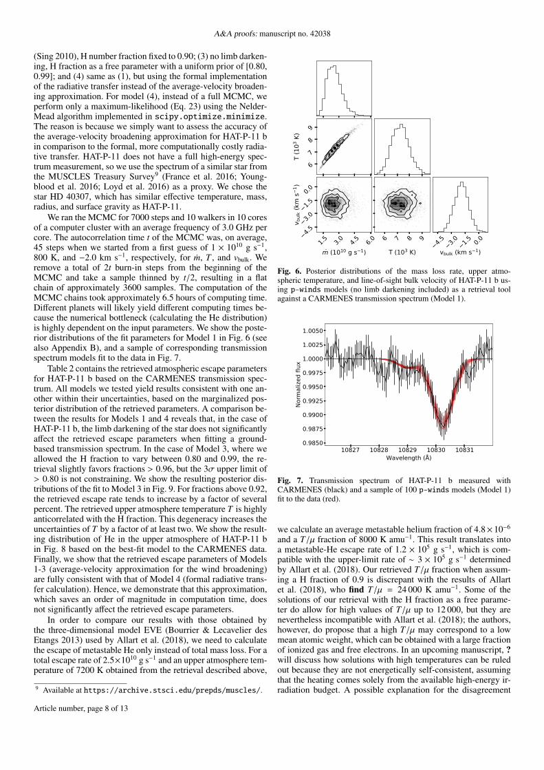
We ran the MCMC for 7000 steps and 10 walkers in 10 coresof a computer cluster with an average frequency of 3.0 GHz percore. The autocorrelation time t of the MCMC was, on average,45 steps when we started from a first guess of 1 × 1010 g s−1,800 K, and −2.0 km s−1, respectively, for m, T , and vbulk. Weremove a total of 2t burn-in steps from the beginning of theMCMC and take a sample thinned by t/2, resulting in a flatchain of approximately 3600 samples. The computation of theMCMC chains took approximately 6.5 hours of computing time.Different planets will likely yield different computing times be-cause the numerical bottleneck (calculating the He distribution)is highly dependent on the input parameters. We show the poste-rior distributions of the fit parameters for Model 1 in Fig. 6 (seealso Appendix B), and a sample of corresponding transmissionspectrum models fit to the data in Fig. 7.

Table 2 contains the retrieved atmospheric escape parametersfor HAT-P-11 b based on the CARMENES transmission spec-trum. All models we tested yield results consistent with one an-other within their uncertainties, based on the marginalized pos-terior distribution of the retrieved parameters. A comparison be-tween the results for Models 1 and 4 reveals that, in the case ofHAT-P-11 b, the limb darkening of the star does not significantlyaffect the retrieved escape parameters when fitting a ground-based transmission spectrum. In the case of Model 3, where weallowed the H fraction to vary between 0.80 and 0.99, the re-trieval slightly favors fractions > 0.96, but the 3σ upper limit of> 0.80 is not constraining. We show the resulting posterior dis-tributions of the fit to Model 3 in Fig. 9. For fractions above 0.92,the retrieved escape rate tends to increase by a factor of severalpercent. The retrieved upper atmosphere temperature T is highlyanticorrelated with the H fraction. This degeneracy increases theuncertainties of T by a factor of at least two. We show the result-ing distribution of He in the upper atmosphere of HAT-P-11 bin Fig. 8 based on the best-fit model to the CARMENES data.Finally, we show that the retrieved escape parameters of Models1-3 (average-velocity approximation for the wind broadening)are fully consistent with that of Model 4 (formal radiative trans-fer calculation). Hence, we demonstrate that this approximation,which saves an order of magnitude in computation time, doesnot significantly affect the retrieved escape parameters.

In order to compare our results with those obtained bythe three-dimensional model EVE (Bourrier & Lecavelier desEtangs 2013) used by Allart et al. (2018), we need to calculatethe escape of metastable He only instead of total mass loss. For atotal escape rate of 2.5×1010 g s−1 and an upper atmosphere tem-perature of 7200 K obtained from the retrieval described above,

9 Available at https://archive.stsci.edu/prepds/muscles/.

6789

T (1

03 K)

1.5 3.0 4.5 6.0

m (1010 g s 1)

4.53.01.50.0

v bul

k (km

s1 )

6 7 8 9

T (103 K)4.5 3.0 1.5 0.0

vbulk (km s 1)

Fig. 6. Posterior distributions of the mass loss rate, upper atmo-spheric temperature, and line-of-sight bulk velocity of HAT-P-11 b us-ing p-winds models (no limb darkening included) as a retrieval toolagainst a CARMENES transmission spectrum (Model 1).

10827 10828 10829 10830 10831Wavelength (Å)

0.9850

0.9875

0.9900

0.9925

0.9950

0.9975

1.0000

1.0025

1.0050

Norm

alize

d flu

x

Fig. 7. Transmission spectrum of HAT-P-11 b measured withCARMENES (black) and a sample of 100 p-winds models (Model 1)fit to the data (red).

we calculate an average metastable helium fraction of 4.8×10−6

and a T/µ fraction of 8000 K amu−1. This result translates intoa metastable-He escape rate of 1.2 × 105 g s−1, which is com-patible with the upper-limit rate of ∼ 3 × 105 g s−1 determinedby Allart et al. (2018). Our retrieved T/µ fraction when assum-ing a H fraction of 0.9 is discrepant with the results of Allartet al. (2018), who find T/µ = 24 000 K amu−1. Some of thesolutions of our retrieval with the H fraction as a free parame-ter do allow for high values of T/µ up to 12 000, but they arenevertheless incompatible with Allart et al. (2018); the authors,however, do propose that a high T/µ may correspond to a lowmean atomic weight, which can be obtained with a large fractionof ionized gas and free electrons. In an upcoming manuscript, ?will discuss how solutions with high temperatures can be ruledout because they are not energetically self-consistent, assumingthat the heating comes solely from the available high-energy ir-radiation budget. A possible explanation for the disagreement


https://archive.stsci.edu/prepds/muscles/


Table 2. Upper atmosphere properties retrieved for HAT-P-11 b from the CARMENES transmission spectrum.

Model m T vbulk H fraction(×1010 g s−1) (×103 K) (km s−1)

1 2.5+0.8−0.6 7.2 ± 0.7 −1.9 ± 0.8 0.90 (fixed)

2 2.3+0.7−0.5 7.2+0.7

−0.6 −1.9 ± 0.8 0.90 (fixed)3 2.6+2.6

−0.8 7.1+1.0−0.9 −1.9 ± 0.8 > 0.80 (3σ)

4 2.1 6.7 −1.9 0.90 (fixed)

2.5 5.0 7.5 10.0 12.5 15.0 17.5 20.0Radius (Rpl)

10 2

100

102

104

106

108

1010

Num

ber d

ensit

y (c

m3 )

HAT-P-11 b, Model 1He singletHe tripletHe ionized

Fig. 8. Distribution of He in the upper atmosphere of HAT-P-11 b basedon the best-fit solution obtained by fitting p-winds models (no limbdarkening included) to the CARMENES transmission spectrum (Model1).

6.07.59.0

10.5

T (1

03 K)

3.01.50.0

v bul

k (km

s1 )

9.9 10.2

10.5

10.8

11.1

log m (g s 1)

0.840.880.920.96

H fra

ctio

n

6.0 7.5 9.0 10.5

T (103 K)3.0 1.5 0.0

vbulk (km s 1)0.8

40.8

80.9

20.9

6H fraction

Fig. 9. Same as Fig. 6, but including the H fraction as a free parameterto be fit (Model 3).

can be due to modeling difference, since Allart et al. (2018) usea hydrostatic model while we use a hydrodynamic one; since ahydrostatic thermosphere is less extended, it needs a higher tem-perature to increase the density of He enough to be detectable athigh altitudes.

The bulk velocity of −1.9 ± 0.8 km s−1 is consistent withthe net blueshift of 3 km s−1 reported by Allart et al. (2018),which was previously interpreted as a high-altitude wind flowing

from the day- to the night-side of the planet. This net blueshiftis not predicted by the one-dimensional Parker wind model,which is the reason for fitting it as a free parameter in our mod-els. More complex, tridimensional models that take into accountother physical processes may be necessary to determine the exactmechanism that causes this bulk velocity shift in the metastableHe absorption signature.

3.2. Escape rate upper limit for a non-detection in GJ 436 b

GJ 436 b is a high-profile case of atmospheric escape becauseit possesses the deepest transmission spectrum feature detectedto date: a repeatable 50% in-transit absorption in Lyman-α (Ku-low et al. 2014; Ehrenreich et al. 2015; Lavie et al. 2017; DosSantos et al. 2019), which is explained by a large volume of ex-ospheric neutral H fed by escape (Bourrier et al. 2016; VillarrealD’Angelo et al. 2021). In fact, Oklopcic & Hirata (2018) pre-dict a metastable He signature as deep as 9% in the core of thestrongest line of the triplet. However, when GJ 436 b was ob-served by CARMENES, the results yielded only a non-detection(Nortmann et al. 2018).

In this section we attempt to measure an upper limit of at-mospheric escape rate to the non-detection of He in GJ 436 band compare it to the result derived from Lyman-α transmis-sion spectroscopy and modeling. The metastable He transmis-sion spectrum of GJ 436 b is rather unfortunately not pub-licly available, but the pipeline-reduced spectral time series fromNortmann et al. (2018) is available in the CARMENES dataarchive10.

We ran an MCMC of 10 000 steps and 10 walkers with threefree parameters: total escape rate, upper atmospheric temper-ature, and the H fraction. We increased the number of stepscompared to the HAT-P-11 b retrieval in order to better explorethe parameter space, since we are expecting to obtain only up-per/lower limits. We did not include limb darkening. Based onprevious theoretical predictions for GJ 436 b (e.g., Salz et al.2016), we set uniform priors of [107, 1012] g s−1 for the massloss and [1 000, 10 000] K for the temperature, and [0.40, 0.99]for the H fraction. We used the high-energy spectrum of GJ 436measured in the MUSCLES Treasury Survey as a source of irra-diation.

The resulting posterior distributions of the free parametersfor GJ 436 b yield, at 99.7% (3σ) confidence, an upper limit of4.5 × 109 g s−1 for the escape rate and a lower limit of 2600 Kfor the upper atmospheric temperature (given the uniform pri-ors above). In broad terms, mass loss rates above this valueor temperatures below the lower limit would yield a detectablemetastable He signature. With the H fraction as a free parame-ter, these 3-σ limits become 3.4 × 1010 g s−1 and 2400 K. Thisresult is consistent with the escape rate of ∼ 2.5 × 108 g s−1 in-ferred by Bourrier et al. (2016), and with the mass loss rate of

10 http://carmenes.cab.inta-csic.es/gto/jsp/nortmannetal2018.jsp


http://carmenes.cab.inta-csic.es/gto/jsp/nortmannetal2018.jsp

http://carmenes.cab.inta-csic.es/gto/jsp/nortmannetal2018.jsp


(6−10)×109 g s−1 inferred by Villarreal D’Angelo et al. (2021),both based on the same Lyman-α transmission spectroscopy dataset.

Given the flat prior of [0.40, 0.99] for the H fraction, the re-sulting posterior distribution of this parameter is not constrain-ing; however, it seems to favor higher values and peaks near 0.99(see Fig. B.3). Interestingly, this result could be seen as an agree-ment with the prediction of a H-rich outflow for GJ 436 b due toselective escape, leading to a He-rich lower atmosphere (Hu et al.2015). We cannot, however, draw strong conclusions on this mat-ter because GJ 436 b had a non-detection of He. More detaileddescriptions that fit both H and He simultaneously in the upperatmosphere of this planet are likely going to yield more defini-tive answers. For example, Lampón et al. (2021) used H den-sities derived from Lyman-α observations to inform metastableHe models, and determine that the warm Neptune GJ 3470 b hasnH/natoms = 0.985+0.010

−0.015.

4. Conclusions

We demonstrate in this manuscript the usage of the open-sourcePython code p-winds to forward model the distribution of Heatoms in the upper atmospheres of exoplanets as well as theircorresponding metastable He transmission spectra of exoplan-ets. The code also enables the retrieval of atmospheric escaperates and temperatures based on observations at high resolutionwhen coupled to an optimization algorithm, such as a maximumlikelihood estimation or an MCMC sampler. A typical retrievaltakes several hours to compute, depending on the setup.

As an implementation of the method originally describedby Oklopcic & Hirata (2018), the forward models produced byp-winds are fully compatible with that study. We also imple-ment changes proposed by Lampón et al. (2020), such as theinclusion of charge exchange of He and H particles. Our imple-mentation includes further improvements, such as the additionof transit geometry and the limb darkening of the host star, aswell as allowing the H fraction (nH/natoms) as a free parameter inthe retrieval.

We used p-winds to fit the escape rate, outflow tempera-ture, and the H fraction of the warm Neptune HAT-P-11 b basedon CARMENES transmission spectroscopy previously reportedin Allart et al. (2018). For a model without limb darkening andwith nH/natoms fixed at 0.90, we find that the escape rate of HAT-P-11 b is (2.5+0.8

−0.6)× 1010 g s−1 and the planetary outflow temper-ature is 7200 ± 700 K. This temperature is in disagreement withthe value of T/µ calculated by Allart et al. (2018), and it is likelycaused by a key difference between our models – theirs containsa hydrostatic thermosphere, while ours is hydrodynamic. Includ-ing limb darkening does not have a significant impact on the re-trieved parameters of HAT-P-11 b. Allowing the H fraction as afree parameter has a stronger impact because it yields an anticor-relation with the retrieved outflow temperature. It also increasesthe uncertainty of the retrieved atmospheric escape rate. We findthat the H fraction is unconstrained, but with a preference forhigher values. These results are in agreement with those of Lam-pón et al. (2020, 2021), although those authors can constrain theH fraction by analyzing He transmission spectra in conjunctionwith H escape using Lyman-α observations.

Finally, we also attempted to fit limits for the escape rate,outflow temperature, and H fraction of GJ 436 b based on a non-detection with the CARMENES spectrograph reported by Nort-mann et al. (2018). We find an upper limit of 3.4 × 1010 g s−1

for the first and a lower limit of 2400 K for the second at 99.7%confidence. Our upper and lower limit determinations show a

preference for high values of nH/natoms, with the posterior dis-tribution peaking near 0.99. These results are fully compatiblewith the escape rate of ∼ 2.5 × 108 g s−1 inferred by Bourrieret al. (2016) based on Lyman-α transmission spectroscopy. Forboth HAT-P-11 b and GJ 436 b, we find a slight preference forhigh values of H in the atomic fraction, which is in line with theresults of Lampón et al. (2020, 2021) for other hot gas giants.

The main limitations of a one-dimensional, isothermalParker wind model are: 1) It does not capture the three-dimensional nature of very extended atmospheres, particularlywhen they have both a thermospheric and an exospheric con-tributions (see the case of WASP-107 b in Allart et al. 2019;?); 2) it does not take into account the variable profile of tem-perature with radial distance from the planet, which is seen inself-consistent models of escape (e.g., Salz et al. 2016; Allan &Vidotto 2019); and 3) it does not self-consistently consider thesources of heating and cooling that control the atmospheric es-cape process. The usefulness of simple models such as p-windslies in an efficient exploration of the parameter space that definesatmospheric escape (scalability) and ease of use (open-source,fully documented code) when more sophisticated models are notyet warranted.

As for the next steps, we aim to improve p-winds by includ-ing the escape of heavier atomic species, such as C, N, O, Mg,Si, and Fe. This will allow us to use the code to predict and in-terpret observations of metals escaping hot gas giants, such asthe signatures reported by Vidal-Madjar et al. (2013) and Singet al. (2019). We shall also add day-to-nightside winds to theatmospheric modeling, similar to Seidel et al. (2020). Anotheravenue to explore p-winds in the future consists in coupling itwith more complex tridimensional hydrodynamic escape mod-els.Acknowledgements. LADS acknowledges the helpful input of A. Wyttenbach,M. Stalport, A. Oklopcic, J. Stürmer, and M. Zechmeister to the developmentof this project. The authors also thank the referee, Manuel López-Puertas, forthe helpful and detailed review. SV is supported by an NSF Graduate ResearchFellowship and the Paul & Daisy Soros Fellowship for New Americans. RAis a Trottier Postdoctoral Fellow and acknowledges support from the TrottierFamily Foundation, and his contribution was supported in part through a grantfrom Fonds de recherche du Québec – Nature et technologies. This research wasenabled by the financial support from the European Research Council (ERC)under the European Union’s Horizon 2020 research and innovation programme(projects: Four Aces grant agreement No 724427; Spice Dune grant agreementNo 947634; ASTROFLOW grant agreement No 817540), and it has been car-ried out in the frame of the National Centre for Competence in Research Plan-etS supported by the Swiss National Science Foundation (SNSF). The p-windscode makes use of the open source software NumPy (Harris et al. 2020), SciPy(Virtanen et al. 2020), Pillow (https://python-pillow.org), and Astropy(Astropy Collaboration et al. 2018). The results of this manuscript were alsomade possible by the open source software Matplotlib (Hunter 2007), Open-MPI (https://www.open-mpi.org), Jupyter (Kluyver et al. 2016), MPI forPython (mpi4py; Dalcin et al. 2011), emcee (Foreman-Mackey et al. 2013), andschwimmbad (Price-Whelan & Foreman-Mackey 2017). Finally, the authors alsoextend a special thanks to the platforms GitHub, Conda-Forge, Read the Docs,and Travis.ci for the valuable support of open-source initiatives.

ReferencesAllan, A. & Vidotto, A. A. 2019, MNRAS, 490, 3760Allart, R., Bourrier, V., Lovis, C., et al. 2019, A&A, 623, A58Allart, R., Bourrier, V., Lovis, C., et al. 2018, Science, 362, 1384Alonso-Floriano, F. J., Snellen, I. A. G., Czesla, S., et al. 2019, A&A, 629, A110Astropy Collaboration, Price-Whelan, A. M., Sipocz, B. M., et al. 2018, AJ, 156,

123Bean, J. L., Raymond, S. N., & Owen, J. E. 2021, Journal of Geophysical Re-

search (Planets), 126, e06639Beaugé, C. & Nesvorný, D. 2013, ApJ, 763, 12Bourrier, V., dos Santos, L. A., Sanz-Forcada, J., et al. 2021, A&A, 650, A73Bourrier, V., Ehrenreich, D., Wheatley, P. J., et al. 2017, A&A, 599, L3


https://python-pillow.org

https://www.open-mpi.org


Bourrier, V. & Lecavelier des Etangs, A. 2013, A&A, 557, A124Bourrier, V., Lecavelier des Etangs, A., Ehrenreich, D., et al. 2018, A&A, 620,

A147Bourrier, V., Lecavelier des Etangs, A., Ehrenreich, D., Tanaka, Y. A., & Vidotto,

A. A. 2016, A&A, 591, A121Carolan, S., Vidotto, A. A., Plavchan, P., Villarreal D’Angelo, C., & Hazra, G.

2020, MNRAS, 498, L53Chaffin, M. S., Chaufray, J. Y., Deighan, J., et al. 2015, Geophys. Res. Lett., 42,

9001Chamberlain, J. W. 1963, Planet. Space Sci., 11, 901Claret, A. 2000, A&A, 363, 1081Claret, A. & Hauschildt, P. H. 2003, A&A, 412, 241Cubillos, P., Erkaev, N. V., Juvan, I., et al. 2017, MNRAS, 466, 1868Dalcin, L. D., Paz, R. R., Kler, P. A., & Cosimo, A. 2011, Advances in Water

Resources, 34, 1124, new Computational Methods and Software ToolsDiaz-Cordoves, J. & Gimenez, A. 1992, A&A, 259, 227Dos Santos, L. A., Bourrier, V., Ehrenreich, D., et al. 2021, A&A, 649, A40Dos Santos, L. A., Ehrenreich, D., Bourrier, V., et al. 2020a, A&A, 640, A29Dos Santos, L. A., Ehrenreich, D., Bourrier, V., et al. 2020b, A&A, 634, L4Dos Santos, L. A., Ehrenreich, D., Bourrier, V., et al. 2019, A&A, 629, A47Ehrenreich, D., Bourrier, V., Wheatley, P. J., et al. 2015, Nature, 522, 459Foreman-Mackey, D., Hogg, D. W., Lang, D., & Goodman, J. 2013, PASP, 125,

306Fossati, L., Haswell, C. A., Froning, C. S., et al. 2010, ApJ, 714, L222France, K., Loyd, R. O. P., Youngblood, A., et al. 2016, ApJ, 820, 89Fulton, B. J. & Petigura, E. A. 2018, AJ, 156, 264Fulton, B. J., Petigura, E. A., Howard, A. W., et al. 2017, AJ, 154, 109Gaidos, E., Hirano, T., Wilson, D. J., et al. 2020, MNRAS, 498, L119García Muñoz, A., Fossati, L., Youngblood, A., et al. 2021, ApJ, 907, L36Hardegree-Ullman, K. K., Zink, J. K., Christiansen, J. L., et al. 2020, ApJS, 247,

28Harris, C. R., Millman, K. J., van der Walt, S. J., et al. 2020, Nature, 585, 357Hu, R., Seager, S., & Yung, Y. L. 2015, ApJ, 807, 8Hunter, J. D. 2007, Computing in Science & Engineering, 9, 90Indriolo, N., Hobbs, L. M., Hinkle, K. H., & McCall, B. J. 2009, ApJ, 703, 2131Jensen, A. G., Redfield, S., Endl, M., et al. 2012, ApJ, 751, 86Kameda, S., Ikezawa, S., Sato, M., et al. 2017, Geophys. Res. Lett., 44, 11,706Kasper, D., Bean, J. L., Oklopcic, A., et al. 2020, AJ, 160, 258King, G. W., Wheatley, P. J., Bourrier, V., & Ehrenreich, D. 2019, MNRAS, 484,

L49Kirk, J., Alam, M. K., López-Morales, M., & Zeng, L. 2020, AJ, 159, 115Klinglesmith, D. A. & Sobieski, S. 1970, AJ, 75, 175Kluyver, T., Ragan-Kelley, B., Pérez, F., et al. 2016, in Positioning and Power

in Academic Publishing: Players, Agents and Agendas, ed. F. Loizides &B. Scmidt (Netherlands: IOS Press), 87–90

Knutson, H. A., Charbonneau, D., Noyes, R. W., Brown, T. M., & Gilliland, R. L.2007, ApJ, 655, 564

Kopal, Z. 1950, Harvard College Observatory Circular, 454, 1Koskinen, T. T., Yelle, R. V., Lavvas, P., & Lewis, N. K. 2010, ApJ, 723, 116Kreidberg, L. 2015, PASP, 127, 1161Kulow, J. R., France, K., Linsky, J., & Loyd, R. O. P. 2014, ApJ, 786, 132Lamers, H. J. G. L. M. & Cassinelli, J. P. 1999, Introduction to Stellar WindsLampón, M., López-Puertas, M., Lara, L. M., et al. 2020, A&A, 636, A13Lampón, M., López-Puertas, M., Sanz-Forcada, J., et al. 2021, A&A, 647, A129Lavie, B., Ehrenreich, D., Bourrier, V., et al. 2017, A&A, 605, L7Lecavelier Des Etangs, A. 2007, A&A, 461, 1185Lecavelier des Etangs, A., Ehrenreich, D., Vidal-Madjar, A., et al. 2010, A&A,

514, A72Loyd, R. O. P., France, K., Youngblood, A., et al. 2016, ApJ, 824, 102MacLeod, M. & Oklopcic, A. 2021, arXiv e-prints, arXiv:2107.07534Mazeh, T., Holczer, T., & Faigler, S. 2016, A&A, 589, A75Morton, D. C. 2000, ApJS, 130, 403Nortmann, L., Pallé, E., Salz, M., et al. 2018, Science, 362, 1388Oklopcic, A. 2019, ApJ, 881, 133Oklopcic, A. & Hirata, C. M. 2018, ApJ, 855, L11Osterbrock, D. E. & Ferland, G. J. 2006, Astrophysics of gaseous nebulae and

active galactic nucleiOwen, J. E. & Wu, Y. 2013, ApJ, 775, 105Paragas, K., Vissapragada, S., Knutson, H. A., et al. 2021, ApJ, 909, L10Parker, E. N. 1958, ApJ, 128, 664Price-Whelan, A. M. & Foreman-Mackey, D. 2017, The Journal of Open Source

Software, 2Salz, M., Czesla, S., Schneider, P. C., & Schmitt, J. H. M. M. 2016, A&A, 586,

A75Seager, S. & Sasselov, D. D. 2000, ApJ, 537, 916Seidel, J. V., Ehrenreich, D., Pino, L., et al. 2020, A&A, 633, A86Sing, D. K. 2010, A&A, 510, A21Sing, D. K., Désert, J. M., Lecavelier Des Etangs, A., et al. 2009, A&A, 505, 891Sing, D. K., Lavvas, P., Ballester, G. E., et al. 2019, AJ, 158, 91Spake, J. J., Sing, D. K., Evans, T. M., et al. 2018, Nature, 557, 68

Tripathi, A., Kratter, K. M., Murray-Clay, R. A., & Krumholz, M. R. 2015, ApJ,808, 173

Vidal-Madjar, A., Huitson, C. M., Bourrier, V., et al. 2013, A&A, 560, A54Vidal-Madjar, A., Lecavelier des Etangs, A., Désert, J.-M., et al. 2003, Nature,

422, 143Villarreal D’Angelo, C., Vidotto, A. A., Esquivel, A., Hazra, G., & Youngblood,

A. 2021, MNRAS, 501, 4383Virtanen, P., Gommers, R., Oliphant, T. E., et al. 2020, Nature Methods, 17, 261Vissapragada, S., Knutson, H. A., Jovanovic, N., et al. 2020, AJ, 159, 278Waalkes, W. C., Berta-Thompson, Z., Bourrier, V., et al. 2019, AJ, 158, 50Wang, L. & Dai, F. 2021a, ApJ, 914, 98Wang, L. & Dai, F. 2021b, ApJ, 914, 99Wyttenbach, A., Ehrenreich, D., Lovis, C., Udry, S., & Pepe, F. 2015, A&A, 577,

A62Wyttenbach, A., Mollière, P., Ehrenreich, D., et al. 2020, A&A, 638, A87Youngblood, A., France, K., Loyd, R. O. P., et al. 2016, ApJ, 824, 101



Appendix A: The flatstar code

The code implemented in flatstar was originally written as apart of the transit module of p-winds. However, we decidedto transform it into a separate package because this implementa-tion can be useful for other astrophysical applications not neces-sarily related to transmission spectroscopy.

The typical usage of flatstar involves setting a grid shape(Nx,Ny) and stellar radius Rs in number of pixels, and option-ally setting a limb-darkening law. The limb-darkening laws cur-rently implemented in the code are: linear, quadratic (Kopal1950), square-root (Diaz-Cordoves & Gimenez 1992), logarith-mic (Klinglesmith & Sobieski 1970), exponential (Claret &Hauschildt 2003), the three-parameter law of Sing et al. (2009),and the four-parameter law of Claret (2000). Finally, the user canalso set a custom limb-darkening law. The star is always centeredto the grid.

In addition, flatstar can add a planetary transit with user-defined planet-to-star ratio, Rp/Rs, transit impact parameter, b,and phase, φ. The first and fourth contact of the transit are de-fined as the phases −0.5 and +0.5, respectively, independent ofb. The y coordinate of the planetary center (yp) in pixel space iscalculated as

yp = (b × Rs) + Ny/2. (A.1)

The x coordinate of the planetary center (xp) is not as straight-forward to calculate, since we define it based on φ and b. Let θbe the angle between the y axis and the vector that connects thecenter of the star and the planet at first contact:

cos θ =b × Rs

Rp + Rs. (A.2)

The distance β from the planet center to the y axis at first contactis given by

β =(Rp + Rs

)sin θ =

(Rp + Rs

) √1 −

(b ×

Rs

Rp + Rs

)2

. (A.3)

Thus, the distance x0 of the planet center from the border of thesimulation at first contact is

x0 = Nx/2 − β. (A.4)

As the planet moves from the first contact to fourth contact, itcovers a distance of 2β. For arbitrary phases between φ = −0.5(first contact) and φ = +0.5 (fourth contact), the distance xp ofthe planet from the border of the simulation is thus

xp = x0 + 2β × (φ + 0.5). (A.5)

This formulation assumes that the arc that the planet follows dur-ing the transit can be approximated to a chord.

The grid can be super-sampled in order to avoid "hard" pixeledges when the grid size is coarse. This is useful to save com-putation time in cases where we need to mass produce gridswhile conserving the precision of intensities (which is the caseof atmospheric retrievals with p-winds). By default, the resam-pling algorithm is the "box" method, which takes the value ofeach pixel with fixed weights to compute the average flux of theresampled pixel. We do not recommend using flatstar to fitwide band photometric light curves, since the computation timeis much longer than other codes that implement analytical equa-tions to calculate light curves, such as batman (Kreidberg 2015).

Appendix B: Other posterior distributions for thefits to HAT-P-11 b and GJ 436 b data

6789

T (1

03 K)

1 2 3 4 5

m (1010 g s 1)

4.53.01.50.0

v bul

k (km

s1 )

6 7 8 9

T (103 K)4.5 3.0 1.5 0.0

vbulk (km s 1)

Fig. B.1. Posterior distribution of parameters of HAT-P-11 b fit to theCARMENES transmission spectrum using a model with a quadraticlimb-darkening law and coefficients c1 = 0.63 and c2 = 0.09.

7.2 7.8 8.4 9.0 9.6

log m (g s 1)

3.04.56.07.59.0

T (1

03 K)

3.0 4.5 6.0 7.5 9.0

T (103 K)

Fig. B.2. Same as Fig. B.1, but for GJ 436 b with the H fraction fixed to0.90 and no limb darkening.



4

6

8

T (1

03 K)

7.2 8.0 8.8 9.6 10.4

log m (g s 1)

0.45

0.60

0.75

0.90

H fra

ctio

n

4 6 8

T (103 K)0.4

50.6

00.7

50.9

0H fraction

Fig. B.3. Same as Fig. B.2, but with the H fraction as a free parameter.


Documents

p-winds: an open-source Python code to model planetary