POVRAY: a tool for scientific visualisation

Paul BourkeWASP, UWA

Introduction

• POVRay is a raytracer. For each position (pixels) in the image plane rays are traced from a virtual camera into a scene. The scene is described by geometry, materials, lighting, atmospherics. The result is an image representing what the virtual camera would “see”.

• Well suited to many visualisation problems where precise/subtle visual cues or high quality imagery is required.

• Large user community. Currently undergoing significant development.

Strengths

• Very powerful scene description language!Human readable.

• High level primitives, not limited to polygonal mesh approximations. (sphere != thousands of triangles)

• Able to handle large data volumes.

• High quality rendering can be achieved.

• Available as source code, modification possible.

• Cross platform: Mac OS-X, MSWindows, Linux .....

• Integrates well with UNIX scripting options.

• Reasonably good documentation and third party online support.

Limitations

• Lack of a good cross platform graphical front end. Important for animators, less important for scientific/data visualisation.

• Not interactive (yet), edit-render-view cycle.

• Limited built-in support for multiple CPUs, no support (yet) for clusters or multiple processors. There are ways of rendering single images or animations in parallel.

• Poor/limited IO handling capabilities => need to write programs that convert data to geometry.

Typical (one possible) Work Flow

• Create a POVRay scene description file, just a text file eg: myscene.pov

• Create a settings file, also a text file with rendering optionseg: myscene.ini

• Render it using the POVRay engine run from the command line (assuming UNIX operating system)eg: povray +imyscene.pov myscene.ini

• View the result in an image viewereg: GIMP, PhotoShop, XV ....

Geometric Primitives

• Solids: sphere, cone (cylinder), box, prism, surface of revolution (lathe), superellipse, torus, text, .... and others.

• Solids: blob, sphere sweep, CSG constructions of solids.

• Surfaces: disc, patch, mesh (mesh2), polygon, triangle, plane (infinite), .... and others.

• Surfaces: isosurface, parametric surface, height field (actually a solid)

Surface Properties: Textures

• pigment: colour/transparency of the surface.

• normal: vector perpendicular to a point on the surface, can be used for bump maps.

• finish: ambient, diffuse, specular reflection coefficients.

• variation across surface supported by maps, patterns, and images.

Camera Model

• Position, view direction, up vector, aperture, aspect ratio

• Left or right handed

• Perspective, orthographic, fisheye, panoramic, spherical, ... and others

Lighting Model

• Ambient light.

• Types: point lights, spot lights, area lights, and others.

• Shadowless lights.

• Light fading with distance.

• Atmospheric, media, fog effects.

• Radiosity.

CSG: Constructive Solid Geometry

• See csg.pov

• Operations: union, intersection, difference, merge.

• Can only be applied to “solid” objects.

difference { sphere { <0,0,0>, 0.5 } sphere { <0.2,0.3,0>, 0.35 } }

union { sphere { <0,0,0>, 0.5 } sphere { <0.2,0.3,0>, 0.35 } }

intersection { sphere { <0,0,0>, 0.5 } sphere { <0.2,0.3,0>, 0.35 } }

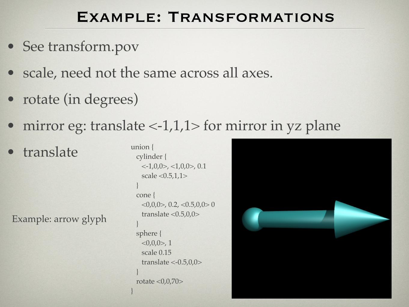
Example: Transformations

• See transform.pov

• scale, need not the same across all axes.

• rotate (in degrees)

• mirror eg: translate <-1,1,1> for mirror in yz plane

• translate union { cylinder { <-1,0,0>, <1,0,0>, 0.1 scale <0.5,1,1> } cone { <0,0,0>, 0.2, <0.5,0,0> 0 translate <0.5,0,0> } sphere { <0,0,0>, 1 scale 0.15 translate <-0.5,0,0> } rotate <0,0,70>}

Example: arrow glyph

Example: calabi-yau surface

• See calabiyau.c and calabiyau.pov

• triangles generated in external C program, #include the result into a scene file.

• More efficient to use a mesh structure.

triangle { <1.18948,0.32963,0.980681>, <1.17523,0.3227,0.960063>, <1.17508,0.339471,0.954446> texture { pigment { color rgbt <0,0,1,TRANSPARENCY> } finish { thefinish } normal { thenormal } }}

union { #include "calabiyau.inc"}

One triangle from many in calabiyau.inc

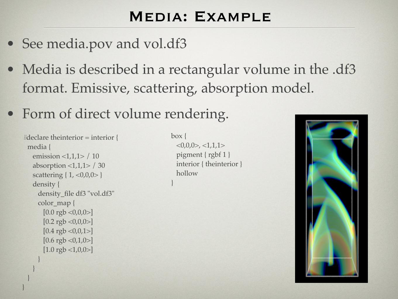
Media: Example

• See media.pov and vol.df3

• Media is described in a rectangular volume in the .df3 format. Emissive, scattering, absorption model.

• Form of direct volume rendering.#declare theinterior = interior { media { emission <1,1,1> / 10 absorption <1,1,1> / 30 scattering { 1, <0,0,0> } density { density_file df3 "vol.df3" color_map { [0.0 rgb <0,0,0>] [0.2 rgb <0,0,0>] [0.4 rgb <0,0,1>] [0.6 rgb <0,1,0>] [1.0 rgb <1,0,0>] } } }}

box { <0,0,0>, <1,1,1> pigment { rgbf 1 } interior { theinterior } hollow}

No Points or Lines!

• See rings.pov and rings.inc

• In general a raytracer cannot trace idealised points or lines, they are infinitely thin so a ray never strikes them.

• Solution: cylinders, cones, and spheres (or sphere sweep).

sphere { <5.4,0.06,0.08>, ringradius}cylinder { <5.4,0,0>, <5.4,0.06,0.08>, ringradius}sphere { <5.4,0,0>, ringradius}

Surfaces: parametric/isosurface

• See isosurface.pov and parametric.pov

• Only functions not volumetric (voxel) data.

parametric { function { cos(2*pi*u - pi/2)*cos(2*pi*(-u+v)+pi/2) } function { cos(2*pi*v - pi/2)*cos(2*pi*(-u+v)+pi/2) } function { cos(2*pi*v - pi/2)*cos(2*pi*u-pi/2) } <0,0>, <0.5,1> contained_by { sphere { <0,0,0>, 2.5 } } accuracy 0.001 max_gradient 10 texture { T_Brass_5C } scale 0.9}

isosurface { function { (pow(x,2)+3) * (pow(y,2)+3) * (pow(z,2)+3) - 32*(x*y*z+1) } contained_by { sphere { <0,0,0>, 2.5} } threshold 0.25 accuracy 0.01 max_gradient 100 open scale 0.8}

Height Field

• See terrain.pov and mars.png

• Surface height represented by image pixel value.

• Very efficient for high surface resolution.

height_field { png "mars.png" smooth pigment { color rgb <0.8,0.8,0.8> } finish { ambient 0.1 diffuse 0.7 specular 0.2 } translate <-0.5,0.0,-0.5> scale <2,0.2,2>}

Programming Language

• Comments: // ... or /* ... */

• #declare, #local

• #include

• #while .. #end loops

• #if ... #else ... #end

• #switch, #case, #range, #break ... #end

• #macro .. #end

• #fopen, #fclose, #fread, #fwrite

• functions, builtin and user defined

Programming Example

• See lorenz.pov

• Creates a macro that iterates to create the attractor.

• Note use of #local rather than #declare

// N: Total number of iterations// h, a, b, c: Parameters describing the attractor// x0, y0, z0: Seed position// rad: Radius of spheres/cylinders#macro lorenz(h, a, b, c, x0, y0, z0, N, rad) : :#end

object { lorenz(0.001,10,28,8.0/3.0,0.1,0.0,0.0,100000,RADIUS) translate -VC rotate <0,0,30>}

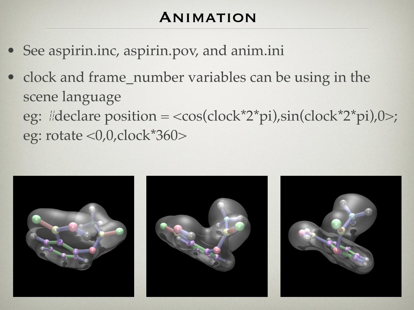
Animation

• See aspirin.inc, aspirin.pov, and anim.ini

• clock and frame_number variables can be using in the scene languageeg: #declare position = <cos(clock*2*pi),sin(clock*2*pi),0>;eg: rotate <0,0,clock*360>

Exercise: MRI, Part 1

• See the “mri” directory.

• mri.df3 is a density file that can be used as media in a box.

• Experiment with the various commented options or create your own visual style.

• Options/considerations:- slicing plane position/angle- colour maps- camera animation- colour map animation- volume sampling precision

Exercise: MRI, Part 2

• Pre-made isosurfaces “*.inc”, or use “polyr” to create your own. See the “createiso” file for details.

• #include multiple isosurfaces with variable transparency.

• See vectors.txt for heat flow data

• Options/considerations:- antialiasing- specular highlight confusion- rendering times

Summary

• Very powerful engine for creating compelling visualisations (Stills and animations). Strengths are high level geometric primitives, realistic shading/lighting model, and the programming aspects of the scene files.

• Lots of online resources: http://povray.org/

• Undergoing continual development.

• Appears to be used increasingly for visualisation especially for applications seeking high visual impact.