Embed Size (px)
Citation preview
8/20/2019 P. Harrison PhD Thesis
http://slidepdf.com/reader/full/p-harrison-phd-thesis 1/141
Image Texture Tools
Texture Synthesis, Texture Transfer,
and Plausible Restoration.
Paul Francis Harrison
Clayton School of Information Technology,
Monash University
2005
1
8/20/2019 P. Harrison PhD Thesis
http://slidepdf.com/reader/full/p-harrison-phd-thesis 2/141
Contents
1 Introduction 9
2 Literature review 15
2.1 Perception of texture . . . . . . . . . . . . . . . . . . . . . 15
2.2 Texture synthesis from a sample . . . . . . . . . . . . . . . 18
2.2.1 Synthesis via perceptual models . . . . . . . . . . . 19
2.2.2 Synthesis via Markov Random Fields . . . . . . . . 21
2.2.3 Texture synthesis on curved surfaces . . . . . . . . 29
2.2.4 Texture transfer . . . . . . . . . . . . . . . . . . . 30
2.3 Plausible image restoration . . . . . . . . . . . . . . . . . 31
2.3.1 Restoration from a texture synthesis perspective . 31
2.3.2 Restoration from a noise removal perspective . . . 32
2.3.3 General image restoration . . . . . . . . . . . . . 36
3 Improving best-fit texture synthesis 38
3.1 Algorithm . . . . . . . . . . . . . . . . . . . . . . . . . . . 39
2
8/20/2019 P. Harrison PhD Thesis
http://slidepdf.com/reader/full/p-harrison-phd-thesis 3/141
CONTENTS 3
3.1.1 Searching the input texture . . . . . . . . . . . . . 40
3.1.2 Refining early-chosen pixel values . . . . . . . . . . 44
3.2 Results . . . . . . . . . . . . . . . . . . . . . . . . . . . . . 45
3.3 Texture transfer . . . . . . . . . . . . . . . . . . . . . . . . 49
3.3.1 Results . . . . . . . . . . . . . . . . . . . . . . . . . 49
3.4 Plausible restoration . . . . . . . . . . . . . . . . . . . . . 53
3.5 Discussion . . . . . . . . . . . . . . . . . . . . . . . . . . . 53
4 Adding best-fit texture synthesis to the GIMP 55
4.1 Discussion . . . . . . . . . . . . . . . . . . . . . . . . . . . 57
5 Patchwork texture synthesis 59
5.1 Method . . . . . . . . . . . . . . . . . . . . . . . . . . . . 60
5.2 Image texture synthesis . . . . . . . . . . . . . . . . . . . . 60
5.2.1 Results . . . . . . . . . . . . . . . . . . . . . . . . . 63
5.2.2 GIMP integration . . . . . . . . . . . . . . . . . . . 65
5.3 Video texture synthesis . . . . . . . . . . . . . . . . . . . . 67
5.3.1 Results . . . . . . . . . . . . . . . . . . . . . . . . . 69
5.4 Texture transfer . . . . . . . . . . . . . . . . . . . . . . . . 70
5.4.1 Results . . . . . . . . . . . . . . . . . . . . . . . . . 71
5.5 Discussion . . . . . . . . . . . . . . . . . . . . . . . . . . . 74

8/20/2019 P. Harrison PhD Thesis
http://slidepdf.com/reader/full/p-harrison-phd-thesis 4/141
CONTENTS 4
6 Plausible restoration of noisy images 76
6.1 Pixel values . . . . . . . . . . . . . . . . . . . . . . . . . . 78
6.2 The texture model . . . . . . . . . . . . . . . . . . . . . . 79
6.3 Minimization algorithm . . . . . . . . . . . . . . . . . . . . 81
6.4 Results . . . . . . . . . . . . . . . . . . . . . . . . . . . . . 82
6.5 A variant for the removal of Gaussian noise . . . . . . . . . 89
6.5.1 Results . . . . . . . . . . . . . . . . . . . . . . . . . 90
6.6 Discussion . . . . . . . . . . . . . . . . . . . . . . . . . . . 93
7 Declarative texture synthesis 95
7.1 Specification of the problem domain . . . . . . . . . . . . . 96
7.1.1 Relation to Markov Random Fields . . . . . . . . . 97
7.2 Literature review . . . . . . . . . . . . . . . . . . . . . . . 98
7.2.1 Tiling patterns . . . . . . . . . . . . . . . . . . . . 98
7.2.2 Procedural texture synthesis . . . . . . . . . . . . . 100
7.3 A tile assembler algorithm . . . . . . . . . . . . . . . . . . 102
7.3.1 Determining if a partial assemblage cannot be com-
pleted . . . . . . . . . . . . . . . . . . . . . . . . . 103
7.3.2 How much to backtrack . . . . . . . . . . . . . . . 103
7.4 Results . . . . . . . . . . . . . . . . . . . . . . . . . . . . . 105
7.4.1 Single-tile patterns . . . . . . . . . . . . . . . . . . 105
8/20/2019 P. Harrison PhD Thesis
http://slidepdf.com/reader/full/p-harrison-phd-thesis 5/141
CONTENTS 5
7.4.2 Further tile sets of interest . . . . . . . . . . . . . . 107
7.4.3 k-morphism and crystallization . . . . . . . . . . . 110
7.5 Relation to cellular automata . . . . . . . . . . . . . . . . 112
7.5.1 Wolfram’s Elementary Cellular Automata . . . . . 112
7.5.2 Causality . . . . . . . . . . . . . . . . . . . . . . . 113
7.6 Discussion . . . . . . . . . . . . . . . . . . . . . . . . . . . 114
8 Conclusion and future work 118
A Test suites 123
A.1 Images . . . . . . . . . . . . . . . . . . . . . . . . . . . . 124
A.2 Texture transfer . . . . . . . . . . . . . . . . . . . . . . . 125
B Paper presented at WSCG-2001 126

8/20/2019 P. Harrison PhD Thesis
http://slidepdf.com/reader/full/p-harrison-phd-thesis 6/141
Abstract
Three image texture operations are identified: synthesis of texture from
a sample, transfer of texture from one image to another, and plausible
restoration of incomplete or noisy images. As human visual perception
is sensitive to details of texture, producing convincing results for these
operations can be hard. This dissertation presents several new methods
for performing these operations. With regard to texture synthesis, this
dissertation presents a variation on the best-fit method [Efros and
Leung, 1999, Garber, 1981] that eliminates the “skew” and “garbage”
effects this method sometimes produces. It is also fast, flexible, and
simple to implement, making it a highly practical method. Also
presented is a simple and fast technique based on random collage. Both
of these techniques can be adapted to transfer texture from one image to
another. Next, a noise removal method that is guided by a model of an
image’s texture, in the form of a non-linear predictor, is presented. The
method is applied to plausibly restoring the texture of images degraded
by compression techniques such as palettization (e.g. GIF), and to the
removal of Gaussian noise, with results comparable to state-of-the-art
wavelet-based methods. Finally, a more abstract form of texture
synthesis is examined, based on the arrangement of tiles of specified
shape. This is used to show the origins of the artifacts seen in best-fit
synthesis.
6
8/20/2019 P. Harrison PhD Thesis
http://slidepdf.com/reader/full/p-harrison-phd-thesis 7/141
Declaration
I, Paul Harrison, declare that this thesis contains no material which has
been accepted for the award of any other degree or diploma in anyuniversity or other institution and to the best of my knowledge contains
no material previously published or written by another person, except
where due reference is made in the text of the thesis.
Paul Harrison
7

8/20/2019 P. Harrison PhD Thesis
http://slidepdf.com/reader/full/p-harrison-phd-thesis 8/141
Acknowledgements
I thank my supervisor, Dr. Alan Dorin, not least for forcing me to learn
how to write. I thank Dr. Peter Tischer for a number of helpfulcriticisms of this work. I also thank the authors of various pieces of free
software—The GIMP, Python, Numeric Python, Latex, and
others—without which this thesis would have been considerably harder
to complete.
8
8/20/2019 P. Harrison PhD Thesis
http://slidepdf.com/reader/full/p-harrison-phd-thesis 9/141
Chapter 1
Introduction
This dissertation describes a number of new tools for working with
texture within the domain of digital images.
It is an easily observed trait that we surround ourselves with texture far
beyond the need of function. Before the modern fashion for austere
perfection, architecture was routinely decorated with intricate patterns
[Fearnley, 1975]. We surround ourselves with interestingly textured
objects and images. Our brains are wired to analyze texture at the
lowest levels of processing (Section 2.1).
There is a gap between our desire for textured objects and the ability of
computer-based design tools to craft texture well. These tools represent
structure using piecewise continuous functions: polygons, spline curves,smooth gradients of colouration, and so on. They therefore afford the
design of smoothly perfect objects over objects who’s design is partly
dictated by the logic of their texture. A “texture” may be applied to the
surface of some designed object, but such texture does not interact with
the structure of the object being designed. Compare this to chiseling
wood or painting a canvas, where the nature of the material influences
the form of the final product.
9
8/20/2019 P. Harrison PhD Thesis
http://slidepdf.com/reader/full/p-harrison-phd-thesis 10/141
Chapter 1 Introduction 10
The word “texture” is peculiar for being applied to many different kinds
of thing. To make any progress, a specific definition is required. The
definition used in this dissertation is that texture is the localized rules of
arrangement of parts that remain consistent throughout an object.
These local rules may give rise to large scale form, but the rules
themselves should refer only to small areas. Mathematically, these rules
may be treated as a Markov Random Field (Section 2.2.2).
This definition allows for complex textures in ways that may not at first
be apparent. A texture by this definition may be composed of a number
of sub-textures, so long as the sub-texture a local area belongs to can be
determined just by looking at that local area. Such a texture will also
have rules for transitions between different sub-textures.1 It is also
possible, and common, for complex large features to emerge from simple
local rules. An example of this is shown on the title page (see
Section 7.4.2).
This definition of texture allows a range of operations, which are usuallyconsidered separate, to be seen as instances of a small number of
operations on textured objects. Three types of operation are examined
in this dissertation:
1. We might synthesize objects of the same texture as a given
object. These creations could inherit desirable properties present
in the original.
2. If we have only part of an object, or if it has been damaged, we
might try to find a plausible restoration of its original form by
reference to its texture. For example, we might try to fill in gaps 2
1This bears some similarity to modulation between keys in music. As in music[Keys, 1961, pp. 99], the exact boundary between two regions may be somewhat fuzzy.
2Filling in of gaps is often referred to as “interpolation”. However interpolation has
a connotation of smoothness, perhaps restoring features such as edges but usually notpreserving any roughness of texture. Such smoothness is actually quite implausible ,
8/20/2019 P. Harrison PhD Thesis
http://slidepdf.com/reader/full/p-harrison-phd-thesis 11/141
Chapter 1 Introduction 11
or correct inaccuracies of measurement, or we might try to infer
the future evolution of a thing changing over time. A restoration is
plausible if it conforms to what is known of the object’s texture.
3. In art, a likeness of an object may be made with a different texture
to the original. This is called texture transfer. For example, an
artist might make a likeness of some object in stone or paint.
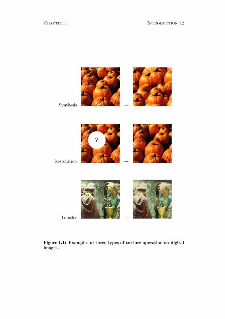
This thesis describes ways to perform these three types of operation on
digital images (see Figure 1.1). The focus is on working with existing
texture (with the exception of Chapter 7, which looks at creating new
textures). For digital images:
1. Synthesis, above, refers to texture synthesis from a sample (not
“procedural” texture synthesis).
2. Plausible restoration, above, refers to techniques for noise removal,
image interpolation, and image in-painting. It also has some
relevance to lossy image compression, in that decompressing a
lossily compressed image requires a plausible guess as to the data
that was discarded.
3. Texture transfer, above, refers to a process of giving an image a
certain texture copied from another image. For example, a
photograph could be given the texture of a painting.
Chapter 2 reviews published literature from this novel viewpoint.
Several apparently disparate problems can be seen as instances of the
texture operations identified above. In particular, the plausible
and readily spotted by eye. Hence the term “plausible restoration” will be used inthis dissertation. Another way of looking at this is to say that interpolation picks that“best possible” restoration, whereas plausible restoration randomly samples from the
field of possibilities.
8/20/2019 P. Harrison PhD Thesis
http://slidepdf.com/reader/full/p-harrison-phd-thesis 12/141
Chapter 1 Introduction 12
Synthesis →
Restoration →
Transfer →
Figure 1.1: Examples of three types of texture operation on digitalimages.
8/20/2019 P. Harrison PhD Thesis
http://slidepdf.com/reader/full/p-harrison-phd-thesis 13/141
Chapter 1 Introduction 13
restoration operation unifies noise removal with interpolation and
in-painting of missing areas.
The current state of the art for texture operations on digital images is
the “best-fit” method and its variants (see Section 2.2.2). The best-fit
method was discovered independently by Garber [1981] and Efros and
Leung [1999]. In its most basic mode of operation, when given a sample
of texture in the form of an image, the best-fit method can synthesize
new samples of that texture. The method may be extended to allow
transfer of texture from one image to another, or to plausibly restore a
missing area of an image by extending surrounding texture into it.
The texture operations are computationally hard problems. The
definition of texture given above allows even for textures that can
perform computation such as cellular automata. Sampling from a
Markov Random Field is in general an NP-hard problem. In practice, we
will see that best-fit synthesis gives rise to types of behavior that,
according to Wolfram [2002], are commonly associated with systemscapable of computation. Synthesis of reasonable generality and quality
most likely requires an algorithm capable of universal computation. This
is discussed further in Chapter 7.
The structure of this dissertation is as follows:
Chapter 2 reviews existing literature on image texture operations.
Chapter 3 describes an improvement to the best-fit method. The best-fit
method has some fundamental problems, which may be reduced though
not removed entirely. Applications to texture synthesis, texture transfer,
and plausible restoration of missing areas are described.
Chapter 4 describes enhancements to existing tools for editing and
manipulating images. Existing image manipulation software such as
“The GIMP” and “Photoshop” have only simple tools for operating on
8/20/2019 P. Harrison PhD Thesis
http://slidepdf.com/reader/full/p-harrison-phd-thesis 14/141
Chapter 1 Introduction 14
texture. In images such as line drawings and diagrams, where the
texture is simple, these tools are adequate. In photographs, or other
images with complex texture, even simple operations require time and
skill to produce a good result. The tool described in this chapter makes
some of these operations easy.
Chapter 5 describes a simpler method of texture synthesis that in some
cases produces results as good as the best-fit method, with less
computation. Its application to texture transfer is also described.
In Chapter 6 it is shown that texture modelling allows the removal of
various kinds of noise, including compression artifacts, from images. A
method is described for plausibly restoring an image in which each pixel
value has some specified degree of uncertainty. It is capable of both noise
removal and interpolation of a missing region, problems usually
considered separate.
Chapter 7 examines some computational aspects of texture synthesis in
the context of the arrangement of shaped tiles, placing certain issues that
arise in preceding chapters into a broader context. The patterns a given
set of tiles may be arranged into are unpredictable and often surprising.
Texture operations on images sit half-way between the fields of Image
Processing and Computer Generated Imagery, and cannot properly be
described as fully belonging to either field. Texture synthesis from a
sample generally requires both modelling and generation of texture.
Texture transfer may be seen as filtering by example, or as a way of
generating new artistic images. Plausible restoration may be seen as
interpolation, but it may also generate new details. Let us begin by
reviewing relevant literature from both of these fields.

8/20/2019 P. Harrison PhD Thesis
http://slidepdf.com/reader/full/p-harrison-phd-thesis 15/141
Chapter 2
Literature review
This chapter reviews published literature relating to how people perceive
texture, and how texture may be synthesized, transferred, or used to
restore images.
2.1 Perception of texture
The three images in Figure 2.1 are 8, 64 and 256 colour versions of the
same scene. There is a clear difference between the 8 and 64 colour
versions, but not between the 64 and 256 colour versions, yet all three
have an easily measured difference in texture, namely the number of
distinct colours.
(a) (b) (c)
Figure 2.1: A scene represented using (a) 8 colours, (b) 64 coloursand (c) 256 colours.
15
8/20/2019 P. Harrison PhD Thesis
http://slidepdf.com/reader/full/p-harrison-phd-thesis 16/141
Chapter 2 Literature review 16
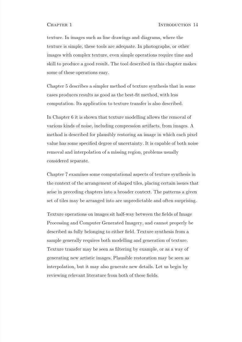
Figure 2.2: Typical figure designed to test texture discrimination[Bergen and Adelson, 1988, Julesz and Krose, 1988].
What is perceived when people look at texture? We do not note every
scratch and mark on every surface, if we did so we would be quickly
overwhelmed. Yet neither are we completely blind to these details.
While not consciously perceiving details, we do perceive what kind of
details there are. What form do these perceptions take?
To determine the aspects of a texture that are perceived, one can test
what textures people can discriminate between. A common method is to
present people with a figure consisting of several different textures, and
ask them to locate the boundaries. A figure typical of the kind used in
this type of research is shown in Figure 2.2 [Bergen and Adelson, 1988,
Julesz and Krose, 1988].
The boundary between the crosses and L’s in Figure 2.2 is immediately
apparent, it “jumps out at you”. This occurs in some texture
discrimination tasks, while others require closer inspection. Texture
discrimination therefore appears to have two distinct modes [Julesz and
Krose, 1988, Bergen and Adelson, 1988]. The first is a fast unconscious
mode, called “pre-attentive” texture discrimination. It can distinguish
between many, but not all, textures. The second mode occurs when we

8/20/2019 P. Harrison PhD Thesis
http://slidepdf.com/reader/full/p-harrison-phd-thesis 17/141
Chapter 2 Literature review 17
scrutinize an image closely and consciously. This mode can distinguish
between many more textures, but takes time and conscious attention.
To study the preattentive mode, Hubel and Wiesel [1962] measured the
firing of neurons in a cat’s visual cortex. They found “simple” neurons
that responded to specific patterns such as lines and edges at a specific
point on the retina (presumably to detect structural features), but also
“complex” neurons that responded to similar patterns anywhere within a
certain region of the retina (thus detecting textural properties). They
propose that these two types of neuron form the early stages of
processing in the visual cortex.
The patterns detected by these neurons do not seem to be
predetermined, but rather form during a “critical period” of
development. For example, Blakemore and Cooper [1970] raised kittens
that were exposed only to lines of a particular orientation during the
critical period. Subsequently the kittens had difficulty perceiving lines of
different orientation.
Bergen and Adelson [1988] propose a “feature pyramid” as a model of
these pattern detecting neurons. A feature pyramid is a collection of
edge and spot detectors of different scales. Feature pyramids build on
the idea of “image pyramids”. The image pyramid of an image is a
sequences of images at different resolutions: the image at full resolution,
the image at one half resolution, the image at one quarter resolution,
and so on. A feature pyramid is the result of taking an image pyramid
and applying several (linear) filters to each image to extract different
types of feature, such as vertical or horizontal edges. The pixels in such
a pyramid will not map exactly to neurons (which will differ from person
to person in any case), but may represent a collection of features similar
to those detected by people. An example of the features that can be
extracted using a feature pyramid is shown in Figure 2.3.

8/20/2019 P. Harrison PhD Thesis
http://slidepdf.com/reader/full/p-harrison-phd-thesis 18/141
Chapter 2 Literature review 18
Figure 2.3: Example of an image pyramid (left), and some featuresthat might be extracted from it: spots contrasting with their sur-roundings, horizontal edges, vertical edges.
However Julesz and Krose [1988] have shown that feature pyramids are
not a perfect model of human perception, by producing a figure in which
people could easily discriminate two textures but feature pyramids could
not. Julesz suggests that similar figures could be produced for any
feature pyramid [Malik and Perona, 1990]. Malik and Perona [1990] note
that feature pyramids based on non-linear filters can be designed that
do not have this limitation.
2.2 Texture synthesis from a sample
This section reviews methods of texture synthesis from a sample. First
methods based on the perception of texture are reviewed, then methods
based on “Markov Random Fields”.
8/20/2019 P. Harrison PhD Thesis
http://slidepdf.com/reader/full/p-harrison-phd-thesis 19/141
Chapter 2 Literature review 19
2.2.1 Synthesis via perceptual models
If all perceived properties of a texture are replicated in another image,
that image will appear to have the same texture as the original (though
it may differ in properties that are not perceived). We might devise some
measure we believe to be an objective criterion of how similar two
textures are, then design a texture synthesis algorithm that will produce
images that exactly match this criterion. This idea has inspired a variety
of texture synthesis methods.
Heeger and Bergen [1995] describe a method of texture synthesis based
upon the feature pyramid model of Bergen and Adelson [1988], using a
“steerable” feature pyramid. A steerable pyramid detects spots and
vertical and horizontal edges. The method creates an image having, at
each level of the feature pyramid, for each of the three types of feature,
the same histogram as that of the sample. The method performs well on
simple textures, such as rough stone or wood, but fails to produce a
convincing result for textures containing complex features, such as
marble or coral, where correlations between features in the pyramid are
important.
DeBonet [1997] describes a method that uses a “Laplacian” image
pyramid. This type of pyramid has only one kind of feature, spots that
contrast with their surroundings. Unlike the method of Heeger and
Bergen [1995], DeBonet’s method uses correspondences between features,in that the synthesis of features at each level of the pyramid is affected
by previously synthesized features at higher levels in the pyramid. It is
better able to synthesize complex textures such as coral than the method
of Heeger and Bergen [1995]. This is partly because the method
reproduces sections of the texture sample verbatim in the output, rather
than because the texture is modelled more accurately.

8/20/2019 P. Harrison PhD Thesis
http://slidepdf.com/reader/full/p-harrison-phd-thesis 20/141
Chapter 2 Literature review 20
S1 S2 C1
C2 C3 C4
E1 E2 E3
T1 T2
N1 N2 N3
Figure 2.4: Results of applying the synthesis method of Portilla andSimoncelli [1999] to the test suite in Appendix A.1.
Portilla and Simoncelli [1999] describe a method of texture synthesis
using complex wavelets. Complex wavelets are a mathematically elegant
variety of steerable feature pyramids. The method synthesizes an output
which has similar distributions of features and similar co-occurrences of
different features to that of the input image. The technique is notable in
that it produces reasonable (though not perfect) results on complex
textures without copying sections of the input image verbatim. Sample
results of this method are shown in Figure 2.4.
While these methods are motivated by theories of perception, their
results are usually visibly synthetic. This would seem to indicate that
our theories of the perception of texture are as yet incomplete. It also
implies that objective criteria derived from such theories are not a good
way to judge the results of a texture synthesis algorithm: for any
criterion we might devise, we can also devise a texture synthesis
algorithm that is near-perfect by that criterion but still fails to entirely

8/20/2019 P. Harrison PhD Thesis
http://slidepdf.com/reader/full/p-harrison-phd-thesis 21/141
Chapter 2 Literature review 21
fool the human eye. Things are not as bad as they might at first seem,
however. At the current level of art, differences between texture
synthesis algorithms can be characterized quite easily in qualitative
terms and, as people all tend to perceive texture in much the same way
(so far as we know), these qualities though difficult to pose
mathematically are likely to be consistent between observers.
2.2.2 Synthesis via Markov Random Fields
Pixel inter-relationships in a texture may be treated mathematically as a
“Markov Random Field” [Winkler, 1995, pp. 209]. The description of
Markov random fields is necessarily abstract, but places many methods
described in the literature within a single framework. The reader is
encouraged to skim the description below, then read it in detail after
looking at the specific applications to texture synthesis given later in this
section.
A digital image is a two-dimensional array of pixels. Each pixel has a
value (an intensity level if the image is gray-scale, or a vector of colour
intensities if it is coloured). If an image is a sample of a particular
texture, each possible assignment of values to pixels has a certain
probability. A probability distribution may be defined over the space of
all possible assignments of values to pixels in an image. This is called a
“random field”.
A Markov Random Field is a random field with a particular property:
Suppose that all but one of the values of an image are known. If the
image is a sample from a Markov Random Field, then the likelihood of
the unknown pixel having a certain value may be determined solely from
the values of a fixed neighbourhood of surrounding pixels. Knowledge of
values beyond this neighbourhood provides no further information.

8/20/2019 P. Harrison PhD Thesis
http://slidepdf.com/reader/full/p-harrison-phd-thesis 22/141
Chapter 2 Literature review 22
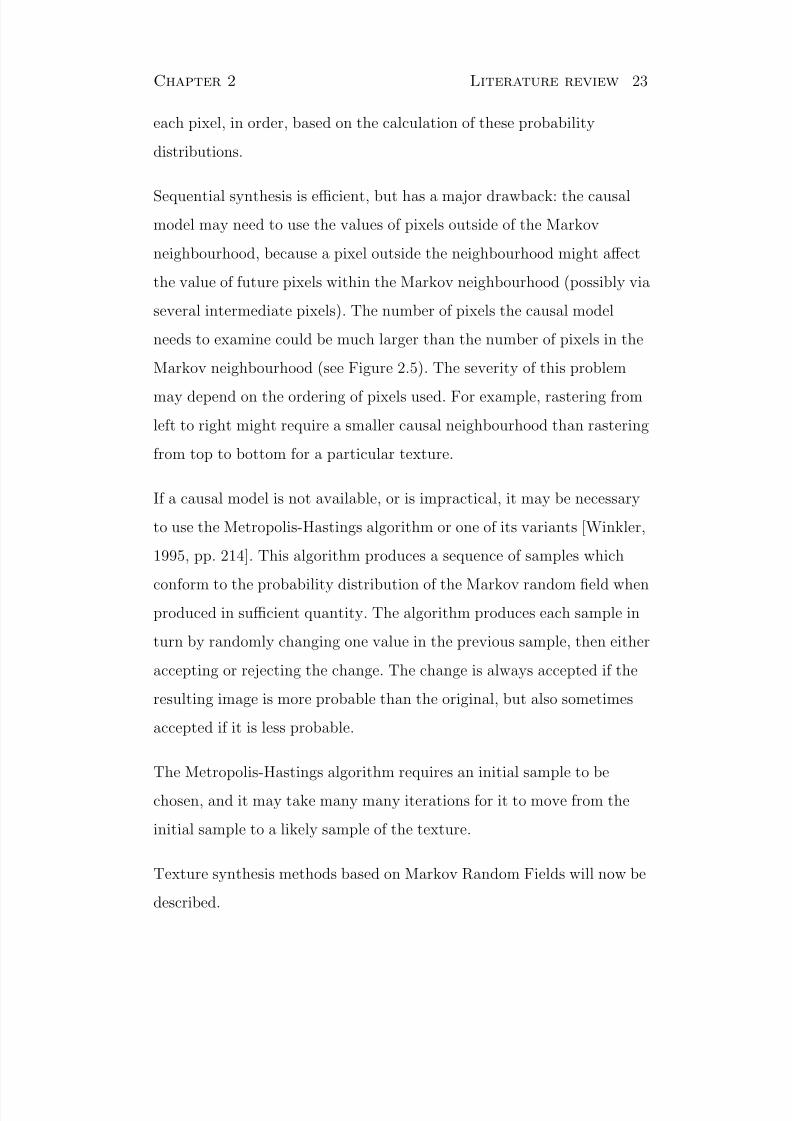
(a) (b)
Figure 2.5: Sequential synthesis: the black dot represents the pixelbeing chosen. (a) A Markov neighbourhood and a neighbourhoodthat might be used by a corresponding causal model are shown. Thecausal neighbourhood includes pixels outside the Markov neighbour-hood. (b) In the worst case, the full width of the image might haveto be used.
Knowledge of the position of the unknown pixel in the image likewise
does not provide further information.
Texture modelling can be seen as the estimation of a Markov Random
Field, and texture synthesis as the production of a sample from a
Markov Random Field.
As pixel values in a Markov Random Field do not depend on the
position in the image, a single sample image is sufficient to estimate a
Markov Random Field model. Every pixel and its neighbours is a sample
from the conditional probability distribution applying to all pixels of the
image.
The method by which a Markov random field is synthesized depends on
the form in which it is specified. Some forms afford fast synthesis, while
others require lengthy computation.
Suppose the pixels of an image are ordered (for example, in raster-scan
order). Further suppose that there is a way to calculate, for each pixel,
the probability distribution of possible values given only preceding pixels
in the ordering (a “causal” model). Then a sample of the texture may be
produced sequentially, one pixel at a time. A random value is chosen for
8/20/2019 P. Harrison PhD Thesis
http://slidepdf.com/reader/full/p-harrison-phd-thesis 23/141
Chapter 2 Literature review 23
each pixel, in order, based on the calculation of these probability
distributions.
Sequential synthesis is efficient, but has a major drawback: the causal
model may need to use the values of pixels outside of the Markov
neighbourhood, because a pixel outside the neighbourhood might affect
the value of future pixels within the Markov neighbourhood (possibly via
several intermediate pixels). The number of pixels the causal model
needs to examine could be much larger than the number of pixels in the
Markov neighbourhood (see Figure 2.5). The severity of this problem
may depend on the ordering of pixels used. For example, rastering from
left to right might require a smaller causal neighbourhood than rastering
from top to bottom for a particular texture.
If a causal model is not available, or is impractical, it may be necessary
to use the Metropolis-Hastings algorithm or one of its variants [Winkler,
1995, pp. 214]. This algorithm produces a sequence of samples which
conform to the probability distribution of the Markov random field whenproduced in sufficient quantity. The algorithm produces each sample in
turn by randomly changing one value in the previous sample, then either
accepting or rejecting the change. The change is always accepted if the
resulting image is more probable than the original, but also sometimes
accepted if it is less probable.
The Metropolis-Hastings algorithm requires an initial sample to be
chosen, and it may take many many iterations for it to move from the
initial sample to a likely sample of the texture.
Texture synthesis methods based on Markov Random Fields will now be
described.

8/20/2019 P. Harrison PhD Thesis
http://slidepdf.com/reader/full/p-harrison-phd-thesis 24/141
Chapter 2 Literature review 24
Methods with distinct modelling and synthesis stages
Chellappa and Kashyap [1985] describe a way to find an invertible linear
filter that produces white noise when applied to a particular sample of
texture. That texture can then be synthesized by applying the inverse of
the filter to white noise. The filter and a description of the distribution
of the white noise values together can be seen as defining a Markov
Random Field. The method can reproduce a range of textures, but the
simplicity of the texture model limits its ability to reproduce complex
textures.
Monne et al. [1981] model texture using a table of the likelihood of each
possible assignment of values occurring in a rectangular block of pixels
at a random position in a textured image. This may be estimated from a
texture sample by counting the number of instances of each possible
block of values. The texture sample must be large enough that enough
instances of each block are present to yield an accurate probability
estimate. The number of estimates required is proportional to the
number of distinct colours in the image raised to the power of the
number of pixels in a block. This will be large if the number of colours
or the size of block is not small, limiting the complexity of textures that
may be modelled.
Monne et al. [1981] synthesize images from this model sequentially line
by line. For each pixel in each line, information from all pixels inpreceding lines is used, as well as preceding pixels in that line (as in
Figure 2.5b). The complexity of this calculation rapidly increases with
the number of colours and number of pixels in a block. It is only
practical with a small block size and a small number of colours.

8/20/2019 P. Harrison PhD Thesis
http://slidepdf.com/reader/full/p-harrison-phd-thesis 25/141
Chapter 2 Literature review 25
Best-fit synthesis
The “best-fit” synthesis method has been independently invented at
least twice [Efros and Leung, 1999, Garber, 1981]. It is an unusual
method in that the new image is synthesized directly from the sample
texture, without an intermediating texture model.
Best-fit is a method of causal synthesis, pixel values are chosen one at a
time. To choose the value of a pixel, neighbouring values in the output
are examined. The sample texture is searched for close matches to this
arrangement of values (hence the name “best-fit”). One of the closest
matches is chosen, and the corresponding pixel’s value is copied to the
output image. The goodness of fit of two neighbourhoods is generally
defined as the sum of squared differences between them.
Sample results of the best-fit method (using Garber’s variant) are shown
in Figure 2.6. These results demonstrate both the strengths of the
best-fit method and its problems. The method produces plausiblevariations on the input, to a level of complexity that no other method of
texture synthesis can match. However, the results tend to be uneven.1
Areas of the input may be copied verbatim, especially if there is only one
example of a certain feature. Sometimes a pattern will repeat itself
inappropriately, producing odd lines or repeating blocks, as can be seen
in C1, C3, and E3. Sometimes the algorithm will simply produce
garbage, as can be seen in E1 and T1. The texture is also skewed, in away that depends on the order in which it was synthesized (in the case
of Figure 2.6, a top-to-bottom left-to-right raster scan).
The obvious culprit for these problems is best-fit synthesis’s causal
nature. The neighbourhood of pixels required to accurately synthesize
1In defense of Garber, it may be possible to tweak his algorithm to reduce thesefaults, perhaps by raising or lowering the amount of randomness involved in pixel
selection—but it is not easy to predict when or how much tweaking will be necessary.

8/20/2019 P. Harrison PhD Thesis
http://slidepdf.com/reader/full/p-harrison-phd-thesis 26/141
Chapter 2 Literature review 26
S1 S2 C1
C2 C3 C4
E1 E2 E3
T1 T2
N1 N2 N3
Figure 2.6: Results of applying the best-fit synthesis method of Gar-ber [1981] to the test suite in Appendix A.1.

8/20/2019 P. Harrison PhD Thesis
http://slidepdf.com/reader/full/p-harrison-phd-thesis 27/141
Chapter 2 Literature review 27
the texture may be large (as in Figure 2.5), however if the
neighbourhood used is large there may be few or no good matches in the
texture sample. The result will either be large sections of the texture
sample copied verbatim to the output, or garbage [Efros and Leung,
1999]. If on the other hand the neighbourhood used is too small, the
output may appear skewed. This effect is especially noticeable if the
image is generated in raster scan order. Efros and Leung [1999] make the
distortion less visible by adding pixels from the center outwards in an
irregular radial pattern. However, it will be seen in Chapters 3 and 7
that this causal nature is not the only source of problems.
The best-fit method is also computationally expensive. For every pixel
in the output image, the entire sample texture must be searched for a
good match. The high dimensionality of the search space means that
even with the use of clever search algorithms, a large proportion of pixels
in the image must be considered.2
A number of variations on the best-fit technique have been devised thatwork around the aforementioned drawbacks [Wei and Levoy, 2000,
Ashikhmin, 2001, Harrison, 2001, Efros and Freeman, 2001, Liang et al.,
2001].
Wei and Levoy [2000] use an image pyramid to reduce the distortion
caused by causal synthesis. The use of a pyramid also represents a way
to efficiently use a large neighbourhood to select pixel values. Output is
generated first at a coarse scale then at progressively finer scales until
the desired scale is reached. In other words, an image pyramid is
generated from the top down. When choosing each pixel value, causal
neighbours on the current level and all neighbours in the next higher
2An odd property of high dimensional spaces is that in a cluster of points eachpoint will be roughly the same distance from all other points. This makes it hard toeliminate groups of distant points en-mass using a “kd-tree” search [Friedman, 1977] or
similar [Yianilos, 1993, Brin, 1995], as might be possible in 2- or 3-dimensional searchproblems.

8/20/2019 P. Harrison PhD Thesis
http://slidepdf.com/reader/full/p-harrison-phd-thesis 28/141
Chapter 2 Literature review 28
level are examined. As the neighbourhoods examined are partly
non-causal, distortion due to sequential synthesis is reduced.
The author [Harrison, 2001] describes a method for ordering the
synthesis of pixels so as to minimize the distortion introduced by causal
synthesis. This method builds the output a pixel at a time, as in the
original best-fit algorithm, but tries at each step to choose a pixel in the
output that is highly constrained by the values of its neighbours, and
therefore, hopefully, who’s causal neighbourhood is not much larger than
its full Markov neighbourhood. This serves to hide the “skew” effect, but
is otherwise not a large improvement on the original best-fit algorithm.
The algorithm is superseded by the best-fit variant described in the next
chapter. A copy of the paper has been relegated to Appendix B.
Efros and Freeman [2001] describe a method they call “image quilting”
which is significantly faster than the best-fit method. In this, the output
is composed of tiles selected from the sample texture. The tiles overlap,
and are selected so that where they overlap they are as similar aspossible. The texture sample is only searched once per tile rather than
once per pixel as in the original best-fit method. A transition line of
minimum discrepancy between adjacent tiles is found, in order to
disguise tile boundaries. Results are comparable to the best-fit method,
except that this method will not produce “garbage”. Liang et al. [2001]
describe a variety of improvements and optimizations to this method.
Kwatra et al. [2003] describe a variant they call “graph-cut” in which the
patches can be of any shape. After initial seeding in the manner of Efros
and Freeman [2001], the edges of patches are allowed to move about
arbitrarily as they search for paths of minimum discrepancy. Graph-cut
can also be used as a tool for producing a seamless boundary between
two images. Xu et al. [2000] found that results acceptable for some
applications may be obtained even if patches are chosen at random, so
long as edges are disguised (either by feathering or best-fit synthesis over

8/20/2019 P. Harrison PhD Thesis
http://slidepdf.com/reader/full/p-harrison-phd-thesis 29/141
Chapter 2 Literature review 29
the border region). They call this random method a “Chaos Mosaic”.
Ashikhmin [2001, 2003] describes an optimization to best-fit synthesis in
which only continuations of the areas copied to surrounding pixels, plus
a small number of random locations, are considered when choosing each
new pixel value. This provides a considerable speed-up, and reduces the
“garbage” effect. It can also reduce quality, since the small number of
candidates considered for each pixel increases the likelihood of there
sometimes being no good match.
2.2.3 Texture synthesis on curved surfaces
In three dimensional computer graphics it is common to want to texture
a curved surface, for example to give an animal realistic skin texture. A
flat texture may be “mapped” over a curved surface, but this usually
distorts the texture—some sections are stretched while others are
compressed. To give a surface an undistorted texture, the texture mustbe synthesized over the surface itself.
If the neighbourhood of a point on a surface can be defined, Markov
Random Field models can be adapted to synthesize texture over
surfaces. Ma and Gagalowicz [1985] describe a way to do this. On a flat
plane, a particular neighbour to a point is a certain distance along a
straight line in a certain direction. On a flat plane, direction may be
defined in terms of an angle from the up vector (vertical axis). On a
curved surface, up and other directions have no clear definition, so a
vector field of up vectors must be specified by hand. On a curved surface
the equivalent of a straight line is a “geodesic”, being the shortest
possible path between two points. So, on a surface, a point’s local
neighbourhood may be specified by stepping along geodesics of set
lengths in directions relative to a given vector field over the surface.

8/20/2019 P. Harrison PhD Thesis
http://slidepdf.com/reader/full/p-harrison-phd-thesis 30/141
Chapter 2 Literature review 30
Turk [2001] and Wei and Levoy [2001] concurrently developed methods
for applying the multi-scale best-fit algorithm of Wei and Levoy [2000] to
surface texture synthesis, both with convincing results. Turk’s method
allows the user to specify direction vectors at a small number of points
on the surface, which are then used to produce a vector field covering the
whole surface, allowing the user to control the direction of the texture.
Praun et al. [2000] describe a simpler method that involves pasting
irregularly shaped patches over the surface until it is covered. This is
similar to the Chaos Mosaic method [Xu et al., 2000]. A vector field is
again required, to choose the orientation of patches. An interesting
finding reported by Praun was that it is better to conform patches to the
vector field than to use one point of the vector field to orient a patch and
minimize distortion of the patch. By conforming closely to the vector
field, stripes of texture curve smoothly rather than bending abruptly at
patch boundaries.
2.2.4 Texture transfer
Texture transfer allows one image to be given the texture of another.
For example, a photograph could be given a paint texture, producing a
synthetic painting. Texture transfer is a natural extension to best-fit
synthesis. During synthesis, pixel values are chosen not just to fit well
with already chosen values but also to conform to features in the targetimage.
Texture transfer via best-fit synthesis was invented independently at
least three times within a short period by the author [Harrison, 2001],
Hertzmann et al. [2001], and Efros and Freeman [2001]. Variants of
best-fit synthesis have also been adapted to texture transfer. Hertzmann
et al. [2001] have adapted the multi-scale method of Wei and Levoy

8/20/2019 P. Harrison PhD Thesis
http://slidepdf.com/reader/full/p-harrison-phd-thesis 31/141
Chapter 2 Literature review 31
[2000], and Efros and Freeman [2001] have adapted their image quilting
method.
Texture transfer can be seen as image filtering by analogy [Hertzmann
et al., 2001]. Image A is to image B as image C is to what image? For
example, texture transfer may be used to sharpen images, given blurred
and sharp versions of some sample image [Hertzmann et al., 2001,
Ashikhmin, 2003].
2.3 Plausible image restoration
Images may be degraded in various ways. A region of an image may be
unavailable (for example, if there is an unwanted object in an image that
must be deleted), or the pixel values of an image may be known only
imprecisely. A degraded image may be plausibly restored by inventing
values for the unknown data that are consistent with what is known.
2.3.1 Restoration from a texture synthesis
perspective
Igehy and Pereira [1997] adapted the texture synthesis method of Heeger
and Bergen [1995] to the task of plausibly filling in missing areas of an
image with homogeneous texture. The texture is matched to the rest of
the image through a border area, such that the grain of the image lines
up with the grain of the synthesized area. This was applied to removing
objects from photographs. For example, an object obscuring a grass
background could be replaced by synthesized grass texture. Drawbacks
of this method are that it can only be used with simple textures, and
that it can not extend features such as edges into the missing region.

8/20/2019 P. Harrison PhD Thesis
http://slidepdf.com/reader/full/p-harrison-phd-thesis 32/141
Chapter 2 Literature review 32
Efros and Leung [1999], in their paper describing the best-fit method,
also describe filling in missing regions of images. This is trivial for the
best-fit method, as it already operates by filling in the image a pixel at a
time. Unlike the method of Igehy and Pereira [1997], this can synthesize
complex textures and extend features such as edges into the missing
region.
As with best-fit texture synthesis, the order in which pixel values are
chosen is important. Criminisi et al. [2003] describe a way to choose a
good order of synthesis so as to best restore edges. Criminisi et al. [2003]
compare their method to the way human visual perception fills in
missing edges of partially occluded objects.
Meyer and Tischer [1998] consider an image with randomly corrupted
pixels (as opposed to a region of missing pixels). A causal Markov model
of the image’s texture is required. This model may derived from similar
but uncorrupted images. The model used has around 1,000 parameters,
and is based on combining the results of several linear predictors. Valuesfor corrupted pixels are then chosen to maximize the likelihood of the
image, given the model. An unusual feature of this method is that it is
stated in terms of image compression – the most likely selection of pixel
values turns out to also be the selection that allows the image to be
stored in the smallest number of bits. The method is also capable of
identifying which pixels are likely to have been corrupted.
2.3.2 Restoration from a noise removal perspective
The removal of additive noise from an image can be seen as a form of
plausible restoration. The addition of noise to an image means that the
pixel values are known only imprecisely, and we may then seek plausible

8/20/2019 P. Harrison PhD Thesis
http://slidepdf.com/reader/full/p-harrison-phd-thesis 33/141
Chapter 2 Literature review 33
true values of the pixels. Many methods of additive noise removal have
been proposed. These methods are of the “interpolation” type (see
footnote in Chapter 1) and seek the best possible restoration, even if this
best restoration is not representative of the full field of plausible
restorations. For example, the restoration will commonly be smoother
than is plausible.
Noise removal is a very large field, and this section represents only a
sampling of existing work sufficient to convey its character.
One straightforward approach is linear filtering. This method derives
from stating that elements in the Fourier transforms of the image
(signal) and the uncertainty about the image (noise) will have Gaussian
distribution. These elements’s variances (the expected “spectral
density”) are estimated, and from these an optimal “Weiner Smoothing
Filter” is derived [Helstrom, 1990]. This filter is always linear. The noise
component is commonly taken to be white noise, having a uniform
spectral density. The image may be estimated to not contain highfrequencies (i.e. to be smooth). Alternatively the spectral density of the
image may be estimated from the spectrum of the noisy image. In either
case, the resulting Weiner Filter will generally be a low-pass filter.
A low-pass filter will blur any sharp edges in an image, so linear filtering
is of limited use for additive noise. The limitations of linear filtering led
to investigation of non-linear filters.
Non-linear approaches described in the literature vary in complexity.
The Lee Filter [Lee, 1980] is an example of a simple but effective
non-linear filter. Where a local estimate of the variance of pixel values is
low the filter blurs the image, but where it is high the image is left
unchanged. Edges, containing a mixture of two levels and thus having
high overall variance, are left un-blurred.

8/20/2019 P. Harrison PhD Thesis
http://slidepdf.com/reader/full/p-harrison-phd-thesis 34/141
Chapter 2 Literature review 34
A more sophisticated method based on minimizing the “Total Variation”
was developed for the US military [Rudin et al., 1992]. The Total
Variation method models the texture of the image as tending to have
small gradient at each point. The magnitude of the gradient is assumed
to have an exponential distribution. Noise is modelled as being
Gaussian. Finding the most likely true image under these assumptions
requires minimizing a norm similar to L1 subject to the constraint that
the noise removed has an a priori specified variance.3
The texture model of the Total Variation method, by using an L1-like
norm, rates smooth gradients and sharp edges as being equally likely.
Consequently, the Total Variation method preserves sharp edges in an
image. A texture model that made a more traditional assumption of a
Gaussian distribution of gradients would prefer smooth gradients to
sharp edges. Rudin et al. [1992] report that the Total Variation method
is superior to the human eye at extracting features from a noisy image.
The current state of the art (to the author’s knowledge) is a method byPortilla et al. [2003].4 This is a complex method, but the results justify
this complexity. The image first is decomposed into a highly-redundant
steerable image pyramid. Elements in this pyramid are then modelled as
being linearly related to their neighbouring elements both in value and
in level of variance. From this model, the average expected value of each
element in the pyramid is computed. An image is then reconstructed
3The L p norm of a list of values xi is (
i |x| p)1
p . A norm L p may be mapped bya monotonically decreasing function to a corresponding probability density function of
form ae(b
i|x|p) (where a and b are constants). For example, L2 may be mapped to a
Gaussian distribution. Minimizing a norm will maximize the corresponding probabilitydensity.
4Two of the authors of this paper previously published a method of texture synthesismotivated by a model of human vision [Portilla and Simoncelli, 1999]. Their work thussomewhat parallels this thesis in considering texture synthesis and noise removal asrelated problems. Broadly, the difference in approaches is that they treat texture asbeing composed of inter-related features whereas this thesis treats texture as the inter-relation of pixels and does not explicitly model features (instead letting features emerge
from the rules of pixel relationships).

8/20/2019 P. Harrison PhD Thesis
http://slidepdf.com/reader/full/p-harrison-phd-thesis 35/141
Chapter 2 Literature review 35
from this de-noised pyramid.
Specialized methods have also been designed to remove the noise
introduced by JPEG compression [Zakhor, 1992, Yang et al., 1993,
Llados-Bernaus et al., 1998, Meier, 1999]. JPEG breaks an image into
8 × 8 pixel blocks and performs a Discrete Cosine Transform on each
block. The output of the transform is quantized and stored concisely.
When decoding JPEG images, there is uncertainty as to the true value
of each element in the block transforms due to quantization. JPEG
decoders assume that each element is independent, and for each element
minimize the expected error by choosing the center of the range of
possible values. This is a reasonable assumption, as the purpose of the
DCT is to decorrelate each 8 × 8 block. However the DCT ignores
correlations between adjacent blocks, and the decoder may produce
visible block borders if the quantization level is too high.
The method of Llados-Bernaus et al. [1998] is typical of JPEG
restoration methods. As in the Total Variation method, this methodminimizes a norm subject to constraints. The image is taken to be more
likely to be smooth than rough, including across block boundaries.
Therefore, differences between neighbouring pixels are expected to be
small. Penalties are imposed on each difference by the use of a “Huber
function”, and these penalties are added to give a measure of how
unlikely a particular reconstruction is. Huber functions are a compromise
between the L2 and L1 norms, combining the smoothness of L2 with the
robustness of L1. They correspond to a Gaussian distribution of values
with fat tails.5 The pixel values are constrained such that the DCT
transform elements, when quantized, match the file being decoded.
Though some of these methods use texture models of moderate
complexity, any non-linear components are specified a priori. Adaptation
5But see Section 3.1.1.
8/20/2019 P. Harrison PhD Thesis
http://slidepdf.com/reader/full/p-harrison-phd-thesis 36/141
Chapter 2 Literature review 36
to the image’s texture, though perhaps embedded in a non-linear
framework, is limited to linear modelling or the tweaking of a small
number of parameters. This limits these methods’s ability to restore
images with novel features.
New procedures for noise removal are constantly being published. Most
of these procedures boil down to ever more elaborate a priori models of
image and noise texture (though they are not necessarily described as
such). Recent papers have included a procedure that constrains the
Total Variation to be below a specified level rather than simply
minimizing it as far as possible [Combettes, 2004], a method for
enhancing edges while blurring other areas based on diffusion processes
[Gilboa et al., 2002], and a denoising technique adapted from fractal
image compression [Ghazel et al., 2003] (a potentially interesting
approach, however the particular iterated function used introduces block
artifacts when used for denoising).
2.3.3 General image restoration
Drori et al. [2003] present an elegant formulation of the plausible
restoration problem. The input is an image where each pixel has an
alpha value in addition to a colour. Pixels with high alpha are known to
high accuracy, while pixels with low alpha are known to low accuracy.
The problem is to find an image such that if the input isalpha-composited over it the result has consistent texture. Though not
stated in the paper, this formulation encompasses the problem of noise
removal if the input image is given a constant alpha value of slightly less
than one.
The solution to this problem presented by Drori et al. [2003] is effective
but inelegantly complicated, combining smooth interpolation, image

8/20/2019 P. Harrison PhD Thesis
http://slidepdf.com/reader/full/p-harrison-phd-thesis 37/141
Chapter 2 Literature review 37
pyramids, and a patch-based variant of the best-fit method. Finding an
elegant solution to this elegantly general problem is an open and
interesting problem.
8/20/2019 P. Harrison PhD Thesis
http://slidepdf.com/reader/full/p-harrison-phd-thesis 38/141
Chapter 3
Improving best-fit texture
synthesis
In the previous chapter, we saw that the best-fit method can be used to
synthesize complex textures, but also that it has some serious problems:
• Speed: Production of each pixel in the output requires a full
search of the input.
• Artifacts: The method sometimes produces “garbage” and
repeated patches.
• Skew: The order in which pixels are chosen can visibly distort the
output.
A long list of attempts to reduce these problems was given in the
previous chapter. These involved the used of multi-scalar synthesis, or
working with blocks of pixels rather than individual pixels. Use of these
techniques places constraints on the size and shape of the image that can
be synthesized. These methods may also introduce artifacts of their own.
For example, in block based synthesis the seam between blocks can
become visible.
38

8/20/2019 P. Harrison PhD Thesis
http://slidepdf.com/reader/full/p-harrison-phd-thesis 39/141
Chapter 3 Improving best-fit texture synthesis 39
10% ... 25% ... 75% ... 100%
Figure 3.1: Pixel values are chosen in random order.
This chapter adds another method to the list.1 The new method is
distinguished, however, by its combination of simplicity, speed, small
number of parameters, and the absence of any constraints on the size and
shape of the area to be synthesized. It is a practical algorithm and is in
current use in the form of an open-source GIMP plug-in (see Chapter 4).
3.1 Algorithm
In this new algorithm, pixel values are chosen one at a time in random
order (as illustrated in Figure 3.1). This avoids any possibility of
consistent skew due to the order in which pixels are selected. When
choosing the value of a pixel, the n nearest pixels that already have
values are located.2 The input image is searched for a good match to the
pattern these pixels form (see next section). Once a good match is
found, the appropriate pixel value is copied from the input texture to the
output. To increase quality, some earlier chosen pixel values are
re-chosen after later pixel values have been chosen (see Section 3.1.2).
Early in the process, when the density of chosen pixels is low, pixel
values will necessarily be chosen on the basis of far distant pixels. Later,
when more of the image has been filled, pixel values are chosen on the
1An earlier attempt at addressing some of these problems was presented as a paperat WSCG’01 [Harrison, 2001], a copy of which is given in Appendix B.
2Or if there are less than n pixels, however many are available. The first pixel iseffectively chosen at random.

8/20/2019 P. Harrison PhD Thesis
http://slidepdf.com/reader/full/p-harrison-phd-thesis 40/141
Chapter 3 Improving best-fit texture synthesis 40
basis of close neighbours. This approach is therefore implicitly (rather
than explicitly ) multi-scalar.
This implicit multi-scalar approach does not constrain the output to be
of a particular set of sizes (as do methods based feature pyramids or
tiles), giving it the flexibility needed for practical applications. The lack
of constraints is of particular importance when performing plausible
restoration of an irregularly shaped area in an image (for example, to
remove an unwanted object or blemish).
3.1.1 Searching the input texture
When choosing each pixel value, only a small number of locations in the
input texture are examined, yielding a considerable speed-up as
compared to a search of the whole image. This optimization was first
introduced by Ashikhmin [2001]. The locations examined are:
• Continuations of the regions in the input texture associated with
the n nearest pixel values that have already been chosen (i.e. as if
the current pixel and one its neighbours formed part of a patch
copied exactly from the input texture).
• A further m random locations.
The use of continuations allows production of good results even when a
small number of locations are examined in each individual search.
The best fit out of each of these locations is selected, based on
comparison of the pattern formed by the n nearest known neighbours of
the current pixel to the pattern formed by pixels at corresponding offsets
about each candidate location. To make this comparison the algorithm

8/20/2019 P. Harrison PhD Thesis
http://slidepdf.com/reader/full/p-harrison-phd-thesis 41/141
Chapter 3 Improving best-fit texture synthesis 41
uses a robust metric3 based on the Cauchy distribution, as described by
[Sebe et al., 2000]. The explanation of this metric first requires
discussion of some background assumptions commonly taken for granted:
Each pattern may be represented by a vector u of values u1 . . . uN , those
values being the colour components (red, green, blue) of each pixel in the
pattern. Let us model the field of all possible patterns as a mixture of
classes (a “mixture model”). We could aggregate sets of similar patterns
in the input into similar classes, but this would throw away information
about individual patterns, producing poor results (see Wei and Levoy
[2000] for example). Instead we shall say that each pattern in the input
represents a single class.
Having only one instance u of each class, the best estimate we can make
of the center of that class is just that instance u. To fully define each
class, we also need a density function giving the spread of possible values
v around that center point u, F (v − u). Let us assume that F is the
same for each class (having only one instance of each class, we have noinformation about spread for individual classes). Let us further assume,
for simplicity, that each dimension of the spread is independent of each
other dimension, and is identically distributed, such that F may be
calculated from a single-dimensional spread function f :
F (x) =N
i=1
f (xi) (3.1)
Now, given a pattern v, we can calculate the likelihood of it having
occurred if it were it an instance of each of these classes by evaluating
F (v − u). If we say that each class is equally likely to occur, the class
producing the greatest F (v − u) will also be the class it is most likely to
3The word “metric” is here used to mean simply a standard way of measuringsomething, and not in the strict mathematical sense of a distance function used todefine a metric space.
8/20/2019 P. Harrison PhD Thesis
http://slidepdf.com/reader/full/p-harrison-phd-thesis 42/141
Chapter 3 Improving best-fit texture synthesis 42
be an instance of, the “best fit”.
To avoid floating-point underflow and in order to simplify calculation
somewhat it is better to work with negative logarithms than raw
probability densities:
− log F (x) =N i=1
− log f (xi) (3.2)
The class that minimizes − log F (v − u) is the best fit. All that remains
is to choose f .
The standard distribution f used in the best-fit algorithm (and in many
other algorithms) is the Gaussian distribution. The Gaussian
distribution is:
1
σ√
2πe−x
2
2σ2 (3.3)
The negative logarithm of this distribution is proportional to x2. This is
the derivation of the commonly used “sum of squares” criterion, also
called the Euclidean distance metric or L2. Note that the same class will
be judged most likely regardless of σ.
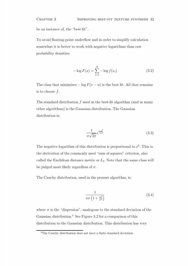
The Cauchy distribution, used in the present algorithm, is:
1
πσ
1 + x2
σ2
(3.4)
where σ is the “dispersion”, analogous to the standard deviation of the
Gaussian distribution.4 See Figure 3.2 for a comparison of this
distribution to the Gaussian distribution. This distribution has very
4
The Cauchy distribution does not have a finite standard deviation.

8/20/2019 P. Harrison PhD Thesis
http://slidepdf.com/reader/full/p-harrison-phd-thesis 43/141
Chapter 3 Improving best-fit texture synthesis 43
Figure 3.2: The Gaussian and Cauchy distributions.
much fatter tails than the Gaussian distribution, making it robust to
outliers. The negative logarithm of this distribution is proportional to:
log
1 + x2
σ2
(3.5)
A sum of these terms is used as the goodness-of-fit metric in the present
algorithm, with one term for each colour component (red, green, blue) of
each pixel compared. σ is significant for this distribution, and must be
specified as a parameter.5
If a Cauchy based metric is used, one or two bad pixels in an otherwise
good match will not cause that match to be rejected outright, as they
would were the Gaussian based metric used. This means that in every
search there will be more matches of comparable merit. Repetition and
“garbage” are reduced, and overall quality is increased. This is
illustrated in Figure 3.4.6
5So long as we are only concerned with finding the most likely match, not relative
likelihoods, the Euclidean distance metric may be simulated in this metric by choosinga very large σ. Indeed, any member of the “t” family of distributions may be sosimulated.
6The predecessor of this current algorithm, described in Harrison [2001], used theabsolute value metric (aka Manhattan distance or L1). This is another robust metric,and derives from the Laplace distribution (e−|x|). This too is more robust than theGaussian derived metric, increasing only linearly with the degree of discrepancy, butis not nearly as robust as the Cauchy derived metric, which increases as the log of the discrepancy. Another reason to favour the Cauchy distribution over the Laplacedistribution is that, as with the Gaussian distribution, it is a member of the Levy alpha-stable family of distributions (see Mandelbrot [1983, pp.368]). These distributions areproduced, amongst other things, in “Levy flights”, a form of random walk commonly
seen in nature (and even stock-market fluctuations [Mandelbrot, 1983, pp.337–340]).Processes that give rise to interesting texture, such as textures with a fractal character,

8/20/2019 P. Harrison PhD Thesis
http://slidepdf.com/reader/full/p-harrison-phd-thesis 44/141
Chapter 3 Improving best-fit texture synthesis 44
3.1.2 Refining early-chosen pixel values
Early-chosen pixel values are chosen on the basis of far-distant pixels,
and may turn out to be inappropriate once nearer pixels have been filled
in. Early chosen pixel values are also not chosen with the benefit of
being able to continue the regions in the input texture associated with
well chosen nearby pixels. For these reasons, the algorithm re-chooses
early chosen pixel values once later pixel values have been chosen.
The sequence of choosing and re-choosing used (where N is the number
of pixels in the output, and p is some constant 0 ≤ p < 1) is this:
Choose the first pixel.
. . .
Choose the first p3N pixels.
Choose the first p2N pixels.
Choose the first pN pixels.
Choose all N pixels.
This sequence allows refinement both in the coarse early stages and the
fine later stages. It makes good use of the ability of well fitting regions
to propagate between neighbouring pixels. The cost of re-choosing can
be offset by examining less locations within each individual search.
Small modifications to the value of p, so long as a corresponding
adjustment is made to n
, have very little affect. When re-choosing, theresult from the earlier search (the pixel’s “continuation of itself”) is
included in the list of locations examined, and therefore not lost. The
value of p used to produce the results presented here was 0.75.
often involve Levy flights.

8/20/2019 P. Harrison PhD Thesis
http://slidepdf.com/reader/full/p-harrison-phd-thesis 45/141
Chapter 3 Improving best-fit texture synthesis 45
3.2 Results
Figure 3.3 shows the result of applying the method to the test suite of
textures given in Appendix A.1. The n = 30 nearest pixels, and m = 80
further random locations were used in the searches. σ = 30 was used in
the goodness-of-fit metric (the range of each colour component being 0
to 255).
There are some flaws in the images produced. Certain features in C1
have been duplicated in an obvious way. C3 appears normal at first
glance, but closer inspection reveals a number of deformed pumpkins (it
is hard to imagine an algorithm that would correctly infer from a single
image that pumpkins are distinct objects). In C4, the cracks do not all
join up as they do in the original. The tiling patterns (T1, T2) did not
produce tiled results. However, overall results were quite faithful to the
input.
As might be expected, the images that were not homogeneous texturesdid not produce sensible results (N1, N2, N3).
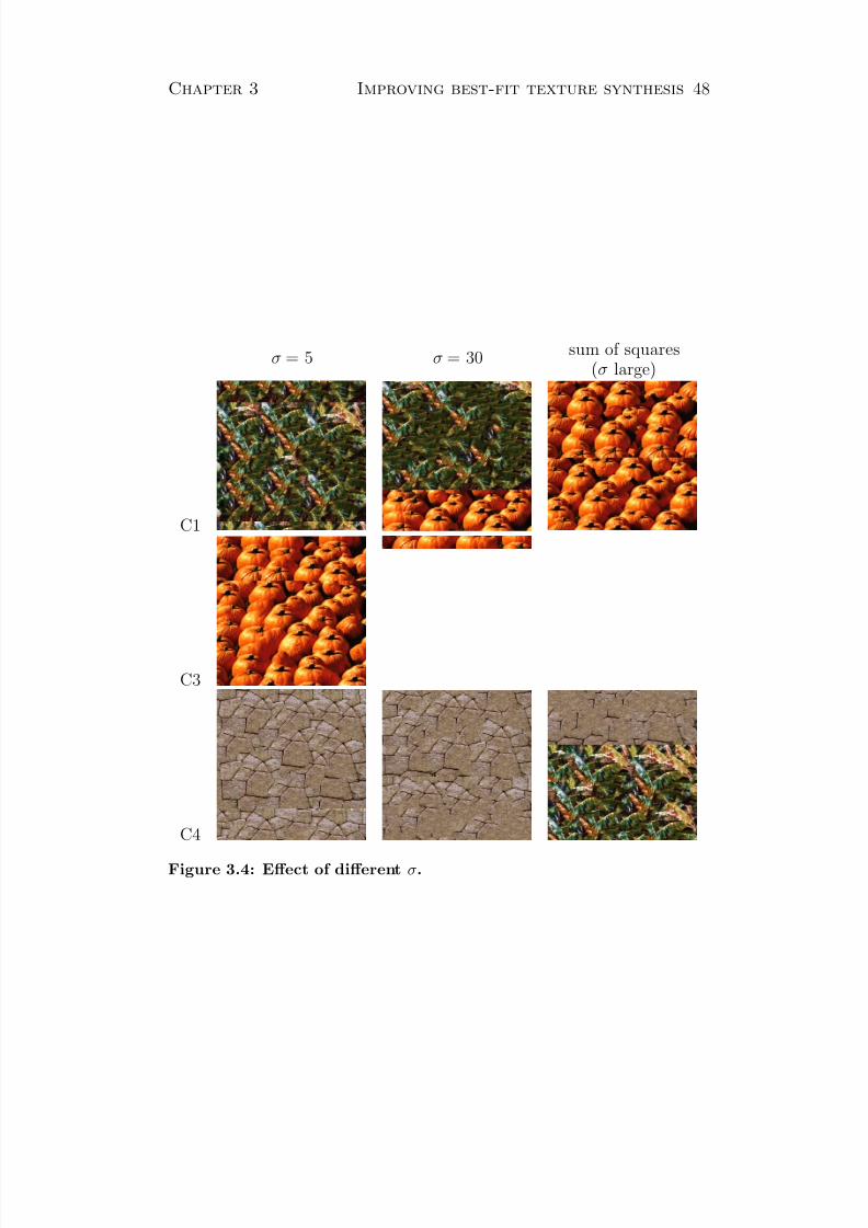
The effect of changing σ is illustrated in Figure 3.4. Small σ produces a
more representative sample of the input texture, but also produces sharp
transitions between patches of texture. Large σ (equivalent to using a
sum-of-squares metric) produces smooth transitions between patches of
texture, but sometimes some features of the texture are over-represented
while others are under-represented. This is akin to the “garbage”
produced by the standard best-fit algorithm (see Figure 2.6).
Each image took around 20 seconds to produce, using a 3GHz Pentium-4
processor. The algorithmic complexity is linear in the size of the output.
Importantly, it is not dependant on the size of the input texture, making
this a suitable algorithm for large texture images. This speed makes it
suitable for interactive use as a smart selection-eraser, useful for

8/20/2019 P. Harrison PhD Thesis
http://slidepdf.com/reader/full/p-harrison-phd-thesis 46/141
Chapter 3 Improving best-fit texture synthesis 46
touching up photographs (this will be discussed further in the next
chapter). It would not be suitable for real-time applications such as
graphics in a computer game. The speed is comparable with that of tile
based methods [Efros and Freeman, 2001, Liang et al., 2001], and the
graph-cut method [Kwatra et al., 2003]. The original best-fit method
[Efros and Leung, 1999, Garber, 1981] is considerably slower, and would
take many minutes to a produce an image of the same size as those
presented here. Ashikhmin [2001], who uses a similar search strategy,
reports a speed considerably faster than that of this method. This is
most likely due to use of a smaller neighbourhood of pixels and less
searching per pixel. Note also that Ashikhmin [2001]’s method produces
visible artifacts due to the raster-scan order in which pixels are chosen.

8/20/2019 P. Harrison PhD Thesis
http://slidepdf.com/reader/full/p-harrison-phd-thesis 47/141
Chapter 3 Improving best-fit texture synthesis 47
S1 S2 C1
C2 C3 C4
E1 E2 E3
T1 T2
N1 N2 N3
Figure 3.3: Texture synthesis results.
8/20/2019 P. Harrison PhD Thesis
http://slidepdf.com/reader/full/p-harrison-phd-thesis 48/141
Chapter 3 Improving best-fit texture synthesis 48
σ = 5 σ = 30 sum of squares(σ large)
C1
C3
C4
Figure 3.4: Effect of different σ.

8/20/2019 P. Harrison PhD Thesis
http://slidepdf.com/reader/full/p-harrison-phd-thesis 49/141
Chapter 3 Improving best-fit texture synthesis 49
3.3 Texture transfer
Texture transfer allows the texture of one image to be transferred to
another (see Section 2.2.4). To perform texture transfer, terms may be
added to the goodness-of-fit metric in order to specify the layout of
different regions of texture in the output image. Two extra images are
required, one being a map of regions in the input and the other a
corresponding map of regions in the output. In these maps, different
colours indicate different regions, and similar colours similar regions. It
sometimes suffices simply to use the images themselves as these maps.
In order to retain the multi-scalar nature of the algorithm, it was
decided to compare these maps at the same locations as the pixel values
being compared, plus the central location. A Gaussian based (squared
difference) rather than Cauchy based goodness-of-fit metric was used for
these terms, as this was found to give better results. Such a metric
heavily penalizes large deviations from the map, while allowing small
deviations. This is a good complement to the Cauchy based metric used
for the texture itself, which heavily penalizes small magnitude deviations
but is proportionately more forgiving of large deviations. The result is
an image that replicates the texture accurately in fine detail, but also
never deviates excessively from the specified output map.
3.3.1 Results
Texture transfer was applied to the texture transfer test suite given in
Appendix A.2, using the texture as its own map. Results are shown in
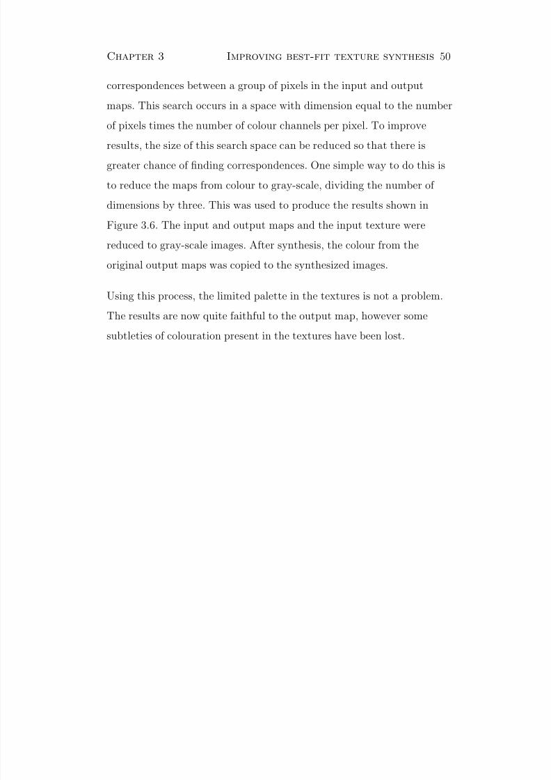
Figure 3.5. Acceptable results were produced from the paint texture
(S1), but the jellybean texture (S2) produced less impressive results.
When selecting pixels, the synthesis procedure is searching for
8/20/2019 P. Harrison PhD Thesis
http://slidepdf.com/reader/full/p-harrison-phd-thesis 50/141
Chapter 3 Improving best-fit texture synthesis 50
correspondences between a group of pixels in the input and output
maps. This search occurs in a space with dimension equal to the number
of pixels times the number of colour channels per pixel. To improve
results, the size of this search space can be reduced so that there is
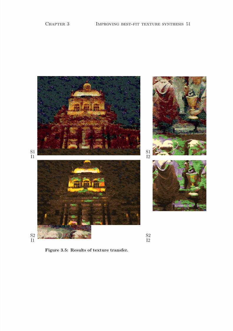
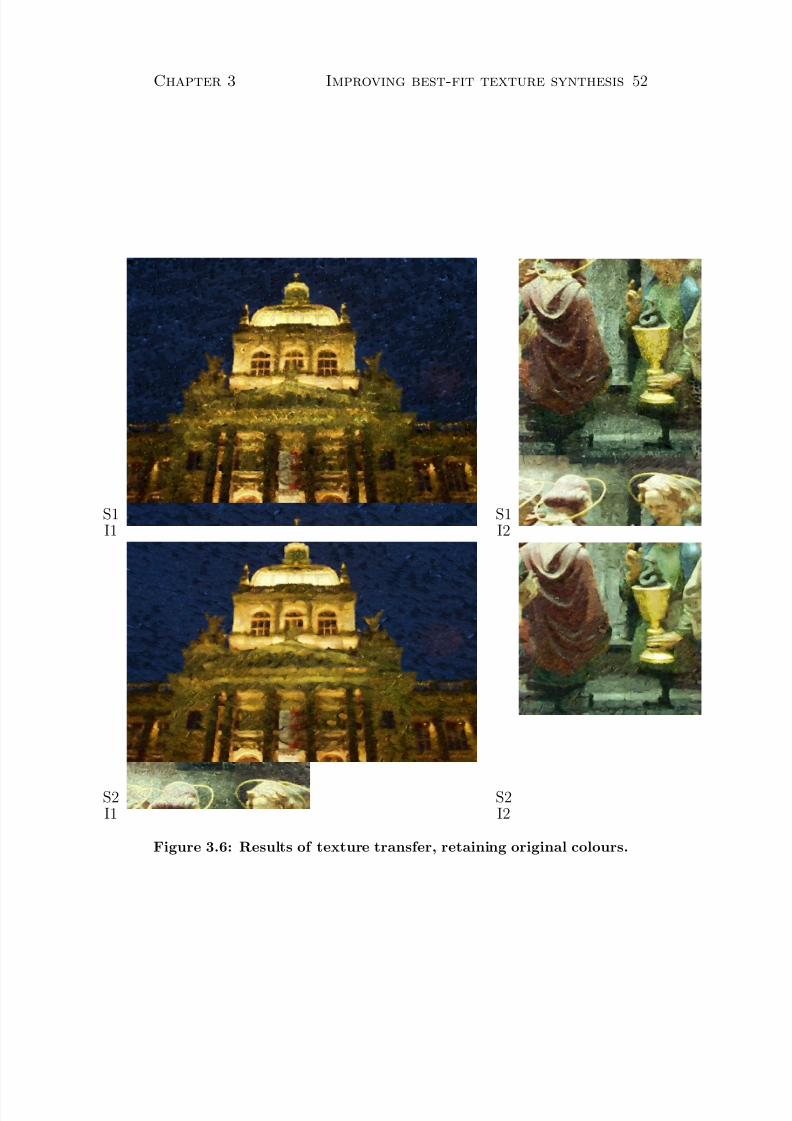
greater chance of finding correspondences. One simple way to do this is
to reduce the maps from colour to gray-scale, dividing the number of
dimensions by three. This was used to produce the results shown in
Figure 3.6. The input and output maps and the input texture were
reduced to gray-scale images. After synthesis, the colour from the
original output maps was copied to the synthesized images.
Using this process, the limited palette in the textures is not a problem.
The results are now quite faithful to the output map, however some
subtleties of colouration present in the textures have been lost.
8/20/2019 P. Harrison PhD Thesis
http://slidepdf.com/reader/full/p-harrison-phd-thesis 51/141
Chapter 3 Improving best-fit texture synthesis 51
S1I1
S1I2
S2I1
S2I2
Figure 3.5: Results of texture transfer.
8/20/2019 P. Harrison PhD Thesis
http://slidepdf.com/reader/full/p-harrison-phd-thesis 52/141
Chapter 3 Improving best-fit texture synthesis 52
S1I1
S1I2
S2I1
S2I2
Figure 3.6: Results of texture transfer, retaining original colours.

8/20/2019 P. Harrison PhD Thesis
http://slidepdf.com/reader/full/p-harrison-phd-thesis 53/141
Chapter 3 Improving best-fit texture synthesis 53
3.4 Plausible restoration
Texture synthesis has been previously applied to the removal of objects
on a homogeneous background by synthesizing a new section of that
background [Igehy and Pereira, 1997]. An example of this is shown in
Figure 3.7c. Texture transfer allows synthesis of a new background to
replace an object, even if the background is non-homogeneous.
Figure 3.7a shows a picture of a donkey standing in a field. In this
picture, the field is not homogeneous because of perspective distortion.
A feature map of the image (Figure 3.7b) was constructed manually,
with parts of the image equidistant from the camera having the same
value. The texture transfer variant just described was then used to
synthesize a new section of the background to replace the donkey, using
the rest of the background as input texture. The new section matches
with the existing background and follows the feature map. The result is
shown in Figure 3.7d.
3.5 Discussion
The algorithm described in this chapter used a variety of enhancements
to the original best-fit algorithm. Choosing pixel values in random order
eliminated the problem of skew. Garbage and repetition were also
reduced, but not eliminated entirely. Another way of looking at this is to
say that even with random ordering certain parts of a texture were
obsessively over-represented in the output. The import of this will be
explored further in Chapter 7.
The further change of using a robust Cauchy-based metric was required
to yield output that was a representative sample of the input. As this is
an unglamorous topic, and easily overlooked, it will be mentioned briefly

8/20/2019 P. Harrison PhD Thesis
http://slidepdf.com/reader/full/p-harrison-phd-thesis 54/141
Chapter 3 Improving best-fit texture synthesis 54
(a) (b)
(c) (d)
Figure 3.7: Example of object removal. (a) original image (fromIgehy and Pereira [1997]), (b) map, (c) object removed without usingmap, (d) object removed using map.
here that the use of the Cauchy distribution and other alpha-stabledistributions in places where the Gaussian distribution and its associated
least-squares criterion have formerly been used has yielded improvements
in robustness and performance to a wide range of signal processing tasks
[Nikias and Shao, 1995]. An ongoing shift away from use of the Gaussian
distribution may reasonably be expected in a variety of fields.
The next chapter describes software that allows the algorithm described
in this chapter to be used in everyday image manipulation tasks.

8/20/2019 P. Harrison PhD Thesis
http://slidepdf.com/reader/full/p-harrison-phd-thesis 55/141
Chapter 4
Adding best-fit texture
synthesis to the GIMP
In order to be useful, texture manipulation techniques need to integrate
with existing software. This chapter describes integration of the method
of the previous chapter into the GNU Image Manipulation Program
(GIMP, http://www.gimp.org/).
The GIMP was chosen because it is popular, and because it provides
facilities for extending its capabilities. The GIMP’s extensibility comes
in two forms, plug-ins and scripts. Plug-ins are written in C or C++,
and have low level access to image data structures. Scripts are written in
Scheme, Perl, or Python, and can be used to combine plug-ins and the
GIMP’s built-in tools to perform complex tasks.
The implementation of texture operations may be complex, but the
problems they solve are easy to understand. Thus their implementation
in software need not be hard to use. Care was taken to eliminate as many
parameters as possible. It is impolite to trouble people intent on their
task at hand with obscure mathematical details of the tools they use.
55

8/20/2019 P. Harrison PhD Thesis
http://slidepdf.com/reader/full/p-harrison-phd-thesis 56/141
Chapter 4Adding best-fit texture synthesis to the GIMP 56
Figure 4.1: The interface to the best-fit synthesis plug-in.
(a) (b)
Figure 4.2: Scripts using the best-fit plug-in, which also have simpleinterfaces: (a) enlarge an image, (b) remove a selection.
A 900 line GIMP plug-in (written in C++) was created to perform the
best-fit synthesis variant described in the previous chapter. This plug-in
can perform texture synthesis, texture transfer, and plausible restoration
of missing areas in an image. It can be obtained from
http://www.logarithmic.net/pfh/thesis (or the CD accompanying
this dissertation).
A screenshot of the plug-in’s user interface is shown in Figure 4.1. As
can be seen, the interface is straightforward, with a minimum of options.
By using the GIMP’s facility for selecting regions, the plug-in can be
used to synthesize texture over a specific area of an image. Plausible
restoration (as in Figure 3.7) is straightforward.

8/20/2019 P. Harrison PhD Thesis
http://slidepdf.com/reader/full/p-harrison-phd-thesis 57/141
Chapter 4Adding best-fit texture synthesis to the GIMP 57
The GIMP’s scripting facility can be used to automate use of the
plug-in. For example, a script was written to enlarge images while
retaining their texture and the sharpness of their edges (Figure 4.2a).
This script works by analogy: an enlarged version of the image is to the
image as the image is to a reduced version of the image. Texture transfer
is used, where the texture is the input image, the texture map is the
input image reduced in size and then restored to its original size (thus
losing high frequency components), and the output map is an enlarged
version of the input. The script uses a combination of the GIMP’s image
scaling function and the best-fit plug-in.
A second script was written to delete a selected region by synthesizing
surrounding texture on top of it (Figure 4.2b). The input texture is
simply a ring of specified thickness about the selection. Figure 4.3 shows
an example of this script in use.
4.1 Discussion
There is frequently a gap between the advanced algorithms published in
computer graphics journals and the less advanced tools available to
non-technical users. The availability of this best-fit implementation has
generated considerable interest and positive feedback from users of the
GIMP.
Ideally “advanced” tools such as this should disappear into the
background, doing their job without making a fuss about their
cleverness. The plug-in just described is an everyday tool for everyday
tasks.

8/20/2019 P. Harrison PhD Thesis
http://slidepdf.com/reader/full/p-harrison-phd-thesis 58/141
Chapter 4Adding best-fit texture synthesis to the GIMP 58
Figure 4.3: Remove-selection script in action.

8/20/2019 P. Harrison PhD Thesis
http://slidepdf.com/reader/full/p-harrison-phd-thesis 59/141
Chapter 5
Patchwork texture synthesis
Many texture synthesis techniques copy large sections of the sample
texture to the output. This can be seen, for example, in the results of
the best-fit method (including the variant described in Chapter 3). A
number of texture synthesis methods make the copying process explicit.
For example, in Efros and Freeman’s “Image Quilting” method [Efros
and Freeman, 2001, Liang et al., 2001] an overlapping grid of tiles is
produced. Each tile is simply copied from the sample texture. Tiles are
chosen so that their overlapping regions match as closely as possible.
The Chaos Mosaic method of Xu et al. [2000] takes the idea of copying
from the sample texture one step further, with tiles chosen at random
from the sample texture randomly pasted onto the output image. No
attempt is made to match tiles to each other. Feathering is used to try
to disguise tile borders. However, as shall be shown in this chapter,
feathering produces visible artifacts.
This chapter examines whether copying random sections of a sample
texture is all that is necessary for texture synthesis. A simple method of
texture synthesis is proposed, based on random copying. The texture
synthesis method is applied to images and to video. Its extension to
59
8/20/2019 P. Harrison PhD Thesis
http://slidepdf.com/reader/full/p-harrison-phd-thesis 60/141
Chapter 5 Patchwork texture synthesis 60
texture transfer is also described.
5.1 Method
The texture synthesis method presented in this chapter simply copies
random patches of the input to the output, so that the output is
completely covered. The edges of these patches are blended together so
as to be invisible.
The difficulty lies in making edges within the output invisible. Several
types of edges are illustrated in Figure 5.1. As can be seen, a sharp
transition (Figure 5.1a) is clearly visible, while a gradual transition
(Figure 5.1b) looks duller than the original texture. This kind of
transition, sometimes called feathering, was used by Xu et al. [Xu et al.,
2000] in their “Chaos Mosaic” texture synthesis method. This dullness
can be removed by controlling the standard deviation of pixels in the
transition (as described in the next section), producing an invisible join
(Figure 5.1c).
An irregular pattern of patches is used, as the human eye is skilled at
discerning regular patterns. A Voronoi diagram, based on a set of
randomly chosen points, produces a patchwork that is sufficiently
irregular.
5.2 Image texture synthesis
In this section, texture synthesis on images is considered. Symbols used
in this section are listed in Table 5.1.
First, define the Voronoi cells that are to be used as patches. Choose n

8/20/2019 P. Harrison PhD Thesis
http://slidepdf.com/reader/full/p-harrison-phd-thesis 61/141
Chapter 5 Patchwork texture synthesis 61
(a)
(b)
(c)
Figure 5.1: Joining one texture patch to another by (a) a sharp tran-sition, (b) a gradual transition and (c) a gradual transition controllingfor standard deviation.
O(x) Output imageI (x) Input image
pi A set of points in the output imageq i A set of points in the input imagef Parameter specifying patch border sharpness
d(a, b) Euclidean distance between points a and b
Table 5.1: List of symbols.

8/20/2019 P. Harrison PhD Thesis
http://slidepdf.com/reader/full/p-harrison-phd-thesis 62/141
Chapter 5 Patchwork texture synthesis 62
(a) (b) (c)
Figure 5.2: Example of patch shapes about the points pi for (a) f = 2,(b) f = 6 and (c) f = 20
points pi in the output image O(x). The points pi form the centers of
Voronoi cells, and should be chosen to cover the output evenly. One
simple way to achieve this is to choose jittered grid points. The size of
the grid determines the approximate size of each cell, as well as the
number of points required.
Also choose n points q i from the input image I (x) at random. These are
used to specify the part of the texture sample copied into each patch.
The points must be chosen such that for all points x in or near the
Voronoi cell of pi the point x − pi + q i lies within the input image. Thisis necessary to ensure that the portion of the texture sample copied to
each patch lies within the texture sample’s border.
Let d((x1, y1), (x2, y2)) be the Euclidean distance between two points.
Let a be the average colour of the input image. Let f be a parameter
defining the sharpness of the edges of the patches (the effect of this
parameter is illustrated in Figure 5.2). Assign each Voronoi cell a weight
wi(x) at each point x in the output image
wi(x) = d(x, pi)−f (5.1)
Then the value of each pixel in the output image is calculated using

8/20/2019 P. Harrison PhD Thesis
http://slidepdf.com/reader/full/p-harrison-phd-thesis 63/141
Chapter 5 Patchwork texture synthesis 63
O(x) =
ni=1(I (x − pi + q i) − a)wi(x)
ni=1 wi(x)2
+ a (5.2)
In this equation, the divisor rescales the result so that its standard
deviation is the same as that of the input image. Subtracting out and
then adding back the average a ensures that the output image has the
same average colour as the input. For efficiency, terms with small weight
may be omitted from the summations.
5.2.1 Results
The test suite of images (Figure A.1) was used to test the image
synthesis technique. The results of synthesis are shown in Figure 5.3.
Many of the synthesized textures (S1, S2, C1, E1, E2, E3) do not
contain any obvious artifacts and are not obviously synthetic. However,
there is a tendency for large scale structure in the input to be lost,
producing somewhat fragmentary or “busy” results. Best results were
obtained where the texture did not have large structures, such as objects
(C3), cracks (C2, C4), or tiling elements (T1, T2). Random choice of
patches is therefore not sufficient for synthesis of all textures, but is
practical for a subset of textures.

8/20/2019 P. Harrison PhD Thesis
http://slidepdf.com/reader/full/p-harrison-phd-thesis 64/141
Chapter 5 Patchwork texture synthesis 64
S1 S2 C1
C2 C3 C4
E1 E2 E3
T1 T2
N1 N2 N3
Figure 5.3: Results with f = 6, and a grid size of 64 pixels.
8/20/2019 P. Harrison PhD Thesis
http://slidepdf.com/reader/full/p-harrison-phd-thesis 65/141
Chapter 5 Patchwork texture synthesis 65
5.2.2 GIMP integration
The essential part of the method described in this chapter is the
disguising of edges by controlling the standard deviation of pixel values.
The GIMP, as with most image manipulation programs, uses alpha
blending. As discussed earlier, this produces a result with reduced
standard deviation. The effect can be removed by slightly altering one of
the layers based on the alpha values, as shall now be shown.
Let c1 and c2 be the upper and lower layers being blended respectively, α
the alpha value, and cavg the average colour of the upper layer. The
standard method of alpha blending is
cout = c1α + c2(1 − α) (5.3)
with cout having standard deviation
σout = σin
α2 + (1 − α)2 (5.4)
Thus σout will be less then σin for α values not equal to zero or one. c1
can be rescaled by a factor f to counteract this effect. It is required that
σout = σin, so
σin = σin
f 2α2 + (1 − α)2 (5.5)
producing a scaling factor of
f =
2
α − 1 (5.6)

8/20/2019 P. Harrison PhD Thesis
http://slidepdf.com/reader/full/p-harrison-phd-thesis 66/141
Chapter 5 Patchwork texture synthesis 66
Figure 5.4: Patchwork synthesis script.
The correction is therefore to change the value of c1 as follows:
c1 ← f (c1 − cavg) + cavg (5.7)
A 175 line C plug-in was written to provide this. It can be obtained
from http://www.logarithmic.net/pfh/thesis (or the CD
accompanying this dissertation). In combination with the GIMP’s built
in facility for alpha blending and copying and pasting feathered
selections, this provides a method for rearranging parts of an image
without modifying its texture.
One problem with this approach is that the colour can be rescaled below
zero or above the maximum allowed brightness, and thus need to be
clipped. Ideally, clipping would occur after alpha blending. This would
require a modification to the GIMP itself, rather than a plug-in.
A simple script was written to synthesize textures by randomly copying
and pasting feathered selections from a texture to a new image, making
use of the plug-in (Figure 5.4). The results are similar to those seen in
Figure 5.3.

8/20/2019 P. Harrison PhD Thesis
http://slidepdf.com/reader/full/p-harrison-phd-thesis 67/141
Chapter 5 Patchwork texture synthesis 67
patch-method-1.mpg patch-method-2.mpg(a) (b)
Figure 5.5: Video cubes illustrating the cell shapes of two differentvideo synthesis methods (the vertical axis is time). These videos maybe obtained from http://www.logarithmic.net/pfh/thesis (or the CDaccompanying this dissertation).
5.3 Video texture synthesis
In this section, the texture synthesis method is extended to video. The
obvious way to approach video texture synthesis is to treat the temporal
dimension as just another spatial dimension, producing a three
dimensional mosaic of patches. This is illustrated in Figure 5.5a. It has
the drawback that any static elements in the video will become transient
in the output. It is therefore proposed to treat the time dimension
separately. Patches are fixed between frames, and a separate
compositing step is performed in the time dimension, as illustrated in
Figure 5.5b. This will preserve any static elements in the texture.
The video texture synthesis method consists of two stages. In the first
stage, a set of video sequences are constructed from frames of the inputvideo. In these intermediate sequences, no re-arrangement within each
frame takes place, just a re-arrangement of the frames themselves. In the
second stage, each frame of the output sequence is constructed from the
corresponding frames of the intermediate sequences, using the image
synthesis method described earlier in this chapter.
To generate each intermediate sequence, n frames pi are first chosen in
the intermediate sequence, and n corresponding frames q i are chosen in

8/20/2019 P. Harrison PhD Thesis
http://slidepdf.com/reader/full/p-harrison-phd-thesis 68/141
Chapter 5 Patchwork texture synthesis 68
the input sequence. The intermediate sequence is generated as a series of
transitions between each frame pi and its successor pi+1.
First, define weights for a smooth transition between pi and pi+1
w1 = 1
2 +
1
2cos(πu) (5.8)
w2 = 1
2 − 1
2cos(πu) (5.9)
where u is the position within the interval [ pi, pi+1]
u = t − pi
pi+1 − pi
(5.10)
Also calculate the average value of each pixel in the input sequence over
time, forming an average image A(x). Then the intermediate sequence
N (x, t) may be synthesized from the input sequence I (x, t) within theinterval using
N (x, t) = w1I (x, t − pi + q i) + w2I (x, t − pi+1 + q i+1) − A(x)
w21 + w2
2
+ A(x)
(5.11)
In this equation, each pixel in each intermediate frame is produced by
combining pixels from two source sequences. The standard deviation of
each pixel is preserved in the result.
Piecing all the intervals together gives a full intermediate sequence.
The output sequence is generated from a set of intermediate sequences.
Each frame of the output is constructed by piecing together patches
sampled from the corresponding frames of the intermediate sequences as

8/20/2019 P. Harrison PhD Thesis
http://slidepdf.com/reader/full/p-harrison-phd-thesis 69/141
Chapter 5 Patchwork texture synthesis 69
leaves.mpg clouds.mpg fire.mpg
leaves-patched.mpg clouds-patched.mpg fire-patched.mpg
Figure 5.6: Input video cubes (top row) and corresponding syntheticvideo cubes (bottom row). These videos may be downloaded from
http://www.logarithmic.net/pfh/thesis (or the CD accompanyingthis dissertation).
in the image synthesis method. Each intermediate frame contributes one
patch to the output frame. Each frame in the output is synthesized
using the same arrangement of patches.
For efficiency the two stages of synthesis can be combined, so that the
pixel values in the intermediate sequences are only ever calculated as
needed.
5.3.1 Results
Results are shown in Figure 5.6. All results are tilable video loops. Thefirst video produced good results. That is, there are no obvious artifacts
and the video is not obviously synthetic. The second was less
satisfactory, the patches are clearly visible. This is because the
movement of the clouds reveals the pattern of patches. The third video
also produced reasonable results, although there are some artifacts where
bright flame occurred at the edge of a patch.

8/20/2019 P. Harrison PhD Thesis
http://slidepdf.com/reader/full/p-harrison-phd-thesis 70/141
Chapter 5 Patchwork texture synthesis 70
5.4 Texture transfer
In this section, the texture synthesis method described in the previous
sections will be extended to texture transfer. This will first be described
in the domain of images, then generalized to video.
To perform texture transfer, two images are required. As before, a
texture image is required (I (x)). Additionally a pattern image is
necessary (P (x)). The pattern image defines the pattern of texture
desired in the output. For example, by using a painting as the image
texture and a photograph as the pattern image a synthetic painting of
the photograph could be created.
Patches are again defined in terms of a Voronoi diagram. However, the
points q i in the input texture are no longer chosen randomly. Instead,
each is chosen to minimize the sum of squared differences between the
patch of the pattern image around pi and the patch of input texture
around q i.
Finding the exact best match to each patch often means that a
particular area of the texture sample is repeated many times in the
output. A solution to this problem is to consider only a random subset
of points in the image as possibilities for each point q i. This also yields a
substantial speed increase.
The output to be synthesized is no longer homogeneous. The average
pixel value varies from place to place. During synthesis this means that
rather than using an overall average, a localized average must be used.
One way to do this is to calculate an average ai of each patch. The
output can then be calculated from
O(x) =n
i=1(I (x
− pi + q i)
−ai)wi(x) n
i=1 wi(x)2 +n
i=1 aiwi(x)ni=1 wi(x) (5.12)

8/20/2019 P. Harrison PhD Thesis
http://slidepdf.com/reader/full/p-harrison-phd-thesis 71/141
Chapter 5 Patchwork texture synthesis 71
This is very similar to Equation 5.2, the only difference being the
calculation of the average.
This transfer technique may also be applied to video. For example, to
produce an image with animated texture, the pattern image P (x) might
be matched against the average frame A(x). The video texture synthesis
method described in section 5.3 can then be applied.
5.4.1 Results
Results are shown in Figure 5.7, based on the texture transfer test-suite
(Figure A.2). As a pre-processing step, the pattern images were rescaled
so that they had the same average colour and colour range as the texture
images. These images took longer to produce than the texture synthesis
images, as selecting each patch required searching the texture image.
As with the best-fit method, reducing the dimensionality of the search
space can be used to improve results (see Section 3.3.1). The texture
and pattern used for texture transfer were reduced to gray-scale images
before texture transfer, and the original colour from the pattern image
reapplied to the output. This produced the results in Figure 5.8.
An example of video texture transfer is shown in Figure 5.9. The texture
used was the video of leaves in Figure 5.6.

8/20/2019 P. Harrison PhD Thesis
http://slidepdf.com/reader/full/p-harrison-phd-thesis 72/141
Chapter 5 Patchwork texture synthesis 72
S1I1
S1I2
S2I1
S2I2
Figure 5.7: Texture transfer with f = 2, and a grid size of 16 pixels.

8/20/2019 P. Harrison PhD Thesis
http://slidepdf.com/reader/full/p-harrison-phd-thesis 73/141
Chapter 5 Patchwork texture synthesis 73
S1I1
S1I2
S2I1
S2I2
Figure 5.8: Texture transfer with colour copied directly from pat-tern.
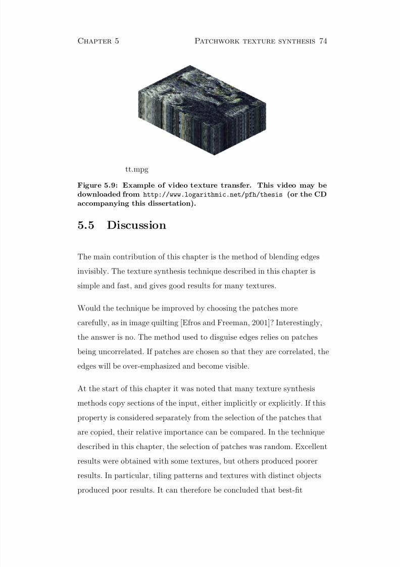
8/20/2019 P. Harrison PhD Thesis
http://slidepdf.com/reader/full/p-harrison-phd-thesis 74/141
Chapter 5 Patchwork texture synthesis 74
tt.mpg
Figure 5.9: Example of video texture transfer. This video may bedownloaded from http://www.logarithmic.net/pfh/thesis (or the CDaccompanying this dissertation).
5.5 Discussion
The main contribution of this chapter is the method of blending edges
invisibly. The texture synthesis technique described in this chapter is
simple and fast, and gives good results for many textures.
Would the technique be improved by choosing the patches more
carefully, as in image quilting [Efros and Freeman, 2001]? Interestingly,
the answer is no. The method used to disguise edges relies on patches
being uncorrelated. If patches are chosen so that they are correlated, the
edges will be over-emphasized and become visible.
At the start of this chapter it was noted that many texture synthesis
methods copy sections of the input, either implicitly or explicitly. If this
property is considered separately from the selection of the patches that
are copied, their relative importance can be compared. In the technique
described in this chapter, the selection of patches was random. Excellent
results were obtained with some textures, but others produced poorer
results. In particular, tiling patterns and textures with distinct objects
produced poor results. It can therefore be concluded that best-fit

8/20/2019 P. Harrison PhD Thesis
http://slidepdf.com/reader/full/p-harrison-phd-thesis 75/141
Chapter 5 Patchwork texture synthesis 75
selection of patches can only improve textures such as these.
This chapter and the preceding ones have described methods of creating
new images with a given texture. The next chapter looks at the
restoration of the texture of existing images where that texture has been
degraded by noise.

8/20/2019 P. Harrison PhD Thesis
http://slidepdf.com/reader/full/p-harrison-phd-thesis 76/141
Chapter 6
Plausible restoration of noisy
images
The values of pixels in an image may, for various reasons, be known only
imprecisely. If so, the texture of that image may be used to help
estimate the true pixel values. In a textured image the value of one pixel
may give clues as to the values of other pixels. This chapter describes
how a texture model may be used to find the most likely pixel values of
an image, where only upper and lower bounds on these values are
known. A variant that can remove Gaussian noise is also described.
Imprecise knowledge of an image usually takes the form of an image with
additive noise. This noise might be generated as a result of storing an
image in a lossy format such as JPEG or GIF, introduced while
converting it from analogue to digital form, or produced by an analogue
device. The amount of noise may depend on the position in the image,
or even the content of the image. Restoration of images stored in lossy
formats is of particular interest, given the large number of these images
that now exist (for example, on the World-Wide Web).
The novel feature introduced in this chapter, as compared to other
76

8/20/2019 P. Harrison PhD Thesis
http://slidepdf.com/reader/full/p-harrison-phd-thesis 77/141
Chapter 6 Plausible restoration of noisy images 77
methods of noise removal, is the use of complex texture models tailored
to each individual image. The kind of textural details seen in an
un-degraded part of an image may reasonably be expected to occur in
degraded parts. Texture that occurs in the form of large variations may
also occur in small details occluded by noise. These ideas can be
expressed in terms of texture modelling, allowing more accurate
restoration of images.
To attempt removal of additive noise from an image, two things must
first be stated:
1. The set of possible values for each pixel, and how likely each of
these values is (in other words, the amount and nature of noise).
2. The ways in which pixels may be related to one another (in other
words, what kinds of texture the image may have).
Given these two statements, the most likely image and image texture
may be found.1 The way the two statements are made is crucial. They
must be precise enough that the result is useful, but must also be stated
in a way that affords computation of the result in reasonable time. The
difficulty lies in finding a useful trade-off between these two constraints.
As was noted in Section 2.3.2 of the literature review, most methods of
noise removal dull the image. The method described here (as with thatof Meyer and Tischer [1998]) will not always dull images. While it uses a
texture model, it does not require this model to be specified a priori.
The method is simple in form, and is applicable to the general problem
of additive noise removal.
The method of this chapter uses the following choice of statements:
1
Most existing noise removal techniques (see Section 2.3.2) can be defined by twostatements of this form, though this is often not done explicitly.
8/20/2019 P. Harrison PhD Thesis
http://slidepdf.com/reader/full/p-harrison-phd-thesis 78/141
Chapter 6 Plausible restoration of noisy images 78
1. Each pixel value lies within a specific range, but is equally likely to
take any value within that range.
2. The image has texture that may be described in terms of causalprediction.
The next two sections detail and justify this choice.
6.1 Pixel values
Each pixel value is taken to lie within a specific range, but to be equally
likely to take any value within that range. This choice does not compete
with the texture model to explain small variations, where noise will
mean that almost nothing is known anyway. However it totally rules out
consideration of large changes to pixel values, so the texture model need
not model large changes, such as edges, with total accuracy.
The pixel ranges may be unbounded on one or both sides. For example,
a photograph may have been over-exposed when it was taken (the
amount of light incident on some areas of the film exceeding the film’s
range of measurement). Within regions of over-exposure it is known only
that the true pixel values exceed a certain amount. There may also be
artifacts such as spots obscuring parts of the image. A pixel within this
kind of area may be considered to be equally likely to take any value.
(This is similar to the technique for erasing objects from images
described in Chapter 3. Unlike the technique of Chapter 3 the result
may exceed the dynamic range of the input texture sample.)
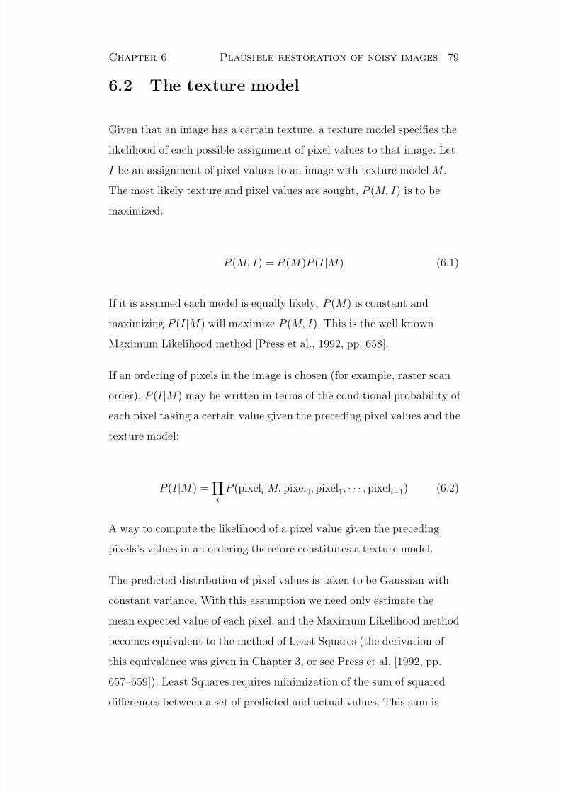
8/20/2019 P. Harrison PhD Thesis
http://slidepdf.com/reader/full/p-harrison-phd-thesis 79/141
Chapter 6 Plausible restoration of noisy images 79
6.2 The texture model
Given that an image has a certain texture, a texture model specifies the
likelihood of each possible assignment of pixel values to that image. Let
I be an assignment of pixel values to an image with texture model M .
The most likely texture and pixel values are sought, P (M, I ) is to be
maximized:
P (M, I ) = P (M )P (I |M ) (6.1)
If it is assumed each model is equally likely, P (M ) is constant and
maximizing P (I |M ) will maximize P (M, I ). This is the well known
Maximum Likelihood method [Press et al., 1992, pp. 658].
If an ordering of pixels in the image is chosen (for example, raster scan
order), P (I |M ) may be written in terms of the conditional probability of
each pixel taking a certain value given the preceding pixel values and thetexture model:
P (I |M ) =i
P (pixeli|M, pixel0, pixel1, · · · , pixeli−1) (6.2)
A way to compute the likelihood of a pixel value given the preceding
pixels’s values in an ordering therefore constitutes a texture model.
The predicted distribution of pixel values is taken to be Gaussian with
constant variance. With this assumption we need only estimate the
mean expected value of each pixel, and the Maximum Likelihood method
becomes equivalent to the method of Least Squares (the derivation of
this equivalence was given in Chapter 3, or see Press et al. [1992, pp.
657–659]). Least Squares requires minimization of the sum of squared
differences between a set of predicted and actual values. This sum is

8/20/2019 P. Harrison PhD Thesis
http://slidepdf.com/reader/full/p-harrison-phd-thesis 80/141
Chapter 6 Plausible restoration of noisy images 80
called a “merit function”.
The specific predictor used in this chapter is a weighted sum of a set of
values computed from neighbours of the pixel that are in its “past”, with
the pixels being ordered in a raster scan. The values might simply be the
values of the pixel’s past neighbours (producing a linear predictor).
Other values might result from multiplying several values together, or
applying some non-linear function to a value, or combining values in
some other way. With sufficient values, any function of the anti-causal
neighbours may be approximated to arbitrary accuracy with a weighted
sum such as this.
Let V 1(s) . . . V n(s) be the set of values used for prediction of the pixel
I (s), and w1 . . . wn be the corresponding weights. The predictor is:
p(s) = w1V 1(s) + w2V 2(s) · · · + wnV n(s) (6.3)
When calculating the values V n at the edges of the image, the well
known reflection technique may be used. If the image is tilable, tiling
may be used instead.
The merit function is:
s∈ΩI
(I (s)−
p(s))2 (6.4)
The weights of the model wi and the pixel values I (s) (within the
specified bounds) are chosen so as to minimize this merit function.
8/20/2019 P. Harrison PhD Thesis
http://slidepdf.com/reader/full/p-harrison-phd-thesis 81/141
Chapter 6 Plausible restoration of noisy images 81
6.3 Minimization algorithm
The merit function may be minimized numerically. An arbitrary initial
image is chosen (within the specified bounds on each pixel), then a two
step process is followed: first an optimum model is found given the
current image, then an improved image is found given that model. This
process is iterated until it converges.
In the first step, the optimum model for the current image may be found
precisely. When minimized, the merit function will have zero partial
derivative with respect to each model weight. Each partial derivative is a
linear function of the model weights. Equating each derivative to zero
gives a set of linear equations. These may be solved to find the optimum
model.
In the second step the optimum image is approximated numerically, as
finding the optimum analytically is difficult. A multigrid method is used,
as described in Press et al. [1992, pp. 871–887 ]. First a scaled downimage of the input is optimized, then successively larger versions. At
each scale the optimization is performed via gradient descent.
The multigrid method is necessary so that large features can be
optimized within a reasonable time. For example, gradients that have
been converted to a series of steps by palettization (as in Figure 6.3)
would take a long time to optimize at maximum scale.
Three images undergo scaling: an image of the minimum possible values,
an image of the maximum possible values, and the current best estimate
of the optimum image. The best-estimate image is scaled up by means of
bi-linear interpolation, and scaled down by its adjoint operator, as in
Press et al. [1992, pp. 875–876]. The minimum and maximum images
only ever need to be scaled down, as they are never modified. When
scaling down the minimum image, each pixel in the scaled down image

8/20/2019 P. Harrison PhD Thesis
http://slidepdf.com/reader/full/p-harrison-phd-thesis 82/141
Chapter 6 Plausible restoration of noisy images 82
Figure 6.1: Grid positions when scaling an image. A pixel in thecoarser grid has been highlighted in dark gray, and the pixels itoverlaps in the finer grid highlighted in light gray.
takes the maximum of the nine pixels it overlaps in the original image
(as illustrated in Figure 6.1). Similarly each pixel in the scaled down
maximum image takes the minimum of the nine pixels it overlaps in the
original. Where the value of a scaled down minimum pixel exceeds the
value of its corresponding scaled down maximum, both are replaced by
the value of the corresponding scaled down best-estimate pixel.
This method of scaling ensures that pixels in the best-estimate image
almost never scale up to a value outside of the bounds posed by the
minimum and maximum images. While this method is ad-hoc it should
not affect the outcome, as the final step is to optimize the image at its
original scale.
6.4 Results
The standard “Lena” image [Sjooblom, 1972] was used to test the
method. Four different versions of Lena were used:
A. Lena encoded with a palette of only 16 gray levels. The levels were
evenly spaced and the image was not dithered.
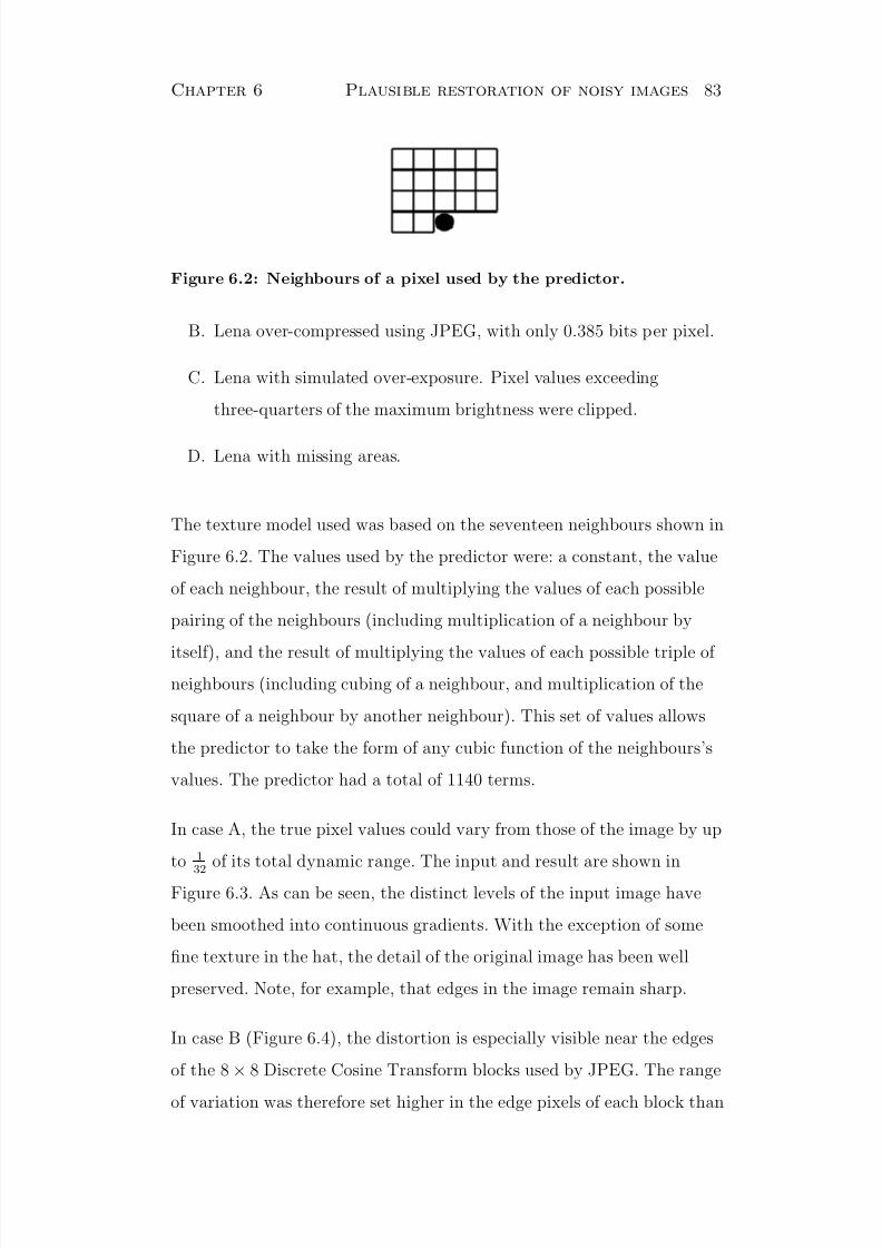
8/20/2019 P. Harrison PhD Thesis
http://slidepdf.com/reader/full/p-harrison-phd-thesis 83/141
Chapter 6 Plausible restoration of noisy images 83
Figure 6.2: Neighbours of a pixel used by the predictor.
B. Lena over-compressed using JPEG, with only 0.385 bits per pixel.
C. Lena with simulated over-exposure. Pixel values exceeding
three-quarters of the maximum brightness were clipped.
D. Lena with missing areas.
The texture model used was based on the seventeen neighbours shown in
Figure 6.2. The values used by the predictor were: a constant, the value
of each neighbour, the result of multiplying the values of each possible
pairing of the neighbours (including multiplication of a neighbour by
itself), and the result of multiplying the values of each possible triple of neighbours (including cubing of a neighbour, and multiplication of the
square of a neighbour by another neighbour). This set of values allows
the predictor to take the form of any cubic function of the neighbours’s
values. The predictor had a total of 1140 terms.
In case A, the true pixel values could vary from those of the image by up
to 1
32 of its total dynamic range. The input and result are shown in
Figure 6.3. As can be seen, the distinct levels of the input image have
been smoothed into continuous gradients. With the exception of some
fine texture in the hat, the detail of the original image has been well
preserved. Note, for example, that edges in the image remain sharp.
In case B (Figure 6.4), the distortion is especially visible near the edges
of the 8 × 8 Discrete Cosine Transform blocks used by JPEG. The range
of variation was therefore set higher in the edge pixels of each block than

8/20/2019 P. Harrison PhD Thesis
http://slidepdf.com/reader/full/p-harrison-phd-thesis 84/141
Chapter 6 Plausible restoration of noisy images 84
Input image Result
A 34.29 34.92
B 33.73 33.15
C 34.41 37.39D 29.01
Table 6.1: PSNR in decibels, as compared to the original Lena im-age.
the other pixels, and higher still in the corner pixels. Pixels in the
corners were allowed to vary by up to 12% of the image’s total dynamic
range, pixels on the edges were allowed to vary by 8%, and the
remaining pixels 4%. In the result, the “blockiness” of the input has
been largely removed. Better results could undoubtedly be obtained by
more accurately modelling JPEG quantization.
In case C (Figure 6.5), the uncertainty lies in the value of pixels in the
over-exposed regions. In these regions the pixels could originally have
had any value brighter than their current value. The reconstruction is
not perfect, but is a definite improvement on the clipped image. The
reconstruction of a fine light edge about the bottom and rear of the hat
is a notable success (see the detail image), as is the reconstruction of
Lena’s left eye.
In case D (Figure 6.6), pixel values in the missing regions may have any
value. The overall structure of restored areas is reasonably plausible, but
they are implausibly smooth and therefore stand out. It has also failedto extend sharp edges into the restored areas. Also shown in the figure is
the result of using the best-fit synthesis technique described in
Chapter 3. This highlights the difference between the most likely
restoration and a randomly sampled “plausible” restoration. The best-fit
method has invented details that are plausible in textural terms, and is
also appropriately rough.

8/20/2019 P. Harrison PhD Thesis
http://slidepdf.com/reader/full/p-harrison-phd-thesis 85/141
Chapter 6 Plausible restoration of noisy images 85
Input Result
detail: detail:
Figure 6.3: Input and result for test case A.
The Peak-Signal to Noise Ratio2 for each case is listed in Table 6.1.
Though only an approximation of the perceived image degradation
[Bhaskaran and Konstantinides, 1995, pp. 9], the PSNR is a simple and
objective measure. The PSNR improved slightly for image A, and
substantially for image C. The PSNR of Image B was slightly reduced.
A better model of the JPEG quantization algorithm may produce better
results.
2For 8-bit per pixel images having a noise of standard deviation σ, the PSNR indecibels is 20 log10
255
σ .
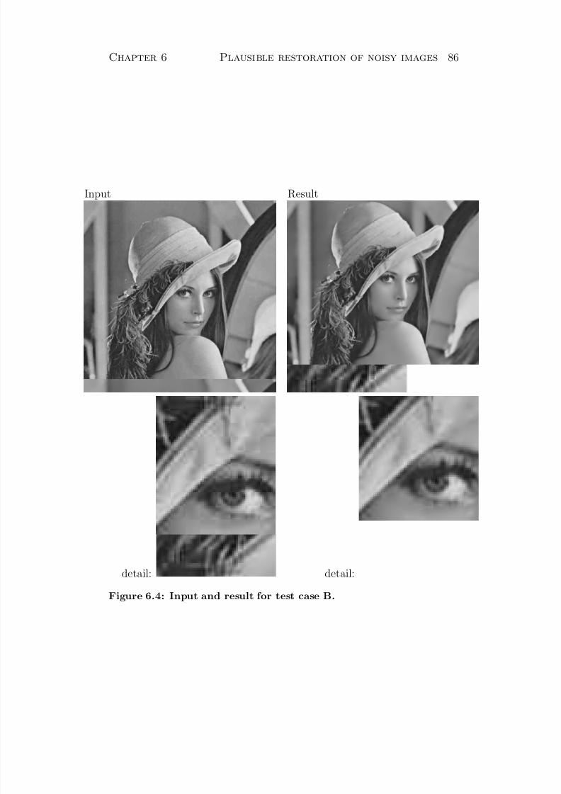
8/20/2019 P. Harrison PhD Thesis
http://slidepdf.com/reader/full/p-harrison-phd-thesis 86/141
Chapter 6 Plausible restoration of noisy images 86
Input Result
detail: detail:
Figure 6.4: Input and result for test case B.

8/20/2019 P. Harrison PhD Thesis
http://slidepdf.com/reader/full/p-harrison-phd-thesis 87/141
Chapter 6 Plausible restoration of noisy images 87
Input Result
detail: detail:
Figure 6.5: Input and result for test case C.

8/20/2019 P. Harrison PhD Thesis
http://slidepdf.com/reader/full/p-harrison-phd-thesis 88/141
Chapter 6 Plausible restoration of noisy images 88
Input Result
Best-fit synthesis result
Figure 6.6: Input and result for test case D, and for comparison theresult of applying the best-fit technique of Chapter 3.
8/20/2019 P. Harrison PhD Thesis
http://slidepdf.com/reader/full/p-harrison-phd-thesis 89/141
Chapter 6 Plausible restoration of noisy images 89
6.5 A variant for the removal of Gaussian
noise
Suppose we have an image with noise added from a uniform Gaussian
noise source of known variance.3 When finding the most likely true
image, the variance of the noise at each pixel must be constrained to not
exceed the variance of the noise source (the noise in the image is the
difference between the true image and the noisy input image).
We can not calculate the variance of noise at a pixel in the imageexactly, but we may estimate it from the values of surrounding pixels.
To produce this estimate, a convolution of the squared noise image by a
Gaussian kernel is performed. This convolved image is then constrained
to at no point exceed the variance of the noise source.4 A kernel of size
σ = 8 was found to give good results.
As in the previous section, gradient descent was used to find the most
likely image. The noise within each pixel being independent of
surrounding pixels, a multi-scalar method need not be used. After each
step of the descent, where the estimated variance of a pixel exceeds the
variance of the noise source the pixel value is scaled such that its
variance equals that of the noise source.
3This is a well studied problem in the field of Image Processing, and applying thealgorithm of this chapter to it allows comparison with other noise removal algorithms.
However the main intent of this chapter is the framing of a qualitatively differentproblem, “plausible restoration”, rather than further investigation of well studied noiseremoval problems.
4This assertion that the noise is uniform is necessary because the texture model doesnot take into account that some areas of the image may be more variable than others.A better solution would be to simply constrain the overall variance of the noise, whileextending the texture model to include variations in the amount of variation. However,it is not clear how to pose such a texture model in a form that may be optimized withina reasonable time.

8/20/2019 P. Harrison PhD Thesis
http://slidepdf.com/reader/full/p-harrison-phd-thesis 90/141
Chapter 6 Plausible restoration of noisy images 90
6.5.1 Results
The same neighbourhood and predictor terms were used as before. The
version of Lena used was the same as that in Portilla et al. [2003]
(available from http://decsai.ugr.es/~javier/denoise). Portilla
et al. [2003] have confirmed that this version is the same as that used in
a number of other recent papers. The image is 8-bit per pixel, with 256
possible gray levels.
Results are shown in Figures 6.7 and 6.8. It can be seen that the method
has preserved sharp edges well, and has not introduced artifacts into the
image, although in Figure 6.8 there are some patches where noise has
not been sufficiently removed, giving a blotchy appearance.
The resulting PSNR for various levels of noise is listed in Table 6.2.
Results obtained by Portilla et al. [2003]’s steerable pyramid based noise
removal algorithm are listed for comparison (this is the best existing
Gaussian noise removal algorithm, by this metric, to the author’sknowledge). The method described here is not as good as Portilla et al.’s
in terms of PSNR. Note however that Portilla et al.’s method introduces
some slight ringing-type artifacts5, whereas the one described here does
not. In general, steerable pyramid methods are biassed towards
interpreting variations in an image as features from the pyramid, and
tend to sometimes infer these features where they are not present.
5See http://decsai.ugr.es/~javier/denoise/examples/simulated_noisy.
htm.

8/20/2019 P. Harrison PhD Thesis
http://slidepdf.com/reader/full/p-harrison-phd-thesis 91/141
Chapter 6 Plausible restoration of noisy images 91
σ Input image Result Portilla et al.
10 28.12 34.75
35.6115 24.61 32.82 33.9020 22.12 31.31 32.6625 20.22 30.09 31.69
Table 6.2: PSNR in decibels for the removal of various levels of Gaussian noise. Results obtained by Portilla et al. [2003] are listedfor comparison.
Input Result
detail: detail:
Figure 6.7: Input and result for Gaussian noise, σ = 10.

8/20/2019 P. Harrison PhD Thesis
http://slidepdf.com/reader/full/p-harrison-phd-thesis 92/141
Chapter 6 Plausible restoration of noisy images 92
Input Result
detail: detail:
Figure 6.8: Input and result for Gaussian noise, σ = 25.

8/20/2019 P. Harrison PhD Thesis
http://slidepdf.com/reader/full/p-harrison-phd-thesis 93/141
Chapter 6 Plausible restoration of noisy images 93
6.6 Discussion
The main limitation on the complexity of model used in this chapter was
the available computing power. Were unlimited computing power
available, a larger neighbourhood and higher-order terms would almost
certainly yield further improvement. Every pixel and its causal
neighbourhood in an image represents an observation of the image’s
texture, and an image of (say) 512 × 512 pixels contains a great many
such observations, so a texture model with a great many terms can be
supported without danger of over-fitting.
Previous methods of noise removal have adapted their model of texture
to images in simple ways, limiting their ability to restore features that
are unique to a particular image. The method given here does not have
this limitation. Increasing the order of the texture model should allow
further improvements.
While it has many more terms than previous models used for additivenoise removal, the texture model used here is not fully general. For full
generality, the texture model would need to be able to predict arbitrary
probability distributions. Specification and optimization of a model this
general is difficult. Lesser generalizations are possible, such as prediction
of the standard deviation of each pixel in addition to the expected value,
or use of robust merit functions based on L1, Huber functions (as in
Rudin et al. [1992] and Llados-Bernaus et al. [1998]), or the Cauchy
based metric derived in Chapter 3.
An image restoration technique that can invent details is slightly
dangerous. In places where restoration must be reliable, such as
medicine or the military, such a method should only be used with care.
However, a technique that tailors itself to an image to better restore its
specifics may provide enhancements otherwise impossible, which could

8/20/2019 P. Harrison PhD Thesis
http://slidepdf.com/reader/full/p-harrison-phd-thesis 94/141
Chapter 6 Plausible restoration of noisy images 94
be crucial in these places.
If compression artifacts can be removed as they were in this chapter, is
lossy compression easy? The standard assumption has been that lossy
compression requires a detailed model of human perception, taking into
account phenomena such as masking. What if compression artifacts arise
simply because the decoder produces images that lack textural
self-consistency, and that human perception is sensitive to this? Were
decoders to produce more plausible images given limited information,
detailed modelling of perception might become unimportant. The lossy
aspect of lossy compression might reduce to a simple form of
quantization, and the well-studied techniques of lossless compression
could be applied. This is, of course, highly speculative.
The method described in this chapter represents a generic method for
filling in gaps where a set of data has missing elements or is only known
imprecisely. It might, for example, be transferred to the audio domain to
reconstruct noisy or clipped recordings, or be applied to other time seriesdata.
8/20/2019 P. Harrison PhD Thesis
http://slidepdf.com/reader/full/p-harrison-phd-thesis 95/141
Chapter 7
Declarative texture synthesis
Previous chapters have examined texture operations based on
synthesizing texture given a sample . This chapter looks at how an
interesting class of textures may be designed using rules specifying which
elements in a pattern may be adjacent to one another. This is a slight
detour from the main thrust of this dissertation, which is concerned with
texture operations that model texture based on a sample of that texture,
but serves to place certain curious features of the best-fit synthesis
method in a wider context.
The approach of this chapter is to procedural texture synthesis as
declarative programming languages are to procedural programming
languages, and might therefore be called “declarative texture synthesis”.
In a procedural language, one specifies a step-by-step procedure by
which some output may be produced. In a declarative language, one
specifies a set of rules which constrain the output, and it is possible for
there to be multiple outputs. Similarly procedural texture synthesis
requires a step-by-step procedure for producing the texture to be
specified, whereas “declarative” texture synthesis requires a set of rules
that constrain the texture that may be produced.
95

8/20/2019 P. Harrison PhD Thesis
http://slidepdf.com/reader/full/p-harrison-phd-thesis 96/141
Chapter 7 Declarative texture synthesis 96
The specific type of rules considered here are specifications of a set of
tiles which are to be assembled into a pattern. Some rules will lead to
many possible results, some to just one possible result, and some to none
at all. If there are many possible results, one is chosen at random.
How simple can local rules of interactions be made, while still producing
interesting large-scale structure? The best-fit synthesis method bears
some resemblance to the assembling of a jigsaw puzzle, in that it involves
the fitting together of many small patches of pixels. If best-fit synthesis
is like a jigsaw puzzle, it is one with many different pieces, and it is not
therefore surprising that the results also can be complex. However, it is
shown in this chapter that even simple jigsaw pieces can result in
surprisingly complex forms.
7.1 Specification of the problem domain
The objective is to find a connected structure composed only of pieces
from a specified set. Pieces are based on squares or hexagons with edges
of various types. An edge of a certain type may only abut edges of some
other certain type. Some edges of a piece may be “empty”, and these
edges do not need to abut another piece. All other edges must abut an
appropriate opposite edge. Pieces may be rotated, but not flipped.
There are two possible types of edge:
• Like-compatible edges. These edges must abut another edge of the
same type, and will be denoted by numbers (1, 2, 3, . . . ) . “-” shall
denote an empty edge, which can also be seen as “like compatible”.
• Opposite-compatible edges. These edges must abut some different
type of edge, and will be denoted by letters, with each lower case

8/20/2019 P. Harrison PhD Thesis
http://slidepdf.com/reader/full/p-harrison-phd-thesis 97/141
Chapter 7 Declarative texture synthesis 97
letter compatible only with its corresponding upper-case (a, A, b,
B, c, C, . . . ).
A piece may be fully specified by a string listing its edges in clockwise
order. For example, --AaAa.
Were pieces of this type to be used in a physical jigsaw-like puzzle, edges
might be shaped as in Figure 7.1. Alternatively, an appropriate
arrangement of magnetic or electrical charges on each edge could be used
to ensure each edge type connects only to its intended other. If
subjected to random impulses of an appropriate magnitude such pieces
would, eventually, self-assemble. This would be interesting to attempt at
a molecular scale (see also Wolfram [2002, pp. 1193]).
Figure 7.1: The two types of edge, as jigsaw-puzzle type joins.
7.1.1 Relation to Markov Random Fields
Arrangement of tiles depends only on local interactions (the edges of tiles
must match), and may be used to define a Markov Random Field. The
likelihood of a particular tile being placed at a particular location could
be set to either zero, if the tile does not match surrounding edges, or one
divided by the number of tiles that could potentially be placed at that
location. Similarly the likelihood of an assemblage (of some given size)

8/20/2019 P. Harrison PhD Thesis
http://slidepdf.com/reader/full/p-harrison-phd-thesis 98/141
Chapter 7 Declarative texture synthesis 98
will be zero if there are edges that do not match, and non-zero otherwise.
7.2 Literature review
This chapter has one foot in the theoretical topic of tiling patterns, and
the other in the practical field of procedural texture synthesis. Some
surprising results from the field of tiling patterns will first be reviewed.
A brief overview of procedural texture synthesis will then be given.
7.2.1 Tiling patterns
Before the invention of the modern techniques of procedural texture
synthesis and tiling of images, one of the most common forms of
texturing was tiling patterns produced from small sets of tiles. Such
patterns were almost universally repeating patterns, though sometimes
of great intricacy.
It is now known that there exist tile sets that may be used to cover the
plane, but for which there are no arrangements of tiles that form a
repeating pattern. This has particularly been studied in the context of
“Wang tiles”. Wang tiles are much like the tile sets considered in this
chapter, but with the additional restrictions that the tiles are square,
and may not be rotated.1
The smallest known set of Wang tiles thatforce non-repetition was found by Culik [1996], and contains 13 tiles.2
1Careful choice of edge types allows one to force all tiles to follow a consistentorientation, so this is really a sub-set of the tile sets considered here.
2A somewhat pointless application of Wang tiles to texture synthesis was describedby Cohen et al. [2003], in which each tile is decorated with an image who’s bordersmatch those of the tiles that may abut it. This can be used to generate infinite, non-repeating texture. But so can a smaller set of tiles, so long as the edge constraints allowsome randomness in the choice of tiles. It is easy for a tile set to allow non-repeatingpatterns, the difficulty lies only in forcing non-repetition.

8/20/2019 P. Harrison PhD Thesis
http://slidepdf.com/reader/full/p-harrison-phd-thesis 99/141
Chapter 7 Declarative texture synthesis 99
If rotation and arbitrarily shaped tiles are allowed, tile sets that force
non-repetition containing as few as two tiles are known. Penrose’s “kites
and darts” are a well known example of this [Grunbaum and Shephard,
1987, pp.531]. It may be possible for a single tile to force non-repetitive
tiling, but no tile is currently known that has this property.
Once one realizes that non-repetitive tile sets are possible, one quickly
also realizes that there are tile set analogues for all kinds of systems.
Wang tile sets have been described that find prime numbers, enumerate
the Fibonacci sequence, and simulate Turing machines and cellular
automata [Grunbaum and Shephard, 1987, pp.604–606]. The ability of
Wang tiles to simulate Turing machines shows that assembly of tile sets
is a form of universal computation.
We may then ask whether randomly chosen tile sets commonly lead to
complex computations, or whether this is simply a pathological case.
This is a question not of existence but of likelihood, and requires
computational experiments rather than mathematical deduction, a formof investigation championed by Stephen Wolfram [2002]. Much of what
Wolfram has to say is relevant to this chapter, so his theories will now be
described in some detail.
Wolfram examined the general behavior of many discrete systems using
computational experiments, though with a particular focus on “cellular
automata”, a form of causal Markov Random Field. The sheer breadth
of Wolfram’s investigations show that his observations have some
generality, and we may reasonably expect them to apply to tiling
patterns.
Wolfram found that an enumeration of the simplest possible rules for a
given class of system will commonly contain systems having surprisingly
diverse behaviors. He identifies four basic classes of behavior:
8/20/2019 P. Harrison PhD Thesis
http://slidepdf.com/reader/full/p-harrison-phd-thesis 100/141
Chapter 7 Declarative texture synthesis 100
1. Repetitive: The system repeats within a finite time.
2. Nested: The system produces a self-similar fractal pattern.
3. Autoplectic: The system produces pseudo-random output.
4. Complex: The system produces a diversity of behaviors.
Particle-like entities called “gliders”, with complex interaction
rules, often occur in such systems.3
Systems with more complex rules chosen at random were also found to
display these same classes of behavior. The complexity of the rules of a
system appeared to have little effect on the complexity of their behavior.
Wolfram is of the opinion that simple constraint systems rarely produce
interesting results. This is certainly true for the particular family of
constraint systems he investigated. He also argues that, although
constraint systems can be used to describe limiting states of causal
processes as time goes to infinity, such causal processes may take anunreasonably long time to find such states, making constraint systems a
poor approximation to observed phenomena. For this reason, Wolfram
largely restricts himself to the study of causal systems. It is the author’s
opinion that while this is an important insight, writing off non-causal
systems completely is excessive.
7.2.2 Procedural texture synthesis
A common form of procedural texture synthesis is to define a function
mapping position to colour values (or sometimes heights on a bump
map). Different textures may be produced by different functions.
Regularly repeating textures may be produced by sums of sine waves, or
3
In a cellular automaton, a glider is a pattern that repeats after some number of time steps, offset some number of squares from its original position.

8/20/2019 P. Harrison PhD Thesis
http://slidepdf.com/reader/full/p-harrison-phd-thesis 101/141
Chapter 7 Declarative texture synthesis 101
of the position modulo some quantity, or functions thereof. Random
textures are commonly built from lattice noise functions. Lattice noise
functions interpolate between pseudo-random values (or values and
gradients) on a discrete grid, the pseudo-random values being calculated
by applying a hash function to their position. Such noise functions may
be summed over several scales to produce fractal noise, or may be used
to perturb the position parameter given to some other function to mimic
turbulence. A wide variety of natural looking textures can be built by
these means, including smoke, marble, wood, and, used as a height
function, mountainous terrain [Perlin, 1985, Ebert et al., 1994].
Which of Wolfram’s classes can be produced in this way (or mimicked
sufficiently well to fool the human eye)? Repetitive or nested texture is
straightforward to produce. Random textures that mimic autoplectic
phenomena are also straightforward to produce using lattice noise
functions. However creation of patterns that imitate textures from
Wolfram’s complex class is not computationally feasible, as these contain
long range correlations that are readily discerned visually, and the
texture function would need to recompute these correlations for every
point.
Such procedural textures are typically thought of as covering the entire
plane (or three dimensional space), and any given sample of texture is a
section cut or carved from this. There is no easy way to match the
details of one texture to another at a boundary. This is a drawback, as
textures in nature often merge into one another in interesting ways (for
example the boundary of growth of lichen on rock depending on the
texture of the rock, or the stem of a plant extending into a leaf in a
branching pattern).
More generally, a procedural texture may use some complex
pre-calculation before calculating the value of each pixel. Such
8/20/2019 P. Harrison PhD Thesis
http://slidepdf.com/reader/full/p-harrison-phd-thesis 102/141
Chapter 7 Declarative texture synthesis 102
generalized procedures are able to generate textures belonging to
Wolfram’s complex class. Examples of such pre-calculations are finding a
Voronoi diagram (in order to produce a texture containing cells), or
executing some number of iterations of a two dimensional cellular
automaton (such as a reaction diffusion system, to produce spots or
stripes [Turk, 1991]). They may also be used to produce textures that
blend one into the other [Zhang et al., 2003].
7.3 A tile assembler algorithm
Whether a set of tiles can be assembled into a consistent pattern is
undecidable, and within a finite area is NP-complete (see Wolfram [2002,
pp. 942]). There is therefore no algorithm that can guarantee to
assemble an arbitrary set of tiles within a reasonable time. However, an
algorithm can be devised that handles many common cases.
Assembly only within a finite area is attempted. The definition of the
problem allows us to say that tile placements must conform to a regular
grid, and only a finite set of locations need be considered. The algorithm
is as follows:
1. Place a randomly chosen tile in the center of the grid.
2. Make a list of empty locations in the grid with abutting non-emptyedges. If there are no such locations, halt. Otherwise, if there are
any sites where only either one or zero types of tile could be added,
restrict the list to just these sites. From the list, choose the
location closest to the center of the assemblage.
3. If there is no tile that fits at that location, or if it can be
determined that for any tile that might be added the assemblage
will become non-completable (see next section), perform

8/20/2019 P. Harrison PhD Thesis
http://slidepdf.com/reader/full/p-harrison-phd-thesis 103/141
Chapter 7 Declarative texture synthesis 103
backtracking. That is, remove some number of tiles from the
assemblage in the reverse order to which they were added (see the
section after next).
4. Otherwise choose a tile at random from the remaining possibilities,
and put it at the location.
5. Go to step 2.
An implementation of this algorithm is available from
http://www.logarithmic.net/pfh/thesis (or the CD accompanying
this dissertation).
7.3.1 Determining if a partial assemblage cannot be
completed
An empty cell will be part of a region of empty cells. Whether such a
region can ever be filled is completely determined by the edges abutting
it. To make use of this fact, a hash-table is kept of region boundaries
known not to be completable. If adding a certain tile will create a region
that is in this hash-table, adding that tile will make the assemblage
non-completable.
If it is determined that no tile can be added at some location, the region
that contains that location is added to the hash-table. This allowsprogressively larger regions to be added to the hash-table, and also
prevents previous failures from being repeated.
7.3.2 How much to backtrack
In step 3, the assembler may need to backtrack by some number of tiles.
The problem may be in a tile added quite recently, in which case only a

8/20/2019 P. Harrison PhD Thesis
http://slidepdf.com/reader/full/p-harrison-phd-thesis 104/141
Chapter 7 Declarative texture synthesis 104
small amount of backtracking would be necessary, or in a tile added
much earlier, in which case a large portion of the assemblage may need
to be discarded.
In the absence of any procedure by which to determine a good number of
tiles to backtrack, the approach taken here was to backtrack by a
random amount. As we do not know even the scale on which to operate,
the amount chosen is sampled from a power-law distribution (power-law
distributions are scale-invariant). This ensures that if a large backtrack
is required the assembler will perform that backtrack within a reasonable
time (for example, in less than the lifetime of the universe).
The specific distribution used was:
P (n) ∝ (n + a)−b (7.1)
where n is the number of tiles to remove (n > 0, integer), and the
parameters a and b define the personality of the assembler. The
parameters affect how long the assembler will take to finish, and may
also bias the result towards the emergence of one or another kind of
feature. The parameter values used in this chapter were a = 0.35, b = 3.

8/20/2019 P. Harrison PhD Thesis
http://slidepdf.com/reader/full/p-harrison-phd-thesis 105/141
Chapter 7 Declarative texture synthesis 105
7.4 Results
7.4.1 Single-tile patterns
All possible tiles from some simple classes were tried, as shown in
Figures 7.2, 7.3, 7.4, and 7.5. Only tiles that could be arranged into a
self-consistent pattern are shown. Even with simple tiles, a great variety
of forms result.
Figure 7.2: Samples of patterns formed by all possible single square
tiles having a combination of empty and one type of like-compatible
edges.
Figure 7.3: Samples of patterns formed by all possible single square
tiles having a combination of empty and one type of opposite-
compatible edges.
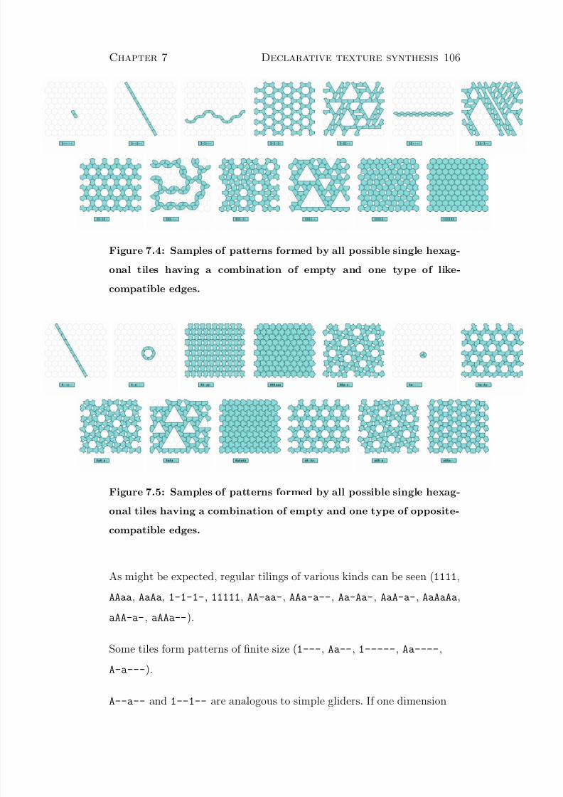
8/20/2019 P. Harrison PhD Thesis
http://slidepdf.com/reader/full/p-harrison-phd-thesis 106/141
Chapter 7 Declarative texture synthesis 106
Figure 7.4: Samples of patterns formed by all possible single hexag-
onal tiles having a combination of empty and one type of like-
compatible edges.
Figure 7.5: Samples of patterns formed by all possible single hexag-
onal tiles having a combination of empty and one type of opposite-
compatible edges.
As might be expected, regular tilings of various kinds can be seen (1111,
AAaa, AaAa, 1-1-1-, 11111, AA-aa-, AAa-a--, Aa-Aa-, AaA-a-, AaAaAa,
aAA-a-, aAAa--).
Some tiles form patterns of finite size (1---, Aa--, 1-----, Aa----,
A-a---).
A--a-- and 1--1-- are analogous to simple gliders. If one dimension

8/20/2019 P. Harrison PhD Thesis
http://slidepdf.com/reader/full/p-harrison-phd-thesis 107/141
Chapter 7 Declarative texture synthesis 107
were to be arbitrarily interpreted as time, these would appear as a single
moving tile.
Various forms of randomness can be seen. This is true randomness, not
Wolfram’s “autoplectic” pseudo-randomness. 11--, and 1-1--- follow
random paths (which may form closed loops). 111--- forms two kinds of
composite units, one with two exposed edges and one with three exposed
edges. A random network results, in which the three-edge units are
nodes and the two-edge units form random paths between these nodes.
111- produces rectangles of random size and shape. 1111-- produces
triangles of random size and orientation. AaAa-- produces triangles of
random size, but of only one orientation. AaAa-- turns out to be related
to the Sierpinski Triangle fractal, as will be seen in the next section.
7.4.2 Further tile sets of interest
Certain tile sets require a great deal of back-tracking on the part of theassembler. These tile sets are often also visually interesting. Two such
sets are shown in Figure 7.6. The set on the left yields patterns with
interesting local mirror symmetries.
Figure 7.6: Tile sets the assembler has difficulty with.
The addition of one or two tiles to AaAa-- (Figure 7.4) yields patterns

8/20/2019 P. Harrison PhD Thesis
http://slidepdf.com/reader/full/p-harrison-phd-thesis 108/141
Chapter 7 Declarative texture synthesis 108
which when finite in size form Sierpinski Triangles (Figure 7.7).
Figure 7.7: Tile sets that yield Sierpinski triangles.
The tile set in Figure 7.8 mimics the structure of DNA.4 The tiles
represent respectively the sugar-phosphate backbone, adenine, thymine,
cytosine, and guanine.
Figure 7.8: Tile set based on DNA.
The tile set on the left in Figure 7.9 is visually reminiscent of a Feynman
diagram containing photons, electrons, and positrons. c--C-- represents
electrons and positrons, and 44---- represents photons. Relaxing the
requirement that the assemblage be connected, and adding a tile for
spontaneous electron-positron creation/annihilation gives rise to
“zero-point fluctuations” (tile set on right).
4This tile set was suggested by Jeff Epler.

8/20/2019 P. Harrison PhD Thesis
http://slidepdf.com/reader/full/p-harrison-phd-thesis 109/141
Chapter 7 Declarative texture synthesis 109
Figure 7.9: Tile sets reminiscent of Feynman diagrams.
Tile sets based on an underlying triangular grid may be simulated using
a hexagonal grid (Figure 7.10). This merely requires that every second
edge be empty.
Figure 7.10: Tile sets based on triangles, simulated with hexagons.
If tiles are decorated by drawing lines connecting different edges, the
results resemble Celtic knot-work (Figure 7.11).

8/20/2019 P. Harrison PhD Thesis
http://slidepdf.com/reader/full/p-harrison-phd-thesis 110/141
Chapter 7 Declarative texture synthesis 110
Figure 7.11: Knot-work patterns. The third pattern consists of a
single loop.
7.4.3 k-morphism and crystallization
Grunbaum and Shephard [1987, pp.46–53] describe a number of tiles
that allow multiple regular tilings. These are called k-morphisms. An
example of this is shown in Figure 7.12. Tile sets were also found that
suggest generalizations of this concept. Figure 7.13 shows a tile set that
yields either regular tiling or a random network pattern. Figure 7.14
shows a tile set with ∞-morphism.
The assembly process (using the algorithm described earlier) shows
behavior reminiscent of crystallization. The assembler initially makes
little progress, but eventually produces a sufficient “seed” from which a
pattern crystallizes outwards rapidly. This might also be considered a
simple form of auto-catalysis.
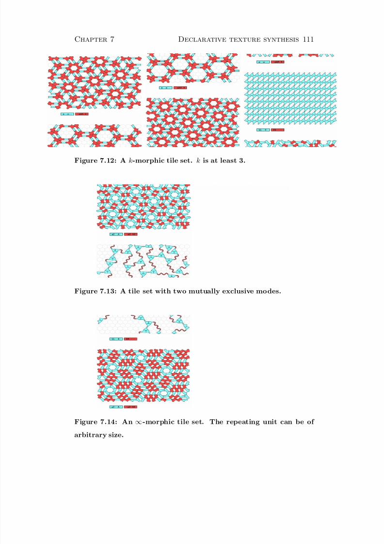
8/20/2019 P. Harrison PhD Thesis
http://slidepdf.com/reader/full/p-harrison-phd-thesis 111/141
Chapter 7 Declarative texture synthesis 111
Figure 7.12: A k-morphic tile set. k is at least 3.
Figure 7.13: A tile set with two mutually exclusive modes.
Figure 7.14: An ∞-morphic tile set. The repeating unit can be of
arbitrary size.

8/20/2019 P. Harrison PhD Thesis
http://slidepdf.com/reader/full/p-harrison-phd-thesis 112/141
Chapter 7 Declarative texture synthesis 112
7.5 Relation to cellular automata
A cellular automaton is a grid of cells in which each cell evolves over
time according to simple local rules. By mapping the time dimension
into a spatial dimension, appropriately shaped tile pieces can be used to
implement cellular automata. This has interesting implications.
7.5.1 Wolfram’s Elementary Cellular Automata
Wolfram’s “Elementary Cellular Automata” [Wolfram, 2002] are
one-dimensional automata in which each cell can be in one of two states,
and in which the state of each cell depends only on the previous state of
that cell and its two immediate neighbours. Such one-dimensional
automata can be mapped into two-dimensional tile sets.
An Elementary Cellular Automaton tile set requires certain crossover
pieces so that tiles implementing the rules of the automaton have accessto all required input edges. The following tiles suffice: a-aC-C, a-bC-D,
b-aD-C, b-bD-D.
A rule tile is required for each possible set of inputs, having three input
edges as follows:
Input Edges
000 cac
001 cad
010 cbc
011 cbd
100 dac
101 dad
110 dbc
111 dbd

8/20/2019 P. Harrison PhD Thesis
http://slidepdf.com/reader/full/p-harrison-phd-thesis 113/141
Chapter 7 Declarative texture synthesis 113
Each rule tile will also have three output edges that represent the state
of the cell, which must be one of:
State Edges0 AAA
1 BBB
The rule number of an Elementary Cellular Automaton when written in
binary gives the mapping from inputs to states. For example, Rule 110
(Figure 7.15) maps to the tile set: a-aC-C/a-bC-D/b-aD-C/b-bD-D/
cacAAA/dacBBB/cbcBBB/dbcBBB/cadAAA/dadBBB/cbdBBB/dbdAAA. Rule
110 has been shown by Matthew Cook to be capable of universal
computation (see Wolfram [2002, pp. 675–689]).
Figure 7.15: Elementary Cellular Automaton Rule 110, as a tile set.
7.5.2 Causality
In the case of tile sets based on cellular automata, a solution may be
found without backtracking by selecting pieces in an order corresponding
to the automata’s time direction. Such tile sets might be described as
causal. Furthermore these tile sets are deterministic, in that the
anti-causal neighbours of a location fully determine which tile must be
placed in it.
That causality is an emergent property of tile sets rather than an
8/20/2019 P. Harrison PhD Thesis
http://slidepdf.com/reader/full/p-harrison-phd-thesis 114/141
Chapter 7 Declarative texture synthesis 114
assumption (as per cellular automata, and simulation of dynamic
systems in general) allows us to think about cases that are “almost”
deterministic-causal. There are two obvious ways to break strict
deterministic causality:
• We might add several tiles that will match a given previous
configuration. The result would be a random cellular automaton.
• We might choose not to include any tile which matches a certain
input configuration. This would forbid any past state that would
lead inevitably to this configuration. The result would be a tile set
that is mostly causal, but with teleological elements.
Combining these two changes would yield a tile set that was “almost”
deterministic causal. This would seem to be an interesting
generalization. It would be interesting to know if teleological effects
would tend to be obscured by random elements on sufficiently large scale
in such a tile set.
The importance of this is not clear, and it is possible that it has no
importance. The most obvious potential application would be in
modelling quantum-scale phenomena. Entanglement, for example, is
straightforward to implement in a near-causal tile-set. The discrete
nature of tile-sets is also appealing at this scale. However it is not
immediately clear how to account for destructive interference of the
wave-function.
7.6 Discussion
A diverse range of patterns were formed from simple tile sets. This is
evidence against Wolfram’s claim that causality is necessary in order for

8/20/2019 P. Harrison PhD Thesis
http://slidepdf.com/reader/full/p-harrison-phd-thesis 115/141
Chapter 7 Declarative texture synthesis 115
interesting patterns to be common. Though some tile sets are
computationally difficult to assemble, many displaying interesting
patterns are not, and these are not strictly those that can be generated in
a causal manner. Causal systems are a class of easy-to-assemble tile sets,
but there are likely to be other classes that yield patterns of comparable
interest with comparable ease of assembly. For example, tile sets whose
assembly by the algorithm described above sometimes requires a large
backtrack, but on average require total backtracking of the order of the
size of the assemblage, can be assembled in linear expected time.
Were the method of texture synthesis described in this chapter applied
to decorating a (real or virtual) object, the nature of the tile-set would
constrain the resulting decoration. One might even need to slightly
redesign the object to suit the tile-set. A certain amount of
back-and-forth would be required. It is the author’s opinion that objects
created using methods that require such back and forth can have greater
aesthetic value than objects created using methods that do not. The
patterns most difficult to work with may also be the ones of greatest
aesthetic value.
There are interesting parallels between tile set patterns, Wolfram’s
cellular automata, and best-fit synthesis, all of which are instances of
Markov Random Field synthesis. We saw in Chapter 3 that a
goodness-of-fit metric based on the thin-tailed Gaussian distribution
produced some characteristic results. Certain features would be repeated
obsessively, in an almost autistic manner, and there were sometimes
regions of “garbage” (this can be seen in Figure 2.6). These features
disappeared when a more robust metric derived from the fat-tailed
Cauchy distribution was used (Figure 3.4). A rule that says two pieces
can not be placed next to each other unless they exactly match is also a
kind of “thin tailed” criterion: the tail is so thin that it is zero! The
rules of a Wolfram-style cellular automaton are another instance of this

8/20/2019 P. Harrison PhD Thesis
http://slidepdf.com/reader/full/p-harrison-phd-thesis 116/141
Chapter 7 Declarative texture synthesis 116
– a particular rule either matches or it does not. Do we see these same
characteristic patterns in cellular automata and tile set patterns? Yes.
Excessive repetition is what Wolfram would call a glider. Indeed, in
Figure 2.6, E3 displays features that are very clearly gliders (interpreting
movement down the page as progression in time). And “garbage” is
what Wolfram would call autoplectic randomness.
A criticism of Wolfram’s work can be made on this basis. It is Wolfram’s
thesis that these kinds of features are seen in all forms of computation,
and irrespective of the complexity of the underlying rules. However,
Wolfram only studies discrete rules in detail, and these may all be
characterized as “very thin tailed”. More forgiving rules, such as the
Cauchy-based metric introduced in Chapter 3 do not show these
characteristics. “Thin-tailed” rules will tend to obsessively rely on only a
small portion of the rule-set5, so the size of the total rule set may not
have much effect on the result. “Fat-tailed” rules, in which a rule is still
applicable even if some criteria do not match exactly, will give rise to a
more representative sampling of the total rule set, and may be capable of
a richer set of behaviors.
For example, compare the best fit synthesis results for test image E3
using a Gaussian and Cauchy metric (Figure 7.16). With the heavier
tailed Cauchy metric, the repeating “glider” patterns are reduced.
5In best-fit synthesis, the rule-set is derived from the contents of the texture image.
Its complexity is proportional to the size of this image.

8/20/2019 P. Harrison PhD Thesis
http://slidepdf.com/reader/full/p-harrison-phd-thesis 117/141
Chapter 7 Declarative texture synthesis 117
(a) (b)
Figure 7.16: Test image E3 synthesized using Garber’s method. (a)
original metric, (b) Cauchy metric (σ = 15).
Interestingly, a causal relation between elements does not seem necessary
in order to produce this “autistic” behavior. The tile set patterns of this
chapter also contain repeating “gliders”, and multiple modes
(k-morphism) which lock themselves in such that a pattern can not be
extended to form a transition to a different mode. The best-fit variant
described in Chapter 3 also approximates acausality by choosing pixels
in random order and by refining early chosen pixel values on the basis of
later chosen ones, yet still produces obsessive repetitions when the
Gaussian derived metric is used.

8/20/2019 P. Harrison PhD Thesis
http://slidepdf.com/reader/full/p-harrison-phd-thesis 118/141
Chapter 8
Conclusion and future work
In the introduction, three texture operations were identified: texture
synthesis, texture transfer, and plausible restoration. This dissertation
has presented several different approaches to performing these
operations:
• A variant of the best-fit method that is fast and flexible, capable of
all three operations (Chapter 3).
• A fast patchwork synthesis method, capable of texture synthesis
and transfer (Chapter 5).
• A method based on texture modelling, capable of plausible
restoration of both missing areas and noise corrupted images(Chapter 6).
These represent different trade-offs between speed, quality, and
generality. In particular, the best-fit variant described in Chapter 3
represents a practical approach to these operations in a wide range of
circumstances, and is in current use as a GIMP plug-in.
118

8/20/2019 P. Harrison PhD Thesis
http://slidepdf.com/reader/full/p-harrison-phd-thesis 119/141
Chapter 8 Conclusion and future work 119
Some theoretical aspects of texture synthesis were also explored using
tile patterns (Chapter 7). This served to place methods of performing
the texture operations presented here and elsewhere in context.
An image, even if damaged, contains a great deal of information about
its texture. As the methods of Chapters 3 and 6 demonstrated, this
information may be extracted from the image and used to repair or alter
it. We need not pre-program into methods of performing texture
operations specific information about the types of features found in
images (such as that they might contain sharp edges, or spot and edge
features of different scales), as this information is already present in the
image. Indeed to specify these things a priori may limit the range of
images a method can successfully operate on.
Methods such as the plausible restoration method of Chapter 6 may
eventually out-perform the best-fit method and variants, as such
methods are capable not just of copying existing areas of texture but
inventing new plausible instances of that texture based on an inferredmodel of the texture. For example, such methods may extrapolate pixel
values outside of the bounds seen in the available texture sample (see
Figure 6.5). A major weakness with the method presented in Chapter 6,
however, is that it is one of finding a unique optimum. The best-fit
methods, by contrast, sample from a field of possibilities. The method of
Chapter 6 can therefore reconstruct smooth curves, but not replicate the
roughness of the original texture.
To remove this weakness, the merit function (Equation 6.4) would need
to be replaced by an explicit probability density function, and random
samples produced based on that function. A random sample might be
produced from such a probability density function using the
Metropolis-Hastings algorithm (see Section 2.2.2). Such an extension
would also allow the method of Chapter 6 to be applied to texture

8/20/2019 P. Harrison PhD Thesis
http://slidepdf.com/reader/full/p-harrison-phd-thesis 120/141
Chapter 8 Conclusion and future work 120
synthesis and texture transfer. However, given the large number of
parameters involved (one parameter per pixel of the image, plus the
parameters of the model), a naive application of this algorithm will take
an unreasonable number of iterations to converge. Finding a variant of
the Metropolis-Hastings algorithm that converges quickly is an open
problem.
An interesting feature of the texture operations identified in the
introduction is that they can bypass modelling. To predict the value of
some unknown data we normally select a model based on the data we
have available (induction) and use this model to predict the unknown
data (deduction). There is a problem, however, with deciding exactly
which model to use. If the most likely model is chosen (Maximum
Likelihood), we have ignored the possibility that the data was a less
likely product of a slightly less likely model. The Maximum Likelihood
model will tend to over-fit the data. Statisticians avoid over-fitting by
using “unbiased” estimators of model parameters. An unbiased
estimator is a means of estimating a parameter such that the average
expected value of the estimator, when applied to a sample of any size, is
equal to the true value of the parameter [McGee, 1971, pp.99–100]. An
unbiased estimate may be found for any single parameter in a model,
but combining these estimates into a full model does not produce an
unbiased model. For example, if a texture sample were insufficiently
large to allow a decision between two different possible models of
texture, a model composed of unbiased parameters
might—incorrectly—allow a mixture of the two possible textures in a
single image. This problem will occur in any method that tries to use a
single model to characterize the field of all possible models.
However, when performing the texture operations, we need not settle on
a specific model. The output of the texture operations is a random
sample from the field of all possible results. Methods of performing
8/20/2019 P. Harrison PhD Thesis
http://slidepdf.com/reader/full/p-harrison-phd-thesis 121/141
Chapter 8 Conclusion and future work 121
texture operations may choose a model at random (conformant to the
probability distribution of models given the input data), or omit
modelling entirely. The best-fit method omits modelling, producing new
samples directly from the sample given.1 If the method of Chapter 6
were extended to perform sampling, as described above, the sample
produced would have an associated randomly sampled model.
Beyond sampling from the field of possible images, we may wish to
characterize the full field. This would be useful where we need to be sure
that what we are reconstructing is really there, and not just a plausible
confabulation (for example, in medical or military applications). We
may wish to find the average image, or measure the amount of possible
variation in a particular region, or calculate some other relevant
statistics. For example, in Figure 6.3, some fine texturing in the hat was
lost. The values of pixels in the hat in the image of maximum likelihood
happen to lie at the boundary of their allowed ranges, and are not
representative of the field of possibilities. An average of the field would
be more representative, and would preserve this fine texturing without
inventing new details.
In conclusion, significant progress has been made in this dissertation
towards the ideal of an all-purpose texture tool, and has also mapped
out some fundamental challenges that must be taken into account when
creating such tools. Ongoing development of more powerful tools will
provide a richer environment of interactions between artists and
designers and the objects they create, helping better express both the
intentions of artists and designers and the underlying logic of the
textures with which they work.
1To produce a truly random sample, the best-fit method would need to examinepreviously synthesized areas of the output in addition to the input. The plausiblerestoration method described by Drori et al. [2003] does this.

8/20/2019 P. Harrison PhD Thesis
http://slidepdf.com/reader/full/p-harrison-phd-thesis 122/141
Chapter 8 Conclusion and future work 122

8/20/2019 P. Harrison PhD Thesis
http://slidepdf.com/reader/full/p-harrison-phd-thesis 123/141
Appendix A
Test suites
In this dissertation, various texture operations needed to be tested. For
this purpose, a test-suite of images was selected. Also, images suitable
for texture transfer were selected.
123
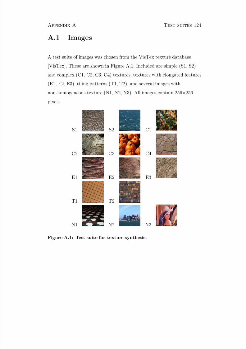
8/20/2019 P. Harrison PhD Thesis
http://slidepdf.com/reader/full/p-harrison-phd-thesis 124/141
Appendix A Test suites 124
A.1 Images
A test suite of images was chosen from the VisTex texture database
[VisTex]. These are shown in Figure A.1. Included are simple (S1, S2)
and complex (C1, C2, C3, C4) textures, textures with elongated features
(E1, E2, E3), tiling patterns (T1, T2), and several images with
non-homogeneous texture (N1, N2, N3). All images contain 256×256
pixels.
S1 S2 C1
C2 C3 C4
E1 E2 E3
T1 T2
N1 N2 N3
Figure A.1: Test suite for texture synthesis.

8/20/2019 P. Harrison PhD Thesis
http://slidepdf.com/reader/full/p-harrison-phd-thesis 125/141
Appendix A Test suites 125
A.2 Texture transfer
Test images for texture transfer were also selected. The two textures
(Figure A.2a) were taken from the VisTex database [VisTex] and are
both 512×512 pixels in size. The pattern images (Figure A.2b) were
taken with a digital camera, and are 825×630 and 548×804 pixels in size
respectively.
(a) S1 S2
(b) I1 I2
Figure A.2: Texture transfer test suite: (a) texture samples, (b)
images.

8/20/2019 P. Harrison PhD Thesis
http://slidepdf.com/reader/full/p-harrison-phd-thesis 126/141
Appendix B
Paper presented at
WSCG-2001
The following paper was presented at WSCG-2001, a computer graphics
conference held at the University of West Bohemia in the Czech
Republic. It describes an early and overly complicated attempt at
tackling the problems addressed in Chapter 3.
Google Scholar1 lists 22 citations of this paper by other authors.
1http://scholar.google.com/
126

8/20/2019 P. Harrison PhD Thesis
http://slidepdf.com/reader/full/p-harrison-phd-thesis 127/141
Appendix B Paper presented at WSCG-2001127
A NON-HIERARCHICAL PROCEDURE FOR
RE-SYNTHESIS OF COMPLEX TEXTURES
Paul Harrison
School of Computer Science and Software EngineeringMonash University
Wellington Rd.Clayton, 3800
Melbourne, Australia
ABSTRACT
A procedure is described for synthesizing an image with the same texture as a given input image.To achieve this, the output image is built up by successively adding pixels selected from the inputimage. Pixels are chosen by searching the input image for patches that closely match pixels alreadypresent in the output image. It is shown that the accurate reproduction of features in the inputtexture depends on the order in which pixels are added to the output image. A procedure forselecting an ordering which transfers large complex features of the input to the output image isdescribed. This procedure is capable of reproducing large features even if only the interactions of nearby pixels are considered. The procedure can be altered to allow specification of the placementof particular features in the output texture. Several applications of this are described.
Keywords: texture synthesis, image manipulation
1 INTRODUCTION
The texture of an image might be defined broadlyas the interrelationships between pixels in thatimage. The ability to analyse and manipulateimage texture has a number of interesting appli-cations. The simplest application is to create anew image with the same texture but of differentsize and shape to a sample image. Seamless edit-ing of images is also a possibility. For example anobject could be removed from an image by syn-thesizing a new section of the background texture
over the top of it. These applications all rely onthe ability to re-synthesize a sample texture to fita variety of constraints.
A number of texture re-synthesis methods aredescribed in the literature. One approach isbased on searching for specific features in textures[Heege95] [Bonet97] [Porti99]. In these meth-ods, the input image is decomposed into a set of features. Statistics about these features are col-lected, and used to synthesize a new image. Oneproblem with these methods is that they can only
recognize a set of features which have been speci-fied in advance. While the results can be impres-sive, it is difficult to devise a generic feature setthat can be used to describe all textures.
Another approach to the texture re-synthesisproblem is to analyse and reproduce interactionsbetween individual pixels [Monne81] [Gagal90].Methods based on this approach define a func-tion describing a pixel in terms of its neighboursand a random element. This function is used togenerate a new image, pixel by pixel.
Recently, a new pixel-based technique has beendeveloped based on best-fit searching. Garber[Garbe81] and Efros and Leung [Efros99] inde-pendently developed this approach, in which eachpixel is selected by searching the input image fora patch of pixels closely matching nearby pixelsalready present in the output image. This resultsin an output image pieced together from smallparts of the input image. Using this technique,textures can be synthesized in which the relation-ships between neighbouring pixels are extremely

8/20/2019 P. Harrison PhD Thesis
http://slidepdf.com/reader/full/p-harrison-phd-thesis 128/141
Appendix B Paper presented at WSCG-2001128
ΩI
: The set of pixel locations inthe input image.
I (s), s ∈ ΩI : The pixel in the input imageat location s.
ΩO : The set of locations contain-ing pixels in the output im-age.
O(s), s ∈ ΩO : The pixel in the output im-age at location s.
L(s), s ∈ ΩO : The location of the pixel inthe input image that is inthe output image at locations.
ΩK : The set of offsets consideredwhen calculating the simi-larity of two texture patches.
K (u), u ∈ ΩK : Weighting given to a partic-ular offset u.
A(s), s ∈ ΩI
B(s), s ∈ ΩO : Two uniformly randomfunctions.
Table 1: Table of symbols.
complex.
Efros and Leung report that for good results thesize of the patch searched for in the input im-age should correspond to the size of the largest
feature in the texture. To allow larger features,Wei and Levoy [Wei00] propose a hybrid of thefeature-based and best-fit techniques that gener-ates the output in a pyramid of successively finerresolutions.
This paper presents a refinement of the pixel-based best-fit re-synthesis procedures introducedby Garber [Garbe81] and Efros and Leung[Efros99]. The most important change is to theselection of the order in which pixels are added tothe output image. This order is selected to allowreproduction of features larger than the size of the patches searched for in the input image. Theprocedure avoids decomposing the input imageinto a predefined feature set, and can thereforere-synthesize a wide range of textures. An ex-tension to this procedure is presented that allowsspecification of the layout of different regions of texture in the output image.
2 RE-SYNTHESIS PROCEDURE
The procedure described in this paper takes asinput an image containing a sample of a textureand produces another image with the same tex-ture.
The procedure has two stages. In the first stage,pixel interrelationships in the input image areanalysed. The extent to which the value of eachpixel constrains the values that can be taken byneighbouring pixels is determined. The reasonsfor doing this are discussed in section 2.1 andthe calculations necessary are described in sec-tion 2.2.
In the second stage, pixels are added to the ini-tially blank output image until all locations havebeen filled. The order in which pixels are addedis chosen to facilitate faithful reproduction of the texture of the input image, using the resultsfrom the first stage, as described in sections 2.1and 2.2.1. Section 2.2.1 also describes the ini-
tialization of this stage in terms of choice of thelocations and values of seed pixels.
To add a pixel to the output image at a partic-ular location, the surrounding pixels which havealready been added to the output image are ex-amined. The closest match to these pixels is lo-cated in the input image, and the correspondingpixel from the input image is inserted in the out-put. This is described below and in section 2.2.2.
Symbols used in this paper are listed in Table 1.
Colours are stored as RGB values. To compareindividual pixels, the sum of the absolute values
of the differences in each colour component wasused:
d((r1, g1, b1), (r2, g2, b2)) =|r2 − r1| + |g2 − g1| + |b2 − b1|
(1)
To measure how closely patches from the inputimage match a patch in the output image, a dis-tance function can be used. The distance func-tion used in this paper is a weighted Manhattan(city block) distance function. To allow synthe-sis of textures with a random element, the dis-tance function contains a small random compo-nent with weight specified by the parameter ε:
D(s, t) = ε |A(s) −B(t)|+
u∈ΩK ,t+u∈ΩOK (u)d(I (s + u), O(t + u))
(2)
The Manhattan distance was chosen over themore commonly used Euclidean distance as it ismore forgiving of outliers. I.e. a good match inmost pixels in the patch will not be negated by apoor match in one or two pixels.

8/20/2019 P. Harrison PhD Thesis
http://slidepdf.com/reader/full/p-harrison-phd-thesis 129/141
Appendix B Paper presented at WSCG-2001129
Figure 1: Barcode texture.
For each location t in the output image, a pixelI (s) from the input image is chosen. The locations in the input image is selected to minimize thedistance D(s, t) as given in Eq. 2.
2.1 Ordering of pixel insertion
This section discusses the order in which pixelsare added to the output image in the second stageof the procedure. As will be demonstrated, cer-tain features such as branching patterns are onlyreproduced correctly in the output image if theplacement of pixels proceeds in a particular or-der.
Consider the values a particular pixel in a tex-tural image could take. The pixel value must beconsistent with the values of all other pixels inthe image. These other pixels may be said toconstrain the values the selected pixel can take.
An important property of these constraints is that
the constraint imposed by a distant pixel in somedirection may also be provided by a closer pixelin the same direction. In general, most of theconstraint will be imposed by nearby pixels. Forexample, in Fig. 1 the constraint imposed by pix-els far above or below a given pixel will also beprovided by pixels a small distance above or be-low that pixel. This kind of relationship may bedirectional. In Fig. 1 it applies vertically but nothorizontally.
These constraints can be thought of in terms of information theory [Blahu87]. Without any priorknowledge, a pixel is equally likely to take anyvalue, and this requires a certain number of bits
to encode. If its neighbours impose constraints onthe values it can take, it will require (on average)less bits to encode. The average number of bitsrequired to encode some information is referredto as its entropy [Blahu87, pp. 55]. Entropy cantherefore be used to measure the constraints im-posed on a pixel.
The pixel selection procedure is based on a searchfor patches of pixels in the input image thatmatch those already placed in the output. Thesepatches must cover enough pixels to capture all
(a) (b)
1 1 11 1 1 1 11 1 P 1 11 1 1 1 1
1 1 1
(c) (d)
(e) (f)
Figure 2: Textures generated using differ-ent orders of pixel insertion.
Input image (a), weighting of the distance function
K (u) used about the center pixel P (b), and the out-
put from raster scans proceeding from top to bottom
(c), bottom to top (d), left to right (e), and right to
left (f).
the constraints on each location, or the texturewill not be reproduced correctly. However, if thepatch size is too large, there will be less chance
of finding good matches in the input image. It istherefore desirable to choose an order to add pix-els to the output image in which the constraintsimposed on each location are captured by a smallneighbourhood of pixels.
One order that can be used to add pixels is araster scan. Fig. 2 shows images generated usingraster scans in different directions. The lichentexture being synthesized has a complex branch-ing pattern. As can be seen, the scan that pro-ceeds from bottom to top (Fig. 2d) reproducesthis pattern the most accurately.
The other raster scans in Fig. 2 have various prob-
lems. The top to bottom scan (Fig. 2c) producesanomalous dark blotches, and the lichen in thesideways scans (Fig. 2e and 2f) have branches onone side only.
These artifacts can be explained by consideringhow the pixels constrain one another. The con-straint imposed on a given pixel by the pixels im-mediately below it is almost the same as the con-straint imposed by all pixels below it. This is nottrue of pixels above or to either side of that pixel.The bottom-to-top raster scan therefore produces
8/20/2019 P. Harrison PhD Thesis
http://slidepdf.com/reader/full/p-harrison-phd-thesis 130/141
Appendix B Paper presented at WSCG-2001130
a better result than the others tested.
To utilize these types of constraint, the re-synthesis procedure assigns a priority to each lo-cation in the output image. Highest priority isgiven to locations which are highly constrainedby neighbouring pixels that have already beenadded. Then the following procedure is followed:
While there are still empty locations in
the output image:
• Find the empty location with the
highest priority.
• Choose a pixel from the input image
to place in that location.
• Update priorities of empty
neighbouring locations based on the
new pixel value.
A system for assigning priorities needs to be cho-sen. A simple prioritization scheme estimatesthe entropy of each unfilled location given itsnearby neighbours, and gives higher priority tolocations with lower entropy. The problem withthis scheme is that there may be some areas of atexture in which nearby pixels tightly constraineach other, and others where there is less con-straint and pixel values are more random. Theareas with tight constraints will always be givenhigher priorities and therefore be disproportion-ately represented in the output image.
The approach taken in this paper is to define anormalized weighting W (s, u). This weighting in-dicates the relative amount of information a pixelI (s) gives about each of its neighbours I (s + u).To ensure no part of the image is given an advan-tage over another part, this weighting is definedso that it sums to unity for each pixel I (s). Thepriority of each empty location in the output canthen be defined as a sum of the weightings fromneighbouring pixels.
2.2 Analysing interactions between
neighbouring pixels
Weightings are needed to prioritize the order inwhich pixels are inserted. They are also needed inthe distance function used to select these pixels.To create these weightings, interactions betweenneighbouring pixels in the input image are anal-ysed. The calculation of these weightings is thefirst stage of the synthesis procedure. For pur-poses of computational simplicity, the effect of each neighbour on a location is assumed to beindependent of the effects of other neighbours.The interactions between constraints of differentneighbours on a location are neglected.
To compute the weightings, the amount of in-formation every pixel provides about each of itsnear neighbours first needs to be estimated. Theneighbours being considered are those whose off-set from the central pixel is a member of the set of offsets ΩK used to calculate the distance functionD(s, t) (Eq. 2).
These amounts of information may be measuredby considering each offset u ∈ ΩK in turn. Foreach offset, the number of bits of informationG(s, u) provided by each pixel in the input im-age I (s) about the pixel offset from it I (s + u) isestimated, as explained below.
Offset pixels I (s + u) are grouped into sets based
on the value of the corresponding pixel I (s).Within each set, the pixels will have a distribu-tion of values. These values are modelled as be-ing normally distributed in each colour compo-nent (red, green and blue), and the parameters of these distributions are estimated. This is used tocalculate the number of bits required to encodepixels of each set.
To distribute the pixels I (s + u) into sets, theyare classified by the most significant m bits of the red, green and blue components of I (s). Thevalue of m should be chosen so that the sets areneither so small that an accurate estimate of themean and standard deviation is impossible, nor
so large that most of the information from I (s) isdiscarded.
If it is assumed that all the pixels in aset come from the same distribution, stan-dard deviations calculated from the sets canbe used to describe individual pixels in thosesets. This gives standard deviations for eachpixel at each offset for each colour component:σr(s, u), σg(s, u), σb(s, u).
These standard deviations can be used to calcu-late the entropy of each pixel I (s + u) given I (s).The average number of bits required to store anormally distributed variable with standard de-viation σ , to an accuracy of ±1
2 , is:
1
2 log2(2π) +
1
2 l n 2 + log2 σ (3)
Summing this for each colour component givesthe entropy of the pixel I (s + u) given I (s):
H (s, u) = 3
2 log2(2π) + 3
2ln2
+log2 σr(s, u)σg(s, u)σb(s, u) (4)
8/20/2019 P. Harrison PhD Thesis
http://slidepdf.com/reader/full/p-harrison-phd-thesis 131/141
Appendix B Paper presented at WSCG-2001131
Performing the same calculation without splittingthe image into sets gives the entropy of pixels inthe image independent of any of their neighbours,H image.
The number of bits given by a pixel I (s) aboutanother pixel offset from it I (s + u) can then befound by subtracting the entropy of I (s+u) givenI (s) from the entropy of pixels in the image if nothing is known about their neighbours. Callthis value G(s, u), where:
G(s, u) = H image −H (s,u) (5)
2.2.1 Prioritization weighting
A normalized weighting W (s, u) suitable for pri-oritizing the order in which pixels are added tothe output image can be defined from G(s, u) :
W (s, u) = G(s, u)−v∈ΩK
G(s, v) (6)
The priorities of unfilled locations in the outputimage may be defined from W (s, u) :
P (s) =
u∈ΩK ,s+u∈ΩO
W (L(s + u),−u) (7)
Additionally, locations near the edge of the imagehave their priorities adjusted as if the positionsbeyond the edge of the image were already filledby pixels having average properties (i.e. withweights W (s, u) averaged over all s). These lo-cations then act as starting positions for fillingthe output image. The value of the first pixeladded, having no neighbours, is chosen at ran-dom from the input image (on the basis of therandom component of the distance function).
2.2.2 Distance function weighting
The distance function D(s, t) (Eq. 2) used to se-lect pixels also requires a set of weightings. Tomake best use of the input image, these weight-ings should reflect the degree to which each neigh-bour constrains the value of the pixel.
The entropy of a normally distributed randomvariable, such as one of the color components of
a pixel, is the logarithm to base two of its stan-dard deviation, to within a constant (see Eq. 3).This means that for each time a constraint on aparticular location halves the standard deviationof possible values of one color component of thatlocation, one more bit of information about thelocation becomes known. In light of this relation-ship, the weighting given to a neighbour might bedoubled for every bit it gives about a location.
The weighting system used in the distance func-tion was chosen to satisfy this constraint:
K (u) = 2G(−u) (8)
where G(u) is the average value of the weightingsG(s, u) for a particular offset u.
2.3 Results of the procedure
Example results from the procedure are shown inFig. 3. A seven by seven neighbourhood of pix-els (ΩK = [−3, 3] × [−3, 3]) was used to generatethese images.
The images in Fig. 3 required an average of fourand a half minutes and six and a half megabytesof memory to produce on a 300Mhz Pentium II.
The time taken by the procedure increases ap-proximately linearly with the size of the inputimage, and can be extremely slow for large inputimages.
Less successful results are shown in Fig. 4. Inparticular the procedure is very sensitive to fea-tures that only appear at the edge of the inputimage. In this case the output tends to containartifacts such as repeating patterns. Also, as canbe seen in Fig. 4b, the procedure does not rec-ognize regularly spaced components of a texturesuch as tiles.
3 SPECIFICATION OF THE
PLACEMENT OF TEXTUREREGIONS
Some textures contain several regions, with prop-erties that differ from one region to another. Asimple extension to the distance function used toselect pixels gives a means of specifying the layoutof these regions in the output image. This exten-sion requires the definition of two new images,one which maps regions in the input, J (s), andone which specifies corresponding regions in theoutput, Q(t). It also requires weightings, L(u),

8/20/2019 P. Harrison PhD Thesis
http://slidepdf.com/reader/full/p-harrison-phd-thesis 132/141
Appendix B Paper presented at WSCG-2001132
Figure 3: Sample results.The output of the procedure is shown below each in-
put image.
which represent the relative importance of pix-els from the input map in determining the valueof their surrounding pixels in the input image.These are chosen using the same method as thatused to choose K (u). Then a new distance func-tion is used in place of Eq. 2:
D(s, t) = ε |A(s) −B(t)| +u∈ΩK ,t+u∈ΩO
K (u)d(I (s + u), O(t + u))+
L(u)d(J (s + u), Q(t + u))(9)
(a) (b)
An implementation of the procedure can be ob-tained from http://www.csse.monash.edu.au/
~pfh/resynthesizer/
Figure 4: Some failures.
3.1 Results of the extended procedure
An example of the use of the extended synthe-sis procedure is shown in Fig. 5. The textureused was a photograph of clouds (Fig. 5b). Amap of this texture was created showing regionsof cloud and blue sky (Fig. 5a). Another map, of a checkerboard pattern, was used as the outputmap (Fig. 5c). The result of applying the proce-dure to these three images is shown in Fig. 5d.
Texture re-synthesis has been previously appliedto the removal of objects on a homogeneous back-ground by synthesizing a new section of thatbackground [Igehy97] [Efros99]. The ability toconstrain placement of texture regions allows syn-thesis of a new background to replace an object,
even if the background is non-homogeneous. Anexample of this is shown in Fig. 6. Fig. 6a showsa picture of a donkey standing in a field. In thispicture, the field is not homogeneous because of perspective expansion. A feature map of the im-age (Fig. 6b) was constructed with parts of theimage equidistant from the camera having thesame value. A new section of the background wasthen synthesized to replace the donkey, using therest of the background as input texture. The newsection was constrained to join with the existingbackground and to follow the feature map. The

8/20/2019 P. Harrison PhD Thesis
http://slidepdf.com/reader/full/p-harrison-phd-thesis 133/141
Appendix B Paper presented at WSCG-2001133
(a) (b)
(c) (d)
Figure 5: Constraining a cloud texture to acheckerboard pattern.
Input map (a), input texture (b), output map (c),
and output of the extended synthesis procedure (d).
(a)
(b)
(c)
Figure 6: Example of object removal.Original image (from [Igehy97]) (a), map (b), and
image with object removed (c).
result is shown in Fig. 6c.
4 CONCLUSION AND FUTURE
WORK
A procedure has been described for synthesizingan image of arbitrary size with the same textureas that of a sample input image. The procedureis capable of reproducing large features from thisinput image, even though it only examines inter-actions between pixels that are close neighbours.Significantly, the procedure does not have anypreconceived notion of what features to expectin the input texture.
A simple extension to this procedure allows fea-
ture placement in the new image to be con-strained. It is effectively a generic filter, in thatwhen given an example of a change to one im-age it can reproduce the same change in anotherimage.
Future work on the procedure described herecould refine the distance function to considermatches that have similar structure even if theyare slightly lighter or darker or have a differenthue. It could also be extended to work on non-flat geometries, to allow synthesis of textures cov-ering three-dimensional ob jects. It might also beapplied to three dimensions to manipulate anima-tions or solid textures, or to one dimension as asound synthesis technique.
ACKNOWLEDGEMENTS
I thank my P.h.D. supervisor, Dr. Alan Dorin,for his patience and for many helpful suggestions.I also thank Homan Igehy and Lucas Pereira forthe use of one of their images in this paper.
REFERENCES
[Blahu87] R. E. Blahut. Principles and Practice
of Information Theory . Addison-Wesley,1987.
[Bonet97] J. S. De Bonet. Multiresolution sam-pling procedure for analysis and synthesisof texture images. In Proceedings of SIG-
GRAPH 1997 , pages 361–368, 1997.
[Efros99] A. A. Efros and T. K. Leung. Texturesynthesis by non-parametric sampling. InProceedings of the 7th IEEE International
Conference on Computer Vision , pages1033–1038, 1999.
[Gagal90] A. Gagalowicz and S. De Ma. Sequen-tial synthesis of natural textures. In Se-
lected Papers on Digital Image Processing ,
8/20/2019 P. Harrison PhD Thesis
http://slidepdf.com/reader/full/p-harrison-phd-thesis 134/141
Appendix B Paper presented at WSCG-2001134
pages 184–210. SPIE Optical EngineeringPress, 1990.
[Garbe81] D. Garber. Computational Models for
Texture Analysis and Texture Synthesis .PhD thesis, University of Southern Cali-fornia, 1981.
[Heege95] D. J. Heeger and J. R. Bergen.Pyramid-based texture analysis/synthesis.In Proceedings of SIGGRAPH 1995 , pages229–238, 1995.
[Igehy97] H. Igehy and L. Pereira. Image replace-ment through texture synthesis. In Pro-
ceedings of the 1997 IEEE International
Conference on Image Processing , 1997.
Available: http://graphics.stanford.edu/papers/texture_replace/
(Accessed: 2000, September 7).
[Monne81] J. Monne, F. Schmitt, and D. Massa-loux. Bidimensional texture synthesis byMarkov chains. Computer Graphics and
Image Processing , 17:1–23, 1981.
[Porti99] J. Portilla and E. P. Simoncelli. Tex-ture modeling and synthesis using jo-ing statistics of complex wavelet coef-ficients. In Proceedings of the IEEE
Workshop on Statistical and Computa-
tional Theories of Vision , 1999. Avail-able: http://www.cis.ohio-state.edu/
~szhu/SCTV99.html (Accessed: 2000,September 7).
[Wei00] L. Wei and M. Levoy. Fast texture syn-thesis using tree-structured vector quan-tization. In Proceedings of SIGGRAPH
2000 , 2000. Available: http://graphics.stanford.edu/projects/texture/ (Ac-cessed: 2000, September 7).

8/20/2019 P. Harrison PhD Thesis
http://slidepdf.com/reader/full/p-harrison-phd-thesis 135/141
Bibliography
M. Ashikhmin. Synthesizing natural textures. In Proceedings of the
ACM Symposium on Interactive 3D Graphics , pages 217–226. ACM
Press, 2001.
M. Ashikhmin. Fast texture transfer. IEEE Computer Graphics and
Applications , 23(4):38–43, 2003.
J. R. Bergen and E. H. Adelson. Early vision and texture perception.
Nature , 333:363–364, May 1988.
V. Bhaskaran and K. Konstantinides. Image and Video Compression Standards . Kluwer Academic Publishers, 1995.
C. Blakemore and G. F. Cooper. Development of the brain depends on
the visual environment. Nature , 228:477–478, 1970.
S. Brin. Near neighbour search in large metric spaces. In Proceedings of
the 21st International Conference on Very Large Data Bases , pages
574–584, Zurich, Switzerland, 1995. Morgan Kaufmann Publishers.
R. Chellappa and R. L. Kashyap. Texture synthesis using 2-d noncausal
autoregressive models. IEEE Transactions on Acoustics, Speech, and
Signal Processing , 33(1):194–203, February 1985.
M. F. Cohen, J. Shade, S. Hiller, and O. Deussen. Wang tiles for image
and texture generation. In Proceedings of SIGGRAPH 2003 , pages
287–294. ACM Press, 2003.
135

8/20/2019 P. Harrison PhD Thesis
http://slidepdf.com/reader/full/p-harrison-phd-thesis 136/141
BIBLIOGRAPHY 136
P. L. Combettes. Image restoration subject to a total variation
constraint. IEEE Transactions on Image Processing , 13(9):1213–1222,
2004.
A. Criminisi, P. Perez, and K. Toyama. Region filling and object
removal by examplar-based image inpainting. Technical Report
MSR-TR-2003-84, Microsoft Corporation, 2003.
K. Culik. An aperiodic set of 13 wang tiles. Discrete Mathematics , 160:
245–251, 1996.
J. S. DeBonet. Multiresolution sampling procedure for analysis and
synthesis of texture images. In Proceedings of SIGGRAPH 1997 , pages
361–368. ACM Press, 1997.
I. Drori, D. Cohen-Or, and H. Yeshurun. Fragment-based image
completion. In Proceedings of SIGGRAPH 2003 , pages 303–312. ACM
Press, 2003.
D. S. Ebert, F. K. Musgrave, D. Peachy, K. Perlin, and S. Worley.
Texturing and Modelling: a procedural approach . Academic Press Inc.,
1994.
A. A. Efros and W. T. Freeman. Image quilting for texture synthesis
and transfer. In Proceedings of SIGGRAPH 2001, pages 341–346.
ACM Press, 2001.
A. A. Efros and T. K. Leung. Texture synthesis by non-parametric
sampling. In Proceedings of the 7th IEEE International Conference on
Computer Vision , pages 1033–1038. IEEE, 1999.
C. Fearnley. Where have all the Textures gone? John McIndoe Ltd, 1975.
J. H. Friedman. An algorithm for finding best matches in logarithmic
expected time. ACM Transactions on Mathematical Software , 3(3):
209–226, September 1977.

8/20/2019 P. Harrison PhD Thesis
http://slidepdf.com/reader/full/p-harrison-phd-thesis 137/141
BIBLIOGRAPHY 137
D. Garber. Computational Models for Texture Analysis and Texture
Synthesis . PhD thesis, University of Southern California, 1981.
M. Ghazel, G. H. Freeman, and E. R. Vrscay. Fractal image denoising.IEEE Transactions on Image Processing , 12(12):1560–1578, 2003.
G. Gilboa, N. Sochen, and Y. Y. Zeevi. Forward-and-backward diffusion
processes for adaptive image enhancement and denoising. IEEE
Transactions on Image Processing , 11(7):689–703, 2002.
B. Grunbaum and G. C. Shephard. Tilings and Patterns . W. H.
Freeman and Company, 1987.
P. F. Harrison. A non-hierarchical procedure for re-synthesis of complex
textures. In WSCG’2001, pages 190–197, Plzen, Czech Republic, 2001.
University of West Bohemia.
D. J. Heeger and J. R. Bergen. Pyramid-based texture
analysis/synthesis. In Proceedings of SIGGRAPH 1995 , pages
229–238. ACM Press, 1995.
C. W. Helstrom. Image restoration by the method of least squares. In
Selected Papers on Digital Image Processing , pages 619–625. SPIE
Optical Engineering Press, 1990.
A. Hertzmann, C. E. Jacobs, N. Oliver, B. Curless, and D. H. Salesin.
Image analogies. In Proceedings of SIGGRAPH 2001. ACM Press,
2001. Available: http://mrl.nyu.edu/projects/image-analogies/
(Accessed: 2002, May 31).
D. H. Hubel and T. N. Wiesel. Receptive fields, binocular interaction
and functional architecture in the cat’s visual cortex. Journal of
Physiology , 160:106–154, 1962.
H. Igehy and L. Pereira. Image replacement through texture synthesis.
In Proceedings of the 1997 IEEE International Conference on Image

8/20/2019 P. Harrison PhD Thesis
http://slidepdf.com/reader/full/p-harrison-phd-thesis 138/141
BIBLIOGRAPHY 138
Processing . IEEE, 1997. Available:
http://graphics.stanford.edu/papers/texture_replace/
(Accessed: 2000, September 7).
B. Julesz and B. Krose. Features and spatial filters. Nature , 333:
302–303, 1988.
I. Keys. The Texture of Music: from Purcell to Brahms . Dobson Books
Ltd, 1961.
V. Kwatra, A. Schodl, I. Essa, G. Turk, and A. Bobick. Graphcut
textures: Image and video synthesis using graph cuts. In Proceedings of SIGGRAPH 2003 , pages 277–286. ACM Press, 2003.
J. Lee. Digital image enhancement and noise filtering by use of local
statistics. IEEE Transactions on Pattern Analysis and Machine
Intelligence , PAMI-2(2):165–168, 1980.
L. Liang, C. Liu, Y. Xu, B. Guo, and H. Shum. Real-time texture
synthesis by patch-based sampling. ACM Transactions on Graphics ,
20:127–150, 2001.
R. Llados-Bernaus, M. A. Robertson, and R. L. Stevenson. A stochastic
technique for the removal of artifacts in compressed images and video.
In Signal Recovery Techniques for Image and Video Compression and
Transmission , pages 35–68. Kluwer Academic Publishers, 1998.
S. D. Ma and A. Gagalowicz. Determination of local coordinate systems
for texture synthesis on 3-d surfaces. In EUROGRAPHICS ’85 , pages
109–118. Elsevier Science Publishers, 1985.
J. Malik and P. Perona. Preattentive texture discrimination with early
vision mechanisms. Journal of the Optical Society of America A:
Optics and Image Science , 7(5):923–932, May 1990.
B. Mandelbrot. The Fractal Geometry of Nature . W. H. Freeman and
Company, 1983.
8/20/2019 P. Harrison PhD Thesis
http://slidepdf.com/reader/full/p-harrison-phd-thesis 139/141
BIBLIOGRAPHY 139
V. McGee. Principles of Statistics: Traditional and Bayesian .
Appleton-Century-Crofts, 1971.
T. Meier. Reduction of blocking artifacts in image and video coding.IEEE Transactions on Circuits and Systems for Video Technology , 9
(3):490–500, 1999.
B. Meyer and P. Tischer. Compression based refinement of spatial
interpolation of missing pixels in greyscale images. In Proceedings of
the 14th International Conference on Pattern Recognition , volume 2,
pages 1274–1277, 1998.
J. Monne, F. Schmitt, and D. Massaloux. Bidimensional texture
synthesis by Markov chains. Computer Graphics and Image
Processing , 17:1–23, 1981.
C. L. Nikias and M. Shao. Signal Processing with Alpha-Stable
Distributions and Applications . Wiley Inter-Science, 1995.
K. Perlin. An image synthesizer. In Proceedings of SIGGRAPH 1985 ,
pages 287–296. ACM Press, 1985.
J. Portilla and E. P. Simoncelli. Texture modeling and synthesis using
joing statistics of complex wavelet coefficients. In Proceedings of the
IEEE Workshop on Statistical and Computational Theories of Vision ,
1999. Available:
http://www.cis.ohio-state.edu/~szhu/SCTV99.html (Accessed:
2000, September 7).
J. Portilla, V. Strela, M. J. Wainright, and E. P. Simoncelli. Image
denoising using scale mixtures of Gaussians in the wavelet domain.
IEEE Transactions on Image Processing , 12(11):1338–1351, 2003.
E. Praun, A. Finkelstein, and H. Hoppe. Lapped textures. In
Proceedings of SIGGRAPH 2000 , pages 465–470. ACM Press, 2000.
8/20/2019 P. Harrison PhD Thesis
http://slidepdf.com/reader/full/p-harrison-phd-thesis 140/141
BIBLIOGRAPHY 140
W. H. Press, S. A. Teukolsky, W. T. Vetterling, and B. P. Flannery.
Numerical Recipies in C, 2nd edition . Cambridge University Press,
1992.
L. I. Rudin, S. Osher, and E. Fatemi. Nonlinear total variation based
noise removal algorithms. Physica D , 60:259–268, 1992.
N. Sebe, M. S. Lew, and D. P. Huijsmans. Toward improved ranking
metrics. IEEE Transactions of Pattern Analysis and Machine
Intelligence , 22(10):1132–1143, 2000.
L. Sjooblom. Swedish accent. Playboy , 11:135–141, 1972.
G. Turk. Generating textures on arbitrary surfaces using
reaction-diffusion. In Proceedings of SIGGRAPH 1991, pages 289–298.
ACM Press, 1991.
G. Turk. Texture synthesis on surfaces. In Proceedings of SIGGRAPH
2001, pages 347–354. ACM Press, 2001.
VisTex. MIT Vision Texture database. Available: http://www-white.
media.mit.edu/vismod/imagery/VisionTexture/vistex.html
(Accessed: 2002, May 27).
L. Wei and M. Levoy. Fast texture synthesis using tree-structured vector
quantization. In Proceedings of SIGGRAPH 2000 . ACM Press, 2000.
Available: http://graphics.stanford.edu/projects/texture/
(Accessed: 2000, September 7).
L. Wei and M. Levoy. Texture synthesis over arbitrary manifold surfaces.
In Proceedings of SIGGRAPH 2001, pages 347–354. ACM Press, 2001.
G. Winkler. Image Analysis, Random Fields and Dynamic Monte Carlo
Methods . Springer, 1995.
S. Wolfram. A New Kind of Science . Wolfram Media Inc, 2002.

8/20/2019 P. Harrison PhD Thesis
http://slidepdf.com/reader/full/p-harrison-phd-thesis 141/141
BIBLIOGRAPHY 141
Y. Xu, B. Guo, and H. Shum. Chaos mosaic: Fast and memory efficient
texture synthesis. Technical Report MSR-TR-2000-32, Microsoft
Research, 2000.
Y. Y. Yang, N. P. Galatsnos, and A. K. Katsaggelos. Regularized
reconstruction to reduce blocking artifacts of block discrete cosine
transform compressed images. IEEE Transactions on Circuits and
Systems for Video Technology , 3(6):421–432, 1993.
P. N. Yianilos. Data structures and algorithms for nearest neighbour
search in general metric spaces. In Proceedings of the 4th Annual ACM
Symposium on Discrete Algorithms , pages 311–321. ACM Press, 1993.
A. Zakhor. Iterative procedure for reduction of blocking effects in
transform image coding. IEEE Transactions on Circuits and Systems
for Video Technology , 2(1):91–95, 1992.
J. Zhang, K. Zhou, L. Velho, B. Guo, and H. Shum. Synthesis of
progressively-variant textures on arbitrary surfaces. In Proceedings of
SIGGRAPH 2003 , pages 295–302. ACM Press, 2003.