P and S wave velocity and VP/// VS in the wake of the ...cormier/geo_inv5.pdf · S in the wake of the Yellowstone hot spot Derek L. Schutt1 ... 6–10 m.y. B.P. Data are teleseismic

P and S wave velocity and VP///VS in the wake

of the Yellowstone hot spot

Derek L. Schutt1

Department of Terrestrial Magnetism, Carnegie Institution of Washington, Washington, DC, USA

Eugene D. HumphreysDepartment of Geological Sciences, University of Oregon, Eugene, Oregon, USA

Received 10 February 2003; revised 24 August 2003; accepted 24 September 2003; published 17 January 2004.

[1] Seismic VP, VS, and VP/VS structure is imaged across the Yellowstone hot spot swell,including the hot spot track where magmatism occurred at the eastern Snake River Plain�6–10 m.y. B.P. Data are teleseismic P and S travel time delays that have been correctedfor the well-understood upper mantle anisotropy and crustal structure. Amplitudevariations in the imaged structures are 6.2%, 11.2%, and 8% for VP, VS, and VP/VS,respectively. The dominant structure is a zone which extends beneath the Snake RiverPlain to a depth of �190 km that is high in VP/VS and low in VP and VS. The physical stateof the upper mantle is inferred by assuming isostasy, using the volume of melt segregatedfrom the mantle that is inferred from estimates of magma addition to the crust, and usingrelations that scale changes in temperature, partial melt fraction and composition todensity. Specifically, we infer that the low-velocity mantle beneath the Snake River Plainis partially molten up to 1.0%, and the high-velocity Yellowstone swell mantle away fromthe Snake River Plain is �80� K cooler and �5% depleted in basaltic component. Theimaged large seismic velocity variations occur under near isothermal conditions. INDEX

TERMS: 7218 Seismology: Lithosphere and upper mantle; 8120 Tectonophysics: Dynamics of lithosphere and

mantle—general; 8124 Tectonophysics: Earth’s interior—composition and state (1212); 8180 Tectonophysics:

Tomography; 9350 Information Related to Geographic Region: North America; KEYWORDS: Yellowstone,

tomography, VP/VS, hot spot, Snake River Plain, upper mantle

Citation: Schutt, D. L., and E. D. Humphreys (2004), P and S wave velocity and VP/VS in the wake of the Yellowstone hot spot,

J. Geophys. Res., 109, B01305, doi:10.1029/2003JB002442.

1. Introduction

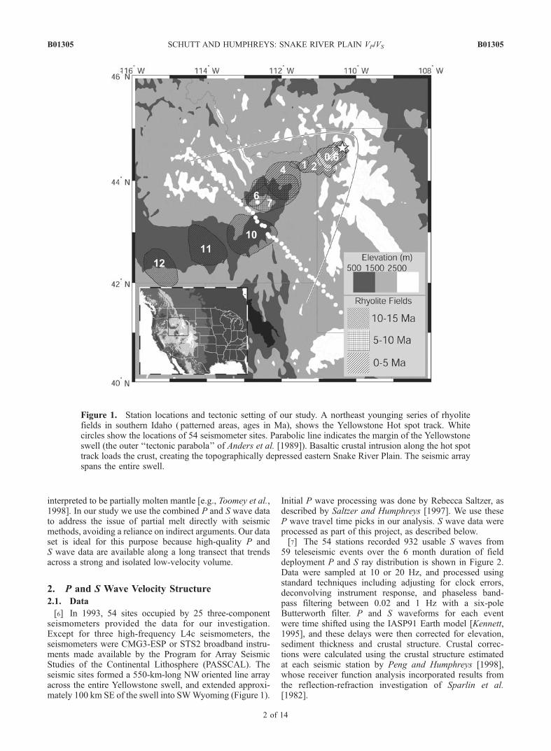
[2] Yellowstone is the most prominent and best knowncontinental hot spot. As it propagated across easternIdaho to its current location in NW Wyoming, it leftbehind a swath of magmatically altered crust, the easternSnake River Plain (SRP), which lies along the axis of aSW broadening wake-like swell. This behavior is consist-ent with mantle melt release at a focused site that isstationary in a hot spot reference frame, and with the hotand buoyant residuum flattening against the base of thelithosphere as it is dragged to the SW by North Americaplate motion.[3] A line array of seismometers crossing the swell and

SRP where the hot spot was about 6–10 m.y. B.P. providedthe teleseismic data that are the basis for several studies,including ours (Figure 1). Seismically inferred crustalstructure beneath this array allows the crustal load on themantle to be estimated [Peng and Humphreys, 1998];

assuming isostasy, the mantle is calculated to be uniformlyvery buoyant across the width of the swell, and approxi-mately of normal continental buoyancy southeast of theswell. Split SKS arrivals recorded by this array indicate thatacross the width of the swell there exists a simple mantleanisotropy aligned nearly in the direction of North Americaplate transport [Schutt et al., 1998]. This stands in contrastto the pattern of anisotropy away from the swell, which ismore complex [Schutt and Humphreys, 2001]. These find-ings are consistent with a mantle plume origin for Yellow-stone.[4] Upper mantle P wave velocity is found to be anom-

alously slow only beneath the SRP [Evans, 1982; Duekerand Humphreys, 1990], whereas mantle beneath the remain-der of the swell is fast compared to average western U.S.upper mantle and rather typical of global average uppermantle [Humphreys and Dueker, 1994]. The zone of low-velocity upper mantle extends to depths of at least 200 km[Saltzer and Humphreys, 1997]. Using seismic velocity andbuoyancy estimates, they interpret the low-velocity mantleto be partially molten.[5] While melt at such great depths has been considered

unreasonable [e.g., McKenzie and Bickle, 1988], imagingbeneath other areas also has revealed low-velocity zones

JOURNAL OF GEOPHYSICAL RESEARCH, VOL. 109, B01305, doi:10.1029/2003JB002442, 2004

1Now at the Department of Geology and Geophysics, University ofWyoming, Laramie, Wyoming, USA.

Copyright 2004 by the American Geophysical Union.0148-0227/04/2003JB002442$09.00

B01305 1 of 14

interpreted to be partially molten mantle [e.g., Toomey et al.,1998]. In our study we use the combined P and S wave datato address the issue of partial melt directly with seismicmethods, avoiding a reliance on indirect arguments. Our dataset is ideal for this purpose because high-quality P andS wave data are available along a long transect that trendsacross a strong and isolated low-velocity volume.

2. P and S Wave Velocity Structure

2.1. Data

[6] In 1993, 54 sites occupied by 25 three-componentseismometers provided the data for our investigation.Except for three high-frequency L4c seismometers, theseismometers were CMG3-ESP or STS2 broadband instru-ments made available by the Program for Array SeismicStudies of the Continental Lithosphere (PASSCAL). Theseismic sites formed a 550-km-long NW oriented line arrayacross the entire Yellowstone swell, and extended approxi-mately 100 km SE of the swell into SWWyoming (Figure 1).

Initial P wave processing was done by Rebecca Saltzer, asdescribed by Saltzer and Humphreys [1997]. We use theseP wave travel time picks in our analysis. S wave data wereprocessed as part of this project, as described below.[7] The 54 stations recorded 932 usable S waves from

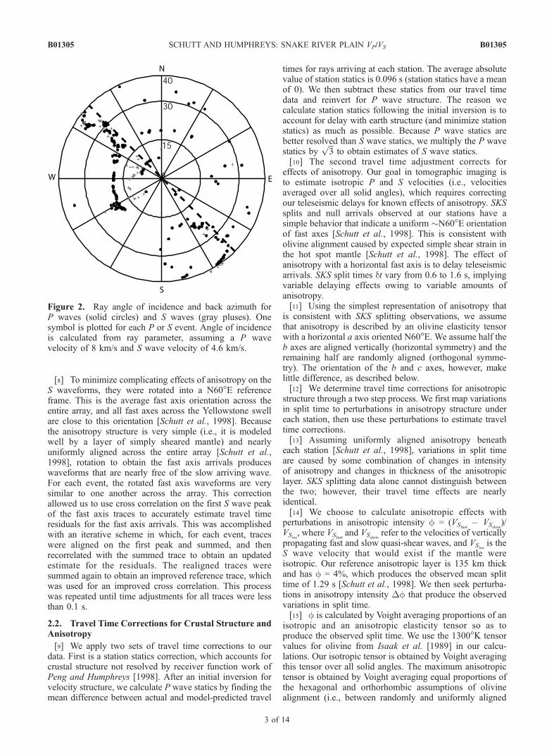
59 teleseismic events over the 6 month duration of fielddeployment P and S ray distribution is shown in Figure 2.Data were sampled at 10 or 20 Hz, and processed usingstandard techniques including adjusting for clock errors,deconvolving instrument response, and phaseless band-pass filtering between 0.02 and 1 Hz with a six-poleButterworth filter. P and S waveforms for each eventwere time shifted using the IASP91 Earth model [Kennett,1995], and these delays were then corrected for elevation,sediment thickness and crustal structure. Crustal correc-tions were calculated using the crustal structure estimatedat each seismic station by Peng and Humphreys [1998],whose receiver function analysis incorporated results fromthe reflection-refraction investigation of Sparlin et al.[1982].

Figure 1. Station locations and tectonic setting of our study. A northeast younging series of rhyolitefields in southern Idaho ( patterned areas, ages in Ma), shows the Yellowstone Hot spot track. Whitecircles show the locations of 54 seismometer sites. Parabolic line indicates the margin of the Yellowstoneswell (the outer ‘‘tectonic parabola’’ of Anders et al. [1989]). Basaltic crustal intrusion along the hot spottrack loads the crust, creating the topographically depressed eastern Snake River Plain. The seismic arrayspans the entire swell.

B01305 SCHUTT AND HUMPHREYS: SNAKE RIVER PLAIN VP/VS

2 of 14

B01305

[8] To minimize complicating effects of anisotropy on theS waveforms, they were rotated into a N60�E referenceframe. This is the average fast axis orientation across theentire array, and all fast axes across the Yellowstone swellare close to this orientation [Schutt et al., 1998]. Becausethe anisotropy structure is very simple (i.e., it is modeledwell by a layer of simply sheared mantle) and nearlyuniformly aligned across the entire array [Schutt et al.,1998], rotation to obtain the fast axis arrivals produceswaveforms that are nearly free of the slow arriving wave.For each event, the rotated fast axis waveforms are verysimilar to one another across the array. This correctionallowed us to use cross correlation on the first S wave peakof the fast axis traces to accurately estimate travel timeresiduals for the fast axis arrivals. This was accomplishedwith an iterative scheme in which, for each event, traceswere aligned on the first peak and summed, and thenrecorrelated with the summed trace to obtain an updatedestimate for the residuals. The realigned traces weresummed again to obtain an improved reference trace, whichwas used for an improved cross correlation. This processwas repeated until time adjustments for all traces were lessthan 0.1 s.

2.2. Travel Time Corrections for Crustal Structure andAnisotropy

[9] We apply two sets of travel time corrections to ourdata. First is a station statics correction, which accounts forcrustal structure not resolved by receiver function work ofPeng and Humphreys [1998]. After an initial inversion forvelocity structure, we calculate P wave statics by finding themean difference between actual and model-predicted travel

times for rays arriving at each station. The average absolutevalue of station statics is 0.096 s (station statics have a meanof 0). We then subtract these statics from our travel timedata and reinvert for P wave structure. The reason wecalculate station statics following the initial inversion is toaccount for delay with earth structure (and minimize stationstatics) as much as possible. Because P wave statics arebetter resolved than S wave statics, we multiply the P wavestatics by

ffiffiffi3

pto obtain estimates of S wave statics.

[10] The second travel time adjustment corrects foreffects of anisotropy. Our goal in tomographic imaging isto estimate isotropic P and S velocities (i.e., velocitiesaveraged over all solid angles), which requires correctingour teleseismic delays for known effects of anisotropy. SKSsplits and null arrivals observed at our stations have asimple behavior that indicate a uniform �N60�E orientationof fast axes [Schutt et al., 1998]. This is consistent witholivine alignment caused by expected simple shear strain inthe hot spot mantle [Schutt et al., 1998]. The effect ofanisotropy with a horizontal fast axis is to delay teleseismicarrivals. SKS split times dt vary from 0.6 to 1.6 s, implyingvariable delaying effects owing to variable amounts ofanisotropy.[11] Using the simplest representation of anisotropy that

is consistent with SKS splitting observations, we assumethat anisotropy is described by an olivine elasticity tensorwith a horizontal a axis oriented N60�E. We assume half theb axes are aligned vertically (horizontal symmetry) and theremaining half are randomly aligned (orthogonal symme-try). The orientation of the b and c axes, however, makelittle difference, as described below.[12] We determine travel time corrections for anisotropic

structure through a two step process. We first map variationsin split time to perturbations in anisotropy structure undereach station, then use these perturbations to estimate traveltime corrections.[13] Assuming uniformly aligned anisotropy beneath

each station [Schutt et al., 1998], variations in split timeare caused by some combination of changes in intensityof anisotropy and changes in thickness of the anisotropiclayer. SKS splitting data alone cannot distinguish betweenthe two; however, their travel time effects are nearlyidentical.[14] We choose to calculate anisotropic effects with

perturbations in anisotropic intensity f = (VSfast� VSslow

)/VSiso

, where VSfastand VSslow

refer to the velocities of verticallypropagating fast and slow quasi-shear waves, and VSiso

is theS wave velocity that would exist if the mantle wereisotropic. Our reference anisotropic layer is 135 km thickand has f = 4%, which produces the observed mean splittime of 1.29 s [Schutt et al., 1998]. We then seek perturba-tions in anisotropy intensity �f that produce the observedvariations in split time.[15] f is calculated by Voight averaging proportions of an

isotropic and an anisotropic elasticity tensor so as toproduce the observed split time. We use the 1300�K tensorvalues for olivine from Isaak et al. [1989] in our calcu-lations. Our isotropic tensor is obtained by Voight averagingthis tensor over all solid angles. The maximum anisotropictensor is obtained by Voight averaging equal proportions ofthe hexagonal and orthorhombic assumptions of olivinealignment (i.e., between randomly and uniformly aligned

Figure 2. Ray angle of incidence and back azimuth forP waves (solid circles) and S waves (gray pluses). Onesymbol is plotted for each P or S event. Angle of incidenceis calculated from ray parameter, assuming a P wavevelocity of 8 km/s and S wave velocity of 4.6 km/s.


3 of 14

B01305

b axes), though in our application, it makes little differencewhether we use a hexagonal or orthorhombic tensor.[16] With these assumptions,

�f ¼ 0:029ð�dtÞ ð1Þ

where �dt is the deviation in split time from 1.29 s. Verticalwave speed then varies with f as

VP ¼ VPiso� 7:24ð�fÞ ð2aÞ

VSfast ¼ VSiso � 1:50ð�fÞ ð2bÞ

VSslow ¼ VSiso � 5:97ð�fÞ: ð2cÞ

[17] The coefficients in this relation do not changeappreciably for rays with back azimuths along the strike

of the array propagating up to 30� off vertical. The fewsignificantly off vertical rays that come in perpendicular tothe array strike would see higher velocities, but there are toofew of these rays to affect the resulting velocity image.Equations (1) and (2) combine to yield

�tP ¼ 0:50ð�dtÞ ð3aÞ

�tS ¼ 0:31ð�dtÞ: ð3bÞ

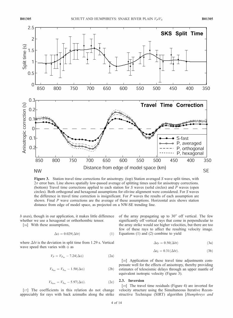
[18] Application of these travel time adjustments com-pensate well for the effects of anisotropy, thereby providingestimates of teleseismic delays through an upper mantle ofequivalent isotropic velocity (Figure 3).

2.3. Inversion

[19] The travel time residuals (Figure 4) are inverted forvelocity structure using the Simultaneous Iterative Recon-structive Technique (SIRT) algorithm [Humphreys and

Figure 3. Station travel time corrections for anisotropy. (top) Station averaged S wave split times, with2s error bars. Line shows spatially low-passed average of splitting times used for anisotropy corrections.(bottom) Travel time corrections applied to each station for S waves (solid circles) and P waves (opencircles). Both orthogonal and hexagonal assumptions for olivine alignment were considered. For S wavesthe difference in travel time correction is insignificant. For P waves the results of each assumption areshown. Final P wave corrections are the average of these assumptions. Horizontal axis shows stationdistance from edge of model space, as projected on a NW-SE trending line.


4 of 14

B01305

Clayton, 1988; Nolet, 1993]. Ray paths were calculatedusing Snell’s law to guide rays through Grand’s [1994]tectonic North America radial velocity structure. Saltzer andHumphreys [1997] show that with SRP data, choice ofreference radial velocity structure and use of 3-D ray tracingmake only imperceptible differences in inversion results.They also show that for the upper mantle structure beneaththis array, differences between inversions produced by theSIRT and LSQR algorithms are inconsequential [Paige andSaunders, 1982].[20] The seismic array is a line oriented toward the back

azimuths of most global seismicity, and it trends perpendic-ular to the hot spot track and known upper mantle structure(Figure 5) [Evans, 1982; Humphreys and Dueker, 1994].This deployment geometry is designed to provide a high-resolution 2-D cross section across the Yellowstone swellperpendicular to the SRP. The tomographic model (Figure 5)is aligned with the seismic array. It extends 1200 km in thedirection of the array (i.e., N45�W), is 200 km wide in thecross-array direction, is centered on the SRP, and extends toa depth of 450 km. The model consists of blocks 10 kmdeep and 10 km wide in the direction of the array. Blocksextend 200 km to the SW of the array. This model geometry

provides a 2-D inversion for structure SW of the array,through which most of the rays travel. Structure to the NEof the array is similar, but resolution is poorer, and weconfine our study to the SW volume. Ray coverage isshown in Figure 6. Figure 7 shows results of straightforwardinversion of the anisotropy-corrected S wave travel timeresiduals, using the Simultaneous Iterative ReconstructiveTechnique (SIRT) [Gilbert, 1972; Humphreys and Clayton,1988]. Results are similar if data are limited to nearlyvertical rays and rays with back azimuths along the strikeof the array.[21] A prominent low-velocity zone is imaged beneath

the center of the array extending from the surface to about200 km in depth. The NW dip of the low-velocity zone isthought to be authentic because inversions of syntheticrectangular-shaped vertical structures do not produce dip-ping structures. With our teleseismic rays, which all arrivewithin 40� of vertical, the horizontal position of the low-velocity body is well resolved (Figures 8a and 8b). Appli-cation of anisotropy corrections have a small but noticableeffect on imaged structure. They do not change overallcharacter of inversion or any of the findings discussedbelow.

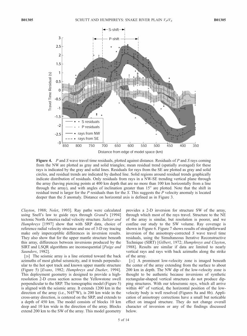
Figure 4. P and S wave travel time residuals, plotted against distance. Residuals of P and S rays comingfrom the NW are plotted as gray and solid triangles; mean residual trend (spatially averaged) for theserays is indicated by the gray and solid lines. Residuals for rays from the SE are plotted as gray and solidcircles, and residual trends are indicated by dashed line. Solid regions around residual trends graphicallyindicate distribution of residuals. Only residuals from rays in a NW-SE trending vertical plane throughthe array (having piercing points at 400 km depth that are no more than 100 km horizontally from a linethrough the array), and with angles of inclination greater than 15� are plotted. Note that the shift inresidual trend is larger for the P residuals than for the S. This suggests the P velocity anomaly is locateddeeper than the S anomaly. Distance on horizontal axis is defined as in Figure 3.


5 of 14

B01305

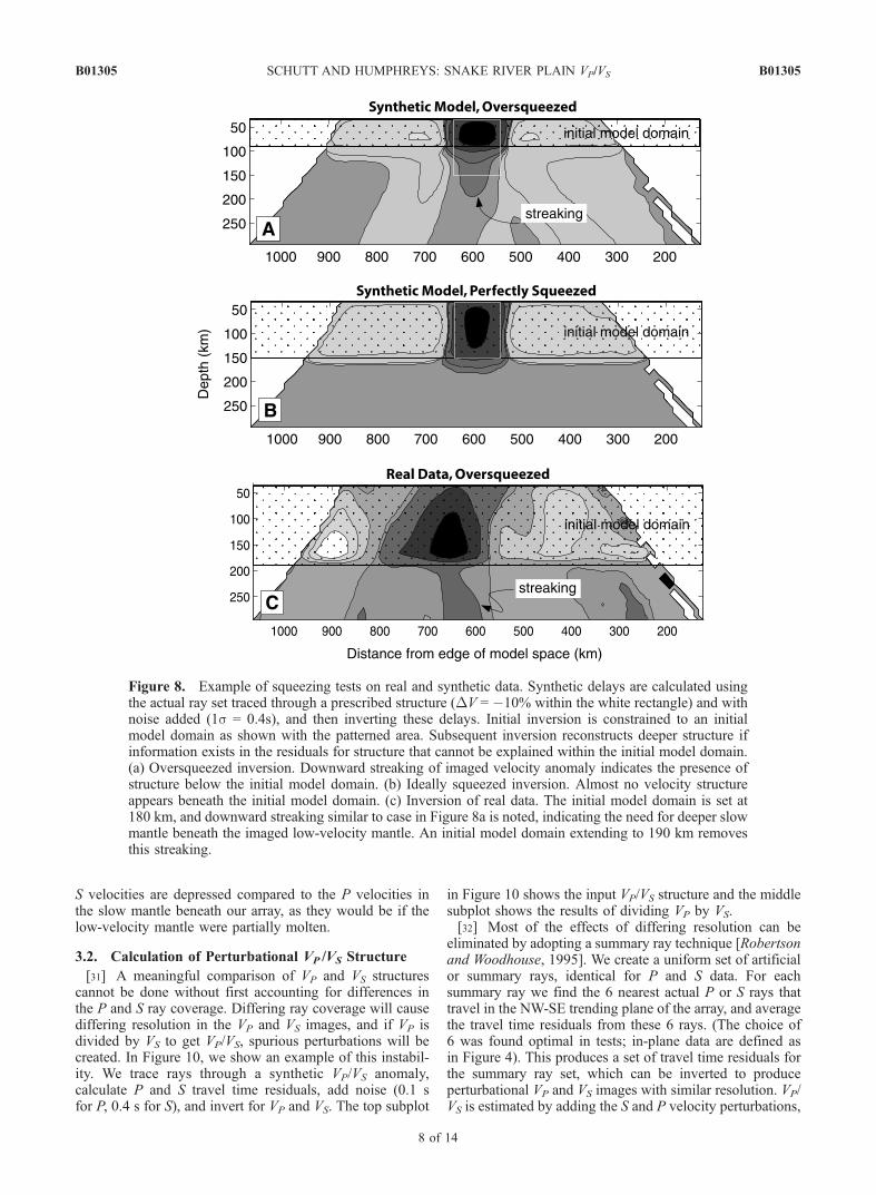
[22] In contrast to excellent horizontal resolution, verti-cal resolution of structure is relatively poor. This is a resultof vertical ‘‘streaking,’’ which is well understood to be theprimary resolution problem in upper mantle teleseismictomography. Streaks are artifacts extending away fromactual structures in directions commonly taken by rays(Figures 7, 8a, and 8c), often with increases in amplitudewhere the streaks meet the boundaries of the model. Moreprecisely, streaks occur where a lack of crossing raysresults in a model that is locally underdetermined, and abroadly distributed feature is produced by the implicittendency of inversion to create a model of minimumenergy (in addition to any other constraints beingimposed). Keller et al. [2000] and Wolfe et al. [2002]discuss this resolution problem with respect to imagingbeneath Iceland. The low-velocity streaks that trend awayfrom the prominent low-velocity structure beneath the SRP(at �30� from vertical) are typical of these artifacts. Thisis confirmed by testing resolution of structures confined inthe uppermost mantle beneath the SRP, which producesimilar streaks upon inversion.[23] To assess our ability to resolve the depth limits of the

SRP low-velocity zone, we make use of vertical ‘‘squeez-ing’’ experiments that test the need for structure outside ofspecified depth limits [Saltzer and Humphreys, 1997]. Theprinciple is to hypothesis test for permissibility of a depthlimit constraint by testing if any information in the data issignificantly in contradiction with the constraint. In our

tests, we invert data in a normal fashion except that structureis allowed only within a specified depth range (e.g., onlybetween 90 and 150 km). This constraint is then relaxed andstructure is allowed to be reconstructed throughout themodel. The initial depth-constrained inversion results inthe least squares best model within the prescribed depthrange, which we term the ‘‘initial model domain’’, and ityields travel time residuals with respect to this model. Theseresiduals (which cannot be explained by the depth-con-strained model) are themselves inverted for structure in thefull model space and added to the original model, just as isnormal for an additional SIRT inversion. If all residualswere zero, we produce no new structure; if the residuals arerandom values, then we would produce essentially no newstructure. Only if a better model exists (in a least squaressense) is the updated structure different from the initialstructure, and this is recognized by the inclusion of signif-icant structure outside the initial model domain. An exampleof a squeezing test on synthetic data is shown in Figures 8aand 8b.[24] To test the need for near surface and deep structure,

we run two series of squeezing tests. In each series of tests,we invert for structure within the initial model domain using5 SIRT iterations, then extend the area of allowed structureinto the whole model space for 15 more iterations. In thesetests, the initial model domain is above 300 km, which is thegreatest depth for which there are crossing rays, and hencerelatively good resolution.[25] The first series of inversions test the necessity of near

surface structure. We test a range of depths for the top of theinitial model domain ranging from 30 to 210 km in 10 kmintervals, with the bottom held at 300 km, and look forcoherent near-surface structure to develop after we relax thesqueezing constraint. When the top of the initial modeldomain is located below about 80 km, both the P andS inversions develop a coherent low-velocity region abovethis bound. Thus a model that extends between 80 and300 km explains the data about as well as possible, but amodel with a top deeper than 80 km in depth begins toviolate information contained in the data.

Figure 5. Modeled volume of tomographic inversion.Modeled volume is 800 km long, 200 km wide (outlineshown with heavy lines), and 450 km deep. Model blocksare indicated with the thin tick marks. In this study weconsider structure to the SW side of the array. Individualmodel blocks are 10 km wide (NW-SE), 15 km deep, andextend 200 km in the NE-SW direction. Solid circles are raypiercing points at 300 km depth. Open circles are stationlocations. Origin used for distance measurements markedwith a hexagon.

Figure 6. Hit count in model blocks, as represented bytotal ray length through each block (in km). Region of goodcrossing ray coverage extends to about 300 km beneath thearray center.


6 of 14

B01305

[26] The second set of squeezing inversions tests for deepstructure. We test depths for the bottom of the initial modeldomain ranging from 100 to 300 km at 10 km intervals,while keeping the top of the domain at 30 km. A low-velocity region appears beneath the bottom of the initialmodel domain when it is located at a depth above 190 km,indicating that velocity structure extends to at least 190 km(Figure 8c), and is not required beneath this depth.[27] These squeezing tests indicate that velocity structure

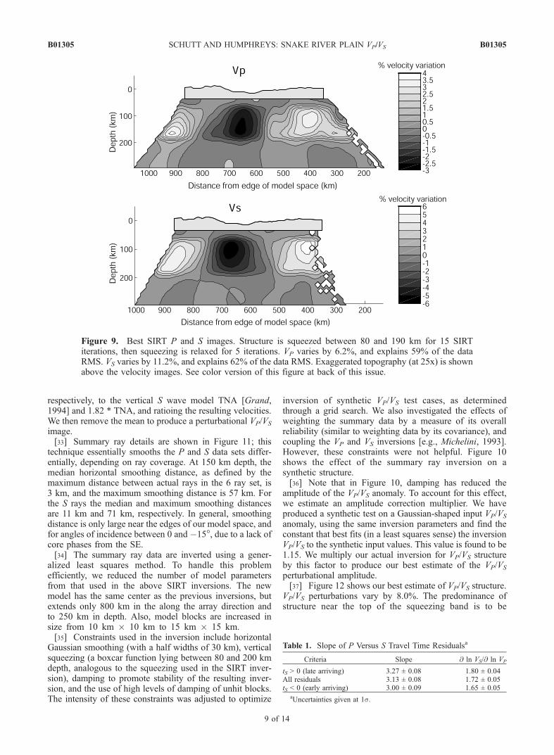
necessarily exists between depths of 80 and 190 km. Thefact that no structure is required outside of these bounds,combined with the observation that tests on simple syntheticstructures outside these bounds can be at least partiallyresolved, suggests that actual earth structure is largelyconfined to within these limits.[28] Figure 9 shows our best estimate of perturbational P

and S velocity structure beneath the array, based on aninitial model domain extending from 80 to 190 km.P velocity varies by 6.2% in this image, and S velocityvaries by 11.2%. Note that our squeezing removes most ofthe dipping trend of the P low-velocity zone in Figure 7.This image VP structure is very similar to that obtained bySaltzer and Humphreys [1997], indicating that the effects ofthe anisotropy corrections are relatively minor. The VS

structure differs slightly from the VP in that the area oflow velocity is shallower. We further examine differencesbetween VP and VS below.

3. VP///VS Structure

[29] Because P and S wave velocities have differentsensitivities to partial melt, temperature, and composition,a combination of VP and VS provides more insight intomantle physical state than either VP or VS alone. In partic-ular, VS is more sensitive to the presence of melt than is VP

(while being similarly sensitive to composition and temper-ature), hence, VP/VS can be used to distinguish regions ofpartial melt. In this section, we first compare the P andS travel time residuals to demonstrate that systematic differ-ences exist between these data sets. We then invert thesedata for perturbational VP/VS structure. Unlike the VP and VS

tomography inversions, where spatial resolution is maxi-mized, the VP/VS inversion is optimized for correct ampli-tudes. The resulting tomogram will then be used to estimatethe physical state of the mantle.

3.1. Comparison of P and S Data

[30] Figure 4 shows P and S travel time residuals forevents of opposing back azimuth. The shift in the S waveresidual pattern is less than that for P waves, implying thatthe centroid of the S wave low-velocity zone is shallowerthan that of the P wave low-velocity zone. Also, the lateraltransitions in S delays are greater, implying a greaterhorizontal velocity gradient near the boundaries of the VS

low-velocity anomaly. To further consider these differences,we compare P and S wave travel time residuals for rays thatshare common paths. The ratio of the S wave residuals dts tothe P wave residuals dtp is related to the material seismicvelocities VP and VS by [Hales and Herrin, 1972]

dtSdtP

� @ lnVS

@ lnVP

VP

VS

� �: ð4Þ

By applying the least squares method [York, 1966] to fitlines to the data (using a S residual picking error of 0.4 s, aP picking error of 0.1 s, and assuming VP/VS to be 1.82, theIASP91 [Kennett, 1995] value at 180 km depth), we find @ln VS/@ ln VP to be 8% greater for the late arriving rays thanthe early arriving rays (Table 1). This corresponds toPoisson’s ratio increasing from 0.25 to 0.28. Thus the

Figure 7. Initial SIRT inversion of S wave data. Contour interval is 1%. Anisotropic corrections areshown at the top. These corrections are small and uncorrelated with the imaged isotropic structure. Sincethe S wave rays are nearly vertically incident, vertical resolution is limited, causing streaking of velocityfeatures along the paths most commonly taken by rays. The structure labeled streaking are typical of thisbehavior, and in all likelihood are artifacts.


7 of 14

B01305

S velocities are depressed compared to the P velocities inthe slow mantle beneath our array, as they would be if thelow-velocity mantle were partially molten.

3.2. Calculation of Perturbational VP //VS Structure

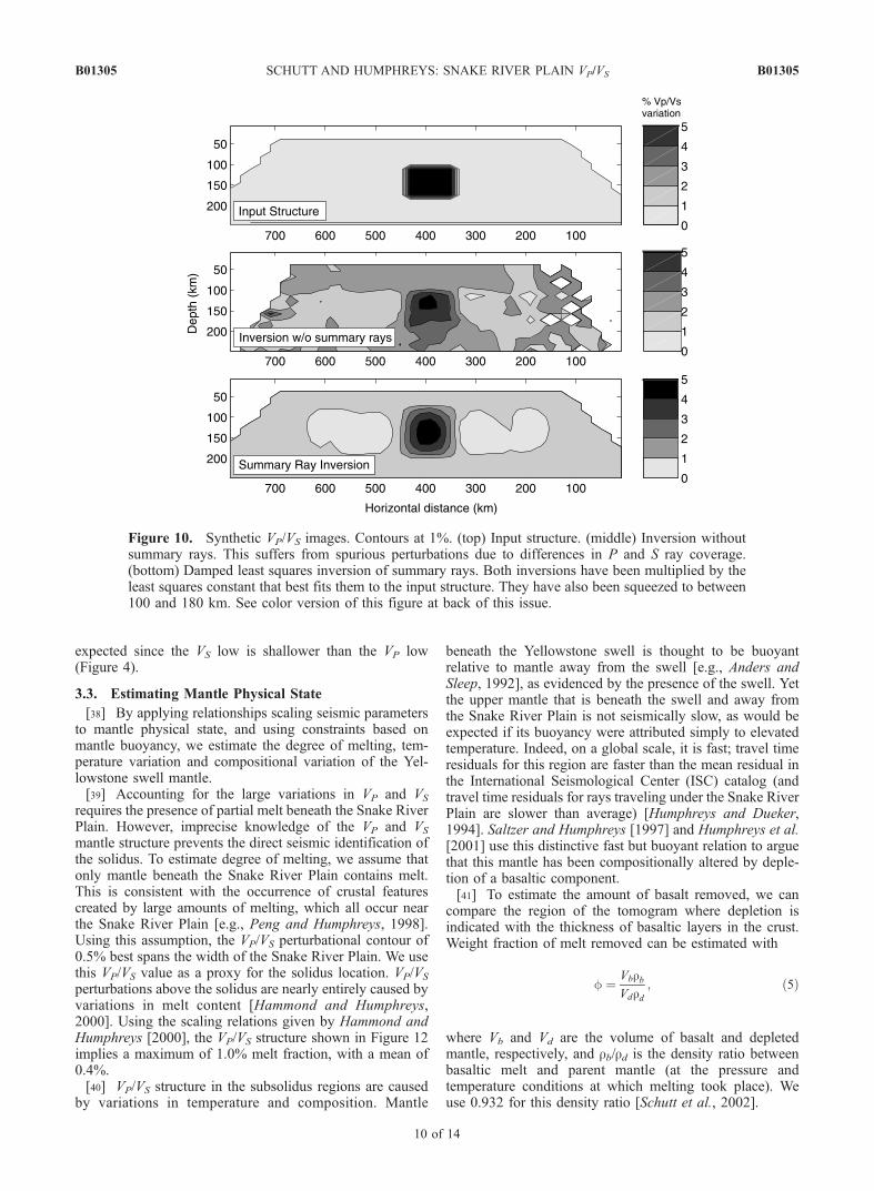
[31] A meaningful comparison of VP and VS structurescannot be done without first accounting for differences inthe P and S ray coverage. Differing ray coverage will causediffering resolution in the VP and VS images, and if VP isdivided by VS to get VP/VS, spurious perturbations will becreated. In Figure 10, we show an example of this instabil-ity. We trace rays through a synthetic VP/VS anomaly,calculate P and S travel time residuals, add noise (0.1 sfor P, 0.4 s for S), and invert for VP and VS. The top subplot

in Figure 10 shows the input VP/VS structure and the middlesubplot shows the results of dividing VP by VS.[32] Most of the effects of differing resolution can be

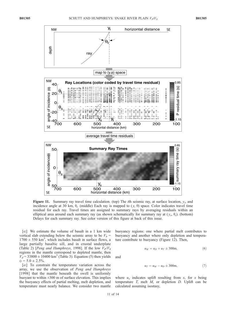
eliminated by adopting a summary ray technique [Robertsonand Woodhouse, 1995]. We create a uniform set of artificialor summary rays, identical for P and S data. For eachsummary ray we find the 6 nearest actual P or S rays thattravel in the NW-SE trending plane of the array, and averagethe travel time residuals from these 6 rays. (The choice of6 was found optimal in tests; in-plane data are defined asin Figure 4). This produces a set of travel time residuals forthe summary ray set, which can be inverted to produceperturbational VP and VS images with similar resolution. VP/VS is estimated by adding the S and P velocity perturbations,

Figure 8. Example of squeezing tests on real and synthetic data. Synthetic delays are calculated usingthe actual ray set traced through a prescribed structure (�V = �10% within the white rectangle) and withnoise added (1s = 0.4s), and then inverting these delays. Initial inversion is constrained to an initialmodel domain as shown with the patterned area. Subsequent inversion reconstructs deeper structure ifinformation exists in the residuals for structure that cannot be explained within the initial model domain.(a) Oversqueezed inversion. Downward streaking of imaged velocity anomaly indicates the presence ofstructure below the initial model domain. (b) Ideally squeezed inversion. Almost no velocity structureappears beneath the initial model domain. (c) Inversion of real data. The initial model domain is set at180 km, and downward streaking similar to case in Figure 8a is noted, indicating the need for deeper slowmantle beneath the imaged low-velocity mantle. An initial model domain extending to 190 km removesthis streaking.


8 of 14

B01305

respectively, to the vertical S wave model TNA [Grand,1994] and 1.82 * TNA, and ratioing the resulting velocities.We then remove the mean to produce a perturbational VP/VS

image.[33] Summary ray details are shown in Figure 11; this

technique essentially smooths the P and S data sets differ-entially, depending on ray coverage. At 150 km depth, themedian horizontal smoothing distance, as defined by themaximum distance between actual rays in the 6 ray set, is3 km, and the maximum smoothing distance is 57 km. Forthe S rays the median and maximum smoothing distancesare 11 km and 71 km, respectively. In general, smoothingdistance is only large near the edges of our model space, andfor angles of incidence between 0 and �15�, due to a lack ofcore phases from the SE.[34] The summary ray data are inverted using a gener-

alized least squares method. To handle this problemefficiently, we reduced the number of model parametersfrom that used in the above SIRT inversions. The newmodel has the same center as the previous inversions, butextends only 800 km in the along the array direction andto 250 km in depth. Also, model blocks are increased insize from 10 km � 10 km to 15 km � 15 km.[35] Constraints used in the inversion include horizontal

Gaussian smoothing (with a half widths of 30 km), verticalsqueezing (a boxcar function lying between 80 and 200 kmdepth, analogous to the squeezing used in the SIRT inver-sion), damping to promote stability of the resulting inver-sion, and the use of high levels of damping of unhit blocks.The intensity of these constraints was adjusted to optimize

inversion of synthetic VP/VS test cases, as determinedthrough a grid search. We also investigated the effects ofweighting the summary data by a measure of its overallreliability (similar to weighting data by its covariance), andcoupling the VP and VS inversions [e.g., Michelini, 1993].However, these constraints were not helpful. Figure 10shows the effect of the summary ray inversion on asynthetic structure.[36] Note that in Figure 10, damping has reduced the

amplitude of the VP/VS anomaly. To account for this effect,we estimate an amplitude correction multiplier. We haveproduced a synthetic test on a Gaussian-shaped input VP/VS

anomaly, using the same inversion parameters and find theconstant that best fits (in a least squares sense) the inversionVP/VS to the synthetic input values. This value is found to be1.15. We multiply our actual inversion for VP/VS structureby this factor to produce our best estimate of the VP/VS

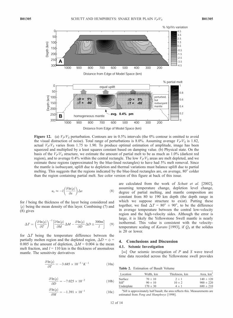
perturbational amplitude.[37] Figure 12 shows our best estimate of VP/VS structure.

VP/VS perturbations vary by 8.0%. The predominance ofstructure near the top of the squeezing band is to be

Figure 9. Best SIRT P and S images. Structure is squeezed between 80 and 190 km for 15 SIRTiterations, then squeezing is relaxed for 5 iterations. VP varies by 6.2%, and explains 59% of the dataRMS. VS varies by 11.2%, and explains 62% of the data RMS. Exaggerated topography (at 25x) is shownabove the velocity images. See color version of this figure at back of this issue.

Table 1. Slope of P Versus S Travel Time Residualsa

Criteria Slope @ ln VS/@ ln VP

tS > 0 (late arriving) 3.27 ± 0.08 1.80 ± 0.04All residuals 3.13 ± 0.08 1.72 ± 0.05tS < 0 (early arriving) 3.00 ± 0.09 1.65 ± 0.05

aUncertainties given at 1s.


9 of 14

B01305

expected since the VS low is shallower than the VP low(Figure 4).

3.3. Estimating Mantle Physical State

[38] By applying relationships scaling seismic parametersto mantle physical state, and using constraints based onmantle buoyancy, we estimate the degree of melting, tem-perature variation and compositional variation of the Yel-lowstone swell mantle.[39] Accounting for the large variations in VP and VS

requires the presence of partial melt beneath the Snake RiverPlain. However, imprecise knowledge of the VP and VS

mantle structure prevents the direct seismic identification ofthe solidus. To estimate degree of melting, we assume thatonly mantle beneath the Snake River Plain contains melt.This is consistent with the occurrence of crustal featurescreated by large amounts of melting, which all occur nearthe Snake River Plain [e.g., Peng and Humphreys, 1998].Using this assumption, the VP/VS perturbational contour of0.5% best spans the width of the Snake River Plain. We usethis VP/VS value as a proxy for the solidus location. VP/VS

perturbations above the solidus are nearly entirely caused byvariations in melt content [Hammond and Humphreys,2000]. Using the scaling relations given by Hammond andHumphreys [2000], the VP/VS structure shown in Figure 12implies a maximum of 1.0% melt fraction, with a mean of0.4%.[40] VP/VS structure in the subsolidus regions are caused

by variations in temperature and composition. Mantle

beneath the Yellowstone swell is thought to be buoyantrelative to mantle away from the swell [e.g., Anders andSleep, 1992], as evidenced by the presence of the swell. Yetthe upper mantle that is beneath the swell and away fromthe Snake River Plain is not seismically slow, as would beexpected if its buoyancy were attributed simply to elevatedtemperature. Indeed, on a global scale, it is fast; travel timeresiduals for this region are faster than the mean residual inthe International Seismological Center (ISC) catalog (andtravel time residuals for rays traveling under the Snake RiverPlain are slower than average) [Humphreys and Dueker,1994]. Saltzer and Humphreys [1997] and Humphreys et al.[2001] use this distinctive fast but buoyant relation to arguethat this mantle has been compositionally altered by deple-tion of a basaltic component.[41] To estimate the amount of basalt removed, we can

compare the region of the tomogram where depletion isindicated with the thickness of basaltic layers in the crust.Weight fraction of melt removed can be estimated with

f ¼ VbrbVdrd

; ð5Þ

where Vb and Vd are the volume of basalt and depletedmantle, respectively, and rb/rd is the density ratio betweenbasaltic melt and parent mantle (at the pressure andtemperature conditions at which melting took place). Weuse 0.932 for this density ratio [Schutt et al., 2002].

Figure 10. Synthetic VP/VS images. Contours at 1%. (top) Input structure. (middle) Inversion withoutsummary rays. This suffers from spurious perturbations due to differences in P and S ray coverage.(bottom) Damped least squares inversion of summary rays. Both inversions have been multiplied by theleast squares constant that best fits them to the input structure. They have also been squeezed to between100 and 180 km. See color version of this figure at back of this issue.


10 of 14

B01305

[42] We estimate the volume of basalt in a 1 km widevertical slab extending below the seismic array to be Vb =1700 ± 550 km3, which includes basalt in surface flows, alarge partially basaltic sill, and in crustal underplate(Table 2) [Peng and Humphreys, 1998]. If the low VP/VS

regions in the mantle correspond to depleted mantle, thenVd = 33800 ± 10400 km3 (Table 3). Equation (5) then yieldsf = 5.0 ± 2.5%.[43] To constrain the temperature variation across the

array, we use the observation of Peng and Humphreys[1998] that the mantle beneath the swell is uniformlybuoyant to within ±300 m of surface elevation. This impliesthe buoyancy effects of partial melting, melt depletion, andtemperature must nearly balance. We consider two mantle

buoyancy regions: one where partial melt contributes tobuoyancy and another where only depletion and tempera-ture contribute to buoyancy (Figure 12). Then,

uM ¼ uD þ uT 300m; ð6Þ

and

uT ¼ uM � uD 300m; ð7Þ

where ux indicates uplift resulting from x, for x beingtemperature T, melt M, or depletion D. Uplift can becalculated assuming isostasy,

Figure 11. Summary ray travel time calculation. (top) The ith seismic ray, at surface location, yi, andincidence angle at 30 km, qi. (middle) Each ray is mapped to ( y, q) space. Color indicates travel timeresidual for each ray. Travel times are assigned to summary rays by averaging residuals within anelliptical area around each summary ray (as shown schematically for summary ray at ( ys, qs). (bottom)Delays for each summary ray. See color version of this figure at back of this issue.


11 of 14

B01305

ux � �l@ lnhri@x

� ��x ð8Þ

for l being the thickness of the layer being considered andhri being the mean density of this layer. Combining (7) and(8) gives

�T ¼ @ lnhri@T

� ��1 @ lnhri@M

�M � @ lnhri@D

�D 300m

l

� �ð9Þ

for �T being the temperature difference between thepartially molten region and the depleted region, �D = f =0.005 is the amount of depletion, �M = 0.004 is the meanmelt fraction, and l = 110 km is the thickness of anomalousmantle. The sensitivity derivatives

@ lnhri@T

¼ �3:685� 10�5 K�1 ð10aÞ

@ lnhri@D

¼ �7:025� 10�2 ð10bÞ

@ lnhri@M

¼ �1:391� 10�1 ð10cÞ

are calculated from the work of Schutt et al. [2002],assuming temperature change, depletion level change,degree of partial melting, and mantle composition areconstant from 80 to 190 km depth (the depth range inwhich we suppose structure to exist). Putting thesetogether, we find �T = 80� ± 90�, to be the differencein average temperature between the central low-velocityregion and the high-velocity sides. Although the error islarge, it is likely the Yellowstone Swell mantle is nearlyisothermal. This value is consistent with the velocity-temperature scaling of Karato [1993], if QS at the solidusis 20 or lower.

4. Conclusions and Discussion

4.1. Seismic Investigation

[44] Our seismic investigation of P and S wave traveltime data recorded across the Yellowstone swell provides

Figure 12. (a) VP/VS perturbation. Contours are in 0.5% intervals (the 0% contour is omitted to avoidthe visual distraction of noise). Total range of perturbations is 8.0%. Assuming average VP/VS is 1.82,actual VP/VS varies from 1.75 to 1.90. To produce optimal estimation of amplitude, image has beensqueezed and multiplied by a least squares constant based on damping value. (b) Physical state. On thebasis of the VP/VS structure, we estimate the amount of partial melt to be as much as 1.0% (darkest redregion), and to average 0.4% within the central rectangle. The low VP/VS areas are melt depleted, and weestimate these regions (approximated by the blue-lined rectangles) to have had 5% melt removal. Sincethe mantle is isobuoyant, uplift due to depletion and thermal variations must balance uplift due to partialmelting. This suggests that the regions indicated by the blue-lined rectangles are, on average, 80� colderthan the region containing partial melt. See color version of this figure at back of this issue.

Table 2. Estimation of Basalt Volume

Location Width, km Thickness, km Area, km2

Surface 70 ± 10 2 ± 1 140 ± 120Silla 90 ± 10 10 ± 2 900 ± 220Underplate 170 ± 30 4 ± 1 680 ± 210

aSill is approximately half basalt; the area reflects this. Measurements areestimated from Peng and Humphreys [1998].


12 of 14

B01305

some of the most resolved upper mantle tomographicimages available. This results from having a long andhigh-density line array aligned with most the Earth’s seis-micity and trending perpendicular to the major structures inthe region. We also benefit from (1) the simple and well-resolved anisotropy structure that exists beneath our array[Schutt et al., 1998], which allows us to estimate well andcorrect for the effects of anisotropy on P and S travel times,and (2) the well-resolved crustal corrections on travel time,which result from receiver function analysis constrained byactive source reflection and refraction investigations [Pengand Humphreys, 1998].[45] Even with these advantages, the seismic data by

themselves are insufficient to constrain the depth distribu-tion of structure very well. This problem is intrinsic to thedata; structures of various depth distributions account forthe data equally well. Good control on the depth distributionof structure is provided through the use of squeezing testscombined with plausibility arguments. We find that struc-ture is required to depths of at least 180 km, and there is noneed for structure below 190 km. When structure is imagedbelow 190 km, it has the form expected for streaks related tothe structure imaged above 190 km. These results, com-bined with the geodynamic expectation that temperature andpartial melt variations are minor below 190 km, argue thatno significant structure exists beneath this depth. Similarly,there is no need for mantle structure above 80 km. Becausethe crustal structure (i.e., structure above �40 km) is wellknown from other investigations, and synthetic tests suggestthat we can resolve major structures in the uppermostmantle, we conclude that only modest structure can bepresent between 40 and 80 km.[46] Figure 9, which is constructed under the constraint

that structure is preferred to lie between 80 and 190 km, isour preferred tomographic model of VP and VS structure.Imaged VP and VS structure is quite similar in form. Theamplitude of imaged structure is very large, with a strongvelocity depression roughly beneath the SRP and highvelocities beneath the margins of the Yellowstone swell.VS structure resides at shallower levels than correspondingVP structure. This result can be seen directly in the data(Figure 4), where the P delay pattern shifts with change inincidence angle by amounts greater than the S delay pattern.The high-velocity maxima seen in Figure 9 to lie inboard ofthe side model boundaries are thought to represent actualstructure because travel time delays seen in Figure 3 aresmallest for stations inboard of the array edges.[47] The anisotropy structure and the isotropic structure

do not correlate spatially (Figure 7). Anisotropy correctionsto the travel time delays, at 30% and 6% of the respective Pand S travel time delay RMS, are relatively small butsignificant. Correcting for the travel time effects of anisot-ropy does not significantly change the amplitude of theresulting images, although it does make the VP image lookmore like the VS.

[48] @ ln VS/@ ln VP is resolvably greater for delayedarrivals compared to advanced arrivals (Table 1), implyingthe presence of partial melt in the low-velocity areas.Through the use of summary rays we produce perturbationalVP and VS images of comparable resolution, from which aperturbational VP/VS image is made (Figure 12). This imageconfirms the greater depth of P wave structure compared toS wave structure. VP/VS variations are imaged at about 8%beneath the array, with a prominent VP/VS high beneath theSRP at about 80 km depth. A high gradient in VP/VS isimaged near 80–100 km depth, which is thought to be theupper reaches of partially molten mantle. Resolution testsindicate that this gradient is high; however, we haveinsufficient information to resolve if the gradient is as highas we show, or if it is exaggerated by the constraints used ininversion.

4.2. Physical State

[49] We conclude that the upper mantle is nearly uni-formly hot and buoyant beneath the Yellowstone swell, thatthis mantle is significantly hotter and more buoyant thanadjacent mantle, that the volume of partially molten uppermantle lies roughly beneath the SRP, and that the mantlebeneath the remainder of the swell has been depleted inbasalt and volatiles. By assuming the VP/VS perturbationalcontour of 0.5% represents the solidus, we infer that thevolume of low V and high VP/VS result from the presence ofup to about 1.0% basaltic melt, that the entire upper mantleswell is within �80�K of the solidus, and that swell uppermantle averages �200�K warmer than the surroundingmantle. Dividing the estimated volume of basalt segregatedfrom the mantle by the volume of depleted mantle yields 5 ±2.5% weight fraction of basalt depletion from the swellupper mantle.

4.3. Geodynamics

[50] Much of the inferred upper mantle physical statebeneath the Yellowstone swell can be explained by theplume flattening models such as [Anders and Sleep, 1992].However, these models need to be modified to account forthe strong variations in imaged seismic structure [Saltzerand Humphreys, 1997]. The hot, depleted and essentiallysubsolidus swell mantle away from the SRP must haveexperienced recent melt removal which, in all likelihood,constructed the volcanic structures of the SRP crust bysegregating from the mantle below. The flow of mantle upbeneath the SRP and then to beneath the adjoining areaswould represent convection. The only plausible source ofdensity difference to have driven this convection is meltbuoyancy [e.g., Tackley and Stevenson, 1993], which weinfer continued until accumulating depletion buoyancyequaled the melt buoyancy and terminated upwelling. Thesystem now is nearly static, though it continues to slowlyspread through buoyant flattening as described by Andersand Sleep [1992].[51] Whether or not Yellowstone is a plume that ascends

under the influence of its own negative buoyancy is notresolved by our teleseismic studies, which crosses down-stream of the currently active Yellowstone system. A lowermantle source for the hot spot mantle is suggested by the�200�K excess temperature of the swell upper mantle, highHe3/He4 [Hearn et al., 1990] and lower mantle low veloc-

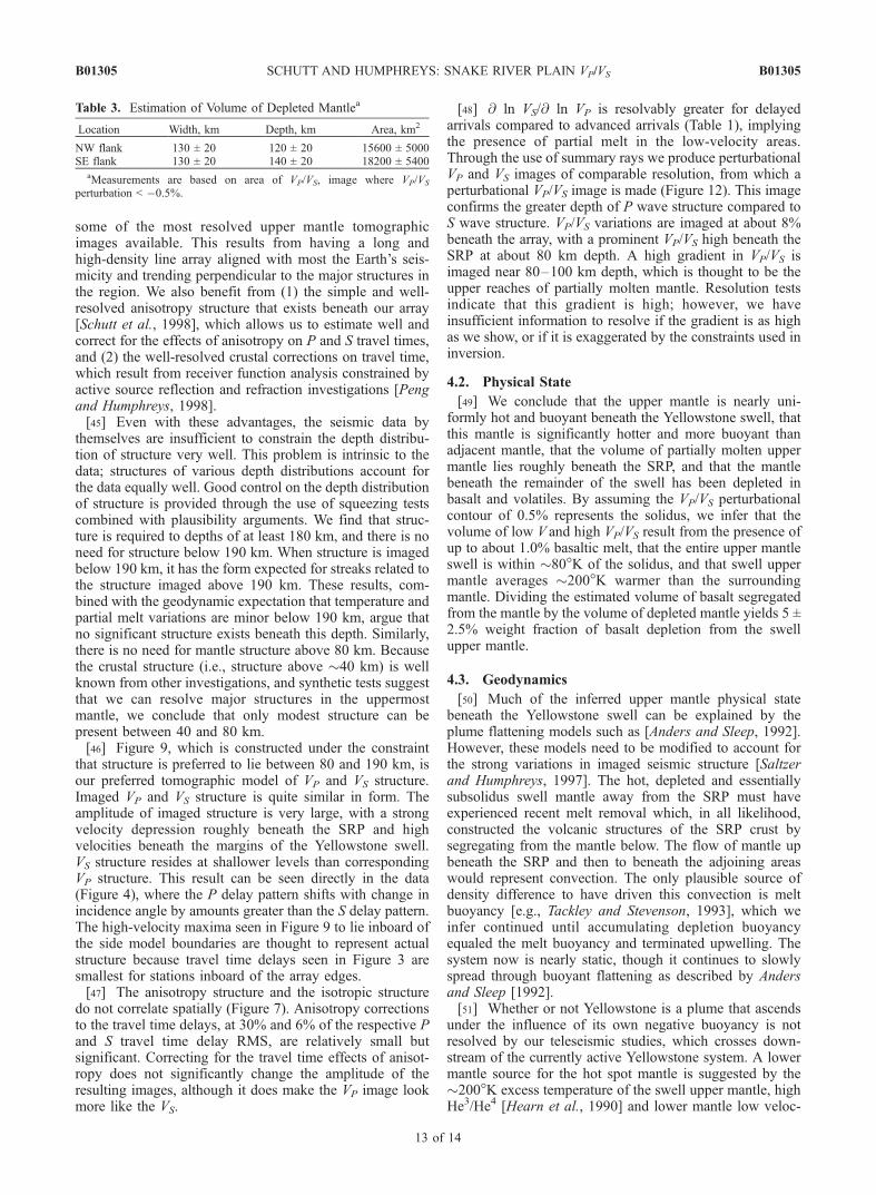
Table 3. Estimation of Volume of Depleted Mantlea

Location Width, km Depth, km Area, km2

NW flank 130 ± 20 120 ± 20 15600 ± 5000SE flank 130 ± 20 140 ± 20 18200 ± 5400

aMeasurements are based on area of VP/VS, image where VP/VS

perturbation < �0.5%.


13 of 14

B01305

ities to at least as deep as 1000 km beneath the generalYellowstone area [Bijwaard et al., 1998]. However, theassociation of Yellowstone with the Newberry hot spot(now in central Oregon) and the tectonic setting that drivesupper mantle divergence [Humphreys et al., 2001] suggestsmuch of the energy driving this system derives itself fromthe upper mantle.

4.4. Summary

[52] To clarify how the Yellowstone hot spot materialevolves as it is dragged by the North America plate, wehave measured seismic velocity and use it to infer mantlephysical state in a cross section across the YellowstoneSwell. We have inverted anisotropically corrected teleseis-mic P and S wave travel times to produce VP and VS images.Inversion tests show that structure is necessary between 80and 190 km in depth, and not required outside this region.The magnitude of the VP and VS variations (6.2% and 11.2%respectively), and a comparison of P and S wave travel timeresiduals, strongly suggest the presence of partial melt underthe Snake River Plain.[53] Using summary rays, we combine the VP and VS

images to calculate VP/VS. From the VP/VS structure, we useseismic and density constraints to estimate the physical stateof the mantle in the Yellowstone Swell. We find about 1.0%melt exists under the Snake River Plain. This melt is flankedby depleted mantle that is within about 80�K of the solidus,and has had about 5% melt removed.[54] Although the velocity and physical state structures

are more accurately known, our view of the geodynamics ofthe Yellowstone system remains as it was set out inHumphreys et al. [2001] and Saltzer and Humphreys[1997].

[55] Acknowledgments. We would like to thank Justin Revenaugh,Karen Fischer, and an anonymous reviewer for helpful comments; also KenDueker for helpful advice and managing the array, This work was supportedby NSF grants EAR-9628474 and EAR-9725598. Data were collectedunder the Program for Array Seismic Studies of the Continental Litho-sphere (PASSCAL) program. D. S. wishes to thank the Carnegie Institutionof Washington for postdoctoral support.

ReferencesAnders, M. H., and N. H. Sleep (1992), Magmatism and extension: Thethermal and mechanical effects of the Yellowstone hotspot, J. Geophys.Res., 97, 15,379–15,393.

Anders, M. H., J. W. Geissman, L. A. Piety, and T. J. Sullivan (1989),Parabolic distribution of circumeastern Snake River Plain seismicity andlatest Quaternary faulting: Migratory and association with the Yellow-stone hot spot, J. Geophys. Res., 94, 1589–1621.

Bijwaard, H., W. Spakman, and E. R. Engdahl (1998), Closing the gapbetween regional and global travel time tomography, J. Geophys. Res.,103, 30,555–30,078.

Dueker, K. G., and E. D. Humphreys (1990), Upper mantle velocity struc-tures of the Great Basin, Geophys. Res. Lett., 17, 1327–1330.

Evans, J. (1982), Compressional wave velocity structure of the upper350 km under the eastern Snake River Plain near Rexburg, Idaho,J. Geophys. Res., 87, 2654–2670.

Gilbert, P. F. C. (1972), Iterative methods for three-dimensional reconstruc-tion of an object from projections, J. Theoret. Biol., 36, 105–117.

Grand, S. P. (1994), Mantle shear structure beneath the Americas andsurrounding oceans, J. Geophys. Res., 99, 11,591–11,621.

Hales, A. L., and E. Herrin (1972), Travel times of seismic waves, in TheNature of the Solid Earth, edited by E. C. Robertson, pp. 172–215,McGraw-Hill, New York.

Hammond, W. C., and E. D. Humphreys (2000), Upper mantle seismicwave velocity: Effects of realistic partial melt geometries, J. Geophys.Res., 105, 10,975–10,986.

Hearn, E. H., B. M. Kennedy, and A. H. Truesdell (1990), Coupled varia-tions in helium isotopes and fluid chemistry; Shoshone Geyser Basin,Yellowstone National Park, Geochim. Cosmochim. Acta, 54, 3103–3113.

Humphreys, E. D., and R. W. Clayton (1988), Adaptation of back projec-tion tomography to seismic travel time problems, J. Geophys. Res., 93,1073–1085.

Humphreys, E. D., and K. G. Dueker (1994), Physical state of the westernU.S. upper mantle, J. Geophys. Res., 99, 9625–9650.

Humphreys, E. D., K. G. Dueker, D. L. Schutt, and R. B. Smith (2001),Beneath Yellowstone: Evaluating plume and nonplume models usingteleseismic images of the upper mantle, GSA Today, 10, 1–7.

Isaak, D. G., O. L. Anderson, and T. Goto (1989), Elasticity of single-crystal Forsterite measured to 1700 K, J. Geophys. Res., 95, 5895–5906.

Karato, S. (1993), Importance of anelasticity in the interpretation of seismictomography, Geophys. Res. Lett., 20, 1623–1626.

Keller, W. R., D. L. Anderson, and R. W. Clayton (2000), Resolution oftomographic models of the mantle beneath Iceland, Geophys. Res. Lett.,27, 3993–3996.

Kennett, B. L. N. (1995), Seismic traveltime tables, in Global EarthPhysics: A Handbook of Physical Constants, AGU Ref. Shelf, vol. 1,edited by T. J. Ahrens, pp. 126–143, AGU, Washington, D. C.

Michelini, A. (1993), Testing the reliability of VP/VS anomalies in travel-time tomography, Geophys. J. Int., 114, 405–410.

McKenzie, D., and M. J. Bickle (1988), The volume and composition ofmelt generated by extension of lithosphere, J. Petrol., 29, 625–679.

Nolet, G. (1993), Solving large linearized tomographic problems, in Seis-mic Tomography, Theory and Practice, edited by H. M. Iyer andK. Hirahara, pp. 248–264, Chapman and Hill, New York.

Paige, C. C., and M. A. Saunders (1982), LSQR: An algorithm for sparselinear equations and sparse least squares, ACM Trans. Math. Software, 8,43–71.

Peng, X., and E. D. Humphreys (1998), Crustal velocity structure across theeastern Snake River Plain and the Yellowstone swell, J. Geophys. Res.,103, 7171–7186.

Robertson, G. S., and J. H. Woodhouse (1995), Evidence for proportion-ality of P and S heterogeneity in the lower mantle, Geophys. J. Int., 123,85–116.

Saltzer, R. L., and E. D. Humphreys (1997), Upper mantle P wave velocitystructure of the eastern Snake River Plain and its relationship to geody-namic models of the region, J. Geophys. Res., 102, 11,829–11,841.

Schutt, D. L., and E. D. Humphreys (2001), Evidence for a deep astheno-sphere from western United States SKS splits, Geology, 29, 291–294.

Schutt, D. L., E. D. Humphreys, and K. Dueker (1998), Anisotropy of theYellowstone hot spot wake, eastern Snake River Plain, Idaho, Pure Appl.Geophys., 151, 443–462.

Schutt, D. L., C. E. Lesher, and J. Pickering-Witter (2002), The effects ofmelt depletion on the density and seismic velocity of garnet and spinellherzolite, Eos Trans., AGU, 83, Spring Meet. Suppl., Abstract M42A-12.

Sparlin, M. A., L. W. Braile, and R. B. Smith (1982), Crustal structure ofthe eastern Snake River Plain from ray trace modeling of seismic refrac-tion data, J. Geophys. Res., 87, 2619–2633.

Tackley, P. J., and D. J. Stevenson (1993), A mechanism for spontaneousself-perpetuating volcanism on the terrestrial planets, in Flow and Creepin the Solar System: Observations, Modeling, and Theory, NATO ASI Ser.C, vol. 391, edited by D. B. Stone and S. K. Runcorn, pp. 307–322,Kluwer Acad., Norwell, Mass.

Toomey, D. R., W. S. D. Wilcock, S. C. Solomon, W. C. Hammond, andJ. A. Orcutt (1998), Mantle seismic structure beneath the MELT region ofthe East Pacific Rise from P and S wave tomography, Science, 280,1224–1227.

Wolfe, C. J., I. T. Bjarnason, J. C. VanDecar, and S. C. Solomon (2002),Assessing the depth resolution of tomographic models of upper mantlestructure beneath Iceland, Geophys. Res. Lett., 29(2), 1015, doi:10.1029/2001GL013657.

York, D. (1966), Least-squares fitting of a straight line, Can. J. Phys., 44,1079–1086.

��E. D. Humphreys, Department of Geological Sciences, 1272 University

of Oregon, Eugene, OR 97403-1272, USA.D. L. Schutt, Department of Terrestrial Magnetism, Carnegie Institution

of Washington, 5241 Broad Branch Road, N.W. Washington, DC 20015,USA. ([email protected])


14 of 14

B01305

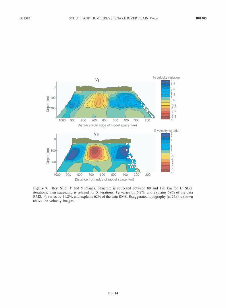
Figure 9. Best SIRT P and S images. Structure is squeezed between 80 and 190 km for 15 SIRTiterations, then squeezing is relaxed for 5 iterations. VP varies by 6.2%, and explains 59% of the dataRMS. VS varies by 11.2%, and explains 62% of the data RMS. Exaggerated topography (at 25x) is shownabove the velocity images.

B01305 SCHUTT AND HUMPHREYS: SNAKE RIVER PLAIN VP/VS B01305

9 of 14

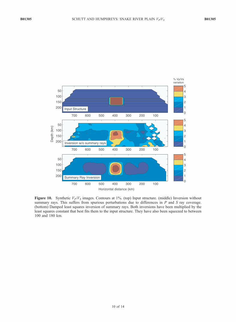
Figure 10. Synthetic VP/VS images. Contours at 1%. (top) Input structure. (middle) Inversion withoutsummary rays. This suffers from spurious perturbations due to differences in P and S ray coverage.(bottom) Damped least squares inversion of summary rays. Both inversions have been multiplied by theleast squares constant that best fits them to the input structure. They have also been squeezed to between100 and 180 km.


10 of 14

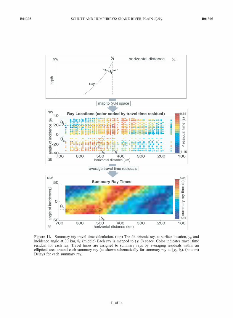
Figure 11. Summary ray travel time calculation. (top) The ith seismic ray, at surface location, yi, andincidence angle at 30 km, qi. (middle) Each ray is mapped to ( y, q) space. Color indicates travel timeresidual for each ray. Travel times are assigned to summary rays by averaging residuals within anelliptical area around each summary ray (as shown schematically for summary ray at ( ys, qs). (bottom)Delays for each summary ray.


11 of 14

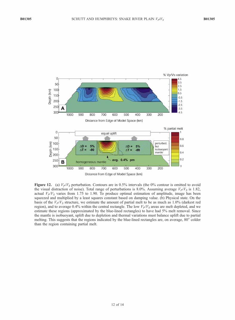
Figure 12. (a) VP/VS perturbation. Contours are in 0.5% intervals (the 0% contour is omitted to avoidthe visual distraction of noise). Total range of perturbations is 8.0%. Assuming average VP/VS is 1.82,actual VP/VS varies from 1.75 to 1.90. To produce optimal estimation of amplitude, image has beensqueezed and multiplied by a least squares constant based on damping value. (b) Physical state. On thebasis of the VP/VS structure, we estimate the amount of partial melt to be as much as 1.0% (darkest redregion), and to average 0.4% within the central rectangle. The low VP/VS areas are melt depleted, and weestimate these regions (approximated by the blue-lined rectangles) to have had 5% melt removal. Sincethe mantle is isobuoyant, uplift due to depletion and thermal variations must balance uplift due to partialmelting. This suggests that the regions indicated by the blue-lined rectangles are, on average, 80� colderthan the region containing partial melt.


12 of 14

Documents

P and S wave velocity and VP/// VS in the wake of the ...cormier/geo_inv5.pdf · S in the wake of the Yellowstone hot spot Derek L. Schutt1 ... 6–10 m.y. B.P. Data are teleseismic