Embed Size (px)
Citation preview

Oxygen Loss from Venus and the Influence of Extreme Solar Wind Conditions
by
Tess Rose McEnulty
A dissertation submitted in partial satisfaction
of the requirements for the degree of
Doctor of Philosophy
in
Earth and Planetary Science
in the
Graduate Division
of the
University of California, Berkeley
Committee in charge:
Professor Imke de Pater, Chair
Dr. Janet G. Luhmann
Professor Walter Alvarez
Professor Stuart Bale
Fall 2012

Oxygen Loss from Venus and the Influence of Extreme Solar Wind Conditions
Copyright 2012
by
Tess Rose McEnulty

1
Abstract
Oxygen Loss from Venus and the Influence of Extreme Solar Wind Conditions
by
Tess Rose McEnulty
Doctor of Philosophy in Earth and Planetary Science
University of California, Berkeley
Professor Imke de Pater, Chair
The purpose of this dissertation is to expand our understanding of oxygen ion
escape to space from Venus and its dependence on extreme solar wind conditions
found during interplanetary coronal mass ejections (ICMEs). This work uses in-situ
measurements of ions and magnetic fields from the Venus Express (VEX)
spacecraft, which has been orbiting Venus since mid-2006. VEX is in a 24 hour
elliptical orbit. The ion instrument operates for ~6 hours near the planet, while the
magnetometer is always on. In-situ measurements of the solar wind velocity,
density, and magnetic field from Pioneer Venus Orbiter (PVO) are also used for
comparison with external conditions during the VEX time period. Coronagraph
images from solar monitoring spacecraft are used to identify the solar sources of the
extreme solar wind measured in-situ at Venus. For interpretation of planetary ions
measured by VEX, a magnetohydrodynamic (MHD) model is utilized.
The solar wind dynamic pressure outside of the Venus bow shock did not exceed
~12 nPa, during 2006-2009, while the solar wind dynamic pressure was higher than
this for ~10% of the time during the PVO mission. Oxygen ions escape Venus
through multiple regions near the planet. One of these regions is the magnetosheath,
where high energy pick-up ions are accelerated by the solar wind convection electric
field. High energy (>1 keV) O+ pick-up ions within the Venus magnetosheath
reached higher energy at lower altitude when the solar wind was disturbed by
ICMEs compared to pick-up ions when the external solar wind was not disturbed,
between 2006-2007. However, the count rate of O+ was not obviously affected by
the ICMEs during this time period. In addition to high energy pick-up ions, VEX
also detects low energy (~10-100 eV) O+ within the ionosphere and wake of Venus.
These low energy oxygen ions are difficult to interpret, because the spacecraft’s
relative velocity and potential can significantly affect the measured energy. If VEX
ion data is not corrected for the spacecraft’s relative velocity and potential,
2
gravitationally bound O+ could be misinterpreted as escaping. These gravitationally
bound oxygen ions can extend on the nightside to ~-2 Venus radii and may even
return to the planet after reaching high altitudes in the wake. Gravitationally bound
ions will lower the total O+ escape estimated from Venus if total escape is calculated
including these ions. However, if the return flux is low compared to the total
escaping outflow, this effect is not significant.
An ICME with a dynamic pressure of 17.6 nPa impacted Venus on November 11,
2011. During this ICME, the high energy pick-up O+ and the low energy O
+ ions
were affected. Oxygen ions in the magnetosheath, ionosphere, and tail had higher
energies during the ICME, compared to O+ energies when the external solar wind
conditions were undisturbed. High energy ions were escaping within the dayside
magnetosheath region when the ICME was passing as well as when the solar wind
was undisturbed. However, during the ICME passage, these O+ ions had three orders
of magnitude higher counts. The low energy O+ during the undisturbed days was
gravitationally bound, while during the ICME a portion of the low energy ions were
likely escaping. The most significant difference in O+ during the ICME was high
energy pickup ions measured in the wake on the outbound portion of the orbit.
These ions had an escape flux of 2.5 108 O
+cm
-2sec
-1, which is higher than the
average escape flux in all regions of the wake. In addition, the interplanetary
magnetic field (IMF) was in a configuration that may have rotated an even higher
escape flux O+ away from the VEX orbit. This needs to be confirmed with
sampling of other regions in the wake during large ICMEs. A lower bound on the
total O+ escape during this event could be ~2.8 10
26 to 6.5 10
27 O
+/sec, which is
2-3 orders of magnitude higher than the average escape flux measured by VEX.
Hence, ICMEs could have played a major role in the total escape of O+ from Venus.
Considering that the Sun was likely more active (with more ICMEs) early after solar
system formation.
The results presented in this dissertation can be used as a guide for future studies of
O+ escape at Venus. As we move into solar maximum, Venus will likely be
impacted by more large ICMEs. The ICME from the last study of this dissertation
was the largest yet measured by VEX, but its 17.6 nPa dynamic pressure is lower
than the largest ICMEs during the PVO time period (~ 80 nPa). The work in this
dissertation is also relevant to Mars, since Mars interacts with the solar wind in a
similar manner and has analogous ion escape mechanisms. The upcoming MAVEN
(Mars Atmosphere and Volatile Evolution) mission will launch at the end of 2013 to
study the Martian atmosphere, escape processes, and history of volatiles. This
mission will have an in-situ ion instrument and magnetometer similar to those used
for the studies in this dissertation, so one could conduct similar studies of the
oxygen ion escape from Mars during extreme solar wind conditions.

i
Dedicated to Bob Lin

ii

iii
Contents
Acknowledgements .................................................................................................. vi
Introduction .............................................................................................................. 1
1.1 Motivation for this dissertation research .......................................................... 1
1.2 Atmospheric escape mechanisms ..................................................................... 4
1.3 Solar wind interaction with Venus .................................................................... 5
1.4 Previous in-situ measurements of solar wind induced O+ escape..................... 6
1.5 Characteristics of the Sun and solar wind ......................................................... 8
1.5.1 The Sun ...................................................................................................... 8
1.5.2 The solar wind .......................................................................................... 10
1.5.3 The solar cycle ......................................................................................... 11
1.5.4 Solar wind disturbances ........................................................................... 12
1.6 Previous studies of solar wind disturbance effect on oxygen ion escape ....... 14
1.7 Dissertation Outline ........................................................................................ 15
Comparing External Conditions That Influence Ion Escape at Venus during
Pioneer Venus and Venus Express Missions ........................................................ 17
2.1 Introduction ..................................................................................................... 18
2.2 Data sets .......................................................................................................... 24

iv
2.3 Statistics of solar wind dynamic pressures, IMF cone angles, and IMF
rotations ................................................................................................................ 25
2.3.1 Solar wind dynamic pressure ................................................................... 26
2.3.2 Cone Angle ............................................................................................... 29
2.3.3 IMF rotations ............................................................................................ 32
2.4 Discussion of results and comparison with other studies ............................... 35
2.5 Possible implications for Venus ion escape rate estimates ............................. 35
2.6 Summary ......................................................................................................... 36
2.7 Future work ..................................................................................................... 37
Interplanetary Coronal Mass Ejection Influence on High Energy Pick-up Ions
at Venus ................................................................................................................... 38
3.1 Introduction ..................................................................................................... 38
3.2 The Venus Solar Wind Interaction ................................................................. 40
3.3 Venus Express ................................................................................................. 43
3.4 Venus Express Data Analysis ......................................................................... 44
3.5 Results ............................................................................................................. 46
3.6 Discussion and Conclusions ........................................................................... 50
Comparisons of Venus Express Measurements with an MHD Model of O+ ion
flows: Implications for Atmosphere Escape Measurements ............................. 55
4.1 Introduction ..................................................................................................... 56
4.2 Description of the MHD model ...................................................................... 57
4.3 Details of VEX IMA, Ion Measurement Complications, and Orbit ............... 61
4.4 Case Studies – validating model, and investigating orbit geometry and IMF
influence ................................................................................................................ 62

v
4.4.1 Validating the model and investigating orbit geometry effect on VEX ion
measurements .................................................................................................... 63
4.4.2 IMF direction effect on ion energy-time spectrograms ............................ 66
4.5 MHD wake geometry, return flows, and escape rate ...................................... 68
4.5.3 Escape flux in model depending on integration region ............................ 73
4.6 Conclusions ..................................................................................................... 77
Chapter 5 ................................................................................................................. 78
Effects of a Large ICME on Oxygen Ion Escape at Venus ................................. 78
5.1 Introduction ..................................................................................................... 78
5.2 November 3, 2011 Coronal Mass Ejection ..................................................... 81
5.3 ICME at Venus ............................................................................................... 82
5.4 O+ detections during the ICME and comparison to an undisturbed orbit ....... 84
5.5 O+ escape during ICME compared to undisturbed orbits ............................... 87
5.6 Conclusions ..................................................................................................... 91
Conclusion ............................................................................................................... 93
6.1 Summary ......................................................................................................... 93
6.2 Major scientific contributions ......................................................................... 94
6.3 Implications for future Venus ion escape studies ........................................... 95
6.4 Future work ..................................................................................................... 96
Bibliography ............................................................................................................ 97
vi
Acknowledgements
Many people have helped me with the work in this dissertation. Thank you to my
advisors, Janet Luhmann and Imke de Pater for all of the time you spent guiding me.
I know that I was not the easiest student to advise, but you kept pushing me to
become a better scientist. Thanks to all of the people that have been coauthors on
my papers (which are part of this dissertation) and conference presentations: Andrei
Fedorov, Yingjuan Ma, Demet Ulusen, Tielong Zhang, Lan Jian, Dave Brain, Edik
Dubinin, Chris Russell, Niklas Edberg, Chris Möstl, and Yoshifumi Futaana. Thank
you to Elizabeth Cappo for proofreading this whole document.
Many scientists and engineers inspired me to pursue a PhD. Thank you to my
undergraduate professor at the University of Michigan, particularly to Nilton Renno
and Alec Gallimore for giving me my first research experiences, and to Thomas
Zurbuchen giving me advice about grad school. Thanks to the people that I worked
for at JPL before grad school that taught me priceless information about space
exploration and inspired me to pursue a PhD (Harold Kirkham, Lynn Baroff, Steve
Fuerstenau, John Crawford, and David Atkinson).
Thank you to the people in the Earth and Planetary Science and Astronomy
departments at Berkeley for giving me a broad understanding of Planetary Science
outside of my specialty, especially Geoff Marcy for organizing interesting CIPS
seminars and giving me the opportunity to be a GSI for his class. Thanks to Bill
Dietrich for teaching an interesting Geomorphology class, and for being on my
qualifying exam committee.
Thanks to all of the scientists and engineers that I interacted with at the Space
Sciences Lab: Dave Brain, Rob Lillis, Christina Lee, Yan Li, Jasper Halekas, Matt
Fillingham, Tim Quinn, Heidi Fuqua, Andrew Poppe, and Rebecca Samad. Special
thanks to Greg Delory for giving me the opportunity to work on the MAVEN LPW
instrument. I really loved getting in the lab building circuits and testing the
instrument. I’m not sure if I would have made it through grad school without this
break from doing data analysis on my computer.

vii
Finally, without my family, friends, and husband I never would have made it to
where I am now. I have been fascinated by space and by the planets for as long as I
can remember. Thank you to my family for always encouraging me. Thank you
mom for the weekly library trips, for making math fun, and for letting me decorate
my room with planets and stars. Thanks dad for always reminding me to stop and
smell the roses. Thanks siblings (Kendra, Cory, Kevin, and Ian). Thanks to my
friends for your support throughout the past few years - especially to Natasha
Chopp, Alyssa Rhoden, Kelly Wiseman, Caroline Chouinard, and Amanda Butina.
Finally, the person I credit most with helping me to finish my PhD: my husband,
Ryan Falor. Words cannot describe how much you have meant to me. You are the
only person that truly knows how hard I worked, and how much I struggled. You
never gave up on me. You pushed me to keep going when I didn’t think that I could
do it anymore. You picked up the slack around the house when I was spending 16
hours a day on my computer focused on my research. Your technical support was
also much appreciated. I am so lucky to have a husband that believes in me as you
do.

viii

1
Chapter 1
Introduction
1.1 Motivation for this dissertation research
Figure 1.1: In the foreground, the surface of Venus revealed by Magellan radar in
1996, and behind it, the planet at visible wavelengths obtained by Pioneer Venus in
1978. (Credit: NASA/JPL/RPIF/DLR)

CHAPTER 1: INTRODUCTION
2
For thousands of years people have watched the Sun, the Moon, the stars, and the
objects that wander among the background stars – the planets. The brightest of these
wanderers was named after goddesses of love: the Babylonian Ishtar, the Greek
Aphrodite, and the Roman Venus. The planet Venus moved from a subject of myth
to that of science after the invention of the telescope. In 1610 Galileo noticed that
Venus exhibited phases similar to the Moon, which supported the theory that the
Sun was the center of the solar system. Details of the planet were further revealed in
1761 when Mikhail Lomonosov, a Russian astronomer, discovered that Venus also
has an atmosphere. This discovery was made during a transit of Venus in front of
the Sun, an event that occurs in pairs separated by long gaps over 100 years. Many
people thought that Venus was likely similar to Earth, and perhaps that there was
even a civilization living on the planet. However, this view of an Earth-like planet
and the historical associations of Venus with beauty and love were completely
overturned during the space age. Close up measurements of the planet, starting with
Mariner 2 in 1963, revealed that it has a hellish environment. It has a crushing CO2
atmosphere, 100 times the surface pressure of Earth, a surface temperature of 736 K
(460° C), and sulfuric acid clouds. Venus is the nearest neighbor to Earth and is
similar in size and internal structure, but it ended up with a very different
atmosphere. Was this always the case, or could Venus have once been much more
Earth-like? A key to answering this question is the history of water on the planet.
Studying Venus can help us understand Earth and Mars, which formed in a similar
location in the solar system. Although these three planets formed in a similar
location (0.7 AU, 1 AU, and 1.5 AU), they are each unique. Venus and Earth are
similar in radius, mass, and distance from the sun (see Table 1.1). However, Venus
does not have an intrinsic dipole magnetic field as the Earth does, and (as mentioned
earlier) has a very different atmosphere. Mars is smaller than both Venus and Earth,
but like Venus, it does not have an intrinsic magnetic field. However, Mars does
have remnant crustal magnetic fields. Another striking difference between these
terrestrial planets is the amount of water. Earth’s surface is covered ~70% by water,
Mars has very little, and Venus is completely dry (only 200-300 ppm in the
atmosphere). Although Venus currently has very little water, this may not have
always been the case. As evidenced by a D/H ratio 100 times that on Earth, Venus
may have actually once had an ocean’s worth of water (Donahue et al., 1982,
McElroy et al. 1982). Mars also has evidence of past water (e.g. Head et al., 1999;

CHAPTER 1: INTRODUCTION
3
Squyres et al., 2004). This dissertation is focused on Venus, but lessons learned can
be applied to Mars.
Venus Earth Mars Radius (km) 6052 6371 3396
Mass (kg) 4.87 1024
5.97 1024
6.42 1023
Intrinsic magnetic field no yes No, but remnant
Distance from Sun (AU) 0.7 1 1.5
Surface pressure 9.3 Mpa 101 kPa ~ 0.6 kPa
Atmosphere
composition
~97% CO2,
~3.5% N2
78% N2,
21% O2
95.3% CO2,
2.7% N2
Escape velocity (km/s) 10.5 11.2 5
Amount of water in
atmosphere
200-300 ppm 1% 210 ppm
Table 1.1: Characteristics of Venus, Earth and Mars. (Amount of water from
Hoffman et al., 1980; Moroz et al., 1979; Johnson and Fegley, 2000)
Water can be lost from Venus if it is photodissociated by solar UV and the hydrogen
escapes to space (e.g. Lammer et al, 2006; Kasting and Pollack, 1983). However,
the leftover oxygen cannot escape to space as easily due to its higher mass. A
mechanism that can impart the energy needed for oxygen to escape to space is
interaction with the interplanetary magnetic fields (IMF) and associated electric
fields in the solar wind (if the oxygen is ionized). Oxygen could also be lost from
the atmosphere due to sequestration in minerals in the crust (e.g. Fegley et al., 2004;
Hashimoto et al., 2008; Smrekar et al., 2011), but this process likely cannot account
for the amount of missing oxygen (Fegley et al., 2004). The study of oxygen
sequestration within the crust is a separate piece of the puzzle. This dissertation
focuses on escape of O+ to space. Estimates of the current O
+ escape rate from
Venus cannot account for the total amount of oxygen expected to have once been on
the planet (e.g. Barabash et al., 2007; Fedorov et al., 2011). However, previous
studies have suggested that the escape rate may increase during extreme conditions
(Luhmann et al., 2007; Futaana et al., 2007; Edberg et al., 2011). In this dissertation,
I further investigate the influence of extreme solar wind conditions on O+ escape to
space.
CHAPTER 1: INTRODUCTION
4
1.2 Atmospheric escape mechanisms
Atmospheric constituents can escape the gravitational bounds of a planet through
mechanisms such as large impacts (e.g. Walker, 1986; Melosh and Vickery, 1989),
Jean’s escape (e.g. Chassefiere, 1996, 1997), photochemistry, or the solar wind
interaction (e.g., Barabash et al., 2007; Terada et al., 2002; Luhmann, 2006, 2007).
Large impacts were probably important shortly after the formation of the solar
system, but the significance of these large impacts would have diminished in ~500
Myr as number and size of impacting bodies were reduced over time. Jean’s escape
and photochemistry at Venus are not capable of accelerating oxygen up to escape
velocity because of its high mass (e.g. Nagy et al., 1981). Therefore, the solar wind
interaction with ionized particles in the upper atmosphere of Venus is likely the
primary mechanism for oxygen loss to space for the past 4 billion years.
The Earth has an internal dynamo magnetic field that holds the solar wind off many
Earth radii, but Venus does not have an internal field. Without a magnetic shield,
the solar wind gets much closer to Venus and interacts directly with its upper
atmosphere and ionosphere. The solar wind carries with it frozen in magnetic fields
as it propagates away from the Sun. The ionosphere of Venus responds to these
magnetic fields. Since charged particles are able to move in the ionosphere they
create an induced magnetic field that holds off the IMF. Outside of this region of
induced magnetic field, neutral particles in the upper atmosphere of Venus can be
ionized and then react with the background magnetic and electric fields. These
ionized particles can be accelerated to velocities above what would be needed for
escape by the pick-up process. The pick-up process is a result of the action of the
solar wind convection electric field (E = -Vsw x B), where Vsw is the velocity of the
bulk solar wind and B is the frozen in interplanetary magnetic field. When an
ionized particle is moving perpendicular to a magnetic field it rotates around the
magnetic field (shown at the top of Figure 1.2). If the magnetic field that the ion is
gyrating around is moving, as with the IMF in the solar wind, the particle will
appear to have a cycloidal motion and be carried away with the moving magnetic
field.

CHAPTER 1: INTRODUCTION
5
Figure 1.2: The pick-up ion process. (top) An ion moving around a stationary
magnetic field (B) moves in a circle around the field. (below) The solar wind carries
frozen in magnetic fields (Bfield) with it, moving with velocity Vsw. As these
magnetic fields move away from the Sun, ions that interact with them move in a
circle around the field, but since the field is moving they appear to have a cycloidal
motion (from Luhmann 2003).
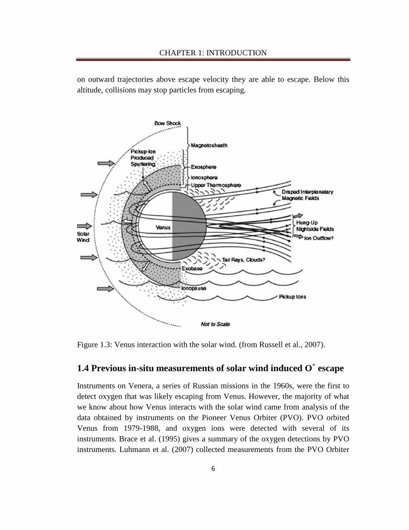
1.3 Solar wind interaction with Venus
The solar wind interacts directly with the ionosphere of Venus (as opposed to the
Earth where the internal dynamo magnetic field holds off the solar wind). This
interaction is illustrated in Figure 1.3. The upper boundary of the ionosphere where
the density quickly falls off is called the ionopause and is usually separated from the
solar wind by the magnetic barrier where IMF piles up and the magnetic pressure
dominates (e.g. Zhang et al., 1991, 2007). The balance between the ionosphere
thermal pressure (which is sensitive to EUV) and solar wind dynamic pressure
determines the location of the ionopause (e.g. Luhmann et al., 1986, 1992). The
magnetosheath is the region above the ionopause where the solar wind IMF is
compressed as it piles up, and where ions are picked up. The exobase is the altitude
at which particles are likely to be collisionless. Above the exobase, if particles are
CHAPTER 1: INTRODUCTION
6
on outward trajectories above escape velocity they are able to escape. Below this
altitude, collisions may stop particles from escaping.
Figure 1.3: Venus interaction with the solar wind. (from Russell et al., 2007).
1.4 Previous in-situ measurements of solar wind induced O+ escape
Instruments on Venera, a series of Russian missions in the 1960s, were the first to
detect oxygen that was likely escaping from Venus. However, the majority of what
we know about how Venus interacts with the solar wind came from analysis of the
data obtained by instruments on the Pioneer Venus Orbiter (PVO). PVO orbited
Venus from 1979-1988, and oxygen ions were detected with several of its
instruments. Brace et al. (1995) gives a summary of the oxygen detections by PVO
instruments. Luhmann et al. (2007) collected measurements from the PVO Orbiter
CHAPTER 1: INTRODUCTION
7
Neutral Mass Spectrometer (ONMS) and modeled features seen in the data as pick-
up ions. Low energy ions were also measured flowing within the ionosphere and
near the ionopause by the ONMS and Ion Mass Spectrometer (IMS) (Knudsen et al.,
1982; Miller and Whitten, 1991; Grebowsky et al., 1993).
Venus Express (VEX) is an orbiter that arrived at Venus in mid-2006, which is
extending the knowledge of ion escape from Venus. It is sampling a region that
PVO did not sample, within -3 Venus radii in the wake behind the planet. VEX has
an instrument called the Ion Mass Analyzer (IMA) which can detect ions within an
energy range of 10 eV - ~25 keV. Statistical studies of the ions detected by the IMA
showed a majority of ions escaping in the wake, rather than through the
magnetosheath (Barabash et al., 2007; Fedorov et al., 2011) The spatial distribution
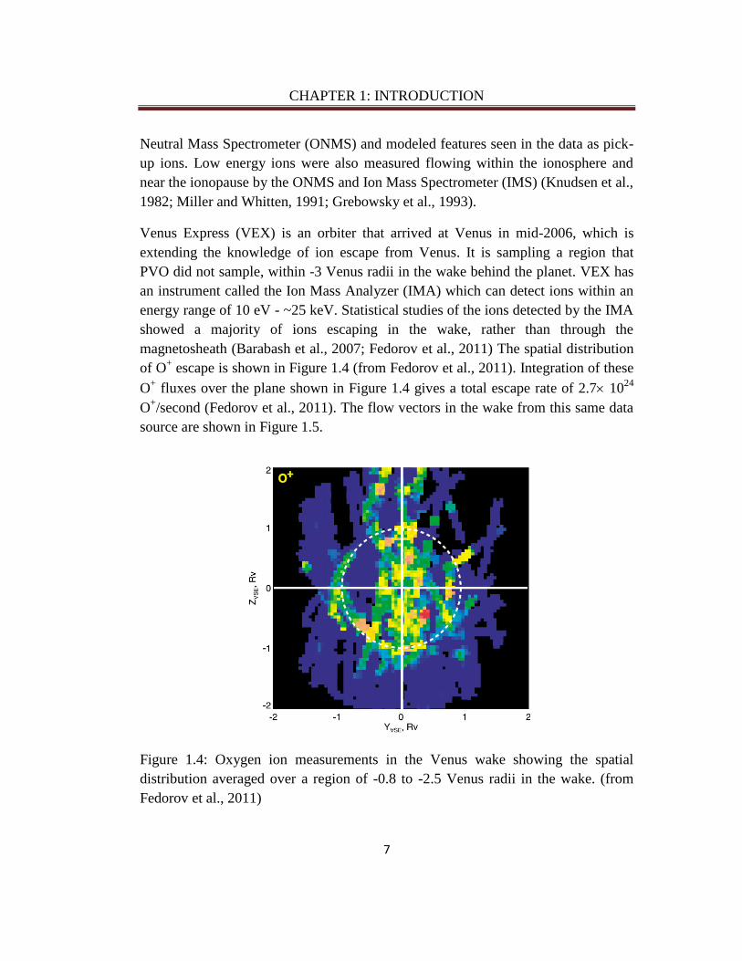
of O+ escape is shown in Figure 1.4 (from Fedorov et al., 2011). Integration of these
O+ fluxes over the plane shown in Figure 1.4 gives a total escape rate of 2.7 10
24
O+/second (Fedorov et al., 2011). The flow vectors in the wake from this same data
source are shown in Figure 1.5.
Figure 1.4: Oxygen ion measurements in the Venus wake showing the spatial
distribution averaged over a region of -0.8 to -2.5 Venus radii in the wake. (from
Fedorov et al., 2011)

CHAPTER 1: INTRODUCTION
8
Figure 1.5: O+ flow vectors averaged from VEX IMA measurements. (from Fedorov
et al., 2011)
1.5 Characteristics of the Sun and solar wind
Conditions on the Sun and in the solar wind can control the Venus-solar wind
interaction, and therefore may affect ion escape. In order to understand how
representative our current measurements of O+ escape rate are of historical values it
is important to consider the Sun and solar wind conditions. In addition to average
conditions on the Sun, we are interested in extreme solar wind conditions that
happen in solar wind disturbances. The Sun, the solar wind, the solar cycle, and
solar disturbances are described further in the following sections.
1.5.1 The Sun
The Sun is a massive ball of plasma (ionized gas), which creates the majority of
energy that we use here on Earth through nuclear fusion of hydrogen to helium in its
CHAPTER 1: INTRODUCTION
9
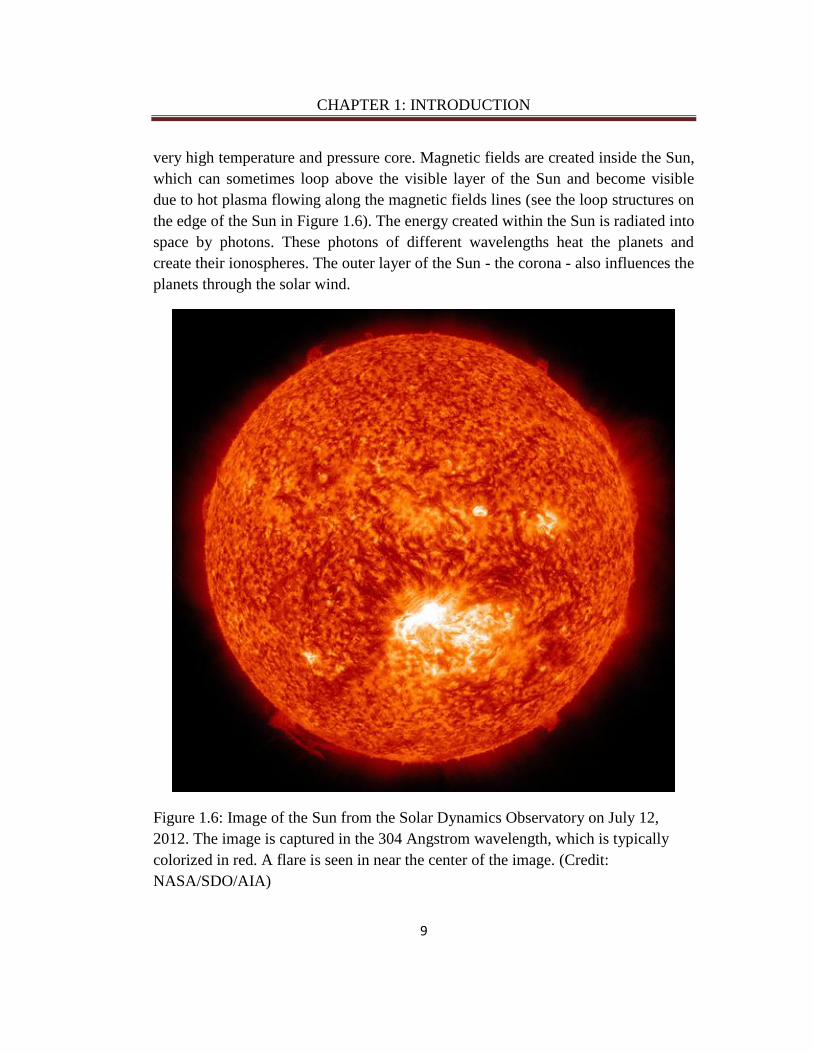
very high temperature and pressure core. Magnetic fields are created inside the Sun,
which can sometimes loop above the visible layer of the Sun and become visible
due to hot plasma flowing along the magnetic fields lines (see the loop structures on
the edge of the Sun in Figure 1.6). The energy created within the Sun is radiated into
space by photons. These photons of different wavelengths heat the planets and
create their ionospheres. The outer layer of the Sun - the corona - also influences the
planets through the solar wind.
Figure 1.6: Image of the Sun from the Solar Dynamics Observatory on July 12,
2012. The image is captured in the 304 Angstrom wavelength, which is typically
colorized in red. A flare is seen in near the center of the image. (Credit:
NASA/SDO/AIA)
CHAPTER 1: INTRODUCTION
10
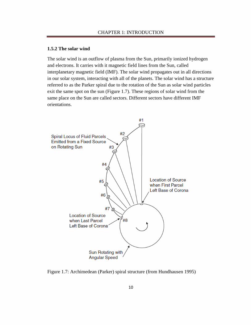
1.5.2 The solar wind
The solar wind is an outflow of plasma from the Sun, primarily ionized hydrogen
and electrons. It carries with it magnetic field lines from the Sun, called
interplanetary magnetic field (IMF). The solar wind propagates out in all directions
in our solar system, interacting with all of the planets. The solar wind has a structure
referred to as the Parker spiral due to the rotation of the Sun as solar wind particles
exit the same spot on the sun (Figure 1.7). These regions of solar wind from the
same place on the Sun are called sectors. Different sectors have different IMF
orientations.
Figure 1.7: Archimedean (Parker) spiral structure (from Hundhausen 1995)
CHAPTER 1: INTRODUCTION
11
1.5.3 The solar cycle
The Sun has an 11-year cycle in which the internal magnetic field flips direction.
Dark spots on the sun (called sunspots) occur where the Sun’s magnetic field loops
above the photosphere of the Sun. The plasma is cooler, within these loops, relative
to the background solar plasma (making them dark). The change in direction of the
internal magnetic field alters the number of sunspots visible on the surface of the
Sun, therefore the sunspot number is a measure of the solar cycle. When the Sun is
most active and has the most sunspots it is considered to be in solar maximum (and
the opposite for solar minimum). The EUV flux is solar cycle dependent with higher
flux at solar maximum compared to minimum by a factor of two (Brace et al., 1988;
Ho et al., 1993). The sunspots are the location of solar flares and coronal mass
ejections discussed in 1.5.4. These solar wind disturbances also depend on the solar
cycle. More disturbances occurring during solar maximum when there are more
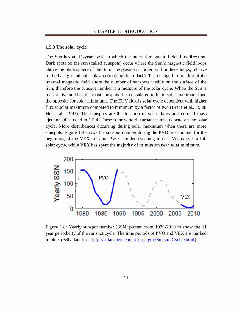
sunspots. Figure 1.8 shows the sunspot number during the PVO mission and for the
beginning of the VEX mission. PVO sampled escaping ions at Venus over a full
solar cycle, while VEX has spent the majority of its mission near solar minimum.
Figure 1.8: Yearly sunspot number (SSN) plotted from 1979-2010 to show the 11
year periodicity of the sunspot cycle. The time periods of PVO and VEX are marked
in blue. (SSN data from http://solarscience.msfc.nasa.gov/SunspotCycle.shtml)
PVO
VEX

CHAPTER 1: INTRODUCTION
12
1.5.4 Solar wind disturbances
Coronal Mass Ejections (CMEs) are outbursts of plasma and twisted magnetic fields
from sunspots (Figure 1.9). They propagate into the ambient solar wind and are
then referred to as ICMES (Interplanetary CMES). ICMEs are characterized by a
leading shock jump and compressed solar wind (high density and dynamic pressure)
followed by a larger than average magnetic field that is smooth and rotating.
Properties of ICMEs are summarized in Jian et al. (2006, 2008). The region of
compression is called the ‘ICME sheath’ (See Figure 1.10).
Figure 1.9: Coronal Mass Ejection (CME) imaged by SOHO LASCO white light
coronagraph (http://cdaw.gsfc.nasa.gov/CME_list/)

CHAPTER 1: INTRODUCTION
13
Figure 1.10: Cartoon of the CME expanding into and affecting the background solar
wind and interplanetary magnetic field. (J.Luhmann, personal comm.)
Stream Interaction Regions (SIRs) occur at sector boundaries where solar wind with
different velocities meet and a higher velocity stream compresses the slower moving
stream ahead of it, as shown in Figure 1.11. SIRs are identified as regions of
enhanced magnetic field and density followed by a high speed solar wind upstream,
as in Jian et al. (2008). They are also called Corotating Interaction Regions (CIRs).

CHAPTER 1: INTRODUCTION
14
Figure 1.11: Stream Interaction Region (SIR) is a compression region where streams
of different solar wind origins meet. (from Pizzo et al., 1991)
1.6 Previous studies of solar wind disturbance effect on oxygen ion
escape
Enhancements of up to 10x in the O+ escape flux were measured by PVO during
periods of high dynamic pressure in ICMEs (Luhmann et al., 2007) (See Figure
1.12). Possible enhancements by 5-10x escape flux during ICMEs were also
reported on VEX (Futaana et al., 2008, Luhmann et al., 2008). Enhanced O+ escape
flux during SIR/ICME passage has been found by Edberg et al. (2011), which
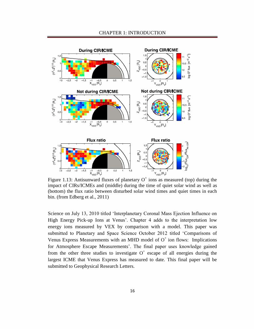
showed a 1.9x enhancement compared to undisturbed solar wind (Figure 1.13). In

CHAPTER 1: INTRODUCTION
15
addition, SIRs with dynamic pressure above the average (1.3 nPa) had 36% more
escape than the lower dynamic pressure SIRs.
Figure 1.12: Suprathermal >36 eV O
+ flux measured by the PVO neutral mass
spectrometer during 1979, compared to the magnetic field magnitude and solar wind
dynamic pressure measured in the upstream solar wind. Vertical lines indicate
where ICMEs were identified. (from Luhmann et al., 2007)
1.7 Dissertation Outline
This dissertation is comprised of four papers, three of which have been published or
are in the review process with the journal Planetary and Space Science, while the
fourth paper will be submitted to the journal Geophysical Research Letters. Chapter
2 compares the external solar wind conditions that VEX encountered from 2006-
2009 to the conditions during the PVO time period. This paper is titled ‘Comparing
External Conditions That Influence Ion Escape at Venus during Pioneer Venus and
Venus Express Missions’, and was submitted to Planetary and Space Science
February 2012, and resubmitted after review and revision on October 2012. The
next study, in Chapter 3, was published in Planetary and Space
CHAPTER 1: INTRODUCTION
16
Figure 1.13: Antisunward fluxes of planetary O
+ ions as measured (top) during the
impact of CIRs/ICMEs and (middle) during the time of quiet solar wind as well as
(bottom) the flux ratio between disturbed solar wind times and quiet times in each
bin. (from Edberg et al., 2011)
Science on July 13, 2010 titled ‘Interplanetary Coronal Mass Ejection Influence on
High Energy Pick-up Ions at Venus’. Chapter 4 adds to the interpretation low
energy ions measured by VEX by comparison with a model. This paper was
submitted to Planetary and Space Science October 2012 titled ‘Comparisons of
Venus Express Measurements with an MHD model of O+ ion flows: Implications
for Atmosphere Escape Measurements’. The final paper uses knowledge gained
from the other three studies to investigate O+ escape of all energies during the
largest ICME that Venus Express has measured to date. This final paper will be
submitted to Geophysical Research Letters.

17
Chapter 2
Comparing External Conditions That Influence Ion Escape
at Venus during Pioneer Venus and Venus Express
Missions
Abstract
Estimates of the oxygen ion escape rate from Pioneer Venus Orbiter (PVO) varied
between 1024
-1026
O+/second. The more recent estimate, from Venus Express
(VEX), is ~2.7*1024
O+/sec. Because of the different instrument calibrations on
PVO and VEX it is difficult to compare escape rates directly. However, VEX will
be making measurements as we move into solar maximum allowing quantification
of certain effects of the solar cycle. We can use the external conditions that PVO
encountered to inform how typical the VEX conditions are compared to other solar
cycles. We are interested in external conditions that influence ion escape (high
dynamic pressure, small cone angles (<30°), and interplanetary magnetic field
rotations). These parameters are considered to affect the ionopause altitude (above
which ions are picked up), mode of ion pickup, and contribution of bulk ionosphere
escape, respectively. Thus, in order to understand variations in escape rates (made
with the same instrument and calibration) we must understand the solar wind setting
of the measurements. In this study, we present yearly histograms of solar wind
dynamic pressure, interplanetary magnetic field cone angles, and interplanetary
magnetic field rotations. We show how these external conditions vary over the full
solar cycle measured by PVO (1979 through 1988) and compare to the external
conditions measured by VEX during the declining to minimum phase of the most
recent cycle (mid 2006 through 2009). The median solar wind dynamic pressure
near Venus during the VEX time period was ~0.5-1.5 nPa compared to ~4-6 nPa
during the PVO time period. Also the VEX time period did not have the extreme
high solar wind dynamic pressures >24 nPa that occurred during the PVO time

CHAPTER 2: EXTERNAL CONDITIONS AT VENUS
18
period. This lack of extreme solar wind dynamic pressures during the VEX time
period is likely caused by the absence of large interplanetary coronal mass ejections.
There was also a lower occurrence of small cone angles (15-20%) during the VEX
time period versus 20-30% during the PVO time period, meaning that the cone
angle was larger during the VEX time period. The VEX time period also had a
higher occurrence of large (>100°) IMF spiral angle rotations than the PVO time
period. The lower dynamic pressure and lower occurrence of small cone angles
during the VEX time period could partially explain a low escape rate measured by
VEX (if the two order of magnitude higher estimates of escape of PVO are actually
representative of real escape rates). We cannot compare these rates directly, but this
result opens up the possibility of higher escape during solar maximum. This will be
measured by VEX over the next few years. The higher occurrence of large IMF
rotations during the VEX time period could make bulk escape more important
during this period compared to the PVO time period. This study illuminates the
complications of interpreting ion escape rates due to the sometimes counteracting
effects of numerous external variables. These do not all follow the same solar cycle
trends and may differ from cycle to cycle, and can be used to inform further study of
detailed ion escape on Venus Express.
2.1 Introduction
The most recent estimate of oxygen ion escape from Venus Express (VEX) is on the
low-end of estimates from Pioneer Venus Orbiter (PVO) (2.7*1024
from Fedorov et
al. (2011) vs 1024
-1026
O+/sec (from e.g., Kasprzak et al, 1991; Brace et al., 1995).
The PVO measurements are from different instruments with different calibration, so
they may not actually represent a real two order of magnitude difference in escape
rate. It is possible that the high-end estimates are inaccurate, but they open up the
possibility that Venus can have a higher escape rate than measured by Fedorov et al.
(2011). It is still an open question of how the total oxygen ion escape varies with the
solar cycle. It may be better answered as Venus Express continues to make
measurements as we go into solar maximum. Measuring the escape rate over the full
current solar cycle still may not be representative of what is possible during other,
more intense, solar cycles. The observations in Fedorov et al. (2011) were from May
24, 2006 to December 12, 2007. This time period was during the declining phase of
solar cycle 23, heading into the weakest solar minimum of the space age (Jian et al.,
2011). It is important to consider the external conditions during the observation
periods, particularly those that might modify escape rates, to put the escape rate
estimates in context and guide further investigation of escape by Venus Express.
External conditions relevant to ion escape include solar extreme ultraviolet (EUV)
flux and solar wind dynamic pressure nv2, where n is density and v is velocity. The

CHAPTER 2: EXTERNAL CONDITIONS AT VENUS
19
balance between the ionosphere thermal pressure (which is sensitive to EUV) and
solar wind dynamic pressure determines how much of the ionosphere will be
exposed to the interplanetary magnetic fields (IMF). which can accelerate ions away
from the planet (e.g. Luhmann et al., 1986, 1992). The upper boundary of the
ionosphere where the density quickly falls off is called the ionopause and it is
usually separated from the solar wind by the magnetic barrier where IMF piles up
and the magnetic pressure dominates (e.g. Zhang et al., 1991, 2007). The
configuration and magnitude of IMF can affect the mechanisms of ion escape,
including ion pickup, ion outflow or bulk escape processes described below. Ion
pick-up is due to the convection electric field in the solar wind E = -v x B, where v
is the solar wind bulk velocity and B is the magnetic field vector (e.g. Luhmann et
al., 2006). Ion pick-up occurs when there are ions created above the ionopause,
which depends on the extension of the neutral exosphere. Observations have also
suggested possible polar wind-like outflows (Hartle and Grebowsky, 1990).
Ionosphere/solar wind boundary intrusions of ionospheric plasma referred to as
“plasma clouds” which may act as a bulk ionosphere removal process from the top
of the ionosphere (e.g. Brace et al., 1982). Lower energy ion outflow may also be
due to the JxB force, where J is current density and B is magnetic field (e.g.
Shinagawa, 1996a,b; Tanaka, 1998).
The EUV flux is solar cycle dependent with higher flux at solar maximum
compared to minimum by a factor of two (Brace et al., 1988; Ho et al., 1993). This
causes higher ionospheric pressure through both ion production and heating (Bauer
and Taylor, 1981). When the Sun is more active, the higher ionospheric pressure
holds off the solar wind plasma and prevents the draped interplanetary magnetic
fields from penetrating into the ionosphere. Under these conditions, cross-terminator
flows supply a nightside ionosphere. During solar minimum when the ionosphere
has lower pressure the draped fields may penetrate the ionosphere, which may shut
off most transterminator flows and cause the nightside ionosphere to disappear (as
proposed by Luhmann and Cravens, 1991). Luhmann et al. (1993) discussed how
higher EUV can lead to enhanced escape of pick-up ions through multiple
mechanisms via a more extended neutral thermosphere, a denser exosphere and a
higher photoionization rate. Moore et al. (1990) and Kasprzak et al. (1991) both
found higher escaping O+ flux measured by PVO during higher solar EUV periods.
The solar wind dynamic pressure (the external control of the ionopause altitude) is
enhanced during the passage of Stream Interaction Regions (SIRs), which are the
structures between fast and slow solar wind streams. This dynamic pressure
enhancement is due to compression between streams as shown in Figure 2.1.
Dynamic pressure is also high in transient events called Interplanetary Coronal
Mass Ejections (ICMEs) as they compress slower solar wind in front of them as

CHAPTER 2: EXTERNAL CONDITIONS AT VENUS
20
shown in Figure 2.2 (reviewed by Crooker et al., 1997). Enhancements of up to
100x in the O+ escape flux measured by PVO during periods of high dynamic
pressure in ICMEs were reported by Luhmann et al. (2007), and possible
enhancements by 5-10x escape flux during ICMEs were also reported on VEX
(Futaana et al., 2008, Luhmann et al., 2008). Enhanced O+ escape flux during SIR
passage has been found by Edberg et al. (2011) which showed a 1.9 times
enhancement compared to undisturbed solar wind. Edberg et al. (2011) also
investigated the effect of dynamic pressure. They did this by sorting SIR cases by
dynamic pressure into bins higher or lower than the median of 1.3 nPa and found
that the higher dynamic pressure SIRs had 36% more escape than the lower
dynamic pressure SIRs.
Figure 2.1: Stream Interaction Region (SIR) due to a faster solar wind stream
running into a slower stream and causing a compression region in front and a
rarefaction region behind it, from Pizzo (1978).

CHAPTER 2: EXTERNAL CONDITIONS AT VENUS
21
Figure 2.2: ICME expanding into the solar wind and compressing solar wind in
front of it which leads to higher dynamic pressure.
Even within undisturbed solar wind, the velocity is variable due to diverse source
regions on the sun, and this can lead to different orientations of the IMF based on
the theory of Parker (1963), which explains the average spiral configuration of the
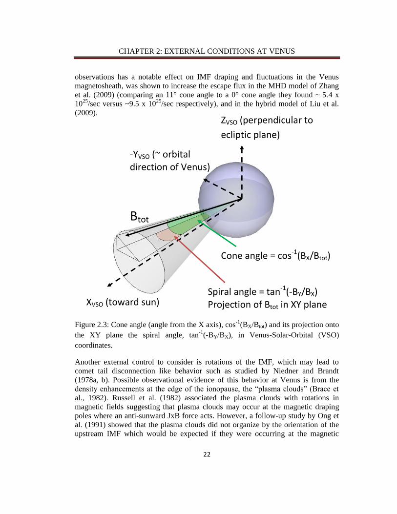
IMF in the ecliptic, depends on solar wind velocity. The angle of the field in the
ecliptic, the IMF spiral angle shown in Figure 2.3, is measured from the line radial
to the sun in the orbital plane of Venus given by tan-1
(-BY/BX). Here BY and BX are
IMF vector components in Venus-Solar-Orbital (VSO) coordinates (where X is
toward the sun, Z is perpendicular to the ecliptic, and Y completes the right hand
system). At Venus the average spiral angle is ~36°. The IMF is not always in the
ecliptic and includes the BZ component which gives the cone angle cos-1
(Bx/Btot) as
shown in Figure 2.3. The cone angle has not been definitively shown to affect the
ion escape rate in data analysis but was shown to possibly affect the ion escape
mechanisms in VEX ion data by Masunaga et al. (2011). Low cone angle, which in
CHAPTER 2: EXTERNAL CONDITIONS AT VENUS
22
observations has a notable effect on IMF draping and fluctuations in the Venus
magnetosheath, was shown to increase the escape flux in the MHD model of Zhang
et al. (2009) (comparing an 11° cone angle to a 0° cone angle they found ~ 5.4 x
1025
/sec versus ~9.5 x 1025
/sec respectively), and in the hybrid model of Liu et al.
(2009).
Figure 2.3: Cone angle (angle from the X axis), cos-1
(BX/Btot) and its projection onto
the XY plane the spiral angle, tan-1
(-BY/BX), in Venus-Solar-Orbital (VSO)
coordinates.
Another external control to consider is rotations of the IMF, which may lead to
comet tail disconnection like behavior such as studied by Niedner and Brandt
(1978a, b). Possible observational evidence of this behavior at Venus is from the
density enhancements at the edge of the ionopause, the “plasma clouds” (Brace et
al., 1982). Russell et al. (1982) associated the plasma clouds with rotations in
magnetic fields suggesting that plasma clouds may occur at the magnetic draping
poles where an anti-sunward JxB force acts. However, a follow-up study by Ong et
al. (1991) showed that the plasma clouds did not organize by the orientation of the
upstream IMF which would be expected if they were occurring at the magnetic
ZVSO (perpendicular to
ecliptic plane)
Cone angle = cos-1(BX/Btot)
Btot
Spiral angle = tan-1(-BY/BX) Projection of Btot in XY plane XVSO (toward sun)
-YVSO (~ orbital direction of Venus)

CHAPTER 2: EXTERNAL CONDITIONS AT VENUS
23
draping poles. Instead they found that the magnetic field rotations may have been
external rotations in the IMF. The average clock angle rotation of the IMF inbound
versus outbound on orbits that had clouds was 59°, compared to the average solar
wind rotation of 29°. The average solar wind rotation in their study for comparison
with the orbits containing clouds was calculated between points separated by 75
minutes, the approximate time between inbound and outbound crossings of the bow
shock. If the plasma clouds are a bulk removal process, they may contribute
significantly to the total escape flux with an estimated 1025
-1026
O+/second (Russell
et al., 1982; Brace et al., 1982). IMF rotations may also have contributed to the 1.9
times enhanced ion escape flux measured by VEX during SIRs by Edberg et al.
(2011) because SIRs are often associated with heliospheric current sheet (HCS)
crossings, which separate inward versus outward IMF field lines (e.g. Gosling et al.,
1978; Jian et al., 2006).
In this paper we consider solar wind characteristics that may be associated with
enhanced escape flux: high dynamic pressures, small cone angles, and large IMF
rotations. We study the occurrence of these solar wind conditions during the full
solar cycle that PVO sampled (January 1979-August 1988) and the declining to
minimum phase of VEX measurements (June 2006 through 2009). The solar cycle
sampling of the time periods in this study is shown in Figure 2.4. Our results
provide a summary of what solar wind and IMF conditions VEX has encountered
that may affect the measured escape flux. The comparisons with PVO era
counterparts suggest possible reasons, other than the solar EUV flux, that might
affect differences in escape rate.
Figure 2.4: Solar cycle setting of PVO and VEX. SSN is sunspot number. (SSN data
from http://solarscience.msfc.nasa.gov/SunspotCycle.shtml)
PVO
VEX

CHAPTER 2: EXTERNAL CONDITIONS AT VENUS
24
2.2 Data sets
For the VEX solar wind and interplanetary magnetic field statistics that we present
in this paper, we use data from the ASPERA-4 Ion Mass Analyzer (IMA) (Barabash
et al., 2007) and magnetometer (Zhang et al., 2006) during June 2006 through the
end of 2009. VEX has a highly elliptical ~24 hour orbit with periapsis near the
northern pole of Venus and the line joining periapsis and apoapsis nearly
perpendicular to the ecliptic so that periapsis always samples near the north pole.
The magnetometer makes continuous observations, while the IMA makes
measurements primarily within a few hours of periapsis. We use 10 minute
resolution for both datasets and restrict the available measurements to upstream of
the Venus bow shock, in order to sample the solar wind rather than the planetary
region. We used the bow shock equations from Zhang et al. (2008) where r is in
Venus Radii: r = 2.14/ (1+0.621*cos (SZA)) for SZA<=117° and r = 2.364/sin
(SZA+10.5°) for SZA > 117°. The solar wind data set is highly restricted, because
the IMA instrument is normally operated for only a few hours near periapsis (out of
the ~24 hour orbit) and most of this near periapsis data is not used (due to being
within the bow shock). To derive the solar wind dynamic pressure we use VEX
IMA density and velocity from the AMDA website (http://cdpp-
amda.cesr.fr/DDHTML/index.html). The VEX IMA is not a dedicated solar wind
monitor, and can become saturated in the solar wind, so we only use measurements
with a high quality, and compare the calculated dynamic pressure to measurements
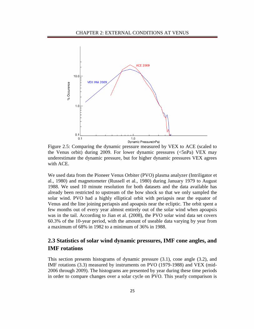
made by the ACE spacecraft. Figure 2.5 shows a comparison of the % occurrence of
dynamic pressure in 2009 measured by the VEX IMA and ACE. VEX may saturate
and may underestimate dynamic pressures <5nPa, but is able to measure higher
dynamic pressures similar to the ACE solar wind monitor, which are the pressures
of primary interest in this paper.
CHAPTER 2: EXTERNAL CONDITIONS AT VENUS
25
Figure 2.5: Comparing the dynamic pressure measured by VEX to ACE (scaled to
the Venus orbit) during 2009. For lower dynamic pressures (<5nPa) VEX may
underestimate the dynamic pressure, but for higher dynamic pressures VEX agrees
with ACE.
We used data from the Pioneer Venus Orbiter (PVO) plasma analyzer (Intriligator et
al., 1980) and magnetometer (Russell et al., 1980) during January 1979 to August
1988. We used 10 minute resolution for both datasets and the data available has
already been restricted to upstream of the bow shock so that we only sampled the
solar wind. PVO had a highly elliptical orbit with periapsis near the equator of
Venus and the line joining periapsis and apoapsis near the ecliptic. The orbit spent a
few months out of every year almost entirely out of the solar wind when apoapsis
was in the tail. According to Jian et al. (2008), the PVO solar wind data set covers
60.3% of the 10-year period, with the amount of useable data varying by year from
a maximum of 68% in 1982 to a minimum of 36% in 1988.
2.3 Statistics of solar wind dynamic pressures, IMF cone angles, and
IMF rotations
This section presents histograms of dynamic pressure (3.1), cone angle (3.2), and
IMF rotations (3.3) measured by instruments on PVO (1979-1988) and VEX (mid-
2006 through 2009). The histograms are presented by year during these time periods
in order to compare changes over a solar cycle on PVO. This yearly comparison is

CHAPTER 2: EXTERNAL CONDITIONS AT VENUS
26
useful because published escape rate estimates have used data from differing time
periods on PVO and VEX. It can guide future studies of the ion escape during
different time periods. For each section comparing PVO to VEX the histogram bins
on the x axis are the same and the number of data points in each bin is normalized
by the total number of data points, so that the distributions can be compared
directly.
2.3.1 Solar wind dynamic pressure
Histograms of the solar wind dynamic pressure by year over the PVO time period
are shown in Figure 2.7. The last bin of this histogram (24 nPa) includes all
measurements above that value. The peak of the main solar wind dynamic pressure
distribution during the PVO time period was lowest during solar maximum (~1980)
and highest near solar minimum (~1985-1986). This agrees with previous statistics
of the solar wind dynamic pressure on PVO showing an average of 4.5 nPa at solar
maximum and 6.6 nPa at solar minimum (e.g. Luhmann et al., 1993; Russell et al.,
2006). Histograms of solar wind dynamic pressure by year from VEX are shown in
Figure 2.6 from the declining phase into solar minimum in 2009, which does not
have the same trend. The dynamic pressure peak was highest during 2006 during the
declining phase and lowest during 2009 during minimum.
Figure 2.6: Histograms of solar wind dynamic pressure broken up by year measured
by VEX.
% O
ccu
rren
ce

CHAPTER 2: EXTERNAL CONDITIONS AT VENUS
27
Figure 2.7: Histograms of solar wind dynamic pressure broken up by year measured
by PVO (where the last bin includes all data above 24 nPa). These histograms show
how the solar wind dynamic pressure distribution changed over the solar cycle on
PVO and how the solar wind dynamic pressure was much higher during the PVO
time period than the VEX time period (shown in Figure 2.6).
% O
ccu
rren
ce

CHAPTER 2: EXTERNAL CONDITIONS AT VENUS
28
The median dynamic pressure during the PVO time period was significantly higher
than during the VEX time period (~4-6 nPa compared to ~0.5-1.5 nPa). Another
difference is that the PVO time period had a high dynamic pressure tail above 24
nPa that is not seen in the VEX data. The high dynamic pressure tail (>24 nPa) was
likely due to ICMEs during the PVO time period as shown in the bottom panel of
Figure 2.8. In this figure the red ICME distribution makes up the higher occurrence
rate of dynamic pressures above 24 nPa. For more information about the
characteristics of ICMEs on PVO see Jian et al. (2008).
Figure 2.8: Comparing the characteristics of ICMEs and SIRs to solar wind on
PVO.

CHAPTER 2: EXTERNAL CONDITIONS AT VENUS
29
2.3.2 Cone Angle
Histograms of the IMF cone angle by year from 1979-1988 from PVO are shown in
Figure 2.10, and for the VEX time period (mid 2006-2009) in Figure 2.9. The
background color separates small (<30° or >150°), intermediate (30°-60° or 120°-
150°) and large (60°-120°) cone angles. These angle bins were chosen because they
are the ranges used by Masunaga et al. (2011). These histograms show a change in
the shape of the cone angle distribution by year, with the PVO distributions taking
on a more saddle-like shape. This means that there are less large cone angles shown
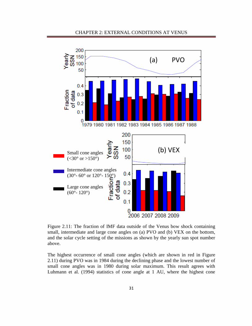
in the gray background sections. In order to better quantify the total contribution of
small cone angles by year and to more easily compare PVO to VEX, we summed
the % occurrence in the small, intermediate and large bins each year, with the results
shown in Figure 2.11.
Figure 2.9: Cone angle, cos-1
(BX/Btot), histograms of % occurrence by year during
VEX (mid-2006-2009). Background color corresponds to cone angle ranges
described as small (light red), intermediate (light blue), and large (gray).
Cone angle separated bins:
Small (<30° or >150°)
Intermediate (30°- 60° or 120°- 150°)
Large (60°- 120°)

CHAPTER 2: EXTERNAL CONDITIONS AT VENUS
30
Figure 2.10: Cone angle, cos-1
(BX/Btot), histograms of % occurrence by year during
PVO 1979-1988. Background color corresponds to cone angle ranges described as
small (light red), intermediate (light blue), and large (gray).
CHAPTER 2: EXTERNAL CONDITIONS AT VENUS
31
Figure 2.11: The fraction of IMF data outside of the Venus bow shock containing
small, intermediate and large cone angles on (a) PVO and (b) VEX on the bottom,
and the solar cycle setting of the missions as shown by the yearly sun spot number
above.
The highest occurrence of small cone angles (which are shown in red in Figure
2.11) during PVO was in 1984 during the declining phase and the lowest number of
small cone angles was in 1980 during solar maximum. This result agrees with
Luhmann et al. (1994) statistics of cone angle at 1 AU, where the highest cone
(a) PVO
(b) VEX Small cone angles
(<30° or >150°)
Intermediate cone angles
(30°- 60° or 120°- 150°)
Large cone angles
(60°- 120°)

CHAPTER 2: EXTERNAL CONDITIONS AT VENUS
32
angles occurred during solar maximum (1980) and the lowest during the declining
period. For the VEX time period in Figure 2.9b the lowest number of small cone
angles was in 2009 during solar minimum, which is the opposite of the PVO trend.
Comparing VEX to PVO, the occurrence of small cone angles (<30°) was less
during the solar minimum period of VEX during 2009 (15%) versus PVO during
1986 (30%). This would imply that the solar wind velocity was lower during the
VEX period, which agrees with Jian et al. (2011) who showed that at 1 AU the
average solar velocity in 1986 was 459 km/s while in July 2008-June 2009 it was
388 km/s.
2.3.3 IMF rotations
Ong et al. (1991) found that the possible bulk removal plasma clouds measured by
PVO occurred more often when there was a large rotation of the IMF. Many of
these rotations may have been due to crossing the heliospheric current sheet (HCS)
since the current sheet separates inward versus outward spiral interplanetary
magnetic field (Schulz 1973). These different sectors of magnetic field orientation
can be seen in magnetic field spiral angle time series as period. The spiral angle
stays near the same positive or negative value for a time period and then rotates in
sign and stays at that new value, making a checkerboard-like pattern as shown in
Figure 2.12. The frequency of rotations is due to the warp of the HCS which varies
over the solar cycle, introducing more variations when the current sheet is
everywhere near the ecliptic (e.g. Hoeksema et al., 1983).
Figure 2.12: Time series of IMF spiral angle showing sector boundaries measured
by VEX near Venus.

CHAPTER 2: EXTERNAL CONDITIONS AT VENUS
33
Figure 2.13: Time series of IMF spiral angle showing sector boundaries measured
by PVO near Venus.
The occurrence of IMF rotations are shown as histograms of spiral angle rotation
calculated between data points separated by 10 minutes in Figure 2.14b for PVO
and Figure 2.14a for VEX. The majority of the IMF rotation angles during both
PVO and VEX time periods changed by less than 20° every 10 minutes. Comparing
PVO to VEX there are more large rotations in the VEX data as seen by the tail in

CHAPTER 2: EXTERNAL CONDITIONS AT VENUS
34
the spiral angle rotation histogram above 100°. This is absent in the PVO data
except in 1985-1986 which had some high rotation occurrence (but not as high as
any of the VEX years).
Figure 2.14: Histograms by year of spiral angle rotations on (a) VEX (2006-2009)
and (b) PVO (1979-1988).
(b) PVO
(a) VEX
% O
ccu
rren
ce
% O
ccu
rren
ce

CHAPTER 2: EXTERNAL CONDITIONS AT VENUS
35
2.4 Discussion of results and comparison with other studies
The Venus Express results come from the declining phase into an unusually long
and deep solar minimum (e.g. McComas et al., 2008; Lee et al. 2009; Jian et al.,
2011). Lee et al. (2009) showed that this declining phase (February 4-November 4,
2007) had unusually low density at 1 AU compared to a similar solar cycle sample
during the previous cycle (February 23-November 22, 1995). Jian et al. (2011)
extended this result to the two previous solar minimums in 1976 and 1986, showing
that the most recent minimum is the weakest of the four periods studied.
Our statistics of this most recent period show weak solar wind dynamic pressure
compared to the PVO time period, which agrees with the Lee et al. (2009) results of
lower density and with the Jian et al. (2011) results of lower density and lower
dynamic pressure. In particular, Jian et al. (2011) point out that that at 1 AU the
dynamic pressure was ~1.4 nPa in July 2008-June 2009, while it was ~2.97 nPa in
1986, which would have been during the solar minimum of our PVO analysis. Our
results show a high dynamic pressure (>24 nPa) tail on the PVO dynamic pressure
histograms which we attribute to stronger ICMEs during this time period. ICMEs at
Venus during the PVO time period did have high dynamic pressures with a median
dynamic pressure maximum of 20.7 nPa with some extending up to 82 nPa (Jian et
al., 2008). Jian et al. (2011) looked at ICMEs at 1 AU during the most recent
minimum versus the previous minimum in1996, and found that the most recent
minimum has weaker dynamic pressure ICMEs with shorter duration, but there is
not a comparison of the ICMEs during the PVO time period.
Although PVO had higher dynamic pressures, the portion of the dynamic pressure
histograms presented in this study that lead to enhanced escape may depend on the
EUV which is solar cycle dependent. Therefore, the EUV is also important to
consider. Phillips et al. (1984) showed that during solar maximum the peak
ionosphere pressure was around 6 nPa. The PVO data shows that the solar wind
dynamic pressure would have often reached values higher than this, while during
VEX the dynamic pressure was much lower but the EUV was also lower due to
VEX measuring near solar minimum.
2.5 Possible implications for Venus ion escape rate estimates
Our study shows that during the time period we looked at (2006-2009) VEX had not
yet sampled the high dynamic pressure tail of the distribution of pressures seen by
PVO. The 100 times enhancement in O+ flux seen by Luhmann et al. (2007)
occurred at ICME arrivals when the dynamic pressure was above 20 nPa, and our
CHAPTER 2: EXTERNAL CONDITIONS AT VENUS
36
analysis shows that these high pressures occurred ~2-3% of the time on PVO, but
have not happened on VEX (or at least have not happened with an occurrence of
more than 0.1% of the time). This could significantly lower the estimated escape
rate from VEX compared to PVO (although instrument differences on the missions
make this direct comparison between VEX and PVO escape rates difficult to
confirm).
Small cone angles (<30 degrees) occur between 15% and 30% of the time, so if the
cone angle is associated with an increased (or decreased) escape flux of O+ it is
important to take into consideration when comparing escape rates from different
time periods. Depending on if/how cone angle affects the flux; the large amount of
time spent in this IMF configuration could significantly modify the estimates of
escape. We saw less small cone angles on VEX, so it is important to consider if the
cone angle is found to modify escape rates.
IMF rotations may be important drivers of escape if they are associated with the
plasma clouds seen by PVO as suggested by Ong et al. (1991). It is important to
consider this possible escape mechanism when estimating escape rates, particularly
if orbits during which there is a rotation are screened out of the estimates (such as in
Fedorov et al., 2011). Orbits with large rotations are often discarded when looking
at escape because in order to put measurements in a frame considering the
convection electric field. If the IMF is rotating and the spacecraft is downstream of
the bow shock it is hard to estimate the external convection electric field.
Therefore, further work must identify whether or not the IMF rotations are
associated with bulk escape and if so consider them in the total escape flux estimate.
2.6 Summary
1. Dynamic pressure was significantly higher during the PVO time period (in
general and high pressure tail due to ICMEs).
2. VEX dynamic pressure was lowest during 2009 (minimum) which doesn’t agree
with PVO where the lowest dynamic pressure was in 1980 (maximum).
3. VEX had less small cone angle (<30°) occurence compared to the PVO time
period (15-20% versus 20-30%).
4. Small cone angles still happen in a large portion of the time (15-30%) and thus
are important to consider when estimating ion escape rates.
5. VEX had more large (>100°) IMF rotations than the PVO time period.

CHAPTER 2: EXTERNAL CONDITIONS AT VENUS
37
2.7 Future work
There is still not clear consensus on how the O+ ion escape rate from Venus varies
with solar cycle and with changing external conditions. In order to understand this
we must understand the mechanisms of escape and how the escape flux depends on
the external conditions. In particular, additional studies on the cone angle influence
on escape flux and whether plasma clouds are a bulk escape process related to IMF
rotations. Also, measurements of escape during enhanced dynamic pressure by VEX
should be continued as the solar activity picks up and the planet encounters ICMEs
with higher dynamic pressure. All of these measurements must keep the external
conditions in mind, which we have presented in this study.
38
Chapter 3
Interplanetary Coronal Mass Ejection Influence on High
Energy Pick-up Ions at Venus
Abstract
We have used the Ion Mass Analyzer (IMA) and Magnetometer (MAG) on Venus
Express (VEX) to study escaping O+ during Interplanetary Coronal Mass Ejections
(ICMEs). Data from 389 VEX orbits during 2006 and 2007 revealed 265 samples of
high energy pick-up ion features in 197 separate orbits. Magnetometer data during
the same time period showed 17 ICMEs. The interplanetary conditions associated
with the ICMEs clearly accelerate the pickup ions to higher energies at lower
altitudes compared to undisturbed solar wind. However, there is no clear
dependence of the pickup ion flux on ICMEs. This may be attributed to the fact that
this study used data from a period of low solar activity, when ICMEs are slow and
weak relative to solar maximum. Alternatively, atmospheric escape rates may not be
significantly changed during ICME events.
3.1 Introduction
There may have been an ocean’s worth of water on Venus early in its history, as
evidenced by a D/H ratio 100 times that on Earth (Donahue et al., 1982, McElroy et
al. 1982). We must question what happened to the ocean, because Venus’s
atmosphere currently contains little water vapor, only 200-300 ppm (Hoffman et al.,
1980; Johnson and Fegley, 2000). Water vapor can be photodissociated by solar UV
when it reaches a high enough altitude in the atmosphere. After dissociation, it is
possible to lose the hydrogen to space via hydrodynamic escape (Kasting and
CHAPTER 3: ICME INFLUENCE ON HIGH ENERGY PICK-UP IONS
39
Pollack, 1983), but getting rid of the heavier oxygen is more difficult. A portion of
the oxygen may have been taken up by oxidation of the crust (e.g. Fegley et al.,
1997), but this process cannot account for the amount of oxygen that is missing
from the atmosphere (Lewis and Kreimendahl, 1980). Oxygen can be lost if it is
ionized and stripped away by the solar wind.
The lack of an internal dipole magnetic field allows direct scavenging of ionized
atmospheric constituents from the atmosphere of Venus by the solar wind (e.g.,
Barabash et al., 2007a; Terada et al., 2002; Luhmann, 2006, 2007). Oxygen ion
escape has been observed on both Pioneer Venus Orbiter (PVO) and Venus Express
(VEX), respectively described in Luhmann et al. (2006) and Barabash et al. (2007a).
Estimates of the average escape rates of oxygen on Venus range from 1024
s−1
to
1026
s−1
(cf Jarvinen et al., 2009). Atmospheric loss during the first billion years
after planetary formation would have been primarily been due to large impacts. If
subsequent escape (over the next 3.5 billion years) occurred at rates similar to the
present day, the total escape of oxygen would be 1041
to 1043
total oxygen atoms. An
Earth-like ocean contains 1045
water molecules or the equivalent number of oxygen
atoms. Thus the currently observed average escape rates of O+ are insufficient to
account for an ocean’s worth of oxygen loss. In addition, the current escape rate also
includes oxygen from dissociated CO2, so to account for the total oxygen loss from
water you would need an even higher current escape rate. However, conditions in
the solar system have also changed over time, including the Sun and its outputs
which may have affected the total escape of oxygen. In particular, stellar analogs
suggest the early Sun had both higher EUV fluxes and was more active (Newkirk,
1980; Zahnle and Walker, 1982; Lammer et al, 2003) This paper describes a further
contribution to the study of solar activity effects on the escaping oxygen ions at
Venus, as observed on VEX.
Understanding the solar wind induced escape at Venus is also important for
understanding Mars. Since Mars is also unmagnetized it interacts with the solar
wind similarly to Venus on the large scale but is more complicated because of its
small size and remnant crustal magnetic fields. Escape of atmosphere on Mars is
interesting because there is evidence that there was once surface water in liquid
form (e.g. Head et al., 1999; Squyres et al., 2004) which would have required a
thicker atmosphere to cause a greenhouse effect sufficient to warm the surface
above the freezing point of water.
CHAPTER 3: ICME INFLUENCE ON HIGH ENERGY PICK-UP IONS
40
The solar wind induced escape of high energy O+ from Mars has been investigated
by Dubinin et al. (2006). They found a linear dependence of ion energy on altitude
which was attributed to acceleration in an electric field. Dubinin et al (2006) also
noticed that ions in one orbit gained energy more rapidly with altitude than for other
orbits. Using data from the Mars Global Surveyor spacecraft we confirmed that this
particular case where the ions gained energy closer to the planet occurred during a
solar wind disturbance. This study builds on the results of Dubinin et al (2006) with
a survey of more MEX ion data and a similar energy altitude analysis at Venus.
3.2 The Venus Solar Wind Interaction
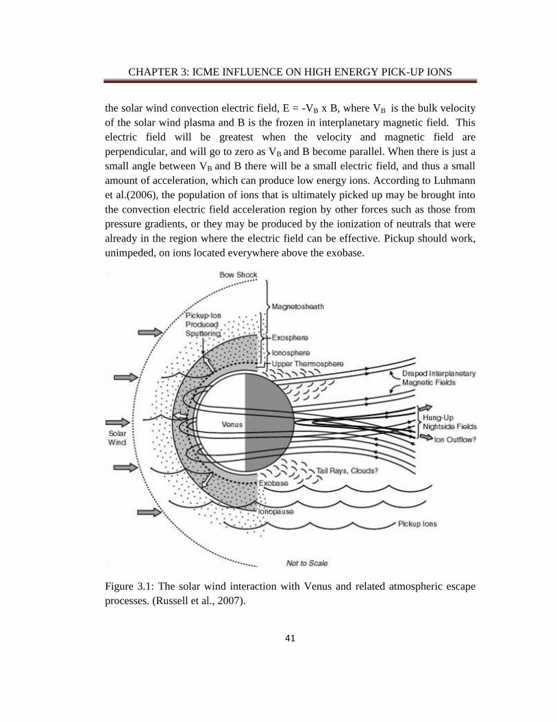
The interaction of Venus with the solar wind is illustrated in Figure 3.1. Since
Venus does not have a dynamo magnetic field, but has an ionosphere, it acts like a
conducting sphere in this solar wind plasma (e.g. Luhmann, 1986). Around solar
maximum, when PVO was at Venus sampling the ionosphere in-situ, the solar wind
and interplanetary magnetic fields did not generally penetrate the ionospheric
obstacle. The field lines drape around and slip over the ionospheric obstacle, frozen
in the largely deflected solar wind. There is a collisionless bow shock that heats and
deflects the solar wind, followed by a region where the solar wind is compressed
and deflected around the ionospheric obstacle. The interplanetary magnetic fields
pile up near the planet. The inner portion of this pile up region is known as the
magnetic barrier or the magnetic pile-up region. The magnetic barrier interfaces
with the main ionosphere at the ionopause current layer that forms between them. A
comet-like tail of draped interplanetary fields is found in the solar wind wake
downstream of the planet. This feature is called an induced magnetotail because it
does not consist of fields of planetary origin like Earth’s magnetotail. Zhang et al.
(2007) refers to the regions near Venus and its wake in which magnetic pressure
dominates the other pressure contributions, which includes both the magnetic barrier
and the magnetotail, as the induced magnetosphere.
Proposed mechanisms for solar wind removal of O+ ions include “ionospheric ion
outflow” possibly connected to polarization electric fields (e.g., Barabash et al.,
2007a) or “bulk ionospheric escape” related to macroscopic or fluid-like instabilities
at the ionopause (e.g., Terada et al., 2002). However, many features of ion escape
seen in PVO have been reproduced in models solely based on the pick-up ion
process (e.g.Luhmann 2006, 2007). The pick-up process is a result of the action of
CHAPTER 3: ICME INFLUENCE ON HIGH ENERGY PICK-UP IONS
41
the solar wind convection electric field, E = -VB x B, where VB is the bulk velocity
of the solar wind plasma and B is the frozen in interplanetary magnetic field. This
electric field will be greatest when the velocity and magnetic field are
perpendicular, and will go to zero as VB and B become parallel. When there is just a
small angle between VB and B there will be a small electric field, and thus a small
amount of acceleration, which can produce low energy ions. According to Luhmann
et al.(2006), the population of ions that is ultimately picked up may be brought into
the convection electric field acceleration region by other forces such as those from
pressure gradients, or they may be produced by the ionization of neutrals that were
already in the region where the electric field can be effective. Pickup should work,
unimpeded, on ions located everywhere above the exobase.
Figure 3.1: The solar wind interaction with Venus and related atmospheric escape
processes. (Russell et al., 2007).
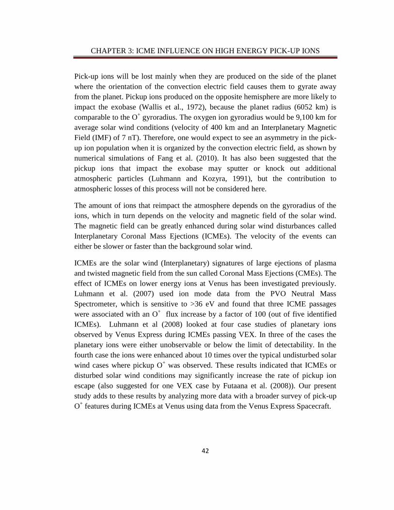
CHAPTER 3: ICME INFLUENCE ON HIGH ENERGY PICK-UP IONS
42
Pick-up ions will be lost mainly when they are produced on the side of the planet
where the orientation of the convection electric field causes them to gyrate away
from the planet. Pickup ions produced on the opposite hemisphere are more likely to
impact the exobase (Wallis et al., 1972), because the planet radius (6052 km) is
comparable to the O+ gyroradius. The oxygen ion gyroradius would be 9,100 km for
average solar wind conditions (velocity of 400 km and an Interplanetary Magnetic
Field (IMF) of 7 nT). Therefore, one would expect to see an asymmetry in the pick-
up ion population when it is organized by the convection electric field, as shown by
numerical simulations of Fang et al. (2010). It has also been suggested that the
pickup ions that impact the exobase may sputter or knock out additional
atmospheric particles (Luhmann and Kozyra, 1991), but the contribution to
atmospheric losses of this process will not be considered here.
The amount of ions that reimpact the atmosphere depends on the gyroradius of the
ions, which in turn depends on the velocity and magnetic field of the solar wind.
The magnetic field can be greatly enhanced during solar wind disturbances called
Interplanetary Coronal Mass Ejections (ICMEs). The velocity of the events can
either be slower or faster than the background solar wind.
ICMEs are the solar wind (Interplanetary) signatures of large ejections of plasma
and twisted magnetic field from the sun called Coronal Mass Ejections (CMEs). The
effect of ICMEs on lower energy ions at Venus has been investigated previously.
Luhmann et al. (2007) used ion mode data from the PVO Neutral Mass
Spectrometer, which is sensitive to >36 eV and found that three ICME passages
were associated with an O+ flux increase by a factor of 100 (out of five identified
ICMEs). Luhmann et al (2008) looked at four case studies of planetary ions
observed by Venus Express during ICMEs passing VEX. In three of the cases the
planetary ions were either unobservable or below the limit of detectability. In the
fourth case the ions were enhanced about 10 times over the typical undisturbed solar
wind cases where pickup O+ was observed. These results indicated that ICMEs or
disturbed solar wind conditions may significantly increase the rate of pickup ion
escape (also suggested for one VEX case by Futaana et al. (2008)). Our present
study adds to these results by analyzing more data with a broader survey of pick-up
O+ features during ICMEs at Venus using data from the Venus Express Spacecraft.

CHAPTER 3: ICME INFLUENCE ON HIGH ENERGY PICK-UP IONS
43
3.3 Venus Express
Venus Express arrived at Venus in April, 2006 and started operations on July 4,
2006. The science mission is planned to last until the end of 2012. It has a 24 hour
elliptical polar orbit with an apoapsis of 66,000 km and a periapsis of 250 km. To
study the interaction of the solar wind with Venus, the spacecraft has a suite of
plasma instruments called ASPERA-4 (Analyzer of Space Plasmas and Energetic
Atoms) and a magnetometer. ASPERA-4 includes an electron spectrometer, two
energetic neutral atom (ENA) sensors, and the ion mass analyzer (IMA) which was
used in this study. The instrument design is based on ASPERA-3 on MEX
(Barabash et al., 2006). IMA makes measurements between 10 eV and 30 keV for
the main ion components H+, He++, He+, O+, and the group of molecular ions 20–
80 amu/q. The IMA instantaneous field of view is 4.6° × 360°, but electrostatic
sweeping performs elevation (±45°) coverage. ASPERA pointing generally includes
the direction of the sun as part of its sampling sequence.
The IMA sweeps through the energy range over 96 steps, with sampling time for
each energy step is 125 ms. The “mass image” of 16 azimuthal sectors × 32 rings
(mass) is read-out once per sampling time. After each complete energy sweep the
instrument changes the elevation angle of the field of view, which is broken into 16
sections. The total 3D sweep (32 rings (mass) × 16 azimuthal sectors × 96 energy
steps × 16 elevation angles) takes 192 seconds. More details of the ASPERA-4
instrument are given in (Barabash et al., 2007b).
The ion mass spectrometer data can be plotted in energy time spectrograms, such as
in Figure 3.2. These plots show the integrated ion counts over a specified mass
range as a function of time and energy. This particular spectrogram was made over
masses of 12-60 amu. The detections you see on the left are background solar wind.
Then, the energy range of the detections broadens. This is due to passing through
the bow shock near the planet. Gaps in detections of ions occur in the energy-time
spectrograms when the instrument is looking away from the sun, because both the
solar wind and planetary ions flow in the anti-solar direction.
An example of pickup ions seen in an energy-time spectrogram is shown circled
Figure 3.2. These features have been referred to as “ion beams” (e.g. Carlsson et al.,
2006). When the spacecraft intersects ions accelerating away from the planet it
detects discrete ion features at sequences of increasing energies along the spacecraft

CHAPTER 3: ICME INFLUENCE ON HIGH ENERGY PICK-UP IONS
44
orbit. Similar features have also been found around Mars by Phobos-2 and Mars
Express (MEX) (Carlsson et al., 2006; Dubinin et al. 2006). Carlsson et al (2006)
showed the composition of the pickup ion beams, at Mars, was primarily O+
and
O2+.
Figure 3.2: Example VEX energy-time spectrogram for high mass ions showing
pick-up ion ‘‘beam’’ detections circled in yellow.
The magnetometer is a dual triaxial fluxgate magnetometer where one triad is used
to correct the measurements for the spacecraft-generated magnetic fields. (Zhang et
al., 2006). It has a large dynamic range between +- 32.8 and +- 8388.6 nT, and
sampling is at up to 128 vectors/second.
3.4 Venus Express Data Analysis
In the present analysis, IMA data were plotted in energy time spectrograms, as in
Figure 3.2, for 389 orbits between 2006-05-20 and 2007-06-13. These spectrograms
were then visually scanned for high energy ion beam features. Beam features were
identified in 197 of the orbits. The criteria for identifying beams were that high
mass ions were seen at energies above that of the solar wind background or below
but with a quasi-linear increase in energy over time. These beams were then
investigated to ensure that they were O+ by plotting mass vs. energy. The example
in Figure 3.3 shows ion mass and energy of ion detections with the counts integrated
over a certain time interval when a beam was seen. The increased counts at higher
mass can be O+, O2
+ or other high mass ions. However, they are most likely O
+
because it has a lower mass and is thus escapes more easily.
Pick-up ions
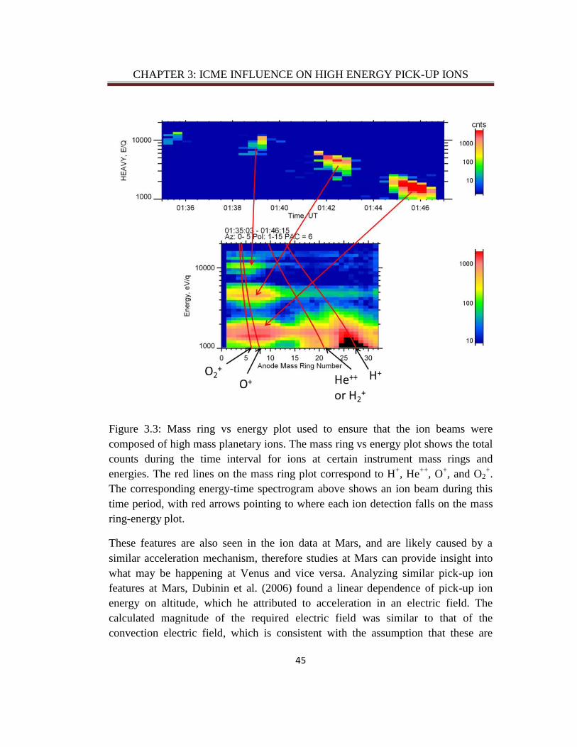
CHAPTER 3: ICME INFLUENCE ON HIGH ENERGY PICK-UP IONS
45
Figure 3.3: Mass ring vs energy plot used to ensure that the ion beams were
composed of high mass planetary ions. The mass ring vs energy plot shows the total
counts during the time interval for ions at certain instrument mass rings and
energies. The red lines on the mass ring plot correspond to H+, He
++, O
+, and O2
+.
The corresponding energy-time spectrogram above shows an ion beam during this
time period, with red arrows pointing to where each ion detection falls on the mass
ring-energy plot.
These features are also seen in the ion data at Mars, and are likely caused by a
similar acceleration mechanism, therefore studies at Mars can provide insight into
what may be happening at Venus and vice versa. Analyzing similar pick-up ion
features at Mars, Dubinin et al. (2006) found a linear dependence of pick-up ion
energy on altitude, which he attributed to acceleration in an electric field. The
calculated magnitude of the required electric field was similar to that of the
convection electric field, which is consistent with the assumption that these are

CHAPTER 3: ICME INFLUENCE ON HIGH ENERGY PICK-UP IONS
46
pick-up ions. Dubinin et al. (2006) also observed that one of the beams had
decreasing energy with altitude, which was also consistent with acceleration in the
convection electric field. However, in this case the ion started in the hemisphere in
which the electric field was directed toward the planet. Dubinin et al (2006) also
noticed that beams in one of the orbits ions gained energy more rapidly with altitude
than for other orbit than the rest which he thought was due to an enhanced solar
wind period, we confirmed this using MGS data.
For our study, looking at the ion beams at Venus we were able to use magnetometer
data to determine when the solar wind was disturbed for all of our ion beams.
Example magnetometer data from September 10-12, 2006 is shown in Figure 3.4,
which shows higher magnetic field near Venus periapsis, because of the pile-up of
the interplanetary magnetic field lines around the planet and what the undisturbed
IMF looks like. This also shows what an ICME looks like. The data were visually
scanned for these standard ICME signatures, including a leading shock jump and
compressed solar wind followed by larger than average ‘ejecta’ magnetic field that
is smooth and rotating (e.g. Luhmann et al., 2008). Most of the ICMEs were around
1-2 days in duration. In addition, IMA moment data, obtained by integrating over
all angles and energies, show high densities and temperatures in the post-shock
sheath due to compression and shock heating. The velocity usually declines during
passage of the ICME. The temperature can be abnormally low after the sheath.
ICMEs are identified according to the characteristics from Jian et al. (2006) and Jian
et al. (2008). The dates of the identified ICMEs are shown in Table 3.1.
3.5 Results
The energies of the detected ion beams are plotted in Figure 3.5 as a function of
altitude, showing a quasi-linear relationship. As Dubinin et al. (2006) pointed out
for the counterpart Mars observations; this behavior likely corresponds to
acceleration of the planetary ions due to the solar wind convection electric field.
Dubinin et al (2006) stated that the highest slope sequence of beam detections in
their Mars cases were likely due to enhanced ion energization from the passage of a
solar wind disturbance and our results confirm this assertion. In Figure 3.5, the
ICME cases are enclosed in diamonds. The ICME cases show higher slopes,
meaning that the ions gain energy faster as the altitude increases. This is not
surprising because the magnetic field in ICMEs is higher than under normal solar
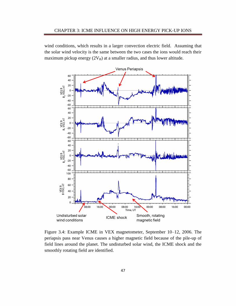
CHAPTER 3: ICME INFLUENCE ON HIGH ENERGY PICK-UP IONS
47
wind conditions, which results in a larger convection electric field. Assuming that
the solar wind velocity is the same between the two cases the ions would reach their
maximum pickup energy (2VB) at a smaller radius, and thus lower altitude.
Figure 3.4: Example ICME in VEX magnetometer, September 10–12, 2006. The
periapsis pass near Venus causes a higher magnetic field because of the pile-up of
field lines around the planet. The undisturbed solar wind, the ICME shock and the
smoothly rotating field are identified.

CHAPTER 3: ICME INFLUENCE ON HIGH ENERGY PICK-UP IONS
48
Table 3.1: ICMEs identified during this study (June 2006–July 2007).
We examined the count rates for each event integrated over the detection interval in
the disturbed and the non-disturbed cases. Since we are interested in the relative
differences between disturbed and non-disturbed cases, the absolute magnitude of
flux in physical units was not necessary to plot. As shown in Figure 3.5, the count
rate does not clearly differ between the ICME cases and the others. The main
organization of the count rate appears to be by altitude of the detections.

CHAPTER 3: ICME INFLUENCE ON HIGH ENERGY PICK-UP IONS
49
Figure 3.5: Pick-up ion detections plotted with color corresponding to
log(counts/sec). ICME cases have diamonds around them. The colors are not
significantly different for ICME cases, which means there is no clear correlation
between count rate and ICMEs.
The orbital locations of each of the beam detections are shown in Figure 3.6. The x-
axis points toward the sun, the y-axis is along the planets orbit in the opposite
direction to planetary motion and the z-axis points northward to complete the right
handed set. In general, the shape of the orbit plots is due to the orbital sampling.
The lack of detections in the +ZVSO hemisphere is due to the orbital sampling. The
energy coded plots show that the ions are gaining energy as they move away from
Venus. The count rate plots show that the highest count rates are close to the planet.
Some of these ions close to the planet may still reimpact the atmosphere so the
count rates measurements aren’t necessarily measuring the escape flux.
Previous analysis by Luhmann et al. (2006) on PVO data and Barabash et al.
(2007a) on Venus Express data has shown that high energy (> 4 keV) planetary ions
are organized by the convection electric field, consistent with a pick-up ion
interpretation. This convection electric field control is established by rotating the
orbital locations of the ion detections according to where the convection electric

CHAPTER 3: ICME INFLUENCE ON HIGH ENERGY PICK-UP IONS
50
field was pointing during the detection. This rotated frame is called the VSE
coordinate system in which +X is toward the sun, and the convection electric field (-
VB x B) in the + Z direction. The orientation of the IMF was determined from the
magnetic field sampled closest to the beam detection outside of the bow shock.
Cases where the IMF changed by>40 degrees, were not considered, because the
IMF measured outside the bow shock may not be reliable during the times that the
beams were detected if it was rapidly changing. Figure 3.7 shows the asymmetry
expected for pick-up ions, and is consistent with the earlier results (e.g. Fang et al,
2010).
3.6 Discussion and Conclusions
This analysis showed that, for the period analyzed, ICMEs clearly influence the
energization of pick-up ion beams at Venus, their effects on the total escape rate is
not clear. This may be due to the strength of the ICMEs encountered during this
study. The period of the VEX measurements in relation to the solar activity
(sunspot) cycle is shown in Figure 8, while the dates of the identified ICMEs are
shown in Table 1. All of the ICMEs for which the solar source has been identified
have been slow (~250 km/s), as is typical for events occurring in the declining and
minimum phase of the solar cycle (Figure 3.8). For comparison, large events during
solar maximum which can range from 800 km/s up to ~2500 km/s (Cane and
Richardson, 2003).
A possible cause for the ICME events that did not result in larger pickup ion fluxes
may be that the observed particles for the ICMEs and the undisturbed solar wind
conditions came from different source regions. Also, an important parameter for
evaluating the flux dependence, for total ion escape rate, may be the ion gyroradius
which is proportional to VB/B. When the magnetic field is higher the gyroradius is
smaller, so more ions may reimpact the atmosphere and not escape. However, when
the velocity is higher the opposite is true. Large values of VB are necessary for
enhancing the ion gyroradius and thus the fraction of total pickup ion escape. An
increased solar wind velocity creates a larger gyroradius so more ions may be able
to be picked up without reimpacting the atmosphere. We do not yet have a good
sample of major solar events in the VEX observations.

CHAPTER 3: ICME INFLUENCE ON HIGH ENERGY PICK-UP IONS
51
Figure 3.6: (left) VEX VSO orbit plots color coded according to log(energy), (right)
VEX VSO orbit plots color coded according to log(counts/sec) showing ICME
cases in diamonds. Going from top to bottom the orbital views are from the side of
the planet(X–Z plane), from the sun (Y–Z plane) and from the top (X–Y plane).
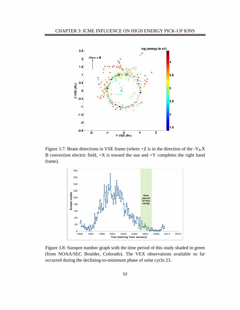
CHAPTER 3: ICME INFLUENCE ON HIGH ENERGY PICK-UP IONS
52
Figure 3.7: Beam detections in VSE frame (where +Z is in the direction of the -VB X
B convection electric field, +X is toward the sun and +Y completes the right hand
frame).
Figure 3.8: Sunspot number graph with the time period of this study shaded in green
(from NOAA/SEC Boulder, Colorado). The VEX observations available so far
occurred during the declining-to-minimum phase of solar cycle 23.
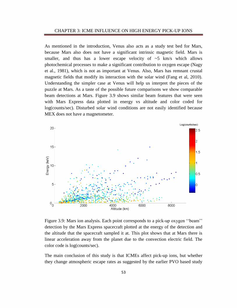
CHAPTER 3: ICME INFLUENCE ON HIGH ENERGY PICK-UP IONS
53
As mentioned in the introduction, Venus also acts as a study test bed for Mars,
because Mars also does not have a significant intrinsic magnetic field. Mars is
smaller, and thus has a lower escape velocity of ~5 km/s which allows
photochemical processes to make a significant contribution to oxygen escape (Nagy
et al., 1981), which is not as important at Venus. Also, Mars has remnant crustal
magnetic fields that modify its interaction with the solar wind (Fang et al, 2010).
Understanding the simpler case at Venus will help us interpret the pieces of the
puzzle at Mars. As a taste of the possible future comparisons we show comparable
beam detections at Mars. Figure 3.9 shows similar beam features that were seen
with Mars Express data plotted in energy vs altitude and color coded for
log(counts/sec). Disturbed solar wind conditions are not easily identified because
MEX does not have a magnetometer.
Figure 3.9: Mars ion analysis. Each point corresponds to a pick-up oxygen ‘‘beam’’
detection by the Mars Express spacecraft plotted at the energy of the detection and
the altitude that the spacecraft sampled it at. This plot shows that at Mars there is
linear acceleration away from the planet due to the convection electric field. The
color code is log(counts/sec).
The main conclusion of this study is that ICMEs affect pick-up ions, but whether
they change atmospheric escape rates as suggested by the earlier PVO based study

CHAPTER 3: ICME INFLUENCE ON HIGH ENERGY PICK-UP IONS
54
is still to be determined. This will influence how we think about early Venus and
early Mars, because the early active sun possibly produced more ICMEs as well as
higher EUV (Lammer et al, 2003). Further characterization of the escape rate of
oxygen with modeling and data analysis of ICMEs during the upcoming solar
maximum will help us answer this question. In addition, a new mission to Mars
called MAVEN will investigate planetary pick-up ion escape further and will
include a solar wind plasma analyzer and a magnetometer. (Jakosky et al., 2008)
55
Chapter 4
Comparisons of Venus Express Measurements with an
MHD Model of O+ ion flows: Implications for Atmosphere
Escape Measurements
Abstract
Low energy (< 100 eV) oxygen ions flowing into the Venusian wake have been
detected by the Venus Express Ion Mass Analyzer, but the spacecraft potential and
relative velocity complicate the interpretation of these ions. We use a
magnetohydrodynamic model to illustrate how Venus Express ion measurements
can be affected by these complications. We simulate Venus Express energy-time
spectrograms with the model by including the spacecraft relative velocity and
potential. Our results illustrate that the shape of the simulated spectrograms depends
on orbit geometry and interplanetary magnetic field direction. Our results facilitate
better orbit-to-orbit comparisons of Venus Express ion data than can be done with
the current ion data. We also address the question of whether the Venus Express
orbit biases statistics of total oxygen escape. We show the global picture of the
wake in the model, and calculate the oxygen ion escape rate that would be inferred.
This is based on averaging the oxygen ion flux measured along the Venus Express
2006-2007 orbits, which were used for published Venus Express escape estimates.
In the model, a region on the nightside contains ions turning back toward the planet
out to 3000 km in the wake. Despite this flow geometry, the escape rate estimates
calculated by averaging along the Venus Express orbit are still within 25% of the
actual total escape from the model. We then look at the escape in the model
calculated along the 2009 and 2010 Venus Express orbits (when the periapsis was
lowered), and find that the estimated escape rate is still within ~20% of the actual
escape from the model. Therefore, return ion flows like those in the MHD model
wake would not significantly affect Venus Express escape rate estimates.

CHAPTER 4: COMPARING VEX ION MEASUREMENTS TO MHD MODEL
56
4.1 Introduction
Venus does not have an intrinsic magnetic field, thus the solar wind interacts
directly with the planet’s upper atmosphere (e.g. Luhmann and Bauer, 1992). The
solar wind carries with it the magnetic field of the sun and sets up electric fields that
can accelerate ionized atmospheric particles to velocities above that needed to
escape from the gravitational field of the planet (e.g., Luhmann, 1986; Russell et al.,
2006). Instruments on Venera, Pioneer Venus Orbiter (PVO), and Venus Express
(VEX) detected ionized hydrogen and oxygen at distances and with energies high
enough to indicate that they were escaping (e.g., Vaisberg et al., 1995; Brace et al.,
1995; Barabash et al., 2007a; Fedorov et al., 2011). Understanding escape
processes, quantifying the current escape rates of H+ and O
+, and determining how
escape depends on external conditions are crucial to ascertain how much water may
have once been on Venus. In order to estimate the escape rate using in-situ
measurements from spacecraft, ion measurements made at one location and time
have to be statistically assembled into a global picture. This step can be facilitated
by using models to provide the context of single orbit measurements. In this paper,
we use a magnetohydrodynamic (MHD) model as a tool to interpret VEX ion
measurements within the ionosphere and wake. MHD models cannot represent high-
energy pick-up ion beams, such as those presented in McEnulty et al. (2010), but
Venus Express investigators claim that the majority of escape is happening at low
energies and within the regions that we explore with the model in this paper (e.g.
Barabash et al., 2007a; Fedorov et al., 2011; Lundin et al., 2011).
Instruments on PVO also measured ions flowing within the ionosphere and into the
wake (e.g., Brace et al., 1995). The Retarding Potential Analyzer (RPA) measured
ionospheric flows across the terminator between 200 and 1000 km altitude at
velocities between 2-5 km/sec, with transient velocities up to 8 km/sec (Knudsen et
al., 1981; Miller and Whitten 1991). Above the ionopause - the boundary between
the ionosphere and solar wind – the Ion Mass Spectrometer (IMS) and the Neutral
Mass Spectrometer (NMS) detected ions with velocity above what would be needed
to escape (Grebowsky et al., 1993; Kasprzak et al., 1991). Brace et al. (1995)
suggested that the RPA flows were higher than needed to maintain the nightside
ionosphere with the implication that some of it may have also escaped. Indeed the
Orbiter Neutral Mass Spectrometer (ONMS) detected O+ ions with >36 eV energies
and antisunward velocities in the low altitude wake (Kasprzak et al., 1991;
Luhmann et al., 2007) even though details of the ion population from this
instrument are limited. Measurements made by the Ion Mass Analyzer (IMA) on
VEX are within the energy range needed to investigate the transition to escape
velocity and better understand the processes controlling escape in these regions.
However, the spacecraft’s relative velocity and potential make these measurements

CHAPTER 4: COMPARING VEX ION MEASUREMENTS TO MHD MODEL
57
difficult to interpret. In order to shed light on these complications, we use an MHD
model to illustrate how the spacecraft relative velocity and potential can affect the
energy of ions measured within VEX orbits.
Models are also useful for exploring the global picture and how the orbital bias of
measurements can affect the amount of escape inferred. The latest estimate of ion
escape using VEX ion statistics by Fedorov et al. (2011) motivates our investigation
of the orbital bias; in particular, measurements as close to the center of the planet as
1.2 Venus Radii (Rv) were used in the statistics. Fedorov et al. (2011) said that past
1.2 Rv in the wake the flow is laminar and the total outflow from the planet is
conserved and does not depend on the distance. However, this laminar conserved
flow is called into question by the results of Lundin et al. (2011) who presented ion
statistics within the wake and said that oxygen ions are gravitationally bound out to
6000 km altitude (2 Rv) in the wake. In this paper, we use an MHD model to
interpret VEX IMA measurements. Section 2 describes some details of the MHD
model used here and its input conditions and section 3 discusses the VEX orbit and
IMA sampling. Case studies and applications to escape measurements are
respectively presented in sections 4 and 5 to illustrate the interpretive value of the
model and its implications.
4.2 Description of the MHD model
In order to create a general picture of the solar wind interaction with the Venus
ionosphere, and in particular the outflowing ions measured by VEX, we use an
MHD model. This model is similar to those described for Mars (Ma et al., 2004a,
2007) and Titan (Ma et al., 2004b). The model has a spherical grid with an inner
boundary at 100 km altitude and a graduated radial grid resolution of 5 km (at the
lower boundary, in the ionosphere) to 600 km. It is single-fluid, multi-species MHD
model utilizing the BATS-R-US (Block Adaptive Tree Solar Wind Roe-Type
Upwind Scheme) code described in Powell et al. (1999). A self-consistent
ionosphere is included with four major ion species (H+, O
+, O2
+ and CO2
+).
Atmospheric neutral profiles and ionization rates are based on Fox et al. (2001).
Solar minimum EUV conditions were assumed, which are appropriate for most of
the VEX observations up to late 2009. The model also includes self-consistent mass
loading and ion-neutral collision effects. Many details about the model development
and numerical treatments of the Venus ionospheric obstacle can be found in the
paper by Ma et al (2012).
The external solar wind description used in the model version for solar minimum is
based on Pioneer Venus Orbiter (PVO) measurements of average solar minimum

CHAPTER 4: COMPARING VEX ION MEASUREMENTS TO MHD MODEL
58
solar plasma and field conditions at Venus from Luhmann et al. (1993): solar wind
density = 22/cc, solar wind velocity = 420 km/s, total magnetic field = 9.6nT, solar
wind temperature = 3.0E5 K. The solar wind flow is in the -X direction, and the
interplanetary magnetic field (IMF) is in the XY plane with a spiral angle, tan-1
(-
BY/BX), of 36°. The convection electric field (E = -V X B where V is the bulk
velocity and B is the IMF vector) is in the +Z direction. This model frame of
reference is similar to the VSE (Venus Solar Electric) frame, which is used to
organize Venus Express data, in that ZVSE is parallel to the convection electric field
and XVSE is antiparallel to the solar wind bulk velocity vector. Our VEX orbit data
are in VSO coordinates where Xvso also points sunward, and the +Yvso axis is in
the direction opposite from planetary orbital motion. For our purposes, we assume
that the model coordinate system is equivalent to VSO coordinates. We also point
out that because the model assumes a single fluid velocity even though it has
multiple species it does not contain convection electric field related asymmetries
related to ion mass except in an averaged sense. We assume this is adequate for our
analysis because we are focusing on the low energy ions whose gyroradii are
generally small compared to the overall solar wind interaction.
The basic model results that we use to study the O+ flows are illustrated by the
contour plots and vectors in Figures 4.1 and 4.2. These show the model O+ and H
+
densities and velocity magnitude as contours with normalized velocity vector
overlays in the terminator plane (Figure 4.1) and the noon-midnight meridian plane
(Figure 4.2). The H+ panels (Figures 4.1b and 4.2b) are dominated by the solar wind
external flows in the magnetosheath and shown for context, while the O+ represents
the ionosphere contribution. The velocity vectors are the same in all plots because
the model is calculated from single fluid MHD. One can see from these two model
cuts that the appearance of the ion fluxes sampled along simulated VEX fly-
throughs will be different depending on the VEX orbit phase with respect to the
Sun and IMF direction. For example, the O+ extends to higher altitudes in the noon-
midnight plane (which intersects the nominal tail plasma sheet region) than in the
terminator plane. In the terminator plan, the magnetic field draping geometry limits
the altitude of the ionopause.
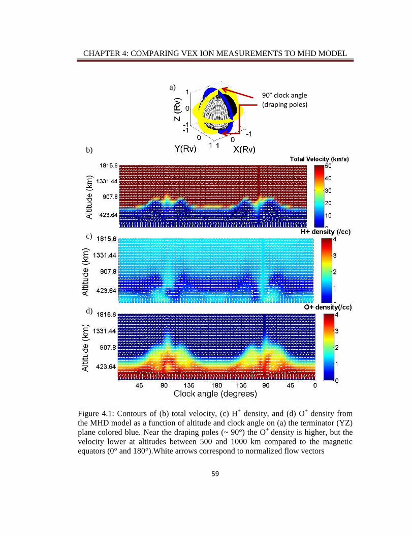
CHAPTER 4: COMPARING VEX ION MEASUREMENTS TO MHD MODEL
59
Figure 4.1: Contours of (b) total velocity, (c) H+ density, and (d) O
+ density from
the MHD model as a function of altitude and clock angle on (a) the terminator (YZ)
plane colored blue. Near the draping poles (~ 90°) the O+
density is higher, but the
velocity lower at altitudes between 500 and 1000 km compared to the magnetic
equators (0° and 180°).White arrows correspond to normalized flow vectors
d)
c)
b)
a) 90° clock angle (draping poles)

CHAPTER 4: COMPARING VEX ION MEASUREMENTS TO MHD MODEL
60
Figure 4.2: Contours of (b) total velocity, (c) H+ density, and (d) O
+ density from
the MHD model as a function of altitude and solar zenith angle on (a) the noon-
midnight (XZ) plane colored blue. 180° SZA is midnight, so the middle of the plots
corresponds to the wake. White arrows correspond to normalized flow vectors,
which turn back toward the planet near midnight.
d)
c)
b)
a)
0° SZA
180° SZA
90° SZA (draping poles)

CHAPTER 4: COMPARING VEX ION MEASUREMENTS TO MHD MODEL
61
4.3 Details of VEX IMA, Ion Measurement Complications, and
Orbit
The Venus Express in-situ Ion Mass Analyzer is part of the suite of instruments
called ASPERA-4 (Analyzer of Space Plasmas and Energetic Atoms) detailed in
Barabash et al. (2007b). The IMA separates ions by mass allowing investigators to
distinguish between hydrogen and heavier ions, such as O+ and O2
+, with an energy
range of 10 eV – 20 keV and energy resolution of 8% within the instantaneous field
of view 4.6° × 360°. The instrument sweeps electrostatically to ±45° in elevation.
The spacecraft body partially blocks this field of view, and the amount of the ion
distribution that is blocked depends on the orientation of the spacecraft.
IMA measurements of ion energy are affected by the relative velocity of the
spacecraft and by the spacecraft potential. These issues are particularly important to
consider when analyzing data at the low end of the energy range. The spacecraft
velocity at periapsis is ~10 km/s (which corresponds to a possible increase of ~10
eV to the measured ions) and the negative (mostly in the night side of Venus)
spacecraft potential may upshift the ion energies by nearly the same magnitude (~5-
10 eV). In order to determine the actual velocity of the measured ions, the spacecraft
relative velocity must be subtracted vectorially and the measured energy shifted
down by the spacecraft potential (the negative potential measured in volts shifts
positive ions up in energy by that magnitude in eV). The potential is not always well
characterized, making some orbits unusable for escape flux statistics. This type of
correction for the spacecraft relative velocity and potential is described in detail by
Fraenz et al. (2010) using a similar instrument on Mars Express.
The orbit of VEX is highly elliptical and polar with a period of 24 hours. Until
August 2008, the periapsis altitude was ~300 km and was then lowered to ~185 km,
and the apoapsis is ~12,000 km. IMA is operated for ~4.5 hours near periapsis,
sampling the solar wind for ~1-2 hours inbound and outbound and sampling within
the induced magnetosphere for 0.5-1.5 hours depending on orbit geometry. The
periapsis stays near the geographical northern pole, while the orbit rotates and
samples different solar zenith angles. It sometimes passes along the terminator and
at other times in a noon-midnight direction. In the next section, we explore how
orbit geometry and IMF direction may affect what IMA measures.
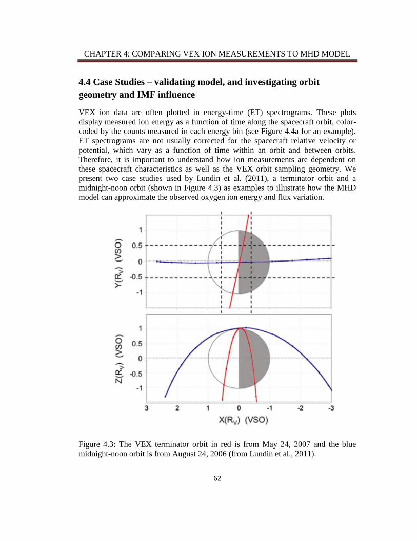
CHAPTER 4: COMPARING VEX ION MEASUREMENTS TO MHD MODEL
62
4.4 Case Studies – validating model, and investigating orbit
geometry and IMF influence
VEX ion data are often plotted in energy-time (ET) spectrograms. These plots
display measured ion energy as a function of time along the spacecraft orbit, color-
coded by the counts measured in each energy bin (see Figure 4.4a for an example).
ET spectrograms are not usually corrected for the spacecraft relative velocity or
potential, which vary as a function of time within an orbit and between orbits.
Therefore, it is important to understand how ion measurements are dependent on
these spacecraft characteristics as well as the VEX orbit sampling geometry. We
present two case studies used by Lundin et al. (2011), a terminator orbit and a
midnight-noon orbit (shown in Figure 4.3) as examples to illustrate how the MHD
model can approximate the observed oxygen ion energy and flux variation.
Figure 4.3: The VEX terminator orbit in red is from May 24, 2007 and the blue
midnight-noon orbit is from August 24, 2006 (from Lundin et al., 2011).
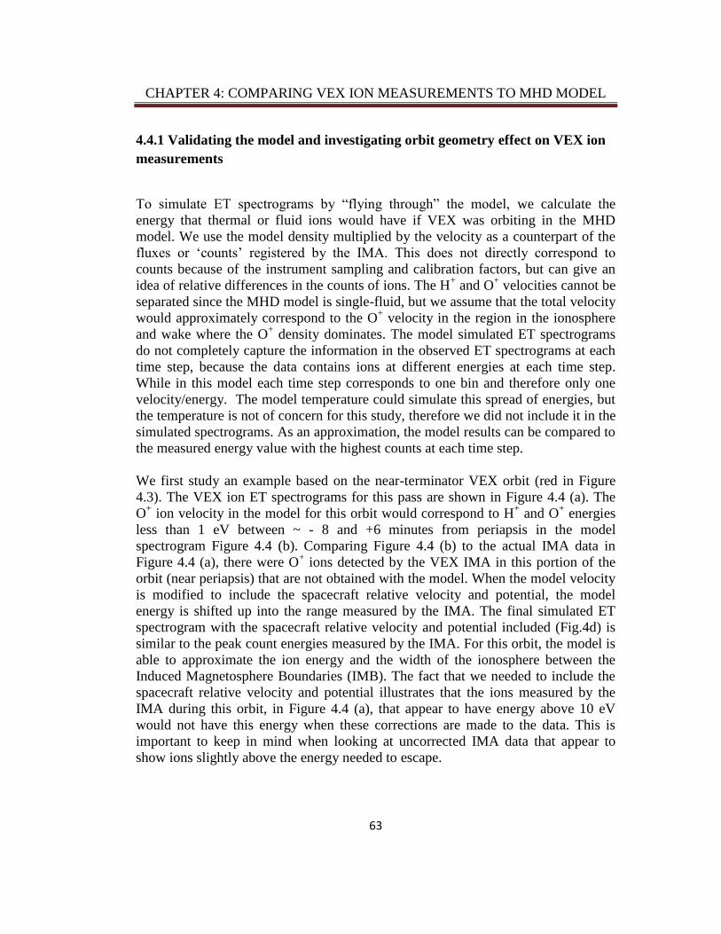
CHAPTER 4: COMPARING VEX ION MEASUREMENTS TO MHD MODEL
63
4.4.1 Validating the model and investigating orbit geometry effect on VEX ion
measurements
To simulate ET spectrograms by “flying through” the model, we calculate the
energy that thermal or fluid ions would have if VEX was orbiting in the MHD
model. We use the model density multiplied by the velocity as a counterpart of the
fluxes or ‘counts’ registered by the IMA. This does not directly correspond to
counts because of the instrument sampling and calibration factors, but can give an
idea of relative differences in the counts of ions. The H+ and O
+ velocities cannot be
separated since the MHD model is single-fluid, but we assume that the total velocity
would approximately correspond to the O+ velocity in the region in the ionosphere
and wake where the O+ density dominates. The model simulated ET spectrograms
do not completely capture the information in the observed ET spectrograms at each
time step, because the data contains ions at different energies at each time step.
While in this model each time step corresponds to one bin and therefore only one
velocity/energy. The model temperature could simulate this spread of energies, but
the temperature is not of concern for this study, therefore we did not include it in the
simulated spectrograms. As an approximation, the model results can be compared to
the measured energy value with the highest counts at each time step.
We first study an example based on the near-terminator VEX orbit (red in Figure
4.3). The VEX ion ET spectrograms for this pass are shown in Figure 4.4 (a). The
O+ ion velocity in the model for this orbit would correspond to H
+ and O
+ energies
less than 1 eV between ~ - 8 and +6 minutes from periapsis in the model
spectrogram Figure 4.4 (b). Comparing Figure 4.4 (b) to the actual IMA data in
Figure 4.4 (a), there were O+ ions detected by the VEX IMA in this portion of the
orbit (near periapsis) that are not obtained with the model. When the model velocity
is modified to include the spacecraft relative velocity and potential, the model
energy is shifted up into the range measured by the IMA. The final simulated ET
spectrogram with the spacecraft relative velocity and potential included (Fig.4d) is
similar to the peak count energies measured by the IMA. For this orbit, the model is
able to approximate the ion energy and the width of the ionosphere between the
Induced Magnetosphere Boundaries (IMB). The fact that we needed to include the
spacecraft relative velocity and potential illustrates that the ions measured by the
IMA during this orbit, in Figure 4.4 (a), that appear to have energy above 10 eV
would not have this energy when these corrections are made to the data. This is
important to keep in mind when looking at uncorrected IMA data that appear to
show ions slightly above the energy needed to escape.

CHAPTER 4: COMPARING VEX ION MEASUREMENTS TO MHD MODEL
64
Figure 4.4: (a) VEX IMA energy-time spectrograms for H+ and O
+ from May 24,
2007 - a terminator orbit. IMB = Induced Magnetosphere boundary, P = periapsis,
BS = bow shock. (b) Simulated H+ and O
+ spectrograms with energy calculated
from the MHD single-fluid velocity, color-coded by model density*velocity. (c)
Simulated O+ spectrogram from the MHD model modifying the model velocity with
the spacecraft relative velocity. (d) Simulated O+ spectrogram from the MHD model
including the spacecraft potential in addition to the spacecraft relative velocity.
In contrast to the terminator orbit where O+ was only detected by the VEX IMA
within ~ - 8 and +6 minutes from periapsis, the instrument detected O+ for nearly 50
minutes before periapsis for the midnight-noon orbit in Figure 4.5 (a). These ion
detections by the IMA included O+ with energies between 10 eV and 1 keV near
periapsis in the ionosphere and in the wake behind the planet. The MHD model is
c) MHD O+ energy
(eV) Including
spacecraft relative
velocity
d) MHD O+
energy (eV)
Including spacecraft
relative velocity and
potential
-40 -30 -20 -10 0 10 20 30 40
10
100
1000
10,000
O+
ene
rgy(
eV
)
0
2
4
10
100
1000
10,000
O+
ene
rgy(
eV
)
0
2
4
10
100
1000
10,000
O+
ener
gy(e
V)
0
2
4
log
(n*v) n in /cc v in km/sec
Time (minutes from periapsis)
10
100
1000
10,000
H+
en
erg
y(e
V)
b) MHD
H+ energy (eV)
O+ energy (eV)
a) VEX IMA
H+
O+
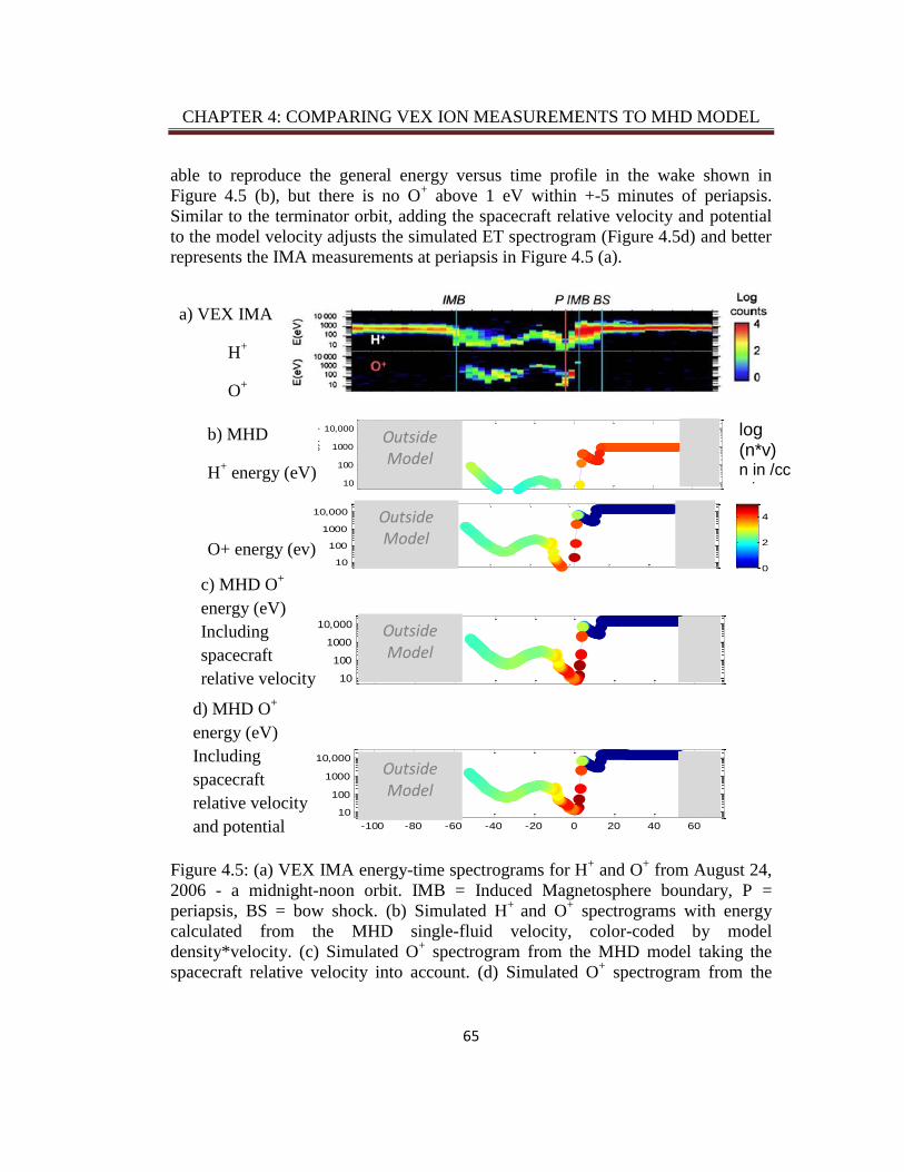
CHAPTER 4: COMPARING VEX ION MEASUREMENTS TO MHD MODEL
65
able to reproduce the general energy versus time profile in the wake shown in
Figure 4.5 (b), but there is no O+ above 1 eV within +-5 minutes of periapsis.
Similar to the terminator orbit, adding the spacecraft relative velocity and potential
to the model velocity adjusts the simulated ET spectrogram (Figure 4.5d) and better
represents the IMA measurements at periapsis in Figure 4.5 (a).
Figure 4.5: (a) VEX IMA energy-time spectrograms for H+ and O
+ from August 24,
2006 - a midnight-noon orbit. IMB = Induced Magnetosphere boundary, P =
periapsis, BS = bow shock. (b) Simulated H+
and O+ spectrograms with energy
calculated from the MHD single-fluid velocity, color-coded by model
density*velocity. (c) Simulated O+ spectrogram from the MHD model taking the
spacecraft relative velocity into account. (d) Simulated O+ spectrogram from the
c) MHD O+
energy (eV)
Including
spacecraft
relative velocity
10
100
1000
10,000
O+
ener
gy(e
V)
0
2
4Outside Model
10
100
1000
10,000
H+
en
erg
y(e
V)
Outside Model
10
100
1000
10,000
O+
ene
rgy(
eV
)
0
2
4Outside Model
-100 -80 -60 -40 -20 0 20 40 60
10
100
1000
10,000
O+
ener
gy(e
V)
time(minutes from periapsis)
0
2
4Outside Model
d) MHD O+
energy (eV)
Including
spacecraft
relative velocity
and potential
a) VEX IMA
H+
O+
log
(n*v) n in /cc v in km/sec
b) MHD
H+ energy (eV)
O+ energy (ev)

CHAPTER 4: COMPARING VEX ION MEASUREMENTS TO MHD MODEL
66
MHD model including the spacecraft potential correction in addition to the
spacecraft relative velocity.
4.4.2 IMF direction effect on ion energy-time spectrograms
VEX IMA ET spectrograms have varying shapes, even in cases with similar orbit
geometry. Dissimilar IMF direction is one possible explanation for the change in ET
spectrogram shape when the orbit geometry is similar. In order to illustrate how the
IMF direction might affect the shape of ET spectrograms, we rotated the orbits
presented in section 4.1 by angles between 0° and 315° (see Figs 6a and 7a) within
the YZ plane. We then created simulated spectrograms from the new positions
within the model. This approximates a change in the IMF clock angle.
There were slight variations in the shape of the simulated spectrograms depending
on rotation of the orbit as shown by the varying panels in Figures 4.6 (b) and 4.7 (b),
which are labeled with the angle rotation of the orbit. Corresponding magnetic field
from the model is plotted in Figures 4.6 (c) and 4.7 (c) to show which rotated orbits
pass through the magnetic draping pole (where Bx changes sign inbound versus
outbound). For the terminator orbit (Figure 4.6c) this Bx rotation appears in the
magnetic field time series of the 0° orbit (not rotated, with periapsis passing through
the northern draping pole) and the orbit rotated 180° (periapsis passing through the
southern draping pole). The spectrograms for the terminator orbit show only modest
variations in appearance for all IMF rotation angles, while the magnetic fields show
considerable change.
The actual IMF vector most often has a low Bz component, which would correspond
to a rotation of the orbit of 0° or 180° (since the model has the IMF in the XY
plane). However, the different simulated ET spectrogram shapes show that a
rotation of the IMF may change what regions (in a VSE frame) the VEX spacecraft
samples, and therefore the shape of the ET spectrogram. This is helpful for
investigators to keep in mind when comparing IMA data between different VEX
orbits because the IMF can rotate to large inclinations (especially during solar wind
disturbances). The model’s ability to simulate the general shape of the VEX IMA
ET spectrograms in the ionosphere and in the wake, for the individual VEX passes
presented in section 4.1, provides confidence it can be applied to a more global
context.
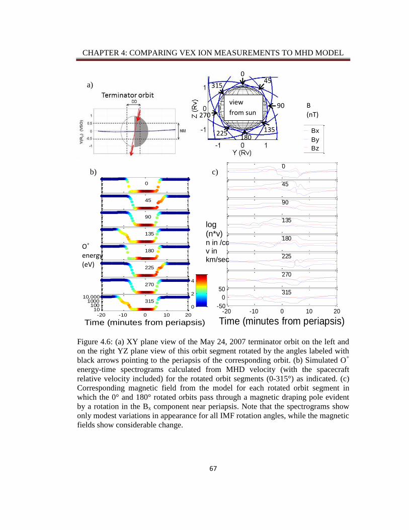
CHAPTER 4: COMPARING VEX ION MEASUREMENTS TO MHD MODEL
67
0
45
90
135
180
225
270
-20 -10 0 10 2010
1001000
10,000315
Time (minutes from periapsis)
0
2
4
0
45
90
135
180
225
270
-20 -10 0 10 20-50
0
50315
Time (minutes from periapsis)
Figure 4.6: (a) XY plane view of the May 24, 2007 terminator orbit on the left and
on the right YZ plane view of this orbit segment rotated by the angles labeled with
black arrows pointing to the periapsis of the corresponding orbit. (b) Simulated O+
energy-time spectrograms calculated from MHD velocity (with the spacecraft
relative velocity included) for the rotated orbit segments (0-315°) as indicated. (c)
Corresponding magnetic field from the model for each rotated orbit segment in
which the 0° and 180° rotated orbits pass through a magnetic draping pole evident
by a rotation in the Bx component near periapsis. Note that the spectrograms show
only modest variations in appearance for all IMF rotation angles, while the magnetic
fields show considerable change.
O+ energy (eV)
B (nT)
0
45
90
135
180
225
270
-40 -20 0 20-50
0
50315
Time (minutes from periapsis)
Bx
By
Bz
b)
a)
c)
log
(n*v) n in /cc v in km/sec
view
from sun
0 45
90
135
6 180
6
225
6
270
6
315
6
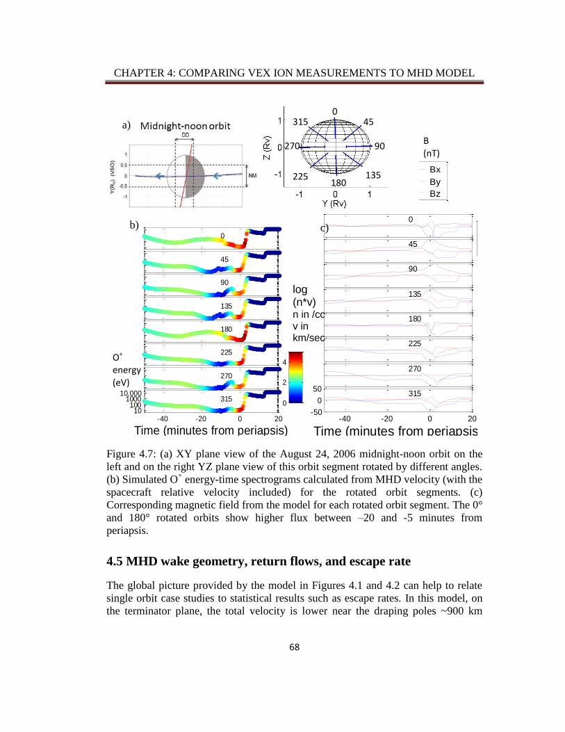
CHAPTER 4: COMPARING VEX ION MEASUREMENTS TO MHD MODEL
68
0
45
90
135
180
225
270
-40 -20 0 2010
1001000
10,000315
Time (minutes from periapsis)
0
2
4
0
45
90
135
180
225
270
-40 -20 0 20-50
0
50315
Time (minutes from periapsis)
Bx
By
Bz
Figure 4.7: (a) XY plane view of the August 24, 2006 midnight-noon orbit on the
left and on the right YZ plane view of this orbit segment rotated by different angles.
(b) Simulated O+ energy-time spectrograms calculated from MHD velocity (with the
spacecraft relative velocity included) for the rotated orbit segments. (c)
Corresponding magnetic field from the model for each rotated orbit segment. The 0°
and 180° rotated orbits show higher flux between –20 and -5 minutes from
periapsis.
4.5 MHD wake geometry, return flows, and escape rate
The global picture provided by the model in Figures 4.1 and 4.2 can help to relate
single orbit case studies to statistical results such as escape rates. In this model, on
the terminator plane, the total velocity is lower near the draping poles ~900 km
B (nT)
O+ energy (eV)
0
45
90
135
180
225
270
-40 -20 0 20-50
0
50315
Time (minutes from periapsis)
Bx
By
Bz
b)
a)
c)
log
(n*v) n in /cc v in km/sec
0 45
90
135
6 180
6
225
6
270
6
315
6

CHAPTER 4: COMPARING VEX ION MEASUREMENTS TO MHD MODEL
69
altitude, but the O+ density is higher there. This is shown in the altitude versus clock
angle contour plots in Figure 4.1 (b) and (d). Here the clock angle refers to the angle
in the YZ plane where 90° is at the magnetic draping poles (+ and –Z), see Fig 1 (a).
The H+ density in Fig 1 (c) indicates that the O
+ density in Fig 1 (d) dominates at
altitudes below ~500 km near the equator and up to altitudes of ~900 km at the
draping poles. The vectors, discussed later, are normalized flow vectors in this
plane, which are the same for all species in this model.
Comparisons to model behavior in a meridian plane (Figure 4.2a) bring out the
significant differences in the 3D model behaviors at different locations. In the model
wake, along the noon-midnight plane the high O+ density from the ionosphere
extends to higher altitudes (Figure 4.2d). Here altitude versus Solar Zenith Angle
(SZA) is used - where 0° is subsolar and 180° is in the wake. Again the arrows show
the geometry of ion flow along this plane. The model O+ density dominates the H
+
in the wake (Figure 4.2c versus Figure 4.2d).
The simulated spectrograms that we presented as case studies looked different
because of how they were sampling the 3D space of the model. The example
terminator orbit dipped into the ionosphere down to ~300 km, but the high O+
densities only occur from below ~400 km at the equator to ~900 km at the draping
poles. Therefore, the VEX orbit would not spend much time (only ~ 10 minutes)
sampling these ions in the model. The slight differences in the simulated rotated
terminator orbit spectrograms were due to different sampling of the draping poles
versus the magnetic equator. In contrast to the terminator orbit, the midnight-noon
example VEX orbit spent ~50 minutes in the wake, where the model has O+ ions
with density ~100/cc flowing to high altitudes. These showed up in the simulated
spectrograms as an extended higher density portion in the orbit. The shape of the
energy time series in the model wake is due to the asymmetric flow of ions. Higher
density ions flow into the wake from the draping poles gaining velocity as they
move into the wake, while at the equator there is lower density O+ flowing that does
not have these high velocities. We attempted to determine if draping pole
asymmetries are evident in VEX IMA data, but because the VEX orbit primarily
samples the draping poles, there were not enough non-draping pole samples (e.g.
from occasional high inclination IMF cases) for adequate comparison. In addition,
as shown by the simulated spectrograms rotated by IMF angle in the YZ plane
(Figures 4.6b and 4.7b), the asymmetry seen in the global model would not be
obvious in ET spectrograms.
4.5.1 Return Ion Flows in the Model Wake
Since Lundin et al. (2011) analyzed IMA data and found oxygen ions gravitationally

CHAPTER 4: COMPARING VEX ION MEASUREMENTS TO MHD MODEL
70
Since Lundin et al. (2011) analyzed IMA data and found oxygen ions gravitationally
bound at large distances, we explored return flows in the model. Sunward return ion
flows are not apparent in the simulated energy-time spectrograms, because the
spectrogram energy is calculated using the total velocity (i.e., the direction is not
considered). Depending on the orbit and the IMF direction, the energy-time
spectrogram may contain return flows. An example of VEX observations with
possible return flows (from June 6, 2009) is shown in Figure 4.8 by the +X O+
velocity from ~1:25 to 2:05. The return flows are confirmed by looking at the
direction that the ion detections came from (Figure 4.10), which is a plot of the
Azimuth and Polar angles where (0,0) corresponds to tailward flow. The simulated
ET spectrogram from flying this VEX orbit through the model also contains return
ion flow marked by the shaded blue area in Figure 4.9.
Figure 4.8: VEX energy time spectrogram from June 6, 2009 on the top, with
calculated O+ density, velocity components, and total velocity below. The color
code on the VEX density denotes the quality of the moments.
VEX IMA O+ E/q, eV
VEX IMA O+ density (/cc)
VEX IMA O+ velocity components (km/sec)
VEX IMA O+ total velocity (km/sec)
Vx Vy Vz
moment quality Poor Satisfactory Good Excellent
color code is log (counts)

CHAPTER 4: COMPARING VEX ION MEASUREMENTS TO MHD MODEL
71
Figure 4.9: Model simulated O+ spectrogram, O
+ density, velocity components
(solid lines include the spacecraft relative velocity and dashed lines are just ion
velocity) and total velocity (including spacecraft velocity). Blue shaded area on
simulated time series plots bounds the ~15 minute period within the VEX orbit
where return flows are sampled in the model. Both the model and the data show
sunward (+X) flowing ions in the wake, but these sunward flows in the data are
even further back in the wake than in the model.

CHAPTER 4: COMPARING VEX ION MEASUREMENTS TO MHD MODEL
72
Figure 4.10: Ion detections plotted in Azimuth and Polar angle, where (0,0)
corresponds to tailward flow. For this case, the ions are flowing sunward.
The model has ion flows turning back toward the planet in the wake as far out as
~3000 km (an X of - 1.5 Rv), as shown by yellow, orange and red shades
representing sunward O+ fluxes in Figure 4.11, where contours of model O
+ flux in
two planes (XY-the equator and XZ-the meridian plane) are displayed. These return
ion flows start near the terminator, and occur throughout a large portion of the
equator (XY plane). The ions that eventually do escape into the wake originate from
the draping poles (shown in blue at 90 degrees SZA in Figure 4.11b). These
returning flowing ions, which occur out to -1.5 Rv in the X direction in the model,
are shown in YZ plane cuts in the tail to illustrate how they affect the escape spatial
distribution in Figure 4.12. Similar to Figure 4.11, the yellow and red portions of the
figure correspond to ions turning back toward the planet. The extent to which
observations support this picture of extensive return flows seen in the model has
potential implications for global ion escape.
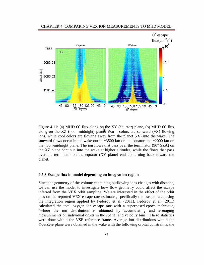
CHAPTER 4: COMPARING VEX ION MEASUREMENTS TO MHD MODEL
73
Figure 4.11: (a) MHD O+ flux along on the XY (equator) plane, (b) MHD O
+ flux
along on the XZ (noon-midnight) plane. Warm colors are sunward (+X) flowing
ions, while cool colors are flowing away from the planet (-X) into the wake. The
sunward flows occur in the wake out to ~3500 km on the equator and ~2000 km on
the noon-midnight plane. The ion flows that pass over the terminator (90° SZA) on
the XZ plane continue into the wake at higher altitudes, while the flows that pass
over the terminator on the equator (XY plane) end up turning back toward the
planet.
4.5.3 Escape flux in model depending on integration region
Since the geometry of the volume containing outflowing ions changes with distance,
we can use the model to investigate how flow geometry could affect the escape
inferred from the VEX orbit sampling. We are interested in the effect of the orbit
bias on the reported VEX escape rate estimates, specifically the escape rates using
the integration region applied by Fedorov et al. (2011). Fedorov et al. (2011)
calculated the total oxygen ion escape rate with a superposed-epoch technique,
“where the ion distribution is obtained by accumulating and averaging
measurements on individual orbits in the spatial and velocity bins”. These statistics
were done within the VSE reference frame. Average ion distributions within the
YVSEZVSE plane were obtained in the wake with the following orbital constraints: the
O+ escape
flux(cm-2
s-1
)
b)
a)

CHAPTER 4: COMPARING VEX ION MEASUREMENTS TO MHD MODEL
74
spacecraft had to be further away from the center of the planet than 1.2 Venus radii
(Rv), the XVSE was between -0.8 to -3 Rv.
Figure 4.12: O
+ escape flux (cm
-2s
-1) on YZ planar cuts in the tail at X values in the
wake of (a) -1.1 Rv, (b) -1.3 Rv, (c) -1.5 Rv, (d) -2.0 Rv.Yellow-red shades
correspond to ion flows headed back toward the planet. The pattern of escaping ions
changes with distance from the planet in the model.
Figures 4.13 (a) and (b) show the escape flux calculated from the model if the
integration region was started from different X positions behind the terminator (-0.8
and -1.6 RV). Planet-ward (return) ion flows were not included. Because the orbit
passes over the northern pole, these figures show a high flux at near Z = +1 Rv for X
= -0.8 Rv. If the integration region is started at -1.6 XVSE the orbit is no longer
sampling the region near the northern pole at altitudes where there are high ion
fluxes. A similar plot is shown for the escape flux through an YZ plane at -2 Rv
O+ escape flux(cm
-2s
-1)
b) Plane at
X=-1.3 Rv
a) Plane at
X=-1.1 Rv
d) Plane at
X=-2.0 Rv
c) Plane at
X=-1.5 Rv

CHAPTER 4: COMPARING VEX ION MEASUREMENTS TO MHD MODEL
75
XVSE in Figure 4.13 (d). By this distance into the wake, there are no longer return
flows. Therefore, all of the flow is escaping and represents the total escape through
the wake in the model.
-2 0 2-2
-1
0
1
2
Y
Z
0
1
2
3
4
5x 10
7
-2 0 2-2
-1
0
1
2
Y
Z
0
1
2
3
4
5x 10
7
Figure 4.13: Plots of the escape flux (cm-2
s-1
) calculated using the VEX orbit
starting at difference distances in the wake (a) -0.8 Rv and (b) -1.6 Rv - only
including ions flowing in the -X direction. White areas are due to no orbit sampling.
(c) XZ view of the orbits used to calculate the average escape flux in (a). (d) Escape
flux on a YZ plane at X = -2 Rv (not averaging along the X direction).
b) a)
O+ escape
flux(cm-2
s-1
)
c)
Z (Rv)
X (Rv)
d)
starting escape integration
at X=-0.8 Rv starting escape integration
at X=-1.6 Rv
side view of orbits used to
build up average in (a) d)
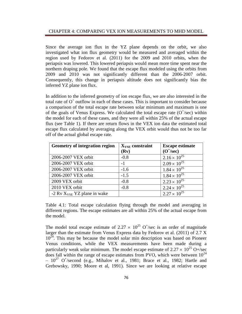
CHAPTER 4: COMPARING VEX ION MEASUREMENTS TO MHD MODEL
76
Since the average ion flux in the YZ plane depends on the orbit, we also
investigated what ion flux geometry would be measured and averaged within the
region used by Fedorov et al. (2011) for the 2009 and 2010 orbits, when the
periapsis was lowered. This lowered periapsis would mean more time spent near the
northern draping pole. We found that the escape flux modeled using the orbits from
2009 and 2010 was not significantly different than the 2006-2007 orbit.
Consequently, this change in periapsis altitude does not significantly bias the
inferred YZ plane ion flux.
In addition to the inferred geometry of ion escape flux, we are also interested in the
total rate of O+ outflow in each of these cases. This is important to consider because
a comparison of the total escape rate between solar minimum and maximum is one
of the goals of Venus Express. We calculated the total escape rate (O+/sec) within
the model for each of these cases, and they were all within 25% of the actual escape
flux (see Table 1). If there are return flows in the VEX ion data the estimated total
escape flux calculated by averaging along the VEX orbit would thus not be too far
off of the actual global escape rate.
Geometry of integration region XVSE constraint
(Rv)
Escape estimate
(O+/sec)
2006-2007 VEX orbit -0.8 2.16 1025
2006-2007 VEX orbit -1 2.09 1025
2006-2007 VEX orbit -1.6 1.84 1025
2006-2007 VEX orbit -1.5 1.84 1025
2009 VEX orbit -0.8 2.23 1025
2010 VEX orbit -0.8 2.24 1025
-2 Rv XVSE YZ plane in wake 2.27 1025
Table 4.1: Total escape calculation flying through the model and averaging in
different regions. The escape estimates are all within 25% of the actual escape from
the model.
The model total escape estimate of 2.27 1025
O+/sec is an order of magnitude
larger than the estimate from Venus Express data by Fedorov et al. (2011) of 2.7 X
1024
. This may be because the model solar min description was based on Pioneer
Venus conditions, while the VEX measurements have been made during a
particularly weak solar minimum. The model escape estimate of 2.27 1025
O+/sec
does fall within the range of escape estimates from PVO, which were between 1024
– 1027
O+/second (e.g., Mihalov et al., 1981; Brace et al., 1982; Hartle and
Grebowsky, 1990; Moore et al, 1991). Since we are looking at relative escape

CHAPTER 4: COMPARING VEX ION MEASUREMENTS TO MHD MODEL
77
estimates in the model, the uncertainty in the accuracy of the total escape rate in the
model does not affect our conclusions.
4.6 Conclusions
Low energy ion measurements are complicated by the spacecraft’s relative velocity
and potential. These spacecraft characteristics can upshift ion energies in the data to
make ions seem to have enough energy to escape from the planet, when in reality
they may not. Orbit geometry and IMF direction can also affect the shape of energy-
time spectrograms. When undertaking case studies of Venus Express orbits it is
important to consider that the time series of ion energies are generally not corrected
for the spacecraft’s relative velocity or potential, and that the orbit geometry and
IMF direction must be considered on a case-by-case basis. We were able to
reproduce the general shape of VEX ion energy-time spectrograms at low energies
(< 1 keV) in the ionosphere and wake using an MHD model.
We also considered the consequences for escape of both these energy corrections
and the VEX orbit sampling. The inferred escape flux spatial distribution averaged
in the YZ plane in the model along the VEX orbit looked different depending on the
region in the wake used to integrate the measurements. The MHD model has ion
flows turning back toward the planet out to -1.5 Rv in the wake, and Lundin et al.
(2011) suggested that extended return flows may also exist in the VEX IMA data.
These return flows can change that total escape flux inferred by averaging along the
VEX orbit, but only by ~20%, thus these are not a major concern considering the
other sources of error in the measurements. Nevertheless, it is important for users of
low energy ion measurements to use caution in interpreting such observations.
Indeed, the errors can be a major source of differences obtained in different studies.
Separating such measurement complications from natural variations is a particular
challenge, and should moderate arguments regarding accuracy of these fluxes.
Perhaps reported results should be viewed as order of magnitude in accuracy at best
with only exceptional changes meriting debate.
78
Chapter 5
Effects of a Large ICME on Oxygen Ion Escape at Venus
Abstract
Understanding the effects of large solar wind disturbances on O+ ion escape is
critical for characterizing the history of water on Venus. Previous studies suggested
that disturbances can enhance the ion escape rate, but did not specifically study how
escape is affected during the passage of the sheath region of a fast interplanetary
coronal mass ejection (ICME). During ICME sheaths, the highest dynamic pressures
in the solar wind occur. We present a case study of a large ICME that impacted
Venus on November 5, 2011, and had the highest magnetic field yet encountered by
Venus Express (VEX) (>250 nT). This event is unique because VEX was near
Venus right at the time the ICME sheath was present. This is a circumstance that has
occurred only a small fraction of the time VEX has been sampling ions near its
periapsis. Oxygen ion escape was enhanced during this event compared to the days
before and after the event when no ions were observed escaping into the wake
5.1 Introduction
Quantifying the present oxygen ion escape rate and its variation with external
conditions is crucial to reconstructing the history of water on Venus (in addition to
measurements of isotope ratios, estimates of the past solar activity, and escape
models) as discussed by Chassefiere et al. (2012). Ion escape rates were estimated
using instruments on Pioneer Venus Orbiter (PVO) (e.g., Brace et al., 1995), but
none of these instruments were capable of fully characterizing the ion escape by
species and at all energies expected for escaping ions. Venus Express (VEX) has an
ion instrument, the ASPERA-4 (Analyzer of Space Plasmas and Energetic Atoms)
CHAPTER 5: INFLUENCE OF A LARGE ICME ON ION ESCAPE AT VENUS
79
Ion Mass Analyzer (IMA) detailed in Barabash et al. (2007a), that can determine the
composition of the escaping species over a broad energy range ~10eV-25keV.
However, VEX launched just prior to the recent solar minimum. As a result, VEX
ASPERA-4 ion escape statistics have only been published for low solar activity
conditions when the largest variations in solar wind conditions, caused by major
ICMEs, are generally absent (Barabash et al., 2007b and Fedorov et al., 2011).
Hence, previous studies suggesting that O+ escape may be enhanced at disturbed
times (Luhmann et al, 2007; Futaana et al., 2008; Luhmann et al., 2008; Edberg et
al., 2011) could not be verified. In addition, Luhmann et al. (2008) found that in
three out of four case studies of moderately disturbed conditions in the earlier part
of the mission, ICME passage did not produce apparent enhancements in the
inferred ion escape. McEnulty et al. (2010) similarly did not find an increase in the
escape flux during ICMEs, specifically at the highest-energies. The question has
then been left open as to whether there is indeed a ‘space weather’ effect on Venus
ion escape and if so, is solar wind dynamic pressure the main factor in its
importance?
The highest dynamic pressures in the solar wind are within large ICMEs. As an
ICME propagates away from the Sun it interacts with the background undisturbed
solar wind. At the leading edge of the ICME, the interplanetary magnetic field
(IMF) and solar wind is compressed (see Figure 5.1). This compression results in
high total magnetic field and high dynamic pressure and is called the ICME sheath.
This compressed sheath region lasts for a few hours (as measured at Venus). The
main body (ejecta) of the ICME then follows the sheath region. This ejecta portion
is often associated with a magnetic cloud, which has a rotating IMF and is smoother
(less variance) than the sheath region. This magnetic cloud signature can last for 1-4
days at Venus. (For more details of ICME time series see Jian et al., 2006, 2008).
Since the earlier studies were published, solar activity has increased and ICMEs
observed in the solar wind near Venus have become faster and larger, with
associated greater solar wind plasma and field modifications. In the present study,
we look closely at escape during the highest dynamic pressures seen in the solar
wind so far on VEX – in the sheath region of a large ICME. The average dynamic
pressure during the VEX mission from 2006-2009 was 1.5 nPa (McEnulty et al.,
2012a) and the dynamic pressures in the study of Edberg et al. (2011) did not
exceed 4 nPa. However, the dynamic pressure in the ICME sheath region at Venus,

CHAPTER 5: INFLUENCE OF A LARGE ICME ON ION ESCAPE AT VENUS
80
based on PVO statistics which spanned a solar cycle, can often exceed 20 nPa even
reaching 80 nPa (e.g., Jian et al., 2006, 2008; McEnulty et al, 2012a). When the
dynamic pressure is high, the altitude of the boundary between the Venus
ionosphere and the solar wind (the ionopause) is lowered (e.g., Phillips et al, 1985).
A lower ionopause altitude can expose more ionospheric particles to the solar wind
convection electric field, possibly enhancing their escape (Luhmann et al., 2006).
Figure 5.1: Cartoon of an ICME propagating into the ambient solar wind. Fast
ICMEs compress the solar wind in front of them causing a region of high density
and dynamic pressure. (from J. Luhmann, personal comm.)
In order to measure the ion escape during the time of most interest, the spacecraft
must be near the planet when the ICME sheath passes. This does not occur often
because VEX has a 24 hour orbital period, and is only near the planet measuring ion
escape for ~2 hours of the orbit. The typical fast ICME passes an observer at Venus’
heliocentric distance in ~a day, but the ICME sheath passage only lasts for a few
hours. Thus most ICME sheaths pass the planet when VEX is away from its
periapsis and not measuring planetary ions. There was fortunate timing on
November 5, 2011, when a large (fast and high magnetic field) ICME hit Venus just
as the spacecraft was nearing the planet. Figure 5.2 shows the location of Venus
together with the locations of the STEREO (Solar TErrestrial RElations
Observatory) twin spacecraft, which were observing solar activity from widespread

CHAPTER 5: INFLUENCE OF A LARGE ICME ON ION ESCAPE AT VENUS
81
multiple perspectives at this time. In this paper, we show this ICME as imaged by
STEREO A and B and the response of Venus to this event as seen on VEX in both
magnetic field and ion measurements during the ICME sheath passage. The general
properties of the VEX ASPERA-4 IMA and Magnetometer (MAG) measurements
used in this study are described in Barabash et al. (2007a) and Zhang et al. (2006),
respectively, and will not be repeated here.
Figure 5.2: Locations of Venus, STEREO A, and STEREO B on November 5, 2011.
5.2 November 3, 2011 Coronal Mass Ejection
The Coronal Mass Ejection (CME) of interest occurred at the end of the day on
November 3, 2011 on the far side of the Sun as seen from Earth. The location of the
STEREO A and B spacecraft allowed imaging of this event from multiple
viewpoints. This event produced a partial halo in the STEREO B white-light
coronagraph COR2 image shown in Figure 5.3. The COR2 detectors observe within
a region from 2-15 solar radii, as described in Howard et al. (2008). The location of
Venus and the STEREO twin spacecraft (Figure 5.2) were thus useful in
understanding both the origins and characteristics of the event that impacted the
planet. The CME speed estimated from STEREO A was 1038 km/sec
(http://spaceweather.gmu.edu/seeds/). To put this CME speed into context, the
average speed of CMEs that impacted Venus in 2006-2007 from McEnulty et al.

CHAPTER 5: INFLUENCE OF A LARGE ICME ON ION ESCAPE AT VENUS
82
(2010) was only 250 km/sec. Also, from 10 years of PVO observations, the average
speed of ICMEs was 476 km/sec. (See Table 2 of Jian et al., 2008.)
Figure 5.3: White-light coronagraph images from STEREO A (left) and B (right)
showing a partial halo toward STEREO B at the beginning of the day on November
4, 2011. This event started at the end of the day on Nov 3rd
, shown on the left
5.3 ICME at Venus
An ICME was measured in the VEX magnetic field and plasma data on November
5, 2012 03:00 UT. This ICME arrived at Venus within a few hours of the time
calculated from the speed of the Nov 3 CME discussed in the previous section.
Figure 5.4(b-e) displays the IMF near Venus measured by the Venus Express
magnetometer in VSO (Venus-solar-orbital) coordinates (where X is toward the sun,
Y is opposite the orbital direction, and Z completes the right hand system). The
sheath region lasted for ~ 6 hours, and the ejecta portion for ~18 hours. This
disturbance was also observed in the solar wind plasma. Before the ICME arrived at
Venus, the H+ measured within the solar wind by the VEX IMA had an energy of
~1.5 keV. After the ICME arrived, the solar wind H+ had energies above 10 keV,
even up to 20 keV in the ICME sheath. This increase in the background H+ energy is
illustrated with an energy-time (ET) spectrogram created from the VEX IMA data in
Figure 5.4a. This ET spectrogram is a plot of the measured H+ ion energy (at time
steps averaged every 3 minutes). The color code is log(counts) of the measured H+.

CHAPTER 5: INFLUENCE OF A LARGE ICME ON ION ESCAPE AT VENUS
83
Gaps on this plot occur during time periods when the IMA instrument is not
operating. H+ measured near Venus has energies below ~ 1 keV, which appears on
the ET spectrogram every day for ~ 2 hours as the VEX spacecraft nears the planet
in its 24 hour orbit. The solar wind dynamic pressure calculated from IMA density
and velocity (downloaded from http://cdpp-amda.cesr.fr/) for this event was 17.6
nPa (density 13/cc, velocity 900 km/sec). For comparison, before the event the
dynamic pressure was 0.72 nPa (density 3/cc, velocity 345 km/sec). The VEX
spacecraft was near periapsis and sampled planetary ions near Venus during the
ICME sheath (the Btot increase up to 260 nT, and the H+ detections on low energies
on Nov 5th
were in the green shaded region on Figure 5.4).
-50
0
50
Bx
-50
0
50
By
-50
0
50
Bz
11/05 11/06 11/07 11/080
100200300
Bto
t
Figure 5.4: (a) VEX IMA H
+ detections plotted as a function of time and energy and
color-coded for H+ log (counts). (b-d) VEX magnetic field vector components and
(e) total magnetic field strength. An ICME solar wind disturbance was detected on
November 5, 2011 in both the magnetic field and solar wind H+. The ICME sheath
H+ energy (eV)
log(counts)
for H+
shock
Increase in H+ energy
(a)
(b)
(c)
(d)
(e) Venus interaction

CHAPTER 5: INFLUENCE OF A LARGE ICME ON ION ESCAPE AT VENUS
84
is shaded in green, and the blue shaded time period is the ICME ejecta. Daily spikes
are due to the interaction of the IMF with the Venus ionosphere.
5.4 O+ detections during the ICME and comparison to an
undisturbed orbit
As the VEX spacecraft moves closer to Venus it begins to measure heavier mass
ions in addition to the solar wind H+. These ions can be detected within the
magnetosheath where the IMF piles up above the ionosphere obstacle (see Figure
5.5). This obstacle occurs at the ionopause, where the solar wind dynamic pressure
on the outside balances the thermal pressure from the ionospheric plasma on the
inside. The VEX IMA also detects O+ beneath the ionopause (in the ionosphere) and
in the wake (e.g., Barabash et al, 2007b; Fedorov et al., 2011).
Figure 5.5: Cartoon of the Venus-solar wind interaction. The dashed lines on the
left with arrows represent the flowing solar wind particles carrying with them the
interplanetary magnetic field lines (vertical and perpendicular to the flow in this
case). These field lines pile up near the ionosphere in the magnetosheath and drape
around the planet. The ionopause is the boundary between the region of solar wind
particles and the ionosphere. In this figure ions are represented by circles on the
dayside with pluses and minuses. In the wake (the region on the nightside where
there is little solar wind), the field lines that have slipped over the planet form a
magnetotail. (from Luhmann and Russell 1997)
wake
ionosphere
CHAPTER 5: INFLUENCE OF A LARGE ICME ON ION ESCAPE AT VENUS
85
We are interested in details of the O+ measured within the magnetosheath,
ionosphere, and wake of Venus when the large ICME impacted Venus. We also
want to know how the O+ behavior during the large ICME compares to O
+ measured
during undisturbed solar wind conditions. To determine the influence of ICMEs it is
important to control for other aspects that can affect the O+ measurements, such as
the orbit and IMF direction. The measured O+ will depend on the spacecraft’s orbit
due to sampling different spatial regions and is affected by the spacecraft’s relative
velocity as described in McEnulty et al. (2012b).
The most straightforward comparison is of the O+
detected on November 5, 2011 to
measurements of O+ within a few days of Nov 5, but before the ICME arrived at
Venus. The VEX orbit does not change significantly within 2 days, so we compare
to November 3, 2011. During this time period (Nov 3-5), VEX was in an orbit
moving from the sunward side to the night side, referred to as noon-midnight (see
Figure 5.6a and b). On Nov 3, O+ was detected within the magnetosheath near the
ionopause, and at low energies (<40 eV) within the ionosphere. On Nov 5, the
ionopause was at a lower altitude, and the magnetosheath was compressed (as
would be expected from high dynamic pressure in the solar wind). There was also
O+ detected in the magnetosheath near the ionopause, but it was of higher energy
and counts than on Nov 3. The O+ detected within the ionosphere and wake was of
much higher energy than on Nov 3, but not necessarily higher counts, and even
lower counts within the wake. In addition, high energy O+ was detected up to 20
keV, which was not detected on Nov 3. Comparisons of IMA O+ ions (along with
the H+ ions to show the solar wind background) periapsis are plotted in ET
spectrograms in Figure 5.7 and 5.8. These plots show the counts color-coded at each
time step (which is averaged every 3 minutes) as a function of energy. The
ionopause is marked with the white line closest to periapsis (marked with the yellow
dotted line). The color along the orbit plots of Figure 5.6a and b corresponds to the
rectangles at the bottom of the energy-time spectrograms showing where the ions
were detected within the orbits.

CHAPTER 5: INFLUENCE OF A LARGE ICME ON ION ESCAPE AT VENUS
86
-3-2-101
-1
0
1
-1
0
1
X (Rv)
Y (Rv)
Z (
Rv)
Figure 5.6: (a,b) VEX noon-midnight orbits color coded red, green, and yellow in
the regions that planetary ions were detected on Nov 3 and Nov 5, respectively.
These colored orbit segments correspond to the time periods of ion detections
marked by rectangles at the bottom of Figure 5. a and b.
Figure 5.7: VEX IMA H+ (top) and O
+ (bottom) detections plotted as a function of
time and energy and color coded for counts for November 3, 2011 (during
undisturbed solar wind). Colored rectangles at the bottom of the plots (red, green,
and yellow) correspond to the orbit segments in Figure 5.6.
solar
wind H+
H+ e
ner
gy (
eV
) 0
+ en
ergy
(eV
)
ionopause
periapsis
(b) (a)

CHAPTER 5: INFLUENCE OF A LARGE ICME ON ION ESCAPE AT VENUS
87
Figure 5.8: VEX IMA H+ (top) and O
+ (bottom) detections plotted as a function of
time and energy and color coded for counts on November 5, 2011 (when an ICME
was passing Venus). Colored rectangles at the bottom of the plots (red, green, and
yellow) correspond to the orbit segments in Figure 5.6. There was increased energy
of the H+ and O
+ ions near the planet during the ICME.
5.5 O+ escape during ICME compared to undisturbed orbits
In the previous section, we discussed O+ detections during the Nov 5 ICME
compared to detections during undisturbed solar wind conditions on Nov 3. The O+
during the ICME had higher energy, but the difference in counts (which relates to
flux) was not as clear. During the ICME, the counts were higher in the
magnetosheath and there were high energy ions (>1 keV) detected on the outbound
section of the orbit that weren’t detected on the undisturbed day. However, within
the ionosphere the counts were similar during the ICME and the undisturbed day. In
the wake (~7:30-7:40), the ICME had lower counts than the undisturbed day. In
order to understand the total difference in O+ escape flux measured during these
orbits, we must make sure that all of these ions are actually escaping. The flow
direction of O+ is a major concern when determining if the ions are actually
escaping, because O+ ions have been detected gravitationally bound and perhaps
flowing back toward the planet out to ~1.5-2 Venus Radii in the wake (Lundin et al.,
2011; McEnulty et al., 2012b). For additional comparison, we added another
example of undisturbed ion flow on November 4, 2011 to our analysis, which had
low energy detections similar to Nov 3 (see Figure 5.9. Labels and arrows on Figure
5.9 correspond to times of interest for studying detailed O+ flow direction.
solar
wind H+
H+ e
ner
gy (
eV
) 0
+ e
ner
gy (
eV)
periapsis ionopause
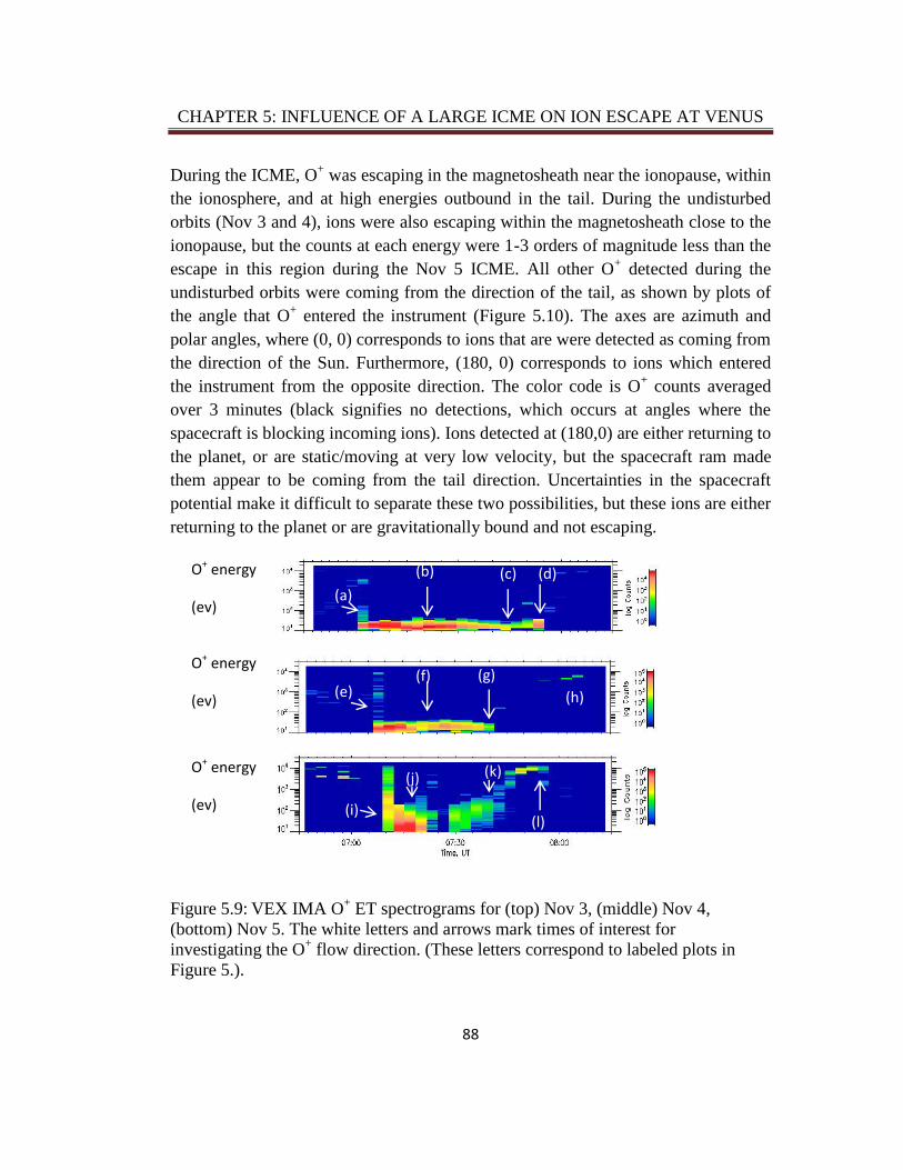
CHAPTER 5: INFLUENCE OF A LARGE ICME ON ION ESCAPE AT VENUS
88
During the ICME, O+ was escaping in the magnetosheath near the ionopause, within
the ionosphere, and at high energies outbound in the tail. During the undisturbed
orbits (Nov 3 and 4), ions were also escaping within the magnetosheath close to the
ionopause, but the counts at each energy were 1-3 orders of magnitude less than the
escape in this region during the Nov 5 ICME. All other O+ detected during the
undisturbed orbits were coming from the direction of the tail, as shown by plots of
the angle that O+ entered the instrument (Figure 5.10). The axes are azimuth and
polar angles, where (0, 0) corresponds to ions that are were detected as coming from
the direction of the Sun. Furthermore, (180, 0) corresponds to ions which entered
the instrument from the opposite direction. The color code is O+ counts averaged
over 3 minutes (black signifies no detections, which occurs at angles where the
spacecraft is blocking incoming ions). Ions detected at (180,0) are either returning to
the planet, or are static/moving at very low velocity, but the spacecraft ram made
them appear to be coming from the tail direction. Uncertainties in the spacecraft
potential make it difficult to separate these two possibilities, but these ions are either
returning to the planet or are gravitationally bound and not escaping.
Figure 5.9: VEX IMA O+ ET spectrograms for (top) Nov 3, (middle) Nov 4,
(bottom) Nov 5. The white letters and arrows mark times of interest for
investigating the O+ flow direction. (These letters correspond to labeled plots in
Figure 5.).
O+ energy
(ev)
O+ energy
(ev)
O+ energy
(ev)
(a)
(b) (c) (d)
(e) (f)
(h)
(i)
(j) (k)
(l)
(g)

CHAPTER 5: INFLUENCE OF A LARGE ICME ON ION ESCAPE AT VENUS
89
To get an approximate estimate of the O+ escape flux during the Nov 5 ICME, we
then used density and velocity moments from http://cdpp-amda.cesr.fr/. Since the O+
detected in the ionosphere and wake region was not all escaping, we focused on the
O+ detected in the dayside magnetosheath and on the outbound high energy ions in
the tail (labeled (i) and (l) on Figure 5.9). The O+ in the dayside magnetosheath had
a density of 10 O+/cc and a velocity in the –XVSO direction of 35 km/sec. This
corresponds to an escape flux of 3.5x10⁷ O
+cm
-2sec
-1. For the outbound high energy
ions, the density was 10 O+/cc and velocity in the –XVSO direction was 250 km/sec.
This corresponds to an escape flux of 2.5x10⁸ O
+cm
-2sec
-1 within this outbound
wake/magnetosheath region during the ICME.
Figure 5.10: IMA O
+ detections plotted by the angle that they are entering the
instrument (averaged over 3 minutes). In these plots, O+ detected at an azimuth and
polar angle of (0, 0) is due to ions that are coming from the sunward direction
moving tailward. (180, 0) corresponds to ions coming from the opposite direction
(moving toward the Sun). These plots correspond to the times labeled with the white
arrows and letters in Figure 5.: a) Nov 3/07:01, b) Nov 3/07:18, c) Nov 3/07:40, d)
(a)
(b)
(c)
(d)
(e)
(f)
(g)
(h)
(i)
(l)
(j)
log(counts)
O+
(k)

CHAPTER 5: INFLUENCE OF A LARGE ICME ON ION ESCAPE AT VENUS
90
Nov 3/07:50, e) Nov 4/07:07, f) Nov 4/07:18, g) Nov 4/07:40, h) Nov 4/08:02, i)
Nov 5/07:09, j) Nov 5/07:18, k) Nov 5/07:40, l) Nov 5/07:47.
In order to compare these measurements to average undisturbed conditions, we must
consider the IMF direction. Statistical studies of ion escape, such as Fedorov et al.
(2011) put the escaping ions into the VSE (Venus-Sun-Electrical) frame. In this
reference frame, ZVSE is parallel to the convection electric field, XVSE is antiparallel
to the solar wind velocity, and YVSE completes the system. From mid-2006 to 2007
the average O+ escape flux in the region between YVSE -0.5 to 0.5 and ZVSE -1.0 to
1.0 was ~5x10⁶ O
+cm
-2sec
-1, while a few spatial bins were higher than 10
7 O
+cm
-
2sec
-1 (see the left of Figure 5.11, which was from Fedorov et al., 2011). Outside of
this region, the escape flux varied between 5x10⁴ O
+cm
-2sec
-1 to
5x10
6 O
+cm
-2sec
-1.
Fedorov et al. (2011) did not include measurements made sunward of -0.8 XVSE, so
we only compare our outbound measurements, which were from the wake. This
escape flux of 2.5x10⁸ O
+cm
-2sec
-1 is higher than any of the values from Fedorov et
al. (2011). In addition, due to the IMF during this orbit, the measurements were
made away from the region of highest flux in the VSE frame described above (see
Figure 5.11). Because of this IMF affect, it is possible that the escape flux was even
higher than 2.5x10⁸ O
+cm
-2sec
-1 in the VSE locations that the spacecraft did not
sample. The only way to confirm this is to wait for more large ICMEs with diverse
VSE frame orbital sampling.
Figure 5.11: (left) Average escape flux in the VSE frame mid-2006-2007 (from
Fedorov et al., 2011). (right) Location (in the VSE frame) of O+ detections outbound
on November 5, 2011.
Econv
YVSE
ZVS
E
escape flux =
2.5x10⁸ O+cm-2sec-1

CHAPTER 5: INFLUENCE OF A LARGE ICME ON ION ESCAPE AT VENUS
91
5.6 Conclusions
An ICME impacted Venus on November 5, 2011 with timing unique for studying its
effect on escaping oxygen ions - VEX was measuring planetary ions during the high
dynamic pressure sheath region of the ICME. This timing is rare, because the high
dynamic pressure sheath region of ICMEs typically only takes a few hours to pass,
and the VEX spacecraft only measures planetary ions for a few hours out of each
24-hour orbit. This event was also unique, because it has a dynamic pressure of
17.6 nPa, which is significantly higher than the average dynamic pressure that VEX
has measured (~1.5 nPa) and of other solar wind disturbances that VEX encountered
(up to 4 nPa) (Edberg et al., 2011). In addition, the magnetic field near Venus
reached 250 nT. This is the highest field yet measured in the mission. The location
of Venus with respect to the twin STEREO spacecraft, allowed confirmation that
the ICME came from the far side of the Sun (with respect to Earth) and had a speed
of ~1000 km/sec.
During this event, on November 5, 2011, O+
coming from the atmosphere of Venus
was measured to have much higher energies than the previous 2 days (when the
solar wind was undisturbed). Detailed study revealed that in fact, the majority of the
O+ detected on the undisturbed orbits was not escaping from the planet. Instead it
was was turning back toward the planet or gravitationally bound in the wake. The
one region within the Venus-solar wind interaction that had escaping O+ on all three
days was in the dayside magnetosheath in a thin layer near the ionopause. Within
this region, the counts of escaping O+ were enhanced by up to three orders of
magnitude. O+ was also detected at high energies in the wake during the ICME with
an escape flux of 2.5x10⁸ O
+cm
-2sec
-1. Similar escaping ions were not detected
during our case studies of undisturbed orbits. Therefore, we instead compared this
flux to the average escape fluxes in the wake from Fedorov et al. (2011). This
escape flux was higher than any of the average escape fluxes. In addition, the IMF
during this ICME would have actually biased the orbital sampling to lower O+
fluxes, which makes it possible that escape fluxes were even higher in different
regions of the VSE frame that the spacecraft did not sample. However, there was
also a region in the wake that had lower counts during the ICME than during the
undisturbed days. Perhaps the gravitationally bound ions that were detected in the
wake on Nov 3 and 4 were energized to escape velocity by the ICME on Nov 5.

CHAPTER 5: INFLUENCE OF A LARGE ICME ON ION ESCAPE AT VENUS
92
Future studies can build a statistical picture in the VSE reference frame of the O+
escape flux during large ICMEs. For now, we can only speculate that the escape
flux that VEX measured during the November 5, 2011 ICME could be a lower
bound. If this were true, the lower bound on the total escape flux escaping within a
circle of radius 1 Rv during this large event would be 2.8x1026
O+/sec. For an escape
region of 1.5 Rv, the total escape would be 6.5x1027
O+/sec. This is 3 orders of
magnitude higher than the average escape rate measured by VEX of 2.7x1024
O+/sec, which highlights that ICMEs may have a significant affect on the total
escape over time. If the O+ escape is enhanced to the level suggested by this study, it
could have been even more important early in the solar system when the Sun was
likely more active (with more frequent large ICMEs). In addition, although this
ICME was the highest dynamic pressure encountered by VEX thus far (17.6 nPa), it
still is much weaker than some of the largest ICMEs that impacted Venus during
PVO (>80 nPa). As VEX continues to make measurements into solar maximum
events of this size may enhance O+ escape even further.

93
Chapter 6
Conclusion
6.1 Summary
In this dissertation, my goal was to contribute to understanding the global picture of
oxygen ion escape from Venus to space, and how escape is influenced by extreme
solar wind conditions in ICMEs. The work in this dissertation started
chronologically with the study focused on high energy O+ pick-up ions during
ICMEs (Chapter 3). This first study did not include the lower energy O+
ion
population that is also measured by VEX, because these low energy ions were
difficult to interpret. In particular, there was an open question of whether or not
these ions were even escaping. The main result of this high energy pick-up ion study
was that the O+
pick-up ions reach higher energies at lower altitudes (compared to
O+ escaping when the solar wind was undisturbed), but the O
+ counts were not
significantly affected. The result that the O+ counts were not affected raised the
following questions, which motivated the other studies in this dissertation: Is VEX
measuring O+
escape during external conditions that are representative of average
solar minimum conditions? What happens to the low energy O
+ population
during
ICMEs? Is the O+
escape rate different during large (fast) ICMEs that did not occur
during the time period of the first study?
The following three studies completed for this dissertation addressed these
questions. Comparison of the external conditions encountered by VEX to the
conditions during Pioneer Venus (Chapter 2) highlighted that VEX is measuring
CHAPTER 6: CONCLUSION
94
during a particularly weak solar minimum. Through 2009, VEX had not
encountered the high dynamic pressures that PVO had (>20 nPa), which may be
associated with enhanced ion escape. To study the low energy ion population, I
compared VEX data to an MHD model in Chapter 4. This comparison showed that
it was possible for the low energy ions measured by VEX to be gravitationally
bound and not escaping, even though they appeared to have above escape velocity
in the ion measurements. This study also pointed out that some ions measured by
VEX may be heading back toward the planet, and therefore not escaping. This result
was important to inform the last study of this dissertation, which studied O+
escape
at both low and high energies during a large ICME. The last study (Chapter 5),
revealed that O+
escape was enhanced in both the low and high energy ion
populations during a large ICME.
6.2 Major scientific contributions
I have made new and interesting discoveries in understanding the external
conditions at Venus, the geometry of oxygen ion escape, and how escape can be
affected by ICMEs. Below is a list of major contributions of the work presented in
this dissertation:
External conditions at Venus
Venus Express has been making measurements of oxygen ion escape during
a time of particularly weak solar wind dynamic pressure. In particular,
through the end of 2009 VEX had not measured any dynamic pressures
above 20 nPa, while PVO measured up to 80 nPa.
Geometry of oxygen ion escape at Venus
There are high energy (~1-30 keV) pick-up oxygen ions within the Venus
magnetosheath and during ICMEs they reach high energy at a lower altitude
(smaller gyroradius) than at undisturbed times.
Low energy (<100 eV) oxygen ions measured by VEX within the ionosphere
and in the wake must be investigated in detail before interpretation. The
measured energy of the O+
is affected by the spacecraft relative velocity and
potential. These effects can make gravitationally bound ions appear to be
moving above escape velocity.
CHAPTER 6: CONCLUSION
95
Besides being gravitationally bound, some low energy ions measured by
VEX in the wake are actually moving back toward the planet. Similar
“return flows” are also seen in an MHD model.
An MHD model is able to approximate the ion energies in the wake and is
useful for putting case studies within a global picture.
Influence of ICMEs on oxygen escape from Venus
ICMEs can accelerate high energy pick-up ions to higher energies at low
altitudes, compared to undisturbed days. However, for the ICMEs in 2006-
2007 with average velocity ~250 km/sec there was no change in the escape
rate.
Large (fast) ICMEs, with high dynamic pressure can enhance the oxygen
escape rate.
6.3 Implications for future Venus ion escape studies
The statistics of the solar wind and IMF conditions that can affect ion escape (in
Chapter 2) can be used to guide future comparisons of different time periods. I
learned that the conditions that VEX has encountered are much less intense than
what is possible. This should be kept in mind in interpreting the absolute escape
rates that are measured by VEX, even at solar maximum (since this maximum may
be weak).
The work comparing VEX data to an MHD model (Chapter 4) can be used in
interpreting future total escape rate estimates. Investigators that work with VEX ion
data should be aware of the return ion flows in case studies, such as my large ICME
study. Without an awareness of the possibility of return flow, I may have
misinterpreted the difference in ion escape during this ICME. In addition, this paper
pointed out the importance of considering the spacecraft’s relative velocity when
studying ions near periapsis. Ions can appear to have above escape velocity even
though they are actually gravitationally bound.
The results from the large ICME study (Chapter 5) highlight that the sheath of the
ICME is of particular interest for future statistical studies. Instead of considering
escape during the few days that the ICME lasts and then averaging the escape rate

CHAPTER 6: CONCLUSION
96
over that time period, future studies should separate the effects of the sheath and
ejecta portion.
6.4 Future work
Mars does not have a dynamo magnetic field, so its upper atmosphere interacts with
the solar wind similar way to Venus. I plan to use what I have learned about Venus,
and conduct similar studies at Mars on the effects of extreme solar wind on ion
escape. An interesting difference between Mars and Venus is that Mars has remnant
crustal magnetic fields. I am curious how the crustal magnetic fields change the ion
escape processes. I would like to study what happens to the atmosphere and ion
escape when there is magnetic reconnection between the crustal fields and the
interplanetary magnetic fields. The Mars Express (MEX) spacecraft carries a sister
instrument to the VEX IMA that produces similar ion data. MEX does not have a
magnetometer, making it significantly more difficult to interpret the ion data. There
was a period of overlap in the operation of MEX and the Mars Global Survey
(MGS) mission, and MGS did have a magnetometer. It would be interesting to
identify signatures of magnetic reconnection the MGS magnetometer data and then
investigate if there was anything unusual in the MEX IMA data at those times.
Mars atmospheric escape science will become even more exciting within the next
few years. A mission called MAVEN (Mars Atmosphere and Volatile EvolutioN)
will be launched in late 2013. The main goal of this mission is to understand the
history of volatiles on the planet, and part of the puzzle is to quantify ion escape
rates and their dependence on extreme solar wind conditions. MAVEN will have
multiple plasma instruments that will cover the full energy range that we expect for
O+ escape, and will have a magnetometer.

97
Bibliography
Barabash, S. et al. (2006), The Analyzer of Space Plasmas and Energetic Atoms
(ASPERA-3) for the Mars Express Mission, Space Science Reviews, 126,
113–164, doi:10.1007/s11214-006-9124-8.
Barabash, S. et al. (2007a), The Analyser of Space Plasmas and Energetic Atoms
(ASPERA-4) for the Venus Express mission, Planetary and Space Science,
55, 1772–1792, doi:10.1016/j.pss.2007.01.014.
Barabash, S. et al. (2007b), The loss of ions from Venus through the plasma wake,
Nature, 450, 650–653, doi:10.1038/nature06434.
Bauer, S. J., and H. A. Taylor (1981), Modulation of Venus ion densities associated
with solar variations, Geophysical Research Letters, 8, 840–842.
Brace, L. H., R. F. Theis, and W. R. Hoegy (1982), Plasma clouds above the
ionopause of Venus and their implications, Planetary and Space Science, 30,
29–37.
Brace, L. H., W. R. Hoegy, and R. F. Theis (1988), Solar EUV measurements at
Venus based on photoelectron emission from the Pioneer Venus Langmuir
probe, Journal of Geophysical Research, 93, 7282–7296.
Brace, L. H., R. E. Hartle, and R. F. Theis (1995), The nightward ion flow scenario
at Venus revisited, Advances in Space Research, 16, 99.
Carlsson, E. et al. (2006), Mass composition of the escaping plasma at Mars, Icarus,
182, 320–328, doi:10.1016/j.icarus.2005.09.020.
Chassefière, E., R. Wieler, B. Marty, and F. Leblanc (2012), The evolution of
Venus: Present state of knowledge and future exploration, Planetary and
Space Science, 63, 15–23, doi:10.1016/j.pss.2011.04.007.
Cravens, T. E., S. L. Crawford, A. F. Nagy, and T. I. Gombosi (n.d.), A Two-
Dimensional Model of the Ionosphere of Venus, J. Geophys. Res., 88(A7),

BIBLIOGRAPHY
98
PP. 5595–5606, doi:198310.1029/JA088iA07p05595.
Donahue, T. M., J. H. Hoffman, R. R. Hodges, and A. J. Watson (1982), Venus was
wet - A measurement of the ratio of deuterium to hydrogen, Science, 216,
630–633, doi:10.1126/science.216.4546.630.
Dubinin, E. et al. (2006), Electric fields within the martian magnetosphere and ion
extraction: ASPERA-3 observations, Icarus, 182, 337–342,
doi:10.1016/j.icarus.2005.05.022.
Edberg, N. J. T. et al. (2011), Atmospheric erosion of Venus during stormy space
weather, Journal of Geophysical Research (Space Physics), 116, 09308.
Fang, X., M. W. Liemohn, A. F. Nagy, J. G. Luhmann, and Y. Ma (2010), On the
effect of the martian crustal magnetic field on atmospheric erosion, Icarus,
206, 130–138, doi:10.1016/j.icarus.2009.01.012.
Fedorov, A., S. Barabash, J.-A. Sauvaud, Y. Futaana, T. L. Zhang, R. Lundin, and
C. Ferrier (2011), Measurements of the ion escape rates from Venus for solar
minimum, Journal of Geophysical Research (Space Physics), 116, 07220.
Fegley, B. (1997), NOTE: Why Pyrite Is Unstable on the Surface of Venus, Icarus,
128, 474–479, doi:10.1006/icar.1997.5744.
Fox, J. L., and K. Y. Sung (2001), Solar activity variations of the Venus
thermosphere/ionosphere, Journal of Geophysical Research, 106, 21305–
21336.
Fränz, M., E. Dubinin, E. Nielsen, J. Woch, S. Barabash, R. Lundin, and A. Fedorov
(2010), Transterminator ion flow in the Martian ionosphere, Planetary and
Space Science, 58, 1442–1454.
Futaana, Y. et al. (2008), Mars Express and Venus Express multi-point observations
of geoeffective solar flare events in December 2006, Planetary and Space
Science, 56, 873–880.
Gosling, J. T., J. R. Asbridge, S. J. Bame, and W. C. Feldman (1978), Solar wind
stream interfaces, Journal of Geophysical Research, 83, 1401–1412.
Grebowsky, J. M., W. T. Kasprzak, R. E. Hartle, K. K. Mahajan, and T. C. G.
Wagner (1993), Superthermal ions detected in Venus’ dayside ionosheath,
ionopause, and magnetic barrier regions, Journal of Geophysical Research,

BIBLIOGRAPHY
99
98, 9055–9064.
Hartle, R. E., and J. M. Grebowsky (1990), Upward ion flow in ionospheric holes
on Venus, Journal of Geophysical Research, 95, 31–37.
Head, J. W., H. Hiesinger, M. A. Ivanov, M. A. Kreslavsky, S. Pratt, and B. J.
Thomson (1999), Possible ancient oceans on Mars: evidence from Mars
Orbiter Laser Altimeter data., Science, 286, 2134–2137,
doi:10.1126/science.286.5447.2134.
Ho, C. M., R. J. Strangeway, C. T. Russell, J. G. Luhmann, and L. H. Brace (1993),
The nightside ionosphere of Venus under varying levels of solar EUV flux,
Geophysical Research Letters, 20, 2727–2730.
Hoeksema, J. T., J. M. Wilcox, and P. H. Scherrer (1983), The structure of the
heliospheric current sheet - 1978-1982, Journal of Geophysical Research,
88, 9910–9918.
Hoffman, J. H., R. R. Hodges, T. M. Donahue, and M. M. McElroy (1980),
Composition of the Venus lower atmosphere from the Pioneer Venus mass
spectrometer, Journal of Geophysical Research, 85, 7882–7890,
doi:10.1029/JA085iA13p07882.
Intriligator, D. S., J. H. Wolfe, and J. D. Mihalov (1980), The Pioneer Venus Orbiter
plasma analyzer experiment, IEEE Transactions on Geoscience and Remote
Sensing, 18, 39–43.
Jarvinen, R., E. Kallio, P. Janhunen, S. Barabash, T. L. Zhang, V. Pohjola, and I.
Sillanpää (2009), Oxygen ion escape from Venus in a global hybrid
simulation: role of the ionospheric O+ ions, Annales Geophysicae, 27, 4333–
4348, doi:10.5194/angeo-27-4333-2009.
Jian, L., C. T. Russell, J. G. Luhmann, and R. M. Skoug (2006a), Properties of
Interplanetary Coronal Mass Ejections at One AU During 1995 2004, Solar
Physics, 239, 393–436.
Jian, L., C. T. Russell, J. G. Luhmann, and R. M. Skoug (2006b), Properties of
Interplanetary Coronal Mass Ejections at One AU During 1995 2004, Solar
Physics, 239, 393–436, doi:10.1007/s11207-006-0133-2.
Jian, L., C. T. Russell, J. G. Luhmann, and R. M. Skoug (2006c), Properties of
Stream Interactions at One AU During 1995 2004, Solar Physics, 239,

BIBLIOGRAPHY
100
337–392.
Jian, L., C. T. Russell, J. G. Luhmann, and R. M. Skoug (2008a), Evolution of solar
wind structures from 0.72 to 1 AU, Advances in Space Research, 41, 259–
266, doi:10.1016/j.asr.2007.03.023.
Jian, L. K., C. T. Russell, J. G. Luhmann, R. M. Skoug, and J. T. Steinberg (2008b),
Stream Interactions and Interplanetary Coronal Mass Ejections at 0.72 AU,
Solar Physics, 249, 85–101.
Jian, L. K., C. T. Russell, and J. G. Luhmann (2011), Comparing Solar Minimum
23/24 with Historical Solar Wind Records at 1 AU, Solar Physics, 274(1-2),
321–344, doi:10.1007/s11207-011-9737-2.
Johnson, N. M., and B. Fegley (2000), Water on Venus: New Insights from
Tremolite Decomposition, Icarus, 146, 301–306,
doi:10.1006/icar.2000.6392.
Kasprzak, W. T., J. M. Grebowsky, H. B. Niemann, and L. H. Brace (1991),
Superthermal over 36-eV ions observed in the near-tail region of Venus by
the Pioneer Venus Orbiter neutral mass spectrometer, Journal of
Geophysical Research, 96, 11175.
Kasting, J. F., and J. B. Pollack (1983), Loss of water from Venus. I -
Hydrodynamic escape of hydrogen, Icarus, 53, 479–508, doi:10.1016/0019-
1035(83)90212-9.
Knudsen, W. C., K. Spenner, and K. L. Miller (1981), Anti-solar acceleration of
ionospheric plasma across the Venus terminator, Geophysical Research
Letters, 8, 241–244.
Lammer, H. S. J. (2003), Isotopic Fractionation by Gravitational Escape, Space
Science Reviews, 106, 281–291, doi:10.1023/A:1024602124097.
Lee, C. O., J. G. Luhmann, X. P. Zhao, Y. Liu, P. Riley, C. N. Arge, C. T. Russell,
and I. de Pater (2009), Effects of the Weak Polar Fields of Solar Cycle 23:
Investigation Using OMNI for the STEREO Mission Period, Solar Physics,
256, 345–363.
Lewis, J. S., and F. A. Kreimendahl (1980), Oxidation state of the atmosphere and
crust of Venus from Pioneer Venus results, Icarus, 42, 330–337,
doi:10.1016/0019-1035(80)90098-6.
BIBLIOGRAPHY
101
Liu, K., E. Kallio, R. Jarvinen, H. Lammer, H. I. M. Lichtenegger, Y. N. Kulikov,
N. Terada, T. L. Zhang, and P. Janhunen (2009), Hybrid simulations of the
O+ ion escape from Venus: Influence of the solar wind density and the IMF
x component, Advances in Space Research, 43, 1436–1441.
Luhmann, J. G. (1986), The solar wind interaction with Venus, Space Science
Reviews, 44, 241–306.
Luhmann, J. G., and S. J. Bauer (1992), Solar wind effects on atmosphere evolution
at Venus and Mars, Washington DC American Geophysical Union
Geophysical Monograph Series, 66, 417–430.
Luhmann, J. G., and T. E. Cravens (1991), Magnetic fields in the ionosphere of
Venus, Space Science Reviews, 55, 201–274.
Luhmann, J. G., T.-L. Zhang, S. M. Petrinec, C. T. Russell, P. Gazis, and A. Barnes
(1993), Solar cycle 21 effects on the Interplanetary Magnetic Field and
related parameters at 0.7 and 1.0 AU, Journal of Geophysical Research, 98,
5559–5572.
Luhmann, J. G., S. M. Petrinec, and C. T. Russell (1994), Long Term Variations in
the Solar Wind of Importance to ULF Phenomena, p. 67. [online] Available
from: http://adsabs.harvard.edu/abs/1994swsm.conf...67L (Accessed 2
February 2012)
Luhmann, J. G., S. A. Ledvina, J. G. Lyon, and C. T. Russell (2006), Venus O+
pickup ions: Collected PVO results and expectations for Venus Express,
Planetary and Space Science, 54, 1457–1471.
Luhmann, J. G., W. T. Kasprzak, and C. T. Russell (2007), Space weather at Venus
and its potential consequences for atmosphere evolution, Journal of
Geophysical Research (Planets), 112. [online] Available from:
http://adsabs.harvard.edu/abs/2007JGRE..11204S10L (Accessed 2 February
2012)
Luhmann, J. G., A. Fedorov, S. Barabash, E. Carlsson, Y. Futaana, T. L. Zhang, C.
T. Russell, J. G. Lyon, S. A. Ledvina, and D. A. Brain (2008), Venus
Express observations of atmospheric oxygen escape during the passage of
several coronal mass ejections, Journal of Geophysical Research (Planets),
113. [online] Available from:
http://adsabs.harvard.edu/abs/2008JGRE..11300B04L (Accessed 2 February 2012)
BIBLIOGRAPHY
102
Lundin, R., S. Barabash, Y. Futaana, J.-A. Sauvaud, A. Fedorov, and H. Perez-de-
Tejada (2011), Ion flow and momentum transfer in the Venus plasma
environment, Icarus, 215, 751–758.
Ma, Y., A. F. Nagy, I. V. Sokolov, and K. C. Hansen (2004a), Three-dimensional,
multispecies, high spatial resolution MHD studies of the solar wind
interaction with Mars, Journal of Geophysical Research (Space Physics),
109, 07211.
Ma, Y.-J., and A. F. Nagy (2007), Ion escape fluxes from Mars, Geophysical
Research Letters, 34, 08201.
Ma, Y.-J., A. F. Nagy, T. E. Cravens, I. V. Sokolov, J. Clark, and K. C. Hansen
(2004b), 3-D global MHD model prediction for the first close flyby of Titan
by Cassini, Geophysical Research Letters, 31, 22803.
Masunaga, K., Y. Futaana, M. Yamauchi, S. Barabash, T. L. Zhang, A. O. Fedorov,
N. Terada, and S. Okano (2011), O+ outflow channels around Venus
controlled by directions of the interplanetary magnetic field: Observations of
high energy O+ ions around the terminator, Journal of Geophysical
Research (Space Physics), 116, 09326.
McComas, D. J., R. W. Ebert, H. A. Elliott, B. E. Goldstein, J. T. Gosling, N. A.
Schwadron, and R. M. Skoug (2008), Weaker solar wind from the polar
coronal holes and the whole Sun, Geophysical Research Letters, 35, 18103.
McElroy, M. B., M. J. Prather, and J. M. Rodriguez (1982), Escape of hydrogen
from Venus, Science, 215, 1614, doi:10.1126/science.215.4540.1614.
McEnulty, T. R., J. G. Luhmann, I. de Pater, D. A. Brain, A. Fedorov, T. L. Zhang,
and E. Dubinin (2010), Interplanetary coronal mass ejection influence on
high energy pick-up ions at Venus, Planetary and Space Science, 58, 1784–
1791.
Miller, K. L., and R. C. Whitten (1991), Ion dynamics in the Venus ionosphere,
Space Science Reviews, 55, 165–199.
Moore, K. R., D. J. McComas, C. T. Russell, and J. D. Mihalov (1990), A statistical
study of ions and magnetic fields in the Venus magnetotail, Journal of
Geophysical Research, 95, 12005–12018.
Nagy, A. F., T. E. Cravens, J.-H. Yee, and A. I. F. Stewart (1981), Hot oxygen

BIBLIOGRAPHY
103
atoms in the upper atmosphere of Venus, Geophysical Research Letters, 8,
629–632, doi:10.1029/GL008i006p00629.
Niedner, M. B., and J. C. Brandt (1978), Interplanetary gas. XXII - Plasma tail
disconnection events in comets - Evidence for magnetic field line
reconnection at interplanetary sector boundaries, The Astrophysical Journal,
223, 655–670.
Niedner, M. B., E. D. Rothe, and J. C. Brandt (1978), Interplanetary gas. XXII -
Interaction of comet Kohoutek’s ion tail with the compression region of a
solar-wind corotating stream, The Astrophysical Journal, 221, 1014–1025.
Ong, M., J. G. Luhmann, C. T. Russell, R. J. Strangeway, and L. H. Brace (1991),
Venus ionospheric “clouds” - Relationship to the magnetosheath field
geometry, Journal of Geophysical Research, 96, 11133.
Parker, E. N. (1963), Interplanetary dynamical processes. [online] Available from:
http://adsabs.harvard.edu/abs/1963QB505.P3....... (Accessed 2 February
2012)
Phillips, J. L., J. G. Luhmann, and C. T. Russell (1984), Growth and maintenance of
large-scale magnetic fields in the dayside Venus ionosphere, Journal of
Geophysical Research, 89, 10676–10684.
Phillips, J. L., J. G. Luhmann, and C. T. Russell (1985), Dependence of Venus
ionopause altitude and ionospheric magnetic field on solar wind dynamic
pressure, Advances in Space Research, 5, 173–176, doi:10.1016/0273-
1177(85)90286-8.
Pizzo, V. (1978), A three-dimensional model of corotating streams in the solar
wind. I - Theoretical foundations, Journal of Geophysical Research, 83,
5563–5572.
Powell, K. G., P. L. Roe, T. J. Linde, T. I. Gombosi, and D. L. de Zeeuw (1999), A
Solution-Adaptive Upwind Scheme for Ideal Magnetohydrodynamics,
Journal of Computational Physics, 154, 284–309.
Riley, P., and J. T. Gosling (2007), On the origin of near-radial magnetic fields in
the heliosphere: Numerical simulations, Journal of Geophysical Research
(Space Physics), 112, 06115.
Russell, C. T. (n.d.), Venus upper atmosphere and plasma environment: Critical

BIBLIOGRAPHY
104
issues for future exploration, Geophysical Monograph Series, 176, PP. 139–
156.
Russell, C. T., R. C. Snare, J. D. Means, and R. C. Elphic (1980), Pioneer Venus
Orbiter fluxgate magnetometer, IEEE Transactions on Geoscience and
Remote Sensing, 18, 32–35.
Russell, C. T., J. G. Luhmann, R. C. Elphic, F. L. Scarf, and L. H. Brace (1982),
Magnetic field and plasma wave observations in a plasma cloud at Venus,
Geophysical Research Letters, 9, 45–48.
Russell, C. T., J. G. Luhmann, and R. J. Strangeway (2006), The solar wind
interaction with Venus through the eyes of the Pioneer Venus Orbiter,
Planetary and Space Science, 54, 1482–1495.
Schulz, M. (1973), Interplanetary sector structure and the helliomagnetic equator,
Astrophysics and Space Science, 24, 371–383.
Schunk, R. W., and A. F. Nagy (2000), Ionospheres: Physics, Plasma Physics, and
Chemistry, Cambridge University Press.
Shinagawa, H. (1996a), A two-dimensional model of the Venus ionosphere 1.
Unmagnetized ionosphere, Journal of Geophysical Research, 101, 26911–
26920.
Shinagawa, H. (1996b), A two-dimensional model of the Venus ionosphere 2.
Magnetized ionosphere, Journal of Geophysical Research, 101, 26921–
26930.
Squyres, S. W. et al. (2004), In Situ Evidence for an Ancient Aqueous Environment
at Meridiani Planum, Mars, Science, 306, 1709–1714,
doi:10.1126/science.1104559.
Tanaka, T. (1998), Effects of decreasing ionospheric pressure on the solar wind
interaction with non-magnetized planets, Earth, Planets, and Space, 50,
259–287.
Terada, N., S. Machida, and H. Shinagawa (2002), Global hybrid simulation of the
Kelvin-Helmholtz instability at the Venus ionopause, Journal of
Geophysical Research (Space Physics), 107, 1471,
doi:10.1029/2001JA009224.

BIBLIOGRAPHY
105
Vaisberg, O., A. Fedorov, F. Dunjushkin, A. Kozhukhovsky, V. Smirnov, L.
Avanov, C. T. Russell, and J. G. Luhmann (1995), Ion populations in the tail
of Venus, Advances in Space Research, 16, 105.
Zahnle, K. J., and J. C. G. Walker (1982), The evolution of solar ultraviolet
luminosity, Reviews of Geophysics and Space Physics, 20, 280–292,
doi:10.1029/RG020i002p00280.
Zhang, T. L., J. G. Luhmann, and C. T. Russell (1991), The magnetic barrier at
Venus, Journal of Geophysical Research, 96, 11145.
Zhang, T. L. et al. (2006), Magnetic field investigation of the Venus plasma
environment: Expected new results from Venus Express, Planetary and
Space Science, 54, 1336–1343.
Zhang, T. L. et al. (2007), Little or no solar wind enters Venus’ atmosphere at solar
minimum, Nature, 450, 654–656.
Zhang, T. L. et al. (2008), Initial Venus Express magnetic field observations of the
Venus bow shock location at solar minimum, Planetary and Space Science,
56, 785–789.
Zhang, T. L., J. Du, Y. J. Ma, H. Lammer, W. Baumjohann, C. Wang, and C. T.
Russell (2009), Disappearing induced magnetosphere at Venus: Implications
for close-in exoplanets, Geophysical Research Letters, 36, 20203.