HAL Id: hal-00861806https://hal-audencia.archives-ouvertes.fr/hal-00861806

Submitted on 25 Sep 2013

HAL is a multi-disciplinary open accessarchive for the deposit and dissemination of sci-entific research documents, whether they are pub-lished or not. The documents may come fromteaching and research institutions in France orabroad, or from public or private research centers.

L’archive ouverte pluridisciplinaire HAL, estdestinée au dépôt et à la diffusion de documentsscientifiques de niveau recherche, publiés ou non,émanant des établissements d’enseignement et derecherche français ou étrangers, des laboratoirespublics ou privés.

Ownership structure, risk and performance in theEuropean banking industry

Giuliano Iannotta, Giacomo Nocera, Andrea Sironi

To cite this version:Giuliano Iannotta, Giacomo Nocera, Andrea Sironi. Ownership structure, risk and performance in theEuropean banking industry. Journal of Banking and Finance, Elsevier, 2007, 31 (7), pp.2127-2149.<10.1016/j.jbankfin.2006.07.013>. <hal-00861806>

1

Ownership Structure, Risk and Performance in the

European Banking Industry

Giuliano Iannotta a, Giacomo Nocera

a,∗∗∗∗, Andrea Sironi a

a Università Bocconi - Institute of Financial Markets and

Institutions and NEWFIN Research Centre Viale Isonzo 25, 20135 Milan, Italy

This version: August 2006

_________________________________________________________________________________

Abstract We compare the performance and risk of a sample of 181 large banks from 15 European countries over the 1999-2004 period and evaluate the impact of alternative ownership models, together with the degree of ownership concentration, on their profitability, cost efficiency and risk. Three main results emerge. First, after controlling for bank characteristics, country and time effects, mutual banks and government-owned banks exhibit a lower profitability than privately-owned banks, in spite of their lower costs. Second, public sector banks have poorer loan quality and higher insolvency risk than other types of banks while mutual banks have better loan quality and lower asset risk than both private and public sector banks. Finally, while ownership concentration does not significantly affect a bank’s profitability, a higher ownership concentration is associated with better loan quality, lower asset risk and lower insolvency risk. These differences, along with differences in asset composition and funding mix, indicate a different financial intermediation model for the different ownership forms.

Keywords: European banking; Ownership; Governance; Performance

JEL Classification Numbers: G21; G32; G34

∗ Corresponding author. Tel.: +39 02 5836 5867; fax +39 02 5836 5920. E-mail addresses: giuliano.iannotta@unibocconi.it (G. Iannotta), giacomo.nocera@unibocconi.it (G. Nocera), andrea.sironi@unibocconi.it (A. Sironi). The authors wish to thank Andrea Resti, Paul de Sury, Stefano Gatti, Paolo Mottura, Federico Visconti and other participants at a Bocconi University (Milan) seminar and at the Journal of Banking and Finance 30th Anniversary Conference at Peking University (Beijing), Christian Andres, Christophe Godlewsky, and other participants at the EFMA 15th Annual Meeting in Madrid, Marta Rahona Lopez, Morten Olsen, and two anonymous referees for helpful comments. All errors remain those of the authors.

2

1. INTRODUCTION

A firm’s ownership structure can be defined along two main dimensions. First, the degree

of ownership concentration: firms may differ because their ownership is more or less

dispersed. Second, the nature of the owners: given the same degree of concentration, two

firms may differ if the government holds a (majority) stake in one of them; similarly, a stock

firm with dispersed ownership is different from a mutual firm. Within the European banking

industry different ownership structures coexist: privately-owned stock banks (POBs), mutual

banks (MBs), and government-owned banks (GOBs)1. POBs, in turn, have different degrees

of ownership concentration. Although their roots are different, large MBs, GOBs, and POBs

(with different ownership concentration) have typically evolved to a similar full-service

banking model, thereby competing in the same markets within the same regulatory

framework. Indeed, these banks are virtually indistinguishable in terms of their range of

activities.

The relevance of firms’ ownership structure has been extensively explored in the

theoretical literature. As far as ownership concentration is concerned, Bearle and Means

(1932) point out that the separation of ownership and control may create a conflict of

interests between owners and managers. Moreover, Jensen and Meckling (1976) posit that

the agency costs of deviation from value maximization increase as managers’ equity stake

decreases and ownership becomes more dispersed. The argument may weaken if the

dispersed ownership went along with the public trading of the firm’s securities. As pointed

out by Fama (1980), the signals provided by an efficient capital market about the value of a

firm’s securities are likely to discipline the firm’s management. Regarding the nature of

owners, the property rights hypothesis (e.g. Alchian, 1965) suggests that private firms should

perform more efficiently and more profitably than both government-owned and mutual

firms. In the case of government-owned firms, as Shleifer and Vishny (1997) point out,

1 Hereafter, with the terms private banks and privately-owned banks we refer to banks whose owners are not government entities and that have not mutual form.

3

while they are technically “controlled by the public”, they are run by bureaucrats who can be

thought of as having “extremely concentrated control rights, but no significant cash flow

rights”. Additionally, political bureaucrats have goals that are often in conflict with social

welfare improvements and are dictated by political interests. In mutual firms, ownership

cannot be concentrated as in the case of stock companies (Fama and Jensen, 1983a, 1983b).

This may cause inefficiency as the benefits of concentrated ownership are forgone.

Moving to the empirical literature and restricting the analysis to the banking industry, we

briefly review previous works on relative performances concerning (i) GOBs, (ii) MBs, and

(iii) concentrated banks. As far as the relative performance of GOBs is concerned, Altunbas

et al. (2001), focusing on the German banking industry, find little evidence to suggest that

POBs are more efficient than GOBs, although the latter have slight cost and profit

advantages over POBs. Sapienza (2004) focuses on banks lending relationships in Italy,

comparing the interest rate charged to two sets of companies with identical credit scores

which are borrowing either from GOBs or POBs, or both. She finds that GOBs tend to

charge lower interest rates than POBs. By examining the profitability of a large sample of

banks from both developing and developed countries, Micco et al. (2004) find that in

industrial countries there is no significant difference between the Return on Assets of GOBs

and that of similar POBs. Finally, Berger et al. (2005) find that GOBs in Argentina have

lower long-term performance than that of POBs.

As far as the relative performance of MBs is concerned, empirical studies provide quite a

rich set of stylized facts which are useful for evaluating the reasonableness of any theory of

mutuality. MBs have higher expenses (O’Hara, 1981; Mester, 1989; Gropper and Beard,

1995; Esty, 1997), lower asset risk (O’Hara, 1981; Fraser and Zardkoohi, 1996; Esty, 1997)

and lower default risk (Rasmusen, 1988; Cordell et al., 1993; Hansmann, 1996; Fraser and

Zardkoohi, 1996). However, Altunbas et al. (2001) find that German MBs have slight cost

and profit advantages over German POBs. Valnek (1999), focusing on the UK banking

4

industry, finds that MBs (mutual building societies) have lower reserves for loan losses and

make lower provisions for these reserves, have similar return on assets standard deviations

over time, but exhibit a lower average return on assets (whether or not risk-adjusted) than

POBs.

Finally, as far as ownership concentration is concerned, Kwan (2004) compares – on a

univariate basis – profitability, operating efficiency and risk taking between publicly traded

and privately held US bank holding companies, finding that publicly traded banks tend to be

less profitable than privately held similar bank holding companies, since they incur higher

operating costs, while risk between the two groups is statistically indistinguishable.

Moreover, several papers (Saunders, et al., 1990; Gorton and Rosen, 1995; Houston and

James, 1995; and Demsetz, et al., 1997) find a significant effect of ownership concentration

on risk taking, although no consensus exists on the sign of this relationship.

In this paper we study the effect of ownership structure on performance and risk in the

European banking industry during the 1999-2004 period. We compare MBs, GOBs, and

POBs profitability, cost efficiency and risk, controlling for ownership concentration. To the

extent that MBs, GOBs, and POBs share the same range of activities, regulatory framework

and institutional objectives, any structural difference in their performance could be regarded

as a symptom of inefficiency of the industry and may prevent the market mechanism from

working properly. For instance, an underperforming MB is not vulnerable to a take over by

more efficient banks; likewise, a direct market discipline mechanism2 such as the one

envisaged by the third pillar of Basel 2 cannot be effective in the case of underperforming or

riskier GOBs benefiting from explicit or implicit government guarantees.3

2 We refer to the definition of direct market discipline proposed by Flannery (2001), as the process whereby the market discipline signals affect the economic and financial position of a firm. 3 As pointed out by Bliss and Flannery (2000), to be effective direct market discipline requires a firm’s expected cost of funds to be a direct function of its risk profile. This in turn requires that the firm’s management responds to market signals. Therefore, the existence of any ownership structure which (because, say, of its specific internal or external incentives) prevents the management from reacting to market signals would undermine the effectiveness of a market discipline architecture. Evidence of the will to level the playing field in the banking industry, regardless of the bank ownership structure, comes from the European Commission intervention against all 13 of the German regional banks along with some 500-odd municipal savings banks in January 2001. The European Commission has alleged that these public sector banks

5

Our empirical analysis extends the existing literature in three main directions. First, this is

the first study that considers both dimensions of ownership structure (i.e. ownership

concentration and nature of the owners). Second, we compare different ownership models

using several measures, proxying for profitability, cost efficiency and risk. Third, rather than

focusing on a single country, we use a unique dataset based on Western European countries.

This paper proceeds as follows. Section 2 presents the methodology of the empirical

analysis. Section 3 describes the data sources and summarizes sample characteristics.

Section 4 presents the empirical results. Section 5 concludes.

2. RESEARCH METHODOLOGY

The empirical analysis aims at testing for any systematic difference in bank profitability,

cost efficiency and risk that might be explained by differences in the ownership structure.

2.1. Profitability and cost efficiency

To examine whether profit and its main components vary systematically across different

bank ownership structures, the following regression model is estimated:

jtjtjtjtjtjt CCountryYearOSP ετλδα ++++++= GDP �� (1)

where Pjt is the observed performance for the j-th bank at year t; OSjt is the vector of

ownership structure variables, Yeart is a vector of time specific dummy variables; Countryj is

a vector of country specific dummy variables; GDPjt is the national GDP annual growth rate;

Cjt is a vector of control variables; �, �, �, �, �, �, the regression coefficients4; and �jt the

disturbance term.

We use the following bank performance measures:

enjoyed unfair competitive advantages in raising funds and has required that the public banks operate on the same basis as the private sector banks. These unfair advantages were also highlighted and empirically estimated by Sironi (2003). 4 � and γγγγ are the vectors of regression coefficients for the ownership structure variables and the control variables, respectively.

6

PROFIT – The ratio of Operating Profit to Total Earning Assets5. PROFIT is equal to

INCOME less COSTS.

INCOME – The ratio of Operating Income to Total Earning Assets.

COSTS – The ratio of Operating Costs to Total Earning Assets.

We employ the following ownership structure characteristics (as components of the OSjt

vector):

GOB – A dummy variable that equals 1 if the bank ultimate owner6 is either a national or

local government7, and zero otherwise. Given the nature of their owners, government-owned

banks are generally considered to be relatively less efficient. The expected coefficient sign of

the GOB dummy in the PROFIT and INCOME regressions is therefore negative, while the

expected coefficient sign in the COSTS regression is positive.

MB – A dummy variable that equals 1 if the bank is a mutual bank8, and zero otherwise.

Just as government-owned banks, mutuals are generally considered as relatively less

profitable; the expected coefficient sign on PROFIT and INCOME is therefore negative. As

far as COSTS are concerned, the expense preference argument would suggest a positive

sign, nonetheless, the low risk preferences of MBs would suggest a negative sign.

POB – A dummy variable that equals 1 if the bank is neither a GOB nor a MB, and zero

otherwise.

LIST – A dummy variable that equals 1 if the bank is listed in a stock market, and zero

otherwise. We use this as a proxy for ownership dispersion and we do not have a clear

expectation for its coefficient sign. On one side, incentive problems arising from the

5 We use a before-tax performance measure for three main reasons. First, comparing after tax profit measures across

different European countries could be lead to biased results, because tax systems differ from country to country. Second, we include loan loss provision as a control variable in our regressions, while an after tax profit measure would incorporate the loan loss provision variable. Third, this approach is consistent with the one used in other empirical studies, such as Demirgüç-Kunt and Huizinga (1999) and (2001), and Barth, et al. (2003). 6 We qualify a shareholder as an Ultimate Owner of a bank when it owns more than 24.9% of the bank’s equity capital with no other single shareholder owning a larger share. 7 A state, a district (e.g. a Lander in Germany or a Canton in Switzerland), or a municipality. 8 We classify a bank as a mutual bank if the shareholders’ voting power is not weighted according to the number of shares held. The traditional rule within MBs is “one member-one vote”. Typical examples of mutual banks in Europe are the German Raiffeisenbanken and Volksbanken, the British Building Societies, the Italian Banche Popolari, and the Spanish Cajas de Ahorros.

7

separation of ownership and control become more severe when ownership is more dispersed.

Consequently, we might expect negative coefficient signs in the PROFIT and INCOME

regressions and a positive coefficient sign in the COSTS regression. On the other side, a

bank whose shares are publicly traded is supposed to be positively affected by market

discipline mechanisms. If this is the case, positive coefficient signs in the PROFIT and

INCOME regressions and a negative coefficient sign in the COSTS regression would be

expected.

In order to control for country specific and time specific effects, we include the following

variables:

D1999, D2000, D2001, D2002, D2003, D2004 – Year dummies. Each dummy variable is

equal to one if the performance observation refers to the correspondent year and zero

otherwise9.

Country dummies10. Each dummy variable is equal to one if the bank nationality is that of

the corresponding country and zero otherwise11.

Moreover, in order to control for macroeconomic conditions, we include the following

variable:

GDP – The national GDP growth rate12.

Finally, the following control variables (as components of the Cjt vector) are employed:

SIZE – The log of Total Assets13. As pointed out by McAllister and McManus (1993),

larger banks have better risk diversification opportunities and thus lower cost of funding than

smaller ones. As a result, larger banks should exhibit relatively higher levels of Net Interest

9 The D1999 dummy variable has been dropped to avoid collinearity in the data. 10 Country dummy variables are the following (the corresponding countries are reported in parenthesis): D_AU (Austria), D_BE (Belgium), D_CH (Switzerland), D_DE (Germany), D_ES (Spain), D_FI (Finland), D_FR (France), D_GR (Greece), D_EI (Ireland), D_IT (Italy), D_LU (Luxembourg), D_ NL (The Netherlands), D_PT (Portugal), DE_SE (Sweden), D_UK (United Kingdom). 11 The D_UK dummy variable has been dropped to avoid collinearity in the data. 12 The GDP variable should account for the impact of the economic cycle on the bank performances, while the country

dummy variables should capture any difference in the institutional framework, the degree of competition, the accounting standards, etc., among the European countries. It is worth mentioning that our results are qualitatively unchanged when we control for bond and stock market conditions, by including the following two variables: (i) the change (over the previous year) of the 10 year government bond yield and (ii) the return of the stock market index. Results, not reported, do not change in any material way. 13 In order to have comparable values, we convert the Total Assets of the banks in the sample into euro.

8

Income and, hence, of INCOME. As far as financial scale economies are concerned, we

expect a positive coefficient for INCOME, even though the inherent complexity of larger

banks might mitigate this effect. An expected positive sign for the coefficient of this variable

in the INCOME regression is also supported by the “too-big-to-fail” argument. Larger banks

would benefit from an implicit guarantee that, other things equal, decreases their cost of

funding and allows them to invest in riskier assets. Referring to COSTS, the existence of

non-financial scale economies would result in a negative sign. Previous empirical evidence

on this issue produced ambiguous results14.

LOANS – The ratio of Loans to Total Earning Assets. Loans might be more profitable

than other types of assets, such as securities; hence, we expect a positive coefficient sign for

this variable in the INCOME regression. Nonetheless, loans might also be more costly to

produce than other types of assets. A positive coefficient sign in the COSTS regression

would result in this case. As a result, the net impact of LOANS on PROFIT is uncertain.

LIQUID – The ratio of Liquid Assets to Total Assets. While liquid assets reduce the bank

liquidity risk, they typically generate a relatively lower return and are less costly to handle.

Therefore, we expect a negative coefficient sign both in the INCOME and COSTS

regressions. Again, the net impact of LIQUID on PROFIT is uncertain.

DEPOSITS – The ratio of Retail Deposits to Total Funding. On average, retail deposits

carry a lower interest cost, thus increasing bank profitability. This is why we expect a

positive coefficient sign for this variable in the INCOME regression. Nonetheless, retail

deposits are costly in terms of the required branching network, thus a positive coefficient

sign is expected for this variable in the COSTS regression. As a result, the net impact of

DEPOSITS on PROFIT is uncertain.

14 For instance, Berger, et al. (1987), McAllister and McManus (1993), and Berger and Humphrey (1997) find that economies of scale are negligible, and Humphrey (1990) finds that the average cost curve is a relatively flat U-shape, while Hughes and Mester (1998), and Altunbas and Molyneux (1996) find positive economies of scale for a broader range of size classes for American banks and French and Italian banks respectively, including banks with total assets above US$ 3 billion. However, Altunbas and Molyneux (1996) do not find significant scale economies for banks above the size of US$ 100 million in Germany and Spain.

9

CAPITAL – The ratio of Book Value of Equity to Total Assets. Equity includes preferred

shares and common equity. Any prediction on the sign of the coefficient of this variable on

INCOME, COSTS, and PROFIT is far from easy. On one side, better capitalized banks may

reflect higher management quality, thereby generating a positive and a negative coefficient

sign in the INCOME and COSTS regression respectively, resulting in an expected positive

impact on the PROFIT variable. Moreover, as pointed out by Berger (1995), well capitalized

firms face lower expected bankruptcy costs, which in turn reduce their cost of funding and

increase their INCOME. A third interpretation relies on the effects of the Basel Accord,

requiring banks to hold a minimum level of capital as a percentage of risk-weighted assets.

Higher levels of CAPITAL may therefore denote banks with riskier assets (Iannotta, 2006).

According to this interpretation, a positive coefficient would be expected for this variable in

the INCOME regression.

LOANLOSS – The ratio of Loan Loss Provision to Total Loans. We use this variable to

proxy for asset quality. Riskier loans should produce higher interest income, with a positive

impact on INCOME. On the other hand, a poorer asset quality should increase the bank cost

of funding, thus reducing INCOME. Moreover, higher loan quality typically implies more

resources on credit underwriting and loan monitoring, thus increasing COSTS (Mester,

1996). As a result, the net impact of LOANLOSS on PROFIT is unpredictable.

2.2. Bank risk

While different ownership structures may affect the profitability and cost efficiency of

banks, these differences may in turn arise from different risk taking behaviors. We therefore

extend our empirical analysis by investigating whether different ownership structures do

affect banks’ asset quality and risk. We conduct this analysis in two alternative ways. Using

the entire sample, we estimate the following regression model:

jtjtjtjtjtjt CCountryYearOSLOANLOSS ετλδα +′+++++= GDP �� (2.1)

10

where LOANLOSSjt is the observed value for the variables LOANLOSS for the j-th bank

at year t and jtC ′ is a vector of control variables, which differs from jtC because the

LOANLOSS variable is dropped. Moreover, using the restricted sample of the listed banks

and to the extent that stock market data are available, we estimate the following regression

model:

jtjtjtjtjtjt CCountryYearSO ετλδαρ +++++′+= ' GDP �� (2.2)

where jtρ is the observed value for the variables LN(�) and LN(Z) for the j-th bank at

year t and jtSO ′ is the vector of ownership structure variables. Vector jtSO ′ differs from

jtOS , as it does not include the LIST variable, which is substituted by F_SHARE.

LN(�) – The log of Asset Return Volatility. We proxy banks’ risk by using a measure of

returns on assets volatility. Following Boyd and Graham (1988) and De Nicolò (2001), we

use a measure of total shareholders’ profits for the j-th bank at year t:

( )jtjtjtjtjt DPPN +−= −1π

where jtN is the number of shares outstanding, jtP is the price of shares at time t, and

jtD is the amount of dividends paid out during t. Therefore, bank j return on assets is

measured by )(M

jt

jt

jtA

Rπ

= , where )(M

jtA is the market value of assets, proxied by the sum of

the market value of equity plus the accounting value of liabilities, i.e. )()()( B

jt

M

jt

M

jt LEA +≡ .

Finally, Return Volatility, �, is measured by the annualized standard deviation of banks’

monthly return on assets.

LN(Z) – The log of Insolvency Risk. According to Boyd and Graham (1988) and De

Nicolò (2001), Insolvency Risk, Z, for bank’ j at time t is measured by:

jt

jt

jt

jt

jt

A

E

Zσ

µ

ˆ

ˆ��

�

�

��

�

�+

=

11

where jtµ̂ and jtσ̂ are sample estimates (based on the monthly values of jtR ) of the mean

and standard deviation of bank’s i returns on assets at time t, and jt

jt

A

E is the t-th time average

of the market capital-to-asset ratio. In such a case, a higher level of LN(Z) corresponds to a

lower upper bound of insolvency, i.e. a lower probability of default.

F_SHARE – The ownership percentage held by the largest shareholder.

As far as our ex ante expectations of the impact of the different ownership models on risk

are concerned, the following arguments can be put forward. GOBs might be set up by

benevolent social planners to pursue industrial policies directed at remedying market

failures. According to this view, GOBs make loans that the private sector would not grant15.

If this is the case, we would expect a positive coefficient sign of the GOB dummy in the

LOANLOSS and LN(�) regressions and, all else being equal, a negative coefficient sign in

the LN(Z) regression.

According to Rasmusen (1988), since managers of MBs cannot own the net assets of their

organizations, they cannot fully benefit from an increased variability of returns. Thus MBs

should be involved in less risky activities than POBs. A negative coefficient sign in the

LOANLOSS and LN(�) regressions would result in this case for MB. All else being equal,

we expect a positive coefficient sign in the LN(Z) regression.

According to the agency theory, managers of firms with dispersed ownership may take

less risk than is optimal for shareholders. Moreover, risk taking in dispersed ownership

banks may be constrained by market discipline. This is why we expect a negative coefficient

sign for LIST and a positive coefficient sign for F_SHARE in the LOANLOSS and LN(�)

regressions, and the opposite signs in the LN(Z) regression.

3. DATA SOURCES AND SAMPLE CHARACTERISTICS

15 According to this argument, private sector banks would “cherry-pick” the best loans and the GOBs would intervene to expand their country’s financial system or to facilitate desirable loans that are not profitable enough for the private sector to undertake (Sapienza (2004) refers to this as the “social view”).

12

We use income statement, balance sheet, and ownership information data from 1999 to

2004 (inclusive) of European banks from the Fitch IBCA/Bureau van Dijk’s BankScope

database. We focus on the largest banks in 15 European countries16, defined as banks that

have total assets of at least (the equivalent of) € 10 billions in (at least) one of 1999-2004

fiscal year end. We use data from consolidated accounts if available, and from

unconsolidated accounts otherwise. In order to avoid double-counting, we retain only the

top-tier multitiered bank holding companies.

We start with the complete sample of banks in BankScope, resulting in a total number of

bank-year observations of 1,674 (on average 281 banks per year17). However, we end up

with a smaller sample, as we apply some selection criteria. First, we apply a number of

outlier rules to the main variables (roughly corresponding to the 1st and 99th percentiles of

the distributions of the respective variables). We also delete banks that entered, exited, or

were taken over, which would create the possibility of various kinds of sample selection

effects. As a consequence, banks with fewer than the maximum number of time observations

are excluded, creating a balanced panel. It is worth mentioning, however, that our results are

qualitatively unchanged when we include all banks in the database. Our final data set

consists of 181 banks from 15 countries for a total of 1,086 bank-year observations for which

we have both ownership and accounting data. For listed banks only, we define a smaller data

set. It consists of 386 bank-year observations for which we have ownership, accounting data,

and stock price series. The latter are taken from Datastream. Due to the data shortage, this

second data set is an unbalanced panel. Table 1 reports the number of banks and the number

of bank-year observations from each country and for each type of ownership structure for

both the entire sample and the listed banks subsample.

4. EMPIRICAL RESULTS

16 Austria, Belgium, Finland, France, Germany, Greece, Ireland, Italy, Luxembourg, Netherlands, Portugal, Spain, Sweden, Switzerland, United Kingdom. 17 The initial sample consists of 338 different banks.

13

4.1. Does bank profitability vary according to ownership structure?

Descriptive and univariate analysis

Table 2 reports sample descriptive statistics for both profit (and its components) and the

control variables. Statistics are provided for the entire sample and are also broken up into

year and countries subsamples, in order to detect any time or country specific trend.

In Table 3 (panels 1-4) we perform t-tests for equality of MBs vs POBs, GOBs vs POBs,

MBs vs GOBs, and listed vs unlisted banks variable means. In order to conduct this analysis

we use four different samples. We use three different subsamples for the MBs vs POBs

(Panel 1), GOBs vs POBs (Panel 2), MBs vs GOBs (Panel 3) analysis, by excluding,

respectively, GOBs, MBs and POBs. We also use our entire sample (Panel 4) as we are

interested in documenting any difference between dispersed and concentrated ownership

banks, regardless of the nature of their ownership (i.e. government vs private or mutual vs

stock).

By comparing MBs vs POBs (Panel 1), we document that POBs are more profitable than

MBs in terms of PROFIT. This seems to be explained by a higher INCOME, while the

difference in COSTS is not statistically significant. Other significant differences between

MBs and POBs refer to SIZE (expressed as the amount of Total Assets), CAPITAL,

DEPOSITS and LOANLOSS: MBs are relatively smaller, better capitalized, funded with a

higher percentage of retail deposits18 and have better loan quality than POBs.

As far as the comparison between GOBs and POBs is concerned (Panel 2), we find that

POBs’ PROFIT is more than twice that of GOBs (1.24% and 0.52%, respectively) and this

difference is statistically significant. By breaking down the PROFIT variable into its two

components, we document two interesting results: (i) the INCOME of POBs is 3.14%,

compared to 1.36% of GOBs, and (ii) COSTS are remarkably higher for POBs than for

GOBs (1.90% and 0.84% respectively). Thus, even though GOBs are more cost efficient,

18 This could be explained by the limited access of mutual banks to the bond market.

14

POBs are significantly more profitable. Apart from this, GOBs seem to be very different

from POBs: GOBs are smaller and less capitalized than POBs. They also have a different

asset mix, as GOBs have a lower percentage of loans (corresponding to a higher percentage

of liquidity) and deposits. There is no significant difference in terms of loan loss provisions.

By comparing GOBs vs MBs (Panel 3), we see that MBs are more profitable than GOBs.

Similarly to the POBs vs GOBs case, MBs have higher INCOME and COSTS. In addition to

this, MBs tend to be significantly smaller and better capitalized, and have a higher

percentage of loans (offset by a lower percentage of liquidity) and deposits than GOBs.

Finally, MBs have a lower ratio of loan loss provision to total loans.

As far as the comparison between listed and unlisted banks is concerned (Panel 4), we

find that the former are more profitable (the average PROFIT of the listed banks is 1.27%

while non listed banks exhibit a 0.95%). Again, by breaking down the PROFIT into its two

components, we find that listed banks exhibit both higher INCOME (3.31% compared to

1.36% of unlisted banks) and higher COSTS (2.03% against 1.52%). Thus, unlisted banks

prove to be more cost efficient, but significantly less profitable (in terms of both PROFIT

and INCOME) than listed banks. Other significant differences between listed and unlisted

banks refer to SIZE, CAPITAL, LOANS, DEPOSITS and LOANLOSS: listed banks are

larger, better capitalized, funded with a higher percentage of retail deposits and have higher

loans loss provisions than unlisted banks.

To sum up, based on this univariate evidence, we can conclude that POBs are more

profitable than GOBs and MBs. However, while POBs and MBs do not seem to be very

different in terms of their asset mix, GOBs look quite peculiar, since they are less

capitalized, have lower retail deposits, lower loans and higher liquidity. The distinctiveness

of GOBs may be supported by the following argument: so far European GOBs have enjoyed

explicit and implicit government guarantees, a clear example being represented by the

German Landesbanken. As a consequence, GOBs could afford to operate with a lower

15

capitalization and enjoyed a comparative cost advantage in funding their investments by

tapping the wholesale capital market, with large size bond issues. This lower cost of funding

in turn led to lower retail deposits and higher liquidity. Basically, a different type of financial

intermediation model appear to exist for GOBs, with more capital market funding, lower

retail deposits, higher short term liquid investments and lower loans. This in turn led to

lower costs of credit underwriting, loan monitoring and retail deposits processing (lower

COSTS).

Finally, listed banks differ from unlisted banks in terms of size, asset mix, asset quality

and operating performance: indeed, listed banks appear to be more profitable but less cost

efficient.

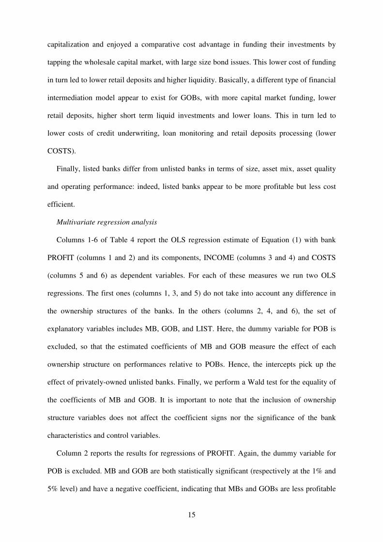
Multivariate regression analysis

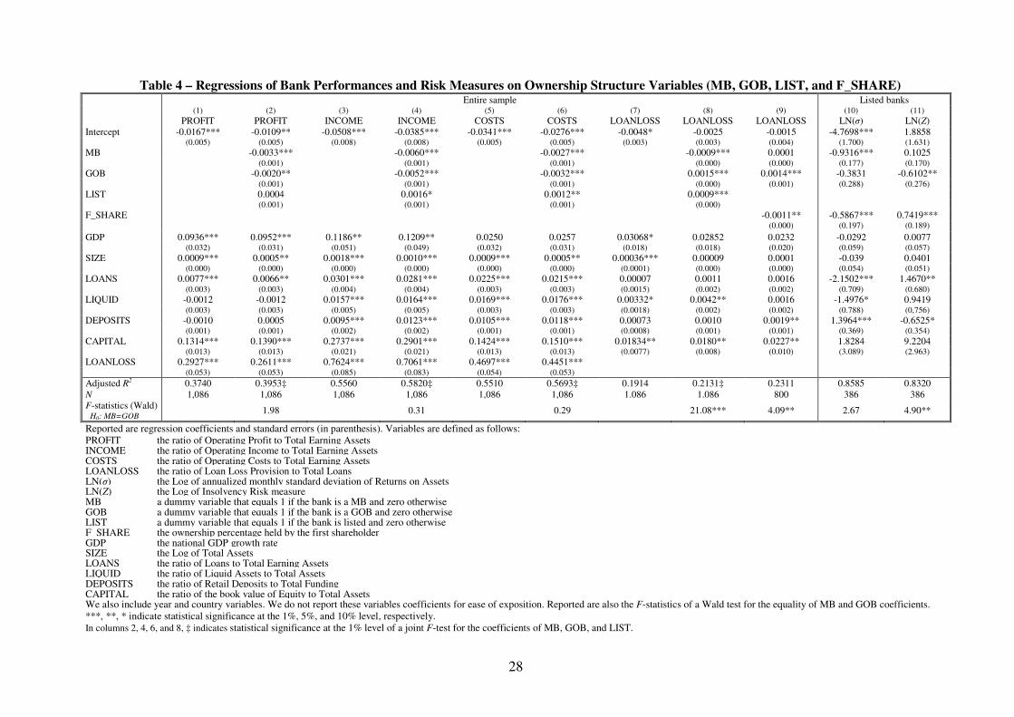
Columns 1-6 of Table 4 report the OLS regression estimate of Equation (1) with bank

PROFIT (columns 1 and 2) and its components, INCOME (columns 3 and 4) and COSTS

(columns 5 and 6) as dependent variables. For each of these measures we run two OLS

regressions. The first ones (columns 1, 3, and 5) do not take into account any difference in

the ownership structures of the banks. In the others (columns 2, 4, and 6), the set of

explanatory variables includes MB, GOB, and LIST. Here, the dummy variable for POB is

excluded, so that the estimated coefficients of MB and GOB measure the effect of each

ownership structure on performances relative to POBs. Hence, the intercepts pick up the

effect of privately-owned unlisted banks. Finally, we perform a Wald test for the equality of

the coefficients of MB and GOB. It is important to note that the inclusion of ownership

structure variables does not affect the coefficient signs nor the significance of the bank

characteristics and control variables.

Column 2 reports the results for regressions of PROFIT. Again, the dummy variable for

POB is excluded. MB and GOB are both statistically significant (respectively at the 1% and

5% level) and have a negative coefficient, indicating that MBs and GOBs are less profitable

16

than POBs after controlling for other bank characteristics. The LIST dummy variable is not

significant. The Wald test indicates that on average, GOBs and MBs do not have a

significantly different PROFIT.

Columns 4 and 6 report the results for regressions of INCOME and COSTS, respectively.

MB and GOB both have strongly significant negative coefficients, while the LIST dummy

variable has a significant (respectively at the 10% and 5% level) positive coefficient in both

regressions. These findings indicate that, on average, MBs and GOBs have both lower

INCOME and COSTS. In contrast, banks with dispersed ownership have both higher

INCOME and COSTS.

All the variables controlling for the bank characteristics have statistically significant

coefficients in both the INCOME and COSTS regression analysis. As far as PROFIT is

concerned, SIZE, LOANS, CAPITAL, and LOANLOSS all exhibit significantly positive

coefficients, while both LIQUID and DEPOSITS are not significant.

Summing up, our findings indicate that private banks are more profitable than both

mutual and public sector banks. However, this better profit performance stems from higher

net returns on their earning assets rather than from a superior cost efficiency. In fact, and

quite surprisingly, public and mutual banks’ COSTS are relatively lower. Also, public sector

banks are on average less profitable than other banks, have a larger share of their funding

coming from the wholesale interbank and capital markets, a higher liquidity and lower

investments in loans. Conversely, mutual banks appear much more similar to private banks.

They enjoy more favorable customer relationships, which in turn explain their lower

operating costs. Their lower profitability is most likely the consequence of a lower average

size and different kind of asset mix, as these banks are typically involved in more traditional

financial intermediation activities than large private banks.

4.2. Does risk taking vary according to ownership structure?

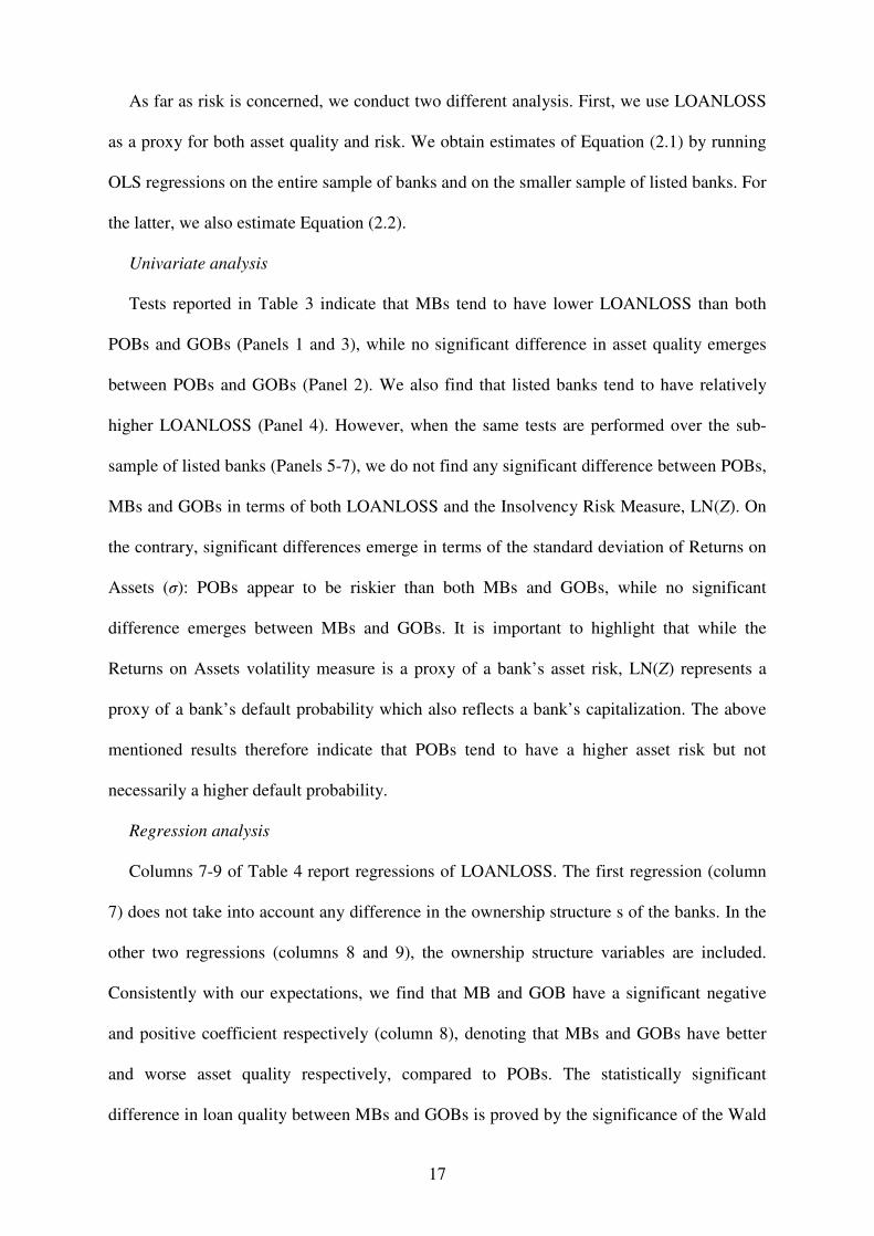
17

As far as risk is concerned, we conduct two different analysis. First, we use LOANLOSS

as a proxy for both asset quality and risk. We obtain estimates of Equation (2.1) by running

OLS regressions on the entire sample of banks and on the smaller sample of listed banks. For

the latter, we also estimate Equation (2.2).

Univariate analysis

Tests reported in Table 3 indicate that MBs tend to have lower LOANLOSS than both

POBs and GOBs (Panels 1 and 3), while no significant difference in asset quality emerges

between POBs and GOBs (Panel 2). We also find that listed banks tend to have relatively

higher LOANLOSS (Panel 4). However, when the same tests are performed over the sub-

sample of listed banks (Panels 5-7), we do not find any significant difference between POBs,

MBs and GOBs in terms of both LOANLOSS and the Insolvency Risk Measure, LN(Z). On

the contrary, significant differences emerge in terms of the standard deviation of Returns on

Assets (�): POBs appear to be riskier than both MBs and GOBs, while no significant

difference emerges between MBs and GOBs. It is important to highlight that while the

Returns on Assets volatility measure is a proxy of a bank’s asset risk, LN(Z) represents a

proxy of a bank’s default probability which also reflects a bank’s capitalization. The above

mentioned results therefore indicate that POBs tend to have a higher asset risk but not

necessarily a higher default probability.

Regression analysis

Columns 7-9 of Table 4 report regressions of LOANLOSS. The first regression (column

7) does not take into account any difference in the ownership structure s of the banks. In the

other two regressions (columns 8 and 9), the ownership structure variables are included.

Consistently with our expectations, we find that MB and GOB have a significant negative

and positive coefficient respectively (column 8), denoting that MBs and GOBs have better

and worse asset quality respectively, compared to POBs. The statistically significant

difference in loan quality between MBs and GOBs is proved by the significance of the Wald

18

test for the equality of MB and GOB coefficients. The significant positive sign of the LIST

variable denotes that on average listed banks have lower quality loans than unlisted banks.

Replacing the LIST variable with the F_SHARE variable (column 9) all the results hold with

the exception of the MB variable which loses significance19.

For the sub-sample of listed banks we use two alternative risk measures, LN(�) and

LN(Z)20. The results, reported in columns 10 and 11 of Table 4, are only partly consistent

with the ones obtained for the entire sample21. That is, MBs tend to be less risky than POBs,

while the not significant coefficient of GOB variable and the Wald test show that GOBs are

not significantly riskier than POBs nor than MBs as in the previous result (column 10).

Looking at the insolvency risk measure (column11), only GOB is significant among the

ownership structure variables, indicating a higher insolvency risk for government-owned

banks (negative coefficient signs). Once again, the difference in the results concerning the

two alternative risk variables - LN(�) and LN(Z) – can be attributed to the fact that a

different asset risk can be compensated by a different level of capitalization.

As far as the ownership concentration, consistently with regression 9, higher

concentration, measured by F_SHARE variable, produces lower risk, in terms of both LN(�)

and LN(Z).

The use of different risk proxies and different samples does not lead to unique and

unambiguous results. However, three main results emerge from our multivariate regressions.

First, public sector banks have poorer loan quality and higher insolvency risk than other

types of banks. Second, mutual banks have better loan quality and lower asset risk than both

19 Substituting the LIST variable with the F_SHARE causes a drop in the number of observations, due to the limited availability of shareholder data. 20 Since the LN(Z) is determined by the market value capital ratio while CAPITAL is a book value measure, we keep CAPITAL as a control variable. Nonetheless, no significant difference emerges in the results when excluding CAPITAL from the set of control variables. 21 We run the same kind of regressions reported in columns 1-8 (LIST is replaced with F_SHARE for these regressions) and in column 9 of Table 4 for the sub-sample of listed banks (not reported). The main results on ownership structure variable hold.

19

private and public sector banks. Finally, a higher ownership concentration is generally

associated with better loan quality, lower asset risk and lower insolvency risk.

Summing up, our results concerning risk indicate that public sector banks have poorer

loan quality and higher insolvency risk than other types of banks. This result is consistent

with the existence of conjectural or explicit government guarantees, which in turn allow

these banks to avoid the indirect costs – in terms of capital markets effects - of their poorer

asset quality and less profitable intermediation activity. On the other side, mutual banks have

better loan quality and lower asset risk than both private and public sector banks. This is

mostly the consequence of the fact that these banks enjoy more favorable customer

relationships, which in turn also explain their lower operating costs

4.3. Robustness checks

We test the robustness of our empirical results using different types of analysis.

First, since there is some evidence (Berger et al. 2000; Roland, 1997) that bank profits do

persist over time, and (Goddard et al., 2004) vary by ownership type we include a (one year)

lagged performance measure as explanatory variable in regression model (1). Results, not

reported, are similar to those obtained with the LIST dummy variable. Indeed, lagged

performance measures have a significant positive coefficient in PROFIT, INCOME, and

COSTS regressions.

Second, Goddard et al. (2004) find that there is little evidence of systematic variation in

profitability by ownership type in European countries other than Germany. Therefore, in

order to check whether our results are driven by German banks (which account for a great

number of observations) we run regressions of Table 4 excluding German bank observations.

Results, not reported, confirm our main findings.

Further, we perform the same multivariate regressions on the unbalanced sample of 1,684

bank-year observations. This sample differs from our base one, since it includes all the bank-

year observations which meet the original sample criteria without deleting any outlier or

20

bank with less than 6 year observations. Results, not reported to save space, are similar to

those obtained with our base sample.

We also use the alternative measure of ownership dispersion (for those banks for which

data are available), defined as the ownership share held by the first shareholder

(F_SHARE)22, in the regression specifications reported in columns 2, 4, and 6 of Table 4.

Results, not reported, are similar to those obtained with the LIST dummy variable23.

In addition, we use different configurations for the GOB variable (defining a bank as

GOB if a public authority holds at least 50%, 75% and 100% of its capital) without finding

any relevant difference in our results. Moreover, results (not reported) do not change by

substituting the GOB dummy variable with a continuous variable defined as the ownership

percentage held by a public authority.

Finally, since the GOB variable denotes the presence of a shareholder holding at least

25% of the bank’s equity capital, it may capture some ownership concentration effect.

Although the inclusion of the LIST variable in the regressions may be reassuring, we add the

F_SHARE variable in the regression specifications reported in Table 4, without observing

any change in both the significance and sign of the GOB variable. These results are not

reported to save space.

5. CONCLUSIONS

This paper investigates whether any significant difference exists in the performance and

risk of European banks with different ownership structure. After controlling for size, output

mix, asset quality, country and year effects, and specific macroeconomic growth

differentials, we test for systematic differences in bank performances between mutual banks,

public sector banks and private banks, and banks with different ownership concentration.

22 Shareholder information in the BankScope database are not sufficiently complete to compute any other effective and reliable measure of ownership dispersion/concentration. 23 Obviously, since LIST should proxy for banks with dispersed ownership, while F_SHARE is supposed to be positively related to ownership concentration, the signs of F_SHARE coefficients are the opposite of the LIST ones.

21

Our results confirm that significant differences in performance and risk do exist, although

their signs are not always consistent with expectations. More specifically, private banks

appear to be more profitable than both mutual and public sector banks. However, this better

profit performance stems from higher net returns on their earning assets rather than from a

superior cost efficiency. In fact, and quite surprisingly, public and mutual banks’ COSTS are

relatively lower. On the risk side, public sector banks have poorer loan quality and higher

insolvency risk than other types of banks, while mutual banks have better loan quality and

lower asset risk than both private and public sector banks.

Summing up, our findings indicate that public sector banks are on average less profitable

and riskier than other banks. Moreover, their banking activity seems to be very peculiar, with

a larger share of their funding coming from the wholesale interbank and capital markets, a

higher liquidity and lower investments in loans. This different kind of financial

intermediation model appears consistent with the existence of conjectural or explicit

government guarantees, which in turn allow these banks to avoid the indirect costs – in terms

of capital markets effects - of their poorer asset quality and less profitable intermediation

activity.

Conversely, mutual banks appear much more similar to private banks. They enjoy more

favorable customer relationships, which in turn explain both their higher loan quality and

their lower operating costs. Their lower profitability is most likely the consequence of a

lower average size and different kind of asset mix, as these banks are typically involved in

more traditional financial intermediation activities than large private banks. However, as

these types of financial institutions become increasingly involved in the same range of

activities of any private sector bank and their activities are not confined to the ones related to

the institutional objectives linked to the community they were originally set up to serve, their

peculiar ownership structure based on the “one member one vote” rule which prevents them

22

from being vulnerable to takeovers from more efficient banks becomes more and more

questionable.

These results have some relevant policy implications. If European banking regulators and

policy makers in general really aim at leveling the playing field, safeguarding banks’ asset

quality, improving the banking industry efficiency and strengthening market discipline, then

they should eliminate any form of explicit guarantee protecting public banks, clearly inform

capital market investors that no too-big-to-fail or other form of bailout policy will ever be

applied in the future for these types of banks, and remove the obstacle to the contestability of

mutual banks, which is mostly related to the “one head one vote” rule.

Finally, our results concerning the ownership concentration are quite puzzling and

deserve further research. While we find that the profitability of banks with more dispersed

owners is not significantly different from the one of more concentrated banks, we also find

that a higher ownership concentration is associated with better loan quality, lower asset risk

and lower insolvency risk. To the extent that dispersed ownership banks are found to incur

higher operating costs per euro of earning assets than concentrated ownership banks, this

finding is consistent with the agency theory prediction: however, this same theoretical

framework does not help to explain the lower loan quality and higher asset risk of banks with

a less concentrated ownership structure.

23

REFERENCES

Alchian, A.A., 1965. Some Economics of Property Rights. Il Politico, 30, 816-829.

Altunbas, Y., Molyneux, P., 1996. Economies of Scale and Scope in European Banking. Applied Financial

Economics, 6, 367-375.

Altunbas, Y., Evans, L., Molyneux, P., 2001. Bank Ownership and Efficiency. Journal of Money, Credit and

Banking, 33, 926-954.

Barth, J.R., Nolle, D.E., Phumiwasana, T., Yago G., 2003. A Cross-Country Analysis of Bank Supervisory

Framework and Bank Performance. Financial Markets, Institutions and Instruments, 12, 67-120.

Bearle, A.A., Jr., Means, G.C., 1932. The Modern Corporation and Private Property. Macmillan, New York.

Berger, A.N., 1995. The relationship between capital and earnings in banking. Journal of Money, Credit and

Banking 27, 432-456.

Berger, A.N., Humphrey, D.B., 1997. Efficiency of Financial Institutions: International Survey and Directions

for Future Research. European Journal of Operational Research, 175-212

Berger, A.N., Hanweck, G.A., Humphrey, D.B., 1987. Competitive Viability in Banking: Scale, Scope, and

Product Mix Economies. Journal of Monetary Economics, 20, 501-520.

Berger, A.N., Bonime, S.D., Covitz, D.M., Hancock, D., 2000. Why are Bank Profits so Persistent? The Roles

of Product Market Competition, Informational Opacity, and Regional/Macroeconomic Shocks. Journal of

Banking and Finance, 24, 1203-1235.

Berger, A.N., Clarke, G.R.G., Cull, R., Klapper, L., Udell, G.F., 2005. Corporate Governance and Bank

Performance: A Joint Analysis if the Static, Selection, and Dynamic Effects of Domestic, Foreign, and State

Ownership, World Bank Policy Research Working paper 3632.

Bliss, R.R., Flannery, M.J., 2000. Market Discipline in the Governance of U.S. Bank Holding Companies:

Monitoring vs. Influencing, in: Mishkin, F.S. (Ed.), Prudential Supervision: What Works and What Doesn’t,

National Bureau of Economic Research, University of Chicago Press, Chicago.

Boyd, J.H., Graham, S.L., 1988. The Profitability and Risk Effects of Allowing Bank Holding Companies to

Merge With Other Financial Firms: A Simulation Study. Federal Reserve Bank of Minneapolis Quarterly

Review, 12, 3-20.

Cordell, L., MacDonald, G., Wohar, M., 1993. Corporate Ownership and the Thrift Crisis. Journal of Law and

Economics, 36, 719-756.

Demirgüç-Kunt, A., Huizinga, H., 2001. Financial Structure and Bank Profitability, in Demirgüç-Kunt, A.,

Levine R. (editors), Financial Structure and Economic Growth: A Cross-Country Comparison of Banks,

Markets, and Development, pp. 243-261. Boston: MIT Press.

Demirgüç-Kunt, A., Huizinga, H., 1999. Determinants of Commercial Bank Interest Margins and Profitability:

Some International Evidence. The World Bank Economic Review, 13, 379-408.

Demsetz, R.S., Saidenberg, M.R., Strahan, P.E., 1997. Agency Problems and Risk Taking at Banks. Staff

Reports, No. 29. Federal Reserve Bank of New York.

De Nicolò, G., 2001. Size, Charter Value and Risk in Banking: An International Perspective. FRB International

Finance Discussion Paper No. 689.

Esty, B., 1997. Organizational Form and Risk-taking in the Savings and Loan Industry. Journal of Financial

Economics, 44, 25-55.

24

Fama, E.F., 1980. Agency Problems and the Theory of the Firm. Journal of Political Economy, 88, 288-307.

Fama, E.F., Jensen, M.C., 1983a. Separation of Ownership and Control, Journal of Law and Economics, 26,

301-325.

Fama, E.F., Jensen, M.C., 1983b. Agency Problems and Residual Claims. Journal of Law and Economics, 26,

327-349.

Flannery, M.J., 2001. The Faces of “Market Discipline”. Journal of Financial Services Research, 20, 107-119.

Fraser, D., Zardkoohi, A., 1996. Ownership Structure, Deregulation, and Risk in the Savings and Loan

Industry. Journal of Business Research, 37, 63-69.

Goddard, J., Molyneux, P., Wilson, J.O.S., 2004. The Profitability of European Banks: A Cross-Sectional and

Ddynamic Panel Analysis. The Manchester School, 72, 363-381.

Gorton, G., Rosen, R., 1995. Corporate Control, Portfolio Choice, and the Decline of Banking. Journal of

Finance, 50, 509-527.

Gropper, D.M., Beard, T.R., 1995, Insolvency, moral hazard and expense preference behavior: Evidence from

US Savings and Loan Associations. Managerial and Decision Economics 16, 606-617.

Hansmann, H., 1996. The Ownership of Enterprise. The Belknap Press of Harvard University Press,

Cambridge. MA.

Houston, J.F., James, C., 1995. CEO Compensation and Bank Risk: Is Compensation in Banking Structured to

Promote Risk Taking?. Journal of Monetary Economics, 36, 405-431.

Hughes, J.P., Mester, L.J., 1998, Bank Capitalization and Cost: Evidence of Scale Economies in Risk

Management and Signaling, The Review of Economics and Statistics, 80, 314-325.

Humphrey, D.B., 1990. Why Do Estimates of Bank Scale Economies Differ?. Federal Reserve Bank of

Richmond Economic Review, 76, 38-50.

Iannotta, G., 2006. Testing for Opaqueness in the European Banking Industry: Evidence from Bond Credit

Ratings. Journal of Financial Services Research, 30, 287-309.

Jensen, M.C., Meckling, W., 1976., Theory of the Firm: Managerial Behavior, Agency Costs, and Ownership

Structure. Journal of Financial Economics, 3, 305-360.

Kwan, S.H., 2004. Risk and Return of Publicly Held versus Privately Owned Banks. Federal Reserve Bank of

New York Economic Policy Review, 10, 97-107.

McAllister, P.H., McManus, D.A., 1993. Resolving the Scale Efficiency Puzzle in Banking. Journal of Banking

and Finance, 17, 389-405.

Mester, L., 1989. Testing for Expense Preference Behavior: Mutual versus Stock Savings and Loans. RAND

Journal of Economics, 20, 483-498.

Micco, A., Panizza, U., Yanez, M., 2004. Bank Ownership and Performance. Inter-American Development

Bank Working Paper No. 518.

O’Hara, M., 1981. Property Rights and the Financial Firm. Journal of Law and Economics, 24, 317-332.

Rasmusen, E., 1988. Mutual Banks and Stock Banks, Journal of Law and Economics, 31, 395-421.

Roland, K.P., 1997. Profit Persistence in Large US Bank Holding Companies: An Empirical Investigation.

Economics Working Paper, Office of the Comptroller of Currency.

Sapienza, P., 2004. The Effect of Government Ownership on Bank Lending. Journal of Financial Economics,

72, 357-384.

25

Saunders, A., Strock, E., Travlos, N., 1990. Ownership Structure, Deregulation and Bank Risk Taking. Journal

of Finance, 45, 643-654.

Shleifer, A., Vishny, R.W., 1997. A Survey of Corporate Governance. Journal of Finance, 52, 737-783.

Sironi, A., 2003. Testing for Market Discipline in the European Banking Industry: Evidence from Subordinated

Debt Issues. Journal of Money, Credit and Banking, 35, 443-472.

Valnek, T., 1999. The Comparative Performance of Mutual Building Societies and Stock Retail Banks. Journal

of Banking and Finance, 23, 925–938.

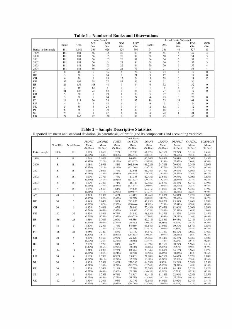
Table 1 – Number of Banks and Observations Entire Sample Listed Banks Subsample

Banks Obs. MB POB GOB LIST

Banks Obs. MB POB GOB

Obs. Obs. Obs. Obs. Obs. Obs. Obs. Banks in the sample 181 1,086 336 626 124 500 74 386 40 327 19

1999 181 181 56 105 20 80 55 55 5 47 3 2000 181 181 56 105 20 92 60 60 6 51 3 2001 181 181 56 105 20 87 64 64 5 57 2 2002 181 181 56 104 21 84 66 66 6 57 3 2003 181 181 56 103 22 84 70 70 9 57 4 2004 181 181 56 104 21 73 71 71 9 58 4

AT 8 48 6 36 6 22 5 23 4 19 0 BE 5 30 6 24 0 21 3 17 0 17 0 CH 6 36 6 18 12 24 5 28 0 11 17 DE 32 192 28 77 87 56 6 31 0 30 1 ES 26 156 108 48 0 44 6 32 0 32 0 FI 3 18 12 6 0 7 1 6 6 0 0 FR 21 126 73 53 0 34 5 27 15 12 0 GR 5 30 0 29 1 30 5 27 0 26 1 IE 5 30 6 24 0 24 4 23 0 23 0 IT 19 114 36 78 0 92 16 75 14 61 0 LU 4 24 6 12 6 3 0 0 0 0 0 NL 5 30 6 24 0 14 2 12 0 12 0 PT 6 36 0 30 6 23 3 18 0 18 0 SE 9 54 1 47 6 24 4 22 1 21 0 UK 27 162 42 120 0 82 9 45 0 45 0

Table 2 – Sample Descriptive Statistics Reported are mean and standard deviation (in parenthesis) of profit (and its components) and accounting variables.

PROFIT INCOME COSTS

Total Assets

(ml EUR) LOANS LIQUID DEPOSIT CAPITAL LOANLOSS

N. of Obs. N. of Banks Mean Mean Mean Mean Mean Mean Mean Mean Mean

(St. Dev.) (St. Dev.) (St. Dev.) (St. Dev.) (St. Dev.) (St. Dev.) (St. Dev.) (St. Dev.) (St. Dev.)

Entire sample 1,086 181 1.10% 2.86% 1.76% 109.900 61,77% 24,36% 79,27% 5,01% 0,45% (0.89%) (1.68%) (1.06%) (164.913) (20,35%) (15,11%) (21,68%) (2,35%) (0,45%)

1999 181 181 1.24% 3.10% 1.86% 86.638 60,06% 26,98% 79,91% 5,06% 0,43% (1.47%) (2.22%) (1.15%) (125.127) (19,89%) (15,58%) (22,42%) (2,66%) (0,50%)

2000 181 181 1.18% 2.99% 1.81% 102.449) 61,22% 24,70% 79,60% 5,04% 0,39% (0.97%) (1.81%) (1.11%) (151.568) (19,72%) (14,77%) (21,86%) (2,47%) (0,33%)

2001 181 181 1.06% 2.86% 1.79% 112.608 61,74% 24,17% 79,89% 4,96% 0,47% (0.68%) (1.53%) (1.04%) (168.645) (19,74%) (14,56%) (21,52%) (2,26%) (0,47%)

2002 181 181 1.00% 2.77% 1.77% 111.335 62,43% 23,68% 79,56% 4,90% 0,55% (0.64%) (1.48%) (1.02%) (158.927) (20,71%) (15,28%) (21,67%) (2,17%) (0,54%)

2003 181 181 1.07% 2.78% 1.71% 116.723 62,48% 23,57% 78,48% 5,07% 0,49% (0.66%) (1.47%) (1.03%) (174.944) (20,80%) (14,96%) (21,49%) (2,35%) (0,42%)

2004 181 181 1.04% 2.65% 1.61% 129.648 62,71% 23,06% 78,16% 5,02% 0,39% (0.61%) (1.41%) (0.99%) (199.877) (21,31%) (15,35%) (21,36%) (2,22%) (0,40%)

AT 48 8 0.78% 2.18% 1.40% 41.413 51,46% 31,85% 64,97% 3,82% 0,60% (0.43%) (1.02%) (0.65%) (51.757) (20,28%) (24,27%) (27,68%) (1,39%) (0,47%)

BE 30 5 0.84% 2.84% 1.99% 283.873 43,93% 26,82% 85,54% 3,96% 0,28% (0.22%) (1.07%) (0.92%) (120.466) (4,96%) (12,29%) (12,04%) (0,90%) (0,20%)

CH 36 6 0.82% 2.46% 1.65% 159.900 75,43% 17,65% 82,00% 5,00% 0,39% (0.24%) (0.65%) (0.62%) (318.800 (23,35%) (22,88%) (10,38%) (1,68%) (1,00%)

DE 192 32 0.43% 1.19% 0.77% 124.800 48,93% 34,37% 61,37% 2,68% 0,45% (0.26%) (0.75%) (0.63%) (149.723) (17,96%) (13,99%) (28,11%) (1,16%) (0,49%)

ES 156 26 1.61% 3.70% 2.09% 46.586 69,71% 22,83% 89,43% 7,21% 0,45% (0.49%) (0.94%) (0.59%) (86.410) (10,92%) (8,81%) (8,91%) (2,41%) (0,26%)

FI 18 3 1.47% 3.23% 1.76% 64.089 66,54% 21,08% 90,30% 6,87% 0,05% (0.54%) (1.14%) (0.70%) (69.178) (13,51%) (12,06%) (4,88%) (2,44%) (0,13%)

FR 126 21 0.85% 2.74% 1.88% 193.752 44,17% 31,33% 88,39% 3,88% 0,46% (0.57%) (1.61%) (1.09%) (207.653) (19,92%) (14,97%) (13,66%) (1,56%) (0,28%)

GR 30 5 2.19% 5.16% 2.97% 26.478 55,96% 35,44% 96,33% 8,02% 0,92% (1.07%) (1.36%) (0.58%) (14.047) (13,47%) (11,44%) (6,00%) (2,91%) (0,22%)

IE 30 5 2.09% 3.92% 1.84% 46.261 69,39% 18,76% 90,77% 5,56% 0,21% (3.12%) (3.66%) (0.99%) (34.545) (7,87%) (5,86%) (9,53%) (0,90%) (0,19%)

IT 114 19 1.31% 4.03% 2.72% 69.544 70,34% 22,68% 74,15% 3,66% 0,77% (0.64%) (1.05%) (0.74%) (81.761) (8,70%) (7,15%) (11,03%) (1,05%) (0,46%)

LU 24 4 0.69% 1.59% 0.90% 23.803 21,90% 44,76% 84,62% 6,77% 0,18% (0.37%) (0.61%) (0.29%) (12.202) (6,17%) (6,74%) (12,30%) (2,36%) (0,36%)

NL 30 5 0.83% 3.29% 2.46% 230.266 64,39% 8,83% 63,29% 5,38% 0,25% (0.61%) (1.50%) (1.71%) (282.579) (12,76%) (2,66%) (24,51%) (1,48%) (0,18%)

PT 36 6 1.35% 3.54% 2.19% 37.289 75,29% 15,93% 84,11% 5,52% 0,62% (0.27%) (0.49%) (0.40%) (21.299) (10,45%) (6,09%) (7,70%) (0,92%) (0,25%)

SE 54 9 0.99% 1.73% 0.74% 78.367 86,41% 11,14% 52,96% 4,23% 0,05% (0.27%) (0.85%) (0.77%) (68.755) (13,30%) (10,71%) (25,25%) (0,92%) (0,09%)

UK 162 27 1.33% 3.26% 1.93% 142.793 73,68% 14,02% 93,02% 5,24% 0,41% (0.93%) (1.79%) (1.07%) (204.763) (13,36%) (10,07%) (8,11%) (1,41%) (0,48%)

Table 3 – Bivariate Comparison of Bank Performances, Control Variables and Risk Measures

Entire sample Listed Banks Subsample

Panel 1 Panel 2 Panel 3 Panel 4 Panel 5 Panel 6 Panel 7 (GOBs excluded) (MBs excluded) (POBs excluded) (All banks) (GOBs excluded) (MBs excluded) (POBs excluded) MBs POBs GOBs POBs MBs GOBs LIST NON-LIST MBs POBs GOBs POBs MBs GOBs

[t statistic] [t statistic] [t statistic] [t statistic] [t statistic] [t statistic] [t statistic] PROFIT 1.05% 1.24% 0.52% 1.24% 1.05% 0.52% 1.28 0.95% 0.84% 1.29% 0.64% 1.29% 0.84% 0.64% [-3.550]*** [-14.270]*** [12.748]*** [6.089]*** [-6.072]*** [-4.184]*** [1.913]**

INCOME 2.89% 3.14% 1.36% 3.14% 2.89% 1.36% 3.31% 2.47% 2.78% 3.45% 2.28% 3.45% 2.78% 2.28% [-2.362]** [-17.635]*** [15.316]*** [8.452]*** [-2.919]*** [-9.347]*** [2.527]**

COSTS 1.84% 1.90% 0.84% 1.90% 1.84% 0.84% 2.03% 1.52% 1.93% 3.45% 1.64% 3.45% 1.93% 1.64% [-0.855] [-15.351]*** [13.884]*** [8.364]*** [-1.353] [-5.410]*** [1.805]**

Total Assets 70,621 132,441 102,540 131,441 70,621 102,540 156,927 69,775 109,819 182,539 23,314 182,539 109,819 23,314 [-6.257]*** [-2.447]** [-2.701]*** [8.550]*** [-2.294]** [-11.144]** [2.917]***

CAPITAL 5.82% 4.88% 3.48% 4.88% 5.82% 3.48% 5.24% 4.81% 5.18% 5.18% 5.71% 5.18% 5.18% 5.71% [5.673]*** [-8.470]*** [11.681]*** [3.074]*** [-0.013] [1.126] [-1.056]

LOANS 62.77% 64.07% 47.45% 64.07% 62.77% 47.45% 62.55% 61.11% 53.30% 63.47% 78.86% 63.47% 53.30% 78.86% [-1.005] [-7.372]*** [7.198]*** [1.207] [-3.374]*** [4.776]*** [-5.841]***

LIQUID 23.60% 22.72% 34.71% 22.72% 23.60% 34.71% 23.15% 25.39% 30.11% 22.54% 12.12% 22.54% 30.11% 12.12% [0.910] [7.187]*** [-6.441]*** [-2.505]** [4.118]*** [-4.003]*** [6.703]***

DEPOSITS 88.41% 76.68% 67.59% 76.68% 88.41% 67.59% 81.25% 77.58% 79.99% 79.34% 75.29% 79.34% 79.99% 75.29% [9.608]*** [-4.057]*** [9.893]*** [2.869]*** [0.046]*** [-1.047] [1.353]

LOANLOSS 0.38% 0.47% 0.55% 0.47% 0.38% 0.55% 0.54% 0.38% 0.53% 0.54% 0.91% 0.54% 0.53% 0.91% [-3.328]*** [1.070] [-2.327]** [5.973]*** [-0.142] [1.135] [-1.130] � 0.001% 0.043% 0.38% 0.043% 0.001% 0.38% [-6.452]*** [6.426]*** [-1.110] Z 12,241 9,778 13,497 9,778 12,241 13,497

[0.514] [0.539] [-0.201]

Reported are mean values of performance measures and control variables of Mutual Banks (MBs), Privately-Owned Banks (POBs), Government-Owned Banks (GOBs), and listed (LIST) and unlisted (NON-LIST) banks, for both the Entire sample and the Listed Banks Subsample. The value in square brackets is the t-statistic for testing the equality of variable means. Variables are defined as follows: PROFIT the ratio of Operating Profit to Total Earning Assets

INCOME the ratio of Operating Income to Total Earning Assets

COSTS the ratio of Operating Costs to Total Earning Assets

Total Assets the book value of Total Assets in millions of euro

CAPITAL the ratio of the book value of Equity to Total Assets

LOANS the ratio of Loans to Total Earning Assets

LIQUID the ratio of Liquid Assets to Total Assets

DEPOSITS the ratio of Retail Deposits to Total Funding

LOANLOSS the ratio of Loan Loss Provision to Total Loans

� the annualized monthly standard deviation of Returns on Assets

Z the Insolvency Risk measure

***, **, * indicate statistical significance at the 1%, 5% and 10% level, respectively.

28

Table 4 – Regressions of Bank Performances and Risk Measures on Ownership Structure Variables (MB, GOB, LIST, and F_SHARE)

Entire sample Listed banks (1) (2) (3) (4) (5) (6) (7) (8) (9) (10) (11) PROFIT PROFIT INCOME INCOME COSTS COSTS LOANLOSS LOANLOSS LOANLOSS LN(�) LN(Z)

Intercept -0.0167*** -0.0109** -0.0508*** -0.0385*** -0.0341*** -0.0276*** -0.0048* -0.0025 -0.0015 -4.7698*** 1.8858 (0.005) (0.005) (0.008) (0.008) (0.005) (0.005) (0.003) (0.003) (0.004) (1.700) (1.631)

MB -0.0033*** -0.0060*** -0.0027*** -0.0009*** 0.0001 -0.9316*** 0.1025 (0.001) (0.001) (0.001) (0.000) (0.000) (0.177) (0.170)

GOB -0.0020** -0.0052*** -0.0032*** 0.0015*** 0.0014*** -0.3831 -0.6102** (0.001) (0.001) (0.001) (0.000) (0.001) (0.288) (0.276)

LIST 0.0004 0.0016* 0.0012** 0.0009*** (0.001) (0.001) (0.001) (0.000)

F_SHARE -0.0011** -0.5867*** 0.7419*** (0.000) (0.197) (0.189)

GDP 0.0936*** 0.0952*** 0.1186** 0.1209** 0.0250 0.0257 0.03068* 0.02852 0.0232 -0.0292 0.0077 (0.032) (0.031) (0.051) (0.049) (0.032) (0.031) (0.018) (0.018) (0.020) (0.059) (0.057)

SIZE 0.0009*** 0.0005** 0.0018*** 0.0010*** 0.0009*** 0.0005** 0.00036*** 0.00009 0.0001 -0.039 0.0401 (0.000) (0.000) (0.000) (0.000) (0.000) (0.000) (0.0001) (0.000) (0.000) (0.054) (0.051)

LOANS 0.0077*** 0.0066** 0.0301*** 0.0281*** 0.0225*** 0.0215*** 0.00007 0.0011 0.0016 -2.1502*** 1.4670** (0.003) (0.003) (0.004) (0.004) (0.003) (0.003) (0.0015) (0.002) (0.002) (0.709) (0.680)

LIQUID -0.0012 -0.0012 0.0157*** 0.0164*** 0.0169*** 0.0176*** 0.00332* 0.0042** 0.0016 -1.4976* 0.9419 (0.003) (0.003) (0.005) (0.005) (0.003) (0.003) (0.0018) (0.002) (0.002) (0.788) (0,756)

DEPOSITS -0.0010 0.0005 0.0095*** 0.0123*** 0.0105*** 0.0118*** 0.00073 0.0010 0.0019** 1.3964*** -0.6525* (0.001) (0.001) (0.002) (0.002) (0.001) (0.001) (0.0008) (0.001) (0.001) (0.369) (0.354)

CAPITAL 0.1314*** 0.1390*** 0.2737*** 0.2901*** 0.1424*** 0.1510*** 0.01834** 0.0180** 0.0227** 1.8284 9.2204 (0.013) (0.013) (0.021) (0.021) (0.013) (0.013) (0.0077) (0.008) (0.010) (3.089) (2.963)

LOANLOSS 0.2927*** 0.2611*** 0.7624*** 0.7061*** 0.4697*** 0.4451*** (0.053) (0.053) (0.085) (0.083) (0.054) (0.053)

Adjusted R2 0.3740 0.3953‡ 0.5560 0.5820‡ 0.5510 0.5693‡ 0.1914 0.2131‡ 0.2311 0.8585 0.8320 N 1,086 1,086 1,086 1,086 1,086 1,086 1.086 1.086 800 386 386 F-statistics (Wald)

H0: MB=GOB 1.98 0.31 0.29 21.08*** 4.09** 2.67 4.90**

Reported are regression coefficients and standard errors (in parenthesis). Variables are defined as follows: PROFIT the ratio of Operating Profit to Total Earning Assets INCOME the ratio of Operating Income to Total Earning Assets COSTS the ratio of Operating Costs to Total Earning Assets LOANLOSS the ratio of Loan Loss Provision to Total Loans LN(�) the Log of annualized monthly standard deviation of Returns on Assets LN(Z) the Log of Insolvency Risk measure MB a dummy variable that equals 1 if the bank is a MB and zero otherwise GOB a dummy variable that equals 1 if the bank is a GOB and zero otherwise LIST a dummy variable that equals 1 if the bank is listed and zero otherwise F_SHARE the ownership percentage held by the first shareholder GDP the national GDP growth rate SIZE the Log of Total Assets LOANS the ratio of Loans to Total Earning Assets LIQUID the ratio of Liquid Assets to Total Assets DEPOSITS the ratio of Retail Deposits to Total Funding CAPITAL the ratio of the book value of Equity to Total Assets We also include year and country variables. We do not report these variables coefficients for ease of exposition. Reported are also the F-statistics of a Wald test for the equality of MB and GOB coefficients. ***, **, * indicate statistical significance at the 1%, 5%, and 10% level, respectively. In columns 2, 4, 6, and 8, ‡ indicates statistical significance at the 1% level of a joint F-test for the coefficients of MB, GOB, and LIST.