OOvveerrvviieeww

Softcopy photogrammetry is the science of obtaining reliable measurements and maps from photographs. It is a type of remote sensing that makes use of cameras to vertically photograph the surface and produce accurate topographic image maps.

Although both maps and aerial photography represent a portion of the earth’s surface, aerial photographs are not considered maps. Unlike maps, which depict the landscape with generalized symbols and colors, aerial photography reveals the actual surface terrain. Forests, fields, buildings, roads and other man-made features are depicted as they were at the actual time that the photographs were taken. Physical features represented within the photograph contain detail that no map can depict, and can represent a moment in the history of a location. Land use changes can be easily recorded by using photos from the same area taken at different times.

A major disadvantage of aerial photos is that they display a high degree of radial topographical distortion, and scale variations. Until corrections are made for the distortion, measurements made from a photograph are not accurate, unlike maps that are directionally and geometrically accurate. The distortion and scale variations are caused by small tilts in the camera and movement of the aircraft during the time of capture, as well as by natural variations in the elevation of the terrain. Once these variations in scale are removed from the photo, it can become a true image-map with a constant scale representation of a portion of the surface.

Figure 1 – Schematic diagram showing typical relief distortion from an aerial photograph, (right) compared to a typical map projection (left) (source: Lillesand & Kiefer, 1994).

The process of removing the distortions and scale variations from aerial photography is known as orthorectification. This process also gives the image geo-referencing, so that the photo is geo-coded with a map projection, and can be integrated with other map data in a GIS (Geographic Information System). Another advantage of orthorectification is that many of the orthorectified images can be mosaicked together to form a larger seamless image-map.

PCI Geomatica OrthoEngine is a powerful photogrammetric tool designed to efficiently produce quality orthorectified geospatial image products using various rigerous math models. A math model is a mathematical relationship used to correlate the pixels of an image to correct locations on the ground accounting for known distortions. The math model choosen will directly impact the resultant outcome. This project evaluates two of PCI’s orthorectification math models to correct both traditional and digital aerial photography; the Aerial Photography model and the Thin Plate Spline Model.

The traditional photos for this project were captured with a standard RC 10 aerial mapping frame camera. Nova Scotia 1:10,000 topographic map sheets are based on black and white 1:40,000 aerial photography flown with leaf off conditions. Three of these photos from the Middleton area were selected for the first part of this project. Two photos were adjacent one another, selected from the same flight line and the third from the flight line north of it. All photos were actual paper copys and had to be input into the computer using a digital scanner.

Figure 2 – The components of a standard RC 20 aerial mapping camera (left) and a schematic diagram showing the principle components of the camera setup (right) (source: Lillesand & Kiefer, 1994).

AAeerriiaall PPhhoottooggrraapphhyy MMooddeell

The aerial photography model is based on the geometry of a standard aerial photography frame camera. This model incorporates the curvature of the lens, focal length, focal point, topographic variations and the position of the camera when the photograph was taken. The exact position and orientation of the camera when the image was taken is known as the exterior orientation, and is used during the computation of this model. It can be more clearly defined as the relationship between the image orientation and the exact orientation of the surface. Traditional cameras capture a negative image and then require further processing of the image to produce a positive image that is the actual representation of the surface. Six different parameters make up the exterior orientation and are often defined as the x axis, the y axis, the z axis, phi, kappa, and omega. Phi, kappa, and omega are the angles that define the axis of x, y, z.

Figure 3 – Schematic diagram demonstrating the six parameters that make up the exterior orientation of an aerial photography camera (source: PCI help file).

For traditional aerial photography, the cameras have been calibrated to help correct any lens distortion. For each flight, a camera calibration report with details about the camera that was used to take the aerial photograph is recorded. To help define the exterior orientation of the camera, these basic details must be provided such as the focal length, principal point offset, radial lens distortion values (if available), photo scale, and distance between the fiducial marks. This data is usually provided with the camera calibration report. The camera calibration report data helps increases the accuracy of the model, but is not absolutely necessary. If a camera calibration report is not available, approximate values can be used in place of the unknown camera parameters. Approximate values such the focal length are often recorded on one of the sides of the photograph. Traditional aerial photographs contain fiducial marks to aid in the calibration of the focal point, and help establish the photo coordinate system. Fiducial marks are small crosses or small V-shaped indents located precisely on each of the four corners or halfway along the four edges of the photograph.

Figure 4 – Standard aerial photography such as this 1:40,000 black and white photograph has fiducial marks (left image) on the four corners and the four edges that help define the exterior orientation of the camera. The principal point is the intersection of the imaginary perpendicular lines

that intersect through the center of the image. The camera distortions often cause this point to be slightly off from the center of photography. The actual principal point position of the photo is determined from the measurements of the fiducial marks.

Figure 5 – Schematic diagram demonstrating the focal point and focal length that determine the principal point of an aerial photography camera (source: PCI help file).

The AGRG has been involved with an extensive high resolution aerial photograph mission over the past year. This photography has been collected for many different research purposes such as providing high resolution imagery for the validation of the acquired LIDAR data that was collected during the spring of 2003. The digital camera used for the capture of the photography is not a highly calibrated camera, but still has important information that must be included to compute the model. Digital photographs, unlike traditional photographs, do not contain fiducial marks so the focal length and the size of the CCD (Charged Coupled Device) is used to calculate the geometry of the exterior orientation. A CCD is a micro electric silicon chip, a solid-state sensor that detects electromagnetic energy. When this energy strikes the CCD’s silicon surface, electronic charges are produced, with the magnitude of the charges being proportional to the scene brightness (Lillesand & Kiefer, 1994). Digital photographs are not usually square shaped like traditional photographs are, thus the software must convert the image to a normalized coordinate system in order to compute the math model. The resultant photos are also already in digital format thus no scanning process is required.

Figure 6 – Raw digital aerial photo, approximate coverage of 1500 m by 1000 m.

The aerial photography math model transforms the exterior orientation of

the photograph into a known ground coordinate system. Ground control points (GCPs) and tie points are both required to compute the triangulation solution of the exterior orientation of the camera. This model requires about four precise GCPs per image.

Ground control points are identifiable features in the image that have

known three dimensional ground coordinates. These can be obtained from a vector layer, a georeferenced image or GPS data. The GCPs help determine the relationship between the image and the ground by relating the pixels and lines of the image to the coordinates on the ground. Good examples of GCP sources are road intersections, and any identifiable man made feature such as photo targets.

Figure 7 – A GCP is a known point that is identifiable on the image and has known geographic coordinates (source: PCI help file). Targets are often placed on the ground prior to an aerial photography

mission to help provide accurate ground postions. Most often a target will be made of bright white material and placed in the shape of a X or a Y, with the geometric coordinates of the center recorded with a GPS.

Figure 8 – Two examples of targets used to provide accurate ground control for aerial photography missions. (source: AGRG). Tie points are features that occur on two or more photos that do not have

known geometric coordinates but are similar with limited distortion. Tie points help identify how the images relate to each other. They are really important in areas that have few GCPs and ensure that the best fit for the individual images, as well as the in the calculation of the model. It is important to avoid features that

often have known distortion such as trees and buildings, good tie points are usually exposed rocks or asphalt patches on paved roads.

Figure 9 – A tie point is a known point that is identifiable on two images that doesn’t need to have known geographic coordinates (source: PCI help file).

The re-creation of the exterior orientation transformation from the

computation with the coordinates provided from the GCPs and tie points will generate the overall model that will be applied to the images in order to remove the geometric distortions and give it spatial reference. The mosaicked photos together can provide an image product that has both visual and geometric information and can be integrated with other spatial data in a GIS.

TThhiinn PPllaattee SSpplliinnee MMooddeell

The name "thin plate spline" refers to a physical analogy involving the bending of a thin sheet of metal. In the physical setting, the deflection is in the z direction, orthogonal to the plane. In order to apply this idea to the problem of coordinate transformation, one interprets the lifting of the plate as a displacement of the x or y coordinates within the plane (Weisstein, 2003).

This model is a fairly simple model in which all the collected GCPs are used simultaneously to compute the final transformation. A warping effect is distributed throughout the image with extrapolation error between the GCPs becoming almost linear away from the GCPs. This also means that the math model does not provide direct means of detecting and correcting distortions in the image.

This method is not recommended for large scale applications and to account for the warping transformation effect, the user must make sure that there is an addequate amount of GCPS collected across the entire image. This model doesn’t require camera calibration information or the collection of tie points like the aerial photography model does.

.

Figure 10 – A mathematical graphical representation of how the thin plate spline model bends an image to fit the control points provided (source: http://folk.uio.no/ohammer/past/screens.html).

PPrroocceessssiinngg PPrroocceedduurreess

Select a math model

Set the Projetion

Import Image

Collect tie points

Compute the math model / Generate orthophotos

Mosaic photos

Collect GCPS

Figure 11 – General flow chart Procedure for mosaicking aerial photography .

The following is a brief overview of the processing procedures used to produce orthorectified mosaic files of the aerial photographs. (More details can be found with PCI help files)

AAeerriiaall PPhhoottooggrraapphhyy MMaatthh MMooddeell

1) Setup Project File

Figure 12 – Project information window with sample input.

• •

Enter a filename, name and description of project Select the math model, camera type and method of computing the exterior orientation

Figure 13 – Set Projection window with sample input.

• Enter projection information for the output orthorectified photos, and the projection for the data that the GCPs will be selected from

Set the size of the image pixel •• •• You can set the GCP selection by pressing the “Set GCP Projection …” button

if they both projections are the same

Figure 14 – Camera Calibration window with sample input.

•• Enter the information provided with the calibration report; focal length (required), principal point offset (optional), distortion coefficient values (optional), photo scale (optional), and earth radius (optional)

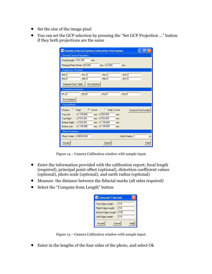
•• Measure the distance between the fiducial marks (all sides required) •• Select the “Compute from Length” button

Figure 15 – Camera Calibration window with sample input.

Enter in the lengths of the four sides of the photo, and select Ok ••

•• The Fiducial coordinates boxes should fill in based on the information you provided

2) Input Image

Figure 16 – Open Photo window with sample input.

•• Click the “Open a new or existing photo” icon, to open the Open Photo window

•• When importing an image to the project for the first time, you need to click the New Photo button and select your image file

Figure 17 – Center of a fiducial mark on a traditional aerial photo.

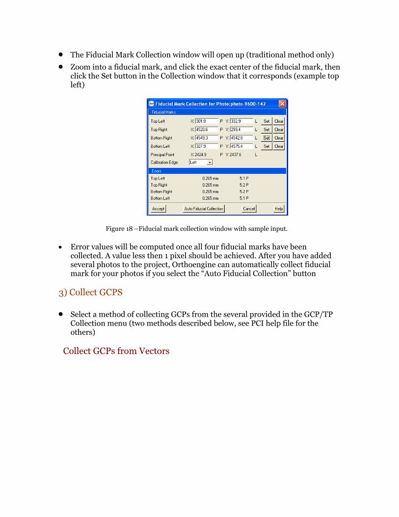
The Fiducial Mark Collection window will open up (traditional method only) •• •• Zoom into a fiducial mark, and click the exact center of the fiducial mark, then

click the Set button in the Collection window that it corresponds (example top left)

•

••

Figure 18 –Fiducial mark collection window with sample input.

Error values will be computed once all four fiducial marks have been collected. A value less then 1 pixel should be achieved. After you have added several photos to the project, Orthoengine can automatically collect fiducial mark for your photos if you select the “Auto Fiducial Collection” button

3) Collect GCPS

Select a method of collecting GCPs from the several provided in the GCP/TP Collection menu (two methods described below, see PCI help file for the others)

Collect GCPs from Vectors

•• Load an image to collect GCPs •• Load a vector file to collect

coordinates from •• Load a digital elevation model

(DEM) to derive orthometric heights from

•• Make sure the bundle adjustment check box is selected (this will automatically update the model as GCPs are added to the project

Figure 19 –Collect GCPs from vectors window after 1 GCP has been collected.

••

Figure 20 – Vector file (left) with a road intersection selected for a GCP and the corresponding location on the aerial photograph (right)

Select a position on the image to use as a GCP, select “Use Point” button •• Find the same position in the vector layer to use as the GCP, select “Use

Point” button •• Select the “Extract Elevation” button •• Select the “Accept” button • •

••

Continue to collect 3 to 4 more GCPs A residual error will appear in the bottom portion of the GCP collection window after 4 points have been collected

An acceptable error value of less then 1 pixel is desired •• If the error is really high, delete the GCP that is causing the problem and

continue collecting a few more till the error is acceptable. (Note: collecting a lot of GCPs will not necessarily reduce the error)

Collect GCPs from Geocoded Image

•• Load an image to collect GCPs from

•• Load a geocoded image to collect coordinates from

•• Load a digital elevation model (DEM) to derive orthometric heights from

•• Make sure the bundle adjustment check box is selected (this will automatically update the model as GCPs are added to the project

Figure 21 –Collect GCPs from geocoded image window after 4 GCPs have been collected.

••

Figure 22 – Geocoded image (left) with a vector file opened to help find the exact location. The same area in the image (right) where the GCP will be collected.

Select a position on the image to use as a GCP, select “Use Point” button •• Find the same position in the geocoded image to use as the GCP, select “Use

Point” button •• Select the “Extract Elevation” •• Select the “Accept” button • •

••

Continue to collect 3 to 4 more GCPs A residual error will appear in the bottom portion of the GCP collection window after 4 points have been collected

An acceptable error value of less then 1 pixel is desired •• If the error is really high, delete the GCP that is causing the problem and

continue collecting a few more till the error is acceptable. (Note: collecting a lot of GCPs will not necessarily reduce the error)

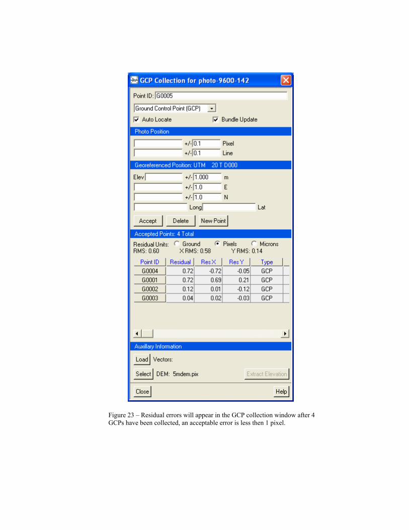
Figure 23 – Residual errors will appear in the GCP collection window after 4 GCPs have been collected, an acceptable error is less then 1 pixel.

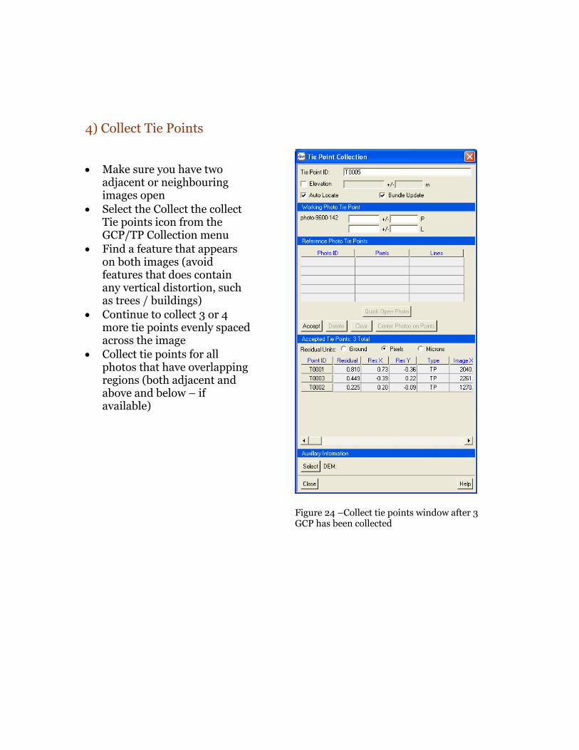
4) Collect Tie Points

•

•

•

•

•

Make sure you have two adjacent or neighbouring images open Select the Collect the collect Tie points icon from the GCP/TP Collection menu Find a feature that appears on both images (avoid features that does contain any vertical distortion, such as trees / buildings) Continue to collect 3 or 4 more tie points evenly spaced across the image Collect tie points for all photos that have overlapping regions (both adjacent and above and below – if available)

Figure 24 –Collect tie points window after 3 GCP has been collected

Figure 25 – Two images displaying a bare patch of soil that can be used as a common tie point feature.

4) Generate Ortho Photos

Select the “Schedule Ortho Generation icon” from the Ortho Generation menu •• •• Highlight the images from the available photos frame on the left and click the

right arrow button •• The photos should then appear on the right side frame in the process photos

window •• Load the DEM •• Select the Processing Option •• Click “Generate Orthos” button

Figure 26 – The Ortho Photo Production window where all parameters are set prior to orthophoto generation.

5) View Orthophoto

Select Image View from File in the main menu ••

Figure 27 – Image View option.

•• Browse to find your orthorectified image file and load the image, then add vectors on top and look to see that the orthorectified image was created successfully

Figure 28 – Ortho rectified image displayed with the Image View option.

5) Mosaic Ortho Photos

Figure 29 – Mosaic icons.

•• After the orthorectified photos have been generated go to the Mosaic menu, select Define Mosaic Area icon

•• The Define Mosaic Area window will contain black silhouettes of your orthorectified images to give you an idea of their geometric orientation to each other

•• Hold down on the shift key and then click and drag a box over the images •• A white box should appear with the coordinates of the extent of the mosaic file

automatically filled in the appropriate boxes on the left •• Select the Create Mosaic File button and give the mosaic file a name

Figure 30 –Hold the shift key and then click and drag a box in the Define Mosaic Area window (left) and then the extent of the mosaic file with coordinates will appear (right).

Open the Automatic Mosaicking window •• •• Select the images that you wish to add to the mosaic •• Select Generate Mosaic button

Figure 31 – Automatic mosaicking window.

Digital Photos

•• The process for the digital photos are the same as the above procedure with the following exceptions

•• The Digital / Video option is selected when choosing the Math Model •• Fill in the focal length and the chip size in the Camera Calibration Window

Figure 32 – Project information window.

Figure 33 – Camera Calibration window for the digital camera.

TThhiinn PPllaattee SSpplliinnee MMaatthh MMooddeell

1) Setup Project File

• •

Figure 34 – Project information window for Thin Plate Spline method with sample input.

Enter a filename, name and description of project Select the math model, camera type and method of computing the exterior orientation

Figure 35 – Set Projection window with sample input.

•

••

Enter projection information for the output orthorectified photos, and the projection for the data that the GCPs will be selected from

Set the size of the image pixel •• Load images, collect GCPs, create orthorectified images, mosaic files together

(all these steps are the same as the above method except there are no Collect tie points option)

VVaalliiddaattiioonn // AAnnaallyyssiiss

After the photos have been orthorectified and mosaicked together it is important to validate the resultant images to ensure that the photos have been properly georeferenced and orthorectified. The images can be exported as geo-tiffs with PCI’s File Utility feature. The tiff files can then be integrated with GIS data. ESRI ArcGIS 9 was used to evaluate the images. The mosaicked image files were opened up with ArcMap along, with vector files, digital surface models created from the LIDAR data, and the LIDAR DEM (ground hits). Visible features such as roads, trees, and building were examined to compare the fit of the image. The traditional 1:40,000 aerial images from the calibrated frame camera matched with the vector layers and the LIDAR, and were never off more then 1meter. At first glance the AGRG digital image appeared to have been accurately corrected, but after a zoomed in closer examination, it was determined that some parts of the photo were off by 6 to meters. This error was expected due to the fact that the exact calibrated camera information was not available (rather an estimate value, e.g. focal length). The thin plate spline method helped give the image a better fit in areas where the traditional aerial photography model could not, but sometimes caused more error in the image. Thus one should be cautious with this method because although it may give a better fit most of the time, it can also warp the image causing other errors. Using the Thin Plate Spline method with the orthorectified images produced from the standard aerial photograph model helped to create a more accurate image mosaic of the AGRG digital photos.

Figure 35 – Examination of the orthorectified images using ArcGIS9, the images both seem to have been properly corrected. (Top left) Key map showing location of zoomed in areas, shaded relief model of the all-hits LIDAR grid with a road vector over laid on top (right top), AGRG digital photos orthorectified using the standard aerial photo model (bottom left), and the AGRG digital photos orthorectified with the spline method, (bottom right).

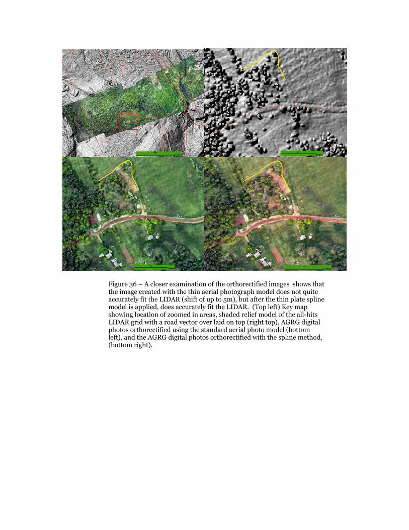
Figure 36 – A closer examination of the orthorectified images shows that the image created with the thin aerial photograph model does not quite accurately fit the LIDAR (shift of up to 5m), but after the thin plate spline model is applied, does accurately fit the LIDAR. (Top left) Key map showing location of zoomed in areas, shaded relief model of the all-hits LIDAR grid with a road vector over laid on top (right top), AGRG digital photos orthorectified using the standard aerial photo model (bottom left), and the AGRG digital photos orthorectified with the spline method, (bottom right).

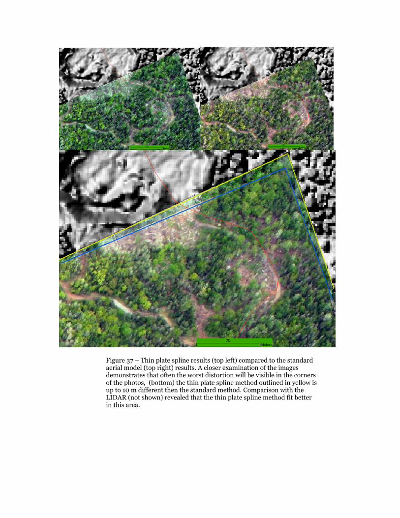
Figure 37 – Thin plate spline results (top left) compared to the standard aerial model (top right) results. A closer examination of the images demonstrates that often the worst distortion will be visible in the corners of the photos, (bottom) the thin plate spline method outlined in yellow is up to 10 m different then the standard method. Comparison with the LIDAR (not shown) revealed that the thin plate spline method fit better in this area.

Figure 38 – Final mosaicked image using the standard aerial photography model overtop of the LIDAR all hits shaded surface.

Figure 39 – Final mosaicked image using the standard aerial photography model and then further processing using the thin plate spline model to achieve a better more accurate fit to the LIDAR all hits shaded surface.

RReeffeerreenncceess

Lillesand, T. and R. Kiefer (1994). Remote Sensing and Image Interpretation. NewYork: John Wiley & Sons, Inc.

PCI Geomatics (2003). Othoengine help files.

Weisstein, E. W. (2003). Wolfram Research, Inc. Retrieved December 8, 2003 from http://mathworld.wolfram.com/ThinPlateSpline.html