Overview: Simulating (coupled) reactive multi-component transport with PHT3D

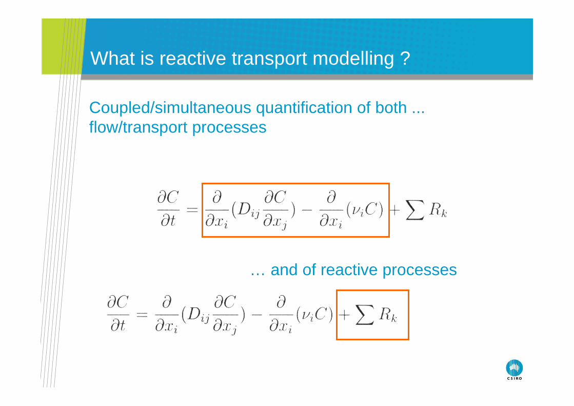
What is reactive transport modelling ?

Coupled/simultaneous quantification of both ...flow/transport processes

… and of reactive processes

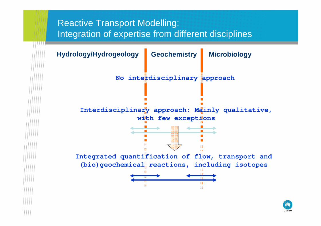
Hydrology/Hydrogeology Geochemistry Microbiology

Interdisciplinary approach: Mainly qualitative, with few exceptions

No interdisciplinary approach

Integrated quantification of flow, transport and (bio)geochemical reactions, including isotopes

Reactive Transport Modelling: Integration of expertise from different disciplines

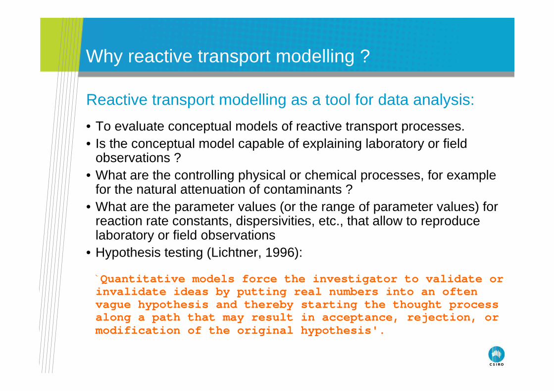
Why reactive transport modelling ?

Reactive transport modelling as a tool for data analysis:

• To evaluate conceptual models of reactive transport processes. • Is the conceptual model capable of explaining laboratory or field

observations ?• What are the controlling physical or chemical processes, for example

for the natural attenuation of contaminants ?• What are the parameter values (or the range of parameter values) for

reaction rate constants, dispersivities, etc., that allow to reproduce laboratory or field observations

• Hypothesis testing (Lichtner, 1996):

` Quantitative models force the investigator to valid ate or invalidate ideas by putting real numbers into an of ten vague hypothesis and thereby starting the thought p rocess along a path that may result in acceptance, rejecti on, or modification of the original hypothesis'.

Why reactive transport modelling ?

Reactive transport modelling as predictive tool:• To what extent will environmentally important receptors downgradient

of the source zone be impacted by a contaminant ?• What are maximum concentration levels and what is the contaminant

mass flux ?• What are the time-scales for cleanup to below given limits for different

remediation schemes ?• What is the optimal design of a particular (active/passive) remediation

scheme ?

However, predictions are strongly effected by uncertainty that originates from:

• Incomplete hydrogeological and hydrogeochemical site characterization

• Incomplete or completely unknown ‘source’ history• Incomplete process understanding, wrong conceptual models

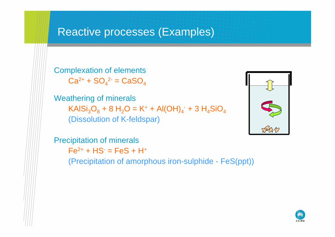
Complexation of elements Ca2+ + SO4

2- = CaSO4

Weathering of minerals KAlSi3O8 + 8 H2O = K+ + Al(OH)4

- + 3 H4SiO4

(Dissolution of K-feldspar)

Precipitation of mineralsFe2+ + HS- = FeS + H+

(Precipitation of amorphous iron-sulphide - FeS(ppt))

Reactive processes (Examples)

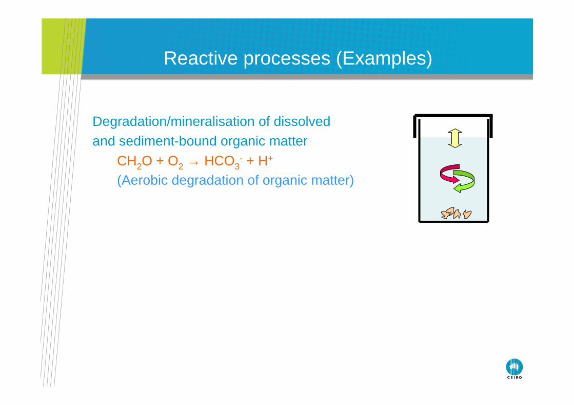
Degradation/mineralisation of dissolved and sediment-bound organic matter

CH2O + O2 → HCO3- + H+

(Aerobic degradation of organic matter)

Reactive processes (Examples)

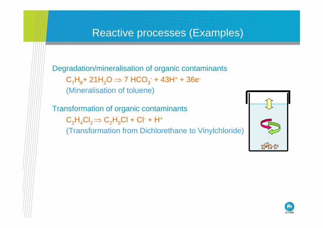
Degradation/mineralisation of organic contaminants

C7H8+ 21H2O ⇒ 7 HCO3- + 43H+ + 36e-

(Mineralisation of toluene)

Transformation of organic contaminants

C2H4Cl2 ⇒ C2H3Cl + Cl- + H+

(Transformation from Dichlorethane to Vinylchloride)

Reactive processes (Examples)

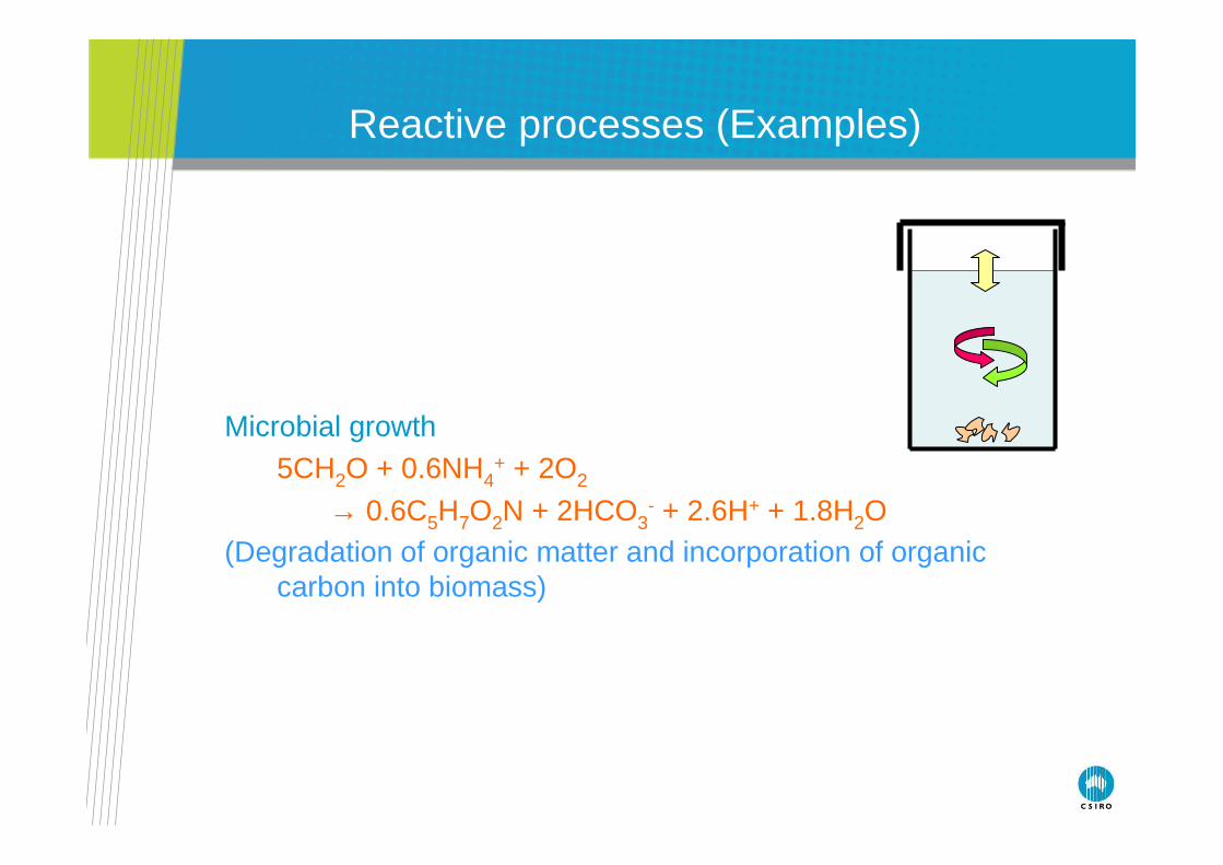
Microbial growth5CH2O + 0.6NH4

+ + 2O2

→ 0.6C5H7O2N + 2HCO3- + 2.6H+ + 1.8H2O

(Degradation of organic matter and incorporation of organiccarbon into biomass)

Reactive processes (Examples)

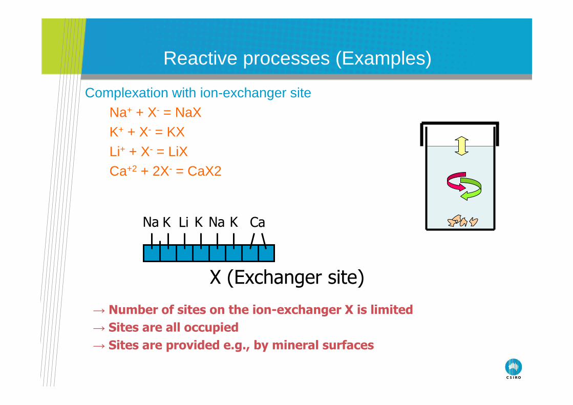
Complexation with ion-exchanger site Na+ + X- = NaXK+ + X- = KXLi+ + X- = LiXCa+2 + 2X- = CaX2

X (Exchanger site)

KK Li K NaNa Ca

→ Number of sites on the ion-exchanger X is limited

→ Sites are all occupied

→ Sites are provided e.g., by mineral surfaces

Reactive processes (Examples)

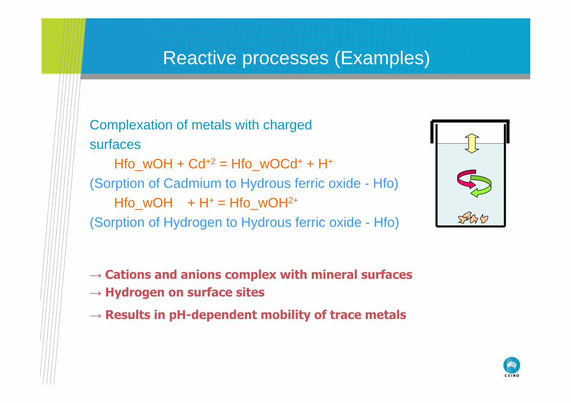
Complexation of metals with charged surfaces

Hfo_wOH + Cd+2 = Hfo_wOCd+ + H+

(Sorption of Cadmium to Hydrous ferric oxide - Hfo)Hfo_wOH + H+ = Hfo_wOH2+

(Sorption of Hydrogen to Hydrous ferric oxide - Hfo)

→ Cations and anions complex with mineral surfaces

→ Hydrogen on surface sites

→ Results in pH-dependent mobility of trace metals

Reactive processes (Examples)

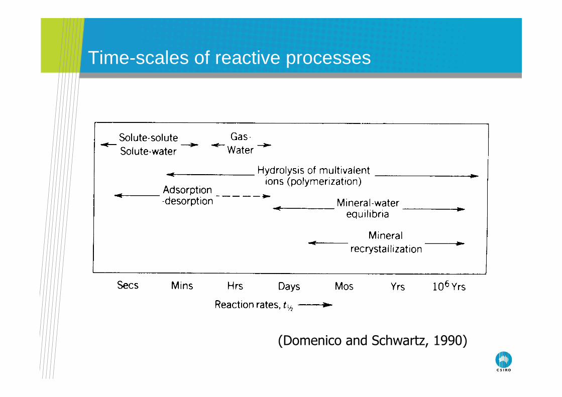
(Domenico and Schwartz, 1990)

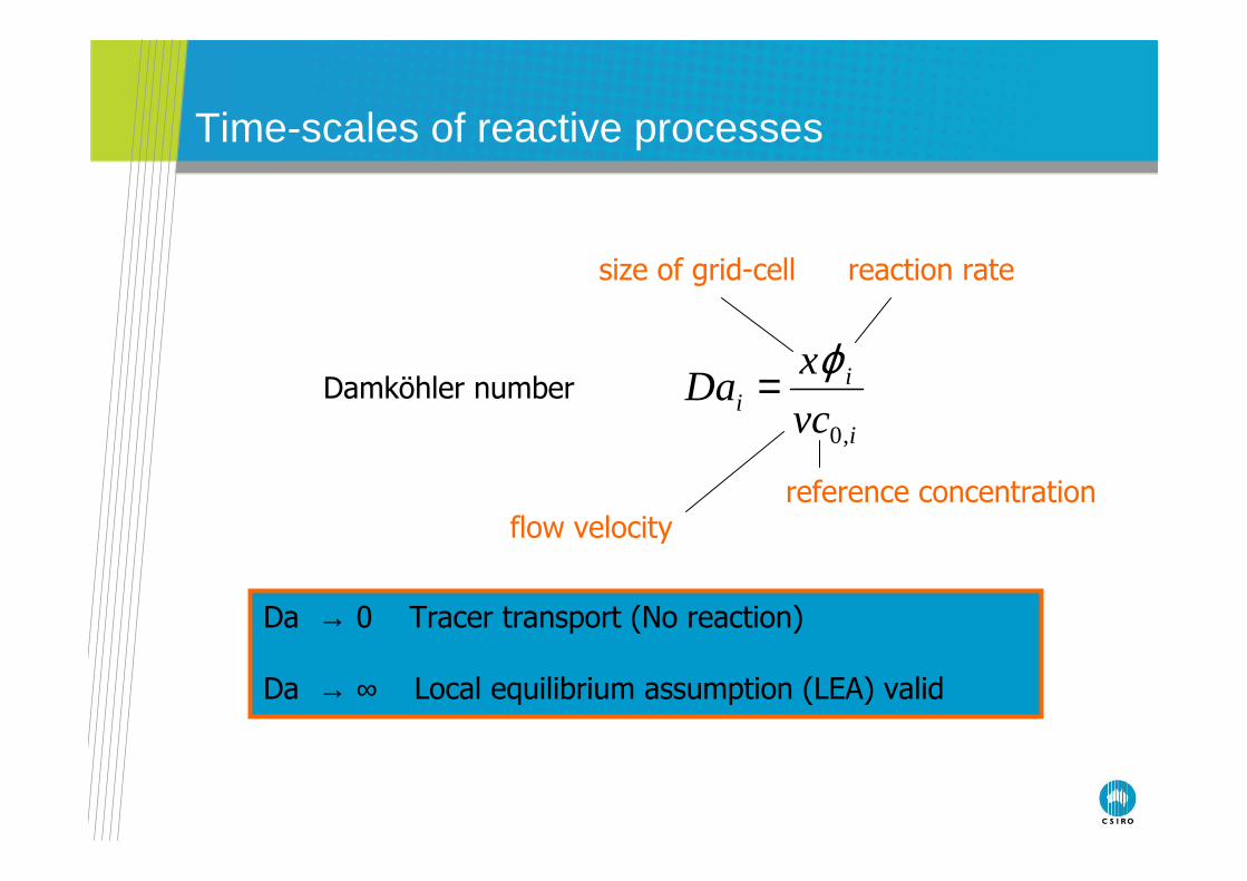
Time-scales of reactive processes

Time-scales of reactive processes

Damköhler number

i

ii vc

xDa

,0

ϕ=

Da → 0 Tracer transport (No reaction)

Da → ∞ Local equilibrium assumption (LEA) valid

size of grid-cell

flow velocity

reaction rate

reference concentration

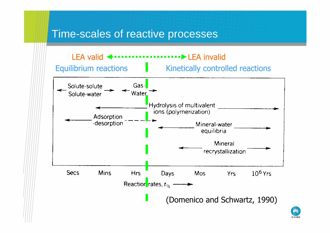
(Domenico and Schwartz, 1990)

LEA invalidLEA valid

Kinetically controlled reactionsEquilibrium reactions

Time-scales of reactive processes

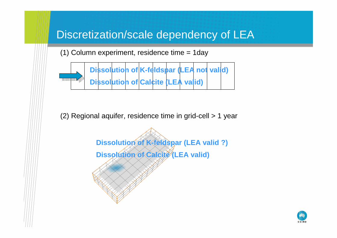
Discretization/scale dependency of LEA

(1) Column experiment, residence time = 1day

Dissolution of K-feldspar (LEA not valid)

Dissolution of Calcite (LEA valid)

(2) Regional aquifer, residence time in grid-cell > 1 year

Dissolution of K-feldspar (LEA valid ?)

Dissolution of Calcite (LEA valid)

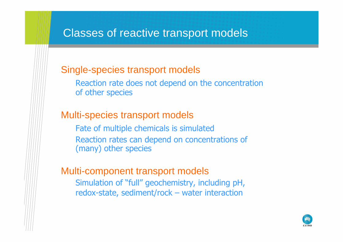
Single-species transport modelsReaction rate does not depend on the concentration of other species

Multi-species transport modelsFate of multiple chemicals is simulated

Reaction rates can depend on concentrations of (many) other species

Multi-component transport modelsSimulation of “full” geochemistry, including pH,

redox-state, sediment/rock – water interaction

Classes of reactive transport models

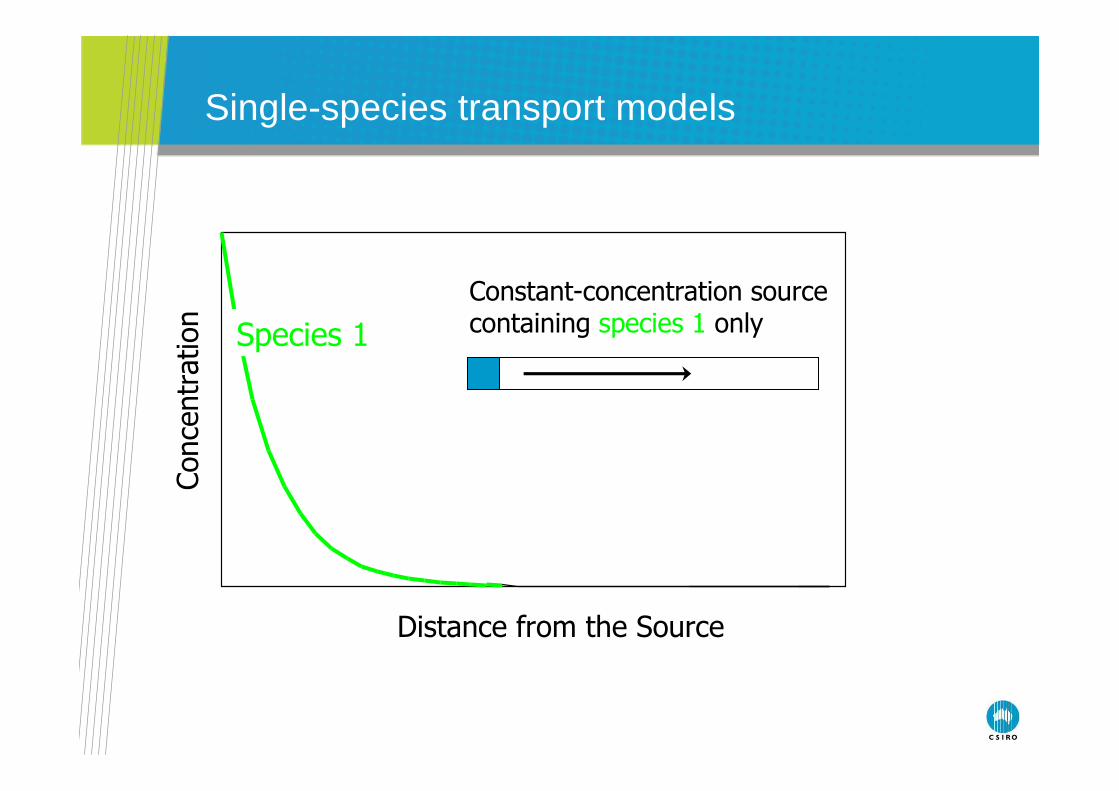
Distance from the Source

Concentration

Species 1

Constant-concentration source containing species 1 only

Single-species transport models

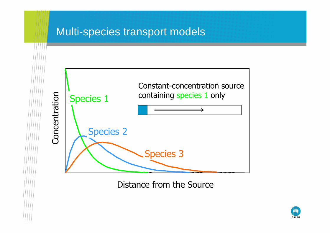
Distance from the Source

Concentration

Species 1

Species 2

Species 3

Constant-concentration source containing species 1 only

Multi-species transport models

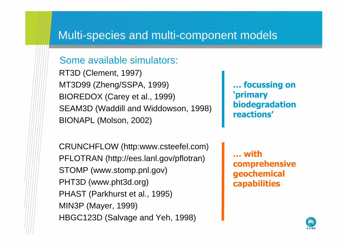
Multi-species and multi-component models

RT3D (Clement, 1997)MT3D99 (Zheng/SSPA, 1999)BIOREDOX (Carey et al., 1999)SEAM3D (Waddill and Widdowson, 1998)BIONAPL (Molson, 2002)

CRUNCHFLOW (http:www.csteefel.com)PFLOTRAN (http://ees.lanl.gov/pflotran)STOMP (www.stomp.pnl.gov) PHT3D (www.pht3d.org)PHAST (Parkhurst et al., 1995)MIN3P (Mayer, 1999)HBGC123D (Salvage and Yeh, 1998)

… focussing on ‘primary biodegradation reactions’

… with comprehensive geochemical capabilities

Some available simulators:

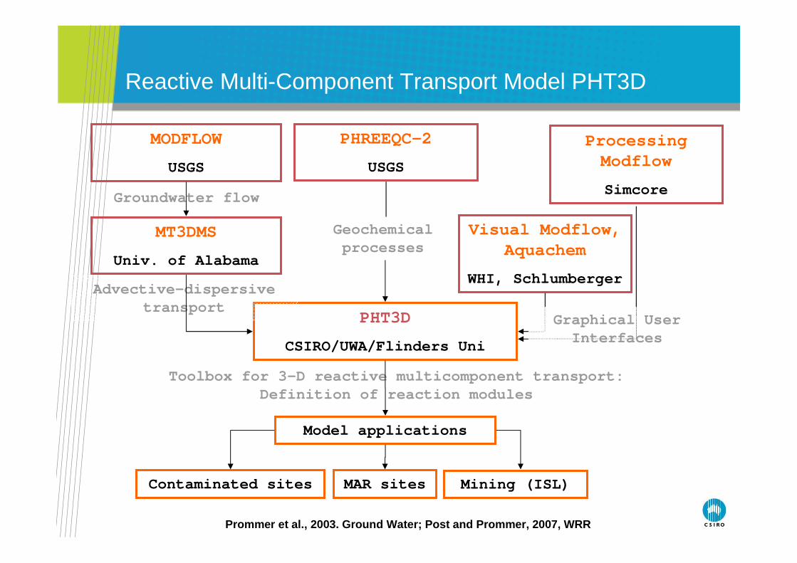
Reactive Multi-Component Transport Model PHT3D

PHT3D

CSIRO/UWA/Flinders Uni

MT3DMS

Univ. of Alabama

PHREEQC-2

USGS

Advective-dispersive transport

MODFLOW

USGS

Groundwater flow

Model applications

Toolbox for 3-D reactive multicomponent transport: Definition of reaction modules

Contaminated sites MAR sites

Visual Modflow, Aquachem

WHI, Schlumberger

Prommer et al., 2003. Ground Water; Post and Prommer, 2007 , WRR

Processing Modflow

Simcore

Graphical User Interfaces

Mining (ISL)

Geochemical processes

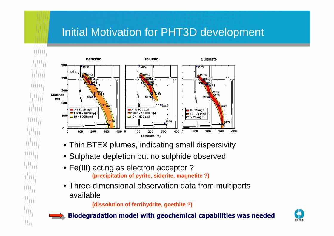
Biodegradation model with geochemical capabilities was needed

Initial Motivation for PHT3D development

• Thin BTEX plumes, indicating small dispersivity• Sulphate depletion but no sulphide observed

• Fe(III) acting as electron acceptor ?(precipitation of pyrite, siderite, magnetite ?)

• Three-dimensional observation data from multiportsavailable

(dissolution of ferrihydrite, goethite ?)

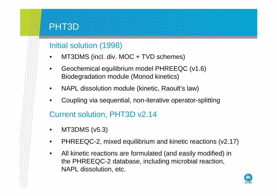
Initial solution (1998)

Current solution, PHT3D v2.14

• MT3DMS (incl. div. MOC + TVD schemes)

• Geochemical equilibrium model PHREEQC (v1.6) Biodegradation module (Monod kinetics)

• NAPL dissolution module (kinetic, Raoult’s law)

• Coupling via sequential, non-iterative operator-splitting

• MT3DMS (v5.3)

• PHREEQC-2, mixed equilibrium and kinetic reactions (v2.17)

• All kinetic reactions are formulated (and easily modified) in the PHREEQC-2 database, including microbial reaction, NAPL dissolution, etc.

PHT3D

PHT3D

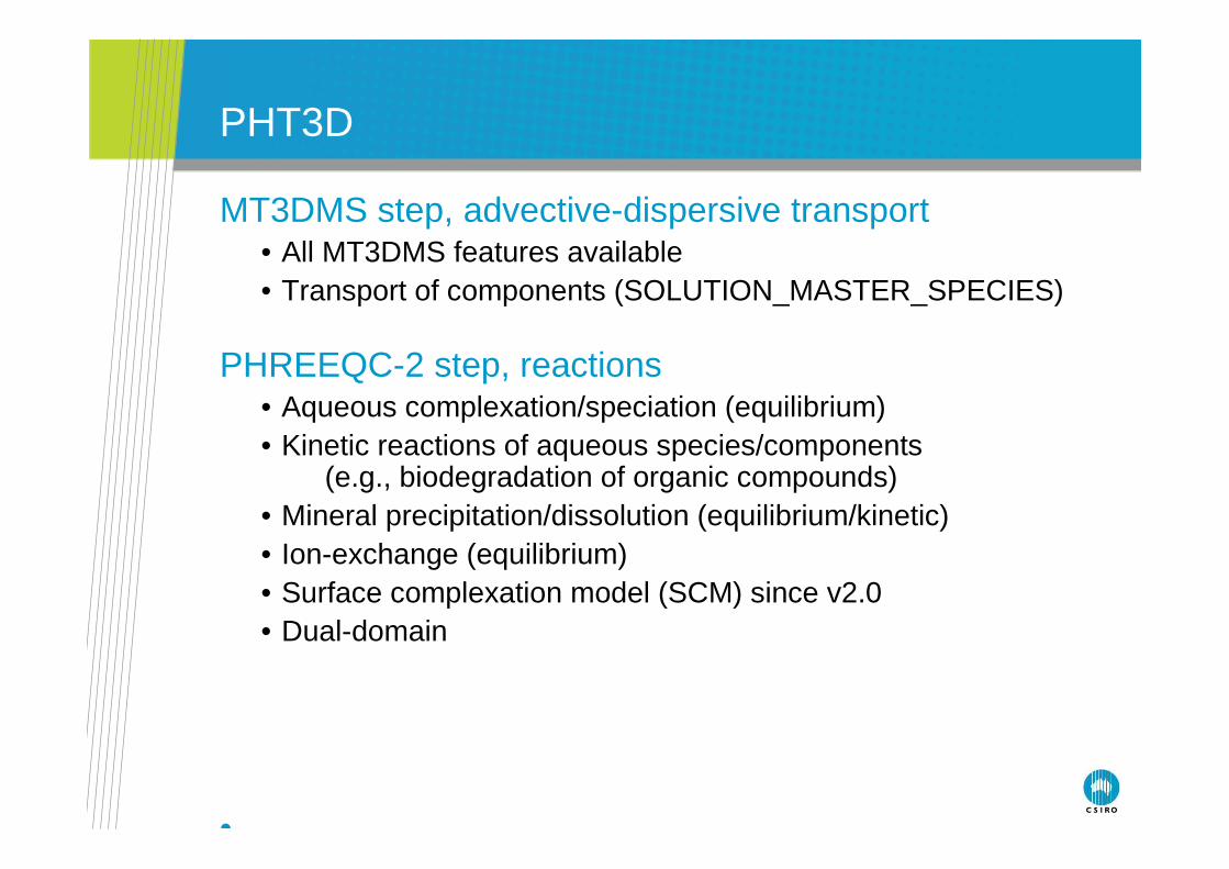
MT3DMS step, advective-dispersive transport • All MT3DMS features available• Transport of components (SOLUTION_MASTER_SPECIES)

PHREEQC-2 step, reactions• Aqueous complexation/speciation (equilibrium)• Kinetic reactions of aqueous species/components

(e.g., biodegradation of organic compounds)• Mineral precipitation/dissolution (equilibrium/kinetic)• Ion-exchange (equilibrium)• Surface complexation model (SCM) since v2.0• Dual-domain

•

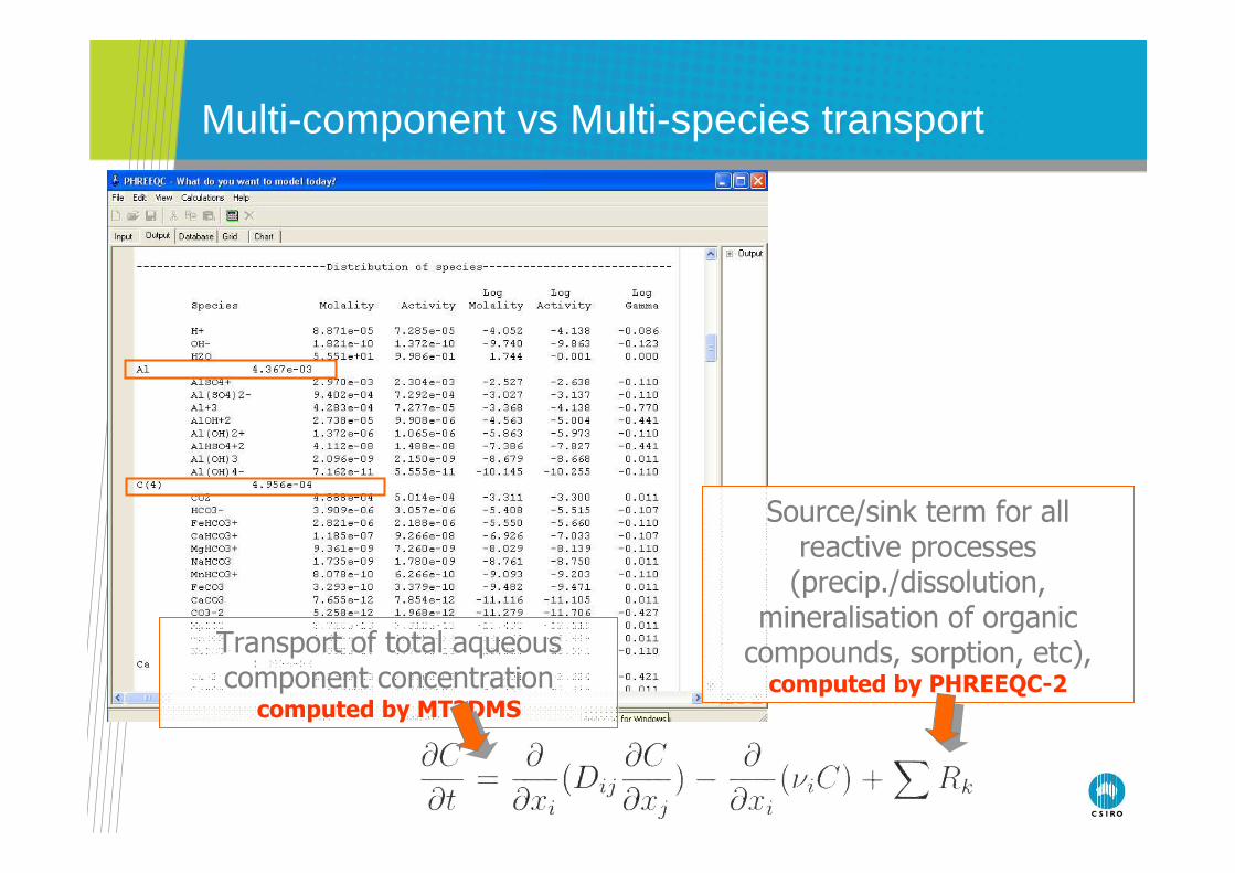
Multi-component vs Multi-species transport

Transport of total aqueous component concentration computed by MT3DMS

Source/sink term for all reactive processes (precip./dissolution,

mineralisation of organic compounds, sorption, etc), computed by PHREEQC-2

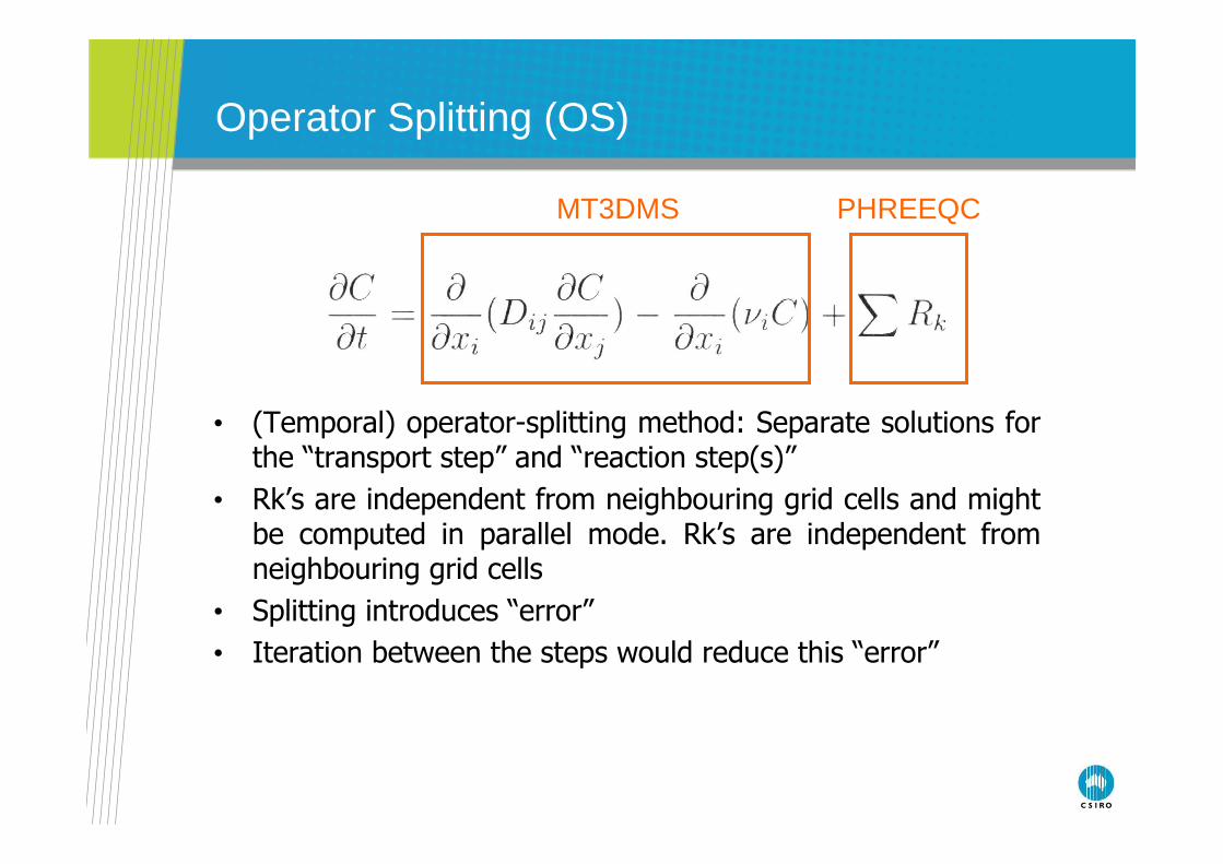
Operator Splitting (OS)

• (Temporal) operator-splitting method: Separate solutions for the “transport step” and “reaction step(s)”

• Rk’s are independent from neighbouring grid cells and might be computed in parallel mode. Rk’s are independent from neighbouring grid cells

• Splitting introduces “error”

• Iteration between the steps would reduce this “error”

MT3DMS PHREEQC

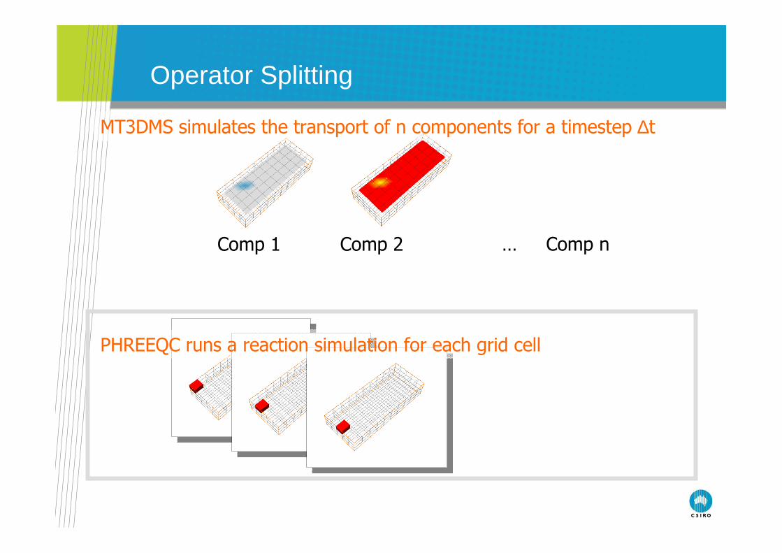
PHREEQC runs a reaction simulation for each grid cell

MT3DMS simulates the transport of n components for a timestep ∆t

Comp 1 Comp 2 … Comp n

Operator Splitting

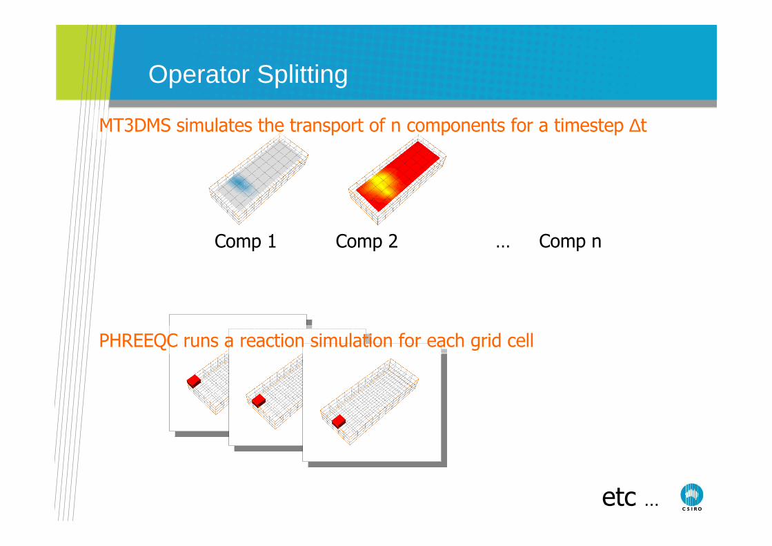
PHREEQC runs a reaction simulation for each grid cell

… Comp n

MT3DMS simulates the transport of n components for a timestep ∆t

Comp 2Comp 1

etc …

Operator Splitting

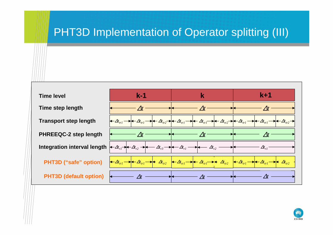
PHT3D Implementation of Operator splitting (III)

Time level k-1 k+1k

∆t ∆tTime step length

Transport step length ∆ttr1 ∆ttr1

∆t

∆ttr2 ∆ttr1 ∆ttr1 ∆ttr2 ∆ttr1 ∆ttr1 ∆ttr2

∆t ∆tPHREEQC-2 step length ∆t

Integration interval length ∆tr3∆tr1 ∆tr2 ∆tr1 ∆tr2 ∆tr1

∆ttr1 ∆ttr1 ∆ttr2 ∆ttr1 ∆ttr1 ∆ttr2 ∆ttr1 ∆ttr1 ∆ttr2PHT3D (“safe” option)

∆t ∆t∆tPHT3D (default option)

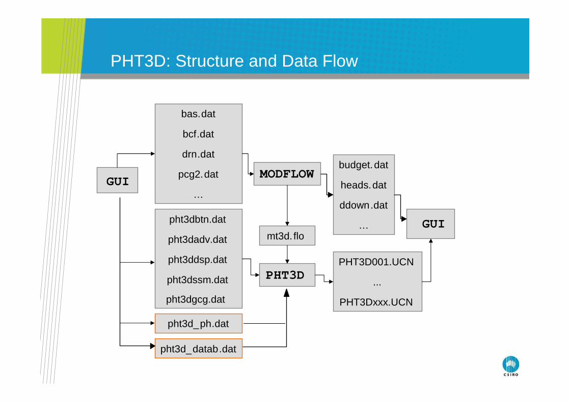
MODFLOW

bas.dat

bcf.dat

drn.dat

pcg2.dat

…

PHT3D

pht3dbtn.dat

pht3dadv.dat

pht3ddsp.dat

pht3dssm.dat

budget.dat

heads.dat

ddown.dat

…mt3d. flo

PHT3D001.UCN

...

PHT3Dxxx.UCN

pht3d_ph.dat

pht3d_datab.dat

GUI

GUI

PHT3D: Structure and Data Flow

pht3dgcg.dat

Mineral Precipitation/Dissolution• Migration of precipitation/dissolution fronts (Engesgaard &

Kipp, 1992) • Acid mine drainage/mineral buffering (Walter et al., 1994)

Ion Exchange• Flushing of a Na-K-NO3 -solution with Ca-Cl2 (Appelo, 1994)• Artificial recharge (Valocchi, 1981)• Anionic tenside injection (Sardin et al., 1986)

Kinetic Reactions• Single-species biodeg./Monod kinetics (Parlange, 1984)• Sequential/parallel decay chain (Sun et al., 1999) • Hydrocarbon degradation using multiple electron acceptors,

RT3D reaction module 3 (Clement, 1997)• Sequential degradation of CHCs,

RT3D reaction module 6 (Clement, 1997)

Verification / benchmark problems

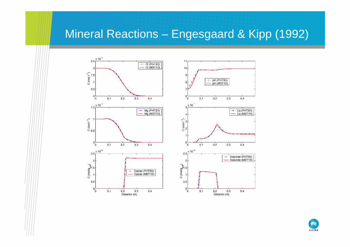
Mineral Reactions – Engesgaard & Kipp (1992)

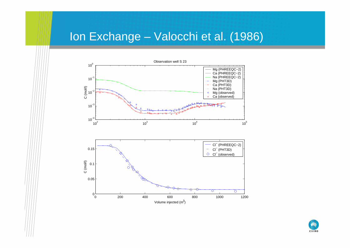
Ion Exchange – Valocchi et al. (1986)

102

103

104

105

10−4

10−3

10−2

10−1

100

Observation well S 23

C (

mol

/l)

Mg (PHREEQC−2)Ca (PHREEQC−2)Na (PHREEQC−2)Mg (PHT3D) Ca (PHT3D) Na (PHT3D) Mg (observed) Ca (observed)

0 200 400 600 800 1000 12000

0.05

0.1

0.15

Volume injected (m3)

C (

mol

/l)

Cl− (PHREEQC−2)Cl− (PHT3D) Cl− (observed)

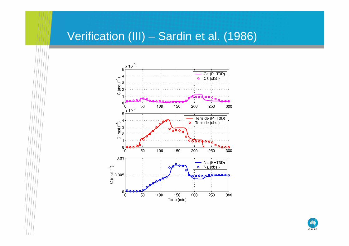
Verification (III) – Sardin et al. (1986)

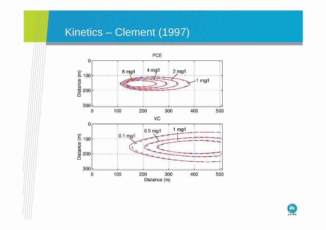
Kinetics – Clement (1997)

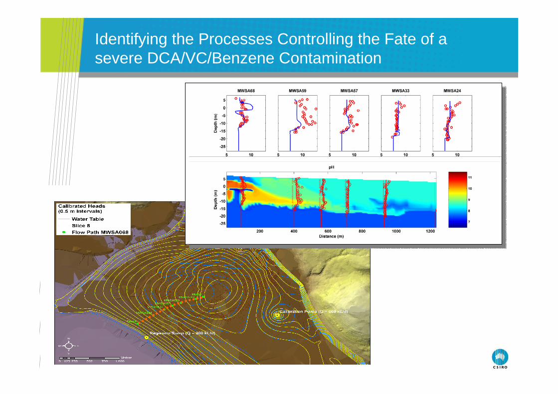
Identifying the Processes Controlling the Fate of a severe DCA/VC/Benzene Contamination

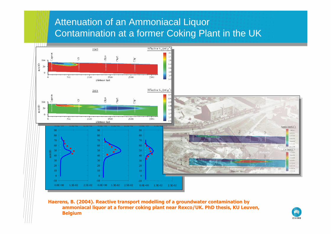
Attenuation of an Ammoniacal Liquor Contamination at a former Coking Plant in the UK

-10

0

10

20

30

40

50

60

70

80

90

0.0E+00 1.3E-02 2.5E-02

0.0E+00 1.3E-02 2.5E-02

-10

0

10

20

30

40

50

60

70

80

90

0.0E+00 1.3E-02 2.5E-02

0.0E+00 1.3E-02 2.5E-02

-10

0

10

20

30

40

50

60

70

80

90

0.0E+00 1.3E-02 2.5E-02

mA

OD

0.0E+00 1.3E-02 2.5E-02

Haerens, B. (2004). Reactive transport modelling of a groundwater contamination by ammoniacal liquor at a former coking plant near Rexco/UK. PhD thesis, KU Leuven, Belgium

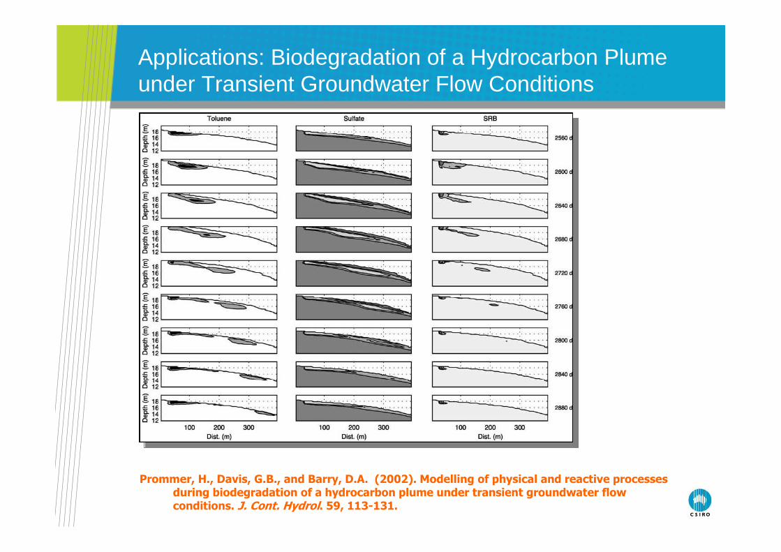
Applications: Biodegradation of a Hydrocarbon Plume under Transient Groundwater Flow Conditions

Prommer, H., Davis, G.B., and Barry, D.A. (2002). Modelling of physical and reactive processes during biodegradation of a hydrocarbon plume under transient groundwater flow conditions. J. Cont. Hydrol. 59, 113-131.

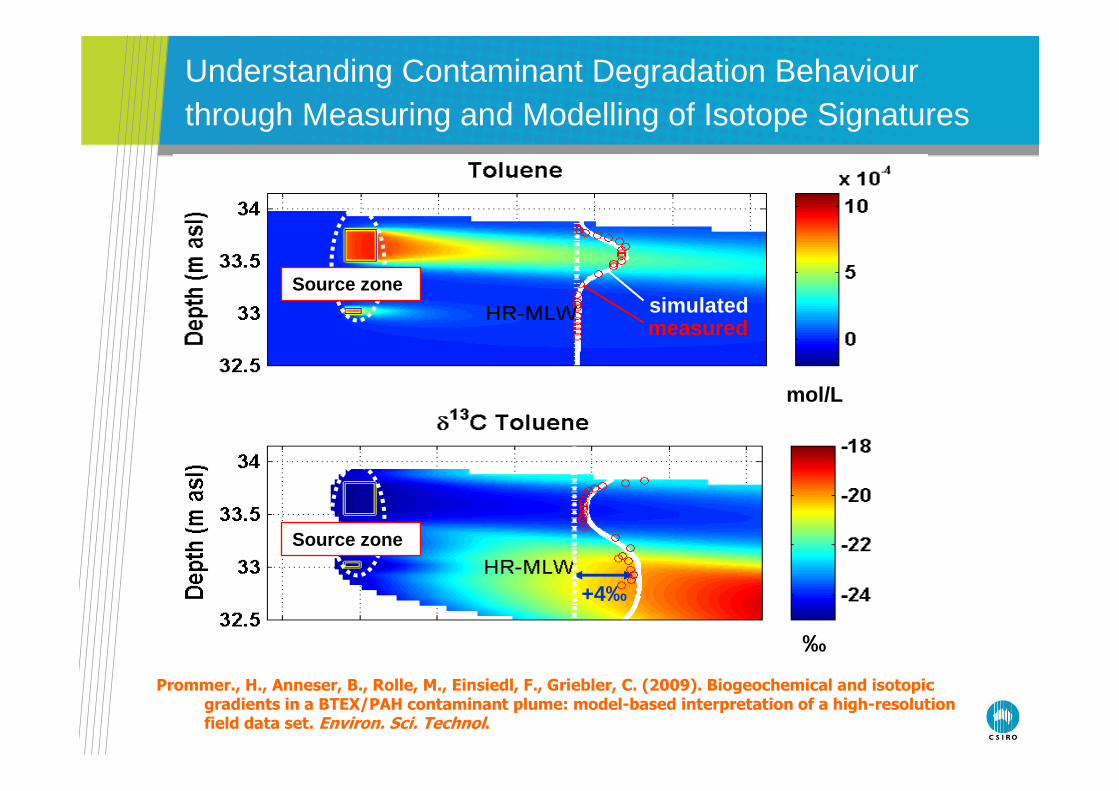
Understanding Contaminant Degradation Behaviourthrough Measuring and Modelling of Isotope Signatures

Prommer., H., Anneser, B., Rolle, M., Einsiedl, F., Griebler, C. (2009). Biogeochemical and isotopic gradients in a BTEX/PAH contaminant plume: model-based interpretation of a high-resolution field data set. Environ. Sci. Technol.

Source zonesimulatedmeasured

mol/L

Source zone

+4‰

‰

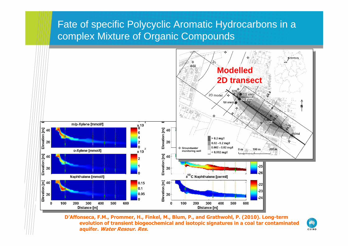
Fate of specific Polycyclic Aromatic Hydrocarbons in a complex Mixture of Organic Compounds

D’Affonseca, F.M., Prommer, H., Finkel, M., Blum, P., and Grathwohl, P. (2010). Long-term evolution of transient biogeochemical and isotopic signatures in a coal tar contaminated aquifer. Water Resour. Res.

Modelled2D transect

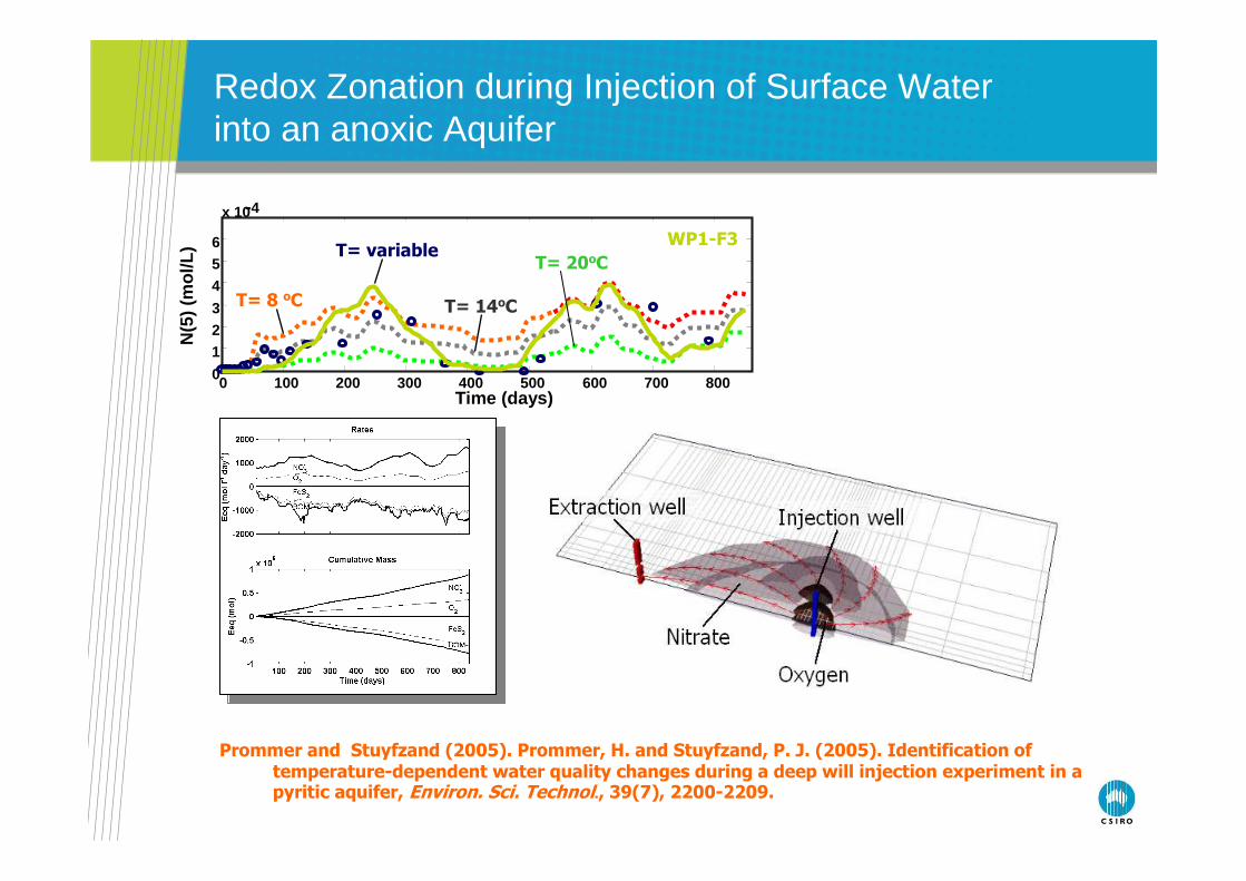
Redox Zonation during Injection of Surface Water into an anoxic Aquifer

0 100 200 300 400 500 600 700 8000

123

456

x 10-4

WP1-F3

N(5

) (m

ol/L

)

Time (days)

T= variable

T= 14oC

T= 20oC

T= 8 oC

Prommer and Stuyfzand (2005). Prommer, H. and Stuyfzand, P. J. (2005). Identification of temperature-dependent water quality changes during a deep will injection experiment in a pyritic aquifer, Environ. Sci. Technol., 39(7), 2200-2209.

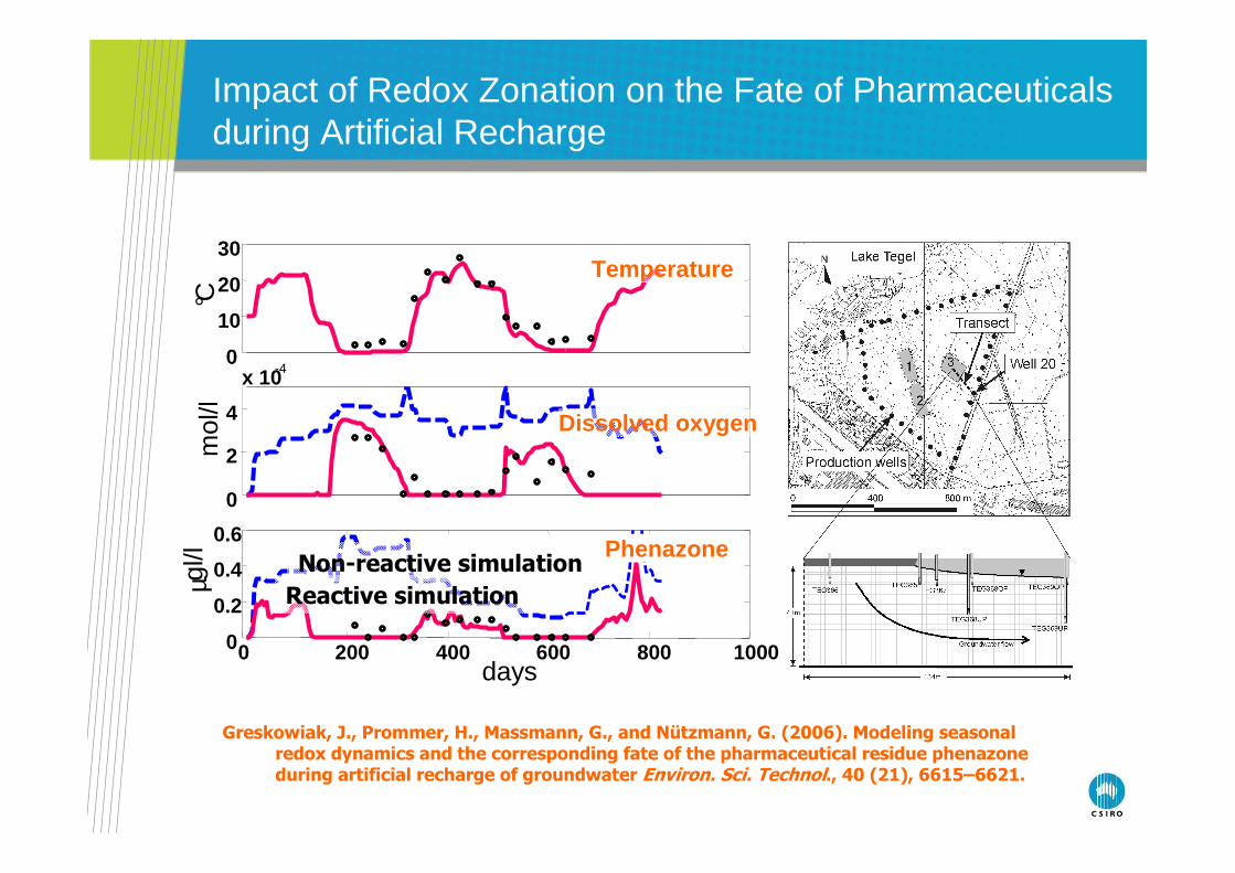
Impact of Redox Zonation on the Fate of Pharmaceuticals during Artificial Recharge

Greskowiak, J., Prommer, H., Massmann, G., and Nützmann, G. (2006). Modeling seasonal redox dynamics and the corresponding fate of the pharmaceutical residue phenazoneduring artificial recharge of groundwater Environ. Sci. Technol., 40 (21), 6615–6621.

0

10

20

30Temperature

°C

0

2

4

x 10-4

Dissolved oxygen

mol

/l

0 200 400 600 800 10000

0.2

0.4

0.6

days

µgl/l Non-reactive simulation

Reactive simulation

Phenazone

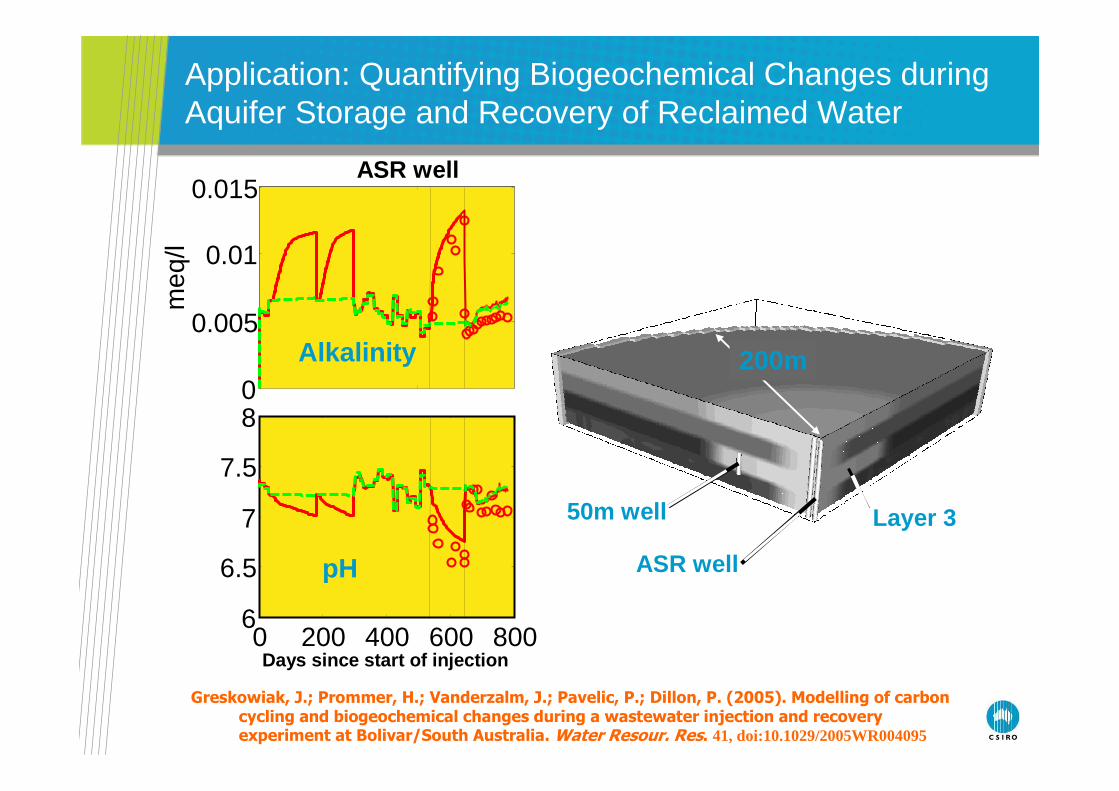
Application: Quantifying Biogeochemical Changes during Aquifer Storage and Recovery of Reclaimed Water

Greskowiak, J.; Prommer, H.; Vanderzalm, J.; Pavelic, P.; Dillon, P. (2005). Modelling of carbon cycling and biogeochemical changes during a wastewater injection and recovery experiment at Bolivar/South Australia. Water Resour. Res. 41, doi:10.1029/2005WR004095

0

0.005

0.01

0.015m

eq/l

ASR well

Alkalinity

0 200 400 600 8006

6.5

7

7.5

8

Days since start of injection

pH

Layer 350m well

ASR well

200m

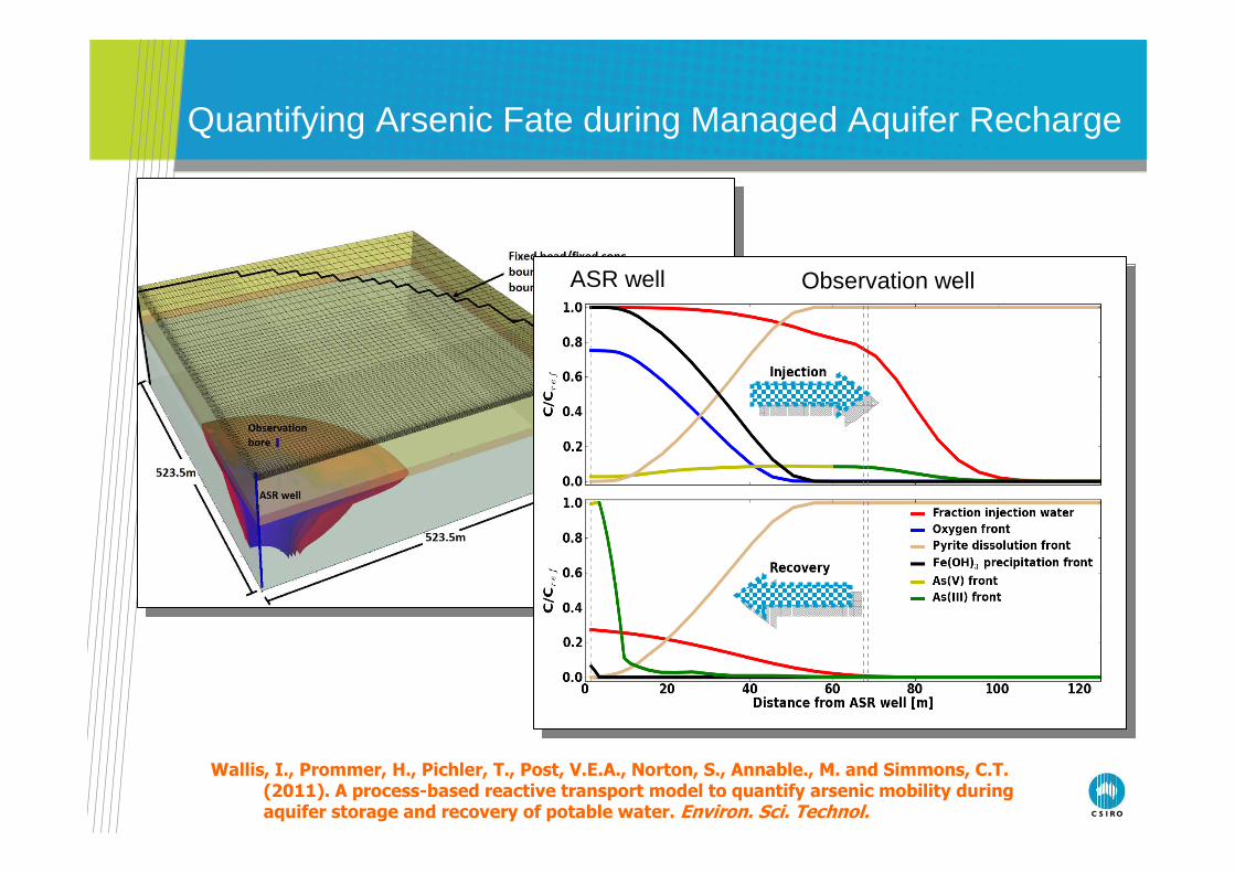
Quantifying Arsenic Fate during Managed Aquifer Recharge

Wallis, I., Prommer, H., Pichler, T., Post, V.E.A., Norton, S., Annable., M. and Simmons, C.T. (2011). A process-based reactive transport model to quantify arsenic mobility during aquifer storage and recovery of potable water. Environ. Sci. Technol.

ASR well Observation well

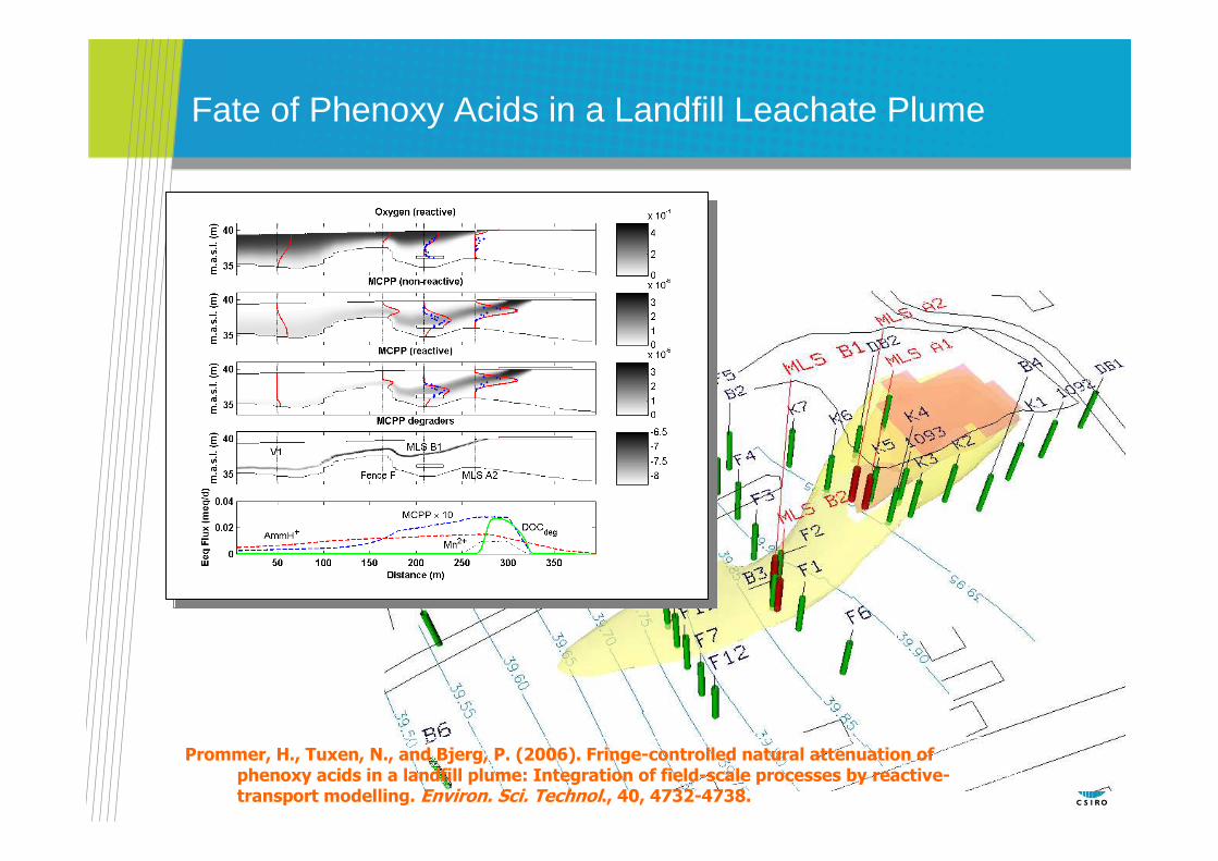
Fate of Phenoxy Acids in a Landfill Leachate Plume

Prommer, H., Tuxen, N., and Bjerg, P. (2006). Fringe-controlled natural attenuation of phenoxy acids in a landfill plume: Integration of field-scale processes by reactive-transport modelling. Environ. Sci. Technol., 40, 4732-4738.

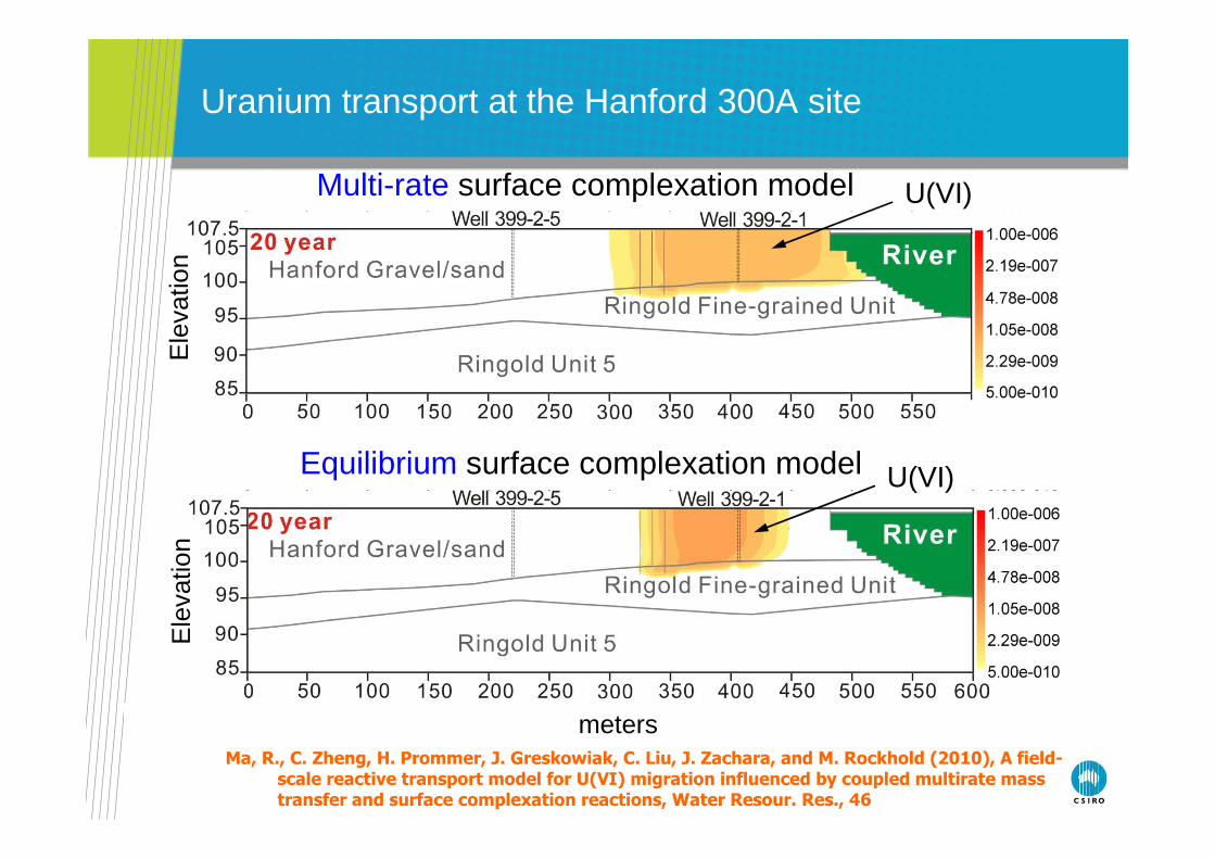
Uranium transport at the Hanford 300A site

meters

Multi-rate surface complexation model

Equilibrium surface complexation model

U(VI)

U(VI)

Ele

vatio

nE

leva

tion

Ma, R., C. Zheng, H. Prommer, J. Greskowiak, C. Liu, J. Zachara, and M. Rockhold (2010), A field-scale reactive transport model for U(VI) migration influenced by coupled multirate mass transfer and surface complexation reactions, Water Resour. Res., 46

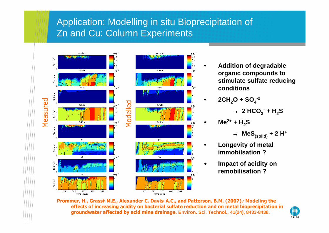
Application: Modelling in situ Bioprecipitation of Zn and Cu: Column Experiments

Prommer, H., Grassi, M.E., Alexander C. Davis, A.C., and Patterson, B.M. (2007)., Modeling the effects of increasing acidity on bacterial sulfate reduction and on metal bioprecipitation in groundwater affected by acid mine drainage. Environ. Sci. Technol., 41(24), 8433-8438.

• Addition of degradable organic compounds to stimulate sulfate reducing conditions

• 2CH2O + SO4-2

→→→→ 2 HCO3- + H2S

• Me2+ + H2S

→→→→ MeS(solid) + 2 H+

• Longevity of metal immobilsation ?

• Impact of acidity on remobilisation ?

Measu

red

Modelled

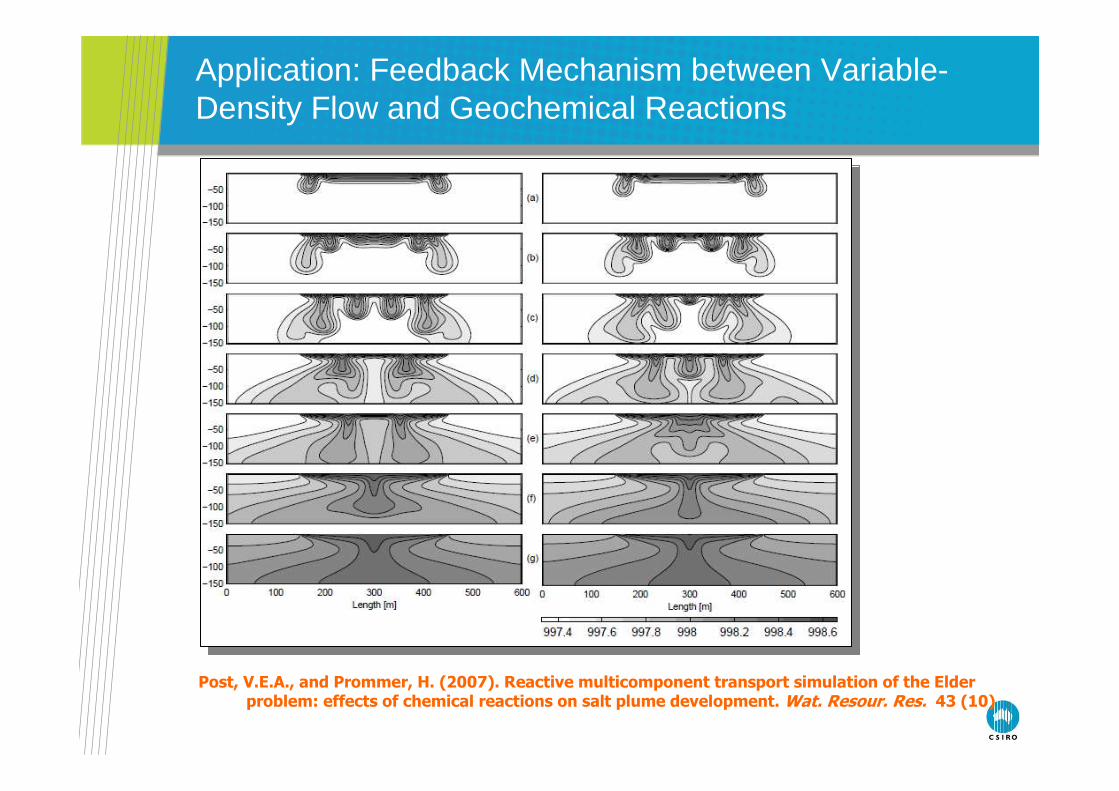
Application: Feedback Mechanism between Variable-Density Flow and Geochemical Reactions

Post, V.E.A., and Prommer, H. (2007). Reactive multicomponent transport simulation of the Elder problem: effects of chemical reactions on salt plume development. Wat. Resour. Res. 43 (10)

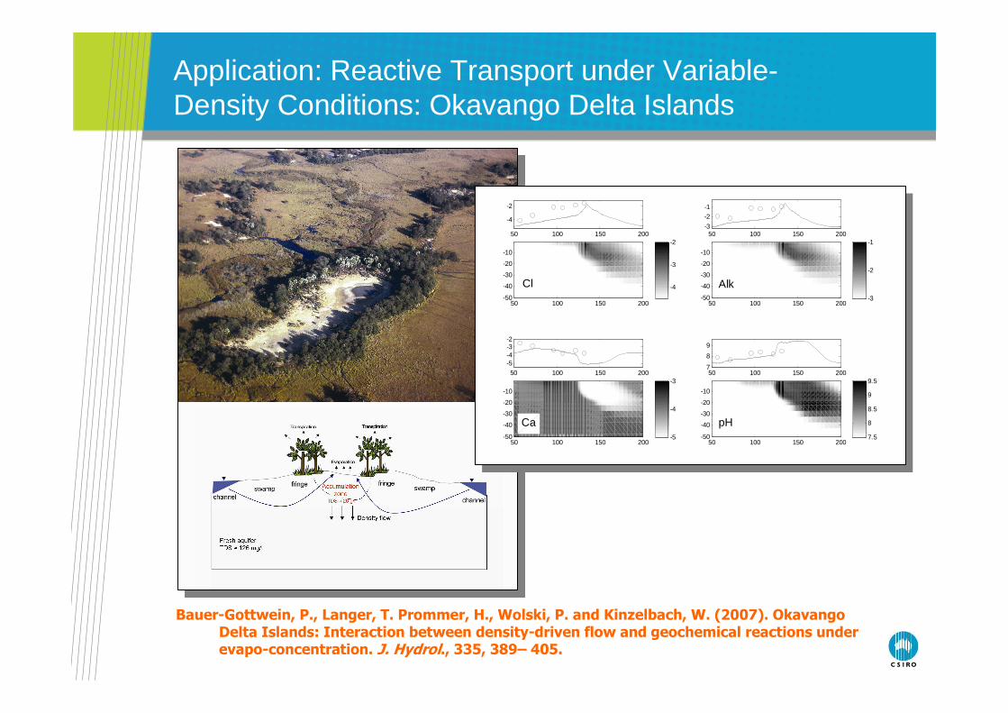
Bauer-Gottwein, P., Langer, T. Prommer, H., Wolski, P. and Kinzelbach, W. (2007). Okavango Delta Islands: Interaction between density-driven flow and geochemical reactions under evapo-concentration. J. Hydrol., 335, 389– 405.

Application: Reactive Transport under Variable-Density Conditions: Okavango Delta Islands

50 100 150 200-50

-40

-30

-20

-10

50 100 150 200-50

-40

-30

-20

-10

50 100 150 200-50

-40

-30

-20

-10

50 100 150 200-50

-40

-30

-20

-10

-4

-3

-2

-3

-2

-1

-5

-4

-3

7.5

8

8.5

9

9.5

50 100 150 200

-4

-2

50 100 150 200-3

-2

-1

50 100 150 200

-5-4-3-2

50 100 150 2007

8

9

Cl

pHCa

Alk

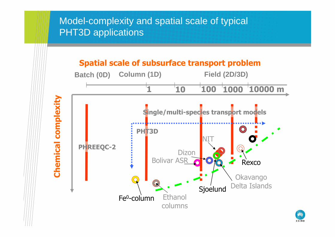
Spatial scale of subsurface transport problemChemical complexity

Batch (0D) Column (1D) Field (2D/3D)

1 10 100 1000 10000 m

PHT3D

Rexco

Sjoelund

Fe0-column

Model-complexity and spatial scale of typical PHT3D applications

Ethanol columns

Dizon

NIT

Okavango Delta Islands

Bolivar ASR

Single/multi-species transport models

PHREEQC-2

Warning:Reactive transport ≠ regional MODFLOW model + reactions

• Vertical chemical gradients may be much more significant than lateral chemical gradients

• Vertical grid resolution of flow models is often insufficient toresolve these vertical chemical gradients – especially were vertical transverse mixing controls the progress of reactions

• Even pefectly calibrated flow models may not predict transport behaviour very well – chemical data needed as additional constraints

• (Desktop) computational power is only slowly sufficient to allow 3D (high resolution) models

Warning:Reactive transport ≠ regional MODFLOW model + reactions

Be smart• Think hard(er) about the combined conceptual

hydrogeological + chemical model• Is perhaps a 2D vertical transect sufficient to address the

reactive transport problem ?• Is a 3D reactive transport model for a subregion of the flow

model sufficent ?• Is the problem symmetric ? (ASR, Deepwell injection, ....)• Can a rough calibration be carried out on a less refined grid

and grid resolution successively increased ?

From simple to complex• Test + debug chemical reactions (e.g, rate expressions for

kinetics) in 0D (PHREEQC batch mode).• Build a mickey mouse model with reactions (1D, 2D) and

debug problems + get a feel for the processes

Initial and boundary conditions• Formulation of initial and boundary conditions is similar to

MT3DMS. • Note, that the same type of boundary condition applies to all

components/compounds.• Water chemistry (solution composition) must be defined for all

boundaries with a positive flux into the model, otherwise “de-ionized” water is added to the domain (C = 0 for all species)

• Solution compositions at boundaries must be charge-balanced and (depending on the conceptual model) be pre-equilibrated with the minerals

• Initial solution composition(s) should be charge-balanced and pre-equilibrated with the mineral assemblage etc.

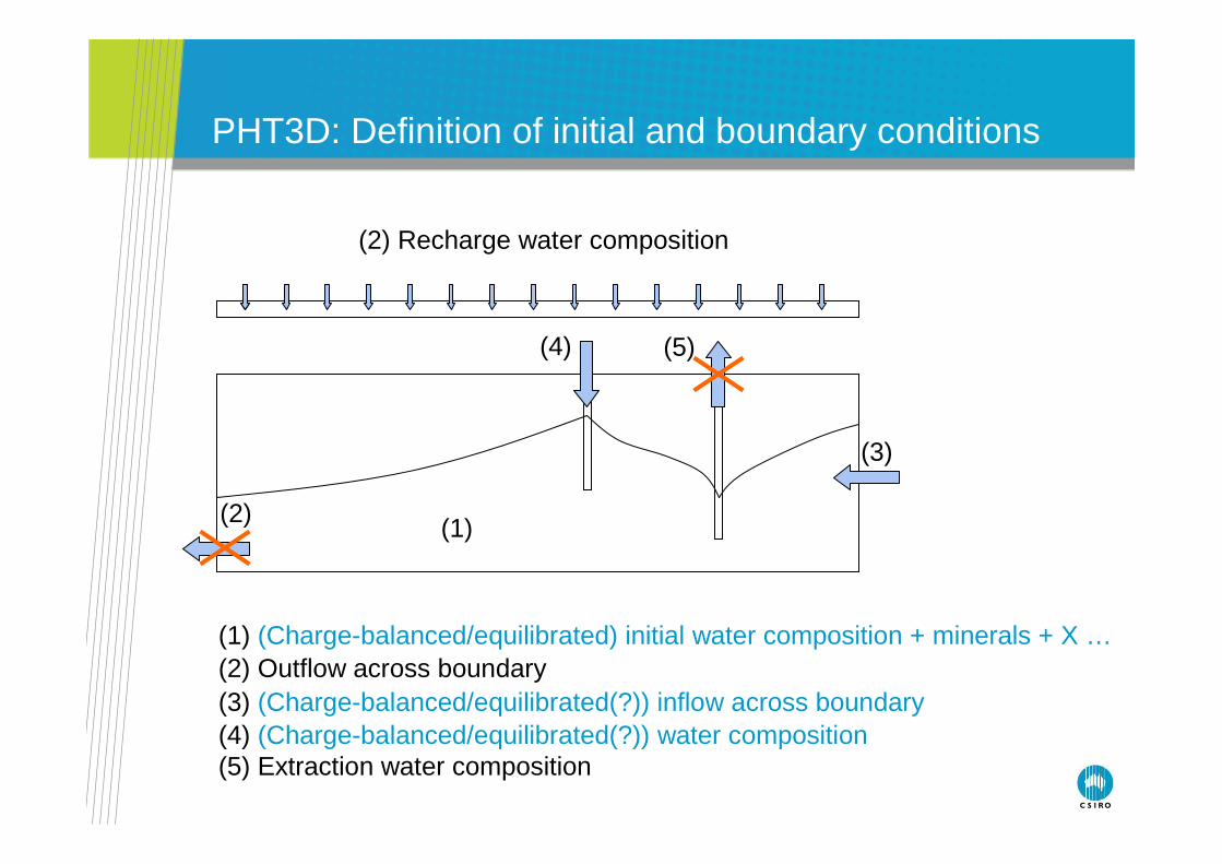
PHT3D: Definition of initial and boundary conditions

(2) Recharge water composition

(3)

(2) (1)

(4) (Charge-balanced/equilibrated(?)) water composition

(4) (5)

(3) (Charge-balanced/equilibrated(?)) inflow across boundary

(1) (Charge-balanced/equilibrated) initial water composition + minerals + X …(2) Outflow across boundary

(5) Extraction water composition

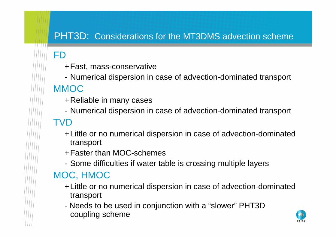
FD+Fast, mass-conservative- Numerical dispersion in case of advection-dominated transport

MMOC+Reliable in many cases- Numerical dispersion in case of advection-dominated transport

TVD+Little or no numerical dispersion in case of advection-dominated

transport+Faster than MOC-schemes - Some difficulties if water table is crossing multiple layers

MOC, HMOC+Little or no numerical dispersion in case of advection-dominated

transport- Needs to be used in conjunction with a “slower” PHT3D

coupling scheme

PHT3D: Considerations for the MT3DMS advection scheme

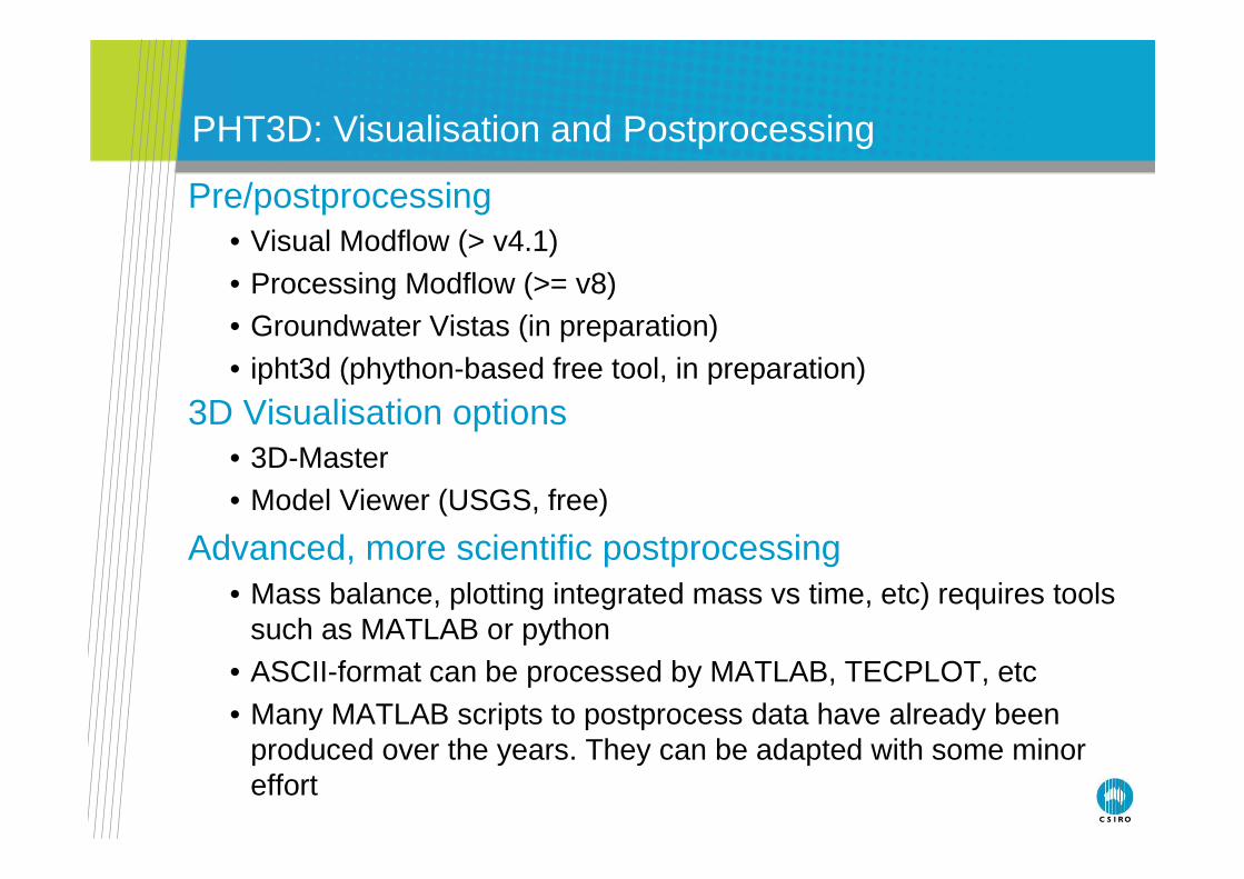
PHT3D: Visualisation and Postprocessing

Pre/postprocessing• Visual Modflow (> v4.1) • Processing Modflow (>= v8)• Groundwater Vistas (in preparation)• ipht3d (phython-based free tool, in preparation)

3D Visualisation options• 3D-Master• Model Viewer (USGS, free)

Advanced, more scientific postprocessing• Mass balance, plotting integrated mass vs time, etc) requires tools

such as MATLAB or python• ASCII-format can be processed by MATLAB, TECPLOT, etc• Many MATLAB scripts to postprocess data have already been

produced over the years. They can be adapted with some minor effort

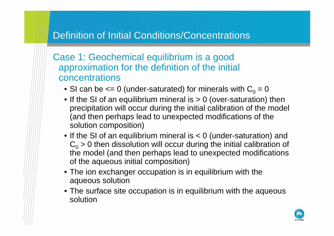
Definition of Initial Conditions/Concentrations

Case 1: Geochemical equilibrium is a good approximation for the definition of the initial concentrations

• SI can be <= 0 (under-saturated) for minerals with C0 = 0 • If the SI of an equilibrium mineral is > 0 (over-saturation) then

precipitation will occur during the initial calibration of the model (and then perhaps lead to unexpected modifications of the solution composition)

• If the SI of an equilibrium mineral is < 0 (under-saturation) and C0 > 0 then dissolution will occur during the initial calibration of the model (and then perhaps lead to unexpected modifications of the aqueous initial composition)

• The ion exchanger occupation is in equilibrium with the aqueous solution

• The surface site occupation is in equilibrium with the aqueous solution

Definition of Initial Conditions/Concentrations

Case 2: Quasi-dynamic equilibrium • Slow, kinetically controlled weathering reactions … SI does not

or only very slowly reach 0 within the model domain …. • Example: Kinetically controlled DOC or SOM degradation or

other processes cause a redox zonation within aquifer

→ Apply spin-up period

... e.g., model domain completely flushed once