Embed Size (px)
Citation preview
Machine Learning Classical Conditioning Synaptic Plasticity
Dynamic Prog.(Bellman Eq.)
REINFORCEMENT LEARNING UN-SUPERVISED LEARNINGexample based correlation based
d-Rule
Monte CarloControl
Q-Learning
TD( )often =0
ll
TD(1) TD(0)
Rescorla/Wagner
Neur.TD-Models(“Critic”)
Neur.TD-formalism
DifferentialHebb-Rule
(”fast”)
STDP-Modelsbiophysical & network
EVALUATIVE FEEDBACK (Rewards)
NON-EVALUATIVE FEEDBACK (Correlations)
SARSA
Correlationbased Control
(non-evaluative)
ISO-Learning
ISO-Modelof STDP
Actor/Critictechnical & Basal Gangl.
Eligibility Traces
Hebb-Rule
DifferentialHebb-Rule
(”slow”)
supervised L.
Anticipatory Control of Actions and Prediction of Values Correlation of Signals
=
=
=
Neuronal Reward Systems(Basal Ganglia)
Biophys. of Syn. PlasticityDopamine Glutamate
STDP
LTP(LTD=anti)
ISO-Control
Overview over different methods
You are here !
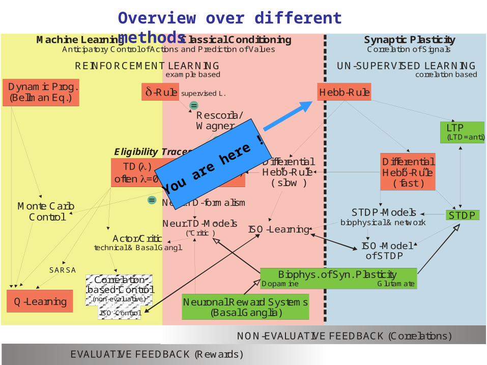
Hebbian learning
AB
A
B
t
When an axon of cell A excites cell B and repeatedly or persistently takes part in firing it, some growth processes or metabolic change takes place in one or both cells so that A‘s efficiency ... is increased.
Donald Hebb (1949)
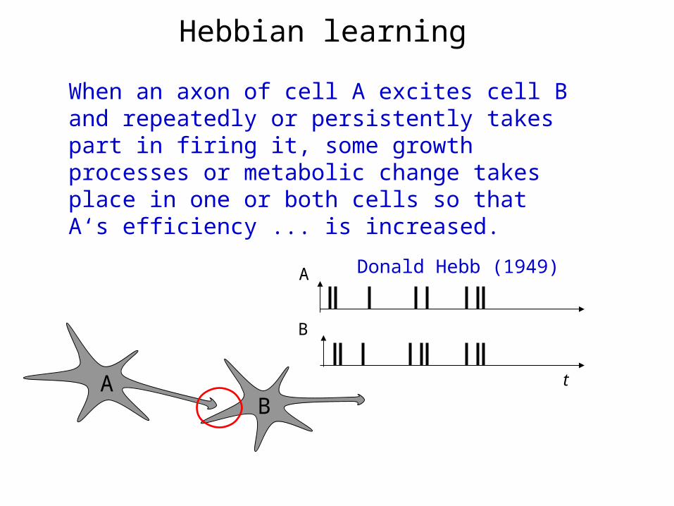
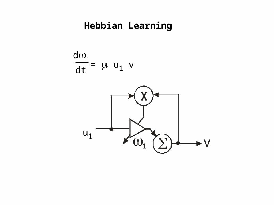
Hebbian Learning
…Basic Hebb-Rule:
…correlates inputs with outputs by the…
= v u1 << 1d
dt
vu1
Vector Notation following Dayan and Abbott:
Cell Activity: v = w . u
This is a dot product, where w is a weight vector and uthe input vector. Strictly we need to assume that weightchanges are slow, otherwise this turns into a differential eq.
1
X
x1
vS
= u1 vd
dt
Hebbian Learning
u1
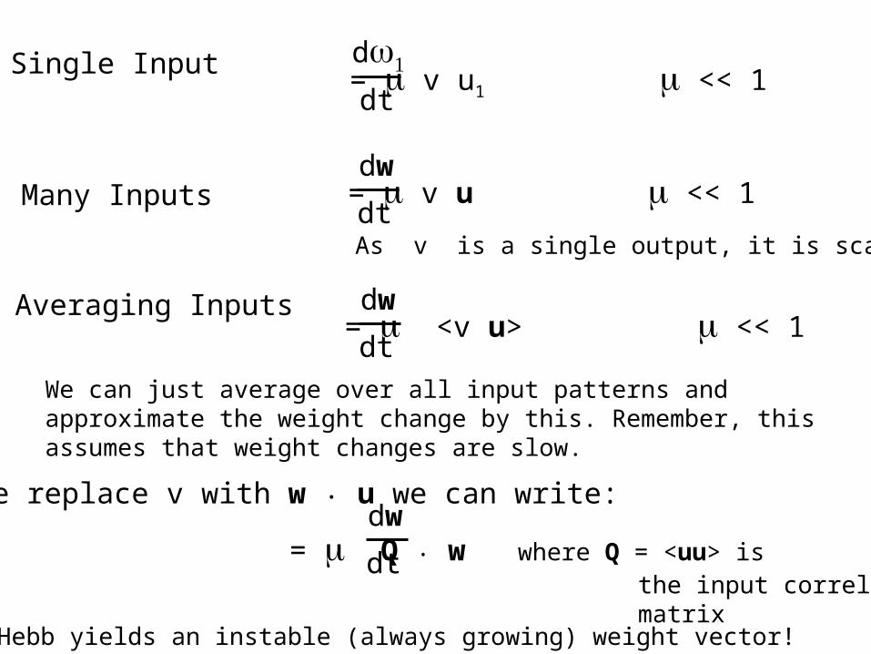
= v u1 << 1d
dtSingle Input
= v u << 1dw
dtMany Inputs
As v is a single output, it is scalar.
Averaging Inputs= <v u> << 1
dw
dt
We can just average over all input patterns and approximate the weight change by this. Remember, this assumes that weight changes are slow.
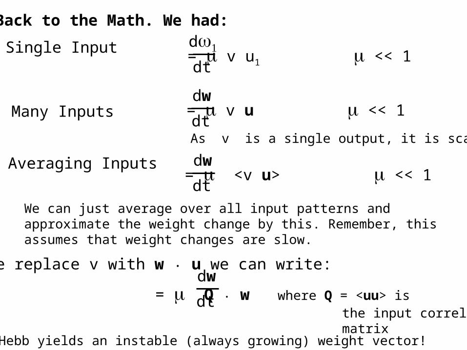
If we replace v with w . u we can write:
= Q . w where Q = <uu> is the input correlation matrix
dw
dt
Note: Hebb yields an instable (always growing) weight vector!
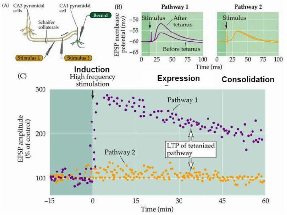
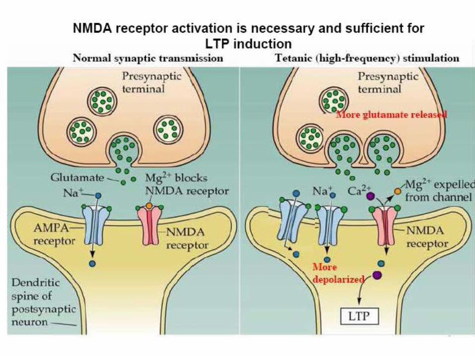
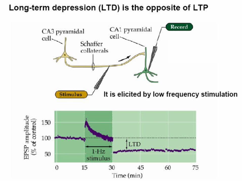
Synaptic plasticity evoked artificially
Examples of Long term potentiation (LTP)and long term depression (LTD).
LTP First demonstrated by Bliss and Lomo in 1973. Since then induced in many different ways, usually in slice.
LTD, robustly shown by Dudek and Bear in 1992, in Hippocampal slice.
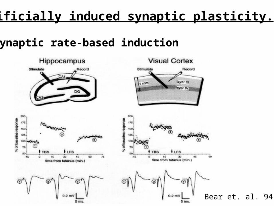
Artificially induced synaptic plasticity.
Presynaptic rate-based induction
Bear et. al. 94
Feldman, 2000
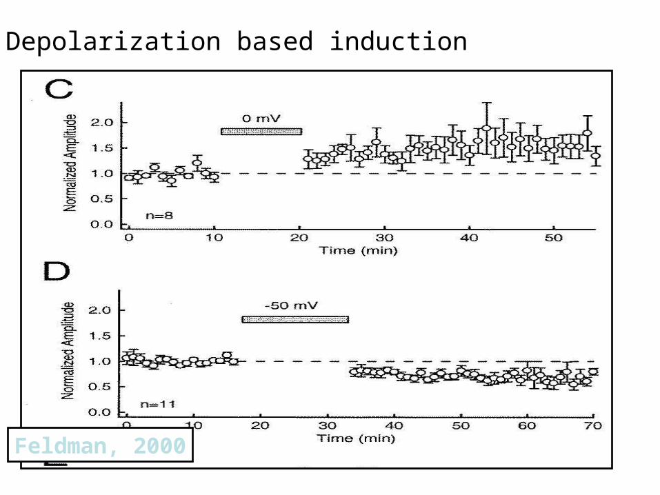
Depolarization based induction
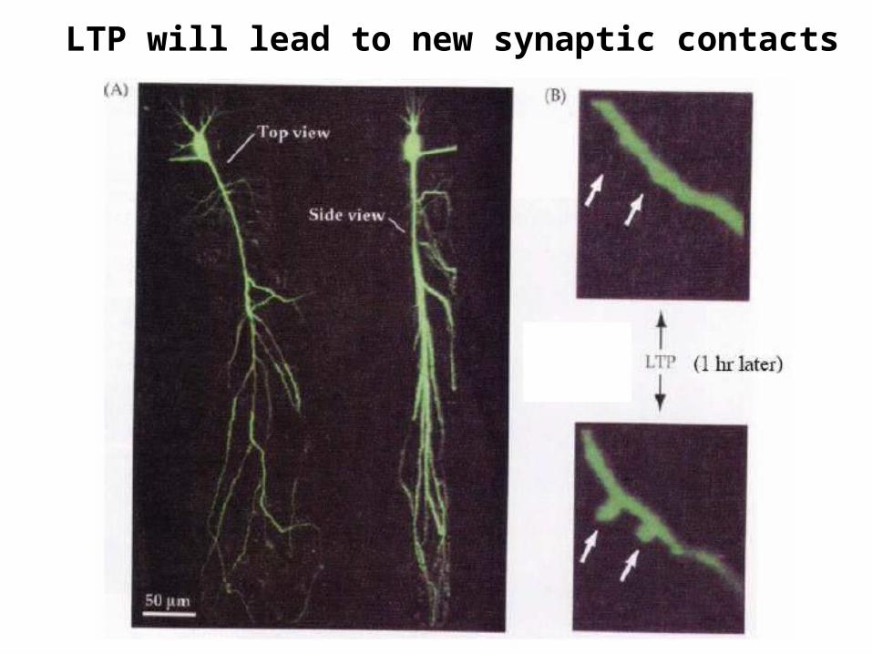
LTP will lead to new synaptic contacts
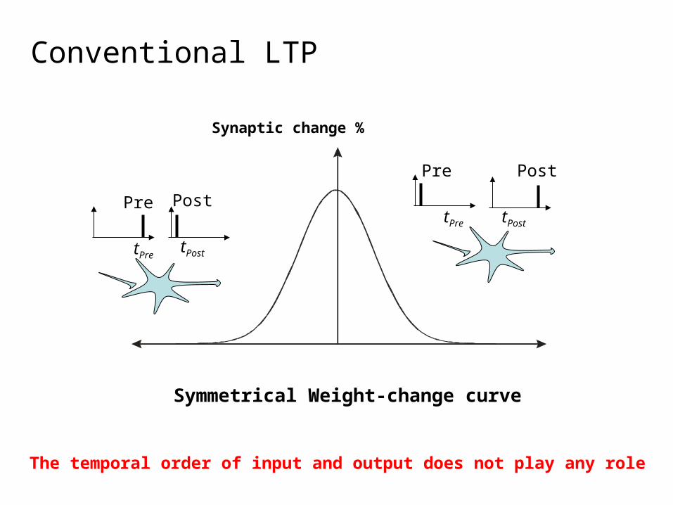
Conventional LTP
Symmetrical Weight-change curve
Pre
tPre
Post
tPost
Synaptic change %
Pre
tPre
Post
tPost
The temporal order of input and output does not play any role
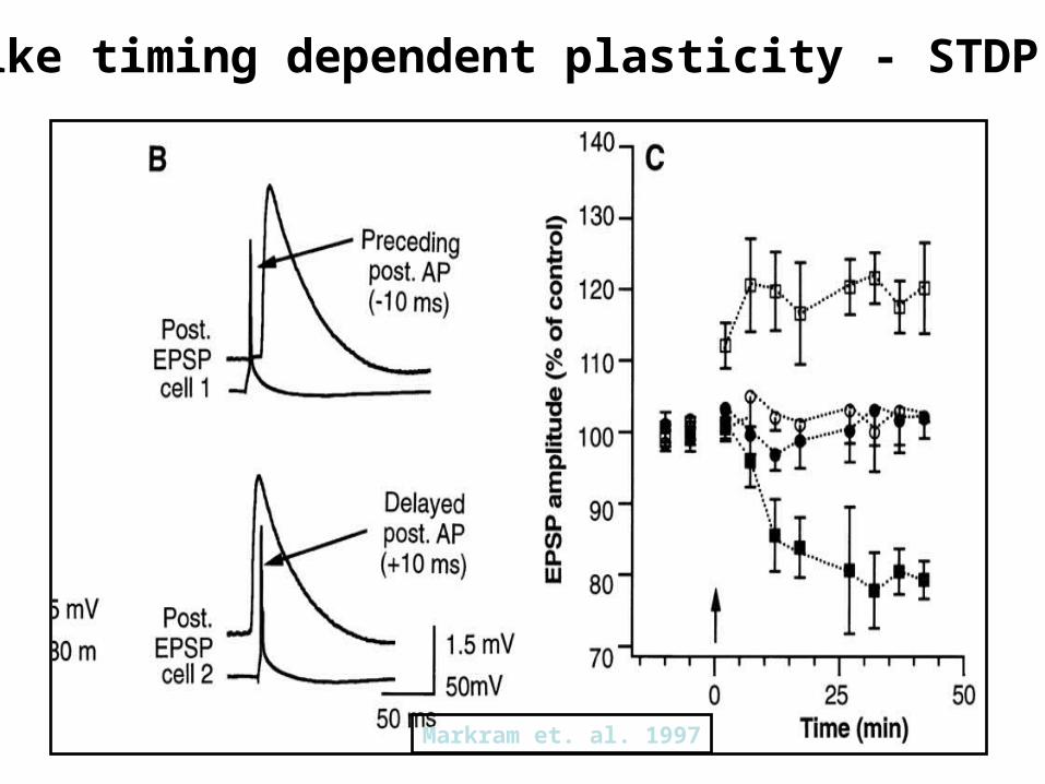
Spike timing dependent plasticity - STDP
Markram et. al. 1997
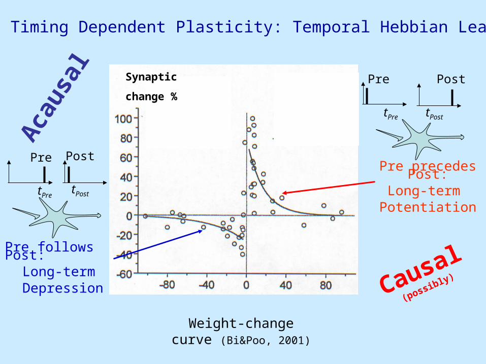
Pre follows Post:Long-term Depression
Pre
tPre
Post
tPost
Synaptic
change %
Spike Timing Dependent Plasticity: Temporal Hebbian Learning
Weight-change curve (Bi&Poo, 2001)
Pre
tPre
Post
tPost
Pre precedes Post:Long-term Potentiation
Aca
usal
Causal
(possibly)
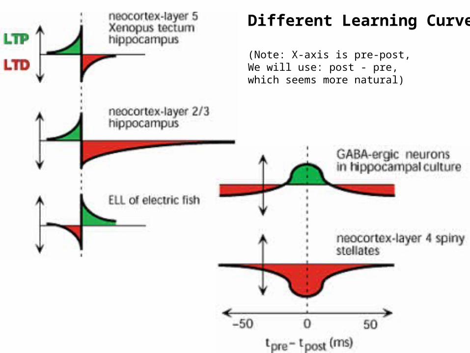
Different Learning Curves
(Note: X-axis is pre-post,We will use: post - pre,which seems more natural)

But how do we know that “synaptic plasticity” as observed on the cellular level has any connection to learning and memory?
What types of criterions can we use to answer this question?
At this level we know much about the cellular and molecular basis of synaptic plasticity.
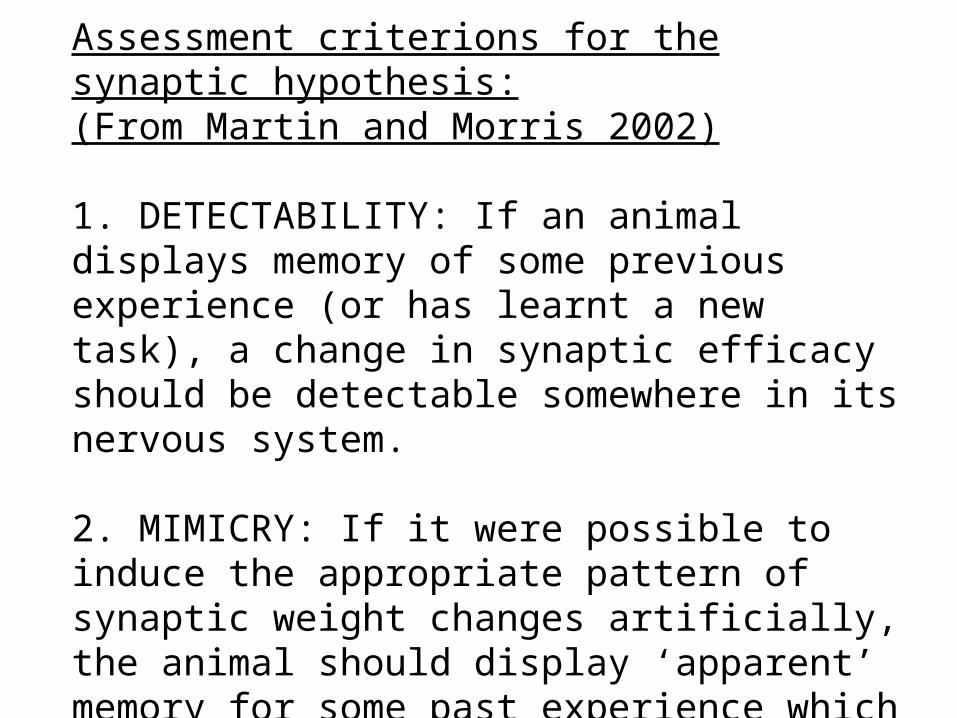
Assessment criterions for the synaptic hypothesis:(From Martin and Morris 2002)
1. DETECTABILITY: If an animal displays memory of some previous experience (or has learnt a new task), a change in synaptic efficacy should be detectable somewhere in its nervous system.
2. MIMICRY: If it were possible to induce the appropriate pattern of synaptic weight changes artificially, the animal should display ‘apparent’ memory for some past experience which did not in practice occur.Experimentally not possible.
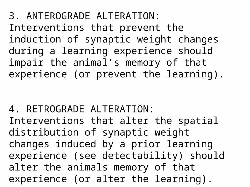
3. ANTEROGRADE ALTERATION: Interventions that prevent the induction of synaptic weight changes during a learning experience should impair the animal’s memory of that experience (or prevent the learning).
4. RETROGRADE ALTERATION: Interventions that alter the spatial distribution of synaptic weight changes induced by a prior learning experience (see detectability) should alter the animals memory of that experience (or alter the learning).
Experimentally not possible
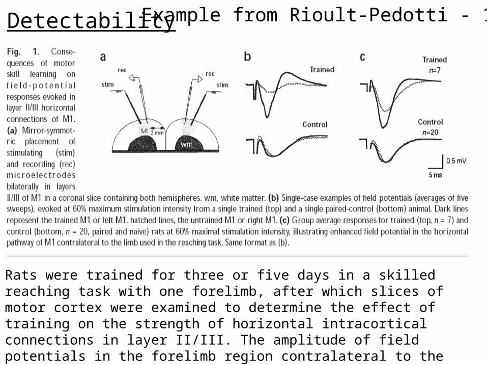
Detectability Example from Rioult-Pedotti - 1998
Rats were trained for three or five days in a skilled reaching task with one forelimb, after which slices of motor cortex were examined to determine the effect of training on the strength of horizontal intracortical connections in layer II/III. The amplitude of field potentials in the forelimb region contralateral to the trained limb was significantly increased relative to the opposite ‘untrained’ hemisphere.
ANTEROGRADE ALTERATION: Interventions that prevent the induction of synaptic weight changes during a learning experience should impair the animal’s memory of that experience (or prevent the learning).
This is the most common approach. It relies on utilizing the known properties of synaptic plasticity as induced artificially.
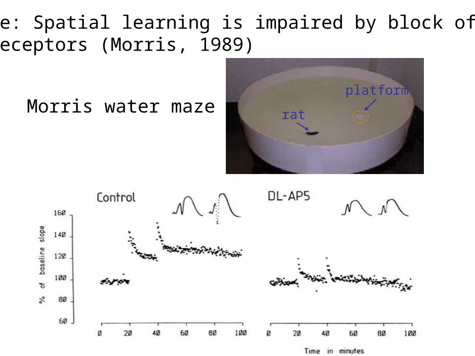
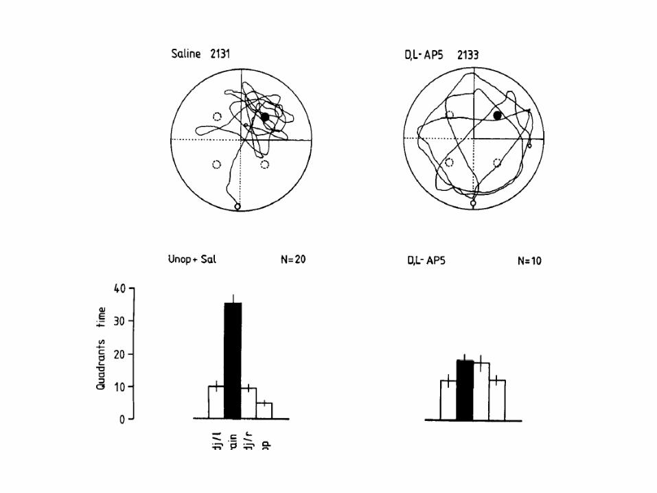
Example: Spatial learning is impaired by block of NMDA receptors (Morris, 1989)
Morris water maze rat
platform
= v u1 << 1d
dtSingle Input
= v u << 1dw
dtMany Inputs
As v is a single output, it is scalar.
Averaging Inputs= <v u> << 1
dw
dt
We can just average over all input patterns and approximate the weight change by this. Remember, this assumes that weight changes are slow.
If we replace v with w . u we can write:
= Q . w where Q = <uu> is the input correlation matrix
dw
dt
Note: Hebb yields an instable (always growing) weight vector!
Back to the Math. We had:
= (v - ) u << 1dw
dt
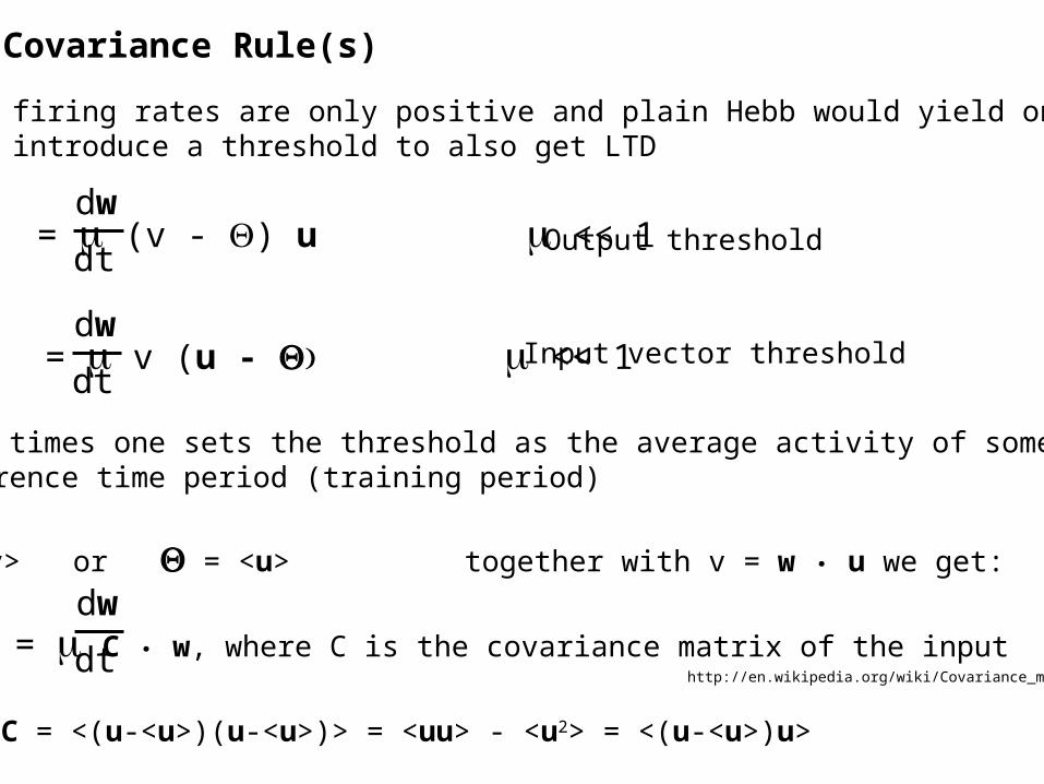
Covariance Rule(s)
Normally firing rates are only positive and plain Hebb would yield only LTP.Hence we introduce a threshold to also get LTD
Output threshold
= v (u - << 1dw
dtInput vector threshold
Many times one sets the threshold as the average activity of somereference time period (training period)
= <v> or = <u> together with v = w . u we get:
= C . w, where C is the covariance matrix of the input
dw
dthttp://en.wikipedia.org/wiki/Covariance_matrix
C = <(u-<u>)(u-<u>)> = <uu> - <u2> = <(u-<u>)u>
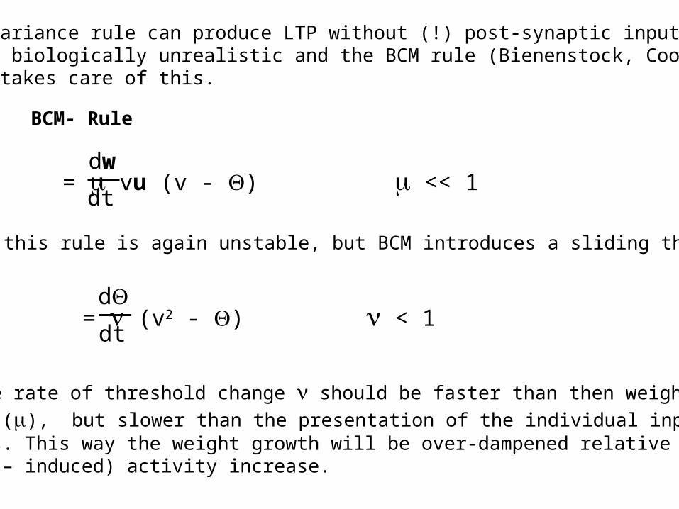
The covariance rule can produce LTP without (!) post-synaptic input.This is biologically unrealistic and the BCM rule (Bienenstock, Cooper,Munro) takes care of this.
BCM- Rule
= vu (v - ) << 1dw
dt
As such this rule is again unstable, but BCM introduces a sliding threshold
= (v2 - ) < 1d
dt
Note the rate of threshold change should be faster than then weight
changes (), but slower than the presentation of the individual inputpatterns. This way the weight growth will be over-dampened relative to the (weight – induced) activity increase.
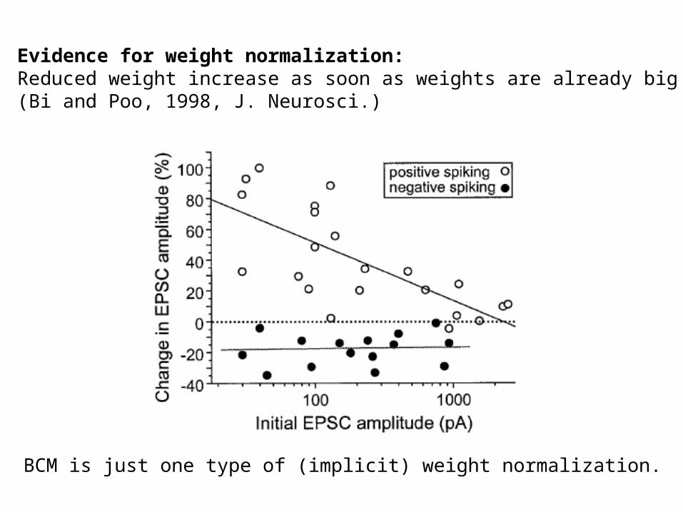
Evidence for weight normalization:Reduced weight increase as soon as weights are already big(Bi and Poo, 1998, J. Neurosci.)
BCM is just one type of (implicit) weight normalization.
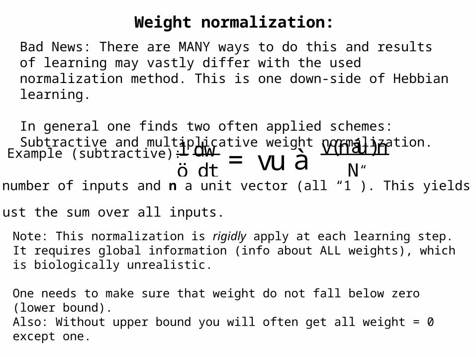
Weight normalization:
Bad News: There are MANY ways to do this and results of learning may vastly differ with the used normalization method. This is one down-side of Hebbian learning.
In general one finds two often applied schemes:Subtractive and multiplicative weight normalization.
Example (subtractive):
With N, number of inputs and n a unit vector (all “1”). This yields that
n.u is just the sum over all inputs.
Note: This normalization is rigidly apply at each learning step. It requires global information (info about ALL weights), which is biologically unrealistic.
One needs to make sure that weight do not fall below zero (lower bound).Also: Without upper bound you will often get all weight = 0 except one.
Subtractive normalization is highly competitive as the subtracted values are always the same for all weight and, hence, will affect small weight relatively more.
ö1dtdw =vu à N
v(náu)n
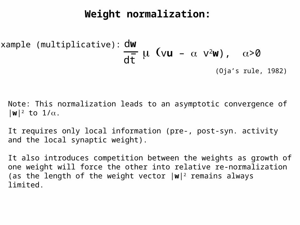
Weight normalization:
= vu – v2w), >0dw
dt
Example (multiplicative):
Note: This normalization leads to an asymptotic convergence of |w|2 to 1/.
It requires only local information (pre-, post-syn. activity and the local synaptic weight).
It also introduces competition between the weights as growth of one weight will force the other into relative re-normalization (as the length of the weight vector |w|2 remains always limited.
(Oja’s rule, 1982)
Eigen Vector Decomposition - PCA
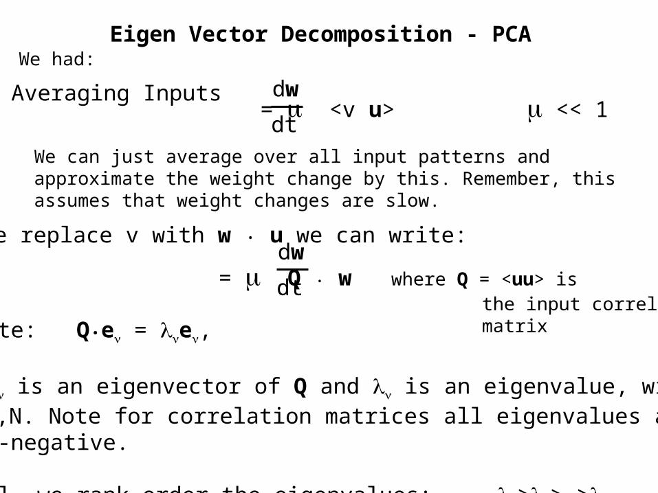
Averaging Inputs= <v u> << 1
dw
dt
We can just average over all input patterns and approximate the weight change by this. Remember, this assumes that weight changes are slow.
If we replace v with w . u we can write:
= Q . w where Q = <uu> is the input correlation matrix
dw
dt
We had:
And write: Q.e = le,
where e is an eigenvector of Q and l is an eigenvalue, with= 1,….,N. Note for correlation matrices all eigenvalues are realand non-negative.
As usual, we rank-order the eigenvalues: l1≥l2≥…≥lN
Eigen Vector Decomposition - PCA
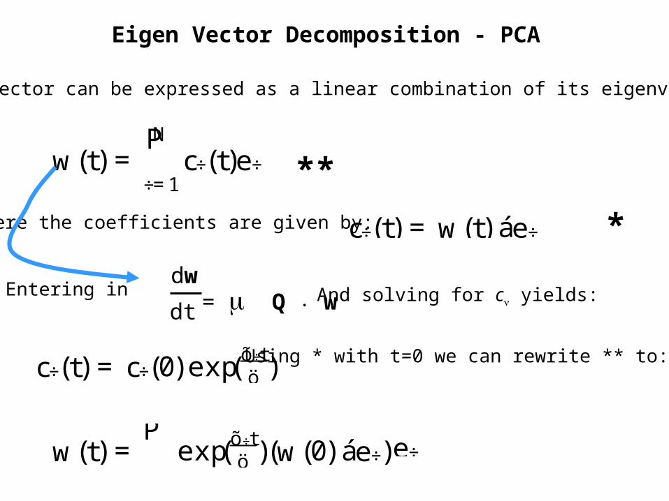
Every vector can be expressed as a linear combination of its eigenvectors:
w(t) =P
÷=1
Nc÷(t)e÷
Where the coefficients are given by: c÷(t) = w(t) áe÷ *
= Q . wdw
dtEntering in And solving for c yields:
c÷(t) = c÷(0) exp( öõ÷t) Using * with t=0 we can rewrite ** to:
**
w(t) =Pexp( ö
õ÷t)(w(0) áe÷)e÷
Eigen Vector Decomposition - PCA
w(t) =Pexp( ö
õ÷t)(w(0) áe÷)e÷
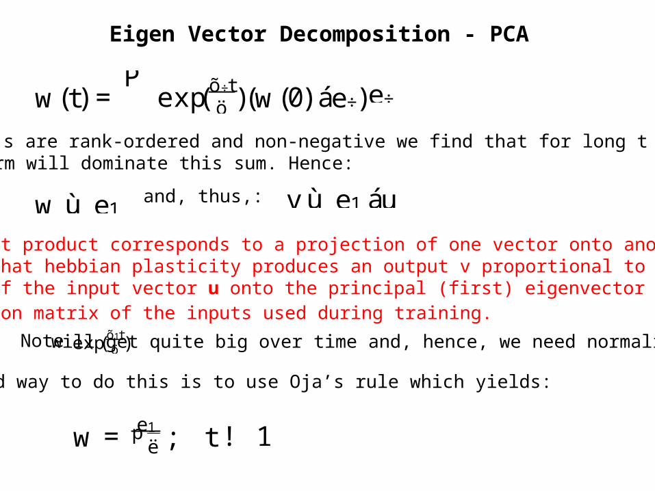
As the l’s are rank-ordered and non-negative we find that for long t only thefirst term will dominate this sum. Hence:
w ù e1 and, thus,: vù e1áu
exp( öõ1t)Note will get quite big over time and, hence, we need normalization!
As the dot product corresponds to a projection of one vector onto another,we find that hebbian plasticity produces an output v proportional to the pro-jection of the input vector u onto the principal (first) eigenvector e1 of thecorrelation matrix of the inputs used during training.
A good way to do this is to use Oja’s rule which yields:
w = ëpe1 ; t ! 1
Eigen Vector Decomposition - PCA
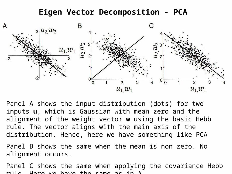
Panel A shows the input distribution (dots) for two inputs u, which is Gaussian with mean zero and the alignment of the weight vector w using the basic Hebb rule. The vector aligns with the main axis of the distribution. Hence, here we have something like PCA
Panel B shows the same when the mean is non zero. No alignment occurs.
Panel C shows the same when applying the covariance Hebb rule. Here we have the same as in A.
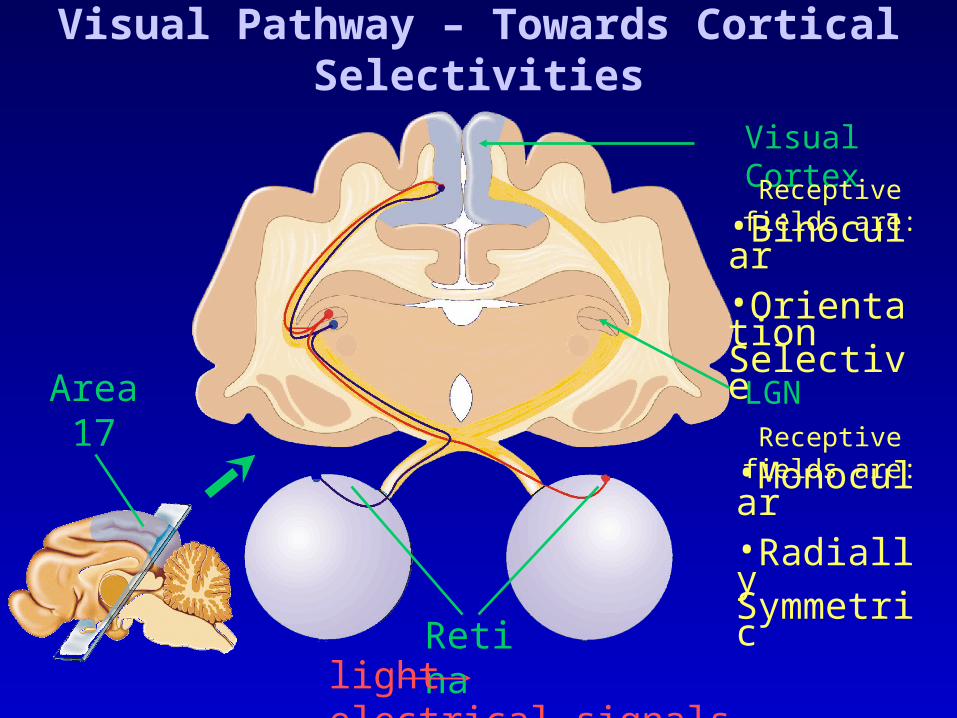
Visual Pathway – Towards Cortical Selectivities
Area17
LGN
Visual Cortex
Retinalight electrical signals
•Monocular•Radially Symmetric
•Binocular•Orientation Selective
Receptive fields are:
Receptive fields are:
Re s
pon
se (
s pik
e s/s
e c)
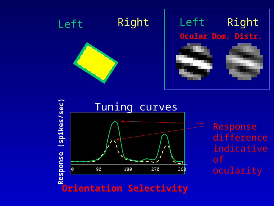
Left Right
Tuning curves
0 180 36090 270
RightLeftOcular Dom. Distr.
Orientation Selectivity
Response difference indicative of ocularity
Orientation Selectivity
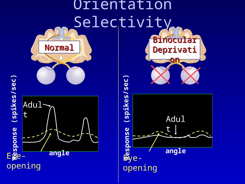
Binocular Binocular DeprivationDeprivation
NormalNormal
Adult
Eye-opening angle angle
Res
pon
se (
spik
es/s
ec)
Res
pon
se (
spik
es/s
ec)
Eye-opening
Adult
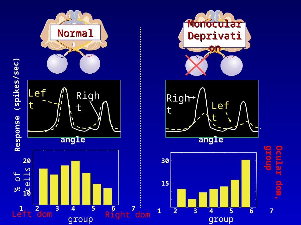
Monocular Monocular DeprivationDeprivation
NormalNormal
Left Right
% o
f ce
lls
group group
angleangleRes
pon
se (
spik
es/s
ec)
1 2 3 4 5 6 7
10
20
1 2 3 4 5 6 7
30
15
RightLeft
Oc
ular d
om
, gro
upLeft dom Right dom
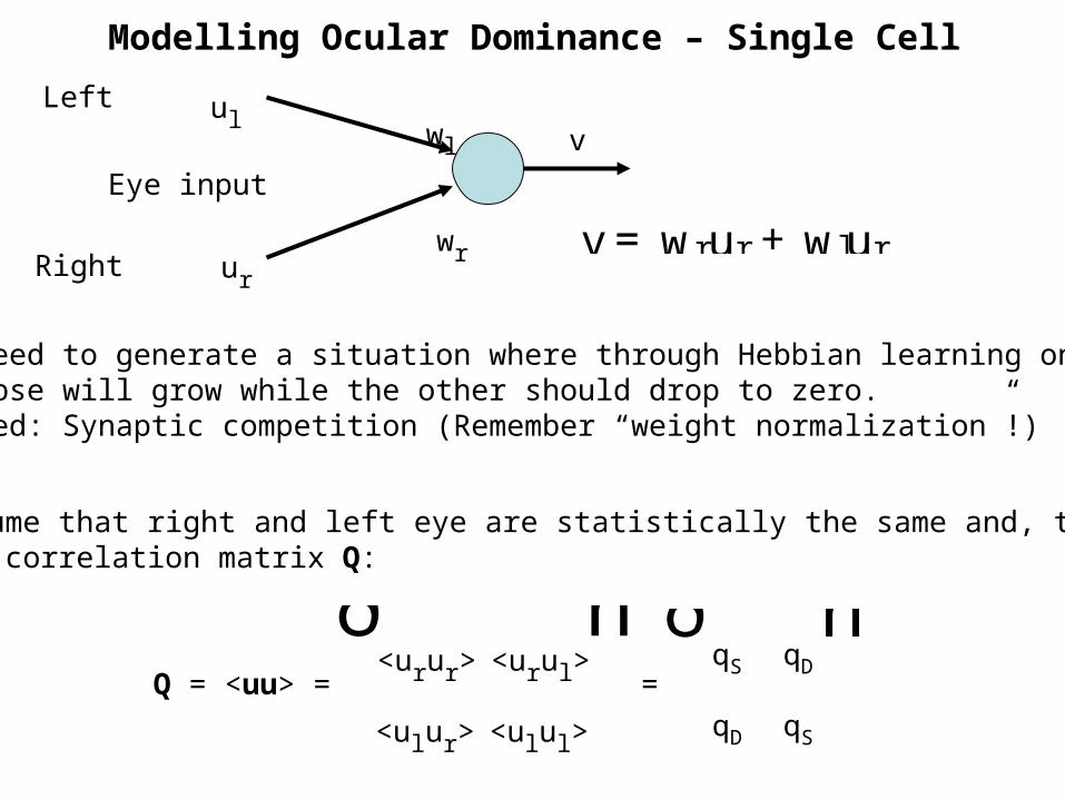
Modelling Ocular Dominance – Single Cell
Left
Right
Eye input
ul
ur
v
wr
wl
v=wrur +wlur
ð ñ<urur>
<ulur> <ulul>
<urul>Q = <uu> =
ð ñ=
qS
qD qS
qD
We need to generate a situation where through Hebbian learning onesynapse will grow while the other should drop to zero.Called: Synaptic competition (Remember “weight normalization”!)
We assume that right and left eye are statistically the same and, thus,get as correlation matrix Q:
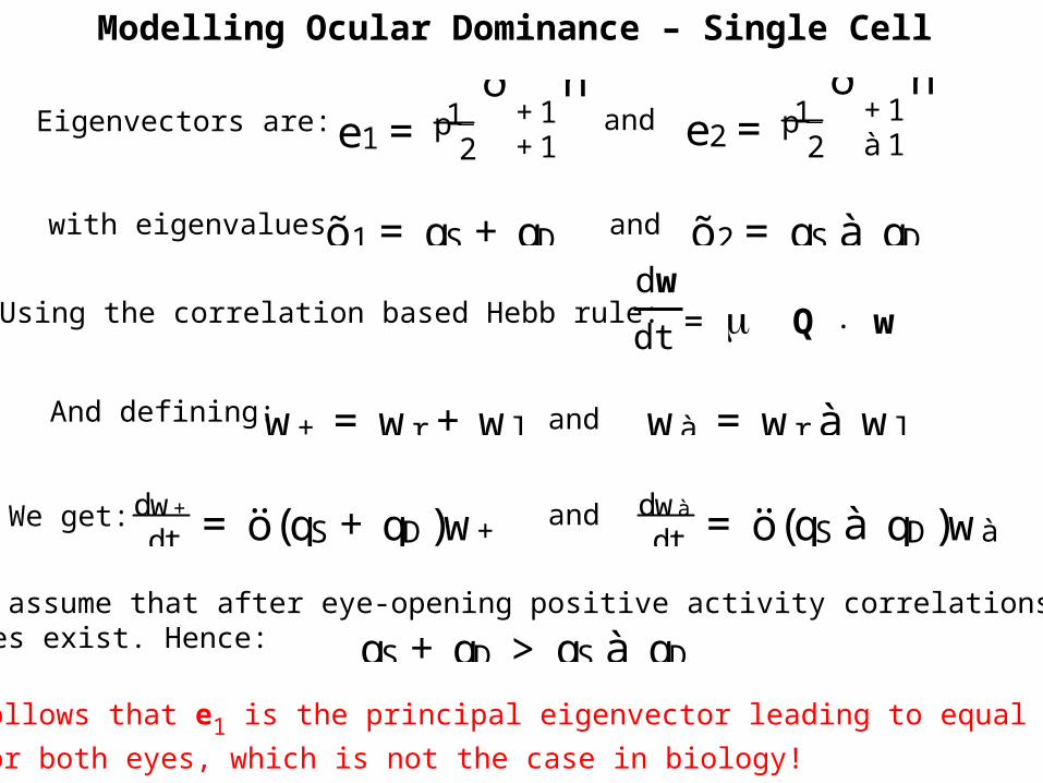
Modelling Ocular Dominance – Single Cell
Eigenvectors are: and e2= 2p1ðà1+1ñ
e1= 2p1ð+1+1ñ
õ1=qS+qD andwith eigenvalues õ2=qS à qD
Using the correlation based Hebb rule: = Q . wdw
dt
And defining: w+=wr +wl
We get:
and wà =wr à wl
dtdw+=ö(qS+qD)w+ and
dtdwà =ö(qS à qD)wà
We can assume that after eye-opening positive activity correlations betweenthe eyes exist. Hence: qS+qD >qS à qDAnd it follows that e1 is the principal eigenvector leading to equal weight
growth for both eyes, which is not the case in biology!
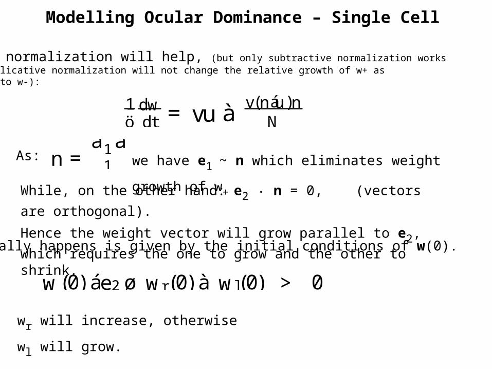
Weight normalization will help, (but only subtractive normalization worksas multiplicative normalization will not change the relative growth of w+ ascompared to w-):
ö1dtdw =vu à N
v(náu)n
Modelling Ocular Dominance – Single Cell
As: n =à11á
we have e1 ~ n which eliminates weight growth of w+
While, on the other hand: e2 . n = 0, (vectors are orthogonal).
Hence the weight vector will grow parallel to e2, which requires the
one to grow and the other to shrink.What really happens is given by the initial conditions of w(0).
If: w(0) áe2ø wr(0) à wl(0) > 0
wr will increase, otherwise wl will grow.
Modelling Ocular Dominance – Networks
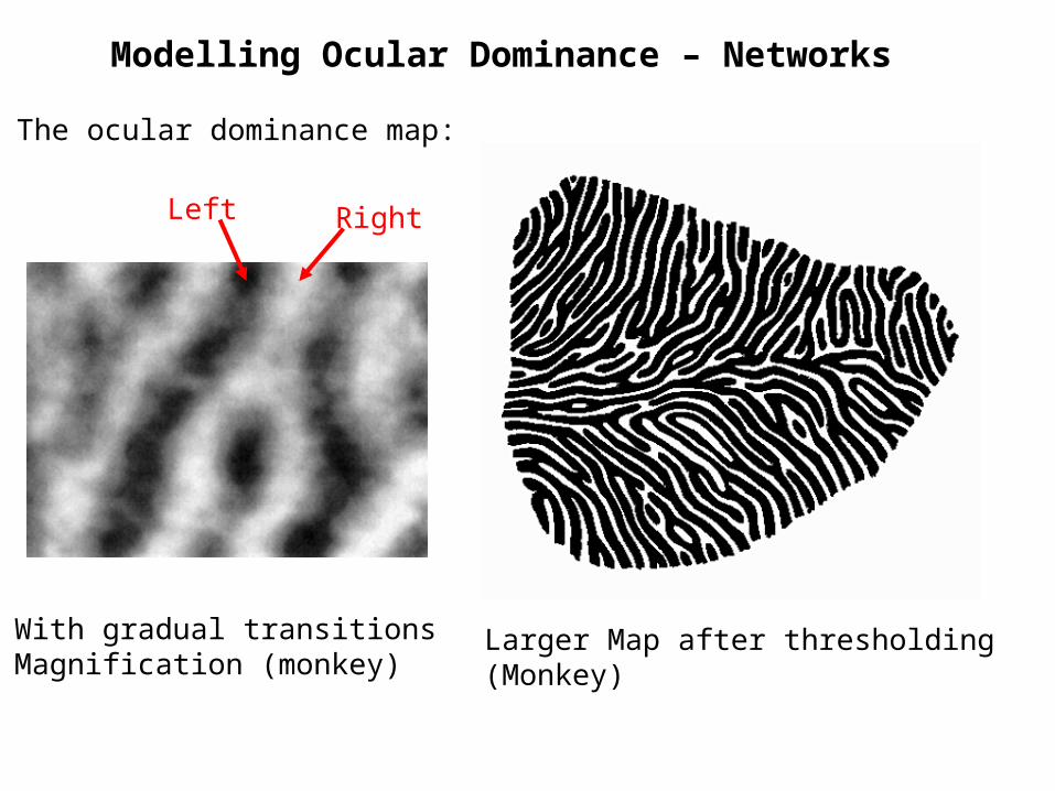
The ocular dominance map:
With gradual transitionsMagnification (monkey)
Larger Map after thresholding(Monkey)
Left Right
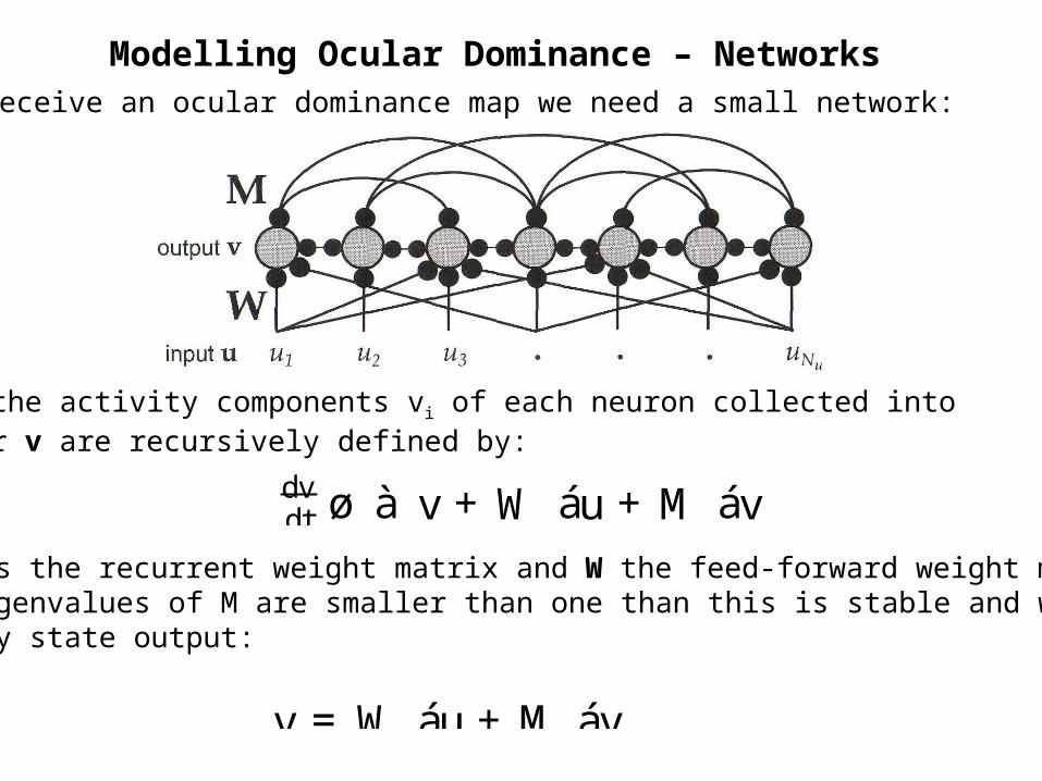
Modelling Ocular Dominance – NetworksTo receive an ocular dominance map we need a small network:
dtdv ø à v +W áu+M áv
Here the activity components vi of each neuron collected into vector v are recursively defined by:
Where M is the recurrent weight matrix and W the feed-forward weight matrix.If the eigenvalues of M are smaller than one than this is stable and we get asthe steady state output:
v =W áu+M áv
Modelling Ocular Dominance – Networks
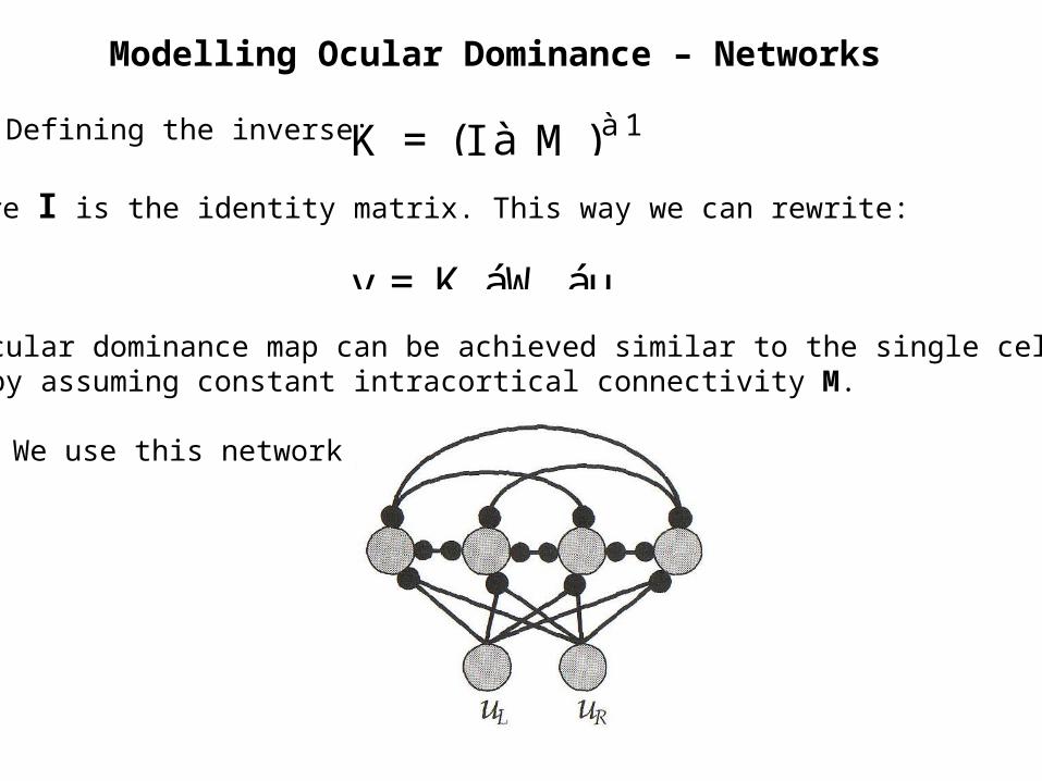
Defining the inverse: K = (I à M )à1
Where I is the identity matrix. This way we can rewrite:
v = K áW áu
An ocular dominance map can be achieved similar to the single cell modelbut by assuming constant intracortical connectivity M.
We use this network:
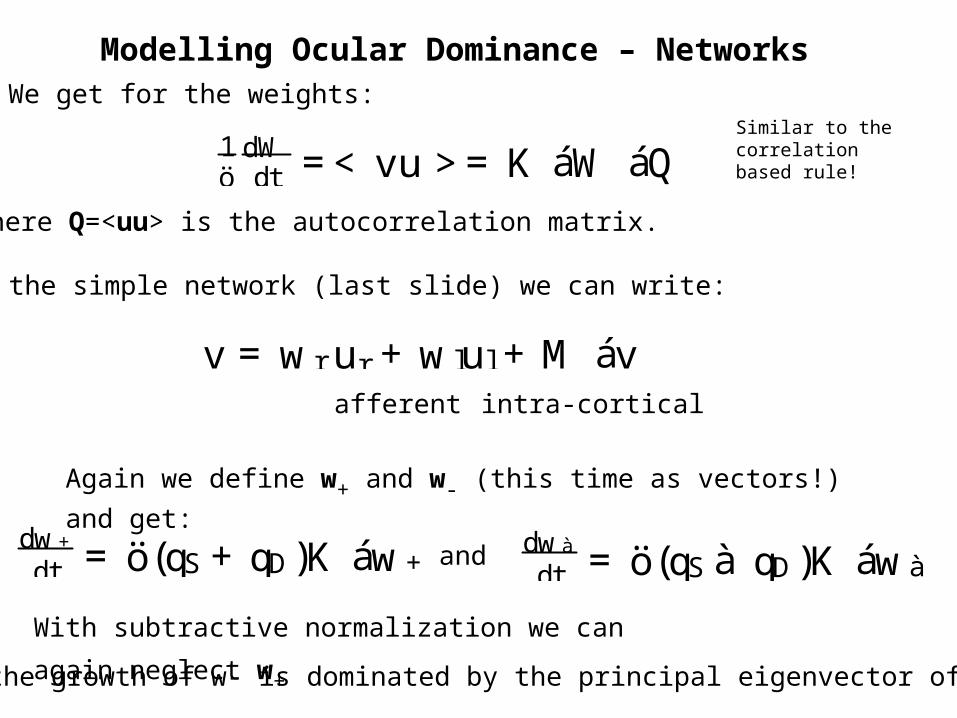
Modelling Ocular Dominance – NetworksWe get for the weights:
ö1dtdW =<vu >=K áW áQ
where Q=<uu> is the autocorrelation matrix.
Similar to the correlation based rule!
For the simple network (last slide) we can write:
v =wr ur +wlul+M ávafferent intra-cortical
Again we define w+ and w- (this time as vectors!) and get:
dtdw+=ö(qS+qD)K áw+ and
dtdwà =ö(qS à qD)K áwà
With subtractive normalization we can again neglect w+Hence the growth of w- is dominated by the principal eigenvector of K
Modelling Ocular Dominance – Networks
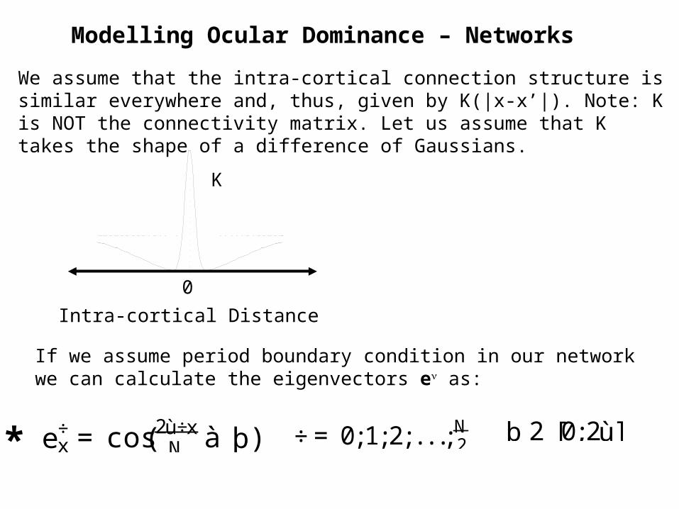
We assume that the intra-cortical connection structure is similar everywhere and, thus, given by K(|x-x’|). Note: K is NOT the connectivity matrix. Let us assume that K takes the shape of a difference of Gaussians.
K
Intra-cortical Distance
0
If we assume period boundary condition in our network we can calculate the eigenvectors e as:
þ 2 [0;2ù]e÷x = cos( N2ù÷x à þ) ÷=0;1;2; . . .; 2
N*
Modelling Ocular Dominance – Networks
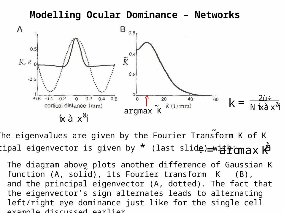
The eigenvalues are given by the Fourier Transform K of K~
The principal eigenvector is given by * (last slide) with: ÷=argmaxKà
The diagram above plots another difference of Gaussian K function (A, solid), its Fourier transform K (B), and the principal eigenvector (A, dotted). The fact that the eigenvector’s sign alternates leads to alternating left/right eye dominance just like for the single cell example discussed earlier.
~
k = Njxàx0j2ù÷
jx à x0jargmax K
~