Overview of Unstructured Mesh Generation Methods

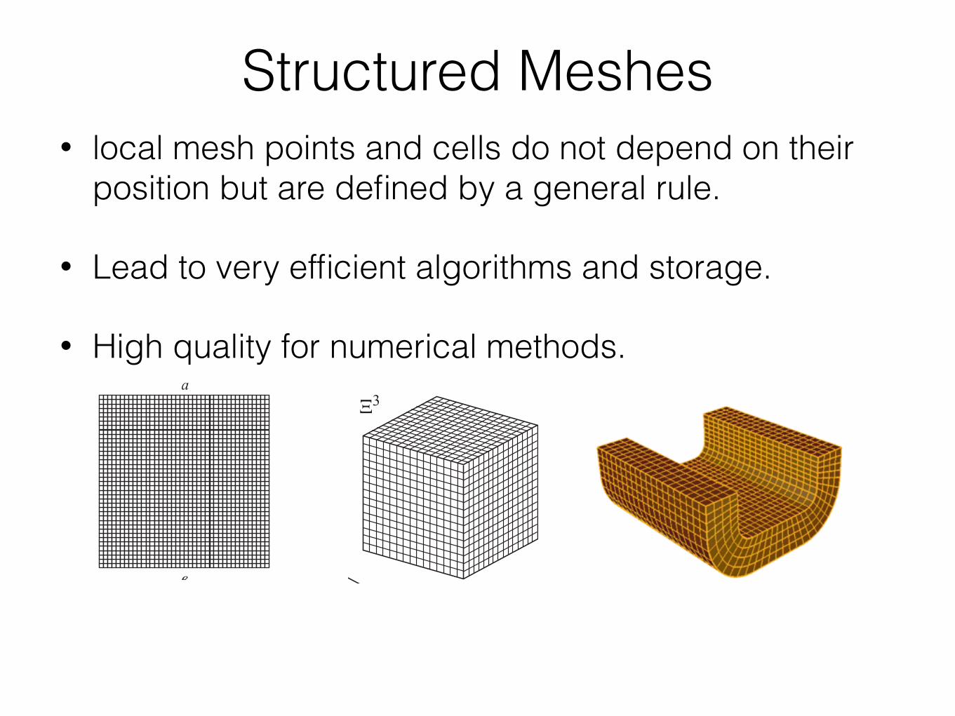
Structured Meshes• local mesh points and cells do not depend on their

position but are defined by a general rule.

• Lead to very efficient algorithms and storage.

• High quality for numerical methods.

186 gLAWA 8. ~ISLENNOE RE[ENIE SINGULQRNO WOZMU]ENNYH ZADA^

rIS. 8.11. dWUMERNAQ SETKA I RE[ENIE ZADA^I (8.39), POSTROENNOENA NEJ DLQ " = 0,0005:

A — RAWNOMERNAQ SETKA; B — ADAPTIWNAQ SETKA

rIS. 8.12. pOKAZATELX SHODIMOSTI ↵N

RE[ENIQ ZADA^I (8.39) NAADAPTIWNOJ SETKE

4.1. bAZISNYE FUNKCIONALY I URAWNENIQ 77

rIS. 4.1. sHEMA POSTROENIQ GEKSA\DRALXNYH SETOK

ORDINATAH v1, . . . , vn, KAK gxv

ij

(gij

vx

), TAKIM OBRAZOM W SETO^NYH KOORDINATAH

⇠1, . . . , ⇠n

gx⇠

ij

= x⇠

i

· x⇠

j

=@xk

@⇠i

@xk

@⇠j

, gij

⇠x

=@⇠i

@xk

@⇠j

@xk

, i, j, k = 1, . . . , n. (4.2)

nAPOMNIM, ^TO, SOGLASNO PRINQTOMU RANEE PRAWILU, W (4.2) I DALEE W MATEMA-TI^ESKIH WYRAVENIQH, IME@]IH ODINAKOWYE INDEKSY I NE WKL@^A@]IH ZNAKI

+, � ILI =, S^ITAETSQ, ^TO PO \TIM INDEKSAM PROWEDENO SUMMIROWANIE, ESLI NEGOWORITSQ OBRATNOE.

4.1.2. uPRAWLQ@]AQ METRIKAw RASSMATRIWAEMOJ ZDESX WERSII METODA OTOBRAVENIJ DLQ \FFEKTIWNOGO KON-

TROLIROWANIQ SWOJSTW SETOK W OBLASTI Xn WWODITSQ PONQTIE MONITORNOGO MNOGO-OBRAZIQ NAD Xn. tO^KAMI MNOGOOBRAZIQ QWLQ@TSQ TO^KI Xn, TOGDA KAK METRIKA\TOGO MNOGOOBRAZIQ MOVET OTLI^ATXSQ OT METRIKI OBLASTI Xn. mY BUDEM SSY-LATXSQ NA \TU BOLEE OB]U@ METRIKU KAK NA UPRAWLQ@]U@ METRIKU. oBOZNA^IMKOWARIANTNYE (KONTRAWARIANTNYE) \LEMENTY UPRAWLQ@]EJ METRIKI W KOORDINA-TAH v1, . . . , vn KAK gv

ij

(gij

v

).

oTMETIM, ^TO MATRICY {gv

ij

} I {gij

v

}, NAZYWAEMYE SOOTWETSTWENNO KOWARI-ANTNYM I KONTRAWARIANTNYM METRI^ESKIMI TENZORAMI W KOORDINATAH v1, . . . , vn,DOLVNY UDOWLETWORQTX OPREDELENIQM METRI^ESKIH TENZOROW, A IMENNO BYTX NEWY-ROVDENNYMI, SIMMETRI^NYMI I WZAIMNO-OBRATNYMI, T. E.

gv

ij

gjk

v

= �i

k

, i, j, k = 1, . . . , n, (4.3)

GDE �i

k

— SIMWOL kRONEKERA, T. E. �i

k

= 1 PRI i = k I �i

k

= 0 PRI i 6= k. i KROMETOGO, PRI PEREHODE OT SISTEMY KOORDINAT v1, . . . , vn K NOWOJ SISTEME w1, . . . , wn

\LEMENTY KOWARIANTNYH METRI^ESKIH TENZOROW W STARYH I NOWYH KOORDINATAH

DOLVNY BYTX SWQZANY SOOTNO[ENIQMI, KOTORYE WERNY DLQ KOWARIANTNYH TENZO-ROW WTOROGO RANGA:

gv

ij

= gw

kp

@wk

@vi

@wp

@vj

, i, j, k, p = 1, . . . , n. (4.4)

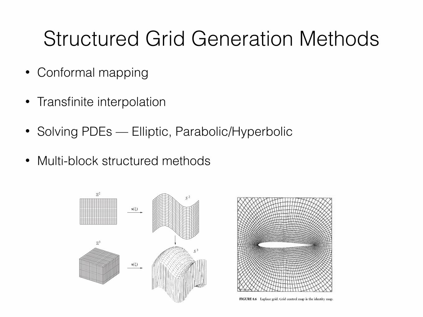
Structured Grid Generation Methods• Conformal mapping

• Transfinite interpolation

• Solving PDEs — Elliptic, Parabolic/Hyperbolic

• Multi-block structured methods5.3. wY^ISLITELXNYE ALGORITMY 133

rIS. 5.10. pOSLEDOWATELXNYJ PROCESS POSTROENIQ GEKSA\DRALXNYHSETOK

tAK VE KAK I DLQ POSTROENIQ SETOK W OBLASTQH, RE[ENIQ PREOBRAZOWANNYHNELINEJNYH KRAEWYH ZADA^ (5.67) I (5.69) MOGUT BYTX NAJDENY SLEDU@]IM OBRA-ZOM.oNI ZAMENQ@TSQ NA NESTACIONARNYE KRAEWYE ZADA^I OTNOSITELXNO KOMPONENTsi(⇠, t), i = 1, . . . , n, WEKTORNOJ FUNKCII s(⇠, t) : ⌅n ⇥ [0, T ]! Sn:

@si

@t= (J)p

n

B⇠n

[si]�Ri[s]o

, i, j,m = 1, . . . , n,

si(⇠, t) = i(⇠), ⇠ 2 @⌅n, t � 0, si(⇠, 0) = si

0

(⇠) , ⇠ 2 ⌅n,

(5.72)

GDE DLQ (5.67)

Ri[s] = (J)2p

gs

@

@⇠j(p

gsgim

s

)@⇠j

@sm

, i, j,m = 1, . . . , n, (5.73)

A DLQ (5.69)

Ri[s] =gs(J)2

w1

(s)@

@⇠k(w

1

(s)gij

s

)@⇠k

@sj

, i, j, k = 1, . . . , n,

• Only suitable for domain with regular shapes.

• The block-structured (or hybrid) mesh is formed by a number of structured meshes combined in an unstructured pattern.

• Mesh adaptation is difficult.

Limitations of Structured Meshes

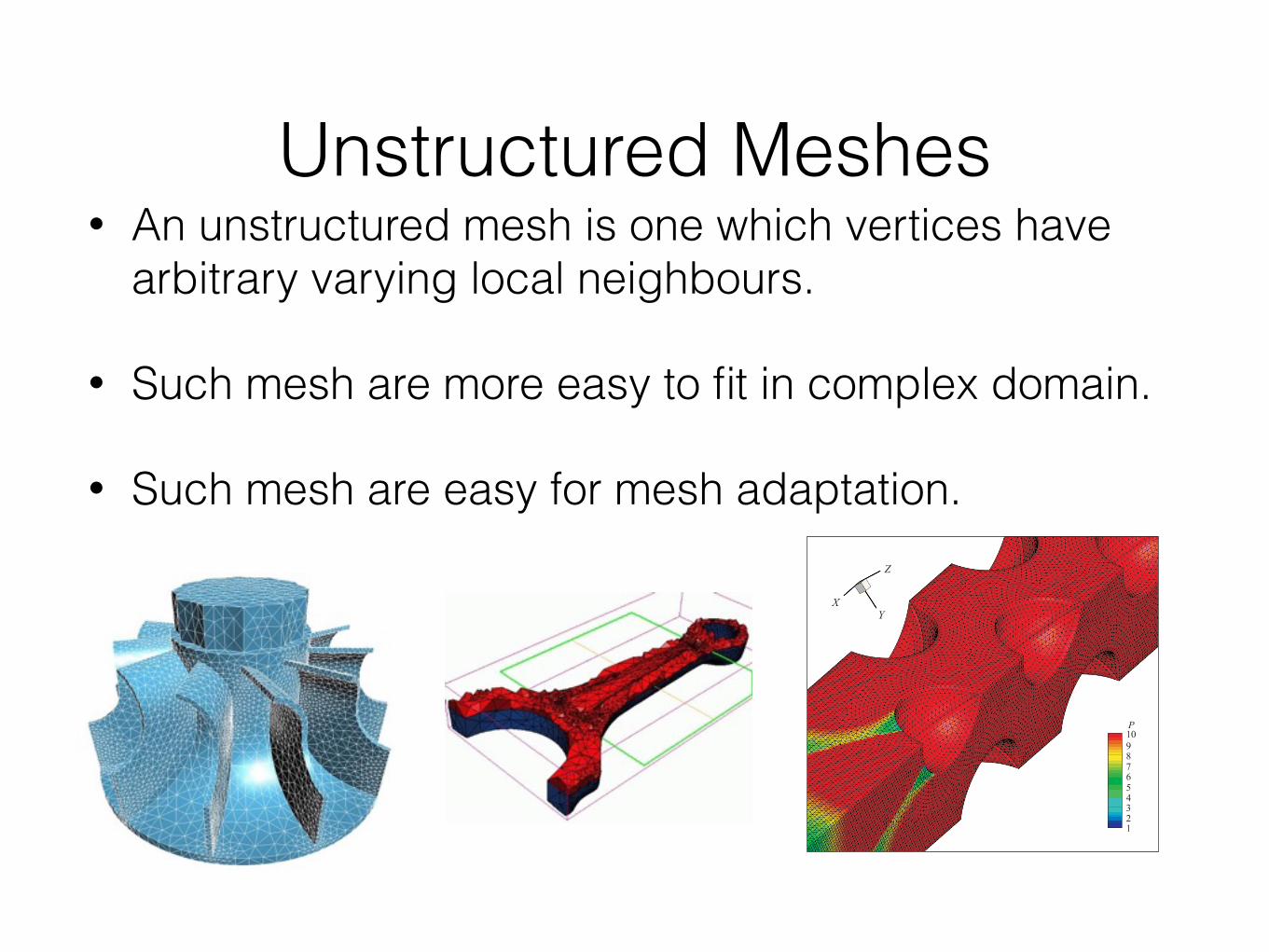
Unstructured Meshes• An unstructured mesh is one which vertices have

arbitrary varying local neighbours.

• Such mesh are more easy to fit in complex domain.

• Such mesh are easy for mesh adaptation.9.4. ~ISLENNOE MODELIROWANIE NAKATA WOLNY CUNAMI 199

rIS. 9.7. fRAGMENT POSTROENNOJ TREHMERNOJ SETKI

9.4. ~ISLENNOE MODELIROWANIE NAKATAWOLNY CUNAMI

qPONSKIJ TERMIN «CUNAMI» OZNA^AET NABEGA@]U@ NA POBEREVXE BOLX[U@

WOLNU, WYZWANNU@ PODWODNYM ZEMLETRQSENIEM, IZWERVENIEM PODWODNOGO WULKANAILI PODWODNYM OPOLZNEM. |TO OPASNOE PO SWOIM POSLEDSTWIQM PRIRODNOE QWLENIE^ASTO PRIWODIT K GIGANTSKIM PO SWOIM MAS[TABAM RAZRU[ENIQM I GIBELI BOLX-[OGO ^ISLA L@DEJ. pRI RAZRABOTKE SREDSTW PROGNOZIROWANIQ POSLEDSTWIJ TAKOGOQWLENIQ KL@^EWU@ ROLX IGRAET ^ISLENNOE MODELIROWANIE PROCESSOW WOZNIKNOWE-NIQ I RASPROSTRANENIQ WOLN CUNAMI, A TAKVE IH NAKATA NA POBEREVXE. oSNOWNOJCELX@ MODELIROWANIQ QWLQETSQ OPERATIWNAQ (W TE^ENIE NESKOLXKIH MINUT) OCEN-KA S POMO]X@ KOMPX@TERNYH RAS^ETOW ZON ZATOPLENIQ I MAKSIMALXNYH WYSOT

ZAPLESKA WODY NA SU[E. zADA^I TAKOGO KLASSA ISSLEDU@TSQ METODAMI WOLNOWOJGIDRODINAMIKI SO SWOBODNOJ POWERHNOSTX@, I DLQ IH RE[ENIQ RAZRABOTANO DO-STATO^NO MNOGO ^ISLENNYH METODOW. oDNIM IZ POPULQRNYH W POSLEDNIE GODY STALBESSETO^NYJ METOD SPH (Smoothed Particle Hydrodynamics), QWLQ@]IJSQ DALX-NEJ[IM RAZWITIEM METODA ^ASTIC W Q^EJKAH (PIC). w OTLI^IE OT METODA PIC W

SPH OTSUTSTWUET \JLEROW \TAP. |TO POZWOLILO, S ODNOJ STORONY, SDELATX METODBOLEE \FFEKTIWNYM, NADEVNYM I PRIMENIMYM DLQ RAS^ETA TE^ENIJ W SLOVNYHOBLASTQH, NO, S DRUGOJ STORONY, TREBU@]IM RAZRABOTKI RQDA SLOVNYH PROCEDURSGLAVIWANIQ DLQ OPISANIQ WZAIMODEJSTWIQ MEVDU ^ASTICAMI, ^TO NE OBESPE^IWA-ET POLNU@ KONSERWATIWNOSTX METODA. w METODE KRUPNYH ^ASTIC (k~), PRIMENQE-

• Quadtree-Octree based methods

• Advancing-front methods

• Delaunay-based methods

Quadtree-Octree based Methods

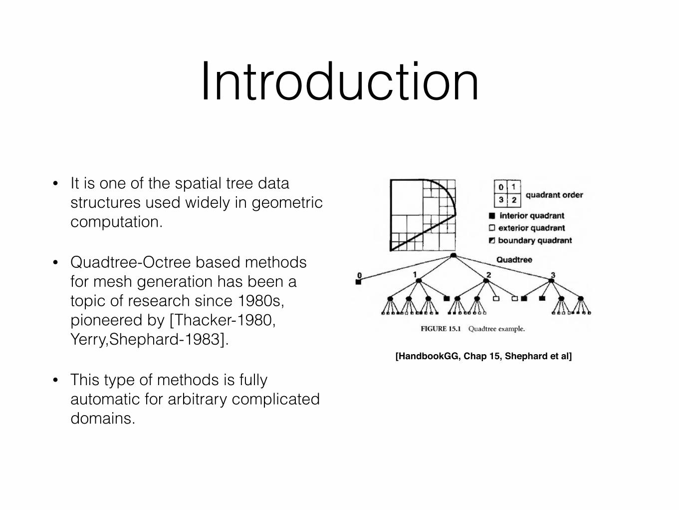
Introduction• It is one of the spatial tree data

structures used widely in geometric computation.

• Quadtree-Octree based methods for mesh generation has been a topic of research since 1980s, pioneered by [Thacker-1980, Yerry,Shephard-1983].

• This type of methods is fully automatic for arbitrary complicated domains.

[HandbookGG, Chap 15, Shephard et al]

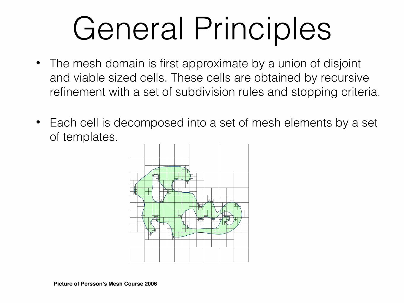
General Principles• The mesh domain is first approximate by a union of disjoint

and viable sized cells. These cells are obtained by recursive refinement with a set of subdivision rules and stopping criteria.

• Each cell is decomposed into a set of mesh elements by a set of templates.

Mesh Size Functions

• Function h(x) specifying desired mesh element size

• Many mesh generators need a priori mesh size functions

– Physically-based methods such as DistMesh

– Advancing front and Paving methods

• Discretize mesh size function h(x) on a coarse background grid

12Picture of Persson’s Mesh Course 2006

10

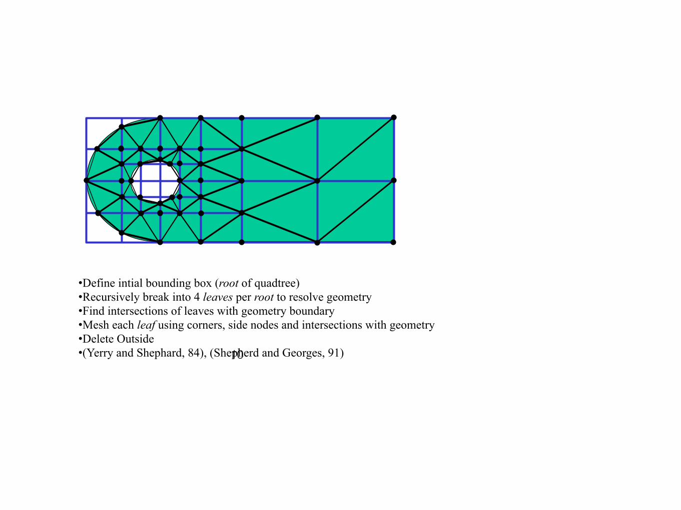
•Define intial bounding box (root of quadtree) •Recursively break into 4 leaves per root to resolve geometry •Find intersections of leaves with geometry boundary •Mesh each leaf using corners, side nodes and intersections with geometry •Delete Outside •(Yerry and Shephard, 84), (Shepherd and Georges, 91)

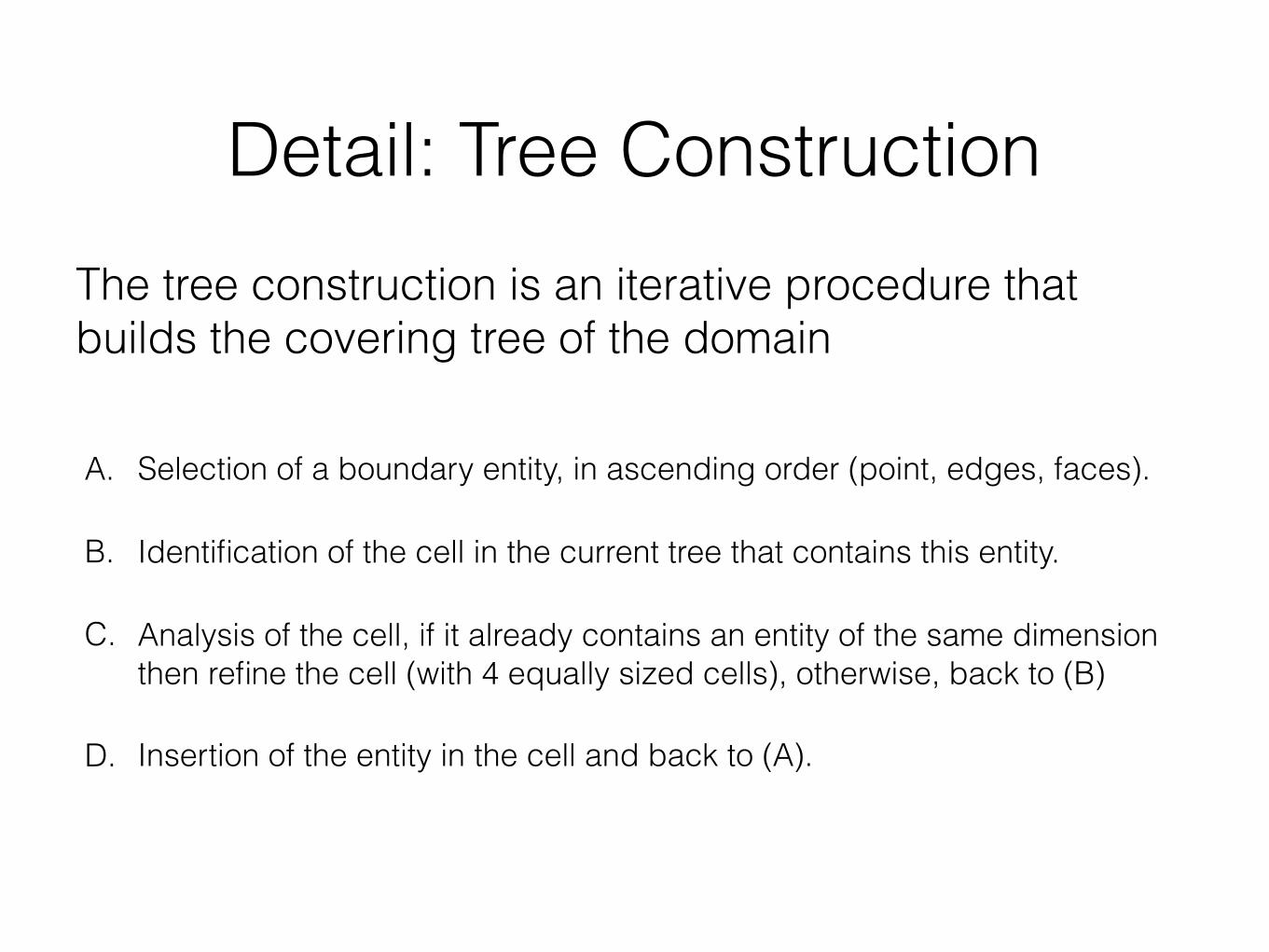
Detail: Tree Construction

A. Selection of a boundary entity, in ascending order (point, edges, faces).

B. Identification of the cell in the current tree that contains this entity.

C. Analysis of the cell, if it already contains an entity of the same dimension then refine the cell (with 4 equally sized cells), otherwise, back to (B)

D. Insertion of the entity in the cell and back to (A).

The tree construction is an iterative procedure that builds the covering tree of the domain

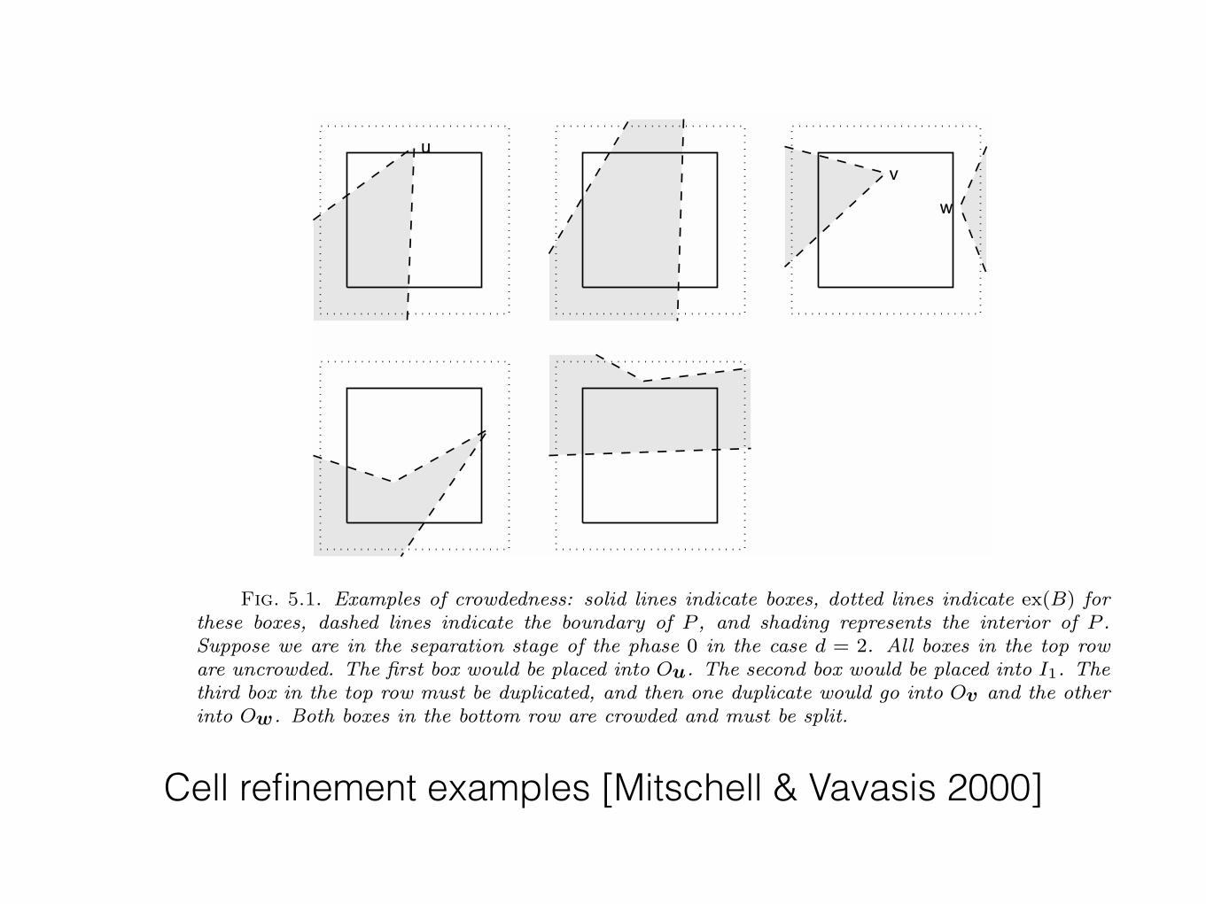
Cell refinement examples [Mitschell & Vavasis 2000]

1340 SCOTT A. MITCHELL AND STEPHEN A. VAVASIS

uv

w

Fig. 5.1. Examples of crowdedness: solid lines indicate boxes, dotted lines indicate ex(B) forthese boxes, dashed lines indicate the boundary of P , and shading represents the interior of P .Suppose we are in the separation stage of the phase 0 in the case d = 2. All boxes in the top roware uncrowded. The first box would be placed into O

u

. The second box would be placed into I1

. Thethird box in the top row must be duplicated, and then one duplicate would go into O

v

and the otherinto O

w

. Both boxes in the bottom row are crowded and must be split.

boundary faces), but in practice the running time will usually be closer to O(n).In the case d = 2, it is possible to find connected components of co(B) via a plane

sweep in O(n logn) operations. In the case d = 3, an O(n logn) plane sweep can alsobe used provided that P is preprocessed with O(N2) preprocessing steps, where N isthe combinatorial complexity of the input polyhedron P . This e�cient algorithm ford = 3 is described in our earlier paper [13]. We have not implemented a plane-sweepprocedure for either d = 2 or d = 3.

6. Alignment. In this section we describe the alignment stage. Recall that thealignment stage processes each orbit independently. For this section, assume we arein phase k and are processing orbit OF of P -face F whose dimension is k.

First, a sequence of parameters

0 = ✏d,F = ✏d�1,F = · · · = ✏d�k,F < ✏d�k�1,F < ✏d�k�2,F < · · · < ✏0,F < 0.5

is chosen for F . The method for choosing positive scalars ✏d�k�1,F , ✏d�k�2,F , . . . , ✏0,Fis described in [12], which must be slightly modified to take into account the contain-ment relationship between P -faces of di↵erent dimensions. These parameters havepositive upper and lower bounds depending only on d and k.

We now process boxes in OF in the order described below. Let B be the high-precedence box in the orbit. Let B0 be any subface of B. We construct the 1-norm neighborhood of radius ✏r,F around B0, denoted N(B0), where r stands for thedimension of B0. Thus, this neighborhood is an axis-parallel parallelepiped (whichcould be degenerate if ✏r,F = 0). If F meets N(B0), then F is said to be close to B0.The close subface of B is the box subface of lowest dimension that is close to F . Ifthere is a tie (i.e., there are several faces of the same lowest dimension all close to F ),then we break the tie with a priority rule, which is described below. A box with noclose subface is transferred to Ik+1.

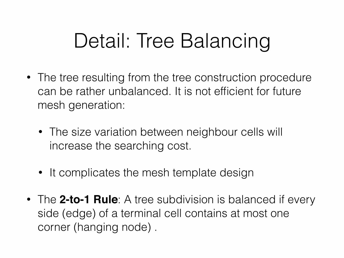
Detail: Tree Balancing• The tree resulting from the tree construction procedure

can be rather unbalanced. It is not efficient for future mesh generation:

• The size variation between neighbour cells will increase the searching cost.

• It complicates the mesh template design

• The 2-to-1 Rule: A tree subdivision is balanced if every side (edge) of a terminal cell contains at most one corner (hanging node) .

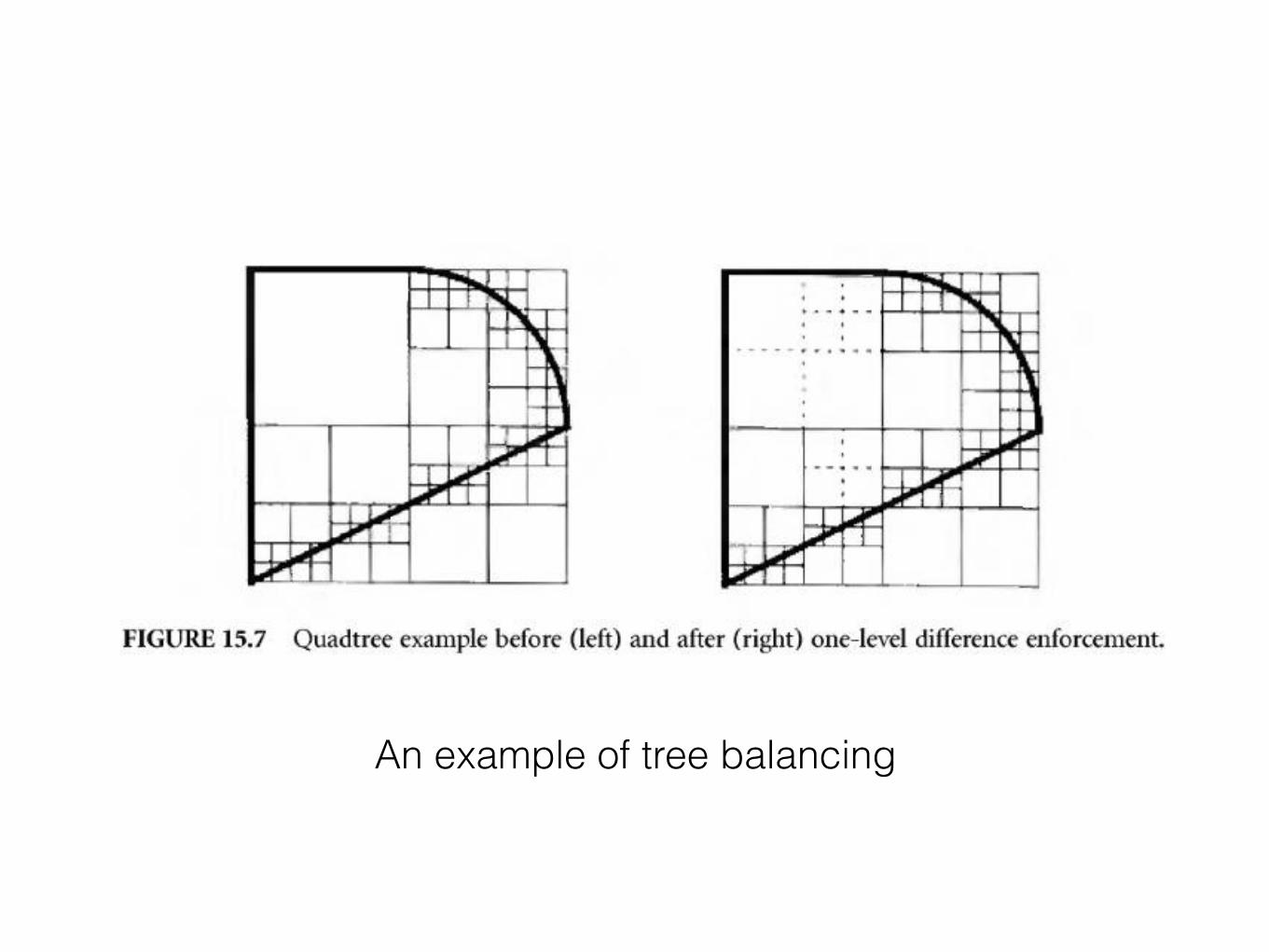
An example of tree balancing

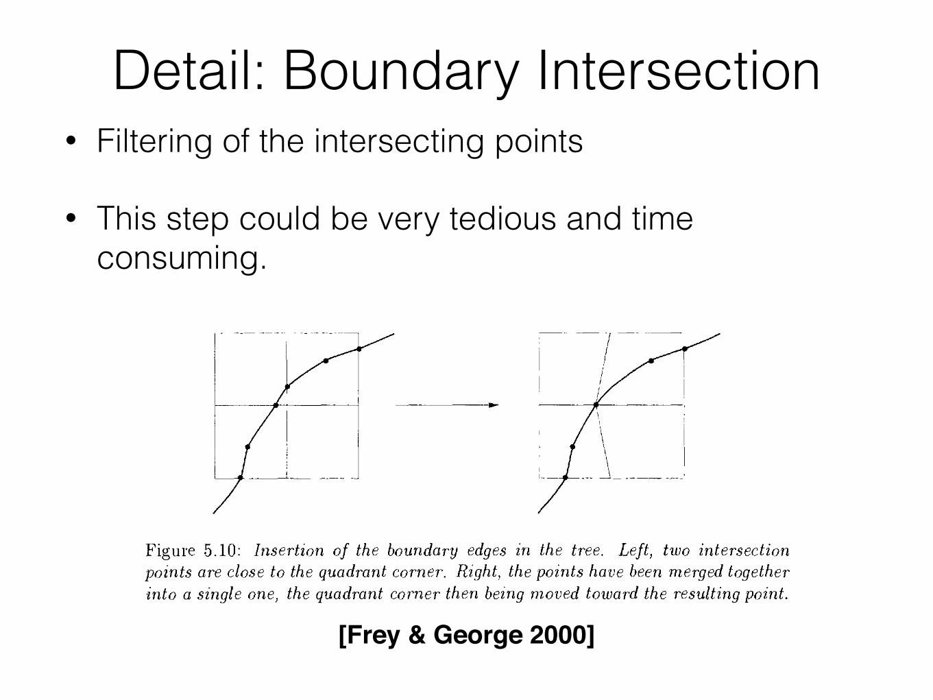
Detail: Boundary Intersection• Filtering of the intersecting points

• This step could be very tedious and time consuming.

[Frey & George 2000]

[Mitschell & Vavasis 2000]

1342 SCOTT A. MITCHELL AND STEPHEN A. VAVASIS

E

a

b

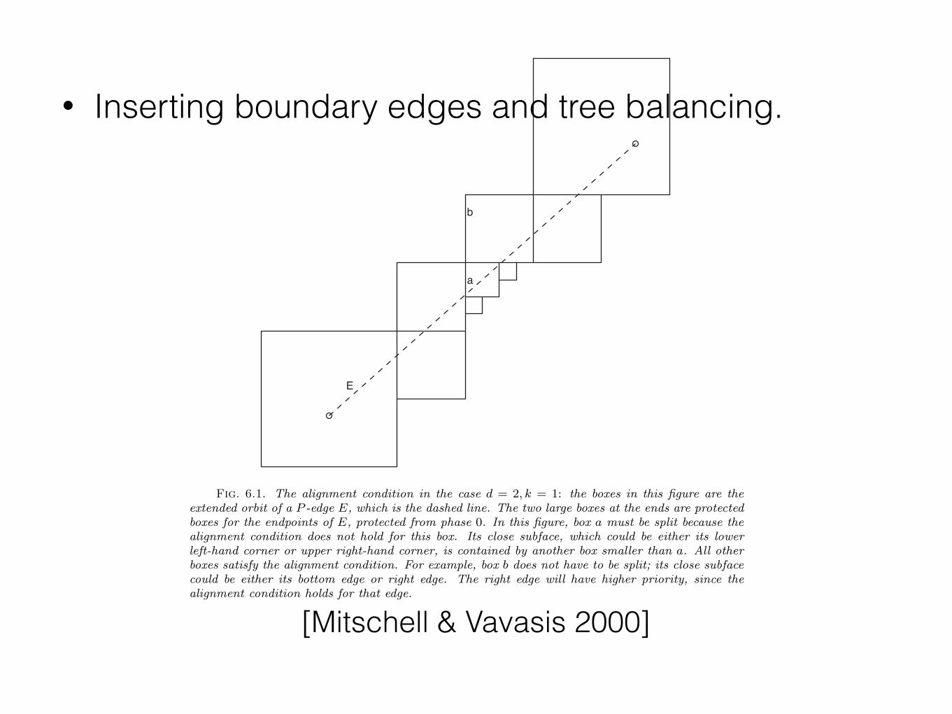
Fig. 6.1. The alignment condition in the case d = 2, k = 1: the boxes in this figure are theextended orbit of a P -edge E, which is the dashed line. The two large boxes at the ends are protectedboxes for the endpoints of E, protected from phase 0. In this figure, box a must be split because thealignment condition does not hold for this box. Its close subface, which could be either its lowerleft-hand corner or upper right-hand corner, is contained by another box smaller than a. All otherboxes satisfy the alignment condition. For example, box b does not have to be split; its close subfacecould be either its bottom edge or right edge. The right edge will have higher priority, since thealignment condition holds for that edge.

could not end up in OF (i.e., if they were still active in phase dim(F ), they would becrowded).

As mentioned earlier, a box is protected if the alignment condition holds for itsclose subface. We make the following claim: if the alignment condition holds for B atthe time it is protected, then the condition continues to hold for the remainder of thealgorithm. In other words, the following situation cannot occur: a box B with closesubface B0 is deemed to satisfy the alignment condition and becomes protected. Latera neighboring box B̄ also containing B0 as a subface gets split because the alignmentcondition does not hold for B̄, thus causing the alignment condition to be violatedfor B.

To prove the claim in the last paragraph, we must describe the order in whichQMG processes the boxes in an orbit OF . “Process” means that QMG determineswhether the box satisfies the alignment condition; if so, then protect it, and if not,then split it. The correct order is to start with the largest boxes in the orbit, workingdown to the smallest. Within the set of boxes of the same size, we process those withthe lowest-dimensional close subfaces first, working toward highest-dimensional closesubfaces.

• Inserting boundary edges and tree balancing.

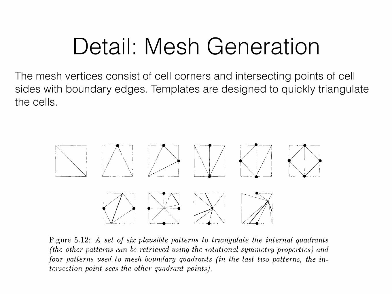
Detail: Mesh GenerationThe mesh vertices consist of cell corners and intersecting points of cell sides with boundary edges. Templates are designed to quickly triangulate the cells.

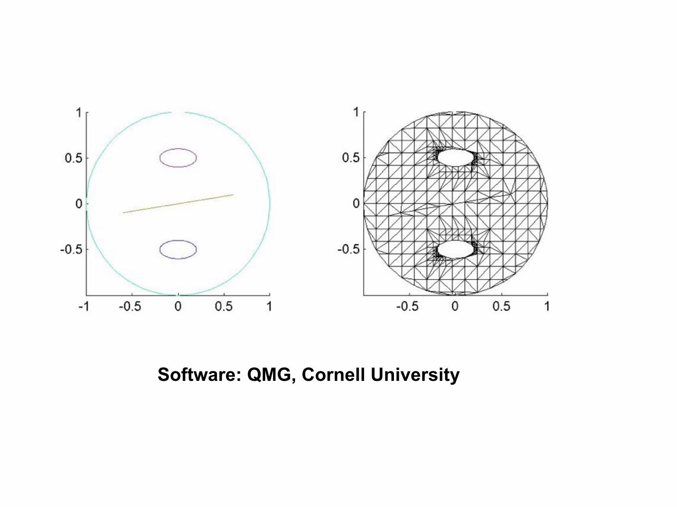
Software: QMG, Cornell University

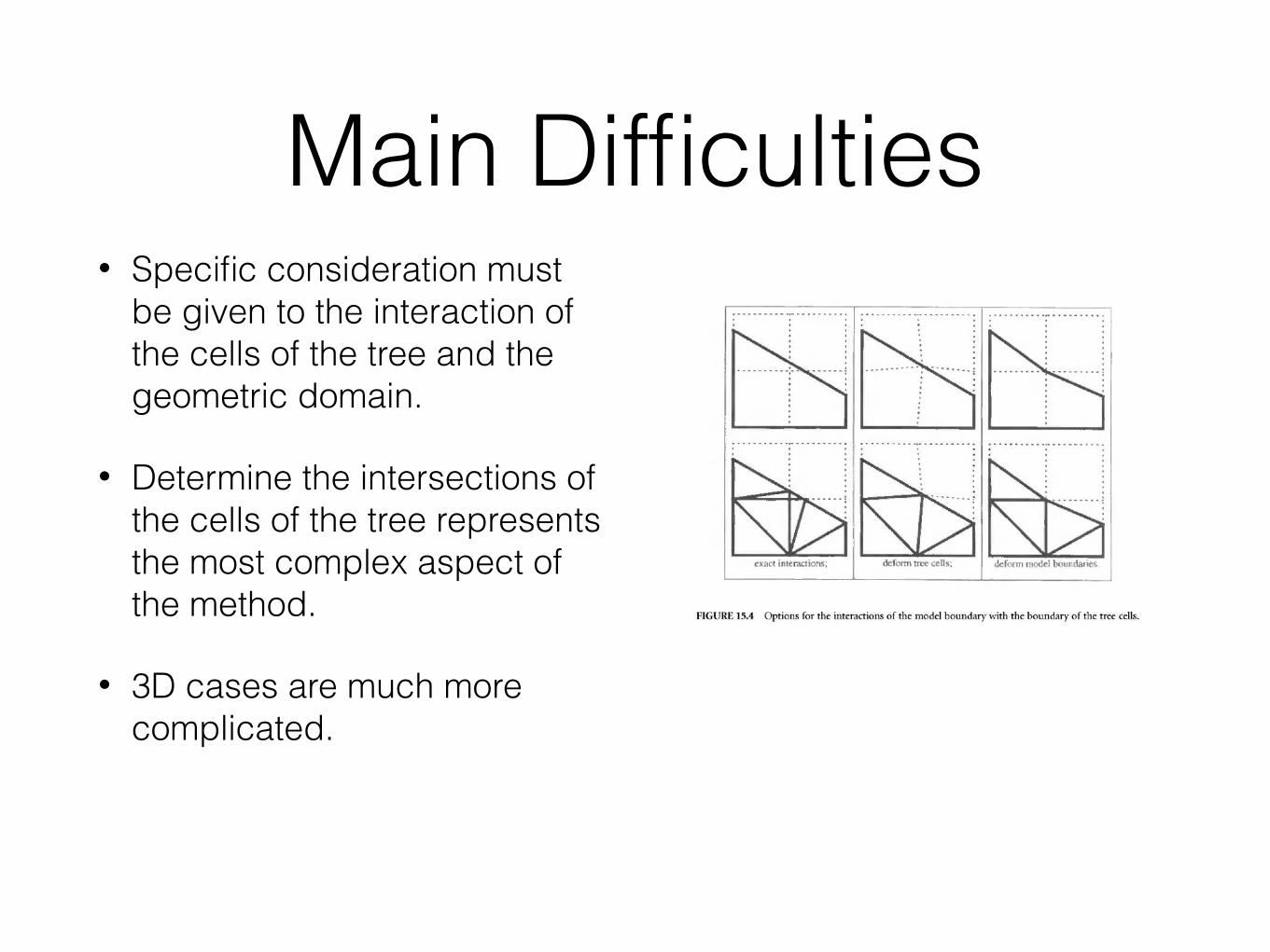
Main Difficulties• Specific consideration must

be given to the interaction of the cells of the tree and the geometric domain.

• Determine the intersections of the cells of the tree represents the most complex aspect of the method.

• 3D cases are much more complicated.

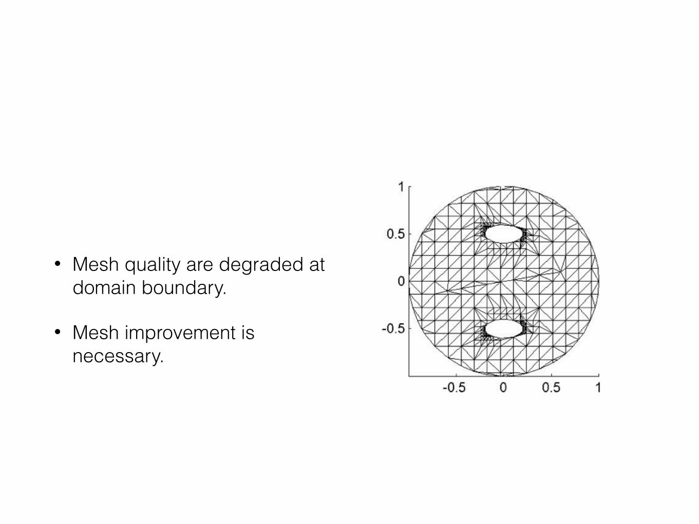
• Mesh quality are degraded at domain boundary.

• Mesh improvement is necessary.

Advancing Front

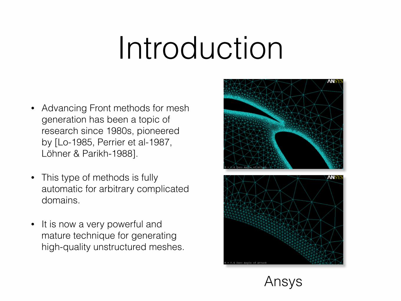
Introduction• Advancing Front methods for mesh

generation has been a topic of research since 1980s, pioneered by [Lo-1985, Perrier et al-1987, Löhner & Parikh-1988].

• This type of methods is fully automatic for arbitrary complicated domains.

• It is now a very powerful and mature technique for generating high-quality unstructured meshes.

Ansys

Introduction (cont’d)

• This method allows for the generation of high quality (aspect ratio) mesh elements that fit domain boundary.

• Mesh sizing control is easily adapted by using mesh spacing control functions. Resulting nicely graded meshes.

• On the other hand, convergence problems can occur, especially in 3d, as it is not always guarantee how to cover the entire domain.

General Principles

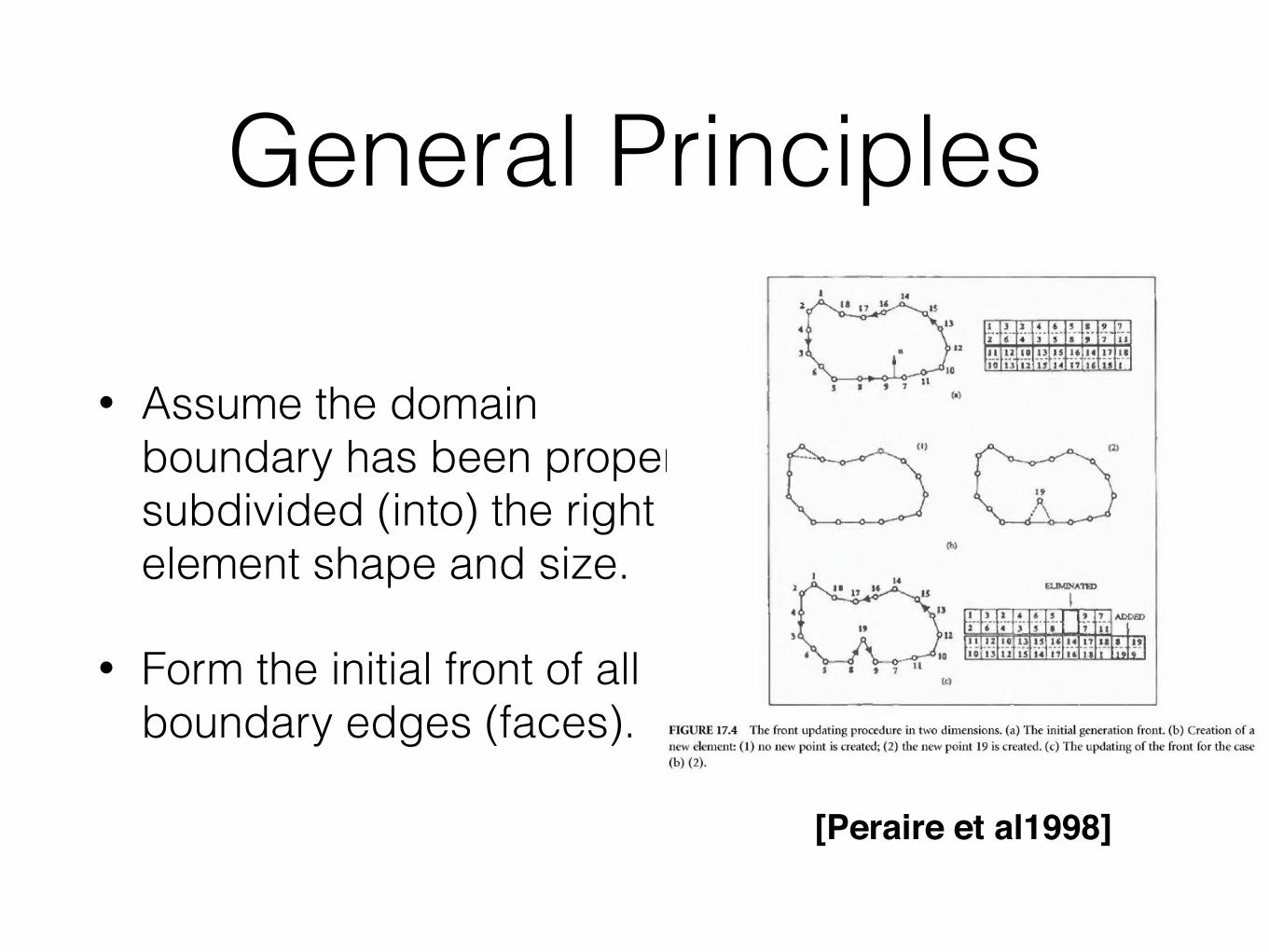
• Assume the domain boundary has been properly subdivided (into) the right element shape and size.

• Form the initial front of all boundary edges (faces).

[Peraire et al1998]

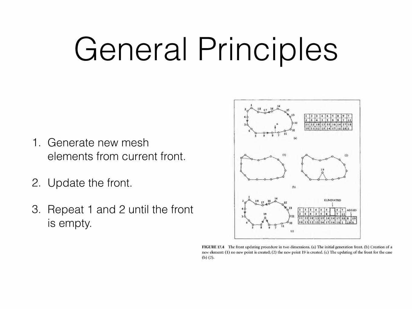
1. Generate new mesh elements from current front.

2. Update the front.

3. Repeat 1 and 2 until the front is empty.

General Principles

Advancing Front

A B

C

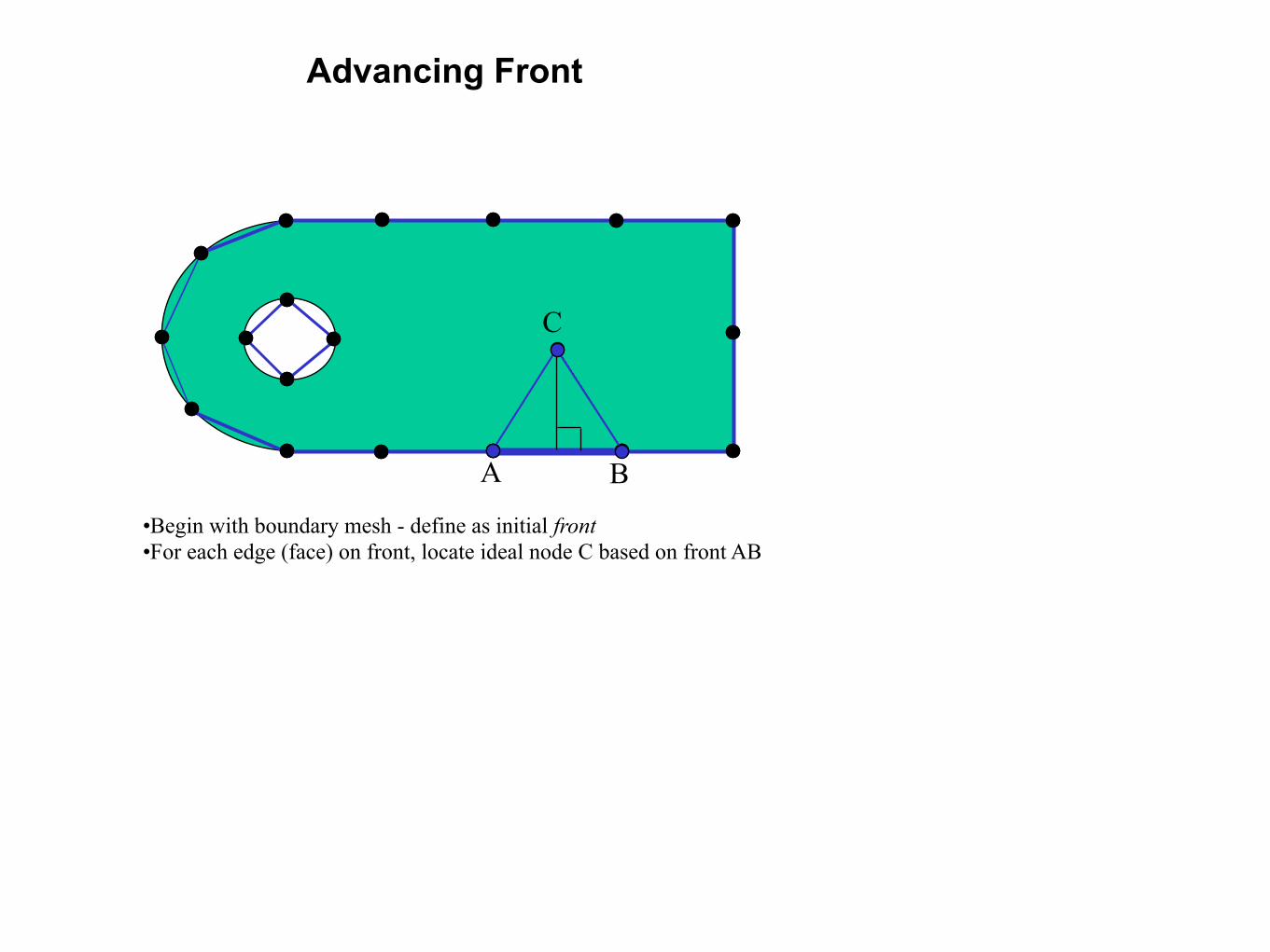
•Begin with boundary mesh - define as initial front •For each edge (face) on front, locate ideal node C based on front AB

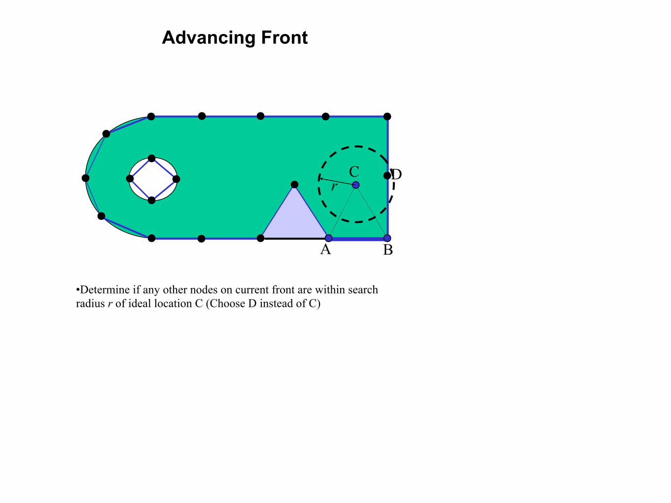
Advancing Front

A B

Cr

•Determine if any other nodes on current front are within search radius r of ideal location C (Choose D instead of C)

D

Advancing Front

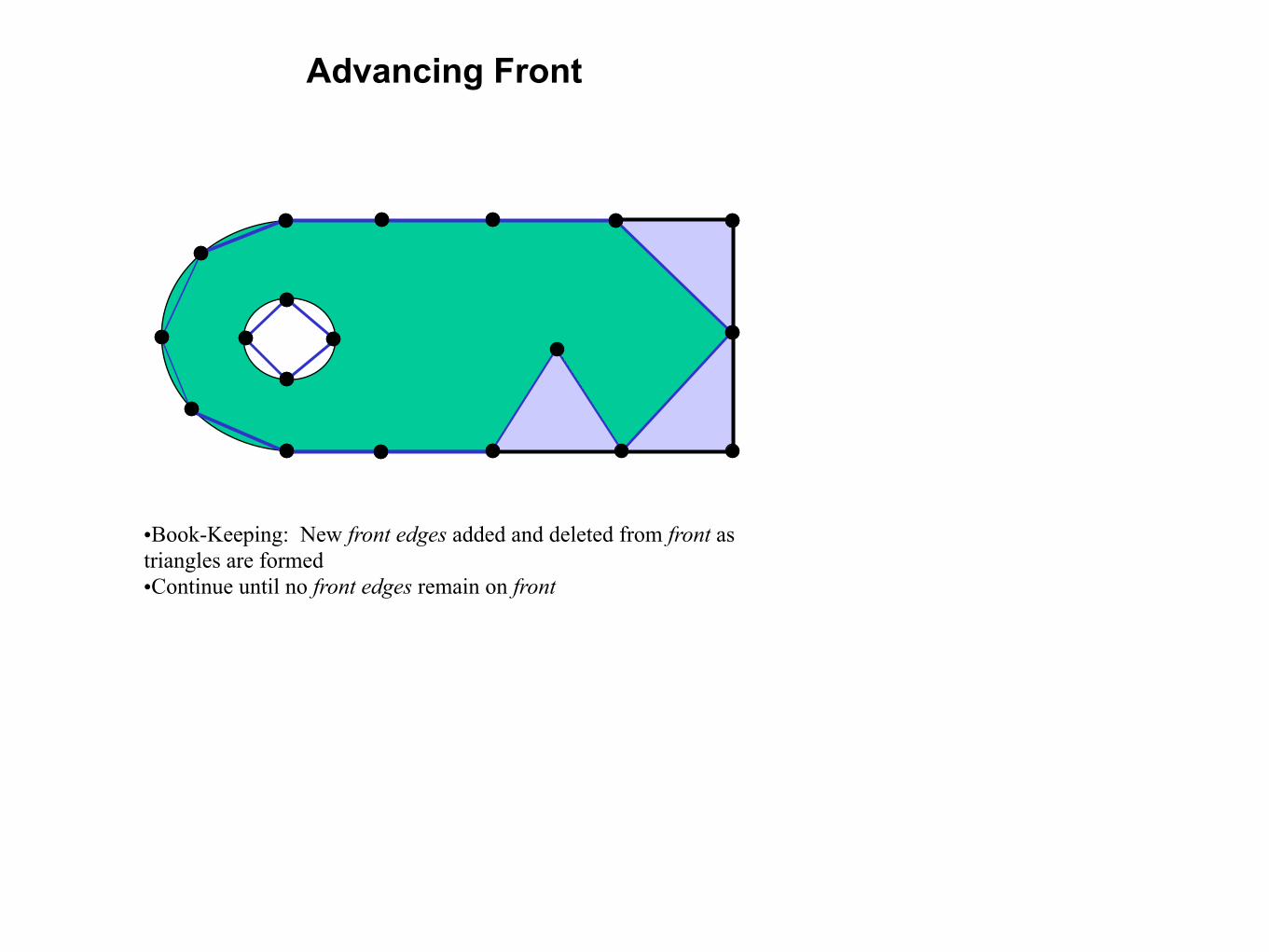
•Book-Keeping: New front edges added and deleted from front as triangles are formed •Continue until no front edges remain on front

D

Advancing Front

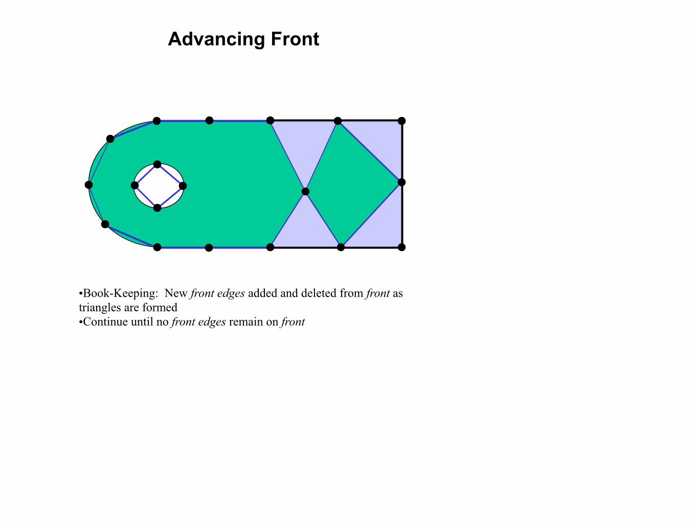
•Book-Keeping: New front edges added and deleted from front as triangles are formed •Continue until no front edges remain on front

Advancing Front

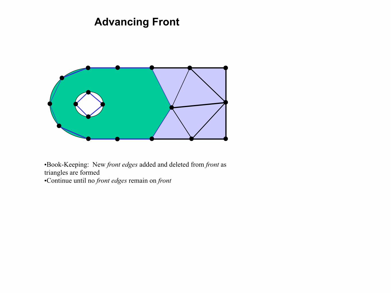
•Book-Keeping: New front edges added and deleted from front as triangles are formed •Continue until no front edges remain on front

Advancing Front

•Book-Keeping: New front edges added and deleted from front as triangles are formed •Continue until no front edges remain on front

Advancing Front

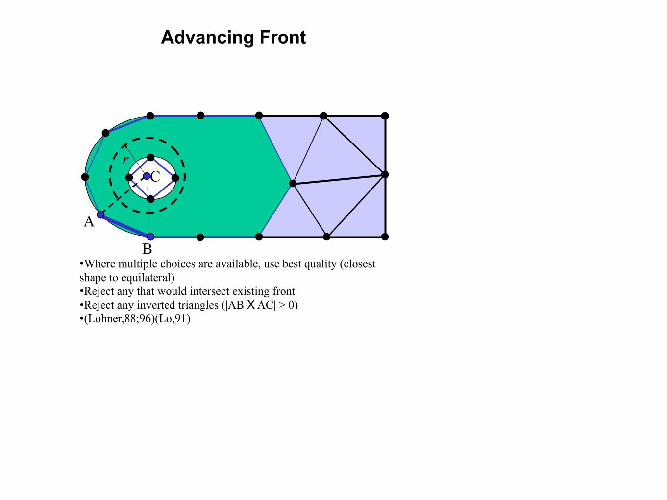
A

B

C

•Where multiple choices are available, use best quality (closest shape to equilateral) •Reject any that would intersect existing front •Reject any inverted triangles (|AB X AC| > 0) •(Lohner,88;96)(Lo,91)

r

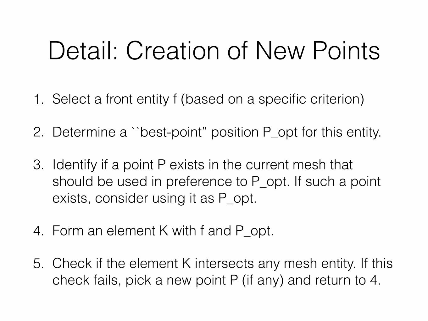
Detail: Creation of New Points1. Select a front entity f (based on a specific criterion)

2. Determine a ``best-point” position P_opt for this entity.

3. Identify if a point P exists in the current mesh that should be used in preference to P_opt. If such a point exists, consider using it as P_opt.

4. Form an element K with f and P_opt.

5. Check if the element K intersects any mesh entity. If this check fails, pick a new point P (if any) and return to 4.

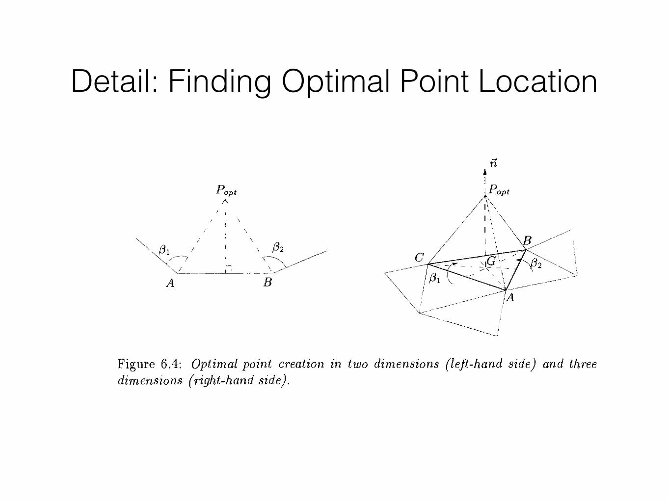
Detail: Finding Optimal Point Location

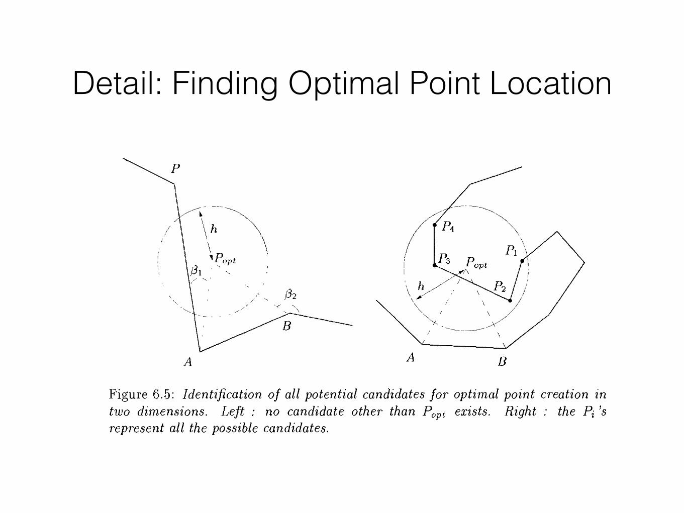
Detail: Finding Optimal Point Location

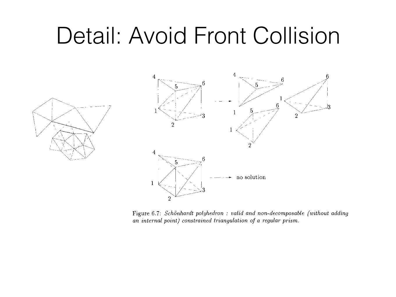
Detail: Avoid Front Collision

Remarks

• The principle of any AFT method is relatively simple and practical. It generates high quality meshes.

• However, several details to be implemented are all based on heuristics.

• In 3d, none of the AFT methods has guarantee that it will complete.

Delaunay-based Methods

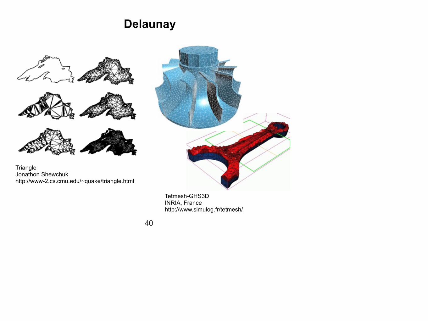
40

Delaunay

Triangle Jonathon Shewchuk http://www-2.cs.cmu.edu/~quake/triangle.html

Tetmesh-GHS3D INRIA, France http://www.simulog.fr/tetmesh/

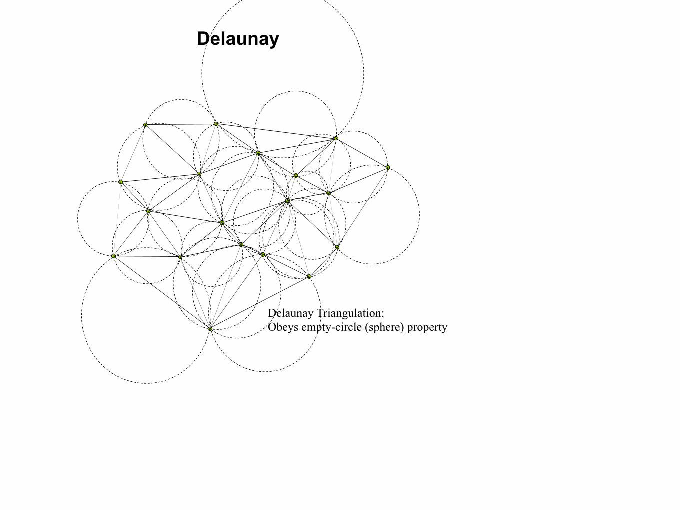
Delaunay Triangulation: Obeys empty-circle (sphere) property

Delaunay

Non-Delaunay Triangulation

Delaunay

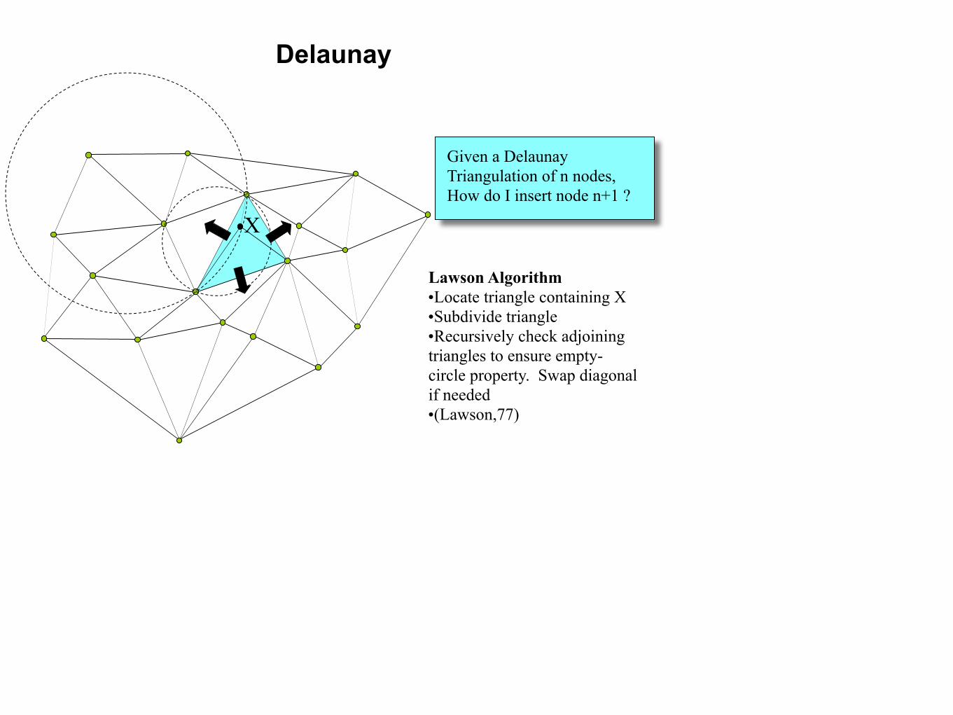
Lawson Algorithm •Locate triangle containing X •Subdivide triangle •Recursively check adjoining triangles to ensure empty-circle property. Swap diagonal if needed •(Lawson,77)

X

Given a Delaunay Triangulation of n nodes, How do I insert node n+1 ?

Delaunay

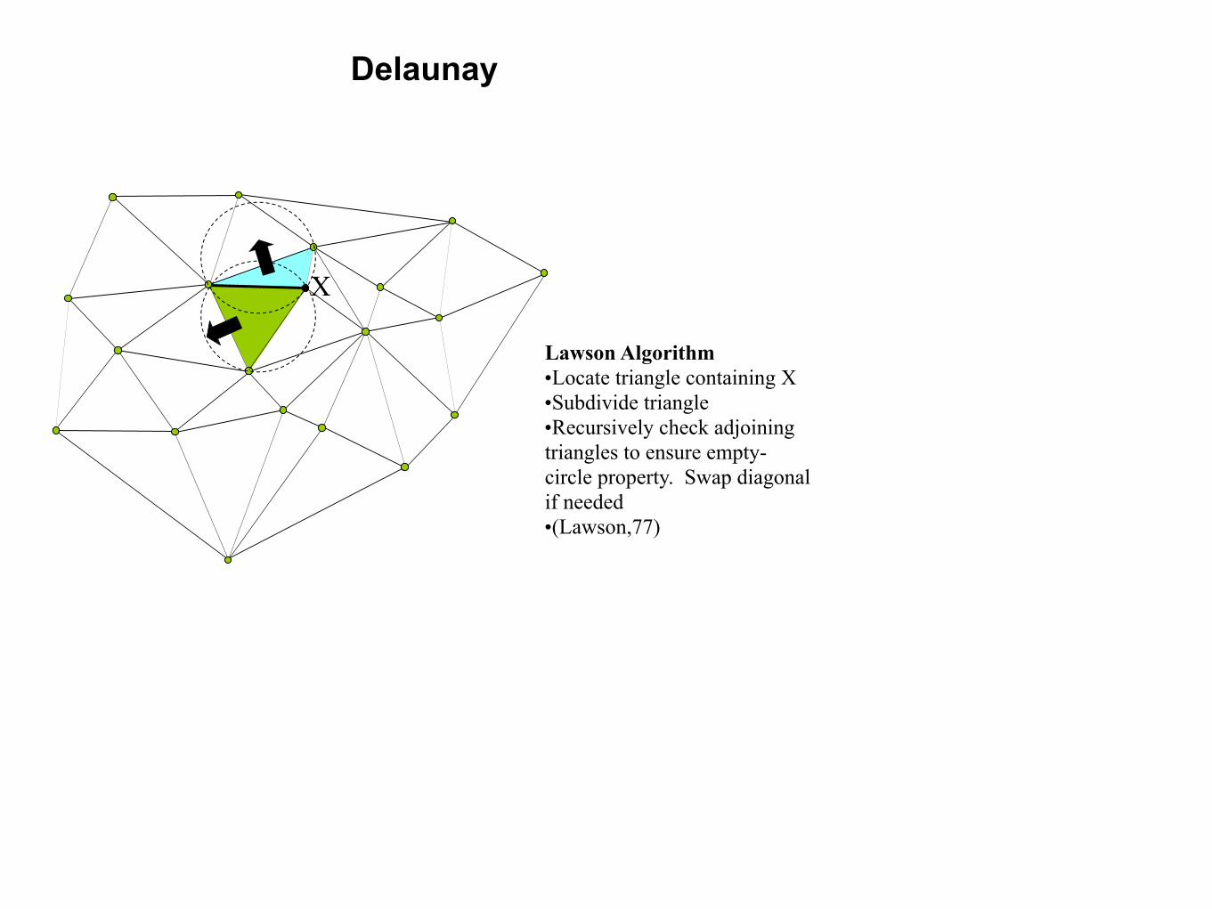
X

Lawson Algorithm •Locate triangle containing X •Subdivide triangle •Recursively check adjoining triangles to ensure empty-circle property. Swap diagonal if needed •(Lawson,77)

Delaunay

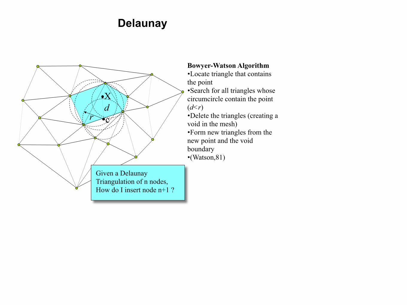
Bowyer-Watson Algorithm •Locate triangle that contains the point •Search for all triangles whose circumcircle contain the point (d<r) •Delete the triangles (creating a void in the mesh) •Form new triangles from the new point and the void boundary •(Watson,81)

X

r cd

Given a Delaunay Triangulation of n nodes, How do I insert node n+1 ?

Delaunay

Delaunay

•Begin with Bounding Triangles (or Tetrahedra)

Delaunay

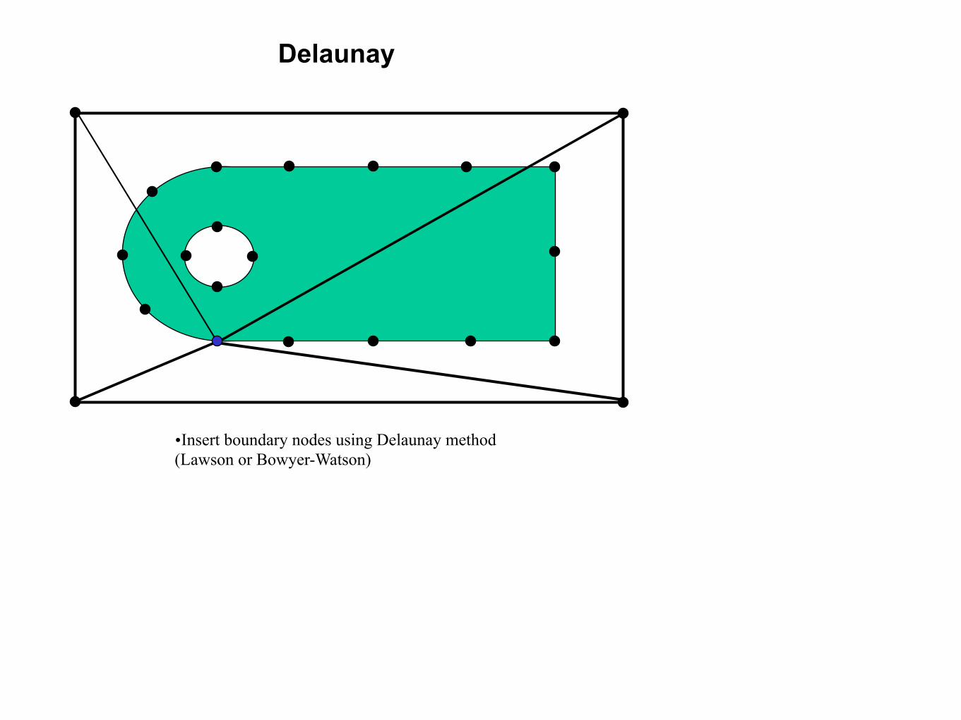
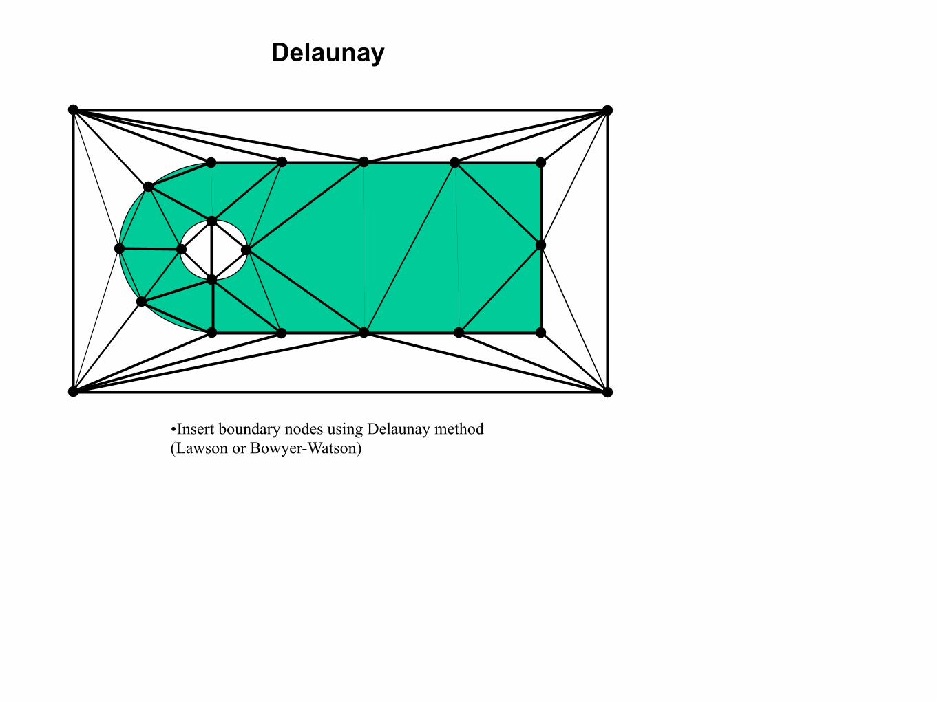
•Insert boundary nodes using Delaunay method (Lawson or Bowyer-Watson)

Delaunay

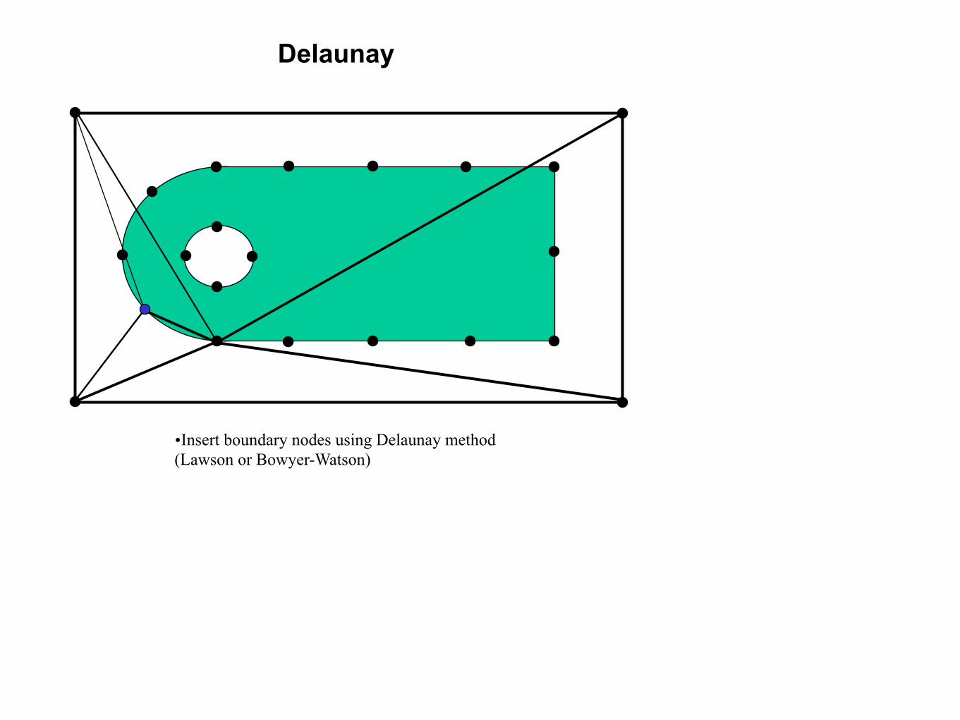
•Insert boundary nodes using Delaunay method (Lawson or Bowyer-Watson)

Delaunay

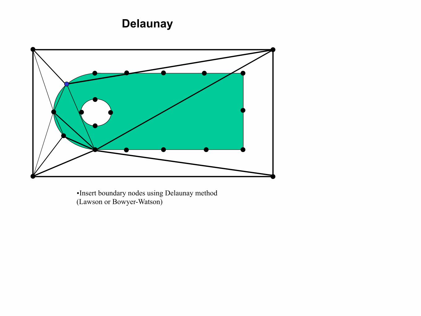
•Insert boundary nodes using Delaunay method (Lawson or Bowyer-Watson)

Delaunay

•Insert boundary nodes using Delaunay method (Lawson or Bowyer-Watson)

Delaunay

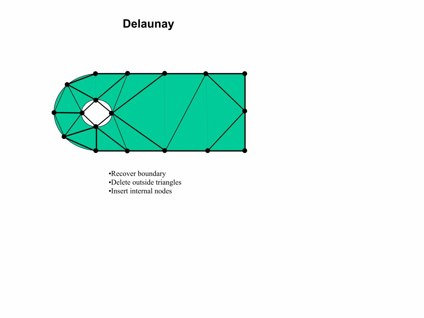
•Recover boundary •Delete outside triangles •Insert internal nodes

Delaunay

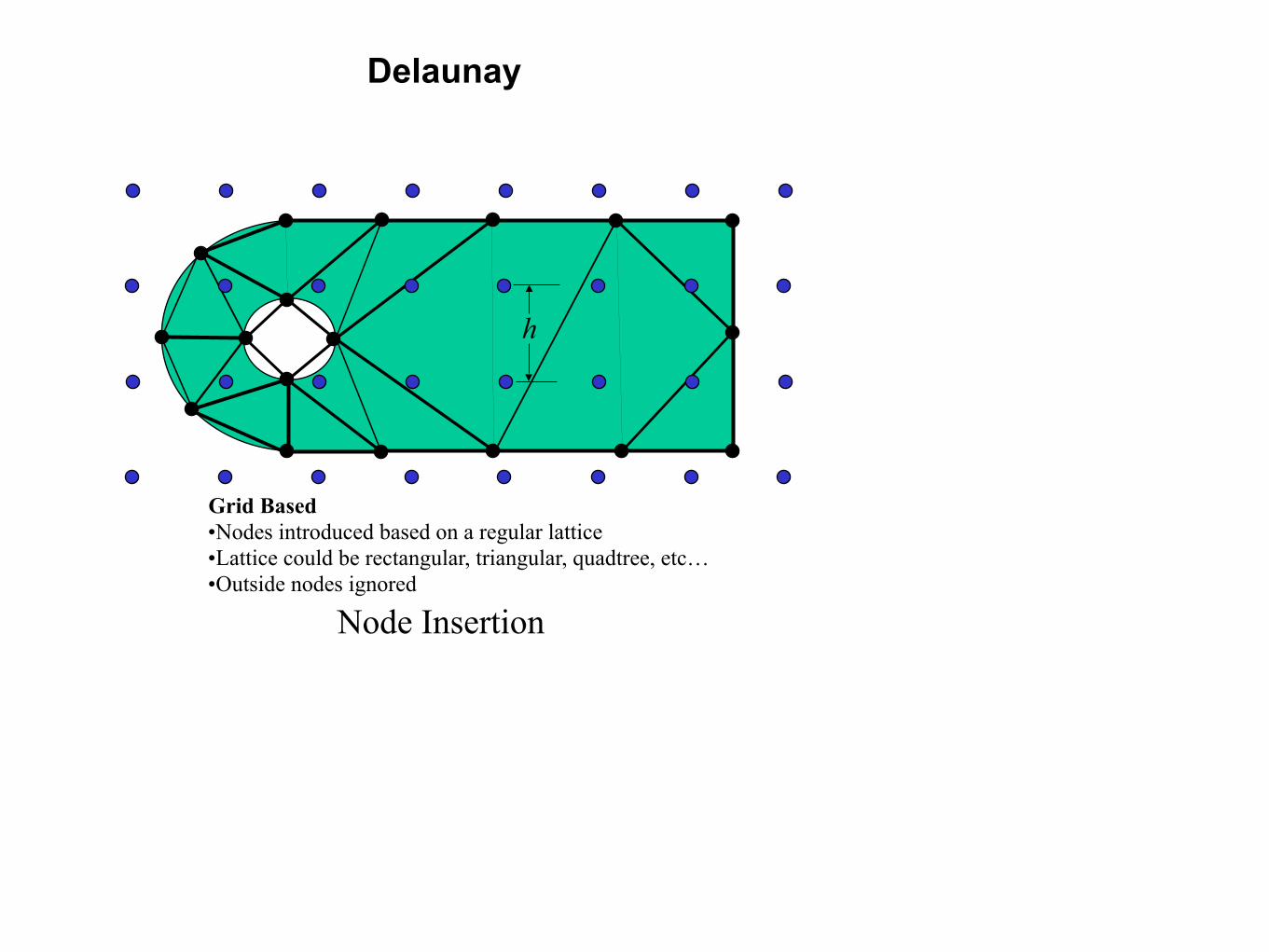
Node Insertion

Grid Based •Nodes introduced based on a regular lattice •Lattice could be rectangular, triangular, quadtree, etc… •Outside nodes ignored

h

Delaunay

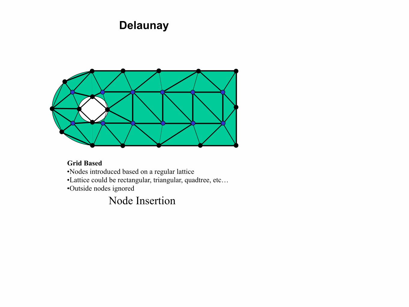
Node Insertion

Grid Based •Nodes introduced based on a regular lattice •Lattice could be rectangular, triangular, quadtree, etc… •Outside nodes ignored

Delaunay

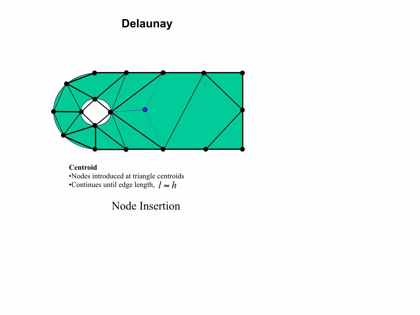
Node Insertion

Centroid •Nodes introduced at triangle centroids •Continues until edge length, hl ≈

Delaunay

Node Insertion

Centroid •Nodes introduced at triangle centroids •Continues until edge length, hl ≈

l

Delaunay

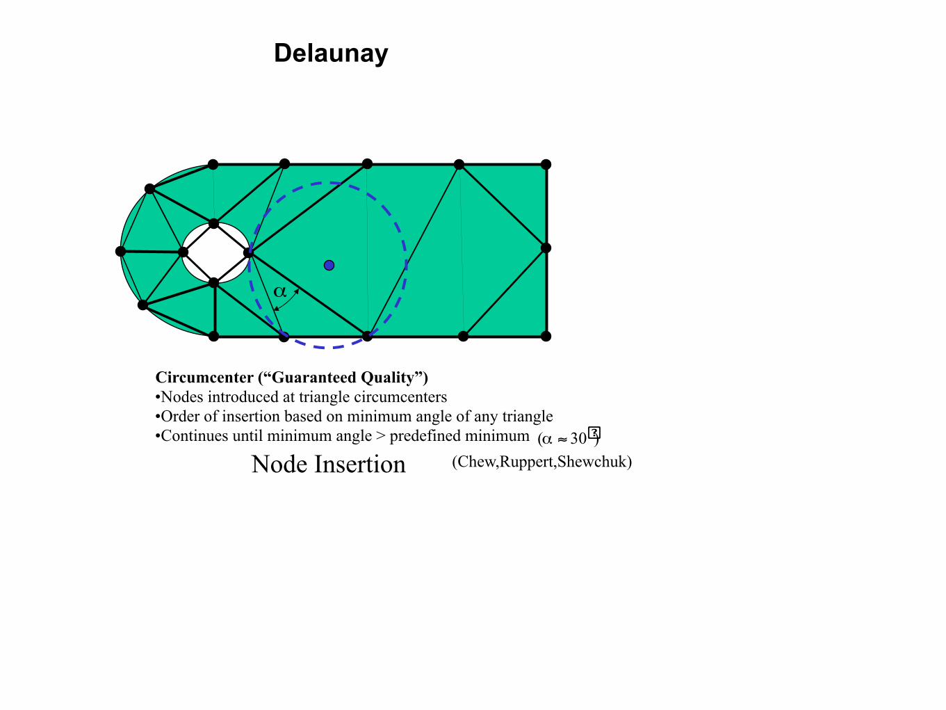
Node Insertion

Circumcenter (“Guaranteed Quality”) •Nodes introduced at triangle circumcenters •Order of insertion based on minimum angle of any triangle •Continues until minimum angle > predefined minimum

α

)30( �≈α(Chew,Ruppert,Shewchuk)

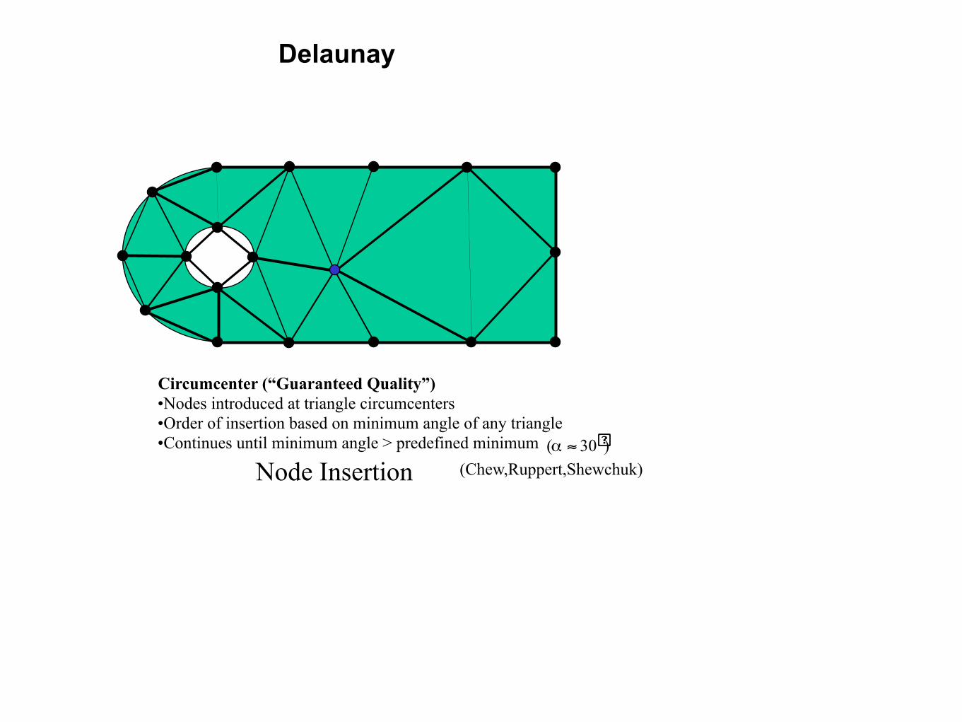
Delaunay

Circumcenter (“Guaranteed Quality”) •Nodes introduced at triangle circumcenters •Order of insertion based on minimum angle of any triangle •Continues until minimum angle > predefined minimum )30( �≈α

Node Insertion (Chew,Ruppert,Shewchuk)

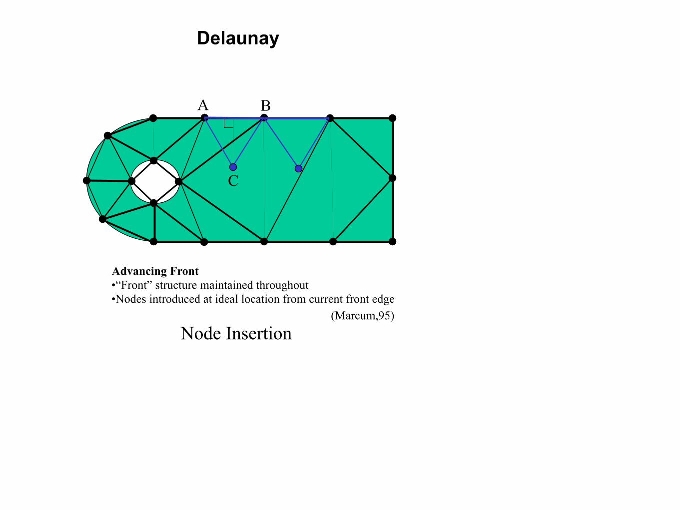
Delaunay

Advancing Front •“Front” structure maintained throughout •Nodes introduced at ideal location from current front edge

Node Insertion

A B

C

(Marcum,95)

Delaunay

Advancing Front •“Front” structure maintained throughout •Nodes introduced at ideal location from current front edge

Node Insertion(Marcum,95)

Delaunay

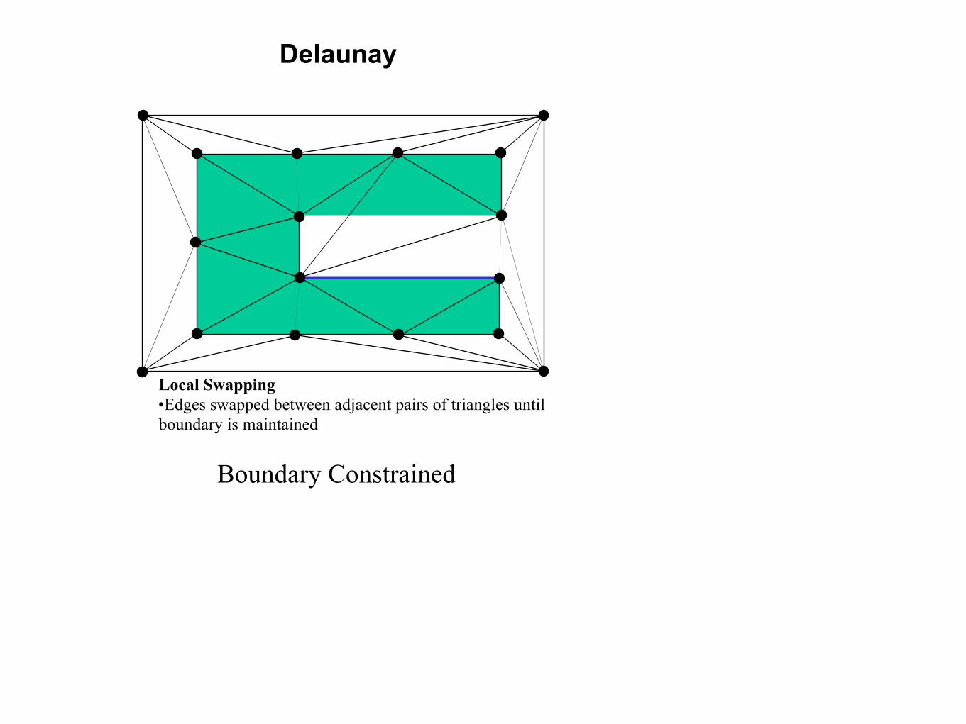
Boundary Constrained

Local Swapping •Edges swapped between adjacent pairs of triangles until boundary is maintained

Delaunay

Boundary Constrained

Local Swapping •Edges swapped between adjacent pairs of triangles until boundary is maintained

Delaunay

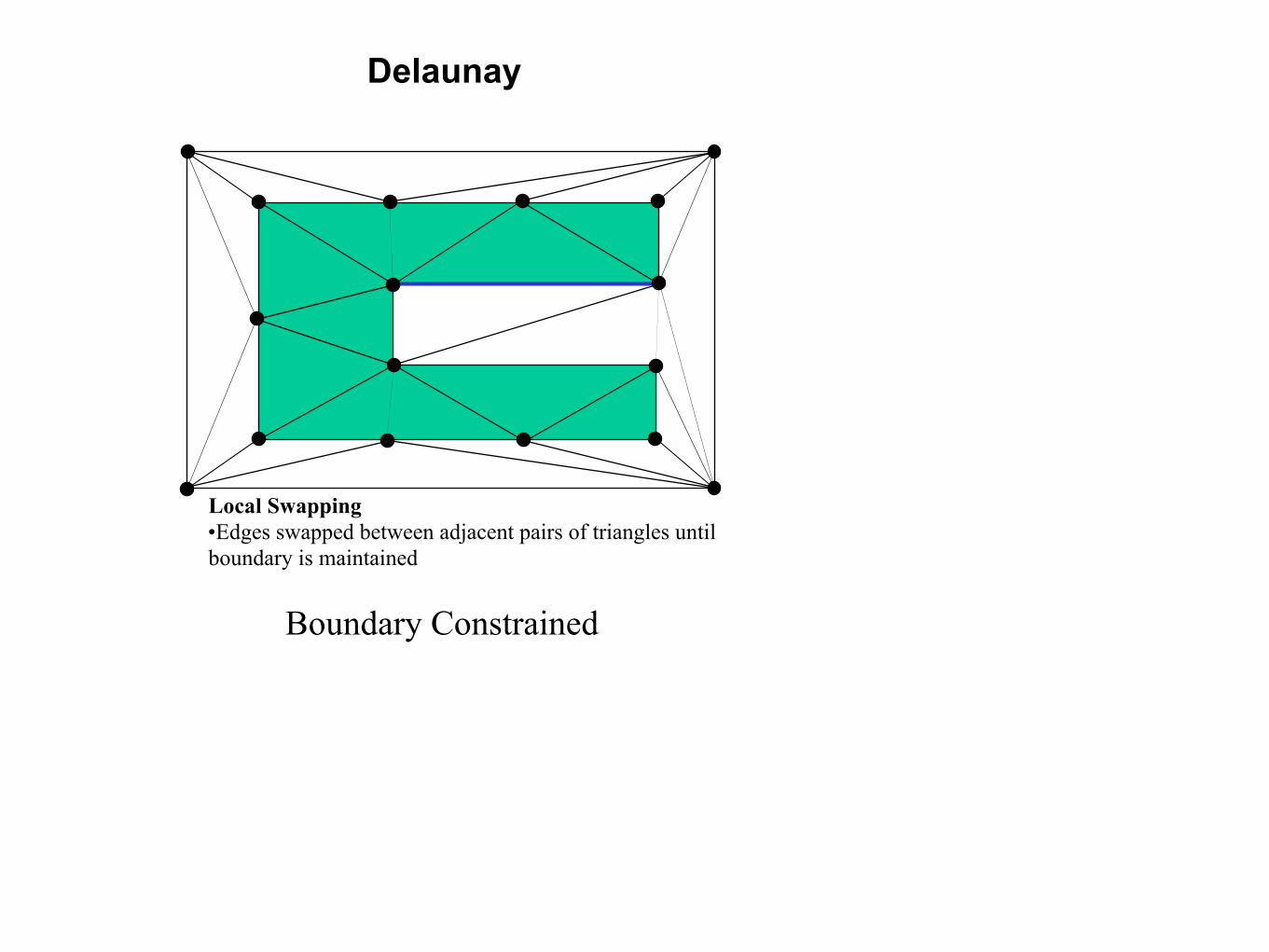
Boundary Constrained

Local Swapping •Edges swapped between adjacent pairs of triangles until boundary is maintained

Delaunay

Boundary Constrained

Local Swapping •Edges swapped between adjacent pairs of triangles until boundary is maintained

Delaunay

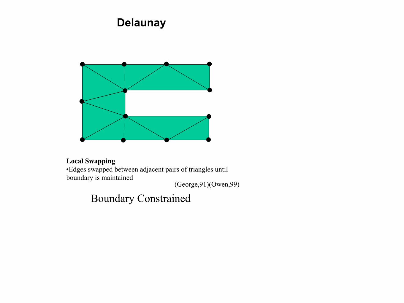
Boundary Constrained

Local Swapping •Edges swapped between adjacent pairs of triangles until boundary is maintained

(George,91)(Owen,99)

D C

VS

Delaunay

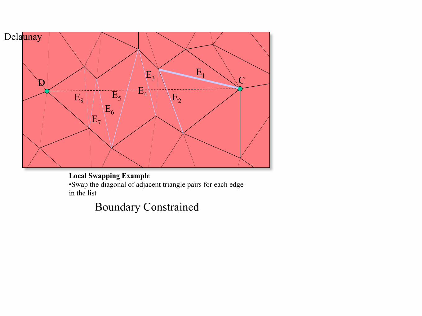
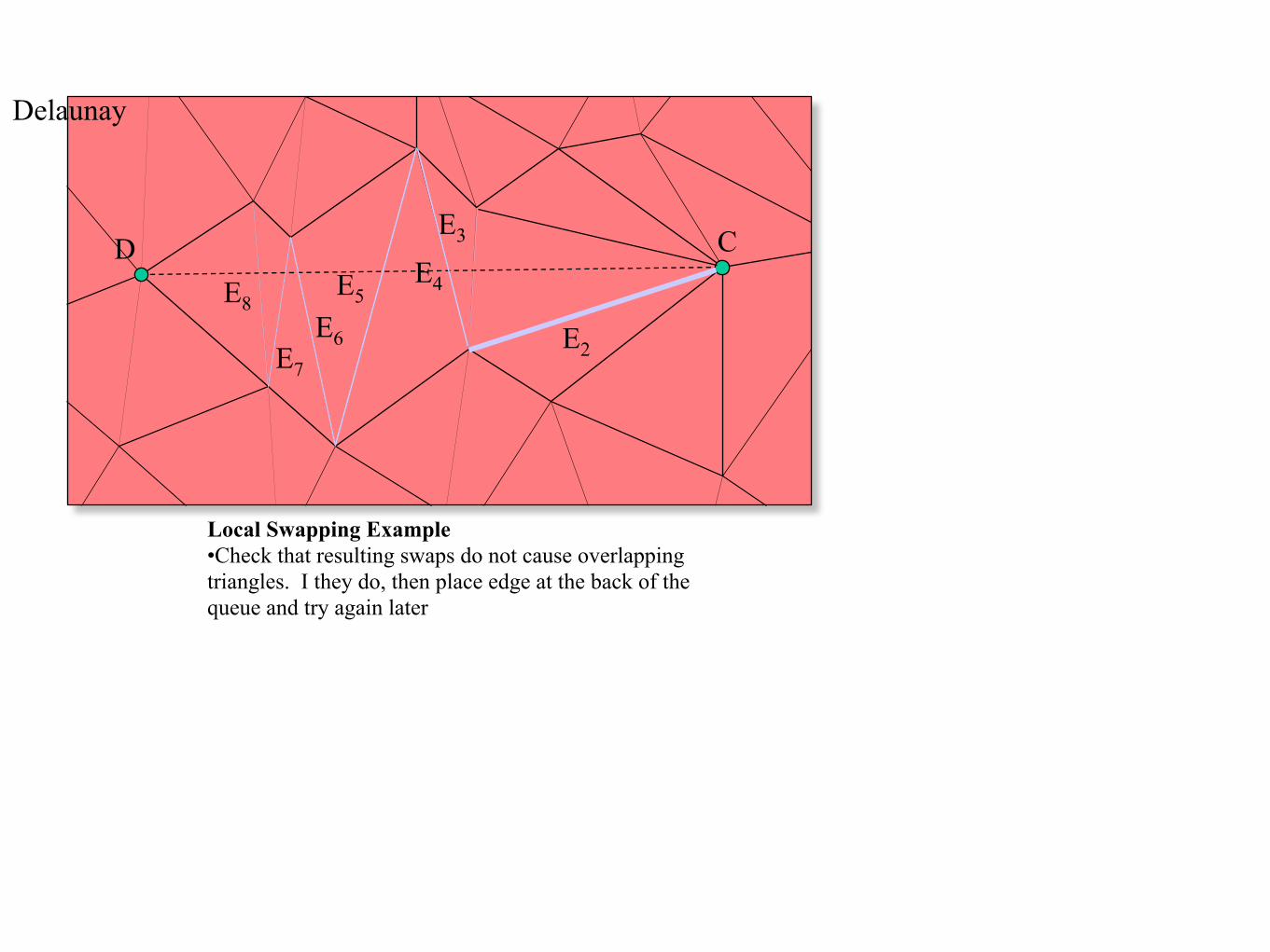
Local Swapping Example •Recover edge CD at vector Vs

Boundary Constrained

D C

E1

E2

E3

E4E5

E6E7

E8

Local Swapping Example •Make a list (queue) of all edges Ei, that intersect Vs

Delaunay

Boundary Constrained

D CE1

E2

E3

E4E5

E6E7

E8

Delaunay

Local Swapping Example •Swap the diagonal of adjacent triangle pairs for each edge in the list

Boundary Constrained

D C

E2

E3

E4E5

E6E7

E8

Delaunay

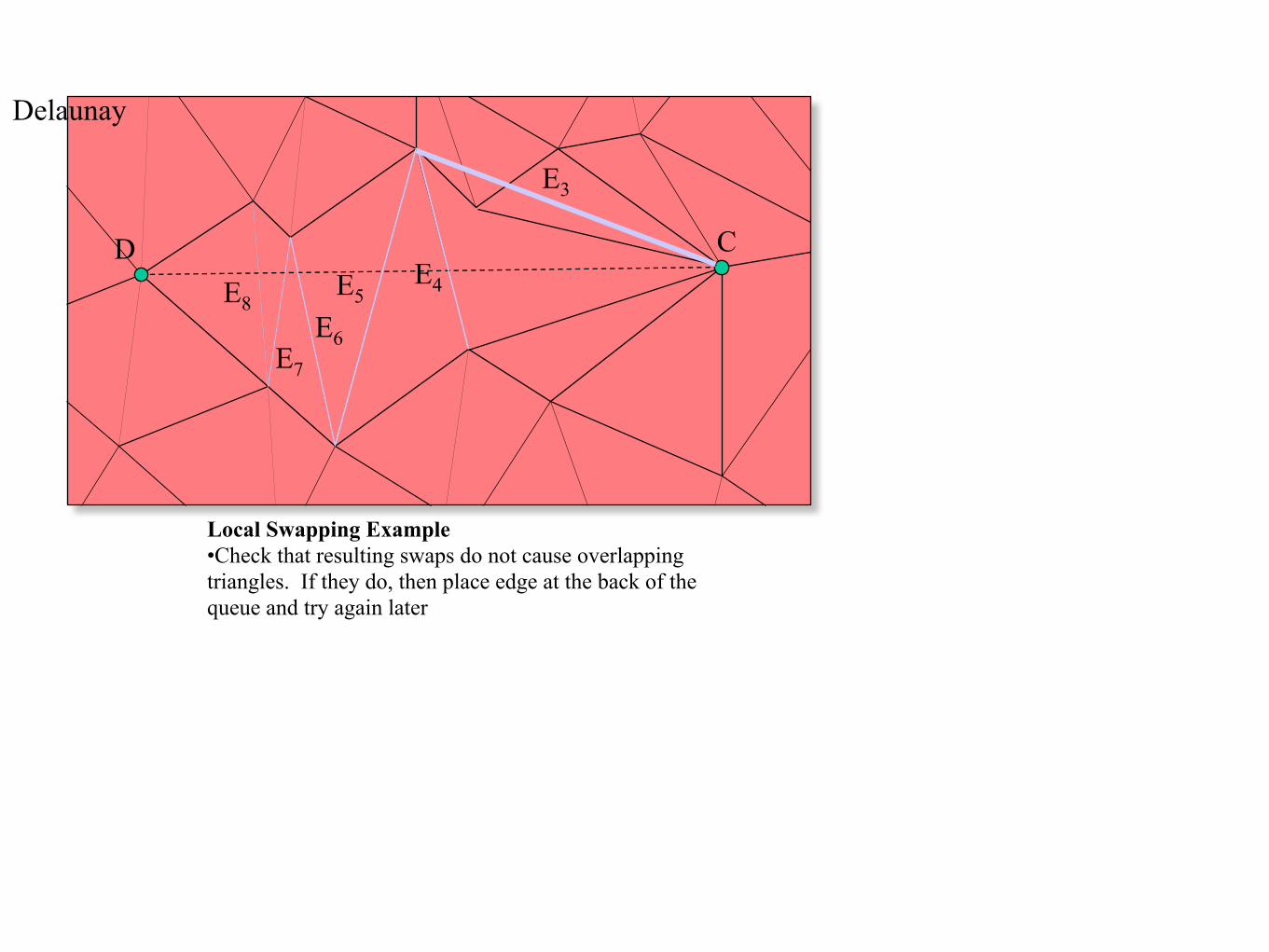
Local Swapping Example •Check that resulting swaps do not cause overlapping triangles. I they do, then place edge at the back of the queue and try again later

D C

E3

E4E5

E6E7

E8

Delaunay

Local Swapping Example •Check that resulting swaps do not cause overlapping triangles. If they do, then place edge at the back of the queue and try again later

D C

E6

Local Swapping Example •Final swap will recover the desired edge. •Resulting triangle quality may be poor if multiple swaps were necessary •Does not maintain Delaunay criterion!

Delaunay

A

C

D E

B

Boundary Constrained

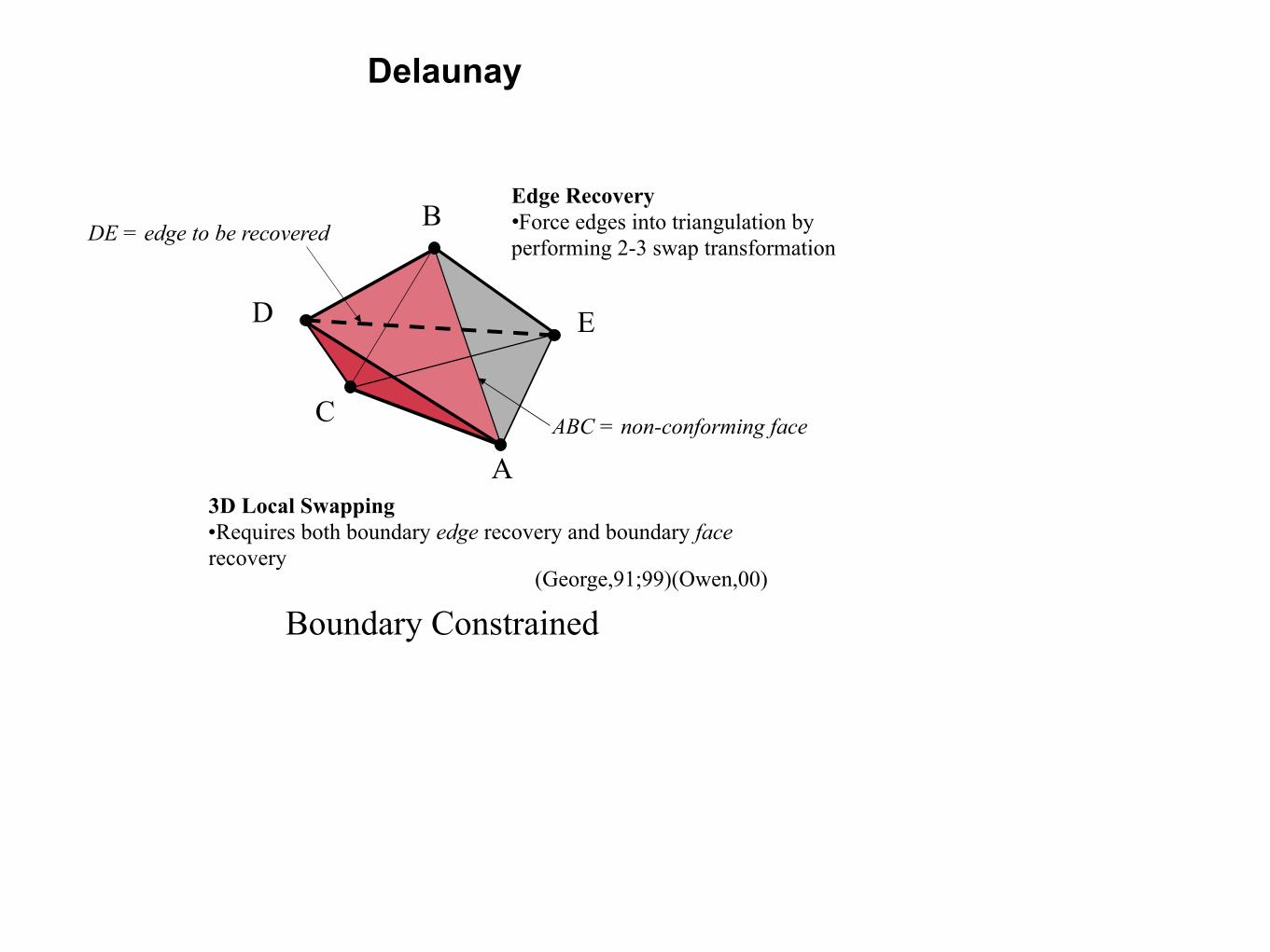
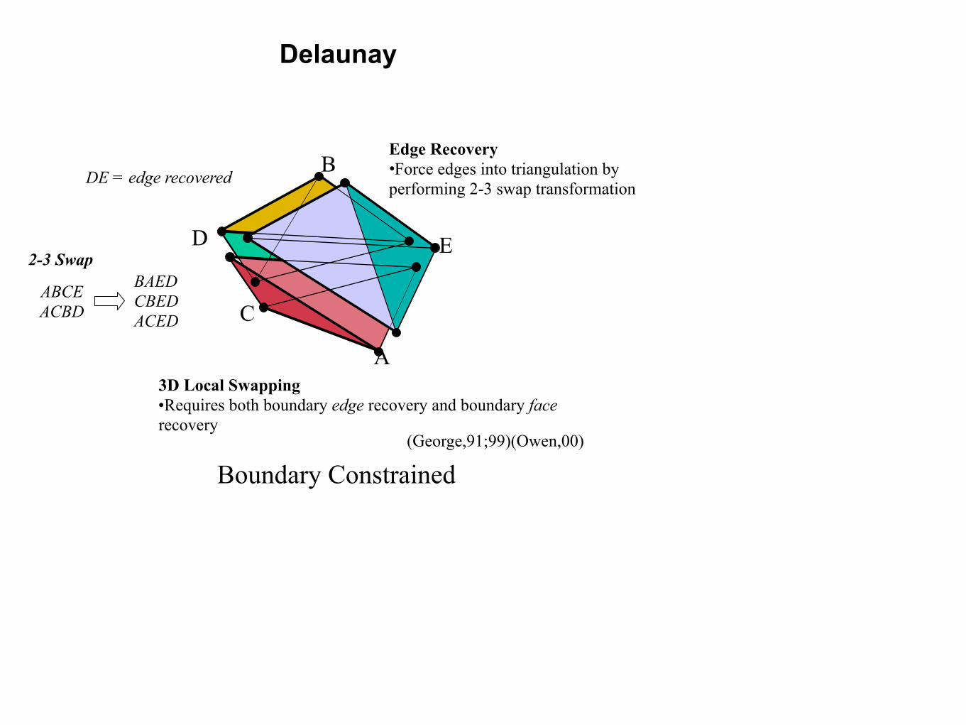
3D Local Swapping •Requires both boundary edge recovery and boundary face recovery

Edge Recovery •Force edges into triangulation by performing 2-3 swap transformation

ABC = non-conforming face

DE = edge to be recovered

(George,91;99)(Owen,00)

Delaunay

A

B

C

D E

Boundary Constrained

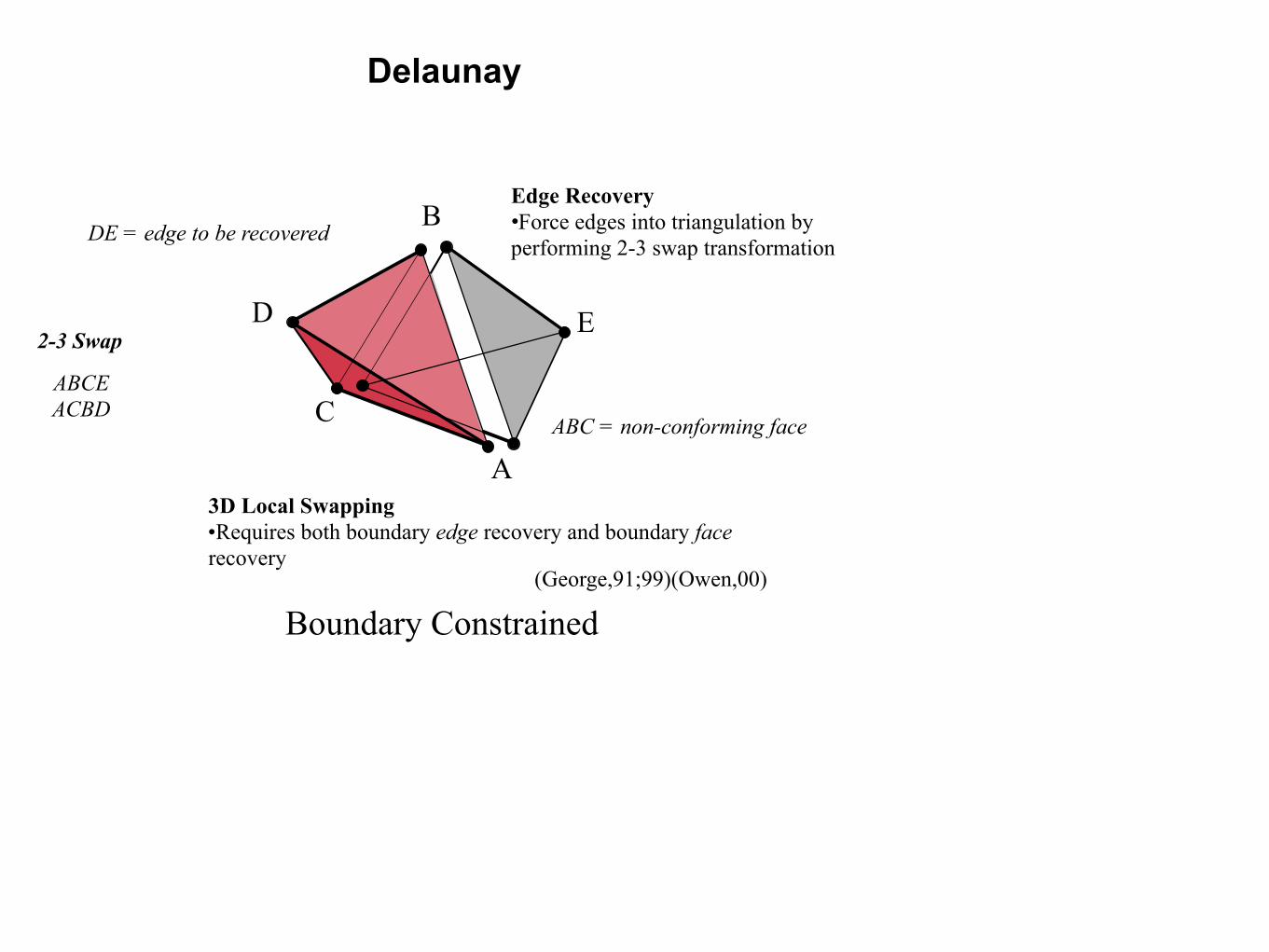
3D Local Swapping •Requires both boundary edge recovery and boundary face recovery

Edge Recovery •Force edges into triangulation by performing 2-3 swap transformation

ABC = non-conforming face

DE = edge to be recovered

ABCE ACBD

2-3 Swap

(George,91;99)(Owen,00)

Delaunay

A

B

C

D E

Boundary Constrained

3D Local Swapping •Requires both boundary edge recovery and boundary face recovery

Edge Recovery •Force edges into triangulation by performing 2-3 swap transformation

ABCE ACBD

2-3 SwapBAED CBED ACED

DE = edge recovered

(George,91;99)(Owen,00)

Delaunay

A

C

D E

B

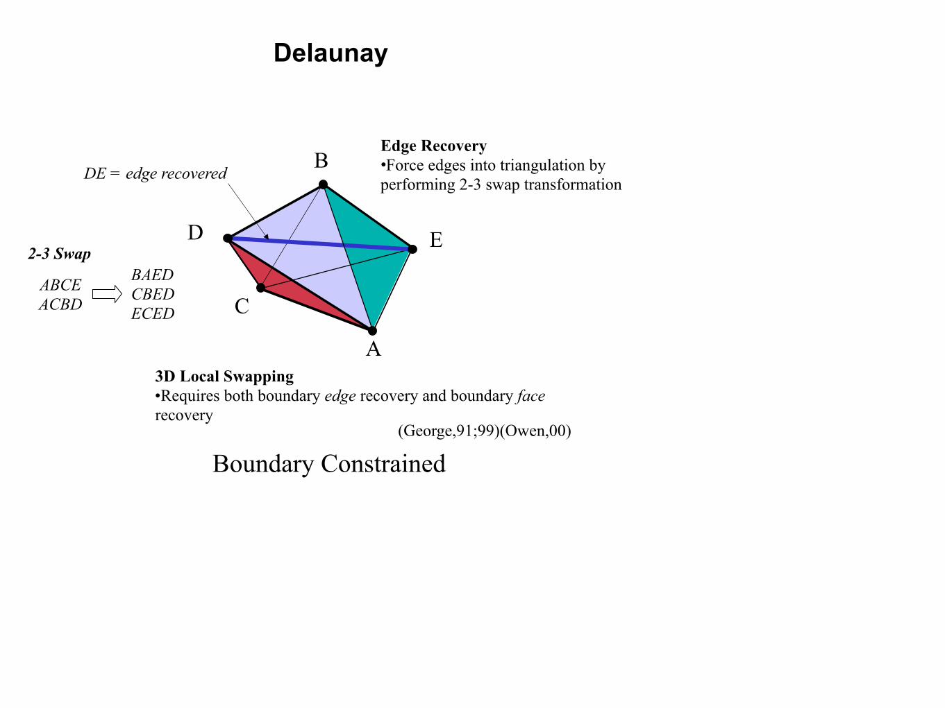
Boundary Constrained

3D Local Swapping •Requires both boundary edge recovery and boundary face recovery

Edge Recovery •Force edges into triangulation by performing 2-3 swap transformation

DE = edge recovered

ABCE ACBD

2-3 SwapBAED CBED ECED

(George,91;99)(Owen,00)

Delaunay

A B

A BS

S

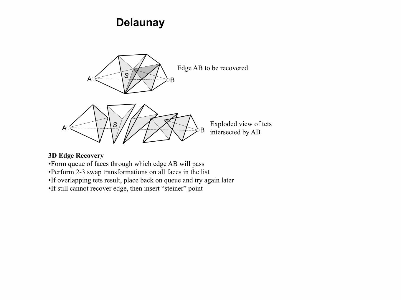
3D Edge Recovery •Form queue of faces through which edge AB will pass •Perform 2-3 swap transformations on all faces in the list •If overlapping tets result, place back on queue and try again later •If still cannot recover edge, then insert “steiner” point

Edge AB to be recovered

Exploded view of tets intersected by AB