Embed Size (px)
Citation preview
Overview of Tuesday, April 21 Overview of Tuesday, April 21 discussion: Option valuation discussion: Option valuation principles & intro to binomial modelprinciples & intro to binomial model
FIN 441FIN 441
Prof. RogersProf. Rogers
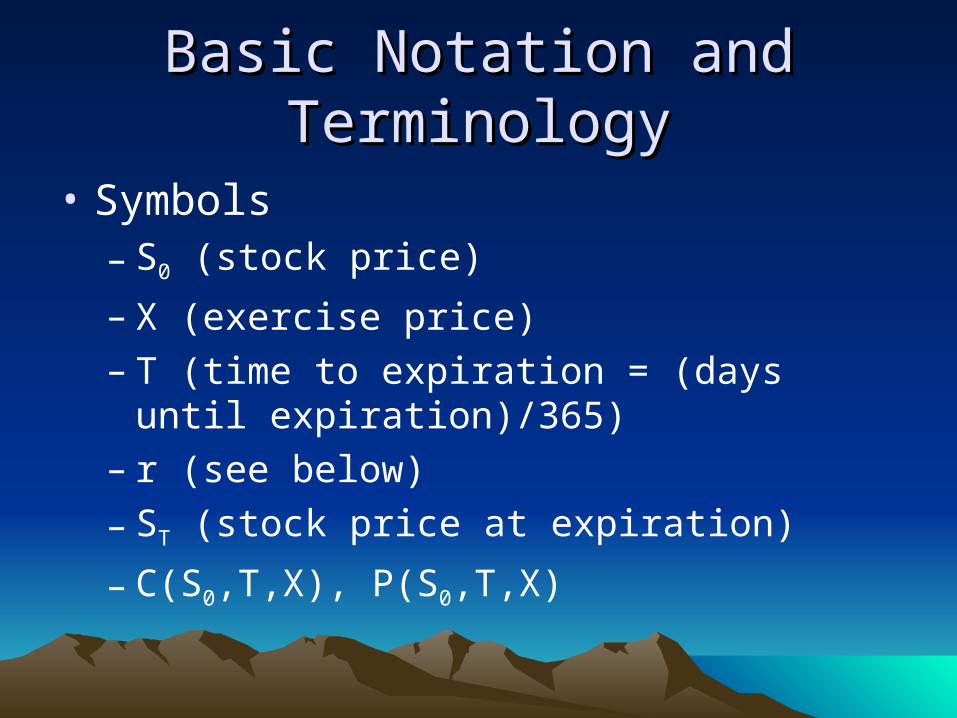
Basic Notation and TerminologyBasic Notation and Terminology
• Symbols– S0 (stock price)
– X (exercise price)– T (time to expiration = (days until
expiration)/365)– r (see below)
– ST (stock price at expiration)
– C(S0,T,X), P(S0,T,X)
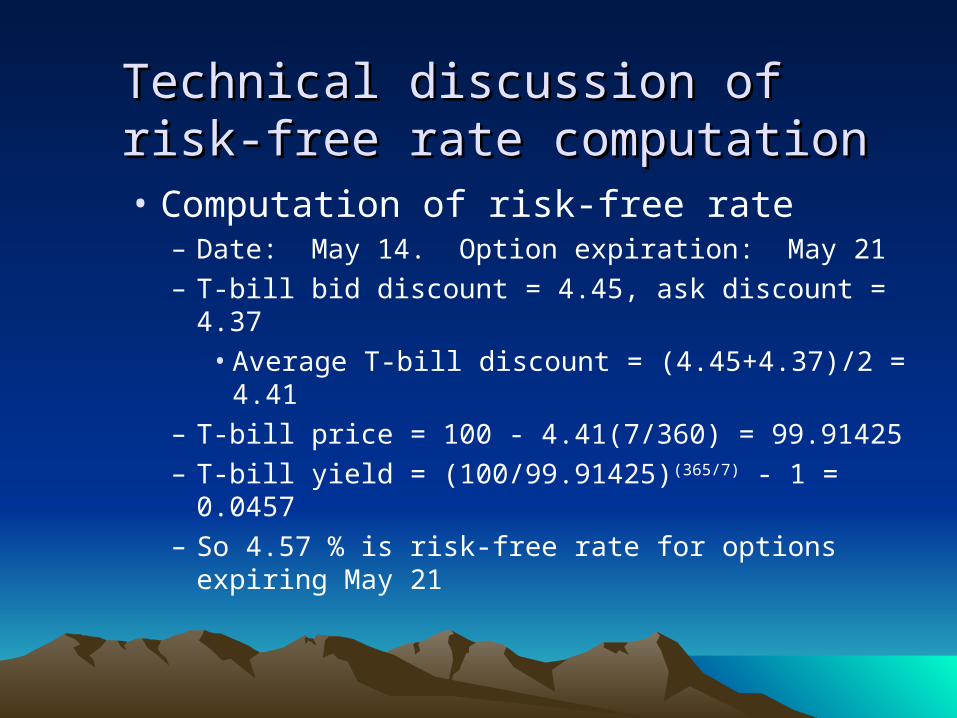
Technical discussion of risk-free rate Technical discussion of risk-free rate computationcomputation• Computation of risk-free rate
– Date: May 14. Option expiration: May 21– T-bill bid discount = 4.45, ask discount = 4.37
• Average T-bill discount = (4.45+4.37)/2 = 4.41– T-bill price = 100 - 4.41(7/360) = 99.91425– T-bill yield = (100/99.91425)(365/7) - 1 = 0.0457– So 4.57 % is risk-free rate for options expiring May
21
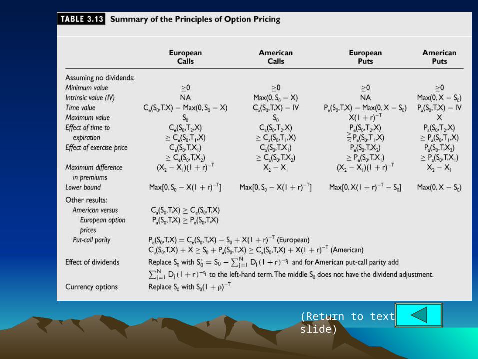
Principles of Call Option PricingPrinciples of Call Option Pricing
• Minimum Value of a Call– C(S0,T,X) 0 (for any call)
– For American calls:• Ca(S0,T,X) Max(0,S0 - X)
– Concept of intrinsic value: Max(0,S0 - X)
– Concept of time value of option• C(S,T,X) – Max(0,S – X)
Principles of Call Option Pricing Principles of Call Option Pricing (continued)(continued)
• Maximum Value of a Call– C(S0,T,X) S0
– “Right” but not “obligation” can never be more valuable than underlying asset (and will typically be worth less).
– Option values are always equal to a percentage of the underlying asset’s value!
Principles of Call Option Pricing Principles of Call Option Pricing (continued)(continued)
• Effect of Time to Expiration– More time until expiration, higher option
value!• Volatility is related to time (we’ll see this in
binomial and Black-Scholes models).• Calls allow buyer to invest in other assets, thus
a pure time value of money effect.
Principles of Call Option Pricing Principles of Call Option Pricing (continued)(continued)
• Effect of Exercise Price– Lower exercise prices on call options with
same underlying and time to expiration always have higher values!
Principles of Call Option Pricing Principles of Call Option Pricing (continued)(continued)
• Lower Bound of a European Call– Ce(S0,T,X) Max[0,S0 - X(1+r)-T]
– This is the lower bound for a European call
Principles of Call Option Pricing Principles of Call Option Pricing (continued)(continued)
• American Call Versus European Call– Ca(S0,T,X) Ce(S0,T,X)– If there are no dividends on the stock, an
American call will never be exercised early.– It will always be better to sell the call in the
market.– In such cases, the value of the American call
and identical European call should be equal.
Principles of Put Option PricingPrinciples of Put Option Pricing
• Minimum Value of a Put– P(S0,T,X) 0 (for any put)
– For American puts:• Pa(S0,T,X) Max(0,X - S0)
– Concept of intrinsic value: Max(0,X - S0)
Principles of Put Option Pricing Principles of Put Option Pricing (continued)(continued)
• Maximum Value of a Put– Pe(S0,T,X) X(1+r)-T
– Pa(S0,T,X) X
Principles of Put Option Pricing Principles of Put Option Pricing (continued)(continued)
• The Effect of Time to Expiration– Same effect as call options: more time, more
value!
Principles of Put Option Pricing Principles of Put Option Pricing (continued)(continued)
• Effect of Exercise Price– Raising exercise price of put options
increases value!
Principles of Put Option Pricing Principles of Put Option Pricing (continued)(continued)
• Lower Bound of a European Put– Pe(S0,T,X) Max(0,X(1+r)-T - S0)
– This is the lower bound for a European put

Principles of Put Option Pricing Principles of Put Option Pricing (continued)(continued)
• American Put Versus European Put– Pa(S0,T,X) Pe(S0,T,X)
• Early Exercise of American Puts– There is always a sufficiently low stock price
that will make it optimal to exercise an American put early.
– Dividends on the stock reduce the likelihood of early exercise.
Principles of Put Option Pricing Principles of Put Option Pricing (continued)(continued)
• Put-Call Parity– Form portfolios A and B where the options are
European. See Table 3.11, p. 80. – The portfolios have the same outcomes at the
options’ expiration. Thus, it must be true that• S0 + Pe(S0,T,X) = Ce(S0,T,X) + X(1+r)-T
• This is called put-call parity.• It is important to see the alternative ways the
equation can be arranged and their interpretations.
(Return to text slide)
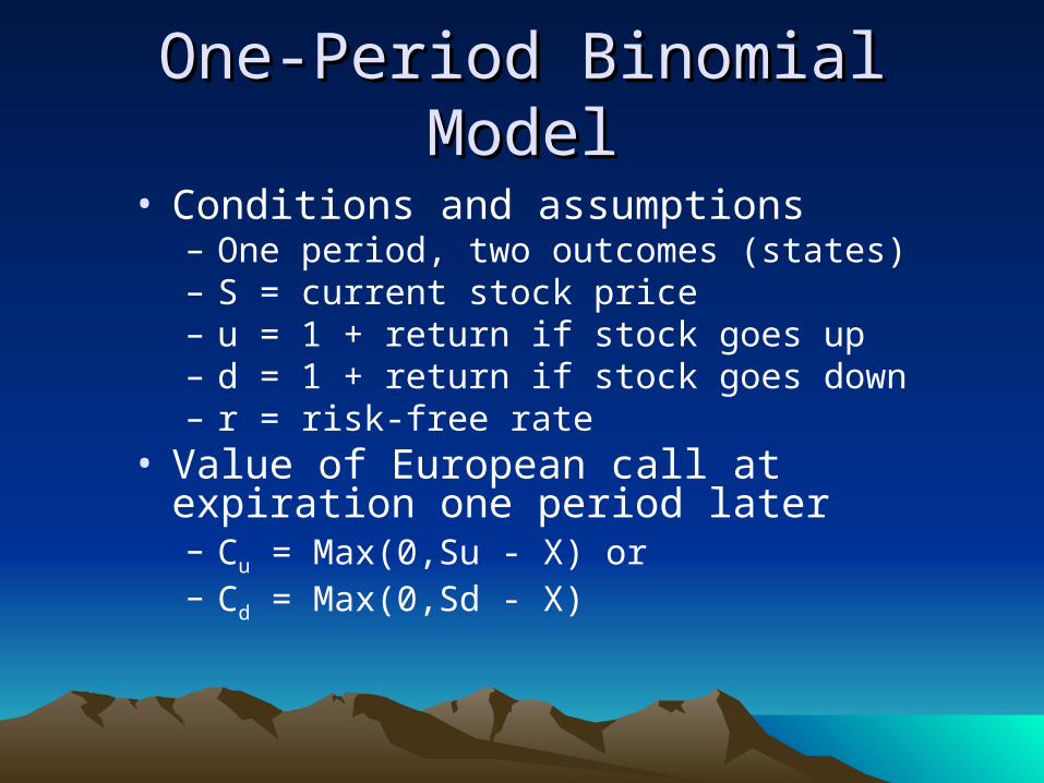
One-Period Binomial ModelOne-Period Binomial Model
• Conditions and assumptions– One period, two outcomes (states)– S = current stock price– u = 1 + return if stock goes up– d = 1 + return if stock goes down– r = risk-free rate
• Value of European call at expiration one period later– Cu = Max(0,Su - X) or– Cd = Max(0,Sd - X)
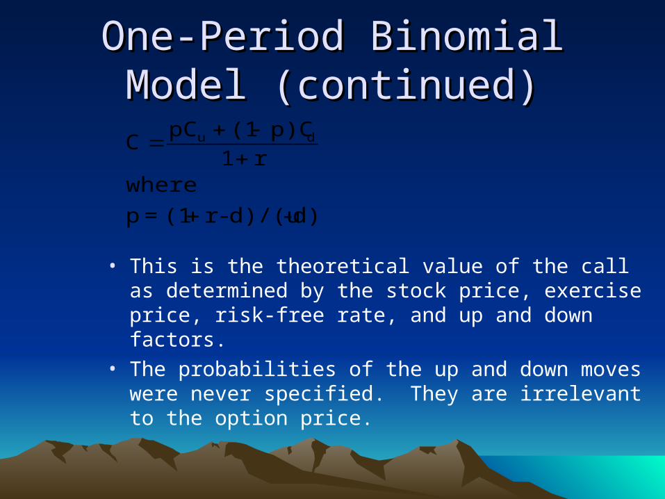
One-Period Binomial Model One-Period Binomial Model (continued)(continued)
• This is the theoretical value of the call as determined by the stock price, exercise price, risk-free rate, and up and down factors.
• The probabilities of the up and down moves were never specified. They are irrelevant to the option price.
d)-d)/(u-r(1=p
wherer1
p)C(1pCC du
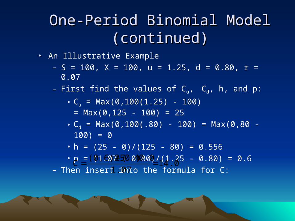
One-Period Binomial Model One-Period Binomial Model (continued)(continued)
• An Illustrative Example– S = 100, X = 100, u = 1.25, d = 0.80, r = 0.07
– First find the values of Cu, Cd, h, and p:
• Cu = Max(0,100(1.25) - 100) = Max(0,125 - 100) = 25
• Cd = Max(0,100(.80) - 100) = Max(0,80 - 100) = 0
• h = (25 - 0)/(125 - 80) = 0.556• p = (1.07 - 0.80)/(1.25 - 0.80) = 0.6
– Then insert into the formula for C: 14.02
1.07
0.0).40((0.6)25C
(Return to text slide)
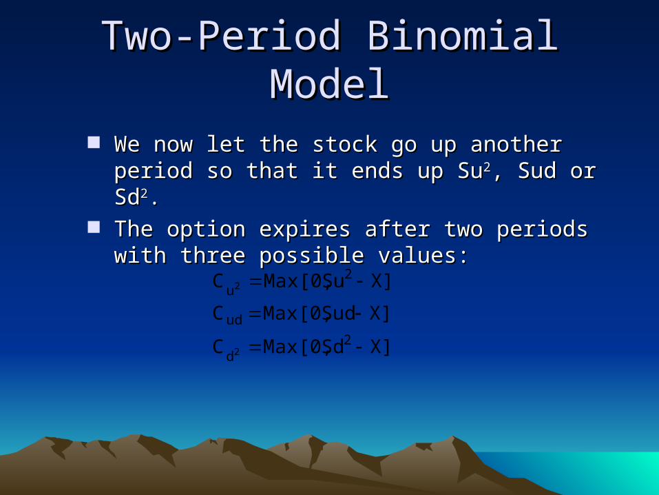
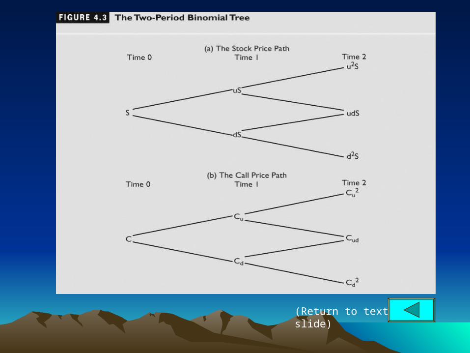
Two-Period Binomial ModelTwo-Period Binomial Model
We now let the stock go up another period so that it ends We now let the stock go up another period so that it ends up Suup Su22, Sud or Sd, Sud or Sd22..
The option expires after two periods with three possible The option expires after two periods with three possible values:values:
X]SdMax[0,C
X]SudMax[0,C
X]SuMax[0,C
2d
ud
2u
2
2
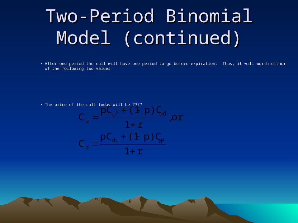
• After one period the call will have one period to go before expiration. Thus, it will worth either of the following two values
• The price of the call today will be ????
Two-Period Binomial Model Two-Period Binomial Model (continued)(continued)
r1
p)C(1pCC
or ,r1
p)C(1pCC
2
2
ddud
uduu
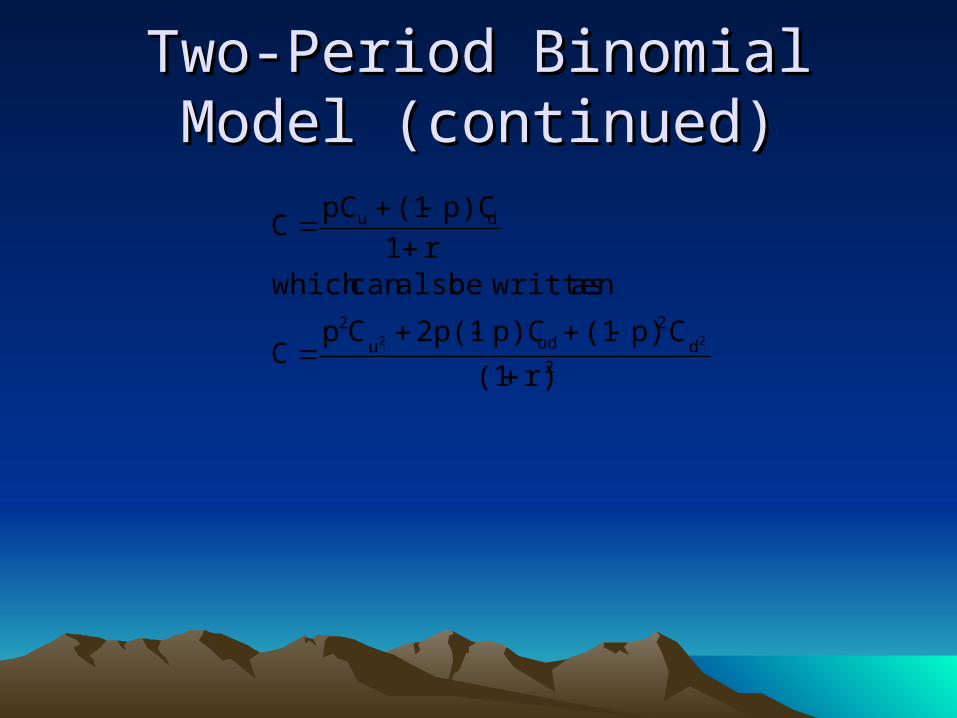
Two-Period Binomial Model Two-Period Binomial Model (continued)(continued)
2d
2udu
2
du
r)(1
Cp)(1p)C2p(1CpC
as written be alsocan which r1
p)C(1pCC
22
Two-Period Binomial Model Two-Period Binomial Model (continued)(continued)
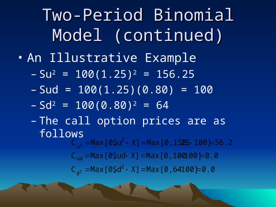
• An Illustrative Example– Su2 = 100(1.25)2 = 156.25– Sud = 100(1.25)(0.80) = 100– Sd2 = 100(0.80)2 = 64– The call option prices are as follows
0.0100]Max[0,64X]SdMax[0,C
0.0100]Max[0,100X]SudMax[0,C
56.25100]25Max[0,156.X]SuMax[0,C
2d
ud
2u
2
2
Two-Period Binomial Model Two-Period Binomial Model (continued)(continued)
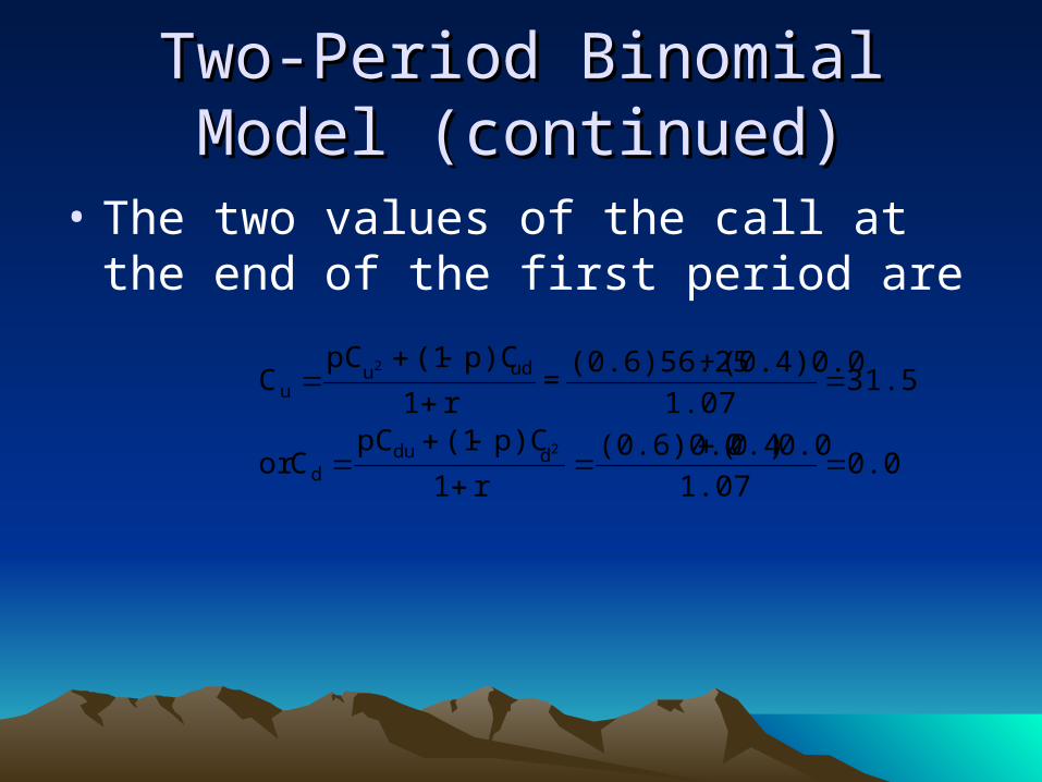
• The two values of the call at the end of the first period are
0.01.07
0.0).40((0.6)0.0
r1
p)C(1pCCor
31.541.07
(0.4)0.0+(0.6)56.25=
r1
p)C(1pCC
2
2
ddud
uduu
Two-Period Binomial Model Two-Period Binomial Model (continued)(continued)
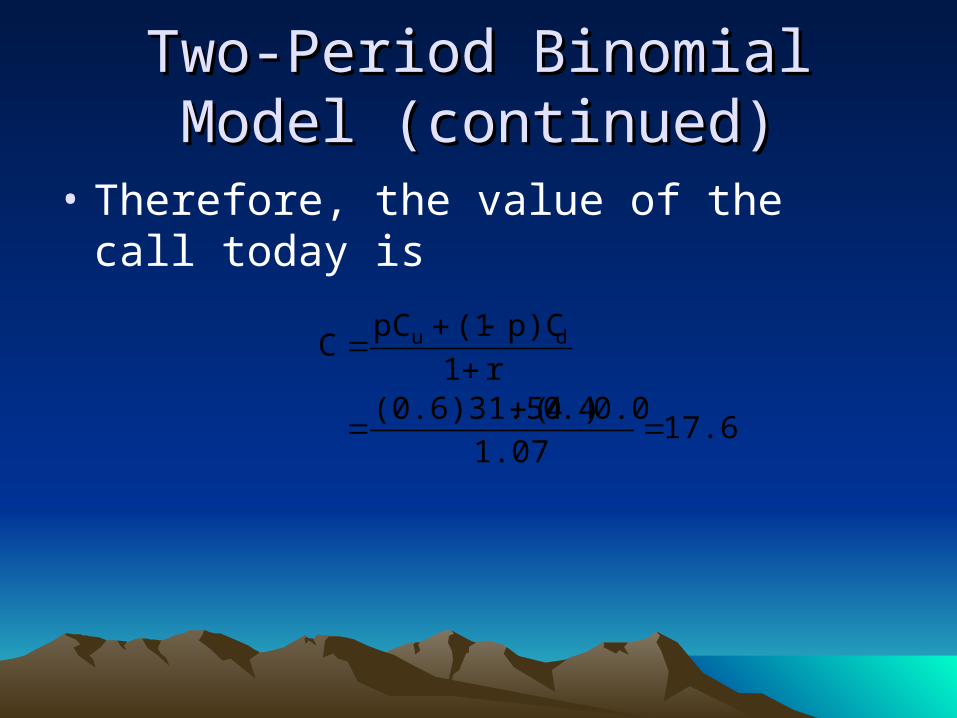
• Therefore, the value of the call today is
17.691.07
0.0).40((0.6)31.54r1
p)C(1pCC du
Next classes (4/23 & 4/28)Next classes (4/23 & 4/28)
• The concept of a hedged portfolio using options and the underlying asset (no-arbitrage model).– Show using both one and two-period binomial
models.
• Extensions of the two-period binomial model.– Put options– Binomial models and early exercise (difference
between American and European values)– An application: real options