Embed Size (px)
Citation preview
Overview of the Geometries of Shape Spaces andDiffeomorphism Groups
Martin Bauer · Martins Bruveris · Peter W. Michor
October 31, 2013
Abstract This article provides an overview of various
notions of shape spaces, including the space of parame-
trized and unparametrized curves, the space of immer-
sions, the diffeomorphism group and the space of Rie-
mannian metrics. We discuss the Riemannian metrics
that can be defined thereon, and what is known about
the properties of these metrics. We put particular em-
phasis on the induced geodesic distance, the geodesic
equation and its well-posedness, geodesic and metric
completeness and properties of the curvature.
Keywords Shape Space · Diffeomorphism Group ·Manifolds of mappings · Landmark space · Surface
matching · Riemannian geometry
Mathematics Subject Classification (2000)
58B20 · 58D15 · 35Q31
Contents
1 Introduction . . . . . . . . . . . . . . . . . . . . . . . 12 Preliminaries . . . . . . . . . . . . . . . . . . . . . . . 43 The spaces of interest . . . . . . . . . . . . . . . . . . 64 The L2-metric on plane curves . . . . . . . . . . . . . 85 Almost local metrics on shape space . . . . . . . . . 106 Sobolev type metrics on shape space . . . . . . . . . 147 Diffeomorphism groups . . . . . . . . . . . . . . . . . 188 Metrics on shape space induced by Diff(Rd) . . . . . 24
M. Bauer was supported by FWF Project P24625
Martin Bauer · Peter W. MichorFakultat fur Mathematik, Universitat Wien,Oskar-Morgenstern-Platz 1, A-1090 Wien, AustriaE-mail: [email protected]: [email protected]
Martins BruverisInstitut de mathematiques, EPFL, CH-1015,Lausanne, SwitzerlandE-mail: [email protected]
9 The space of landmarks . . . . . . . . . . . . . . . . . 2810 Universal Teichmuller space as shape space . . . . . 3011 The space of Riemannian metrics . . . . . . . . . . . 31
1 Introduction
The variability of a certain class of shapes is of in-
terest in various fields of applied mathematics and it
is of particular importance in the field of computa-
tional anatomy. In mathematics and computer vision,
shapes have been represented in many different ways:
point clouds, surfaces or images are only some exam-
ples. These shape spaces are inherently non-linear. As
an example, consider the shape space of all surfaces of
a certain dimension and genus. The nonlinearity makes
it difficult to do statistics. One way to overcome this
difficulty is to introduce a Riemannian structure on the
space of shapes. This enables us to locally linearize the
space and develop statistics based on geodesic methods.
Another advantage of the Riemannian setting for shape
analysis is its intuitive notion of similarity. Namely, two
shapes that differ only by a small deformation are re-
garded as similar to each other.
In this article we will concentrate on shape spaces
of surfaces and we will give an overview of the different
Riemannian structures, that have been considered on
these spaces.
1.1 Spaces of interest
We fix a compact manifold M without boundary of di-
mension d − 1. In this paper a shape is a submanifold
of Rd that is diffeomorphic to M and we denote by
Bi(M,Rd) and Be(M,Rd) the spaces of all immersed
and embedded submanifolds.
2 Martin Bauer et al.
Diff(M)r-acts //
r-acts
''r-acts
Imm(M,Rd)
needs gww Diff(M) (( ((
Diffc(Rd)
r-acts
l-acts
(LDDMM)
oo
l-acts
(LDDMM)xxVol+(M)
Diff(M)
Met(M)vol
oo
Diff(M)
'' ''
Bi(M,Rd)
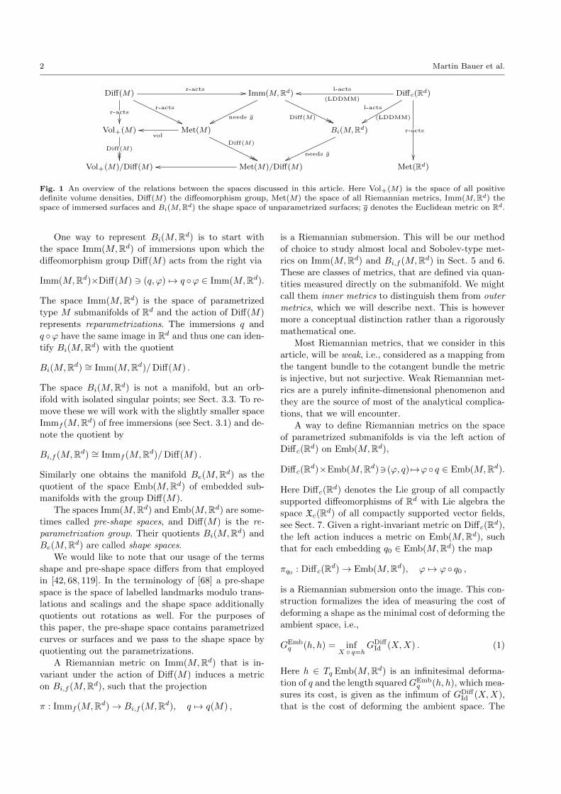
needs gwwVol+(M)/Diff(M) Met(M)/Diff(M)oo Met(Rd)
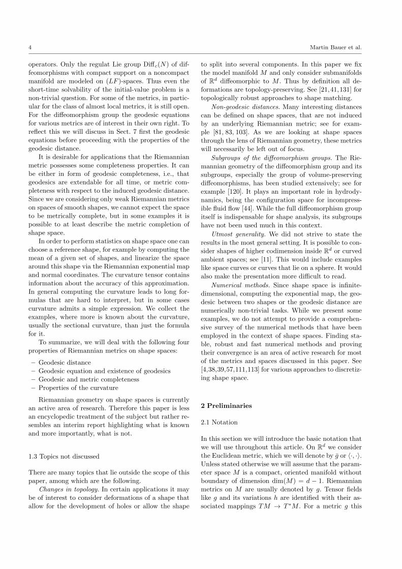
Fig. 1 An overview of the relations between the spaces discussed in this article. Here Vol+(M) is the space of all positivedefinite volume densities, Diff(M) the diffeomorphism group, Met(M) the space of all Riemannian metrics, Imm(M,Rd) thespace of immersed surfaces and Bi(M,Rd) the shape space of unparametrized surfaces; g denotes the Euclidean metric on Rd.
One way to represent Bi(M,Rd) is to start with
the space Imm(M,Rd) of immersions upon which the
diffeomorphism group Diff(M) acts from the right via
Imm(M,Rd)×Diff(M) 3 (q, ϕ) 7→ q ϕ ∈ Imm(M,Rd).
The space Imm(M,Rd) is the space of parametrized
type M submanifolds of Rd and the action of Diff(M)
represents reparametrizations. The immersions q and
q ϕ have the same image in Rd and thus one can iden-
tify Bi(M,Rd) with the quotient
Bi(M,Rd) ∼= Imm(M,Rd)/Diff(M) .
The space Bi(M,Rd) is not a manifold, but an orb-
ifold with isolated singular points; see Sect. 3.3. To re-
move these we will work with the slightly smaller space
Immf (M,Rd) of free immersions (see Sect. 3.1) and de-
note the quotient by
Bi,f (M,Rd) ∼= Immf (M,Rd)/Diff(M) .
Similarly one obtains the manifold Be(M,Rd) as the
quotient of the space Emb(M,Rd) of embedded sub-
manifolds with the group Diff(M).
The spaces Imm(M,Rd) and Emb(M,Rd) are some-
times called pre-shape spaces, and Diff(M) is the re-
parametrization group. Their quotients Bi(M,Rd) and
Be(M,Rd) are called shape spaces.
We would like to note that our usage of the terms
shape and pre-shape space differs from that employed
in [42, 68, 119]. In the terminology of [68] a pre-shape
space is the space of labelled landmarks modulo trans-
lations and scalings and the shape space additionally
quotients out rotations as well. For the purposes of
this paper, the pre-shape space contains parametrized
curves or surfaces and we pass to the shape space by
quotienting out the parametrizations.
A Riemannian metric on Imm(M,Rd) that is in-
variant under the action of Diff(M) induces a metric
on Bi,f (M,Rd), such that the projection
π : Immf (M,Rd)→ Bi,f (M,Rd), q 7→ q(M) ,
is a Riemannian submersion. This will be our method
of choice to study almost local and Sobolev-type met-
rics on Imm(M,Rd) and Bi,f (M,Rd) in Sect. 5 and 6.
These are classes of metrics, that are defined via quan-
tities measured directly on the submanifold. We might
call them inner metrics to distinguish them from outer
metrics, which we will describe next. This is however
more a conceptual distinction rather than a rigorously
mathematical one.
Most Riemannian metrics, that we consider in this
article, will be weak, i.e., considered as a mapping from
the tangent bundle to the cotangent bundle the metric
is injective, but not surjective. Weak Riemannian met-
rics are a purely infinite-dimensional phenomenon and
they are the source of most of the analytical complica-
tions, that we will encounter.
A way to define Riemannian metrics on the space
of parametrized submanifolds is via the left action of
Diffc(Rd) on Emb(M,Rd),
Diffc(Rd)×Emb(M,Rd)3(ϕ, q) 7→ϕ q ∈ Emb(M,Rd).
Here Diffc(Rd) denotes the Lie group of all compactly
supported diffeomorphisms of Rd with Lie algebra the
space Xc(Rd) of all compactly supported vector fields,
see Sect. 7. Given a right-invariant metric on Diffc(Rd),the left action induces a metric on Emb(M,Rd), such
that for each embedding q0 ∈ Emb(M,Rd) the map
πq0 : Diffc(Rd)→ Emb(M,Rd), ϕ 7→ ϕ q0 ,
is a Riemannian submersion onto the image. This con-
struction formalizes the idea of measuring the cost of
deforming a shape as the minimal cost of deforming the
ambient space, i.e.,
GEmbq (h, h) = inf
X q=hGDiff
Id (X,X) . (1)
Here h ∈ Tq Emb(M,Rd) is an infinitesimal deforma-
tion of q and the length squaredGEmbq (h, h), which mea-
sures its cost, is given as the infimum of GDiffId (X,X),
that is the cost of deforming the ambient space. The
Overview of Shape Spaces 3
infimum is taken over all X ∈ Xc(Rd) infinitesimal de-
formations of Rd, that equal h when restricted to q.
This motivates the name outer metrics, since they are
defined in terms of deformations of the ambient space.
The natural space to define these metrics is the
space of embeddings instead of immersions, because not
all orbits of the Diffc(Rd) action on Imm(M,Rd) are
open. Defining a Riemannian metric on Be(M,Rd) is
now a two step process
Diffc(Rd)πq0 //Emb(M,Rd) π //Be(M,Rd) .
One starts with a right-invariant Riemannian metric
on Diffc(Rd), which descends via (1) to a metric on
Emb(M,Rd). This metric is invariant under the repa-
rametrization group and thus descends to a metric on
Be(M,Rd). These metrics are studied in Sect. 8.
Riemannian metrics on the diffeomorphism groups
Diffc(Rd) and Diff(M) are of interest, not only because
these groups act as the deformation group of the ambi-
ent space and the reparametrization group respectively.
They are related to the configuration spaces for hydro-
dynamics and various PDEs arising in physics can be in-
terpreted as geodesic equations on the diffeomorphism
group. While a geodesic on Diffc(Rd) is a curve ϕ(t) of
diffeomorphisms, its right-logarithmic derivative u(t) =
∂tϕ(t) ϕ(t)−1 is a curve of vector fields. If the metric
on Diffc(Rd) is given as GId(u, v) =∫Rd〈Lu, v〉dx with
a differential operator L, then the geodesic equation can
be written in terms of u(t) as
∂tm+ (u · ∇)m+m div u+DuT .m = 0, m = Lu .
PDEs that are special cases of this equation include the
Camassa-Holm equation, the Hunter-Saxton equationand others. See Sect. 7 for details.
So far we encoded shape through the way it lies in
the ambient space; i.e., either as a map q : M → Rd or
as its image q(M). One can also look at how the map q
deforms the model space M . Denote by g the Euclidean
metric on Rd and consider the pull-back map
Imm(M,Rd)→ Met(M), q 7→ q∗g , (2)
where Met(M) is the space of all Riemannian metrics
on M and q∗g denotes the pull-back of g to a metric on
M . Depending on the dimension of M one can expect
to capture more or less information about shape with
this map. Elements of Met(M) with dim(M) = d − 1
are symmetric, positive definite tensor fields of type(
02
)and thus have d(d−1)
2 components. Immersions on the
other hand are maps from M into Rd and thus have
d components. For d = 3, the case of surfaces in R3,
the number of components coincide, while for d > 3 we
have d(d−1)2 > d. Thus we would expect the pull-back
map to capture most aspects of shape. The pull-back is
equivariant with respect to Diff(M) and thus we have
the commutative diagram
Immf (M,Rd)q 7→q∗g //
Met(M)
Bi,f (M,Rd) // Met(M)/Diff(M)
The space in the lower right corner is not far away from
Met(M)/Diff0(M), where Diff0(M) denotes the con-
nected component of the identity. This space, known as
super space, is used in general relativity. Little is known
about the properties of the pull-back map (2), but as a
first step it is of interest to consider Riemannian met-
rics on the space Met(M). This is done in Sect. 11, with
special emphasis on the L2- or Ebin-metric.
1.2 Questions discussed
After having explained the spaces, that will play the
main roles in the paper and the relationships between
them, what are the questions that we will be asking?
The questions are motivated by applications to com-
paring shapes.
After equipping the space with a Riemannian met-
ric, the simplest way to compare shapes is by looking
at the matrix of pairwise distances, measured with the
induced geodesic distance function. Thus an important
question is, whether the geodesic distance function is
point-separating, that is whether for two distinct shapes
C0 6= C1 we have d(C0, C1) > 0. In finite dimensions
the answer to this question is always “yes”. Even more,
a standard result of Riemannian geometry states that
the topology induced by the geodesic distance coin-
cides with the manifold topology. In infinite dimensions,
when the manifold is equipped with a weak Rieman-
nian metric, this is in general not true any more. The
topology induced by the geodesic distance will also be
weaker than the manifold topology. We will therefore
survey what is known about the geodesic distance and
the topology it induces.
The path realizing the distance between two shapes
is, if it exists, a geodesic. So it is natural to look at
the geodesic equation on the manifold. In finite dimen-
sions the geodesic equation is an ODE, the initial value
problem for geodesics can be solved, at least for short
times, and the solution depends smoothly on the ini-
tial data. The manifolds of interest in this paper are
naturally modeled mostly as Frechet manifolds and in
coordinates the geodesic equation is usually a partial
differential equation or even involves pseudo differential
4 Martin Bauer et al.
operators. Only the regulat Lie group Diffc(N) of dif-
feomorphisms with compact support on a noncompact
manifold are modeled on (LF )-spaces. Thus even the
short-time solvability of the initial-value problem is a
non-trivial question. For some of the metrics, in partic-
ular for the class of almost local metrics, it is still open.
For the diffeomorphism group the geodesic equations
for various metrics are of interest in their own right. To
reflect this we will discuss in Sect. 7 first the geodesic
equations before proceeding with the properties of the
geodesic distance.
It is desirable for applications that the Riemannian
metric possesses some completeness properties. It can
be either in form of geodesic completeness, i.e., that
geodesics are extendable for all time, or metric com-
pleteness with respect to the induced geodesic distance.
Since we are considering only weak Riemannian metrics
on spaces of smooth shapes, we cannot expect the space
to be metrically complete, but in some examples it is
possible to at least describe the metric completion of
shape space.
In order to perform statistics on shape space one can
choose a reference shape, for example by computing the
mean of a given set of shapes, and linearize the space
around this shape via the Riemannian exponential map
and normal coordinates. The curvature tensor contains
information about the accuracy of this approximation.
In general computing the curvature leads to long for-
mulas that are hard to interpret, but in some cases
curvature admits a simple expression. We collect the
examples, where more is known about the curvature,
usually the sectional curvature, than just the formula
for it.
To summarize, we will deal with the following four
properties of Riemannian metrics on shape spaces:
– Geodesic distance
– Geodesic equation and existence of geodesics
– Geodesic and metric completeness
– Properties of the curvature
Riemannian geometry on shape spaces is currently
an active area of research. Therefore this paper is less
an encyclopedic treatment of the subject but rather re-
sembles an interim report highlighting what is known
and more importantly, what is not.
1.3 Topics not discussed
There are many topics that lie outside the scope of this
paper, among which are the following.
Changes in topology. In certain applications it may
be of interest to consider deformations of a shape that
allow for the development of holes or allow the shape
to split into several components. In this paper we fix
the model manifold M and only consider submanifolds
of Rd diffeomorphic to M . Thus by definition all de-
formations are topology-preserving. See [21,41,131] for
topologically robust approaches to shape matching.
Non-geodesic distances. Many interesting distances
can be defined on shape spaces, that are not induced
by an underlying Riemannian metric; see for exam-
ple [81, 83, 103]. As we are looking at shape spaces
through the lens of Riemannian geometry, these metrics
will necessarily be left out of focus.
Subgroups of the diffeomorphism groups. The Rie-
mannian geometry of the diffeomorphism group and its
subgroups, especially the group of volume-preserving
diffeomorphisms, has been studied extensively; see for
example [120]. It plays an important role in hydrody-
namics, being the configuration space for incompress-
ible fluid flow [44]. While the full diffeomorphism group
itself is indispensable for shape analysis, its subgroups
have not been used much in this context.
Utmost generality. We did not strive to state the
results in the most general setting. It is possible to con-
sider shapes of higher codimension inside Rd or curved
ambient spaces; see [11]. This would include examples
like space curves or curves that lie on a sphere. It would
also make the presentation more difficult to read.
Numerical methods. Since shape space is infinite-
dimensional, computing the exponential map, the geo-
desic between two shapes or the geodesic distance are
numerically non-trivial tasks. While we present some
examples, we do not attempt to provide a comprehen-
sive survey of the numerical methods that have been
employed in the context of shape spaces. Finding sta-
ble, robust and fast numerical methods and proving
their convergence is an area of active research for most
of the metrics and spaces discussed in this paper. See
[4,38,39,57,111,113] for various approaches to discretiz-
ing shape space.
2 Preliminaries
2.1 Notation
In this section we will introduce the basic notation that
we will use throughout this article. On Rd we consider
the Euclidean metric, which we will denote by g or 〈·, ·〉.Unless stated otherwise we will assume that the param-
eter space M is a compact, oriented manifold without
boundary of dimension dim(M) = d − 1. Riemannian
metrics on M are usually denoted by g. Tensor fields
like g and its variations h are identified with their as-
sociated mappings TM → T ∗M . For a metric g this
Overview of Shape Spaces 5
yields the musical isomorphisms
[ : TM → T ∗M and ] : T ∗M → TM.
Immersions from M to Rd – i.e., smooth mappings with
everywhere injective derivatives – are denoted by q and
the corresponding unit normal field of an (orientable)
immersion q is denoted by nq. For every immersion q :
M → Rd we consider the induced pull-back metric g =
q∗g on M given by
q∗g(X,Y ) = g(Tq.X, Tq.Y ),
for vector fields X,Y ∈ X(M). Here Tq denotes the
tangent mapping of the map q : M → Rd. We will
denote the induced volume form of the metric g = q∗g
as vol(g). In positively oriented coordinates (u, U) it is
given by
vol(g) =√
det(g (∂iq, ∂jq)) du1 ∧ · · · ∧ dud−1 .
Using the volume form we can calculate the total vol-
ume Volq =∫M
vol(q∗g) of the immersion q.
The Levi-Civita covariant derivative determined by
a metric g will be denoted by ∇g and we will consider
the induced Bochner–Laplacian ∆g, which is defined for
all vector fields X ∈ X(M) via
∆gX = −Tr(g−1∇2X) .
Note that in Rd the usual Laplacian ∆ is the negative
of the Bochner–Laplacian of the Euclidean metric, i.e.,
∆g = −∆.
Furthermore, we will need the second fundamental
form sq(X,Y ) = g(∇q∗gX Tq.Y, nq
). Using it we can
define the Gauß curvature Kq = det(g−1sq) and the
mean curvature Hq = Tr(g−1sq).
In the special case of plane curves (M = S1 and
d = 2) we use the letter c for the immersed curve. The
curve parameter θ ∈ S1 will be the positively oriented
parameter on S1, and differentiation ∂θ will be denoted
by the subscript θ, i.e., cθ = ∂θc. We will use a similar
notation for the time derivative of a time dependent
family of curves, i.e., ∂tc = ct.
We denote the corresponding unit length tangent
vector by
v = vc =cθ|cθ|
= −Jnc where J =√−1 on C = R2 ,
and nc is the unit length tangent vector. The covariant
derivative of the pull-back metric reduces to arclength
derivative, and the induced volume form to arclength
integration:
Ds =∂θ|cθ|
, ds = |cθ|dθ.
Using this notation the length of a curve can be written
as
`c =
∫S1
ds .
In this case Gauß and mean curvature are the same and
are denoted by κ = 〈Dsv, n〉.
2.2 Riemannian submersions
In this article we will repeatedly induce a Riemannian
metric on a quotient space using a given metric on the
top space. The concept of a Riemannian submersion will
allow us to achieve this goal in an elegant manner. We
will now explain in general terms what a Riemannian
submersion is and how geodesics in the quotient space
correspond to horizontal geodesics in the top space.
Let (E,GE) be a possibly infinite dimensional weak
Riemannian manifold; weak means that GE : TE →T ∗E is injective, but need not be surjective. A conse-
quence is that the Levi-Civita connection (equivalently,
the geodesic equation) need not exist; however, if the
Levi-Civita connection does exist, it is unique. Let Gbe a smooth possibly infinite dimensional regular Lie
group; see [77] or [76, Section 38] for the notion used
here, or [106] for a more general notion of Lie group. Let
G×E → E be a smooth group action on E and assume
that B := E/G is a manifold. Denote by π : E → B the
projection, which is then a submersion of smooth man-
ifolds by which we means that it admits local smooth
sections everywhere; in particular, Tπ : TE → TB is
surjective. Then
Ver = Ver(π) := ker(Tπ) ⊂ TE
is called the vertical subbundle. Assume that GE is in
addition invariant under the action of G. Then the ex-
pression
‖Y ‖2GB := inf‖X‖2GE : X ∈ TxE, Tπ.X = Y
defines a semi-norm on B. If it is a norm, it can be
shown (by polarization pushed through the completion)
that this norm comes from a weak Riemannian metric
GB on B; then the projection π : E → B is a Rieman-
nian submersion.
Sometimes the the GE-orthogonal space Ver(π)⊥ ⊂TE is a fiber-linear complement in TE. In general, the
orthogonal space is a complement (for the GE-closure
of Ver(π)) only if taken in the fiberwise GE-completionTE of TE. This leads to the notion of a robust Rieman-
nian manifold: a Riemannian manifold (E,GE) is called
robust, if TE is a smooth vector-bundle over E and
the Levi-Civita connection of GE exists and is smooth.
6 Martin Bauer et al.
See [88] for details. We will encounter examples, where
the use of TE is necessary in Sect. 8.
The horizontal subbundle Hor = Hor(π,G) is the
GE-orthogonal complement of Ver in TE or in TE,
respectively. Any vector X ∈ TE can be decomposed
uniquely in vertical and horizontal components as
X = Xver +Xhor .
Note that if we took the complement in TE, i.e., Hor ⊂TE, then in general Xver ∈ Ver. The mapping
Txπ|Horx : Horx → Tπ(x)B or Tπ(x)B
is a linear isometry of (pre-)Hilbert spaces for all x ∈ E.
Here Tπ(x)B is the fiber-wise GB-completion of Tπ(x)B.
We are not claiming that TB forms a smooth vector-
bundle over B although this will be true in the examples
considered in Sect. 8.
Theorem 2.1 Consider a Riemannian submersion π :
E → B between robust weak Riemannian manifolds,
and let γ : [0, 1]→ E be a geodesic in E.
1. If γ′(t) is horizontal at one t, then it is horizontal
at all t.
2. If γ′(t) is horizontal then π γ is a geodesic in B.
3. If every curve in B can be lifted to a horizontal curve
in E, then, up to the choice of an initial point, there
is a one-to-one correspondence between curves in B
and horizontal curves in E. This implies that in-
stead of solving the geodesic equation in B one can
equivalently solve the equation for horizontal geode-
sics in E.
See [92, Sect. 26] for a proof, and [88] for the case of
robust Riemannian manifolds.
3 The spaces of interest
3.1 Immersions and embeddings
Parametrized surfaces will be modeled as immersions
or embeddings of the configuration manifold M into
Rd. We call immersions and embeddings parametrized
since a change in their parametrization (i.e., applying a
diffeomorphism on the domain of the function) results
in a different object. We will deal with the following
sets of functions:
Emb(M,Rd) ⊂ Immf (M,Rd)⊂ Imm(M,Rd) ⊂ C∞(M,Rd) .
(3)
Here C∞(M,Rd) is the set of smooth functions from M
to Rd, Imm(M,Rd) is the set of all immersions of M
into Rd, i.e., all functions q ∈ C∞(M,Rd) such that Txq
is injective for all x ∈M . The set Immf (M,Rd) consists
of all free immersions q; i.e., the diffeomorphism group
of M acts freely on q, i.e., q ϕ = q implies ϕ = IdMfor all ϕ ∈ Diff(M).
By [26, Lem. 3.1], the isotropy group Diff(M)q :=
ϕ ∈ Diff(M) : q ϕ = q of any immersion q is al-
ways a finite group which acts properly discontinuously
on M so that M → M/Diff(M)q is a covering map.
Emb(M,N) is the set of all embeddings of M into Rd,i.e., all immersions q that are homeomorphisms onto
their image.
Theorem 3.1 The spaces Imm(M,Rd), Immf (M,Rd)and Emb(M,Rd) are Frechet manifolds.
Proof Since M is compact by assumption it follows that
C∞(M,Rd) is a Frechet manifold by [76, Sect. 42.3];
see also [58], [90]. All inclusions in (3) are inclusions of
open subsets: first Imm(M,Rd) is open in C∞(M,Rd)since the condition that the differential is injective at
every point is an open condition on the one-jet of q [90,
Sect. 5.1]. Immf (M,Rd) is open in Imm(M,Rd) by [26,
Thm. 1.5]. Emb(M,Rd) is open in Immf (M,Rd) by [76,
Thm. 44.1]. Thus all the spaces are Frechet manifolds
as well.
3.2 Shape space
Unparametrized surfaces are equivalence classes of pa-
rametrized surfaces under the action of the reparame-
trization group.
Theorem 3.2 (Thm. 1.5, [26]) The quotient space
Bi,f (M,Rd) := Immf (M,Rd)/Diff(M)
is a smooth Hausdorff manifold and the projection
π : Immf (M,Rd)→ Bi,f (M,Rd)
is a smooth principal fibration with Diff(M) as structure
group.
For q ∈ Immf (M,Rd) we can define a chart around
π(q) ∈ Bi,f (M,Rd) by
π ψq : C∞(M, (−ε, ε))→ Bi,f (M,Rd)
with ε sufficiently small, where
ψq : C∞(M, (−ε, ε))→ Immf (M,Rd)
is defined by ψq(a) = q + anq and nq is the unit-length
normal vector to q.
Corollary 3.3 The statement of Thm. 3.2 does not
change, if we replace Bi,f (M,Rd) by Be(M,Rd) and
Immf (M,Rd) by Emb(M,Rd).
Overview of Shape Spaces 7
The result for embeddings is proven in [18,58,89,90].
As Emb(M,Rd) is an open subset of Immf (M,Rd) and
is Diff(M)-invariant, the quotient
Be(M,Rd) := Emb(M,Rd)/Diff(M)
is an open subset of Bi,f (M,Rd) and as such itself a
smooth principal bundle with structure group Diff(M).
3.3 Some words on orbifolds
The projection
Imm(M,Rd)→ Bi(M,Rd) := Imm(M,Rd)/Diff(M)
is the prototype of a Riemannian submersion onto an
infinite dimensional Riemannian orbifold. In the arti-
cle [122, Prop. 2.1] it is stated that the finite dimen-
sional Riemannian orbifolds are exactly of the form
M/G for a Riemannian manifold M and a compact
group G of isometries with finite isotropy groups. Cur-
vature on Riemannian orbifolds is well defined, and it
suffices to treat it on the dense regular subset. In our
case Bi,f (M,Rd) is the regular stratum of the orbifold
Bi(M,Rd). For the behavior of geodesics on Rieman-
nian orbit spaces M/G see for example [1]; the easiest
way to carry these results over to infinite dimensions
is by using Gauss’ lemma, which only holds if the Rie-
mannian exponential mapping is a diffeomorphism on
an GImm-open neighborhood of 0 in each tangent space.
This is rarely true.
Given a Diff(M)-invariant Riemannian metric on
Imm(M,Rd), one can define a metric distance distBi on
Bi(M,Rd) by taking as distance between two shapes
the infimum of the lengths of all (equivalently, hor-
izontal) smooth curves connecting the corresponding
Diff(M)-orbits. There are the following questions:
– Does distBi separate points? In many cases this has
been decided.
– Is (Bi(M,Rd),distBi) a geodesic metric space? In
other words, does there exists a rectifiable curve
connecting two shapes in the same connected com-
ponent whose length is exactly the distance? This is
widely open, but it is settled as soon as local mini-
mality of geodesics in Imm(M,Rd) is established.
In this article we are discussing Riemannian met-
rics on Bi,f (M,Rd), that are induced by Riemannian
metrics on Immf (M,Rd) via Riemannian submersions.
However all metrics on Immf (M,Rd), that we consider,
arise as restrictions of metrics on Imm(M,R2). Thus,
when dealing with parametrized shapes, we will use the
space Imm(M,R2) and restrict ourselves to the open
and dense subset Immf (M,R2), whenever we consider
the space Bi,f (M,R2) of unparametrized shapes.
3.4 Diffeomorphism group
Concerning the Lie group structure of the diffeomor-
phism group we have the following theorem.
Theorem 3.4 (Thm. 43.1, [76]) Let M be a smooth
manifold, not necessarily compact. The group
Diffc(M) =ϕ : ϕ,ϕ−1 ∈ C∞(M,M),
x : ϕ(x) 6= x has compact closure
of all compactly supported diffeomorphisms is an open
submanifold of C∞(M,M) (equipped wit a refinement
of the Whitney C∞-topology) and composition and in-
version are smooth maps. It is a regular Lie group and
the Lie algebra is the space Xc(M) of all compactly sup-
ported vector fields, whose bracket is the negative of the
usual Lie bracket.
An infinite dimensional smooth Lie group G with
Lie algebra g is called regular, if the following two con-
ditions hold:
– For each smooth curve X ∈ C∞(R, g) there exists
a unique smooth curve g ∈ C∞(R, G) whose right
logarithmic derivative is X, i.e.,
g(0) = e
∂tg(t) = Te(µg(t))X(t) = X(t).g(t) .
(4)
Here µg : G→ G denotes the right multiplication:
µgx = x.g .
– The map evolrG : C∞(R, g) → G is smooth, where
evolrG(X) = g(1) and g is the unique solution of (4).
IfM is compact, then all diffeomorphisms have com-
pact support and Diffc(M) = Diff(M). For Rn the
group Diff(Rd) of all orientation preserving diffeomor-
phisms is not an open subset of C∞(Rd,Rd) endowed
with the compact C∞-topology and thus it is not a
smooth manifold with charts in the usual sense. There-
fore, it is necessary to work with the smaller space
Diffc(Rd) of compactly supported diffeomorphisms. In
Sect. 7 we will also introduce the groups DiffH∞(Rd)and DiffS(Rd) with weaker decay conditions towards
infinity. Like Diffc(Rd) they are smooth regular Lie
groups.
3.5 The space of Riemannian metrics
We denote by Met(M) the space of all smooth Rieman-
nian metrics. Each g ∈ Met(M) is a symmetric, positive
definite(
02
)tensor field on M , or equivalently a point-
wise positive definite section of the bundle S2T ∗M .
8 Martin Bauer et al.
Theorem 3.5 (Sect. 1.1, [52]) Let M be a compact
manifold without boundary. The space Met(M) of all
Riemannian metrics on M is an open subset of the
space Γ (S2T ∗M) of all symmetric(
02
)tensor fields and
thus itself a smooth Frechet-manifold.
For each g ∈ Met(M) and x ∈ M we can regard
g(x) as either a map
g(x) : TxM × TxM → R
or as an invertible map
gx : TxM → T ∗xM .
The latter interpretation allows us to compose g, h ∈Met(M) to obtain a fiber-linear map g−1.h : TM →TM .
4 The L2-metric on plane curves
4.1 Properties of the L2-metric
We first look at the simplest shape space, the space of
plane curves. In order to induce a metric on the mani-
fold of un-parametrized curves Bi,f (S1,R2) we need to
define a metric on parametrized curves Imm(S1,R2),
that is invariant under reparametrizations, c.f. Sect. 2.2.
The simplest such metric on the space of immersed
plane curves is the L2-type metric
G0c(h, k) =
∫S1
〈h(θ), k(θ)〉ds .
The horizontal bundle of this metric, when restricted
to Immf (S1,R2), consists of all tangent vectors, h thatare pointwise orthogonal to cθ, i.e., h(θ) = a(θ)nc(θ)
for some scalar function a ∈ C∞(S1). An expression
for the metric on the quotient space Bi,f (S1,R2), using
the charts from Thm. 3.2, is given by
G0C(Tcπ(a.nc), Tcπ(b.nc)) =
∫S1
a(θ)b(θ) ds .
This metric was first studied in the context of shape
analysis in [95]. The geodesic equation for theG0-metric
on Immf (S1,R2) is given by
(|cθ|ct)t = −1
2
(|ct|2cθ|cθ|
)θ
. (5)
Geodesics on Bi,f (S1,R2) correspond to horizontal geo-
desics on Immf (S1,R2) by Thm. 2.1; these satisfy ct =
a.nc, with a scalar function a(t, θ). Thus the geodesic
equation (5) reduces to an equation for a(t, θ),
at =1
2κa2 .
Note that this is not an ODE for a, because κc, being
the curvature of c, depends implicitly on a. It is however
possible to eliminate κ and arrive at (see [95, Sect. 4.3])
att − 4a2t
a− a6aθθ
2w4+a6aθwθw5
− a5a2θ
w4= 0
w(θ) = a(0, θ)√|cθ(0, θ)| ,
a nonlinear hyperbolic PDE of second order.
Open question. Are the geodesic equations on either
of the spaces Imm(S1,R2) or Bi,f (S1,R2) for the L2-
metric (locally) well-posed?
The L2-metric is among the few for which the sec-
tional curvature on Bi,f (S1,R2) has a simple expres-
sion. Let C = π(c) ∈ Bi,f (S1,R2) and choose c ∈Immf (S1,R2) such that it is parametrized by constant
speed. Take a.nc, b.nc ∈ HorG0(c) two orthonormal hor-
izontal tangent vectors at c. Then the sectional cur-
vature of the plane spanned by them is given by the
Wronskian
kC(P (Tcπ(a.nc), Tcπ(b.nc)) =1
2
∫S1
(abθ − aθb)2ds .
(6)
In particular the sectional curvature is non-negative
and unbounded.
Remark 4.1 This metric has a natural generalization
to the space Imm(M,Rd) of immersions of an arbitrary
compact manifold M . This can be done by replacing
the integration over arc-length with integration over the
volume form of the induced pull-back metric. For q ∈Imm(M,Rd) the metric is defined by
G0q(h, k) =
∫M
〈h(x), k(x)〉 vol(q∗g) .
The geodesic spray of this metric was computed in [17]
and the curvature in [65].
For all its simplicity the main drawback of the L2-
metric is that the induced geodesic distance vanishes
on Imm(S1,R2). If c : [0, 1] → Imm(S1,R2) is a path,
denote by
LenGImm(c) =
∫ 1
0
√Gc(t)(ct(t), ct(t)) dt
its length. The geodesic distance between two points is
defined as the infimum of the pathlength over all paths
connecting the two points,
distGImm(c0, c1) = infc(0)=c0,c(1)=c1
LenGImm(c) .
Overview of Shape Spaces 9
For a finite dimensional Riemannian manifold (M,G)
this distance is always positive, due to the local inverti-
bility of the exponential map. This does not need to be
true for a weak Riemannian metric in infinite dimen-
sions and the L2-metric on Bi,f (S1,R2) was the first
known example, where this was indeed false. We have
the following result.
Theorem 4.2 The geodesic distance function induced
by the metric G0 vanishes identically on Imm(S1,R2)
and Bi,f (S1,R2).
For any two curves c0, c1 ∈ Imm(S1,R2) and ε > 0
there exists a smooth path c : [0, 1]→ Imm(S1,R2) with
c(0) = c0, c(1) = c1 and length LenG0
Imm(c) < ε.
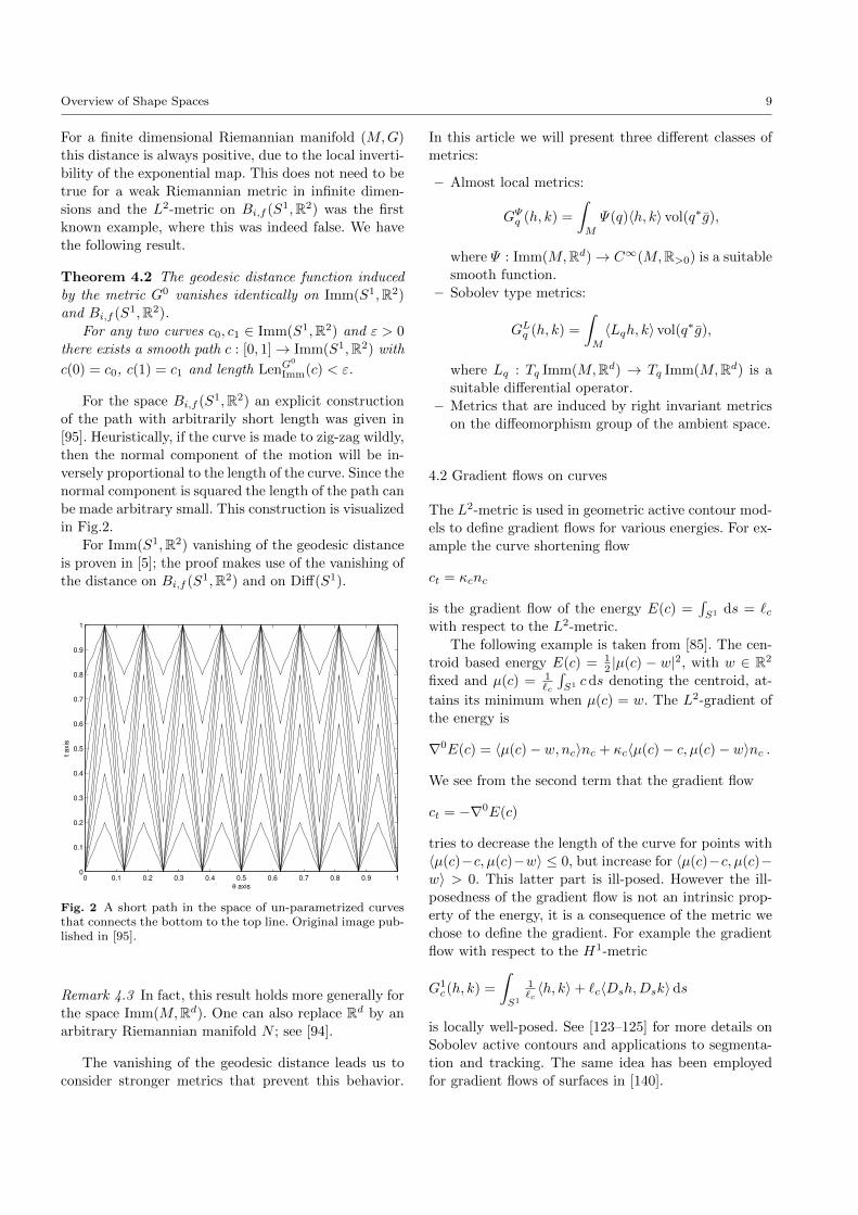
For the space Bi,f (S1,R2) an explicit construction
of the path with arbitrarily short length was given in
[95]. Heuristically, if the curve is made to zig-zag wildly,
then the normal component of the motion will be in-
versely proportional to the length of the curve. Since the
normal component is squared the length of the path can
be made arbitrary small. This construction is visualized
in Fig.2.
For Imm(S1,R2) vanishing of the geodesic distance
is proven in [5]; the proof makes use of the vanishing of
the distance on Bi,f (S1,R2) and on Diff(S1).
0 0.1 0.2 0.3 0.4 0.5 0.6 0.7 0.8 0.9 10
0.1
0.2
0.3
0.4
0.5
0.6
0.7
0.8
0.9
1
θ axis
t axis
Fig. 2 A short path in the space of un-parametrized curvesthat connects the bottom to the top line. Original image pub-lished in [95].
Remark 4.3 In fact, this result holds more generally for
the space Imm(M,Rd). One can also replace Rd by an
arbitrary Riemannian manifold N ; see [94].
The vanishing of the geodesic distance leads us to
consider stronger metrics that prevent this behavior.
In this article we will present three different classes of
metrics:
– Almost local metrics:
GΨq (h, k) =
∫M
Ψ(q)〈h, k〉 vol(q∗g),
where Ψ : Imm(M,Rd)→ C∞(M,R>0) is a suitable
smooth function.
– Sobolev type metrics:
GLq (h, k) =
∫M
〈Lqh, k〉 vol(q∗g),
where Lq : Tq Imm(M,Rd) → Tq Imm(M,Rd) is a
suitable differential operator.
– Metrics that are induced by right invariant metrics
on the diffeomorphism group of the ambient space.
4.2 Gradient flows on curves
The L2-metric is used in geometric active contour mod-
els to define gradient flows for various energies. For ex-
ample the curve shortening flow
ct = κcnc
is the gradient flow of the energy E(c) =∫S1 ds = `c
with respect to the L2-metric.
The following example is taken from [85]. The cen-
troid based energy E(c) = 12 |µ(c) − w|2, with w ∈ R2
fixed and µ(c) = 1`c
∫S1 cds denoting the centroid, at-
tains its minimum when µ(c) = w. The L2-gradient of
the energy is
∇0E(c) = 〈µ(c)− w, nc〉nc + κc〈µ(c)− c, µ(c)− w〉nc .
We see from the second term that the gradient flow
ct = −∇0E(c)
tries to decrease the length of the curve for points with
〈µ(c)−c, µ(c)−w〉 ≤ 0, but increase for 〈µ(c)−c, µ(c)−w〉 > 0. This latter part is ill-posed. However the ill-
posedness of the gradient flow is not an intrinsic prop-
erty of the energy, it is a consequence of the metric we
chose to define the gradient. For example the gradient
flow with respect to the H1-metric
G1c(h, k) =
∫S1
1`c〈h, k〉+ `c〈Dsh,Dsk〉ds
is locally well-posed. See [123–125] for more details on
Sobolev active contours and applications to segmenta-
tion and tracking. The same idea has been employed
for gradient flows of surfaces in [140].
10 Martin Bauer et al.
5 Almost local metrics on shape space
Almost local metrics are metrics of the form
GΨq (h, k) =
∫M
Ψ(q)〈h, k〉 vol(q∗g) ,
where Ψ : Imm(M,Rd) → C∞(M,R>0) is a smooth
function that is equivariant with respect to the action
of Diff(M), i.e.,
Ψ(q ϕ) = Ψ(q) ϕ , q ∈ Imm(M,Rd) , ϕ ∈ Diff(M) .
Equivariance of Ψ then implies the invariance of GΨ and
thus GΨ induces a Riemannian metric on the quotient
Bi,f (M,Rd).Examples of almost local metrics that have been
considered are of the form
GΦq (h, k) =
∫M
Φ(Volq, Hq,Kq)〈h, k〉 vol(q∗g) , (7)
where Φ ∈ C∞(R3,R>0) is a function of the total vol-
ume Volq, the mean curvature Hq and the Gauß cur-
vature Kq. The name “almost local” is derived from
the fact that while Hq and Kq are local quantities, the
total volume Volq induces a mild non-locality in the
metric. If Φ = Φ(Vol) depends only on the total vol-
ume, the resulting metric is conformally equivalent to
the L2-metric, the latter corresponding to Φ ≡ 1.
For an almost local metric GΨ the horizontal bundle
at q ∈ Immf (M,Rd) consists of those tangent vectors
h that are pointwise orthogonal to q,
HorΨ (q) = h ∈ Tq Immf (M,Rd) :
h = a.nq , a ∈ C∞(M,R) .
Using the charts from Thm. 3.2, the metric GΨ on
Bi,f (M,Rd) is given by
GΨπ(q) (Tqπ(a.nq), Tqπ(b.nq)) =
∫M
Ψ(q).a.b vol(q∗g) ,
with a, b ∈ C∞(M,R).
Almost local metrics, that were studied in more de-
tail include the curvature weighted GA-metrics
GAc (h, k) =
∫S1
(1 +Aκ2c)〈h, k〉ds , (8)
with A > 0 in [95] and the conformal rescalings of the
L2-metric
GΦc (h, k) = Φ(`c)
∫S1
〈h, k〉ds ,
with Φ ∈ C∞(R>0,R>0) in [115,135], both on the space
of plane curves. More general almost local metrics on
the space of plane curves were considered in [96] and
they have been generalized to hypersurfaces in higher
dimensions in [3, 12,13].
5.1 Geodesic distance
Under certain conditions on the function Ψ almost local
metrics are strong enough to induce a point-separating
geodesic distance function on the shape space.
Theorem 5.1 If Ψ satisfies one of the following con-
ditions
1. Ψ(q) ≥ 1 +AH2q
2. Ψ(q) ≥ AVolq
for some A > 0, then the metric GΨ induces a point-
separating geodesic distance function on Bi,f (M,Rd),i.e., for C0 6= C1 we have distΨBi,f (C0, C1) > 0.
For planar curves the result under assumption 1 is
proven in [95, Sect. 3.4] and under assumption 2 in [115,
Thm. 3.1]. The proof was generalized to the space of
hypersurfaces in higher dimensions in [12, Thm. 8.7].
The proof is based on the observation that under
the above assumptions the GΨ -length of a path of im-
mersions can be bounded from below by the area swept
out by the path. A second ingredient in the proof is the
Lipschitz-continuity of the function√
Volq.
Theorem 5.2 If Ψ satisfies
Ψ(q) ≥ 1 +AH2q ,
then the geodesic distance satisfies∣∣∣√VolQ1−√
VolQ2
∣∣∣ ≤ 1
2√A
distGΨ
Bi,f(Q1, Q2) .
In particular the map
√Vol : (Bi,f (M,Rd),distG
Ψ
Bi,f)→ R≥0
is Lipschitz continuous.
This result is proven in [95, Sect. 3.3] for plane
curves and in [12, Lem. 8.4] for hypersurfaces in higher
dimensions.
In the case of planar curves [115] showed that for
the almost local metric with Ψ(c) = `c the geodesic
distance on Bi,f (S1,R2) is not only bounded by but
equal to the infimum over the area swept out,
dist`Bi,f (C0, C1) = infπ(c(0))=C0
π(c(1))=C1
∫S1×[0,1]
|det dc(t, θ)| dθ dt.
Remark 5.3 No almost local metric can induce a point
separating geodesic distance function on Immf (M,Rd)and thus neither on Imm(M,Rd). When we restrict
the metric GΨ to an orbit q Diff(M) of the Diff(M)-
action, the induced metric on the space q Diff(M) ∼=
Overview of Shape Spaces 11
Diff(M) is a right-invariant weighted L2-type metric,
for which the geodesic distance vanishes. Thus
distΨImm(q, q ϕ) = 0 ,
for all q ∈ Immf (M,Rd) and ϕ ∈ Diff(M). See Sect.
7.4 for further details.
This is not a contradiction to Thm. 5.1, since a
point-separating distance on the quotient Bi,f (M,Rd)only implies that the distance on Immf (M,Rd) sepa-
rates the fibers of the projection π : Bi,f (M,Rd) →Immf (M,Rd). On each fiber π−1(C) ⊂ Immf (M,Rd)the distance can still be vanishing, as it is the case for
the almost local metrics.
It is possible to compare the geodesic distance on
shape space with the Frechet distance. The Frechet dis-
tance is defined as
distL∞
Bi,f(Q0, Q1) = inf
q0,q1‖q0 − q1‖L∞ , (9)
where the infimum is taken over all immersions q0, q1
with π(qi) = Qi. Depending on the behavior of the
metric under scaling, it may or may not be possible to
bound the Frechet distance by the geodesic distance.
Theorem 5.4 (Thm. 8.9, [12]) If Ψ satisfies one of
the conditions,
1. Ψ(q) ≤ C1 + C2H2kq
2. Ψ(q) ≤ C1 Volkq ,
with some constants C1, C2 > 0 and k < d+12 , then
there exists no constant C > 0, such that
distL∞
Bi,f(Q0, Q1) ≤ C distΨBi,f (Q0, Q1) ,
holds for all Q0, Q1 ∈ Bi,f (M,Rd).
Note that this theorem also applies to theGA-metric
for planar curves defined in (8). Even though Thm. 5.4
states that the identity map
ι :(Bi,f (S1,R2),distG
A)→(Bi,f (S1,R2),distL
∞)
is not Lipschitz continuous, it can be shown that is
continuous and thus the topology induces by distGA
is
stronger than that induced by distL∞
.
Theorem 5.5 (Cor. 3.6, [95]) The identity map on
Bi,f (S1,R2) is continuous from (Bi,f (S1,R2),distGA
)
to (Bi,f (S1,R2),distL∞
) and uniformly continuous on
every subset, where the length `C is bounded.
As a corollary to this result we obtain another proof
that the geodesic distance for the GA-metric is point-
separating on Bi,f (S1,R2).
5.2 Geodesic equation
Since geodesics on Bi,f correspond to horizontal geo-
desics on Immf (M,Rd), see Thm. 2.1, to compute the
geodesic equation on Bi,f (M,Rd) it is enough to re-
strict the geodesic equation on Immf (M,Rd) to hori-
zontal curves.
As an example for the resulting equations we will
present the geodesic equations on Bi,f (M,Rd) for the
almost local metric with Ψ(q) = 1 + AH2q , which is a
generalization of the metric (8), and the family of met-
rics with Ψ(q) = Φ(Volq), which are conformal rescal-
ings of the L2-metric.
Theorem 5.6 Geodesics of the almost local GΨ -metric
with Ψ(q) = 1 + AH2q on Bi,f (M,Rd) are given by so-
lutions of
qt = anq , g = q∗g ,
at = 12a
2Hq + 2A1+AH2
qg(Hq∇ga+ 2a∇gHq,∇ga)
− Aa2
1+AH2q
(∆gHq + Tr
((g−1sq
)2)).
For the family of metrics with Ψ(q) = Φ(Volq) geodesics
are given by
qt =b(t)
Φ(Volq)nq , g = q∗g ,
at =Hq
2Φ(Volq)
(a2 − Φ′(Volq)
Φ(Volq)
∫M
a2 vol(g)
).
For the GA-metric and planar curves the geodesic equa-
tion was calculated in [95, Sect. 4.1], whereas for con-
formal metrics on planar curves it is presented in [115,
Sect. 4]. For hypersurfaces in higher dimensions the
equations are calculated in [12, Sect. 10.2 and 10.3].
Note that both for A = 0 and Φ(q) ≡ 1 one recovers
the geodesic equation for the L2-metric,
at =1
2Hqa
2.
Similarly to the case of the L2-metric it is unknown,
whether the geodesic equations are well-posed.
Open question. Are the geodesic equations on either
of the spaces Imm(M,R2) or Bi,f (M,R2) for the almost
local metrics (locally) well-posed?
5.3 Conserved quantities
If the map Ψ is equivariant with respect to the Diff(M)-
action, then the GΨ -metric is invariant, and we obtain
12 Martin Bauer et al.
by Noether’s theorem that the reparametrization mo-
mentum is constant along each geodesic. The repara-
metrization momentum for the GΨ -metric is given by
Ψ(q)g(q>t , ·) vol(q∗g) ∈ Γ (T ∗M ⊗ Λd−1T ∗M) ,
with g = q∗g and the pointwise decomposition of the
tangent vector qt = q>t + q⊥t of qt into q⊥t = g(qt, nq)nqand q>t (x) ∈ Tq(x)q(M). This means that for each X ∈X(M) we have∫M
Ψ(q)g(q>t , X) vol(q∗g) = const.
If Ψ is additionally invariant under the action of
the Euclidean motion group Rd o SO(d), i.e., Ψ(O.q +
v) = Ψ(q), then so is the GΨ -metric and by Noether’s
theorem the linear and angular momenta are constant
along geodesics. These are given by∫M
Ψ(q)qt vol(q∗g) ∈ Rd∫M
Ψ(q) q ∧ qt vol(q∗g) ∈∧2
Rd ∼= so(d)∗ .
The latter means that for each Ω ∈ so(d) the quantity∫M
Ψ(q)g(Ω.q, qt) vol(q∗g)
is constant along geodesics.
If the function Ψ satisfies the scaling property
Ψ(λq) = λ− dim(M)−2Ψ(q), q ∈ Imm(M,Rd), λ ∈ R>0,
then the induced metric GΨ is scale invariant. In this
case the scaling momenta are conserved along geodesics
as well:∫M
Ψ(q)〈q, qt〉 vol(q∗g) scaling momentum
For plane curves the momenta are∫S1
Ψ(c)〈cθ, ct〉µds reparametrization momentum∫S1
Ψ(c)ct ds linear momentum∫S1
〈Jc, ct〉ds angular momentum∫S1
Ψ(c)〈c, ct〉ds scaling momentum
with µ ∈ C∞(S1) and J denoting rotation by π2 .
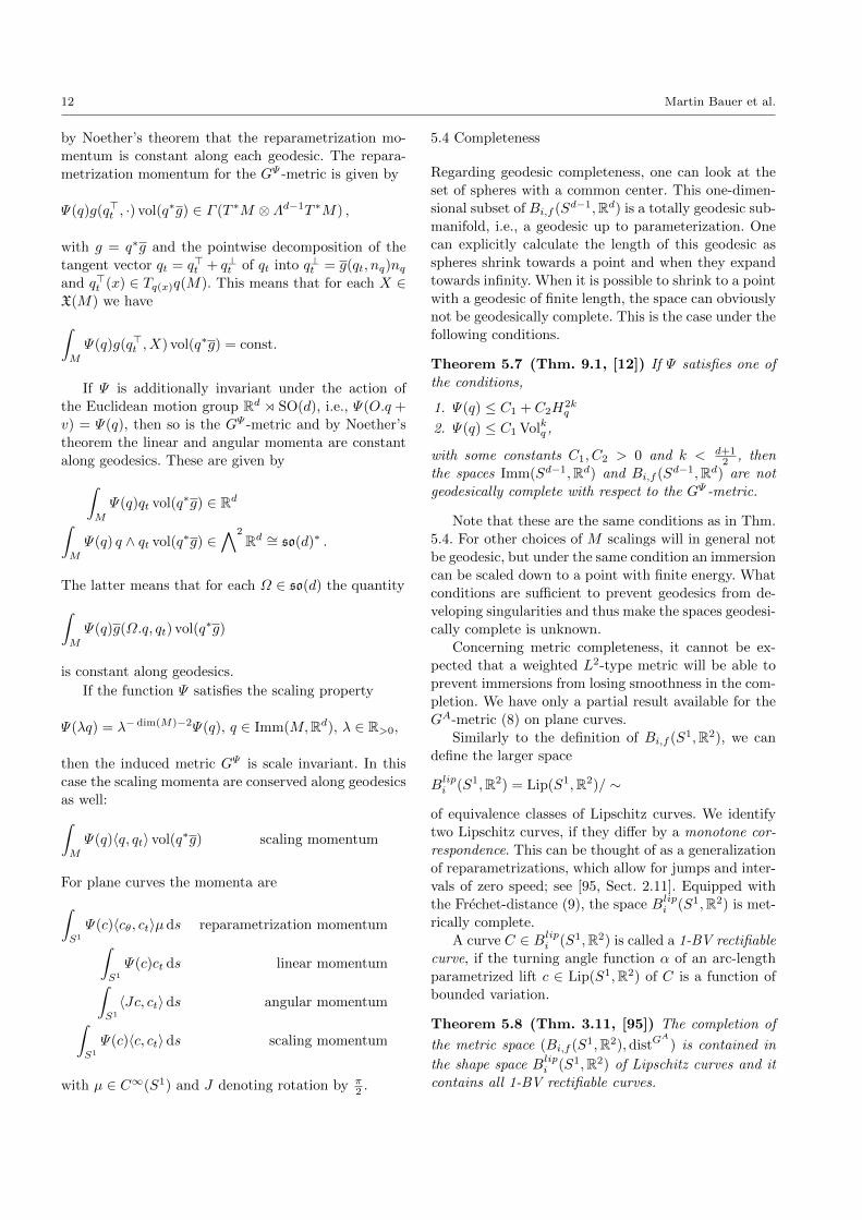
5.4 Completeness
Regarding geodesic completeness, one can look at the
set of spheres with a common center. This one-dimen-
sional subset of Bi,f (Sd−1,Rd) is a totally geodesic sub-
manifold, i.e., a geodesic up to parameterization. One
can explicitly calculate the length of this geodesic as
spheres shrink towards a point and when they expand
towards infinity. When it is possible to shrink to a point
with a geodesic of finite length, the space can obviously
not be geodesically complete. This is the case under the
following conditions.
Theorem 5.7 (Thm. 9.1, [12]) If Ψ satisfies one of
the conditions,
1. Ψ(q) ≤ C1 + C2H2kq
2. Ψ(q) ≤ C1 Volkq ,
with some constants C1, C2 > 0 and k < d+12 , then
the spaces Imm(Sd−1,Rd) and Bi,f (Sd−1,Rd) are not
geodesically complete with respect to the GΨ -metric.
Note that these are the same conditions as in Thm.
5.4. For other choices of M scalings will in general not
be geodesic, but under the same condition an immersion
can be scaled down to a point with finite energy. What
conditions are sufficient to prevent geodesics from de-
veloping singularities and thus make the spaces geodesi-
cally complete is unknown.
Concerning metric completeness, it cannot be ex-
pected that a weighted L2-type metric will be able to
prevent immersions from losing smoothness in the com-
pletion. We have only a partial result available for the
GA-metric (8) on plane curves.
Similarly to the definition of Bi,f (S1,R2), we can
define the larger space
Blipi (S1,R2) = Lip(S1,R2)/ ∼
of equivalence classes of Lipschitz curves. We identify
two Lipschitz curves, if they differ by a monotone cor-
respondence. This can be thought of as a generalization
of reparametrizations, which allow for jumps and inter-
vals of zero speed; see [95, Sect. 2.11]. Equipped with
the Frechet-distance (9), the space Blipi (S1,R2) is met-
rically complete.
A curve C ∈ Blipi (S1,R2) is called a 1-BV rectifiable
curve, if the turning angle function α of an arc-length
parametrized lift c ∈ Lip(S1,R2) of C is a function of
bounded variation.
Theorem 5.8 (Thm. 3.11, [95]) The completion of
the metric space (Bi,f (S1,R2),distGA
) is contained in
the shape space Blipi (S1,R2) of Lipschitz curves and it
contains all 1-BV rectifiable curves.
Overview of Shape Spaces 13
5.5 Curvature
The main challenge in computing the curvature for al-
most local metrics on Imm(M,Rd) is finding enough
paper to finish the calculations. It is probably due to
this that apart from the L2-metric we are not aware of
any curvature calculations on the space Imm(M,Rd).For the quotient space Bi,f (M,Rd) the situation is a
bit better and the formulas a bit shorter. This is be-
cause Bi,f (M,Rd) is modeled on C∞(M,R), while the
space Imm(M,Rd) is modeled on C∞(M,Rd). In co-
ordinates elements of Bi,f (M,Rd) are represented by
scalar functions, while immersions need functions with
d components. For plane curves and conformal met-
rics the curvature has been calculated in [115] and for
Ψ(c) = Φ(`c, κc) in [96]. Similarly for higher dimen-
sional surfaces the curvature has been calculated for
Ψ(q) = Φ(Volq, Hq) in [12].
The sectional curvature for the L2-metric on plane
curves (6) is non-negative. In general the expression for
the sectional curvature for almost local metrics with
Φ 6≡ 1 will contain both positive definite, negative def-
inite and indefinite terms. For example the sectional
curvature of the metric (8) with Ψ(c) = 1 + Aκ2c on
plane curves has the following form.
Theorem 5.9 (Sect. 4.6, [95]) Let C ∈ Bi,f (S1,R2)
and choose c ∈ Imm(S1,R2) such that C = π(c) and c
is parametrized by constant speed. Let a.n, b.n ∈ Hor(c)
two orthonormal horizontal tangent vectors at c. Then
the sectional curvature of the plane spanned by a, b ∈TCBi,f (S1,R2) for the GA metric is
kC(P (a, b)) = −∫S1
A(a.D2sb− b.D2
sa)2ds
+
∫(1−Aκ2)2 − 4A2κ.D2
sκ+ 8A2(Dsκ)2
2(1 +Aκ2)·
· (a.Dsb − b.Dsa)2ds
It is assumed, although not proven at the moment,
that for a generic immersion, similar to Thm. 7.14, the
sectional curvature will assume both signs.
5.6 Examples
To conclude the section we want to present some ex-
amples of numerical solutions to the geodesic boundary
value problem for given shapes Q0, Q1 ∈ Bi,f (M,Rd)with metrics of the form (7). One method to tackle this
problem is to directly minimize the horizontal path en-
ergy
Ehor(q) =
∫ 1
0
∫M
Φ(Volq, Hq)〈qt, nq〉2 vol(q∗g) dt
over the set of paths q of immersions with fixed end-
points q0, q1 that project onto the target surfaces Q0
and Q1, i.e., π(qi) = Qi. The main advantage of this
approach for the class of almost local metrics lies in
the simple form of the horizontal bundle. Although we
will only show one specific example in this article it is
worth to note that several numerical experiments are
available; see:
– [95, 96] for the GA–metric and planar curves.
– [135,136] for conformal metrics and planar curves.
– [3, 12,13] for surfaces in R3.
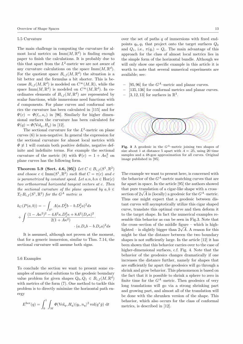
Fig. 3 A geodesic in the GA–metric joining two shapes ofsize about 1 at distance 5 apart with A = .25, using 20 timesamples and a 48-gon approximation for all curves. Originalimage published in [95].
The example we want to present here, is concerned with
the behavior of the GA-metric matching curves that are
far apart in space. In the article [95] the authors showed
that pure translation of a cigar-like shape with a cross–
section of 2√A is (locally) a geodesic for theGA–metric.
Thus one might expect that a geodesic between dis-
tant curves will asymptotically utilize this cigar shaped
curve, translate this optimal curve and then deform it
to the target shape. In fact the numerical examples re-
semble this behavior as can be seen in Fig.3. Note that
the cross–section of the middle figure – which is high-
lighted – is slightly bigger than 2√A. A reason for this
might be that the distance between the two boundary
shapes is not sufficiently large. In the article [12] it has
been shown that this behavior carries over to the case of
higher-dimensional surfaces, c.f. Fig. 4. Note that the
behavior of the geodesics changes dramatically if one
increases the distance further, namely for shapes that
are sufficiently far apart the geodesics will go through a
shrink and grow behavior. This phenomenon is based on
the fact that it is possible to shrink a sphere to zero in
finite time for the GA–metric. Then geodesics of very
long translations will go via a strong shrinking part
and growing part, and almost all of the translation will
be done with the shrunken version of the shape. This
behavior, which also occurs for the class of conformal
metrics, is described in [12].
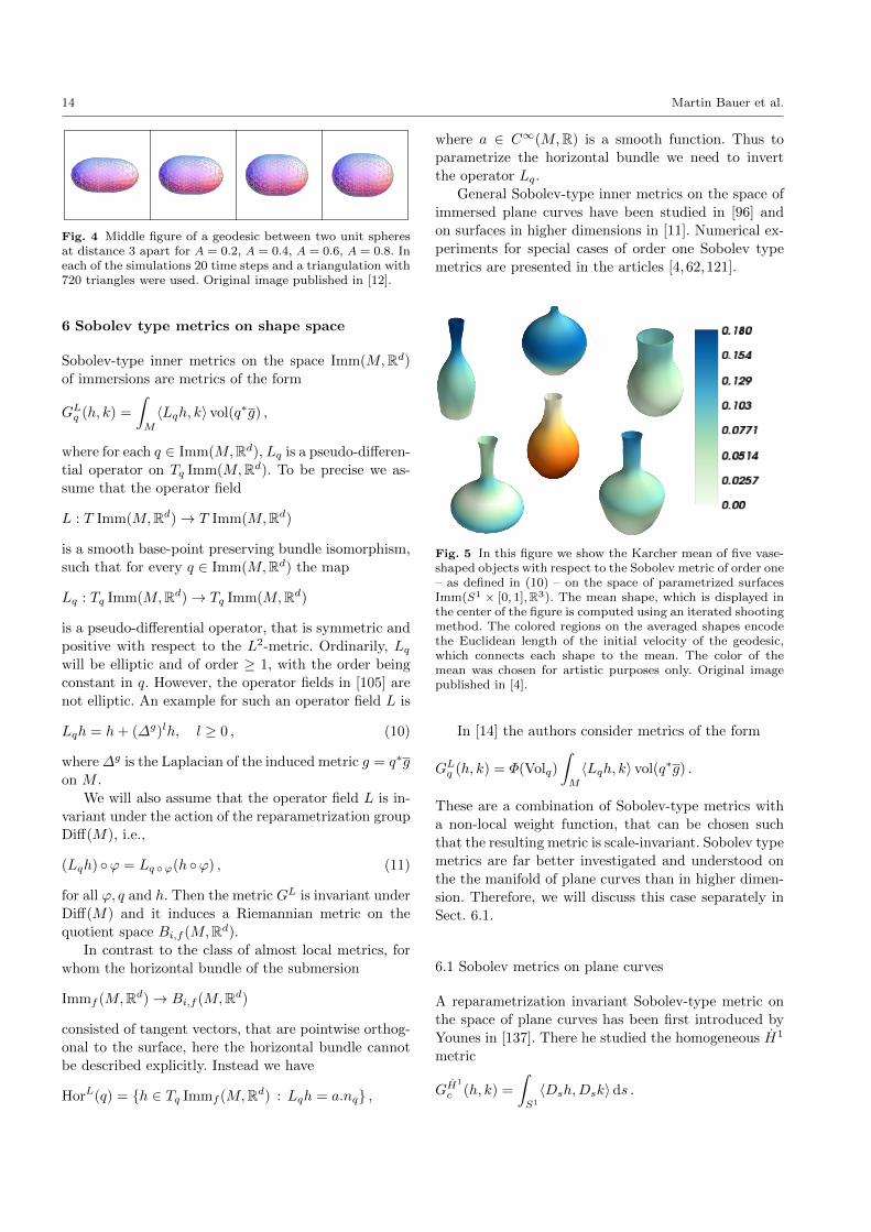
14 Martin Bauer et al.
Fig. 4 Middle figure of a geodesic between two unit spheresat distance 3 apart for A = 0.2, A = 0.4, A = 0.6, A = 0.8. Ineach of the simulations 20 time steps and a triangulation with720 triangles were used. Original image published in [12].
6 Sobolev type metrics on shape space
Sobolev-type inner metrics on the space Imm(M,Rd)of immersions are metrics of the form
GLq (h, k) =
∫M
〈Lqh, k〉 vol(q∗g) ,
where for each q ∈ Imm(M,Rd), Lq is a pseudo-differen-
tial operator on Tq Imm(M,Rd). To be precise we as-
sume that the operator field
L : T Imm(M,Rd)→ T Imm(M,Rd)
is a smooth base-point preserving bundle isomorphism,
such that for every q ∈ Imm(M,Rd) the map
Lq : Tq Imm(M,Rd)→ Tq Imm(M,Rd)
is a pseudo-differential operator, that is symmetric and
positive with respect to the L2-metric. Ordinarily, Lqwill be elliptic and of order ≥ 1, with the order being
constant in q. However, the operator fields in [105] are
not elliptic. An example for such an operator field L is
Lqh = h+ (∆g)lh, l ≥ 0 , (10)
where∆g is the Laplacian of the induced metric g = q∗g
on M .
We will also assume that the operator field L is in-
variant under the action of the reparametrization group
Diff(M), i.e.,
(Lqh) ϕ = Lq ϕ(h ϕ) , (11)
for all ϕ, q and h. Then the metric GL is invariant under
Diff(M) and it induces a Riemannian metric on the
quotient space Bi,f (M,Rd).In contrast to the class of almost local metrics, for
whom the horizontal bundle of the submersion
Immf (M,Rd)→ Bi,f (M,Rd)
consisted of tangent vectors, that are pointwise orthog-
onal to the surface, here the horizontal bundle cannot
be described explicitly. Instead we have
HorL(q) = h ∈ Tq Immf (M,Rd) : Lqh = a.nq ,
where a ∈ C∞(M,R) is a smooth function. Thus to
parametrize the horizontal bundle we need to invert
the operator Lq.
General Sobolev-type inner metrics on the space of
immersed plane curves have been studied in [96] and
on surfaces in higher dimensions in [11]. Numerical ex-
periments for special cases of order one Sobolev type
metrics are presented in the articles [4, 62,121].
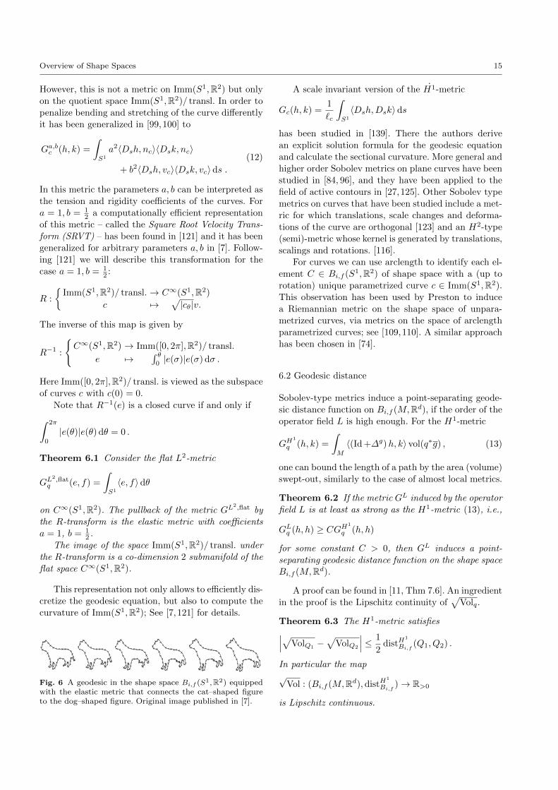
Fig. 5 In this figure we show the Karcher mean of five vase-shaped objects with respect to the Sobolev metric of order one– as defined in (10) – on the space of parametrized surfacesImm(S1 × [0, 1],R3). The mean shape, which is displayed inthe center of the figure is computed using an iterated shootingmethod. The colored regions on the averaged shapes encodethe Euclidean length of the initial velocity of the geodesic,which connects each shape to the mean. The color of themean was chosen for artistic purposes only. Original imagepublished in [4].
In [14] the authors consider metrics of the form
GLq (h, k) = Φ(Volq)
∫M
〈Lqh, k〉 vol(q∗g) .
These are a combination of Sobolev-type metrics with
a non-local weight function, that can be chosen such
that the resulting metric is scale-invariant. Sobolev type
metrics are far better investigated and understood on
the the manifold of plane curves than in higher dimen-
sion. Therefore, we will discuss this case separately in
Sect. 6.1.
6.1 Sobolev metrics on plane curves
A reparametrization invariant Sobolev-type metric on
the space of plane curves has been first introduced by
Younes in [137]. There he studied the homogeneous H1
metric
GH1
c (h, k) =
∫S1
〈Dsh,Dsk〉ds .
Overview of Shape Spaces 15
However, this is not a metric on Imm(S1,R2) but only
on the quotient space Imm(S1,R2)/ transl. In order to
penalize bending and stretching of the curve differently
it has been generalized in [99,100] to
Ga,bc (h, k) =
∫S1
a2〈Dsh, nc〉〈Dsk, nc〉
+ b2〈Dsh, vc〉〈Dsk, vc〉ds .(12)
In this metric the parameters a, b can be interpreted as
the tension and rigidity coefficients of the curves. For
a = 1, b = 12 a computationally efficient representation
of this metric – called the Square Root Velocity Trans-
form (SRVT) – has been found in [121] and it has been
generalized for arbitrary parameters a, b in [7]. Follow-
ing [121] we will describe this transformation for the
case a = 1, b = 12 :
R :
Imm(S1,R2)/ transl. → C∞(S1,R2)
c 7→√|cθ|v.
The inverse of this map is given by
R−1 :
C∞(S1,R2)→ Imm([0, 2π],R2)/ transl.
e 7→∫ θ
0|e(σ)|e(σ) dσ .
Here Imm([0, 2π],R2)/ transl. is viewed as the subspace
of curves c with c(0) = 0.
Note that R−1(e) is a closed curve if and only if∫ 2π
0
|e(θ)|e(θ) dθ = 0 .
Theorem 6.1 Consider the flat L2-metric
GL2,flat
q (e, f) =
∫S1
〈e, f〉dθ
on C∞(S1,R2). The pullback of the metric GL2,flat by
the R-transform is the elastic metric with coefficients
a = 1, b = 12 .
The image of the space Imm(S1,R2)/ transl. under
the R-transform is a co-dimension 2 submanifold of the
flat space C∞(S1,R2).
This representation not only allows to efficiently dis-
cretize the geodesic equation, but also to compute the
curvature of Imm(S1,R2); See [7, 121] for details.
Fig. 6 A geodesic in the shape space Bi,f (S1,R2) equippedwith the elastic metric that connects the cat–shaped figureto the dog–shaped figure. Original image published in [7].
A scale invariant version of the H1-metric
Gc(h, k) =1
`c
∫S1
〈Dsh,Dsk〉ds
has been studied in [139]. There the authors derive
an explicit solution formula for the geodesic equation
and calculate the sectional curvature. More general and
higher order Sobolev metrics on plane curves have been
studied in [84, 96], and they have been applied to the
field of active contours in [27,125]. Other Sobolev type
metrics on curves that have been studied include a met-
ric for which translations, scale changes and deforma-
tions of the curve are orthogonal [123] and an H2-type
(semi)-metric whose kernel is generated by translations,
scalings and rotations. [116].
For curves we can use arclength to identify each el-
ement C ∈ Bi,f (S1,R2) of shape space with a (up to
rotation) unique parametrized curve c ∈ Imm(S1,R2).
This observation has been used by Preston to induce
a Riemannian metric on the shape space of unpara-
metrized curves, via metrics on the space of arclength
parametrized curves; see [109,110]. A similar approach
has been chosen in [74].
6.2 Geodesic distance
Sobolev-type metrics induce a point-separating geode-
sic distance function on Bi,f (M,Rd), if the order of the
operator field L is high enough. For the H1-metric
GH1
q (h, k) =
∫M
〈(Id +∆g)h, k〉 vol(q∗g) , (13)
one can bound the length of a path by the area (volume)
swept-out, similarly to the case of almost local metrics.
Theorem 6.2 If the metric GL induced by the operator
field L is at least as strong as the H1-metric (13), i.e.,
GLq (h, h) ≥ CGH1
q (h, h)
for some constant C > 0, then GL induces a point-
separating geodesic distance function on the shape space
Bi,f (M,Rd).
A proof can be found in [11, Thm 7.6]. An ingredient
in the proof is the Lipschitz continuity of√
Volq.
Theorem 6.3 The H1-metric satisfies∣∣∣√VolQ1 −√
VolQ2
∣∣∣ ≤ 1
2distH
1
Bi,f(Q1, Q2) .
In particular the map√
Vol : (Bi,f (M,Rd),distH1
Bi,f)→ R>0
is Lipschitz continuous.
16 Martin Bauer et al.
A proof for plane curves can be found in [96, Sect.
4.7] and for higher dimensional surfaces in [11, Lem.
7.5].
The behavior of the geodesic distance on the space
Immf (M,Rd) is unknown. Similar to Sect. 5.1 we can
restrict the GL-metric to an orbit q Diff(M) and the
induced metric on Diff(M) will be a right-invariant
Sobolev metric. Since Sobolev-type metrics of a suffi-
ciently high order on the diffeomorphism group have
point-separating geodesic distance functions, there is
no a-priori obstacle for the distance distLImm not to be
point-separating.
Open question. Under what conditions on the opera-
tor field L does the metric GL induce a point-separating
geodesic distance function on Immf (M,Rd)?
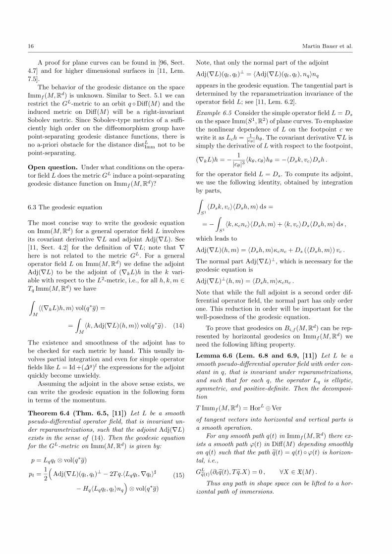
6.3 The geodesic equation
The most concise way to write the geodesic equation
on Imm(M,Rd) for a general operator field L involves
its covariant derivative ∇L and adjoint Adj(∇L). See
[11, Sect. 4.2] for the definition of ∇L; note that ∇here is not related to the metric GL. For a general
operator field L on Imm(M,Rd) we define the adjoint
Adj(∇L) to be the adjoint of (∇kL)h in the k vari-
able with respect to the L2-metric, i.e., for all h, k,m ∈Tq Imm(M,Rd) we have∫M
〈(∇kL)h,m〉 vol(q∗g) =
=
∫M
〈k,Adj(∇L)(h,m)〉 vol(q∗g) . (14)
The existence and smoothness of the adjoint has to
be checked for each metric by hand. This usually in-
volves partial integration and even for simple operator
fields like L = Id +(∆g)l the expressions for the adjoint
quickly become unwieldy.
Assuming the adjoint in the above sense exists, we
can write the geodesic equation in the following form
in terms of the momentum.
Theorem 6.4 (Thm. 6.5, [11]) Let L be a smooth
pseudo-differential operator field, that is invariant un-
der reparametrizations, such that the adjoint Adj(∇L)
exists in the sense of (14). Then the geodesic equation
for the GL-metric on Imm(M,Rd) is given by:
p = Lqqt ⊗ vol(q∗g)
pt =1
2
(Adj(∇L)(qt, qt)
⊥ − 2Tq.〈Lqqt,∇qt〉]
−Hq〈Lqqt, qt〉nq)⊗ vol(q∗g)
(15)
Note, that only the normal part of the adjoint
Adj(∇L)(qt, qt)⊥ = 〈Adj(∇L)(qt, qt), nq〉nq
appears in the geodesic equation. The tangential part is
determined by the reparametrization invariance of the
operator field L; see [11, Lem. 6.2].
Example 6.5 Consider the simple operator field L = Ds
on the space Imm(S1,R2) of plane curves. To emphasize
the nonlinear dependence of L on the footpoint c we
write it as Lch = 1|cθ|hθ. The covariant derivative ∇L is
simply the derivative of L with respect to the footpoint,
(∇kL)h = − 1
|cθ|3〈kθ, cθ〉hθ = −〈Dsk, vc〉Dsh .
for the operator field L = Ds. To compute its adjoint,
we use the following identity, obtained by integration
by parts,∫S1
〈Dsk, vc〉〈Dsh,m〉ds =
= −∫S1
〈k, κcnc〉〈Dsh,m〉+ 〈k, vc〉Ds〈Dsh,m〉ds ,
which leads to
Adj(∇L)(h,m) = 〈Dsh,m〉κcnc +Ds (〈Dsh,m〉) vc .
The normal part Adj(∇L)⊥, which is necessary for the
geodesic equation is
Adj(∇L)⊥(h,m) = 〈Dsh,m〉κcnc .
Note that while the full adjoint is a second order dif-
ferential operator field, the normal part has only order
one. This reduction in order will be important for the
well-posedness of the geodesic equation.
To prove that geodesics on Bi,f (M,Rd) can be rep-resented by horizontal geodesics on Immf (M,Rd) we
need the following lifting property.
Lemma 6.6 (Lem. 6.8 and 6.9, [11]) Let L be a
smooth pseudo-differential operator field with order con-
stant in q, that is invariant under reparametrizations,
and such that for each q, the operator Lq is elliptic,
symmetric, and positive-definite. Then the decomposi-
tion
T Immf (M,Rd) = HorL⊕Ver
of tangent vectors into horizontal and vertical parts is
a smooth operation.
For any smooth path q(t) in Immf (M,Rd) there ex-
ists a smooth path ϕ(t) in Diff(M) depending smoothly
on q(t) such that the path q(t) = q(t) ϕ(t) is horizon-
tal, i.e.,
GLq(t)(∂tq(t), T q.X) = 0 , ∀X ∈ X(M) .
Thus any path in shape space can be lifted to a hor-
izontal path of immersions.
Overview of Shape Spaces 17
6.4 Well-posedness of the geodesic equation
The well-posedness of the geodesic equation can be pro-
ven under rather general assumptions on the operator
field.
Assumptions. For each q ∈ Imm(M,Rd) the op-
erator Lq is an elliptic, pseudo-differential operator of
order 2l and it is positive and symmetric with respect
to the L2-metric.
The operator field L, the covariant derivative ∇L,
and the normal part of the adjoint Adj(∇L)⊥ are all
smooth sections of the corresponding bundles. For fixed
q the expressions
Lqh, (∇hLq)k, Adj(∇L)q(h, k)⊥
are pseudo-differential operators of order 2l in h, k sep-
arately. As mappings in the footpoint q they can be
a composition of non-linear differential operators and
linear pseudo-differential operators as long as the total
order is less than 2l.
The operator field L is reparametrization invariant
in the sense of (11).
With these assumptions we have the following the-
orem from [11, Thm. 6.6]. A similar theorem has been
proven for plane curves in [96, Thm 4.3].
Theorem 6.7 Let the operator field L satisfy the above
assumptions with l ≥ 1 and let k > dim(M)2 + 2l + 1.
Then the geodesic spray of the GL-metric is smooth on
the Sobolev manifold Immk(M,Rd) of Hk-immersions.
In particular the initial value problem for the geode-
sic equation (15) has unique solutions
(t 7→ q(t, ·)) ∈ C∞((−ε, ε), Immk(M,Rd)) ,
for small times and the solution depends smoothly on
the initial conditions q(0, ·), qt(0, ·) in T Immk(M,Rd).
Remark 6.8 For smooth initial conditions q(0, ·), qt(0, ·)in T Immk(M,Rd) we can apply the above theorem for
different k and obtain solutions in each Sobolev comple-
tion Immk(M,Rd). It can be shown that the maximal
interval of existence is independent of the Sobolev order
k and thus the solution of the geodesic equation itself is
in fact smooth. Therefore the above theorem continues
to hold, if Immk(M,Rd) is replaced by Imm(M,Rd).
Remark 6.9 Due to the correspondence of horizontal
geodesics on Immf (M,Rd) to geodesics on shape space
Bi,f (M,Rd) the above well-posedness theorem implies
in particular the well-posedness of the geodesic problem
on Bi,f (M,Rd).
Example 6.10 The assumptions of this theorem might
look very abstract at first. The simplest operator ful-
filling them is
Lq = Id +∆g
or any power of the Laplacian, Lq = Id +(∆g)l. We can
also introduce non-constant coefficients, for example
Lq = f1(Hq,Kq) + f2(Hq,Kq)(∆g)l ,
as long as the operator remains elliptic, symmetric and
positive. To check symmetry and positivity it is some-
times easier to start with the metric. For example the
expression
Gq(h, k) =
∫M
g1(Volq)〈h, k〉+
+ g2(Volq)
d∑i=1
g(∇ghi,∇gki) vol(q∗g) ,
defines a metric and the corresponding operator Lq will
be symmetric and positive, provided g1 and g2 are pos-
itive functions. We can compute the operator via inte-
gration by parts,
(Lqh)i = g1(Volq)hi − divg
(g2(Volq)∇ghi
).
For this operator field to satisfy the assumptions of
Thm. 6.7, if g2 is the constant function, because Lqh
has order 2 in h, so it can depend at most on first
derivatives of q.
6.5 Conserved quantities
If the operator field L is invariant with respect to repa-
rametrizations, the GL-metric will be invariant under
the action of Diff(M). By Noether’s theorem the repa-
rametrization momentum is constant along each geode-
sic, c.f. Sect. 5.3. This means that for each X ∈ X(M)
we have∫M
〈Lqqt, T q.X〉 vol(q∗g) = const.
If L is additionally invariant under the action of the
Euclidean motion group Rdo SO(d) then so is the GL-
metric and the linear and angular momenta are con-
stant along geodesics. These are given by∫M
(Lqqt) vol(q∗g) ∈ Rd∫M
q ∧ (Lqqt) vol(q∗g) ∈∧2
Rd ∼= so(d)∗ .
If the operator field L satisfies the scaling property
Lλ.q = λ− dim(M)−2Lq, q ∈ Imm(M,Rd), λ ∈ R ,
18 Martin Bauer et al.
then the induced metric GL is scale invariant. In this
case the scaling momentum is conserved along geodesics
as well. It is given by:∫M
〈q, Lqqt〉 vol(g) ∈ R .
See Sect. 5.3 for a more detailed explanation of the
meaning of these quantities.
6.6 Completeness
Concerning geodesic completeness it is possible to de-
rive a result similar to Thm. 5.7. The set of concentric
spheres with a common center is again a totally geode-
sic submanifold and we can look for conditions, when it
is possible to shrink spheres to a point with a geodesic
of finite length.
Theorem 6.11 (Lem. 9.5, [11]) If L = Id +(∆g)l
and l < dim(M)2 + 1, then the spaces Imm(Sd−1,Rd)
and Bi,f (Sd−1,Rd) are not geodesically complete with
respect to the GL-metric.
For other choices of M scalings will in general not be
geodesic, but under the same condition an immersion
can be scaled down to a point with finite energy. Under
what conditions these spaces become geodesically com-
plete is unknown. We do however suspect that similarly
as Thm. 7.5 for the diffeomorphism group, a differen-
tial operator field of high enough order will induce a
geodesically complete metric.
The metric completion of Bi,f (S1,R2) is known for
the Sobolev metrics
GHj
c (h, k) =
∫S1
1
`c〈h, k〉+ `2jc 〈Dj
sh,Djsk〉ds ,
with j = 1, 2. For the metric of order 1 we have the
following theorem.
Theorem 6.12 (Thms. 26 and 27, [84]) The metric
completion of (Bi,f ,distH1
) is Blipi (S1,R2), the space of
all rectifiable curves with the Frechet topology.
See Sect. 5.4 for details about Blipi (S1,R2). There
is a similar result for the metric of second order.
Theorem 6.13 (Thm. 29, [84]) The completion of
the metric space (Bi,f ,distH2
) is the set of all those
rectifiable curves that admit curvature κc as a measur-
able function and∫S1 κ
2c ds <∞.
6.7 Curvature
Apart from some results on first and second order met-
rics on the space of plane curves, very little is known
about the curvature of Sobolev-type metrics on either
Immf (M,Rd) or Bi,f (M,Rd).The family (12) of H1-type metrics on the space
Imm([0, 2π],R2)/trans of open curves modulo transla-
tions is isometric to an open subset of a vector space
and therefore flat; see [7]. It then follows from O’Neil’s
formula that the quotient space Bi,f (M,Rd) has non-
negative sectional curvature.
The scale-invariant H1-type semi-metric
Gc(h, k) =1
`c
∫S1
〈Dsh,Dsk〉ds ,
descends to a weak metric on Bi,f (S1,R2)/(sim), which
is the quotient of Bi,f (S1,R2) by similarity transforma-
tions — translations, rotations and scalings. The sec-
tional curvature has been computed explicitly in [139];
it is again non-negative and upper bounds of the fol-
lowing form can be derived.
Theorem 6.14 (Sect. 5.8, [139]) Take a curve c ∈Imm(S1,R2) and let h1, h2 ∈ Tc Imm(S1,R2) be two
orthonormal tangent vectors. Then the sectional curva-
ture at C = π(c) of the plane spanned by the projections
of h1, h2 in the space Bi,f (S1,R2)/(sim) is bounded by
0 ≤ kC(P (h1, h2)) ≤ 2 +A1(κc)+
+A2(κc)‖Dsh2 · n‖∞ +A3(κc)‖Ds(Dsh2 · n)‖∞ .
where Ai : C∞(S1,R) → R are functions of κ that
are invariant under reparametrizations and similarity
transformations.
Explicit formulas of Ai(κ) can be found in [139].
This is a bound on the sectional curvature, that depends
on the first two derivatives of h2 and is independent of
h1. Moreover, the explicit formulas for geodesics given
in [139] show that conjugate points are not dense on
geodesics.
A similar bound has been derived in [116] for a sec-
ond order metric on the space of plane curves.
7 Diffeomorphism groups
In the context of shape spaces diffeomorphism groups
arise two-fold:
– The shape space Bi,f (M,Rd) of immersed subman-
ifolds is the quotient
Bi,f (M,Rd) = Immf (M,Rd)/Diff(M)
of the space of immersions by the reparametrization
group Diff(M).
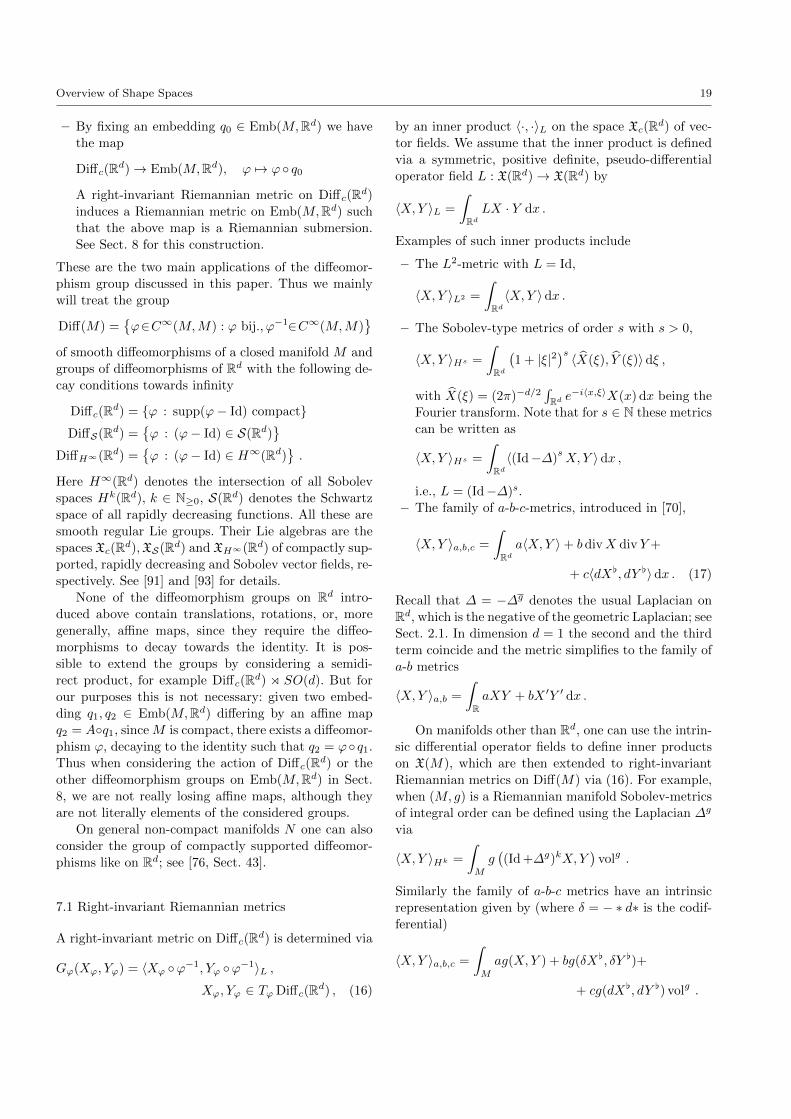
Overview of Shape Spaces 19
– By fixing an embedding q0 ∈ Emb(M,Rd) we have
the map
Diffc(Rd)→ Emb(M,Rd), ϕ 7→ ϕ q0
A right-invariant Riemannian metric on Diffc(Rd)induces a Riemannian metric on Emb(M,Rd) such
that the above map is a Riemannian submersion.
See Sect. 8 for this construction.
These are the two main applications of the diffeomor-
phism group discussed in this paper. Thus we mainly
will treat the group
Diff(M) =ϕ∈C∞(M,M) : ϕ bij.,ϕ−1∈C∞(M,M)
of smooth diffeomorphisms of a closed manifold M and
groups of diffeomorphisms of Rd with the following de-
cay conditions towards infinity
Diffc(Rd) = ϕ : supp(ϕ− Id) compactDiffS(Rd) =
ϕ : (ϕ− Id) ∈ S(Rd)
DiffH∞(Rd) =
ϕ : (ϕ− Id) ∈ H∞(Rd)
.
Here H∞(Rd) denotes the intersection of all Sobolev
spaces Hk(Rd), k ∈ N≥0, S(Rd) denotes the Schwartz
space of all rapidly decreasing functions. All these are
smooth regular Lie groups. Their Lie algebras are the
spaces Xc(Rd),XS(Rd) and XH∞(Rd) of compactly sup-
ported, rapidly decreasing and Sobolev vector fields, re-
spectively. See [91] and [93] for details.
None of the diffeomorphism groups on Rd intro-
duced above contain translations, rotations, or, more
generally, affine maps, since they require the diffeo-
morphisms to decay towards the identity. It is pos-
sible to extend the groups by considering a semidi-
rect product, for example Diffc(Rd) o SO(d). But for
our purposes this is not necessary: given two embed-
ding q1, q2 ∈ Emb(M,Rd) differing by an affine map
q2 = Aq1, sinceM is compact, there exists a diffeomor-
phism ϕ, decaying to the identity such that q2 = ϕ q1.
Thus when considering the action of Diffc(Rd) or the
other diffeomorphism groups on Emb(M,Rd) in Sect.
8, we are not really losing affine maps, although they
are not literally elements of the considered groups.
On general non-compact manifolds N one can also
consider the group of compactly supported diffeomor-
phisms like on Rd; see [76, Sect. 43].
7.1 Right-invariant Riemannian metrics
A right-invariant metric on Diffc(Rd) is determined via
Gϕ(Xϕ, Yϕ) = 〈Xϕ ϕ−1, Yϕ ϕ−1〉L ,Xϕ, Yϕ ∈ Tϕ Diffc(Rd) , (16)
by an inner product 〈·, ·〉L on the space Xc(Rd) of vec-
tor fields. We assume that the inner product is defined
via a symmetric, positive definite, pseudo-differential
operator field L : X(Rd)→ X(Rd) by
〈X,Y 〉L =
∫RdLX · Y dx .
Examples of such inner products include
– The L2-metric with L = Id,
〈X,Y 〉L2 =
∫Rd〈X,Y 〉dx .
– The Sobolev-type metrics of order s with s > 0,
〈X,Y 〉Hs =
∫Rd
(1 + |ξ|2
)s 〈X(ξ), Y (ξ)〉dξ ,
with X(ξ) = (2π)−d/2∫Rd e
−i〈x,ξ〉X(x) dx being the
Fourier transform. Note that for s ∈ N these metrics
can be written as
〈X,Y 〉Hs =
∫Rd〈(Id−∆)
sX,Y 〉dx ,
i.e., L = (Id−∆)s.
– The family of a-b-c-metrics, introduced in [70],
〈X,Y 〉a,b,c =
∫Rda〈X,Y 〉+ bdivX div Y+
+ c〈dX[, dY [〉dx . (17)
Recall that ∆ = −∆g denotes the usual Laplacian on
Rd, which is the negative of the geometric Laplacian; see
Sect. 2.1. In dimension d = 1 the second and the third
term coincide and the metric simplifies to the family of
a-b metrics
〈X,Y 〉a,b =
∫RaXY + bX ′Y ′ dx .
On manifolds other than Rd, one can use the intrin-
sic differential operator fields to define inner products
on X(M), which are then extended to right-invariant
Riemannian metrics on Diff(M) via (16). For example,
when (M, g) is a Riemannian manifold Sobolev-metrics
of integral order can be defined using the Laplacian ∆g
via
〈X,Y 〉Hk =
∫M
g((Id +∆g)kX,Y
)volg .
Similarly the family of a-b-c metrics have an intrinsic
representation given by (where δ = − ∗ d∗ is the codif-
ferential)
〈X,Y 〉a,b,c =
∫M
ag(X,Y ) + bg(δX[, δY [)+
+ cg(dX[, dY [) volg .
20 Martin Bauer et al.
More general Sobolev spaces Hs(M) with s /∈ N and
the corresponding norms can be introduced using parti-
tions of unity and Riemannian exponential coordinates.
See the books [127] and [45] for the theory of function
spaces, including Sobolev spaces of fractional order, on
manifolds.
Remark 7.1 An alternative approach to induce a metric
on the diffeomorphism group is to use a reproducing
kernel Hilbert space H of vector fields, with X(Rd) ⊂ Hand consider the restriction of the inner product on Hto X(Rd). This approach is described in Sect. 8.2.
7.2 Geodesic Equation
The geodesic equation on any Lie group G with a right-
invariant metric is given as follows. A curve g(t) ∈ Gis a geodesic if the right logarithmic derivative u(t) =
∂tg(t)g(t)−1 satisfies
∂tu = − adTu u ,
where adT is the transpose of ad with respect to the
given inner product γ(·, ·) on the Lie algebra, i.e.,
γ(adTu v, w) = γ(v, adu w)
On Diff(Rd) with a metric given via an operator
field L we can write the equation as a PDE in terms of
the momentum m = Lu,
∂tm+(u·∇)m+mdiv u+DuT .m = 0, m = Lu , (18)
and ∂tϕ = u ϕ. For different choices of L one can
obtain the following PDEs as geodesic equations.
The L2-metric with Lu = u in one dimension has as
geodesic equation Burgers’ equation,
ut + 3uux = 0 .
This equation was used as a model equation for turbu-
lence in [24].
The H1-metric with Lu = u−uxx in one dimension
has as geodesic equation the Camassa-Holm equation
[25],
ut − uxxt + 3uux − 2uxuxx − uuxxx = 0 .
It describes the propagation of shallow water waves on
the free surface under gravity. It is a completely inte-
grable equation and possesses a bihamiltonian struc-
ture, that gives rise to an infinite number of conserva-
tion laws.
The homogeneous H1 semi-metric on Diff(S1) with
the operator Lu = −uxx descends to a metric on the
right coset space Rot(S1)\Diff(S1) of diffeomorphisms
modulo rigid rotations. The geodesic equation is the
periodic Hunter-Saxton equation
uxxt + 2uxuxx + uuxxx = 0 .
The Hunter-Saxton equation was proposed as a model
for the propagation of orientation waves in nematic liq-
uid crystals in [60]. Its geodesic nature was discovered
in [72]. It is also a completely integrable, bihamilto-
nian equation with an infinite number of conservation
laws [61]. As a Riemannian manifold (Diff(S1), H1) is
isometric to an open subset of a sphere and as such
has positive constant curvature [80]. It was shown re-
cently in [9], that a related result also holds for the non-
periodic Hunter-Saxton equation, which is the geodesic
equation for the H1-metric on a certain extension of
Diffc(R).
Between the Hunter-Saxton and the Camassa-Holm
equation lies the µ-Hunter-Saxton equation,
uxxt − 2µ(u)ux + 2uxuxx + uuxxx = 0 ,
which is the geodesic equation on the circle with re-
spect to the µH1-metric defined by the operator Lu =
µ(u)− uxx, with µ(u) = 12π
∫S1 udx being the mean. It
was introduced in [69] as a non degenerate metric on
Diff(S1), such that the projection
(Diff(S1), µH1)→ (Rot(S1)\Diff(S1), H1)
is a Riemannian submersion. It is also a completely in-
tegrable, bihamiltonian equation.
The geodesic equation for the homogeneous H1/2-
metric is the modified Constantin-Lax-Majda (mCLM)
equation,
mt + umx + 2uxm = 0, m = Hux .
The mCLM equation is part of a family of one dimen-
sional models for the vorticity equation [37, 40, 107].
Its geodesic nature was recognized in [132]. As for the
Hunter-Saxton equation we have to regard the mCLM
equation on the coset space Rot(S1)\Diff(S1).
In the context of hydrodynamics a closely related
space is the Virasoro-Bott group
Vir(S1) = Diff(S1)×c R ,
with the group operations(ϕ
α
)(ψ
β
)=
(ϕ ψ
α+ β + c(ϕ,ψ)
),
(ϕ
α
)−1
=
(ϕ−1
−α
)for ϕ,ψ ∈ Diff(S1), and α, β ∈ R. The Virasoro-Bott
group is a central extension of Diff(S1) with respect to
the Bott-cocycle:
c : Diff(S1)×Diff(S1)→ R
c(ϕ,ψ) =1
2
∫log(ϕ′ ψ)d logψ′ ,
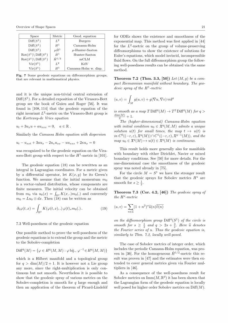
Overview of Shape Spaces 21
Space Metric Geod. equation
Diff(S1) L2 Burgers
Diff(S1) H1 Camassa-Holm
Diff(S1) µH1 µ-Hunter-Saxton
Rot(S1)\Diff(S1) H1 Hunter-Saxton
Rot(S1)\Diff(S1) H1/2 mCLM
Vir(S1) L2 KdV
Vir(S1) H1 Camassa-Holm w. disp.
Fig. 7 Some geodesic equations on diffeomorphism groups,that are relevant in mathematical physics.
and it is the unique non-trivial central extension of
Diff(S1). For a detailed exposition of the Virasoro-Bott
group see the book of Guieu and Roger [56]. It was
found in [108, 114] that the geodesic equation of the
right invariant L2-metric on the Virasoro-Bott group is
the Korteweg-de Vries equation
ut + 3uxu+ auxxx = 0, a ∈ R .
Similarly the Camassa Holm equation with dispersion
ut − uxxt + 3uux − 2uxuxx − uuxxx + 2κux = 0
was recognized to be the geodesic equation on the Vira-
soro-Bott group with respect to the H1-metric in [101].
The geodesic equation (18) can be rewritten as an
integral in Lagrangian coordinates. For a metric given
by a differential operator, let K(x, y) be its Green’s
function. We assume that the initial momentum m0
is a vector-valued distribution, whose components are
finite measures. The initial velocity can be obtained
from m0 via u0(x) =∫Rd K(x, .)m0(.) and conversely
m0 = Lu0 ⊗ dx. Then (18) can be written as
∂tϕ(t, x) =
∫RdK(ϕ(t, x), .)ϕ(t)∗m0(.) . (19)
7.3 Well-posedness of the geodesic equation
One possible method to prove the well-posedness of the
geodesic equations is to extend the group and the metric
to the Sobolev-completion
Diffq(M) = ϕ ∈ Hq(M,M) : ϕbij., ϕ−1∈Hq(M,M)
which is a Hilbert manifold and a topological group
for q > dim(M)/2 + 1. It is however not a Lie group
any more, since the right-multiplication is only con-
tinuous but not smooth. Nevertheless it is possible to
show that the geodesic spray of various metrics on the
Sobolev-completion is smooth for q large enough and
then an application of the theorem of Picard-Lindelof
for ODEs shows the existence and smoothness of the
exponential map. This method was first applied in [44]
for the L2-metric on the group of volume-preserving
diffeomorphisms to show the existence of solutions for
Euler’s equations, which model inviscid, incompressible
fluid flows. On the full diffeomorphism group the follow-
ing well-posedness results can be obtained via the same
method.
Theorem 7.2 (Thm. 3.3, [50]) Let (M, g) be a com-
pact Riemannian manifold without boundary. The geo-
desic spray of the H1-metric
〈u, v〉 =
∫M
g(u, v) + g(∇u,∇v) volg
is smooth as a map T Diffq(M)→ T 2 Diffq(M) for q >dim(M)
2 + 1.
The (higher-dimensional) Camassa-Holm equation
with initial condition u0 ∈ Xq(M,M) admits a unique
solution u(t) for small times, the map t 7→ u(t) is
in C0((−ε, ε),Xq(M))∩C1((−ε, ε),Xq−1(M)), and the
map u0 ∈ Xq(M) 7→ u(t) ∈ Xq(M) is continuous.
This result holds more generally also for manifolds
with boundary with either Dirichlet, Navier or mixed
boundary conditions. See [50] for more details. For the
one-dimensional case the smoothness of the geodesic
spray was noted already in [75].
For the circle M = S1 we have the stronger result
that the geodesic sprays for Sobolev metrics Hs are
smooth for s ≥ 12 .
Theorem 7.3 (Cor. 4.2, [46]) The geodesic spray of
the Hs-metric
〈u, v〉 =∑n∈Z
(1 + n2)su(n)v(n)
on the diffeomorphism group Diffq(S1) of the circle is
smooth for s ≥ 12 and q > 2s + 3
2 . Here u denotes
the Fourier series of u. Thus the geodesic equation is,
similarly to Thm. 7.2, locally well-posed.
The case of Sobolev metrics of integer order, which
includes the periodic Camassa-Holm equation, was pro-
ven in [36]. For the homogeneous H1/2-metric this re-
sult was proven in [47] and the estimates were then ex-
tended to cover general metrics given via Fourier mul-
tipliers in [46].
As a consequence of the well-posedness result for
Sobolev metrics on Imm(M,Rd) it has been shown that
the Lagrangian form of the geodesic equation is locally
well posed for higher order Sobolev metrics on Diff(M).
22 Martin Bauer et al.
Theorem 7.4 (Thm. 10, [11]) Let (M, g) be a com-
pact Riemannian manifold without boundary and let
k ≥ 1 with k ∈ N. For q > dim(M)2 + 2k+ 1 the geodesic
spray of the Hk-metric is smooth as a map on Diffq(M)
and the geodesic equation has unique local solutions on
Diffq(M).
If the metric is strong enough, it is possible to show
the long-time existence of solutions.
Theorem 7.5 If the Green’s function K of the opera-
tor L inducing the metric is a C1-function, then for any
vector-valued distribution m0, whose components are fi-
nite signed measures, equation (19) with ϕ(0, x) = x
can be solved for all time and the solution is a map
(t 7→ ϕ(t, ·)) ∈ C1(R, C1(Rd,Rd)) .
This result is implicit in the work [129], an explicit
proof can be found in [105]. See also [138].
Remark 7.6 This method of proving well-posedness is
not universally applicable as not all geodesic sprays are
smooth. For example the spray induced by the right-
invariant L2-metric on Diff(S1) is not smooth. More
precisely in [35] it is shown that the exponential map
is not a C1-map from a neighborhood of TId Diffq(S1)
to Diffq(S1) for any q ≥ 2. Nevertheless the geodesic
equation, which is Burgers’ equation in this case, has
solutions t 7→ u(t) for small time with
u ∈ C0((−ε, ε), Hq(S1)) ∩ C1((−ε, ε), Hq−1(S1)),
when u0 ∈ Hq(S1); see [66]. A similar statement holds
for the KdV-equation, which is the geodesic equation
on the Virasoro-Bott group with respect to the right-
invariant L2-metric; see [34].
7.4 Geodesic distance
It was shown in [94] that the geodesic distance on the
group Diffc(M) vanishes for the L2-metric and is posi-
tive for the H1-metric. This naturally raises the ques-
tion, what happens for the Hs-metric with 0 < s < 1.
For M = S1 a complete answer is provided in [6],
whereas for more general manifolds N a partial answer
was given in the articles [6, 8].
Theorem 7.7 (Thm. 3.1, [6, 8]) The geodesic dis-
tance on Diffc(M) induced by the Sobolev-type metric
of order s vanishes
– for s < 12 ,
– for s = 12 , when M = S1 × C with C compact.
The geodesic distance is positive
– for s ≥ 1,
– for s > 12 , when dim(M) = 1.
Remark 7.8 By taking C = point to be the zero di-
mensional manifold, the above theorem provides a com-
plete answer for M = S1: the geodesic distance vanishes
if and only if s ≤ 12 .
Remark 7.9 The H1/2-metric on Diff(S1) is the only
known example, where the geodesic spray is smooth on
the Sobolev-completions Diffq(S1) for all q ≥ 52 and the
geodesic distance vanishes at the same time.
It is shown in [46] that for q > 52 the exponential
map is a local diffeomorphism exp : U ⊆ Hq(R) →Diffq(S1). In particular we have the inequality
LenH1/2
(ϕ) ≥ ‖ exp−1(ϕ(1))‖H1/2
for all paths ϕ : [0, 1]→ exp(Bqε(0)) with ϕ(0) = Id. In
other words we have a lower bound on the length for all
paths, that remain Hq-close to Id. This does not how-
ever imply anything about the geodesic distance, since
a path can have small H1/2-length or equivalently re-
main H1/2-close to Id, but leave the Hq-neighborhood.
Open question. For a Sobolev metric of order s the
behavior of the geodesic distance on Diffc(M) remains
open for
– 12 < s < 1 and dim(N) ≥ 2.
– s = 12 and N 6= S1 ×M , with M compact.
Extrapolating from the known cases, we conjecture the
following result: The geodesic distance induced by the
Sobolev-type metric of order s on Diffc(N) vanishes for
s ≤ 12 and is non-degenerate for s > 1
2 .
A main ingredient for the vanishing result is the follow-
ing property of the geodesic distance on Diffc(N):
Lemma 7.10 Let s ≥ 0. If the geodesic distance on
Diffc(N) for a right-invariant Sobolev Hs-metric van-
ishes for one pair ϕ,ψ ∈ Diffc(N) with ϕ 6= ψ, then the
geodesic distance already vanishes identically on all of
Diffc(N).
This lemma follows from the fact that the set
A =ϕ : distH
s
(Id, ϕ) = 0
is a normal subgroup of Diffc(N) for all s ≥ 0 and
because Diffc(N) is a simple group. Thus, if A contains
any element apart from Id it has to be the whole group.
Remark 7.11 We can also consider the geodesic dis-
tance on the Virasoro-Bott group, which is the one-
dimensional central extension of Diff(S1). There the
geodesic distance vanishes for s = 0, i.e., for the L2-
metric. For s > 12 the geodesic distance cannot vanish
identically. Whether it is point-separating is not known.
Overview of Shape Spaces 23
Open question. For a Sobolev metric of order s the
behavior of the geodesic distance on the Virasoro-Bott
group remains open for 0 < s < 1.
One way to define geodesics is to fix two diffeomor-
phisms ϕ0, ϕ1 and to consider the set
B = ϕ(t) : ϕ(0) = ϕ0, ϕ(1) = ϕ1
of all paths joining them. Geodesics then correspond to
critical points of the energy or equivalently the length
functional restricted to the set B. Vanishing of the geo-
desic distance implies that these functionals have no
global minima. The following theorem shows that for
the L2-metric there are no local minima either.
Theorem 7.12 (Thm 3.1, [22]) Let ϕ(t, x) with t ∈[0, T ] be a path in Diffc(R). Let U be a neighborhood of
ϕ in the space C∞c ([0, T ]×R). Then there exists a path
ψ ∈ U with the same endpoints as ϕ and
E(ψ) < E(ϕ),
where E(.) is the energy w.r.t. the right-invariant L2-
metric.
In the article [22] the result is proven for DiffS(R), but
essentially the same proof works also for Diffc(R).
7.5 Completeness
As a corollary of Thm. 7.5 we obtain the result that the
diffeomorphism group equipped with a metric of high
enough order is geodesically complete:
Theorem 7.13 Let (M, g) be a compact Riemannianmanifold and let Gs be the Sobolev metric of order s.
For s ≥ dim(M)+32 the space
(Diff(M), Gs
)is geodesi-
cally complete.
This result is based on the observation, that for s ≥dim(M)+3
2 the kernel of the operator inducing the metric
Gs is a C1-function.
7.6 Curvature
Denote by γ(·, ·) the inner product on the Lie algebra g
of any Lie group G and let u, v ∈ g be orthonormal vec-
tors. Then the sectional curvature of the plane P (u, v)
in G with respect to the right-invariant metric induced
by γ is given by
k(P (u, v)) =1
4‖ adTv u+ adTu v‖2γ − γ(adTv u, adTu v)
− 3
4‖ adu v‖2γ +
1
2γ(adu v, adTv u− adTu v),
where adT is the transpose of ad with respect to the
given inner product γ inducing the right invariant met-
ric.
For general Sobolev metrics there are no results on
curvature available, but for the family of a-b-c-metrics
(17) on the d-dimensional torus Td, it was shown in [70]
that the curvature assumes both signs.
Theorem 7.14 (Thm. 7.1, [70]) If d ≥ 2 and at
least two of the parameters a, b, c are non-zero, then
the sectional curvature of the a-b-c-metric on Diff(Td)assumes both signs.
In dimension one we have the same behavior for the
family of a-b metrics.
Theorem 7.15 (Sect. 6, [70]) If d = 1 and both pa-
rameters a, b are non-zero, then the sectional curvature
of the a-b-metric on Diff(S1) assumes both signs.
There are two special cases, where the sign of the
curvature is constant. The first is the L2-metric (b = 0)
in one dimension.
Theorem 7.16 (Sect. 5.4, [94]) If d = 1 and b = 0
then the sectional curvature of the plane spanned by
two orthonormal vector fields u, v ∈ X(S1) for the a-
b metric on Diff(S1) is given by
k(P (u, v)) =
∫S1
(uv′ − vu′)2 dx .
In particular the sectional curvature is non-negative.
This does not generalize to higher dimensions. De-
note by Td the flat d-dimensional torus.
Theorem 7.17 (Prop. 7.2, [70]) If d ≥ 2 and b =
c = 0 then then the sectional curvature of the a-b-c
metric on Diff(Td) assumes both signs.
The sectional curvature of the L2-metric has been
calculated for an arbitrary Riemannian manifold N .
The expression for sectional curvature is the sum of a
non-negative term and a term whose sign is indefinite.
Although we conjecture that the statement of Thm.
7.17 extends to arbitrary manifoldsN , this has not been
proven yet.
The second special case is the homogeneous H1-
metric with a = c = 0 for d ≥ 2 and a = 0 for d = 1.
The metric is degenerate on Diff(M), but it induces the
Fisher-Rao metric on the space Diff(M)/Diffµ(M) of
densities. Remarkably the induced metric has constant
sectional curvature.
24 Martin Bauer et al.
Theorem 7.18 (Cor. 3.2, [70]) Let (M, g) be a com-
pact Riemannian manifold. Then the homogeneous H1-
metric
〈u, v〉H1 =
∫M
div(u) div(v) vol(g)
on Diff(M)/Diffµ(M) has constant positive sectional
curvature
k(P (u, v)) =1
Vol(M).
This result is based on the observation, that the H1
metric on Diff(M)/Diffµ(M) is isometric to a sphere
in the Hilbert space L2(M, vol(g)). For M = S1 this
result has been proven already in [80]. Recently it has
been shown that the H1-metric on a certain extension
of Diffc(R) is a flat space in the sense of Riemannian
geometry; see [9].
8 Metrics on shape space induced by Diff(Rd)
In this section we will consider Riemannian metrics on
Be(M,Rd), the space of embedded type M submani-
folds that are induced by the left action of Diff(Rd).Let Diff(Rd) stand for one of the groups Diffc(Rd),DiffS(Rd) or DiffH∞(Rd) described in Sect. 7. We also
relax the assumption on the dimension of M and only
require dim(M) < d. The action is given by
Diff(Rd)×Be(M,Rd) 3 (ϕ,Q) 7→ ϕ(Q) ∈ Be(M,Rd) .
This action is in general not transitive – consider for ex-
ample a knotted and an unknotted circle in R3 – but its
orbits are open subsets of Be(M,Rd). Since the groups
Diffc(Rd), DiffS(Rd) and DiffH∞(Rd) connected and M
is compact, the orbits are the connected components of
Be(M,Rd). For Q ∈ Be(M,Rd) the isotropy group
Diff(Rd)Q = ϕ : ϕ(Q) = Q ,
consists of all diffeomorphisms that map Q to itself.
Thus each orbit Orb(Q) = Diff(Rd).Q can be identified
with the quotient
Be(M,Rd) ⊇ Orb(Q) ∼= Diff(Rd)/Diff(Rd)Q .
Let us take a step backwards and remember that an-
other way to represent Be(M,Rd) was as the quotient
Be(M,Rd) ∼= Emb(M,Rd)/Diff(M) .
The diffeomorphism group Diff(Rd) also acts on the
space Emb(M,Rd) of embeddings, that is parametrized
submanifolds with the action
Diff(Rd)×Emb(M,Rd)3(ϕ, q) 7→ ϕ q ∈ Emb(M,Rd).
This action is generally not transitive either, but has
open orbits as before. For fixed q ∈ Emb(M,Rd), the
isotropy group
Diff(Rd)q =ϕ : ϕ|q(M) ≡ Id
,
consists of all diffeomorphisms that fix the image q(M)
pointwise. Note the subtle difference between the two
groups Diff(Rd)q and Diff(Rd)Q, when Q = q(M). The
former consists of diffeomorphisms that fix q(M) point-
wise, while elements of the latter only fix q(M) as a
set. As before we can identify each orbit Orb(q) =
Diff(Rd).q with the set
Emb(M,Rd) ⊇ Orb(q) ∼= Diff(Rd)/Diff(Rd)q .
The isotropy groups are subgroups of each other
Diff(Rd)q E Diff(Rd)Q ≤ Diff(Rd) ,
with Diff(Rd)q being a normal subgroup of Diff(Rd)Q.
Their quotient can be identified with
Diff(Rd)Q/Diff(Rd)q ∼= Diff(M) .
Now we have the two-step process,
Diff(Rd)→→ Diff(Rd)/Diff(Rd)q ∼= Orb(q) ⊆ Emb(M,Rd)→
→ Emb(M,Rd)/Diff(M) ∼= Be(M,Rd) .
In particular the open subset Orb(Q) of Be(M,Rd) can
be represented as any of the quotients
Orb(Q) ∼= Orb(q)/Diff(M) ∼=
∼= Diff(Rd)/Diff(Rd)q/
Diff(Rd)Q/Diff(Rd)q∼=
∼= Diff(Rd)/Diff(Rd)Q .
Let a right-invariant Riemannian metric GDiff be
given on Diff(Rd). Then we can attempt to define a
metric on Emb(M,Rd) in the following way: fix q0 ∈Emb(M,Rd) and let q = ϕ q0 be an element in the
orbit of q0. Define the (semi-)norm of a tangent vector
h ∈ Tq Emb(M,Rd) by
GEmbq (h, h) = inf
Xϕ q0=hGDiffϕ (Xϕ, Xϕ) ,
with Xϕ ∈ Tϕ Diff(Rd). If we define πq0 to be the pro-
jection
πq0 : Diff(Rd)→ Emb(M,Rd), πq0(ϕ) = ϕ q0 ,
then
h = Xϕ q0 = Tϕπq0 .Xϕ ,
Overview of Shape Spaces 25
and the equation defining GEmb is the relation between
two metrics that are connected by a Riemannian sub-
mersion. Because GDiff is right-invariant and the group
action is associative we can rewrite the defining equa-
tion as
GEmbq (h, h) = inf
X q=hGDiff
Id (X,X) ,
with X ∈ TId Diff(Rd). Thus we see that GEmb does not
depend on the choice of q0.
One has to prove in each example, that GEmb is
smooth and a metric, i.e., that it is non-degenerate. We
will see for landmark matching in Sect. 9, that even
though the metric GDiff on Diff(Rd) is smooth, the in-
duced metric on the landmark space Ln(Rd) has only
finitely many derivatives.
While πq0 is a Riemannian submersion this is an
example, where the horizontal bundle exists only in a
suitable Sobolev-completion; see Sect. 2.2. In Sect. 8.2
we will take care of this by defining the metric via a
reproducing kernel Hilbert space H.
Assuming that this construction yields a Rieman-
nian metric on the space Emb(M,Rd), then this metric
is invariant under reparametrizations, because the left-
action by Diff(Rd) commutes with the right-action by
Diff(M):
GEmbq ϕ(h ϕ, h ϕ) = inf
X q ϕ=h ϕGDiff
Id (X,X) =
= infX q=h
GDiffId (X,X) = GEmb
q (h, h) .
The metric GEmb then projects to a Riemannian metric
on Be(M,Rd) as explained in Sect. 2.2.
8.1 Pattern theory
This section is closely related to ideas in Grenander’s
pattern theory [54, 55, 104]. The principle underlying
pattern theory is to explain changes of shape by a de-
formation group acting on the shape. In our case shapes
are elements of either Emb(M,Rd) or Be(M,Rd) and
the deformation group is the group Diff(Rd).There is a lot of flexibility in the choice of the group
and the space it acts upon. If M is a finite set of n
points, then Emb(M,Rd) ⊆ (Rd)n is the set of land-
marks. We have inclusion instead of equality because
landmarks have to be distinct points. We will return to
this space in Sect. 9.
An important example is when the shape space is
the space of volumetric grey-scale images modeled as
functions in C∞(Rd,R) and the deformation group is
Diff(Rd). The action is given by
Diff(Rd)× C∞(Rd,R)3(ϕ, I) 7→ I ϕ−1 ∈ C∞(Rd,R).
This action is far from being transitive. Thus it is not
possible to rigorously define a Riemannian metric on
C∞(Rd,R) that is induced by Diff(Rd). Nevertheless
the idea of images being deformed by diffeomorphisms
led to the image registration method known as LD-
DMM [16, 97, 98, 128]. It is being applied in computa-
tional anatomy with images being MRI and CT scans
to study the connections between anatomical shape and
physiological function. See [23] for an overview of image
registration within the LDDMM framework.
8.2 Defining metrics on Diff(Rd)
Following the presentation in [88] we assume that the
inner product on Xc(Rd) is given in the following way:
let (H, 〈·, ·〉H) be a Hilbert space of vector fields, such
that the canonical inclusions in the following diagram
Xc(Rd) → H → Ckb (Rd,Rd)
are bounded linear mappings for some k ≥ 0. We shall
also assume that the Lie algebra Xc(Rd) of Diff(Rd) is
dense in H. Here Ckb (Rd,Rd) is the space of all glob-
ally bounded Ck-vector fields with the norm ‖X‖k,∞ =∑0≤j≤k ‖DjX‖∞.
Given these assumptions, the space H is a repro-
ducing kernel Hilbert space, i.e., for all x, a ∈ Rd the
directional point-evaluation evax : H → R defined as
evax(u) = 〈u(x), a〉 is a continuous linear functional on
H. See [2] or [112] for a detailed treatment. The relation
〈u,K(., x)a〉H = 〈u(x), a〉
defines a matrix-valued function K : Rd × Rd → Rd×d,called the kernel of H. It satisfies the two properties
– K ∈ Ckb (Rd × Rd,Rd×d) and
– K(y, x) = K(x, y)T .
Associated to H we have the canonical isomorphism
L : H → H∗. Note that the kernel satisfies K(y, x)a =
L−1(evax)(y); this relation is even more general: the
space Mk(Rd,Rd) of vector-valued distributions, whose
components are k-th derivatives of finite signed mea-
sures is a subspace of the dual space Ckb (Rd,Rd)∗ and
the operator
K : Mk(Rd,Rd)→ Ckb (Rd,Rd), m 7→∫RdK(., x)m(x)
coincides with L−1. This is represented in the diagram
Xc(Rd)∗ H∗oo Mk(Rd)oo
K
⊆ // Ckb (Rd,Rd)∗
Xc(Rd) // H //
L
OO
Ckb (Rd,Rd)
26 Martin Bauer et al.
Here Xc(Rd)∗ denotes the space of vector-valued distri-
butions dual to X(Rd), depending on the decay condi-
tions chosen. The inner product on Xc(Rd) is the re-
striction of the inner product on H,
〈X,Y 〉H =
∫Rd〈LX, Y 〉dx ,
where the expression on the right hand side is a sugges-
tive way to denote the pairing 〈LX, Y 〉X∗c×Xc between
a distribution and a vector field.
Example 8.1 LetH = Hk(Rd,Rd) be the Sobolev space
of order k > d2 with the inner product
〈X,Y 〉Hk =
∫Rd〈(Id−∆)kX,Y 〉dx .
Then by the Sobolev embedding theorem we have
Hk(Rd,Rd) → Clb(Rd,Rd) for l < k − d/2.
In this example L : Hk(Rd,Rd) → H−k(Rd,Rd) is the
operator L = (Id−∆)k and the kernel K is the Green’s
function of L,
K(x, y) = (2π)−d/221−k
(k − 1)!|x−y|k−
d2 J
k−d2(|x−y|) Id .
Jα(x) is the modified Bessel function of order α. Around
x = 0 the Bessel function behaves like Jα(|x|) ∼ |x|αand so
|x−y|k−d2 J
k−d2(|x−y|) ∼ |x−y|2k−d around x−y = 0 .
Thus K ∈ C2k−d−1b (Rd×Rd,Rd×d); this will be relevant
in the case of landmarks.
In the above example L was a scalar differential op-
erator; it acted on each component of the vector field
equally and was a multiple of the identity matrix. This
is not always the case. For example the operator asso-
ciated to the family of a-b-c-metrics is in general not
scalar and the corresponding kernel is a dense (not
sparse) matrix.
In Sect. 7 the metric on Diff(Rd) was introduced by
choosing a differential operator. Given an operator with
appropriate properties, it is possible to reconstruct the
space H. The reason for emphasizing the space H and
the reproducing kernel is twofold: Firstly, the induced
metrics on Emb(M,Rd) and the space of landmarks
have a simpler representation in terms of the kernel.
Secondly, in the literature on LDDMM (e.g., in [138])
the starting point is the space H of vector fields and by
presenting both approaches we show their similarities.
8.3 The metric on Emb(M,Rd)
Let GH be a right-invariant metric on Diff(Rd). The
induced metric on Emb(M,Rd) is defined via
GHq (h, h) = infX q=h
〈X,X〉H .
To compute a more explicit expression for GHq , we de-
compose H into
Hvertq = X : X|q ≡ 0 , Hhor
q = (Hvertq )⊥ .
Then the induced metric is
GHq (h, h) = 〈Xhor, Xhor〉H ,
with X ∈ Xc(Rd) any vector field such that X q = h.
The horizontal projection does not depend on the choice
of the lift, i.e., if X,Y ∈ Xc(Rd) coincide along q, then
Xhor = Y hor. We identifyHhorq with the GH-completion
of the tangent space Tq Emb(M,Rd). There are maps
Tq Emb(M,Rd)→ Hhorq
h 7→ Xhor ,Hhorq → Ckb (M,Rd)X 7→ X q .
The composition of these two maps is the canonical
embedding Tq Emb(M,Rd) → Ckb (M,Rd). The space
Hhorq is again a reproducing kernel Hilbert space with
the kernel given by
Kq : M ×M → Rd×d , Kq(x, y) = K(q(x), q(y)) .
Thus we have identified the induced Riemannian metricGH on Emb(M,Rd) as
GHq (h, h) = 〈h, h〉Hhorq.
In this formula we identified Hhorq with vector fields on
M with values in Rd.
8.4 Geodesic distance
If the metric on Diff(Rd) is strong enough, then the in-
duced Riemannian metric on Emb(M,Rd) has a point-
separating geodesic distance function and we conjecture
that the same is true for Be(M,Rd).
Theorem 8.2 If the norm on H is at least as strong
as the C0b -norm. i.e., H → C0
b , then there exists C > 0
such that for q0, q1 ∈ Emb(M,Rd) we have
‖q0 − q1‖∞ ≤ C distHEmb(q0, q1) .
Overview of Shape Spaces 27
Proof Since H → C0b , there exists a constant C > 0,
such that ‖X‖∞ ≤ C‖X‖H holds for all X ∈ H. Given
h ∈ Emb(M,Rd) and x ∈ M let X ∈ X(Rd) be any
vector field with X q = h. From
|h(x)| = |X(q(x))| ≤ ‖X‖∞ ≤ C‖X‖H ,
we see that ‖h‖∞ ≤ C‖X‖∞ and by taking the infimum
over all X we obtain
‖h‖2∞ ≤ C2GHq (h, h) .
Now for any path q(t) between q0 and q1 we have
q1(x)− q0(x) =
∫ 1
0
∂tq(t, x) dt ,
and thus
|q1(x)− q0(x)| ≤∫ 1
0
|∂tq(t, x)|dt ≤
≤ C∫ 1
0
√GHq(t)(∂tq(t), ∂tq(t)) dt = C LenHEmb(q) .
By taking the supremum over x ∈M and the infimum
over all paths we obtain
‖q0 − q1‖∞ ≤ C distLEmb(q0, q1)
as required. ut
For the geodesic distance on shape space we have a
positive result for the space Be(S1,R2) of plane curves
and the family H = Hk(Rd) of Sobolev spaces. A lower
bound on distLBe is given by the Frechet distance (9).
Theorem 8.3 The geodesic distance on Be(S1,R2) of
the outer metric induced by H = Hk(Rd) with the op-
erator L = (1− A∆)k for A > 0 and k ≥ 1 is bounded
from below by the Frechet distance, i.e., for Q0, Q1 ∈Be(S
1,R2) we have
distL∞
Be (Q0, Q1) ≤ distHk
Be (Q0, Q1) .
Proof Take Q0, Q1 ∈ Be(M,Rd) and let Q(t) be a path
between them. Then by [91, Prop. 5.7] we can lift this
path to a horizontal path q(t) on Emb(S1,R2). Then
distL∞
Be (Q0, Q1) ≤ ‖q(0)− q(1)‖∞ =
= LenEmb(q) = LenBe(Q) ,
and by taking the infimum over all paths we obtain the
result. ut
In order to generalize this result to Be(M,Rd) one
would need to be able to lift horizontal paths from
Be(M,Rd) to Emb(M,Rd). A careful analysis of the
induced metric GH in the spirit of [91] should provide
such a result for a fairly general Sobolev-type metric.
8.5 Geodesic equation
The geodesic equation on Emb(M,Rd) is most conve-
niently written in Hamiltonian form in terms of the
position q(t) and the momentum p(t) = p(t) ⊗ volg,
where volg = vol(g) = vol(q∗g). The momentum de-
fines a vector-valued distribution with support in the
image of q(t). The momentum p acts on X ∈ X(Rd) by∫M
〈X q(t), p(t)〉 =
∫M
〈X(q(t, x)), p(t, x)〉 volg(x).
Let us introduce the notation
K ′q(t)(x, y) = D1K(q(t, x), q(t, y))
for the derivative of the kernel with respect to the first
variable. The geodesic equation is given by
∂tq(t, x) = X(t, q(t, x))
∂t (p(t)⊗ volg) (t, x) =
= −(∫
M
p(t, x)TK ′q(t)(x, y)p(t, y) volg(y)
)⊗ volg(x)
X(t, u) =
∫M
K(u, q(t, y))p(t, y) volg(y) .
See [91] for a derivation of the geodesic equation for
plane curves and [88] for the related geodesic equation
on Be(M,Rd).The vector field X is not smooth but only X ∈ H.
Therefore it is not possible to horizontally lift geode-
sics from Emb(M,Rd) to Diff(Rd). One can however
work in a suitable Sobolev completion of Diff(Rd). Then
right-invariance of the Riemannian metric on Diff(Rd)implies the conservation of the momentum:
ϕ(t)∗p(t, .) is independent of t .
From here we obtain via p(t, .) = ϕ(t)∗p(0, .) that ϕ(t)
satisfies the following form of the Euler-Poincare equa-
tion on the diffeomorphism group (EPDiff),
∂tϕ(t, x) =
∫M
K(ϕ(t, x), .)ϕ(t)∗p(0, .) . (20)
See [59] for details on singular solutions of the EPDiff
equations. Theorem 7.5 can be applied to show long-
time existence of solutions of (20).
8.6 Curvature
The representation of Be(M,Rd) as the quotient
Be(M,Rd) = Diff(Rd)/Diff(Rd)Q
was used in [88] together with an infinite dimensional
version of O’Neil’s formula to compute an expression
for the sectional curvature on Be(M,Rd). For details
consult [88, Sect. 5].
28 Martin Bauer et al.
9 The space of landmarks
By choosing M to be the finite set M = 1, . . . , n we
obtain as Emb(M,Rd) the set of landmarks, i.e., the set
of n distinct, labeled points in Rd. Let us denote this
space by
Ln(Rd) :=
(q1, . . . , qn)|qk ∈ Rd, qk 6= qj , k 6= j.
Note that Ln(Rd) is an open subset of Rnd and thus it is
the first example of a finite dimensional shape space in
this paper. As a consequence some of the questions dis-
cussed for other shape spaces have a simple answer for
the space of landmarks. The geodesic distance is guar-
anteed to be point-separating, the geodesic equation is
an ODE and therefore locally well-posed and due to
Hopf-Rinow geodesic completeness implies metric com-
pleteness.
Remark 9.1 We regard landmark space as the set of all
labeled collections of n points in Rd, i.e., the landmarks
q = (q1, q2, . . . qn), q = (q2, q1, . . . qn) are regarded as
different elements of Ln(Rd). One could also consider
the space of unlabeled landmarks Lnu(Rd), which would
correspond to Be(M,Rd). It is sometimes called also
configuration space. Since Diff(M) = Sn is the symmet-
ric group of n elements, we have Lnu(Rd) = Ln(Rd)/Sn.
The group Sn is a finite group, therefore the projec-
tion Ln(Rd) → Lnu(Rd) is a covering map and so for
local properties of Riemannian geometry it is enough
to study the space Ln(Rd).
Before we proceed we need to fix an ordering for
the coordinates on Rnd. There are two canonical choices
and we will follow the convention of [63]. A landmarkq is a vector q = (q1, . . . , qn)T ∈ Ln(Rd) and each qi
has d components qi = (qi1, . . . , qid)T . We concatenate
these vectors as follows
q = (q11, . . . , q1d, q21, . . . , q2d, . . . , qnd)T . (21)
Riemannian metrics on Ln(Rd), that are induced
by the action of the diffeomorphism group, have been
studied in [63, 82, 87] and on the landmark space on
the sphere in [53]. Other metrics on landmark space
include Bookstein’s thin-plate spline distance [19, 20]
and Kendall’s similitude invariant distance [67]. See [97]
for an overview comparing the different approaches.
9.1 A metric on Ln(Rd) induced by Diff(Rd)
As in Sect. 8.2 let the metric GH on Diff(Rd) be defined
via a Hilbert space H of vector fields satisfying the con-
ditions given in Sect. 8.2 and let K be the reproducing
kernel of H. As before we will write Diff(Rd) for any
of the groups Diffc(Rd), DiffS(Rd) or DiffH∞(Rd). The
metric GH induces a Riemannian metric gH on Ln(Rd)and we can calculate it explicitly; see Thm 9.3.
For the convenience of the reader we will repeat the
definition of the distance function on Ln(Rd) induced
by the metric GH; see Sect. 8 for the the more general
situation of embeddings of an arbitrary manifold M in
Rd. Let E be the energy functional of the metric GH
on the diffeomorphism group, i.e.,
E(v) =
∫ 1
0
‖v(t, ·)‖2H dt . (22)
The induced distance function of the action of the dif-
feomorphism group on the landmark space is given by
distH(q, q) = infv
√E(v) : ϕv(qi) = qi
, (23)
where ϕv is the flow of the time dependent vector field
v and where the infimum is taken over all sufficiently
smooth vector fields v : [0, 1] → X(Rd). Given a solu-
tion v of the above minimization problem, the landmark
trajectories qi(t) are then given as the solutions of the
ODE
qi(t) = v(t, qi(t)), i = 1 . . . , n .
We will now define a Riemannian metric on the fi-
nite dimensional space Ln(Rd) directly and we will see
that it is in fact induced by the metric GH on the dif-
feomorphism group. For a landmark q we define the
matrix
g−1H (q) =
K(q1, q1) · · · K(q1, qn)...
. . ....
K(qn, q1) · · · K(qn, qn)
∈ Rnd×nd , (24)
where K : Rd×Rd → Rd×d is the kernel of H. That gHdefines a Riemannian metric on Ln(Rd) can be easily
shown using the properties of the kernel K.
The metric gH defines, in the usual way, an energy
functional directly on the space of landmark trajecto-
ries,
E(q(t)) =
∫ 1
0
q(t)T gH(q(t))q(t) dt , (25)
and one can also define the induced distance function
of g as
distH(q, q) = infq(t)
√E(q(t)) : q(0) = q, q(1) = q
,
(26)
where the infimum is taken over all sufficiently smooth
paths in landmark space q : [0, 1]→ Ln(Rd).It is shown in [87, Prop. 2] that the minimization
problems (23) and (26) are equivalent and that the in-
duced distance functions are equal:
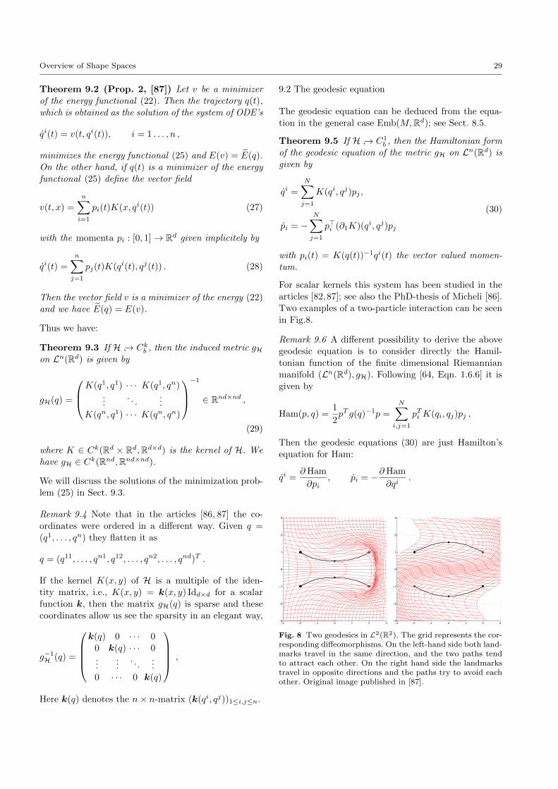
Overview of Shape Spaces 29
Theorem 9.2 (Prop. 2, [87]) Let v be a minimizer
of the energy functional (22). Then the trajectory q(t),
which is obtained as the solution of the system of ODE’s
qi(t) = v(t, qi(t)), i = 1 . . . , n ,
minimizes the energy functional (25) and E(v) = E(q).
On the other hand, if q(t) is a minimizer of the energy
functional (25) define the vector field
v(t, x) =
n∑i=1
pi(t)K(x, qi(t)) (27)
with the momenta pi : [0, 1]→ Rd given implicitely by
qi(t) =
n∑j=1
pj(t)K(qi(t), qj(t)) . (28)
Then the vector field v is a minimizer of the energy (22)
and we have E(q) = E(v).
Thus we have:
Theorem 9.3 If H → Ckb , then the induced metric gHon Ln(Rd) is given by
gH(q) =
K(q1, q1) · · · K(q1, qn)...
. . ....
K(qn, q1) · · · K(qn, qn)
−1
∈ Rnd×nd ,
(29)
where K ∈ Ck(Rd × Rd,Rd×d) is the kernel of H. We
have gH ∈ Ck(Rnd,Rnd×nd).
We will discuss the solutions of the minimization prob-
lem (25) in Sect. 9.3.
Remark 9.4 Note that in the articles [86, 87] the co-
ordinates were ordered in a different way. Given q =
(q1, . . . , qn) they flatten it as
q = (q11, . . . , qn1, q12, . . . , qn2, . . . , qnd)T .
If the kernel K(x, y) of H is a multiple of the iden-
tity matrix, i.e., K(x, y) = k(x, y) Idd×d for a scalar
function k, then the matrix gH(q) is sparse and these
coordinates allow us see the sparsity in an elegant way,
g−1H (q) =
k(q) 0 · · · 0
0 k(q) · · · 0...
.... . .
...
0 · · · 0 k(q)
,
Here k(q) denotes the n× n-matrix (k(qi, qj))1≤i,j≤n.
9.2 The geodesic equation
The geodesic equation can be deduced from the equa-
tion in the general case Emb(M,Rd); see Sect. 8.5.
Theorem 9.5 If H → C1b , then the Hamiltonian form
of the geodesic equation of the metric gH on Ln(Rd) is
given by
qi =
N∑j=1
K(qi, qj)pj ,
pi = −N∑j=1
p>i (∂1K)(qi, qj)pj
(30)
with pi(t) = K(q(t))−1qi(t) the vector valued momen-
tum.
For scalar kernels this system has been studied in the
articles [82,87]; see also the PhD-thesis of Micheli [86].
Two examples of a two-particle interaction can be seen
in Fig.8.
Remark 9.6 A different possibility to derive the above
geodesic equation is to consider directly the Hamil-
tonian function of the finite dimensional Riemannian
manifold (Ln(Rd), gH). Following [64, Eqn. 1.6.6] it is
given by
Ham(p, q) =1
2pT g(q)−1p =
N∑i,j=1
pTi K(qi, qj)pj ,
Then the geodesic equations (30) are just Hamilton’s
equation for Ham:
qi =∂Ham
∂pi, pi = −∂Ham
∂qi.
−3 −2 −1 0 1 2 3−3
−2
−1
0
1
2
3
−3 −2 −1 0 1 2 3−3
−2
−1
0
1
2
3
Fig. 8 Two geodesics in L2(R2). The grid represents the cor-responding diffeomorphisms. On the left-hand side both land-marks travel in the same direction, and the two paths tendto attract each other. On the right hand side the landmarkstravel in opposite directions and the paths try to avoid eachother. Original image published in [87].
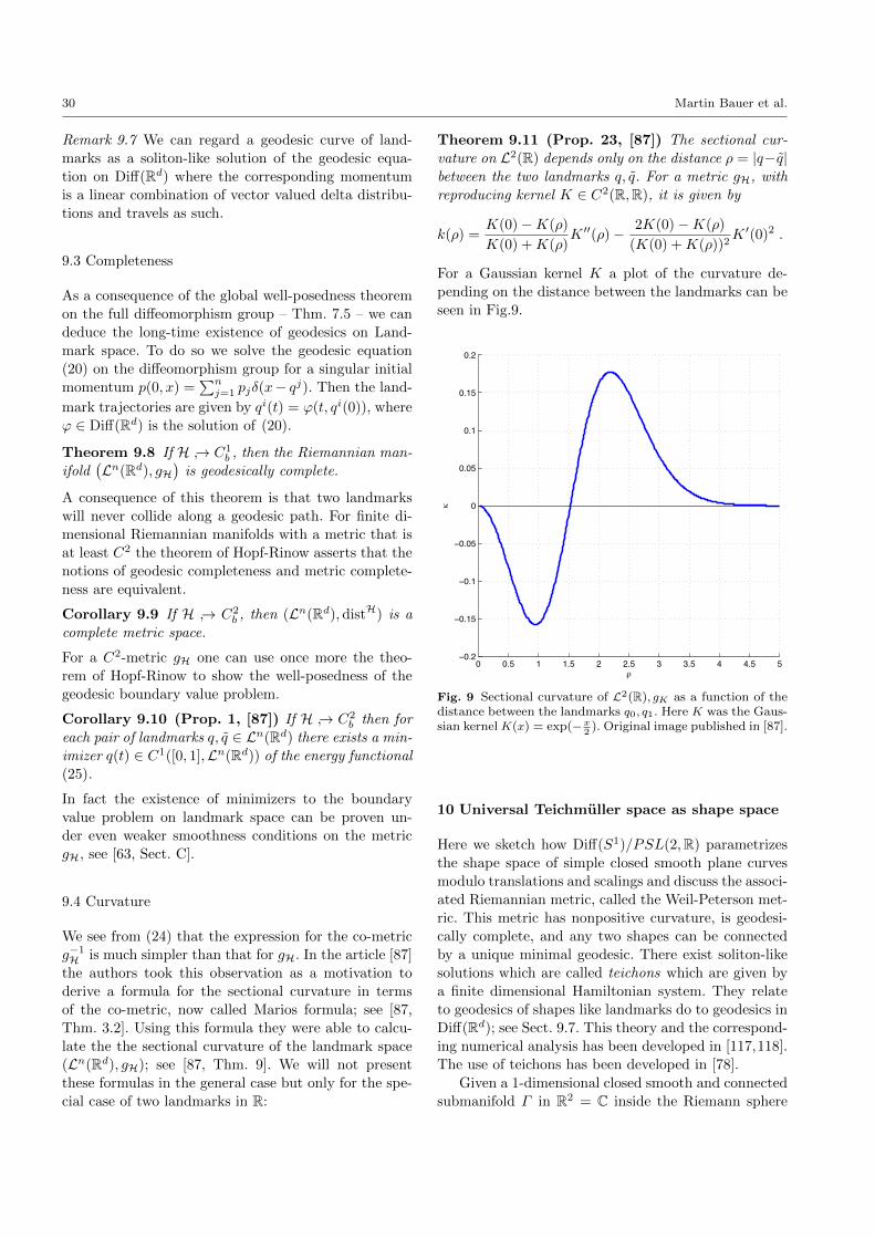
30 Martin Bauer et al.
Remark 9.7 We can regard a geodesic curve of land-
marks as a soliton-like solution of the geodesic equa-
tion on Diff(Rd) where the corresponding momentum
is a linear combination of vector valued delta distribu-
tions and travels as such.
9.3 Completeness
As a consequence of the global well-posedness theorem
on the full diffeomorphism group – Thm. 7.5 – we can
deduce the long-time existence of geodesics on Land-
mark space. To do so we solve the geodesic equation
(20) on the diffeomorphism group for a singular initial
momentum p(0, x) =∑nj=1 pjδ(x− qj). Then the land-
mark trajectories are given by qi(t) = ϕ(t, qi(0)), where
ϕ ∈ Diff(Rd) is the solution of (20).
Theorem 9.8 If H → C1b , then the Riemannian man-
ifold(Ln(Rd), gH
)is geodesically complete.
A consequence of this theorem is that two landmarks
will never collide along a geodesic path. For finite di-
mensional Riemannian manifolds with a metric that is
at least C2 the theorem of Hopf-Rinow asserts that the
notions of geodesic completeness and metric complete-
ness are equivalent.
Corollary 9.9 If H → C2b , then (Ln(Rd),distH) is a
complete metric space.
For a C2-metric gH one can use once more the theo-
rem of Hopf-Rinow to show the well-posedness of the
geodesic boundary value problem.
Corollary 9.10 (Prop. 1, [87]) If H → C2b then for
each pair of landmarks q, q ∈ Ln(Rd) there exists a min-imizer q(t) ∈ C1([0, 1],Ln(Rd)) of the energy functional
(25).
In fact the existence of minimizers to the boundary
value problem on landmark space can be proven un-
der even weaker smoothness conditions on the metric
gH, see [63, Sect. C].
9.4 Curvature
We see from (24) that the expression for the co-metric
g−1H is much simpler than that for gH. In the article [87]
the authors took this observation as a motivation to
derive a formula for the sectional curvature in terms
of the co-metric, now called Marios formula; see [87,
Thm. 3.2]. Using this formula they were able to calcu-
late the the sectional curvature of the landmark space
(Ln(Rd), gH); see [87, Thm. 9]. We will not present
these formulas in the general case but only for the spe-
cial case of two landmarks in R:
Theorem 9.11 (Prop. 23, [87]) The sectional cur-
vature on L2(R) depends only on the distance ρ = |q−q|between the two landmarks q, q. For a metric gH, with
reproducing kernel K ∈ C2(R,R), it is given by
k(ρ) =K(0)−K(ρ)
K(0) +K(ρ)K ′′(ρ)− 2K(0)−K(ρ)
(K(0) +K(ρ))2K ′(0)2 .
For a Gaussian kernel K a plot of the curvature de-
pending on the distance between the landmarks can be
seen in Fig.9.
0 0.5 1 1.5 2 2.5 3 3.5 4 4.5 5−0.2
−0.15
−0.1
−0.05
0
0.05
0.1
0.15
0.2
!
"
Fig. 9 Sectional curvature of L2(R), gK as a function of thedistance between the landmarks q0, q1. Here K was the Gaus-sian kernel K(x) = exp(−x
2). Original image published in [87].
10 Universal Teichmuller space as shape space
Here we sketch how Diff(S1)/PSL(2,R) parametrizes
the shape space of simple closed smooth plane curves
modulo translations and scalings and discuss the associ-
ated Riemannian metric, called the Weil-Peterson met-
ric. This metric has nonpositive curvature, is geodesi-
cally complete, and any two shapes can be connected
by a unique minimal geodesic. There exist soliton-like
solutions which are called teichons which are given by
a finite dimensional Hamiltonian system. They relate
to geodesics of shapes like landmarks do to geodesics in
Diff(Rd); see Sect. 9.7. This theory and the correspond-
ing numerical analysis has been developed in [117,118].
The use of teichons has been developed in [78].
Given a 1-dimensional closed smooth and connected
submanifold Γ in R2 = C inside the Riemann sphere
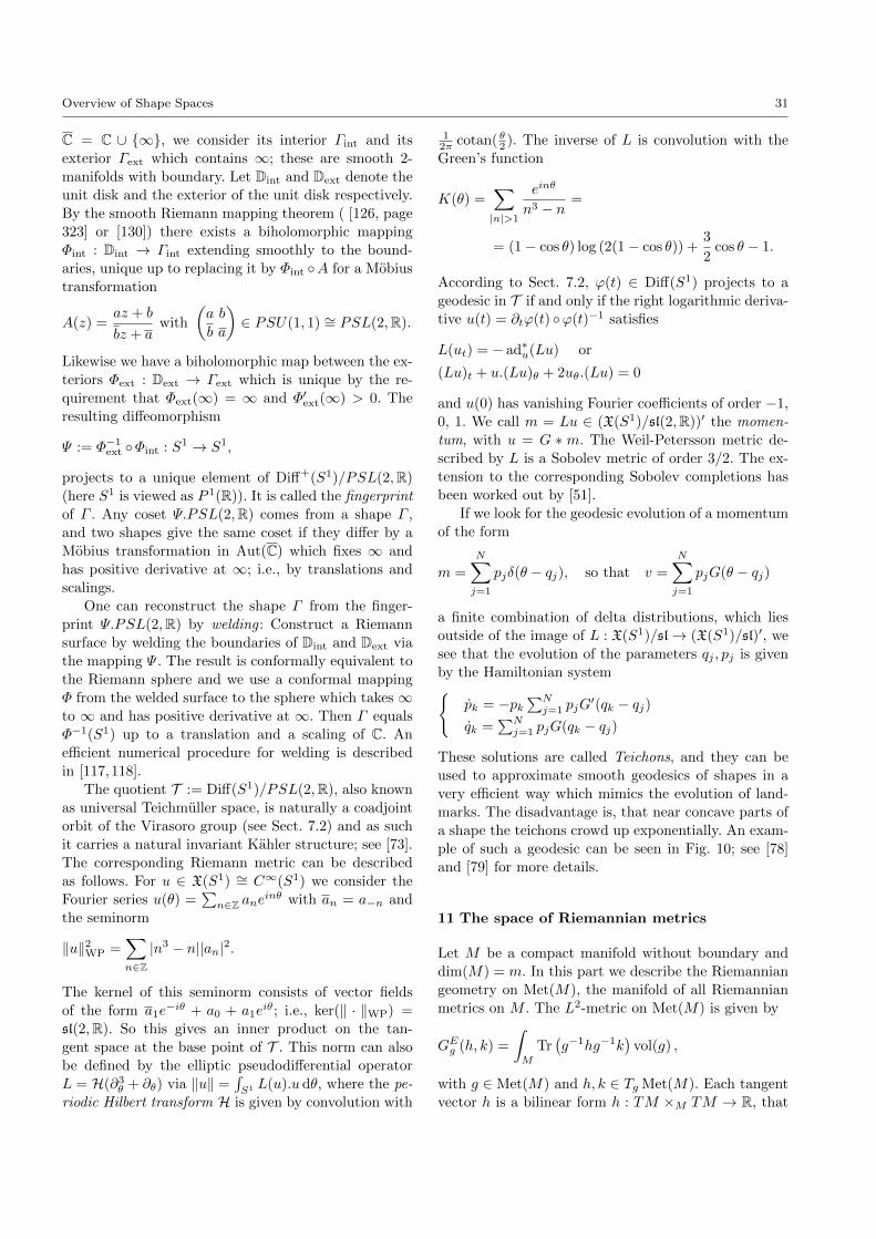
Overview of Shape Spaces 31
C = C ∪ ∞, we consider its interior Γint and its
exterior Γext which contains ∞; these are smooth 2-
manifolds with boundary. Let Dint and Dext denote the
unit disk and the exterior of the unit disk respectively.
By the smooth Riemann mapping theorem ( [126, page
323] or [130]) there exists a biholomorphic mapping
Φint : Dint → Γint extending smoothly to the bound-
aries, unique up to replacing it by Φint A for a Mobius
transformation
A(z) =az + b
bz + awith
(a b
b a
)∈ PSU(1, 1) ∼= PSL(2,R).
Likewise we have a biholomorphic map between the ex-
teriors Φext : Dext → Γext which is unique by the re-
quirement that Φext(∞) = ∞ and Φ′ext(∞) > 0. The
resulting diffeomorphism
Ψ := Φ−1ext Φint : S1 → S1,
projects to a unique element of Diff+(S1)/PSL(2,R)
(here S1 is viewed as P 1(R)). It is called the fingerprint
of Γ . Any coset Ψ.PSL(2,R) comes from a shape Γ ,
and two shapes give the same coset if they differ by a
Mobius transformation in Aut(C) which fixes ∞ and
has positive derivative at ∞; i.e., by translations and
scalings.
One can reconstruct the shape Γ from the finger-
print Ψ.PSL(2,R) by welding : Construct a Riemann
surface by welding the boundaries of Dint and Dext via
the mapping Ψ . The result is conformally equivalent to
the Riemann sphere and we use a conformal mapping
Φ from the welded surface to the sphere which takes∞to ∞ and has positive derivative at ∞. Then Γ equals
Φ−1(S1) up to a translation and a scaling of C. An
efficient numerical procedure for welding is described
in [117,118].
The quotient T := Diff(S1)/PSL(2,R), also known
as universal Teichmuller space, is naturally a coadjoint
orbit of the Virasoro group (see Sect. 7.2) and as such
it carries a natural invariant Kahler structure; see [73].
The corresponding Riemann metric can be described
as follows. For u ∈ X(S1) ∼= C∞(S1) we consider the
Fourier series u(θ) =∑n∈Z ane
inθ with an = a−n and
the seminorm
‖u‖2WP =∑n∈Z|n3 − n||an|2.
The kernel of this seminorm consists of vector fields
of the form a1e−iθ + a0 + a1e
iθ; i.e., ker(‖ · ‖WP) =
sl(2,R). So this gives an inner product on the tan-
gent space at the base point of T . This norm can also
be defined by the elliptic pseudodifferential operator
L = H(∂3θ + ∂θ) via ‖u‖ =
∫S1 L(u).udθ, where the pe-
riodic Hilbert transform H is given by convolution with
12π cotan( θ2 ). The inverse of L is convolution with the
Green’s function
K(θ) =∑|n|>1
einθ
n3 − n=
= (1− cos θ) log (2(1− cos θ)) +3
2cos θ − 1.
According to Sect. 7.2, ϕ(t) ∈ Diff(S1) projects to a
geodesic in T if and only if the right logarithmic deriva-
tive u(t) = ∂tϕ(t) ϕ(t)−1 satisfies
L(ut) = − ad∗u(Lu) or
(Lu)t + u.(Lu)θ + 2uθ.(Lu) = 0
and u(0) has vanishing Fourier coefficients of order −1,
0, 1. We call m = Lu ∈ (X(S1)/sl(2,R))′ the momen-
tum, with u = G ∗ m. The Weil-Petersson metric de-
scribed by L is a Sobolev metric of order 3/2. The ex-
tension to the corresponding Sobolev completions has
been worked out by [51].
If we look for the geodesic evolution of a momentum
of the form
m =
N∑j=1
pjδ(θ − qj), so that v =
N∑j=1
pjG(θ − qj)
a finite combination of delta distributions, which lies
outside of the image of L : X(S1)/sl→ (X(S1)/sl)′, we
see that the evolution of the parameters qj , pj is given
by the Hamiltonian systempk = −pk
∑Nj=1 pjG
′(qk − qj)qk =
∑Nj=1 pjG(qk − qj)
These solutions are called Teichons, and they can be
used to approximate smooth geodesics of shapes in a
very efficient way which mimics the evolution of land-
marks. The disadvantage is, that near concave parts of
a shape the teichons crowd up exponentially. An exam-
ple of such a geodesic can be seen in Fig. 10; see [78]
and [79] for more details.
11 The space of Riemannian metrics
Let M be a compact manifold without boundary and
dim(M) = m. In this part we describe the Riemannian
geometry on Met(M), the manifold of all Riemannian
metrics on M . The L2-metric on Met(M) is given by
GEg (h, k) =
∫M
Tr(g−1hg−1k
)vol(g) ,
with g ∈ Met(M) and h, k ∈ Tg Met(M). Each tangent
vector h is a bilinear form h : TM ×M TM → R, that
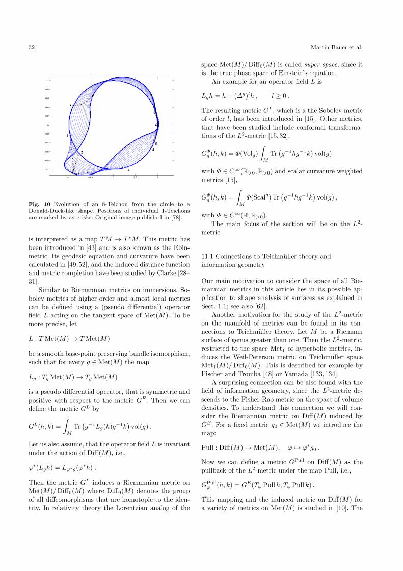
32 Martin Bauer et al.
−1 −0.5 0 0.5 1
−1
−0.8
−0.6
−0.4
−0.2
0
0.2
0.4
0.6
0.8
1
1
2
3
45
6
7
8
Fig. 10 Evolution of an 8-Teichon from the circle to aDonald-Duck-like shape. Positions of individual 1-Teichonsare marked by asterisks. Original image published in [78].
is interpreted as a map TM → T ∗M . This metric has
been introduced in [43] and is also known as the Ebin-
metric. Its geodesic equation and curvature have been
calculated in [49,52], and the induced distance function
and metric completion have been studied by Clarke [28–
31].
Similar to Riemannian metrics on immersions, So-
bolev metrics of higher order and almost local metrics
can be defined using a (pseudo differential) operator
field L acting on the tangent space of Met(M). To be
more precise, let
L : T Met(M)→ T Met(M)
be a smooth base-point preserving bundle isomorphism,
such that for every g ∈ Met(M) the map
Lg : Tg Met(M)→ Tg Met(M)
is a pseudo differential operator, that is symmetric and
positive with respect to the metric GE . Then we can
define the metric GL by
GL(h, k) =
∫M
Tr(g−1Lg(h)g−1k
)vol(g) .
Let us also assume, that the operator field L is invariant
under the action of Diff(M), i.e.,
ϕ∗(Lgh) = Lϕ∗g(ϕ∗h) .
Then the metric GL induces a Riemannian metric on
Met(M)/Diff0(M) where Diff0(M) denotes the group
of all diffeomorphisms that are homotopic to the iden-
tity. In relativity theory the Lorentzian analog of the
space Met(M)/Diff0(M) is called super space, since it
is the true phase space of Einstein’s equation.
An example for an operator field L is
Lgh = h+ (∆g)lh , l ≥ 0 .
The resulting metric GL, which is a the Sobolev metric
of order l, has been introduced in [15]. Other metrics,
that have been studied include conformal transforma-
tions of the L2-metric [15,32],
GΦg (h, k) = Φ(Volg)
∫M
Tr(g−1hg−1k
)vol(g)
with Φ ∈ C∞(R>0,R>0) and scalar curvature weighted
metrics [15],
GΦg (h, k) =
∫M
Φ(Scalg) Tr(g−1hg−1k
)vol(g) ,
with Φ ∈ C∞(R,R>0).
The main focus of the section will be on the L2-
metric.
11.1 Connections to Teichmuller theory and
information geometry
Our main motivation to consider the space of all Rie-
mannian metrics in this article lies in its possible ap-
plication to shape analysis of surfaces as explained in
Sect. 1.1; see also [62].
Another motivation for the study of the L2-metric
on the manifold of metrics can be found in its con-
nections to Teichmuller theory. Let M be a Riemann
surface of genus greater than one. Then the L2-metric,
restricted to the space Met1 of hyperbolic metrics, in-
duces the Weil-Peterson metric on Teichmuller space
Met1(M)/Diff0(M). This is described for example by
Fischer and Tromba [48] or Yamada [133,134].
A surprising connection can be also found with the
field of information geometry, since the L2-metric de-
scends to the Fisher-Rao metric on the space of volume
densities. To understand this connection we will con-
sider the Riemannian metric on Diff(M) induced by
GE . For a fixed metric g0 ∈ Met(M) we introduce the
map:
Pull : Diff(M)→ Met(M), ϕ 7→ ϕ∗g0 .
Now we can define a metric GPull on Diff(M) as the
pullback of the L2-metric under the map Pull, i.e.,
GPullϕ (h, k) = GE(Tϕ Pullh, Tϕ Pull k) .
This mapping and the induced metric on Diff(M) for
a variety of metrics on Met(M) is studied in [10]. The
Overview of Shape Spaces 33
metric GPull is invariant under the left action by the
group Diffµ(M) of volume-preserving diffeomorphisms
and the metric induced on the quotient space
Dens(M) ∼= Diffµ(M)\Diff(M)
of densities is the Fisher-Rao metric; see [102, Thm.
4.9].
Another possibility, to see the connection to infor-
mation geometry was implicitly presented in [33]. There
the authors consider the subspace of Kahler metrics in
a fixed Kahler class – assuming that M admits a Kahler
structure. Then the Ebin metric induces the so-called
Calabi geometry on the space of Kahler metrics. It was
then observed in [71] that this space is, via the Calabi-
Yau map, isometric to the space of volume densities
with the Fisher-Rao metric.
11.2 Geodesic distance
In contrast to to the spaces of immersions, submani-
folds and the diffeomorphism group, the L2-metric on
Met(M) induces a point-separating geodesic distance
function.
Theorem 11.1 (Thm. 18, [29]) The L2-metric in-
duces a point-separating geodesic distance function on
Met(M).
Remark 11.2 Note that this result also holds for all
metrics, that are stronger than the L2-metric, i.e.,
GEg (h, h) ≤ CGg(h, h) ,
with a constant C > 0, independent of g. This applies
in particular to almost local metrics, if the function Φis bounded from below by Φ ≥ C > 0, as well as to
most Sobolev-type metrics.
Fix a Riemannian metric g on M . For each x ∈ Mdenote by Met(M)x = S2
+T∗xM the space of symmet-
ric, positive definite(
02
)-tensors at x. Then for b, c ∈
Ta Met(M)x the expression
γx,a(b, c) = Tr(a−1ba−1c)√
det g(x)−1a
defines a Riemannian metric on the finite-dimensional
manifold Met(M)x. Denote by dx the induced geodesic
distance function and define the following distance on
Met(M),
Ω2(g0, g1) =
√∫M
dx(g0(x), g1(x))2 vol(g) .
The following theorem states that computing the geode-
sic distance on Met(M) with respect to the L2-distance,
is equivalent to summing point-wise geodesic distances
on Met(M)x.
Theorem 11.3 (Thm. 3.8, [32]) Geodesic distance
induced by the L2 metric and the distance Ω2 coincide,
i.e., for all g0, g1 ∈ Met(M),
distE(g0, g1) = Ω2(g0, g1) .
Similar as in the case of the GA-metric and the So-
bolev metrics on the space of immersions the square
root of the volume is again a Lipschitz continuous func-
tion.
Theorem 11.4 (Lem. 12, [29]) Geodesic distance in-
duced by the L2-metric satisfies the inequality∣∣∣√Vol(F, g0)−√
Vol(F, g1)∣∣∣ ≤ √m
4distEMet(M)(g0, g1)
for any measurable set F ⊂M . Here Vol(F, g) denotes
the volume of F ⊂M with respect to the metric g.
This implies the Lipschitz continuity of the map
√Vol :
(Met(M),distFMet(M)
)→ R≥0.
On the other hand we also have the following upper
bound for the geodesic distance.
Theorem 11.5 (Prop. 4.1, [31]) For the L2-metric
the geodesic distance is bounded from above by
distE(g0, g1) ≤ C(m)(√
Vol(F, g0) +√
Vol(F, g1)),
where F denotes the support of g1 − g0
F = x ∈M |g0(x) 6= g1(x) ,
and C(m) is a constant depending only on the dimen-sion of M .
The above corollary implies that the set Metµ(M)
of all Riemannian metrics having a total volume less or
equal than µ has a finite diameter with respect to the
L2-metric.
11.3 The geodesic equation
The Christoffel symbols for the L2-metric were first cal-
culated in [43, Sect. 4]. Subsequently Freed and Groisser
[49] and Michor and Gil-Medrano [52] computed the
geodesic equation and found explicit solution formu-
las. The geodesic equation for higher order Sobolev
type metrics and Scalar curvature metrics can be found
in [15] and for volume weighted metrics in [15,33].
The geodesic equation for the L2-metric decouples
the time and spatial variables, i.e., instead of being a
PDE in (t, x), it is only an ODE in t.
34 Martin Bauer et al.
Lemma 11.6 (Sect. 4, [43]) The geodesic equation
for the L2-metric is given by the ordinary differential
equation:
gtt =1
4Tr(g−1gtg
−1gt)g + gtg−1gt −
1
2Tr(g−1gt)gt .
There exists an explicit solution formula for this ODE.
Theorem 11.7 The geodesic starting at g0 ∈ Met(M)
in the direction of h ∈ Tg0 Met(M) is given by the curve
g(t) = g0ea(t) Id +b(t)H0 ,
where H0 is the traceless part of H := g−10 h, i.e., H0 =
H − Tr(H)m Id, and where a(t) and b(t) ∈ C∞(M) are
defined by
a(t) = 2m log
((1 + t
4 Tr(H))2 + m16 Tr(H2
0 )t2)
b(t) =
4√
mTr(H20 )
arctan
(√mTr(H2
0 ) t
4+tTr(H)
),Tr(H2
0 ) 6= 0
t1+ t
4 Tr(H), Tr(H2
0 ) = 0.
Here arctan is taken to have values in (−π2 ,π2 ) for the
points of the manifold where Tr(H) ≥ 0, and on a point
where Tr(H) < 0 we define
arctan
(√mTr(H2
0 ) t
4 + tTr(H)
)
=
arctan in [0, π2 ) for t ∈ [0,− 4
Tr(H) )π2 for t = − 4
Tr(H)
arctan in (π2 , π) for t ∈ (− 4Tr(H) ,∞).
Let Nh := x ∈ M : H0(x) = 0, and if Nh 6= ∅ let
th := infTr(H)(x) : x ∈ Nh. Then the geodesic g(t)
is defined for t ∈ [0,∞) if Nh = ∅ or if th ≥ 0, and it
is only defined for t ∈ [0,− 4th
) if th < 0.
These formulas have been independently derived by
Freed and Groisser [49] and Michor and Gil-Medrano
[52]. A similar result is also available for the metric GΦ
with Φ(Vol) = 1Vol ; see [33].
Remark 11.8 The geodesic equation for higher order
metrics will generally not be an ODE anymore and ex-
plicit solution formulas do not exist. Nevertheless, it
has been shown that the geodesic equations are (lo-
cally) well-posed, assuming certain conditions on the
operator field L defining the metric; see [15]. These con-
ditions are satisfied by the class of Sobolev type metrics
and conformal metrics but not by the scalar curvature
weighted metrics.
11.4 Conserved quantities
Noether’s theorem associates to any metric on Met(M),
that is invariant under pull-backs by the diffeomor-
phism group Diff(M), for each X ∈ X(M) the quantity
Gg(gt, ζX(g)) = const ,
which is conserved along each geodesic g(t). Here ζXis the fundamental vector field of the right action of
Diff(M),
ζX(g) = LXg = 2 Sym∇g(g(X)) ,
and Sym∇g(g(X)) is the symmetrization of the bilinear
form (Y,Z) 7→ ∇gY g(X,Z), i.e.,
Sym∇g(g(X))(Y,Z) = 12 (∇gY g(X,Z) +∇gZg(X,Y )) .
If Gg(gt, ζX(g)) vanishes for all vector fields X ∈ X(M)
along a geodesic g(t), then g(t) intersects each Diff(M)-
orbit orthogonally.
11.5 Completeness
The L2-metric on Met(M) is incomplete, both metri-
cally and geodesically. The metric completion of it has
been studied by Clarke in [28, 31, 32]. To describe the
completion let Metf denote the set of measurable sec-
tions of the bundle S2≥0T
∗M of symmetric, positive
semi-definite(
02
)-tensors, which have finite total vol-
ume. Define an equivalence relation on Metf by iden-
tifying g0 ∼ g1, if the following statement holds almost
surely:
g0(x) 6= g1(x)⇒ both gi(x) are not positive definite.
In other words, let D = x : g0(x) 6= g1(x) and Ai =
x : gi(x) not pos. def.. Then
g0 ∼ g1 ⇔ D \ (A0 ∩A1) has measure 0 .
Note that the map Met(M) → Metf /∼ is injective.
Theorem 11.9 (Thm. 5.17, [28]) The metric com-
pletion of the space (Met(M),distE) can be naturally
identified with Metf /∼.
In the subsequent article [32] it is shown that the
metric completion is a non-positively curved space in
the sense of Alexandrov.
Theorem 11.10 (Thm 5.6, [32]) The metric com-
pletion Met(M) of Met(M) with respect to the distE-
metric is a CAT(0) space, i.e.,
1. there exists a length-minimizing path (geodesic) be-
tween any two points in Met(M) and
2.(Met(M),distE
)is a non-positively curved space in
the sense of Alexandrov.
Overview of Shape Spaces 35
11.6 Curvature
For the L2-metric, there exists a comparably simple
expression for the curvature tensor.
Theorem 11.11 (Prop. 2.6, [52]) The Riemannian
curvature for the L2–metric on the manifold Met(M)
of all Riemannian metrics is given by
g−1Rg(h, k)l = 14 [[H,K], L]
+m
16(Tr(KL)H − Tr(HL)K)
+1
16(Tr(H) Tr(L)K − Tr(K) Tr(L)H)
+1
16(Tr(K) Tr(HL)− Tr(H) Tr(KL)) Id ,
where H = g−1h, K = g−1k and L = g−1l.
In the article [49] the authors have determined the
sign of the sectional curvature:
Theorem 11.12 (Cor. 1.17, [49]) The sectional cur-
vature for the L2–metric on the manifold Met(M) of
all Riemannian metrics is non-positive. For the plane
P (h, k) spanned by orthonormal h, k it is
kMetg (P (h, k)) =
∫M
m
16
(Tr(HK)2 − Tr(H)2 Tr(K)2
)+
1
4Tr(
([H,K])2)
vol(g) ,
where H = g−1h and K = g−1k.
In [33] it is proven that this negative curvature carries
over to the metric-completion of (Met(M), GE), as it is
a CAT(0) space; see Lem. 11.10.
Acknowledgements We would like to thank the referees fortheir careful reading of the article as well as the thoughtfulcomments, that helped us improve the exposition.
References
1. D. Alekseevsky, A. Kriegl, M. Losik, and P. W. Michor.The Riemannian geometry of orbit spaces—the metric,geodesics, and integrable systems. Publ. Math. Debre-
cen, 62(3-4):247–276, 2003. Dedicated to Professor La-jos Tamassy on the occasion of his 80th birthday.
2. N. Aronszajn. Theory of reproducing kernels. Trans.
Amer. Math. Soc., 68:337–404, 1950.3. M. Bauer. Almost local metrics on shape space of surfaces.
PhD thesis, University of Vienna, 2010.4. M. Bauer and M. Bruveris. A new riemannian setting for
surface registration. In 3nd MICCAI Workshop on Math-
ematical Foundations of Computational Anatomy, pages182–194, 2011.
5. M. Bauer, M. Bruveris, P. Harms, and P. W. Michor.Vanishing geodesic distance for the Riemannian metricwith geodesic equation the KdV-equation. Ann. GlobalAnal. Geom., 41(4):461–472, 2012.
6. M. Bauer, M. Bruveris, P. Harms, and P. W. Michor.Geodesic distance for right invariant Sobolev metricsof fractional order on the diffeomorphism group. Ann.
Global Anal. Geom., 44(1):5–21, 2013.7. M. Bauer, M. Bruveris, S. Marsland, and P. W. Mi-
chor. Constructing reparametrization invariant metricson spaces of plane curves. arXiv:1207.5965, 2012.
8. M. Bauer, M. Bruveris, and P. W. Michor. Geodesicdistance for right invariant Sobolev metrics of fractionalorder on the diffeomorphism group ii. To appear in: Ann.Global Anal. Geom., arXiv:1211.7254, 2012.
9. M. Bauer, M. Bruveris, and P. W. Michor. The homo-geneous Sobolev metric of order one on diffeomorphismgroups on the real line. arXiv:1209.2836, 2012.
10. M. Bauer, M. Bruveris, P. W. Michor, and D. Mumford.Pulling back metrics from the manifold of all Rieman-nian metrics to the diffeomorphism group. In prepara-
tion, 2013.11. M. Bauer, P. Harms, and P. W. Michor. Sobolev metrics
on shape space of surfaces. J. Geom. Mech., 3(4):389–438, 2011.
12. M. Bauer, P. Harms, and P. W. Michor. Almost lo-cal metrics on shape space of hypersurfaces in n-space.SIAM J. Imaging Sci., 5(1):244–310, 2012.
13. M. Bauer, P. Harms, and P. W. Michor. Curvatureweighted metrics on shape space of hypersurfaces in n-space. Differential Geom. Appl., 30(1):33–41, 2012.
14. M. Bauer, P. Harms, and P. W. Michor. Sobolev metricson shape space, II: Weighted Sobolev metrics and almostlocal metrics. J. Geom. Mech., 4(4):365 – 383, 2012.
15. M. Bauer, P. Harms, and P. W. Michor. Sobolev metricson the Riemannian manifold of all Riemannian metrics.Journal of Differential Geometry, 94(2):187 – 208, 2013.
16. M. F. Beg, M. I. Miller, A. Trouve, and L. Younes.Computing large deformation metric mappings via geo-desic flows of diffeomorphisms. Int. J. Comput. Vision,61(2):139–157, 2005.
17. E. Binz. Two natural metrics and their covariant deriva-tives on a manifold of embeddings. Monatsh. Math.,89(4):275–288, 1980.
18. E. Binz and H. R. Fischer. The manifold of embed-dings of a closed manifold. In Differential geometric
methods in mathematical physics (Proc. Internat. Conf.,
Tech. Univ. Clausthal, Clausthal-Zellerfeld, 1978), volume139 of Lecture Notes in Phys., pages 310–329. Springer,Berlin, 1981. With an appendix by P. Michor.
19. F. L. Bookstein. The study of shape transformations af-ter d’Arcy Thompson. Mathematical Biosciences, 34:177–219, 1976.
20. F. L. Bookstein. Morphometric tools for landmark data :
geometry and biology. Cambridge University Press, 1997.21. A. M. Bronstein, M. M. Bronstein, R. Kimmel, M. Mah-
moudi, and G. Sapiro. A Gromov-Hausdorff frameworkwith diffusion geometry for topologically-robust non-rigid shape matching. International Journal of Computer
Vision, 89(2-3):266–286, 2010.22. M. Bruveris. The energy functional on the Virasoro–
Bott group with the L2-metric has no local minima.Ann. Global Anal. Geom., 43(4):385–395, 2013.
23. M. Bruveris and D. D. Holm. Geometry of image reg-istration: The diffeomorphism group and momentummaps. In preparation, 2013.
24. J. Burgers. A mathematical model illustrating the the-ory of turbulence. volume 1 of Advances in Applied Me-
chanics, pages 171–199. Elsevier, 1948.25. R. Camassa and D. D. Holm. An integrable shallow
water equation with peaked solitons. Phys. Rev. Lett.,71(11):1661–1664, 1993.
36 Martin Bauer et al.
26. V. Cervera, F. Mascaro, and P. W. Michor. The actionof the diffeomorphism group on the space of immersions.Differential Geom. Appl., 1(4):391–401, 1991.
27. G. Charpiat, R. Keriven, J. philippe Pons, and O. D.Faugeras. Designing Spatially Coherent MinimizingFlows for Variational Problems Based on Active Con-tours. In International Conference on Computer Vision,volume 2, pages 1403–1408, 2005.
28. B. Clarke. The Completion of the Manifold of Rieman-
nian Metrics with Respect to its L2 Metric. PhD thesis,Leipzig, 2009.
29. B. Clarke. The metric geometry of the manifold of rie-mannian metrics over a closed manifold. Calculus of
Variations and Partial Differential Equations, 39:533–545,2010.
30. B. Clarke. The Riemannian L2 topology on the man-ifold of Riemannian metrics. Ann. Global Anal. Geom.,39(2):131–163, 2011.
31. B. Clarke. The completion of the manifold of riemannianmetrics. Journal of Differential Geometry, 93(2):203–268,2013.
32. B. Clarke. Geodesics, distance, and the CAT(0) prop-erty for the manifold of Riemannian metrics. Math. Z.,273(1-2):55–93, 2013.
33. B. Clarke and Y. A. Rubinstein. Conformal deforma-tions of the Ebin metric and a generalized Calabi met-ric on the space of Riemannian metrics. Ann. Inst. H.
Poincare Anal. Non Lineaire, 30(2):251–274, 2013.34. A. Constantin, T. Kappeler, B. Kolev, and P. Topalov.
On geodesic exponential maps of the Virasoro group.Ann. Global Anal. Geom., 31(2):155–180, 2007.
35. A. Constantin and B. Kolev. On the geometric approachto the motion of inertial mechanical systems. J. Phys.A, 35(32):R51–R79, 2002.
36. A. Constantin and B. Kolev. Geodesic flow on the dif-feomorphism group of the circle. Comment. Math. Helv.,78(4):787–804, 2003.
37. P. Constantin, P. D. Lax, and A. Majda. A simple one-dimensional model for the three-dimensional vorticityequation. Comm. Pure Appl. Math., 38(6):715–724, 1985.
38. C. J. Cotter. The variational particle-mesh method formatching curves. Journal of Physics A: Mathematical andTheoretical, 41(34):344003, 2008.
39. C. J. Cotter, A. Clark, and J. Peiro. A reparameter-isation based approach to geodesic constrained solversfor curve matching. Int. J. Comput. Vis., 99(1):103–121,2012.
40. S. De Gregorio. On a one-dimensional model for thethree-dimensional vorticity equation. J. Statist. Phys.,59(5-6):1251–1263, 1990.
41. M. C. Delfour and J.-P. Zolesio. Shapes and geometries,volume 22 of Advances in Design and Control. Society forIndustrial and Applied Mathematics (SIAM), Philadel-phia, PA, second edition, 2011. Metrics, analysis, differ-ential calculus, and optimization.
42. I. L. Dryden and K. V. Mardia. Statistical shape analy-
sis. Wiley Series in Probability and Statistics: Probabil-ity and Statistics. John Wiley & Sons Ltd., Chichester,1998.
43. D. G. Ebin. The manifold of Riemannian metrics.In Global Analysis (Proc. Sympos. Pure Math., Vol. XV,Berkeley, Calif., 1968), pages 11–40. Amer. Math. Soc.,Providence, R.I., 1970.
44. D. G. Ebin and J. Marsden. Groups of diffeomorphismsand the motion of an incompressible fluid. Ann. of Math.(2), 92:102–163, 1970.
45. J. Eichhorn. Global analysis on open manifolds. NovaScience Publishers Inc., New York, 2007.
46. J. Escher and B. Kolev. Right-invariant Sobolev metricsof fractional order on the diffeomorphism group of thecircle. arXiv:1202.5122v2, 2012.
47. J. Escher, B. Kolev, and M. Wunsch. The geometry ofa vorticity model equation. Commun. Pure Appl. Anal.,11(4):1407–1419, 2012.
48. A. E. Fischer and A. J. Tromba. On the Weil-Peterssonmetric on Teichmuller space. Trans. Amer. Math. Soc.,284(1):319–335, 1984.
49. D. S. Freed and D. Groisser. The basic geometry ofthe manifold of Riemannian metrics and of its quo-tient by the diffeomorphism group. Michigan Math. J.,36(3):323–344, 1989.
50. F. Gay-Balmaz. Well-posedness of higher dimensionalCamassa-Holm equations. Bull. Transilv. Univ. Brasov
Ser. III, 2(51):55–58, 2009.51. F. Gay-Balmaz, J. E. Marsden, and T. S. Ratiu. The
geometry of Teichmuller space and the Euler-Weil-Petersson equations. unpublished, 2013.
52. O. Gil-Medrano and P. W. Michor. The riemannianmanifold of all riemannian metrics. Quarterly J. Math.Oxford, 2, 1991.
53. J. Glaunes, M. Vaillant, and M. I. Miller. Landmarkmatching via large deformation diffeomorphisms on thesphere. J. Math. Imaging Vision, 20(1-2):179–200, 2004.Special issue on mathematics and image analysis.
54. U. Grenander. General Pattern Theory. Oxford Univer-sity Press, 1993.
55. U. Grenander and M. I. Miller. Pattern theory: from rep-
resentation to inference. Oxford University Press, Ox-ford, 2007.
56. L. Guieu and C. Roger. L’algebre et le groupe de Vira-
soro. Les Publications CRM, Montreal, QC, 2007. As-pects geometriques et algebriques, generalisations. [Ge-ometric and algebraic aspects, generalizations], With anappendix by Vlad Sergiescu.
57. A. Gunther, H. Lamecker, and M. Weiser. Direct LD-DMM of discrete currents with adaptice finite elements.In 3nd MICCAI Workshop on Mathematical Foundationsof Computational Anatomy, pages 1–14, 2011.
58. R. S. Hamilton. The inverse function theorem of Nashand Moser. Bull. Amer. Math. Soc. (N.S.), 7(1):65–222,1982.
59. D. D. Holm and J. E. Marsden. Momentum mapsand measure-valued solutions (peakons, filaments, andsheets) for the EPDiff equation. In The breadth of sym-plectic and Poisson geometry, volume 232 of Progr. Math.,pages 203–235. Birkhauser Boston, Boston, MA, 2005.
60. J. K. Hunter and R. Saxton. Dynamics of director fields.SIAM J. Appl. Math., 51(6):1498–1521, 1991.
61. J. K. Hunter and Y. X. Zheng. On a completely inte-grable nonlinear hyperbolic variational equation. Phys.
D, 79(2-4):361–386, 1994.62. I. H. Jermyn, S. Kurtek, E. Klassen, and A. Srivastava.
Elastic shape matching of parameterized surfaces us-ing square root normal fields. In Proceedings of the 12thEuropean conference on Computer Vision - Volume PartV, ECCV’12, pages 804–817, Berlin, Heidelberg, 2012.Springer-Verlag.
63. S. C. Joshi and M. I. Miller. Landmark matching vialarge deformation diffeomorphisms. IEEE Trans. ImageProcess., 9(8):1357–1370, 2000.
64. J. Jost. Riemannian geometry and geometric analysis.Universitext. Springer-Verlag, Berlin, fifth edition, 2008.
Overview of Shape Spaces 37
65. G. Kainz. A metric on the manifold of immersions andits Riemannian curvature. Monatsh. Math., 98(3):211–217, 1984.
66. T. Kato. The Cauchy problem for quasi-linear sym-metric hyperbolic systems. Arch. Rational Mech. Anal.,58(3):181–205, 1975.
67. D. G. Kendall. Shape manifolds, Procrustean metrics,and complex projective spaces. Bull. London Math. Soc.,16(2):81–121, 1984.
68. D. G. Kendall, D. Barden, T. K. Carne, and H. Le.Shape and shape theory. Wiley Series in Probability andStatistics. John Wiley & Sons Ltd., Chichester, 1999.
69. B. Khesin, J. Lenells, and G. Misio lek. GeneralizedHunter-Saxton equation and the geometry of the groupof circle diffeomorphisms. Math. Ann., 342(3):617–656,2008.
70. B. Khesin, J. Lenells, G. Misio lek, and S. C. Pre-ston. Curvatures of Sobolev metrics on diffeomorphismgroups. To appear in: Pure and Appl. Math. Quaterly,arXiv:1109.1816 , 2011.
71. B. Khesin, J. Lenells, G. Misio lek, and S. C. Preston.Geometry of Diffeomorphism Groups, Complete inte-grability and Geometric statistics. Geom. Funct. Anal.,23(1):334–366, 2013.
72. B. Khesin and G. Misio lek. Euler equations on ho-mogeneous spaces and Virasoro orbits. Adv. Math.,176(1):116–144, 2003.
73. A. A. Kirillov and D. V. Yuriev. Representations of theVirasoro algebra by the orbit method. J. Geom. Physics,5:351–363, 1988.
74. E. Klassen, A. Srivastava, M. Mio, and S. Joshi. Anal-ysis of planar shapes using geodesic paths on shapespaces. Pattern Analysis and Machine Intelligence, IEEETransactions on, 26(3):372 –383, march 2004.
75. S. Kouranbaeva. The Camassa-Holm equation as a geo-desic flow on the diffeomorphism group. J. Math. Phys.,40(2):857–868, 1999.
76. A. Kriegl and P. W. Michor. The convenient setting ofglobal analysis, volume 53 of Mathematical Surveys and
Monographs. American Mathematical Society, Provi-dence, RI, 1997.
77. A. Kriegl and P. W. Michor. Regular infinite-dimensional Lie groups. J. Lie Theory, 7(1):61–99, 1997.
78. S. Kushnarev. Teichons: solitonlike geodesics on univer-sal Teichmuller space. Experiment. Math., 18(3):325–336,2009.
79. S. Kushnarev and A. Narayan. Approximating the weil-petersson metric geodesics on the universal teichmullerspace by singular solutions. arXiv:1208.2022, 2012.
80. J. Lenells. The Hunter-Saxton equation describes thegeodesic flow on a sphere. Journal of Geometry and
Physics, 57(10):2049–2064, 2007.81. S. Manay, D. Cremers, B.-W. Hong, A. J. Yezzi, and
S. Soatto. Integral invariants for shape matching. Pat-
tern Analysis and Machine Intelligence, IEEE Transac-tions on, 28(10):1602–1618, 2006.
82. R. I. McLachlan and S. Marsland. N-particle dynamicsof the Euler equations for planar diffeomorphisms. Dyn.Syst., 22(3):269–290, 2007.
83. F. Memoli and G. Sapiro. A theoretical and computa-tional framework for isometry invariant recognition ofpoint cloud data. Found. Comput. Math., 5(3):313–347,2005.
84. A. Mennucci, A. Yezzi, and G. Sundaramoorthi. Prop-erties of Sobolev-type metrics in the space of curves.Interfaces Free Bound., 10(4):423–445, 2008.
85. A. C. G. Mennucci. Metrics of curves in shape optimiza-tion and analysis, 2009. CIME course on ”Level set andPDE based reconstruction methods: applications to in-verse problems and image processing”, Cetraro.
86. M. Micheli. The Differential Geometry of Landmark Shape
Manifolds: Metrics, Geodesics, and Curvature. PhD the-sis, Brown University, 2008.
87. M. Micheli, P. W. Michor, and D. Mumford. Sectionalcurvature in terms of the cometric, with applicationsto the Riemannian manifolds of landmarks. SIAM J.Imaging Sci., 5(1):394–433, 2012.
88. M. Micheli, P. W. Michor, and D. Mumford. Sobolevmetrics on diffeomorphism groups and the derived ge-ometry of spaces of submanifolds. Izvestiya Mathematics,77(3):109–136, 2013.
89. P. Michor. Manifolds of smooth maps. III. The principalbundle of embeddings of a noncompact smooth mani-fold. Cahiers Topologie Geom. Differentielle, 21(3):325–337, 1980.
90. P. W. Michor. Manifolds of differentiable mappings. ShivaPubl., 1980.
91. P. W. Michor. Some geometric evolution equationsarising as geodesic equations on groups of diffeomor-phisms including the Hamiltonian approach. In Phase
space analysis of partial differential equations, volume 69of Progr. Nonlinear Differential Equations Appl., pages133–215. Birkhauser Boston, 2006.
92. P. W. Michor. Topics in differential geometry, volume 93of Graduate Studies in Mathematics. American Mathe-matical Society, Providence, RI, 2008.
93. P. W. Michor and D. Mumford. A zoo of diffeomorphismgroups on Rn. To appear in: Ann. Glob. Anal. Geom.
94. P. W. Michor and D. Mumford. Vanishing geodesic dis-tance on spaces of submanifolds and diffeomorphisms.Doc. Math., 10:217–245 (electronic), 2005.
95. P. W. Michor and D. Mumford. Riemannian geometrieson spaces of plane curves. J. Eur. Math. Soc. (JEMS) 8
(2006), 1-48, 2006.96. P. W. Michor and D. Mumford. An overview of the Rie-
mannian metrics on spaces of curves using the Hamilto-nian approach. Appl. Comput. Harmon. Anal., 23(1):74–113, 2007.
97. M. I. Miller, A. Trouve, and L. Younes. On the met-rics and Euler-Lagrange equations of computationalanatomy. Annu Rev Biomed Eng, 4:375–405, 2002.
98. M. I. Miller and L. Younes. Group actions, homeomor-phisms, and matching: A general framework. Int. J.
Comput. Vision, 41:61–84, 2001.99. W. Mio and A. Srivastava. Elastic-string models for rep-
resentation and analysis of planar shapes. In Computer
Vision and Pattern Recognition, 2004. CVPR 2004. Pro-ceedings of the 2004 IEEE Computer Society Conference
on, volume 2, pages II–10–II–15 Vol.2, 2004.100. W. Mio, A. Srivastava, and S. Joshi. On shape of plane
elastic curves. Int. J. Comput. Vision, 73(3):307–324,July 2007.
101. G. Misio lek. A shallow water equation as a geodesic flowon the Bott-Virasoro group. J. Geom. Phys., 24(3):203–208, 1998.
102. K. Modin. Generalised Hunter-Saxton equations andoptimal information transport. arXiv:1203.4463, 2012.
103. D. Mumford. Mathematical theories of shape: Do theymodel perception? In San Diego,’91, San Diego, CA,pages 2–10. International Society for Optics and Pho-tonics, 1991.
104. D. Mumford and A. Desolneux. Pattern Theory: The
Stochastic Analysis of Real-World Signals. A K Peters,2010.
38 Martin Bauer et al.
105. D. Mumford and P. W. Michor. On Euler’s equation and’EPDiff’. To appear in:Journal of Geometric Mechanics,2012.
106. K.-H. Neeb. Towards a Lie theory of locally convexgroups. Jpn. J. Math., 1(2):291–468, 2006.
107. H. Okamoto, T. Sakajo, and M. Wunsch. On a general-ization of the Constantin-Lax-Majda equation. Nonlin-earity, 21(10):2447–2461, 2008.
108. V. Y. Ovsienko and B. A. Khesin. Korteweg–de Vriessuperequations as an Euler equation. Funct. Anal. Appl.,21:329–331, 1987.
109. S. C. Preston. The motion of whips and chains. J.
Differential Equations, 251(3):504–550, 2011.110. S. C. Preston. The geometry of whips. Ann. Global Anal.
Geom., 41(3):281–305, 2012.111. M. Rumpf and B. Wirth. Variational time discretization
of geodesic calculus. arXiv:1210.0822, 2012.112. S. Saitoh. Theory of Reproducing Kernels and its Appli-
cations. Pitman Research Notes in Mathematics, 1988.113. C. Samir, P.-A. Absil, A. Srivastava, and E. Klassen.
A gradient-descent method for curve fitting on Rie-mannian manifolds. Found. Comput. Math., 12(1):49–73,2012.
114. G. Segal. The geometry of the KdV equation. Internat.
J. Modern Phys. A, 6(16):2859–2869, 1991. Topologicalmethods in quantum field theory (Trieste, 1990).
115. J. Shah. H0-type Riemannian metrics on the space ofplanar curves. Quart. Appl. Math., 66(1):123–137, 2008.
116. J. Shah. An H2 Riemannian metric on thespace of planar curves modulo similitudes.www.northeastern.edu/shah/papers/H2metric.pdf, 2010.
117. E. Sharon and D. Mumford. 2d-shape analysis usingconformal mapping. In Proc. IEEE Conf. Computer Vi-sion and Pattern Recognition, pages 350–357, 2004.
118. E. Sharon and D. Mumford. 2d-shape analysis usingconformal mapping. International Journal of Computer
Vision, 70:55–75, 2006.119. C. G. Small. The statistical theory of shape. Springer
Series in Statistics. Springer-Verlag, New York, 1996.120. N. K. Smolentsev. Diffeomorphism groups of compact
manifolds. Sovrem. Mat. Prilozh., (37, Geometriya):3–100, 2006.
121. A. Srivastava, E. Klassen, S. Joshi, and I. Jermyn. Shapeanalysis of elastic curves in euclidean spaces. Pattern
Analysis and Machine Intelligence, IEEE Transactions on,33(7):1415 –1428, 2011.
122. E. Stanhope and A. Uribe. The spectral functionof a Riemannian orbifold. Ann. Global Anal. Geom.,40(1):47–65, 2011.
123. G. Sundaramoorthi, A. Mennucci, S. Soatto, andA. Yezzi. A new geometric metric in the space of curves,and applications to tracking deforming objects by pre-diction and filtering. SIAM J. Imaging Sci., 4(1):109–145, 2011.
124. G. Sundaramoorthi, A. Yezzi, and A. Mennucci. Coarse-to-fine segmentation and tracking using Sobolev ac-tive contours. Pattern Analysis and Machine Intelligence,
IEEE Transactions on, 30(5):851–864, 2008.125. G. Sundaramoorthi, A. Yezzi, and A. C. Mennucci. So-
bolev active contours. Int. J. Comput. Vision, 73(3):345–366, 2007.
126. M. E. Taylor. Partial differential equations I. Basic theory,volume 115 of Applied Mathematical Sciences. Springer,New York, second edition, 2011.
127. H. Triebel. Theory of function spaces. II, volume 84 ofMonographs in Mathematics. Birkhauser Verlag, Basel,1992.
128. A. Trouve. Diffeomorphic groups and pattern matchingin image analysis. Int. J. Comput. Vision, 28:213–221,1998.
129. A. Trouve and L. Younes. Metamorphoses through Liegroup action. Found. Comput. Math., 5(2):173–198, 2005.
130. Wikipedia. Smooth Riemann mapping theorem.131. B. Wirth, L. Bar, M. Rumpf, and G. Sapiro. A contin-
uum mechanical approach to geodesics in shape space.Int. J. Comput. Vis., 93(3):293–318, 2011.
132. M. Wunsch. On the geodesic flow on the group of diffeo-morphisms of the circle with a fractional Sobolev right-invariant metric. J. Nonlinear Math. Phys., 17(1):7–11,2010.
133. S. Yamada. On the geometry of Weil-Petersson com-pletion of Teichmuller spaces. Math. Res. Lett., 11(2-3):327–344, 2004.
134. S. Yamada. Some aspects of Weil-Petersson geometry ofTeichmuller spaces. In Surveys in geometric analysis andrelativity, volume 20 of Adv. Lect. Math. (ALM), pages531–546. Int. Press, Somerville, MA, 2011.
135. A. Yezzi and A. Mennucci. Metrics in the space ofcurves. arXiv:math/0412454, December 2004.
136. A. Yezzi and A. Mennucci. Conformal metrics and true”gradient flows” for curves. In Proceedings of the TenthIEEE International Conference on Computer Vision, vol-ume 1, pages 913–919, Washington, 2005. IEEE Com-puter Society.
137. L. Younes. Computable elastic distances betweenshapes. SIAM J. Appl. Math., 58(2):565–586 (electronic),1998.
138. L. Younes. Shapes and Diffeomorphisms. Springer, 2010.139. L. Younes, P. W. Michor, J. Shah, and D. Mumford.
A metric on shape space with explicit geodesics. Atti
Accad. Naz. Lincei Cl. Sci. Fis. Mat. Natur. Rend. Lincei
(9) Mat. Appl., 19(1):25–57, 2008.140. S. Zhang, L. Younes, J. Zweck, and J. T. Ratnanather.
Diffeomorphic surface flows: a novel method of surfaceevolution. SIAM J. Appl. Math., 68(3):806–824, 2008.


![Multi-fidelity optimization of super-cavitating hydrofoils · flows around any 2D hydrofoils shape [24] and successively extended to consider three dimensional geometries. The parametric](https://img.pdfslide.us/doc/110x75/5b3141537f8b9a81728b9207/multi-fidelity-optimization-of-super-cavitating-hydrofoils-flows-around-any.jpg)